jason roderick donaldson giorgia piacentino march … runs∗ jason roderick donaldson† giorgia...

MONEY RUNS∗

Jason Roderick Donaldson† Giorgia Piacentino‡

March 28, 2017

Abstract

We present a banking model in which bank debt circulates in decentralized secondary

markets, like banknotes did in the nineteenth century and repos do today. We find

that bank debt is susceptible to runs because secondary-market liquidity is subject to

sudden, self-fulfilling dry-ups. When debt fails to circulate it is redeemed on demand

in a “money run.” Even though demandable debt exposes banks to costly runs, banks

still choose to issue it: the option to redeem on demand increases secondary-market

debt prices and hence increases primary-market debt capacity—i.e. demandability and

tradeability are complements, unlike in existing models.

∗For valuable comments, we thank Vladimir Asriyan, Svetlana Bryzgalova, Charlie Calomiris, Catherine

Casamatta, John Cochrane, Darrell Duffie, Raj Iyer, Arvind Krishnamurthy, Mina Lee, Hanno Lustig, Sophie

Moinas, Guillermo Ordoñez, Cecilia Parlatore, Sébastien Pouget, Uday Rajan, Maya Shaton, Randy Wright,

Victoria Vanasco, and seminar participants at the 2016 IDC Summer Conference, Stanford GSB (FRILLS),

Stanford (Macro Lunch), the Toulouse School of Economics, WAPFIN@Stern, and Washington University

in St Louis.†Washington University in St Louis; [email protected].‡Washington University in St Louis and CEPR; [email protected].

In the use of money, every one is a trader.

David Ricardo (1876)

1 Introduction

Bank debt was a major form of money in the nineteenth century United States. To get

beer from the barman, you would exchange banknotes over the counter. Banknotes were

redeemable on demand and sudden redemptions—bank runs—were common. Bank

debt remains a major form of money today. To get liquidity from a financial counter-

party, you exchange repos in an over-the-counter (OTC) market. Repos are effectively

redeemable on demand and sudden redemptions—repo runs—were a salient event of

the 2008–2009 financial crisis.1,2 In summary, when you hold bank debt, you can get

liquidity either by trading OTC or, alternatively, by demanding redemption from the

issuing bank. But demanding redemption comes with the risk of a run. Why would you

run on a bank rather than trade its debt in the market? In other words, why is bank

debt susceptible to costly runs, even though it is tradeable? Moreover, why do banks

choose to borrow via demandable debt, even though it exposes them to costly runs?

To give a new perspective on these questions, we focus on how banks create money

by issuing liabilities that circulate in OTC markets, like banknotes did in the nineteenth-

century and repos do today. In the model, bank debt is susceptible to runs because

liquidity in the OTC market is fragile, and subject to sudden, self-fulfilling dry-ups.

1Gorton and Metrick (2009, 2012) and Krishnamurthy, Nagel, and Orlov (2014) provide descriptions ofrepo runs.

2Gorton (2012b) argues that it remains a theoretical challenge to understand how these runs arise and howthey affect the design of bank liabilities that circulate as money. He suggests that, because banknotes andrepos are backed by collateral, there is no “common pool problem” inducing depositors to race to withdrawfirst in the event of a crisis:

In the U.S. under state free banking laws banks were required to back their notes with statebonds. In the case of a bank failure—an inability to honor requests for cash from noteholders—the state bonds would be sold (by the state government) and the note holders paid off pro rata.Note holders were paid off pro rata, so there was no common pool problem. Yet, there was arun on banks (banknotes and deposits) during the Panic of 1857 (p. 15).

And he goes on to say:

Generating such [a run] event in a model seems harder when...the form of money [is such that]each “depositor” receives a bond as collateral. There is no common pool of assets on which bankdebt holders have a claim. So, strategic considerations about coordinating with other agents donot arise. This is a challenge for theory and raises issues concerning notions of liquidity andcollateral, and generally of the design of trading securities—private money (p. 2).

We generate such runs on bank debt in a model in which banks optimally design securities that circulate insecondary markets. These runs occur because strategic considerations about coordinating with other agentsdo arise in the secondary market. (Other papers, such as Martin, Skeie, and von Thadden (2014a, 2014b)and Kuong (2015) study other mechanisms by which runs on backed debt can occur.)

1

When debt fails to circulate it is redeemed on demand in a bank run, or “money run.”

Such runs were common in the nineteenth century US, when depositors ran on banks

after “the bank note that passed freely yesterday was rejected this morning” (Treasury

Secretary Howell Cobb (1858), quoted in Gorton (2012a) p. 36). Even though demand-

able debt exposes banks to costly runs, banks still choose to issue it. In our model, this

is because it increases banks’ debt capacity: the option to redeem on demand props up

the price of debt in the secondary market. In other words, we find that demandability

and tradeability are complements. This contrasts with Jacklin’s (1987) argument that,

roughly, you do not need the option to redeem debt on demand if you can just trade it

in the secondary market. In our model, on the contrary, you do: the option to redeem

debt on demand increases the price at which you trade it in the secondary market. This

benefits the issuing bank by allowing it to borrow more. As a result, financial fragility

is a necessary evil—it is the cost of the debt capacity afforded by demandable debt.

Overall, our model exposes a new type of run and a new rationale for demandable debt,

both of which are based on the circulation of bank liabilities in the secondary market.

Model preview. In the model, a borrower B has an investment opportunity and

needs to borrow from a creditor C0 to fund it. The model is based on two key as-

sumptions. First, there is a horizon mismatch, similar to that in Diamond and Dybvig

(1983): C0 may be hit by a liquidity shock before B’s investment pays off. This mis-

match implies that B does maturity transformation, and therefore resembles a bank.

Second, B’s debt is traded in an OTC market, similar to that in Trejos and Wright

(1995) and Duffie, Gârleanu, and Pedersen (2005): if C0 is hit by a liquidity shock

before B’s investment pays off, C0 can match with a counterparty C1 and bargain bi-

laterally to trade B’s debt. Likewise, C1 may be hit by a liquidity shock before B’s

investment pays off, in which case it can match with a counterparty C2 and bargain

bilaterally to trade B’s debt, and so on. If B’s debt is demandable, then a creditor may

redeem it before the investment pays off, forcing B to liquidate inefficiently.

Results preview. Our first main result is that B’s debt capacity is highest if it

issues tradeable, demandable debt, which we refer to as a “banknote.” In particular, as

long as the horizon mismatch is sufficiently severe, B cannot fund its investment with

non-tradeable debt (e.g. a bank loan), even if it is demandable, or with non-demandable

debt (e.g. a bond), even if it is tradeable. To see why this is, consider C0’s decision

whether or not to lend to B. C0 knows that he may be hit by a liquidity shock before

B’s investment pays off, in which case C0 liquidates B’s debt, either by redeeming

on demand or by trading in the OTC market. If B’s debt is not tradeable (but is

demandable), then C0 must redeem on demand, forcing B into inefficient liquidation

and recovering less than his initial investment. If the horizon mismatch is severe, then

this loss from early redemption is so likely that C0 is unwilling to lend in the first place.

2

In contrast, if B’s debt is tradeable (but is not demandable), then C0 can avoid early

redemption by trading with C1 in the OTC market. However, C0’s liquidity shock puts

him in a weak bargaining position with C1: C0 has a low outside option because he has

no way to get liquidity if trade fails. As a result, he sells B’s debt at a discounted price,

recovering less than his initial investment. If the horizon mismatch is severe, then this

loss from selling at a discount is so likely that C0 is unwilling to lend in the first place.

But if B’s debt is demandable as well as tradeable, then debt does not trade at such a

high discount in the secondary market. This is because demandability improves C0’s

bargaining position with C1. It increases his outside option, since he can redeem on

demand when trade fails. As a result, C0 can trade B’s debt at a high price following

a liquidity shock. Thus, C0 is insured against liquidity shocks, making him willing to

fund B’s investment. In contrast to existing models of demandable debt, our model

suggests that demandability complements tradeability—just the option to redeem on

demand props up the resale price of debt in secondary markets even if the debt is never

actually redeemed on demand in any state of the world.

Our second main result is that banknotes are susceptible to a new kind of bank

run, which results directly from the dry-up of secondary-market liquidity. Specifically,

a sudden (but rational) change in beliefs can cause counterparties to stop trading in

the secondary market, leading the creditor to redeem on demand and forcing B into

inefficient liquidation. Observe that this run occurs even though B has only a single

creditor—there is no static coordination problem in which multiple creditors race to be

the first to withdraw from an issuing bank as in Diamond and Dybvig (1983); rather,

there is a dynamic coordination problem in the secondary market in which a counter-

party does not accept B’s debt today because he is worried that his future counterparty

will not accept B’s debt tomorrow. Due to this self-fulfilling liquidity dry-up, B’s cred-

itor is suddenly unable to trade when he is hit by a liquidity shock and, thus, he must

demand redemption from B. We refer to this run as a “money run” because it is the

result of the failure of B’s debt to function as a liquid money in the secondary market.

Finally, we show that if the horizon mismatch is not too severe, B may choose to

borrow via a bond, i.e. tradeable, non-demandable debt, instead of a banknote. The

reason is not only that bond liquidity dry-ups do not lead to bank runs and inefficient

liquidation, but also that bond liquidity dry-ups are relatively “unlikely.” This is because

bonds trade at a larger discount than banknotes, making counterparties more willing

to trade in the secondary market (Subsection 3.8).

Policy. Our analysis suggests that financial fragility may be a necessary evil given

secondary-market trading frictions—money runs are the cost of the debt capacity af-

forded by demandable debt. However, decreasing secondary-market trading frictions

can make banks less reliant on demandable debt, decreasing the likelihood of runs.

3

Thus, we suggest that to improve bank stability, a policy maker may be better off

decreasing secondary-market frictions than regulating banks directly. In contemporary

markets, we think that centralized exchanges and clearing houses for bank bonds, like

those for stocks, could decrease trading frictions in a way that decreases banks’ reliance

on overnight (effectively demandable) debt.

Unlike in Diamond and Dybvig’s (1983) model of bank runs, in which suspension

of convertibility restores efficiency, in our model suspension of convertibility may have

an adverse effect. Since it prevents creditors from redeeming on demand to meet their

liquidity needs, it leads to lower secondary-market debt prices and, hence, to constrained

bank borrowing and inefficient investment.

Empirical content. As mentioned above, our model is motivated by empirical

observations about financial fragility and circulating bank debt, such as banknotes and

repos. In particular, our model offers an explanation of the following facts: (i) runs on

bank debt are relatively common, even when the debt is backed by collateral; (ii) runs

are often precipitated by the failure of debt to circulate in secondary markets; and (iii)

banks choose to borrow via demandable debt even though it exposes them to costly

runs.

Our model also casts light on several other stylized facts. (i) Demandable bank

instruments, such as banknotes, deposits, and repos, are more likely to serve as media

of exchange than other negotiable instruments, such as bonds and shares. In the model,

this is because the option to redeem on demand props up the secondary-market price

of bank debt. Thus, if you hold a variety of instruments, you prefer to use demandable

instruments to raise liquidity in the secondary market and to hold long-term instru-

ments till maturity. (ii) Our model casts light on why bank debt is more likely to be

demandable than corporate debt. Banks, almost by definition, have a horizon mis-

match between their assets and liabilities—they perform maturity transformation. In

the model, this horizon mismatch prevents you from borrowing via other instruments.

Corporates are less likely to suffer from the horizon mismatch, and are therefore more

likely to fund themselves with bonds or bank loans, which do not expose them to costly

runs/liquidation. (iii) Our model casts light on why nineteenth-century banknotes

traded at a greater discount in markets farther away from the issuing bank: distance

from the issuer made the notes harder to redeem on demand, weakening note holders’

bargaining positions in the secondary market and decreasing the price of banknotes (see

Gorton (1996)). (iv) Our model generates runs even with a single depositor, consistent

with the fact that many runs are not market-wide, but rather occur in isolation. In-

deed, Krishnamurthy, Nagel, and Orlov (2014) find that repo runs occurred in relative

isolation during the financial crisis.

Application to repos. Formally, repos are collateralized bilateral contracts, not

4

circulating negotiable instruments like the banknotes in our model. However, repos

share the key features of our banknotes: in addition to being exchanged OTC, they

are effectively demandable and tradeable. They are effectively demandable because

they are continuously rolled over (not settled and reopened daily). Thus, not rolling

over a repo position is effectively redeeming on demand. They are effectively tradeable

because repo collateral is constantly rehypothecated3 (see Singh and Aitken (2010) and

Singh (2010)). Thus, repo creditors use repos to get liquidity from third parties in the

event of a liquidity shock, as creditors use tradeable debt to get liquidity in our model.

Related literature. We make three main contributions to the literature.

First, we offer a new rationale for demandable debt. This adds to the literature

in two ways. (i) It complements the literature that shows how demandability can

mitigate moral hazard problems (Calomiris and Kahn (1991) and Diamond and Rajan

(2001a, 2001b)).4 In particular, we show how demandability can facilitate secondary-

market trade in “private money.” Thus, our model connects two of the main features of

bank liabilities: they both circulate as money and are redeemable on demand. (ii) It

provides a counterpoint to the literature that suggests that tradeability can substitute

for demandability. Notably, Jacklin (1987) shows that, in Diamond and Dybvig’s (1983)

environment, you do not need to redeem debt on demand if you can just trade it in

the secondary market.5 We show that if bank debt is traded in an OTC market, like

banknotes, deposits, and repos are, then demandability serves another purpose: it

improves sellers’ bargaining positions and thus increases the secondary-market price of

bank debt. Thus, demandability complements tradeability in our model.

Second, we uncover a new kind of bank run. By connecting the fragility of money to

the fragility of banks, this adds both to the literature on coordination-based bank-run

models following Diamond and Dybvig (1983) and to the literature on search-based

money models following Kiyotaki and Wright (1989, 1993). In these money models,

monetary exchange is fragile since trade is self-fulfilling. Similarly, in the bank run

3So whereas the repo contract itself technically does not circulate, the repo collateral does. See Lee (2015)for a model focusing on collateral circulation.

4In their conclusion, Diamond and Rajan (2001a) make the link between demandability and circulatingbank notes informally, saying that

deposits are readily transferable, and liquid, because buyers of deposits have no less ability toextract payment than do sellers of deposits. Thus, the deposits can serve as bank notes or checksthat circulate between depositors. This could explain the special role of banks in creating insidemoney (p. 425).

We make this link formally in this paper.5Other papers show that there may still be a role for demandability if tradeability is limited (Allen and

Gale (2004), Antinolfi and Prasad (2008), Diamond (1997), and von Thadden (1999)). In these models,banks issue demandable debt in spite of trade in secondary markets, e.g. to overcome trading frictions, suchas limited market participation. In our model, banks issue demandable debt because of trade in secondarymarkets—the option to redeem on demand improves the terms of trade in the secondary market.

5

models, bank deposits are fragile since withdrawals are self-fulfilling. To the best of our

knowledge, we are the first to show that such bank fragility follows immediately from

such monetary fragility6 and, hence, coordination-based bank runs can occur even with

a single depositor—i.e. without multiple depositors racing to withdraw from a common

pool of assets as in Diamond and Dybvig (1983).7 This helps to explain how runs can

occur on collateral-backed debt, complementing the existing literature (see footnote 2).

Third, we study security design when securities are traded OTC in the secondary

market. This adds to the literature in three ways. (i) It complements the search-

based money literature which analyzes which type of asset is the socially optimal

medium of exchange for trade in the secondary market (e.g., Kiyotaki and Wright

(1989) and Burdett, Trejos, and Wright (2001)). We analyze which type of contract

is the privately optimal circulating instrument for funding in the primary market.8 (ii)

It extends results in the literature on corporate bonds that suggests short-maturity

bonds may have high resale prices in the secondary market (Bruche and Segura (2016))

and He and Milbradt (2014)). These papers restrict attention to debt contracts as in

Leland and Toft (1996). We point out that with more general contracts the option to

redeem on demand provides a way to prop up secondary-market prices that does not

require rolling over maturing debt.9 (iii) It provides a counterpoint to the literature

that suggests that security design may prevent bank runs (e.g. Andolfatto, Nosal, and

Sultanum (forthcoming), Green and Lin (2003), and Peck and Shell (2003)). This lit-

erature suggests that if the space of securities is rich enough, then bank runs do not

arise in Diamond and Dybvig’s (1983) environment. Our analysis suggests that the se-

curity designs proposed in this literature may not prevent all kinds of bank runs. This

is because, in our environment, it is exactly the possibility of a run, i.e. the option to

redeem on demand, that props up the secondary-market price of the banknote and thus

6A number of papers study bank money creation independently of financial fragility (e.g., Donald-son, Piacentino, and Thakor (2016), Gu, Mattesini, Monnet, and Wright (2013), and Kiyotaki andMoore (2001)) and some others embed Diamond–Dybvig runs in economies with private money (e.g.,Champ, Smith, and Williamson (1996) and Sanches (2015)). Relatedly, Sanches (2016) argues that banks’inability to commit to redeem deposits can make private money unstable.

7Our focus on runs that result from dynamic coordination failures among counterparties in the secondarymarket complements models that focus on runs that result from dynamic coordination failures among de-positors in the primary market (the dynamic analog of Diamond–Dybvig-type runs), such as He and Xiong(2012).

8A related line of research focuses on information, rather than search frictions, in secondary-market trade (Gorton and Pennacchi (1990), Dang, Gorton, and Hölmstrom (2015a, 2015b),Dang, Gorton, Hölmstrom, and Ordoñez (forthcoming), Gorton and Ordoñez (2014), Jacklin (1989),and Vanasco (2016)). This literature suggests that secondary-market information frictions lead banks todo risk transformation; analogously, we suggest that secondary-market search frictions lead banks to doliquidity transformation.

9In an extension, Bruche and Segura (2016) do consider a version of puttable debt. However, theyeffectively assume it is not tradeable, which shuts down the interaction of demandability and tradeabilitythat is critical to our results.

6

makes it the optimal funding instrument.

Layout. In Section 2, we present the model. In Section 3, we present the main

results. Section 4 is the conclusion. The Appendix contains all proofs and a table of

notations.

2 Model

In this section, we present the model.

2.1 Players, Dates, and Technologies

There is a single good, which is the input of production, the output of production, and

the consumption good. Time is discrete and the horizon is infinite, t ∈ {0, 1, ...}.

There are two types of players, a single penniless borrower B and infinitely many

deep-pocketed creditors C0, C1, .... Everyone is risk-neutral and there is no discounting.

B is penniless but has a positive-NPV investment. The investment costs c at Date 0

and pays off y > c at a random time in the future, which arrives with intensity ρ. Thus,

the investment has NPV = y − c > 0 and expected horizon 1/ρ. B may also liquidate

the investment before it pays off; the liquidation value is ℓ < c/2.

B can fund its project by borrowing from a creditor. However, there is a horizon

mismatch similar to that in Diamond and Dybvig (1983): creditors may need to con-

sume before B’s investment pays off. Specifically, creditors consume only if they suffer

“liquidity shocks,” which arrive at independent random times with intensity θ (after

which they die). In other words, a creditor’s expected “liquidity horizon” is 1/θ.

2.2 Borrowing Instruments

At Date 0, B borrows the investment cost c from its initial creditor C0 and negotiates

a repayment R ≤ y to make when the investment pays off. We refer to this promised

repayment as B’s “debt.” (However, it can also represent an equity claim; debt and

equity have equivalent payoffs, since the terminal payoff y is deterministic.)

In addition to the repayment R, two other characteristics define B’s debt: trade-

ability and demandability. If B’s debt is non-tradeable, then B must repay C0. In

contrast, if B’s debt is tradeable, creditors can exchange the debt among themselves—

the debtholder at Date t, denoted Ht, may not be the initial creditor C0—and B must

repay whichever creditor Ht holds its debt. If B’s debt is not demandable, i.e. it is

“long-term,” then B repays only when its investment pays off. In contrast, if B’s debt

is demandable, then the debtholder can demand repayment at any date. In this case, if

7

B’s investment has not paid off, B liquidates its investment and repays the liquidation

value ℓ.

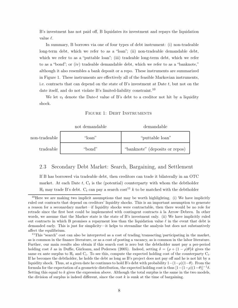
In summary, B borrows via one of four types of debt instrument: (i) non-tradeable

long-term debt, which we refer to as a “loan”; (ii) non-tradeable demandable debt,

which we refer to as a “puttable loan”; (iii) tradeable long-term debt, which we refer

to as a “bond”; or (iv) tradeable demandable debt, which we refer to as a “banknote,”

although it also resembles a bank deposit or a repo. These instruments are summarized

in Figure 1. These instruments are effectively all of the feasible Markovian instruments,

i.e. contracts that can depend on the state of B’s investment at Date t, but not on the

date itself, and do not violate B’s limited-liability constraint.10

We let vt denote the Date-t value of B’s debt to a creditor not hit by a liquidity

shock.

Figure 1: Debt Instruments

not demandable demandable

non-tradeable “loan” “puttable loan”

tradeable “bond” “banknote” (deposits or repos)

2.3 Secondary Debt Market: Search, Bargaining, and Settlement

If B has borrowed via tradeable debt, then creditors can trade it bilaterally in an OTC

market. At each Date t, Ct is the (potential) counterparty with whom the debtholder

Ht may trade B’s debt. Ct can pay a search cost11 k to be matched with the debtholder

10Here we are making two implicit assumptions that may be worth highlighting. (i) We have implicitlyruled out contracts that depend on creditors’ liquidity shocks. This is an important assumption to generatea reason for a seconardary market—if liquidity shocks were contractable, then there would be no role forretrade since the first best could be implemented with contingent contracts à la Arrow–Debreu. In otherwords, we assume that the Markov state is the state of B’s investment only. (ii) We have implicitly ruledout contracts in which B promises a repayment less than the liquidation value ℓ in the event that debt isdemanded early. This is just for simplicity—it helps to streamline the analysis but does not substantivelyaffect the equilibrium.

11This “search” cost can also be interpreted as a cost of trading/transacting/participating in the market,as is common in the finance literature, or as a cost of posting a vacancy, as is common in the labor literature.Further, our main results also obtain if this search cost is zero but the debtholder must pay a per-periodholding cost δ as in Duffie, Gârleanu, and Pedersen (2005). Indeed, setting δ =

(

ρ + (1 − ρ)θ)

k gives thesame ex ante surplus to Ht and Ct. To see this, compute the expected holding cost of the counterparty Ct.If he becomes the debtholder, he holds the debt as long as B’s project does not pay off and he is not hit by aliquidity shock. Thus, at a given date he continues to hold B’s debt with probability 1−(1−ρ)(1−θ). From theformula for the expectation of a geometric distribution, the expected holding cost is thus [1−(1−ρ)(1−θ)]−1δ.Setting this equal to k gives the expression above. Although the total surplus is the same in the two models,the division of surplus is indeed different, since the cost k is sunk at the time of bargaining.

8

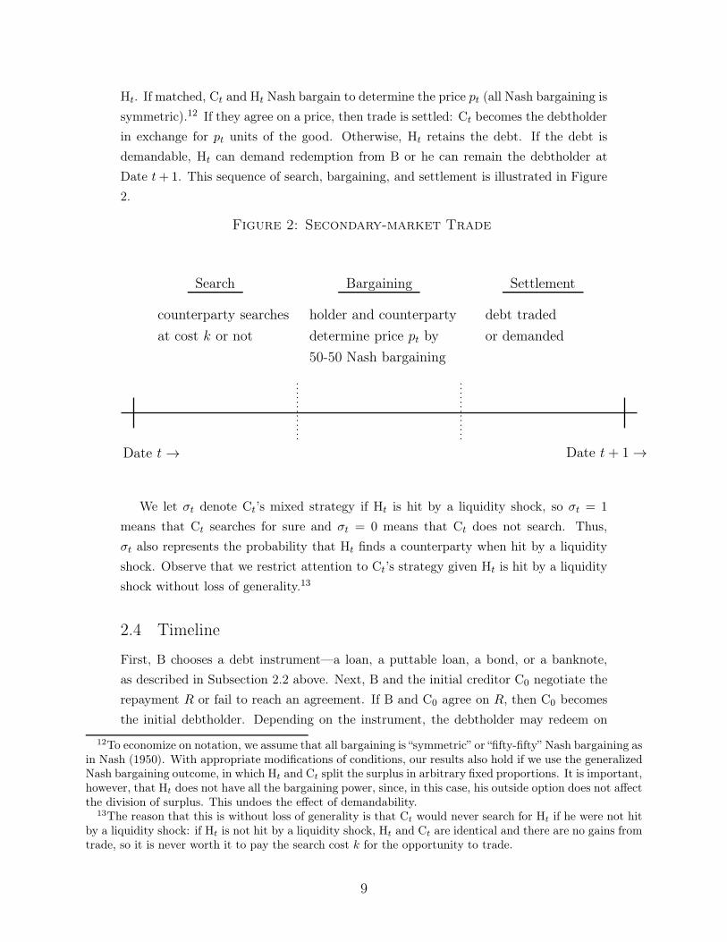
Ht. If matched, Ct and Ht Nash bargain to determine the price pt (all Nash bargaining is

symmetric).12 If they agree on a price, then trade is settled: Ct becomes the debtholder

in exchange for pt units of the good. Otherwise, Ht retains the debt. If the debt is

demandable, Ht can demand redemption from B or he can remain the debtholder at

Date t+ 1. This sequence of search, bargaining, and settlement is illustrated in Figure

2.

Figure 2: Secondary-market Trade

Date t → Date t+ 1 →

Search

counterparty searches

at cost k or not

Bargaining

holder and counterparty

determine price pt by

50-50 Nash bargaining

Settlement

debt traded

or demanded

We let σt denote Ct’s mixed strategy if Ht is hit by a liquidity shock, so σt = 1

means that Ct searches for sure and σt = 0 means that Ct does not search. Thus,

σt also represents the probability that Ht finds a counterparty when hit by a liquidity

shock. Observe that we restrict attention to Ct’s strategy given Ht is hit by a liquidity

shock without loss of generality.13

2.4 Timeline

First, B chooses a debt instrument—a loan, a puttable loan, a bond, or a banknote,

as described in Subsection 2.2 above. Next, B and the initial creditor C0 negotiate the

repayment R or fail to reach an agreement. If B and C0 agree on R, then C0 becomes

the initial debtholder. Depending on the instrument, the debtholder may redeem on

12To economize on notation, we assume that all bargaining is “symmetric” or “fifty-fifty” Nash bargaining asin Nash (1950). With appropriate modifications of conditions, our results also hold if we use the generalizedNash bargaining outcome, in which Ht and Ct split the surplus in arbitrary fixed proportions. It is important,however, that Ht does not have all the bargaining power, since, in this case, his outside option does not affectthe division of surplus. This undoes the effect of demandability.

13The reason that this is without loss of generality is that Ct would never search for Ht if he were not hitby a liquidity shock: if Ht is not hit by a liquidity shock, Ht and Ct are identical and there are no gains fromtrade, so it is never worth it to pay the search cost k for the opportunity to trade.

9

demand or may trade in the secondary market, as described in Subsection 2.3 above.

Formally, the extensive form is as follows.

Date 0 B chooses a debt instrument

B is matched with C0; B and C0 Nash bargain to determine the repayment

R

If B and C0 agree on R, then B invests c. C0 is the initial debtholder, H1 = C0

Date t > 0 If B’s investment pays off

B repays R to Ht and B consumes y −R

If B’s investment does not pay off: Ct and Ht search, bargain, and settle as

described in Subsection 2.3

If there is trade, Ct becomes the new debtholder, Ht+1 = Ct

If there is no trade, Ht either holds the debt, Ht+1 = Ht, or redeems on

demand, in which case B repays ℓ to Ht and B consumes zero

2.5 Equilibrium

The solution concept is subgame perfect equilibrium. An equilibrium constitutes (i) the

instrument and associated repayment R, (ii) the price of debt in the secondary market

pt at each date, and (iii) the search strategy σt of the potential counterparty Ct14 such

that B’s choice of instrument and Ct’s choice to search are sequentially rational, R and

pt are determined by Nash bargaining, and each player’s beliefs are consistent with

other players’ strategies and the outcomes of Nash bargaining.

We focus on pure, stationary equilibria, i.e. σt ≡ σ ∈ {0, 1} and pt ≡ p.

2.6 Assumption: Horizon Mismatch

We assume that parameters are such that there is a relatively severe horizon mis-

match between B’s investment and creditors’ liquidity needs, as in Diamond and Dybvig

(1983). In our infinite-horizon environment, this implies that the expected investment

horizon 1/ρ must be sufficiently large relative to the expected liquidity horizon 1/θ.

Specifically, we assume that the following condition holds:

1

ρ>

1

θ

2(y − c)

c (1 − ρ). (⋆)

14Formally, we could also include the debtholder’s choice whether to redeem on demand. We omit this,however, and just assume that the debtholder redeems on demand whenever he is hit by a liquidity shockand does not trade the debt. This assumption is just for simplicity; it does not affect the equilibrium.

10

This assumption implies that B intermediates between short-horizon creditors and a

long-horizon investment. This implies B resembles a bank, since, almost by definition,

banks transform maturity to meet the needs of short-term depositors and long-term

borrowers.

This assumption helps to present our most interesting/novel results in a simple way.

We do not need it to characterize the equilibrium. Indeed, we relax it in Subsection

3.8.

3 Results

In this section, we present our main results.

3.1 Borrowing Constraint

We begin the analysis with a necessary condition for B to be able to borrow enough to

fund its investment.

Lemma 1. For a given instrument, B can borrow and invest if and only if the Date-0

value of its debt exceeds the cost of investment, i.e. if and only if

v0 ≥ c ($)

for some repayment R ≤ y.

We make use of this borrowing constraint repeatedly below when we consider each type

of debt instrument in turn and ask whether B can borrow enough to undertake its

investment.

3.2 Loan

First, we consider a loan, i.e. non-tradeable long-term debt. At Date t, the value vt of

the loan can be written recursively:

vt = ρR+ (1− ρ)(1 − θ)vt+1. (1)

The terms are determined as follows. With probability ρ, B’s investment pays off and B

repays R. With probability (1−ρ)θ, B’s investment does not payoff and the debtholder

Ht is hit by a liquidity shock. Since the loan is neither tradeable nor demandable, Ht

gets zero. With probability (1 − ρ)(1 − θ), B’s investment does not pay off and Ht is

not hit by a liquidity shock. Ht retains B’s debt at Date t + 1, which has value vt+1

11

at Date t since there is no discounting.15 By stationarity (vt = vt+1 ≡ v), equation (1)

gives

v =ρR

ρ+ (1− ρ)θ. (2)

Given the horizon mismatch assumption (⋆), the expression above is always less than

the cost of investment c. Thus, if B borrows via a loan, B cannot satisfy its borrowing

constraint ($) and therefore cannot invest.

Lemma 2. If B borrows via a loan, it cannot fund its investment.

B cannot borrow from C0 via a loan even though its project has positive NPV. This

is because, given the horizon mismatch, C0 is likely to be hit by a liquidity shock and

need to consume before the project pays off, in which case C0 gets zero, since the loan

is neither tradeable nor demandable.

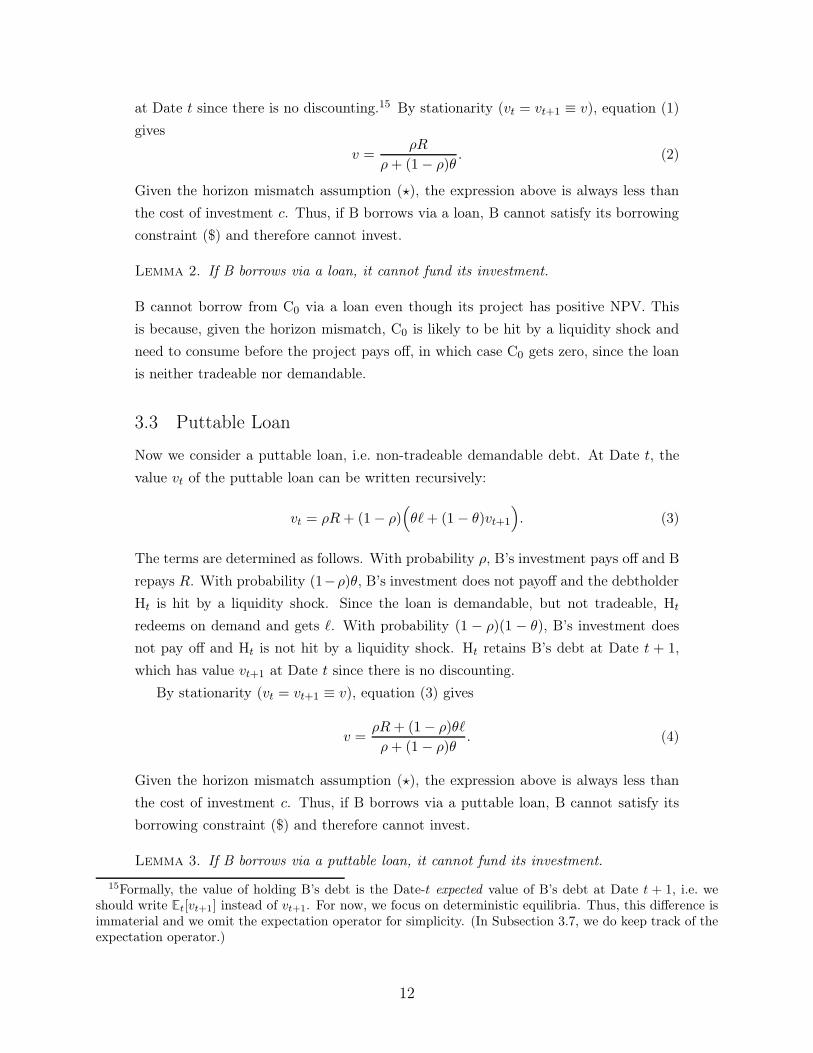
3.3 Puttable Loan

Now we consider a puttable loan, i.e. non-tradeable demandable debt. At Date t, the

value vt of the puttable loan can be written recursively:

vt = ρR+ (1− ρ)(

θℓ+ (1− θ)vt+1

)

. (3)



Ht is hit by a liquidity shock. Since the loan is demandable, but not tradeable, Ht

redeems on demand and gets ℓ. With probability (1 − ρ)(1 − θ), B’s investment does

not pay off and Ht is not hit by a liquidity shock. Ht retains B’s debt at Date t + 1,

which has value vt+1 at Date t since there is no discounting.

By stationarity (vt = vt+1 ≡ v), equation (3) gives

v =ρR+ (1− ρ)θℓ

ρ+ (1− ρ)θ. (4)


the cost of investment c. Thus, if B borrows via a puttable loan, B cannot satisfy its

borrowing constraint ($) and therefore cannot invest.

Lemma 3. If B borrows via a puttable loan, it cannot fund its investment.

15Formally, the value of holding B’s debt is the Date-t expected value of B’s debt at Date t + 1, i.e. weshould write Et[vt+1] instead of vt+1. For now, we focus on deterministic equilibria. Thus, this difference isimmaterial and we omit the expectation operator for simplicity. (In Subsection 3.7, we do keep track of theexpectation operator.)

12

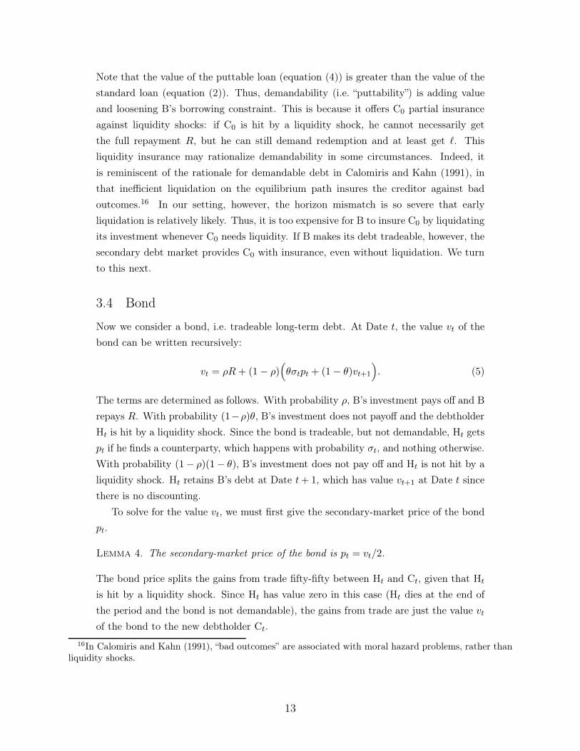
Note that the value of the puttable loan (equation (4)) is greater than the value of the

standard loan (equation (2)). Thus, demandability (i.e. “puttability”) is adding value

and loosening B’s borrowing constraint. This is because it offers C0 partial insurance

against liquidity shocks: if C0 is hit by a liquidity shock, he cannot necessarily get

the full repayment R, but he can still demand redemption and at least get ℓ. This

liquidity insurance may rationalize demandability in some circumstances. Indeed, it

is reminiscent of the rationale for demandable debt in Calomiris and Kahn (1991), in

that inefficient liquidation on the equilibrium path insures the creditor against bad

outcomes.16 In our setting, however, the horizon mismatch is so severe that early

liquidation is relatively likely. Thus, it is too expensive for B to insure C0 by liquidating

its investment whenever C0 needs liquidity. If B makes its debt tradeable, however, the

secondary debt market provides C0 with insurance, even without liquidation. We turn

to this next.

3.4 Bond

Now we consider a bond, i.e. tradeable long-term debt. At Date t, the value vt of the

bond can be written recursively:

vt = ρR+ (1− ρ)(

θσtpt + (1− θ)vt+1

)

. (5)



Ht is hit by a liquidity shock. Since the bond is tradeable, but not demandable, Ht gets

pt if he finds a counterparty, which happens with probability σt, and nothing otherwise.

With probability (1− ρ)(1− θ), B’s investment does not pay off and Ht is not hit by a

liquidity shock. Ht retains B’s debt at Date t+ 1, which has value vt+1 at Date t since

there is no discounting.

To solve for the value vt, we must first give the secondary-market price of the bond

pt.

Lemma 4. The secondary-market price of the bond is pt = vt/2.

The bond price splits the gains from trade fifty-fifty between Ht and Ct, given that Ht

is hit by a liquidity shock. Since Ht has value zero in this case (Ht dies at the end of

the period and the bond is not demandable), the gains from trade are just the value vt

of the bond to the new debtholder Ct.

16In Calomiris and Kahn (1991), “bad outcomes” are associated with moral hazard problems, rather thanliquidity shocks.

13

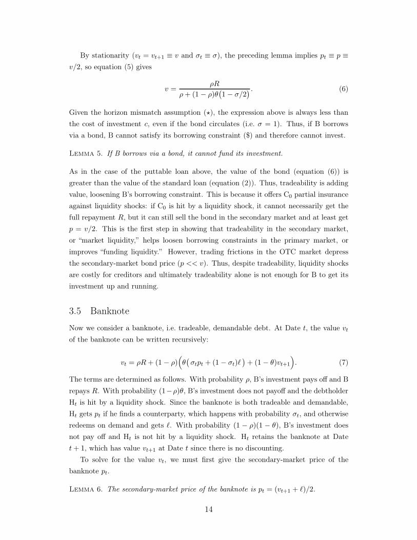
By stationarity (vt = vt+1 ≡ v and σt ≡ σ), the preceding lemma implies pt ≡ p ≡

v/2, so equation (5) gives

v =ρR

ρ+ (1− ρ)θ(

1− σ/2) . (6)


the cost of investment c, even if the bond circulates (i.e. σ = 1). Thus, if B borrows

via a bond, B cannot satisfy its borrowing constraint ($) and therefore cannot invest.

Lemma 5. If B borrows via a bond, it cannot fund its investment.

As in the case of the puttable loan above, the value of the bond (equation (6)) is

greater than the value of the standard loan (equation (2)). Thus, tradeability is adding

value, loosening B’s borrowing constraint. This is because it offers C0 partial insurance

against liquidity shocks: if C0 is hit by a liquidity shock, it cannot necessarily get the

full repayment R, but it can still sell the bond in the secondary market and at least get

p = v/2. This is the first step in showing that tradeability in the secondary market,

or “market liquidity,” helps loosen borrowing constraints in the primary market, or

improves “funding liquidity.” However, trading frictions in the OTC market depress

the secondary-market bond price (p << v). Thus, despite tradeability, liquidity shocks

are costly for creditors and ultimately tradeability alone is not enough for B to get its

investment up and running.

3.5 Banknote

Now we consider a banknote, i.e. tradeable, demandable debt. At Date t, the value vt

of the banknote can be written recursively:

vt = ρR+ (1− ρ)(

θ(

σtpt + (1− σt)ℓ)

+ (1− θ)vt+1

)

. (7)



Ht is hit by a liquidity shock. Since the banknote is both tradeable and demandable,

Ht gets pt if he finds a counterparty, which happens with probability σt, and otherwise

redeems on demand and gets ℓ. With probability (1 − ρ)(1 − θ), B’s investment does

not pay off and Ht is not hit by a liquidity shock. Ht retains the banknote at Date

t+ 1, which has value vt+1 at Date t since there is no discounting.

To solve for the value vt, we must first give the secondary-market price of the

banknote pt.

Lemma 6. The secondary-market price of the banknote is pt = (vt+1 + ℓ)/2.

14

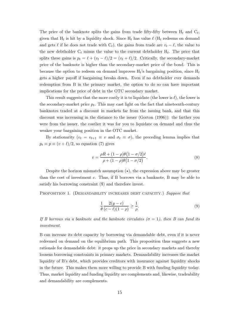
The price of the banknote splits the gains from trade fifty-fifty between Ht and Ct,

given that Ht is hit by a liquidity shock. Since Ht has value ℓ (Ht redeems on demand

and gets ℓ if he does not trade with Ct), the gains from trade are vt − ℓ, the value to

the new debtholder Ct minus the value to the current debtholder Ht. The price that

splits these gains is pt = ℓ+ (vt − ℓ)/2 = (vt + ℓ)/2. Critically, the secondary-market

price of the banknote is higher than the secondary-market price of the bond. This is

because the option to redeem on demand improves Ht’s bargaining position, since Ht

gets a higher payoff if bargaining breaks down. Even if no debtholder ever demands

redemption from B in the primary market, the option to do so can have important

implications for the price of debt in the OTC secondary market.

This result suggests that the more costly it is to liquidate (the lower is ℓ), the lower is

the secondary-market price pt. This may cast light on the fact that nineteenth-century

banknotes traded at a discount in markets far from the issuing bank, and that this

discount was increasing in the distance to the issuer (Gorton (1996)): the farther you

were from the issuer, the costlier it was for you to liquidate on demand and thus the

weaker your bargaining position in the OTC market.

By stationarity (vt = vt+1 ≡ v and σt ≡ σ), the preceding lemma implies that

pt ≡ p ≡ (v + ℓ)/2, so equation (7) gives

v =ρR+ (1− ρ)θ

(

1− σ/2)

ℓ

ρ+ (1− ρ)θ(

1− σ/2) . (8)

Despite the horizon mismatch assumption (⋆), the expression above may be greater

than the cost of investment c. Thus, if B borrows via a banknote, B may be able to

satisfy his borrowing constraint ($) and therefore invest.

Proposition 1. (Demandability increases debt capacity.) Suppose that

1

θ

2(y − c)

(c− ℓ)(1− ρ)≥

1

ρ. (9)

If B borrows via a banknote and the banknote circulates (σ = 1), then B can fund its

investment.

B can increase its debt capacity by borrowing via demandable debt, even if it is never

redeemed on demand on the equilibrium path. This proposition thus suggests a new

rationale for demandable debt: it props up the price in secondary markets and thereby

loosens borrowing constraints in primary markets. Demandability increases the market

liquidity of B’s debt, which provides creditors with insurance against liquidity shocks

in the future. This makes them more willing to provide B with funding liquidity today.

Thus, market liquidity and funding liquidity are complements and, likewise, tradeability

and demandability are complements.

15

3.6 Money Runs

Having established that B can borrow only with tradeable, demandable debt (ban-

knotes), we now turn to secondary-market liquidity and the possibility that a debtholder

demands early redemption. To do this, we assume that B has issued a banknote with

promised repayment R and look at the equilibria of the subgames for t > 0. (We

determine R in equilibrium in Proposition 3).

First, observe that B’s banknote indeed circulates as long as σt = 1 is a best response

to the belief that Ct′ plays σt′ = 1 for all t′ > t. This is the case as long as Ct is willing

to pay the search cost k to gain the surplus v − p given σ = 1, or

k ≤ v − p∣

∣

∣

σ=1

=ρ(R − ℓ)

2ρ+ (1− ρ)θ, (10)

having substituted in from Lemma 6 and equation (8).

But there may also be another equilibrium in which B’s banknote does not circulate.

B’s banknote does not circulate as long as σt = 0 is a best response to the belief that

Ct′ plays σt′ = 0 for all t′ > t. This is the case as long as Ct is not willing to pay the

search cost k to gain the surplus v − p given σ = 0, or

k ≥ v − p∣

∣

∣

σ=0=

1

2

ρ(R− ℓ)

ρ+ (1− ρ)θ, (11)

again having substituted in from Lemma 6 and equation (8).

Proposition 2. (Money runs.) Suppose that B borrows via a banknote with promised

repayment R and the search cost k is such that

1

2

ρ(R− ℓ)

ρ+ (1− ρ)θ≤ k ≤

ρ(R − ℓ)

2ρ+ (1− ρ)θ. (12)

The t > 0 subgame has both an equilibrium in which B’s debt debt circulates (σ = 1)

and there is no early liquidation and an equilibrium in which B’s debt does not circulate

(σ = 0) and there is early liquidation.

Thus demandable debt has a dark side: if a counterparty Ct doubts future liquidity,

i.e. he doubts that he will find a counterparty in the future, then Ct will not search. As

a result, the debtholder Ht indeed will not find a counterparty. There is a self-fulfilling

dry-up of secondary-market liquidity. With demandable debt, this has severe real ef-

fects: unable to trade, Ht redeems its debt on demand, leading to costly liquidation of

B’s investment. In other words, a change in just the beliefs about future liquidity leads

to the failure of B’s debt as a medium of exchange in the secondary market—the failure

of B’s debt as money. As a result, there is sudden withdrawal of liquidity from B, i.e.

a bank run, or a money run.

16

Corollary 1. Suppose k satisfies condition (12). If Ct’s beliefs change from σt′ = 1

to σt′ = 0 for t′ > t, the debtholder Ht “runs” on B, i.e. Ht unexpectedly demands

redemption of his debt, forcing B to liquidate its investment.

Demandability cuts both ways in the secondary market. It increases B’s debt capacity

by creating market liquidity, propping up the price of B’s debt. But it also exposes B

to money runs, since B must provide liquidity on demand if market liquidity dries up.

Thus, financial fragility may be a necessary evil, resulting from the need to overcome

funding constraints given a horizon mismatch between the investment and the creditors’

liquidity needs.

3.7 Equilibrium Runs

We now turn to characterizing an equilibrium in which B borrows via a banknote

and money runs arise on the equilibrium path. To do this, we expand the model

slightly to introduce a “sunspot” coordination variable at each date, st ∈ {0, 1}. We

will interpret st = 1 as “normal times” and st = 0 as a “confidence crisis,” since the

sunspot does not affect economic fundamentals, but serves only as a way for agents to

coordinate their beliefs. We assume that s0 = 1, that P [st+1 = 0 | st = 1] =: λ, and

that P [st+1 = 0 | st = 0] = 1, where we think about λ as a small number. In words:

the economy starts in normal times and a permanent confidence crisis occurs randomly

with small probability λ.

We now look for a Markov equilibrium, i.e. an equilibrium in which the sunspot

(rather than the whole history) is a sufficient statistic for Ct’s action:

σt =

σ1 if st = 1,

σ0 if st = 0.(13)

Note that the baseline case of a stationary equilibrium is the special case of λ = 0.

We can now write the banknote’s value v0 when st = 0 and v1 when st = 1 (cf. the

analogous equation for the stationary case in equation (7)):

v0 = ρR+ (1− ρ)

(

θ(

σ0p0 +(

1− σ0)

ℓ)

+ (1− θ)v0

)

, (14)

v1 = ρR+ (1− ρ)

(

θ(

σ1p1 +(

1− σ1)

ℓ)

+ (1− θ)(

λv0 + (1 − λ)v1)

)

. (15)

The next proposition characterizes an equilibrium in which the “confidence crisis” in-

duces a money run.

Proposition 3. (Equilibrium with sunspot runs.) Suppose that the condition in

17

equation (9) is satisfied. As long as λ is sufficiently small, there exists k such that B

can fund its investment only with tradeable, demandable debt (a banknote), even though

it admits a money run when st = 0. Specifically, Ct plays σt = st, and the value of the

banknote when st = 0 is

v0 =ρR+ (1− ρ)θℓ

ρ+ (1− ρ)θ(16)

the value of the banknote when st = 1 is

v1 =ρR+ (1− ρ)

(

θℓ/2 + (1− θ/2)λv0

)

ρ+ (1− ρ)(

θ/2 + (1− θ/2)λ) , (17)

and the promised repayment is

R = y −

(

ρ+ (1− ρ)θ)(

ρ+ (1− ρ)λ)

ρ(

ρ+ (1− ρ)(

θ + (1− θ)λ)

)

(

v1 − c)

. (18)

We have written the system recursively, expressing v1 as a function of v0 and R as

a function of v1, for simplicity. We give a closed-form expression for R in terms of

primitives in Appendix 3.

3.8 Circulating Bonds and Liquidity Dry-ups without Runs

So far, we have maintained the horizon mismatch assumption (⋆), which implied that

only the banknote was feasible. In this section, we relax this assumption, so that bonds

are feasible too. We find that bonds have two advantages over banknotes: (i) they are

more liquid in the secondary market, which can help with financing, and (ii) they are

not subject to runs, which can prevent inefficient liquidation.

Proposition 4. (Bond finance.) Suppose that

1

θ

y − c

(c− ℓ)(1− ρ)≤

1

ρ≤

1

θ

2(y − c)

c(1 − ρ), (19)

andρ(y − ℓ)

2ρ+ (1− ρ)θ≤ k ≤

ρy

2ρ+ (1− ρ)θ. (20)

B can fund its investment only with tradeable, long-term debt (a bond).

Intuitively, this result says that if there is a horizon mismatch which is not too severe

(condition (19)), then B can borrow via a bond, but cannot borrow via a non-circulating

instrument, such as a puttable loan. And, further, if the search cost k is large enough

(condition (20)), then B cannot borrow via a banknote either. The reason is that

demandability increases secondary-market prices, which can discourage search: whereas

18

a counterparty may be willing to pay k to search for a bond, since he anticipates buying

at a discount, he may be reluctant to pay k to search for a banknote, since he anticipates

paying a high price. Thus, the banknote may not circulate—and a non-circulating

banknote is effectively just a puttable loan.

Even though a counterparty is relatively willing to pay k to search for a bond,

liquidity dry-ups can still occur in the secondary market for the bond.

Corollary 2. Suppose that B borrows via a bond with promised repayment R and that

1

2

ρR

ρ+ (1− ρ)θ≤ k ≤

ρR

2ρ+ (1− ρ)θ. (21)

The t > 0 subgame has both an equilibrium in which B’s debt debt circulates (σ = 1)

and an equilibrium in which B’s debt does not circulate (σ = 0). However, there is not

early liquidation in either equilibrium; B’s investment always pays off y.

Like trade in banknotes, trade in bonds is self-fulfilling. A self-fulfilling liquidity dry-

up can arise whenever a counterparty searches if and only if he believes that other

counterparties will search in the future (cf. equations (10) and (11) in Subsection 3.6).

However, since the bond is not demandable, liquidity dry-ups in the secondary market

do not lead to runs or inefficient liquidation of B’s investment.

The analysis above captures the two advantages that bonds have over banknotes:

(i) dry-ups in bond liquidity are “less likely” than dry-ups in banknote liquidity, since

counterparties search for bonds for larger k, and (ii) they are less costly, since they do

not lead to B’s liquidation. Thus, we expect to see demandable debt mainly when the

horizon mismatch is so severe that borrowing via bonds is impossible. We think this

casts light on why bank debt is more likely to be demandable than corporate debt: the

horizon mismatch assumption (⋆) is more likely to hold for banks than for other firms.

4 Conclusion

One important function of banks is to create money, i.e. to issue debt that circulates

in OTC markets. By focusing on this function of banks, we found a new type of bank

runs—“money runs”—and a new rationale for demandable debt, both of which are the

result of how bank debt circulates—or fails to circulate—in secondary markets. Money

runs occur because secondary-market liquidity is fragile and self-fulfilling. Banks issue

demandable debt because its secondary-market price is high. In contrast to the liter-

ature, our results suggest that financial fragility may be a necessary evil and, further,

that regulating markets may help bank stability more than regulating banks themselves.

19

A Proofs

A.1 Proof of Lemma 1

The result follows immediately from C0’s participation constraint: B and C0 find an

agreement point if and only if bargaining gives both more than their disagreement

utilities. Since C0 receives v0 from bargaining, this must exceed its cost c.


By Lemma 1, B can invest only if v0 = v ≥ c or, by equation (2),

ρR

ρ+ (1− ρ)θ≥ c. (22)

This says that1

θ

R− c

c (1 − ρ)≥

1

ρ(23)

which violates the assumption (⋆) since R ≤ y.



ρR+ (1− ρ)θℓ

ρ+ (1− ρ)θ≥ c. (24)

Since ℓ < c/2, a necessary condition for this is that

ρR+ (1− ρ)θc/2

ρ+ (1− ρ)θ≥ c. (25)

This says that1

θ

2 (R − c)

c (1 − ρ)≥

1

ρ(26)



When Ct and Ht are matched Ht has been hit by a liquidity shock. Thus, Ct’s value

of the bond is vt and Ht’s value of the bond is zero (since Ht consumes only at Date t

and the bond is not demandable). The total surplus is thus vt, which Ct and Ht split

fifty-fifty in accordance with the Nash bargaining solution. Thus the price is pt = vt/2.

20



ρR

ρ+ (1− ρ)θ(

1− σ/2) ≥ c. (27)

This is increasing in σ, so a necessary condition is that the above holds for σ = 1, or

ρR

ρ+ (1− ρ)θ/2≥ c. (28)

This says that1

θ

2 (R − c)

c (1 − ρ)≥

1

ρ(29)



When Ct and Ht are matched Ht has been hit by a liquidity shock. Thus, Ct’s value of

the banknote is vt and Ht’s value of the banknote is ℓ (since Ht consumes only at Date

t, it redeems on demand if it does not trade). The gains from trade are thus vt − ℓ,

which Ct and Ht split fifty-fifty in accordance with the Nash bargaining solution, i.e.

pt is such that

Ht gets1

2

(

vt − ℓ)

+ ℓ = pt, (30)

Ct gets1

2

(

vt − ℓ)

= vt − pt, (31)

or pt = (vt + ℓ)/2.

A.7 Proof of Proposition 1

By Lemma 1, B can invest if v0 = v ≥ c or, by equation (8) with σ = 1,

2ρR+ (1− ρ)θℓ

2ρ+ (1− ρ)θ≥ c. (32)

This says that1

θ

2 (R − c)

(c− ℓ) (1− ρ)≥

1

ρ. (33)

This is feasible for some R ≤ y, i.e. as long as

1

θ

2 (y − c)

(c− ℓ) (1− ρ)≥

1

ρ, (34)

21

which is the condition in the proposition (note this is mutually compatible with the

horizon mismatch assumption (⋆)).


The argument is in the text.

A.9 Proof of Corollary 1

The result follows immediately from Proposition 2.


We first solve for the values v0 and v1 given the strategies σ0 = 0 and σ1 = 1. We then

show that these strategies are indeed best responses (for some k). Finally, we compute

the repayment R in accordance with the Nash bargaining solution.

Values. From equation (14) with σ0 = 0, we have immediately that

v0 =ρR+ (1− ρ)θℓ

ρ+ (1− ρ)θ(35)

(this is just the value of the puttable loan in equation (4)). From Lemma 6 (the logic

of which is not affected by the presence of sunspots), we have the price

p1 =λv0 + (1− λ)v1 + ℓ

2. (36)

Thus, equation (15) with σ1 = 1 reads

v1 = ρR+ (1− ρ)

(

θλv0 + (1− λ)v1 + ℓ

2+ (1− θ)

(

λv0 + (1− λ)v1)

)

, (37)

so

v1 =ρR+ (1− ρ)

(

θℓ/2 + (1− θ/2)λv0

)

ρ+ (1− ρ)(

θ/2 + (1− θ/2)λ) (38)

Best responses. σ1 = 1 and σ0 = 0 are best response if

v0 − p0 ≤ k ≤ v1 − p1 (39)

or

v0 −v0 + ℓ

2≤ k ≤ v1 −

λv0 + (1− λ)v1 + ℓ

2. (40)

This is satisfied for some k as long as v1 ≥ v0, which is the case as long as R ≥ ℓ, which

must be the case.

22

Repayment. The repayment R is determined by Nash bargaining between B and

C0. Now denote B’s value in state s by us. Since the state is s = 1 at Date 0, B and

C0 agree on a repayment R such that B’s value is u1 and C0’s value is v1. The gains

from trade are thus u1 + v1 − c. R is thus such that

B gets1

2

(

u1 + v1 − c)

= u1, (41)

C0 gets1

2

(

u1 + v1 − c)

+ c = v1, (42)

so u1 = v1 − c.

From the expressions above we can compute R in terms of primitives. First we

compute B’s value u0 in state 0. In this case, the banknote does not circulate and the

banknote is effectively like the puttable loan in Subsection 3.3. Whenever the creditor

is hit by a liquidity shock, he redeems on demand and B liquidates and gets zero. B’s

value is thus

u0 = ρ(y −R) + (1− ρ)(1− θ)u0 (43)

or

u0 =ρ(y −R)

ρ+ (1− ρ)θ. (44)

Now, B’s value in state 1 is given by

u1 = ρ(y −R) + (1− ρ)(

(1− λ)u1 + λ(1− θ)u0)

(45)

or, substituting in for u0 from equation (44) above,

u1 =ρ(y −R)

ρ+ (1− ρ)λ

(

1 +(1− ρ)λ(1− θ)

ρ+ (1− ρ)θ

)

. (46)

Substituting for this into the bargaining outcome u1 = v1 − c gives the expression for

the repayment R in terms of v1 as stated in the proposition.

Now we can also substitute for v1 from equation (38) and v0 from equation (35)

above to get

R =Ay +Bc− Cℓ

D(47)

23

where the constants A, B, C, and D are defined as follows:

A =(

2(

ρ+ (1− ρ)λ+ (1− ρ)(1− λ)θ)(

(

ρ+ (1− ρ)θ)(

ρ+ (1− ρ)λ)

− (1− ρ)θλ)

,

B =(

2(

ρ+ (1− ρ)λ+ (1− ρ)(1− λ)θ)

(

ρ+ (1− ρ)θ)(

ρ+ (1− ρ)λ)

,

C =(

ρ+ (1− ρ)λ)

(1− ρ)(

ρ+ (1− ρ)(

2λ+ (1− λ)θ)

)

,

D = ρ(

θ(5 + 4λ)(1 − ρ)(

ρ+ (1− ρ)λ)

+ θ2(1− λ)2(1− ρ)2 + 4(

ρ+ (1− ρ)λ)2)

.


We first show that for k satisfying condition (20), the bond can circulate but the

banknote cannot. We then show that if the bond circulates, B can fund its investment

with a bond. However, if the banknote does not circulate, B cannot fund its investment

with a banknote. This also implies that B cannot fund its investment with a puttable

loan or a loan: a puttable loan is identical to a non-circulating banknote, which is

infeasible, and a puttable loan always has higher debt capacity than a loan (cf. equations

(2) and (4)).

Bond can circulate. The bond circulates whenever Ct’s value v less the price p

exceeds his cost of searching k, or, given the value in equation (6) and the price in

Lemma 4,1

2

ρR

ρ+ (1− ρ)θ(1− σ/2)≥ k. (48)

For R = y and σ = 1 this reads

ρy

2ρ+ (1− ρ)θ≥ k, (49)

which is satisfied by assumption (condition (20)). Thus, the bond can circulate as long

as R is sufficiently large.

Banknote cannot circulate. The banknote circulates whenever Ct’s value v less

the price p exceeds his cost of searching k, or, given the value in equation (8) and the

price in Lemma 6,1

2

ρ(R− ℓ)

ρ+ (1− ρ)θ(1− σ/2)≥ k. (50)

The left-hand side is maximized when R = y and σ = 1, for which the inequality reads

ρ(y − ℓ)

2ρ+ (1− ρ)θ≥ k, (51)

which is never satisfied by assumption (condition (20)). Thus, the banknote cannot

circulate.

Bond financing feasible. Given the bond circulates (σ = 1), the borrowing

24

constraint ($) is satisfied whenever

ρR

ρ+ (1− ρ)θ/2≥ c, (52)

given the value of the bond from equation (6). This can be re-written as

1

ρ≤

1

θ

2(R − c)

c(1 − ρ). (53)

This is satisfied by assumption (condition (19)) as long as R is sufficiently large.

Banknote financing infeasible. Given the banknote does not circulate (σ = 0),

the borrowing constraint ($) is satisfied whenever

ρR+ (1− ρ)θℓ

ρ+ (1− ρ)θ≥ c, (54)

given the value of the banknote from equation (8). This can be re-written as

1

ρ≤

1

θ

R− c

(c− ℓ)(1 − ρ). (55)

The right-hand side is maximized when R = y, for which the inequality reads

1

ρ≤

1

θ

y − c

(c− ℓ)(1 − ρ). (56)

This is never satisfied by assumption (condition (19)).

A.12 Proof of Corollary 2

The argument here is analogous to the argument for the banknote in Subsection 3.6:

there are multiple equilibria whenever (i) a counterparty’s searching is a best response

other counterparties’ searching and (ii) a counterparty’s not searching is a best response

to other counterparties’ not searching, or

v − p∣

∣

∣

σ=0≤ k ≤ v − p

∣

∣

∣

σ=1. (57)

Substituting in for the value of the bond v from equation (6) and the price of the bond

p from Lemma 4, this reads

1

2

ρR

ρ+ (1− ρ)θ≤ k ≤

ρR

2ρ+ (1− ρ)θ, (58)

as stated in the corollary.

25

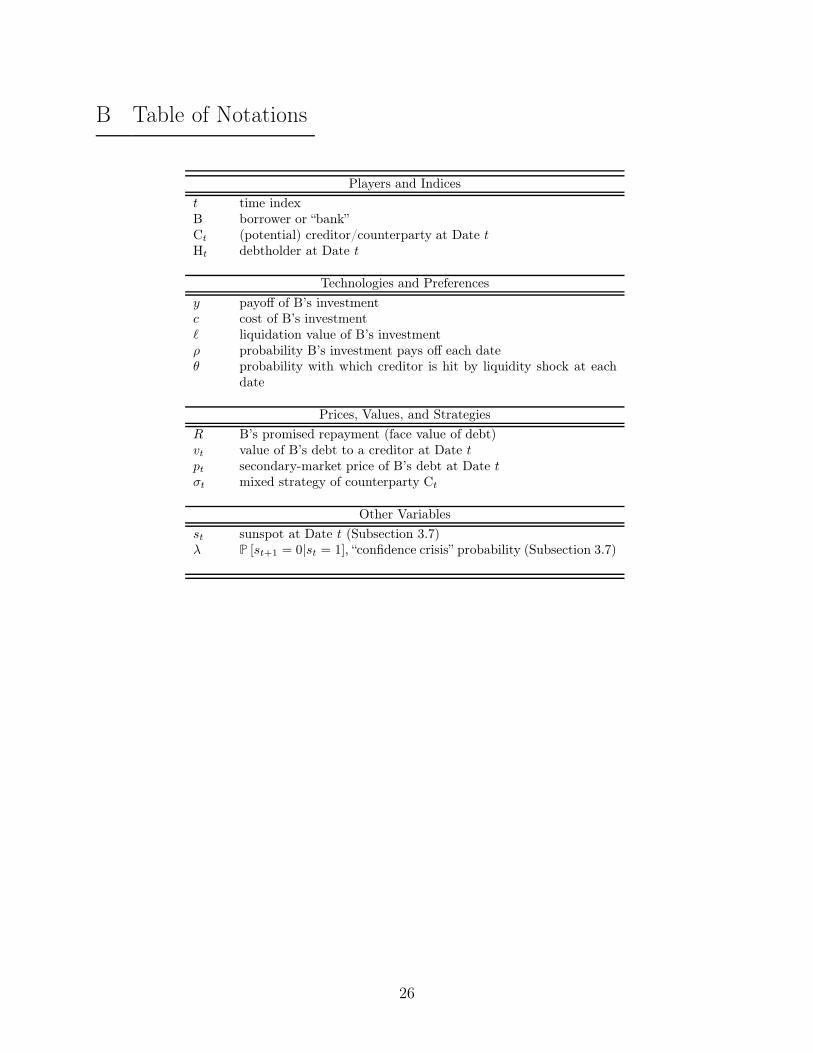
B Table of Notations

Players and Indices

t time indexB borrower or “bank”Ct (potential) creditor/counterparty at Date tHt debtholder at Date t

Technologies and Preferences

y payoff of B’s investmentc cost of B’s investmentℓ liquidation value of B’s investmentρ probability B’s investment pays off each dateθ probability with which creditor is hit by liquidity shock at each

date

Prices, Values, and Strategies

R B’s promised repayment (face value of debt)vt value of B’s debt to a creditor at Date tpt secondary-market price of B’s debt at Date tσt mixed strategy of counterparty Ct

Other Variables

st sunspot at Date t (Subsection 3.7)λ P [st+1 = 0|st = 1], “confidence crisis” probability (Subsection 3.7)

26

References

Allen, Franklin, and Douglas Gale, 2004, Financial intermediaries and markets, Econo-

metrica 72, 1023–1061.

Andolfatto, David, Ed Nosal, and Bruno Sultanum, 2017, Preventing bank runs, The-

oretical Economics forthcoming.

Antinolfi, Gaetano, and Suraj Prasad, 2008, Commitment, banks and markets, Journal

of Monetary Economics 55, 265 – 277.

Bruche, Max, and Anatoli Segura, 2016, Debt maturity and the liquidity of secondary

debt markets, Temi di discussione (Economic working papers) 1049 Bank of Italy,

Economic Research and International Relations Area.

Burdett, Kenneth, Alberto Trejos, and Randall Wright, 2001, Cigarette money, Journal

of Economic Theory 99, 117–142.

Calomiris, Charles W, and Charles M Kahn, 1991, The role of demandable debt in

structuring optimal banking arrangements, American Economic Review 81, 497–513.

Champ, Bruce, Bruce D. Smith, and Stephen D. Williamson, 1996, Currency elasticity

and banking panics: theory and evidence, Canadian Journal of Economics 29, 828–

864.

Dang, Tri Vi, Gary Gorton, and Bengt Hölmstrom, 2015a, Ignorance, debt and financial

crises, Working paper.

, 2015b, The information sensitivity of a security, Working paper.

, and Guillermo Ordoñez, 2017, Banks as secret keepers, American Economic

Review forthcoming.

Diamond, Douglas W, 1997, Liquidity, banks, and markets, Journal of Political Econ-

omy 105, 928–56.

Diamond, Douglas W., and Philip H. Dybvig, 1983, Bank runs, deposit insurance, and

liquidity, Journal of Political Economy 91, 410–419.

Diamond, Douglas W., and Raghuram G. Rajan, 2001a, Banks and liquidity, The

American Economic Review 91, 422–425.

, 2001b, Liquidity risk, liquidty creation, and financial fragility: A theory of

banking, Journal of Political Economy 109, 287–327.

27

Donaldson, Jason Roderick, Giorgia Piacentino, and Anjan Thakor, 2016, Warehouse

banking, Working paper Washington University in St Louis.

Duffie, Darrell, Nicolae Gârleanu, and Lasse Heje Pedersen, 2005, Over-the-counter

markets, Econometrica 73, 1815–1847.

Gorton, Gary, 1996, Reputation formation in early bank note markets, Journal of

Political Economy 104, 346–97.

, and Andrew Metrick, 2012, Securitized banking and the run on repo, Journal

of Financial Economics 104, 425–451.

Gorton, Gary, and Guillermo Ordoñez, 2014, Collateral crises, American Economic

Review 104, 343–78.

Gorton, Gary, and George Pennacchi, 1990, Financial intermediaries and liquidity

creation, Journal of Finance 45, 49–71.

Gorton, Gary B., 2012a, Misunderstanding Financial Crises: Why We Don’t See Them

Coming (Oxford University Press).

, 2012b, Some reflections on the recent financial crisis, NBER Working Papers

18397 National Bureau of Economic Research, Inc.

, and Andrew Metrick, 2009, Haircuts, NBER Working Papers 15273 National

Bureau of Economic Research, Inc.

Green, Edward J., and Ping Lin, 2003, Implementing efficient allocations in a model of

financial intermediation, Journal of Economic Theory 109, 1–23.

Gu, Chao, Fabrizio Mattesini, Cyril Monnet, and Randall Wright, 2013, Banking: a

new monetarist approach, Review of Economic Studies 80, 636–662.

He, Zhiguo, and Konstantin Milbradt, 2014, Endogenous liquidity and defaultable

bonds, Econometrica 82, 1443–1508.

He, Zhiguo, and Wei Xiong, 2012, Dynamic debt runs, Review of Financial Studies 25,

1799–1843.

Jacklin, Charles, 1987, Demand deposits, trading restrictions, and risk sharing, in Ed-

ward Prescott, and Neil Wallace, ed.: Contractual Arrangements for Intertemporal

Trade . chap. II, pp. 26–47 (University of Minnesota Press: Minneapolis).

, 1989, Demand equity and deposit insurance, Working paper Stanford Univer-

sity.

28

Kiyotaki, Nobuhiro, and John Moore, 2001, Evil is the root of all money, Clarendon

Lectures, Oxford.

Kiyotaki, Nobuhiro, and Randall Wright, 1989, On money as a medium of exchange,

Journal of Political Economy 97, 927–954.

, 1993, A search-theoretic approach to monetary economics, American Economic

Review 83, 63–77.

Krishnamurthy, Arvind, Stefan Nagel, and Dmitry Orlov, 2014, Sizing up repo, The

Journal of Finance 69, 2381–2417.

Kuong, John, 2015, Self-fulfilling fire sales: Fragility of collateralised short-term debt

markets, Working paper.

Lee, Jeongmin, 2015, Collateral circulation and repo spreads, Working paper Washing-

ton University in St Louis.

Leland, Hayne, and Klaus Bjerre Toft, 1996, Optimal capital structure, endogenous

bankruptcy, and the term structure of credit spreads, Journal of Finance 51, 987–

1019.

Martin, Antoine, David Skeie, and Ernst-Ludwig von Thadden, 2014a, The fragility

of short-term secured funding markets, Journal of Economic Theory 149, 15 – 42

Financial Economics.

, 2014b, Repo runs, Review of Financial Studies.

Nash, John F., 1950, The bargaining problem, Econometrica 18, 155–162.

Peck, James, and Karl Shell, 2003, Equilibrium bank runs, Journal of Political Economy

111, 103–123.

Sanches, Daniel, 2016, On the inherent instability of private money, Review of Economic

Dynamics 20, 198–214.

Sanches, Daniel R., 2015, Banking panics and protracted recessions, Working Papers

15-39 Federal Reserve Bank of Philadelphia.

Singh, Manmohan, 2010, The velocity of pledged collateral, Working paper IMF.

, and James Aitken, 2010, The (sizable) role of rehypothecation in the shadow

banking system, Working paper IMF.

29

Trejos, Alberto, and Randall Wright, 1995, Search, bargaining, money, and prices,

Journal of Political Economy 103, 118–41.

Vanasco, Victoria, 2016, The Downside of asset screening for market liquidity, Journal

of Finance.

von Thadden, Ernst-Ludwig, 1999, Liquidity creation through banks and markets: Mul-

tiple insurance and limited market access, European Economic Review 43, 991 – 1006.

30

jason roderick donaldson giorgia piacentino march … runs∗ jason roderick donaldson† giorgia...

Documents