jaquelino nascimento da rosa - connecting repositories · the future for batch polymerization...
TRANSCRIPT
September, 2011
MODELING AND SIMULATION OF A LAB-SCALEPOLYMERIZATION REACTOR
Unive
rsida
de d
e Co
imbra
MODE
LING
AND
SIMUL
ATION
OF A
LAB
-SCAL
E PO
LYME
RIZAT
ION
REAC
TOR
Jaque
lino
Nasci
mento
da Ro
sa
Jaquelino Nascimento da Rosa

Departamento de Engenharia Química
Faculdade de Ciências e Tecnologia
Universidade de Coimbra
Modeling and Simulation of a Lab-Scale
Polymerization Reactor
Dissertação apresentada à Faculdade de Ciências e Tecnologia da Universidade deCoimbra, com vista à obtenção do grau de Mestre em Engenharia Química.
Jaquelino Nascimento da Rosa
Orientadores:
Jorge Fernando CoelhoLino de Oliveira Santos
Coimbra, Setembro de 2011


“The simplest explanationis most likely the correct one.”William of Ockham
To my beloved teacher,Maria Margarida Lopes Figueiredo


Abstract
The main goal of this work is to study the thermal dynamics of a lab-scale vesselthat can be used for polymerization experiments. It involves a study of the ther-mal dynamics of a 250 mL jacketed lab-scale glass reactor intended to be used inthe future for batch polymerization reaction experiments. A mathematical model isdeveloped and is used to simulate the thermal dynamics of the system. The math-ematical model available in the literature for methyl methacrylate (MMA) solutionfree-radical polymerization is also considered in this simulation study. The numer-ical implementation of the models has been made in the MATLAB programminglanguage. The simulation results of the lab-scale reactor show the heating and cool-ing performance, and a feedback control scheme using a split-range control strategyis tested as well to simulate the temperature setpoint tracking of the MMA polymer-ization mixture in the lab-scale reactor.


Resumo
Neste trabalho é efectuado um estudo térmico de um reactor laboratorial em vidro,dotado de uma camisa de arrefecimento/aquecimento e com uma capacidade de 250mL. Prentende-se no futuro utilizar este reactor para realizar ensaios experimentaisde polimerização. É formulado um modelo matemático do reactor e é simuladonumericamente o seu comportamento dinâmico. O estudo desenvolvido inclui tam-bém o modelo matemático para a polimerização de metacrilato de metilo (MMA) emsolução em modeo descontínuo, disponibilizado na literatura cientÃfica. A imple-mentação numérica dos modelos matemáticos é efectuada com recurso à linguagemde programação MATLAB. Os resultados de simulação demonstram o desempenhotérmico do reactor, nomeadamente a sua capacidade de resposta quando é aquecidoou arrefecido. É também apresentado um estudo do reactor sob controlo por reali-mentação da temperatura da mistura do sistema de polimerização de MMA, em queé adoptada uma estratégia de controlo do tipo split-range.


Acknowledgements
First and foremost, I would like to express my sincere gratitude to my supervi-sors, Dr Jorge Coelho and Dr Lino Santos, who have supported me throughout mydissertation with their guidance, patience, motivation, enthusiasm, knowledge andfriendship whilst allowing me the room to work in my own way.
I am truly indebted and thankful to Dr Nuno Oliveira for having provided veryuseful numerical data from Silva (2005).
I would like to gratefully and sincerely thank my high school teachers, Elisân-gela Semedo, Teodorino Carvalho, João Pedro Semedo, Augusto Borges, and ÂngelaVarela, for their continuous support during my dissertation and my graduate studies.
I would like to thank my mother, Hermínia Veiga, and my family for their support,encouragement and unwavering love.
I offer my regards and blessings to the whole DEQ community and all of thosewho supported me in any respect during the completion of this work.

Nomenclature
A heat transfer area m2
Cp,j jacket fluid heat capacity J kg−1K−1
Cp,r reaction medium heat capacity J kg−1K−1
d impeller diameter mDH hydraulic diameter mDi reactor internal diameter mDn dead polymer concentration with n repeating units mol m−3
Do reactor internal diameter mfi initiator efficiency factorFj jacket volumetric flow rate m3min−1
f(m,n) weight fraction of polymer in chain length interval [m, n]gt gel effect parameterhi internal heat transfer coefficient W m−2K−1
ho external heat transfer coefficient W m−2K−1
I initiator concentration mol m−3
k thermal conductivity W m−1K−1
Kc PID controller gainkd initiator decomposition rate constant min−1
kfm chain transfer to monomer rate constant m3 mol−1min−1
kfs chain transfer to solvent rate constant m3 mol−1min−1
ki primary radical formation rate constant m3 mol−1min−1
kp propagation rate constant m3 mol−1min−1
ktd disproportionation termination rate constant m3 mol−1min−1
M monomer concentration mol m−3
mc PID controller command signalMt total reaction mass kgMn number average molecular weight kg mol−1
Mw weight average molecular weight kg mol−1
N impeller rotational speed rad min−1
Nu Nusselt numberP total concentration of live polymer radicals mol m−3
Pn live polymer radical concentration with n repeating units mol m−3
Pr Prandtl numberR primary radical concentration mol m−3
Re Reynolds numberRH hydraulic radius mS solvent concentration mol m−3
Tj jacket fluid temperature ◦C

viii
Tj,0 jacket fluid initial temperature ◦CTr reaction medium temperature ◦CU overall heat transfer coefficient calculation W m−2K−1
Ueff effective overall heat transfer coefficient calculation W m−2K−1
V reaction mixture volume Lvf free volumevfcr critical free volumeVj jacket volume m3
wi initiator mass fractionwm monomer mass fractionwm,0 monomer initial mass fractionws solvent mass fractionwp polymer mass fractionX monomer conversiony measured value for the controlled variableysp controlled variable setpoint
Greek Lettersα probability of propagation∆H heat of reaction J mol−1
∆t sampling time minεk controller error signalλk kth moment of dead polymer molecular weight distributionµ reaction medium viscosity Pa sµw reaction medium viscosity at wall temperature Pa sρm monomer density kg m−3
ρp polymer density kg m−3
ρs solvent density kg m−3
τD derivative time minτI integral time minφm monomer volume fractionφp polymer volume fractionφs solvent volume fraction
AcronymsCLD chain length distributionMMA methyl methacrylateMWD molecular weight distributionODE ordinary differential equationPID proportional/integral/derivativePMMA Poly(methyl methacrylate)PTFE polytetrafluoroethyleneSISO single input, single outputWCLD weight chain length distribution

Contents
Abstract i
Resumo iii
Acknowledgements v
Nomenclature vii
List of Tables xi
List of Figures xiii
1. Introduction 11.1. Thesis outline . . . . . . . . . . . . . . . . . . . . . . . . . . . . . . . . . 2
2. Batch Solution Free-radical Polymerization of Methyl Methacrylate (MMA) 32.1. MMA free-radical polymerization kinetics . . . . . . . . . . . . . . . . 32.2. Dynamic model formulation . . . . . . . . . . . . . . . . . . . . . . . . 5
2.2.1. Molecular weight averages and MWD from molecular weightmoments . . . . . . . . . . . . . . . . . . . . . . . . . . . . . . . . 5
2.2.2. Mass and energy balances . . . . . . . . . . . . . . . . . . . . . . 72.2.3. Numerical implementation . . . . . . . . . . . . . . . . . . . . . 92.2.4. Temperature control with a PID controller . . . . . . . . . . . . 11
3. Lab-scale Polymerization Reactor 173.1. Lab-scale reactor open-loop thermal study . . . . . . . . . . . . . . . . 17
3.1.1. Perfectly mixed jacket . . . . . . . . . . . . . . . . . . . . . . . . 183.1.2. Plug flow cooling jacket . . . . . . . . . . . . . . . . . . . . . . . 223.1.3. Lumped jacket model . . . . . . . . . . . . . . . . . . . . . . . . 24
3.2. MMA polymerization in the lab-scale reactor . . . . . . . . . . . . . . . 253.2.1. Split-range control . . . . . . . . . . . . . . . . . . . . . . . . . . 263.2.2. Simulation results . . . . . . . . . . . . . . . . . . . . . . . . . . 27
4. Conclusions 354.1. Future work . . . . . . . . . . . . . . . . . . . . . . . . . . . . . . . . . . 35
Bibliography 37
ix
x Contents
A. Overall heat transfer coefficient 43A.1. Internal heat transfer coefficient . . . . . . . . . . . . . . . . . . . . . . 43A.2. External heat transfer coefficient calculation . . . . . . . . . . . . . . . 44A.3. Overall heat transfer coefficient . . . . . . . . . . . . . . . . . . . . . . . 44
B. Heat transfer area 45
C. Physical properties of fluids 47C.1. Water . . . . . . . . . . . . . . . . . . . . . . . . . . . . . . . . . . . . . . 47
C.1.1. Heat capacity . . . . . . . . . . . . . . . . . . . . . . . . . . . . . 47C.1.2. Density . . . . . . . . . . . . . . . . . . . . . . . . . . . . . . . . . 47C.1.3. Viscosity . . . . . . . . . . . . . . . . . . . . . . . . . . . . . . . . 48C.1.4. Thermal conductivity . . . . . . . . . . . . . . . . . . . . . . . . 48
C.2. Ethyl acetate . . . . . . . . . . . . . . . . . . . . . . . . . . . . . . . . . . 48C.2.1. Heat capacity . . . . . . . . . . . . . . . . . . . . . . . . . . . . . 48C.2.2. Density . . . . . . . . . . . . . . . . . . . . . . . . . . . . . . . . . 48
C.3. Methyl methacrylate (MMA) . . . . . . . . . . . . . . . . . . . . . . . . 48C.3.1. Heat capacity . . . . . . . . . . . . . . . . . . . . . . . . . . . . . 48C.3.2. Density . . . . . . . . . . . . . . . . . . . . . . . . . . . . . . . . . 48
C.4. Poly(methyl methacrylate) (PMMA) . . . . . . . . . . . . . . . . . . . . 49C.4.1. Heat capacity . . . . . . . . . . . . . . . . . . . . . . . . . . . . . 49C.4.2. Density . . . . . . . . . . . . . . . . . . . . . . . . . . . . . . . . . 49
D. Kinetic Parameters 51
E. MATLAB simulation programs 53E.1. Thermal study . . . . . . . . . . . . . . . . . . . . . . . . . . . . . . . . . 53
E.1.1. model function . . . . . . . . . . . . . . . . . . . . . . . . . . . . 53E.1.2. Main program . . . . . . . . . . . . . . . . . . . . . . . . . . . . . 55
E.2. MMA polymerization reaction study . . . . . . . . . . . . . . . . . . . . 60E.2.1. Model function . . . . . . . . . . . . . . . . . . . . . . . . . . . . 60E.2.2. Main program . . . . . . . . . . . . . . . . . . . . . . . . . . . . . 64E.2.3. PID controller function . . . . . . . . . . . . . . . . . . . . . . . 77E.2.4. Function for the calculation of monomer, polymer and solvent
densities . . . . . . . . . . . . . . . . . . . . . . . . . . . . . . . . 78

List of Tables
2.1. Kinetic scheme for the free-radical polymerization of MMA (Crowleyand Choi, 1998) . . . . . . . . . . . . . . . . . . . . . . . . . . . . . . . . 5
2.2. Parameters for the MMA polymerization reaction (Crowley and Choi,1998). . . . . . . . . . . . . . . . . . . . . . . . . . . . . . . . . . . . . . . 9
2.3. Initial conditions for the polymerization reaction (Crowley and Choi,1997b). . . . . . . . . . . . . . . . . . . . . . . . . . . . . . . . . . . . . . 9
2.4. Molecular weight averages for 50% conversion. . . . . . . . . . . . . . 102.5. PID controller parameters: controlled variable - Tr; manipulated vari-
able - Tj,0. . . . . . . . . . . . . . . . . . . . . . . . . . . . . . . . . . . . . 12
3.1. Range for the manipulated variables, Fhot and Fcold. . . . . . . . . . . . 273.2. Parameters for the MMA polymerization reaction. . . . . . . . . . . . . 273.3. PID controller parameters: controlled variable - Tr; manipulated vari-
ables - Fhot and Fcold. The application of the tuning method describedin Section 2.2.4 is illustrated in Figure 3.13. . . . . . . . . . . . . . . . . 29
A.1. The typical values for the empirical correlation constants (Debab et al.,2011). . . . . . . . . . . . . . . . . . . . . . . . . . . . . . . . . . . . . . . 43
B.1. Lab-scale reactor dimensions. . . . . . . . . . . . . . . . . . . . . . . . . 45
C.1. Molecular weight of monomer (methyl methacrylate), solvent (Ethylacetate) and initiator (2,2’-azobis(2-methylbutanenitrile)) (Ellis et al.(1988)). . . . . . . . . . . . . . . . . . . . . . . . . . . . . . . . . . . . . . 47
D.1. Kinetic parameters for the MMA solution polymerization, with [T] =K (Crowley and Choi (1997b)). . . . . . . . . . . . . . . . . . . . . . . . 52
xi

List of Figures
2.1. MMA free radical polymerization reaction scheme (A. - initiation, B. -propagation, C. - chain transfer to monomer and solvent, D. - termi-nation by disproportionation). Adapted from Kranjk et al. (2001). . . . 4
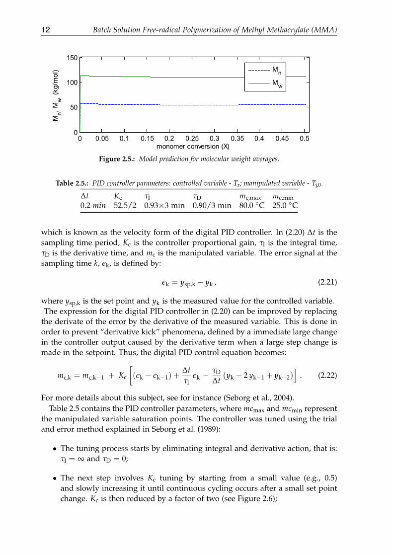
2.2. Monomer conversion model prediction. . . . . . . . . . . . . . . . . . . 102.3. Model MWD prediction. . . . . . . . . . . . . . . . . . . . . . . . . . . . 112.4. Model prediction for monomer conversion. . . . . . . . . . . . . . . . . 112.5. Model prediction for molecular weight averages. . . . . . . . . . . . . . 122.6. PID controller tuning. Kc - Proportional gain, τI - Integral time, and
τD - Derivative time. . . . . . . . . . . . . . . . . . . . . . . . . . . . . . 132.7. PID control of reactor temperature in the MMA batch solution poly-
merization reactor. . . . . . . . . . . . . . . . . . . . . . . . . . . . . . . 142.8. Manipulated variable (Tj,0) dynamics under the PID control. . . . . . . 142.9. Ratio between the heat transfered and the reaction heat. . . . . . . . . 15
3.1. Lab-scale reactor. . . . . . . . . . . . . . . . . . . . . . . . . . . . . . . . 183.2. Water-water system. Tr and Tj profiles for the cooling simulation. . . 193.3. Water-water system. Physical properties of the fluids inside the reac-
tor and jacket for the cooling simulation. . . . . . . . . . . . . . . . . . 193.4. Water-water system. Tr and Tj profiles for the heating simulation. . . 203.5. Water-water system. Physical properties of the fluids inside the reac-
tor and jacket for the heating simulation. . . . . . . . . . . . . . . . . . 203.6. Water-organic system. Tr and Tj profiles for the heating simulation. . 213.7. Water-organic system. Physical properties of the fluids inside the re-
actor and jacket for the heating simulation. . . . . . . . . . . . . . . . . 213.8. Water-water system. Plug flow cooling jacket with the cooling fluid at
80◦C. . . . . . . . . . . . . . . . . . . . . . . . . . . . . . . . . . . . . . . 223.9. Water-water system. Lumped jacket with the cooling fluid at 80◦C. . 233.10. Water-water system. Lumped temperatures (Tj,i, i = 1, 4). . . . . . . . 243.11. Stabilization time dependence on cooling fluid flow rate and temper-
ature. . . . . . . . . . . . . . . . . . . . . . . . . . . . . . . . . . . . . . . 253.12. Variable overall heat transfer coefficient (U) significance. . . . . . . . . 263.13. PID controller tuning. Kc - Proportional gain, τI - Integral time, and
τD - Derivative time. . . . . . . . . . . . . . . . . . . . . . . . . . . . . . 283.14. Monomer conversion and reactor temperature evolution. . . . . . . . . 293.15. Monomer, solvent, initiator and live radical molar concentrations. . . 293.16. Mass fraction of the solvent and the initiator. . . . . . . . . . . . . . . . 30
xiii

xiv List of Figures
3.17. Molecular weight moments. . . . . . . . . . . . . . . . . . . . . . . . . . 303.18. Number and weight average molecular weights. . . . . . . . . . . . . . 303.19. Molecular weight distribution at the final instant of the reaction. . . . 313.20. Evolution of the molecular weight distribution during the reaction time. 313.21. Jacket temperature (Tj), hot and cold fluid flow rate in the jacket (Thot =
85◦C and Tcold = 25◦C) and controller command signal (mc) in the in-terval t = [10, 60]min. . . . . . . . . . . . . . . . . . . . . . . . . . . . . . 32
3.22. Jacket temperature (Tj), hot and cold fluid flow rate in the jacket (Thot =
85◦C and Tcold = 25◦C) and controller command signal (mc) profiles. 323.23. Jacket temperature (Tj), hot and cold fluid flow rate in the jacket (Thot =
85◦C and Tcold = 25◦C) and controller command signal (mc) profileswith derivative kick. . . . . . . . . . . . . . . . . . . . . . . . . . . . . . 33
B.1. Representation of the lab-scale polymerization reactor. . . . . . . . . . 45

1. Introduction
Polymerization reactions pose some specific challenges in contrast to ordinary reac-tion systems through the necessity of, not only monitoring the conversion, but alsothe polymer molecular weight distribution (MWD) has to be maintained in order toproduce polymers of acceptable quality. The strong nonlinearities of polymerizationreactors make it even more difficult to control a polymerization reactor (Adebekunand Schork, 1989).
The solution polymerization of methyl methacrylate (MMA) in a lab-scale batchreactor, proceeded by the free-radical mechanism is the system studied in this work,with ethyl acetate as the solvent and 2,2’-azobis(2-methylbutanenitrile) as the radicalinitiator. This system was chosen due to great versatility of poly(methyl methacry-late) (PMMA), providing it a wide range of applications, and also to the fact that alarge amount of information can be found in the literature.
The number average molecular weight (Mn) and weight average molecular weight(Mw) are convenient polymer characterization parameters as they represent compactand convenient information about a polymerization system. Mn is more sensitiveto molecules of low molecular weight, while Mw has the opposite behavior. Theratio between Mw and Mn is called polydispersity and it measures the breadth ofthe polymer MWD. Nevertheless, polymers with similar polydispersity value mayexhibit significantly different MWD and, consequently, different end-use properties.Therefore, to fully characterize a polymer MWD a new method is needed and themethod of finite molecular weight moments, presented in Crowley and Choi (1997a)can, conveniently, sort out this issue. This method approximates the infinite molecu-lar weight domain by a number of finite chain length intervals, each one containinga determined weight fraction of polymer. The number of intervals is established sothat a good resolution of MWD is achieved, and the maximum chain length is chosenso that the chain length domain encompasses at least 99.9% of polymer weight. Witha polymerization kinetic model, molecular weight averages and molecular weightdistribution can be determined by integrating the mass balance equations simulta-neously with the method of molecular weight moments.
A reliable control system is mandatory in polymerization reactors since changesin MWD may reveal irreversible, but also to prevent thermal runaway. More chal-lenges are added by the fact of the reaction taking place in a batch reactor, whichis characterized by having a nonlinear behavior and time-varying characteristics un-like continuous reactors, as pointed out by Silva and Oliveira (2002). There is a needto remove the reaction heat due to the exothermic nature of MMA polymerizationreaction (Adebekun and Schork, 1989), but heating is also required, especially at thebeginning of reaction, to raise the temperature to its desired value. In order to ac-
1

2 Introduction
complish both heating and cooling tasks, a split range control strategy is adopted,where the output of the controller is split to the hot and cold streams (Seborg et al.,2004). Split range controllers can have different arrangements, but for this work thecold stream is turned on when the controller signal is between 0 and 50% while thehot stream remains closed and when the controller signal is between 50 and 100%the hot stream is turned on while the cold stream is turned off (Section 3.2.1).
In batch polymerization reactors, the temperature is often maintained by manipu-lating the coolant temperature or its flow rate. Sometimes, to overcome the nonlinearnature of the process and the poor dynamics of heat removal, especially caused bygel effect, the control performance can be recovered by employing a cascade controlstrategy: a master controller which sets the reactor temperature setpoint for coolanttemperature, and a slave controller to control the coolant temperature by manipulat-ing the coolant flow rate into the jacket (Schork et al., 1993).
1.1. Thesis outline
Chapter 2 describes the batch solution free-radical polymerization of methyl methacry-late (MMA) system. The dynamic model is stated and its numerical implementationis developed. A comparison of the results obtained by simulation is made withexperimental data available in (Crowley and Choi, 1997b), and simulated profilesobtained in (Silva, 2005). In Chapter 3 the description of the lab-scale vessel reactoris introduced together with a study of the thermal dynamics of the heating and cool-ing processes. These studies required the development of the lab-scale reactor modeland of simulation programs written in MATLAB. Section 3.1 assesses the thermalbehavior of the vessel without any reaction through several heating and cooling sim-ulations. Here, several modeling approaches for the lab-scale vessel jacket are eval-uated. In Section 3.2 the mathematical model of the lab-scale reactor is formulatedto include the MMA polymerization reaction. Simulation results are presented withtemperature control performed by a PID controller. A split-range control strategythat manipulates a hot and cold water stream entering the reactor jacket is consid-ered in this study as well. Finally, the main conclusions and future work directionsare given in Chapter 4.

2. Batch Solution Free-radicalPolymerization of MethylMethacrylate (MMA)
Poly(methyl methacrylate) (PMMA) is a transparent thermoplastic used in a widerange of fields including medicine, art and aesthetics. It is also often used as analternative to glass due to its shatter-resistance property (Arora et al., 2010). Thischapter focus on the simulation of a solution free-radical polymerization of methylmethacrylate. The reaction takes place in a batch reactor operating mode which iswidely used in commercial production of polymer solutions of high-quality resins(Rantow and Soroush, 2005). The batch reactor model for this system is taken fromCrowley and Choi (1997a). The results obtained by simulation are compared withsimulation and experimental data from literature (Crowley and Choi, 1997b; Silva,2005) in order to validate the numerical implementation. This simulation study ad-dresses as well a single-input single-output (SISO) PID control system to controlthe reactor temperature to its desired value during the course of the polymerizationreaction.
The resulting polymer in a polymerization process is characterized not only byits average molecular weight but also by its molecular weight distribution (MWD).The control of the polymer chain length distribution (CLD) and of the correspond-ing MWD is of paramount importance because of end-use properties such as tensilestrength and impact strength that are strongly dependent on the MWD (Crowleyand Choi, 1997a). For instance, polymers with distinct MWD have different melt-ing points as well as different melted polymer flow properties (Ellis et al., 1988). Themolecular weight distribution and the average molecular weight, which are the num-ber average molecular weight (Mn) and the weight average molecular weight (Mw),can be calculated based on the polymerization kinetic model (e.g., see Table 2.1), andusing the method of molecular weight moments described in Section 2.2.1.
2.1. MMA free-radical polymerization kinetics
The kinetic scheme of the free-radical polymerization of MMA is presented in Ta-ble 2.1. It comprises the initiation step, where the initiator (I) decomposes to formreactive radicals (R), the addition of monomer molecules (M) to the reactive polymerchain formed from the reactive radicals, the chain transfer to monomer and sol-vent, and the termination step where deactivation of polymer radicals occur and
3
4 Batch Solution Free-radical Polymerization of Methyl Methacrylate (MMA)
CH3 CH2
C N
N C CH2
CH3CH3
C
CH3
C
N
N
N N CH3 CC
CH2
CH3
N
2+
CH3 C
C
CH2
CH3
N
+ CH2 C
CH3
C O
O CH3
CH3 C
C
CH2
CH3
N
CH2 CC O
OCH3
CH3
CH3 C
C
CH2
CH3
N
CH2 CC O
OCH3
CH3
+ CH2 C
CH3
C O
OCH3
n
CH3 C
C
CH2
CH3
N
CH2 C
CH3
COO
CH3
CH2 CC O
OCH3
CH3
CH3 C
C
CH2
CH3
N
CH2 C
CH3
COO
CH3
CH2 CC O
OCH3
CH3
CH3 C
C
CH2
CH3
N
CH2 C
CH3
COO
CH3
CH2 CC O
OCH3
CH3
+
CH3 C
C
CH2
CH3
N
CH2 C
CH3
COO
CH3
CH2 CC O
OCH3
CH3
HCH3 C
C
CH2
CH3
N
CH2 C
CH3
COO
CH3
CH CC O
OCH3
CH3
+
A.
C.
n
n m
n m
B.
CH3 C
C
CH2
CH3
N
CH2 C
CH3
COO
CH3
CH2 CC O
OCH3
CH3
n
+CH3
C
O
O
CH2
CH3
CH3 C
C
CH2
CH3
N
CH2 C
CH3
COO
CH3
CH2 C
C OO
CH3
CH3
CH2
CH3
n
+
CH3 C
C
CH2
CH3
N
CH2 C
CH3
COO
CH3
CH2 CC O
OCH3
CH3
n
+
n
+CH2 C
CH3
C O
OCH3
CH3
C
O
O
CH3 C
C
CH2
CH3
N
CH2 C
CH3
COO
CH3
CH2 C
C OO
CH3
CH3
CH3 CH2 C
CH3
C O
O
D.
∆
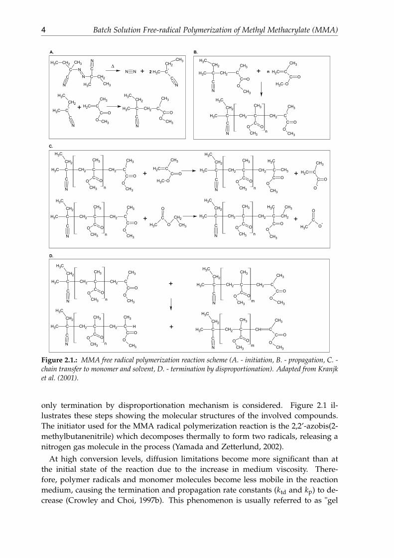
Figure 2.1.: MMA free radical polymerization reaction scheme (A. - initiation, B. - propagation, C. -chain transfer to monomer and solvent, D. - termination by disproportionation). Adapted from Kranjket al. (2001).
only termination by disproportionation mechanism is considered. Figure 2.1 il-lustrates these steps showing the molecular structures of the involved compounds.The initiator used for the MMA radical polymerization reaction is the 2,2’-azobis(2-methylbutanenitrile) which decomposes thermally to form two radicals, releasing anitrogen gas molecule in the process (Yamada and Zetterlund, 2002).
At high conversion levels, diffusion limitations become more significant than atthe initial state of the reaction due to the increase in medium viscosity. There-fore, polymer radicals and monomer molecules become less mobile in the reactionmedium, causing the termination and propagation rate constants (ktd and kp) to de-crease (Crowley and Choi, 1997b). This phenomenon is usually referred to as "gel

2.2 Dynamic model formulation 5
Table 2.1.: Kinetic scheme for the free-radical polymerization of MMA (Crowley and Choi, 1998). Iis the initiator, R is the primary radical, Pn is the live polymer radical with n repeating units, Dn isthe dead polymer with n repeating units, and S is the solvent.
Initiation: Ikd−→ 2R
R + Mki−→ P1
Propagation: Pn + Mkp−→ Pn+1
Chain transfer to monomer and solvent: Pn + Mkfm−→ Dn + P1
Pn + Skfs−→ Dn + P1
Termination (disproportionation only): Pn + Pmktd−→ Dn + Dm
effect" and a correlation is provided in the literature to account for this conditioninto the disproportionation termination rate constant (see Appendix D).
2.2. Dynamic model formulation
Modeling is a process used in science and engineering to describe systems, anda good mathematical model must adequately describe the experimental data on arange of conditions as large as possible and must be easily manipulated in order tobe useful in complex systems (Curteanu et al., 1998). A complete model for the MMApolymerization reaction system that can give information about MWD comprisesmass and energy balance equations, and molecular weight moment equations. Themodel for this system can be found in several works (e.g., Crowley and Choi 1997b).The mathematical description of the molecular weight distribution time-dependencyis given in Section 2.2.1. Then, the mass and energy balances are presented in Sec-tion 2.2.2.
2.2.1. Molecular weight averages and MWD from molecularweight moments
The molecular weight averages, namely the number average molecular weight (Mn)and weight average molecular weight (Mw) are insufficient to characterize a polymeras it is possible for two polymers with similar Mn and Mw to have distinct MWD and,consequently, substantially different physical and mechanical properties (Crowleyand Choi, 1997a). Thus, there is a need for a method to compute the polymer MWDand the method of the molecular weight moments is the one considered in this study.For dead polymers, the molecular weight moments are defined by:
λk =∞
∑n=2
nkDnV , (2.1)
6 Batch Solution Free-radical Polymerization of Methyl Methacrylate (MMA)
where λk represents the kth moment of a dead polymer, and V is the volume ofthe mixture. Since the concentration of live polymer (Pn) is negligible compared tothe concentration of dead polymer (Dn), then its moment is not considered for thecalculation of molecular weights (Crowley and Choi, 1997b). It follows that,
Mn = M0λ1
λ0and Mw = M0
λ2
λ1. (2.2)
To calculate the MWD, the following function is used to represent the weight fractionof polymer with molecular weight in the interval [m, n]:
f(m,n) =∑n
i=m iDiV∑∞
i=2 iDiV. (2.3)
The molecular weight distribution is time-dependent and the derivative of (2.3) withrespect to time is given by:
d f(m,n)
dt=
1λ1
n
∑i=m
id[DiV]
dt−
f(m,n)
λ1
dλ1
dt. (2.4)
From the kinetic scheme in Table 2.1, the kinetic rate equation for dead polymers ofchain length n can be derived:
d[DnV]
dt= V[ktdP + kfmM + kfsS]Pn . (2.5)
The following equation defines the probability of propagation α (Crowley and Choi,1997a),
α =kpM
kpM + kfmM + kfsS + ktdP. (2.6)
The summation term in (2.4) is determined by manipulating (2.5) and (2.6) such that
n
∑i=m
id[DiV]
dt= VkpM
1− α
α
n
∑i=m
iPi . (2.7)
Using the following relationship,
Pn = αPn−1 = (1− α)αn−1P , (2.8)
the term ∑ni=m iPi in (2.7) is given by:
n
∑i=m
iPi =
[m(1− α) + α
1− α
]αm−1P−
[(n + 1)(1− α) + α
1− α
]αnP . (2.9)

2.2 Dynamic model formulation 7
Finally, using the result in (2.9), equation (2.4) becomes
d f(m,n)
dt=
kpMVλ1
([m(1− α) + α
α
]αm−1−[
(n + 1)(1− α) + α
α
]αn)
P−f(m,n)
λ1
dλ1
dt.
(2.10)
Further details on these developments can be found for instance in Crowley and Choi(1997b). To determine the evolution of the MWD, the equation (2.10) is discretizedwith respect to the chain length distribution. The resulting number of differentialequations depends on the number of intervals considered for the weight chain lengthdistribution (WCLD). Crowley and Choi (1997b) used 15 intervals that increase as thechain length is increased (2.11), by defining:
m = 2 + a(i− 1)i , (2.11a)
n = 1 + ai(i + 1) , (2.11b)
with i = 1, ..., 15. The parameter a is selected such that that 99.9% of the resultingpolymer has a chain length between 2 to (1 + 15a(15 + 1)), that is,
f (2, 1 + 15a(15 + 1)) = 0.999 . (2.12)
2.2.2. Mass and energy balances
The mass and energy balances for this polymerization system can be found, forinstance, in the works of Silva (2005), Crowley and Choi (1997b, 1998), and Ellis et al.(1988). The partial mass balance to the monomer is expressed by:
dXdt
=(kp + kfm)wmP
wm,0, (2.13)
where X is the monomer conversion, wm is the monomer mass fraction, P is the totalconcentration of live polymer radicals, wm,0 is the initial monomer mass fraction,and kp and kfm are respectively the propagation rate constant and the chain transferto monomer rate constant. The partial mass balances to the initiator and solvent aregiven by:
dwi
dt= −kdwi , (2.14a)
dws
dt= −kfswsP , (2.14b)
where wi is the initiator mass fraction, and ws is the solvent mass fraction. Themolecular weight moment equations are also included to allow the calculation ofmolecular weight averages and MWD. The differential equations for the the zero,first, and second order moment of dead polymer MWD (λ0, λ1, and λ2) are defined

8 Batch Solution Free-radical Polymerization of Methyl Methacrylate (MMA)
by:
dλ0
dt= kpMV(1− α)P , (2.15a)
dλ1
dt= kpMV(2− α)P , (2.15b)
dλ2
dt=
kpMV(α2 − 3α + 4)P1− α
. (2.15c)
The energy balances to the reaction mixture and the jacket result in the followingequations:
dTr
dt=
(−∆H)kpwmMtP−UA(Tr − Tj)
ρrCp,rV, (2.16a)
dTj
dt=
FjρjCp,j(Tj,0 − Tj) + UA(Tr − Tj)
ρjCp,jVj, (2.16b)
where Tr and Tj are the reactor and jacket temperature, respectively.
Now, including (2.10) for MWD evaluation, the dynamic model of the batch so-lution free-radical polymerization of MMA is summarized into the following set ofequations:
dXdt
=(kp + kfm)wmP
wm,0, (2.17a)
dwi
dt= −kdwi , (2.17b)
dws
dt= −kfswsP , (2.17c)
dλ0
dt= kpMV(1− α)P , (2.17d)
dλ1
dt= kpMV(2− α)P , (2.17e)
dλ2
dt=
kpMV(α2 − 3α + 4)P1− α
, (2.17f)
dTr
dt=
(−∆H)kpwmMtP−UA(Tr − Tj)
ρrCp,rV, (2.17g)
dTj
dt=
FjρjCp,j(Tj,0 − Tj) + UA(Tr − Tj)
ρjCp,jVj, (2.17h)
d f(m,n)
dt=
kpMVλ1
([m(1− α) + α
α
]αm−1−[
(n + 1)(1− α) + α
α
]αn)
P−f(m,n)
λ1
dλ1
dt,
(2.17i)
2.2 Dynamic model formulation 9
Table 2.2.: Parameters for the MMA polymerization reaction (Crowley and Choi, 1998).
V Vj A Fj Ueff1.0 L 3.5 L 530.0 cm2 1.0 kgmin−1 817.0 calK−1min−1
Table 2.3.: Initial conditions for the polymerization reaction (Crowley and Choi, 1997b).
I0 φm,0 φs,00.046 molL−1 0.5 0.5
In equation (2.17), the total concentration of live polymers (P) is determined by
P =
(2 fikd I
ktd
)1/2
, (2.18)
where fi is the initiator efficiency factor which corresponds to the fraction of primaryradicals utilized in the chain growth (Kranjk et al., 2001).
Considering an ideal mixture and neglecting the initiator contribution, the totalreactor mixture volume, V, is given by:
V =
(wm
ρm+
wp
ρp+
ws
ρs
)Mt , (2.19)
where Mt is the total mass inside the reactor, wp is polymer mass fraction, and ρm,ρp, and ρs are the monomer, polymer, and solvent densities, respectively.
2.2.3. Numerical implementation
The numerical implementation of the model described in Section 2.2 was tested andthe obtained results were compared with experimental and simulated data avail-able in the literature. Crowley and Choi (1997b) provide experimental data for theconversion evolution for this polymerization system, as well as data for the kineticparameters, reactor characteristics, and initial conditions (see tables 2.2 and 2.3, andAppendix D). In these simulation studies the energy balance equations were not con-sidered because the results published by Crowley and Choi (1997b) were obtainedfor a scenario where the reactor temperature is chosen as a task level manipulatedvariable.
In tables 2.2 and 2.3, Ueff is the effective heat transfer coefficient (UA), I0 is theinitial concentration of the initiator, and φm,0 and φs,0 correspond to the monomerand solvent initial volume fraction, respectively.
With the information in these two tables, kinetic parameters in appendix D andphysical properties of the compounds present in the reacting system in AppendixC, the dynamic model (2.17) was solved using the MATLAB ODE solver ode15s,with a sampling period of 1.0 min. The resulting monomer conversion profile isshown in Figure 2.2. As it is presented in Crowley and Choi (1997b), the reactor

10 Batch Solution Free-radical Polymerization of Methyl Methacrylate (MMA)
0 50 100 1500
0.1
0.2
0.3
0.4m
onom
er c
onve
rsio
n (X
)
0 50 100 15050
60
time [min]
T r [ºC
]
simulationCrowley and Choi, 1997b
Figure 2.2.: Monomer conversion model prediction.
Table 2.4.: Molecular weight averages for 50% conversion.Mn (kg mol−1) Mw (kg mol−1)
model prediction 55.9 111.6Silva, 2005 55.1 109.9
mixture temperature was initially set at a temperature of 65 ◦C. Then, when themonomer conversion is of 27%, the reactor mixture is cooled down to 50 ◦C in orderto broaden the MWD (Crowley and Choi, 1997b). Figure 2.2 shows that the predictedmonomer conversion profile is similar to the one presented by Crowley and Choi(1997b), which is in good agreement with their experimental monomer conversionvalues. Remark that the reactor temperature change is simulated here by a stepchange. Although this approach is somewhat unrealistic, from the profiles providedin Crowley and Choi (1997b) it follows that the temperature dynamics appear to beconsiderably faster than the monomer concentration dynamics. In Section 2.2.4 aPID loop is considered to control the reactor mixture temperature.
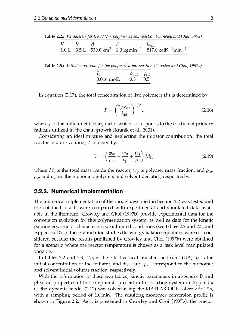
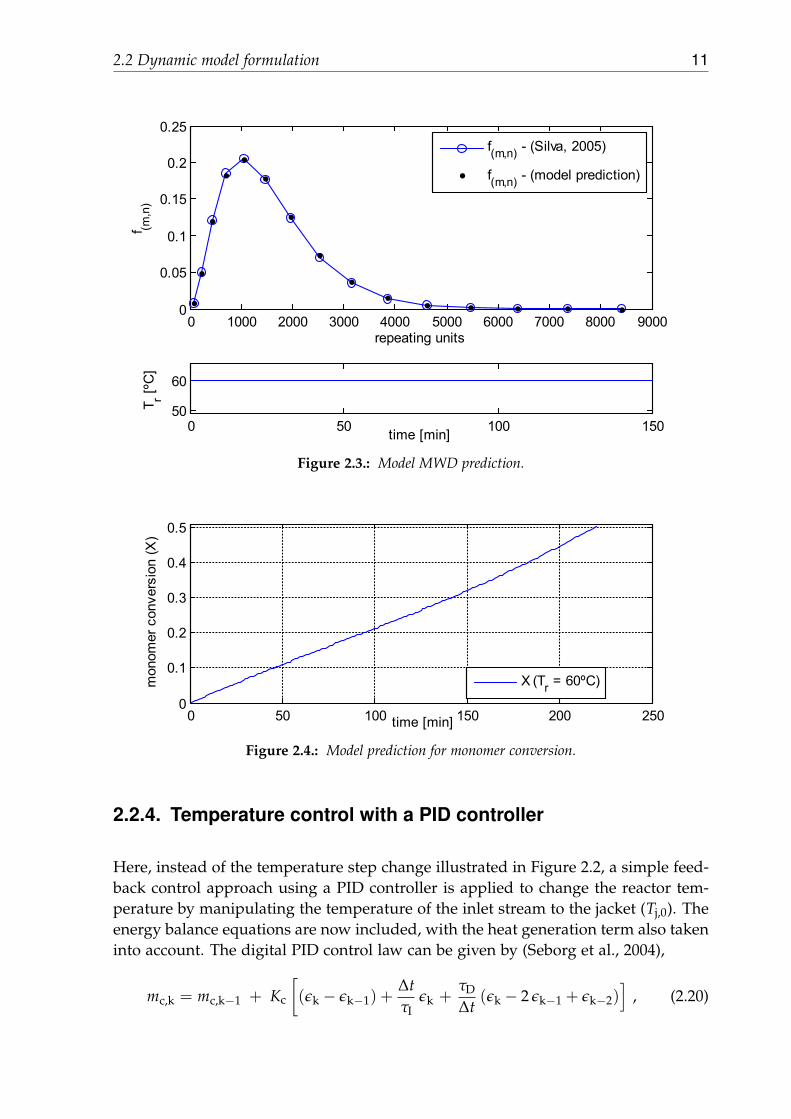
Another test was made to verify the correctness of the numerical implementationof the model. Here the dynamic profiles of monomer conversion, polymer molecularweight averages, and MWD were compared with the simulation results obtained forthis system by Silva (2005). In this case the polymerization is carried out in isother-mal conditions, with a constant reactor temperature of 60 ◦C. Figure 2.3 shows agood agreement between the polymer MWD values obtained by the numerical sim-ulation developed in this work and the results obtained by Silva (2005). Similaritiesare also verified in molecular weight averages and monomer conversion which hasan approximately linear profile (see Table 2.4 and figures 2.4 and 2.5).
2.2 Dynamic model formulation 11
0 1000 2000 3000 4000 5000 6000 7000 8000 90000
0.05
0.1
0.15
0.2
0.25
repeating units
f (m,n
)
0 50 100 15050
60
time [min]
T r [ºC
]f(m,n) - (Silva, 2005)
f(m,n) - (model prediction)
Figure 2.3.: Model MWD prediction.
0 50 100 150 200 2500
0.1
0.2
0.3
0.4
0.5
time [min]
mon
omer
con
vers
ion
(X)
X (Tr = 60ºC)
Figure 2.4.: Model prediction for monomer conversion.
2.2.4. Temperature control with a PID controller
Here, instead of the temperature step change illustrated in Figure 2.2, a simple feed-back control approach using a PID controller is applied to change the reactor tem-perature by manipulating the temperature of the inlet stream to the jacket (Tj,0). Theenergy balance equations are now included, with the heat generation term also takeninto account. The digital PID control law can be given by (Seborg et al., 2004),
mc,k = mc,k−1 + Kc
[(εk − εk−1) +
∆tτI
εk +τD
∆t(εk − 2 εk−1 + εk−2)
], (2.20)
12 Batch Solution Free-radical Polymerization of Methyl Methacrylate (MMA)
0 0.05 0.1 0.15 0.2 0.25 0.3 0.35 0.4 0.45 0.50
50
100
150
monomer conversion (X)
Mn, M
w (k
g/m
ol)
Mn
Mw
Figure 2.5.: Model prediction for molecular weight averages.
Table 2.5.: PID controller parameters: controlled variable - Tr; manipulated variable - Tj,0.
∆t Kc τI τD mc,max mc,min0.2 min 52.5/2 0.93×3 min 0.90/3 min 80.0 ◦C 25.0 ◦C
which is known as the velocity form of the digital PID controller. In (2.20) ∆t is thesampling time period, Kc is the controller proportional gain, τI is the integral time,τD is the derivative time, and mc is the manipulated variable. The error signal at thesampling time k, εk, is defined by:
εk = ysp,k − yk , (2.21)
where ysp,k is the set point and yk is the measured value for the controlled variable.The expression for the digital PID controller in (2.20) can be improved by replacing
the derivate of the error by the derivative of the measured variable. This is done inorder to prevent “derivative kick” phenomena, defined by a immediate large changein the controller output caused by the derivative term when a large step change ismade in the setpoint. Thus, the digital PID control equation becomes:
mc,k = mc,k−1 + Kc
[(εk − εk−1) +
∆tτI
εk −τD
∆t(yk − 2 yk−1 + yk−2)
]. (2.22)
For more details about this subject, see for instance (Seborg et al., 2004).Table 2.5 contains the PID controller parameters, where mcmax and mcmin represent
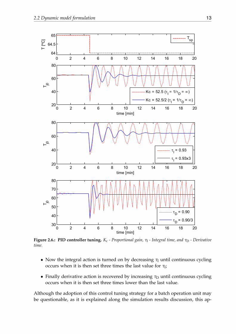
the manipulated variable saturation points. The controller was tuned using the trialand error method explained in Seborg et al. (1989):
• The tuning process starts by eliminating integral and derivative action, that is:τI = ∞ and τD = 0;
• The next step involves Kc tuning by starting from a small value (e.g., 0.5)and slowly increasing it until continuous cycling occurs after a small set pointchange. Kc is then reduced by a factor of two (see Figure 2.6);
2.2 Dynamic model formulation 13
0 2 4 6 8 10 12 14 16 18 2020
40
60
80
time [min]
T j0
Kc = 52.5 (τI = 1/τD = ∞)
Kc = 52.5/2 (τI = 1/τD = ∞)
0 2 4 6 8 10 12 14 16 18 2064
64.5
65
T [º
C]
Tsp
0 2 4 6 8 10 12 14 16 18 2020
40
60
80
time [min]
T j0
τI = 0.93
τI = 0.93x3
0 2 4 6 8 10 12 14 16 18 2030
40
50
60
70
80
time [min]
T j0
τD = 0.90
τD = 0.90/3
Figure 2.6.: PID controller tuning. Kc - Proportional gain, τI - Integral time, and τD - Derivativetime.
• Now the integral action is turned on by decreasing τI until continuous cyclingoccurs when it is then set three times the last value for τI;
• Finally derivative action is recovered by increasing τD until continuous cyclingoccurs when it is then set three times lower than the last value.
Although the adoption of this control tuning strategy for a batch operation unit maybe questionable, as it is explained along the simulation results discussion, this ap-
14 Batch Solution Free-radical Polymerization of Methyl Methacrylate (MMA)
0 20 40 60 80 100 120 140 160 1800
0.2
0.4co
nver
sion
(X)
0 20 40 60 80 100 120 140 160 18050
55
60
65
T r
0 20 40 60 80 100 120 140 160 18050
60
time [min]
T j
monomer conversionstep change in Tsp
Tr
Tr,sp
Figure 2.7.: PID control of reactor temperature in the MMA batch solution polymerization reactor.
75 80 85 90 9520
30
40
50
60
70
time [min]
T j0
Figure 2.8.: Manipulated variable (Tj,0) dynamics under the PID control.
proach is quite acceptable in the context of this particular system. The selection ofthe sampling period, ∆t, was also done by trial and error since there is not any sys-tematic method to do so in batch processes. As observed by Seborg et al. (2004), theselection of the sampling period is more of an art than a science, even for continuousprocesses.
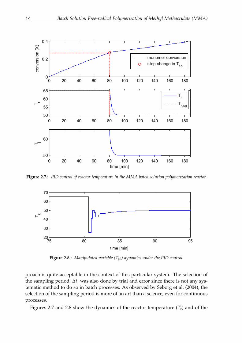
Figures 2.7 and 2.8 show the dynamics of the reactor temperature (Tr) and of the

2.2 Dynamic model formulation 15
0 20 40 60 80 100 120 140 160 180 2000
100
200
time [min]
heat
ratio
Figure 2.9.: Ratio between the heat transfered and the reaction heat.
manipulated variable (Tj,0) under the action of the PID controller. The temperaturecontrol, namely the adopted PID tuning strategy, can be performed in a similarfashion as in a continuous process, due to the fact that the released reaction heat isabout 200 times smaller than the heat transfered between the jacket and the reactionmixture, as it can be observed in Figure 2.9.
One can observe from Figure 2.7 that there is no overshooting in the reactor tem-perature (controlled variable) which is a desirable situation because otherwise a tar-geted final polymer property (e.g., MWD) might not have been achieved. Therefore,it is safe to assume that the controller tuning is acceptable for this particular scenario,which is to decrease the reactor temperature from 65 to 50 ◦C when a 27% monomerconversion is reached.

3. Lab-scale Polymerization Reactor
The batch solution free-radical polymerization of methyl methacrylate (MMA) pro-cess described in Chapter 2 is now applied by simulation in the context of a jacketedlab-scale reactor vessel. As pointed out in Chapter 1, the main goal of this work isto study the thermal dynamics of a lab-scale vessel that can be used for polymeriza-tion experiments. This is motivated by the development of supporting knowledge inorder to predict the thermal dynamic behavior of the lab-scale reactor vessel.
The contents of this chapter is organized as follows. First of all, a brief descriptionof the dimensions and geometry of the lab-scale reactor are given. This is needed todefine namely the heat transfer area. A description of the mathematical model of thelab-scale vessel dynamics is given, and an assessment of its heat transfer capabilitiesis done by simulation in batch operation mode with a water-water and a water-organic fluid system. A correlation to estimate the overall heat transfer coefficientis presented, and three different approximations to model the fluid jacked dynamicsare tested – perfect mixed, plug flow, and lumped jacket model (Luyben, 1989).Results are given with profiles for the main process variables in open-loop mode.Finally, Section 3.2 describes the simulation of the closed-loop control of a batchsolution free-radical polymerization of MMA, where a split-range control strategy isadopted to manipulate both a hot and cold water streams entering the reactor jacket.
Lab-scale reactor characteristicsThe jacketed reactor vessel is supplied by Labglass Ltd and is considered to be thelaboratory standard equipment. The vessel is manufactured from borosilicate with aPTFE tap, has a capacity of 250 ml, an overall height of 225 mm, with the inner andouter diameters of 75 and 105 mm, respectively, and a glass thickness of approxi-mately 2.7 mm. A simplified diagram of the lab-scale reactor is given in Figure 3.1.
3.1. Lab-scale reactor open-loop thermal study
From the application of the energy conservation principle, and after several reason-able and well justified approximations, suitable for liquid systems, the simplifiedenergy balance for a perfectly mixed non-reacting continuous tank system with aconstant inlet flow rate, and a heat transfer rate to or from its surroundings, is of theform (Denn, 1987):
ρVCpdTdt
= ρFCp(Tf − T) + Q , (3.1)
17

18 Lab-scale Polymerization Reactor
Figure 3.1.: Lab-scale reactor.
where ρ is the density of the liquid mixture, V is the tank liquid volume, Cp is theheat capacity of the mixture, T is the temperature of the fluid inside the vessel, Fis the inlet flow rate, Tf is the feed stream temperature, and Q is the heat flux tothe heating/cooling system. For instance, in the particular case of a perfectly mixedjacketed liquid system,
Q = U A (Tj − T) , (3.2)
where U is the overall heat transfer coefficient, A is the heat transfer area, and Tjis the jacket fluid temperature. One emphasizes that (3.1) is obtained under theassumption that the properties ρ and Cp are constant.
Equation (3.1) is applied to both the fluid inside the reactor, and the fluid in thejacket. In the case of the lab-scale reactor operation in batch mode, the first term ofthe right hand side of the equation (3.1) vanishes (i.e., F = 0) in the energy balanceequation related to the mass of the fluid inside the reactor.
3.1.1. Perfectly mixed jacket
In a perfectly mixed cooling or heating jacket model the temperature inside the jacket(Tj) is considered to be spatially constant. This is a good approximation for relativelyhigh flow rates where the thermal fluid temperature does not change significantlyas it goes through the jacket (Luyben, 1989). In this case, and under the assumptionthere are no changes in the composition of the fluid inside the tank, the dynamicmodel of the lab-scale batch vessel is given by
ρrVrCp,rdTr
dt= UA(Tj − Tr) , (3.3a)
ρjVjCp,jdTj
dt= ρjFjCp,j(Tj,0 − Tj) + UA(Tr − Tj) , (3.3b)
where U is the overall heat transfer coefficient, A is the heat transfer area, and thesubscripts r and j refer to the property that belongs to the fluid inside the reactor andinside the jacket, respectively. Also, the model 3.3 is derived under the assumptionthat there are no heat losses.
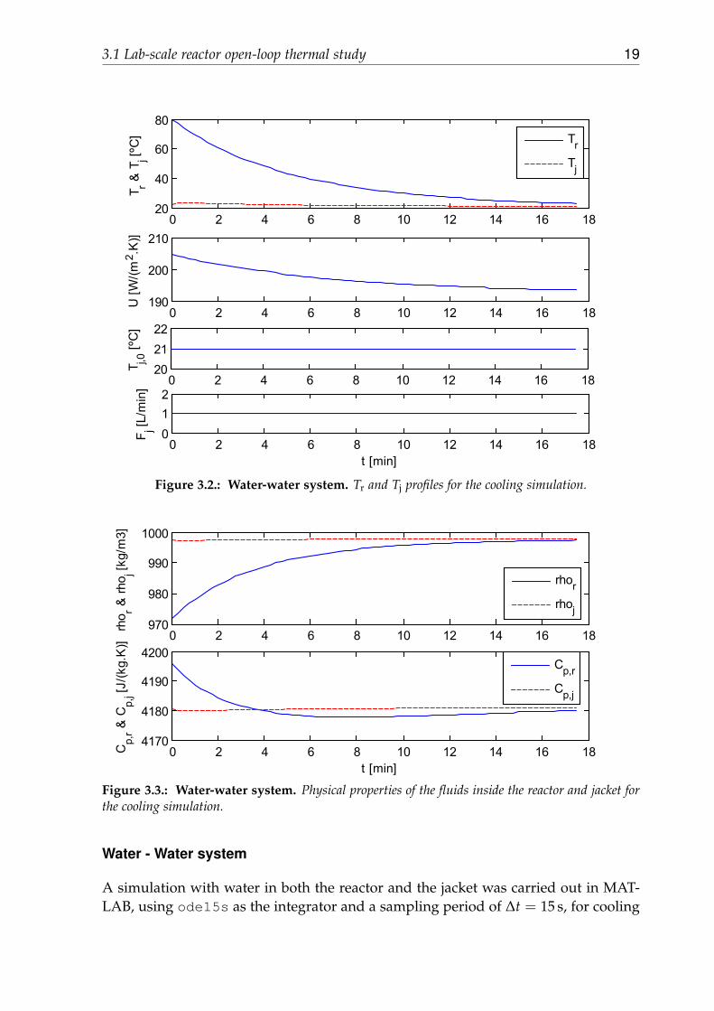
3.1 Lab-scale reactor open-loop thermal study 19
0 2 4 6 8 10 12 14 16 1820
40
60
80T r &
Tj [º
C]
Tr
Tj
0 2 4 6 8 10 12 14 16 18190
200
210
U [W
/(m2 .
K)]
0 2 4 6 8 10 12 14 16 18202122
T j,0 [º
C]
0 2 4 6 8 10 12 14 16 18012
t [min]
F j [L/m
in]
Figure 3.2.: Water-water system. Tr and Tj profiles for the cooling simulation.
0 2 4 6 8 10 12 14 16 18970
980
990
1000
rho r &
rho j [k
g/m
3]
0 2 4 6 8 10 12 14 16 184170
4180
4190
4200
t [min]
Cp,
r & C
p,j [J
/(kg.
K)]
rhor
rhoj
Cp,r
Cp,j
Figure 3.3.: Water-water system. Physical properties of the fluids inside the reactor and jacket forthe cooling simulation.
Water - Water system
A simulation with water in both the reactor and the jacket was carried out in MAT-LAB, using ode15s as the integrator and a sampling period of ∆t = 15 s, for cooling
20 Lab-scale Polymerization Reactor
0 2 4 6 8 10 12 14 16 1820
40
60
80T r &
Tj [º
C]
Tr
Tj
0 2 4 6 8 10 12 14 16 18
190
200
U [W
/(m2 .
K)]
0 2 4 6 8 10 12 14 16 18798081
T j,0 [º
C]
0 2 4 6 8 10 12 14 16 180
12
t [min]
F j [L/m
in]
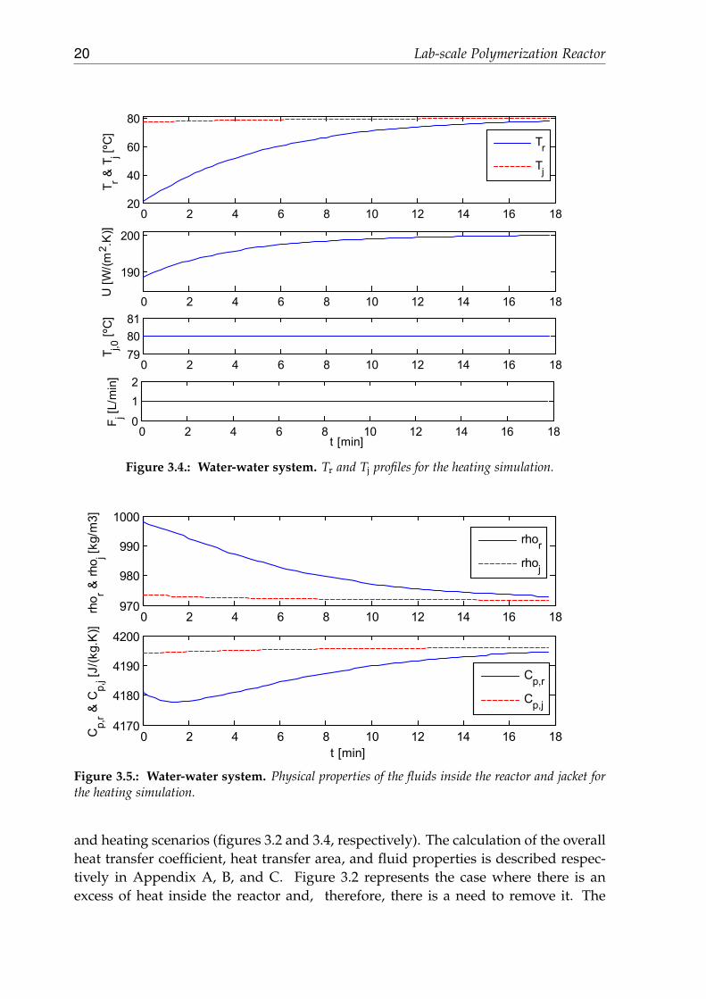
Figure 3.4.: Water-water system. Tr and Tj profiles for the heating simulation.
0 2 4 6 8 10 12 14 16 18970
980
990
1000
rho r &
rho j [k
g/m
3]
0 2 4 6 8 10 12 14 16 184170
4180
4190
4200
t [min]
Cp,
r & C
p,j [J
/(kg.
K)]
rhor
rhoj
Cp,r
Cp,j
Figure 3.5.: Water-water system. Physical properties of the fluids inside the reactor and jacket forthe heating simulation.
and heating scenarios (figures 3.2 and 3.4, respectively). The calculation of the overallheat transfer coefficient, heat transfer area, and fluid properties is described respec-tively in Appendix A, B, and C. Figure 3.2 represents the case where there is anexcess of heat inside the reactor and, therefore, there is a need to remove it. The

3.1 Lab-scale reactor open-loop thermal study 21
0 2 4 6 8 10 12 14 16 18
40
60
80T r &
Tj [º
C]
Tr
Tj
0 2 4 6 8 10 12 14 16 18215220225230
U [W
/(m2 .
K)]
0 2 4 6 8 10 12 14 16 1879
80
81
T j,0 [º
C]
0 2 4 6 8 10 12 14 16 180
1
2
t [min]
F j [L/m
in]
Figure 3.6.: Water-organic system. Tr and Tj profiles for the heating simulation.
0 2 4 6 8 10 12 14 16 18800
900
1000
ρ [k
g.m
-3]
ρr
ρj
0 2 4 6 8 10 12 14 16 182000
3000
4000
5000
t [min]
Cp [J
.kg-1
.K-1
]
Cp,r
Cp,j
Figure 3.7.: Water-organic system. Physical properties of the fluids inside the reactor and jacketfor the heating simulation.
reactor was considered to be initially at 80◦C and the cooling water at 21◦C. Theprofiles in figure 3.2 show that the tank system temperature stabilizes after around18 minutes. The stabilization criterion adopted in the algorithm is a change in Tr ofless than 0.1◦C between the temperatures of two successive sampling time instants.
22 Lab-scale Polymerization Reactor
0 2 4 6 8 10 12 14 16 1820
40
60
80T r &
Tj [º
C]
Tr
Tj
0 2 4 6 8 10 12 14 16 18190
200
210
U [W
/(m2 .
K)]
0 2 4 6 8 10 12 14 16 18202122
T j,0 [º
C]
0 2 4 6 8 10 12 14 16 180
1
2
t [min]
F j [L/m
in]
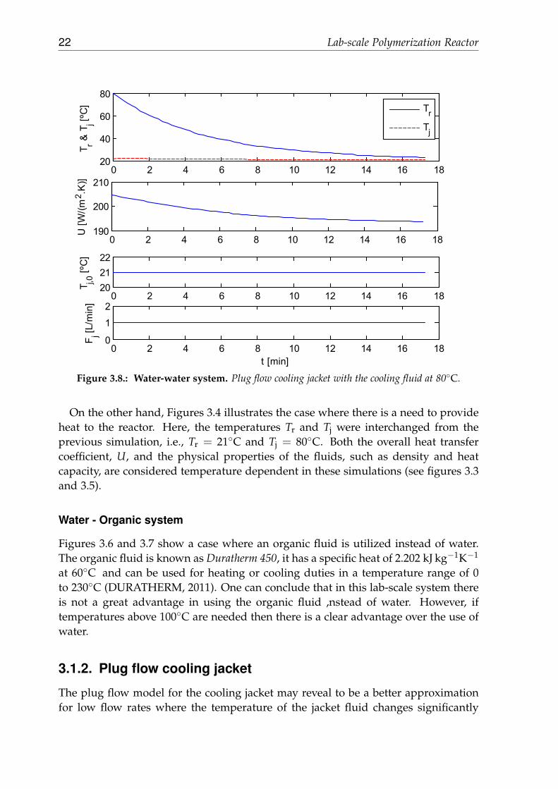
Figure 3.8.: Water-water system. Plug flow cooling jacket with the cooling fluid at 80◦C.
On the other hand, Figures 3.4 illustrates the case where there is a need to provideheat to the reactor. Here, the temperatures Tr and Tj were interchanged from theprevious simulation, i.e., Tr = 21◦C and Tj = 80◦C. Both the overall heat transfercoefficient, U, and the physical properties of the fluids, such as density and heatcapacity, are considered temperature dependent in these simulations (see figures 3.3and 3.5).
Water - Organic system
Figures 3.6 and 3.7 show a case where an organic fluid is utilized instead of water.The organic fluid is known as Duratherm 450, it has a specific heat of 2.202 kJ kg−1K−1
at 60◦C and can be used for heating or cooling duties in a temperature range of 0to 230◦C (DURATHERM, 2011). One can conclude that in this lab-scale system thereis not a great advantage in using the organic fluid ,nstead of water. However, iftemperatures above 100◦C are needed then there is a clear advantage over the use ofwater.
3.1.2. Plug flow cooling jacket
The plug flow model for the cooling jacket may reveal to be a better approximationfor low flow rates where the temperature of the jacket fluid changes significantly
3.1 Lab-scale reactor open-loop thermal study 23
0 2 4 6 8 10 1220
40
60
80T r &
Tj [º
C]
Tr
Tj1
Tj2Tj3
Tj4
0 2 4 6 8 10 12190
200
210
U [W
/(m2 .
K)]
0 2 4 6 8 10 12202122
T j,0 [º
C]
0 2 4 6 8 10 120
12
t [min]
F j [L/m
in]
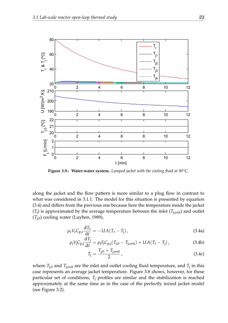
Figure 3.9.: Water-water system. Lumped jacket with the cooling fluid at 80◦C.
along the jacket and the flow pattern is more similar to a plug flow in contrast towhat was considered in 3.1.1. The model for this situation is presented by equation(3.4) and differs from the previous one because here the temperature inside the jacket(Tj) is approximated by the average temperature between the inlet (Tj,exit) and outlet(Tj,0) cooling water (Luyben, 1989),
ρrVrCp,rdTr
dt= −UA(Tr − Tj) , (3.4a)
ρjVjCp,jdTj
dt= ρjFjCp,j(Tj,0 − Tj,exit) + UA(Tr − Tj) , (3.4b)
Tj =Tj,0 + Tj,exit
2, (3.4c)
where Tj,0 and Tj,exit are the inlet and outlet cooling fluid temperature, and Tj in thiscase represents an average jacket temperature. Figure 3.8 shows, however, for theseparticular set of conditions, Tj profiles are similar and the stabilization is reachedapproximately at the same time as in the case of the perfectly mixed jacket model(see Figure 3.2).
24 Lab-scale Polymerization Reactor
0 2 4 6 8 10 1221
21.5
22
22.5
23
23.5T j [º
C]
Tj,1 (Fj,1)
Tj,2 (Fj,1)
Tj,3 (Fj,1)
Tj,4 (Fj,1)
0 2 4 6 8 10 12202224
Tj,1 (Fj,2)
Tj,2 (Fj,2)
Tj,3 (Fj,2)
Tj,4 (Fj,2)
0 2 4 6 8 10 120
5
10
time [min]
F j [L m
in-1
]
Fj,1 = 1 L min-1
Fj,2 = 10 L min-1
Figure 3.10.: Water-water system. Lumped temperatures (Tj,i, i = 1, 4).
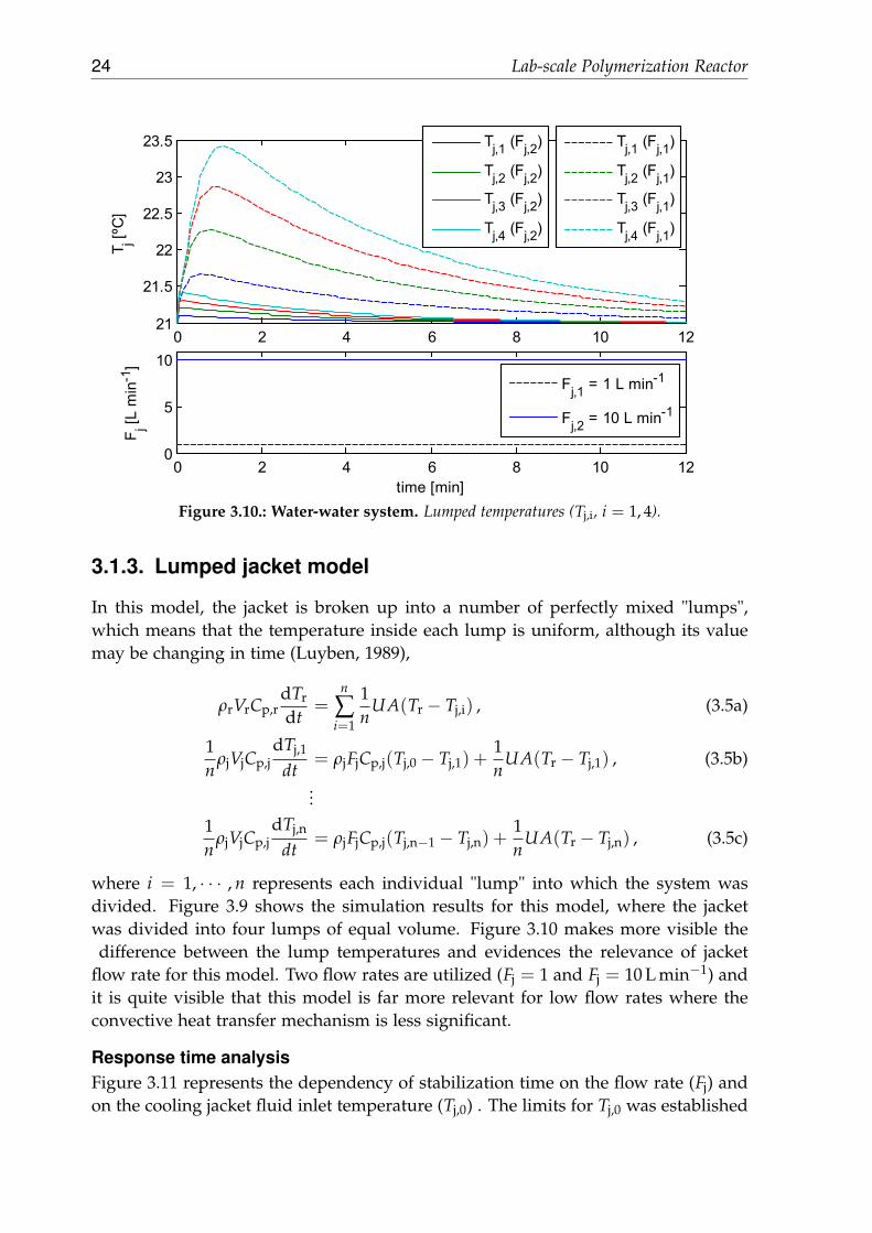
3.1.3. Lumped jacket model
In this model, the jacket is broken up into a number of perfectly mixed "lumps",which means that the temperature inside each lump is uniform, although its valuemay be changing in time (Luyben, 1989),
ρrVrCp,rdTr
dt=
n
∑i=1
1n
UA(Tr − Tj,i) , (3.5a)
1n
ρjVjCp,jdTj,1
dt= ρjFjCp,j(Tj,0 − Tj,1) +
1n
UA(Tr − Tj,1) , (3.5b)
...
1n
ρjVjCp,jdTj,n
dt= ρjFjCp,j(Tj,n−1 − Tj,n) +
1n
UA(Tr − Tj,n) , (3.5c)
where i = 1, · · · , n represents each individual "lump" into which the system wasdivided. Figure 3.9 shows the simulation results for this model, where the jacketwas divided into four lumps of equal volume. Figure 3.10 makes more visible thedifference between the lump temperatures and evidences the relevance of jacket
flow rate for this model. Two flow rates are utilized (Fj = 1 and Fj = 10 L min−1) andit is quite visible that this model is far more relevant for low flow rates where theconvective heat transfer mechanism is less significant.
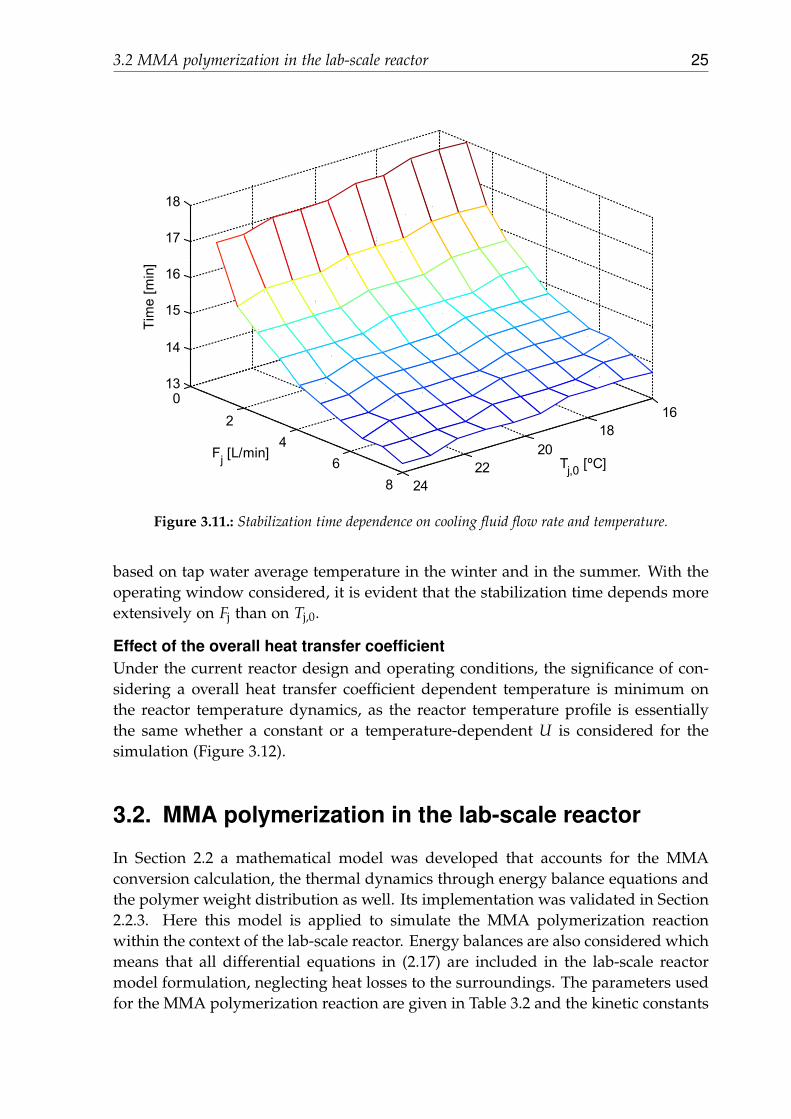
Response time analysisFigure 3.11 represents the dependency of stabilization time on the flow rate (Fj) andon the cooling jacket fluid inlet temperature (Tj,0) . The limits for Tj,0 was established
3.2 MMA polymerization in the lab-scale reactor 25
1618
2022
24
02
46
8
13
14
15
16
17
18
Tj,0 [ºC]Fj [L/min]
Tim
e [m
in]
Figure 3.11.: Stabilization time dependence on cooling fluid flow rate and temperature.
based on tap water average temperature in the winter and in the summer. With theoperating window considered, it is evident that the stabilization time depends moreextensively on Fj than on Tj,0.
Effect of the overall heat transfer coefficientUnder the current reactor design and operating conditions, the significance of con-sidering a overall heat transfer coefficient dependent temperature is minimum onthe reactor temperature dynamics, as the reactor temperature profile is essentiallythe same whether a constant or a temperature-dependent U is considered for thesimulation (Figure 3.12).
3.2. MMA polymerization in the lab-scale reactor
In Section 2.2 a mathematical model was developed that accounts for the MMAconversion calculation, the thermal dynamics through energy balance equations andthe polymer weight distribution as well. Its implementation was validated in Section2.2.3. Here this model is applied to simulate the MMA polymerization reactionwithin the context of the lab-scale reactor. Energy balances are also considered whichmeans that all differential equations in (2.17) are included in the lab-scale reactormodel formulation, neglecting heat losses to the surroundings. The parameters usedfor the MMA polymerization reaction are given in Table 3.2 and the kinetic constants

26 Lab-scale Polymerization Reactor
0 2 4 6 8 10 12 14 16 1820
40
60
80
time [min]
T r [ºC
]
Tr (variable U)
Tr (constant U)
Figure 3.12.: Variable overall heat transfer coefficient (U) significance.
are the same as the ones presented in Section 2.2.3 (see also Appendix D). The initialconditions for the polymerization reaction are given in Table 2.3. The overall heattransfer coefficient is considered to be of 350 W m−2K−1, which is a typical value forjacketed glass vessels (Fletcher, 1981).
3.2.1. Split-range control
A split-range control strategy is implemented in order to maintain the reactor tem-perature (Tr) at the desired values. This type of control, which is essentially a PIDcontrol, is employed when several manipulated variables are used to control a singlecontrolled variable (Seborg et al., 2004). For the current polymerization system, theuse of this type of controller is justified by the necessity of both cooling and heatingthe reactor. Therefore, Tr is controlled by the hot and cold water flow rate in thejacketed reactor, according to the controller signal (mc) which varies from 0 to 100%.The split-range controller is designed such that when mc is less than 50%, the hotstream is turned off while the cold stream is used to control Tr. When mc is greaterthan 50%, it is the other way around. It is necessary to introduce a modificationin the jacket fluid energy balance (2.17h) in order to account for the hot and coldstreams contributions, such that:
dTj
dt=
Fhot
Vj(Thot − Tj) +
Fcold
Vj(Tcold − Tj) +
UA(Tr − Tj)
ρjCp,jVj, (3.6)
where Thot, Tcold, Fhot and Fcold are respectively the temperatures and flow rates ofthe hot and cold streams entering the jacket. There is also a need to define a rangefor the manipulated variables (Fhot and Fcold), as presented in Table 3.1. The values
3.2 MMA polymerization in the lab-scale reactor 27
Table 3.1.: Range for the manipulated variables, Fhot and Fcold.
Fhot / L min−1 Fcold / L min−1
minimum 0 0maximum 10.0 10.0
range = maximum - minimum 10.0 10.0
Table 3.2.: Parameters for the MMA polymerization reaction.
V Vj A Fj Ueff250 mL 170 mL 174 cm2 5.0 L min−1 365.4 J K−1min−1
for the manipulated variables are set according to:
Fhot =
Fhot,range ×mc −mc,split
100−mc,split, if mc −mc,split > 0 ,
0 , if mc −mc,split 6 0 ,(3.7a)
Fcold =
Fcold,range ×mc,split −mc
mc,split, if mc,split −mc > 0 ,
0 , if mc,split −mc 6 0(3.7b)
where Fhot,range and Fcold,range are given in Table 3.1 and mc,split is the point where thesplit occurs. In this study mc,split = 50 %.
3.2.2. Simulation results
Closed-loop response to a temperature setpoint change
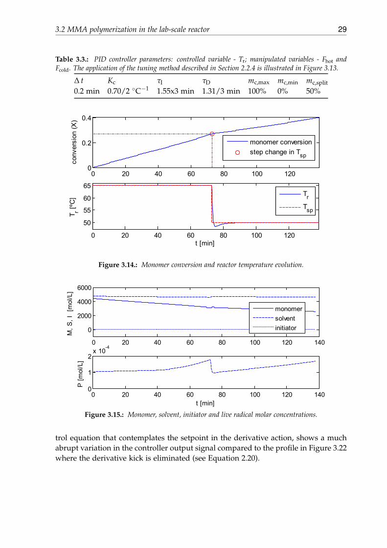
Figures 3.14 to 3.21 show the simulation results for the closed-loop system using thesplit-range control strategy, with a MMA solution free-radical polymerization reac-tion taking place in a laboratory batch reactor. Similarly to the procedure in Section2.2.3, the mixture temperature setpoint is changed from 65 to 50◦C when a 27% con-version is attained. As it can be observed in figures 3.20 and 3.18, this decrease in Tr
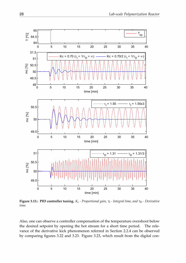
broadens the molecular weight distribution of the resulting polymer and increasesits average molecular weights. However the reactor temperature will not go downinstantaneously, but rather evolves according to heat transfer limitations, under thecontroller actuation (Figure 3.14). The controller was tuned based on the trial anderror method described in section 2.2.4, obtaining the parameters presented in Ta-ble 3.3 and producing the controller command signal in Figure 3.22. Figure 3.13illustrates the application of the mentioned method for the controller tuning.
Figure 3.21 represents the controller output signal in the interval [10, 60]min andit shows that despite of the fact that the system appeared to be in “stead state” atthis period (as suggested by Figure 3.22), the cold flow rate is actually not null. Thecontroller keeps the cold stream valve open just enough to coold down the reactor.
28 Lab-scale Polymerization Reactor
0 5 10 15 20 25 30 35 4049
49.5
50
50.5
51
51.5
mc
[%]
time [min]
0 5 10 15 20 25 30 35 4064
64.5
65T
[ºC
]
Tsp
Kc = 0.70 (τI = 1/τD = ∞) Kc = 0.70/2 (τI = 1/τD = ∞)
0 5 10 15 20 25 30 35 40
49.5
50
50.5
time [min]
mc
[%]
τI = 1.55 τI = 1.55x3
0 5 10 15 20 25 30 35 40
49.5
50
50.5
51
mc
[%]
time [min]
τD = 1.31 τD = 1.31/3
Figure 3.13.: PID controller tuning. Kc - Proportional gain, τI - Integral time, and τD - Derivativetime.
Also, one can observe a controller compensation of the temperature overshoot belowthe desired setpoint by opening the hot stream for a short time period. The rele-vance of the derivative kick phenomenon referred in Section 2.2.4 can be observedby comparing figures 3.22 and 3.23. Figure 3.23, which result from the digital con-
3.2 MMA polymerization in the lab-scale reactor 29
Table 3.3.: PID controller parameters: controlled variable - Tr; manipulated variables - Fhot andFcold. The application of the tuning method described in Section 2.2.4 is illustrated in Figure 3.13.
∆ t Kc τI τD mc,max mc,min mc,split
0.2 min 0.70/2 ◦C−1 1.55x3 min 1.31/3 min 100% 0% 50%
0 20 40 60 80 100 1200
0.2
0.4
conv
ersi
on (X
)
0 20 40 60 80 100 120
50
55
60
65
t [min]
T r [ºC
]
monomer conversionstep change in Tsp
Tr
Tsp
Figure 3.14.: Monomer conversion and reactor temperature evolution.
0 20 40 60 80 100 120 140
0
2000
4000
6000
M, S
, I [
mol
/L]
0 20 40 60 80 100 120 1400
1
2x 10
-4
t [min]
P [m
ol/L
]
monomersolventinitiator
Figure 3.15.: Monomer, solvent, initiator and live radical molar concentrations.
trol equation that contemplates the setpoint in the derivative action, shows a muchabrupt variation in the controller output signal compared to the profile in Figure 3.22where the derivative kick is eliminated (see Equation 2.20).

30 Lab-scale Polymerization Reactor
0 20 40 60 80 100 120 1400.8
1
1.2w
i [%]
0 20 40 60 80 100 120 14048.184
48.186
48.188
t [min]
ws [%
]
Figure 3.16.: Mass fraction of the solvent and the initiator.
0 20 40 60 80 100 120 1400
0.5
1x 10
-3
λ 0
0 20 40 60 80 100 120 1400
0.5
λ 1
0 20 40 60 80 100 120 1400
500
1000
t [min]
λ 2
Figure 3.17.: Molecular weight moments.
0 20 40 60 80 100 120 1400
100
200
t [min]
Mn,
Mw
[kg/
mol
]
0 0.05 0.1 0.15 0.2 0.25 0.3 0.35 0.40
100
200
X
Mn,
Mw
(kg/
mol
)
MnMw
MnMw
Figure 3.18.: Number and weight average molecular weights.

3.2 MMA polymerization in the lab-scale reactor 31
0 1000 2000 3000 4000 5000 6000 7000 8000 90000
0.05
0.1
0.15
0.2
repeating units
f (m,n
)
Figure 3.19.: Molecular weight distribution at the final instant of the reaction.
0
50
100
150 0 2000 4000 6000 8000 10000
0
0.05
0.1
0.15
0.2
0.25
repeating units
time [min]
f (m,n
)
Figure 3.20.: Evolution of the molecular weight distribution during the reaction time.

32 Lab-scale Polymerization Reactor
10 15 20 25 30 35 40 45 50 55 60
50
100
tem
pera
ture
[ºC
]
Tj
Thot
Tcold
10 15 20 25 30 35 40 45 50 55 6005
1015
x 10-5
flow
rate
[L/m
in]
Fhot
Fcold
10 15 20 25 30 35 40 45 50 55 6049.998449.998649.9988
time [min]
mc
[%]
Figure 3.21.: Jacket temperature (Tj), hot and cold fluid flow rate in the jacket (Thot = 85◦C andTcold = 25◦C) and controller command signal (mc) in the interval t = [10, 60]min.
60 65 70 75 80 85 9020
4060
80100
tem
pera
ture
[ºC
]
Tj
Thot
Tcold
60 65 70 75 80 85 900
1
2
flow
rate
[L/m
in]
Fhot
Fcold
60 65 70 75 80 85 90
40
50
60
time [min]
mc
[%]
Figure 3.22.: Jacket temperature (Tj), hot and cold fluid flow rate in the jacket (Thot = 85◦C andTcold = 25◦C) and controller command signal (mc) profiles.

3.2 MMA polymerization in the lab-scale reactor 33
60 65 70 75 80 85 9020
40
60
80100
tem
pera
ture
[ºC
]
Tj
ThotTcold
60 65 70 75 80 85 900
2
4
flow
rate
[L/m
in]
Fhot
Fcold
60 65 70 75 80 85 90
20
40
60
time [min]
mc
[%]
Figure 3.23.: Jacket temperature (Tj), hot and cold fluid flow rate in the jacket (Thot = 85◦C andTcold = 25◦C) and controller command signal (mc) profiles with derivative kick.

4. Conclusions
A mathematical model based on the work of Crowley and Choi (1997b), for MMAsolution polymerization, occurring in a batch laboratory reactor is presented. Themodel incorporates energy balance equations as well as a method for the MWD cal-culation. The simulations involve a thermal study of the lab-scale reactor in Section3.1, validation of the model implementation in Section 2.2.3 and, finally, simulationof MMA polymerization occurring in the laboratory reactor (Section 3.2). The sim-ulations performed in this study for the laboratory reactor will be useful when thereactor is installed, since thermal responsiveness data are available in this work forseveral scenarios, allowing good insight of the reactor thermal behavior. The threemodels considered for the jacket, namely, perfectly mixed, plug flow and lumpedcooling jacket, are equivalent in terms of thermal dynamics, except for low jacketflow rates where the lumped cooling jacket model suggests a significant gradientin temperature along the jacket (see Section 3.1.3). With the MMA polymerizationmodel is also presented, from which conversion and molecular weight distributionare determined. The model takes into consideration the gel effect discussed in Sec-tion 2.1 and the heat of reaction as well. The performed simulations may be used tocontrol the reactor temperature according to a predetermined trajectory that leads tothe desired polymer properties.
The thermal study results, from Section 3.1, denote that it takes around 18 minto heat the lab-scale reactor from 21 to 80◦C or to cool it down from 80 to 21◦C.Nevertheless, this is an approximate result as the heat losses to the exterior are ne-glected and the fluid inside the reactor is water that has different thermodynamicproperties than the MMA reaction mixture. A good mixture can be achieved as thereactor has a small size (250 mL capacity), promoting a good heat transfer betweenthe fluids in the reactor and in the jacket, and making the perfectly mixed modela suitable one for the system. However, the results cannot be directly transposedto a geometrically similar industrial scale reactor, as the relative importance of thetransport phenomena may be different from one scale to another, as pointed out byFaísca (2002).
4.1. Future work
The computational framework developed in this work shows that one can track thesetpoint for the reactor temperature and predict the MWD and monomer conversionprofiles, for a specific time horizon. However, it would be interesting to developnonlinear model predictive control based methodologies to determine the optimal
35
36 Conclusions
reactor temperature setpoints in order to target desired MWD and monomer conver-sion, and also to minimize the reaction time, as demonstrated by Silva and Oliveira(2002). Also, the modeling study must be extended to include the effect of the ther-mal capacitance of the total mass of glass of which the lab-scale reactor is madeof. Regarding the upcoming perspective of performing polymerization experimentswith this reactor, it is of paramount importance to assess the instrumentation andequipment needs to fit the reactor in order to control the reactor temperature and toensure its safety.
Bibliography
Adebekun, D. K. and Schork, F. J. (1989). Continuous solution polymerization reactorcontrol. 1. nonlinear reference control of methyl methacrylate polymerization. Ind.Eng. Chem. Res., 28(9):1308–1324.
Arora, P., Jain, R., Mathur, K., Sharma, A., and Gupta, A. (2010). Synthesis of poly-methyl methacrylate (pmma) by batch emulsion polymerization. African Journal ofPure and Applied Chemistry, 4(8):152–157.
Cao, E. (2009). Heat Transfer in Process Engineering. McGraw-Hill.
Crowley, T. J. and Choi, K. Y. (1997a). Calculation of molecular weight distributionfrom molecular weight moments in free radical polymerization. Ind. Eng. Chem.Res., 36(5):1419–1423.
Crowley, T. J. and Choi, K. Y. (1997b). Discrete optimal control of molecular weightdistribution in a batch free radical polymerization process. Ind. Eng. Chem. Res.,36(9):3676–3684.
Crowley, T. J. and Choi, K. Y. (1998). Experimental studies on optimal molecularweight distribution control in a batch-free radical polymerization process. ChemicalEngineering Science, 53(15):2769–2790.
Curteanu, S., Bulacovschi, V., and Lisa, C. (1998). Free radical polymerization ofmethyl methacrylate: Modeling and simulation by moment generating function.Iranian Polymer Journal, 7(4):152–157.
Debab, A., Chergui, N., and Bertrand, J. (2011). An investigation of heat transfer ina mechanically agitated vessel. Journal of applied fluid mechanics, 4(2).
Denn, M. M. (1987). Process modeling. Harlow : Longman Scientific & Technical,Boston, MA.
DURATHERM (2011). Duratherm 450, heat transfer fluid. http://www.heat-transfer-fluid.com/heat-transfer-fluid/duratherm-450, ac-cessed in May 2011.
Ellis, M. F., Taylor, T. W., Gonzalez, V., and Jensen, K. F. (1988). Estimation of themolecular weight distribution in batch polymerization. AIChE, 34(8):1341–1353.
Faísca, N. P. (2002). Polimerização em Suspensão do VCM. Faculdade de Ciências eTecnologia, Universidade de Coimbra.
37

38 Bibliography
Fletcher, P. (1981). Heat transfer coefficients for stirred batch reactor design. TheChemical Engineer, pages 33–37.
Kell, G. S. (1975). Density, Thermal Expansivity, and Compressibility of Liquid Wa-ter from 0 ◦C to 150 ◦C : Correlations and Tables for Atmospheric Pressure andSaturation Reviewed and Expressed on 1968 Temperature Scale. Journal of Chemicaland Engineering Data, 20(1):97–105.
Kranjk, M., Poljansek, I., and Golob, J. (2001). Kinetic modeling of methyl methacry-late free-radical polymerization initiated by tetraphenyl biphosphine. Polymer,42(9):4153–4162.
Luyben, W. L. (1989). Process Modeling, Simulation and Control for Chemical Engineers.McGraw-Hill chemical engineering series, Schaum’s outline series in civil engi-neering. McGraw-Hill, 2nd edition.
McCabe, W. L., Smith, J. C., and Harriott, P. (1993). Unit Operations of ChemicalEngineering. Chemical and Petroleum Engineering Series. McGraw-Hill, New York,N.Y., 5th edition.
Poling, B. E., Thomson, G. H., Friend, D. G., Rowley, R. L., and Wilding, W. V. (2008).Physical and chemical data. In Perry, R. H. and Green, D. W., editors, Perry’sChemical Engineers’ Handbook. McGraw-Hill, USA.
Rantow, F. S. and Soroush, M. (2005). Optimal control of a high-temperature semi-batch solution polymerization reactor. In American Control Conference 2005, Port-land, OR, USA.
Reid, R. C., Prausnitz, J. M., and Poling, B. E. (1987). The Properties of Gases andLiquids. McGraw-Hill, New York, 4th edition.
Schork, F. J., Deshpande, P. B., and Leffew, K. W. (1993). Control of PolymerizationReactors. Marcel Dekker, Inc., 1st edition.
Seborg, D. E., Edgar, T. F., and Mellichamp, D. A. (1989). Process dynamics and control.Wiley series in chemical engineering. Wiley, 1st edition.
Seborg, D. E., Edgar, T. F., and Mellichamp, D. A. (2004). Process dynamics and control.Wiley series in chemical engineering. Wiley, 2nd edition.
Silva, D. C. M. (2005). Controlo Predictivo Não-linear de Processos Químicos - Aplicaçãoa Sistemas de Polimerização Descontínuos. PhD thesis, Faculdade de Ciências e Tec-nologia, Universidade de Coimbra, Coimbra, Portugal.
Silva, D. C. M. and Oliveira, N. M. C. (2002). Optimization and nonlinear modelpredictive control of batch polymerization systems. Computers and Chemical Engi-neering, 26(4-5):649–658.
Bibliography 39
Yamada, B. and Zetterlund, P. B. (2002). General chemistry of radical polymerization.In Matyjaszewski, K. and Davis, T. P., editors, Handbook of Radical Polymerization.John Wiley & Sons, Inc., USA.


Appendices
41


A. Overall heat transfer coefficient
In section 3.1 a thermal study of the lab-scale reactor was done, where the overallheat transfer coefficient needed to be determined. This chapter illustrates how toestimate its value for an agitated jacketed vessel.
A.1. Internal heat transfer coefficient
Equation (A.1) is an empirical correlation (Debab et al., 2011) for the calculation ofhi, where Nu, Re and Pr are the Nusselt, Reynolds and Prandtl numbers, respectively.
Nu = θ10Rθ20e Pθ30
r Vθ40i . (A.1)
Nu =hiDi
k, (A.2a)
Re =ρNd2
µ, (A.2b)
Pr =µCp
k, (A.2c)
Vi =µ
µw, (A.2d)
where Di is the reactor internal diameter, k is the thermal conductivity of the liquidinside the reactor, ρ is the liquid density, N is the impeller rotational speed, d is theimpeller diameter, µ is the fluid dynamic viscosity at the bulk mean temperature, µw
is the liquid dynamic viscosity at the wall temperature and Cp is the liquid specificheat. hi is determined by substituting (A.2) in (A.1)
Table A.1.: The typical values for the empirical correlation constants (Debab et al., 2011).
θ10 θ20 θ30 θ400.54 2/3 1/3 0.14
43

44 Overall heat transfer coefficient
A.2. External heat transfer coefficient calculation
The heat transfer coefficient in the jacket side can be determined by equation (A.3)(Cao (2009))
hoDH
k= 1.86(RePr
DH
L)
0.33(
µ
µw)
0.14, (A.3)
where DH is the hydraulic diameter given by
DH = 4RH , (A.4)
with L the reactor height (h1 from figure B.1) and RH the ratio between the jacket fluidflow area and the internal tube perimeter. In this case, the internal tube correspondsto the reaction vessel. The Reynolds number for this case is given by equation (A.5),while for Pr calculation the equation (A.2c) still remains valid.
Re =ρuDH
µ. (A.5)
A.3. Overall heat transfer coefficient
The overall heat transfer coefficient based on the internal area (Ui) can be determinedby equation (A.6) (McCabe et al., 1993).
1Ui
=1hi
+xw
km
Di
D̄L+
1ho
Di
Do, (A.6)
where xw is the wall thickness, km is the wall thermal conductivity and D̄L is thelogarithmic mean of the internal and external diameter, given by:
D̄L =Di − Do
log(Di/Do). (A.7)

B. Heat transfer area
Figure B.1.: Representation of the lab-scale polymerization reactor.
The heat transfer area is given by:
A = AL + AB , (B.1)
where AL is the lateral surface area and AB is the base surface area. AL is given by
AL = πDih1 , (B.2)
while AB is approximated by a cone lateral surface area.
AB = π r s where s =√
r2 + h42 . (B.3)
The values of Di, h1 and h4, are given in Table B.1. Therefore, the heat transfer areais:
A =(
π × 75.0× 53.5 + π × 37.5×(√
37.52 + 15.52))
mm2 = 174 cm2 . (B.4)
Table B.1.: Lab-scale reactor dimensions.
Di h1 h475.0 mm 53.5 mm 15.5 mm
45


C. Physical properties of fluids
The information provided here are about thermophysic properties needed for thesimulations in sections 2.2.3, 2.2.4, 3.1 and 3.2. The molecular weight of the polymer-ization reagents are given in table C.1.
C.1. Water
C.1.1. Heat capacity
The water heat capacity in J kg−1K−1 is given by equation C.1, with [T] = ◦C (Reidet al., 1987).
Cp(T) = 4185.5
(0.996185 + 2.874× 10⁻⁴
(T + 100
100
)5.26
+
0.011160× 10−0.036T)
.
(C.1)
C.1.2. Density
Equation (C.2) gives the water density in kg m−3 for a temperature range from 0 to150◦C at atmospheric pressure, according to Kell (1975).
ρ(T) =(
999.83952 + 16.945176T − 7.9870401× 10⁻³T2−
46.170461× 10⁻⁶T3 + 105.56302× 10⁻⁹T4−
280.54253× 10⁻¹²T5)/(
1 + 16.879850× 10⁻³T)
.
(C.2)
Table C.1.: Molecular weight of monomer (methyl methacrylate), solvent (Ethyl acetate) and initiator(2,2’-azobis(2-methylbutanenitrile)) (Ellis et al. (1988)).
compound MMA ethyl acetate 2,2’-azobis(2-methylbutanenitrile)[M] = g mol−1 100.12 88.10 192.00
47

48 Physical properties of fluids
C.1.3. Viscosity
The water dynamic viscosity, [µ] = Pa s, can be calculated from equation (C.3) (Reidet al. (1987)), with [T] = ◦C.
µ(T) = 10−3 × exp(−24.71 + 4209
1T + 273.15
+ 0.04527(T + 273.15)−
3.376× 10⁻⁵(T + 273.15)2)
.(C.3)
C.1.4. Thermal conductivity
According to Poling et al. (2008), the water thermal conductivity, [k] = W m−1K−1,is given by equation (C.4), with [T] = ◦C.
k(T) = −0.432 + 0.0057255× (T + 273.15)− 0.000008078× (T + 273.15)2+
1.861× 10−09 × (T + 273.15)3 .(C.4)
C.2. Ethyl acetate
C.2.1. Heat capacity
From the National Institute of Standards and Technology (NIST) database, the solventheat capacity was found to be
Cp,s = 170.59 (J mol−1K−1) . (C.5)
C.2.2. Density
ρs = 925− 1.237(T − 273.15) (kg m−3) , (C.6)
with [T] = ◦C (Ellis/etal:1988).
C.3. Methyl methacrylate (MMA)
C.3.1. Heat capacity
Cp,m = 114.1 + 6.8299T (J kg−1K−1) , (C.7)
with [T] = ◦C (NIST).
C.3.2. Density
ρm = 965.4− 1.09(T − 273.15)− 9.7× 10⁻⁴(T − 273.15)2 (kg m−3) , (C.8)
with [T] = ◦C (Ellis et al., 1988).

C.4 Poly(methyl methacrylate) (PMMA) 49
C.4. Poly(methyl methacrylate) (PMMA)
C.4.1. Heat capacity
Cp,p = (0.265 + 1.39× 10⁻³T)4.184× 10³ (J kg−1K−1) , (C.9)
with [T] = ◦C (NIST).
C.4.2. Density
ρp =ρm
0.754− 9× 10⁻⁴(T − 273.15)(kg m−3) , (C.10)
with [T] = ◦C and ρm given by equation (C.8) (Ellis et al., 1988).


D. Kinetic Parameters
Table D.1 contains the kinetic parameters for the MMA solution polymerization, withkd being the initiator decomposition rate constant, kp the propagation rate constant,kfm the chain transfer to monomer rate constant, kfs the chain transfer to solvent rateconstant and ktd,0 disproportionation termination rate constant.
Gel effectThe following correlation enables the inclusion of the gel effect into the dispropor-tionation termination rate constant, as described in Crowley and Choi (1997b). Forthat purpose, the free and critical free volumes must be calculated from the followingexpressions:
vf = 0.025 + 0.001(T − 167)φm + 0.001(T − 181)φs + 0.00048(T − 387)φp , (D.1a)
vfcr = 0.186− 2.96× 10⁻⁴(T − 273.16) . (D.1b)
gt1 = 0.10575exp(17.15vf − 0.01715(T − 273.16)) , (D.2a)
gt2 = 2.3× 10⁻⁶exp(75vf) . (D.2b)
gt = 0.5 ((gt1 − gt2) tanh (150 (vf − vfcr)) + gt1 + gt2) , (D.3)
ktd = gt × ktd,0 , (D.4)
with φm, φs and φp the monomer, solvent and polymer volume fractions, vf and vfcrthe free volume and the critical free volume, respectively, gt the gel effect parameterand [T] = K.
Heat of MMA polymerizationAccording to Adebekun and Schork (1989), MMA polymerization reaction is exother-mic, with a heat of reaction (∆H) of -13.8 kcal/mol.
51
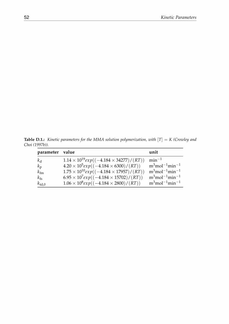
52 Kinetic Parameters
Table D.1.: Kinetic parameters for the MMA solution polymerization, with [T] = K (Crowley andChoi (1997b)).
parameter value unit
kd 1.14× 10¹⁹exp((−4.184× 34277)/(RT)) min−1
kp 4.20× 10⁵exp((−4.184× 6300)/(RT)) m3mol−1min−1
kfm 1.75× 10¹⁰exp((−4.184× 17957)/(RT)) m3mol−1min−1
kfs 6.95× 10⁷exp((−4.184× 15702)/(RT)) m3mol−1min−1
ktd,0 1.06× 10⁸exp((−4.184× 2800)/(RT)) m3mol−1min−1
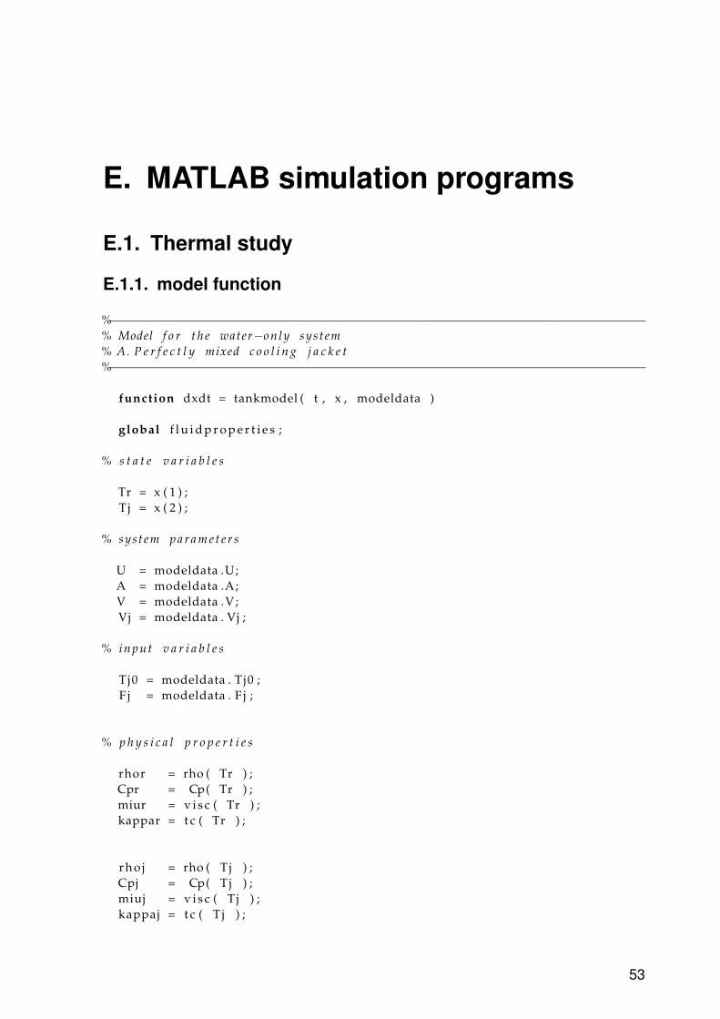
E. MATLAB simulation programs
E.1. Thermal study
E.1.1. model function
%−−−−−−−−−−−−−−−−−−−−−−−−−−−−−−−−−−−−−−−−−−−−−−−−−−−−−−−−−−−−−−−−−−−−−−−−−−% Model f o r t h e water−on ly sys t em% A. P e r f e c t l y mixed c o o l i n g j a c k e t%−−−−−−−−−−−−−−−−−−−−−−−−−−−−−−−−−−−−−−−−−−−−−−−−−−−−−−−−−−−−−−−−−−−−−−−−−−
function dxdt = tankmodel ( t , x , modeldata )
global f l u i d p r o p e r t i e s ;
% s t a t e v a r i a b l e s
Tr = x ( 1 ) ;T j = x ( 2 ) ;
% system p a r a m e t e r s
U = modeldata .U;A = modeldata .A;V = modeldata .V;Vj = modeldata . Vj ;
% i n p u t v a r i a b l e s
Tj0 = modeldata . T j0 ;F j = modeldata . F j ;
% p h y s i c a l p r o p e r t i e s
rhor = rho ( Tr ) ;Cpr = Cp( Tr ) ;miur = v i s c ( Tr ) ;kappar = t c ( Tr ) ;
r h o j = rho ( T j ) ;Cpj = Cp( T j ) ;miuj = v i s c ( T j ) ;kappaj = t c ( T j ) ;
53

54 MATLAB simulation programs
% p a s s t h i s i n f o t o t h e main program
f l u i d p r o p e r t i e s . r h o j = r h o j ;f l u i d p r o p e r t i e s . rhor = rhor ;f l u i d p r o p e r t i e s . Cpj = Cpj ;f l u i d p r o p e r t i e s . Cpr = Cpr ;f l u i d p r o p e r t i e s . miuj = miuj ;f l u i d p r o p e r t i e s . miur = miur ;f l u i d p r o p e r t i e s . kappaj = kappaj ;f l u i d p r o p e r t i e s . kappar = kappar ;
% ene rgy b a l a n c e s
h e a t t r a n s f e r = U ∗ A ∗ ( T j − Tr ) ;
dTrdt = h e a t t r a n s f e r / ( rhor ∗ Cpr ∗ V ) ;
dTjdt = ( F j ∗ r h o j ∗ Cpj ∗ ( T j0 − Tj ) − h e a t t r a n s f e r ) / ( r h o j ∗ Cpj ∗ Vj ) ;
dxdt = [ dTrdt ; dTjdt ] ;
end
%−−−−−−−−−−−−−−−−−−−−−−−−−−−−−−−−−−−−−−−−−−−−−−−−−−−−−−−−−−−−−−−−−−−−−−−−−−% p h y s i c a l p r o p e r t i e s o f wat e r%−−−−−−−−−−−−−−−−−−−−−−−−−−−−−−−−−−−−−−−−−−−−−−−−−−−−−−−−−−−−−−−−−−−−−−−−−−
function C = Cp( T ) %[ J / ( kg∗K ) ] h e a t c a p a c i t yC = 4 1 8 5 . 5∗ ( 0 . 9 9 6 1 8 5 + 2 .874 e−4∗((T+100)/100) .^5 .26+0 .011160∗10 .^( −0 .036∗T ) ) ;
end
function D = rho ( T ) %[ kg /m^3] d e n s i t yD = (999 .83952+16 .945176∗T−7.9870401e−3∗T.^2 . . .
−46.170461∗10^−6∗T.^3 + 105.56302∗10^−9∗T.^4 . . .−280.54253∗10^−12∗T.^5)/(1+16.879850∗10^−3∗T ) ;
end
function miu = v i s c ( T ) %[ Pa∗ s ] dynamic v i s c o s i t ymiu = 1e−3∗exp (−24.71 + 4 2 0 9∗ ( 1 . / ( T + 2 7 3 . 1 5 ) ) + 0 . 0 4 5 2 7∗ (T + 2 7 3 . 1 5 ) . . .
− 3.376∗10^−5∗(T + 2 7 3 . 1 5 ) . ^ 2 ) ;end
function k = t c ( T ) %[W/ (m∗K ) ] t h e r m a l c o n d u c t i v i t yk = −0.432 + 0 . 0 0 5 7 2 5 5∗ (T+273 .15 ) − 0 .000008078∗ (T+ 2 7 3 . 1 5 ) . ^ 2 + . . .
1 . 861E−09∗(T + 2 7 3 . 1 5 ) . ^ 3 ;end
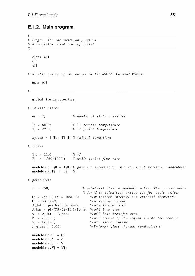
E.1 Thermal study 55
E.1.2. Main program
%−−−−−−−−−−−−−−−−−−−−−−−−−−−−−−−−−−−−−−−−−−−−−−−−−−−−−−−−−−−−−−−−−−−−−−−−−−% Program f o r t h e water−on ly sys t em% A. P e r f e c t l y mixed c o o l i n g j a c k e t%−−−−−−−−−−−−−−−−−−−−−−−−−−−−−−−−−−−−−−−−−−−−−−−−−−−−−−−−−−−−−−−−−−−−−−−−−−
c l e a r a l lc l cc l f
% d i s a b l e pag ing o f t h e o u tp ut in t h e MATLAB Command Window
more o f f
%−−−−−−−−−−−−−−−−−−−−−−−−−−−−−−−−−−−−−−−−−−−−−−−−−−−−−−−−−−−−−−−−−−−−−−−−−
global f l u i d p r o p e r t i e s ;
% i n i t i a l s t a t e s
ns = 2 ; % number o f s t a t e v a r i a b l e s
Tr = 8 0 . 0 ; % oC r e a c t o r t e m p e r a t u r eTj = 2 2 . 0 ; % oC j a c k e t t e m p e r a t u r e
xplant = [ Tr ; T j ] ; % i n i t i a l c o n d i t i o n s
% i n p u t s
Tj0 = 2 1 . 0 ; % oCF j = 1/60/1000 . ; % m^3/ s j a c k e t f l o w r a t e
modeldata . T j0 = Tj0 ; % p a s s t h e i n f o r m a t i o n i n t o t h e i n p u t v a r i a b l e " m o d e l d a t a "modeldata . F j = F j ; %
% p a r a m e t e r s
U = 2 5 0 ; % W/ (m^2∗K) ( J u s t a s y m b o l i c v a l u e . The c o r r e c t v a l u e% f o r U i s c a l c u l a t e d i n s i d e t h e f o r−c y c l e b e l l o w
Di = 75e−3; D0 = 105e−3; % m r e a c t o r i n t e r n a l and e x t e r n a l d i a m e t e r sL1 = 5 3 . 5 e−3; % m r e a c t o r h e i g h tA_lat = pi∗Di ∗53 .5∗1 e−3; % m^2 l a t e r a l a r e aA_bas = pi ∗ ( 75 /2)∗40 . 6∗1 e−6; % m^2 b a s e a r e aA = A_lat + A_bas ; % m^2 h e a t t r a n s f e r a r e aV = 250e−6; % m^3 volume o f t h e l i q u i d i n s i d e t h e r e a c t o rVj = 170e−6; % m^3 j a c k e t volumek_glass = 1 . 0 5 ; % W/ (m∗K) g l a s s t h e r m a l c o n d u c t i v i t y
modeldata .U = U;modeldata .A = A;modeldata .V = V;modeldata . Vj = Vj ;
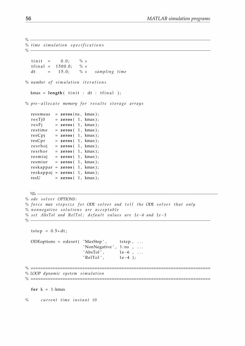
56 MATLAB simulation programs
%−−−−−−−−−−−−−−−−−−−−−−−−−−−−−−−−−−−−−−−−−−−−−−−−−−−−−−−−−−−−−−−−−−−−−−−−−% time s i m u l a t i o n s p e c i f i c a t i o n s%−−−−−−−−−−−−−−−−−−−−−−−−−−−−−−−−−−−−−−−−−−−−−−−−−−−−−−−−−−−−−−−−−−−−−−−−−
t i n i t = 0 . 0 ; % st f i n a l = 1 5 0 0 . 0 ; % sdt = 1 5 . 0 ; % s sampl ing t ime
% number o f s i m u l a t i o n i t e r a t i o n s
kmax = length ( t i n i t : dt : t f i n a l ) ;
% pre−a l l o c a t e memory f o r r e s u l t s s t o r a g e a r r a y s
resxmeas = zeros ( ns , kmax ) ;r e s T j 0 = zeros ( 1 , kmax ) ;r e s F j = zeros ( 1 , kmax ) ;res t ime = zeros ( 1 , kmax ) ;resCpj = zeros ( 1 , kmax ) ;resCpr = zeros ( 1 , kmax ) ;r e s r h o j = zeros ( 1 , kmax ) ;res rhor = zeros ( 1 , kmax ) ;resmiuj = zeros ( 1 , kmax ) ;resmiur = zeros ( 1 , kmax ) ;reskappar = zeros ( 1 , kmax ) ;reskappaj = zeros ( 1 , kmax ) ;resU = zeros ( 1 , kmax ) ;
%%−−−−−−−−−−−−−−−−−−−−−−−−−−−−−−−−−−−−−−−−−−−−−−−−−−−−−−−−−−−−−−−−−−−−−−−−−% ode s o l v e r OPTIONS :% f o r c e max s t e p s i z e f o r ODE s o l v e r and t e l l t h e ODE s o l v e r t h a t on ly% n o n n e g a t i v e s o l u t i o n s a r e a c c e p t a b l e% s e t AbsTol and R e l T o l ; d e f a u l t v a l u e s a r e 1e−6 and 1e−3%−−−−−−−−−−−−−−−−−−−−−−−−−−−−−−−−−−−−−−−−−−−−−−−−−−−−−−−−−−−−−−−−−−−−−−−−−
t s t e p = 0 . 5∗ dt ;
ODEoptions = odeset ( ’ MaxStep ’ , t s tep , . . .’ NonNegative ’ , 1 : ns , . . .’ AbsTol ’ , 1e−6 , . . .’ RelTol ’ , 1e−4 ) ;
% =========================================================================% LOOP dynamic sys t em s i m u l a t i o n% =========================================================================
for k = 1 : kmax
% c u r r e n t t ime i n s t a n t t0
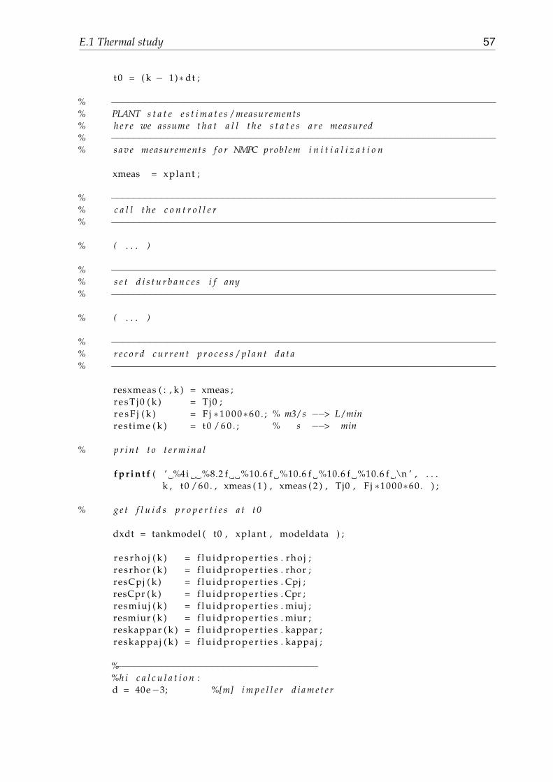
E.1 Thermal study 57
t 0 = ( k − 1)∗ dt ;
% −−−−−−−−−−−−−−−−−−−−−−−−−−−−−−−−−−−−−−−−−−−−−−−−−−−−−−−−−−−−−−−−−−−−−% PLANT s t a t e e s t i m a t e s / measurements% h e r e we assume t h a t a l l t h e s t a t e s a r e measured% −−−−−−−−−−−−−−−−−−−−−−−−−−−−−−−−−−−−−−−−−−−−−−−−−−−−−−−−−−−−−−−−−−−−−% s a v e measurements f o r NMPC prob l em i n i t i a l i z a t i o n
xmeas = xplant ;
% −−−−−−−−−−−−−−−−−−−−−−−−−−−−−−−−−−−−−−−−−−−−−−−−−−−−−−−−−−−−−−−−−−−−−% c a l l t h e c o n t r o l l e r% −−−−−−−−−−−−−−−−−−−−−−−−−−−−−−−−−−−−−−−−−−−−−−−−−−−−−−−−−−−−−−−−−−−−−
% ( . . . )
% −−−−−−−−−−−−−−−−−−−−−−−−−−−−−−−−−−−−−−−−−−−−−−−−−−−−−−−−−−−−−−−−−−−−−% s e t d i s t u r b a n c e s i f any% −−−−−−−−−−−−−−−−−−−−−−−−−−−−−−−−−−−−−−−−−−−−−−−−−−−−−−−−−−−−−−−−−−−−−
% ( . . . )
% −−−−−−−−−−−−−−−−−−−−−−−−−−−−−−−−−−−−−−−−−−−−−−−−−−−−−−−−−−−−−−−−−−−−−% r e c o r d c u r r e n t p r o c e s s / p l a n t d a t a% −−−−−−−−−−−−−−−−−−−−−−−−−−−−−−−−−−−−−−−−−−−−−−−−−−−−−−−−−−−−−−−−−−−−−
resxmeas ( : , k ) = xmeas ;r e s T j 0 ( k ) = Tj0 ;r e s F j ( k ) = F j ∗1 0 0 0∗6 0 . ; % m3 / s −−> L / minres t ime ( k ) = t0 / 6 0 . ; % s −−> min
% p r i n t t o t e r m i n a l
f p r i n t f ( ’ %4i %8.2 f %10.6 f %10.6 f %10.6 f %10.6 f \n ’ , . . .k , t 0 / 6 0 . , xmeas ( 1 ) , xmeas ( 2 ) , Tj0 , F j ∗1000∗60 . ) ;
% g e t f l u i d s p r o p e r t i e s a t t0
dxdt = tankmodel ( t0 , xplant , modeldata ) ;
r e s r h o j ( k ) = f l u i d p r o p e r t i e s . r h o j ;res rhor ( k ) = f l u i d p r o p e r t i e s . rhor ;resCpj ( k ) = f l u i d p r o p e r t i e s . Cpj ;resCpr ( k ) = f l u i d p r o p e r t i e s . Cpr ;resmiuj ( k ) = f l u i d p r o p e r t i e s . miuj ;resmiur ( k ) = f l u i d p r o p e r t i e s . miur ;reskappar ( k ) = f l u i d p r o p e r t i e s . kappar ;reskappaj ( k ) = f l u i d p r o p e r t i e s . kappaj ;
%−−−−−−−−−−−−−−−−−−−−−−−−−−−−−−−−−−−−%h i c a l c u l a t i o n :d = 40e−3; %[m] i m p e l l e r d i a m e t e r
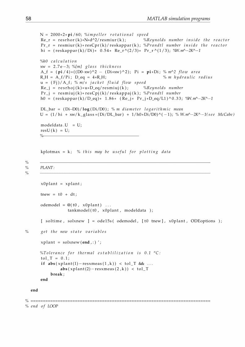
58 MATLAB simulation programs
N = 2000∗2∗pi /60; %i m p e l l e r r o t a t i o n a l s p e e dRe_r = resrhor ( k )∗N∗d^2/resmiur ( k ) ; %Reyno lds number i n s i d e t h e r e a c t o rPr_r = resmiur ( k )∗ resCpr ( k)/ reskappar ( k ) ; %P r a n d t l number i n s i d e t h e r e a c t o rhi = ( reskappar ( k)/ Di )∗ 0 .54∗ Re_r ^(2/3)∗ Pr_r ^ ( 1 / 3 ) ; %W.m̂ −2K^−1
%h0 c a l c u l a t i o nxw = 2 . 7 e−3; %[m] g l a s s t h i c k n e s sA_f = ( pi / 4 )∗ ( (D0−xw)^2 − ( Di+xw) ^ 2 ) ; Pi = pi∗Di ; % m^2 f l o w a r e aR_H = A_f/Pi ; D_eq = 4∗R_H; % m h y d r a u l i c r a d i u su = ( F j )/ A_f ; % m/ s j a c k e t f l u i d f l o w s p e e dRe_j = r e s r h o j ( k )∗u∗D_eq/resmiuj ( k ) ; %Reyno lds numberP r _ j = resmiuj ( k )∗ resCpj ( k)/ reskappaj ( k ) ; %P r a n d t l numberh0 = ( reskappar ( k)/D_eq )∗ 1 .86∗ ( Re_j ∗ P r _ j ∗D_eq/L1 ) ^ 0 . 3 3 ; %W.m̂ −2K^−1
DL_bar = ( Di−D0)/ log ( Di/D0 ) ; % m d i a m e t e r l o g a r i t h m i c meanU = (1/ hi + xw/k_glass ∗ ( Di/DL_bar ) + 1/h0∗Di/D0)^(−1) ; % W.m̂ −2K^−1( s e e McCabe )
modeldata .U = U;resU ( k ) = U;%−−−−−−−−−−−−−−−−−−−−−−−−−−−−−−−−−−−−−−−
kplotmax = k ; % t h i s may be u s e f u l f o r p l o t t i n g d a t a
% −−−−−−−−−−−−−−−−−−−−−−−−−−−−−−−−−−−−−−−−−−−−−−−−−−−−−−−−−−−−−−−−−−−−−% PLANT :% −−−−−−−−−−−−−−−−−−−−−−−−−−−−−−−−−−−−−−−−−−−−−−−−−−−−−−−−−−−−−−−−−−−−−
x0plant = xplant ;
tnew = t0 + dt ;
odemodel = @( t0 , x0plant ) . . .tankmodel ( t0 , x0plant , modeldata ) ;
[ sol t ime , solxnew ] = ode15s ( odemodel , [ t0 tnew ] , x0plant , ODEoptions ) ;
% g e t t h e new s t a t e v a r i a b l e s
xplant = solxnew ( end , : ) ’ ;
%T o l e r a n c e f o r t h e r m a l e s t a b l i l i z a t i o n i s 0 . 1 oC :to l_T = 0 . 1 ;i f abs ( xplant (1)− resxmeas ( 1 , k ) ) < to l_T && . . .
abs ( xplant (2)− resxmeas ( 2 , k ) ) < to l_Tbreak ;
end
end
% =========================================================================% end o f LOOP

E.1 Thermal study 59
% =========================================================================
%% p l o t r e s u l t s
f igure ( 1 )
subplot ( 7 , 1 , 1 : 3 )plot ( res t ime ( 1 : kplotmax ) , resxmeas ( 1 , 1 : kplotmax ) ) ; hold on ;plot ( res t ime ( 1 : kplotmax ) , resxmeas ( 2 , 1 : kplotmax ) , ’ r−− ’ ) ;
%x l a b e l ( ’ t ( min ) ’ )ylabel ( ’ T_r & T_j [ oC ] ’ )legend ( ’ T_r ’ , ’ T_ j ’ )hold o f f
subplot ( 7 , 1 , 4 : 5 )plot ( res t ime ( 1 : kplotmax ) , resU ( 1 : kplotmax ) ) ;xlabel ( ’ t [ min ] ’ )ylabel ( ’U [W/(m^2.K) ] ’ )
subplot ( 7 , 1 , 6 )plot ( res t ime ( 1 : kplotmax ) , r e s T j 0 ( 1 : kplotmax ) ) ; hold on ;
%x l a b e l ( ’ t [ min ] ’ )ylabel ( ’ T_ { j , 0 } [ oC ] ’ )hold o f f
subplot ( 7 , 1 , 7 )s t a i r s ( res t ime ( 1 : kplotmax ) , r e s F j ( 1 : kplotmax ) ) ; hold on ;xlabel ( ’ t [ min ] ’ )ylabel ( ’ F _ j [ L/min ] ’ )hold o f f
f igure ( 2 )
subplot ( 2 , 1 , 1 )plot ( res t ime ( 1 : kplotmax ) , res rhor ( 1 : kplotmax ) ) ; hold on ;plot ( res t ime ( 1 : kplotmax ) , r e s r h o j ( 1 : kplotmax ) , ’ r−− ’ ) ;
%x l a b e l ( ’ t [ min ] ’ )ylabel ( ’ rho_r & rho_ j [ kg/m3] ’ )legend ( ’ rho_r ’ , ’ rho_ j ’ , 4 )hold o f f
subplot ( 2 , 1 , 2 )plot ( res t ime ( 1 : kplotmax ) , resCpr ( 1 : kplotmax ) ) ; hold on ;plot ( res t ime ( 1 : kplotmax ) , resCpj ( 1 : kplotmax ) , ’ r−− ’ ) ;xlabel ( ’ t [ min ] ’ )ylabel ( ’C_ { p , r } & C_ { p , j } [ J /(kg .K) ] ’ )legend ( ’C_ { p , r } ’ , ’C_ { p , j } ’ )
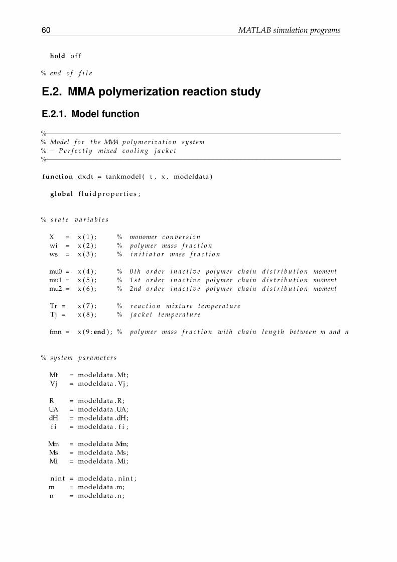
60 MATLAB simulation programs
hold o f f
% end o f f i l e
E.2. MMA polymerization reaction study
E.2.1. Model function
%−−−−−−−−−−−−−−−−−−−−−−−−−−−−−−−−−−−−−−−−−−−−−−−−−−−−−−−−−−−−−−−−−−−−−−−−−−% Model f o r t h e MMA p o l y m e r i z a t i o n sys t em% − P e r f e c t l y mixed c o o l i n g j a c k e t%−−−−−−−−−−−−−−−−−−−−−−−−−−−−−−−−−−−−−−−−−−−−−−−−−−−−−−−−−−−−−−−−−−−−−−−−−−
function dxdt = tankmodel ( t , x , modeldata )
global f l u i d p r o p e r t i e s ;
% s t a t e v a r i a b l e s
X = x ( 1 ) ; % monomer c o n v e r s i o nwi = x ( 2 ) ; % polymer mass f r a c t i o nws = x ( 3 ) ; % i n i t i a t o r mass f r a c t i o n
mu0 = x ( 4 ) ; % 0 th o r d e r i n a c t i v e po lymer c h a i n d i s t r i b u t i o n momentmu1 = x ( 5 ) ; % 1 s t o r d e r i n a c t i v e po lymer c h a i n d i s t r i b u t i o n momentmu2 = x ( 6 ) ; % 2nd o r d e r i n a c t i v e po lymer c h a i n d i s t r i b u t i o n moment
Tr = x ( 7 ) ; % r e a c t i o n mix ture t e m p e r a t u r eTj = x ( 8 ) ; % j a c k e t t e m p e r a t u r e
fmn = x ( 9 : end ) ; % polymer mass f r a c t i o n with c h a i n l e n g t h be tween m and n
% syst em p a r a m e t e r s
Mt = modeldata . Mt ;Vj = modeldata . Vj ;
R = modeldata . R ;UA = modeldata .UA;dH = modeldata .dH;f i = modeldata . f i ;
Mm = modeldata .Mm;Ms = modeldata .Ms ;Mi = modeldata . Mi ;
n in t = modeldata . n in t ;m = modeldata .m;n = modeldata . n ;

E.2 MMA polymerization reaction study 61
wm0 = modeldata .wm0;
% Fj = m o d e l d a t a . F j ;
Fhot = modeldata . Fhot ;Thot = modeldata . Thot ;Fcold = modeldata . Fcold ;Tcold = modeldata . Tcold ;
% p h y s i c a l p r o p e r t i e s
wm = wm0∗ (1 − X ) ;
wp = 1 − ws − wm;
rhom = rho_m ( Tr ) ; rhop = rho_p ( Tr ) ; rhos = rho_s ( Tr ) ; r h o j = rho_ j ( Tr ) ;rhor = wm∗rhom + ws∗ rhos + wp∗rhop ;
Cpm = Cp_m( Tr ) ; Cps = Cp_s ( Tr ) ; Cpp = Cp_p ( Tr ) ;Cpr = wm∗Cpm + ws∗Cps + wp∗Cpp ;Cpj = Cp_j ( T j ) ;
% k i n e t i c p a r a m e t e r s f o r MMA s o l u t i o n p o l y m e r i z a t i o n ( Crowley & Choi , 1997)
TK = Tr + 2 7 3 . 1 5 ; % c o n v e r s i o n from oC t o KRTK = R ∗ TK ;%Crowley & Choi 1997 bkd = 1 . 1 4 ∗ 10^19∗exp ( −4.184∗34277/RTK ) ; % min^−1 i n i t i a t o r d e c o m p o s i t i o nkp = 4 . 2 0 ∗ 10^5 ∗exp ( −4.184∗6300/RTK ) ; % m^ 3 / ( mol . min ) p r o p a g a t i o nkfm = 1 . 7 5 ∗ 10^10∗exp ( −4.184∗17957/RTK ) ; % m^ 3 / ( mol . min ) c h a i n t o monomer t r a n s f e r Crowley & Choi ( 1 9 9 7 )kfs = 6 . 9 5 ∗ 10^7 ∗exp ( −4.184∗15702/RTK ) ; % m^ 3 / ( mol . min ) c h a i n t o s o l v e n t t r a n s f e r r e a c t i o n r a t e c o n s t a n tkt0 = 1 . 0 6 ∗ 10^8 ∗exp ( −4.184∗2800/RTK ) ; % m^ 3 / ( mol . min ) t e r m i n a t i o n r a t e c o n s t a n t
% mixture volume
V = ( wm/rhom + wp/rhop + ws/rhos ) ∗ Mt ; %m^3
% volume f r a c t i o n s o f M, S , P , I
phim = wm ∗ Mt / ( rhom∗V ) ;phip = wp ∗ Mt / ( rhop∗V ) ;phis = 1 − phim − phip ;
% f r e e volume and c r i t i c a l f r e e volume
Vf = 0 .025 + 0 . 0 0 1∗ (TK − 167)∗phim + 0 . 0 0 1∗ (TK − 181)∗ phis + 0 . 0 0 0 4 8∗ (TK − 387)∗phip ;V f c r i = 0 .186 − 2 . 9 6 ∗ 10^−4∗(TK − 2 7 3 . 1 6 ) ;
% g e l e f f e c t p a r a m e t e r
gt1 = 0 .10575 ∗ exp ( 17 .15∗Vf − 0 . 0 1 7 1 5∗ (TK − 2 7 3 . 1 6 ) ) ;

62 MATLAB simulation programs
gt2 = 2 . 3 ∗ 10^−6 ∗ exp ( 75∗Vf ) ;
gt = 0 . 5 ∗ ( ( gt1 − gt2 ) ∗ tanh ( 150∗ ( Vf − V f c r i ) ) + gt1 + gt2 ) ;
% t e r m i n a t i o n r e a c t i o n r a t e c o n s t a n t
kt = gt ∗ kt0 ; % m^ 3 / ( mol . min )
% c o n c e n t r a t i o n s o f monomer M, s o l v e n t S , i n i t i a t o r I , r a d i c a l s Rad
CM = wm ∗ Mt/(Mm∗V ) ;CS = ws ∗ Mt/(Ms∗V ) ;CI = wi ∗ Mt/(Mi∗V ) ;
CRad = sqr t ( 2∗ f i ∗ kd ∗ CI / kt ) ;
% p a s s i n f o t o t h e main program
f l u i d p r o p e r t i e s . Cpr = Cpr ;f l u i d p r o p e r t i e s . Cpj = Cpj ;f l u i d p r o p e r t i e s . rhor = rhor ;f l u i d p r o p e r t i e s . r h o j = r h o j ;f l u i d p r o p e r t i e s . rhom = rhom ;f l u i d p r o p e r t i e s . rhos = rhos ;f l u i d p r o p e r t i e s . rhop = rhop ;f l u i d p r o p e r t i e s .CM = CM;f l u i d p r o p e r t i e s . CS = CS ;f l u i d p r o p e r t i e s . CI = CI ;f l u i d p r o p e r t i e s . CRad = CRad ;
% mass b a l a n c e
a l f a = kp∗CM / ( kp∗CM + kfm∗CM + kfs ∗CS + kt ∗CRad ) ;
dXdt = ( kp + kfm ) ∗ wm ∗ CRad / wm0;
dwidt = −kd ∗ wi ;
dwsdt = −kfs ∗ ws ∗ CRad ;
f l u i d p r o p e r t i e s . a l f a = a l f a ;
% number a v e r a g e and w e ig h t a v e r a g e m o l e c u l a r w e i g h t s a r e c a l c u l a t e d from t h e t h r e e% l e a d i n g moments o f t h e w e ig h t c h a i n l e n g t h d i s t r i b u t i o n f o r t h e dead po lymer .
dmu0dt = kp ∗ CM ∗ V ∗ (1 − a l f a ) ∗ CRad ;dmu1dt = kp ∗ CM ∗ V ∗ (2 − a l f a ) ∗ CRad ;dmu2dt = ( kp ∗ CM ∗ V ∗ ( a l f a ^2 − 3∗ a l f a + 4) ∗ CRad) /( 1 − a l f a ) ;
% dynamics o f t h e f u n c t i o n t h a t d e f i n e s t h e w e i gh t f r a c t i o n o f t h e po lymer w i t h i n t h e

E.2 MMA polymerization reaction study 63
% c h a i n l e n g t h i n t e r v a l (m, n ) ; t h e y a r e i n t e g r a t e d t o g e t h e r wi th o t h e r% k i n e t i c e q u a t i o n s a t a d i s c r e t e number o f c h a i n l e n g t h i n t e r v a l s t o c a l c u l a t e t h e% e n t i r e we ig h t c h a i n l e n g t h d i s t r i b u t i o n (WCLD) . One can c h o o s e any number o f% c h a i n l e n g t h i n t e r v a l s .
for j = 1 : n in t
f a c t o r = kp ∗ CRad ∗ CM ∗ V / mu1 ;
term1 = ( m( j ) ∗ (1 − a l f a ) + a l f a ) ∗ a l f a ^(m( j ) − 1) / a l f a ;term2 = ( ( n ( j ) + 1) ∗ (1 − a l f a ) + a l f a ) ∗ a l f a ^n ( j ) / a l f a ;
term3 = fmn ( j ) ∗ dmu1dt/mu1 ;
dfmndt ( j ) = f a c t o r ∗ ( term1 − term2 ) − term3 ;
% dfmndt ( j ) = ( ( (m( j )∗(1− a l f a )+ a l f a ) / a l f a )∗ a l f a ^(m( j )−1) − ( ( ( n ( j )+1)∗(1− a l f a ) + . . .% a l f a ) / a l f a )∗ a l f a ^n ( j ) − (2− a l f a )∗ fmn ( j ) ) . ∗ ( kp∗CM∗CRad . / mu1 ) ;
end
% ene rgy b a l a n c e
h e a t t r a n s f e r = UA ∗ ( Tr − Tj ) ;
dTrdt = ((−dH)∗kp∗wm∗Mt∗CRad − h e a t t r a n s f e r ) / ( rhor ∗ Cpr ∗ V ) ;
dTjdt = Fhot ∗ ( Thot − Tj ) / Vj + Fcold ∗ ( Tcold − Tj ) / Vj . . .+ h e a t t r a n s f e r / ( r h o j ∗ Cpj ∗ Vj ) ;
% d e r i v a t i v e s
dxdt = [ dXdt dwidt dwsdt dmu0dt dmu1dt dmu2dt dTrdt dTjdt dfmndt ] ’ ;
end
%−−−−−−−−−−−−−−−−−−−−−−−−−−−−−−−−−−−−−−−−−−−−−−−−−−−−−−−−−−−−−−−−−−−−−−−−−−% p h y s i c a l p r o p e r t i e s monomer , po lymer and s o l v e n t ( T [ oC ] )%−−−−−−−−−−−−−−−−−−−−−−−−−−−−−−−−−−−−−−−−−−−−−−−−−−−−−−−−−−−−−−−−−−−−−−−−−−
function C = Cp_s ( Tc ) %[ J / ( kg∗K ) ] ( NIST )Ms = 88 .10/1000 ;C = 170.59/Ms; %[ J / ( mol∗K ) ] t o %[ J / ( kg∗K ) ]
endfunction rhos = rho_s ( Tc ) %[ kg /m^3]
TK = Tc + 2 7 3 . 1 5 ;rhos = 925 − 1 .237 ∗ (TK−273 .15 ) ;
end
function C = Cp_m( Tc ) %[ J / ( kg∗K ) ] ( NIST )TK = Tc + 2 7 3 . 1 5 ;
64 MATLAB simulation programs
C = 114 .1 + 6 .8299∗TK ;endfunction rhom = rho_m ( Tc ) %[ kg /m^3]
TK = Tc + 2 7 3 . 1 5 ;rhom = 965 .4 − 1 . 0 9 ∗ (TK−273.15) − 9.7∗10^−4 ∗ (TK−273.15)^2;
end
function C = Cp_p ( Tc ) %[ J / ( kg∗K ) ] [298 t o 463 K] ( NIST )TK = Tc + 2 7 3 . 1 5 ;C = ( 0 . 2 6 5 + 1.39∗10^−3∗TK)∗4 . 1 8 4 e3 ; %c a l / ( g∗K) t o J / ( kg∗K)
endfunction rhop = rho_p ( Tc ) %[ kg /m^3]
TK = Tc + 2 7 3 . 1 5 ;rhop = rho_m (TK) / ( 0 .754 − 9∗10^−4 ∗ (TK−273.15) ) ;
end
%−−−−−−−−−−−−−−−−−−−−−−−−−−−−−−−−−−−−−−−−−−−−−−−−−−−−−−−−−−−−−−−−−−−−−−−−−−% p h y s i c a l p r o p e r t i e s o f wat e r 450 ( T [ oC ] )%−−−−−−−−−−−−−−−−−−−−−−−−−−−−−−−−−−−−−−−−−−−−−−−−−−−−−−−−−−−−−−−−−−−−−−−−−−
function C = Cp_j ( T ) %[ J / ( kg∗K ) ] ( p r o f t h e s i s )C = 4 1 8 5 . 5∗ ( 0 . 9 9 6 1 8 5 + 2 .874 e−4∗((T+100)/100) .^5 .26+0 .011160∗10 .^( −0 .036∗T ) ) ;
end
function D = rho_ j ( T ) %[ kg /m^3] ( p r o f t h e s i s )D = (999 .83952+16 .945176∗T−7.9870401e−3∗T.^2 . . .
−46.170461∗10^−6∗T.^3 + 105.56302∗10^−9∗T.^4 . . .−280.54253∗10^−12∗T.^5)/(1+16.879850∗10^−3∗T ) ;
end
E.2.2. Main program
%−−−−−−−−−−−−−−−−−−−−−−−−−−−−−−−−−−−−−−−−−−−−−−−−−−−−−−−−−−−−−−−−−−−−−−−−−−% MMA p o l y m e r i z a t i o n sys t em s i m u l a t i o n program% − P e r f e c t l y mixed c o o l i n g j a c k e t%−−−−−−−−−−−−−−−−−−−−−−−−−−−−−−−−−−−−−−−−−−−−−−−−−−−−−−−−−−−−−−−−−−−−−−−−−−
c l e a r a l lc l cc l f
% d i s a b l e pag ing o f t h e o u tp ut in t h e MATLAB Command Window
more o f f
% time / d a t e
year = d a t e s t r ( now, 11 ) ;month = d a t e s t r ( now, 5 ) ;day = d a t e s t r ( now, 7 ) ;hour = hour ( d a t e s t r (now) ) ;minute = minute ( d a t e s t r (now) ) ;
E.2 MMA polymerization reaction study 65
% s e c o n d = s e c o n d ( d a t e s t r ( now ) ) ;
f i d r o o t = ’ d a t a f i l e ’ ;f i d e x t e n s i o n = ’ . t x t ’ ;
f i d c a s e 1 = ’Xwpwimus ’ ;f i d c a s e 2 = ’fmn ’ ;
f idT = ’ CrCh1997b ’ ;
f i lename1 = s p r i n t f ( ’%s%s%s%s ’ , f i d r o o t , fidT , f idcase1 , f i d e x t e n s i o n ) ;f i lename2 = s p r i n t f ( ’%s%s%s ’ , f i d r o o t , f idcase2 , f i d e x t e n s i o n ) ;
f i d = fopen ( ’ pid−parameters ’ , ’wt ’ ) ;f i d 1 = fopen ( f i lename1 , ’wt ’ ) ;f i d 2 = fopen ( f i lename2 , ’wt ’ ) ;
f p r i n t f ( f id1 , ’%% %s %s %s %02d:%02d \n ’ , year , month , day , hour , minute ) ;f p r i n t f ( f id2 , ’%% %s %s %s %02d:%02d \n ’ , year , month , day , hour , minute ) ;
%−−−−−−−−−−−−−−−−−−−−−−−−−−−−−−−−−−−−−−−−−−−−−−−−−−−−−−−−−−−−−−−−−−−−−−−−−−−−−−−−−−−−−−−−
global f l u i d p r o p e r t i e s ;
% m o l e c u l a r we igh t s , kg / mol
Mm = 100 .12/1000 ;Ms = 88 .10/1000 ;Mi = 192 .00/1000 ;
% i n i t i a l o p e r a t i n g c o n d i t i o n s − p r e l i m i n a r y c a l c u l a t i o n s
Tr = 6 5 ; % I n i t i a l t e m p e r a t u r e i n s i d e t h e r e a c t o r ( oC )[ rhom , rhop , rhos , rhoi ] = ppyrhoMMA( Tr ) ;
phim = 0 . 5 0 ;phis = 0 . 5 0 ;p h i i = 1 − phim − phis ;
V = 250e−6; %[m^3]Vj = 170e−6; %[m^3]
massS = V ∗ phis ∗ rhos ;massM = V ∗ phim ∗ rhom ;CI0 = 0 .046 e3 ; %mol /m^3massI = CI0∗Mi∗V;
Mt = massS + massM + massI ; % t o t a l mass , kg
dH = −13.8 e3 ∗ 4 . 1 8 4 ; % [ J / mol ]

66 MATLAB simulation programs
% i n i t i a l s t a t e s
X = 0 . 0 ; % monomer c o n v e r s i o nwp = 0 . 0 ; % polymer mass f r a c t i o n
wi = massI/Mt ; % i n i t i a t o r mass f r a c t i o nws = massS/Mt ; % s o l v e n t mass f r a c t i o n
wm0 = massM/Mt ; % monomer mass f r a c t i o n
mu0 = 1 . 0 e−9; % 0 th o r d e r i n a c t i v e po lymer c h a i n d i s t r i b u t i o n momentmu1 = 1 . 0 e−9; % 1 s t o r d e r i n a c t i v e po lymer c h a i n d i s t r i b u t i o n momentmu2 = 1 . 0 e−9; % 2nd o r d e r i n a c t i v e po lymer c h a i n d i s t r i b u t i o n moment
Tj = 6 5 ; % I n i t i a l t e m p e r a t u r e in t h e j a c k e t ( oC )
% number o f i n t e r v a l s f o r MWD c a l c u l a t i o n% t h e a d j u s t a b l e p a r a m e t e r a must s a t i s f y f ( 2 , 1 + n i n t ∗ a ∗ ( n i n t + 1 ) ) ) =0 .999
nint = 1 5 ;
a = 3 5 ;
for i = 1 : n in tm( i ) = 2 + a ∗ ( i − 1) ∗ i ;n ( i ) = 1 + a ∗ ( i + 1 ) ∗ i ;
f p r i n t f ( ’ m(%2 i ) = %4i n(%2 i ) = %4i \n ’ , i , m( i ) , i , n ( i ) ) ;end
fmn = zeros ( 1 , n in t ) ;
xplant = [ X wi ws mu0 mu1 mu2 Tr Tj fmn ] ’ ;
ns = length ( xplant ) ; % number o f s t a t e v a r i a b l e s
%−−−−−−−−−−−−−−−−−−−−−−−−−−−−−−−−−−−−−−−−−−−−−−−−−−−−−−−−−−−−−−−−−−−−−−−−−−−−−−−−−−−−−−−−% i n p u t s%−−−−−−−−−−−−−−−−−−−−−−−−−−−−−−−−−−−−−−−−−−−−−−−−−−−−−−−−−−−−−−−−−−−−−−−−−−−−−−−−−−−−−−−−
f p r i n t f ( f id1 , ’%% T = %3.1 f C\n ’ , Tr ) ;f p r i n t f ( f id2 , ’%% T = %3.1 f C\n ’ , Tr ) ;
modeldata . n in t = nin t ;modeldata .m = m;modeldata . n = n ;
E.2 MMA polymerization reaction study 67
modeldata .wm0 = wm0;
%−−−−−−−−−−−−−−−−−−−−−−−−−−−−−−−−−−−−−−−−−−−−−−−−−−−−−−−−−−−−−−−−−−−−−−−−−−−−−−−−−−−−−−−−% p a r a m e t e r s%−−−−−−−−−−−−−−−−−−−−−−−−−−−−−−−−−−−−−−−−−−−−−−−−−−−−−−−−−−−−−−−−−−−−−−−−−−−−−−−−−−−−−−−−
R = 8 . 3 1 4 4 6 ; % J / ( mol . K) u n i v e r s a l gas c o n s t a n tA = 174e−4; % m^2 r e a c t o r h e a t t r a n s f e r a r e aU = 3 5 0 ; % ( J / s ) / (m^2.K) o v e r a l l h e a t t r a n s f e r c o n s t a n tUA = U∗A∗6 0 ; % ( J / min ) / ( K) e f f e c t i v e U
f i = 0 . 2 1 ; % i n i t i a t o r e f f i c i e n c y f a c t o r
modeldata . R = R ;modeldata .UA = UA;modeldata .dH = dH;
modeldata . Mt = Mt ;modeldata . Vj = Vj ;modeldata . f i = f i ;
modeldata .Mm = Mm;modeldata .Ms = Ms;modeldata . Mi = Mi ;
% i n p u t sThot = 8 5 . 0 ; % oC h o t s t r e am t e m p e r a t u r e ( m a n i p u l a t e d v a r i a b l e )Tcold = 2 5 . 0 ; % oC c o l d s t r e am t e m p e r a t u r e ( m a n i p u l a t e d v a r i a b l e )Fhot = 0 ; % m^3/ min h o t s t r e am f l o w r a t e t o t h e j a c k e tFcold = 0 ; % m^3/ min c o l d s t r e am f l o w r a t e t o t h e j a c k e t
mcspl i t = 5 0 ; % a b o v e t h i s p e r c e n t a g e we have h o t s t r e am
mc = 5 0 ; % c o n t r o l l e r command s i g n a l from 0 t o 100%
modeldata . Thot = Thot ;modeldata . Tcold = Tcold ;
modeldata . Fhot = Fhot ;modeldata . Fcold = Fcold ;
Fhotmax = 10/1000; % L / min −−> m3 / minFhotmin = 0 ;Fhotrange = Fhotmax − Fhotmin ;
Fcoldmax = 10/1000; % L / min −−> m3 / minFcoldmin = 0 ;
68 MATLAB simulation programs
Fcoldrange = Fcoldmax − Fcoldmin ;
%−−−−−−−−−−−−−−−−−−−−−−−−−−−−−−−−−−−−−−−−−−−−−−−−−−−−−−−−−−−−−−−−−−−−−−−−−−−−−−−−−−−−−−−−% time s i m u l a t i o n s p e c i f i c a t i o n s%−−−−−−−−−−−−−−−−−−−−−−−−−−−−−−−−−−−−−−−−−−−−−−−−−−−−−−−−−−−−−−−−−−−−−−−−−−−−−−−−−−−−−−−−
t i n i t = 0 . 0 ; % mint f i n a l = 2 5 0 . 0 ; % min
% t f i n a l = 4 0 . 0 ; % min ( c o n t r o l l e r tuning )dt = 0 . 2 ; % min sampl ing t ime
%−−−−−−−−−−−−−−−−−−−−−−−−−−−−−−−−−−−−−−−−−−−−−−−−−−−−−−−−−−−−−−−−−−−−−−−−−% c o n t r o l l e r p a r a m e t e r s% c o n t r o l l e d v a r i a b l e : Tr% c o n t r o l l e r ou tp ut : mc%−−−−−−−−−−−−−−−−−−−−−−−−−−−−−−−−−−−−−−−−−−−−−−−−−−−−−−−−−−−−−−−−−−−−−−−−−
T r s e t p o i n t = 6 5 . 0 ; % oC
global pidpid . dt = dt ; % minpid . Kc = 0 . 7 0 / 2 ; % / oCpid . t a u I = 1 . 5 5∗ 3 ; % minpid . tauD = 1 . 3 1 / 3 ; % minpid . erro1 = 0 . ;pid . erro2 = 0 . ;pid . medida1 = Tr ;pid . medida2 = Tr ;
pid . mc = mc ; % %
mcmax = 1 0 0 ; % %mcmin = 0 ; % %
pid . mcmax = mcmax ;pid . mcmin = mcmin ;
%−−−−−−−−−−−−−−−−−−−−−−−−−−−−−−−−−−−−−−−−−−−−−−−−−−−−−−−−−−−−−−−−−−−−−−−−−
f p r i n t f ( f id , ’%% dt %8.5 f \n ’ , pid . dt ) ;f p r i n t f ( f id , ’%% Kc %8.5 f \n ’ , pid . Kc ) ;f p r i n t f ( f id , ’%% t a u I %8.5 f \n ’ , pid . t a u I ) ;f p r i n t f ( f id , ’%% TauD %8.5 f \n ’ , pid . tauD ) ;
%−−−−−−−−−−−−−−−−−−−−−−−−−−−−−−−−−−−−−−−−−−−−−−−−−−−−−−−−−−−−−−−−−−−−−−−−−

E.2 MMA polymerization reaction study 69
% number o f s i m u l a t i o n i t e r a t i o n s
kmax = length ( t i n i t : dt : t f i n a l ) ;
% pre−a l l o c a t e memory f o r r e s u l t s s t o r a g e a r r a y s
resxmeas = zeros ( ns , kmax ) ;res t ime = zeros ( 1 , kmax ) ;
resCpr = zeros ( 1 , kmax ) ;resCpj = zeros ( 1 , kmax ) ;
res rhor = zeros ( 1 , kmax ) ;r e s r h o j = zeros ( 1 , kmax ) ;
resrhom = zeros ( 1 , kmax ) ;resrhop = zeros ( 1 , kmax ) ;resrhos = zeros ( 1 , kmax ) ;
resCM = zeros ( 1 , kmax ) ;resCS = zeros ( 1 , kmax ) ;resCI = zeros ( 1 , kmax ) ;resCRad = zeros ( 1 , kmax ) ;
resaveMn = zeros ( 1 , kmax ) ;resaveMw = zeros ( 1 , kmax ) ;
resThot = zeros ( 1 , kmax ) ;resTcold = zeros ( 1 , kmax ) ;resmc = zeros ( 1 , kmax ) ;resFhot = zeros ( 1 , kmax ) ;resFcold = zeros ( 1 , kmax ) ;resTrsp = zeros ( 1 , kmax ) ;
r e s a l f a = zeros ( 1 , kmax ) ;
%−−−−−−−−−−−−−−−−−−−−−−−−−−−−−−−−−−−−−−−−−−−−−−−−−−−−−−−−−−−−−−−−−−−−−−−−−−−−−−−−−−−−−−−−% ode s o l v e r OPTIONS :% f o r c e max s t e p s i z e f o r ODE s o l v e r and t e l l t h e ODE s o l v e r t h a t on ly% n o n n e g a t i v e s o l u t i o n s a r e a c c e p t a b l e% s e t AbsTol and R e l T o l ; d e f a u l t v a l u e s a r e 1e−6 and 1e−3%−−−−−−−−−−−−−−−−−−−−−−−−−−−−−−−−−−−−−−−−−−−−−−−−−−−−−−−−−−−−−−−−−−−−−−−−−−−−−−−−−−−−−−−−
t s t e p = 0 . 5∗ dt ;
ODEoptions = odeset ( ’ MaxStep ’ , t s tep , . . .’ NonNegative ’ , 1 : ns , . . .’ AbsTol ’ , 1e−6 , . . .’ RelTol ’ , 1e−4 ) ;

70 MATLAB simulation programs
% ========================================================================================% LOOP dynamic sys t em s i m u l a t i o n% ========================================================================================
for k = 1 : kmax
% c u r r e n t t ime i n s t a n t t0
t 0 = ( k − 1)∗ dt ;
% −−−−−−−−−−−−−−−−−−−−−−−−−−−−−−−−−−−−−−−−−−−−−−−−−−−−−−−−−−−−−−−−−−−−−−−−−−−−−−−−−−−−% PLANT s t a t e e s t i m a t e s / measurements% h e r e we assume t h a t a l l t h e s t a t e s a r e measured% −−−−−−−−−−−−−−−−−−−−−−−−−−−−−−−−−−−−−−−−−−−−−−−−−−−−−−−−−−−−−−−−−−−−−−−−−−−−−−−−−−−−
xmeas = xplant ;
% −−−−−−−−−−−−−−−−−−−−−−−−−−−−−−−−−−−−−−−−−−−−−−−−−−−−−−−−−−−−−−−−−−−−−% c a l l t h e c o n t r o l l e r% −−−−−−−−−−−−−−−−−−−−−−−−−−−−−−−−−−−−−−−−−−−−−−−−−−−−−−−−−−−−−−−−−−−−−
%s e t p o i n t changei f xmeas ( 1 ) > 0 . 2 7
T r s e t p o i n t = 5 0 . 0 ; % oCend
% %c o n t r o l l e r tun ing :% i f k == 25% T r s e t p o i n t = 6 4 ; % C% end
% c o n t r o l l e r
Tmedida = xmeas ( 7 ) ;
mc = control lerPIDnoDkick ( Trse tpoint , Tmedida ) ;% mc = c o n t r o l l e r P I D ( T r s e t p o i n t , Tmedida ) ;
% 0 < mc < 100 %
Fhot = Fhotrange ∗ max ( 0 , (mc − mcspl i t ) / (100 − mcspl i t ) ) ;Fcold = Fcoldrange ∗ max ( 0 , ( mcspl i t − mc) / ( mcspl i t ) ) ;
modeldata . Fhot = Fhot ;modeldata . Fcold = Fcold ;
E.2 MMA polymerization reaction study 71
% −−−−−−−−−−−−−−−−−−−−−−−−−−−−−−−−−−−−−−−−−−−−−−−−−−−−−−−−−−−−−−−−−−−−−−−−−−−−−−−−−−−−% s e t d i s t u r b a n c e s i f any% −−−−−−−−−−−−−−−−−−−−−−−−−−−−−−−−−−−−−−−−−−−−−−−−−−−−−−−−−−−−−−−−−−−−−−−−−−−−−−−−−−−−
% ( . . . )
% −−−−−−−−−−−−−−−−−−−−−−−−−−−−−−−−−−−−−−−−−−−−−−−−−−−−−−−−−−−−−−−−−−−−−−−−−−−−−−−−−−−−% r e c o r d c u r r e n t p r o c e s s / p l a n t d a t a% −−−−−−−−−−−−−−−−−−−−−−−−−−−−−−−−−−−−−−−−−−−−−−−−−−−−−−−−−−−−−−−−−−−−−−−−−−−−−−−−−−−−
resThot ( k ) = Thot ;resTcold ( k ) = Tcold ;resmc ( k ) = mc ;resFhot ( k ) = Fhot ;resFcold ( k ) = Fcold ;resTrsp ( k ) = T r s e t p o i n t ;
resxmeas ( : , k ) = xmeas ;res t ime ( k ) = t0 ;
% g e t f l u i d s p r o p e r t i e s a t t0
dxdt = tankmodel ( t0 , xplant , modeldata ) ;
resCpr ( k ) = f l u i d p r o p e r t i e s . Cpr ;resCpj ( k ) = f l u i d p r o p e r t i e s . Cpj ;
res rhor ( k ) = f l u i d p r o p e r t i e s . rhor ;r e s r h o j ( k ) = f l u i d p r o p e r t i e s . r h o j ;resrhom ( k ) = f l u i d p r o p e r t i e s . rhom ;resrhop ( k ) = f l u i d p r o p e r t i e s . rhop ;resrhos ( k ) = f l u i d p r o p e r t i e s . rhos ;
resCM ( k ) = f l u i d p r o p e r t i e s .CM;resCS ( k ) = f l u i d p r o p e r t i e s . CS ;resCI ( k ) = f l u i d p r o p e r t i e s . CI ;resCRad ( k ) = f l u i d p r o p e r t i e s . CRad ;
r e s a l f a ( k ) = f l u i d p r o p e r t i e s . a l f a ;
% acumula t ed a v e r a g e n u m e r i c a l and mass m o l e c u l a r w e i g h t s
resaveMn ( k ) = Mm ∗ xmeas (5 )/ xmeas ( 4 ) ;resaveMw ( k ) = Mm ∗ xmeas (6 )/ xmeas ( 5 ) ;
% p r i n t t o t e r m i n a l
f p r i n t f ( ’ %4i %8.2 f %8.5 f %8.5 f %8.5 f %10.6 f %10.6 f %12.6 f ’ , . . .k , t0 , xmeas ( 1 ) , xmeas ( 2 ) , xmeas ( 3 ) , xmeas ( 4 ) , xmeas ( 5 ) , xmeas ( 6 ) ) ;
f p r i n t f ( ’ %10.6 f %10.6 f %10.6 f %10.3 e ’ , . . .resCM ( k )/1000 , resCS ( k )/1000 , resCI ( k )/1000 , resCRad ( k)/1000 ) ;
f p r i n t f ( ’ %10.6 f %10.6 f %10.6 f %10.6 f %10.6 f %10.6 f \n ’ , . . .resaveMn ( k ) , resaveMw ( k ) , res rhor ( k ) , resrhom ( k ) , resrhop ( k ) , resrhos ( k ) ) ;

72 MATLAB simulation programs
% p r i n t t o f i l e s
f p r i n t f ( f id1 , ’ %4i %8.2 f %8.5 f %8.5 f %8.5 f %10.6 f %10.6 f %12.6 f ’ , . . .k , t0 , xmeas ( 1 ) , xmeas ( 2 ) , xmeas ( 3 ) , xmeas ( 4 ) , xmeas ( 5 ) , xmeas ( 6 ) ) ;
f p r i n t f ( f id1 , ’ %10.6 f %10.6 f %10.6 f %10.3 e ’ , . . .resCM ( k )/1000 , resCS ( k )/1000 , resCI ( k )/1000 , resCRad ( k)/1000 ) ;
f p r i n t f ( f id1 , ’ %10.6 f %10.6 f %10.6 f %10.6 f %10.6 f %10.6 f \n ’ , . . .resaveMn ( k ) , resaveMw ( k ) , res rhor ( k ) , resrhom ( k ) , resrhop ( k ) , resrhos ( k ) ) ;
f p r i n t f ( f id2 , ’ %4i %8.2 f ’ , k , t 0 ) ;for i = 1 : nint−1
f p r i n t f ( f id2 , ’ %12.4 f ’ , xmeas (6 + i ) ) ;endf p r i n t f ( f id2 , ’ %12.4 f \n ’ , xmeas ( end ) ) ;
% t h i s may be u s e f u l f o r p l o t t i n g d a t a
kplotmax = k ;
% −−−−−−−−−−−−−−−−−−−−−−−−−−−−−−−−−−−−−−−−−−−−−−−−−−−−−−−−−−−−−−−−−−−−−−−−−−−−−−−−−−−−% PLANT :% −−−−−−−−−−−−−−−−−−−−−−−−−−−−−−−−−−−−−−−−−−−−−−−−−−−−−−−−−−−−−−−−−−−−−−−−−−−−−−−−−−−−
x0plant = xplant ;
tnew = t0 + dt ;
odemodel = @( t0 , x0plant ) . . .tankmodel ( t0 , x0plant , modeldata ) ;
[ sol t ime , solxnew ] = ode15s ( odemodel , [ t0 tnew ] , x0plant , ODEoptions ) ;
% g e t t h e new s t a t e v a r i a b l e s
xplant = solxnew ( end , : ) ’ ;
% S t o p p i n g c r i t e r i o ni f xmeas ( 1 ) > 0 . 4 0
f p r i n t f ( ’ \n ’ ) ;f p r i n t f ( ’ \n ’ ) ;f p r i n t f ( ’ des ired conversion reached X = %10.6 f \n ’ , xmeas ( 1 ) ) ;f p r i n t f ( ’ \n ’ ) ;break
end
end

E.2 MMA polymerization reaction study 73
% ========================================================================================% end o f LOOP% ========================================================================================
f c l o s e ( f i d 1 ) ;f c l o s e ( f i d 2 ) ;
%% p l o t r e s u l t s
f igure ( 1 )
subplot ( 5 , 1 , [ 1 3 ] )plot ( res t ime ( 1 : kplotmax ) , resxmeas ( 1 , 1 : kplotmax ) ’ ) ; hold on ;for i = 2 : kplotmax
i f resTrsp ( i ) == resTrsp ( i −1)e lse
time_change = rest ime ( i ) ; Trsp_change = resTrsp ( i ) ;break
endendplot ( time_change , 0 . 2 7 , ’ ro ’ ) ; l ine ( [ 0 time_change ] , [ 0 . 2 7 0 . 2 7 ] , ’ L i n e S t y l e ’ , ’−. ’ , ’ c o l o r ’ , ’ r ’ ) ;l ine ( [ time_change time_change ] , [ 0 0 . 2 7 ] , ’ L i n e S t y l e ’ , ’−. ’ , ’ c o l o r ’ , ’ r ’ ) ; hold o f fxlabel ( ’ time [ min ] ’ )ylabel ( ’ conversion (X) ’ )legend ( ’monomer conversion ’ , ’ s tep change in T_ { sp } ’ )axis ( [ res t ime ( 1 ) res t ime ( kplotmax ) . . .
min ( resxmeas ( 1 , 1 : kplotmax ) ) max ( resxmeas ( 1 , 1 : kplotmax ) ) ] )
subplot ( 5 , 1 , [ 4 5 ] )plot ( res t ime ( 1 : kplotmax ) , resxmeas ( 7 , 1 : kplotmax ) ’ ) ; hold on ;s t a i r s ( res t ime ( 1 : kplotmax ) , resTrsp ( 1 : kplotmax ) ’ , ’ r−− ’ ) ; hold o f f ;xlabel ( ’ t [ min ] ’ )ylabel ( ’ T_r [ oC ] ’ )legend ( ’ T_r ’ , ’ T_ { sp } ’ )Tr = resxmeas ( 7 , 1 : kplotmax ) ;axis ( [ res t ime ( 1 ) res t ime ( kplotmax ) min ( Tr)−1 max ( Tr ) + 1 ] )
f igure ( 2 )
subplot ( 2 , 1 , 1 )plot ( res t ime ( 1 : kplotmax ) , resxmeas ( 2 , 1 : kplotmax )∗1 0 0 ’ )xlabel ( ’ t [ min ] ’ )ylabel ( ’ w_i [%] ’ )
subplot ( 2 , 1 , 2 )plot ( res t ime ( 1 : kplotmax ) , resxmeas ( 3 , 1 : kplotmax )∗1 0 0 ’ )xlabel ( ’ t [ min ] ’ )ylabel ( ’w_s [%] ’ )
74 MATLAB simulation programs
f igure ( 3 )
subplot ( 3 , 1 , 1 )plot ( res t ime ( 1 : kplotmax ) , resxmeas ( 4 , 1 : kplotmax ) ’ )xlabel ( ’ t [ min ] ’ )ylabel ( ’\lambda_0 ’ )
subplot ( 3 , 1 , 2 )plot ( res t ime ( 1 : kplotmax ) , resxmeas ( 5 , 1 : kplotmax ) ’ )xlabel ( ’ t [ min ] ’ )ylabel ( ’\lambda_1 ’ )subplot ( 3 , 1 , 3 )plot ( res t ime ( 1 : kplotmax ) , resxmeas ( 6 , 1 : kplotmax ) ’ )xlabel ( ’ t [ min ] ’ )ylabel ( ’\lambda_2 ’ )
f igure ( 4 )
subplot ( 2 , 1 , 1 )plot ( res t ime ( 1 : kplotmax ) , resaveMn ( 1 : kplotmax ) ) ; hold on ;plot ( res t ime ( 1 : kplotmax ) , resaveMw ( 1 : kplotmax ) , ’−− ’ )xlabel ( ’ t [ min ] ’ )ylabel ( ’Mn, Mw [ kg/mol ] ’ )legend ( ’Mn’ , ’Mw’ , ’ Locat ion ’ , ’ Best ’ )hold o f f ;
subplot ( 2 , 1 , 2 )plot ( resxmeas ( 1 , 1 : kplotmax ) , resaveMn ( 1 : kplotmax ) ) ; hold on ;plot ( resxmeas ( 1 , 1 : kplotmax ) , resaveMw ( 1 : kplotmax ) , ’−− ’ )xlabel ( ’X ’ )ylabel ( ’Mn, Mw ( kg/mol ) ’ )legend ( ’Mn’ , ’Mw’ , ’ Locat ion ’ , ’ Best ’ )hold o f f ;
f igure ( 5 )
subplot ( 5 , 1 , [ 1 3 ] )plot ( res t ime ( 1 : kplotmax ) , resCM ( 1 : kplotmax ) ) ; hold on ;plot ( res t ime ( 1 : kplotmax ) , resCS ( 1 : kplotmax ) , ’−− ’ ) ;plot ( res t ime ( 1 : kplotmax ) , resCI ( 1 : kplotmax ) , ’ : ’ ) ;ylabel ( ’M, S , I [ mol/L ] ’ )legend ( ’monomer ’ , ’ so lvent ’ , ’ i n i t i a t o r ’ , ’ Locat ion ’ , ’ Best ’ )hold o f f ;
subplot ( 5 , 1 , [ 4 5 ] )plot ( res t ime ( 1 : kplotmax ) , resCRad ( 1 : kplotmax ) , ’−− ’ )xlabel ( ’ t [ min ] ’ )ylabel ( ’P [ mol/L ] ’ )

E.2 MMA polymerization reaction study 75
f igure ( 6 )
f inal fmn = resxmeas ( 9 : end , kplotmax ) ;f i n a l f m n c r i t e r i o n = sum( f inal fmn ) ;f p r i n t f ( ’ \n ’ ) ;f p r i n t f ( ’ \n ’ ) ;f p r i n t f ( ’ f i n a l fmn c r i t e r i o n > 0 .999 ? %10.6 f \n ’ , f i n a l f m n c r i t e r i o n ) ;f p r i n t f ( ’ \n ’ ) ;
plot ( [ n ] , [ f inal fmn ] , ’ .− ’ )xlabel ( ’ repeat ing u n i t s ’ )ylabel ( ’ f_ { (m, n ) } ’ )
f igure ( 7 )[RESTIME ,MN] = meshgrid ( res t ime ( 1 : 8 : kplotmax ) , [ n ] ) ;mesh (RESTIME ,MN, [ resxmeas ( 9 : end , 1 : 8 : kplotmax ) ] )xlabel ( ’ time [ min ] ’ )ylabel ( ’ repeat ing u n i t s ’ )zlabel ( ’ f_ { (m, n ) } ’ )
f igure ( 8 )
subplot ( 3 , 1 , 1 )plot ( res t ime ( 1 : kplotmax ) , resxmeas ( 8 , 1 : kplotmax ) , ’ k ’ ) ; hold on ;plot ( res t ime ( 1 : kplotmax ) , resThot ( 1 : kplotmax ) , ’ r−− ’ ) ;plot ( res t ime ( 1 : kplotmax ) , resTcold ( 1 : kplotmax ) , ’b− ’ ) ;xlabel ( ’ time [ min ] ’ )ylabel ( ’ temperature [ oC ] ’ )legend ( ’ T_ j ’ , ’ T_ { hot } ’ , ’ T_ { cold } ’ )hold o f f
subplot ( 3 , 1 , 2 )s t a i r s ( res t ime ( 1 : kplotmax ) , resFhot ( 1 : kplotmax )∗1000 , ’ r−− ’ ) ; hold on ;s t a i r s ( res t ime ( 1 : kplotmax ) , resFcold ( 1 : kplotmax )∗1000 , ’ b ’ ) ;xlabel ( ’ time [ min ] ’ )ylabel ( ’ flow r a t e [ L/min ] ’ )legend ( ’ F_ { hot } ’ , ’ F_ { cold } ’ )hold o f f
subplot ( 3 , 1 , 3 )s t a i r s ( res t ime ( 1 : kplotmax ) , resmc ( 1 : kplotmax ) , ’ r ’ ) ; hold on ;xlabel ( ’ time [ min ] ’ )ylabel ( ’mc [%] ’ )hold o f f
f igure ( 9 )

76 MATLAB simulation programs
subplot ( 3 , 1 , 1 )plot ( res t ime ( 5 0 : 3 0 0 ) , resxmeas ( 8 , 5 0 : 3 0 0 ) , ’ k ’ ) ; hold on ;plot ( res t ime ( 5 0 : 3 0 0 ) , resThot ( 5 0 : 3 0 0 ) , ’ r−− ’ ) ;plot ( res t ime ( 5 0 : 3 0 0 ) , resTcold ( 5 0 : 3 0 0 ) , ’b− ’ ) ;xlabel ( ’ time [ min ] ’ )ylabel ( ’ temperature [ oC ] ’ )legend ( ’ T_ j ’ , ’ T_ { hot } ’ , ’ T_ { cold } ’ )hold o f f
subplot ( 3 , 1 , 2 )s t a i r s ( res t ime ( 5 0 : 3 0 0 ) , resFhot ( 5 0 : 3 0 0 )∗1 0 0 0 , ’ r−− ’ ) ; hold on ;s t a i r s ( res t ime ( 5 0 : 3 0 0 ) , resFcold ( 5 0 : 3 0 0 )∗1 0 0 0 , ’ b ’ ) ;xlabel ( ’ time [ min ] ’ )ylabel ( ’ flow r a t e [ L/min ] ’ )legend ( ’ F_ { hot } ’ , ’ F_ { cold } ’ )hold o f f
subplot ( 3 , 1 , 3 )s t a i r s ( res t ime ( 5 0 : 3 0 0 ) , resmc ( 5 0 : 3 0 0 ) , ’ r ’ ) ; hold on ;xlabel ( ’ time [ min ] ’ )ylabel ( ’mc [%] ’ )hold o f f
f igure ( 1 0 )plot ( res t ime ( 1 : kplotmax ) , r e s a l f a ( 1 : kplotmax ) )xlabel ( ’ time [ min ] ’ )ylabel ( ’\alpha ’ )
f igure ( 1 1 )
subplot ( 5 , 1 , [ 1 3 ] )plot ( res t ime ( 3 0 0 : 4 5 0 ) , resxmeas ( 1 , 3 0 0 : 4 5 0 ) ’ ) ; hold on ;for i = 2 : kplotmax
i f resTrsp ( i ) == resTrsp ( i −1)e lse
time_change = rest ime ( i ) ; Trsp_change = resTrsp ( i ) ;break
endendplot ( time_change , 0 . 2 7 , ’ ro ’ ) ; l ine ( [ 0 time_change ] , [ 0 . 2 7 0 . 2 7 ] , ’ L i n e S t y l e ’ , ’−. ’ , ’ c o l o r ’ , ’ r ’ ) ;l ine ( [ time_change time_change ] , [ 0 0 . 2 7 ] , ’ L i n e S t y l e ’ , ’−. ’ , ’ c o l o r ’ , ’ r ’ ) ; hold o f fxlabel ( ’ time [ min ] ’ )ylabel ( ’ conversion (X) ’ )legend ( ’monomer conversion ’ , ’ s tep change in T_ { sp } ’ )axis ( [ 5 5 res t ime ( 4 5 0 ) . . .
min ( resxmeas ( 1 , 3 0 0 : 4 5 0 ) ) max ( resxmeas ( 1 , 3 0 0 : 4 5 0 ) ) ] )
subplot ( 5 , 1 , [ 4 5 ] )plot ( res t ime ( 3 0 0 : 4 5 0 ) , resxmeas ( 7 , 3 0 0 : 4 5 0 ) ’ ) ; hold on ;s t a i r s ( res t ime ( 3 0 0 : 4 5 0 ) , resTrsp ( 3 0 0 : 4 5 0 ) ’ , ’ r−− ’ ) ; hold o f f ;

E.2 MMA polymerization reaction study 77
xlabel ( ’ t [ min ] ’ )ylabel ( ’ T_r [ oC ] ’ )legend ( ’ T_r ’ , ’ T_ { sp } ’ )Tr = resxmeas ( 7 , 3 0 0 : 4 5 0 ) ;axis ( [ 5 5 res t ime ( 4 5 0 ) min ( Tr)−1 max ( Tr ) + 1 ] )
f igure ( 1 2 )subplot ( 3 , 1 , 1 )plot ( res t ime ( 3 0 0 : 4 5 0 ) , resxmeas ( 8 , 3 0 0 : 4 5 0 ) , ’ k ’ ) ; hold on ;plot ( res t ime ( 3 0 0 : 4 5 0 ) , resThot ( 3 0 0 : 4 5 0 ) , ’ r−− ’ ) ;plot ( res t ime ( 3 0 0 : 4 5 0 ) , resTcold ( 3 0 0 : 4 5 0 ) , ’b− ’ ) ;xlabel ( ’ time [ min ] ’ )ylabel ( ’ temperature [ oC ] ’ )legend ( ’ T_ j ’ , ’ T_ { hot } ’ , ’ T_ { cold } ’ )hold o f f
subplot ( 3 , 1 , 2 )s t a i r s ( res t ime ( 3 0 0 : 4 5 0 ) , resFhot ( 3 0 0 : 4 5 0 )∗1 0 0 0 , ’ r−− ’ ) ; hold on ;s t a i r s ( res t ime ( 3 0 0 : 4 5 0 ) , resFcold ( 3 0 0 : 4 5 0 )∗1 0 0 0 , ’ b ’ ) ;xlabel ( ’ time [ min ] ’ )ylabel ( ’ flow r a t e [ L/min ] ’ )legend ( ’ F_ { hot } ’ , ’ F_ { cold } ’ )hold o f f
subplot ( 3 , 1 , 3 )s t a i r s ( res t ime ( 3 0 0 : 4 5 0 ) , resmc ( 3 0 0 : 4 5 0 ) , ’ r ’ ) ; hold on ;xlabel ( ’ time [ min ] ’ )ylabel ( ’mc [%] ’ )hold o f f
% end o f f i l e
E.2.3. PID controller function
%−−−−−−−−−−−−−−−−−−−−−−−−−−−−−−−−−−−−−−−−−−−−−−−−−−−−−−−−−−−−−−−−−−−−−−−−−−−−−−% @ 2006 DEQ−FCTUC −− l a s t m o d i f i c a t i o n : 2011−04−28%−−−−−−−−−−−−−−−−−−−−−−−−−−−−−−−−−−−−−−−−−−−−−−−−−−−−−−−−−−−−−−−−−−−−−−−−−−−−−−% d i g i t a l PID −− v e l o c i t i t y form% E . g . , s e e Seborg e t a l . ( 2 0 0 4 ) , page 201%% mc_k = mc_ { k−1} + Kc ∗ ( e_k − e_ { k−1}) + Kc ∗ DeltaT ∗ e_k / t a u _ I% + ( e_k − 2 ∗ e_ { k−1} + e_ { k−2}) ∗ Kc ∗ tau_D / Del taT%% Code e l a b o r a t e d in Octave .%% In t h e main program , t h e f o l l o w i n g p a r a m e t e r s need t o be d e f i n e d :%% p i d . d t − sampl ing t ime% p i d . Kc − p r o p o r t i o n a l ga in ( P )% p i d . t a u I − i n t e g r a l t ime ( I )% p i d . tauD − d e r i v a t i v e t ime (D)%% About a c t i v a t i o n / d e a c t i v a t i o n o f I and D a c t i o n s :

78 MATLAB simulation programs
%% − t o c a n c e l I a c t i o n , s e l e c t a ve ry h igh v a l u e f o r t au I ,% f o r i n s t a n c e , p i d . t a u I = 10000000 .%% − t o c a n c e l D a c t i o n , make p i d . tauD = 0 .%%% Nota : t o " s w i t c h o f " t h e c o n t r o l l e r , j u s t d e f i n e Kc = 0 in t h e main program .%%−−−−−−−−−−−−−−−−−−−−−−−−−−−−−−−−−−−−−−−−−−−−−−−−−−−−−−−−−−−−−−−−−−−−−−−−−−−−−−
function mc = c o n t r o l l e r P I D ( se tpo int , medida )
global pid
% e r r o r c a l c u l a t i o n
erro = s e t p o i n t − medida ;
% c o n t r i b u t i o n o f e a c h a c t i o n
act ionP = erro − pid . erro1 ;a c t i o n I = pid . dt / pid . t a u I ∗ erro ;actionD = −( medida − 2 ∗ pid . medida1 + pid . medida2 ) ∗ pid . tauD / pid . dt ;
% c o n t r o l l e r s i g n a l c a l c u l a t i o n
mc = pid . mc + pid . Kc ∗ ( ac t ionP + a c t i o n I + actionD ) ;
% c h e c k i f mc i s in t h e a d m i s s i b l e range
i f mc < pid . mcminmc = pid . mcmin ;
end
i f mc > pid . mcmaxmc = pid . mcmax ;
end
% s a v e t h e p r e v i o u s e r r o r v a l u e s and p r e s e n t t h e j u s t c a l c u l a t e d c o n t r o l l e r s i g n a l :
pid . erro2 = pid . erro1 ;pid . erro1 = erro ;pid . medida2 = pid . medida1 ;pid . medida1 = medida ;
pid . mc = mc ;
% end o f f i l e
E.2.4. Function for the calculation of monomer, polymer andsolvent densities

E.2 MMA polymerization reaction study 79
%−−−−−−−−−−−−−−−−−−−−−−−−−−−−−−−−−−−−−−−−−−−−−−−−−−−−−−−−−−−−−−−−−−−−−−−−−−% p h y s i c a l p r o p e r t i e s o f monomer , po lymer & s o l v e n t%−−−−−−−−−−−−−−−−−−−−−−−−−−−−−−−−−−−−−−−−−−−−−−−−−−−−−−−−−−−−−−−−−−−−−−−−−−
function [ rhom , rhop , rhos , rhoi ] = ppyrhoMMA( Tc ) % kg /m^3 or g / L
TK = Tc + 2 7 3 . 1 5 ;
rhom = 965 .4 − 1 . 0 9 ∗ (TK−273.15) − 9.7∗10^−4 ∗ (TK−273.15)^2;
rhop = rhom/( 0 .754 − 9∗10^−4 ∗ (TK−273.15) ) ;
rhos = 925 − 1 .237 ∗ (TK−273 .15 ) ;
rhoi = 0 . 9 4 e3 ; %h t t p : / / www. p h a r m a c e u t i c a l−s a l e s . n e t / p r o d u c t s / p1 / . . .%22−Azodi (2−m e t h y l b u t y r o n i t r i l e ) /
end
