j. f. ganghoffer differential geometry, least action ... · differential geometry, least action...

Rend. Sem. Mat. Univ. Pol. Torino - Vol. 65, 2 (2007)ISASUT Intensive Seminar

J. F. Ganghoffer

DIFFERENTIAL GEOMETRY, LEAST ACTION PRINCIPLES

AND IRREVERSIBLE PROCESSES

“Les phenomenes irreversibles et le theoreme de Clausius ne sont pas explicables aumoyen desequations de Lagrange”.Poincare, 1908.

Abstract. This contribution is intended as both a course on differential geometry and anillustration of the involvement of differential geometry in the calculus of variations, in articu-lation with the occurrence of irreversibility. Potential applications in terms of the continuoussymmetries of the constitutive laws of dissipative materials shall be mentionned, leading po-tentially to a systematic and predictive approach of the construction of the so-called mastercurves.

1. Introduction

The contribution of differential forms to mathematics and physics is considerable, dueto fact that they allow the unification, generalization and conception of notions en-countered in a wide range of disciplines: mention amongst others elementary geom-etry, analysis, thermodynamics, continuum mechanics, electromagnetism, and analyt-ical mechanics, (see [1, 2, 9, 11, 12, 16, 26, 28, 29, 30, 31]).The first part of thecontribution gives the essentials of differential geometry in a synthetic manner. Theproofs shall most of the time be omitted (the reader shall refer to one of the referencesrelated to differential geometry).The following notations shall be used in the sequel: the partial derivative of a quantitya with respect to the variablex shall be notedax, or a,x, or ∂xa. The transpose of avector or a tensorA is noted with a superscriptAt . The convention of summation ofthe repeated index in monomials is implicitly used (unless explicitly stated). The fol-lowing abbreviations shall be used: w.r. for with respect to; s.t. for such that; r.h.s. forright-hand side; iff for iff and only if; notation := stands for the definition (expressedon the r.h.s.) of the quantity placed on the left hand-side.

2. Differential geometry: a reminder of the essential notions

2.1. Differentiable manifolds (submanifolds)

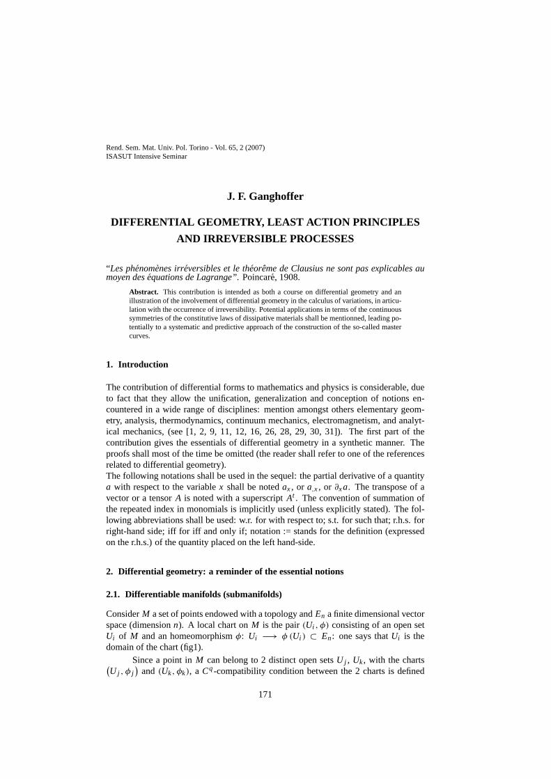
ConsiderM a set of points endowed with a topology andEn a finite dimensional vectorspace (dimensionn). A local chart onM is the pair(Ui , φ) consisting of an open setUi of M and an homeomorphismφ: Ui −→ φ (Ui ) ⊂ En: one says thatUi is thedomain of the chart (fig1).

Since a point inM can belong to 2 distinct open setsU j , Uk, with the charts(

U j , φ j)

and (Uk, φk), a Cq-compatibility condition between the 2 charts is defined

171

172 J. F. Ganghoffer

Figure 1: Chart of a manifold.

asU j ∩ Uk 6= ∅ ⇒ φk ◦ φ−1j

∣

∣

∣

U j ∩Ukis a diffeomorphism of classCq between the open

setsφ j(

U j ∩ Uk)

andφk(

U j ∩ Uk)

. Pointsp on M are conveniently labeled by localcoordinatesxi , which are the coordinates inRn of the pointφ(p). An atlas of classCq

on M is a set of charts(Ui , φi )i , s.t. the domains of the charts coverM ; all charts ofthe atlas areCq-compatible.

EXAMPLE 1. Consider the sphere of radius unity in 3D space, defined by

S2 =(

(x1, x2, x3) ∈ R3/

3∑

i=1

x2i = 1

)

the stereographic projection of the North polen onto the plane defined byx3 = 0 is abijection betweenS2 \ {n} and this plane. A similar projection of the South Pole canbe defined.

In the following, the base of the topology ofM is supposed countable, thus themanifold M is supposed separable. Submanifolds ofR

n+k can be defined from thenotions of submersion and immersion. ForU open inR

n, aC∞ mapψ : U → Rn+k

is an immersion if its differentialdψ(u) ∈ L(

TuRn → Tψ(u)Rn+k

)

is a one-to-onemap at everyu ∈ U . The linear algebra characterization of an immersion is that thedifferential dψ(u) induces a one to one linear map fromRn to R

n+k (equivalently,the differential mapdψ(u) has rankn). The dual notion of submersion is definedin the following manner: forV open inR

n+k, and f :→ Rk a smooth map,f is a

submersionif its differential D f (x) ∈ L(

TxRn+k → T f (x)R

k)

in an onto map, thuswhen the matrixD f (x) has rankk.

EXAMPLE 2. Consider the casen = 2 andk = 1; for h ∈ C∞ (R) a strictlypositive function, the map which rotates the curvex = h(z) around thez axis, namely

Differential geometry, least action principles 173

ψ(u, θ) = (h(u) cos(θ), h(u) sinθ,u) gives a parameterized surface of revolution. Thedifferential is

Dψ (u, θ) =

h′(u) cosθ −h(u) sinθh′(u) sinθ h(u) cosθ

1 0

,

the column of which being independent, thusψ is an immersion. As an example ofan submersion, let considerV =

{

(x1, x2, x3) x21 + x2

2 + x23 > 0

}

, and the functionf (x1, x2, x3) = x2

1 + x22 + x2

3. Its differential is D f (x1, x2, x3) = 2(x1, x2, x3),which is not zero onV , thus f is a submersion.Manifolds can be parametrized as curves and surfaces traditionally; considerM asa subset ofRn+k; an n-dimensional parametrization ofM is given by a one-to-oneimmersionψ : W → U ⊂ R

n+k, with U an open subset ofRn+k with U ∩ M 6= ∅,andψ(W) = U ∩ M . The image of a 1D parametrization is a parametrized curve, andthat of a 2D parametrization is a parametrized surface. For instance, the application

θ : (0,2π) → U = R2(1,0)

θ 7→ (cosθ, sinθ)

gives a 1D parametrization of the unit circle inR2.The implicit function theorem gives a convenientimplicit function parametrization,i.e. one having the special formψ (x1, . . . , xn, h1(x), . . . , hn(x)), with h an implicitfunction.For example, a 2D implicit function parametrization at the point(0,0,1) of the sphere

S2 in R3 is given byψ(x, y) =

(

x, y,√

1 − x2 − y2)

, with domain

W ={

(x, y) ∈ R2/x2 + y2 < 1

}

and rangeW × (0,+∞).

2.2. Transformations, Lie groups and Lie derivatives

Generally speaking, transformations map a set into itself,and a mathematical structurecam be characterized by those transformations that leaves it invariant (for instance,Euclidean geometry is invariant under orthogonal transformations, whereas special rel-ativity has a structure compatible with invariance w.r. to the Lorentz group). Veryoften, transformations establish as a group, and the prime tool there is the infinitesimaltransformation, which is described by a vector field (an infinitesimal generator of thegroup).To each point of the manifold can be attached an n-dimensional vector space, calledthe tangent space (local notion). At a pointp0 ∈ M , let define thegermof a differ-entiable functiong as the equivalence class of differentiable functions that coincide inan open neighborhood ofp0. Furthermore, atangent vector is an equivalence classof curves having the same tangency atp0; the curvesc : I ⊂ R → M are tangent


at a pointp0, if, in a given chart(Uφ), they give the same valued

dt(φ ◦ c)(0), with

p0 = c(0). Using further the composition of functions theorem gives the rate of varia-tion of the functiong along the curvec (i.e. the composite mapg ◦ φ−1 : R

n → R),

asd

dt(g ◦ c)(0) =

n∑

I =1

(

∂g

∂xi

)

x0

dxi

dt(0). Thereby, the notion of tangent vector re-

ceives a second definition: the tangent vector also is derivation acting on the set ofgerms of functions defined in an open neighborhood ofp0, i.e. a linear applicationXp0 : g 7→ Xp0(g) = d

dt (g ◦ c)(0). Thus, the vector fieldXp0 has the coordinatesdxi

dt(0) (in the local basis(xi )i ), and is given intrinsically byXp0 =

(

dxi

dt

)

x0

∂

∂xi. It

is easy to see that the value of the action ofXp0 on any function is the same for anyrepresentant in the class of curves having he same tangent atp0.

DEFINITION 1. The tangent space to M at the point p0 is the set of equivalenceclasses of tangent curves to M at p0; it is also the set of tangent vectors to M at p0. Itis noted Tp0 M, and its dimension is n. The notion of tangent space to a manifold allowsan intrinsic definition of the differential (independent from the local coordinates).

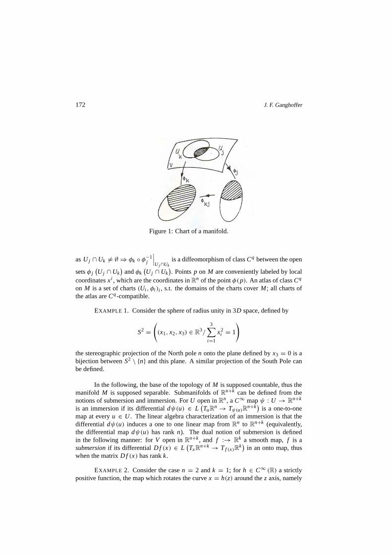
ForVn,Wm differentiable manifolds,f : Vn → Wm differentiable,X0 a tangentvector toVn at pointx0, with z0 = f (x0) ∈ W ∈ Wm, the differential of f at x0 is thelinear applicationd fx0 : Tx0Vn → Tz0Wm; X0 7→ d fx0 X0, s.t. ∀h, d fx0 X0( f ∗h), seefig 2. The applicationf ∗ therein is the reciprocal image

Figure 2: Differentiable functions and tangent mappings between manifolds.

The vectorZ0 := d fx0 X0 is tangent toWm at z0. In local coordinates, onesimply has

Z j = ∂ f j

∂xi(x0) Xi


and the matrix of elements

{

∂ f i

∂xi(x0)

}

i, jtherein is the Jacobean matrix. This notion

obviously reminds the transformation gradient in continuum mechanics.

DEFINITION 2 (Derivation). A derivation is a first-order differential operator,which is sensitive only to linear terms, thus a derivation X shall operate on productsof functions according to the rule X( f g) = f X(g)+ gX( f ). This defines the Leibnizrule for derivatives that warrants X being insensitive to quadratic and higher-orderterms (as shown earlier, vector fields act as derivations).

For two vector fieldsX,Y acting on functions, the double operationXY alsomaps functions to functions, but is not a derivation. As an example, any derivationat the point(0,0) acting on the functionf (x, y) = x2 + y2 must give zero (useLeibniz rule). But, composing∂x with itself gives∂x∂x f (x, y) = 2, thus∂x ◦ ∂x

is not a derivation (and the composition of derivations doesnot give a derivationin general). However, the operation ofLie bracketrestores the property of beinga derivation: it is defined by[XY − Y X], which in 3-vector notation would read[X,Y] = (X · ∇)Y − (Y · ∇) X. The Lie bracket receives an important geometricinterpretation, in connection toFrobenius Theorem: if at every point, the Lie bracketof tangent vectors to two families of curves are a linear combination of the two vec-tors, the curves then fit together to define a 2-surface. This can easily be generalized tohigher dimension.

DEFINITION 3. A Lie group G is a set that both has the structure of a groupand of a manifold. Thus, it is a differentiable manifold of class C∞, and the groupstructure is characterized by the following operations (product and inversion)

G × G → G; (x, y) 7→ xy; G → G; x 7→ x−1.

Every neighborhood ofe is then sent byL y to a neighborhood ofy by the lefttranslation; the differential applicationdLy : TeG → TyG allows the definition of leftinvariant vector fields:∀y ∈ G, dLy X(e) = X(y).

It can easily be shown that the left invariant vector fields onG have a vectorialstructure (same dimension asG), and that this vectorial space is isomorphic to thetangent spaceTeG. Furthermore, the bracket of two left invariant vector fields is itselfa left invariant vector field, namely one hasdLy [X,Y] (e) =

[

dLy X,dLyY]

(e) =[X,Y](y). The left invariant vector fields on the Lie groupG thus have the structure ofLie algebra.

DEFINITION 4. The Lie algebra of the Lie group G is the Lie algebra of theleft invariant vector fields. A Lie group action on a manifoldM is given by a mapµ : G × M → M; (a,q) 7→ µa(q), satisfyingµe(q) = q and the composition ruleµa ◦ µb = µab. Lie groups and Lie algebra are most of the case discussed in terms oftheir matrix representations.

EXAMPLE 3. The Lorentz group action inE D space-time can be represented


by the one-parameter family of matrices[

chψ shψ,shψ chψ,

]

which defines a one-dimensional group (identity element is given byψ = 0), withgroup manifoldR. The group action onR2 is defined by the application

(t, x) 7→ (t, chψ + x shψ, t shψ + x chψ)

The Lie algebra is endowed with the bracket operation (of vector fields); it sat-isfies the properties of linearity, anticommutativity([X,Y] = −[Y, X]), and the Jacobiidentity ([X, [Y, Z]] + [Y, [Z, X]] + [Z, [X,Y]] = 0).Once the action of a transformation on points is defined, the action on tangent vec-tors (or more generally on elements of the tangent bundle), on tensors and differentialforms (on elements of the cotangent bundle) are determined.The change operated onthose objects is called theLie derivative. Recall that any differentiable vector fieldXon a manifoldM generates a 1-parameter local group of diffeomorphismsφt relatingneighborhoods ofM , viz φt : M → M x 7→ φt x, that satisfies the differential equation

dφt

dt= X (φt x)

with the initial conditionφ0(x) = x. The orbit of the group passing through pointx0 = φ(x0) is the integral curveR → M; 7→ x(t) = φt x0 tangent to the vectorsX (φt x0) of the field at each pointφt x0. Since the manifolds (contrary to the Euclideanspaces) do not allow an easy comparison of vector fields attached at different points(thus leaving in different vectorial spaces), a novel derivative needs to be introduced.Considerg a differentiable function onM ; the tangent vector to the groupφt at the

point x0 is X0 =(

d

dtx(t)

)

t=0=(

d

dtφt x0

)

t=0. The derivative of (the germ of)

g in the direction ofX at the pointx0 is the realX0 g =(

d

dt( f ◦ φt ) (x0)

)

t=0=

X I(

∂

∂xig

)

x I0

(

dxi

dt

)

0.

• The Lie derivative of the functiong in the direction ofX at pointx0, is defined as

the directional derivativeLx0g = X0g = limt→0

g (φt x0)− g (x0)

t. The operation

achieved therein means a pull-back along the orbit to the point x0, comparing thevalueg (φt x0) to the valueg (x0) at the same point. In a set of local coordinates,one writes

Lxg = X I ∂i g

• The Lie derivative of the vector fieldY in the direction of the vector fieldX at

point x0 is L XY = limt→0

1

t

(

dφ−1t Yφt x0 − Yx0

)

=(

d

dtdφt−1Y

)

t = 0. It can be


proven that the Lie derivative coincides with the Lie bracket L XY = [X,Y]. Ina set of local coordinates, one writes

L XY =(

X j ∂ j YI − Y j ∂ j Xi

)

∂ i .

• The Lie derivative of a

(

q0

)

tensor field is similarly defined as

L XT := limt→0

1

t

(

dφ−1t Tφt x0 − Yx0

)

• Notingφ∗t Tφt x0 the pull-back at pointx0 of the tensorTφt x0, the Lie derivative of

a

(

0p

)

tensor field is elaborated as

L XT := limt→0

1

t

(

φ∗t Tφt x0 − Yx0

)

=(

d

dtφ∗

t T

)

t=0

• Similarly, for completely antisymmetrical tensors of the previous type, i.e. fordifferential formsω, the Lie derivative is defined as

(L Xω)x0= lim

t→0

1

t

(

φ∗t ωφt x0−ωx0

)

=(

d

dtφ∗

t ω

)

t=0

In a set of local coordinates, one writes for the Lie derivative of a 1-form(L Xω)I = X j ∂ jωi + ω j ∂i X j .

Properties

Only the essential properties of the differential operations so far introduced are listedin the sequel. A vector fieldν s.t. Lwν = 0 is said to beLie-transported or draggedalong the vector fieldw. Since the Lie derivative is a local approximation, it shallsatisfy Leibniz rule, thus

Lw (a ⊗ b) = Lwa ⊗ b + a ⊗ Lwb.

Using the same rule gives the Lie derivative of a 1-formα: differentiating the functionf = α.ν renders(Lwα) .ν = d (α.ν)w − α [w, ν] , thus in terms of a set of coordi-natesLwα =

(

αµ, θwν + αθwν, ν)

dxν . Lie derivatives inform about symmetries ofgeometrical objects; so for instance, the infinitesimal symmetries of the 1-form field

dx are given by those vector fieldsw = X∂

∂x+ Y

∂

∂y+ Z

∂

∂z, that satisfiesLwdx = 0,

thusX has to be constant.


2.3. Calculus on differential forms

Differential forms find their origin in 1889 in the work of Elie Cartan(1869− 1951),and in the third volume ofLes Methodes Nouvelles de la Mecanique Celesteby HenriPoincare (1854− 1912). The program of writing the laws of physics in an invariantform (using differential forms), was started by g. Ricci-Curbastro(1853− 1925) andhis student T. Levi-Civita(1873− 1941); it provided the useful framework for A.Einstein(1879− 1955) to develop the theory of relativity.ConsiderM an n-dimensional manifold and(x1, x2, . . . , xn) a coordinate system onthis manifold.

DEFINITION 5. A p-form or exterior form of degree p on M is alternated orcompletely antisymmetrical if it is the antisymmetrical part of a multilinear applica-tion from M toR. Thus, for tx a p-linear form (at point x of M), the operation ofantisymmetrization renders

Ap tx (V1, . . . ,Vn) = 1

p!∑

σ

ǫσ tx(

Vσ(1), . . . ,Vσ(p))

,

with σ a permutation having the signatureǫσ .

A p-form can be built from the tensorial product of n one-forms on M , accord-ing to the rule: the tensorial product ofp 1-forms is thep-form, the components ofwhich are identified with the components of the tensorial product if the p associatedvectors.

EXAMPLE 4. Considerα(x1 x2) = 3x2− x1 andβ(x1 x2) = 2x2 + x1; one thenhas

α ⊗ β = (x1, x2)

[(

−13

)

⊗(

12

)](

x1x2

)

=

= (x1 x2)

(

−1 −23 6

)(

x1x2

)

= −x21 + x1x2 + 6x2

2

DEFINITION 6. The exterior product (notation∧) of p 1-forms Aik , is the p-form obtained by the anti symmetrization of the tensorial product, viz

Ai 1 ∧ Ai 2 . . . ∧ Ai p = δi1...i pI1...I p

AI1 ⊗ . . .⊗ AI p

(summation of the indices Ik), with

δi1...i pI1...I p

=

0 if the ik are not a permutation of the Ik

1 if the ik are an even permutation of the Ik

−1 if the ik are an odd permutation of the Ik

EXAMPLE 5. One has inR4 the equality

x3 ∧ x1 = x3 ⊗ x1 − x1 ⊗ x3 = −x1 ∧ x3


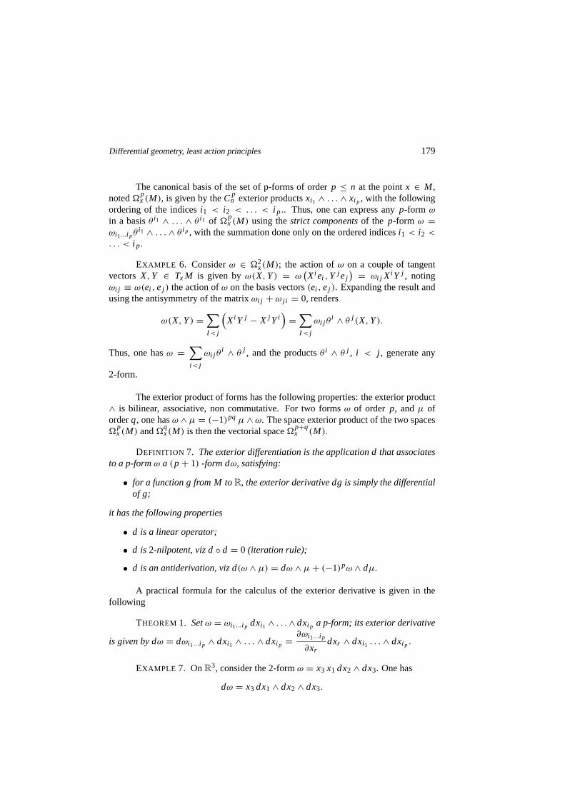
The canonical basis of the set of p-forms of orderp ≤ n at the pointx ∈ M ,noted�p

x (M), is given by theCpn exterior productsxi1 ∧ . . . ∧ xi p , with the following

ordering of the indicesi1 < i2 < . . . < i p.. Thus, one can express anyp-form ω

in a basisθ i1 ∧ . . . ∧ θ i1 of �px (M) using thestrict componentsof the p-form ω =

ωi1...i pθi1 ∧ . . . ∧ θ i p , with the summation done only on the ordered indicesi1 < i2 <

. . . < i p.

EXAMPLE 6. Considerω ∈ �2x(M); the action ofω on a couple of tangent

vectors X,Y ∈ Tx M is given byω(X,Y) = ω(

Xi ei ,Y j ej)

= ωi j Xi Y j , notingωi j ≡ ω(ei ,ej ) the action ofω on the basis vectors(ei ,ej ). Expanding the result andusing the antisymmetry of the matrixωi j + ω j i = 0, renders

ω(X,Y) =∑

I< j

(

Xi Y j − X j Yi)

=∑

I< j

ωi j θi ∧ θ j (X,Y).

Thus, one hasω =∑

i< j

ωi j θi ∧ θ j , and the productsθ i ∧ θ j , i < j , generate any

2-form.

The exterior product of forms has the following properties:the exterior product∧ is bilinear, associative, non commutative. For two formsω of order p, andµ oforderq, one hasω ∧ µ = (−1)pqµ∧ ω. The space exterior product of the two spaces�

px (M) and�q

x(M) is then the vectorial space�p+qx (M).

DEFINITION 7. The exterior differentiation is the application d that associatesto a p-formω a (p + 1) -form dω, satisfying:

• for a function g from M toR, the exterior derivative dg is simply the differentialof g;

it has the following properties

• d is a linear operator;

• d is2-nilpotent, viz d◦ d = 0 (iteration rule);

• d is an antiderivation, viz d(ω ∧ µ) = dω ∧ µ+ (−1)pω ∧ dµ.

A practical formula for the calculus of the exterior derivative is given in thefollowing

THEOREM1. Setω = ωi1...i p dxi1 ∧ . . .∧ dxi p a p-form; its exterior derivative

is given by dω = dωi1...i p ∧ dxi1 ∧ . . . ∧ dxi p =∂ωi1...i p

∂xrdxr ∧ dxi1 . . . ∧ dxi p .

EXAMPLE 7. OnR3, consider the 2-formω = x3 x1 dx2 ∧ dx3. One has

dω = x3 dx1 ∧ dx2 ∧ dx3.


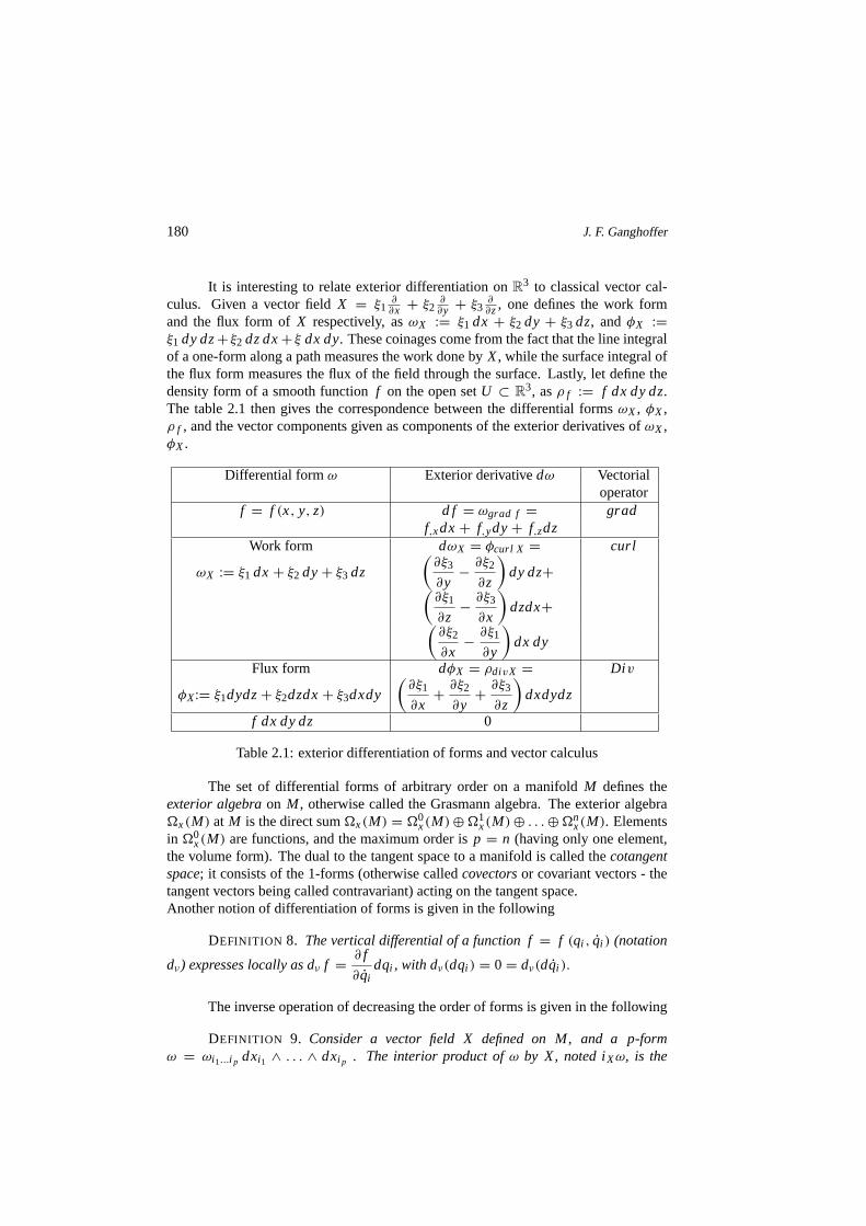
It is interesting to relate exterior differentiation onR3 to classical vector cal-

culus. Given a vector fieldX = ξ1∂∂x + ξ2

∂∂y + ξ3

∂∂z, one defines the work form

and the flux form ofX respectively, asωX := ξ1 dx + ξ2 dy + ξ3 dz, andφX :=ξ1 dy dz+ ξ2 dz dx+ ξ dx dy. These coinages come from the fact that the line integralof a one-form along a path measures the work done byX, while the surface integral ofthe flux form measures the flux of the field through the surface.Lastly, let define thedensity form of a smooth functionf on the open setU ⊂ R

3, asρ f := f dx dy dz.The table 2.1 then gives the correspondence between the differential formsωX , φX ,ρ f , and the vector components given as components of the exterior derivatives ofωX ,φX .

Differential formω Exterior derivativedω Vectorialoperator

f = f (x, y, z) d f = ωgrad f = gradf,xdx + f,ydy + f,zdz

Work form dωX = φcurl X = curl

ωX := ξ1 dx + ξ2 dy + ξ3 dz

(

∂ξ3

∂y− ∂ξ2

∂z

)

dy dz+(

∂ξ1

∂z− ∂ξ3

∂x

)

dzdx+(

∂ξ2

∂x− ∂ξ1

∂y

)

dx dy

Flux form dφX = ρdivX = Di v

φX:= ξ1dydz+ ξ2dzdx+ ξ3dxdy

(

∂ξ1

∂x+ ∂ξ2

∂y+ ∂ξ3

∂z

)

dxdydz

f dx dy dz 0

Table 2.1: exterior differentiation of forms and vector calculus

The set of differential forms of arbitrary order on a manifold M defines theexterior algebraon M , otherwise called the Grasmann algebra. The exterior algebra�x(M) at M is the direct sum�x(M) = �0

x(M)⊕�1x(M)⊕ . . .⊕�n

x(M). Elementsin �0

x(M) are functions, and the maximum order isp = n (having only one element,the volume form). The dual to the tangent space to a manifold is called thecotangentspace; it consists of the 1-forms (otherwise calledcovectorsor covariant vectors - thetangent vectors being called contravariant) acting on the tangent space.Another notion of differentiation of forms is given in the following

DEFINITION 8. The vertical differential of a function f= f (qi , qi ) (notation

dν) expresses locally as dν f = ∂ f

∂qidqi , with dν(dqi ) = 0 = dν(dqi ).

The inverse operation of decreasing the order of forms is given in the following

DEFINITION 9. Consider a vector field X defined on M, and a p-formω = ωi1...i p dxi1 ∧ . . . ∧ dxi p . The interior product ofω by X, noted iXω, is the


(p − 1)-form iXω := 1

(p − 1)! ωki2...i p Xk dxi2 ∧ . . . ∧ dxi p .

EXAMPLE 8. consider onR2 the 1-formω = x2 dx1 and the vector field

X = x2∂

∂x1+ ∂

∂x2;

the direct application of previous definition givesi X ω = ωk Xk = x22.

Properties

The following identity is often referred to asCartan identity

Lνω = iνdω + d (iνω) .

One further list some basic properties (without proof):

iν(ω ∧ v) = (iνω) ∧ v + (−1)pω ∧ (Iνv)

Lνdω = dLνω; Lν (iuω) = i [ν,µ]ω + iuLvω;L f να = f Lνα + d f ∧ (iνα)

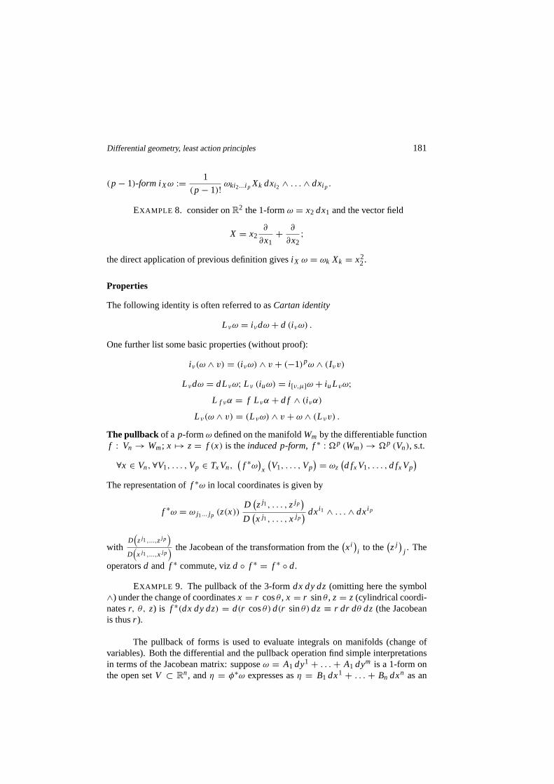
Lν(ω ∧ v) = (Lνω) ∧ v + ω ∧ (Lνv) .The pullback of a p-formω defined on the manifoldWm by the differentiable functionf : Vn → Wm; x 7→ z = f (x) is theinduced p-form, f ∗ : �p (Wm) → �p (Vn), s.t.

∀x ∈ Vn,∀V1, . . . ,Vp ∈ TxVn,(

f ∗ω)

x

(

V1, . . . ,Vp)

= ωz(

d fxV1, . . . ,d fxVp)

The representation off ∗ω in local coordinates is given by

f ∗ω = ω j1... j p (z(x))D(

z j1, . . . , z j p)

D(

x j1, . . . , x j p) dxi1 ∧ . . . ∧ dxi p

withD(

z j1,...,z j p)

D(

x j1,...,x j p) the Jacobean of the transformation from the

(

xi)

i to the(

z j)

j . The

operatorsd and f ∗ commute, vizd ◦ f ∗ = f ∗ ◦ d.

EXAMPLE 9. The pullback of the 3-formdx dy dz(omitting here the symbol∧) under the change of coordinatesx = r cosθ , x = r sinθ , z = z (cylindrical coordi-natesr, θ, z) is f ∗(dx dy dz) = d(r cosθ)d(r sinθ)dz ≡ r dr dθ dz (the Jacobeanis thusr ).

The pullback of forms is used to evaluate integrals on manifolds (change ofvariables). Both the differential and the pullback operation find simple interpretationsin terms of the Jacobean matrix: supposeω = A1 dy1 + . . . + A1 dym is a 1-form onthe open setV ⊂ R

n, andη = φ∗ω expresses asη = B1 dx1 + . . . + Bn dxn as an


1-form on the open setU ⊂ Rn, with φ : U → V a diffeomorphism. Representingω

andη as the row vectorsEω = [A1, . . . , Am] andEη = [B1, . . . , Bn] then gives

[B1, . . . , Bn] = [ A1, . . . , Am]

D1φ1 . . . Dnφ

1

. . . . . . . . .

D1φm . . . Dnφ

m

Thus, the pullback of a 1-form corresponds to matrix post-multiplication. As an appli-cation, whenp = n = m, one recovers the change of variable formula used in the the-ory of integration, vizω = A

(

dy1 ∧ . . . ∧ dyn)

⇒ φ∗ω = |Dφ| A(

dx1 ∧ . . . ∧ dxn)

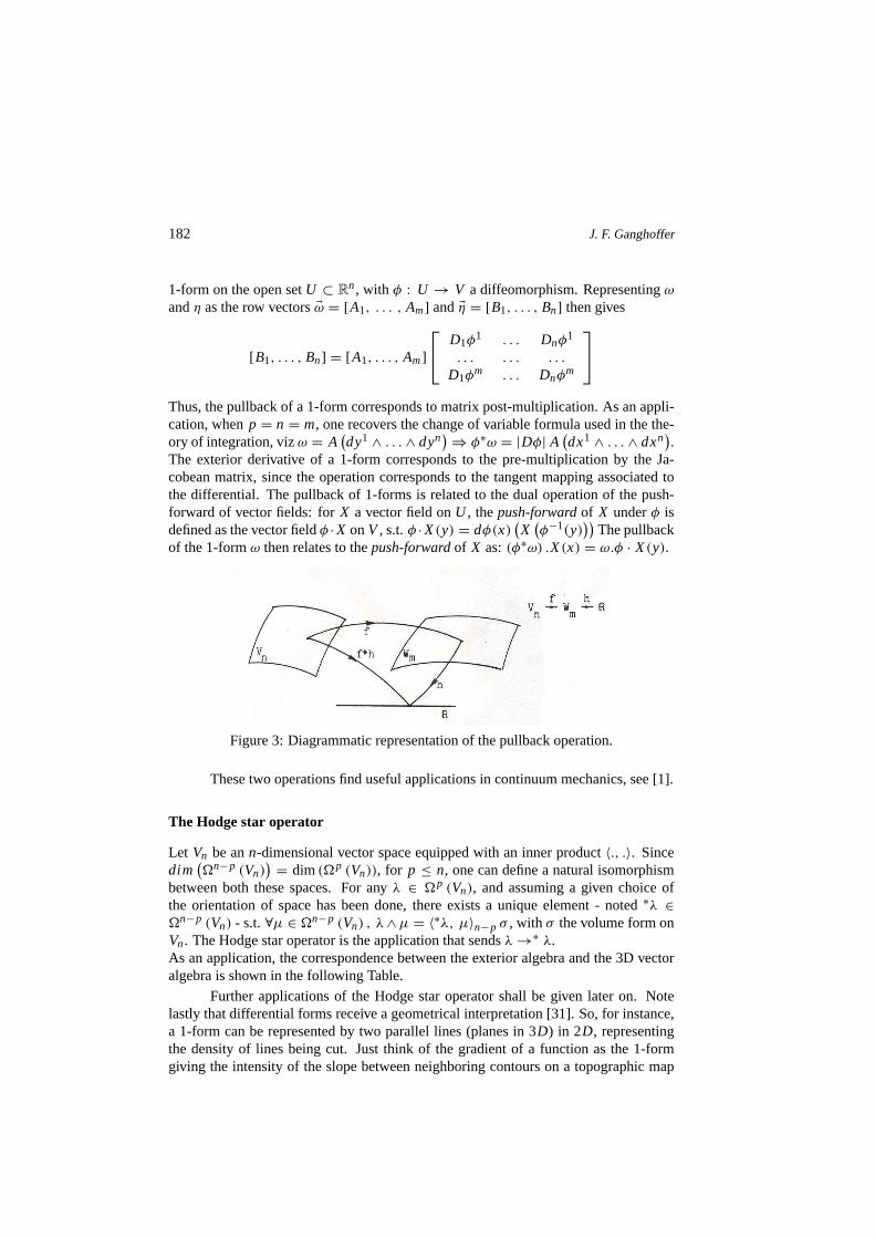
.The exterior derivative of a 1-form corresponds to the pre-multiplication by the Ja-cobean matrix, since the operation corresponds to the tangent mapping associated tothe differential. The pullback of 1-forms is related to the dual operation of the push-forward of vector fields: forX a vector field onU , thepush-forwardof X underφ isdefined as the vector fieldφ · X onV , s.t.φ · X(y) = dφ(x)

(

X(

φ−1(y)))

The pullbackof the 1-formω then relates to thepush-forwardof X as:(φ∗ω) .X(x) = ω.φ · X(y).

Figure 3: Diagrammatic representation of the pullback operation.

These two operations find useful applications in continuum mechanics, see [1].

The Hodge star operator

Let Vn be ann-dimensional vector space equipped with an inner product〈., .〉. Sincedim

(

�n−p (Vn))

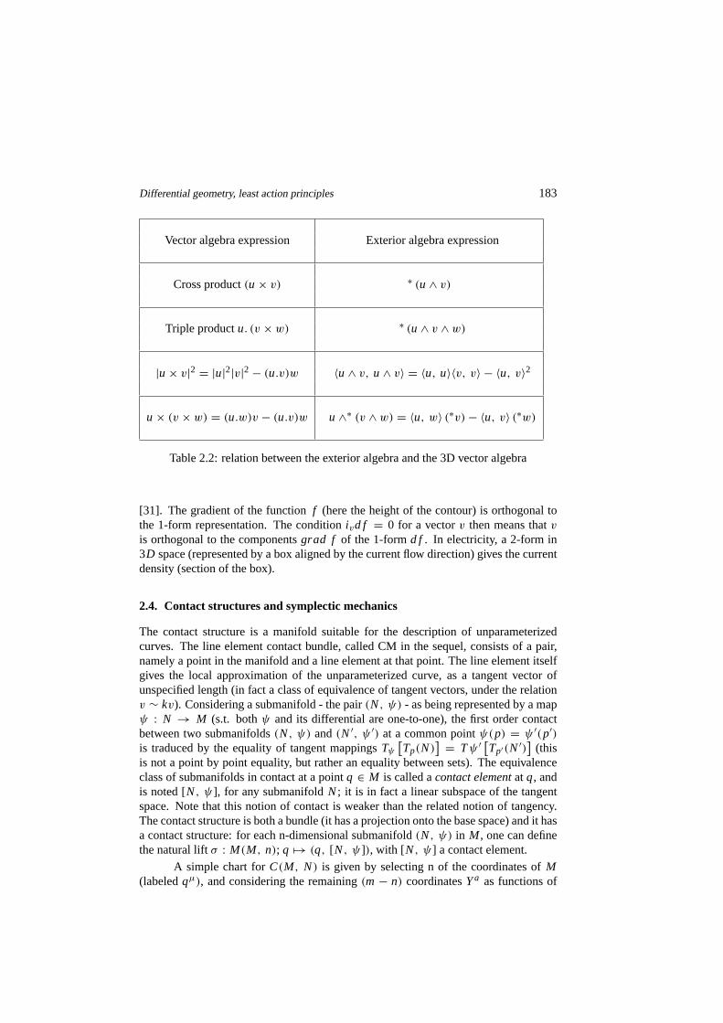
= dim(�p (Vn)), for p ≤ n, one can define a natural isomorphismbetween both these spaces. For anyλ ∈ �p (Vn), and assuming a given choice ofthe orientation of space has been done, there exists a uniqueelement - noted∗λ ∈�n−p (Vn) - s.t.∀µ ∈ �n−p (Vn) , λ∧µ = 〈∗λ, µ〉n−p σ , with σ the volume form onVn. The Hodge star operator is the application that sendsλ →∗ λ.As an application, the correspondence between the exterioralgebra and the 3D vectoralgebra is shown in the following Table.

Further applications of the Hodge star operator shall be given later on. Notelastly that differential forms receive a geometrical interpretation [31]. So, for instance,a 1-form can be represented by two parallel lines (planes in 3D) in 2D, representingthe density of lines being cut. Just think of the gradient of afunction as the 1-formgiving the intensity of the slope between neighboring contours on a topographic map


Vector algebra expression Exterior algebra expression

Cross product(u × v) ∗ (u ∧ v)

Triple productu. (v × w) ∗ (u ∧ v ∧ w)

|u × v|2 = |u|2|v|2 − (u.v)w 〈u ∧ v, u ∧ v〉 = 〈u, u〉〈v, v〉 − 〈u, v〉2

u × (v × w) = (u.w)v − (u.v)w u ∧∗ (v ∧ w) = 〈u, w〉 (∗v)− 〈u, v〉 (∗w)

Table 2.2: relation between the exterior algebra and the 3D vector algebra

[31]. The gradient of the functionf (here the height of the contour) is orthogonal tothe 1-form representation. The conditionivd f = 0 for a vectorv then means thatvis orthogonal to the componentsgrad f of the 1-formd f . In electricity, a 2-form in3D space (represented by a box aligned by the current flow direction) gives the currentdensity (section of the box).

2.4. Contact structures and symplectic mechanics

The contact structure is a manifold suitable for the description of unparameterizedcurves. The line element contact bundle, called CM in the sequel, consists of a pair,namely a point in the manifold and a line element at that point. The line element itselfgives the local approximation of the unparameterized curve, as a tangent vector ofunspecified length (in fact a class of equivalence of tangentvectors, under the relationv ∼ kv). Considering a submanifold - the pair(N, ψ) - as being represented by a mapψ : N → M (s.t. bothψ and its differential are one-to-one), the first order contactbetween two submanifolds(N, ψ) and(N′, ψ ′) at a common pointψ(p) = ψ ′(p′)is traduced by the equality of tangent mappingsTψ

[

Tp(N)]

= Tψ ′ [Tp′(N′)]

(thisis not a point by point equality, but rather an equality between sets). The equivalenceclass of submanifolds in contact at a pointq ∈ M is called acontact elementat q, andis noted[N, ψ ], for any submanifoldN; it is in fact a linear subspace of the tangentspace. Note that this notion of contact is weaker than the related notion of tangency.The contact structure is both a bundle (it has a projection onto the base space) and it hasa contact structure: for each n-dimensional submanifold(N, ψ) in M , one can definethe natural liftσ : M(M, n); q 7→ (q, [N, ψ ]), with [N, ψ ] a contact element.

A simple chart forC(M, N) is given by selecting n of the coordinates ofM(labeledqµ), and considering the remaining(m − n) coordinatesYa as functions of


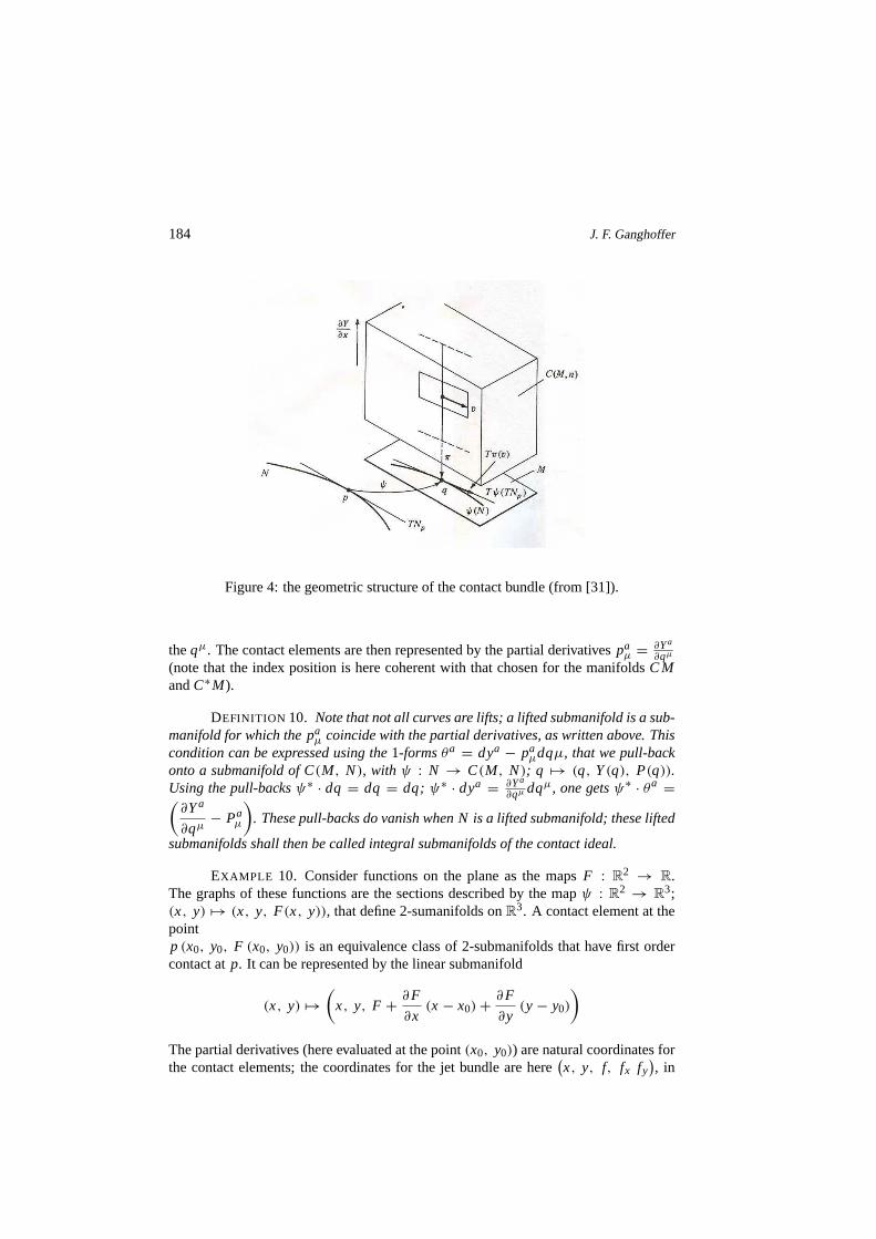
Figure 4: the geometric structure of the contact bundle (from [31]).

theqµ. The contact elements are then represented by the partial derivatives paµ = ∂Ya

∂qµ

(note that the index position is here coherent with that chosen for the manifoldsC MandC∗M).

DEFINITION 10. Note that not all curves are lifts; a lifted submanifold is a sub-manifold for which the paµ coincide with the partial derivatives, as written above. Thiscondition can be expressed using the1-formsθa = dya − pa

µdqµ, that we pull-backonto a submanifold of C(M, N), with ψ : N → C(M, N); q 7→ (q, Y(q), P(q)).Using the pull-backsψ∗ · dq = dq = dq; ψ∗ · dya = ∂Ya

∂qµ dqµ, one getsψ∗ · θa =(

∂Ya

∂qµ− Pa

µ

)

. These pull-backs do vanish when N is a lifted submanifold; these lifted

submanifolds shall then be called integral submanifolds ofthe contact ideal.

EXAMPLE 10. Consider functions on the plane as the mapsF : R2 → R.

The graphs of these functions are the sections described by the mapψ : R2 → R

3;(x, y) 7→ (x, y, F(x, y)), that define 2-sumanifolds onR3. A contact element at thepointp (x0, y0, F (x0, y0)) is an equivalence class of 2-submanifolds that have first ordercontact atp. It can be represented by the linear submanifold

(x, y) 7→(

x, y, F + ∂F

∂x(x − x0)+ ∂F

∂y(y − y0)

)

The partial derivatives (here evaluated at the point(x0, y0)) are natural coordinates forthe contact elements; the coordinates for the jet bundle arehere

(

x, y, f, fx fy)

, in


which fx, fy are coordinates of the contact element (and not partial derivatives). Thepull-back of the contact 1-formθ := d f − fxdx − fydy onto a submanifold definedby the applicationψ : (x, y) 7→

(

x, y, F, Fx Fy)

givesψ∗ · θ = ∂F∂x dx + ∂F

∂y dy −Fxdx − Fydy, which vanishes whenFx = ∂F

∂x ; Fy = ∂F∂y . The geometric approach to

the calculus of variations presents some interest because of its originality, compared tothe standard approach. The standard formulation of the classical mechanics of uncon-strained conservative systems states the existence of a Lagrangian functionL, depend-ing upon the state variables and possibly upon time, such that the action integral

∫

L dtis extremized. On the contact bundle of the configuration space, having the naturalcoordinates(t, q, q), the integrand

∫

L dt is a one-form. The possible motions of thesystem are then described by the curves in the contact bundleon which the contact 1-formsα := dq− q dt pull back to zero. The variation of the action integral around the

extrema is further performed, using the vector fieldv = Q(t)∂

∂q+ Q(t)

∂

∂q, restricting

to isochronal variations. Restricting further to variations with fixed end conditions, thevariation is given by

∫

Ŵ

Lv (L dt) =∫

Ŵ

iv (dL dt) =∫

Ŵ

[

Q∂L

∂qdt + Q

∂L

∂qdt

]

In order now for the variations to satisfy the previous constraint condition, the vectorfield v has to move the initial path into a path that is parallel to theα; instead ofpushing the path forward, one can equivalently pull back the1-formsα, asα(ǫ) =α+ǫLvα. The condition that the 1-formα(ǫ) pulls backs to zero on the integral curve,viz i γ α(ǫ) = 0, rendersi γ Lvα = 0, thusi γ

(

d Q − Q dt)

= 0. Since integration overthe optimal path is equivalent to contracting the integrandwith γ , using the previousequation allows to replaceQ dt by d Q, thus

Lv

∫

Ŵ

L dt =∫

Ŵ

[

Q∂L

∂qdt + ∂L

∂qd Q

]

Integrating the second term by part and omitting the perfectdifferential (since we con-sider fixed ends) renders

Lv

∫

Ŵ

L dt =∫

Ŵ

Q

[

∂L

∂qdt + d

(

∂L

∂q

)]

The arbitrariness in the choice of the functionsQ(t) then leads to the condition

i γ

{

∂L

∂qdt + d

(

∂L

∂q

)}

= 0

for γ to be tangent to the path.This condition together with the constraint

I γ (dq − qdt) = 0

gives 2n relations for the 2n components of the line element.SinceL dt is not a general 1-form (its exterior derivativedL dt being in the differential


ideal generated byL dt) , anddα also is in the ideal generated byL dt, a more generalviewpoint is needed. Let then enlarge the previous considerations, starting first from theextemum condition of unconstrained integrals of the formI =

∫

γω, with the smooth

enough 1-formω defined on a manifoldM , andŴ a curve inM (between two pointsAandB) s.t. the integralI does not vary at the first order asŴ is deformed. Consideringa curve parameterized bys, the tangent vector to the curveγ expresses as the push

forward of the basis vector∂

∂s, viz γ = Ŵ∗.

(

∂

∂s

)

. Let then continuously deform the

curveŴ by a vector fieldv; the previous condition that the integralI does not changeunder this deformation expresses as

∫

Ŵ

Lvω

Using the properties of the Lie derivatives further renders∫

Ŵ

iv dω +∫

Ŵ

iv ω = 0

Sincev vanishes at the end points (A andB being fixed), the boundary term vanishes.From the definition of a line integral, we further have

∫

Ŵ

iv dω =∫ b

aŴ∗.

(

iv(

i γ dω))

ds = 0,∀v,

thus the local conditioniv(

i γ dω)

= 0, ∀v, that further givesi γ dω = 0, which is anordinary differential equation forŴ.Using the local coordinatesxµ = xµ(s) along the curve, one can further elaborateprevious condition: the integralI =

∫

ωµ dxµdsrenders the Euler-Lagrange equations

ωµ,v xµ − d

dsωv = 0 thus giving the Schwarz condition

(

ωµ,v − ωv,µ)

xµ = 0. A first

insight into Noether’s theorem can here be given: suppose aninfinitesimal symmetry

exists, having the vector fieldk, such thatLkω = 0. This clearly gives∫

Ŵ

Lkω = 0;

along any piece of a curve that satisfies the Euler-Lagrange equations, the conditioni γ dω = 0 gives

∫

Ŵ

Lkω =∫

Ŵ

d (ikω)+∫

Ŵ

ikdω =∫

Ŵ

ikω = 0

which means that the quantityikω is constant along the solution curves. This is an il-lustration of Noether’s theorem, articulating infinitesimal symmetries and conservationlaws.The case of constrained variations is next treated, wherebythe constraint is expressedby the vanishing of some functionφ : M → R, in the case of holonomic variations:we require that the variation of the integralI =

∫

Ŵω vanishes, vizLv

∫

Ŵω = 0, for all

deformations of the curve that satisfy the constraintLvφ = ivdφ = 0. Summarizing,the variation of the integral must vanish at any point, viziv

(

i γ dω)

= 0, ∀v, for all v


satisfying the conditionivdφ = 0. This implies the existence of a multiplier functionλ = λ(s), s.t. the following condition holds along the curve:i γ dω = λdφ, whereφ = 0.This condition forms a set of determining equations for the curve and the Lagrangemultiplier λ. In the case of anholonomic variations, the constraints canbe expressedin the form i γ α = 0, for a set of prescribed 1-formsα. The extension of the vectorfield γ off the curve is done using the conditionLv γ = 0, thus the constraint conditioni γ Lvα = Lv

(

i γ α)

= 0.The optimal pathŴ is again determined by the conditioni γ d (ω + λα) = 0, along withi γ α = 0. To be complete, one can evidence a Lagrange multiplierλ s.t. an uncon-strained minimum exists for the problem having the one-formω+λα, see e.g [31]. Forthat purpose, a vector fieldw is selected s.t. the deformation of the curve can be writtenin the formv = vc+ξw, wherevc satisfies the constraint, andξ is a scalar function that

restores the degree of freedom lost in the constraint: it is foundξ = i γ Lvǫ

i γ (iwdα), under

the conditioniwdα 6= 0 (with dα 6= 0, otherwise the constraint would be integrable).Using next Cartan identity and neglecting the exact differentials gives the multiplier

λ = − i γ (iwdω)

i γ (iwdα).

EXAMPLE 11. The dynamic equations of motion of a conservative systemde-scribed by a LagrangianL (q, q, t) is given as the stationary conditions of the func-tional

∫

ŴL (q, q, t) dt, under the constraintsi γ (qdt − dq) = 0. Application of pre-

vious general methodology renders the multiplierλ = −∂L

∂q, and the equivalent un-

constrained problem is∫

Ŵ

[

Ldt − ∂L

∂q(qdt − dq)

]

, the Euler-Lagrange equations of

which being

i γ{

dLdt − d(

∂L∂q

)

(qdt − dq)− ∂L∂q

}

= i γ{

∂L∂q dq dt− d

(

∂L∂q

)

(qdt − dq)}

= 0.

It holds true that

i γ dq dt= i γ (dq − qdt) dt=− (dq − qdt)dt=− (dq − qdt)(

i γ dt)

the previous equation then gives

i γ{

dLdt−d(

∂L∂q

)

(qdt − dq)− ∂L∂q dqdt

}

= i γ{

∂L∂q dqdt−d

(

∂L∂q

)

(qdt−dq)}

=0

i γ

{

∂L

∂qdt −

(

∂L

∂q

)}

(qdt − dq) = 0

Consequently, the extremals are the integral curves of the 1-forms∂L

∂qdt − d

(

∂L

∂q

)

anddq − qdt.


The invariance of the constrained problem under infinitesimal symmetries againleads to the evidence of a conservation law: let indeed the vector k be an infinitesimalsymmetry of both the variational principle and of the constraint, viz Lvω = 0 andLvα = 0. Thus, the Lie derivative of the one-formα has to be in the ideal generatedby α (sincei γ α = 0). Incorporating the multiplier into the Lie differentiation thengives the conditionLk (ω + λǫ) ⊂ I [α], which traduces into a differential formatas∫

Ŵ{d (ω + λα)+ ikd (ω + λα)} = 0. The second term is identified as the Euler-

Lagrange equation (it vanishes), thus one obtains the conservation lawikd (ω + λα) =constant, along the extremals.

3. Lagrangian formalism and irreversibility

3.1. Differential structure of thermodynamics

A few words related to the geometrical setting of thermodynamics are first in order.Thermodynamic systems are described in the contact bundle sustained by the followingcoordinates:

• The total energy and entropy;

• the extensive variables (such as the volume, the number of particle, or the electriccharge), that are the measurable degrees of freedom;

• the intensive associated variables, which are forces or potentials that describe theenergy transfer between the various extensive variables.

EXAMPLE 12. An ideal gas is described in a 2D state space, with coordinatesentropy and volume. An open gaseous system would require theadditional coordinateof the amount of gas present in the system.

A thermodynamic system shall then be described by a linear structure, a contactstructure and a convexity structure: thelinear structureis a model for the physicalidea of short-range interactions and existence of homogeneous systems with a scalingsymmetry. Thecontact structureis associated with the energy conservation (first lawof thermodynamics), while theconvexity structureaccounts for the Second Law andthe entropy increase due to mixing. As a starting point, thefundamental equationconsists of the expression of the stored internal energy of the system for all possiblestates, versus the set of state variables. For instance, thefundamental equation of anaggregate ofN molecules of an ideal gas is

U (S V) = N5/3V−2/3 exp(2S/3N K) ,

with k the Boltzmann’s constant. Linear structures rely on the assumption that the sys-tem size is much larger than the range of its interactions, thus the internal energy isproportional to the size of any subsystem (the shape of the subsystem does not matter):


by Euler’s theorem (traducing here the homogeneity of degree one), this scaling sym-

metry givesU = S∂U

∂S+ V

∂U

∂V. Contrary to the status of the extensive variables, the

intensive variables do not change versus size (homogeneityof degree zero). The graphof the fundamental equation is an n-surface in an(n−1)-space, with the potentials (par-tial derivatives of the internal energy w.r. to the extensive variables) the components ofthe contact elements to that surface. The contact bundle consists of the(2n + 1)-spacewith coordinates the extensive variables, their associated intensive variables, and theinternal energy. The contact ideal is generated by the 1-form

α = dU +∑

(forces)d (extensive variables) .

EXAMPLE 13. The previously introduced ideal gas is modeled in the 5-dimen-sional contact bundle with coordinates(U, T, S, P, V), and a contact ideal generatedby the 1-formα = dU − T dS+ Pdv, with P = −∂ − VU; T = ∂SU . The previoushomogeneity condition becomesU = T S− PV, which is theGibbs-Duhem relation.In addition to the fundamental equation, the equation of state expressing the intensivevariables has to be specified. As an example, consider the ideal gas, which obeys therelation PV = NkT, together with the internal energy expressionU = 3/2NkT. Inthe contact manifold, the system is described by the following map

ψ : (S, V) 7→ (U, T, S, P, V) = (U (S, V) , T (S, V) , S, P (S, V) , V)

which expresses as

ψ : (S, V) 7→ (U, T, S, P, V) = (3/2NkT, T (S, V) , S, NkT/V, V) .

The functionsU , Y, P shall satisfy the two previous conditions, as well asψ∗.θ = 0,with the 1-formθ = dU −UV dV − up d P = dU − T dS+ PdV. Accounting for thepullbacks

ψ∗.dU = (3/2) Nk

(

∂T

∂SdS+ ∂T

∂VdV

)

; ψ∗.dS= dS; ψ∗.dV = dV

one obtains

ψ∗.θ = (3/2) Nk

(

∂T

∂SdS+ ∂T

∂VdV

)

− T dS+(

NkT

V

)

dV ≡ 0

The independence of the differential elements(dV, dT) then implies

1

T

∂T

∂S= 2/3Nk; 1

T

∂T

∂V= −2/3V

The integration of these two equations givesT = AV−2/3exp(2S/3Nk), thus we re-cover the fundamental equationU (U, V) = N5/3V−2/3exp(2S/3Nk). Note that thefactor N5/3 therein ensures the satisfaction of the homogeneity condition of U (a sys-tem of twice the volume, with twice the number of molecules has twice the energy).


Having so far developed what could be called a differential thermodynamics [31], theuse of Frobenius theorem closes the characterization of thestructure of thermodynam-ics: consider for instance the energy 2-surface as the mapR

2 → R3; (S, V) 7→

(U, S, V), with the intensities given byT = ∂SU and−P = ∂VU . The symmetryof the partial derivatives also leads to∂V T + ∂SP = 0. The system can locally be

described by a 2D surface element, spanned by the two vectorsA = a∂

∂U+ ∂

∂T+

b∂

∂S+ c

∂

∂Pand A = d

∂

∂U+ ∂

∂T+ e

∂

∂S+ f

∂

∂V, that must lie in the zero surface

of α, thus the conditions:i Aα = 0 = i Bα. This givesa = bT andd = eT − f P.The fact that it is a differential ideal also implies thatdα is one generator of the ideal,thus i B (i Adα) = 0. Combining the previous relations gives the Maxwell relation

(cV − CP) /T +(

dV

dT

)

P

(

d P

dT

)

V= 0, with CV , CP the heat capacities at constant

volume and pressure respectively.

3.2. Differential geometric setting for dynamical systems

Noether’s theorem embodies the fact that to every symmetry is associated a conserva-tion law. For an exterior differential system, a conservation law is a differential formwhose restriction to the integral manifold is closed. Any closed generator of the idealleads to a conservation law.

EXAMPLE 14. [31] The heat-equationκ∂2φ

∂x2+ ∂φ

∂t= 0 (with φ = φ(x, t) the

temperature,κ the specific thermal diffusivity), can be equivalently rephrased as the

first order systemu = κ∂φ

∂x;∂u

∂x− ∂φ

∂t= 0. The last equation of this system rewrites

asdα = 0, having defined the 1-formα = φ dx + u dt, that represents theheat flux.T hus, the equationdα = 0 describes theconservation of energy. The geometricalpicture of the heat transport equation can be given, using the following sharp operator:

♯dx = ∂

∂x; ♯dt = 0, leading to the Hodge star operator∗1 = dx dt; ∗dt = 0;

∗dx = dt; ∗dx dt = 0. We then have∗α = φ dt; d∗α = φ,xdx dt. The heat fluxcan further be writtenu = i ∂

∂tα. Therefore, the geometric form of the heat equation is

given by the following differential system

∣

∣

∣

∣

dα = 0dκ∗α = i∗λα

Note that the 1-form fieldα describes a field of conserved flux lines, but the 1-form∗α is not the gradient of any function, thus the flux lines are notcut by a regularfamily of orthogonal hypersurfaces. The problem can further be formulated as theintegral submanifold of the ideal generated by the two 2-formsω = dφ dx+du dt andβ = u dx dt−κ dφ dt: for a 2D submanifoldψ : (t, x) 7→ (t, x, φ, u), the conditionof zero pull-back, vizφ∗β = 0, traduces the relationshipu = κ φ,x. Note that the ideal


generated by the previous 2-forms is a differential ideal, due to the relationship

dβ = du dx dt= −dx ∧ ω.

In the ideal defined by the formsω, β, the formω is closed, and the 1-formj := i Sω

satisfies the differential identityd j = LSω − i Sdω which vanishes for every isovec-tor S, sincedω pulls back to zero. This leads to conservation laws, for instance theconservation of heat, viz

iφ ∂∂φ

+u ∂∂uω = φ dx + u dt.

One of the approaches suitable for the generalization of theLagrange formalismto dissipation is the differential geometry of manifolds: the interest of this generalizedLagrangian formulation lies in the fact that it follows fromthe structure of the chosenmanifold, and naturally introduces the notion of a Rayleighpotential. In order to illus-trate this method, let consider a discrete system ofn punctual massesmI , having thed.o.f. q = {qI (t), I = 1 . . . 3n} in 3D Euclidean space. Such a mechanical system ischaracterized by (Godbillon):

• a differentiable manifold generated by the d.o.f.q = {qi (t), i = 1 . . . 3n}, calledconfiguration manifold (the integerm = 3n is the number of d.o.f.);

• a differentiable functionK on the tangent space toM (here notedT(M)), calledkinetic energy;

• a pfaffianπ (differential form of degree one) defined onT(M), that takes theform of the workπ = Fi (q, q) dqi of the forceFi . The fundamental formof the mechanical system is defined as the exterior differential of the verticaldifferential of K , viz

ω = ∂2K

∂qk∂qidqk ∧ dqi + ∂2K

∂qk∂qidqk ∧ dqi

Assuming this 2-form is closed and regular, and introducingthe Liouville vector field

v = qi∂

∂qi, the manifold structure implies the following

THEOREM 2. There is a unique vector field X= ai∂

∂qi+ bi

∂

∂qidefined on

T(M) s.t.

i Xω = ∂2K

∂qk∂qiak dqi − ∂2K

∂qk∂qiai dqk + ∂2K

∂qk∂qibk dqi

− ∂2K

∂qk∂qiai dqk = d (K − vK )+ π


The integral curve of X (as a dynamical system) are solutionsof the Lagrangeequations

d

dt

∂K

∂qi− ∂K

∂qi= Fi (q, q)

The force fieldπ is further decomposed into a contribution due to conservativeforcesFC

I , deriving from a potential energyV , according to

−dV = Fci dqi → Fc

i = − ∂V

dqi, and a non conservative contributionFnc

i dqi , viz

π = −dV + Fnci dqi .

Introducing the Lagrangian of the system given byL := K − V , previous equationrewrites as

d

dt

∂L

qi− ∂L

∂qi= Fnc

i (q, q)(1)

EXAMPLE 15. Differential geometry of the oscillatory massIn the case of single massm evolving on a straight line, with positionq = q(t), sub-

mitted to an elastic forceFc = −kq = −∂V

∂q(with clearlyV = 1

2kq2) and a viscous

force Fnc = −λq (with λ a constant), the kinetic energy isK = 1

2mq2, and the force

field associated toFc andFnc is π = −λq dq− k q dq. Thus, the fundamental formω and the Liouville vector field are respectively given by

ω = m dq ∧ dq; v = q∂

∂q.

Application of previous Theorem then leads to the search of avector fieldX under theform

X = a (q, q)∂

∂q+ b (q, q)

∂

∂q

satisfying the differential form identity

i Xω = −m a(q, q)dq + −m b(q, q)dq

= d (K − vK )+ π = −mqdq + (−λq − kq) dq.

The identification of the coefficients of the one-formsdq anddq then leads to

X = q∂

∂q−(

λ

mq + k

mq

)

∂

∂q

The integral curves ofX are the solutions of the differential systemdq

dt= dq;

dq

dt= − λ

mq − k

mq that condenses into the dynamical equation of motion

mq + λq + kq = 0.


Defining the Lagrangian as the differenceL = K−V = 1

2mq2−1

2kq2, the equivalence

between the Lagrange equation and the integral curves ofX easily appears:

d

dt

∂L

∂q− ∂L

∂q= Fnc ⇔ mq + kq = −λq

Previous theorem can be considered as a generalization of the Lagrangian formalism,since the previous equation (1) results from the Lagrange-d’Alembert principle

(2) δ

∫ t1

t0L (q, q) dt +

∫ t1

t0Fnc

i (q, q) δqi dt = 0 ⇒ d

dt

∂L

∂qi− ∂L

∂qi= Fnc

i (q, q)

In the conservative case(π = −dV), previous equation resumes to the station-ary condition of the action integral. Note furthermore thatthe non conservative forcesare usually supposed to derive from a pseudo-potential dissipation (also called Rayleigh

potential)R, asR = −1

2λq2 ⇒ Fnc

i = ∂R

∂qi(= −λq)

The application of the Lagrange-d’Alembert principle alsoshows that the variation of

the action integral∫ t1

t0L (q, q) dt does not vanish, evidencing thereby a closure defect

of the pfaffianL (q, q) dt along its extremal (topological torsion of the configurationmanifold, according to [21]).

The notion of Rayleigh potential introduced in the dynamicsevokes the nearbyconcept of dissipation potential, that plays a role essentially in the thermomechanicsof continuous media. Various attempts towards the formulation of the state laws andevolution equations of a viscoelastic and / or viscoplasticsolid under a Lagrangianform have been addressed in the literature. Those approaches rely on the setting up ofthe Helmholtz free energy - here notedψ that essentially depends upon two types ofvariables:

• observable variables (one can measure them), being in general the temperatureT and a deformation like variableǫ;

• hidden variables that describe the internal state of the material. These variablesare otherwise called internal variables, here notedα (of a scalar or tensorialnature).

Accordingly, the potential takes a priori the general expressionψ = ψ (ǫ, α, T), fromwhich the state laws follow from the use of Clausius-Duhem inequality, as

σr = ρ0ψ,ǫ; A = −ρ0ψ,α; s = −ρ0ψ,T

with ρ0 the density in the reference configuration,σr the reversible part of the stress,Athe thermodynamical affinity (conjugated to the internal variables), ands the entropydensity. These state laws shall be completed in the case of dissipative media by theinformation related to the irreversible behavior, via a pseudo potential of dissipation


�(ǫ), s.t. the irreversible part of the stress is given byσir = �,ǫ , considering theadditive decompositionσ = σr + σir . Adopting a viscoelastic behavior, the affinityAderives from a second pseudo-potential8(α), asA = 8,α.The Lagrangian formalism established in [33] relies on the definition of a pseudo-potentialD, being the sumD = �(ǫ) + 8(α). The author next defines a functionalS = S[u, u, α, T ] with

S :=∫ t1

t0

(

∫

V

[

1

2ρ0

(

du

dt

)2

− ρ0ψ (ǫ (u) , α, T)

]

dV

)

dt

+∫ t1

t0

(

λ

∫

Sf

Td.u dS

)

dt

with Td the given imposed traction on the portion of boundarySf , andλ a loadingparameter that explicitly depends upon time. The variational principle associated tothe extremality conditions ofS can be viewed as a generalization of the Lagranged’Alembert principle to continuous dissipative media; itsformulation w.r. to the soledisplacement is

δS+∫ t1

t0

[∫

V

(

∂D

∂ǫǫ δu

)

dV

]

dt = 0

leading to a relation analogous to (2):

∂L

∂u− d

dt

∂L

∂u= ∂D

∂ǫǫ

This equation in turn leads to the dynamical equations of equilibrium

div (σr + σir ) = ρ0d2u

dt2; (σr + σir ) .n = λTd

with n the outward normal toSf . The complementary information relative to the ther-modynamic forces (that traduces the internal evolution of the body) is given by theLagrange equations relative to the internal variables, viz

∂L

∂α= ∂L

∂α⇔ A = −ρ0

∂ψ

∂α= ∂8

∂α

One shall note the strong analogy between the description ofthe dynamics of a dis-crete system of dissipative punctual masses and the writingof the Lagrange equationsin presence of non conservative forcesFnc: the first involves a Rayleigh potentialR,while the second approach requires the functionalS to be supplemented by the pseudo-dissipation potentialD.Going further in that direction, an attempt to extend the Lagrange formalism for dissi-pative media is further elaborated, in connection with the associated variational sym-metries.


4. Lagrange formalism and TIP

Following the axioms of classical thermodynamics as statedin [4], let assume the exis-tence of a functionalE, called the internal energy, being extensive w.r. to its arguments,viz E = (E (Vǫ, S, N), whereby the introduced arguments reflect the different formsof energy:

• mechanical energy (we here focus on small deformationsǫ, with a nearby con-stant volumeV);

• calorific energy, represented by the total entropyS;

• chemical energy, represented by the number of molesN = {Nk, k = 1 . . . n} ofthe various species.

The extensity ofE (homogeneity of degree one) expresses as (Euler’s theorem):

E (λVǫ, λS, λN) = λE (Vǫ, S, N) , ∀λ ∈ R

Deriving previous equation w.r. toλ atλ = 1 leads to the Euler identity

∂E

∂ (Vǫ): (Vǫ)+ ∂E

∂SS+ ∂E

∂NN = E (Vǫ, S, N) ⇒

E (Vǫ, S, N) = σ (Vǫ, S, N) : (Vǫ)+ T (Vǫ, S, N) S+ µ (Vǫ, S, N) .N

wherein the intensive quantities conjugated to the independent intensities have beenintroduced: the stressσ (Vǫ, S, N), the temperatureT (Vǫ, S, N), and the chemicalpotentialsµ (Vǫ, S, N). Accounting for these relationships then leads to the funda-mental Gibbs relation:

d E = σ : d (Vǫ)+ T dS+ µ.d N

The differentiation of Euler’s identity leads to the Gibbs-Duhem relation

(Vǫ) : dσ + SdT+ N.dµ = 0

Both the Gibbs and Gibbs-Duhem relations are at the roots of thermodynamics; Gibbs-Duhem relation expresses the adjustment of the intensive variables during the variationof the extensities. When sufficient mechanical energy is brought to the system as in-put, may lead to a change of the internal configuration of the body, due to the factthat the system escapes from equilibrium. Assuming that theinternal energy still hasthe status of a potential function, and replacing the variables Nk by extensive inter-nal variables�i , one hasE = E (Vǫ, S, �). The thermodynamic driving forceA (oraffinity in the language of De Donder) associated to the internal variableα expresses as

Ai (Vǫ, S, �) = −∂E (Vǫ, S, �)

∂�i. In the sequel, we shall rather work with densities,

thus writing the generalized fundamental Euler’s relationas

e(ǫ, s, α) = σ (ǫ, s, α) : ǫ + T (ǫ, s, α) s − A (ǫ, s, α) .α


here introducing the energy and entropy densityeands respectively, and the density ofthe internal variables extensities�, notedα. The Gibbs-Duhem relation then rewritesas

ǫ : dσ + sdT− α.d A = 0

The state laws that give the constitutive behavior of the body then express in rate formas

(3)

σ

T−Ai

=

e,ǫǫ e,ǫs e,ǫαk

e,sǫ e,ss e,sαk

e,αkǫ e,αks e,αkαk

.

ǫ

s−αk

,

In the vicinity of equilibrium, the matrix of second order partial derivatives can beconsidered as made of constant entries. In order to be synthetic, let introduce the vectory = (ǫ, s)t of the controlled extensities (their densities), being conjugated to the dualobservable, notedY = (σ, T)t . Previous system then rewritesP = 0, with

P :={

PY(y, α) = Y − e,yy.y − e,yα.α = 0PA(y, α) = −A − e,αy.y − e,αα.α = 0

(4)

Elementary calculations show that the previous system satisfies the self-adjunction con-dition of the Frechet derivative ofP, viz Dp = D∗ P, being equivalent to the Maxwell’srelations for the internal energye [19, 32]. Recall that theFrechet derivativeof a vectorof functionsPi

(

x, u(n))

, depending upon the independent variablex and the depen-dent variableu, up to its derivatives to the ordern, is the differential operatorDp given

by(

Dp)

i j =∑

J

∂Pi

∂u j,JDJ, i = 1 . . . r, j = 1 . . .q. The multiindexJ of dimension

k consist of a set ofk indices each less than 4, vizJ = ( j1, . . . , jk) , 1 ≤ jk ≤ 4.

Accordingly, one expresses the partial derivativeui, j = ∂kui

∂x j 1. . . . ∂x jk.

EXAMPLE 16. ForP = u + u2x, one hasDp = ∂P

∂u+ ∂P

∂uxDx = 1 + 2ux Dx,

with Dx the total derivative operator w.r. tox.

THEOREM 3. The adjunct of the Frechet derivative is the matrix of differential

(

D∗ P)

i j =∑

J

(−D)J∂Pj

∂ui,J, i = 1 . . .q; j = 1 . . . r

Given the scalar products of two elements P={

Pi(

x, u(n))}

, Q ={

Qi(

x, u(n))}

as〈P, Q〉 :=∫

�

q∑

I =1

Pi Qi dx, the adjunct satisfies the following condition

〈P, DQ〉 = 〈Q, D∗ P〉, ∀P ={

Pi

(

x, u(n))}

, ∀Q ={

Qi

(

x, u(n))}


EXAMPLE 17. For D = d

dtthe operator acting on functions with compact

support in� =]0, 1[, one writes

〈u, Dv〉 =∫ 1

0v

dv

dtdt = −

∫ 1

0u

dv

dtdt + [uv]10 = 〈v, D∗u〉,

thus the adjunctD∗ ≡ − ddt .

The existence and construction of a Lagrangian for a system described by a setof PDE’s is expressed in the following

THEOREM 4. [27] A system of PDE on the dependent variables u of the formP(u) =

{

Pi(

x, u(n))

, I = 1 . . .q}

= 0 realizes the extremum of a functional integralS =

∫

�L d�, i.e. Pi = Ei (L), with Ei (.) the Euler-Lagrange operator, iff its Frechet

derivative is self-adjunct. In this case, a possible Lagrangian is given by the line inte-

gral∫ 1

0

q∑

i=1

ui .Pi (λu)dλ. Equivalent Lagrangian are obtained up to the generalized

divergence of a vector P= {Pt , PX, PY, Pz}, defined as Div P =4∑

i=1

∂Pi

∂xi.

EXAMPLE 18. (The vibrating string) The transverse vibrations of a string oflengthl0 are described by the PDEλut t −T uxx = 0, withλ the lineic mass, andT thetension applied to the string. It is immediate to see that this EDP is self-adjunct, and a

possible Lagrangian is set up asL = 1

2u(

λu,t t − T u,xx)

, however lacking a physical

significance. It can further be worked out as

L = −1

2λu2

,t + 1

2T u2

,x + d

dt

(

1

2λu u,t

)

− d

dx

(

1

2T u u,x

)

.

An equivalent Lagrangian isL = 1

2λu2

,t − 1

2T u2

,x, thus the action integral

S =∫ τ

0dt∫ l0

0

(

1

2λu2

,t − 1

2T u2

,x

)

dx = K − V,

difference of the kinetic energyK =∫ τ

0dt∫ l0

0

(

1

2λu2

,t

)

dx and of the potential

energyV , which itself results from the linearization of the expression

V = T (l − l0) ≡ T

(∫ l0

0

√

1 + u2xdx − l0

)

.

Application of the previous theorem shows that the self-adjunction condition ofthe state laws is satisfied, thus the Lagrangian

L =∫ 1

0[y.PY (λy, λα)+ α.PA(λy, λα)] dλ.


Accounting for the homogeneity of degree -1 of the second order partial derivatives ofe(y, α), and the homogeneity of degree zero of the intensitiesY(y, α) and A(y, α)then leads to

L = y.Y − α.A + e,y.y + e,α.α − d

dt

(

e,y.y + e,α.α)

The last contribution can be removed (it is a total derivative), and the first contributionvanishes, according to Gibbs-Duhem relation, thus an equivalent Lagrangian is givenby L = e,y.y + e,α.α, as independently obtained in [23].The stationarity of theactionintegral

S =∫

e,y.y + e,α.α =∫

de

dt≡ e[y, α]

(it is indeed a functional, due to the history dependence of the potentiale = e(y, α)upon the internal variablesα) simply means that the internal energy keeps its status ofpotential function during the evolution of the system. The postulate of existence of athermodynamic potentialE outside equilibrium thereby generates a stationarity prin-ciple, equivalent to the state laws. Note that adapted potentials can be built using theLegendre transformation, when a given set of control variables have been chosen. TheLagrangian so far established incorporates the thermodynamical information relatedto the state laws, but it does not consider the evolution lawsof the internal variables.These can be written for GSM (generalized standard material) as the following subd-ifferential identities:(−α) = ∂Aφ

∗ (σ, T, A), with φ∗ (σ, T, A) the pseudo-potentialof dissipation [14]. Thus, using this last equation as a constraint via a set of Lagrangemultipliers yields the unconstrained problem:

δ

∫ t

t0

[

e+n∑

k=1

λk(

αk − ∂Akφ∗ (σ, T, A)

)

]

dt = 0

where the subdifferential is taken w.r. to the affinityAk, for the augmented Lagrangian

e+n∑

k=1

λk(


)

sum of a thermodynamic LagrangianL thermo := e and a kinetic Lagrangian

Lkin :=n∑

k=1

λk(


)

.

Note that the subdifferential reduces to the partial derivative in a ’smooth’ case.

4.1. Continuous symmetries of dissipative constitutive laws and master curves

A reminder of variational symmetries is first in order: when adifferential problemadmits a variational formulation in terms of the stationarity of a functional, Noether’s


theorem associates to each variational symmetry a conservation law. Recall that theone-parameter (µ is the parameter) Lie group of transformationsG : xi = xi (x, u, µ);ui = ui (x, u, µ) is a symmetry group for the functional integral

S =∫

�

L(

x, u(n))

d�

iff Skeeps the same value in the set of transformed variables, viz

S =∫

�

L(

x, u(n))

d� = S =∫

�

L(

x, u(n))

d�

The vector field (symmetry generator)

v =4∑

k=1

ξk(x, u)∂

∂xk+

q∑

k=1

φk(x, u)∂

∂uk≡

4∑

i=1

∂ xi

∂µ|µ=0

∂

∂ui

defines a variational symmetry group iff the following condition is satisfied:

pr (n) + Ldiv ξ = 0.

The prolongation of the vector fieldv, alias pr (n), is defined as the extended vectorfield

pr (n)v = v +q∑

k=1

∑

J

φ Jk

(

x, u(n)) ∂

∂uk,J

φ Jk

(

x, u(n))

= DJ

(

φk −4∑

I =1

ξi uk,i

)

+4∑

I =1

ξ∂

∂xi

(

DJuk)

J being an arbitrary multiindex or order less than 4.

THEOREM 5 (E. Noether, [20]).Whenv generates a symmetry group for thefunctional S[u] =

∫

�L(

x, u(1))

d�, the conservation law

Di v P = D1P1 + · · · + D4P4 = 0

is satisfied, with the quadruplet{Pi , i = 1 . . . 4} given by

Pi =q∑

k=1

4∑

j =1

ξ j uk, j∂L

∂uk, j−

q∑

j =1

φ j∂L

∂u j,i− ξi L , ∀x ∈ �.

Going back to the finding of the variational symmetries associated to the La-grangianL = L thermo+ Lkin, the group generator

v = ξ∂t + φǫ∂ǫ + φT∂T + φαk∂αk + φσ ∂σ + φS∂S + φAk∂Ak

maybe elaborated in such a way that the variational symmetryfor L thermo is automati-cally satisfied: just compute the components of the intensive variables s.t. they satisfy


the state laws. Previous symmetry condition then simplifiesto [19, 32]

pr(n)v + LkinDi vξ = 0 with divξ ≡ Dtξ

Using TIP and the elegant formalism of differential geometry, balance lawsfor intrinsically dissipative continuous media can then beformulated, in articulationwith symmetries. These can be obtained in the following manner: the variation of thefunctionalSunder an arbitrary group of transformations expresses as

δS=µ∫

�

(

∂L

∂uk−Di

∂L

∂uk,i

)

(

φk−ξ j uk, j)

d�+ µ

∫

∂�

(

LξI +(

φk−uk, j ξ j))

ni d(∂�)

This form can be transcribed into the compact differential form identity (Cartan for-mula):

L Xω = i X dω + d (i Xω)

which allows a condensed writing of Noether’s theorem: under the conditionsL Xω =0 (invariance of

∫

�ω ≡

∫

�L dx dt by the group generated byX) and i Xdω = 0

(validity of the Euler-Lagrange equations), the followingconservation law is obtained:

Di v

(

Lξi +(

φk − uk, j ξ j) ∂L

∂uk,i

)

= 0

This identity appears as a balance law for dissipative media, wherein the Lagrangiandescribes the kinetics of evolution of the internal variables (according to previous de-velopments). This approach seems more natural compared to the work in [5], since theauthors do not truly consider dissipative media per se.

EXAMPLE 19. (Conservation of Deborah number in linear viscoelasticity) Asa simple illustrative example, let consider the linear viscoelasticity law relating theCauchy stress rateσ to the strain and strain rates, written as the following firstorderPDE with initial condition:

Delta :=∣

∣

∣

∣

∣

∂σ∂t − E0ǫ + σ−E∞ǫ(t)

τ (T) = 0σ(0) = 0

whereinτ(T) is a temperature dependent relaxation time, andE0, E∞ denote theinstantaneous and relaxed moduli respectively. The parametersτ , ǫ are here consideredas dependent variables, whereas the timet is the independent variable. An equivalenceprinciple is defined as the prescription of two groups of transformationsG1, G2, s.t.

G1 (t, σ, µ1) = G2 (t, σ, µ2)

whenµ1 = µ2, with σ solution of1. In terms of the generators, previous conditionis rephrased aspr (1)v1(1) = pr (2)v2(1), when1 = 0. As a specific generatorthat satisfies the previous condition together with the initial conditionσ(0) = 0, one


obtains the time dilatation group (expressing the equivalence principle and integratingthe resulting system of ODE satisfied by the coefficients of the two selected generators

v1 = ξ (t, τ, ǫ)∂

∂t+ α (t, τ, ǫ)

∂

∂ǫand v2 = β (t, τ, ǫ)

∂

∂t,

having the generators

v1 = t∂

∂t− ǫ

∂

∂ǫ; v2 = −τ ∂

∂τ.

They correspond to the two symmetry groups

G1 (t, σ, µ) :=

∣

∣

∣

∣

∣

∣

∣

∣

t1 = eµt

τ1 = τ¯ǫ1 = e−µǫσ1 = σ

andG2 (t, σ, µ) :=

∣

∣

∣

∣

∣

∣

∣

∣

t2 = tτ2 = e−µτ

¯ǫ2 = ǫ

σ2 = σ

denoting the transformed variables with an over bar. Traducing the equivalence condi-

tion asσ1(

t1, σ1, ¯ǫ1)

= σ2(

t2, σ2, ¯ǫ2)

gives the relationσ

(

t

α, ατ, ǫ

)

, withα = eµ.

Thereby, it appears that an identical response of the material is obtained, when a timecontraction and a strain rate dilatation are operated, withthe factors 1/α andα re-spectively. This equivalence between time and strain rate leads to the conservation ofDeborah number, defined as the ratio of the internal relaxation time (microscopic time)to the observer (macroscopic) time scale, viz

nD := τ

tobs= τ

ǫ/ (αǫ)≡ ατ

t

Applications of this methodology to the time-temperature equivalence princi-ples have been further done [19], within a thermodynamic framework of relaxation [6].Thereby, a systematic and predictive methodology for the setting up of master curves ofdissipative media has been elaborated. Note that the symmetry groups act in the spaceof both independent variables (space and time) and dependent variables (that itself de-pend upon the selected thermodynamic framework); these symmetries shall further beexploited.

References

[1] A BRAHAM R, MARSDEN J.EAND RATIU T., Manifolds, tensor analysis, and applications, Springer,New York 1988.

[2] A NTHONY K.H., Hamilton’s action principle and thermodynamics of irreversible processes. A uni-fying procedure for reversible and irreversible processes, J. Non-Newtonian Fluid. Mech.96 (2001),291–339.

[3] B IOT M.A., Variational and lagrangian methods in viscoelasticity, Springer-Verlag, New York 1956.

[4] CALLEN H., Thermodynamics: an introduction to the physical theories of equilibrium thermostaticsand irreversible thermodynamics, Wiley, New York 1960.


[5] CHEN N., HONEIN T. AND HERMANN G., Dissipative systems, conservation laws and symmetries,Int. J. Solids Struct.33 (20-22) (1993), 2959–2968.

[6] CUNAT C., The DNLR approach and relaxation phenomena. Part I: historical account and DNLRformalism, J. Mech. Time Dependent Mat.5 (2001), 1013–1032.

[7] FEYNMANN R., The strange history of light and matter, Penguin, London 1990.

[8] GAO D.Y., Duality principles in nonconvex systems, Kluwer Academic Publishers, Dordrecht-Hardbound 1999.

[9] BERGER M. AND GOSTIAUX B., Differential geometry: manifolds, curves, and surfaces, Springer,New York 1988.

[10] CARTAN H., Differential forms, Hermann, Paris 1970.

[11] CURTIS W. D. AND M ILLER F.R., Differential manifolds and theoretical physics, Academic Press,New York 1985.

[12] EDELEN D.G.B.,Applied exterior calculus, Wiley, New York 1985.

[13] COLEMAN B.D. AND GURTIN M.E., Thermodynamics with internal state variables, J. Chem. Phys.47 (1967), 597–613.

[14] GERMAIN P., NGUYEN Q.S. AND SUQUET P., Continuum thermodynamics, J. Appl. Mech.50(1983), 1010–1020.

[15] TRUESDELL C. AND NOLL W., The non-linear field theories of mechanics, Handbuch der PhysikIII/3 , Springer-Verlag, Berlin 1965.

[16] FLANDERS H., Differential forms with applications to the physical sciences, Dover, New York 1989.

[17] LAGRANGE J.L.,Mecanique analytique, Editions Jacques Gabay, Paris 1989.

[18] MAUGIN G.A., Internal variables and dissipative structures, J. Non-equ. Thermod.15 (1990), 173–192.

[19] MAGNENET V., GANGHOFFER J.F., RAHOUADJ R. AND CUNAT C., Master curves for viscousmedia predicted from symmetry analysis, Proc. STAMM, Darmstadt 2004.

[20] OLVER P.,Applicaton of Lie group to differential equations, Springer Verlag 1989.

[21] K IEHN R.M.,An extension of Hamilton’s principle to include dissipative sys, J. Math. Phys.,15(1974),9–13.

[22] KRUPKOVA O., Hamiltonian field theory, J. of Geometry and Physics,778(2001), 1–40.

[23] RAHOUADJ R., GANGHOFFERJ.F. AND CUNAT C., A thermodynamic approach with internal vari-ables using Lagrange formalism. Part I and II, Mech. Res. Comm.30 (2003), 109–123.

[24] REIWE F., Nonconservative Lagrangian and Hamiltonian mechanics, Phys. Rev. E53 (2) (1996),1890–1899.

[25] POINCARE H., Methodes nouvelles de la mecanique celeste, Dover publications, 1957.

[26] LANG S.,Differentiable manifolds, Addison-Wesley, Reading, MA. 1972.

[27] SANTILLI R. M., Variational approach to self adjointness for tensorial field equations, Annals ofPhys.103(1977), 354–408.

[28] SPIVAK M., A comprehensive introduction to differential geometry, Vol. I-IV. Berkeley 1979.

[29] STRUIK D., Lectures on classical differential geometry, Dover, New York 1988.

[30] TALPAERT Y., Lecons et applications de geometrie differentielle et de mecanique analytique, CepaduesEditions 1993.

[31] BURKE W.L., Applied differential geometry, Cambridge University Press 1985.

[32] MAGNENET V., Formulation thermodynamique de lois de comportement hors-equilibre: groupes desymmetries continues issus dune approce lagrangienne irreversible, Ph.D. Thesis, INPL, Nancy 2005.

[33] STOLZ C., Sur les equations generales de la dynamique des milieux continues anelastiques, C.R.Acad. Sci. Serie II307(1988), 1997–2000.


AMS Subject Classification: 53DXX, 74A20, 80M30.

Jean-Francois GANGHOFFER, LEMTA - ENSEM, 2, Avenue de la Foret de Haye, BP 160. 54504Vandoeuvre les Nancy Cedex, FRANCEe-mail:[email protected]

j. f. ganghoffer differential geometry, least action ... · differential geometry, least action...

Documents