iset manual

Image Systems Evaluation Toolbox

ISET 2.0

Users Manual

ImagEval Consulting P.O. Box 1648, Palo Alto, CA 94031-1648 Phone 650.814.9864 • Fax 253.540.2170

www..imageval.com

Contents

Introduction ................................................................................................................. 1

Systems Approach ....................................................................................................................... 2

Graphical User Interface ............................................................................................................. 3

Installation ................................................................................................................... 5

CD Installation ............................................................................................................................ 5

Users Manual and Online Help .................................................................................................. 5

QuickStart .................................................................................................................... 6

Using ISET 2.0 ............................................................................................................ 8

Session Window ........................................................................................................................... 8

Scene ............................................................................................................................................ 9

Optics .......................................................................................................................................... 18

Sensor .......................................................................................................................................... 25

Processor ..................................................................................................................................... 33

ISET Programming Guide ........................................................................................ 45

ISET Scripts and Application Notes......................................................................... 46

Glossary and Formulae .............................................................................................. 48

Appendix .................................................................................................................... 49

A. Matlab® Data Conversion Routines ...................................................................................... 49

I S E T U S E R M A N U A L 1

4/20/2007

Introduction

ISET is designed to help clients evaluate how imaging system components and algorithms influence image quality.

ISET is a software package developed by Imageval Consulting, LLC. Using ISET the user can measure and visualize how changes in image systems

hardware and algorithms influence the quality of the image. The software allows the user to specify and explore the influence of physical properties of visual

scenes, imaging optics, sensor electronics, and displays on image quality. ISET is a unique tool that lets the user trace the effects of individual components

through the entire imaging system pipeline.

The software package uses a Graphical User Interface (GUI) to enable the user to

intuitively and efficiently manipulate the various components within the image systems pipeline. Through this simple-to-use interface, the user can specify the

physical characteristics of a scene including the viewing conditions (e.g. radiance, viewing distance, field-of-view, etc), and define many parameters of the optics,

photodetector, sensor electronics and image processing-pipeline.

ISET also allows the user to make quantitative characterizations of the individual components within the image systems pipeline. The package includes methods of

calculating optical MTFs, pixel and sensor SNR, and color tools based on international standards (CIE chromaticity coordinates, color matching functions,

CIELAB metrics and others) to evaluate the image quality of the processed image.

Based on the Matlab® development platform and open-software architecture, ISET

is extensible and all of the data are accessible to users who wish to add proprietary computations or who simply wish to experiment.


4/20/2007

Systems Approach

People judge an imaging system based on the final output rendered on a display or a

printer. But the quality of the rendered output is determined by the sequence of image transformations that occur before and during image rendering. To identify

the source of a visible distortion, we need to simulate and evaluate the entire imaging system, from image capture to image processing, transmission, and

rendering.

ISET simulates a complete imaging system beginning with a radiometric description

of the original scene, optical transformations, sensor capture, and digital image processing for display. The user explores the image system properties using a suite

of integrated windows that allow the user to view and alter the key physical objects in the image systems pipeline. The key elements are referred to as the Scene,

Optics, Sensor, and Processor.


4/20/2007

Graphical User Interface

ISET consists of a suite of integrated windows that allow the user to

view and alter the key physical objects in the image systems pipeline. The principal windows are referred to as the Scene, Optics, Sensor, and

Processor.

ISET is launched from a Matlab® command window by typing ISET. This begins a Session, which is an integrated record of the Scene, Optics, Sensor and

Processor objects and their properties. The program opens a small window that allows the user through control of the main steps in the imaging pipeline.

The program also creates a Session variable that is used to store the data created and analyzed during program execution.

Each Session can store multiple objects making it easy for the user to switch

back and forth between parameter settings and compare results as parameters and processing change. To create or edit different objects, the user opens a

window designed to interact with that type of object.

The windows controlling each of the objects are organized by a set of pull-down

menus and editable boxes. The Pull-Down Menus in all of the object windows are organized in a similar, familiar way

File: This menu allows users to load and save the information defined in each window.

Edit: This menu allows users to delete, rename or edit properties of the objects associated with that window.

Plot: This menu enables the user to plot data associated with the current object. For example, the user can select and plot the radiance in any area

in the Scene window. The user can plot the optical transfer function, pointspread and linespread functions in the Optics window. The user can

plot the spectral data for filters and sensors used in the current Sensor

window and the data characterizing the display properties associated with the current Processor window.

Scene, Optics, Sensor, Processor: Each window has a pull-down menu for importing data sets and adjusting the parameters of the object specific

to that window. The Scene window has a pull-down menu labeled “Scene” to select the scene or targets. The Optics window has a pull-down menu

labeled “Optics” to load optical parameters for standard optical formats.


4/20/2007

The Sensor window displays a pull-down menu labeled “Sensor” to load

sensor parameters of CIF, VGA or customized sensors that are stored in a file. And, finally, the Processor window has a pull-down menu for loading

display parameters such as the spectral power distribution of color channels, the spatial layout of pixels, the display gamma, etc.

Analyze: Each window has a menu that lets users calculate various metrics and measurements. For example, the user can select and plot the

CIE chromaticity coordinates for areas in the Scene and Optics images. The user can create 3D pseudo-color coded images that represent the

luminance and illuminance in the Sensor and Optics images. The user can calculate and plot Line, Region of Interest and SNR statistics for the

Sensor image. And the user can calculate color image quality metrics (such as CIE E) and spatial image quality metrics (such as DCTune and

PSNR) for the Processor image.

Help: The help menu directs the user to an online manual page that

describes the functionality of that window.

Each window has an editable box for specifying the display gamma for the monitor that the window is displayed on. This has the effect of changing the

appearance of the image displayed in the window, but it does not influence the underlying data.

Each window has buttons and editable boxes for specifying properties associated

with the current object. For example, the user can specify the physical dimensions of the scene, F-number and focal length of the optical lens, sensor

noise properties, color filter array, color image processing algorithms, etc. The properties that users can specify and measure are listed for each window in the

separate sections below for Scene, Optics, Sensor and Processor.


4/20/2007

Installation

CD Installation

To install the ISET software, perform the following three steps.

1. Copy the contents of the ISET directory from the ISET-CD into a suitable

location on your computer. We suggest placing the distribution inside of the user‟s Matlab® working directory, say

C:\myhome\Matlab\ISET.2.0

2. Copy the file „isetPath.m‟ to a location that is always on your path when

Matlab® starts up. For example, place „isetPath.m‟ in

C:\myhome\Matlab

3. Before running ISET, you must add the program and its sub-directories

onto your path. To do this, you can simply type

isetPath(‘C:\myhome\Matlab\ISET’);

4. If you wish to run ISET routinely, you can put the isePath() command in your startup file.

Users Manual and Online Help

This user manual and related help files are maintained and updated online. A

version of this manual in PDF format is also on the distribution CD in the Documents sub-directory.


4/20/2007

QuickStart

If you like to explore software just by running it and exploring, we suggest you get

started quickly by following these instructions. If you would rather read more about the software, please continue to the next section.

Install the ISET tools on your Matlab® path (see Installation). Enter ISET at the Matlab® prompt.

The Session window will appear. Press the Scene button. This will bring up a window in which you can create and explore various types of scenes. To get started

quickly, under the Scene pull-down menu, select Macbeth D65. This will produce an image of a standard color test chart in the Scene window. Other test targets can

be selected from the Scene pull-down menu, as well.

Under the Plot pull-down menu, select Radiance. You will be asked to choose a

region of the image using the mouse. Once you have done so, a graph window will appear showing the underlying spectral radiometric image data: The radiance of

the scene at that location within the image.

Return to the Session window and click on the Optics button. A new window will

appear with a default set of assumptions about the optics. Click on the large

„Compute Optical Image‟ button towards the bottom of the window; ISET will compute an image of the irradiance at the sensor and show an estimate of the

image. You can plot the irradiance at the sensor, alter the parameters of the optics, and measure other features of the optical image, from this window.

Next, return to the Session window and click the Sensor button. This will bring up a window with a default sensor. Clicking on the Compute Sensor Image button, will

produce an image of the voltage responses across the surface of the default sensor. Using the Plot menu you can explore the current sensor parameters.

Finally, returning to the Session window, click on the Processor button. This will bring up a new window. By pressing on the „Compute‟ button, you will render an

image that illustrates how the demosaic‟d and processed data will appear on a model display.


4/20/2007

More details about each of these windows and their functionality are described

below.

You can close any of these windows at any time, without losing the underlying data.

Pressing on the Session button for that window will bring the window back up with all of the stored data.

At any time, you can save the Session data from the File menu in the Session window. There, you can also save the data and close all of the ISET windows.

For programming: The data from the ISET session are stored in a large structured variable called vcSESSION. At present, the data can be extracted from this

variable directly from the Matlab® workspace. In the future, data will be extracted from this variable using object based routines including of the form, get(scene,

„parameter‟). Currently, the files sceneGet, opticsGet, sensorGet, and vcimageGet are used to retrieve Session data as well as compute various

important variables from the vcSESSION structure.


4/20/2007

Using ISET 2.0

The ISET software is organized into four main parts corresponding to four stages in the imaging pipeline. These are the Scene, Optics, Sensor, and Processor. The user

creates and manipulates the objects and algorithms that transform the scene into an optical image at the sensor, the optical image into a sensor image, and the sensor

image into a set of digital values for display.

ISET is open-source. The Programmer‟s Guide includes the ISET Matlab® functions

associated with the scene, optics, sensor and processor windows. By reading the ISET functions, the user can learn how the data are created and transformed. Users

can find examples of ISET Matlab® scripts that call these functions in the ISET Directory titled “Scripts”. In our experience, people begin using the ISET GUI to

learn about functions and derive some intuitions about the significance of different parameters. As they begin their own experimental analyses, they begin to write

scripts designed to evaluate their processes and ideas. The Scripts directory is a good place to learn about how to write scripts and perform various types of

analyses.

Session Window

After installing the software, type iset into the Matlab

prompt. A small Session window will appear. This window

allows the user to access each of the principal object windows used to create and manipulate data. The four buttons in the

window are ordered to follow the imaging pipeline: Data begin in the Scene, pass through the Optics, are captured by

the Sensor and transformed by the Processor to yield a final display image.

In this introduction we explain the main functions of each of these windows, in turn, and provide some examples of how

the software can be applied to analyze the imaging pipeline.


4/20/2007

Scene

The simulation pipeline in ISET begins with scene data; these are transformed by the imaging optics into the optical image, an irradiance distribution at the

image sensor array; the irradiance is transformed into an image sensor array response; and the image sensor array data are processed into an image for

display.

The scene information is modeled as light from a diffusely reflecting plane at a fixed distance from the imaging lens. Equivalently, you can imagine the scene as

a diffusely emitting surface (e.g., a cathode-ray tube display) at that distance.

Information about the scene is stored in a SCENE structure. The routines for controlling the information in the SCENE structure are sceneGet and sceneSet.

To create a SCENE structure use sceneCreate, a function that contains many scene types used for system evaluation (described below). The headers of these

three functions contain documentation about the SCENE structures. The

ISET\Scripts\Scene directory contains examples of creating a variety of SCENE structures. ISET is open-source, by reading the code that creates the

scene you can see the precise way the scene is generated and answer any questions about the scene properties.

The parameters and properties of the SCENE structure can be managed using

the sceneWindow graphical user interface (GUI).

In this section, we describe the representation of scene information and present examples of scenes that can be created automatically to test the image system

properties.

Scene data You can create a default SCENE structure by starting Matlab®, making sure

ISET-2.0 is on your path, and then typing

SCENE = sceneCreate('macbethD65');

The variable SCENE is a structure containing several slots that describe the scene information. You can see these slots by typing „scene‟ into the Matlab®

prompt.

I S E T U S E R M A N U A L 1 0

4/20/2007

SCENE =

type: 'scene'

spectrum: [1x1 struct]

name: 'Macbeth (D65)'

distance: 1.2000

magnification: 1

data: [1x1 struct]

wAngular: 8

The scene data comprise a radiance image. The radiance represents photons emitted from a point in a plane located at the SCENE.distance (specified in

meters from the imaging lens). The data slot in the SCENE structure contains a representation of the (diffusely radiating) photon data. The wavelength

samples are contained in the SCENE.spectrum slot. The angular width of the image (degrees) is represented in SCENE.wAngular.

To retrieve data about the scene, the user should use sceneGet. For example,

to extract the photon data from the scene use:

photons = sceneGet(SCENE,'photons');

The variable photons is a (row,col,nWavelength) array. The entries of photons have units of photons/sec/nm/ m2/steradian. The scene photons are stored in a

compressed format. The data are stored at 16 bits of resolution, but in a floating range because the scene radiance levels can be very large. The compression and

decompression are handled using the routines ieCompressData and ieUncompressData. The user should not have to invoke these routines.

The sceneGet function incorporates a number of basic operations that are

frequently needed. For example, if you would like to retrieve the data in energy

units, you can invoke

energy = sceneGet(SCENE,'energy');

The variable energy is in units of watts/s/m2/nm/sr, and the conversion from

photons is done by the sceneGet function. If you wish to extract only the photons at selected wavelengths, you can add an argument as in

photons = sceneGet(SCENE,'photons',[550, 600]);


4/20/2007

In this case the photons variable is (row, col, 2). The sceneGet function, as

other get functions in ISET, includes many computations. The software is designed to store a minimal set of basic variables in the structure (e.g. SCENE)

and to use the get function (sceneGet) to derive other quantities on-the-fly. Before computing a scene quantity, we recommend that you check the header of

sceneGet to see whether that quantity is already computed for you. An advantage of using ISET is that you can verify the specific computation by

reading the open-source Matlab® code in the sceneGet (or other) functions.

Scene window The scene window (sceneWindow) offers a graphical means for interacting with

the SCENE structure. The window uses the same format as other ISET windows, although it is slightly simpler. ISET windows have the same basic structure as

this window. By placing your mouse over either the box or its title, a tooltip will

be rendered to offer a slightly longer reminder about the meaning of each edit box.

Figure Scene-1. ISET Scene window: An example of a

Gretag/Macbeth Color Checker image used to analyze system color

properties.


4/20/2007

The main image represents the SCENE data. Remember that the displayed

image is only an RGB representation of the SCENE data; the scene data are spectral. ISET uses a simple rendering algorithm to show the spectral data

using an RGB format (sceneShowImage).

The gamma curve for the rendering the data in the image is controlled by the Edit box in the lower left. Adjusting this value helps see parts of high dynamic

range images; the value in this box does not influence the underlying data.

The text box in the upper right corner of the scene window contains a set of variables that are frequently used when performing imaging analyses. These

values are derived from other scene parameters; they cannot be set themselves. These values are updated during every refresh (sceneSetEditsAndButtons).

Several frequently edited quantities can be changed by the Edit boxes in the

lower right. These include the mean scene luminance, the field of view, and the

distance of the plane from the imaging lens. You might try adjusting, say, the FOV to see the consequences on the horizontal resolution (H-Res).

The first two pull down menus are “sceneWindow | File” and “sceneWindow |

Edit”. These menus include various routines that manage saving, loading, renaming and other basic properties. The “sceneWindow | Plot” pull down

provides various summary plots of the current SCENE structure. The “sceneWindow | Scene” pull down creates and edits SCENE properties. The

“sceneWindow | Analyze” pull down provides some basic tools to analyze the data within the current scene. In future releases of ISET, the “sceneWindow |

Help” function will bring the user to manual pages, such as this, describing ISET functions.

Scene creation The sceneCreate function creates many types of scenes that we summarize in

four categories. These are scenes designed to clarify system (a) color properties, (b) spatial resolution, (c) noise, and (d) general image quality. Examples from

each category also can be created from the “sceneWindow | Scene” pull down menu. We describe each of these in turn.

1. Color test patterns

You can create various color images based on the Gretag-Macbeth Color

Checker. These images combine the spectral reflectance properties of the target


4/20/2007

with a variety of standard illuminants to create a radiance image. The key

function within sceneCreate that creates Macbeth images is sceneCreateMacbeth.

It is possible to modify these images to simulate different illumination functions.

See the relevant code called by “sceneWindow | Edit | Adjust SPD”. With that pull down, you can select a file containing illuminant information, divide the

radiance image, and then multiply by a new illumination function.

Future plans include creating simulated images based on the much larger sample of reflectance data from ISET-2.0 database.

2. Spatial test patterns

The Color Checker is made from relative large patches. To examine the spatial

resolution of the image system ISET-2.0 includes a variety of spatial patterns.

These can be found in the pull down “sceneWindow Scene | Patterns”. From the pull down menu, you can create a Mackay pattern, as illustrated in the image

below. You can also create pattern containing multiple spatial frequencies at a variety of orientations (Freq-Orientation), a grid pattern or dot pattern (useful

for geometric distortion), a slanted line used for the ISO-12233 standard, and many others.

One easy way to adjust the spatial

sampling density of these patterns is to vary the field of view (FOV). When

you create these patterns using the sceneCreate function directly, you

can set the parameters as arguments

to this function. For example, to create an array of points, you can

specify the size of the image (in pixels) and the number of pixels between the

points using the call

scene = sceneCreate('pointarray',imageSize,pixelsBetweenPoints);

Figure Scene-2. ISET Scene: Mackay test

pattern


4/20/2007

Each of the different scene types has its own associated calling arguments.

These are described in the header to the sceneCreate function.

3. Sensitivity and noise evaluation patterns

It is often useful to evaluate the system sensitivity and noise using very

simple targets. A set of intensity

ramps running from average intensity at the bottom of the image in either

decreasing intensity (left side) or increasing (right side).

4. High Dynamic Range Multispectral Scene Data

The ISET package includes two images from ImagEval‟s high dynamic range spectral (HDRS) image database. These multispectral scene data can be loaded

using the pull down “sceneWindow | Scene | Choose File | Multispectral.” One of these images is shown in Figure Scene-4.

These HDRS images also include information about the scene illuminant. The illuminant SPD can be plotted using “sceneWindow | Plot | Illuminant SPD.”

This makes it possible to re-illuminate the image computationally by dividing the

scene data by the illuminant and then multiplying by a new illuminant function (see “sceneWindow | Edit | Adjust SPD”).

Figure Scene-3. ISET Scene: An image ramp

useful for testing noise properties and

sensitivity.


4/20/2007

Figure Scene-4. ISET Scene: An example of a scene from from our high dynamic range

spectral (HDRS) image database.

These images are obtained using a calibrated camera and multiple images of the same scene. By using images with different exposure durations as well as

images measured through a variety of color filters, we obtain high-dynamic range spectral approximations of the light radiance field. Appendix A describes in

more detail about how these HDRS images are created. Currently, the database contains 25 scenes, each measured at three spatial resolutions (253 x 380, 338

x 506, and 506 x 759). We are in the process of expanding the number of images and increasing their resolution.

5. RGB Images

It is possible to load RGB and monochrome images as scene data. ISET will read

any image files supported by the Matlab® imread() function; the full list can be specified by calling the Matlab® imformats() function.

RGB and monochrome image data do not contain a full representation of the

scene SPD. To create scene data from such images, we build a representation of the spectral radiance that would be emitted when the image is displayed on a

monitor with non-overlapping primaries in the red, green and blue bands. Under

these conditions, the spectral radiance data is not an accurate representation of the scene spectral power distribution. Using this method, however, we can use

ISET to examine many complex and interesting types of images and patterns.


4/20/2007

Computational methods The scene data are used to initiate the computations in the imaging pipeline.

They are used as one of the two structures input to the oiCompute function, which combines scene and optical image information to calculate the irradiance

at the image sensor array surface.

The functions Quanta2Energy and Energy2Quanta convert scene radiance data units.

The “sceneWindow | Analyze” pull down includes several functions that compute luminance (candelas per meter-squared) and chromaticity coordinates (CIE,

1931) from the scene radiance data.

Scene Image Size We find that people initially like to perform calculations using large images. With experience, however, we find that such images are rarely useful in engineering

applications.

The number of spatial samples needed for the scene depends on the field of view. If you analyze a scene that has a very large field of view (40 deg), then

you may in fact need a very large scene image. But for most purposes

engineers find it satisfactory to understand the representation over a much smaller field of view, say the central 5 or 10 deg. In this case, there is not

usually a need to represent the scene with 1K x 1K samples.

Consider this example. Suppose we are studying the properties of an imaging system with a diffraction limited lens with F# = 2.0. The blur circle of such an

ideal lens is a 2-3 um. Hence, the scene does not need to be represented at a resolution finer than 1.0 um resolution. For a region of the image that is 5 deg,

this can be achieved using a 200x200 scene.

If we go to higher F#s, or lenses that with performance that is worse than diffraction limit, or we use an optical diffuser, then even the 200 x 200 number

is more than we need.

The reason one might want a very large image is only if you wish to simulate an

image in which you have a space-varying model of the lens and you would like


4/20/2007

to simulate the entire image over, say, a 40 deg field of view. Then you would

need to represent the input image at adequate sampling resolution over the entire 40 deg field of view. We do have customers who do this. They manage

the large data set, however, by scripts and several simple tricks for minimizing the memory requirements. This application, however, is unusual rather than

common. Even in this case, it is possible to explore the different parts of the scene by adjusting the optics to represent the central portion or edge portion of

the image and making separate calculations.

If you only want to explore image processing calculations on real camera images, then you can load the raw sensor camera data into the Sensor window.

In that case, because the data are only RGB and not wavelength sampled, it is possible to work with much larger image sizes.

Analyze, Plot and Graphs To help understand systems, we frequently use many of the graphing and data

analysis functions in the optics window. We suggest that you explore the plots and analyses within the “sceneWindow | Plot” and “sceneWindow | Analyze” pull-

down menus. You can use the tools in this menu to plot the sensor irradiance data and measure its color properties.


4/20/2007

Optics

The simulation pipeline in ISET begins with scene data; these are transformed by the imaging optics into the optical image, an irradiance distribution at

the image sensor array; the irradiance is transformed into an image sensor array response; and the image sensor array data are processed into an image

for display.

The optical image describes the irradiance prior to interactions with the integrated sensor, but after passage through the imaging lens. The optical

image is still light and represented in the form of photons (or energy) as a function of wavelength.

Information about the optical image is stored in an optical image (OI) structure.

The routines for controlling the information in OI structure are oiGet and oiSet. To create a default OI structure use oiCreate. The headers of these functions

contain a great deal of documentation about the OI structures. The

ISET\Scripts\Optics directory contains examples of creating and calculating with OI structures.

The parameters and properties of the OI structure can be managed using the

oiWindow graphical user interface (GUI).

The most important OI structure slots are data and optics. The data slot is straightforward. Much of this document describes the representation of optics

information and the three computational models for the optics.

Optical image data The data representation is straightforward. The data are stored in the OI

structure (OI.data). The data are a compressed representation of the irradiance

image. This information should only be read or stored using the oiSet and oiGet routines. These routines handle the compression and decompression

correctly using the routines ieCompressData and ieUncompressData.

Optics – Models The main portion of ISET uses two principle image formation computations.

These are based on a diffraction-limited optics model and a general shift-invariant optics model.


4/20/2007

In addition, ISET supports an extra imaging module that is capable of simulating a full ray trace calculation using a lens description derived from Zemax® or

Code V®. This is a separate add-on module that is not part of the basic ISET description. In this manual, we describe the diffraction-limited and shift-

invariant methods in detail. We provide only a short description of the ray trace optics model, which is described in more detail in the Appendix.

In the next sections we describe the interface to these optics calculations

through the oiWindow GUI. When the window is opened, you can mouse-over many of the entries to get a reminder or fuller description of their meaning. You

can perform all of the operations described in the GUI from the Matlab® command interface. There are many examples of how to do this in the

ISET\Scripts directory. You can see the precise calculations used for these functions because all of the computational code is freely readable. This is an

important advantage of ISET over many computational tools.

1. Diffraction-limited optics

The basic and default imaging modality assumes that the imaging lens is diffraction limited and passes all wavelengths fully. We further assume that the

relative irradiance of the lens follows the cos4th fall-off, as is commonly described in the optics literature. Finally, in this optics mode we allow the user

to simulate a small diffusing material in the optical path (e.g. anti-aliasing filter)

that introduces a Gaussian blur into the irradiance image.

The Optics window can store several different optical images. You can change between them using the pull-down menu above the image. Pull-down menu

items are also available for naming and editing the optical images.

The optics model is selected using the pull-down menu on the right. Just above the pull-down menu is a textbox that contains a variety of useful parameters

about the optical imaging, including the number of spatial samples, the wavelength samples, the height and width of the image, and so forth. These

data can all be obtained at the Matlab® prompt from the optical image using the oiGet command.


4/20/2007

Figure Optics-1. ISET Optical Image: Diffraction-limited optics model

In the diffraction-limited model, the f-number and focal length are set using the edit boxes below the pull-down. You can also make some choices about the

computational stream.

First, you decide whether to include relative illumination by clicking on the button “Off axis (cos4th)”. This is implemented in the function cos4th.

You also decide whether to include a wavelength-independent “Diffuser.” Optical

diffusing materials are also called anti-aliasing filters and they are often

superimposed on the surface of image sensors. There are a variety of complex types; but for this simulation we include only the Gaussian blur. The full-width

half-maximum spread of the Gaussian diffuser is specified in the edit box (units are microns). This blurring is implemented in the function oiDiffuser.

Once the parameters are adjusted, you initiate the computation of the optical

image using the large button at the bottom of the Optics window (“Compute Optical Image”). This button makes a call to the oiCompute routine that

integrates information from the scene and OI structure to produce the irradiance image.


4/20/2007

The large red spot adjacent to the Compute Optical Image button is turned on when there is a chance that the parameters of the optical image may have been

changed since the last computation. The red mark disappears immediately after a computation. It is turned back on following most parameter edits.

Finally, the Gamma button at the left adjust the rendering of the data onto the

display. It does not affect the data stored in the OI structure.

2. Shift-invariant optics calculations

The transformation from the scene data to the sensor irradiance is managed by

a convolution applied separately to each waveband. This is a good approximation for the central part of most imaging lenses. The central part is

sometimes called paraxial imaging.

Diffraction-limited imaging uses a specific convolution kernel that defines the optimal transformation from scene to sensor irradiance (see dlMTF). But real

lenses rarely achieve optimal performance at all wavelengths, even within the central (paraxial) portion of the image. The convolution kernel (i.e., the point

spread function) of a real lens is broader than the convolution kernel for a diffraction-limited system.

Using ISET-2.0 you can design and use your own wavelength-dependent point spread functions. The information you need to create such functions and use

them with ISET-2.0 is described in the script s_IExamples.m. (In ISET all scripts begin with s_, “s underscore”).

You can load the saved the shift-invariant point spread function information into

the Optics window using the pull-down menu (“Optics | Load SI Data”).

If you do not have any data of your own, but you would like to see examples, you can select Optics “ Import Optics” from the ISET-data\optics directory. Two

example optics files are siPillBox.mat and siGaussian3to1.mat. You can load the saved data for the pillbox directly using “Optics | Load SI data” and choosing

the file siPillBox-data.mat.


4/20/2007

Figure Optics-2. ISET Optical Image: Shift-invariant optics model

Whether you are using the shift-invariant optics or the diffraction-limited optics, other options are the same. Diffraction-limited calculations are essentially the

same as shift-invariant apart from the special point spread function characteristics of the diffraction-limited operation.

3. Ray trace optics

If we wish to simulate a larger portion of an image, then it is necessary to model changes in the point spread function across the imaging surface. The distance

from the center of the image to the margins is usually called the field height. A complete model of the effect of the imaging optics needs to account for the

geometric distortions introduced by the lens and the fact that the point spread function varies with the field height and field angle.

Managing this much larger simulation is significantly more complicated than a

convolution operation. For most applications, it is sufficient to use a point spread function that captures a locally shift-invariant region of the image. (In

optics, such a region is called isoplanatic).


4/20/2007

ImagEval offers a toolbox for integrating ray traced lenses with the optics window. The approach we take is to use ray trace programs, such as Code V®

and Zemax®, to calculate a set of files based on the lens descriptions. These files describe relative illumination, geometric distortion, and point spread

functions as a function of field height. We read in these files, store this information in the optics structure and use it to compute a more precise

irradiance image. For more information about this toolbox, contact us at ImagEval.

Computational methods The optical image computation is first managed by oiCompute. This routine

determines the optics model and distributes the computations to

opticsDLCompute, opticsSICompute or opticsRayTrace.

Reading these three routines provides a detailed analysis of the computation. Other important routines called within opticsDLCompute and

opticsSICompute are opticsOTF, opticsCos4th, and oiDiffuser. The opticsRayTrace routines are significantly more complex.

The computational approach is to store the optical transfer function (OTF) in the

optics structure. We perform the convolution of the image waveband by waveband in the Transform domain. Image and OTF management for this

convolution, as well as for transforms from OTF to point spread function, is described in s_FFTinMatlab and in the opticsGet routine.

Analyze, Plot and Graphs

To help understand systems, we frequently use many of the graphing and data analysis functions in the optics window. We suggest that you explore the plots

and analyses within the “oiWindow | Analyze” pull-down menu. Using these functions you can visually inspect the point spread function at different

wavelengths, or the line spread function at different wavelengths, and many related optics properties.

You can also use the tools in this menu to plot the sensor irradiance data and

measure its color properties.


4/20/2007


4/20/2007

Sensor

The ISET simulation pipeline begins with scene data; these are transformed by the imaging optics into the optical image, an irradiance distribution at the image

sensor array; the irradiance is transformed into an image sensor array response; finally, the image sensor array data are processed to generate a

display image.

ISET image sensors are modeled as an array of pixel. Each pixel includes a microlens, color filters, a tunnel of some depth corresponding to the sensor

metal layers, and a photodetector. A large number of optical and electrical properties can be modeled, including the spectral characteristics of the filters,

indices of refraction of the metal layers, electrical noise in the detectors, array inhomogeneities, and so forth.

Sensor information is stored in an Image Sensor Array (ISA or SENSOR) structure. We create a SENSOR structure using sensorCreate. The SENSOR structure properties are managed using sensorGet and sensorSet. The

headers of these three functions document the SENSOR parameters. The ISET\Scripts\Sensor directory contains examples of creating a variety of

SENSOR structures.

ISET models the sensor array as comprising one type of pixel that is repeated across the array. The pixel information is represented in a PIXEL structure that

is part of the SENSOR structure. The PIXEL structure is created using the function pixelCreate; the functions pixelGet and pixelSet manage the pixel

properties. Variations in the pixel properties across the array are managed by sensor{Set,Get}.

The parameters and properties of the SENSOR and PIXEL structures can be managed using the sensorImageWindow graphical user interface (GUI).

ISET is open-source. You can always read the code that creates the SENSOR or PIXEL to see the precise way these structures are stored or computed.

This section describes the representation of sensor and pixel to test the image

system properties.


4/20/2007

Sensor window

The sensor window (sensorImageWindow) is a graphical means for interacting with the SENSOR structure and setting the sensor computation parameters. The

SENSOR window uses the same format as other ISET windows; because the SENSOR and PIXEL structures are complex this is a fairly complicated window,

When you place the mouse over an editable box or its title, a tooltip appears that briefly describes the parameter or computation.

Main image

The main image represents the SENSOR

data before it has been processed. Depending

on how you have set the processing parameters,

the sensor data are analog voltages,

electrons, or digital

values. The sensor data are not yet demosaic‟d,

color balanced, and so forth. This processing

takes place in the image processing window,

described in the next section.

The SENSOR data are

rendered using a simple algorithm that provides some guidance about the type of pixel at each location. Each pixel is displayed using a color based on the

spectral transmissivity of the color filter for that pixel. The pixel intensity is measures the pixel response level as a proportion of the maximum possible

level. Thus a pixel with a red filter and a response near the saturation voltage will be rendered as bright red. This algorithm is implemented in the function

sensorData2Image.

Figure Sensor-1. ISET Sensor window: An example of a

Gretag/Macbeth Color Checker image acquired with a conventional Bayer (GRBG) sensor.


4/20/2007

There are multiple ways to examine the pixel values in an image region.

You can examine the data visually by zooming into the window with the pulldown menu “Edit | Zoom”. This turns on zoom within the main image.

When your mouse is over the image, you will see the magnifying icon and you can zoom into the image by clicking. To zoom out, use shift click.

You can also explore the data in detail using the “Edit | Viewer” menu. This will display the data using the Matlab® imtool function. You can use the Matlab® interactive imtool to explore individual values in more detail.

Finally, there are multiple ways to plot the sensor data within the Analyze

and Plot pulldown menus. These include functions that plot the number of captured electrons along a line (“Analyze | Line”) or within a region of

interest (“Analyze | ROI”). For example, the image in Figure Sensor-2 shows the number of electrons captured in the green and blue pixels of the

image at line #116, which runs through the gray series. Notice that the axes are specified in physical units (position along the sensor array) and

number of electrons captured. Whenever possible, ISET-2.0 uses physical units to describe sensor responses or properties.

Most ISET plot windows contain user data so that the user can retrieve the plotted data. For example, after producing the graph at the left using the “Plot | Line” pulldown call, you can retrieve the position and electron values using

>> get(gcf,'userdata')

ans =

pos: [176x2 double]

data: [88x2 double]


4/20/2007

The appearance of the sensor data in the main

window is controlled using the two controls in the

lower left part of the

Sensor Window. The gamma curve parameter

determines how the sensor data levels are

mapped in the digital display images. Adjust

this value to a fraction, say 0.3, to visualize high

dynamic range sensor images. The „scale‟ button

renders the data so that the brightest sensor data

is at the peak display intensity. This parameter

and button do not

influence the data – only how the data are rendered

to your screen.

PIXEL descriptions

The left side of the SENSOR Window describes and controls several PIXEL parameters. The edit boxes on the left control four basic PIXEL parameters.

These are the dark voltage, read noise, conversion gain, and voltage swing. The user can control many other pixel parameters by the using items in the

pulldown menus Edit and Sensor.

The text box on the upper left contains a set of other important PIXEL variables, including the pixel and photodetector size, the percentage of the pixel filled by

the photodetector, the well capacity (in electrons) the pixel dynamic range for a

Figure Sensor-2. An example of plotting the sensor values

along a line, using the “Analyze | Line | Horizontal” pulldown

menu. This line shows the electrons at pixels in the middle of

the gray series at the bottom of the Gretag/Macbeth color

checker. Data can be graphed using a variety of pulldown

options from the Plot and Analyze menus.


4/20/2007

1 ms exposure, and the pixel signal-to-noise (SNR) ratio in decibels. The

geometric properties of the pixel and photodetector are set by the pulldown “Sensor | Design Photodetector geometry”. Several of these quantities, such as

the Well capacity, are derived from other pixel properties and cannot be set themselves. The pixel values are updated during every refresh

(sensorEditsAndButtons).

SENSOR descriptions

The right side of the SENSOR Window describes several SENSOR parameters and contains several items that set properties of the computation.

Setting and controlling SENSOR parameters and data

You can create a default SENSOR structure by starting Matlab®, making sure ISET-2.0 is on your path, and then typing

SENSOR = sensorCreate;

The variable SENSOR is a structure containing many slots that describe the sensor information. You can see these slots by typing „SENSOR‟ into the

Matlab® prompt.

SENSOR =

name: 'bayer-0'

type: 'ISA'

pixel: [1x1 struct]

rows: 72

cols: 88


data: []

sigmaGainFPN: 0

gainFPNimage: []

sigmaOffsetFPN: 0

offsetFPNimage: []

integrationTime: 0

AE: 0

CDS: 0

quantization: [1x1 struct]

cfa: [1x1 struct]

color: [1x1 struct]


4/20/2007

The slots at the lowest level of the SENSOR structure are either (a) parameters that apply to the entire sensor array, or (b) several key structures. These

parameters and structures are described in the sensor{Get,Set} comments and summarized below.

SENSOR parameters

The name and type fields are straightforward; the type is always „ISA‟ so that routines can identify the structure. The name can be adjusted using

SENSOR = sensorSet(SENSOR,’name’,’mySensorName’);

The pixel slot is a large structure that contains many parameters characterizing the pixel size, electrical and optical properties. We describe this structure in a separate section below. The pixel is important enough that it has its own

management routines, pixelGet/Set.

The rows and cols slots define the SENSOR array size.

The spectrum slot is the same structure that is contained in the scene and optical image structures. The spectrum structure lists the wavelength samples

used in computing the sensor response. ISET-2.0 checks the spectral representation in the SENSOR with that in the Optical Image an interpolates the

two types of data to estimate the SENSOR response.

The data slot stores computed values such as the analog voltages at the pixel photodetectors or the digital values corresponding to each pixel. The data

values stored depend on the computation, such as the level of quantization established in the quantization structure (see below).

The parameters that follow are related to the sensor noise properties and the

way the pixel response function is computed. The pixel response maps the light incident at the pixel, ( )E , into a voltage response, iv . If a detector has spectral

quantum efficiency ( )S , then the ith pixel voltage is calculated using the formula

( ) ( )i i iv g E S d o

The parameters ig and io are the gain and offset for the ith pixel.


4/20/2007

ISET models the gain and offset as Gaussian random variables across the image

sensor array. The sigmaGainFPN and sigmaOffsetFPN slots store the standard deviation of these two parameters. In some cases we wish to keep an

instance of these parameters, so we store an entire array of the gain and offset values in the gainFPNimage and offsetFPNimage fields.

The AE (auto-exposure) slot is a binary flag that determines whether the auto-

exposure algorithm is used. The integrationTime parameter determines the integration time when auto-exposure is false (sec), or stores the actual exposure

time set by the auto-exposure routine.

The CDS (correlated double-sampling) slot is a binary flag that turns on or off correlated double-sampling in the computation. CDS is a method for reducing

fixed noise. The method works by acquiring two frames nearby in time and storing only the difference. Different companies implement correlated double

sampling in a variety of ways; the ISET simulation acquires a frame with integration time 0 and then at the full exposure time. The difference between

these two is stored. This has the consequence of removing the offset error.

The quantization slot determines whether we compute digital (linearly quantized) or analog photodetector voltages or not.

SENSOR.quantization =

bits: []

method: 'analog'

If the quantization flag is on, the number of quantization bits is also stored in

this structure. The „method‟ slot should be either „analog‟ or „linear‟. The number of bits is typically 8,10 or so forth, referring to linear quantization at

2^bits levels. In the future, we will implement square-root and other custom quantization schemes.

The cfa (color filter array) contains information about the spatial structure of the color filter array.

The cfa field is a matrix that indicates the position of the color filters within the array. For example, suppose that the color filters are of RGB type, stored in that

order. If you are coding a Bayer color filter array pattern, then the entries with [G R; B G] structure, then the pattern field will be

SENSOR.cfa.pattern

ans =

2 1

3 2


4/20/2007

The color structure describes the spectral transmission of the color filters. The color structure contains

SENSOR.color

ans =

filterSpectra: [31x3 double]

filterNames: {'rDefault' 'gDefault' 'bDefault'}

irFilter: [31x1 double]

The filter transmissivities are stored in the columns of the filterSpectra slot; brief names are stored in the filterNames slot, and the irFilter transmissivity is stored

in the irFilter slot.

If you purchased the microlens toolbox, then the SENSOR structure may contain two additional fields: etendue and ml. These store properties concerning the

optical transmission associated with the microlens properties.

Finally, after you use the SENSOR in a computation, a consistency field will be added that stores whether any of the SENSOR parameters have been touched

since the last computation of the SENSOR data.

Setting and controlling PIXEL parameters and data

Computational methods


4/20/2007

Processor

The ISET simulation pipeline begins with scene data; these are transformed by the imaging optics into the optical image, an irradiance distribution at the image

sensor array; the irradiance is transformed into an image sensor array response; and the image sensor array data are processed to become a display

image.

This final portion of the simulation is called the image-processing pipeline. In this stage, the image sensor data are converted into RGB display data. ISET

includes several algorithms needed for basic camera operation: exposure duration (auto-exposure), faulty pixel replacement, interpolating missing RGB

sensor values (demosaicing), and transforming the sensor color data using methods that account for both the sensor spectral characteristics (color

conversion) and the illumination conditions (color-balancing).

The ISET-Processor window is a graphical means for computing and interacting with the processed data. The processed data are stored in a virtual camera

image (VCI) structure. This structure is initiated using the vcImageCreate command.

>> vci = vcImageCreate

vci =

name: 'vcimage'

type: 'vcimage'


data: [1x1 struct]

display: [1x1 struct]

demosaic: [1x1 struct]

colorbalance: [1x1 struct]

colorconversion: [1x1 struct]

internalCS: 'sensor'

The VCI structure fields are read or set using the imageGet and imageSet commands. The function headers contain a great deal of documentation about

the VCI structure and quantities that are derived from its parameters. The ISET\Scripts\Processor directory contains scripts that illustrate how to

creating and calculate with VCI structures.

The user can adjust the VCI structure properties and experiment with several types of computations from the ISET-Processor window. The window is shown in

Figure Processor-1.


4/20/2007

Figure Processor-1. ISET-Processor window for experimenting with the imaging

pipeline.

The image processing pipeline begins with the data in the sensor. The first step in the pipeline is to interpolate the sensor color filter array mosaic into a full

representation. The demosaic algorithm can be selected from a standard set by the first pull-down menu option to the right of the main image.

The second step is to convert the sensor data into an RGB format. This color

conversion step is controlled by the second and third pull-down menus. The options for conversion include specification of the Color Transform algorithm and

a specification of the internal color space for applying the algorithm.

The color conversion algorithms use a model display for as a target. By default, the image processing pipeline assumes that the sensor data are rendered on a

display with standard (sRGB) color primaries. It is possible for the user to set a different target display in the interface (“Processor | Display | Adjust Display

Properties”) or by using Matlab® commands.


4/20/2007

Color-balancing is the final stage of the pipeline. Again, there are several simple

algorithms included in this pull-down menu.

The Processor window includes several image quality metrics to help the user quantify color fidelity and image sharpness. There are specific algorithms for evaluating color fidelity and spatial sharpness. These algorithms can be accessed

from the “ISET-Processor | Analyze” pull-down menu.

The set of algorithms for demosaicing, color-conversion, and color-balancing and metric calculations are discussed and explained in more detail in the sections

below. Several examples of these applications are also provided therein.

The simulator‟s extensible and open-source architecture enables the user to insert proprietary image-processing algorithms in the pipeline and to evaluate

how different algorithms perform under various imaging conditions. In the following sections we describe some of the basic image processing algorithms

and image quality metrics.

Auto-exposure

The auto-exposure algorithm is an important part of the image processing pipeline. A good choice for the exposure duration makes an enormous difference in the final image quality. Unlike all of the other processing algorithms, the

auto-exposure algorithm is not part of the ISET-Processor window. The exposure duration algorithm is run during the ISET-Sensor calculations. prior to the

SENSOR structure.

The ISET routine sensorSet is used to control the exposure duration. The

routine can either set an explicit exposure duration (units are seconds). For

example, to set a 100 ms exposure use the sensor parameter „integrationTime‟, as in

sensor = sensorSet(sensor,'integrationTime',0.1);

Alternatively the sensor parameter „autoexposure‟ can be set to use an auto-exposure algorithm, as in

sensor = sensorSet(sensor,'autoexposure',1);

ISET includes a general interface routine that specifies which algorithm should be used to determine the exposure value. The default auto-exposure algorithm

is described in autoExposure. The Appendix includes a description of the default auto-exposure algorithm, which is based on the signal luminance at the

brightest location within the image.


4/20/2007

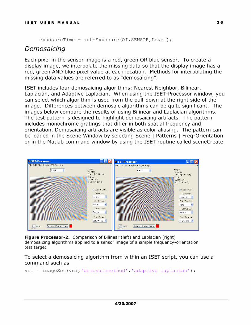
exposureTime = autoExposure(OI,SENSOR,Level);

Demosaicing

Each pixel in the sensor image is a red, green OR blue sensor. To create a display image, we interpolate the missing data so that the display image has a red, green AND blue pixel value at each location. Methods for interpolating the

missing data values are referred to as “demosaicing”.

ISET includes four demosaicing algorithms: Nearest Neighbor, Bilinear, Laplacian, and Adaptive Laplacian. When using the ISET-Processor window, you

can select which algorithm is used from the pull-down at the right side of the image. Differences between demosaic algorithms can be quite significant. The

images below compare the results of using Bilinear and Laplacian algorithms. The test pattern is designed to highlight demosaicing artifacts. The pattern

includes monochrome gratings that differ in both spatial frequency and

orientation. Demosaicing artifacts are visible as color aliasing. The pattern can be loaded in the Scene Window by selecting Scene | Patterns | Freq-Orientation

or in the Matlab command window by using the ISET routine called sceneCreate

Figure Processor-2. Comparison of Bilinear (left) and Laplacian (right)

demosaicing algorithms applied to a sensor image of a simple frequency-orientation

test target.

To select a demosaicing algorithm from within an ISET script, you can use a command such as

vci = imageSet(vci,'demosaicmethod','adaptive laplacian');


4/20/2007

You can set the demosaicing method to the standard Matlab sub-routines provided

in ISET, or to a custom Matlab demosaicing algorithm that you provide. The arguments for the custom demosaic routine should be

demosaicedImage = myDemosaic(imgRGB,SENSOR);

In this case imgRGB is an RxCxW image representing the row (R) by col (C) SENSOR data from W-color filter types. Data in the individual planes are mainly zero. The demosaic algorithm interpolates the data to return a full RGB (RxCx3)

image that can be displayed.

Please read the code in the routine Demosaic.m to see the general calling convention. Helpful routines for designing demosaic algorithms are located in the

directory “\ISET-2.0\imgproc\Demosaic”.

Color rendering

In a wonderful world, we could copy the sensor RGB values into the RGB values of a display controller and render an accurate image. While the world we live in is

wonderful in many respects, this is not one of them. Copying sensor RGB directly to display RGB will not produce a high quality output.

There are many algorithms to transform sensor RGB data into display RGB. We refer to the entire process of transforming sensor color data to display data as “Color rendering.”

Many (but certainly not all) color rendering algorithms can be divided into three parts. The literature is inconsistent in naming the three stages of this process. We are consistent; we apologize if we are not consistent with the usage you have

learned.

First the sensor data are transformed into a calibrated color space. We call this stage “Color conversion.” Second, the data are processed within this space to

enhance contrast and improve appearance. We call this, “Color processing.” This stage includes algorithms such as color balancing, as well as contrast or brightness

enhancement. Third the image data are converted into a display space. We call this “Display rendering.” This stage includes algorithms such as gamut-mapping

(accounting for the fact that the display has a limited gamut).

There are many possible color conversion algorithms; we implement two types of one basic (3x3 matrix) approach through the ISET-Processor window. In the next

section, we describe the ISET color rendering process that can be controlled from


4/20/2007

the ISET-Processor window. It is also possible to substitute your own custom color

rendering process using ISET scripts.

Color conversion

First, we describe a means of identifying a color conversion matrix that is based on

a calibrated target, the Macbeth Color Checker illuminated under a particular illumination (D65). This method is used when you select “MCC Optimized” under

the Color transform method. Second, we describe a method of entering a color conversion matrix manually. You can do this by choosing the option “Manual Matrix

Entry.”

MCC Optimized. Because the MCC target and D65 illumination produce a calibrated signal, we can calculate the target‟s effect on the human visual system; say by

calculating the CIE XYZ values for the 24 patches in this target. Let‟s call the 24x3 matrix of XYZ values for this target, tXYZ.

Next, we can use ISET to simulate the sensor responses to this same target. Call

the 24x3 matrix of simulated sensor responses to this target simRGB.

We can compute a color conversion matrix by finding the 3x3 matrix, M, that is the least-square solution to the equation tXYZ = simRGB*M. ISET stores this color

conversion matrix and uses it to transform the simulated RGB values into a calibrated color space (in this case the CIE XYZ).

It is possible to perform this same calculation in a variety of ways. For example, we may decide to transform the data into another calibrated space (e.g., the Stockman

human cone fundamentals). Or we might decide to simply leave the color data in

the original sensor space (in which case M is the identity matrix).

Manual Matrix Entry. You may decide to implement a different method for finding the color matrix. For example, you may not want to use the surfaces in the Macbeth Color Checker to determine the conversion matrix because these surfaces

were not designed for this process. Instead, you might use a method like the one

above to derive a different 3x3 matrix, M. In that case, you can simply enter the matrix you designed into the processor window by using the “Manual Matrix Entry”

option.

When you choose this option, the “Internal color space” pull down and the “Color Balancing” pull down are removed. We assume that the matrix you are entering is

precisely the one you wish to use to convert from the sensor values to the display result.


4/20/2007

Color processing

There is a limitless set of possibilities for processing enhancing the color data.

Smoothing, sharpening, contrast and saturation enhancement, and brightening are all possible to include in this stage of the processing. This broad array of processing

algorithms is far too complex to explore effectively within this simulation pipeline.

The ISET-Processor window does offer help, however, with one type of color

processing: Color balancing. The goal of color balancing is to transform the image data so that the displayed image appears similar to the original image. Because the

illuminant in the original image and the implicit illuminant on the display may differ, simply reproducing the same XYZ values on the display will not produce the same

color appearance. If you wish to make the rendered image appear similar to the original, when the rendered and original are viewed in different contexts, you must

transform the XYZ data to compensate for the illumination difference.

The literature on color balancing is quite large and includes many different types of

algorithms, of varying complexity. ISET 2.0 includes several popular methods for color balancing. It includes the “Gray World” algorithm which scales the image R, G

and B pixel values so that the mean R, mean G, and mean B values are equal. This

method can be applied directly to the linear sensor values (in which case the user selects the “Sensor” option in the choice of color space), the XYZ transformed pixels

values (select “XYZ”), or the Stockman transformed pixel values. You can, of course, add other color space transformations.

ISET also includes a variant of the “Gray World” algorithm (which we call the “White World”) which scales the image R, G and B pixels values so that the highest R, G

and B values are equal. Again, you select the color space in which the scaling occurs.

Image Quality Metrics

There is no single way to evaluate the quality of an image. The image may have good contrast, but poor color balance. It may be in sharp focus but too

dark. Some portion of the image may look great; another may have motion blur. Hence, there can be no single measure of image quality.

The ISET-Processor window includes a variety of tools to assess image quality. These can be invoked from the “ISET-Processor | Analyze” pull-down window.


4/20/2007

In this section, we define the basic image quality measures, and we emphasize

those that have a basis in international standards.

Spatial resolution and the MTF

The International Standards Organization (ISO) has adopted a standard (ISO

12233) to evaluate the sharpness of a digital imaging system. The idea is based

on measuring the contrast along the edge of a slanted bar target. You can perform this analysis entirely from the ISET-Processor window by first selecting

“ISET-Processor | Analyze | Create Slanted Bar”. This will produce an image of the slanted bar target using the current settings in the optics, sensor and

processor window. Figure Processor-3 is an example of a slanted bar image.

Figure Processor-3. A slanted bar image created using the “ISET-

Processor | Analyze | Create Slanted Bar” pull-down menu. When using

this pull-down, the system uses the current optics and sensor settings.

Alternatively, you can create a slanted bar image explicitly, beginning in

the scene window and experimenting with optics, sensor and image


4/20/2007

processing settings.

The ISO 12233 standard then has the user select a region from the edge of the bar. Using the slope across the edge points, the standard computes the spatial

modulation transfer function in each of the color channels and for a luminance channel made by adding together the color channels. You can invoke this metric

by selecting “Image-Processor | Analyze | ISO 12233 (Slanted Bar)”. After you invoke this command, you choose the rectangular region. An ISET graph

window, defining the MTF responses to the different color channels, will be

produced.

0 50 100 150 200 250 300 350 4000

0.1

0.2

0.3

0.4

0.5

0.6

0.7

0.8

0.9

1ISO 12233

Spatial frequency (cy/mm)

Con

trast

red

uct

ion (

SF

R)

Nyquist = 178.57

Mtf50 = 122.56

Percent alias = 27.77

Figure Processor-4. The output of an ISO 12233 analysis for particular sensor and

image processing configuration. The graph shows the contrast reduction as a

function of spatial frequency for each of the three channels, as well as for a

luminance channel (black line). In this particular processing configuration, the green

and blue channels (but not the red) were scaled by the color balancing algorithm.

The demosaicing algorithm was the Laplacian. The optics and pixel size were poorly

chosen, so that there is considerable spatial aliasing. The small vertical line (at

178.57 cycles/mm)indicates the Nyquist sampling frequency.

A more detailed description of the metric process is provided in the ISET Application Notes “How to Calculate the System MTF”.

MCC Luminance noise

The visibility of luminance noise can have a big effect on perceived image quality. The pull-down menu “ISET-Processor | Analyze | Color and Luminance |

MCC Luminance noise” measures the system luminance noise in a Macbeth Color Checker (MCC).


4/20/2007

To perform this analysis, you should create a Scene containing an MCC. Once you have set up the optics, sensor and processing parameters, you can invoke

“ISET-Processor | Analyze | Compute from Scene” to generate a display of the MCC.

Next, select the MCC Luminance noise pull-down menu. You will be asked to identify the four corners of the MCC target by left-clicking on the outer corners

of the white, black, blue/cyan and brown targets. (You can use the backspace key to undo a point). Click the right button when you are satisfied with the

points. (Make sure you clicked in the proper order, as indicated in the text message of the window).

This algorithm identifies the central position of the gray-scale sequence at the

bottom of the MCC. The percent luminance variance in each of the patches is calculated and plotted in an ISET graph window.

1 1.5 2 2.5 3 3.5 4 4.5 5 5.5 60

1

2

3

4

5

6

Gray patch (white to black)

Perc

ent

lum

inan

ce n

ois

e (

std

(Y)/

me

an

(Y))

x10

0

Figure Processor-5. The percent luminance noise in the six patches of the MCC

gray-series. In this case, there is very little noise in the white patch, and nearly 6

percent luminance variance in the black patch. The horizontal line, drawn at 3

percent, marks the visibility threshold for luminance noise. Hence, only the noise in

the very darkest patch will be visible.

MCC Color metrics

This image quality metric uses the CIELAB color metric to calculate how accurately the color conversion method reproduces the colors in a Macbeth Color

Checker (MCC). Begin by creating a scene of an MCC rendered under a D65


4/20/2007

illuminant (“Scene | Scene | Macbeth Charts | D 65”. After adjusting the optics,

sensor and image processing settings, choose the pull-down “ISET-Processor | Analyze | Compute from Scene”. This produces the MCC image in the ISET-

Processor window.

Next, invoke the pull-down menu “ISET-Processor | Analyze | Color and Luminance | MCC Color Metrics”. The data in the Processor window will be

compared with the exact data one would expect for an MCC under D65 illumination. The calculation assumes that the image white point is equal to the

values measured at the white surface.

-100 0 100-100

0

100

a (red-green)

b (

blu

e-y

ello

w)

CIELAB color plane

0 5 10 150

2

4

6Mean deltaE = 5.58

0 5 100

50

100

Gray patch

L*

Achromatic series

0 0.2 0.4 0.6 0.80

0.2

0.4

0.6

0.8

x

y

Chromaticity (CIE xy)

Figure Processor-6. The “Analyze | Color and Luminance | MCC Color Metrics”

pull-down menu analyzes how accurately an MCC Color Checker (D65 illuminant) is

rendered. The user is asked to select the four corners of the MCC (white, black,

cyan, brown). The image is analyzed and error metrics for the MCC patches are

plotted in the four panels of the window. The graph in the upper left shows the

(a*,b*) color error. The graph in the lower left shows the measured and expected

L* values for the six gray patches. The upper right shows the Eab error histogram.

The graph at the lower right shows the xy chromaticity values. In the upper left and

lower right panels the blue circles indicate the measured value and the small red

lines show the distance from the measurement to the ideal value.


4/20/2007

Metrics window

Not fully implemented


4/20/2007

ISET Programming Guide

ISET is designed to be controlled either by a graphical user interface, or by writing

scripts based on an open-source collection of Matlab routines. Using either method, users can calculate the transformations along the imaging pipeline and measure the

effects of different components in the imaging system. While some tasks can be performed best using the graphical user interface, other tasks, say those that

require looping through parameters or searching, are best approached using scripts.

For a description of the ISET functions, go to

http://www.imageval.com/public/Products/ISET/Manual/Functions.htm

http://www.imageval.com/public/Products/ISET/Manual/Functions.htm


4/20/2007

ISET Scripts and Application Notes

A list of the separate documents containing application notes for various tasks, usually associated with ISET scripts.

Scene High Dynamic Range Spectral (HDRS) Scene Database

The ISET package includes images from our high dynamic range spectral (HDRS) image database. These images are complete spectral

approximations the light radiance field. The full HDRS image database includes a collection of additional images and customized software tools.

This document describes the methodology we used to acquire the data and estimate the spectral radiance for the images in the HDRS database.

Optics ZEMAX Module

Generating distorted image height, relative illumination, optical parameters and PSF data using ZEMAX

Microlens Module

In many digital image sensors an array of microlenses is placed near each pixel aperture on the sensor surface. The position and properties of this

microlens array control two important functions of the optical path from the sensor surface to the photodetector. First, the microlenses concentrate

photons incident within the pixel aperture onto a compact region at the silicon substrate. Second, the microlens array redirects the light path.

Processor Selecting a Color Conversion Matrix

This document gives a step-by-step description of using ISET to calculate a color correction matrix (CCM). The method is based on (a) simulating the

responses to a Macbeth Color Checker under a specific illuminant, and (b)

http://www.imageval.com/public/Products/ISET/Manual/PDF/HighDynamicRangeScenes.pdf

http://www.imageval.com/public/Products/ISET/Manual/PDF/Microlens.pdf

http://www.imageval.com/public/Products/ISET/Manual/PDF/ColorCorrectionMatrix.pdf


4/20/2007

using the simulated sensor responses to derive a 3x3 linear matrix (a

CCM) that can be used for Manual Matrix Entry.

Metrics

Calculating Color Accuracy using the Macbeth ColorChecker This document describes how to use the CIELAB color metric to calculate how accurately the color conversion method reproduces the colors in a

Macbeth Color Checker (MCC).

Calculating the System MTF using ISO-12233 (Slanted bar) ISET implements the ISO 12233 (Slanted bar) method for calculating

system the Modulation Transfer Function (MTF). This document describes a step-by-step procedure for how to perform this calculation.

Measuring the Visibility of Noise with the Minimum Photometric Exposure (MPE)

Spatial Resolution and Sensitivity Tradeoffs

http://www.imageval.com/public/Products/ISET/Manual/PDF/ColorAccuracy.pdf

http://www.imageval.com/public/Products/ISET/Manual/PDF/SlantedBarMTF.pdf


4/20/2007

Glossary and Formulae

.


4/20/2007

Appendix

A. Matlab® Data Conversion Routines

ieXL2ColorFilter: routine to run inside of Matlab® to convert spectral data in Excel spreadsheet into spectral data as a Matlab® file (file.mat).

The data should have wavelength in the first column of the Excel spreadsheet

and sensitivity (or transmissivity) in the subsequent columns (scaled between 0 and 1)

Example: An Excel spreadsheet for a cyan, yellow, magenta filters

Wavelength

(nm)

Cyan (%T) Yellow

(%T)

Magenta (%T)

780.0000 0.6691643 0.9876172 0.9725687

778.8889 0.6628207 0.9883542 0.9718713

777.7778 0.6568444 0.9884193 0.9725651

776.6667 0.6497047 0.9895866 0.9719566

775.5555 0.6430920 0.9885254 0.9713735

774.4445 0.6362457 0.9898154 0.9713428

773.3333 0.6301257 0.9890532 0.9709100

772.2222 0.6228593 0.9891331 0.9707350

771.1111 0.6165825 0.9910802 0.9709256

770.0000 0.6101215 0.9900860 0.9721787

… … … …

… … … …

378.8893 0.1270044 0.2420548 0.5602559

50

Index

A

Analyze · 4

anti-aliasing filters · 20

auto-exposure · 31

Auto-exposure · 35

B

Bayer color filter array · 31

C

CIELAB · 42

Code V® · 23

color conversion · 34

Color conversion · 37, 38

color filter array · 31

Color processing · 37, 39

Color rendering · 37

Color test patterns · 12

Color-balancing · 35

conversion gain · 28

cos4th · 20

D

dark voltage · 28

demosaic · 34

demosaicedImage · 37

Demosaicing · 36

Diffraction-limited optics · 19

Diffuser · 20

Display rendering · 37

dlMTF · 21

E

Edit · 3

electrical noise · 25

energy · 10

Energy2Quanta · 16

etendue · 32

exposureTime · 36

F

faulty pixel replacement · 33

field height · 22

field of view · 12

field of view. · 16

File · 3

filter transmissivities · 32

FOV · 12

G

gainFPNimage · 31

Graphical User Interface

GUI · 1

Gray World · 39

H

HDRS · 14

Help · 4

I

ieCompressData · 10, 18

ieUncompressData · 10, 18

illuminant SPD · 14

illumination functions · 13

image processing pipeline · 34

51

image quality metrics · 35

Image Quality Metrics · 39

Image Sensor Array · 25

imageGet · 33

image-processing pipeline · 33

imageSet · 33, 36

imaging pipeline · 8

indices of refraction of the metal layer · 25

Installation · 5

integrationTime · 31, 35

irradiance · 18, 25

ISA · 30

ISET

Image Systems Engineering Toolbox · 1

ISO 12233 · 40, 41

ISO-12233 · 13

isoplanatic · 22

L

Luminance noise · 41

M

Mackay pattern · 13

Manual Matrix Entry · 38

Matlab® imtool function · 27

MCC Color metrics · 42

MCC Luminance noise · 41

MCC Optimized. · 38

mean scene luminance · 12

microlens · 25

microlens toolbox · 32

N

noise evaluation · 14

O

offsetFPNimage · 31

OI.data · 18

oiCompute · 16, 20, 23

oiCreate · 18

oiDiffuser · 20, 23

oiGet · 18, 19

oiSet · 18

oiWindow · 18

Optics · 18

opticsCos4th · 23

opticsDLCompute · 23

opticsGet · 23

opticsOTF · 23

opticsRayTrace · 23

opticsSICompute · 23

orrelated double-sampling · 31

P

paraxial imaging. · 21

photons · 10

physical units · 27

PIXEL parameters. · 28

pixel response · 30

PIXEL structure · 25

PIXEL variables · 28

pixelCreate · 25

pixelGet · 25

pixelSet · 25

Plot · 3

Processor · 33

Pull-Down Menus · 3

Q

Quanta2Energy · 16

R

radiance image · 10

Ray trace optics · 22

read noise · 28

RGB Images · 15

S

Scene · 9

Scene data · 9

SCENE properties · 12

SCENE.distance · 10

SCENE.spectrum · 10

SCENE.wAngular. · 10

sceneCreate · 9, 12, 13

sceneCreateMacbeth · 13

sceneGet · 9, 10, 11

sceneSet · 9

sceneSetEditsAndButtons · 12

sceneShowImage · 12

sceneWindow · 11

Sensor · 25

sensor array · 25

SENSOR array · 30

SENSOR data · 26

sensor metal layers · 25

sensor noise · 30

SENSOR parameters · 29

SENSOR structure · 25

Sensor window · 26

SENSOR.quantization · 31

sensor{Set,Get} · 25

sensorCreate · 29

sensorCreate. · 25

sensorData2Image. · 26

52

sensorGet · 25

sensorImageWindow · 25, 26

sensorSet · 30, 35

sensorSet. · 25

Session variable · 3

Session Window · 8

Shift-invariant optics · 21

sigmaGainFPN · 31

sigmaOffsetFPN · 31

signal-to-noise (SNR) ratio · 29

simulation pipeline · 18

slanted bar target · 40

Spatial resolution and the MTF · 40

Spatial test patterns · 13

spectral characteristics of the filters · 25

sRGB · 34

Stockman · 39

Systems Approach · 2

V

vcImageCreate · 33

vcSESSION · 7

visibility threshold for luminance noise · 42

voltage swing · 28

W

well capacity · 28

White World · 39

X

XYZ · 39

Z

Zemax® · 23

zoom · 27

iset manual

Documents

introduction iset

iset scripts

iset programming guide

image systems hardware

imaging optics

systems approach

graphical user interface

s e t u s e r