1

Is there a Glass Ceiling or Sticky Floor in India? Examining the Wage Gap across the

Wage Distribution

Abstract

This paper tries to give evidence of „Glass Ceiling‟ or „Sticky floor‟ in labour market

in India. Glass ceiling is a situation where the advancement of a person within the hierarchy

of an organization is limited by deliberate design; and sticky floor is the situation where

otherwise identical men and women might be appointed to the same pay scale or rank, but

women are appointed at the bottom and men further up the scale. This study tries to analyze

gender, caste and religion based discrimination in both regular and casual labor market in

India. The data for the study is collected from National Sample Survey Organization (NSSO),

India. We have used data of employment and unemployment survey in 2004-05 (61st round)

and recent 2011-12 (68th

round). The Blinder-Oaxaca decomposition method and Machado

Mata Melly decomposition method are being used to decompose the wage gap at different

quantile of wage distribution along with mean. The findings show a declining trend of gender

wage gap from 2004-05 to 2011-12. The decline in endowment difference has largely

contributed to decline in raw wage differentials. The gender discrimination is widening over

the years, because the percentage contribution of coefficients to the raw wage difference is

showing an increasing trend. We observe evidence of „sticky floor‟ in both regular and casual

labour market in India. The evidence of sticky floor implies that women at the lower end of

the overall wage distribution experience larger wage gaps compared to women at the upper

end. The wage gap between Scheduled Caste and Non Scheduled Caste casual workers is

increasing throughout the wage distribution and it is more at the upper tail. The workers from

lower caste groups experience „glass ceiling‟ in casual labour market. It is due to

occupational segregation in labour market. The Scheduled Caste workers are still confined to

traditional caste occupations or occupations with low returns. The policy should be in favor

of breaking this hierarchy of occupation in labour market. As far as caste based

discrimination is concerned, we found that the percentage contribution of characteristics

(endowment) to raw wage difference has increased over the years, except in casual worker‟s

lower wage distribution. It is important to note that the large endowment difference implies

prevalence of pre-market discriminatory practices in India. The average earnings of Muslims

are comparatively lower than that of NonMuslims in regular labour market. Out of total raw

wage gap between Muslim and NonMuslim wage gap in regular labour market, almost 70

percent is on account of endowment difference. There is a need for continued government

policies aimed at education and skill building for the Scheduled Castes and Muslim people.

2

1 Introduction

The existing literature gives utmost importance to mean wage gap across different

socio-religious groups in labour market. But this kind of studies neglects the larger and

smaller gap that lies in low wage and high wage distribution. There are possibilities of

accelerating wage gap at lower tail and upper tail of the distribution. This gives rise to the

phenomenon of „Glass Ceiling‟ and „Sticky floor‟ in labour market. Glass ceiling is a

situation where the advancement of a person within the hierarchy of an organization is

limited by deliberate design; and sticky floor is the situation where otherwise identical men

and women might be appointed to the same pay scale or rank, but women are appointed at the

bottom and men further up the scale. Some of the existing studies look at this issue from

gender perspective. However, in Indian context, the analysis can be extended to caste and

religion perspective. There are large numbers of cases, where workers belonging to backward

communities and Dalit are the worst victim of discrimination in labour market. Their access

to high profile formal sector jobs is quite limited. The purpose of this study is to do a

distributional level analysis of wage structure in both regular and casual labour market in

India. We attempt to empirically test the hypothesis of „Glass Ceiling effect‟ and „Sticky

floor effect‟ in labour market.

The motivation of the study is to answer the following questions: Is there any

significant wage gap across gender, caste and religious groups in regular and casual labour

market in India? Does „Glass Ceiling‟ or „Sticky Floor‟ exist in labour market? Why such

phenomenon occurs?

This paper is organized in the following fashion. The section 1, gives introduction of

the study. The brief review of literature is given in section 2. The sources of data and

methodology applied in research are given in subsequent section 3 and 4. The section 5

provides the empirical results and discussion, which is divided into two sub sections i.e.

descriptive results and Econometric analysis. Finally section 6 concludes the study.

2 Brief Review of Literature

There are many national and international literatures that try to analyze the concept of

„Glass Ceiling‟ and „sticky floor‟ in labour market. The first attempt to define „Glass ceiling‟

in Sweden was done by Albrecht et al. (2003). They found that gender wage gap is increasing

throughout the wage distribution of workers. Particularly wage gap accelerates at the upper

tail of the distribution that can be termed as presence of glass ceiling effect. Even after

controlling for certain variables like gender difference in age, education, sector, industry and

occupation, the results give strong evidence of glass ceiling effect in Sweden. The wage gap

3

at top of the distribution is mostly on account of differential reward to characteristics (i.e.

discrimination) in labour market. The similar study was done by De la Rica et al. (2005) for

Spain by using ECHP (1999) data. They have divided the sample into highly educated and

lower educated workers. For highly educated (college/tertiary education) workers, in line

with the conventional glass ceiling hypothesis, the gender wage gap increases as we move up

the distribution. However, for less educated (primary/secondary education) workers, the

gender wage gap decreases as we move up the distribution. This gives rise to the floor

pattern. This is due to the practice of statistical discrimination by employers and as a

consequence lower educated female participation is less in labor market.

Following the above mentioned studies, a cross country analysis on sample eleven

European Union countries was done by Arulampalam et al. (2006). In order to facilitate cross

country comparison, they define the existence of „Glass ceiling‟, if 90th

percentile wage gap

is higher than the estimated wage gaps in other parts of the wage distribution by at least 2

percentage points. The „Sticky floor‟ is said to exist if 10th

percentile wage gap is higher than

the 25th

percentile wage gap by at least 2 percentage points. In other words, the phenomenon

of widening wage gap at the bottom of the distribution can be termed as „Sticky floor‟ in

labour market. The findings of the study reveal that the estimated gender wage gap is higher

at the top of the wage distribution, suggesting that glass ceilings are more prevalent than

sticky floors. The gender wage gap also differs significantly between public and private

sector in all countries. The private sector exhibits very large wage gaps compared to public

sector. The estimated results of gender wage gap vary among EU countries due to

heterogeneity in institutions among them.

Chi, Wei & Li, Bo (2008) has made an attempt to analyze gender pay gap in Chinese

urban labour market by using UHS (1987-2004) nation-wide data. They found evidence of

„Sticky floor‟ effect in labour market. The gender differences in the return to labour market

characteristics (discrimination effect), contribute to the increase in the overall gender pay

gap. The sticky floor effect may be associated with low paid female production workers,

having lower educational attainment and working in non-state owned enterprises. The gender

wage gap in French profit and nonprofit sectors was done by Etienne and Nancy (2007). They

suggest that Glass Ceiling‟ effect is lower in nonprofit sector than in profit sector. The low

rate of discrimination in nonprofit sector acts as a means to maintain and enhance intrinsic

motivation of the workers.

In Indian context, Khanna (2012) has made the first attempt to analyze „Glass Ceiling‟

and „Sticky floor‟ among regular worker using National Sample Survey (2009-10) data. The

4

findings give evidence of „Sticky Floor effect‟ and it is driven by discrimination in labour

market. The discrimination contributes almost 80 percent of gender wage differential in

regular labour market in India. Subsequently, Agarwal (2013) has studied gender related

wage differentials in rural and urban India. The findings give evidence of the glass ceiling

effect in the rural sector and evidence of the sticky floor effect in the urban sector. The result

of the counterfactual decomposition revealed that labour market discrimination against

women is comparatively higher at the lower end than at the upper end of the distribution.

Azam (2009) has studied wage structure in urban India by applying quantile

regression method. The findings show that there is an increase in real wages rate throughout

the wage distribution during 1983 to 1993-94; and the increase in real wage rate in the upper

half of the distribution occurs during post-liberalization phase from 1993-94 to 2004-05. It is

also associated with increasing return to tertiary and secondary education. He suggests that

wage inequality in urban India may increase further in near future as more workers get

tertiary education. The subsequent study of Azam (2010) using NSS (2004-05) data revealed

that the raw gender wage differential between public and private sector is positive across the

distribution, irrespective of area of residence. The public-private wage differential on account

of difference in observed characteristics (covariate effect) is less at the lower part of the

distribution but its contribution increases at the upper part of the distribution. Recently

Sengupta and Das (2014) tried to analyze gender wage discrimination across social and

religious groups in India. It is found that discrimination is more severe for women workers

belonging to backward ethnic groups as compared to other women workers.

Madheswaran (2008) has analyzed caste discrimination in both public and private

sector in India by using NSS (2004-05) data. He found that wage gap on account of

discrimination is comparatively higher in private sector than that in public sector in the entire

distribution except in lower wage distribution. Subsequently, Madheswaran (2010) paper has

done a descriptive analysis in order to observe the gender wage gap in regular urban labour

market. He found evidence of „Glass Ceiling‟ and „Sticky Floor‟ in labour market. The raw

gender wage gap in the bottom percentile is very high in public sector than that in top

percentiles. However, raw gender wage gap in private sector is comparatively higher than

that in public sector in almost all the percentiles groups.

From the above review of literature, we observe that quite a few studies have done a

distributional analysis of wage structure in India. One can do a separate analysis for gender,

caste and religious groups in labour market. This kind of study has greater relevance in Indian

context, because female, lower caste and religion minorities (especially Muslims) are

5

supposed to be in disadvantageous position in labor market compared to their counterparts.

The observation of the changes of this pattern over the period of time has important policy

contribution. Occupational segregation is the form in which the glass Ceiling effect is

manifested in labour market. We are trying to analyze the effect of occupation on wages

through cross classification of workers by gender, caste and religious groups.

3 Sources of Data

The present study uses secondary data at aggregate level. Data for the study is

collected from the National Sample Survey Organization (NSSO), India. For the purpose of

the study, NSS employment and unemployment survey in 2004-05 (61st round) and recent

2011-12 (68th

round) data is used. The 61st round of NSS was conducted during July, 2004 to

June, 2005. It covered 1,24,680 households (79,306 in rural areas and 45,374 in urban areas)

and enumerated 6,02,833 persons (3,98,025 in rural areas and 2,04,808 in urban areas). The

68th round of NSS was conducted during July 2011 to June 2012. It covered 1, 01,724

households (59,700 in rural areas and 42,024 in urban areas) and enumerated 4, 56,999

persons (2, 80,763 in rural areas and 1, 76,236 in urban areas). In this survey, the sample of

households is drawn based on a two-stage stratified random sampling procedure. The first

stage units are the census villages and urban blocks and the second stage comprises the

households in these villages and urban blocks. This survey provides information at household

and individual level. The detailed information regarding survey and the aggregate estimates

are given in NSSO.

The sample of individuals is divided into two mutually exclusive categories using

current daily status: (i) non-wage earners (i.e., non-participants in the labour market, the self-

employed and the unemployed) and (ii) wage earners. Our study proposes to include wage

workers of 15-65 age groups. The survey provides information on both household and

individual characteristics. The data relating to human capital, demographic and job

characteristics of workers are readily available. The available data on human capital

characteristics include age, education; data relating to demographic characteristics include

gender, social group, religion, marital status, location (rural/urban), region (north, south, east,

and west); data relating to job characteristics include industry, occupation (7 categories such

as, administrative, professional, clerical, service, farmer, production, elementary occupation),

sector (Public/Private).

The daily wage rate of workers is calculated taking into consideration the total wages

in cash and kind receivable for the work done in the reference week by the total number of

days reported working in wage work in that week. The wage distribution is trimmed by 0.1

6

percent at the top and bottom tails in order to get rid of outliers and potentially anomalous

wages at the extreme ends of the distribution. Our estimation of wage gap is done by using

real daily wages data. The real daily wages are calculated by deflating the nominal daily

wages to 2001 prices. The CPI (AL) and CPI (IW) are used for deflating rural wages and

urban wages respectively (Labour Bureau, various years). The Consumer Price index data is

collected for states like Andhra Pradesh, Assam, Bihar, Gujarat, Haryana, Himachal Pradesh,

Jammu and Kashmir, Karnataka, Kerala, Madhya Pradesh, Maharashtra, Orissa, Punjab,

Rajasthan, Tamil Nadu, Uttar Pradesh and West Bengal; and our empirical analysis

comprises sample of those 17 major states of India.

4 Methodology of the Study

Following the human capital theory, we have used the Mincerian earning function in

our estimation. The specification of the model is given below:

Log Wi = βj Sji + δ1 Ti + δ2 Ti2 + other variables,

i=1….N

The dependent variable in the wage function is logarithm of real daily wage rate (W)

and S is the number of years of schooling, T stands for age of workers, T2 refers to age square

that captures the concavity of the age-earning profile. The coefficient β estimates the rates of

return to schooling (only if there is no ability bias). For estimating augmented earning

function, we have added gender, caste, religion, marital status, public sector, regions, and

occupations as explanatory variables. For creating gender, caste and religion dummy, we

consider male, NonSC and NonMuslims as our comparison category. We estimate three

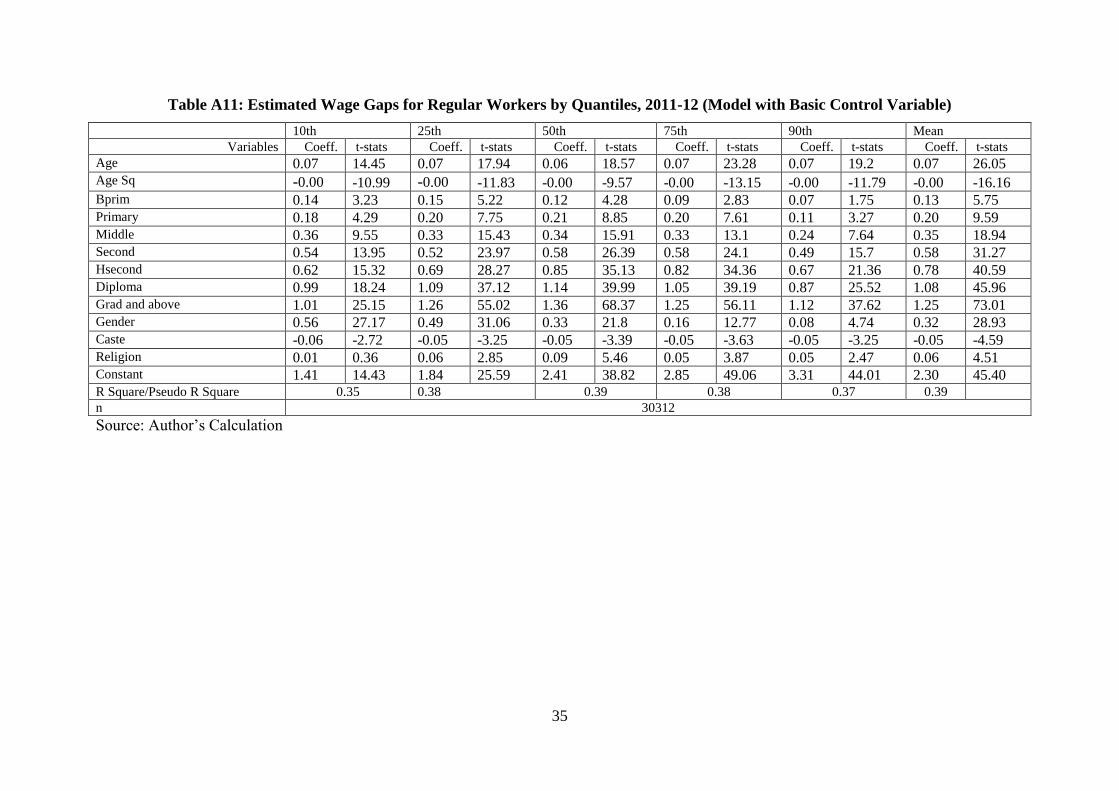
different model specifications. In Model 1, we incorporate basic control variables like age,

agesq, level of education, gender dummy, caste dummy and religion dummy as explanatory

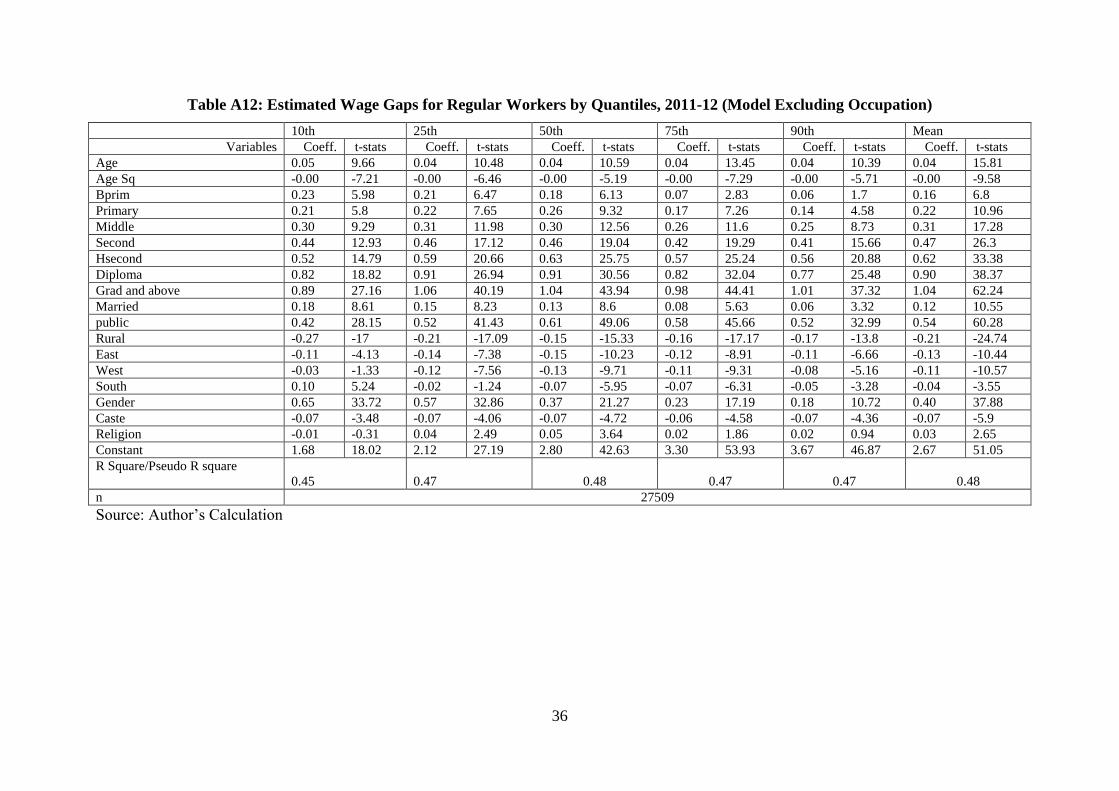
variable. In Model 2, we estimate augmented Mincerian earning function excluding

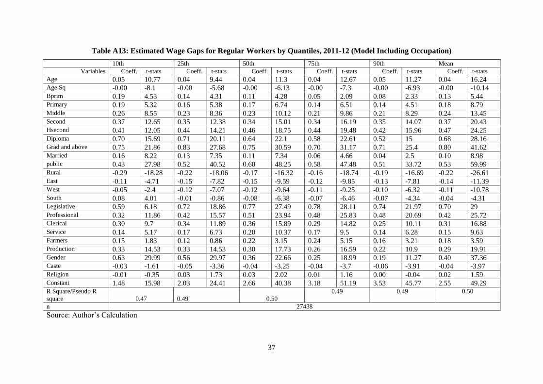
occupation dummies. In model 3, we account for the potential effects of occupation dummies

on wages. The most important result to be analyzed is those from the Model 2, where

occupation dummies are excluded. The reason is that, a comparison of the estimated wage

gap between Model 2 and Model 3 allows us to distinguish the magnitude of the „Glass

Ceiling‟ effect from the „Pure wage discrimination‟ (Albrecht et al. ,2003). In the model 3,

where we include occupation dummies, we interpret the wage gap as „pure wage

discrimination‟. It means within the same occupation and for the same observable individual

characteristics, male/Non SCs/NonMuslims employees are better paid than their counterparts.

7

In order to capture occupational segregation, we exclude occupation dummies from the

model 2.

However, Mincerian earning function suffers from many estimation issues. There lies

data limitation. For example, innate ability, socio-economic background of the individual and

quality of schooling though affect earnings of the individual substantially but we don‟t have

exact data on these factors (Bennell, 1996). This leads to the problem of „Omitted Variable

Bias‟. However, Griliches (1977) found that ability bias need not always positive. In this case

allowing ability as an additional variable when schooling is treated symmetrically will lead to

measurement error and ability will be correlated with the disturbance term. If individual‟s

ability and educational attainment are correlated then estimation will give biased results.

Another important estimation issue is the sample selection bias because of lack of

representative sample. While collecting data on wage rate of working women, it is found that

working women aren‟t the randomly selected sample of all female population. So by using

that data for estimating returns creates sample selection bias. Endogeneity is another problem

comes in earning function because education is an endogenous variable but schooling is an

exogenous variable. In this study, we use level of education as a proxy of schooling.

In this paper, we do not address selection into wage labor market for following

reasons. First, the technique required to correct for selectivity bias in quantile regression

model is less well developed. Second, even if one could adequately address non-random

sample selection, we are only interested in describing the wage distribution conditional on

being in regular or casual employment.

The present study applies both OLS and quantile regression method. The issue of

unequal rates of return to education across quantiles is done in our analysis. In order to

decompose wage gap into explained and unexplained component, we have applied Oaxaca-

Blinder decomposition method and MMM decomposition method.

4.1 Quantile Regression Method

This study applies quantile regression method to analyze wage gap at different

quantiles of the conditional wage distribution. This method was introduced by Koenker and

Bassett (1978). From methodological point of view also quantile regression is better than

OLS. This method reduces sensitivity to outliers. It is more efficient when the error term is

not distributed normally. This method allows us to examine the effect of each of the

covariates along the entire wage distribution, thus give different parameter estimates at

different points of the distribution. The merit of Quantile Regression (QR) over Ordinary

Least Square (OLS) is that we can estimate the marginal effect of a covariate (e.g. gender)

8

on log wage ( ln W) at various points of the wage distribution and not only at the mean. It

helps in addressing the issue of within group inequality. The quantile regression model in the

form of a wage equation can be stated as follows:

iii xw 'ln (1) 0)( ii xE

The assumption of quantile regression model is that conditional quantiles of the dependent

variable ln wi is linear in covariates Xi. Here Xi represents individual characteristics. The th

quantile of the conditional distribution is given by

')(ln iii xxwQ )10(

For a given , the estimate of β solves the following minimization problem (Koenker &

Basset, 1978; Buchinsky, 1998) given below:

}ln)1(ln[1

{min '

ln:

'

ln: ''

i

XWi

ii

XWi

i xwxwn

iiii

It can also be written as:

n

i

in 1

)(1

min

Where, )( is the check function.

)( = ,)1( 0

, 0

We estimate heteroscedasticity corrected standard error by using Machado-Santos

Silva (2000) test for heteroscedasticity. The coefficients of the quantile regression can be

interpreted conceptually in the same way as in the OLS regression. However, incorporating a

gender, caste and religion dummy in the model allows only intercept changes not the slope. It

assumes similar wage structure for male and female, SCs and Non SCs, Muslims and

NonMuslims. In this type of single equation model, the returns to characteristics, or the way

in which the labour market values these characteristics (such as experience, education) are the

same for the two groups. Due to this limitation of applying quantile regression in pooled

sample, we have to go for Oaxaca-Blinder and MMM decomposition method.

9

4.2 Estimation of Private Returns to Education

We calculate private returns to education from our estimated coefficient of Mincerian

earning function. Marginal rates of return to schooling can be defined as the percentage

change in earnings resulting from one more year of schooling. We can estimate average

returns to education to each education level (rj) by using the following formula:

)(

)(

1

1

jj

jj

jSS

Where j = primary, middle, secondary, higher secondary and graduate school, βj is the

coefficient of jth education level in the wage regression models and Sj the years of schooling

at jth

level. (Sj-Sj-1) is the difference in years of schooling between jth

and (j-1)th

levels.

The rate of return to primary education is estimated as follows:

prim

prim

primY

r

where,

primY refers to the years of schooling at primary level.

In case of quantile regression, the quantile rates of return to education can be

estimated as the derivative of the conditional quantile with respect to education(s):

s

xwQuantr

)(ln

Where x is the set of all explanatory variables used in the model.

4.3 Blinder-Oaxaca Decomposition Method:

The Blinder-Oaxaca (1973) decomposition method involves explaining the wage

earned by a Mincerian wage equation. The wage regression is done for each of the groups

(like male and female, or SCs and Non SCs, or Muslims or NonMuslims). Then the

regression coefficients from the „Male‟ equation are substituted in the estimated „female‟

equation to yield the wages that female would have earned if they had been treated as an

average member of the male community. The difference between this wage and the wage that

female actually receive is the measure of discrimination.

10

This method is used to partition the observed wage gap between an „endowment

component‟ and „discrimination component‟. The endowment component reflects the extent

of differential that arise due to differences in workers‟ characteristics and discrimination

component reflects the extent of effect of unobserved characteristics like ability, family

background etc.

The Gross wage differential can be defined as follows:

Yf

YfYmG

= 1

Yf

Ym (1)

Where, Ym and Yf represent the wages of male and female workers respectively, in the

absence of discrimination, pure productivity differences can be defined as follows:

10

0

f

m

Y

YQ (2)

Where, the superscript denotes the absence of labour market discrimination, the market

discrimination coefficient (D) can be defined as the proportionate difference between G+1

and Q+1. This decomposition can be further applied within the framework of semi

logarithmic earnings equation (Mincer, 1974) and estimated via OLS. One has to estimate a

separate male and female regression for this purpose.

Male Wage Equation: mmmm XY ˆln (3)

Female wage equation: ffff XY ˆln (4)

Where, Yln denotes the geometric mean of earnings and X denotes the vector of mean

values of the regressors.

The equations for decomposition can be written as follows:

)ˆˆ()(ˆlnln fmffmmfm XXXYY (5)

)ˆˆ()(ˆlnln fmmfmffm XXXYY (6)

The first term in the right hand side of equation (5) and (6) can be interpreted as „endowment

differences‟ and the second term is regarded as „discrimination component‟. Generally

studies use either of these alternative decomposition forms (equation 5 and 6) based on their

assumptions about the wage structure that would prevail in the absence of discrimination.

11

This kind of a problem is called “the index number problem”. This method is subject to the

limitation of OLS; because the results give the estimated wage gap at the point of mean.

4.4 Machado Mata Melly (MMM) Decomposition Method

This method was initially developed by Machado and Mata (2005). This method is an

extension of the Blinder-Oaxaca decomposition method, in the sense that instead of

considering difference at the mean of the wage distribution, it identifies the sources of wage

gap at various quantiles of the wage distribution. The Machado Mata (MM) decomposition is

based on the estimation of marginal wage distributions consistent with a conditional

distribution estimated by quantile regression. One can perform counterfactual exercises by

comparing the marginal distributions implied by different distributions for the covariates.

The MM procedure involves four steps:

i. Generate a random sample of size m from a U 1,0 : u1, u2……un.

ii. Estimate m different quantile regression coefficients: iu

0

, i= 1,2,…m.

iii. Generate random sample of size m with replacement from the covariates of (Xi)Ti

=0,

denoted by miiX

1

~

.

iv. m

i

iii uXY1

0

~~

is a random sample of size m from the unconditional distribution

of 0)0( TY .

The latest version of decomposition was developed by Melly (2006). The estimator of

Melly decomposition will be numerically identical to MM decomposition if the number of

simulation used in MM procedure goes to infinity. The mean square error in Melly estimation

is comparatively lesser than the MM estimation. The mean square errors of these two

estimates converge only if simulations in MM become very large. Melly estimator is also

consistent and asymptotically normally distributed. For the th quantile, the Melly

decomposition can be written as:

wcfcfmwm QQQQQQ (2)

Where, wm QQ

is the wage gap estimated from the th quantile of the unconditional

log wage distribution for men and women respectively; and cfQ

is the estimated

12

counterfactual unconditional quantile of the log wage distribution for men created using the

coefficients of women. The decomposition is based on the construction of a counterfactual

distribution of cfQ

which represents the distribution of female wages that would have

prevailed if women were given men‟s labour market characteristics.

In equation (2), in the right hand side, the first term can be interpreted as „effects of

coefficients‟ (discrimination), i.e. difference in the distribution of covariates between the two

groups; and the second term is regarded as „effects of characteristics‟ (endowment), i.e. group

specific returns to these covariates across the distribution.

5 Empirical Results and Discussion

Our empirical analysis is based on both descriptive results and econometric analysis.

The descriptive results mostly focus on analyzing average wage gap across socio-religious

groups. In the subsequent econometric analysis, we are applying decomposition method in

order to decompose the wage gap into endowment and discrimination component.

5.1 Descriptive Results

We have divided the descriptive results into following sub-sections as follows:

5.1.1 Average Earnings Differentials across Socio-religious Groups

It is important to note that there exists wage gap across gender, caste and religious

groups in both regular and casual labour market in India.

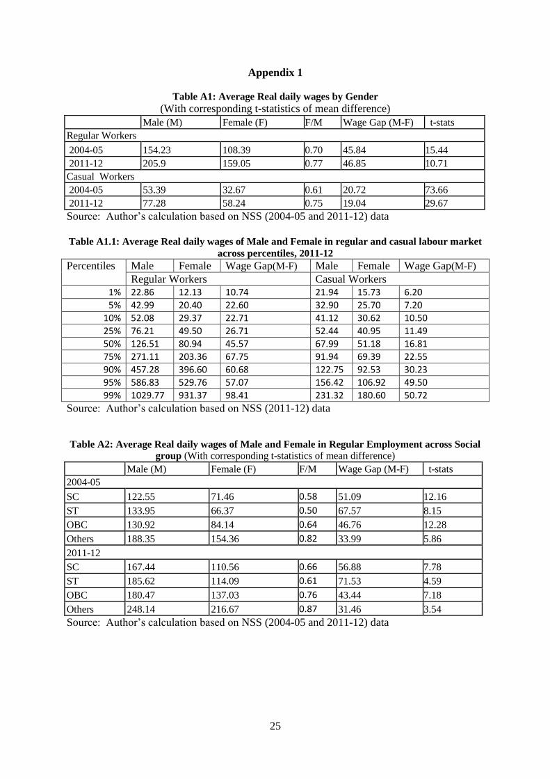
The average real daily wage rate of female is lower than that of male. During the

study period, the gender wage gap shows a slight increase for regular workers from Rs 46 to

Rs 47; whereas for casual workers, it shows a slight decline from Rs 21 to Rs 19. The gender

wage gap shows an increase throughout the wage distribution and it is highest at 99th

percentile. So using average wage rate as a means of measuring inequality across groups

gives misleading picture. The real daily wage rate between regular and casual workers

doesn‟t show any variation at lower tail of the distribution. However, at the upper tail, the

real daily wage rate of regular workers is quite high.

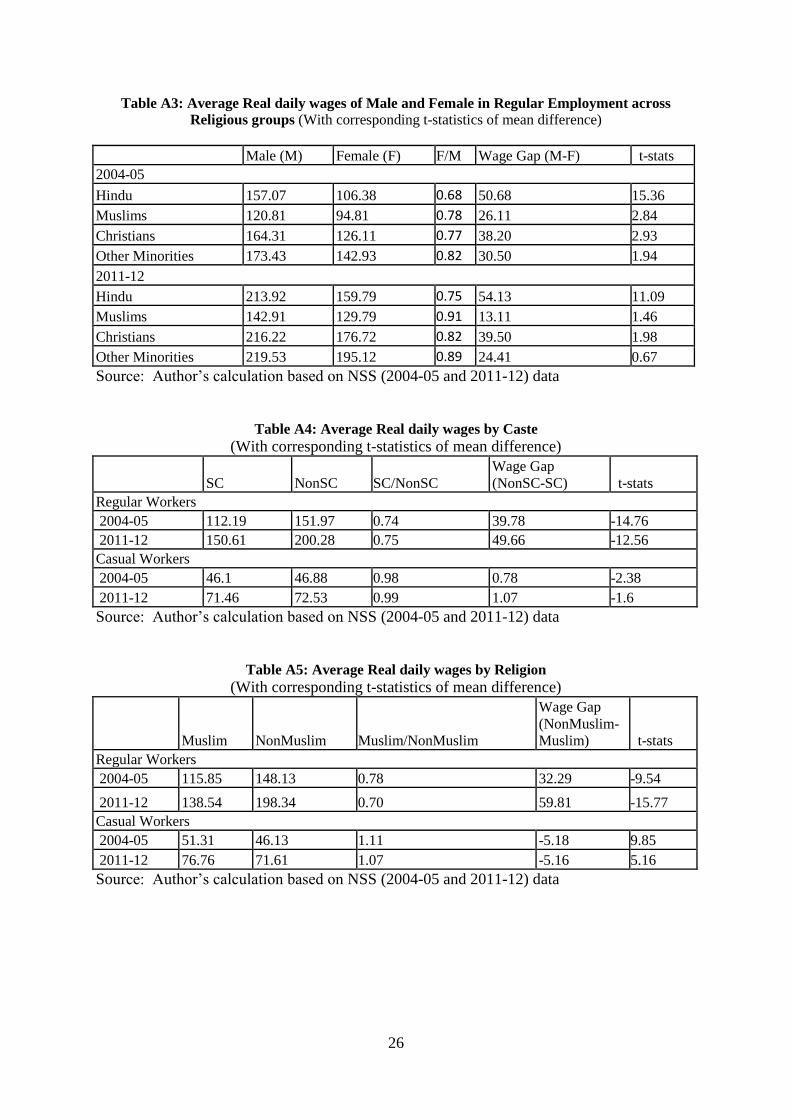
In regular labour market, the gender wage gap among OBC, others, Muslims, and

other minorities shows a decline and for all other cases, gender wage gap shows an increase

from 2004-05 to 2011-12. The regular Scheduled caste workers earnings are not only lower

than their counterparts, but also the Non SC and SC wage gap shows an increase from Rs 40

to Rs. 50 during the study period. However, the average real daily wage rate of SC and Non

SC does not show much variation in casual labour market.

13

Similarly, Muslim regular workers earnings are not only lower than their counterparts,

but also NonMuslim and Muslim wage gap shows an increase from Rs. 32 to Rs. 60 during

the study period. On the other hand, in casual labour market, Non-Muslim and Muslim wage

gap is very less. The summary results are given in Table A1 to A5.

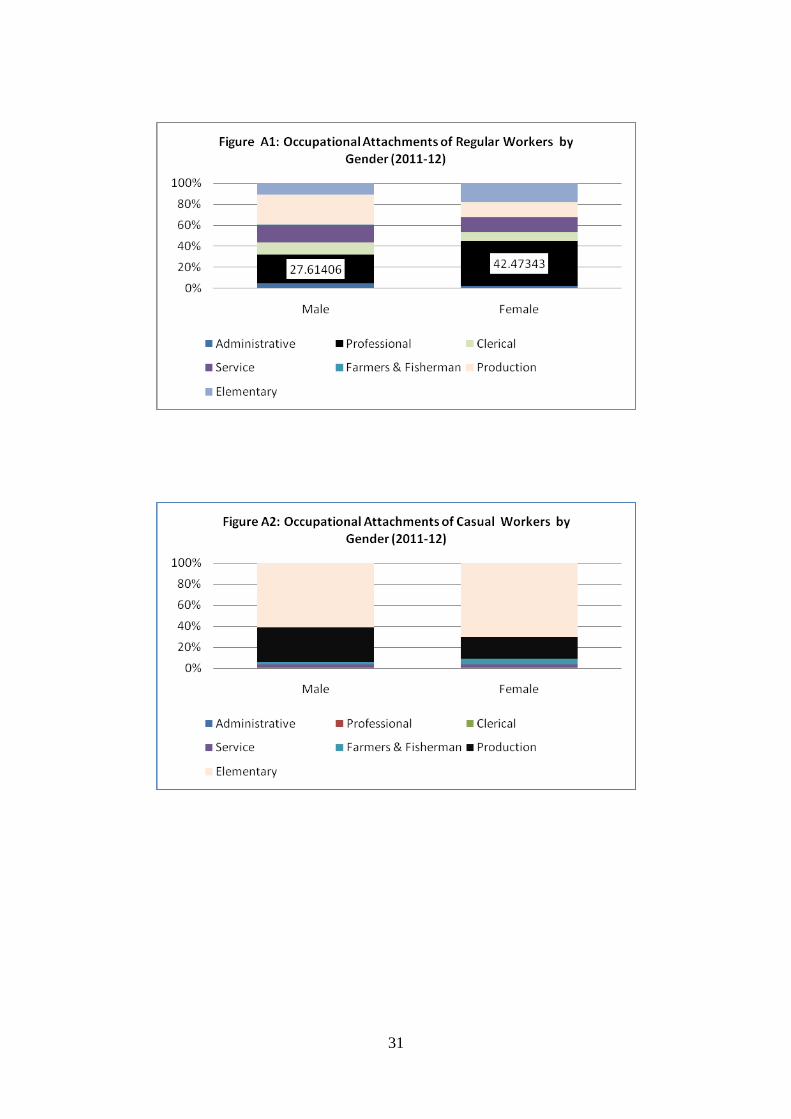
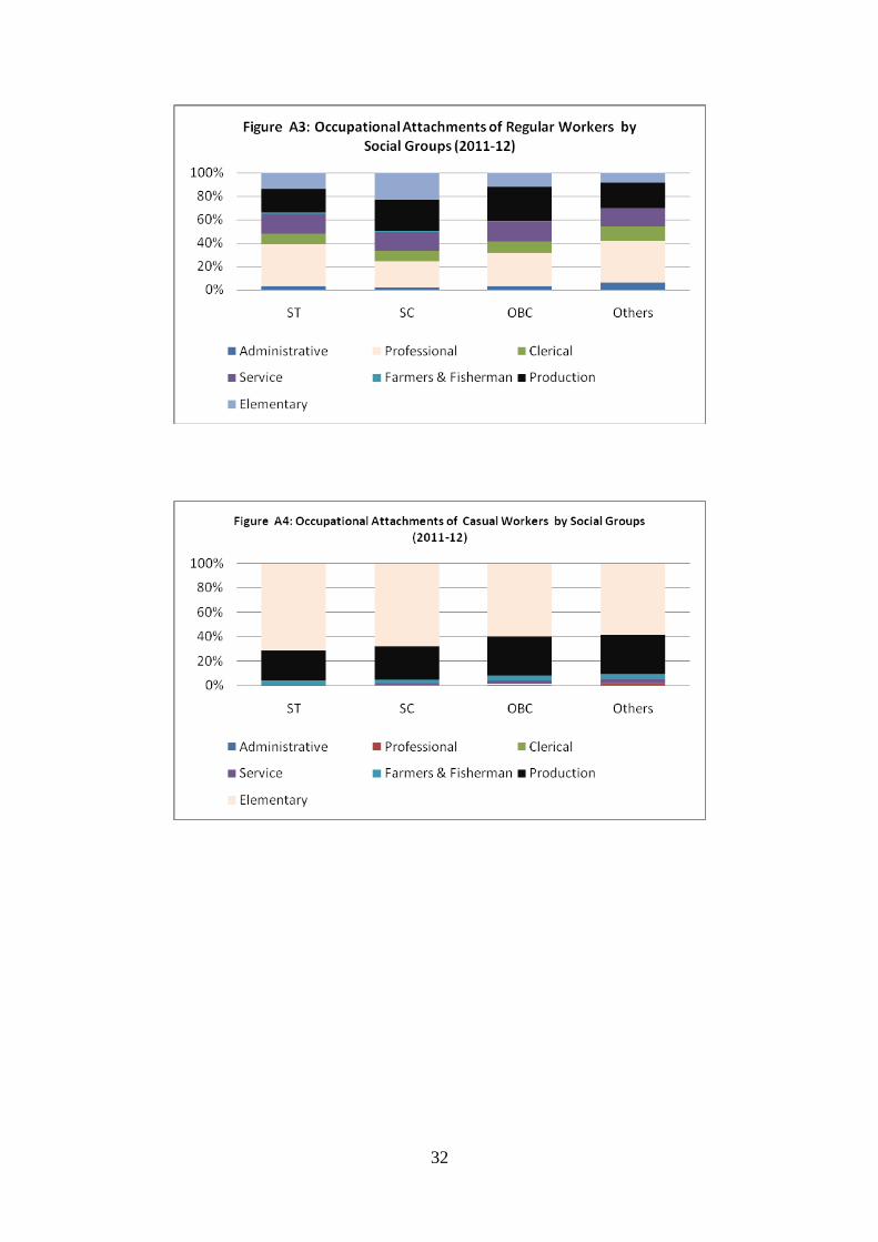
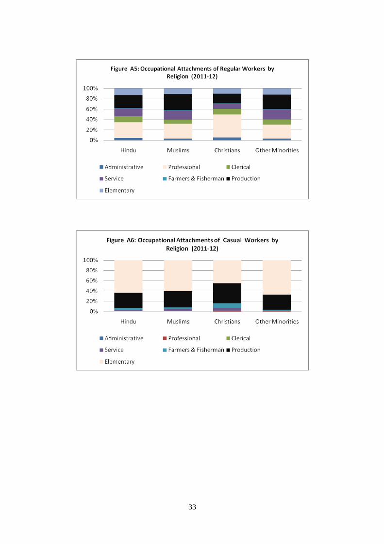
5.1.2 Occupational Distribution of Workers

In Indian labour market, there is persistence of both vertical segregation (within the

same employment type, workers from different social groups may be represented differently

in the hierarchy of positions) and horizontal segregation (workers restricted to their

occupations) between lower caste and upper caste individuals. This affects upward mobility

of workers under the caste hierarchies (Das and Dutta, 2007). It is argued that occupational

segregation is the form in which the glass Ceiling effect is manifested in labour market

(Albrecht et al, 2003).

In regular labour market, concentration of female is highest in professional jobs,

followed by elementary occupation; and concentration of male is highest in production and

trade related activities, followed by professional jobs. On the other hand, in casual labour

market both male and female participation is highest in elementary occupations, followed by

production and trade related activities. The proportion of female as farmers and fisherman is

comparatively higher than that of male in casual labour market. The elementary occupations

include sales and services elementary occupations, agriculture, fishery and related laborers,

laborers in mining, construction, manufacturing and transport.

As per caste based hierarchies of occupation is concerned, in regular labour market,

there about 2 percent to 3 percent of SC/ST workers are concentrated in legislative and

managerial activities compared to 6 percent of general caste workers. It is important to see

that in both regular and casual labour market, SC/ST participation is more in elementary jobs

than their counterparts. These elementary jobs are considered to be in low paid category. On

the other hand, in casual labour market, concentration of OBCs/Others is comparatively more

in production and trade related activities than their counterparts.

Besides, Muslim concentration in production and trade related activities is

comparatively more than that in other occupations. In regular labour market, almost 44

percent of Christians are found to be employed in professional jobs, whereas 29 percent

Muslims are employed in that job. It is important to see that casual employment is quite more

in elementary job that is irrespective of gender, caste and religious groups. The proportion of

workers as farmers and fisherman (skilled agricultural and fishery workers) is declining in

India. The distribution of workers in different occupations is given in figure A1 to A6.

14

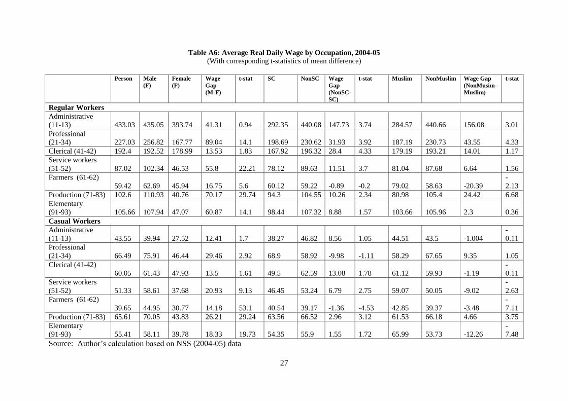
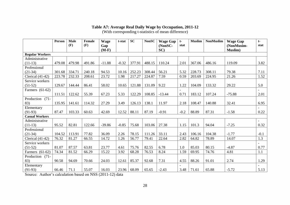
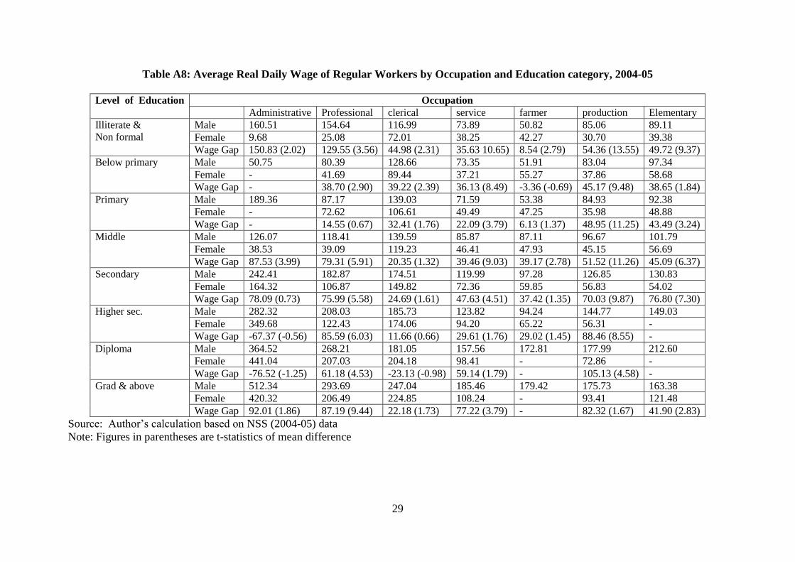
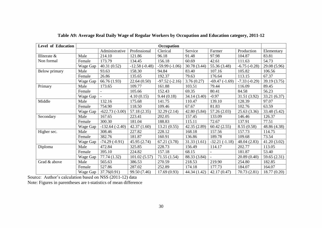
5.1.3 Average Earnings of Workers by Occupation and Education

The average earnings of female workers are lower than that of male workers in almost

all occupations except administrative and managerial activities. During the study period,

there is a rise in female earnings in all types of occupations. The positive relation between

education and earnings is applicable for female workers in professional jobs. During the

study period, the earnings of female from professional jobs are increasing irrespective of

level of education. But female workers in elementary occupations not only earn less but also

their earnings do not increase for higher level of education. In other words, female earnings

from unskilled elementary jobs are comparatively lower than other occupations.

It is important to note that females are crowding in the low paying occupations of the

service and professional categories. Although women represent a large proportion of the

relatively high paying „professionals‟ occupations, most „professional‟ women tend to be in

one of two categories- nurses or teachers which are at the low end of the wage scale

(Madheswaran and Khasnobis, 2007). Similarly, female participation in agriculture and allied

activities is high but female earnings from this occupation are lesser than that of all other

occupations. The gender wage gap is also high in both professional and agricultural activities.

This shows clear case of occupational segregation in labour market. That gives rise to

increasing wage gap at the upper tail of the distribution.

The earnings of scheduled caste workers are lower than that of non-scheduled caste

workers in almost all occupations except in elementary jobs and in regular agricultural

activities. In regular labour market, SCs average earning in elementary occupations is not

only lower than other occupations, but also it shows a decline during the study period. In

professional jobs, Non SC and SC wage gap is highest.

In casual labour market, Muslims are in better off position, because Muslim earnings

are more than that of NonMuslim in occupations like administrative, professional, service and

elementary occupations. The proportion of Muslim workers are more in production and trade

related activities but their earnings from that occupation are lower than that of NonMuslim.

The earnings of Muslims are showing an increasing trend from 2004-05 to 2009-10 except

for regular elementary jobs.

The average real daily wage of regular workers by Occupation and Education

category is given in Table A6 to A9.

15

5.2 Econometric Analysis

We have discussed the results of our econometric analysis separately for gender, caste and

religious groups.

5.2.1 Wage Gap by Gender

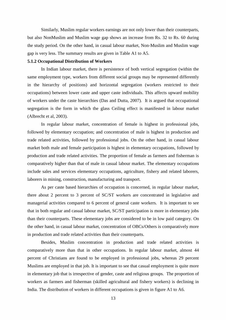
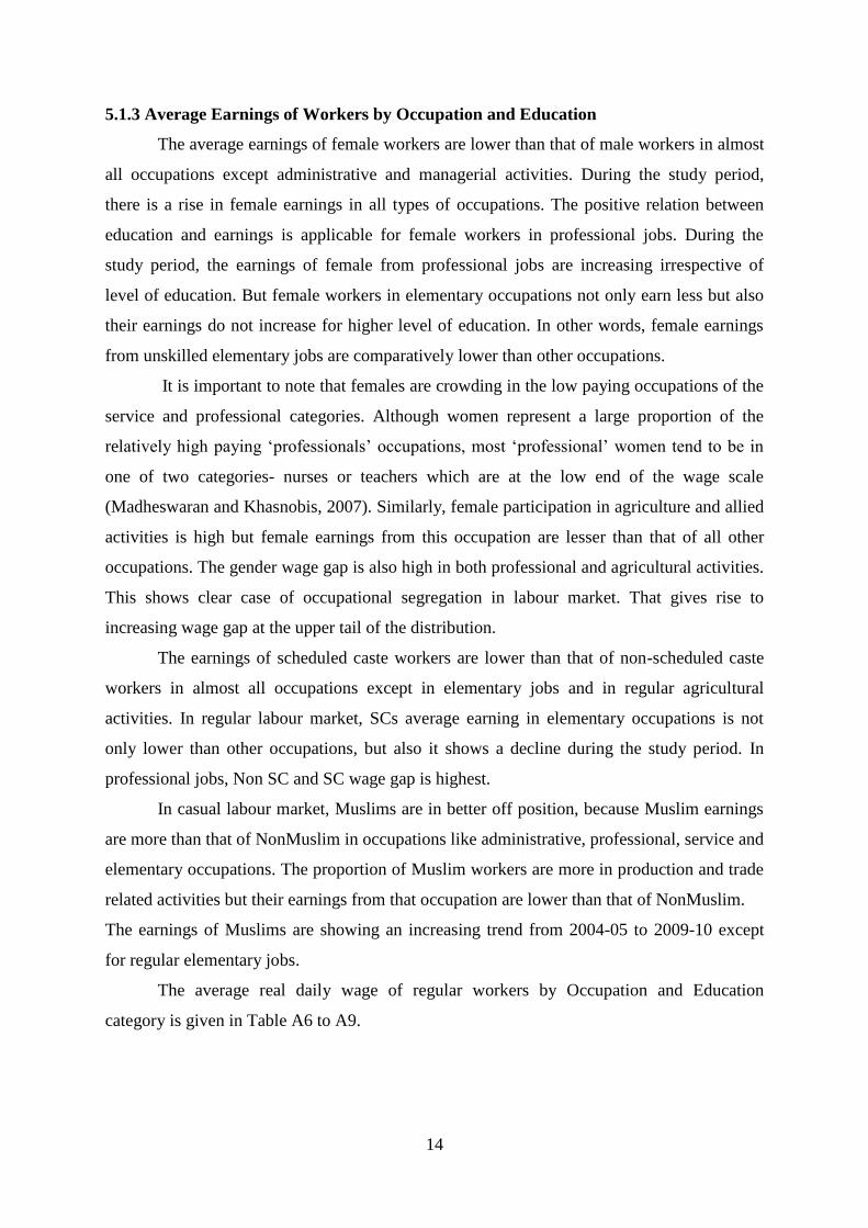
The preliminary evidence of wage gap across the wage distribution is presented in

figure 1 and 2. The gender wage gap among regular workers is high in lower half of the

distribution; this gives prior evidence of „Sticky floor effect‟. During the study period, wage

gap among regular workers shows a decline in lower half of the distribution, but gender wage

gap at the upper half of the distribution remain almost same. For casual workers, gender wage

gap across the wage distribution does not show much variation, but gender wage gap is

narrowing down over the years. This declining gender wage differential is due to higher wage

growth of female workers (Karan and Sakthivel, 2007).

16

We have applied quantile regression method in order to capture, how much of the

observed raw wage gap can be explained by the differences in the returns to various

characteristics. The results reported in Table A14 and A15 make clear that controlling for job

characteristics does not change the sticky floor effect, as we saw in the „uncontrolled‟ log

wage gaps in above figure. In the entire three models, gender wage gap is highest at the 10th

percentile and declines uniformly as one move up the wage distribution to higher percentiles.

In order to establish occupational segregation in labour market, we predict the

estimated wage gap to be higher in Model 2, where occupation dummies are excluded than in

Model 3, where we incorporate occupation dummies. It is only applicable for regular workers

in 10th

to 50th

percentile and for casual workers; we don‟t find any difference in results. There

is occupational segregation among regular workers at low wage quantiles, because the value

of coefficient effect (discrimination) is lower in model 3 than in model 2 (see figure 7).

It is important to keep in mind that quantile regression assumes that returns to the

various characteristics are the same for both men and women across all quantiles. To solve

this, we estimate male and female regression separately.

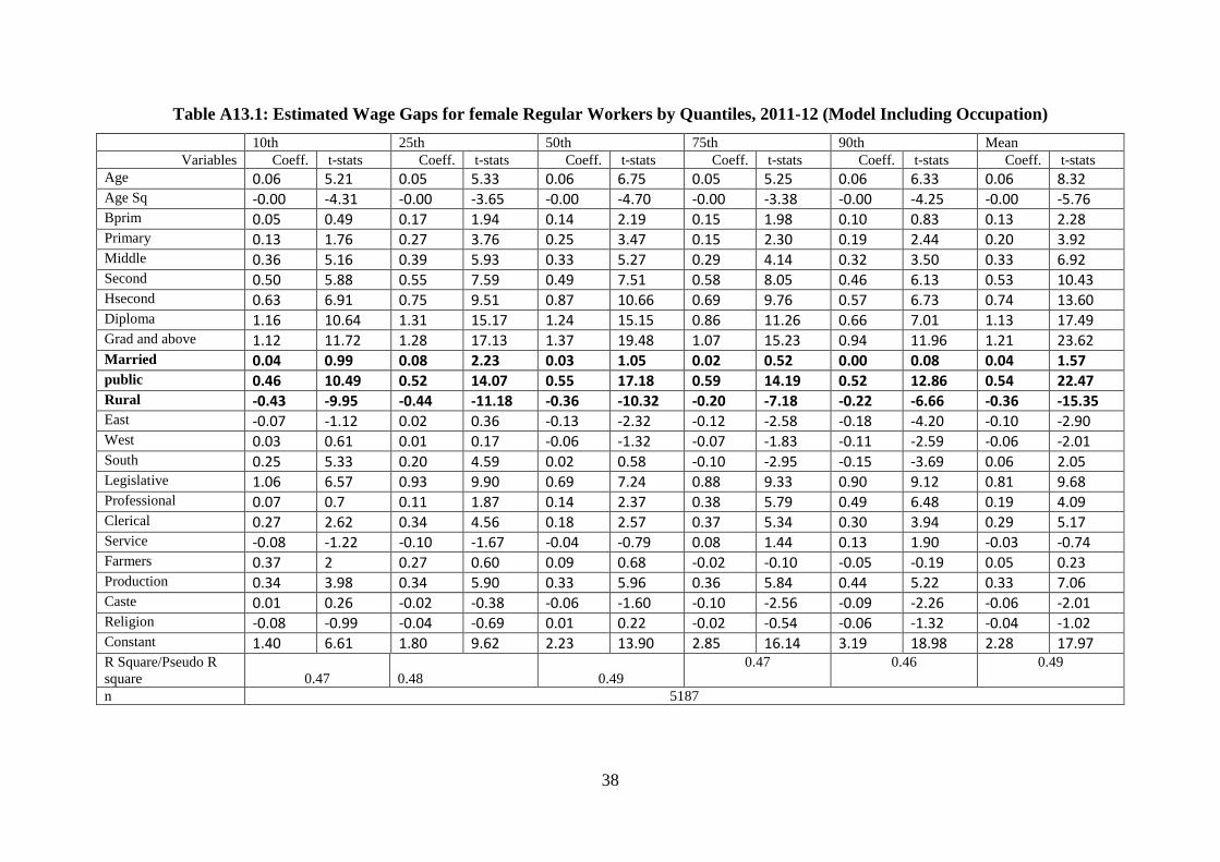
We found that education coefficient is positive and significant for female regular

workers. The regular workers can expect higher earnings for higher levels of education. But

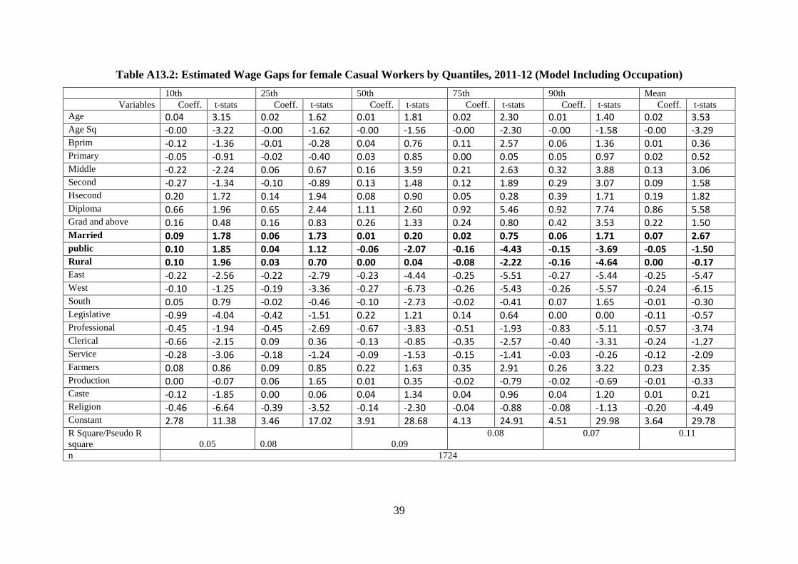
for casual female workers, education coefficient is negative and insignificant in most of the

cases. So there is no association between education and earnings for female casual workers.

We predict that married women are supposed to get lower wages in labour market. But the

estimated coefficient of marital status dummy is positive and insignificant in almost all cases.

On the other hand, rural women are getting lower wages than their counterparts as the

associated coefficients of rural dummy are negative and significant. Particularly, women

working in public sector as regular workers positively affect their earnings. Besides, female

regular workers earnings from skilled occupations like legislators, senior official and

managers are comparatively more than other occupations. However legislative and

managerial activities generally give more premiums to male than to female in regular labour

market. The significant and positive coefficient of clerical occupation dummy implies that the

low paid occupation like clerical jobs pays some premium for the female workers compared

to other occupations. The coefficient of farmer dummy is found statistically significant only

at the upper quantile in casual labour market. The results are reported in Table A13.1 and

A13.2.

The rates of return to education are estimated from the earnings functions of both

male and female; the results are given in Table A25. The rates of return to education at mean

17

are different than other quantiles and across gender. In regular labour market, female rates of

return to education are quite higher than their counterparts irrespective of levels of education.

The female casual workers having below primary and primary education experience negative

returns to education at lower quantiles Q.10 and Q.25, but for their male counterparts it is

positive; and at the upper quantiles, female returns to below primary and primary education

is positive but lesser than their counterparts. Interestingly, at upper quantiles, returns to

female casual workers from higher level of education are more than their counterparts. This

unequal returns to education across the quantiles of wage distribution and between male and

female, give us the incentive to study discrimination in both regular and casual labour market

in India.

It is important to know, whether the gender wage gap is due to endowment difference

or discrimination in labour market. From Table A16, it is clear that more than 90 percent of

mean wage gap between male and female is due to discrimination in labour market. So there

is valuation of personal characteristics unrelated to productivity in India.

The MMM decomposition result in Table A19 and A20 also support the above

findings of large extent of discrimination towards female workers in casual labour market. In

order to empirical test the existence of „Glass Ceiling‟ and „Sticky floor‟ in labour market, the

definition given by Arulampalam et al. (2006) is used. The „Glass ceiling‟ exists, if 90th

percentile wage gap is higher than the estimated wage gaps in other parts of the wage

distribution by at least 2 percentage points. The „Sticky floor‟ is said to exist if 10th

percentile

wage gap is higher than the 25th

percentile wage gap by at least 2 percentage points. The

sticky floor effect in regular labour market is clearly seen in figure 8 as the wage gap is

decreasing throughout the wage distribution. The gender log wage gaps fall from 0.71 at the

10th

percentile to 0.16 at the nineteenth percentile. This finding is consistent with the study

done by Khanna (2012). We found that sticky floor also exists in casual labour market,

because 10th

percentile wage gap is higher than the estimated wage gap at 25th

and 50th

percentile. The sticky floor effect prevails in labour market even after controlling for personal

and job characteristics of workers.

In Figure 10 and 11, we found the wage gap is declining over the years. The decline

in endowment difference has largely contributed to decline in raw wage differentials. The

result reported in Table A19 and A20, shows that the percentage contribution of coefficients

to the raw wage difference has increased from 2004-05 to 2011-12. It implies that the gender

discrimination is widening over the years.

18

The existence of „sticky floor‟ in both regular and casual labour market implies that

women at the lower end of the overall wage distribution experience larger wage gaps

compared to women at the upper end. The study done by Khanna (2012) explains the reason

for the phenomenon of sticky floor effect from different perspectives. The major reason is the

prevalence of statistical discrimination in labour market. According to the theory of statistical

discrimination, employers have relatively sketchy information about the skill endowment of

the individual job applicants but have sound information about the working group. So the

unprejudiced employers give higher wage to those who are from privileged groups, and

unprivileged sections of the society becomes victims of discrimination. Given the higher

probability of dropping out of the women from the labour market, employers discriminate

against women as they enter into the labour market, because they except future career

interruptions.

On the other hand, as women move up the occupation structure and gain job

experience, employers become aware of their reliability and therefore, discriminate less.

Generally, highly educated women are thought to be stable employees. The women working

in high paying jobs are more likely to be employed in managerial or other professional

positions. The scope to discriminate against these workers is lesser given their attributes and

backgrounds. The payment mechanism in high profile jobs would be far more structured and

rigidly defined. Employers would be aware of these possibilities themselves and hence, may

not be able to discriminate a great deal between similarly qualified men and women.

On the contrary, women with no education and working in elementary occupation are

prone to discrimination in labour market. It is easier for the employer to discriminate women

in this case, even if both men and women possess identical labour market characteristics. This

is because; these jobs are informal in nature and outside the jurisdiction of labour laws.

According to the equal remuneration act (1976), there should be equal pay for equal work.

The lack of implementation of the law can be a cause of wage gap at the bottom of the

distribution.

The skilled and unskilled job segregation is also responsible for wider gap at the

bottom of the distribution. The earnings of women in unskilled manual work is very less. The

lack of social security benefits, child care provisions, maternity leave etc. to informal female

workers could be a reason for the higher drop out of female from the labour market; this

make employer to discriminate against them.

19

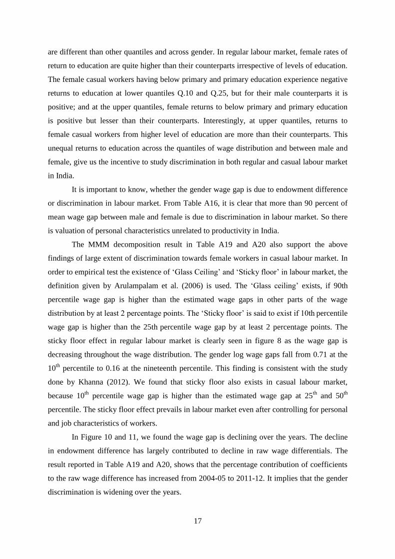
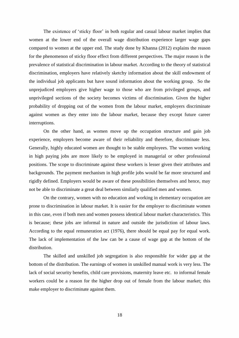
5.2.2 Wage gap by Caste

It is clear that the log wage gap between NonSC and SC regular workers is positive

throughout the distribution. For casual workers, rising wage gap at upper tail of the

distribution gives prediction „Glass Ceiling‟ in labour market. The fig 3 and 4 are plotted

below:

From Table A14, A15, and A17, it is clear that the earnings of SCs are comparatively

lower than Non SC in India. The endowment difference contributes more than 50 percent of

total caste based wage gap in regular labour market. The lower human capital endowment is

the cause of lower earnings of SCs in labour market.

20

The wage gap between SC and NonSC casual workers is increasing throughout the

wage distribution and it is more at the upper tail. Therefore „glass ceiling‟ exists in casual

labour market. We found that there exists occupational segregation in labour market, because

the value of coefficient effect (discrimination) is lower in model 3 than that in other models.

During the study period, the wage gap by caste remains almost same with slight divergence at

both the tails, as shown in figure 12 and 13. It is clear that the percentage contribution of

characteristics (endowment) to raw wage difference has increased over the years, except in

casual worker‟s lower wage distribution. It is important to note that the large endowment

difference implies prevalence of pre-market discriminatory practices in India (see Table A21

and A22).

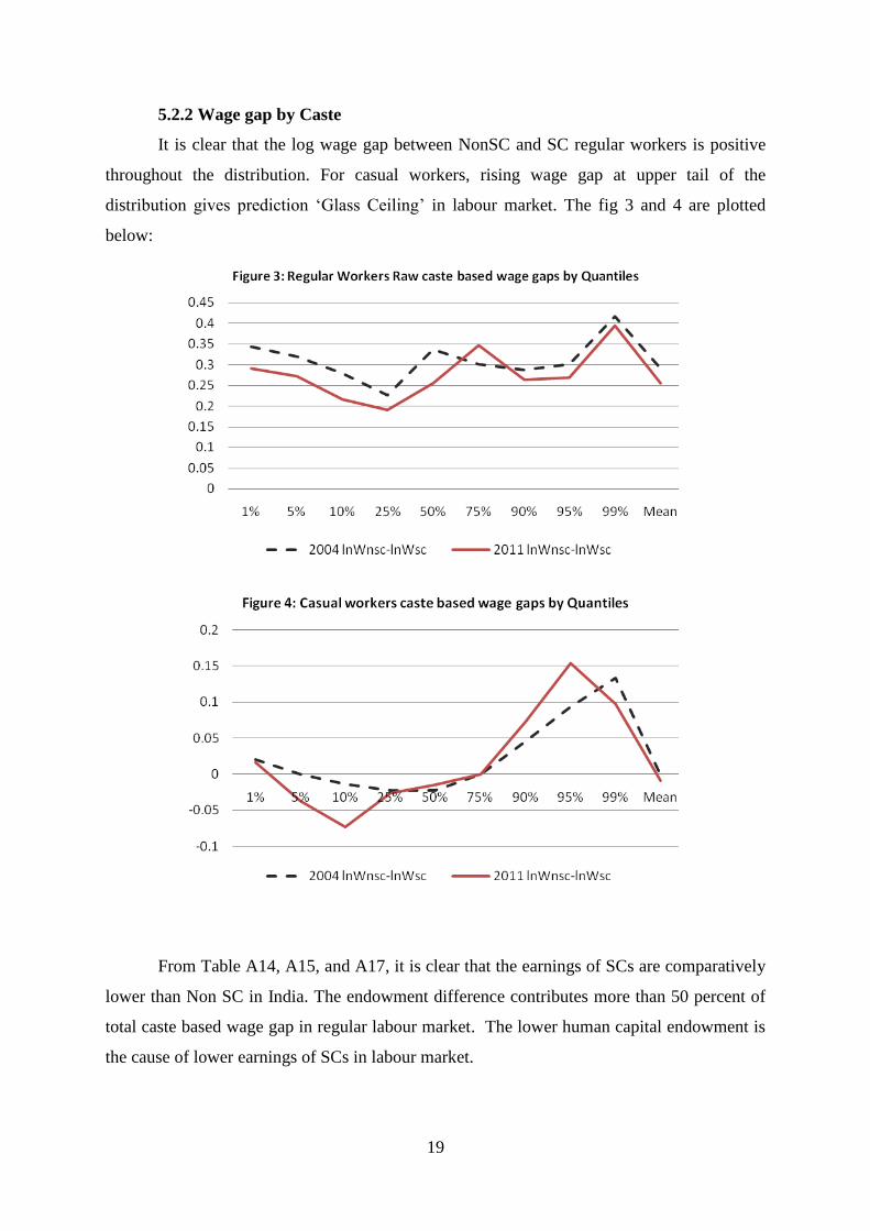
5.2.3 Wage gap by Religion

During the study period, there is an increase in wage gap between Muslim and Non

Muslim regular workers. For regular workers, wage gap by religion is high at upper half of

the distribution; this can be interpreted as the possible existence of „Glass Ceiling effect‟. The

logarithm real daily wage gap by religion is plotted in fig. 5 and 6.

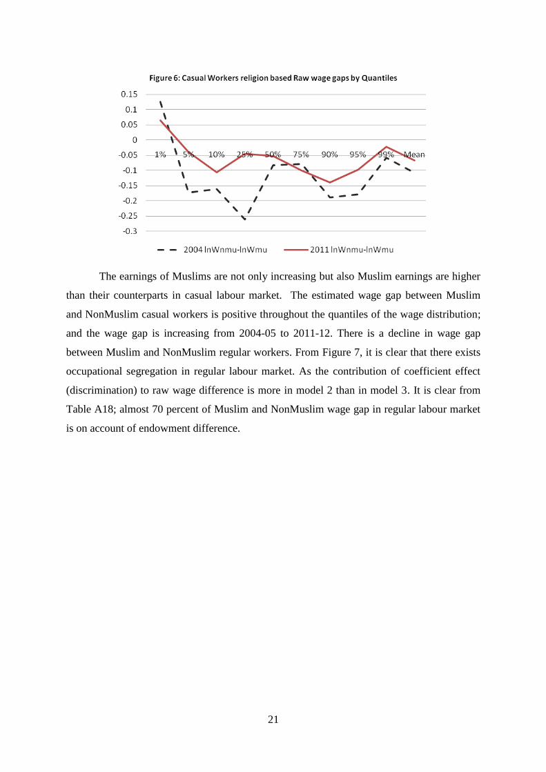
21

The earnings of Muslims are not only increasing but also Muslim earnings are higher

than their counterparts in casual labour market. The estimated wage gap between Muslim

and NonMuslim casual workers is positive throughout the quantiles of the wage distribution;

and the wage gap is increasing from 2004-05 to 2011-12. There is a decline in wage gap

between Muslim and NonMuslim regular workers. From Figure 7, it is clear that there exists

occupational segregation in regular labour market. As the contribution of coefficient effect

(discrimination) to raw wage difference is more in model 2 than in model 3. It is clear from

Table A18; almost 70 percent of Muslim and NonMuslim wage gap in regular labour market

is on account of endowment difference.

22

6 Conclusions

We found existence of „sticky floor‟ in both regular and casual labour market.

Evidence of sticky floor implies that women at the lower end of the overall wage distribution

experience larger wage gaps compared to women at the upper end. It is also evident from our

analysis that in casual labour market, gender discrimination is quite high. In other words,

lower human capital endowment of female is the cause of their lower earnings. The policy

should give importance to female education and skill development, so that they will have

access to high paid occupations. Particularly, discrimination towards educated female is

comparatively lesser than that to uneducated females.

The wage gap between SC and NonSC casual workers is increasing throughout the

wage distribution and it is more at the upper tail. Therefore „glass ceiling‟ exists in casual

labour market. It is due to occupational segregation in labour market. Dalit are still confined

to traditional caste occupations or occupations with low returns. The policy should be in

favor of breaking this hierarchy of occupation in labour market. As far as caste based

discrimination is concerned, we found that the percentage contribution of characteristics

(endowment) to raw wage difference has increased over the years, except in casual worker‟s

lower wage distribution. It is important to note that the large endowment difference implies

prevalence of pre-market discriminatory practices in India. There is a need for continued

government policies aimed at education and skill building for the Scheduled Castes.

The average earnings of Muslims are comparatively lower than that of NonMuslims

in regular labour market. Out of total raw wage gap between Muslim and NonMuslim regular

workers, almost 70 percent is on account of endowment difference. It is proved that there

exists occupational segregation in regular labour market. The policy should aim at increasing

human capital endowment of Muslims so that they can have access to regular jobs.

23

References

1. Agarwal (2013), “Are There Glass-Ceiling and Sticky- Floor Effects in India? An Empirical

Examination”, Oxford Development Studies, vol.41, no.3, pp: 322-342.

2. Albrecht et al. (2003), “Is There a Glass Ceiling in Sweden?", Journal of Labor Economics,

vol. 21, pp: 145-178.

3. Arulampalamn et al. (2006), "Is There a Glass Ceiling over Europe? Exploring the Gender

Pay Gap across the Wage Distribution," Industrial and Labor Relations Review, Cornell

University, ILR School, vol. 60, No. 2, PP: 163-186, January.

4. Azam (2010), “A Distributional Analysis of Public Private Wage Differential in India", IZA

Discussion Paper No. 5132, Institute for the Study of Labour.

5. Azam, M (2009), Changes in Wage Structure in Urban India 1983-2004: a quantile

regression decomposition, IZA DP No. 3963, Institute for the Study of Labour.

6. Chi, Wei & Li, Bo (2008), “Glass Ceiling or Sticky Floor? Examining the Gender Pay Gap

across the Wage Distribution in Urban China, 1987-2004”, Journal of Comparative

Economics, vol. 36, pp: 243-263.

7. Das and Dutta (2007), “Does caste matter for wages in the India labour market?”, Working

Paper, Social Development and Human Development Unit, World Bank, Washington D.C.

8. De la Rica et al. (2005), “Ceiling and Floors: Gender Wage Gaps by Education in Spain”,

IZA Discussion Paper No. 1483, IZA Discussion Papers 1483, Institute for the study of Labor

(IZA).

9. Etienne and Nancy (2010), “Gender wage differentials in the French nonprofit and for-profit

sectors: evidence from quantile regression”, Annals of Economics and Statistics, Issue 99-

100, July/December, pp. 67-90.

10. Juhn and Pierce (1993), “Wage inequality and the rise in return to skill”, The Journal of

Political Economy, vol. 101, pp: 410-442.

11. Khanna (2012), “Gender Wage Discrimination in India: Glass Ceiling or Sticky Floor?”,

working paper No. 214, Center for Development Economics, Delhi school of Economics.

12. Koenker, Roger and Bassett, G. (1978), “Regression Quantiles”, Econometrica, vol. 46,

pp:33-50.

13. Labour Bureau (various years). Indian Labour Statistics, Government of India.

14. Machado and Mata (2005), “Counterfactual Decomposition of Changes in Wage

Distributions Using Quantile Regression”, Journal of Applied Econometrics, vol. 20,pp: 445–

465.

24

15. Madheswaran S. (2010), “Labour market discrimination in India: methodological

developments and empirical evidence”, Indian Journal of Labour Economics, vol. 53, No. 3,

PP: 457-480.

16. Melly, B. (2006), “Estimation of counterfactual distributions using quantile regression”,

University of St. Gallen, Discussion Paper.

17. NSSO (2014), Employment and Unemployment Situation in India, 2011-12, Report No. 554,

National Sample Survey Organization, Department of Statistics and Programme

Implementation, Government of India, New Delhi.

18. Sengupta and Das (2014), “Gender Wage Discrimination across Social and religious groups

in India: estimates with unit level data”, Economic and Political Weekly, vol. XLIX, No. 21,

May.

25

Appendix 1

Table A1: Average Real daily wages by Gender

(With corresponding t-statistics of mean difference)

Male (M) Female (F) F/M Wage Gap (M-F) t-stats

Regular Workers

2004-05 154.23 108.39 0.70 45.84 15.44

2011-12 205.9 159.05 0.77 46.85 10.71

Casual Workers

2004-05 53.39 32.67 0.61 20.72 73.66

2011-12 77.28 58.24 0.75 19.04 29.67

Source: Author‟s calculation based on NSS (2004-05 and 2011-12) data

Table A1.1: Average Real daily wages of Male and Female in regular and casual labour market

across percentiles, 2011-12

Percentiles Male Female Wage Gap(M-F) Male Female Wage Gap(M-F)

Regular Workers Casual Workers

1% 22.86 12.13 10.74 21.94 15.73 6.20

5% 42.99 20.40 22.60 32.90 25.70 7.20

10% 52.08 29.37 22.71 41.12 30.62 10.50

25% 76.21 49.50 26.71 52.44 40.95 11.49

50% 126.51 80.94 45.57 67.99 51.18 16.81

75% 271.11 203.36 67.75 91.94 69.39 22.55

90% 457.28 396.60 60.68 122.75 92.53 30.23

95% 586.83 529.76 57.07 156.42 106.92 49.50

99% 1029.77 931.37 98.41 231.32 180.60 50.72

Source: Author‟s calculation based on NSS (2011-12) data

Table A2: Average Real daily wages of Male and Female in Regular Employment across Social

group (With corresponding t-statistics of mean difference)

Male (M) Female (F) F/M Wage Gap (M-F) t-stats

2004-05

SC 122.55 71.46 0.58 51.09 12.16

ST 133.95 66.37 0.50 67.57 8.15

OBC 130.92 84.14 0.64 46.76 12.28

Others 188.35 154.36 0.82 33.99 5.86

2011-12

SC 167.44 110.56 0.66 56.88 7.78

ST 185.62 114.09 0.61 71.53 4.59

OBC 180.47 137.03 0.76 43.44 7.18

Others 248.14 216.67 0.87 31.46 3.54

Source: Author‟s calculation based on NSS (2004-05 and 2011-12) data

26

Table A3: Average Real daily wages of Male and Female in Regular Employment across

Religious groups (With corresponding t-statistics of mean difference)

Male (M) Female (F) F/M Wage Gap (M-F) t-stats

2004-05

Hindu 157.07 106.38 0.68 50.68 15.36

Muslims 120.81 94.81 0.78 26.11 2.84

Christians 164.31 126.11 0.77 38.20 2.93

Other Minorities 173.43 142.93 0.82 30.50 1.94

2011-12

Hindu 213.92 159.79 0.75 54.13 11.09

Muslims 142.91 129.79 0.91 13.11 1.46

Christians 216.22 176.72 0.82 39.50 1.98

Other Minorities 219.53 195.12 0.89 24.41 0.67

Source: Author‟s calculation based on NSS (2004-05 and 2011-12) data

Table A4: Average Real daily wages by Caste

(With corresponding t-statistics of mean difference)

SC NonSC SC/NonSC

Wage Gap

(NonSC-SC) t-stats

Regular Workers

2004-05 112.19 151.97 0.74 39.78 -14.76

2011-12 150.61 200.28 0.75 49.66 -12.56

Casual Workers

2004-05 46.1 46.88 0.98 0.78 -2.38

2011-12 71.46 72.53 0.99 1.07 -1.6

Source: Author‟s calculation based on NSS (2004-05 and 2011-12) data

Table A5: Average Real daily wages by Religion

(With corresponding t-statistics of mean difference)

Muslim NonMuslim Muslim/NonMuslim

Wage Gap

(NonMuslim-

Muslim) t-stats

Regular Workers

2004-05 115.85 148.13 0.78 32.29 -9.54

2011-12 138.54 198.34 0.70 59.81 -15.77

Casual Workers

2004-05 51.31 46.13 1.11 -5.18 9.85

2011-12 76.76 71.61 1.07 -5.16 5.16

Source: Author‟s calculation based on NSS (2004-05 and 2011-12) data

27

Table A6: Average Real Daily Wage by Occupation, 2004-05

(With corresponding t-statistics of mean difference)

Person Male

(F)

Female

(F)

Wage

Gap

(M-F)

t-stat SC NonSC Wage

Gap

(NonSC-

SC)

t-stat Muslim NonMuslim Wage Gap

(NonMusim-

Muslim)

t-stat

Regular Workers

Administrative

(11-13) 433.03 435.05 393.74 41.31 0.94 292.35 440.08 147.73 3.74 284.57 440.66 156.08 3.01

Professional

(21-34) 227.03 256.82 167.77 89.04 14.1 198.69 230.62 31.93 3.92 187.19 230.73 43.55 4.33

Clerical (41-42) 192.4 192.52 178.99 13.53 1.83 167.92 196.32 28.4 4.33 179.19 193.21 14.01 1.17

Service workers

(51-52) 87.02 102.34 46.53 55.8 22.21 78.12 89.63 11.51 3.7 81.04 87.68 6.64 1.56

Farmers (61-62)

59.42 62.69 45.94 16.75 5.6 60.12 59.22 -0.89 -0.2 79.02 58.63 -20.39

-

2.13

Production (71-83) 102.6 110.93 40.76 70.17 29.74 94.3 104.55 10.26 2.34 80.98 105.4 24.42 6.68

Elementary

(91-93) 105.66 107.94 47.07 60.87 14.1 98.44 107.32 8.88 1.57 103.66 105.96 2.3 0.36

Casual Workers

Administrative

(11-13) 43.55 39.94 27.52 12.41 1.7 38.27 46.82 8.56 1.05 44.51 43.5 -1.004

-

0.11

Professional

(21-34) 66.49 75.91 46.44 29.46 2.92 68.9 58.92 -9.98 -1.11 58.29 67.65 9.35 1.05

Clerical (41-42)

60.05 61.43 47.93 13.5 1.61 49.5 62.59 13.08 1.78 61.12 59.93 -1.19

-

0.11

Service workers

(51-52) 51.33 58.61 37.68 20.93 9.13 46.45 53.24 6.79 2.75 59.07 50.05 -9.02

-

2.63

Farmers (61-62)

39.65 44.95 30.77 14.18 53.1 40.54 39.17 -1.36 -4.53 42.85 39.37 -3.48

-

7.11

Production (71-83) 65.61 70.05 43.83 26.21 29.24 63.56 66.52 2.96 3.12 61.53 66.18 4.66 3.75

Elementary

(91-93) 55.41 58.11 39.78 18.33 19.73 54.35 55.9 1.55 1.72 65.99 53.73 -12.26

-

7.48

Source: Author‟s calculation based on NSS (2004-05) data

28

Table A7: Average Real Daily Wage by Occupation, 2011-12

(With corresponding t-statistics of mean difference)

Person Male

(F)

Female

(F) Wage

Gap

(M-F)

t-stat SC NonSC Wage Gap

(NonSC-

SC)

t-

stat

Muslim NonMuslim Wage Gap

(NonMusim-

Muslim)

t-

stat

Regular Workers

Administrative

(11-13) 479.08 479.98 491.86 -11.88 -0.32 377.91 488.15 110.24 2.01 367.06 486.16 119.09 3.82

Professional

(21-34) 301.68 334.71 240.18 94.53 10.16 252.23 308.44 56.21 5.32 228.73 308.11 79.38 7.11

Clerical (41-42) 223.78 232.33 208.61 23.72 1.98 217.27 224.87 7.59 0.59 203.69 224.95 21.26 1.52

Service workers

(51-52) 129.67 144.44 86.41 58.02 10.65 121.88 131.09 9.22 1.22 104.09 133.32 29.22 5.0

Farmers (61-62)

111.51 122.62 55.39 67.23 5.33 122.29 108.85 -13.44

-

0.71 183.12 107.24 -75.88

-

2.01

Production (71-

83) 135.95 141.61 114.32 27.29 3.49 126.13 138.1 11.97 2.18 108.47 140.88 32.41 6.95

Elementary

(91-93) 87.47 103.33 60.63 42.69 12.52 88.11 87.19 -0.91 -0.2 88.89 87.31 -1.58

-

0.22 Casual Workers

Administrative

(11-13) 95.52 82.81 122.66 -39.86 -0.85 75.68 103.06 27.38 1.15 101.3 94.04 -7.25

-

0.32

Professional

(21-34) 104.52 113.91 77.82 36.09 2.26 78.15 111.26 33.11 2.43 106.16 104.38 -1.77 -0.1

Clerical (41-42) 76.32 81.27 66.55 14.72 1.26 56.77 79.41 22.64 2.82 64.82 78.89 14.07 1.3

Service workers

(51-52) 81.07 87.57 63.81 23.77 4.61 75.76 82.55 6.78 1.0 85.03 80.15 -4.87

-

0.77

Farmers (61-62) 74.34 81.52 66.29 15.22 3.92 68.28 76.53 8.24 1.59 69.95 74.76 4.81 1.1

Production (71-

83) 90.58 94.69 70.66 24.03 12.61 85.37 92.68 7.31 4.55 88.26 91.01 2.74 1.29

Elementary

(91-93) 66.46 71.1 55.07 16.03 23.96 68.09 65.65 -2.43

-

3.48 71.61 65.88 -5.72

-

5.13

Source: Author‟s calculation based on NSS (2011-12) data

29

Table A8: Average Real Daily Wage of Regular Workers by Occupation and Education category, 2004-05

Level of Education Occupation

Administrative Professional clerical service farmer production Elementary

Illiterate &

Non formal

Male 160.51 154.64 116.99 73.89 50.82 85.06 89.11

Female 9.68 25.08 72.01 38.25 42.27 30.70 39.38

Wage Gap 150.83 (2.02) 129.55 (3.56) 44.98 (2.31) 35.63 10.65) 8.54 (2.79) 54.36 (13.55) 49.72 (9.37)

Below primary Male 50.75 80.39 128.66 73.35 51.91 83.04 97.34

Female - 41.69 89.44 37.21 55.27 37.86 58.68

Wage Gap - 38.70 (2.90) 39.22 (2.39) 36.13 (8.49) -3.36 (-0.69) 45.17 (9.48) 38.65 (1.84)

Primary Male 189.36 87.17 139.03 71.59 53.38 84.93 92.38

Female - 72.62 106.61 49.49 47.25 35.98 48.88

Wage Gap - 14.55 (0.67) 32.41 (1.76) 22.09 (3.79) 6.13 (1.37) 48.95 (11.25) 43.49 (3.24)

Middle Male 126.07 118.41 139.59 85.87 87.11 96.67 101.79

Female 38.53 39.09 119.23 46.41 47.93 45.15 56.69

Wage Gap 87.53 (3.99) 79.31 (5.91) 20.35 (1.32) 39.46 (9.03) 39.17 (2.78) 51.52 (11.26) 45.09 (6.37)

Secondary Male 242.41 182.87 174.51 119.99 97.28 126.85 130.83

Female 164.32 106.87 149.82 72.36 59.85 56.83 54.02

Wage Gap 78.09 (0.73) 75.99 (5.58) 24.69 (1.61) 47.63 (4.51) 37.42 (1.35) 70.03 (9.87) 76.80 (7.30)

Higher sec. Male 282.32 208.03 185.73 123.82 94.24 144.77 149.03

Female 349.68 122.43 174.06 94.20 65.22 56.31 -

Wage Gap -67.37 (-0.56) 85.59 (6.03) 11.66 (0.66) 29.61 (1.76) 29.02 (1.45) 88.46 (8.55) -

Diploma Male 364.52 268.21 181.05 157.56 172.81 177.99 212.60

Female 441.04 207.03 204.18 98.41 - 72.86 -

Wage Gap -76.52 (-1.25) 61.18 (4.53) -23.13 (-0.98) 59.14 (1.79) - 105.13 (4.58) -

Grad & above Male 512.34 293.69 247.04 185.46 179.42 175.73 163.38

Female 420.32 206.49 224.85 108.24 - 93.41 121.48

Wage Gap 92.01 (1.86) 87.19 (9.44) 22.18 (1.73) 77.22 (3.79) - 82.32 (1.67) 41.90 (2.83)

Source: Author‟s calculation based on NSS (2004-05) data

Note: Figures in parentheses are t-statistics of mean difference

30

Table A9: Average Real Daily Wage of Regular Workers by Occupation and Education category, 2011-12

Level of Education Occupation

Administrative Professional Clerical Service Farmer Production Elementary

Illiterate &

Non formal

Male 214.10 121.86 96.18 91.48 97.98 104.87 83.81

Female 173.79 134.45 156.18 60.69 42.61 111.63 54.73

Wage Gap 40.31 (0.52) -12.58 (-0.48) -59.99 (-1.06) 30.78 (3.44) 55.36 (3.48) -6.75 (-0.28) 29.08 (5.96)

Below primary Male 93.63 158.30 94.84 83.40 107.16 105.82 106.56

Female 26.86 135.65 192.37 79.63 176.64 113.15 67.37

Wage Gap 66.76 (1.93) 22.64 (0.50) -97.52 (-2.16) 3.76 (0.27) -69.47 (-1.69) -7.33 (-0.29) 39.19 (3.75)

Primary Male 173.65 109.77 161.88 103.51 79.44 116.09 89.45

Female - 105.66 152.43 69.35 80.41 84.58 56.23

Wage Gap - 4.10 (0.15) 9.44 (0.18) 34.14 (3.40) -0.97 31.51 (3.92) 33.21 (6.37)

Middle Male 132.16 175.68 141.75 110.47 139.10 128.39 97.07

Female 754.90 118.50 109.46 67.67 81.83 102.76 63.59

Wage Gap -622.73 (-3.00) 57.18 (2.35) 32.29 (2.14) 42.80 (5.84) 57.26 (2.03) 25.63 (3.36) 33.48 (5.42)

Secondary Male 167.65 223.41 202.05 157.45 133.09 146.46 126.37

Female 300.30 181.04 188.83 115.11 72.67 137.91 77.51

Wage Gap -132.64 (-2.40) 42.37 (1.60) 13.21 (0.55) 42.35 (2.89) 60.42 (2.55) 8.55 (0.58) 48.86 (4.38)

Higher sec. Male 308.46 227.82 228.12 168.18 157.56 157.73 114.75

Female 382.76 181.87 160.91 136.86 189.78 109.68 73.54

Wage Gap -74.29 (-0.91) 45.95 (2.74) 67.21 (3.78) 31.33 (1.61) -32.21 (-1.18) 48.04 (2.83) 41.20 (3.02)

Diploma Male 472.84 325.85 228.73 156.49 114.17 202.77 113.05

Female 395.10 224.82 157.18 68.15 - 181.87 53.40

Wage Gap 77.74 (1.32) 101.02 (5.57) 71.55 (1.54) 88.33 (3.84) - 20.89 (0.40) 59.65 (2.31)

Grad & above Male 565.63 386.53 270.59 218.53 219.90 254.80 182.85

Female 527.86 287.02 252.89 174.18 177.73 184.07 164.07

Wage Gap 37.76(0.91) 99.50 (7.46) 17.69 (0.93) 44.34 (1.42) 42.17 (0.47) 70.73 (2.81) 18.77 (0.20)

Source: Author‟s calculation based on NSS (2011-12) data

Note: Figures in parentheses are t-statistics of mean difference

31

32

33

34

Appendix 2

Table A10: Descriptive Statistics of Main Variables used in Estimation

Variables Description of Variables Regular Casual

2004-05 2011-12 2004-05 2011-12

Mean Stand.

dev.

Mean Stand.

dev.

Mean Stand.

Dev.

Mean Stand.

Dev.

Real Wage Real daily wage(in rupees) 153.97 145.61 210.48 200.85 51.91 31.03 80.93 45.91

Lnreal Wage Logarithm of real daily wage (in Rupees) 4.62 0.95 4.95 0.93 3.80 0.54 4.26 0.52

Age 15 to 65 Years of age 36.41 11.33 37.08 11.14 33.80 11.92 35.94 12.13

Age Sq Age Square in years 1453.85 858.78 1499.07 865.17 1284.42 886.84 1438.81 943.18

Bprim If the worker has completed below primary education =1;0

otherwise 0.05 0.22 0.05 0.22 0.11 0.32 0.14 0.35

Primary If the worker has completed primary education =1;0 otherwise 0.10 0.31 0.08 0.27 0.16 0.36 0.17 0.38

Middle If the worker has completed middle school =1;0 otherwise 0.17 0.37 0.14 0.35 0.15 0.36 0.18 0.38

Second If the worker has completed secondary school=1;0 otherwise 0.16 0.36 0.16 0.36 0.05 0.21 0.09 0.29

Hsecond If the worker has completed higher secondary school=1;0

otherwise 0.11 0.31 0.13 0.34 0.01 0.12 0.03 0.18

Diploma If the worker has completed diploma =1;0 otherwise 0.06 0.24 0.05 0.21 0.00 0.06 0.01 0.07

Grad and

above

If the worker has completed graduate and above degree=1;0

otherwise 0.23 0.42 0.31 0.46 0.00 0.06 0.01 0.10

Married If the individual is married=1;0 otherwise 0.74 0.44 0.75 0.44 0.71 0.45 0.71 0.45

public If the worker is working in public sector=1;0 otherwise 0.51 0.50 0.56 0.50 0.06 0.24 0.10 0.30

Rural If the worker is working in rural areas=1;0 otherwise 0.40 0.49 0.39 0.49 0.77 0.42 0.75 0.44

East If the individual is working in east=1; 0 otherwise 0.13 0.33 0.14 0.34 0.19 0.39 0.18 0.39

West If the individual is working in west=1; 0 otherwise 0.26 0.44 0.24 0.43 0.23 0.42 0.19 0.39

South If the individual is working in south=1; 0 otherwise 0.31 0.46 0.31 0.46 0.36 0.48 0.35 0.48

Legislative If the individual occupation is Legislative=1; 0 otherwise 0.03 0.16 0.04 0.20 0.00 0.04 0.00 0.04

Professional If the individual occupation is professional=1; 0 otherwise 0.23 0.42 0.31 0.46 0.00 0.05 0.01 0.08

Clerical If the individual occupation is clerical=1; 0 otherwise 0.18 0.39 0.10 0.31 0.00 0.06 0.00 0.04

Service If the individual occupation is service =1; 0 otherwise 0.23 0.42 0.16 0.37 0.04 0.20 0.02 0.15

Farmers If the individual occupation is agriculture=1; 0 otherwise 0.04 0.19 0.01 0.09 0.55 0.50 0.03 0.18

Production If the individual occupation is production=1; 0 otherwise 0.21 0.41 0.25 0.43 0.26 0.44 0.30 0.46

Gender If the worker is Male=1; 0 otherwise 0.80 0.40 0.77 0.42 0.71 0.45 0.75 0.43

Caste If the worker belong to Scheduled Caste=1; 0 otherwise 0.17 0.38 0.17 0.37 0.32 0.46 0.29 0.46

Religion If the worker belong to Muslim community=1; 0 otherwise 0.11 0.311106 0.12 0.33 0.11 0.32 0.14 0.34

35

Table A11: Estimated Wage Gaps for Regular Workers by Quantiles, 2011-12 (Model with Basic Control Variable)

10th 25th 50th 75th 90th Mean

Variables Coeff. t-stats Coeff. t-stats Coeff. t-stats Coeff. t-stats Coeff. t-stats Coeff. t-stats

Age 0.07 14.45 0.07 17.94 0.06 18.57 0.07 23.28 0.07 19.2 0.07 26.05 Age Sq -0.00 -10.99 -0.00 -11.83 -0.00 -9.57 -0.00 -13.15 -0.00 -11.79 -0.00 -16.16 Bprim 0.14 3.23 0.15 5.22 0.12 4.28 0.09 2.83 0.07 1.75 0.13 5.75 Primary 0.18 4.29 0.20 7.75 0.21 8.85 0.20 7.61 0.11 3.27 0.20 9.59 Middle 0.36 9.55 0.33 15.43 0.34 15.91 0.33 13.1 0.24 7.64 0.35 18.94 Second 0.54 13.95 0.52 23.97 0.58 26.39 0.58 24.1 0.49 15.7 0.58 31.27 Hsecond 0.62 15.32 0.69 28.27 0.85 35.13 0.82 34.36 0.67 21.36 0.78 40.59 Diploma 0.99 18.24 1.09 37.12 1.14 39.99 1.05 39.19 0.87 25.52 1.08 45.96 Grad and above 1.01 25.15 1.26 55.02 1.36 68.37 1.25 56.11 1.12 37.62 1.25 73.01 Gender 0.56 27.17 0.49 31.06 0.33 21.8 0.16 12.77 0.08 4.74 0.32 28.93 Caste -0.06 -2.72 -0.05 -3.25 -0.05 -3.39 -0.05 -3.63 -0.05 -3.25 -0.05 -4.59 Religion 0.01 0.36 0.06 2.85 0.09 5.46 0.05 3.87 0.05 2.47 0.06 4.51 Constant 1.41 14.43 1.84 25.59 2.41 38.82 2.85 49.06 3.31 44.01 2.30 45.40 R Square/Pseudo R Square

0.35 0.38 0.39 0.38 0.37 0.39

n 30312

Source: Author‟s Calculation

36

Table A12: Estimated Wage Gaps for Regular Workers by Quantiles, 2011-12 (Model Excluding Occupation)

10th 25th 50th 75th 90th Mean

Variables Coeff. t-stats Coeff. t-stats Coeff. t-stats Coeff. t-stats Coeff. t-stats Coeff. t-stats

Age 0.05 9.66 0.04 10.48 0.04 10.59 0.04 13.45 0.04 10.39 0.04 15.81

Age Sq -0.00 -7.21 -0.00 -6.46 -0.00 -5.19 -0.00 -7.29 -0.00 -5.71 -0.00 -9.58

Bprim 0.23 5.98 0.21 6.47 0.18 6.13 0.07 2.83 0.06 1.7 0.16 6.8

Primary 0.21 5.8 0.22 7.65 0.26 9.32 0.17 7.26 0.14 4.58 0.22 10.96

Middle 0.30 9.29 0.31 11.98 0.30 12.56 0.26 11.6 0.25 8.73 0.31 17.28

Second 0.44 12.93 0.46 17.12 0.46 19.04 0.42 19.29 0.41 15.66 0.47 26.3

Hsecond 0.52 14.79 0.59 20.66 0.63 25.75 0.57 25.24 0.56 20.88 0.62 33.38

Diploma 0.82 18.82 0.91 26.94 0.91 30.56 0.82 32.04 0.77 25.48 0.90 38.37

Grad and above 0.89 27.16 1.06 40.19 1.04 43.94 0.98 44.41 1.01 37.32 1.04 62.24

Married 0.18 8.61 0.15 8.23 0.13 8.6 0.08 5.63 0.06 3.32 0.12 10.55

public 0.42 28.15 0.52 41.43 0.61 49.06 0.58 45.66 0.52 32.99 0.54 60.28

Rural -0.27 -17 -0.21 -17.09 -0.15 -15.33 -0.16 -17.17 -0.17 -13.8 -0.21 -24.74

East -0.11 -4.13 -0.14 -7.38 -0.15 -10.23 -0.12 -8.91 -0.11 -6.66 -0.13 -10.44

West -0.03 -1.33 -0.12 -7.56 -0.13 -9.71 -0.11 -9.31 -0.08 -5.16 -0.11 -10.57

South 0.10 5.24 -0.02 -1.24 -0.07 -5.95 -0.07 -6.31 -0.05 -3.28 -0.04 -3.55

Gender 0.65 33.72 0.57 32.86 0.37 21.27 0.23 17.19 0.18 10.72 0.40 37.88

Caste -0.07 -3.48 -0.07 -4.06 -0.07 -4.72 -0.06 -4.58 -0.07 -4.36 -0.07 -5.9

Religion -0.01 -0.31 0.04 2.49 0.05 3.64 0.02 1.86 0.02 0.94 0.03 2.65

Constant 1.68 18.02 2.12 27.19 2.80 42.63 3.30 53.93 3.67 46.87 2.67 51.05

R Square/Pseudo R square

0.45 0.47 0.48

0.47

0.47

0.48

n 27509

Source: Author‟s Calculation

37

Table A13: Estimated Wage Gaps for Regular Workers by Quantiles, 2011-12 (Model Including Occupation)

10th 25th 50th 75th 90th Mean

Variables Coeff. t-stats Coeff. t-stats Coeff. t-stats Coeff. t-stats Coeff. t-stats Coeff. t-stats

Age 0.05 10.77 0.04 9.44 0.04 11.3 0.04 12.67 0.05 11.27 0.04 16.24 Age Sq -0.00 -8.1 -0.00 -5.68 -0.00 -6.13 -0.00 -7.3 -0.00 -6.93 -0.00 -10.14 Bprim 0.19 4.53 0.14 4.31 0.11 4.28 0.05 2.09 0.08 2.33 0.13 5.44 Primary 0.19 5.32 0.16 5.38 0.17 6.74 0.14 6.51 0.14 4.51 0.18 8.79 Middle 0.26 8.55 0.23 8.36 0.23 10.12 0.21 9.86 0.21 8.29 0.24 13.45 Second 0.37 12.65 0.35 12.38 0.34 15.01 0.34 16.19 0.35 14.07 0.37 20.43 Hsecond 0.41 12.05 0.44 14.21 0.46 18.75 0.44 19.48 0.42 15.96 0.47 24.25 Diploma 0.70 15.69 0.71 20.11 0.64 22.1 0.58 22.61 0.52 15 0.68 28.16 Grad and above 0.75 21.86 0.83 27.68 0.75 30.59 0.70 31.17 0.71 25.4 0.80 41.62 Married 0.16 8.22 0.13 7.35 0.11 7.34 0.06 4.66 0.04 2.5 0.10 8.98 public 0.43 27.98 0.52 40.52 0.60 48.25 0.58 47.48 0.51 33.72 0.53 59.99 Rural -0.29 -18.28 -0.22 -18.06 -0.17 -16.32 -0.16 -18.74 -0.19 -16.69 -0.22 -26.61 East -0.11 -4.71 -0.15 -7.82 -0.15 -9.59 -0.12 -9.85 -0.13 -7.81 -0.14 -11.39 West -0.05 -2.4 -0.12 -7.07 -0.12 -9.64 -0.11 -9.25 -0.10 -6.32 -0.11 -10.78 South 0.08 4.01 -0.01 -0.86 -0.08 -6.38 -0.07 -6.46 -0.07 -4.34 -0.04 -4.31 Legislative 0.59 6.18 0.72 18.86 0.77 27.49 0.78 28.11 0.74 21.97 0.70 29 Professional 0.32 11.86 0.42 15.57 0.51 23.94 0.48 25.83 0.48 20.69 0.42 25.72 Clerical 0.30 9.7 0.34 11.89 0.36 15.89 0.29 14.82 0.25 10.11 0.31 16.88 Service 0.14 5.17 0.17 6.73 0.20 10.37 0.17 9.5 0.14 6.28 0.15 9.63 Farmers 0.15 1.83 0.12 0.86 0.22 3.15 0.24 5.15 0.16 3.21 0.18 3.59 Production 0.33 14.53 0.33 14.53 0.30 17.73 0.26 16.59 0.22 10.9 0.29 19.91 Gender 0.63 29.99 0.56 29.97 0.36 22.66 0.25 18.99 0.19 11.27 0.40 37.36 Caste -0.03 -1.61 -0.05 -3.36 -0.04 -3.25 -0.04 -3.7 -0.06 -3.91 -0.04 -3.97 Religion -0.01 -0.35 0.03 1.73 0.03 2.02 0.01 1.16 0.00 -0.04 0.02 1.59 Constant 1.48 15.98 2.03 24.41 2.66 40.38 3.18 51.19 3.53 45.77 2.55 49.29 R Square/Pseudo R

square

0.47 0.49 0.50

0.49 0.49 0.50

n 27438

Source: Author‟s Calculation

38

Table A13.1: Estimated Wage Gaps for female Regular Workers by Quantiles, 2011-12 (Model Including Occupation)

10th 25th 50th 75th 90th Mean

Variables Coeff. t-stats Coeff. t-stats Coeff. t-stats Coeff. t-stats Coeff. t-stats Coeff. t-stats

Age 0.06 5.21 0.05 5.33 0.06 6.75 0.05 5.25 0.06 6.33 0.06 8.32 Age Sq -0.00 -4.31 -0.00 -3.65 -0.00 -4.70 -0.00 -3.38 -0.00 -4.25 -0.00 -5.76 Bprim 0.05 0.49 0.17 1.94 0.14 2.19 0.15 1.98 0.10 0.83 0.13 2.28 Primary 0.13 1.76 0.27 3.76 0.25 3.47 0.15 2.30 0.19 2.44 0.20 3.92 Middle 0.36 5.16 0.39 5.93 0.33 5.27 0.29 4.14 0.32 3.50 0.33 6.92 Second 0.50 5.88 0.55 7.59 0.49 7.51 0.58 8.05 0.46 6.13 0.53 10.43 Hsecond 0.63 6.91 0.75 9.51 0.87 10.66 0.69 9.76 0.57 6.73 0.74 13.60 Diploma 1.16 10.64 1.31 15.17 1.24 15.15 0.86 11.26 0.66 7.01 1.13 17.49 Grad and above 1.12 11.72 1.28 17.13 1.37 19.48 1.07 15.23 0.94 11.96 1.21 23.62 Married 0.04 0.99 0.08 2.23 0.03 1.05 0.02 0.52 0.00 0.08 0.04 1.57 public 0.46 10.49 0.52 14.07 0.55 17.18 0.59 14.19 0.52 12.86 0.54 22.47 Rural -0.43 -9.95 -0.44 -11.18 -0.36 -10.32 -0.20 -7.18 -0.22 -6.66 -0.36 -15.35 East -0.07 -1.12 0.02 0.36 -0.13 -2.32 -0.12 -2.58 -0.18 -4.20 -0.10 -2.90 West 0.03 0.61 0.01 0.17 -0.06 -1.32 -0.07 -1.83 -0.11 -2.59 -0.06 -2.01 South 0.25 5.33 0.20 4.59 0.02 0.58 -0.10 -2.95 -0.15 -3.69 0.06 2.05 Legislative 1.06 6.57 0.93 9.90 0.69 7.24 0.88 9.33 0.90 9.12 0.81 9.68 Professional 0.07 0.7 0.11 1.87 0.14 2.37 0.38 5.79 0.49 6.48 0.19 4.09 Clerical 0.27 2.62 0.34 4.56 0.18 2.57 0.37 5.34 0.30 3.94 0.29 5.17 Service -0.08 -1.22 -0.10 -1.67 -0.04 -0.79 0.08 1.44 0.13 1.90 -0.03 -0.74 Farmers 0.37 2 0.27 0.60 0.09 0.68 -0.02 -0.10 -0.05 -0.19 0.05 0.23 Production 0.34 3.98 0.34 5.90 0.33 5.96 0.36 5.84 0.44 5.22 0.33 7.06 Caste 0.01 0.26 -0.02 -0.38 -0.06 -1.60 -0.10 -2.56 -0.09 -2.26 -0.06 -2.01 Religion -0.08 -0.99 -0.04 -0.69 0.01 0.22 -0.02 -0.54 -0.06 -1.32 -0.04 -1.02 Constant 1.40 6.61 1.80 9.62 2.23 13.90 2.85 16.14 3.19 18.98 2.28 17.97 R Square/Pseudo R

square

0.47 0.48 0.49

0.47 0.46 0.49

n 5187

39

Table A13.2: Estimated Wage Gaps for female Casual Workers by Quantiles, 2011-12 (Model Including Occupation)

10th 25th 50th 75th 90th Mean

Variables Coeff. t-stats Coeff. t-stats Coeff. t-stats Coeff. t-stats Coeff. t-stats Coeff. t-stats

Age 0.04 3.15 0.02 1.62 0.01 1.81 0.02 2.30 0.01 1.40 0.02 3.53 Age Sq -0.00 -3.22 -0.00 -1.62 -0.00 -1.56 -0.00 -2.30 -0.00 -1.58 -0.00 -3.29 Bprim -0.12 -1.36 -0.01 -0.28 0.04 0.76 0.11 2.57 0.06 1.36 0.01 0.36 Primary -0.05 -0.91 -0.02 -0.40 0.03 0.85 0.00 0.05 0.05 0.97 0.02 0.52 Middle -0.22 -2.24 0.06 0.67 0.16 3.59 0.21 2.63 0.32 3.88 0.13 3.06 Second -0.27 -1.34 -0.10 -0.89 0.13 1.48 0.12 1.89 0.29 3.07 0.09 1.58 Hsecond 0.20 1.72 0.14 1.94 0.08 0.90 0.05 0.28 0.39 1.71 0.19 1.82 Diploma 0.66 1.96 0.65 2.44 1.11 2.60 0.92 5.46 0.92 7.74 0.86 5.58 Grad and above 0.16 0.48 0.16 0.83 0.26 1.33 0.24 0.80 0.42 3.53 0.22 1.50 Married 0.09 1.78 0.06 1.73 0.01 0.20 0.02 0.75 0.06 1.71 0.07 2.67 public 0.10 1.85 0.04 1.12 -0.06 -2.07 -0.16 -4.43 -0.15 -3.69 -0.05 -1.50 Rural 0.10 1.96 0.03 0.70 0.00 0.04 -0.08 -2.22 -0.16 -4.64 0.00 -0.17 East -0.22 -2.56 -0.22 -2.79 -0.23 -4.44 -0.25 -5.51 -0.27 -5.44 -0.25 -5.47 West -0.10 -1.25 -0.19 -3.36 -0.27 -6.73 -0.26 -5.43 -0.26 -5.57 -0.24 -6.15 South 0.05 0.79 -0.02 -0.46 -0.10 -2.73 -0.02 -0.41 0.07 1.65 -0.01 -0.30 Legislative -0.99 -4.04 -0.42 -1.51 0.22 1.21 0.14 0.64 0.00 0.00 -0.11 -0.57 Professional -0.45 -1.94 -0.45 -2.69 -0.67 -3.83 -0.51 -1.93 -0.83 -5.11 -0.57 -3.74 Clerical -0.66 -2.15 0.09 0.36 -0.13 -0.85 -0.35 -2.57 -0.40 -3.31 -0.24 -1.27 Service -0.28 -3.06 -0.18 -1.24 -0.09 -1.53 -0.15 -1.41 -0.03 -0.26 -0.12 -2.09 Farmers 0.08 0.86 0.09 0.85 0.22 1.63 0.35 2.91 0.26 3.22 0.23 2.35 Production 0.00 -0.07 0.06 1.65 0.01 0.35 -0.02 -0.79 -0.02 -0.69 -0.01 -0.33 Caste -0.12 -1.85 0.00 0.06 0.04 1.34 0.04 0.96 0.04 1.20 0.01 0.21 Religion -0.46 -6.64 -0.39 -3.52 -0.14 -2.30 -0.04 -0.88 -0.08 -1.13 -0.20 -4.49 Constant 2.78 11.38 3.46 17.02 3.91 28.68 4.13 24.91 4.51 29.98 3.64 29.78 R Square/Pseudo R

square

0.05 0.08 0.09

0.08 0.07 0.11

n 1724

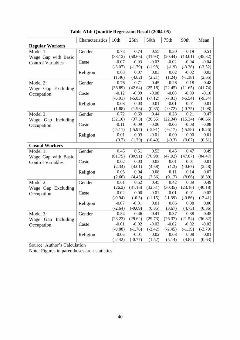
40

Table A14: Quantile Regression Result (2004-05)

Characteristics 10th 25th 50th 75th 90th Mean

Regular Workers

Model 1:

Wage Gap with Basic

Control Variables

Gender 0.73

(38.12)

0.74

(50.65)

0.55

(31.93)

0.30

(20.44)

0.19

(13.01)

0.51

(45.32)

Caste -0.07

(-3.07)

-0.03

(-1.79)

-0.03

(-1.98)

-0.02

(-1.9)

-0.04

(-3.38)

-0.04

(-3.52)

Religion 0.03

(1.46)

0.07

(4.02)

0.03

(2.21)

0.02

(1.24)

-0.02

(-1.38)

0.03

(2.65)

Model 2:

Wage Gap Excluding

Occupation

Gender 0.76

(36.89)

0.71

(42.64)

0.45

(25.18)

0.26

(22.45)

0.18

(11.65)

0.48

(41.74)

Caste -0.12

(-6.01)

-0.09

(-5.83)

-0.08

(-7.12)

-0.08

(-7.81)

-0.09

(-6.54)

-0.10

(-9.34)

Religion 0.03

(1.88)

0.03

(1.93)

0.01

(0.85)

-0.01

(-0.72)

-0.01

(-0.75)

0.01

(1.08)

Model 3:

Wage Gap Including

Occupation

Gender 0.72

(32.16)

0.69

(37.3)

0.44

(26.35)

0.28

(22.34)

0.21

(15.34)

0.47

(40.66)

Caste -0.11

(-5.11)

-0.09

(-5.97)

-0.06

(-5.91)

-0.06

(-6.17)

-0.08

(-5.58)

-0.08

(-8.26)

Religion 0.01

(0.7)

0.03

(1.79)

-0.01

(-0.49)

0.00

(-0.3)

0.00

(0.07)

0.01

(0.51)

Casual Workers

Model 1:

Wage Gap with Basic

Control Variables

Gender 0.45

(61.75)

0.51

(80.91)

0.53

(70.98)

0.45

(47.92)

0.47

(47.87)

0.49

(84.47)

Caste 0.02

(2.34)

0.03

(4.01)

0.03

(4.58)

0.01

(1.3)

-0.01

(-0.67)

0.01

(2.48)

Religion 0.05

(2.66)

0.04

(4.46)

0.08

(7.36)

0.11

(9.17)

0.14

(8.66)

0.07

(8.39)

Model 2:

Wage Gap Excluding

Occupation

Gender 0.61

(26.2)

0.52

(31.16)

0.45

(32.31)

0.42

(30.35)

0.39

(23.16)

0.49

(40.18)

Caste -0.02

(-0.94)

0.00

(-0.3)

-0.01

(-1.15)

-0.01

(-1.39)

-0.01

(-0.86)

-0.02

(-2.41)

Religion -0.07

(-2.64)

-0.01

(-0.69)

0.01

(0.85)

0.06

(3.67)

0.08

(4.73)

0.00

(0.36)

Model 3:

Wage Gap Including

Occupation

Gender 0.54

(23.23)

0.46

(29.62)

0.41

(29.73)

0.37

(26.37)

0.38

(21.54)

0.45

(36.82)

Caste -0.01

(-0.88)

-0.02

(-1.76)

-0.02

(-2.42)

-0.02

(-2.45)

-0.02

(-1.19)

-0.02

(-2.79)

Religion -0.06

(-2.42)

-0.01

(-0.77)

0.02

(1.52)

0.08

(5.14)

0.08

(4.82)

0.01

(0.63)

Source: Author‟s Calculation

Note: Figures in parentheses are t-statistics

41

Table A15: Quantile Regression Result (2011-12)

Characteristics 10th 25th 50th 75th 90th Mean

Regular Workers

Model 1:

Wage Gap with Basic

Control Variables

Gender 0.56

(27.17)

0.49

(31.06)

0.33

(21.8)

0.16

(12.77)

0.08

(4.74)

0.32

(28.93)

Caste -0.06

(-2.72)

-0.05

(-3.25)

-0.05

(-3.39)

-0.05

(-3.63)

-0.05

(-3.25)

-0.05

(-4.59)

Religion 0.01

(0.36)

0.06

(2.85)

0.09

(5.46)

0.05

(3.87)

0.05

(2.47)

0.06

(4.51)

Model 2:

Wage Gap Excluding

Occupation

Gender 0.65

(33.72)

0.57

(32.86)

0.37

(21.27)

0.23

(17.19)

0.18

(10.72)

0.40

(37.88)

Caste -0.07

(-3.48)

-0.07

(-4.06)

-0.07

(-4.72)

-0.06

(-4.58)

-0.07

(-4.36)

-0.07

(-5.9)

Religion -0.01

(-0.31)

0.04

(2.49)

0.05

(3.64)

0.02

1.86)(

0.02

(0.94)

0.03

(2.65)

Model 3:

Wage Gap Including

Occupation

Gender 0.63

(29.99)

0.56

(29.97)

0.36

(22.66)

0.25

(18.99)

0.19

(11.27)

0.40

(37.36)

Caste -0.03

(-1.61)

-0.05

(-3.36)

-0.04

(-3.25)

-0.04

(-3.7)

-0.06

(-3.91)

-0.04

(-3.97)

Religion -0.01

(-0.35)

0.03

(1.73)

0.03

(2.02)

0.01

(1.16)

0.00

(-0.04)

0.02

(1.59)

Casual Workers

Model 1:

Wage Gap with Basic

Control Variables

Gender 0.35

(27.1)

0.27

(28.18)

0.32

(39.02)

0.28

(30.65)

0.25

(16.93)

0.28

(38.78)

Caste 0.06

(5.0)

0.07

(7.69)

0.04

(5.32)

0.02

(2.73)

-0.04

(-3.18)

0.02

(3.23)

Religion 0.10

(5.94)

0.13

(11.53)

0.11

(10.82)

0.14

(11.01)

0.14

(7.97)

0.12

(12.33)

Model 2:

Wage Gap Excluding

Occupation

Gender 0.50

(12.53)

0.41

(23.82)

0.36

(21.51)

0.33

(21.8)

0.24

(10.93)

0.40

(28.11)

Caste 0.02

(0.91)

0.00

(0.32)

0.01

(0.82)

-0.01

(-1.58)

-0.01

(-0.88)

-0.01

(-1.03)

Religion 0.00

(-0.13)

0.01

(0.91)

0.04

(3.3)

0.08

(6.72)

0.10

(5.74)

0.04

(3.44)

Model 3:

Wage Gap Including

Occupation

Gender 0.49

(13.04)

0.42

(21.34)

0.36

(21.57)

0.33

(20.82)

0.24

(10.13)

0.39

(27.31)

Caste -0.01

(-0.36)

0.00

(-0.13)

0.01

(1.03)

-0.01

(-0.7)

-0.01

(-0.76)

-0.01

(-1.09)

Religion -0.02

(-1.06)

0.01

(0.93)

0.05

(4.23)

0.10

(8.05)

0.11

(6.39)

0.04

(3.92)

Source: Author‟s Calculation

Note: Figures in parentheses are t-statistics

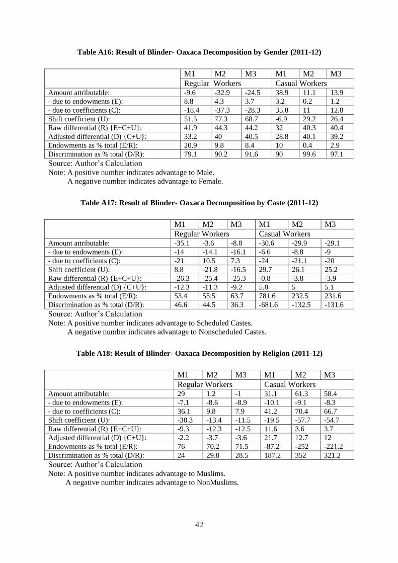
42

Table A16: Result of Blinder- Oaxaca Decomposition by Gender (2011-12)

M1 M2 M3 M1 M2 M3

Regular Workers Casual Workers Amount attributable: -9.6 -32.9 -24.5 38.9 11.1 13.9

- due to endowments (E): 8.8 4.3 3.7 3.2 0.2 1.2

- due to coefficients (C): -18.4 -37.3 -28.3 35.8 11 12.8

Shift coefficient (U): 51.5 77.3 68.7 -6.9 29.2 26.4

Raw differential (R) {E+C+U}: 41.9 44.3 44.2 32 40.3 40.4

Adjusted differential (D) {C+U}: 33.2 40 40.5 28.8 40.1 39.2

Endowments as % total (E/R): 20.9 9.8 8.4 10 0.4 2.9

Discrimination as % total (D/R): 79.1 90.2 91.6 90 99.6 97.1

Source: Author‟s Calculation Note: A positive number indicates advantage to Male.

A negative number indicates advantage to Female.

Table A17: Result of Blinder- Oaxaca Decomposition by Caste (2011-12)

M1 M2 M3 M1 M2 M3

Regular Workers Casual Workers Amount attributable: -35.1 -3.6 -8.8 -30.6 -29.9 -29.1

- due to endowments (E): -14 -14.1 -16.1 -6.6 -8.8 -9

- due to coefficients (C): -21 10.5 7.3 -24 -21.1 -20

Shift coefficient (U): 8.8 -21.8 -16.5 29.7 26.1 25.2

Raw differential (R) {E+C+U}: -26.3 -25.4 -25.3 -0.8 -3.8 -3.9

Adjusted differential (D) {C+U}: -12.3 -11.3 -9.2 5.8 5 5.1

Endowments as % total (E/R): 53.4 55.5 63.7 781.6 232.5 231.6

Discrimination as % total (D/R): 46.6 44.5 36.3 -681.6 -132.5 -131.6

Source: Author‟s Calculation Note: A positive number indicates advantage to Scheduled Castes.

A negative number indicates advantage to Nonscheduled Castes.

Table A18: Result of Blinder- Oaxaca Decomposition by Religion (2011-12)

M1 M2 M3 M1 M2 M3

Regular Workers Casual Workers Amount attributable: 29 1.2 -1 31.1 61.3 58.4

- due to endowments (E): -7.1 -8.6 -8.9 -10.1 -9.1 -8.3

- due to coefficients (C): 36.1 9.8 7.9 41.2 70.4 66.7

Shift coefficient (U): -38.3 -13.4 -11.5 -19.5 -57.7 -54.7

Raw differential (R) {E+C+U}: -9.3 -12.3 -12.5 11.6 3.6 3.7

Adjusted differential (D) {C+U}: -2.2 -3.7 -3.6 21.7 12.7 12

Endowments as % total (E/R): 76 70.2 71.5 -87.2 -252 -221.2

Discrimination as % total (D/R): 24 29.8 28.5 187.2 352 321.2

Source: Author‟s Calculation Note: A positive number indicates advantage to Muslims.

A negative number indicates advantage to NonMuslims.

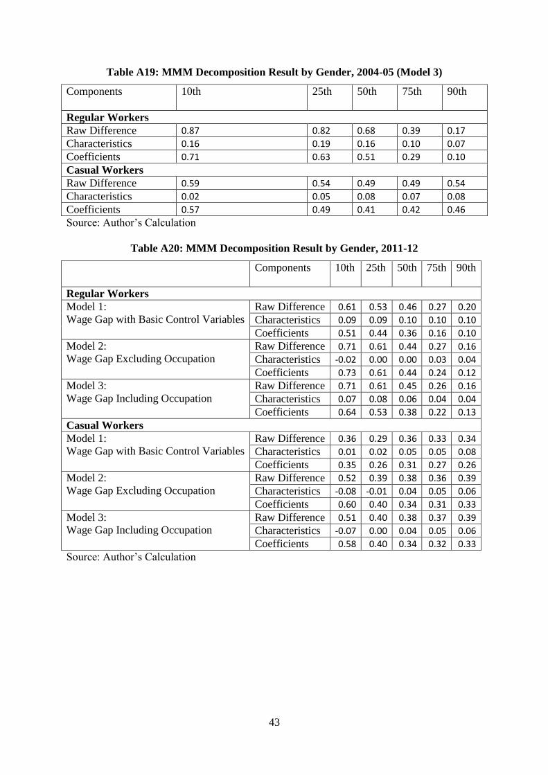
43

Table A19: MMM Decomposition Result by Gender, 2004-05 (Model 3)

Components

10th 25th 50th 75th 90th

Regular Workers

Raw Difference 0.87 0.82 0.68 0.39 0.17

Characteristics 0.16 0.19 0.16 0.10 0.07

Coefficients 0.71 0.63 0.51 0.29 0.10

Casual Workers

Raw Difference 0.59 0.54 0.49 0.49 0.54

Characteristics 0.02 0.05 0.08 0.07 0.08

Coefficients 0.57 0.49 0.41 0.42 0.46

Source: Author‟s Calculation

Table A20: MMM Decomposition Result by Gender, 2011-12

Components

10th 25th 50th 75th 90th

Regular Workers

Model 1:

Wage Gap with Basic Control Variables

Raw Difference 0.61 0.53 0.46 0.27 0.20

Characteristics 0.09 0.09 0.10 0.10 0.10

Coefficients 0.51 0.44 0.36 0.16 0.10

Model 2:

Wage Gap Excluding Occupation

Raw Difference 0.71 0.61 0.44 0.27 0.16

Characteristics -0.02 0.00 0.00 0.03 0.04

Coefficients 0.73 0.61 0.44 0.24 0.12

Model 3:

Wage Gap Including Occupation

Raw Difference 0.71 0.61 0.45 0.26 0.16

Characteristics 0.07 0.08 0.06 0.04 0.04

Coefficients 0.64 0.53 0.38 0.22 0.13

Casual Workers

Model 1:

Wage Gap with Basic Control Variables

Raw Difference 0.36 0.29 0.36 0.33 0.34

Characteristics 0.01 0.02 0.05 0.05 0.08

Coefficients 0.35 0.26 0.31 0.27 0.26

Model 2:

Wage Gap Excluding Occupation

Raw Difference 0.52 0.39 0.38 0.36 0.39

Characteristics -0.08 -0.01 0.04 0.05 0.06

Coefficients 0.60 0.40 0.34 0.31 0.33

Model 3:

Wage Gap Including Occupation

Raw Difference 0.51 0.40 0.38 0.37 0.39

Characteristics -0.07 0.00 0.04 0.05 0.06

Coefficients 0.58 0.40 0.34 0.32 0.33

Source: Author‟s Calculation

44

Table A21: MMM Decomposition Result by Caste, 2004-05 (Model 3)

Components

10th 25th 50th 75th 90th

Regular Workers

Raw Difference -0.29 -0.27 -0.29 -0.27 -0.24

Characteristics -0.17 -0.15 -0.18 -0.21 -0.20

Coefficients -0.12 -0.12 -0.12 -0.07 -0.04

Casual Workers

Raw Difference 0.03 0.01 -0.02 -0.07 -0.12

Characteristics 0.03 0.01 -0.01 -0.04 -0.06

Coefficients 0.00 0.00 -0.01 -0.03 -0.06

Source: Author‟s Calculation

Table A22: MMM Decomposition Result by Caste, 2011-12

Components 10th 25th 50th 75th 90th

Regular Workers

Model 1:

Wage Gap with Basic Control Variables

Raw Difference -0.18 -0.23 -0.31 -0.30 -0.26 Characteristics -0.16 -0.19 -0.24 -0.23 -0.20 Coefficients -0.02 -0.04 -0.07 -0.06 -0.06

Model 2:

Wage Gap Excluding Occupation

Raw Difference -0.19 -0.25 -0.29 -0.28 -0.24 Characteristics -0.15 -0.17 -0.19 -0.20 -0.19 Coefficients -0.04 -0.08 -0.10 -0.07 -0.05

Model 3:

Wage Gap Including Occupation

Raw Difference -0.20 -0.24 -0.29 -0.28 -0.23 Characteristics -0.17 -0.19 -0.22 -0.23 -0.20 Coefficients -0.02 -0.06 -0.07 -0.05 -0.03

Casual Workers

Model 1:

Wage Gap with Basic Control Variables

Raw Difference 0.06 0.04 0.02 -0.03 -0.12 Characteristics -0.01 -0.02 -0.03 -0.04 -0.05 Coefficients 0.07 0.06 0.05 0.02 -0.07

Model 2:

Wage Gap Excluding Occupation

Raw Difference 0.05 0.02 -0.02 -0.08 -0.15 Characteristics 0.02 0.00 -0.03 -0.06 -0.10 Coefficients 0.03 0.02 0.01 -0.02 -0.05

Model 3:

Wage Gap Including Occupation

Raw Difference 0.05 0.02 -0.02 -0.08 -0.15 Characteristics 0.02 0.00 -0.03 -0.06 -0.10 Coefficients 0.03 0.02 0.01 -0.02 -0.05

Source: Author‟s Calculation

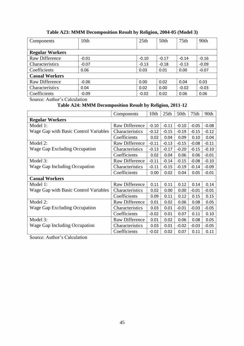
45

Table A23: MMM Decomposition Result by Religion, 2004-05 (Model 3)

Components

10th 25th 50th 75th 90th

Regular Workers

Raw Difference -0.01 -0.10 -0.17 -0.14 -0.16

Characteristics -0.07 -0.13 -0.18 -0.13 -0.09

Coefficients 0.06 0.03 0.01 0.00 -0.07

Casual Workers

Raw Difference -0.06 0.00 0.02 0.04 0.03

Characteristics 0.04 0.02 0.00 -0.02 -0.03

Coefficients -0.09 -0.02 0.02 0.06 0.06

Source: Author‟s Calculation

Table A24: MMM Decomposition Result by Religion, 2011-12

Components 10th 25th 50th 75th 90th

Regular Workers

Model 1:

Wage Gap with Basic Control Variables

Raw Difference -0.10 -0.11 -0.10 -0.05 -0.08

Characteristics -0.12 -0.15 -0.19 -0.15 -0.12

Coefficients 0.02 0.04 0.09 0.10 0.04

Model 2:

Wage Gap Excluding Occupation

Raw Difference -0.11 -0.13 -0.15 -0.08 -0.11

Characteristics -0.13 -0.17 -0.20 -0.15 -0.10

Coefficients 0.02 0.04 0.06 0.06 -0.01

Model 3:

Wage Gap Including Occupation

Raw Difference -0.11 -0.14 -0.15 -0.08 -0.10

Characteristics -0.11 -0.15 -0.19 -0.14 -0.09

Coefficients 0.00 0.02 0.04 0.05 -0.01

Casual Workers

Model 1:

Wage Gap with Basic Control Variables

Raw Difference 0.11 0.11 0.12 0.14 0.14

Characteristics 0.02 0.00 0.00 -0.01 -0.01

Coefficients 0.09 0.11 0.12 0.15 0.15

Model 2:

Wage Gap Excluding Occupation

Raw Difference 0.01 0.02 0.06 0.08 0.05

Characteristics 0.03 0.01 -0.01 -0.03 -0.05

Coefficients -0.02 0.01 0.07 0.11 0.10

Model 3:

Wage Gap Including Occupation

Raw Difference 0.01 0.02 0.06 0.08 0.05

Characteristics 0.03 0.01 -0.02 -0.03 -0.05

Coefficients -0.02 0.02 0.07 0.11 0.11

Source: Author‟s Calculation

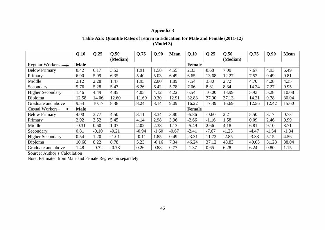
46

Appendix 3

Table A25: Quantile Rates of return to Education for Male and Female (2011-12)

(Model 3)

Q.10 Q.25 Q.50

(Median)

Q.75 Q.90 Mean Q.10 Q.25 Q.50

(Median)

Q.75 Q.90 Mean

Regular Workers Male Female

Below Primary 8.42 6.17 3.52 1.91 1.58 4.55 2.33 8.68 7.00 7.67 4.93 6.49

Primary 6.90 5.99 6.35 5.40 5.03 6.49 6.65 13.68 12.27 7.52 9.49 9.81

Middle 2.12 2.28 1.47 1.95 2.00 1.89 7.54 3.80 2.72 4.70 4.28 4.35

Secondary 5.76 5.28 5.47 6.26 6.42 5.78 7.06 8.31 8.34 14.24 7.27 9.95

Higher Secondary 1.46 4.49 4.85 4.05 4.12 4.22 6.54 10.00 18.99 5.93 5.28 10.68

Diploma 12.58 14.06 12.60 11.69 9.30 12.91 32.83 37.90 37.13 14.21 9.78 30.04

Graduate and above 9.54 10.17 8.38 8.24 8.14 9.09 16.22 17.39 16.69 12.56 12.42 15.60

Casual Workers Male Female

Below Primary 4.00 3.77 4.50 3.11 3.34 3.80 -5.86 -0.60 2.21 5.50 3.17 0.73

Primary 2.92 3.52 5.45 4.14 2.98 3.96 -2.66 -1.16 1.58 0.09 2.46 0.99

Middle -0.31 0.60 1.07 2.02 2.38 1.13 -5.49 2.66 4.18 6.81 9.10 3.71

Secondary 0.81 -0.10 -0.21 -0.94 -1.60 -0.67 -2.41 -7.67 -1.23 -4.47 -1.54 -1.84

Higher Secondary 0.54 1.20 -1.01 -0.11 1.85 0.49 23.31 11.72 -2.85 -3.33 5.15 4.56

Diploma 10.68 8.22 8.78 5.23 -0.16 7.34 46.24 37.12 48.83 40.03 31.28 38.04

Graduate and above 1.48 -0.72 -0.78 0.26 0.88 0.77 -1.37 0.65 6.28 6.24 0.80 1.15

Source: Author‟s Calculation Note: Estimated from Male and Female Regression separately

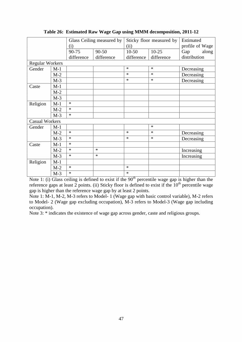
47

Table 26: Estimated Raw Wage Gap using MMM decomposition, 2011-12

Glass Ceiling measured by

(i)

Sticky floor measured by

(ii)

Estimated

profile of Wage

Gap along

distribution 90-75

difference

90-50

difference

10-50

difference

10-25

difference

Regular Workers

Gender M-1 * * Decreasing

M-2 * * Decreasing

M-3 * * Decreasing

Caste M-1

M-2

M-3

Religion M-1 *

M-2 *

M-3 *

Casual Workers

Gender M-1 *

M-2 * * * Decreasing

M-3 * * * Decreasing

Caste M-1 *

M-2 * * Increasing

M-3 * * Increasing

Religion M-1

M-2 * *

M-3 * *

Note 1: (i) Glass ceiling is defined to exist if the 90th

percentile wage gap is higher than the

reference gaps at least 2 points. (ii) Sticky floor is defined to exist if the 10th

percentile wage

gap is higher than the reference wage gap by at least 2 points.

Note 1: M-1, M-2, M-3 refers to Model- 1 (Wage gap with basic control variable), M-2 refers

to Model- 2 (Wage gap excluding occupation), M-3 refers to Model-3 (Wage gap including

occupation).

Note 3: * indicates the existence of wage gap across gender, caste and religious groups.

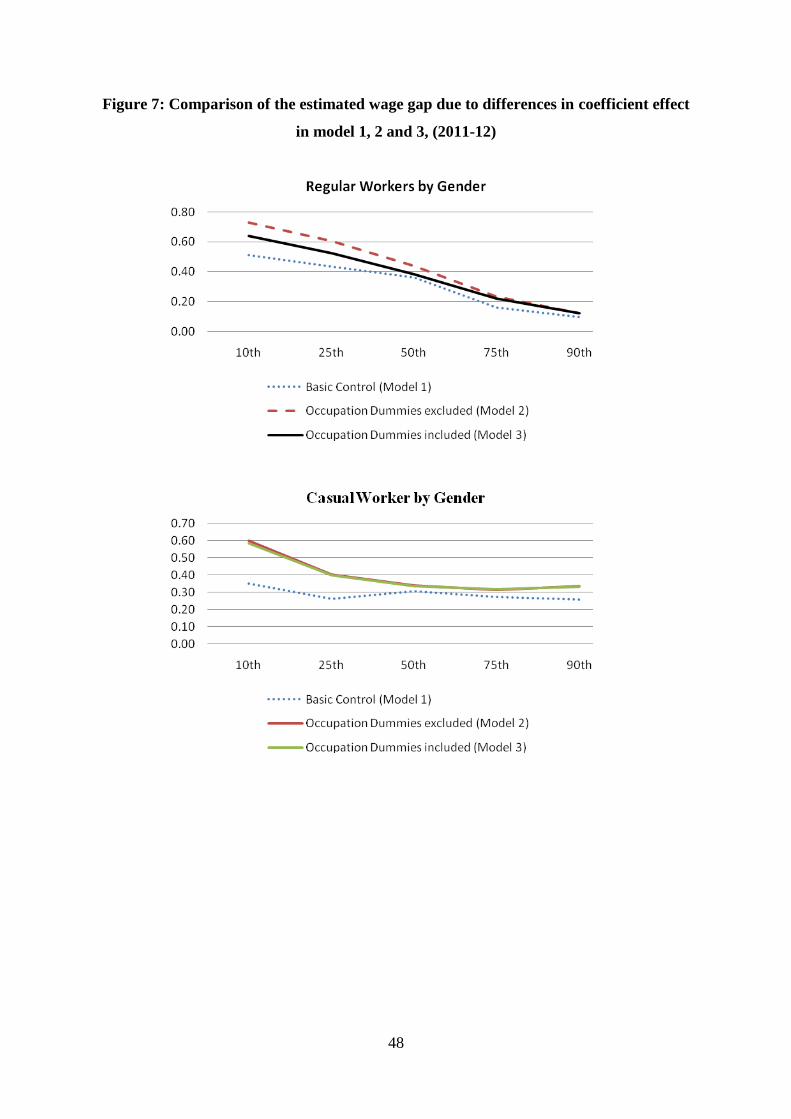
48

Figure 7: Comparison of the estimated wage gap due to differences in coefficient effect

in model 1, 2 and 3, (2011-12)

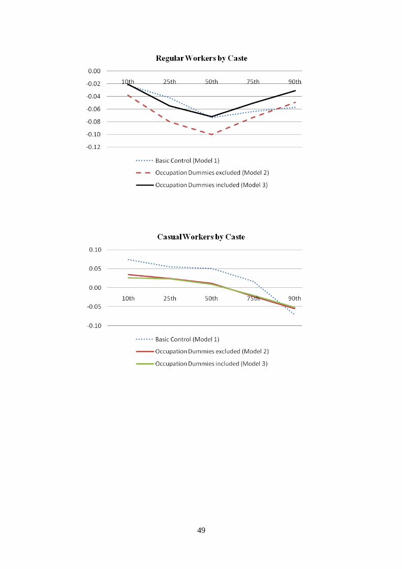
49

50

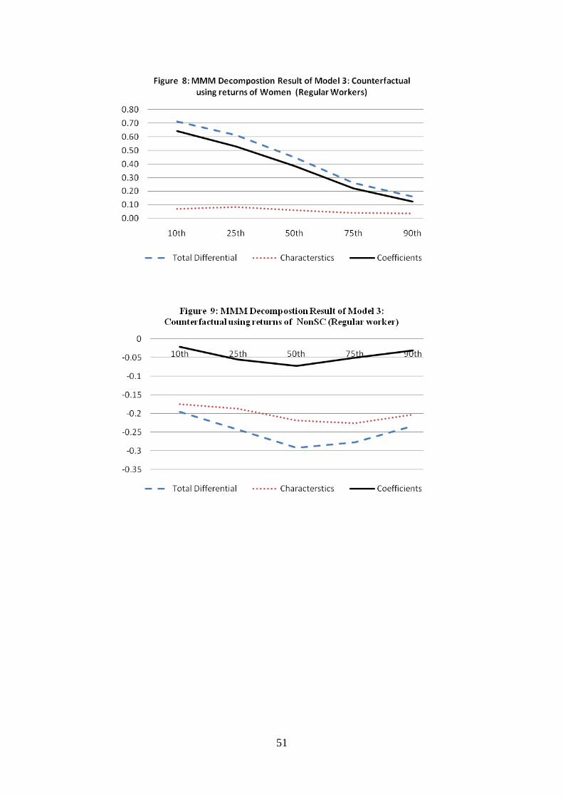
51

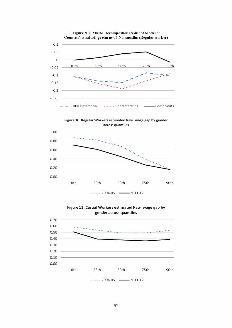
52

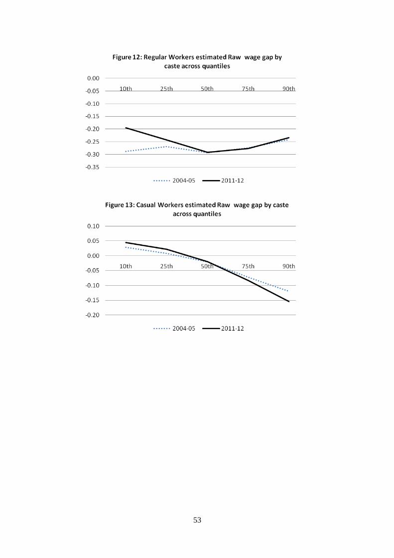
53

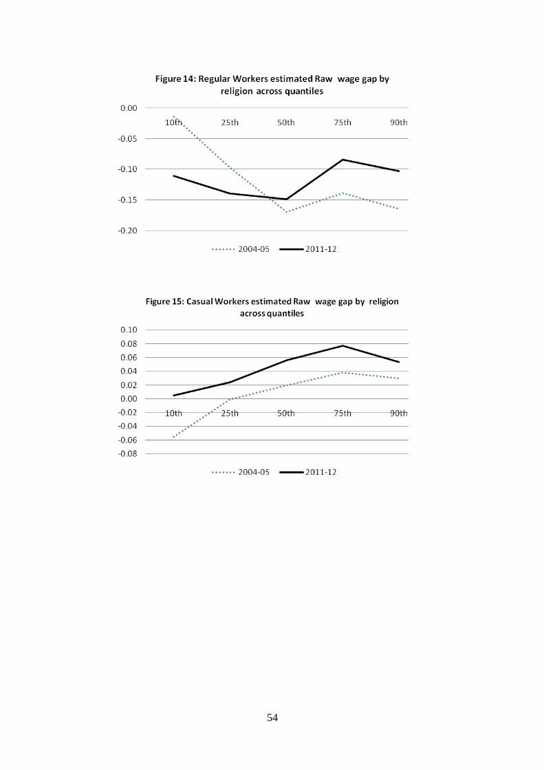
54