is the bimodal oscillating adriatic-ionian circulation a ... · is the bimodal oscillating...

Bollettino di Geofisica Teorica ed Applicata Vol. 57, n. 3, pp. 275-285; September 2016

DOI 10.4430/bgta0176

275

Is the bimodal oscillating Adriatic-Ionian circulation a stochastic resonance?

F. CrisCiani1 and r. Mosetti2

1 Department of Physics, University of Trieste, Italy2 Istituto Nazionale di Oceanografia e di Geofisica Sperimentale - OGS, Trieste, Italy

(Received: October 21, 2015; accepted: April 14, 2016)

ABSTRACT Theobservedpseudoperiodicreversaloftheupper-layercirculationoftheIonianSeahasbeenassumedtoberelatedtosomeinternalfeedbackprocesses(densitydriven)bytheso-calledBiOS(Adriatic-IonianBimodalOscillatingSystem)hypothesis.TheideabehindthispaperisthattheIoniancirculationisdrivenbywhathappensintheboundaryoftheregion,andsoaverysimpledynamicalmodelhasbeenderivedbyintegrating in the bounded flow domain (the Ionian Basin) on the f-plane of the two-layer quasi-geostrophic evolution equations. Furthermore, a nonlinear term whichmimics the mutual interaction between the moving layers has been introduced. Byconsidering a stochastic Gaussian noise acting as a forcing and a decadal periodicinput termhaving an amplitudemuch smaller than thenoisevariance, a stochasticresonanceappearsinthesolutionforacertainrangeofthevaluesoftheparameters.Thedecadal forcingat theboundaryof the Ionianbasincanbe related to the low-frequencyatmosphericvariabilityinthesurroundingbasins.Theresonancehasaperiodconsistentwiththeobserveddecadaltimescaleofthereversalbetweencyclonicandanti-cyclonicphases.

Key words: Watercirculation,dynamicmodel,AdriaticSea,IonianSea.

© 2016 – OGS

1. Introduction

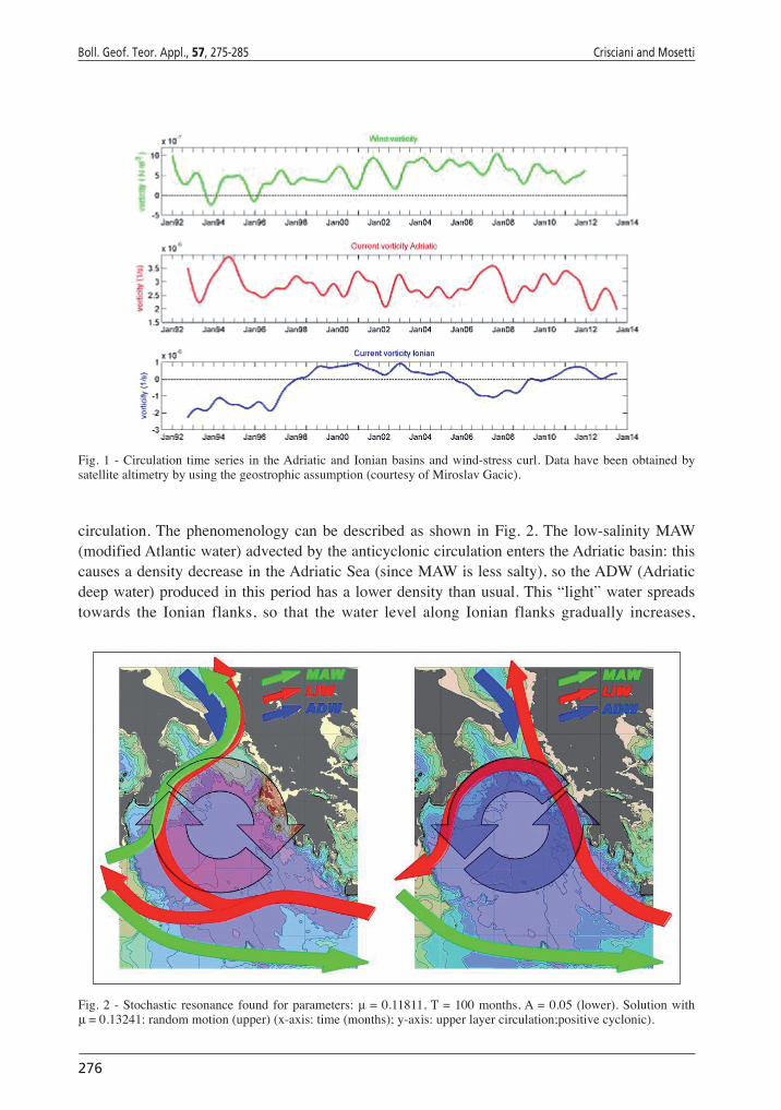
In recent years, the conjecture that theAdriatic-Ionian basin behaves like a bimodaloscillating system, between cyclonic and anticyclonic upper-layer circulation, has been takenintoaccounttoexplainsomeobservationalfacts(Fig.1).

This mechanism is called BiOS. [Adriatic-Ionian Bimodal Oscillating System; Civitarese et al. (2010),Gacicet al. (2010)].BiOS is anewanddifferentwayof explaining the Ionianalternanceinthecirculationbetweencyclonicandanti-cyclonicstates,becauseitattributesitscauses to internalprocessesmore than toexternalones (suchaswindstress). In fact, lookingat Fig. 1, it is clear that the wind-stress curl is unable to reverse the circulation. BiOS cangiveamoregeneralexplanationfor thephenomenon,basedonan“intrinsic”pseudo-periodicoscillation. In addition, the overall surface circulation of theAdriatic Sea is always cyclonic,and salinity and density data collected in the southernAdriatic (the main source of easternMediterraneandeepwater)showadecadalvariationcoherentwiththenorthernIonianchangeinsealevelheight,andingeneral, theirperiodicinversioniscompatiblewiththeinversionof

276

Boll. Geof. Teor. Appl., 57, 275-285 Crisciani and Mosetti

Fig.1 -Circulation timeseries in theAdriaticandIonianbasinsandwind-stresscurl.Datahavebeenobtainedbysatellitealtimetrybyusingthegeostrophicassumption(courtesyofMiroslavGacic).

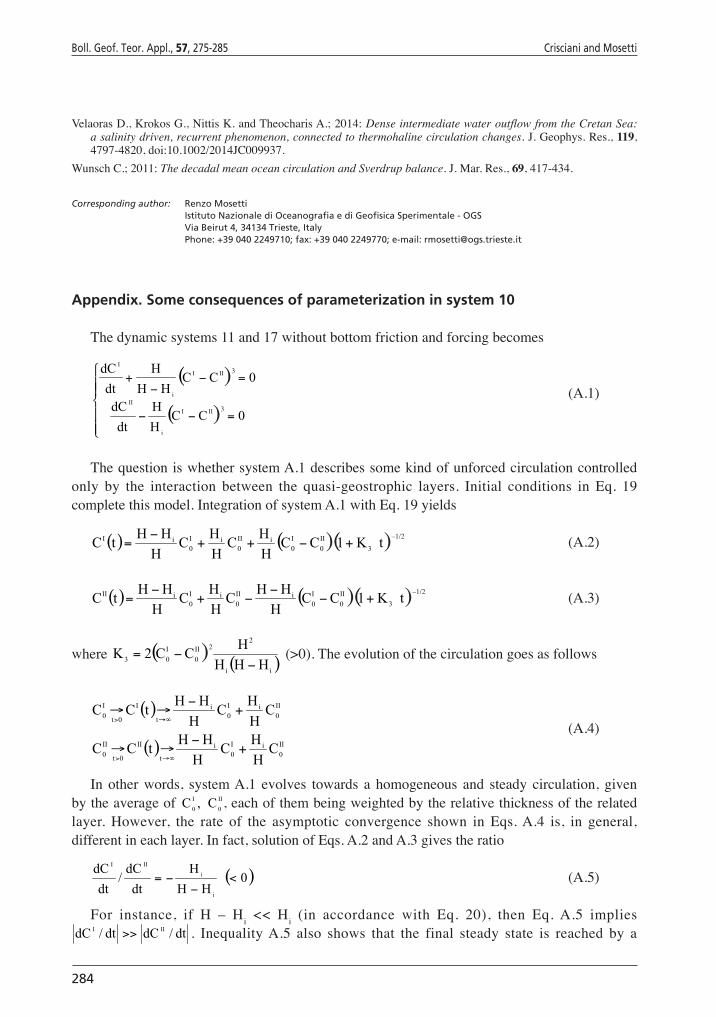
circulation.Thephenomenologycanbedescribedas shown inFig.2.The low-salinityMAW(modifiedAtlanticwater)advectedbytheanticycloniccirculationenterstheAdriaticbasin:thiscausesadensitydecreaseintheAdriaticSea(sinceMAWislesssalty),sotheADW(Adriaticdeepwater)producedinthisperiodhasalowerdensitythanusual.This“light”waterspreadstowards the Ionian flanks, so that the water level along Ionian flanks gradually increases,

Fig. 2 - Stochastic resonance found for parameters: μ = 0.11811, T = 100 months, A = 0.05 (lower). Solution withμ = 0.13241: random motion (upper) (x-axis: time (months); y-axis: upper layer circulation;positive cyclonic).

Is the bimodal oscillating Adriatic-Ionian circulation a stochastic resonance? Boll. Geof. Teor. Appl., 57, 275-285

277

generatinganupwellingofthedenserwaterofthelowerlayers(andaconsequentdownwellingofisobars).Thisleadstoaweakeningoftheanticyclonicupper-layercirculation,whichattheendgetsinverted.ThecyclonicregimefavorsLIW(Levantineintermediatewater)toentertheAdriatic, causingdeepwaters tobe saltier, and thusheavier.Asbefore, denserADWspreadsalong Ionian flanks increasing their density: this causes a gradual downwelling of the upperlighterdensitywater (andaconsequentupwellingof isobars)andagradualweakeningof thecyclonicregime,whichisalso,then,inverted.

Contextualizing to the time interval, in 1994, the anticyclonic gyre extended over the northern Ionian, advecting MAW into the Adriatic (low salinity water). In 1995, anticyclonic gyre became less and less strong and, in 1998, a cyclonic circulation was established. The salinityintheAdriaticbasinstartedtoincreaseagain,sincesaltierLIWwasnowadvectedintoit,asisevidentinFig.2.ItisimportanttounderlinethattheanticyclonictrendadvectsmostlyMAW,sincethepathwayfollowedbywatersistowardsthewesternborderoftheIonian.Ontheotherhand,thecyclonicmotioninduceswatersmostlyontheeasternpartoftheIonian,pushingwaters saltier than MAW into theAdriatic basin.The inversion occurred in 1997, in fact,between 1998 and 2005 a cyclonic gyre was observed, and this caused salty Levantine or Cretan watertoenter,invertingthesaltcontentoftheADWformeduntilnow.Anotherinversionstartedin2006.Currently,thecirculationseemstobeinacyclonicphase(seeagainFig.1).

2. Model equations

In this section, we derive the nondimensional, two-layer quasi-geostrophic model [seeCavallini and Crisciani (2013), for full details of this section], which will be used in a suitable integrated form.With reference to the f – plane1 and in standard notation, in both layers thegoverningequationhastheform:

( ) ψ∇+∂∂

=ψ∇ψ+ψ∇∂∂ − 41122 Re

zw

,Jt

(1)

EachlayerextendsoveraboundedandsimplyconnectedfluiddomainDofthe(x,y)plane.Consider first the upper layer (superscript “I”) included between the rigid lid in z = 1

and the impermeable interface below z = 1, say in zi = (Hi + h)/H. According to this notation,z* = H is the dimensional top of the whole fluid body at rest, while z* = H + h (< H) is the dimensional interface between the moving layers, where h (<< Hi)isthefluctuatingpartoftheinterface.Becauseofmassconservationandbecauseoftheimpermeabilityoftheinterface

∫Dhdxdy = 0 (2)

Thus, vertical integration of Eq. 1 over the mean depth (H – Hi)/H of upper layer yields

( ) ( ) ( )[ ] I41i11

i

I2II2 Rezzw1zwHH

H,J

tψ∇+=−=

−=ψ∇ψ+ψ∇

∂∂ − (3)

1 Indeed the final equations (see Eqs. 11 and 17) are not sensitive to a possible β –effect.

278


Because no stress is applied in z = 1, then

w1 (z = 1) = 0. (4)

On the other hand, given that h is related to both the stream functions ψI, ψII by therelationship

( )III0

gULf

h ψ−ψʹ

= (5)

whereg´isreducedgravity,thentheverticalvelocityattheinterfacecanbewrittenas

( ) ( ) ( ) ( )IIIIIIIIIi ,J

tFzzw ψ−ψℑ+⎥⎦

⎤⎢⎣

⎡ ψψ+ψ−ψ∂∂

ε== (6)

whereHgLf

F22

0

ʹ= is the rotational Froude number. The first term at the right hand side of

Eq.6 takes intoaccount theeffectof fluctuationsof the interfaceon itsverticalvelocity.Thesecond term represents the mutual interaction between the moving layers which affects thesame velocity further on. As in the barotropic limit ψI = ψII, in general ( ) 00 =ℑ .This termwillbesuitablyparameterizedaftertheintegrationofthevorticityequationsonD.Keepinginmind Eqs. 3, 4, and 6 and recalling that, up to the first order in ε, w = εw1wehaveafteralittlealgebra,

( )[ ]( )

( ) I41III

i

IIIII20 ReHH

HF

DtD

ψ∇=ψ−ψℑ−ε

+ψ−ψ−ψ∇ − (7)

where, in the upper layer, ( )⋅ψ+∂∂

= ,JtDt

D I0 and( )i

220I

HHgLf

F−ʹ

= .At this point, by usingReynolds’transporttheorematthelefthandsideandthedivergencetheoremattherighthandside,Eq7canbeintegratedover D togive

(8)

Setting

∫∫∂∂

⋅=⋅=D

IIII

D

II dsˆC,dsˆC tutu (9)

where C is the circulation of the geostrophic current u ψ∇×= k̂u along the unique boundary�D of the fluid domain, we have ∫ =ψ∇

D

II

dtdC

dxdydtd 2 and, because of Eqs. 2 and 5,


279

�(ψI – ψII) dxdy = 0. As anticipated, the parameterization of ∫ ℑD

dxdy isnowassumedintheform

( ) ( )3III

D

III CCdxdy1

−=ψ−ψℑε ∫

(10)

SomeconsequencesofEq.10inthepresentcontextarediscussedintheAppendix.Finally,thefluxofrelativevorticity I2ψ∇ acrosstheboundaryofthedomain,thatis

( )∫∂

⋅ψ∇∇D

I2 dsn̂

isprescribed in termsofagiven functionof timeonly, sayφ (t) .This termcomes from thelateral action of the surrounding flow which forces the upper layer at its boundary. On thewhole, Eq. 8 yields

( )( ) ( )tCC

HHH

dtdC 3III

i

I

ϕ=−−

+ (11)

Consider now the lower layer (superscript “II”) included between the interface in z = ziand the bottom in z = η* / H = η. Vertical integration of Eq. 1 over the mean depth Hi / H of the lowerlayeryields

( ) ( ) ( )[ ] II411i1

i

II2IIII2 RezwzzwHH

,Jt

ψ∇+η=−==ψ∇ψ+ψ∇∂∂ − (12)

wheretheverticalvelocityisagaingivenbyEq.6and

( ) ( ) II2vII1 2

E,FJzw ψ∇

ε+ηψ=η= (13)

Eq. 13 is nothing but the nondimensional version of Eq. 4.9.36 of Pedlosky (1987). By using Eqs. 6 and 13 into Eq. 12, after a little algebra, one obtains

( )[ ] ( ) ( )

II41II2v

i

IIII

i

III

i

IIIIIII20

Re2

E

HH

,JFHH

HH

FDtD

ψ∇=ψ∇ε

+

ηψ+ψ−ψℑε

−ψ−ψ−ψ∇

−

(14)

where, in the lower layer, ( )⋅ψ+∂∂

= ,JtDt

D II0 andi

220II

HgLf

Fʹ

= . Eq. 14 can be integrated on thedomain D along the same lines as Eq. 8 and noting also that, because of Stoke’s theorem,

( ) ∫∫∫∂∂

=⋅η∇ψ=⋅×η∇ψ=ηψD

II

D

II

D

II 0dst̂dsn̂k̂dxdy,J (15)

where IIψ is the constant value taken by the stream function on the boundary. Eq. 15 shows that the model is not sensitive to bottom topography. Hence, integration of Eq. 14 over D yields

( ) ( )∫∂

− ⋅ψ∇∇=ε

+−−D

II21IIv

i

3III

i

II

dsn̂ReC2

E

HH

CCHH

dtdC

(16)

)3

)3 φ

( )[ ] ( ) ( )

II41II2v

i

IIII

i

III

i

IIIIIII20

Re2

E

HH

,JFHH

HH

FDtD

ψ∇=ψ∇ε

+

ηψ+ψ−ψℑε

−ψ−ψ−ψ∇

−

)3

280


The line integralat the righthandsideofEq.16 is the fluxof relativevorticitycrossing theboundary of the lower layer, which has the same meaning as that of the upper layer. However, unliketheupperlayer,thisfluxisprescribedtobeaconstant(sayφ0),sothefinalformofEq.16is

( ) 0IIv

i

3III

i

II

C2

E

HH

CCHH

dtdC

ϕ=ε

+−− (17)

Notethat

ε=

ε 2

1

H

H

2

E

H

H

i

Ev

i

(18)

where HEisthethicknessoftheEkmanbenticlayer.Accordingtotheordersofmagnitude(inS.I.units)consistentwiththisinvestigationandlistedbelow

HE = O(10), Hi = O (3.5×103), U = O (5×10-2), L = O (5×105)

the quantity in Eq. 18 is O(1). To summarize, the coupled Eqs. 11 and 17 give the time evolution of the circulation in both fluid layers once all the inputs are established and definite initialconditions

( ) ( ) II0

III0

I C0C,C0C == (19)

arefixed.Inwhatfollows,thevalues(inS.I.units)

12

E

H

H,105.3H,104H v

i

3

i

3 =ε

×=×= (20)

willbeadopted,whileφ(t)andφ0willbechosenwithintheframeworkofstochasticresonance,sotheconstantsinEq.19areexpectedtoplayaminorroleinthelong-termbehaviourofEq.9.

3. The stochastic resonance hypothesis

The mechanism of stochastic resonance was introduced in a seminal paper (Benzi et al., 1981). They discovered that a stochastic system (having motion in all time scales) forced by a periodicsignalmaycreateinthesolutionabi-stableresponsecharacterizedbyarapidtransitionbetween the two states with the same period of the forcing term. Since the discovery, theconceptofstochasticresonancehasbeenwidelyappliedtoseveraldisciplinesinthecontextofdynamicalsystemsandinparticulartoclimatedynamics(e.g.,Benzi et al., 1982). Furthermore, stochastic resonance has been investigated in the framework of the Stommel thermohalinemodel(Eyink, 2005).

The idea is to explore if thedynamical systemdescribedbyEqs. 11 and17 could exhibita stochastic resonance when a periodic decadal forcing and a random noise are introduced.BecausetheBiOSprocessissupposedtobeabi-stablesystem,thestochasticresonancecouldbeacandidatemodel toexplain theobservedpseudo-periodic reversalof the Ionianvorticity.

)3 φ


281

Notice that in the framework of this model, the forcing is acting on the boundary region ofthe Ionian Sea.This forcing derives from the lateral action of the surrounding flows.Theintroductionofadecadalperiodicityintothesystemcanbesupportedbythefactthatlarge-scaleoceanprocesses are influencedbyatmospheric forcingand the appearanceof adecadal scaleis quite common (Cessi and Louazel, 2001; Wunsch, 2011, Kondrashov and Berloff, 2015). Followingtheseconsiderations,wemodifythesystemofEqs.11,and17asfollows:

( )( ) )t(s)T/t2sin(A)t(CC

HHH

dtdC 3III

i

I

μ+π=ϕ=−−

+

( ) 0C2

E

H

HCC

H

H

dt

dC IIv

i

3III

i

II

=ε

+−−

(21)

where A is the amplitude of the forcing; T is the period (decadal); μs(t) is a Gaussian noise process physically representing the high-frequency signal (time scales from the monthly/seasonaltotheinterannual)oftheforcingactingontheboundaryregion.

The numerical integration of the stochastic system 21 has been made by means of aMATLAB code based on the Runge-Kutta ODE solver.A large set of runs have been doneby small changes in the variance of the random noise since the stochastic resonance usuallyappears within a very narrow range of variance (Fig. 3). As can be seen in Fig. 3, the solutions are stronglysensitive to the ratiobetween theperiodicamplitudeand thenoisevariance.Thestochastic resonance can be found, being A= 0.05, in a range between μ = 0.115 and μ = 0.120.

Noticethat,despitetheweaknessoftheperiodicforcingwithrespecttothenoisevariance,the solution shows stochastic transitions which are correlated to the period of 100 monthspresent in the forcing. Note also that the average time duration of a cyclonic or anticyclonicphaseisone-halfoftheperiod(withthetransitiontimemuchshorterbetweenthetwostates).This is a typical behaviour of a stochastic resonance. In other words, the mean residence time τ of the stable states is related to the period T by the relation T � 2 τ.

)3 φ

)3

Fig. 3 - The BiOS mechanism (after Civitareseet al.,2010).

282


4. Discussion

ThedrivingmechanismsbehindthedecadalreversaloftheIonianSeaupper-layercirculationprovoked a considerable debate in the Mediterranean scientific community. It is still unclearwhatthedrivingforceis.Ithasbeensuggestedthatthereversalcouldbedrivenbyvariationsin wind-stress curl over the basin, baroclinic dynamics acting within theAdriatic-IonianSystem (AIS), or baroclinic dynamics driven by thermohaline properties at theAIS easternboundary.The variability observed in the Ionian circulation has been often associated with achange in the wind-stress curl over the area (Pinardi et al., 1997, 2015). Recently, Theocharis et al. (2014) suggested that the decadal variability observed in the Ionian circulation reflects aninternalmechanismdrivingthealternationoftheAdriaticSeaandtheAegeanSeaasmainDWF (deepwater formation) sites for the easternMediterranean (EMED).This thermohalinepumping (Theocharis et al., 2014; Velaoras et al., 2014) involves the whole thermohaline cell of the EMED, and not only theAdriatic-Ionian Sea, as in the BiOS hypothesis (Gacic et al., 2010). In both cases, the role of long term atmospheric forcings has been considerednegligible. In a recent paper by Mihanović et al. (2015), it is claimed that BiOS is the dominant generatoroftheAdriaticdecadalvariability.Onthecontrary,inthepresentpaper,itisassumedthat the upper-layer Ionian circulation is driven by the forcing acting on the boundary of theIonianregionassuggestedbytheschemeofcirculationdepictedinFig.2.In thishypothesis,neitherthebaroclinicitynorthewind-stresscurlinside the Ionian basinareresponsiblefortheinversion of the circulation at decadal time scale.The forcing is due to both interannual anddecadal variability of theAdriatic and the adjacent basins’ meteo-oceanographic conditionsforcing the boundary of the basin (it could also be the effect of theAegean Sea in the caseof the East MediterraneanTransient).The presence of a decadal variability in theAdriaticSea oceanographic condition has been recently shown by, among others, a new analysisof experimental data in the paper by Mihanović et al. (2015). In our opinion, this is due to the corresponding decadal scale in the atmospheric forcing. In this sense, the already citedpaper by Pinardi et al. (2015) reinforces this conjecture, since it gives a clear picture of the mean circulation of the Mediterranean Sea emerging from a 23-year eddy-resolving model reanalysis.Themulti-decadalmean flowemerging from thisanalysis is consistentwithmanyof the previous findings, but new circulation structures also become apparent. It is clearlystated that“TheIonianreversalmechanismisalsoevident in thestreamfunction, thusgivingfurther evidenceof thewind-drivennatureof themechanismsunderlying thenorthern Ionianreversal”. In thepresentapproach,evenif thedecadalatmosphericsignalcouldbeveryweakwithrespecttotheinterannualvariability,itisreflectedintotheboundaryoftheupperlayerofthe Ionian regiondriving thecirculation inversion throughastochastic resonancemechanism.Thehypothesis thatapurely termohalineprocesscouldexplain theIoniancirculationreversalhas also been tested by using a thermohaline (with temperature and salinity state variables)three-layerboxmodelfollowingtheapproachbyAshkenazy et al. (2012),inaMaster’sdegreethesis (Capuano, 2015). By using the typical values for deep-water formation rate in the Adriatic SeaaswellastherealisticvaluesforthefluxesbetweentheAdriaticbox,theIonianbox,andtheeasternMediterraneanbox,noperiodicsolutionsappear,andsothereisnopossiblereversalof the Ionian gyre in the upper layer (500 m). In this sense, the model developed here moves toapossibleconclusion thatBiOSisa forcedmechanisminducedby the typicalatmospheric


283

decadal scales. It is still not clear if the decadal variability is connected, for example, to theNAOindexortosomeotheratmosphericteleconnectionsintheMediterraneanarea.

Themodeldevelopedheredoesnothaveanyrelationtothedeepwaterformationprocesses.As speculated in the above-cited paper by Mihanović et al. (2015), the dense water outflowrates from the Adriatic through the Otranto Strait (-0.3 Sv) does not have the capacity to rapidly invertthecirculationintheupperIonianSea.Onthecontrary,thestochasticresonanceshows,asatypicalfeature,rapidswitchesfromoneregimetotheother. However, due to the detailed knowledge of the thermohaline structure of theAdriatic-Ionian basins coming from longtimeCTDdata,furtherimprovementscouldbeexpectedbyusingaquasi-geostrophiccontinuouslystratifiednumericalmodeltoinvestigatetheroleofbaroclinicityandthatoftheAdriaticdeepwater.

Acknowledgements. Theauthorsgratefullythanktheircolleaguedr.FabioCavalliniforausefuldiscussionaboutmathematicalaspectsoftheinvestigation.Thanksalsotodr.MiroslavGacicforhiscommentsontheBiOSphenomenology.

REFERENCES

Ashkenazy Y., Stone P.H. and Malanotte-Rizzoli P.; 2012: Box modeling of the Eastern Mediterranean sea. Phys. A: StatisticalMechanimsanditsApplications,391, 1519-1531.

Benzi R., Sutera A. and Vulpiani A.; 1981: The mechanism of stochastic resonance. J. Phys. A: Math. Gen., 14, L453-L457.

Benzi R., Parisi G., Sutera A. and Vulpiani A.; 1982: Stochastic resonance in climate change.Tellus,34,10-16.Capuano C.; 2015: Non-linear box models for the study of the interannual variability of the thermohaline parameters

of Adriatic-Ionian basin. University of Trieste, Inter athenaeum Master’s Degree in Physics - Earth and Environmental Physics Curriculum, Academic Year 2013-2014. Supervisor: Renzo Mosetti.

Cavallini F. and Crisciani F.; 2013: Quasi-geostrophic theory of oceans and atmosphere:topics in the dynamics and thermodynamics of the fluid earth. Springer, Dordrecht, The Netherlands, 385 pp.

Cessi P. and Louazel S.; 2001: Decadal oceanic response to stochastic wind forcing. J. Phys. Oceanogr., 31, 3020-3029.

CivitareseG.,GacicM.,BorzelliG.L.andLipizerM.;2010:On the impact of the Bimodal Oscillating System (BiOS) on the biogeochemistry and biology of the Adriatic and Ionian Seas (Eastern Mediterranean). Biogeosci., 7,3987-3997.

Eyink G.L.; 2005: Statistical hydrodynamics of the thermohaline circulation in a two-dimensional model.Tellus,57A,100-115.

Gacic M., Borzelli G.L.E., Civitarese G., Cardin V. and Yari S.; 2010: Can internal processes sustain reversals of the ocean upper circulation? The Ionian Sea example.Geophys.Res.Lett.,37,L09606.

Kondrashov D. and Berloff P.; 2015: Stochastic modeling of decadal variability in ocean gyres.Geophys.Res.Lett.,42, 1543-1553, doi:10.1002/2014GL062871.

Mihanović H., Vilibić I., Dunić N. and Sepić J.; 2015: Mapping of decadal middle Adriatic oceanographic variability and its relation to the BiOS regime.J.Geophys.Res.,120, 5615-5630, doi:10.1002/2015JC010725.

Pedlosky J.; 1987: Geophysical fluid dynamics.Springer,NewYork,710pp.Pinardi N., Korres G., Lascaratos A., Roussenov V. and Stanev E.; 1997: Numerical simulation of the interannual

variability of the Mediterranean Sea upper ocean circulation.Geophys.Res.Lett.,24, 425-428.Pinardi N., Zavatarelli M., Adani M., Coppini G., Fratianni C., Oddo P., Simoncelli S., Tonani M., Lyubartsev V.,

Dobricic S. and Bonaduce A.; 2015: Mediterranean Sea large-scale low-frequency ocean variability and water mass formation rates from 1987 to 2007: a retrospective analysis. Prog. Oceanogr., 132, 318-332.

Theocharis A., Krokos G., Velaoras D. and Korres G.; 2014: An internal mechanism driving the alternation of the eastern Mediterranean dense/deep water sources. In: Borzelli G.L.E., Gacic M., Lionello P. and Malanotte-Rizzoli P. (eds), The Mediterranean Sea: temporal variability and spatial patterns, John Wiley, Oxford, U.K., pp. 113-137, doi:10.1002/9781118847572.ch8.

284


Velaoras D., Krokos G., Nittis K. and Theocharis A.; 2014: Dense intermediate water outflow from the Cretan Sea: a salinity driven, recurrent phenomenon, connected to thermohaline circulation changes.J.Geophys.Res.,119,4797-4820, doi:10.1002/2014JC009937.

WunschC.;2011:The decadal mean ocean circulation and Sverdrup balance.J.Mar.Res.,69, 417-434.

Corresponding author: Renzo Mosetti Istituto Nazionale di Oceanografia e di Geofisica Sperimentale - OGS Via Beirut 4, 34134 Trieste, Italy Phone: +39 040 2249710; fax: +39 040 2249770; e-mail: [email protected]

Appendix. Some consequences of parameterization in system 10

Thedynamicsystems11and17withoutbottomfrictionandforcingbecomes

( )

( )⎪⎪⎩

⎪⎪⎨

⎧

=−−

=−−

+

0CCH

H

dt

dC

0CCHH

H

dt

dC

3III

i

II

3III

i

I

(A.1)

ThequestioniswhethersystemA.1describessomekindofunforcedcirculationcontrolledonly by the interaction between the quasi-geostrophic layers. Initial conditions in Eq. 19completethismodel.IntegrationofsystemA.1withEq.19yields

( ) ( )( ) 2/1

3II0

I0

iII0

iI0

iI tK1CCHH

CHH

CH

HHtC

−+−++

−= (A.2)

( ) ( )( ) 2/1

3II0

I0

iII0

iI0

iII tK1CCH

HHC

HH

CH

HHtC −+−

−−+

−= (A.3)

where ( )( )ii

22II

0I03 HHH

HCC2K

−−= (>0).Theevolutionofthecirculationgoesasfollows

( )

( ) II0

iI0

i

t

II

0t

II0

II0

iI0

i

t

I

0t

I0

CHH

CH

HHtCC

CHH

CH

HHtCC

+−

→→

+−

→→

∞→>

∞→>

(A.4)

In other words, systemA.1 evolves towards a homogeneous and steady circulation, givenbytheaverageof II

0

I

0C,C ,eachofthembeingweightedbytherelativethicknessoftherelated

layer. However, the rate of the asymptotic convergence shown in Eqs. A.4 is, in general, different in each layer. In fact, solution of Eqs. A.2 and A.3 gives the ratio

( )0

HH

H

dt

dC/

dt

dC

i

i

III

<−

−= (A.5)

For instance, if H – Hi << Hi (in accordance with Eq. 20), then Eq. A.5 implies dt/dCdt/dC III >> . Inequality A.5 also shows that the final steady state is reached by a

)3

)3

)(( ) ( )( ) 2/1

3II0

I0

iII0

iI0

iI tK1CCHH

CHH

CH

HHtC

−+−++

−= )–1/2

)(( ) ( )( ) 2/1

3II0

I0

iII0

iI0

iI tK1CCHH

CHH

CH

HHtC

−+−++

−= )–1/2

)2


285

decreaseofthecirculationrateinonelayerandtheincreaseintheother.The monotonic character of solution of Eqs. A.2 and A.3 implies that CI(t)revertsitssignat

mostonceinthecourseoftimeifandonlyifCI(0)and ( )tClim I

t +∞→havediscordantsigns,thatis

tosayifandonlyif

0CHH

CH

HHC II

0iI

0iI

0 <⎟⎠

⎞⎜⎝

⎛ +− (A.6)

Forthesamereason,CII(t)revertsitssignatmostonceinthecourseoftimeifandonlyif

0CHH

CH

HHC II

0iI

0iII

0 <⎟⎠

⎞⎜⎝

⎛ +− (A.7)

However, the inversion of the circulation in both layers is not possible, even in deferred times.Infact,bothEqs.A.6andA.7imply

0CC II0

I0 < (A.8)

soCI0andCII

0shouldhaveconcordantsignsbecauseofEqs.A.6andA.7,butdiscordantbecauseof Eq. A.8.

AnotherquestionisthereasonwhyjustthethirdpowerofthedifferenceCI–CIIisintroducedin Eq. 10. Integration of system A.1 with n = 2,3,4... in place of the third power appearing in systemA.1resultsintheequations

( ) ( )( )

( ) ( )( ) n1

1

nII0

I0

iII0

iI0

iII

n1

1

nII0

I0

iII0

iI0

iI

tK1CCH

HHC

HH

CH

HHtC

tK1CCHH

CHH

CH

HHtC

−

−

+−−

−+−

=

+−++−

= (A.9)

where

( )( )( )ii

21nII

0I0n HHH

HCC1nK

−−−=

− (A.10)

Solution of Eqs. A.9 coincides trivially with Eq. A.2 and A.3 for n = 3. Consider the function oftime

( ) ( ) n1

1

n tK1t −+=φ (A.11)

included in the above class of solutions and, owing to the arbitrariness of initial conditions,assumeCI

0–CII0 < 0. The following alternative holds:

1) the integer n is even. Hence Kn < 0 so Eq. A.8 has a singularity for some 0t~ > ;2) the integer n is odd. Hence Kn > 0 so Eq. A.8 is positive definite ∀ 0t ≥ .Becauseofthearbitrarinessofinitialconditions,anevenvalueofnmustberuledoutandthe

smallest odd integer for which the solution exists is n = 3.

)(1+Knt)1

––––––

1–n

)(1+Knt)1

––––––

1–n

)(CI0–C0II)n–1( )( )

( )ii

21nII

0I0n HHH

HCC1nK

−−−=

−

) 1––––––

1–n

is the bimodal oscillating adriatic-ionian circulation a ... · is the bimodal oscillating...

Documents