ioi - nasa

NASA-CR-192281

Final Report

for the period January I, 1990 - June 30, 1992

on

ANALYSIS OF ELECTROMAGNETIC INTERFERENCE FROMPOWER SYSTEM PROCESSENG AND TRANSMISSION

COMPONENTS FOR SPACE STATION FREEDOM

Grant No. NAG3-1126

by

Peter W. Barber

Principal Investigator

and

Nabeel A.O. Demerdash

Co-Principal Investigator

Research Assistants: R. Wang, B. Hurysz, Z. Luo

Department of Electrical and Computer Engineering

Clarkson UniversityPotsdam, NY 13699-5720

--_ lc:-f

IOi

Consultants:Hugh W. Denny, David P. Millard,R. HerkertGeorgia Tech Research Institute

Submitted to

Power Management and DistributionSystems Branch

Mail Stop 500-102NASA - Lewis Research Center

21000 Brookpark Road

Cleveland, OH 44136

(NASA-CR-192281) ANALYSIS OF

ELECTROMAGNETIC INTERFERENCE FROM

POWER SYSTEM PROCESSING ANO

TRANSMISSION COMPONENTS FOR SPACE

STATION FREEO_M Fina] Report, IJan. 1990 - 30 Jun. I992 (C|arkson

Univ.) I01 p G]/18

N93-19890

Uncl as

01_8105

Final Report

for the period January 1, 1990 - June 30, 1992

on

ANALYSIS OF ELECTROMAGNETIC INTERFERENCE FROMPOWER SYSTEM PROCESSING AND TRANSMISSION


Grant No. NAG3-1126

by

Peter W. Barber

Principal Investigator

and

Nabeel A.O. Demerdash

Co-Principal Investigator

ResearchAssistants:R. Wang, B. Hurysz, Z. Luo

Department of Electrical and Computer Engineering

Clarkson University

Potsdam, NY 13699-5720

Consultants: Hugh W. Denny, David P. Millard,R. HerkertGeorgia Tech Research Institute

t !

il

ANALYSIS OF ELECTROMAGNETIC INTERFERENCE FROM

POWER SYSTEM PROCESSING AND TRANSMISSIONCOMPONENTS FOR SPACE STATION FREEDOM

Table of Contents

ua_e

Section 1. Introduction 1

Section 2. Device Models 2

Section 3. Radiation Sources 31

List of Figures

Figure

Figure

Figure

Figure

Figure

Figure

Figure

Figure

Figure

Figure

Figure

Figure

Figure

Figure

Figure

Figure

Figure

Figure

Figure

Figure

2.10

2.11

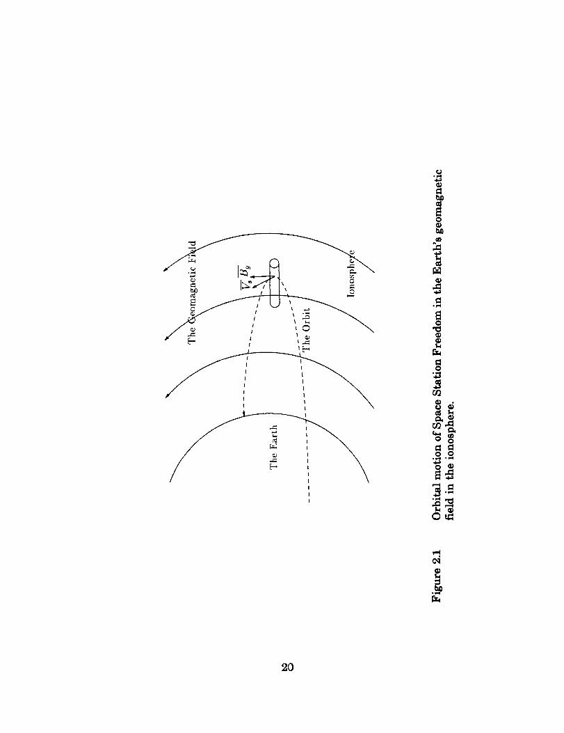
2.1 Orbital motion of Space Station Freedom in the Earth's geomagnetic

field in the ionosphere.

2.2 The partition of the problem region.2.3 The first order tetrahedral surface element and local coordinate.

2.4 The first order tetrahedral element.

2.5 Geometry of the example.

2.6 Tetrahedral element grid for a cylindrical object with a sphere outer

boundary, for NE = 3456, NN = 669.

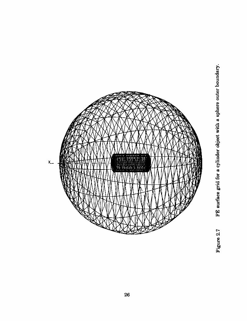
2.7 FE surface grid for a cylinder object with a sphere outer boundary.

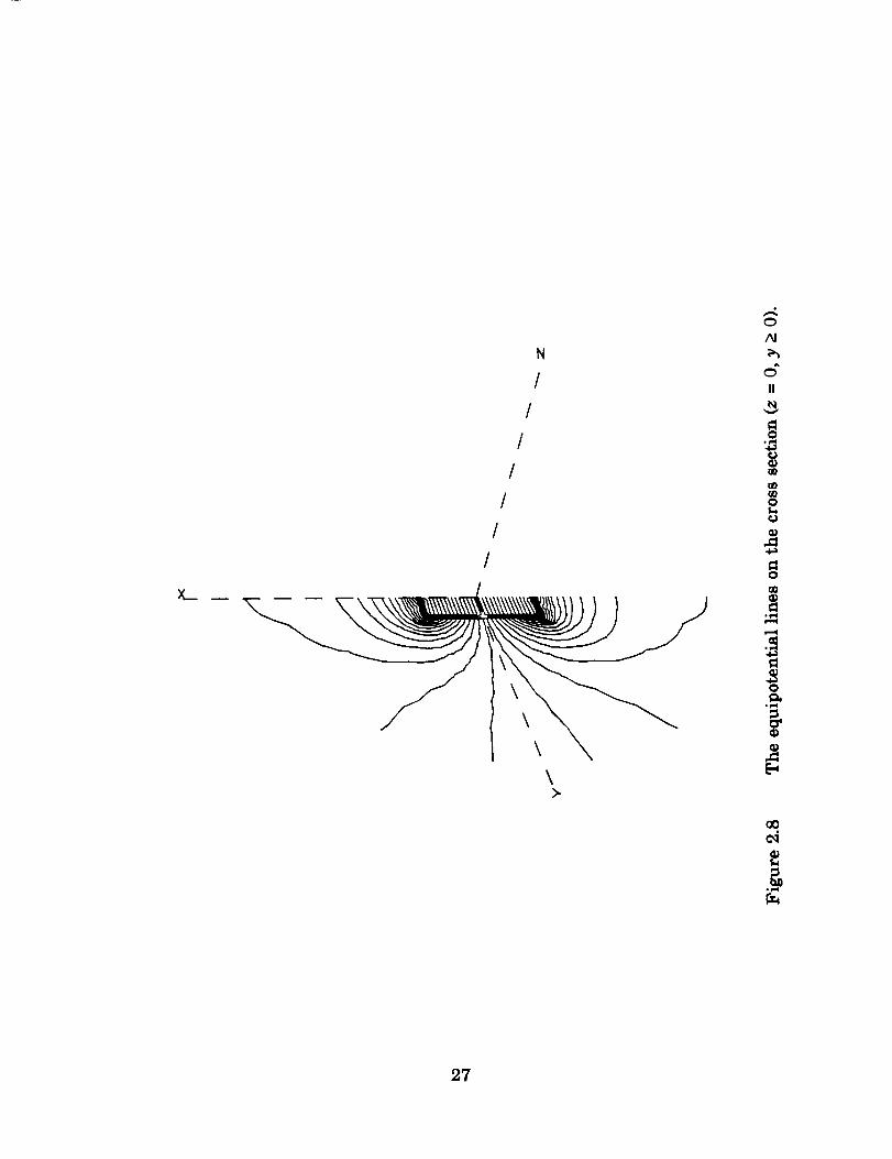
2.8 The equipotential lines on the cross section (z = 0, y > 0).

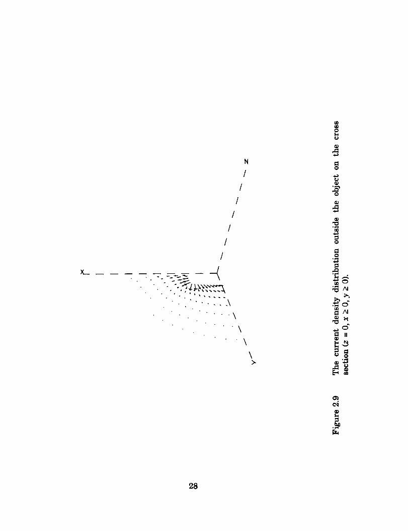
2.9 The current density distribution outside the object on the cross section

(z = 0, x > 0, y > 0).

The current density component J, distribution on plane x = 0 with al =

5.7 x 107 1/fl-m, a2 = 5.7 x 105 1/i2-m.

The scalar potentials on the x-axis with a 1 = 5.7 x 107 1/_-m, a 2 = 5.7 x

105 1/_-m.

3.1 Ionospheric charge density as a function of altitude.

3.2 Plasma frequency fp versus electron density N.3.3 Attenuation vs frequency for specified electron densities.

3.4 Effect of varying the electron density on the electric field.

3.5 Wire model with a short monopole antenna excited at one end.

3.6 Current along a 100 m wire with a monopole source at one end.

3.7 Simple wire model of Space Station Freedom.

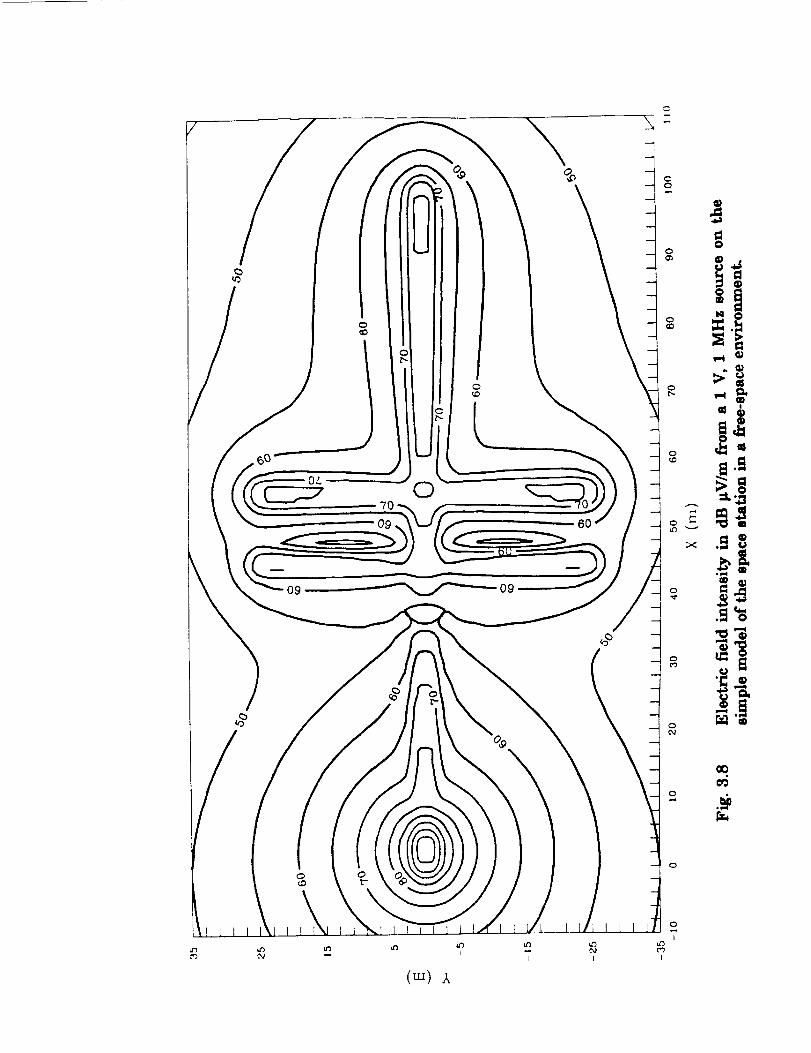
3.8 Electric field intensity in dB _V/m from a 1 V, 1 MHz source on the

simple model of the space station in a free-space environment.

3.9 Electric field intensity in dB _tV/m from a 1 V, 1 MHz source on the

simple model of the space station in a zero-order plasma environment.

°°o

Ul

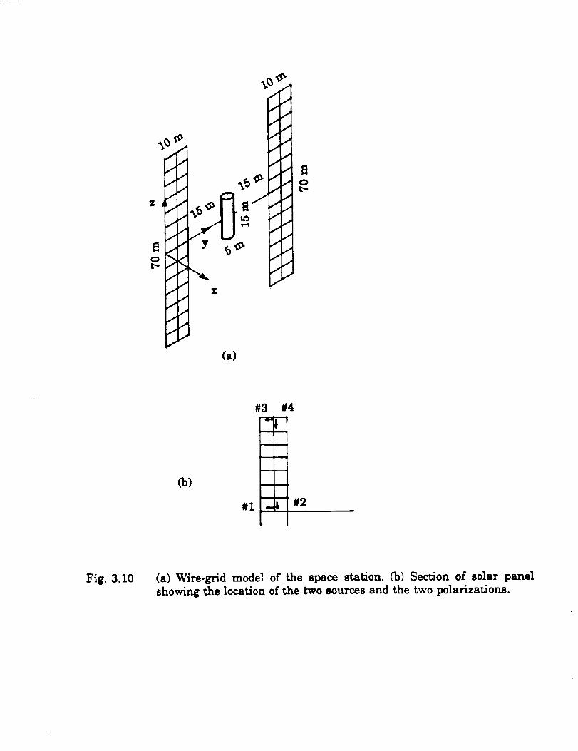
Figure 3.10 (a) Wire-grid model of the space station. (b) Section of solar panelshowing the location of the two sources and the two polarizations.

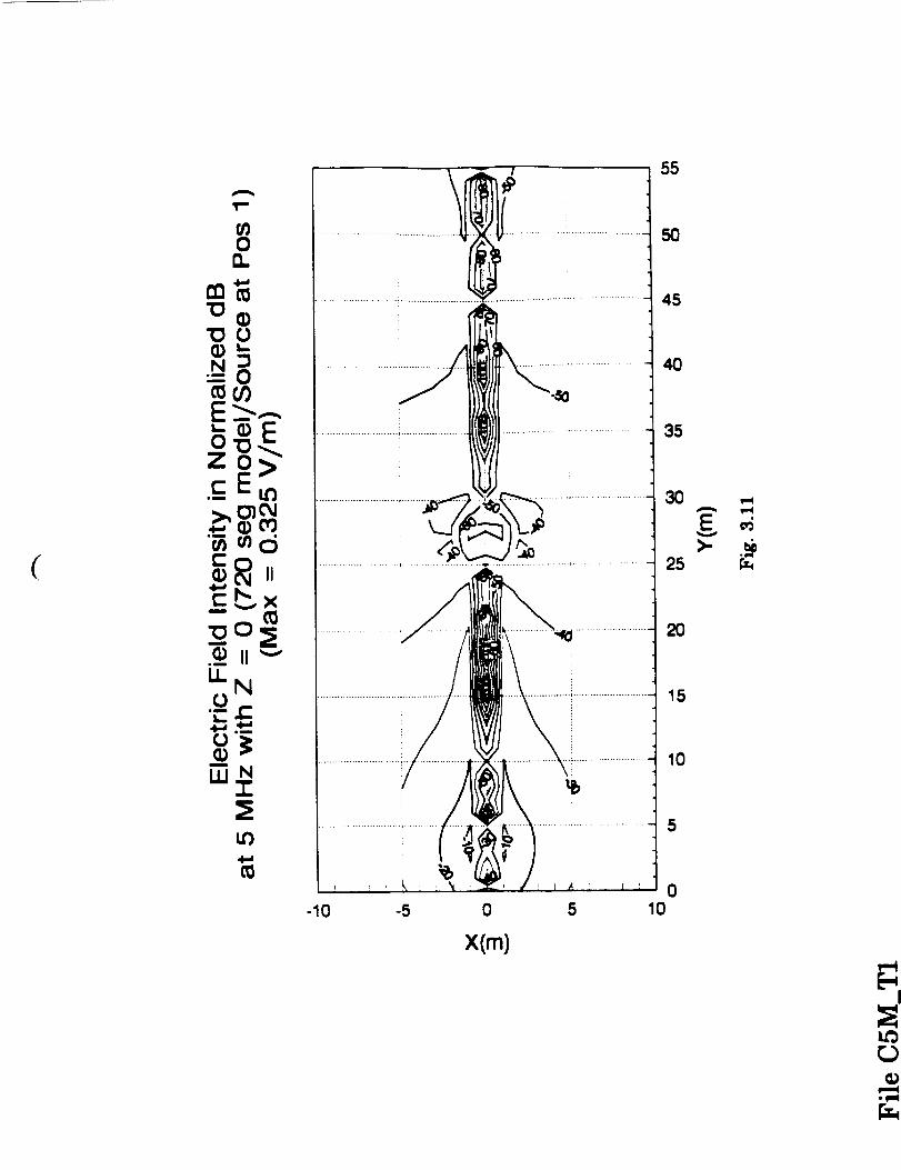
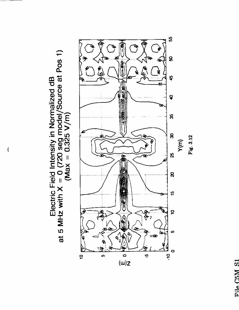
Figure 3.11 File C5M_T1 5 MHzFigure 3.12 File C5M_S1 5 MHz

Figure 3.13 File C20_T1 20 KHz

Figure 3.14 File C20_S1 20 KHz

Figure 3.15 File CSM_T2 5 MHz

Figure 3.16 File C5M_$2 5 MHz


Figure 3.18 File C20_$2 20 KHz

Figure 3.19 File C5M_T3 5 MHz



Figure 3.22 File C20_$3 20 KHz

Figure 3.23 File C5M_T4 5 MHz


Figure 3.25 File C20_T4 20 KHzFigure 3.26 File C20_$4 20 KHz

Top mewSide vmw

Top viewSide wew

Top wewSide wew

Top wewSide wew

Top wewSide wew

Top vlewSide wew

Top wewSide vmw

Top wewSide vmw

Source at location1

Source at location1

Source at location1

Source at location1

Source at location2Source at location2

Source at location2

Source at location2

Source at location3

Source at location3

Source at location3

Source at location3

Source at location4

Source at location4

Source at location4

Source at location4

List of Tables

Table 3.1 Key to Wire-Grid Graphics Files

Appendices

Journal Article: Sheath Wave Propagation in a Magnetoplasma.

II Conference Proceeding: Maguetoplasma Sheath Waves on a Conducting Tether

in the Ionosphere, with Applications to EMI Propagation on Large SpaceStructures.

III Journal Article:A Finite-Element Ballooning Model for2D Eddy Current Open

Boundary Problems forAerospace Applications.

IV Journal Article:The Analysis of the Magnetostatic Fields Surrounding aTwisted-Pair Transmission Line using IntegralMethods.

iv

ANALYSIS OF ELECTROMAGNETIC INTERFERENCE FROM

POWER SYSTEM PROCESSING AND TRANSMISSION


1 Introduction

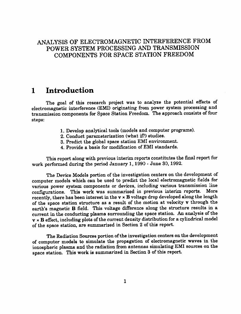
The goal of this research project was to analyze the potential effects of

electromagnetic interference (EMI) originating from power system processing and

transmission components for Space Station Freedom. The approach consists of four

steps:

I. Develop analytical tools (models and computer programs).

2. Conduct parameterization (what if?.)studies.

3. Predict the global space station EMI environment.

4. Provide a basis for modification of EMI standards.

This report along with previous interim reports constitutes the final report for

work performed during the period January 1, 1990 - June 30, 1992.

The Device Models portion of the investigation centers on the development of

computer models which can be used to predict the local electromagnetic fields for

various power system components or devices, including various transmission line

configurations. This work was summarized in previous interim reports. More

recently, there has been interest in the v x B voltage drop developed along the length

of the space station structure as a result of the motion at velocity v through the

earth's magnetic B field. This voltage difference along the structure results in a

current in the conducting plasma surrounding the space station. An analysis of the

v x B effect,including plots of the current density distribution for a cylindrical model

of the space station, are summarized in Section 2 of this report.

The Radiation Sources portion of the investigation centers on the development

of computer models to simulate the propagation of electromagnetic waves in the

ionospheric plasma and the radiation from antennas simulating EMI sources on the

space station. This work is summarized in Section 3 of this report.

1

2. Device Models

1 Introduction

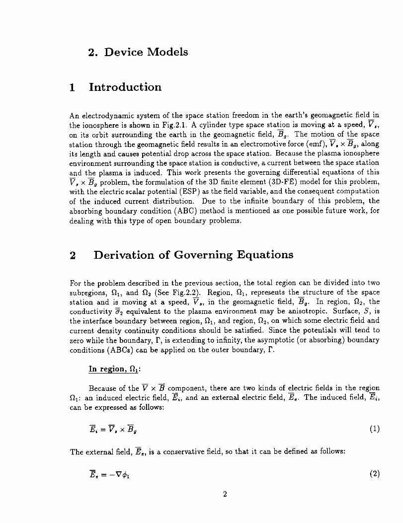
An electrodynamic system of the space station freedom in the earth's geomagnetic field in

the ionosphere is shown in Fig.2.1. A cylinder type space station is moving at a speed, V,,

on its orbit surrounding the earth in the geomagnetic field, Bg. The motion of the space

station through the geomagnetic field results in an electromotive force (enff), V, x Bg, along

its length and causes potential drop across the space station. Because the plasma ionosphere

environment surrounding the space station is conductive, a current between the space station

and the plasma is induced. This work presents the governing differential equations of this

V, x Bg problem, the formulation of the 3D finite element (3D-FE) model for this problem,

with the electric scalar potential (ESP) as the field variable, and the consequent computation

of the induced current distribution. Due to the infinite boundary of this problem, the

absorbing boundary condition (ABC) method is mentioned as one possible future work, for

dealing with this type of open boundary problems.

2 Derivation of Governing Equations

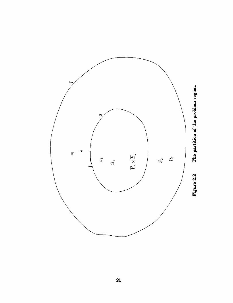
For the problem described in the previous section, the total region can be divided into two

subregions, fll, and f_ (See Fig.2.2_)). Region, _1, represents the_structure of the space

station and is moving at a speed, V,, in the geomagnetic field, Bg. In region, f'/2, the

conductivity 72 equivalent to the plasma environment may be anisotropic. Surface, S, is

the interface boundary between region, fll, and region, _2, on which some electric field and

current density continuity conditions should be satisfied. Since the potentials will tend to

zero while the boundary, F, is extending to infinity, the asymptotic (or absorbing) boundary

conditions (ABCs) can be applied on the outer boundary, F.

In region, ill:

Because of the V x B component, there are two kinds of electric fields in the region

fll: an induced electric field, Ei, and an external electric field, Ee. The induced field, E_,

can be expressed as follows:

E,=V, xBg (1)

The external field, Ee, is a conservative field, so that it can be defined as follows:

Ee = -V¢1 (2)

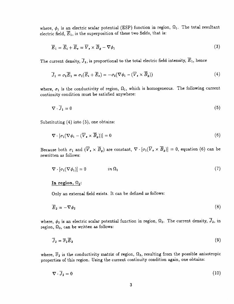
where, ¢1 is an electric scalar potential (ESP) function in region, fh. The total resultantelectric field, 21, is the superpositionof thesetwo fields, that is:

EI=Ei+E,=V, xBg-V¢I

The current density,71, isproportional to the totalelectricfieldintensity,El, hence

(3)

7, = ,:,-,2,= o-_(2,+ 2,) = -o-,(v¢, - (V, x _,)) (4)

where, ch is the conductivity of region, ill, which is homogeneous. The following current

continuity condition must be satisfied anywhere:

v.7, =0 (5)

Substituting (4) into (5), one obtains:

v. [¢,(v¢, - (w, x B_))I = 0 (6)

Because both G, and (V, x Bg) are constant, V. [ch(V, x Bg)] = 0, equation (6) can be

rewritten as follows:

v. [¢,(v¢,)1 =0 i_1 (7)

In region, f_2:

Only an external field exists. It can be defined as follows:

2_ = -v¢2 (8)

where, ¢2 is an electric scalar potential function in region, f_. The current density, J2, in

region, f_2, can be written as follows:

7= = 2,_2a (9)

where, _2 is the conductivity matrix of region, f_a, resulting from the possible anisotropic

properties of this region. Using the current continuity condition again, one obtains:

v.22 =o (10)

3

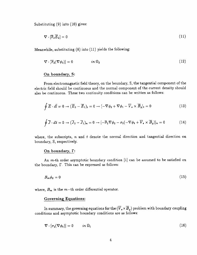
Substituting (9) into (10) gives:

v. [_2] = 0 (11)

Meanwhile, substituting (8) into (11) yields the following:

v. [_2(v¢_)] =o in _2 (12)

On boundary, S:

From electromagnetic field theory, on the boundary, S, the tangential component of the

electric field should be continuous and the normal component of the current density should

also be continuous. These two continuity conditions can be written as follows:

/-E.£=O _ (;2- El), =0 --, [-V¢_ + V¢1-V, x B--_],=0 (13)

J 7. d_ = 0 --, (72 - 71), = 0 _ [-_2V¢_ - _1(-V¢1 + V. x _)], = 0 (14)

where, the subscripts, n and t denote the normal direction and tangential direction on

boundary, S, respectively.

On boundary, F:

An m-th order asymptotic boundary condition [1] can be assumed to be satisfied on

the boundary, F. This can be expressed as follows:

Bm¢2=0 (15)

where, B,,, is the m-th order differential operator.

Governin_ Equations:

In summary, the governing equations for the (V, x Bg) problem with boundary coupling

conditions and asymptotic boundary conditions are as follows:

v. [o_(v¢,)] = 0 in _ (16)

V. [_2(V¢_)] =0 infl2 (17)

(v¢, - v4_), = (v, × B,), on s (18)

(19)

and

B,.¢z = 0 on r (20)

3 Finite Element Formulation

Using the Galerkin-Weighted Residual (CWR) method [2], one can obtain the integral equa-

tions equivalent to the differential equations which were derived in the previous section,

equations (16) through (20). The integral equations can be discretized by finite element

methods [2].

3.1 The Galerkin-Weighted Residual (GWR) method

Using the GWR method, the integral equations can be obtained from the partial differential

equations (16) and (17) as follows:

fn wv. (¢,(V¢,))da = 0 (21)t

wv. (G(v¢z))da = 0 (22)2

where, W is an arbitrary scalar weight function.

From vector calculus, one can write a vector identity as follows:

V . (f F) = fV . F + V f . F ==_ fV . F = V . (f F) - V f . F (23)

where, f is any scalar function and F is any vector function. Let F = gV¢, and f = W,

one can obtain the following useful transformation from (23):

wv. (_v¢) = v. (w(ov¢)) - (vw). (ov¢) (24)

Using the relationship shown in (24), one can rewrite (21) and (22) as follows:

(25)

fo2wv. (v_(v¢2))_=fo2v. (w(_v_2))d_- fo2(vw). (v_v¢_)d_=0 (26)

From vector calculus , Gauss' theorem gives:

f v. _d_ = fs _" d_ (27)

where, fl is a space volume, the closed surface of which is S. The normal direction _ is out

of the volume.

Applying Gauss' theorem, equation (27), to (25) and (26), one can obtain the following:

-/ol (vw). (_v_l)_ + ]s_w(_lv_). _ =0 (2s)

[s,w(_v_). _ + ]_w(_2v_), a_- fo (VW).(_V_)_, =0 (29)

where, $1 = -$2. The second term of the left side in (29) can be dealt with the asymptotic

boundary condition (ABC) method which will be discussed in future work and here assumed

to be zero (the nature boundary condition). That is:

_W(_2V¢_).d_ = 0 (30)

Therefore one can merge equations (28) and (29) into the following:

/o (vw). (_,v¢,)d_+ j(o(vw). (_v¢_)d_ =_, W[_,(v¢_)- _(v¢2)].d_ (31)

6

Substituting the boundary condition (19) into (31) yields:

/o,(vw). + ]o2(vw) (v2v¢2)d = w l(v, ×-&).ds

To simplifying the problem, one introduces some definitions as follows:

(32)

-_ln_ = al; -_In:= _2; (33)

and

¢]n_ = ¢1; ¢ln_ = ¢2 (34)

Using the above definitions, one can rewrite equation (32) as follows:

fn=fllun(VW). (aV¢)dfl = is1 W_a(Vo x -Bg),_ds (35)

3.2 Discretization by FE Method

Define an interpolation function of the scalar potential in a finite element which has m nodes

as follows:

¢'= _ N._¢j (36)j=lt

where, Nj is a shape function, and ej is the potential value at node j. The node numbers of

a given element are 11,12,-.., l,,.

Let us define the weight function in (35) as follows:

W = Ni i = I1, 12,.", l,, (37)

Applying (36) and (37) to (35), one can obtain the element integral function as follows:

l_rtm

Ni¢(V, x Bg),,ds

i = Ii, l_,'",l,_,

(38)

Moving the summation out of the integral, one can rewrite the previous equation as follows:

(39)i, = ll, 12,.", I,,

This relationship can he written in the matrix form as follows:

Sly. ,11 Sl1,12 " " " _11 ,lm

• : : •

Slm,ll 81,n,12 " " " Sire,Ira ¢I.,

hi1

bt_

(40)

Hence, the elemental FE equation can be expressed as follows:

__,.¢_ = b• (41)

where,

s,j = fn (VN,__VN:)da

bi = __f%N,a(V, x Bg),_ds

i,j = ll,12,'",lm

and

(42)

¢e = [¢1_,¢12,'", ¢1_]' (43)

The tangential continuity condition on the interface, S, (V¢1 - V¢2), = (V, x Bg):,

can be considered as a potential jump distribution by which the previous FE formulations

should be modified. In the next section, the potential jump distribution will be discussed.

3.3 FE Formulations Modified by Potential Jump Distribution

On surface, S, we define the potentials as follows:

¢ls = ¢2; (¢2 - ¢1)1s = T (44)

Consider an element, e, which belongs to region, ill, and on interface, S. The total mI e f ! t

nodes on element, e, are 11, 12,..., l,__,, 11, 12,..., l',_,in which ll, 12, •. •, In are on the interface,

8

Se. Meanwhile, the interpolation function in such kind of elements can be expressed as

follows:

I

l,-,.,-_ It,

¢_ = _] N/eli + _] N./¢lj

j=lx j=l' z

(45)

f I I

Because of the fact that ez = ¢2 - T on nodes ll, l:,..., l., the previous equation can be

expressed as follows:

I I I

¢_ = _ N_¢xj + _ Nj(¢2j - T,) = { _ N,¢xj + _ N3¢2,} - _ NjTj

_=_ _=_'_ J=_ J="_ J=_'L(46)

Applying the definition of the potentials in (34) and (44), one can rewrite the previous

equation as follows:

t

1,_ In

¢_= E N,¢j- E NjTj (47)

!

re" = E VN_¢j- E VN_T,j=t_ j=l' t

(48)

For an element which belongs to region, fix, and on surface, S, one can obtain the elemental

equation as follows:I

_-_"[I0. (V Nia-V N_)df_]¢' - i_t, [ln_ (VNiCrV N.)df2]Tj (49)_=l_ =

z[/o(--,-'",)"J+,

or

=/s N,__(V,x -_).dst

i = Ix, 12,'" ", I,,

N.g_(V, x -Bg),,ds + _--_[Lt''' (VN_VN_)dfI]Ti (5o)=_',

i = ll,I2,'",l,,,

Rewriting the modified FE elemental equations in matrix form one obtains the following:

S1 t ,ll 31 t ,12 " " " 8ll ,Ira

: : : :

: : : :

Sire,IX Sl,._,12 " " " Slm,lrn et,,,

bit

bt,,,

(51)

where,

_,, = £ (VN,eVNAdaI

I I I

J = 11,/2,'", I.,(52)

The computation of the potential jump distribution, T, will be presented in the next section.

4 Computation of the Potential Jump Distribution

4.1 Surface Element Analysis

From equation (18), one can see that the potential jump distribution on surface, S, is

governed by the following differential equation:

VT = -(V, x Bg): = -E_t (53)

where, T = (¢2 - ¢1)[s

One can choose a cost functional to be minimized on boundary, S, as follows:

NE.

F(T) = Is [VT + -E_,12ds = _ /s. [VT + E,tl2ds (54)e-=--I

where, NE, is the total number of the surface elements, and S" is the area of a given surface

element. Here we assume that for every element in region, f_l, no more than one element

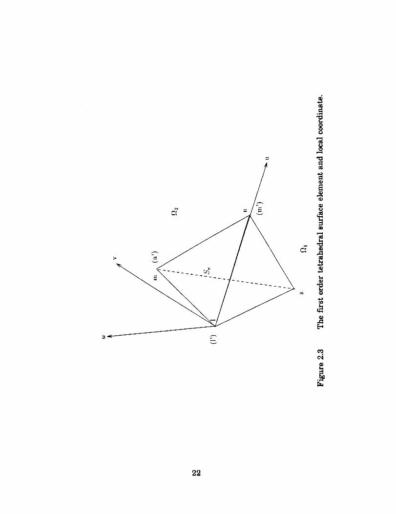
surface is on the surface, S. In this work, first order tetrahedral finite elements are chosen

and only nodes, l',m' and n', can be on surface, S, (see Fig.2.3.).

Define an interpolation function on surface Se as follows:

T: NI, T_, + N,,T,_, + N,,T,, (55)

where, N_,, N,,,, and N., are shape functions on S., and Tl, , T,,,, and T., are the potential

jump distribution on the nodes, I', m' and n'.

A local coordinate system (u, v, w) should be adopted (see Fig.2.3.).

T = T(u, v) = Nt,(u, v)T_, + N,,,,(u, v)T,,,, + N,,,(u, v)T,, (56)

10

Here,

ON,,,,_ ON,,,_+ _'J'.,, +--_-'r=, (57)

aT aNt, _ ON',_ aN.,_ (58)

E_t = E,,_,, + E,,5_ (59)

where, E,, and E,, are constant.

OT^ OT^

V T = -_u a_ + -_v a.

Substituting (59) and (60) into the cost functional, (54), gives:

_'fsC3T OTF(T) = . [(_u a_ + -_-v a_) + (E,,h,, + E_a_)[2dudve=l

= • [(_u + E.)&, + -_v + E")a'12dudve=l

_ NE, [(OT (OT- _ Is. -_u + E,,)' + _v + E.)']dudv

The minimization of the cost functional is as follows:

OF(T) 0 NE. [(c3T OTor, -_ NS. [(07' c30T (c3T 0 OT- _ 2/s. Ou + E")o-_,(-_u)+ -_v + E')-O-f,,(-_v)]dudv

e=l

NE,

,=1 [.OT ON,. (OT _f )]dudv= _2]s (_+E_)(-_-)+ _+Eo)(0

I I I

where, i = l ,m ,n .

Substituting

OF(T)

OT,

(57) and (58)into (62) yields the following:

NS" IS _f_ ON.,,_ ON.,2 [( Tz, + ----_u V', + --_u T=, + E,,)( )e=l

ON t, ON',_ ON,,,_ E_)(_)]dudv+(--_-v T,, + _ T', + ---_--v T=, +

NF,. Is ON, ogt, cON, ON z, c3g, ON', ON, ON',2 [(0u Ou + Ov Ov )T,,+(Ou Ou + Ov Ov )T',e=l

. ON, ON=, c3Ni ON=, ,::3NiE,,+{'Ou Ou + Ov c3v )T=, + _ + E.]dudv = O

(60)

(61)

(62)

(63)

11

where i = l',rn',n'

In the previous equation, all partial derivative terms are constant because of the nature

of the interpolation polynomials in first order elements, so that the elemental equation can

be expressed on S' as follows:

ON, ONe, . ON_ ONe ON, ON,,, ON_ ON.,,

A(--_u -_u - -1- --_v__-_.)T,, + A( -_u --_u_ + O_NOV )T.,,. ONi O-N,, -ONe,ON,, . ONi

+A( _uu Ouu + _-v Ov )7',, = -A(--_-u E,_ + Y-_E_) (64)

i _ Z_T_'_

where, A is the area of the triangular element, e.

The previous equation can be expressed in matrix form as follows:

kt, _, k¢ .¢ k_,., Tz, C¢

k.,, l, k..,,,.,,, k.,,., T.,, = C.,,

k., l, k.,.,, k.,., T., C,.,

where,

ON, ON, ON, ONj.

Ci = -A(-wA E_ + --E,)., , o_4

i,j = I ,m ,n

(65)

(66)

4.2 Local Coordinate System

The local coordinate system (_,, h_, h_,), see Fig.2.3, can be calculated as follows:

_ = u:&= + uy5 u + u,azgem t

llml[

x_'t' &= + Y.,q' ^ + z'_'t--------L'&_Lm't' Lm,l ' ay L"'t,

(67)

or,

Uz

where Y,_'t' =

Zml 1'

l[x 1Lm,t ' Ym't'Z"`' i'

Xml -- Xl_ ]

- v,,] = + +Y,,¢

Z m, -- Zll

(68)

&w = w=a= + wyay + w,h, -(l'm' x l'n') 1

ll'm' x l'n'[ 2&

a= ay 5,

X"`ll' Ym't' Zrnll I

xn'l' YnT ZnT

(69)

12

or,

where,

[wx]Wy

Wz

F

1 ] Yrn'l'Znq' -- Yn'l'Zm'l'

2A [ Xn'l'Zm'l' -- Xm'l'Zn'l'Xmtl'yn' l' Xn'l'Ymll j

..is] ]Y.'l' = Y : -- Yl'

Zn'l t Zn' -- Zlr

and A is the area of the triangle l'm'n' on surface S':

(70)

or,

= v_a_ + vyay + v.a. = a,. x 5_,

- 2AL,,t, Ym'_'z,'¢ - y,,l,z,_,t,Xm'lJ

&u &z

Xn, l, Zrn,l _ -- Xm,l, Zn, l j Xrn'l'Yn'l _ -- Xn,lJYm, l,

Ym' l_ Zrn' l'

V x

Yy

_z2AL,,,,¢

(72)

(73)

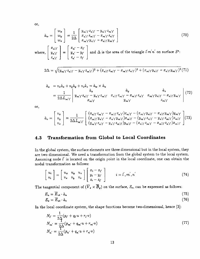
4.3 Transformation from Global to Local Coordinates

In the global system, the surface elements are three dimensional but in the local system, they

are two dimensional. We need a transformation from the global system to the local system.

Assuming node l' is located on the origin point in the local coordinate, one can obtain the

nodal transformation as follows:

U i U x Uy U z , , ,

v, = v_ % v_ Y,-YI' i=l,m,n (74)Z i -- Z/,

The tangentialcomponent of (V, × Bg) on the surface,S,, can be expressed as follows:

S. = E_t" _. (75)

E,, = ;_t" a,, (76)

In the local coordinate system, the shape functions become two-dimensional, hence [3]:

N t, = 2_(P¢ + ql'u + rl,v)J

Y.., = 2-=K (;.., + + (77)

N,¢ = 2A (p"' + q.,u + r.,v)

13

and

where

ONt__:= ql' OWl, r__2,"

00/_., 2_; 0_m,-2A'__ qm . rmt

0 , _ q.,. 0 , r.,

Ou - 2A' Ov 2A

pll = Um_Vn* --UnfVm_; ql t = Vm* -- yn_i?¥ = Un_ --Urn_

Pro' = Un_Vl' -- Ut'Vn'; qm _ = Vn' -- Vl';rm' = Ul_ -- Un'

Pn' = Ul'Vm' -- Um'VI'; qn' = V|' -- Vm'; rn_ = Um_ -- U l'

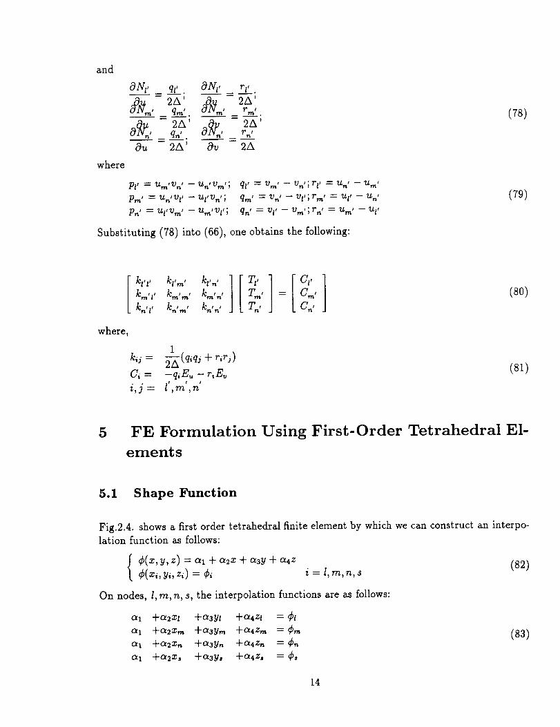
Substituting (78) into (66). one obtains the following:

(78)

(79)

[k 1[c]kin, l, k.¢.¢ k..,., T,_, = C._,

k., z, k.,._, k.,., T., C.,

where,

1

kij - 2A(qiqj + fir1)

Ci = - qiE_, - riE_

l .m .ni.j= ' ' '

(so)

(81)

5 FE Formulation Using First-Order Tetrahedral El-

ements

5.1 Shape Function

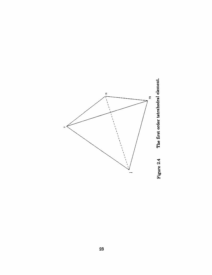
Fig.2.4. shows a first order tetrahedral finite element by which we can construct an interpo-

lation function as follows:

¢(x.y.z) -- o_1 -_ o_2x + aaY -[- o_4z (82)¢(xi, yi, zi) = ¢i i = l, m, n, s

On nodes, l, m, n, s, the interpolation functions are as follows:

al "_-(22Xl "_(23YI "_Ot4Zl = ¢1

O_1 "_-C_2Xm -_-c_3Yrn AYOt4Zm = Cm

al +a2Xn +aay,_ +a4zn = ¢,,

al +a2xs +a3y, +a4z, = ¢.

(83)

14

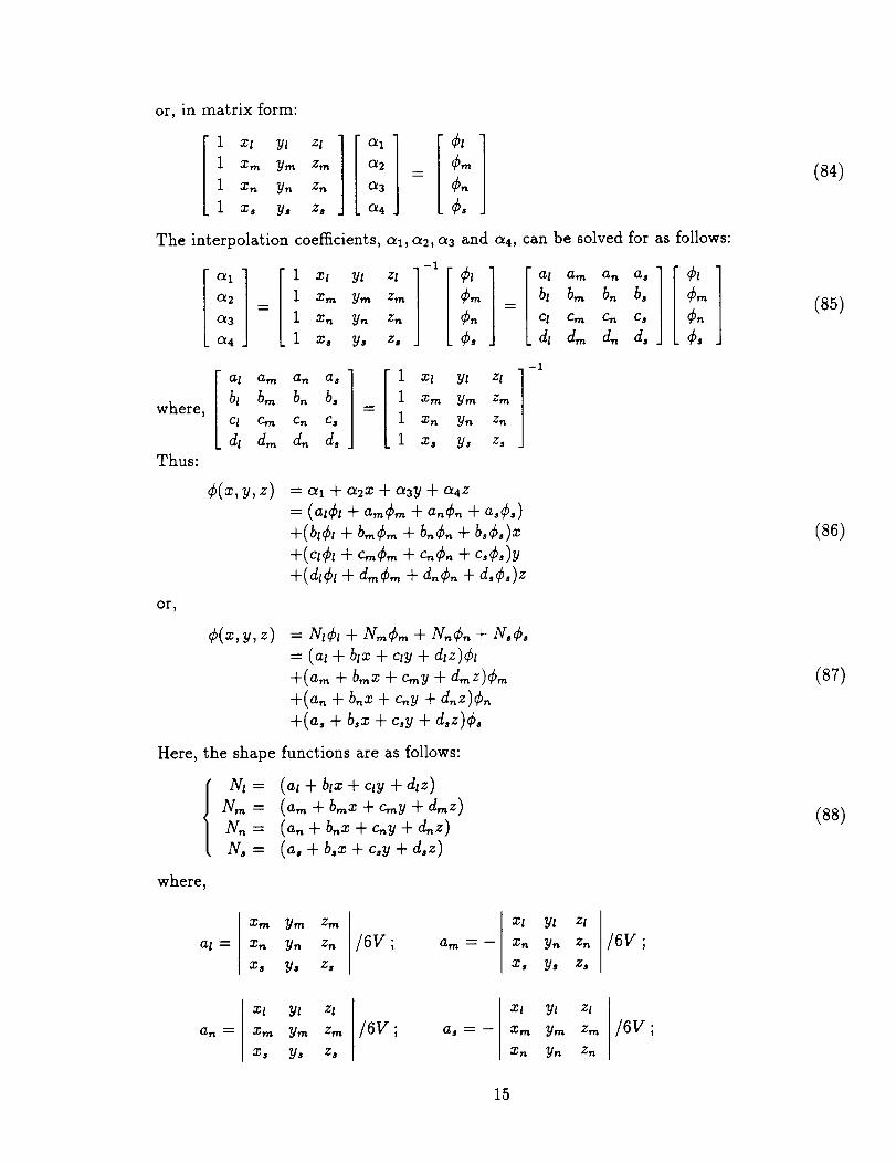
or, in matrix form:

1 xl Yl zl

1 Xm ym Zm

1 X,_ y. Z.

[ Xs Ya Zs

The interpolation

ot 2

ot 3

o_4

al am

bt bmwhere,

cl cm

d_ d.,Thus:

¢(x,y,z)

or,

¢(x,y, Z)

ct I

ot 2

ot 3

a4

---- Cm¢.Cs

coefficients, al, a2, a3 and a4, can be solved for as follows:

1 xt Yt zt

l xrn Yrn Zm

1 Xn Yn Zn

1 Xs Ys Zj

1

1

1

1

-1

xl Yl

Xm Ym

xn Yn

Xs Ys

an as

b,_ b.

Cn Cs

dn d,

-1zl

zm

Zn

Z$

= al + a2x + a3y + a4z

= (at¢l + amCm + an¢. + as¢.)

+(bl¢_ + bmCm + b,.¢,, + bs¢.)x

+(c,¢t + cm¢_+ c.¢. + cs¢s)y+(diet + d._¢,,, + dn¢. + ds¢s)z

= N_¢_ + N,_¢,_ + Nn¢,, + Ns¢s

= (at + blx + cry + dlz)¢t

+(a._ + bmx + c_y + d,_z)¢m

+(a. + b,_x + c,_y + dnz)¢,.

+(as + b,x + csy + dsz)¢s

Here, the shape functions are as follows:

(at + blx + cry + dtz)

(a,_ + bmx + c_y + dmz)

(a,, + b,,z + c,,y + d,,z)

(a, + b,x + c,y + d,z)

at am an as

bl bm b. b.

Cl Cm Cn Cs

dt dm d. d,

_t

¢.¢.

where,

Nl=

Nm

N.N,

al =

xm Ym

Xn Yn

Xs Ys

Zm

z. /6V;Zs

a m _ _

xt Yt

xr, yn

Xs Ys

Zl

z., /6V ;Zs

(84)

(85)

(86)

(87)

(88)

a n

xt Yl

xm Ym

xs Ys

zt

z,., /6V ;Zs

a s _ _

xt Yt

xm yra

xn y,_

Zl

z., /6V ;Zn

15

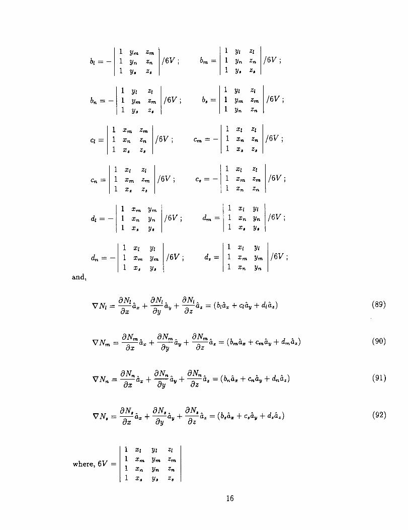
b I _ _

i y._

1 y.

i y,

Zm

z. /6V ;Zs

bErL

1 Yt

i y.

i y,

zl

z. /6V ;Zs

i y_

i y,_

1 Yo

zl

z,. /6V ;Zs

b o -_-

i Yl

1 y,.,

1 y.

zl

z., /6V ;Zn

1 X m

i x.

i x,

Zm

z. /6V ;Zo

1 xt

1 x.

1 x,

z!

z. /6V ;Zo

Cn

1 x!

I xm

i xs

zl

z._ /6V ;Zs

Co _ m

1 xl

1 xm

1 Xn

Z!

z., /6V ;Zn

d! _ m

1 Xm

1 x.

1 x,

Y_

y. /6V ;

y,

dm _"

1 xl

i x.

yl

y. /6v ;Y,

and,

dn _- --

1 xl

i xm

i xo

Yl

y., /6V ;Y.

do

1 xt

1 xm

1 x.

Yl

y,,, /6v ;Y.

ON! ^ ONl^ ON!^ = (bla_ + clay + dial)VNt = a----_a:_+ a--_-% + a----_a.

(89)

_T Y m _ ON,,, ON,_^ ONto^ = (b._a:: + c_&u + din&.)a= &=+ O---y-aw-F 0--'7 a"

(90)

VN.- aN,, aN.^ ON,,^ (b,,&= + + d.&.)- + a-T%+ -Ea, = (91)

VN,- OY,. aN,. ago^ = (boa. + c,a, + doa,)- a----[_x+ a---_%+ a--_,

(92)

where, 6V =

1 xl y! zl

1 xm Ym zm

1 x. y. z.

1 xo Y. z,

16

5.2 FE Formulation

Using the first order tetrahedral element, one can discretize elemental equation, (52), as

follows:

J,r {a ON'ONj ON, ONj ON, ONj&j

= (cr=b, bj + ayclcj + a.d, dJ. V

b, = al(V, × -Ba),_ Is g, ds + Si._' Tj'j' =l' ,ra _,n _,s _

= ol(V, × -Bg)./x_----_"3 + Y]_ Si'3'T"I I t I I

2 -'_ ,rn ,n ,$

i,j = l,m,n,s

(93)

where, At,_,_ is the area of the triangle (nodes I, m, n); subscript, n denotes the normal direc-

tion on surface S[; symbol, j' is the node on surface S[; V is the volume of the tetrahedral

element, e.

6 Calculation of Current Density

The current density is proportional to the electric field intensity.

In region, fh:

71= o-12,= 0-,(2,+ 2,) = -o-,(v¢, - (V, x _9)) (94)

where, or1 is the conductivity of region, f_l, which is homogeneous.

From (47) and (48), the element potential and its gradient can be expressed as follows:

I._ l,_

._=l, .7=_[

(95)

t

re" : _ VY3¢,- _ VN_Z, I

j=ll :=I_

(96)

17

The element current density can therefore be calculated by:

!

(97)

where, VN, (i = l,m,n,s) can be calculated using equations (89) through (92).

In region, f_2:

In this region, no (V x B) component and no potential jump are encountered. Hence,

the current density of the element becomes:

= -v2 "(E vY,¢A (98)J=h

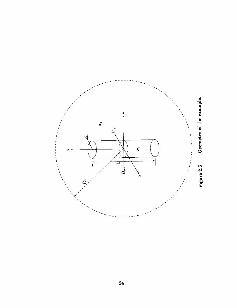
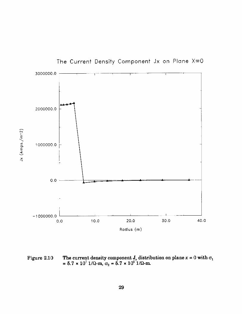
7 Example

In this work, an example (see Fig.2.5) is chosen to verify that the practicality and utility

of the 3D-FE model developed in the previous sections. In Fig.2.5, we choose a cylinder as

the moving object in place of the space station. Some geometric parameters and physical

parameters are as follows:

the length of the cylinder, L = 20 m

the radius of the cylinder, R = 5 m

the radius of the outer sphere boundary, R0 = 40 m

the flux density along the negative z-axis, Bg = 0.45G = 0.45 x lO-4Wb/m 2

the speed of the cylinder along the negative y-axis, V_ = 8km/sec.

the conductivity inside the cylinder, al = 5.7 x 10 r 1/(fl • m)

the conductivity outside the cylinder, a2 = 5.7 x 105 1/(fl • m)

The outer boundary condition in this example is assumed to be the natural boundary con-

dition.

The 3D-FE gird with a total number of elements, NE=3456, and a total number of

nodes, NN=669, is shown in Fig.2.6. An FE grid with a total number of elements, NE=28128,

and a total number of nodes, NN=4963, is chosen for the FE computation, whose surface

elements on the cylinder and outer boundary are shown in Fig.2.7. The equipotential lines

and the current density distribution along the plane of the cross section (z = 0, y > 0) were

plotted from the results of this FE model see Fig.2.8 and Fig.2.9, respectively. The numerical

results of the current density component J= vs radius on Plane x=0 are plotted in Fig.2.10.

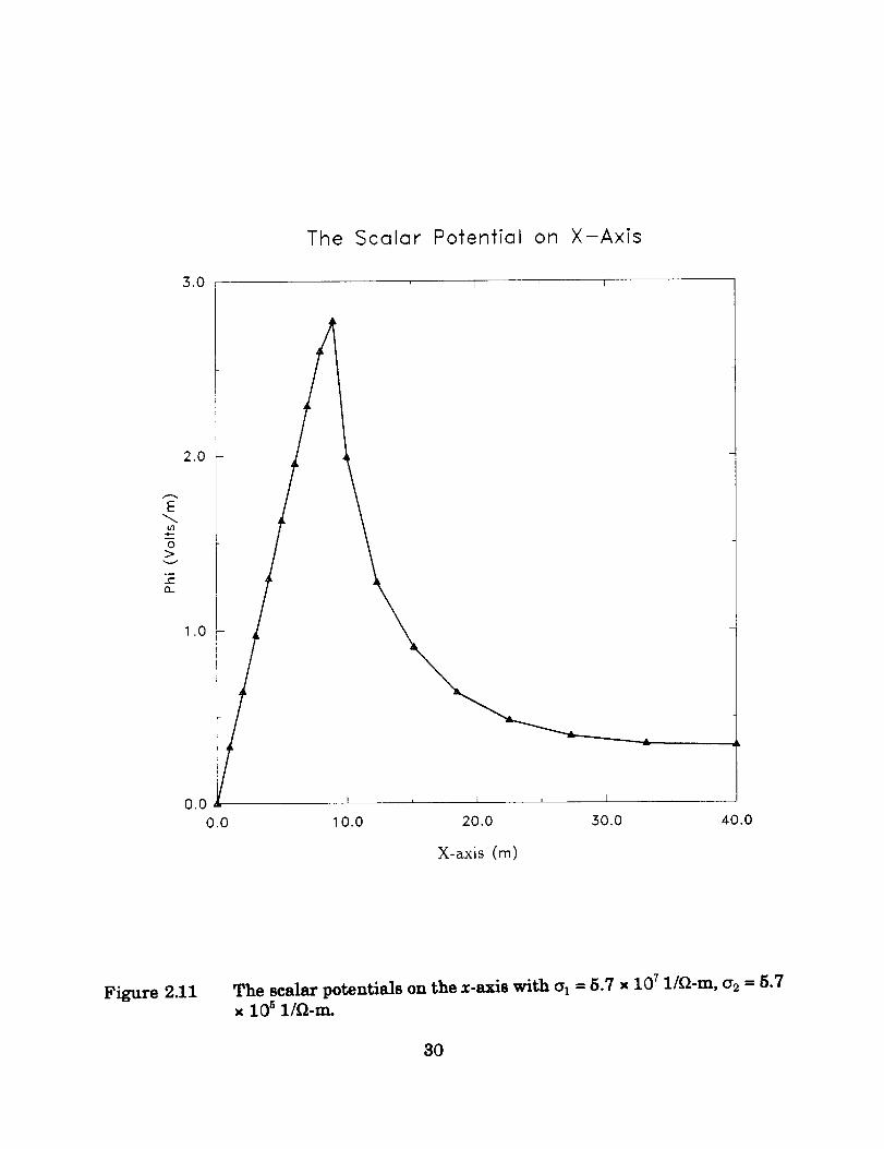
The numerical results of the scalar potentials located on the x-axis are plotted in Fig.2.11.

18

8 Conclusions and Possible Future Work

As a result of this investigation two technical papers on ballooning FE models and on twisted-

pair transmission lines were presented at the IEEE INTERMAG-92 Conference, and were

simultaneously published in the September issue on the IEEE Transactions on Magnetics

(IEEE Trans. on Magn. Vol.30, No.5, 1992). These papers are included here in Appendix

(III) and Appendix (IV), respectively.

Meanwhile, in order to obtain higher accuracy results regarding the present (V, x Bg)

problem formulated in this report, the asymptotic boundary conditions (ABCs) should be

adopted instead of the natural boundary conditions. High order ABCs can improve the

accuracy of the numerical results.

When the moving body is long and slender, a sphere shape outer boundary would

be "storage memory intensive" and numerically inefficient. It would be highly desirable

to choose an outer boundary that is conformal to the shape of the object. A formulation

based on the ABCs should be derived for this 3D-FE scalar potential problem with an outer

boundary of an arbitrary shape ( an ellipsoid is one possibility).

In future work, the flux density distribution caused by the resulting pattern of induced

current in the plasma and structure can be computed. This can be accomplished by a 3D-

FE vector potential formulation using second order elements with the ABCs on the outer

boundary, which should be designed to accommodate various shapes of the orbiting body

under consideration.

References

[1] R. Mittra "Review of Absorbing Boundary Condition for Two and Three-Dimensional

Electromagnetic Scattering Problems" IEEE Trans. on Magn., Vol.25, No.4, July, 1989, pp

3034-3039

[2]Zienkiewicz and Talor The Finite Element Method, McGraw-Hill Book Company

(UK) 1989

[3] S. Ratnajeevan H. Hoole Computer-Aided Analysis and Design of Electromagnetic

Devices, Elsevier Science Publishing Co., Inc. 1989

19

_Dc_

0

_DaD

°l-i

r_

o

Cr_

_S 1.1

o o

0_

C_

20

0

tml

_o

o

o

p_

21

c_

"0

00

8

lID

III

rll 0

r_

22

E _

I.i0

a

_4c4

23

f \

/ \

// \

24

X._

1"4

0

U II

• LO

_I It

25

X_

c_P_

0..Q

c_

aoa_

I.i

_S

P_S

aD

L_.

I.i

r_

26

m

t

/

/

/

N

/

/

\

0

AI

II

0

oM

0

.p,l

o

,I..4

C,1

27

II

/

/

/

/

/

/

/

.. -.._...:.__,,,,,.-,-.--:._• ........-:--,,

-\

\

\

\)-

0

0

0

_0

0

O_

28

The

3000000.0

Current Density Component Jx on

I I I

Plane X=O

c',4

e-

E

,4{D..

E

v

x

2000000.0

1000000.0

O.O

-1000000.0

O.O

_, __ J. J. A

L I , I L I ,

10.0 20.0 30.0 40.0

Radius (m)

Figure 2.10 The current density component '-Ixdistribution on plane x = 0 with al

= 5.7 x 107 l/_-m, a2 = 5.7 x 105 l/_-m.

29

The Scalar Potential on X-Axis

3.0 I I I

E

0

L213-

10.0 20.0 30.0 40.0

X-axis (m)

Figure 2.11 The scalar potentials on the x-axis with ol = 5.7 x 10 7 1/f_-m, o2 - 5.7

x 10 5 l/f_-m.

3O

3 Radiation Sources

This portion of the investigation centers on the development of computermodels to calculate the radiation from simulated electromagnetic interference (EMI)

sources on the space station.Section 3.1 briefly describes the plasma environment of the ionosphere within

the altitude range corresponding to the orbit of the space station. It is shown thatthe anticipated frequencies of potential EMI sources fall weU below the plasmafrequency. Therefore, radiation at these frequencies will be attenuated by the

plasma. Method-of-moments analyses of the radiation by sources on a straight wireand on a simple model of the space station demonstrate that both the currents in thestructure and the electric fields around the structure may be calculated. Calculated

results are also shown for the simple model of the space station embedded in a zero-

order-plasma. This plasma approximation includes the charged particle density atthe altitudes of interest, but neglects the geomagnetic field, thereby resulting in an

isotropic rather than an anisotropic plasma. The results show that while the plasmaattenuates the radiation, induced currents in the structure nevertheless produceradiated fields that exceed those that would be present in the absence of the

conducting space station structure. Software that can be used to visualize contour

diagrams of the calculated electric field distribution around the simple model of thespace station is described.

Section 3.2 describes the development of a wire-grid model of the space stationthat has been analyzed using the method-of-moments by the ElectromagneticEnvironmental Effects Laboratory at the Georgia Tech Research Institute. This isalmost the same approach that the European Space Agency is using to predict EMI

problems on their spacecraft. Calculations have been made for eight different casescomprising two source locations, two polarizations, and two frequencies, 20 KHz and5 MHz. The calculated results show top view and side view contour graphs of the

electric field for each case - a total of sixteen graphs. Software that can be used tovisualize both the wire-grid space station model and contour diagrams of thecalculated electric field distribution around the space station is described.

Section 3.3 briefly summarizes the available literature on plasma sheathwaves. Excerpts from three recent publications, a journal article and two conference

proceedings, are given. It has been shown (by others) that a region of low chargedensity, called a sheath, forms around a conducting object, like the space station,when it is embedded in the ionospheric plasma. A source on the conducting object

can very efficiently transfer electromagnetic fields to distant locations by launchingwaves in the sheath region. The condition for transmission is the opposite of that for

propagation in the ambient plasma as described in Section 3.1. Namely, sheathtransmission is unattenuated for frequencies below the plasma frequency and is

attenuated for frequencies above the plasma frequency. Sheath waves may therefore

be an important factor in EMI analysis.Section 3.4 briefly summarizes the available literature on finite-difference time-

domain analyses of electromagnetic wave propagation in anisotropic plasmas. The

31

abstracts of three publications, two journal articles and a conference proceeding, are

given. These new analysis tools may be important for predicting the propagation of

EMI signals in realisticmodels of the ionospheric plasma, i.e.,a plasma model that

includes both the charged particles and the geomagnetic field.

3.1 Simple Wire Model of Space Station Freedom in a Zero-order Plasma

The space station will be embedded in the ionospheric plasma, a region of

dense electriccharge. As far as electromagnetic wave propagation in the ionosphere

is concerned, the ionosphere can be modelled as an isotropic plasma if the

geomagnetic field is neglected. Electromagnetic waves are then attenuated when

their frequency is below the plasma frequency, but they propagate freely and

unattenuated when their frequency isabove the plasma frequency. Most importantly,

the direction in which the wave istraveling is immaterial -exactly the same behavior

occurs. However, when the geomagnetic field is considered, the plasma becomes

anisotropic and the affect of the ionosphere on electromagnetic wave behavior

depends on the direction of the electromagnetic wave relative to the direction of the

magnetic field. All electromagnetic interference analyses to date have assumed an

isotropic plasma, i.e.,the geomagnetic field has been neglected. This assumption

seems appropriate when what is needed is the basic behavior of electromagnetic

interference in the presence of the plasma - to assume otherwise would greatly

complicate any numerical calculations with littleimprovement in understanding the

basic behavior of the interaction.

The key parameter in studying electromagnetic wave propagation in a plasma

is the plasma frequency

I Ne 2 (i)(Dp - -- ,meeo

where N is the electron density in electrons per m 3, e is the electron charge in

Coulombs, m e is the electron mass in kg, and _ is the permittivity of free space.

Although the ionosphere consists of both electrons and ions, most of the interaction

occurs with the electrons because they have a much smaller mass, and therefore are

more responsive to the influence of electricand magnetic fields. That is the reason

that the plasma frequency is written only in terms of the electron charge and mass.

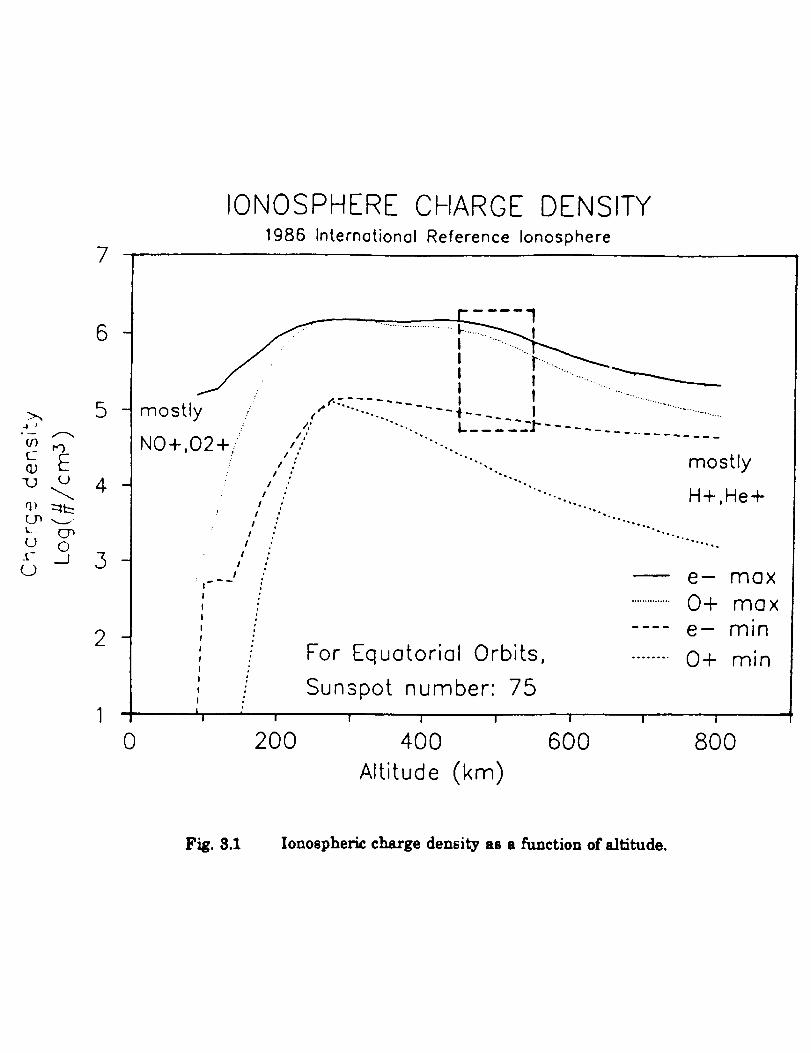
The variable factor in eq. (1) is the electron density N. Figure 3.1 shows the

ionospheric charge density as a function of altitude for an equatorial orbit

corresponding to the orbit of the space station. If only the electrons are considered,

and an orbit altitude of 450 to 550 kilometers is assumed, itcan be seen that logioN

fallsin the range of 4.7 to 6.3 as shown in the outlined rectangular region in Fig. 3.1.

This corresponds to an electron density N of 0.05 x 1012 to 2.0 x 10 n electrons per m 3.

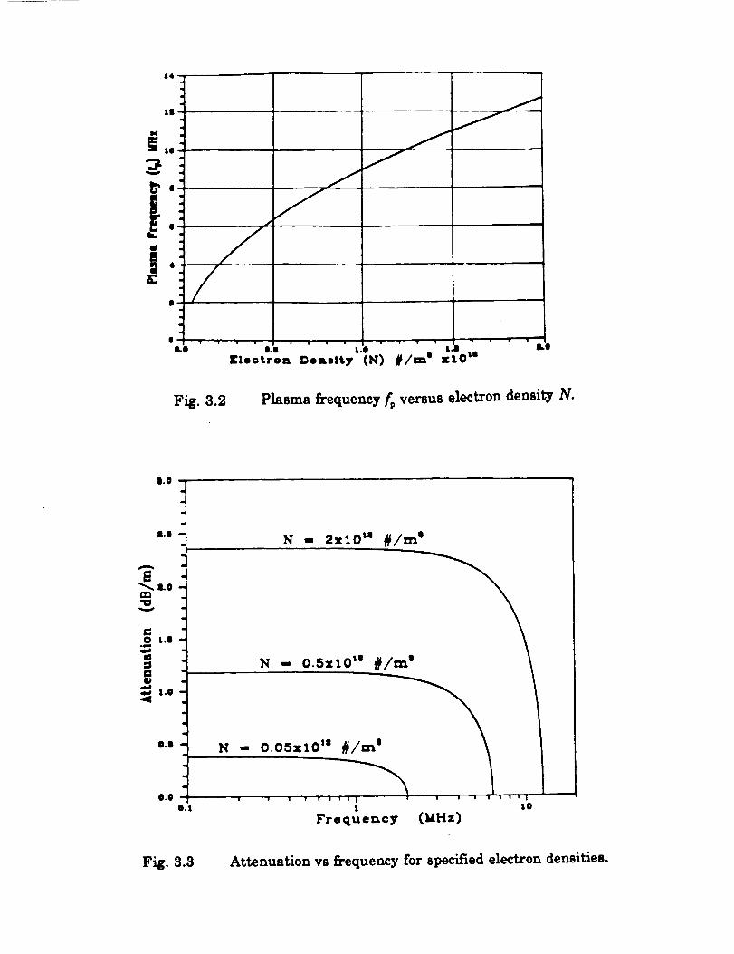
Figure 3.2 shows the calculated plasma frequency, fp = 2_cop,for the assumed

range of N. From the graph, itcan be seen that the minimum plasma frequency of

32

2 Mhz corresponds to the minimum electron density. Since propagation occurs for

frequencies above the plasma frequency and attenuation occurs for frequencies below

the plasma frequency, attenuation is expected for all frequencies below 2 Mhz. A

plane wave is attenuated by a factor of exp(-ar), where a is the attenuation factor in

m" and r is the distance in m. The attenuation factor a is dependent upon the

frequency of propagation co relative to the plasma frequency cop according to

-1(2)

Figure 3.3 shows the calculated attenuation in dB/m as a function of frequency for

different electron densities. The attenuation factor increases with increasing electron

density. For a given electron density, the attenuation is fairlyconstant until the

plasma frequency is approached, at which point the attenuation drops to zero

according to eq. (2).

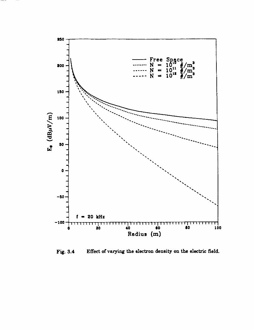
The effect of the plasma on electromagnetic wave propagation is explicitly

shown in Fig. 3.4. This shows the 0 - component of the electricfield radiated by a

short dipole as a function of distance away from the dipole for free space (zero

electron density) and for electron densities from 0.01 x 10 x2to 1.0 x 1012 per m 3. It

is clear that increased electron density results in increased attenuation. Here we

have assumed that the near-field attenuation of the dipole fieldsoccurs in a similar

way as far-fieldattenuation.

The above has considered the effects of the plasma on electromagnetic wave

propagation, but without the presence of the space station structure. The influence

of physical structure can be incorporated by using the method of moments, a well-

known numerical electromagnetic analysis method. The method of moments can be

used to find the currents and the local electromagnetic fields about a conducting

structure which has been excited by a current or voltage source. The calculation

finds both the currents and the fields. In fact,the solution procedure fn'stfinds the

currents and then calculates the fields radiated by these currents. As an example,

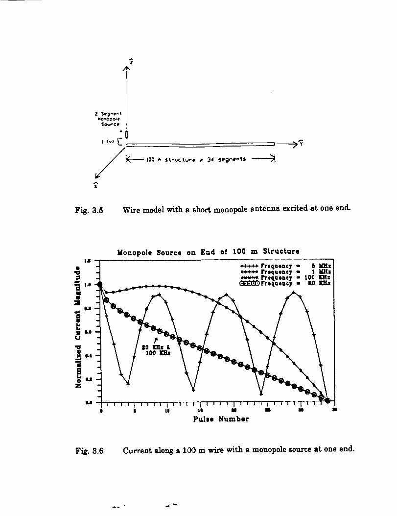
Figure 3.5 shows a 100 m wire (divided into 34 segments for analysis) excited by a

short monopole antenna at the lei_end. The current distribution in the wire is then

calculated for a 20 KHz, 100 KHz, 1 MHz, and 5 MHz source for the free-space (no

plasma) case. The calculated current distribution is shown in Fig. 3.6. At the lower

frequencies of 20 and 100 KHz, the normalized current distribution isthe same. The

smooth decrease of the current from the maximum at the source end to zero at the

far end is characteristic of an antenna that is short relative to a wavelength. The

wavelength at 100 KHz is 3000 m, so the structure is about 0.033 wavelengths in

length at this frequency. The length of the wire in terms of wavelengths is even

shorter at 20 KHz. As the frequency increases to I MHz, the distribution changes

only slightly,as the structure is now about 0.3 wavelengths in length. However, at

5 MHz, the structure is 1.67 wavelengths in length. Since we expect standing waves

33

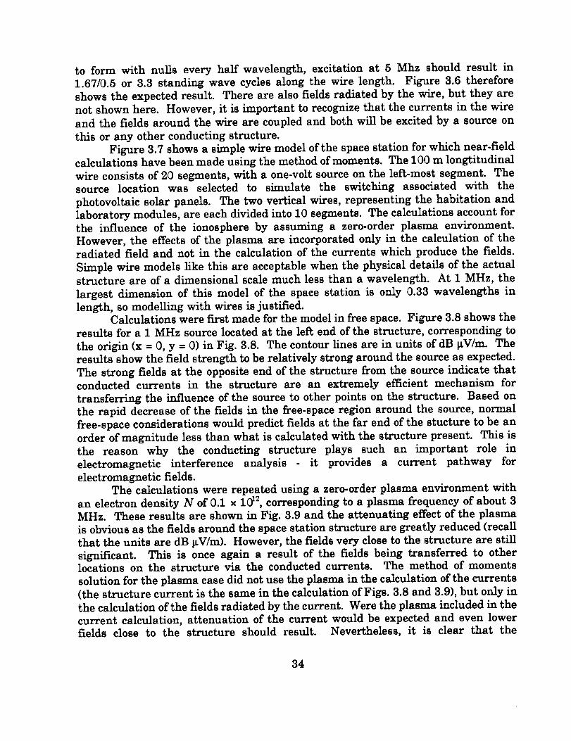
to form with nulls every half wavelength, excitation at 5 Mhz should result in1.67/0.5 or 3.3 standing wave cycles along the wire length. Figure 3.6 thereforeshows the expected result. There are also fields radiated by the wire, but they arenot shown here. However, it is important to recognize that the currents in the wireand the fields around the wire are coupled and both will be excited by a source on

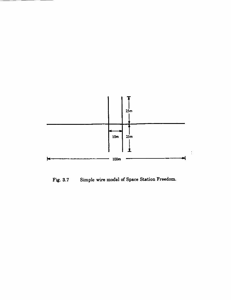
this or any other conducting structure.Figure 3.7 shows a simple wire model of the space station for which near-field

calculations have been made using the method of moments. The 100 m longtitudinal

wire consists of 20 segments, with a one-volt source on the left-most segment. Thesource location was selected to simulate the switching associated with the

photovoltaic solar panels. The two vertical wires, representing the habitation andlaboratory modules, are each divided into 10 segments. The calculations account forthe influence of the ionosphere by assuming a zero-order plasma environment.

However, the effects of the plasma are incorporated only in the calculation of theradiated field and not in the calculation of the currents which produce the fields.

Simple wire models like this are acceptable when the physical details of the actualstructure are of a dimensional scale much less than a wavelength. At 1 MHz, the

largest dimension of this model of the space station is only (}.33 wavelengths in

length, so modelling with wires is justified.Calculations were first made for the model in free space. Figure 3.8 shows the

results for a 1 MHz source located at the left end of the structure, corresponding to

the origin (x = (}, y = 0) in Fig. 3.8. The contour lines are in units of dB _V/m. The

results show the field strength to be relatively strong around the source as expected.

The strong fields at the opposite end of the structure from the source indicate thatconducted currents in the structure are an extremely efficient mechanism for

transferring the influence of the source to other points on the structure. Based on

the rapid decrease of the fields in the free-space region around the source, normal

free-space considerations would predict fields at the far end of the stucture to be an

order of magnitude less than what is calculated with the structure present. This is

the reason why the conducting structure plays such an important role in

electromagnetic interference analysis it provides a current pathway for

electromagnetic fields.The calculations were repeated using a zero-order plasma environment with

an electron density N of (}.1 x 10:2, corresponding to a plasma frequency of about 3MHz. These results are shown in Fig. 3.9 and the attenuating effect of the plasmais obvious as the fields around the space station structure are greatly reduced (recall

that the units are dB IzV/m). However, the fields very close to the structure are stillsignificant. This is once again a result of the fields being transferred to otherlocations on the structure via the conducted currents. The method of moments

solution for the plasma case did not use the plasma in the calculation of the currents(the structure current is the same in the calculation of Figs. 3.8 and 3.9), but only inthe calculation of the fields radiated by the current. Were the plasma included in thecurrent calculation, attenuation of the current would be expected and even lowerfields close to the structure should result. Nevertheless, it is clear that the

34

conducting structure plays a significant role in producing fields close to the structurethat are substantially greater than would be expected from consideration of radiationeffects alone.

Computer Visualization

The calculated method-of-moments results in Figs. 3.8 and 3.9 may be viewed

on a color monitor. An IBM-compatible PC with 512 Kb memory and (preferably) a

hard disk is required. A graphics program called TOPO, licensed from Golden

Software, Inc., may be used.First create a directory on the hard disk called TOPO and change to this

directory. Then insert Disk #1 into the 3.5" floppy disk drive, switch to the floppy

disk drive, change to directory TOPO, and copy all fries to the hard disk (usually

drive C:). Then switch back to the hard disk. The contour graphs may be generated

as follows:

type topo/cmd=fs (upper or lower case)

when the program is loaded, press F2 to display Fig. 3.8 (free-spaceresult)

press ESC when finished viewing

press ESC and RETURN to exit the graphics program

repeat the above except type topo/cmd=zop to display Fig. 3.9 (zero-orderplasma result)

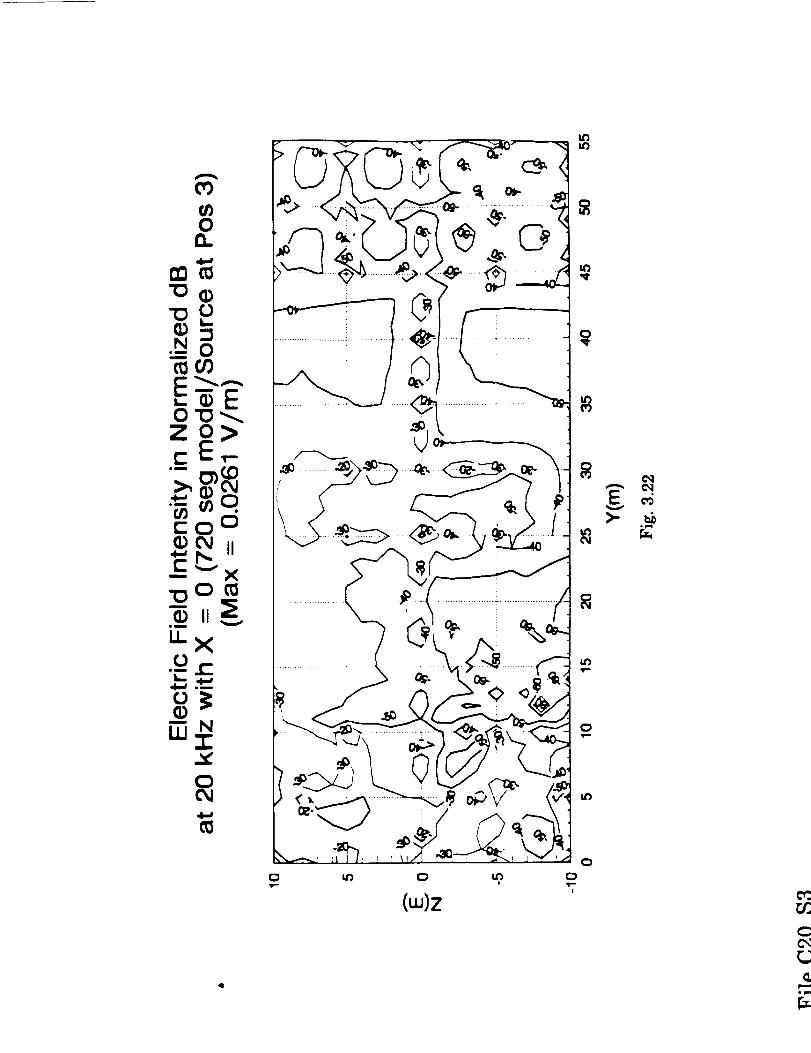
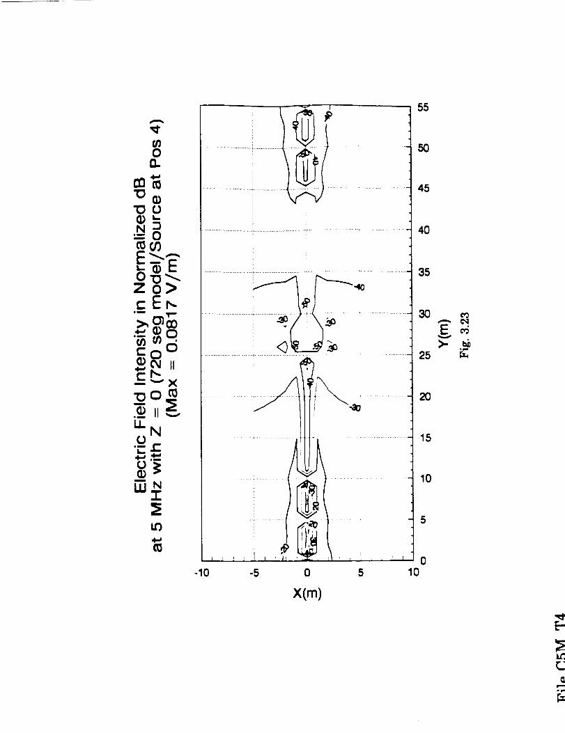
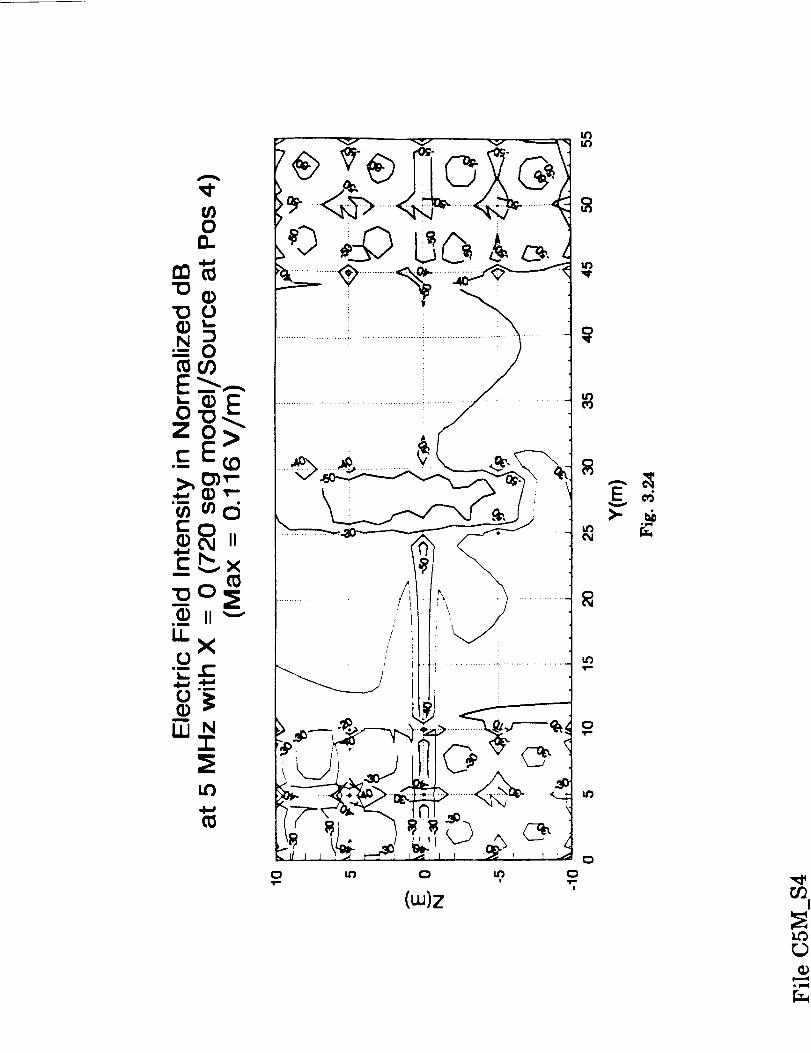
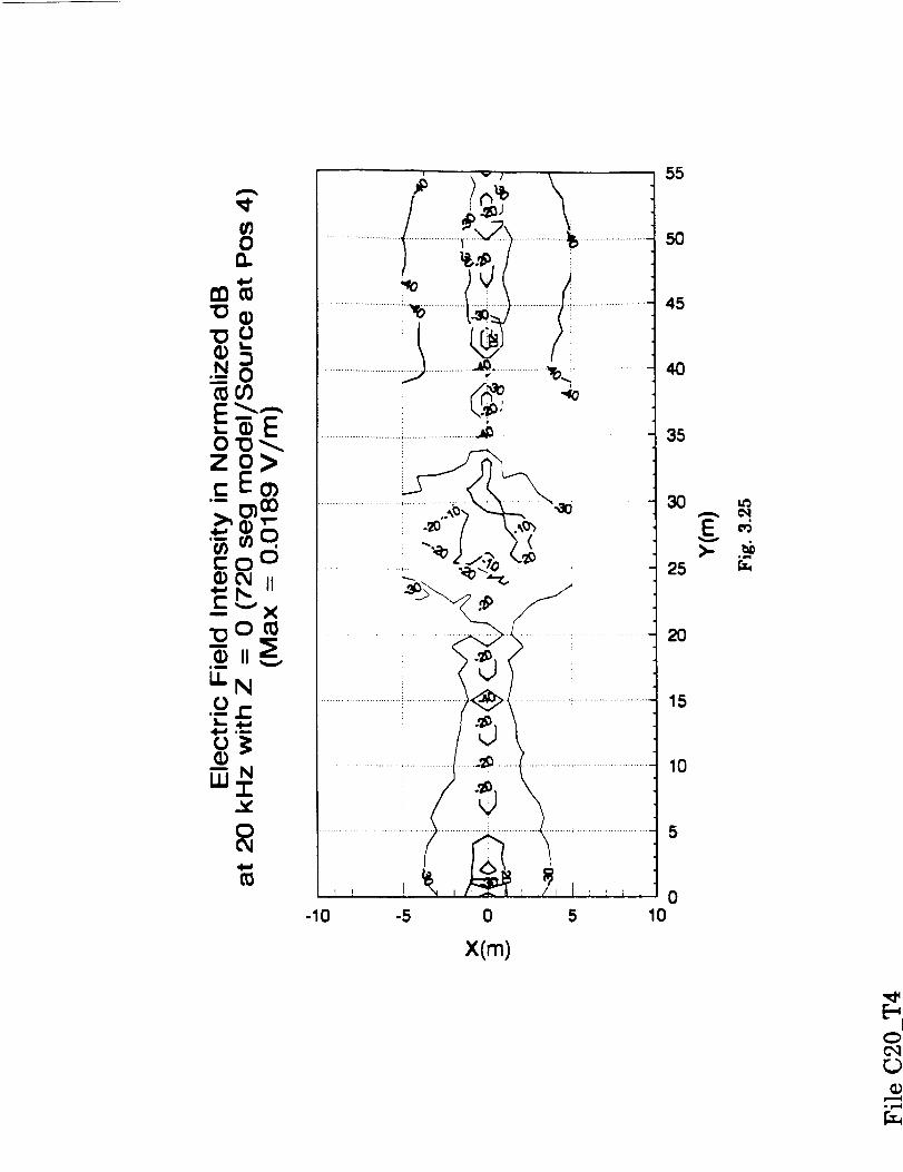
3.2 Method-of-Moments Wire-Grid Model of Space Station Freedom

The method-of-moments may be used to find the conducted currents and fieldsradiated from sources on the space station. Early work used a simple wire model

embedded in a zero-order plasma to determine the near-field electric fields. The

model was then improved by more accurate modelling of the habitation/laboratorymodule and the addition of solar panels. The latest model is shown in Fig. 3.10. This

model is constructed using a wire mesh with 720 wire segments.It is interesting to note that the European Space Agency is using the same

electromagnetic analysis technique to develop EMC models of spacecraft (ESA report

dated 8-28-91). Specifically, the method of moments is used to calculate the currents

and the near electric field for a spacecraft excited by a voltage source. The method

uses triangular surface patches rather than a wire grid to model the structure. The

referenced report indicates that future work will include time-domain solutions,

excitationby current sources as well as voltagesources,and the capabilityto include

35

dielectric materials as well as conducting surfaces. This work has apparently not

included the effects of a surrounding plasma, probably because the applications

currently being considered involve satellites in orbit above the ionosphere, in which

case free space is a reasonable assumption.

The wire-grid model of the space station has been analyzed by the

Electromagnetic Environmental Effects Laboratory at the Georgia Institute Research

Institute using the General Electromagnetic Model for the Analysis of Complex

Systems (GEMACS) computer program, which is a commercial method-of-moments

electromagnetic analysis program. The program assumes free-space conditions, so

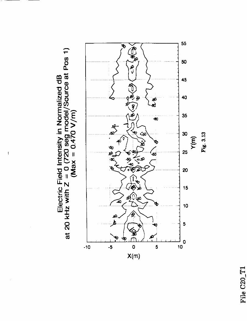
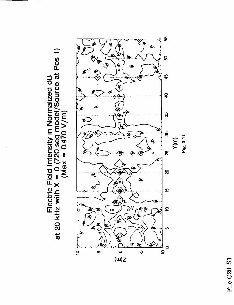
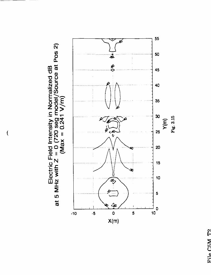
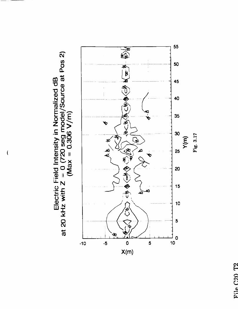
the presence of the ionospheric plasma is not accounted for.Four sets of calculations have been made, one for each of four different source

configurations, two locations and two polarizations, as shown in Fig. 3.10 that are

labelled #1, #2, #3, and #4. Two source frequencies, 20 KI-Iz and 5 MHz, are

considered for each source location and the distribution of the electric field is

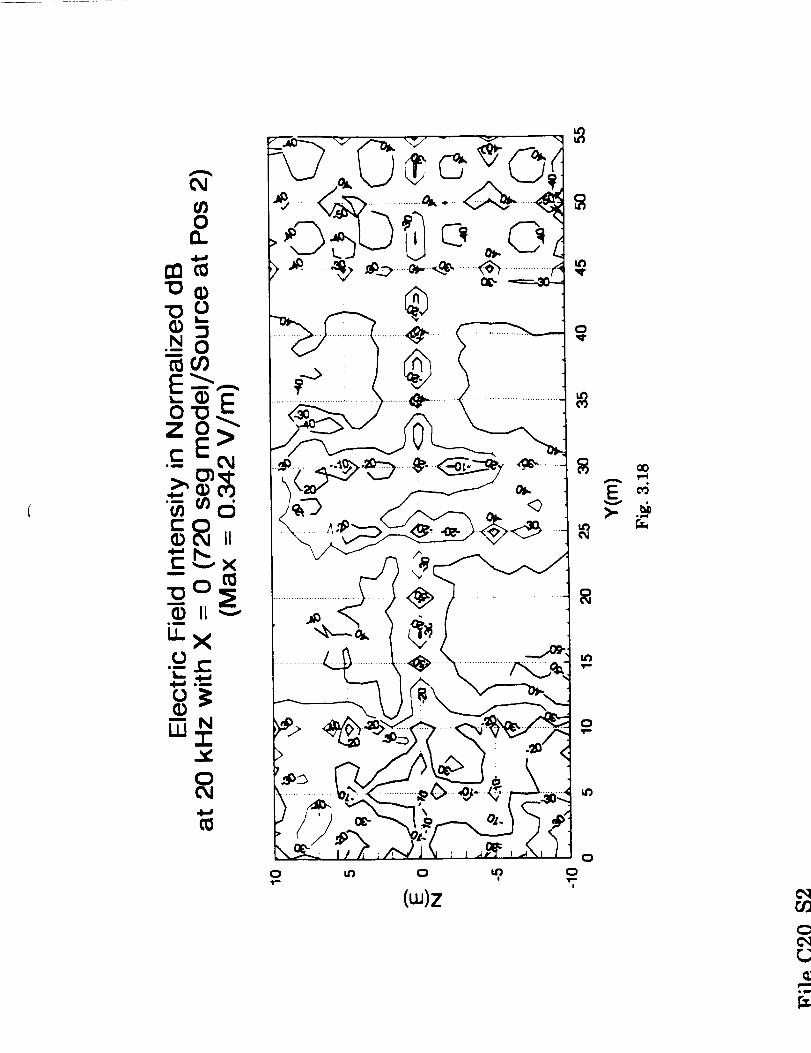
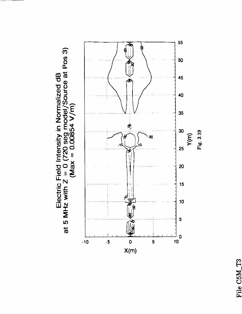
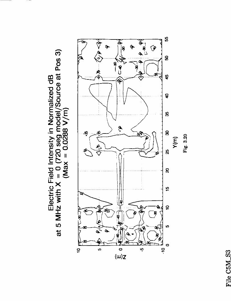
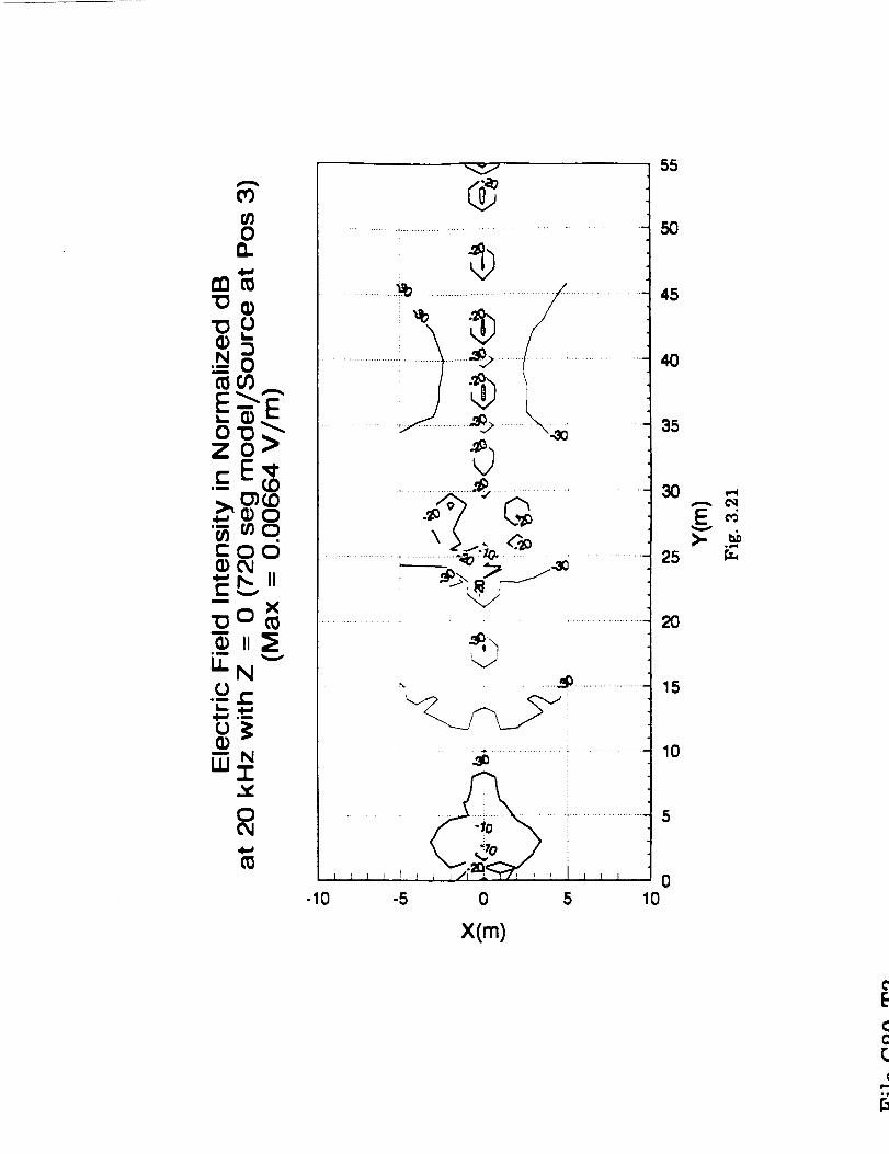
displayed in two planes, the x = 0 plane (Side view) and the z = 0 plane (Top view),

as defined in Fig. 3.10. A total of 16 calculations have been made and graphs of the

results are enclosed in this report as Figs. 3.11 - 3.26. The key to the graphs is

shown in Table I.

Each of the graphs shows contours of electric field strength in dB llV/m for a

one Volt source at the locations shown in Fig. 3.10. The reference for the dB scale

differs from that used in Figs. 3.8 and 3.9 in that the reference level (0 dB) is set at

the source resulting in a relative dB scale, whereas the simple wire model results

displayed in Figs. 3.8 and 3.9 were on an absolute basis. The only practical difference

is that the contours displayed here show negative dB values.

While calculations have been made for 20 KHz and 5 MHz (the 250th harmonic

of 20 KHz), the 20 KHz results are of the most interest. The 20 KHz results for the

source at location 1, top (file C20_T1) and side (file C20_$1) views, show the locations

of high and low field strength. In particular, they show, as in the previous results

for a simple wire model, that the presence of the conducting structure results in

higher electric fields away from the source than would exist if the structure were not

present. As previously explained, electric currents in the structure serve as atransfer mechanism for the electric fields.

Computer Visualization

The model shown in Fig. 3.10 may be viewed and rotated on a color monitor.

An IBM-compatible PC with 512 Kb memory, (preferably) a hard disk, and a mouse

is required. A freeware program called 3dv may be used.

First create a directory on the hard disk called 3D and switch to this directory.

Then insert Disk #1 into the 3.5" floppy disk drive, switch to directory 3D, and copy

all filesto the hard disk (usually drive C:). The model may be viewed as follows:

type 3dv (upper or lower case)

36

use the mouse to clickon the correctgraphics mode (ifnecessary)

use the mouse to clickon the o bulletto the leftof FILE

use the mouse to clickon SSF.3DV

use the mouse to clickon the o bulletto the leftof SHOW

rotate the model by moving the mouse

when through viewing, clickeithermouse button

use the mouse to clickon the o bulletto the leftof EXIT

The 16 calculated method-of-moments results for the wire-grid model may be

viewed on a color monitor. An IBM-compatible PC with 512 Kb memory, (preferably)

a hard disk, and a mouse is required. A graphics program called GraphTools,

licensed from 3-D Visions Corporation, may be used.

First create a directory on the hard disk called GT and switch to this directory.

Then create a subdirectory on the hard disk called TMP. Then insert disk #2 into the

3.5" floppy disk drive, switch to the floppy disk drive, change to directory GT, and

copy file GTOOL.EXE to the hard disk (usually drive C:). Then switch back to the

hard disk and change to subdirectory TMP. Then switch back to the floppy disk drive

and change to subdirectory TMP. Copy all 33 files in TMP to the hard disk (usuallydrive C:). Then switch back to the hard disk and change to directory GT. Run

program GTOOL to create the GraphTools graphics package. When the program hasfinished running, delete GTOOL.EXE. The contour graphs may be viewed as follows:

type gt (upper or lower case)

from the menu, use the mouse to click on File

use the mouse to clickon Directory

use the mouse to clickon OK

use the mouse to click on File

use the mouse to clickon Load

press F3 to view the available files

use the mouse to clickon the filethat isto be plotted(seeTable I)

37

use the mouse to click on OK

use the mouse to click on Redraw

to view another file,click on File, Load, and press F3 as before

use the mouse to click on Quit when finished

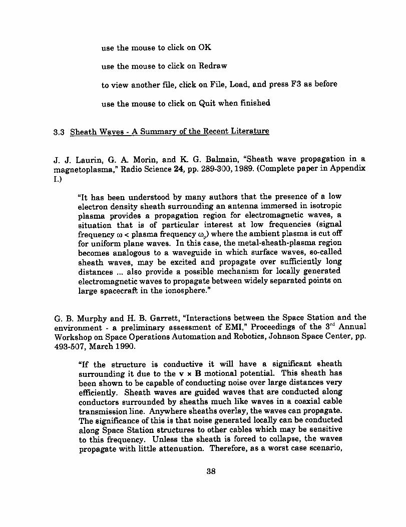
3.3 Sheath Waves - A Summary. of the Recent Literature

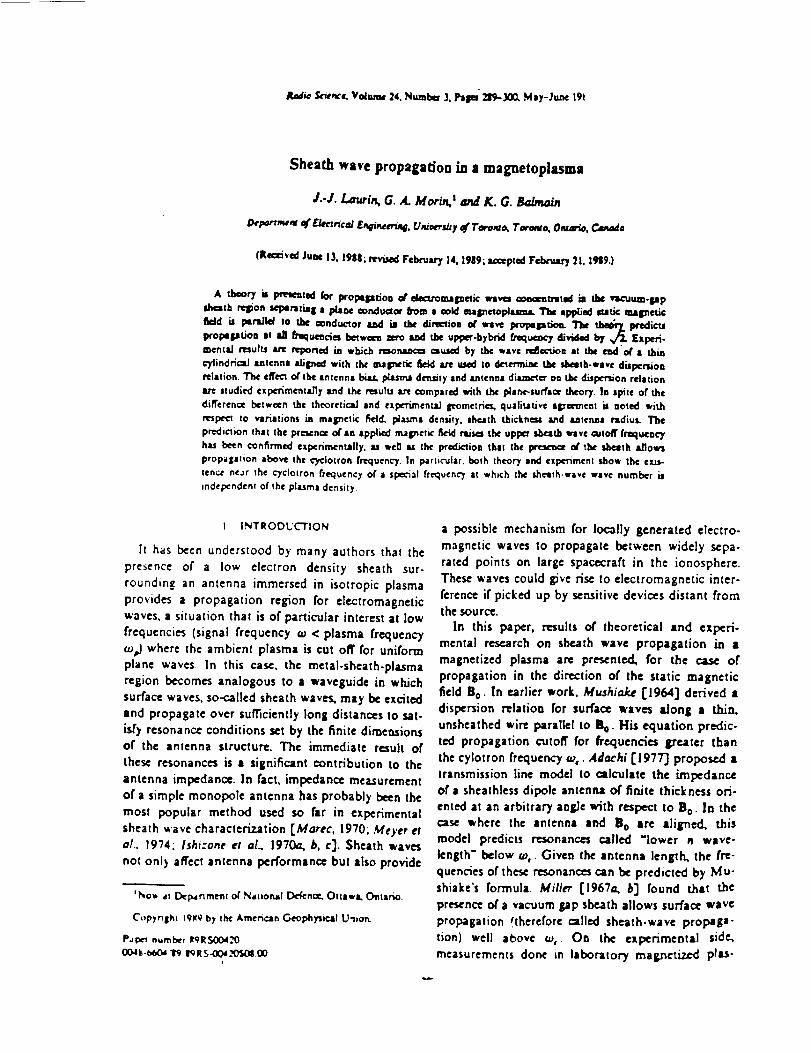
J. J. Laurin, G. A. Morin, and K. G. Bahnain, "Sheath wave propagation in a

magnetoplasma," Radio Science 24, pp. 289-300, 1989. (Complete paper in Appendix

I.)

"It has been understood by many authors that the presence of a low

electron density sheath surrounding an antenna immersed in isotropic

plasma provides a propagation region for electromagnetic waves, a

situation that is of particular interest at low frequencies (signal

frequency co< plasma frequency COp)where the ambient plasma is cut off

for uniform plane waves. In this case, the metal-sheath-plasma region

becomes analogous to a waveguide in which surface waves, so-called

sheath waves, may be excited and propagate over sufficiently long

distances ...also provide a possible mechanism for locally generated

electromagnetic waves to propagate between widely separated points on

large spacecraft in the ionosphere."

G. B. Murphy and H. B. Garrett, "Interactions between the Space Station and the

environment - a preliminary assessment of EMI," Proceedings of the 3 rd Annual

Workshop on Space Operations Automation and Robotics, Johnson Space Center, pp.

493-507, March 1990.

"If the structure is conductive it will have a significant sheath

surrounding it due to the v x B motional potential. This sheath has

been shown to be capable of conducting noise over large distances very

efficiently. Sheath waves are guided waves that axe conducted along

conductors surrounded by sheaths much like waves in a coaxial cable

transmission line. Anywhere sheaths overlay, the waves can propagate.

The significance of this is that noise generated locally can be conducted

along Space Station structures to other cables which may be sensitive

to this frequency. Unless the sheath is forced to collapse, the waves

propagate with little attenuation. Therefore, as a worst case scenario,

38

we assume that cables placed anywhere externally on the Space Station

may be within a sheath which is connected to a source of noise via the

structure-sheath coax transmission line."

K. G. Bahnain, H. G. James, and C. C. Bantin, "Magnetoplasma sheath waves on a

conducting tether in the ionosphere, with applications to EMI propagation on large

space structures," Proceedings of the 4th Annual Workshop on Space Operations

Automation and Robotics, Johnson Space Center, pp. 646-654, January 1991.

(Complete paper in Appendix II.)

"The evidence suggests that, on any large structure in low earth orbit,

transient or continuous-wave electromagnetic interference, once

generated, could propagate over the structure via sheath waves,

producing unwanted signal levels much higher than in the absence of

the ambient plasma medium."

3.4 Finite-Difference Time-Domain Modeling of the Ionosphere

T. Kashiwa, N. Yoshida, and I. Fukai, "Transient analysis of a magnetized plasma

in three-dimensional space," IEEE Trans. Antennas Propag. 36, pp. 1096-1105, 1988.

Abstract

In recent years electromagnetic analyses of magnetized plasma have

become important in various fields. Because of gyroelectric anisotropy

with dispersion characteristics, the analysis is complicated, and three-

dimensional treatment is indispensable. For efficient three-dimensional

analyses in the time domain, the finite-difference time-domain method

and the transmission-line-matrix method are generally used. However,

until now these methods do not seem to have been applied to gyrotropic

anisotropy with dispersion in the time domain. A new method was

recently proposed for transient analysis in three-dimensional space

based on the equivaleknt circuit of Maxwell's equations and formulation

by the Bergeron method. In this method, magnetized cold plasma, that

is,gyroelectric anisotropy with dispersion, isformulated by adapting the

trapezoidal rule to the characteristic equation of motion of the plasma

in the time domain. The formulation of the magnetized cold plasma in

three-dimensional space and in the time domain by the present method

is described. The two principal problems, transverse and longitudinal

propagation, are studied. By examining these results, the validity of

this formulation is demonstrated.

39

R. J. Luebbers, F. Hunsberger, and K. S. Kunz, "A frequency-dependent finite-

difference time-domain formulation for transient propagation in plasma," IEEE

Trans. Antennas Propag. 39, pp. 29-34, 1991.

Abstract

Computation of transient electromagnetic propagation through plasma

has been a difficultproblem. Frequency domain solutions are available

for one or two dimensions and stratifiedplasma geometries. Transient

solutions have been obtained via transformations to the time domain, or

by microscopic solution of the equations of motion of the charged

particles. The finite-differencetime-domain (FDTD) method is capable

of explicitly computing macroscopic transient electromagnetic

interactions with general three-dimensional geometries. However,

previous FDTD formulations were not capable of analyzing plasmas for

two reasons. First, FDTD requires that at each time step the

permittivity and conductivity be specified as constants that do not

depend on frequency, while even for the simplest plasmas these

parameters vary with frequency. Second, the permittivity of a plasma

can be negative, which can cause terms in FDTD expressions to become

singular. A new FDTD formulation for frequency dependent materials

(FD)2TD has been developed, which removes the above limitations. In

a previous paper (FDfTD was applied to computation of transient

propagation through a polar dielectric. In this paper, we show that

(FD)2TD may also be applied to compute transient propagation in

plasma when the plasma can be characterized by a complex frequency-

dependent permittivity. While the computational example presented in

this paper is for a pulse normally incident on an isotropic plasma slab,

the (FD)_TD formulation is fully three-dimensional. It can accomodate

arbitrary transient excitation,with the one limitation that the excitation

pulse must have no zero frequency energy component. Time-varying

electron densities and/or collision frequencies could also be included.

The formulation presented here isfor an isotropicplasma, but extension

to anistropic plasma should be fairlystraightforward.

P. M. Franke and L. J. Nickisch, "Finite Difference - Time Domain solution of the

Maxwell equations for the dispersive ionosphere," Proceedings of the 1991 APS/URSI

International Symposium, London, Ontario, p. 85, June 1991.

Abstract

The Finite Difference -Time Domain (FDTD) technique isa conceptually

simple, yet powerful method for obtaining numerical solutions to

4O

electromagnetic propagation problems. The application of FDTD

methods to problems in ionospheric radiowave propagation is,however,

complicated by the dispersive nature of the ionospheric plasma. In the

time domain, the electric displacement is the convolution of the

dielectric tensor with the electric field, and this convolution is

untractable in the nearest neighbor FDTD approach.

This difficultycan be avoided by returning to the constitutive relations

from which the dielectric tensor is derived. By integrating these

differential equations simultaneously with the Maxwell equations,

dispersion (and absorption) is fully incorporated. The method is shown

to be accurate by comparing to a known analytic solution for a special

case.

41

7

IONOSPHERE CHARGE DENSITY1986 International Reference Ionosphere

">,,4

°--

bqC(1)

"U

q_U_

U_t-C)

A

ro

EO

Cno

_J

6

I

3

2

0

mostly t' 4'

t,'

NO+,02 +,..": ,'I

/

• I

I

I

I

I

I

I

I

I

r "I

,,f..". ....... I I ...................... -'--'t--._. I .......................

"'""- 1. "_1- ......

'""'-.,,, mostly

"-. H+,He+"°,o°.

-..

_°-.,.,"-._.

For Equatorial Orbits,

:: Sunspot number: 75,

_1- J _ T -r

200 400 600

e- max...............O+ me x

e- min

........ O+ min

T 1

8O0

Altitude (km)

Fig. 3.1 Ionospheric charge density as a function of altitude.

_,. J

Fig. 3.2 Plasma frequency fp versus electron density N.

|.l

_LO

G0 I..ll

m

e_

._ 1.0

O.ll

O.¢P

0.1

N - Zx_O _" #/m °

_; - O.SzIO _" #/m"

N - O.OSxIO ss #

| i • _ • ! i T | • i i |

| tO

Frequez_cy (t/Hz)

Fig. 3.3 Attenuation vs frequency for speci_ed electron densities.

I00

150

100

_ so

0I

u

-SO--

-100

it Free Sp_ce........ N = 16' _l/m=......N -- I0 I/m =

..... N = I0 Is _/m=

-_ ,_.-,._,_,, -,.-...-,::.__,,

%%%

- f - 20 kHz

-- 111i1-111[11111111111111111111 iil111iiii111111 iiii

o zo 4o ,o eo 1ooRadius (m)

%%%%%%%%%%%%%%%%% %_

%%%%%%%%%%%%%%%%%

Fig. 3.4 Effect of varying the electron density on the electric field.

Z Seg_t_MO_ODOIt

$o,._-ce

I

l

Fig. 3.5 Wire model with a short monopole antenna excited at one end.

MonopoLe Source on End of 100 m Structure

U

O II LO tl N I N

Pulse Number

N

Fig. 3.6 Current along a 100 m wire with a monopole source at one end.

lOOm

T25tn

]T

_m

1..J

Fig. 3.7 Simple wire model of Space Station Freedom.

\

6O

mo Cl

o N

0

I I I

0

I

I I

LD

(cu) .t

I

\

i.--i

O

I

I

I

,/I

I/

1

I/

I/

I/

I/

II

I/

LZZ

x_

t_

(a)

(b)mm

ml

#i:_ ,2

Fig. 3.10 (a) Wire-grid model of the space station. (b) Section of solar panelshowing the location of the two sources and the two polarizations.

C

8B.

_n_

"00

:_-r.3moo

B_E

E x

_'NO

'r- e-

--Nw n-

20

15

10

5

0-10 -5 0 5 10

X(m)

0

,iii,im

"IC}_"00QL

.N 0m

z o>.C

Qm •

_ II

E_x

X0

mmLe"

0

(w)z

8

v-iA

E _>- ._

A

_Im

0Q..iwa

_m"o_..oo

.N0c0_E_L_po_Ezo_

'g mo

m

.O oo__ _

U- N

0 e.|m

--NU.I-r

0

-10 -5 0 5

x(m)

55

5O

45

40

35

3O

25

2O

15

I0

5

010

)- ._

,T=.

013.

"00l_

•_ 0m

E__.A

.c_E o

_¢_."_ mO

_ x-oo_(P II_

u..xO..Clu

L._

CD"-- N1117-

.=_

C}04

(w)z!

EV

>" ._

f/10n

rnc_

L

imm

E_A

ZO>

E_x

u-N(J._- c-

m NLUn-

143

v___, 55

..................................................._ ........................._..........................45

.............................!..........................................! .................

-10 -5 0 5

4O

35

3O

25

2O

15

10

0I0

x(m)

.m=l

(w)z

A

EV

ommmm

r_

Cq

8n

.N _O

_Ec"

_x

._ IIU-N0

tn

m NLU-r

0t_

_-so 55

.......................

, ; ' I I 1 l 1 I !

-10 -5 0 5

4O

35

3O

25

010

x(m)

10

15

2O

A

0B.

tO

0B.

m_"0

z_>._E_

_ X

O•_ r"+.,.__

m Nm I

It)

55

NI

45

4O

35

................................................."'................_s

......................... 20

1

............................:..............._ " 15

i

........................................_ ............................10

-i............................................)"_........................7...........................s

' ' I I I J z_-' ' J ' 11 I I L 0-10 -S 0 5 10

X(m)

tO

0

"00L

'.._--0

_°o>E_

fflOcod

.__ e-_ °_

D Nm I

O

55

.........................:......................._.,>............:..............40

............_ ............*"_'>......."_".30...... 35

.............................___.._c,o............

V

_" ......... _ .........................15

................................................... 10

...... _ .............................. 1 5

I 1 1 I ! 1 0

-10 -5 0 5 10

3O

25

X(m)

.N 0i

_CO

It}

0_r

ZO>.c:E,--

O.)CO

_oc_(P_ II*" l",-t'v xm

.__ II_

u-xU t-Dm

-- NLU.I-

E]

Ev

>" ._

13.

"00L_

=0

u__0_

__E_

_0

_x"_0_

_ ii _

N0"F- _-_,.__

4.a

-10 -5 0 5

2O

15

10

5

' 010

X(m)

,¢

.c_E_o _ _ ...

" N

z o>r- O_

0

5

X(m)

35

15

I0

010

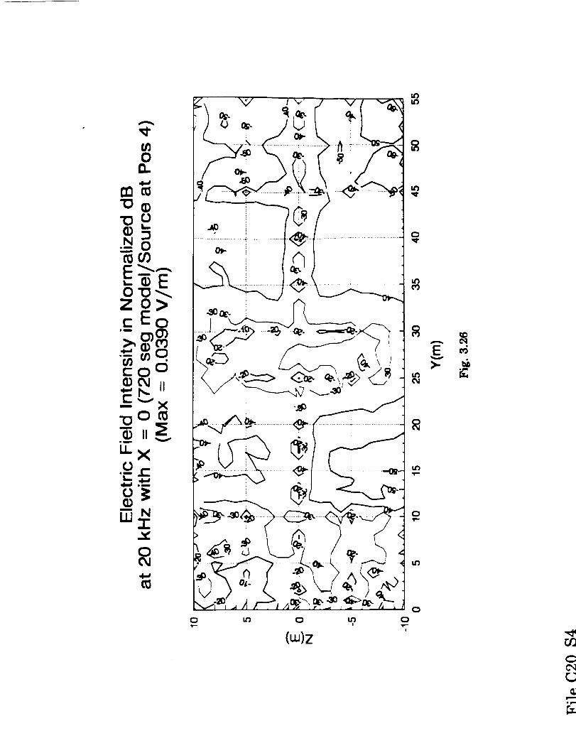
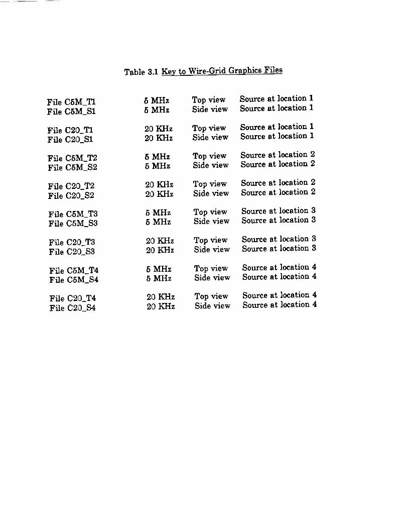
Table 3.1 Key to Wire-Grid Graphics Files

File C5M_TI

File C5M_S15 MHz Top view Source at location15 MHz Side view Source at locationI

File C20_TI

File C20S120 KHz Top view Source at location120 KHz Side view Source at locationI

File CSM_T2

File C5M_$25 MHz Top view Source at location25 MHz Side view Source at location2

File C20T2File C20_$2

20 KHz Top view Source at location220 KHz Side view Source at location2

File CSM_T3

File C5M_$3

5 MHz Top view Source at location35 MHz Side view Source at location3

File C20T3

File C20_$320 KHz Top view Source at location320 KHz Side view Source at location3

File CSM_T4File C5M_$4

5 MHz Top view Source at location45 MHz Side view Source at location4

File C20_T4

File C20_$420 KHz Top view Source at location 420 KHz Side view Source at location 4

Appendix I

J. J. Laurin, G. A. Morin, and IL G. Balmain, _Sheath wave propagation

in a magnetoplasma," Radio Science 24, pp. 289-300, 1989.

/b:dio .r_-_ncc,V_ume 24. Numb_ 3./:alP::"219-300, May-June t9t

Sheath wave propagation in a magnetoplasma

J.-J. LawM, G. ,4. Morin, I and K. G. Balnufin

oepeer_nr qf'K_'trical £nCintermll, Unieositt qf Toremo, Toronto, Onurio, _mada

(Rec=ived Juan 13, 1988; revised February 14, 1989; accepled February 21, t919.)

A thaory is pr_'nmd k)r propapr;o= d decuonup¢6c wav_ coocrnmlted ia tlx v'_uum.ppsh,,--tb re2pon =elXtratia| a pla_¢ cond_ _ a =old mal_etoplasmL The aPl_ed static ',,-I_¢dc

f_ld is F_'ldlel to tJbcconductor tad i= the &rl_ion of wuve pml_p_a. _ _ pcedictsproi_pdoe at _n I'mclu_,,aciahe,wee= ze'e and _ upger-bybrkl fmqu_'7 divided b7 _ Experi-memaJ results mat nq_ned us which reso_ =tu.ted by the wave re_ec-,/oeat thee_lof • thin

cylindrical tmenna atilp,Ved with the malp'_ric fudd are uted to determLn¢ the sheath-u, av¢ dispertionrelation. TIw effet't of the antenna _ plasm= den.airyand tmenna ditmeter on [hc d_ix-'_on relation

are studied exp_mema]ly and the r_utu itre compared with the Idane-$urfsce theory, la spite of thedifferenoe betwe=n abe IheoreticaJ and ¢xfx'rtmentitl i_-ometr_es,qualitative algre¢.ment is noted withmspec_ to variations in malpnedc field, idzsma density, sheath thickness _d _ten.na rldius. "rb¢

pmdi_ion that the preseno¢of'an tppGed malp_¢6¢ _ rt/_ the upp= _th wave ,'utoff (requenc7has been confirmed ezperiment=lly, as _,ell as th_ predk'tion that the _ of tl_ d_u=th _1o_propagation above the cyclotron frequency. In particular, both theory and experiment thow the exit-

I¢nc..enear the cyclotron frequency of a spe_al frequency at _hJch the the-ath-wav¢ wave number isindependent of the plasma density.

I INTRODL'CTtON

It has been understood by many authors that the

presence of a low electron density sheath sur-

rounding an antenna immersed in isotropic plasma

provides a propagation region for electromagnetic

waves, a situation that is of particular interest at low

frequencies (signal frequency _ < plasma frequency

cop) where the ambient plasma is cut off for uniform

plane waves. In this case, the metal-sheath.plasma

region becomes analogous to a waveguide in which

surface waves, so-called sheath waves, may Ix excited

and propagate over sufl3ciently long distances to sat-

i_y resonance conditions set by the finite dimensions

of the antenna structure. The immediate result of

these resonances is • significant contribution to the

antenna impedance. In fact, impedance measurement

of a simple monopol¢ antenna has probably been the

most popular method used so far in experimental

sheath wave characterization [Marec, 1970; Meyer et

al.. 1974; Ishi:one e_ al, 1970=, b, c]. Sheath waves

not onl) affect antenna performance but also provide

'No_ _ Ekl_nm.t of Nalioul Dd'en_., Ottt_,t. Ore,rio.

CopYnlht 191(9by taw American G¢oph_i,"=l U'_Jo_-

P._pt"_numb¢_ ItgR_O0_."OOOal_.be_ 1"9I_RS-O0_."OSO_O0

a possible mechanism for locally generated electro-

magnetic waves to propagate between widely sepa-

rated points on large spacecraft in the ionosphere.

These waves could g_ve rise to electromagnetic inter-

ference if picked up by se_itive devices distant from

the source.

In this paper, results of theoretical and experi-

mental research on sheath wave propagation in a

magnetized plasma are presented, for the case of

propagation in the direction of the static magnetic

field Bo. In earlier work, Mv_hi_.e [1964] derived •

dispersion relation for surface waves =long • thin,

unsheathed win= parallel to Bo. His equation predic-

ted propagation cutoff for frequencies greater than

the cylotron frequency w,. Adachi [1977] proposed •

transmission line model to calculate the impedance

of a sheathless dipole antenna of finite thickness ori-

ented at an arbitrary angle with respect to B o. In the

case where the antenna and B e are aligned., this

model predicts resonances called "lower n wave-

length" below w,. Given the antenna length, the fre-

quencies of these resonances can be predicted by Mu-

shiake's formula. Miller [1967=, b] found that the

presence of a vacuum Sap sheath allows surface wave

propagation (therefore called sheath-wave propaga-

tion) well above ¢o,. On the experimental side,

measurements done in laboratory magnetized ply-

't-90 LAURIN ET AL.: SHEATH WAVES IN MAGNETOPLASMA

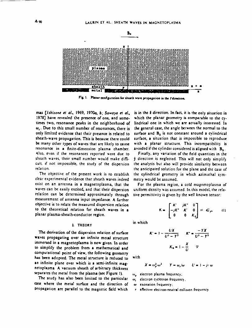
L thFiB i. PLIaIr mnfigursdon for she.ath _1_ prol_|ation Ja tk ldirlaion.

rnas [lshizone et al., 1969, 1970a, b; $awaya et al.,

197g] have reve_Jed the presence of one, and some.

times two, resonance peaks in the neighborhood of

w,. Due to this small number of resonances, there is

only limited evidence that their presence is related to

sheath-wave propagation. This is because there could

b¢ many other types of waves that are likely to cause

resonance in a finite-dimension plasma chamber.

.Also, even if the resonances reported were due tosheath waves, their small number would make diffi-

cult, if not impossible, the study of the dispersionrelation.

The objective of the present work is to establishclear experimental evidence that sheath waves indeed

exist on an antenna in a magnetoplasma, that the

waves can be easily excited, and that their dispersion

relation can be determined approximately through

measurement of antenna input impedanoe. A furtherobjective is to relate the measured dispersion relation

to the theoretical relation for sheath waves in a

planar plasma-sheath-conductor region.

2. THEORY

The derivation of the dispersion relation of surface

waves propagating over sn infinite metal structure

immersed in a magnetoplasma is now Ipven. In order

to simplify the problem from a mathematical and

computational point of view, the following geometryhas been adopted. The metal structure is re.duced to

an infinite plane over which is = semi-infinite mag-netoplasma A vacuum sheath of arbitrary thickness

separates the metal from the plasma (see Figure !).

The study has also bccn limited to the particular

case where the metal surface and the direction of

propagation arc parallel to the magnetic field which

is in the t direction. In fact, it is the only situation in

which the planar geometry is comparable to the cy-lindrical one in which we are actually interested. In

the general case, the angle between the normal to the

surface and B0 is not constant around | cylindrical

surface, a situation that is impossible to reproduce

with a planar structure. This incompatibility is

avoided if the cylinder considered is aligned with Bo.

Finally, any variation of the field quantities in the

_'directionisneglected.This willnot only simplify

the analysis but aim will provide similarity between

the anticipated solution for the plane and the case of

the cylindricalgeometry in which azimuthal sym-

metry would be assumed.

For the plasma region, a cold magnetoplasma of

uniform density was assumed. In this model, the rela-

tive pcrmittivity is given by the well known tensor:

in which

_KoK j K " _1K= " K' -- E: r, (I)

0 K

UX - YXK'=I K'=_

U _ - y_ Us_ y2

with

XKo" I---

Ud,

X - ,o=,,=o' Y = cv,/c_ U = I -/_'=J

au, electron pl=cma frequency;

oJ, electron cyclotron frequent);

w e,,catstion frequency;

r effective electron-neutral colhsnon frequency.

PRECEDING P/31GE BLANK P_O-i FILI_ED

LAURIN ET AL.: SHEATH WAVES I'N MAGNETOPLASMA 291

The SI system of units has been adopted in this

paper. Also, all the field quantities, except Bo, will be

manipulated as phasors.In the case of harmonic time dependence of the

type es-, Maxwell's equations are written

P x H -_¢0 g- £ (2o}

V x E:- -/o,,_ o H (2b)

V.K-E=0 (2c)

V .H - 0 (20

for the plasma region, and

V x H -,kor_ £ (_=)

V x £ - -jW_o H (3/,)

V. E = 0 (3c)

V.H=0 (_r)

in the vacuum-gap sheath re,on. Assuming a z vari-

ation of the type e -'_, where k is the complex propa-

gation constant, one can write the V operator as

,.0+,_,.)2.1. Solution in the sheath

Using this definitionof V. the components of E

and H can be convenientlyseparatedinto two inde-

pendent setsand the generalso[utiontoequations(3)

is writtenas a superposition of a TM and a TE

mode :

TM mode

TE mode

where

H, - C cosh(hx}+ F..sinh (kx)

k£, - -- h',

oJ(o

hB, - ---- (C sinb (k=) + E cosh (hx))

/o._ o(4c)

H I

£, - D sinh(kx)+ F cosh (k=)

-kH, - -- £,

_14o

-k- ----- (D cosh (/ur) + F sinb (kx))

]W#o

k - (*_ - #_j,a

in which. ,8o= - oa=_/J0 . C, D, E and F are arbitraryconstants. The boundary conditions at the metal sur-

face (x = 0) require that E, = 0 and E, = 0 This sets

£ = ¥ = 0 in (4) and (5).

7.2. Solution in the piog_

Unlike the sheath r_g_on,the snisotropic nature of

the plasma makes impom'bk the scpara6on of the

field components into two independent sets. There-

fore it is only necessary to solve for one field compo-nent from which =11 the =hers can be derived. The

choice of this field component may seem purely arbi-

trary • priori. The choio¢ of a component belongingto the TM mode _ lead to a more genera] solution

because, as it w_] be seen later, the components of

the TE wave va.t_h if m, is reduced to O. Also, in

order to ensure con/'or_(7 with the existing litera-

ture, the solution for E, is found.

After a few a]gebraJc manipuladons [Laur/n,

1986],equations (2)can bc combined intothefollow-

ing:

(v+: - =_Xv: - =])£, - 0 (6)

where Vt is the component of V perpendicularto the

i direction.The quantities=I and =_ are solutionsof

the biquadraticequation,

with

£, = Ae"" + Be""

(5=) However, in the particular case where

bz -4=c =0(sb)

the general solution for E:Js

(_) £: - lax + BW"with

o:" +_+ c = 0 (_a)

(St)

a = K' (Tb)

b ==_2o(K'_- K "=+ K'K o) - k=iKo + K3 (7c)

c = ,8_oKo(K'= - K"=) - 2/3_k=KoK'+ k'K o (7_

With Vt = (8/¢?.xhLthe general solution to (6) is

E: - A_" + Be"" + Ge'"" + it "',=

A, B, G and i are constants, ff we choose =_ and =z

such that their real parts are negative, the solution

for E= remains physically possibly only if G = I ,- O.

Thus,

($)

(9)

(I0)

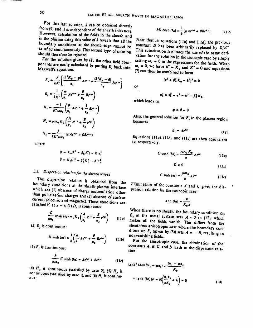
292 LAURIN ET AL.: SHEATH WAVES IN MAGNETOPLASMA

For this last solution, k can be obtained directly

from (9) and it is independent of the sheath thickness.However, calculation of the fields in the sheath and

in the plasma using this value of t reveals that aU the

boundary conditions at the sheath edge cannot besatisfied simultaneously. This second type of solution

should therefore be rejected.

For the solution given by (g), the other field corn.

ponents are easily calculated by putting E, back intoMaxwell's equations.

<_= Ko(P-p._ K')- K'=_

o = Ko(P - Po_K'J- K'=I

i

kO cosh(ks) = _ (+tAd" + OBd") (! t=3

Note that in equations (lib) and Old), the previous

constant O has been arbitrarily replaced by D/K"This substitution facilitates the use of the same deri-

vation for the solution in the isotropic case by simply

_tting w, - 0 in the expressions for the fields. When

w, = 0, we have K' = K o and K" - 0 and equations

(7) can then be combined to form

(=2 + I_ g. - t') 2 - 0

or

=,_" =I " ==" t _ -/q x.

which leads to

e=#-0

Also, the general solution for E, in the plasma regionbecomes

£, - At" (12)

Equations (I la), (I lb), and (I It) are then equivalent

to, respectively,

C cash(hs)= J_c°g.-----_°A#" (t3a)a[

D ,= 0 (13b)

2.3. Dispersion relation for t_ sheath waves

The dtsl:_rsion relation is obtained from the

boundary conditions at the sheath-plasma interface

which are (l) absence of charge accumulation other

than polarization charges and (2) absence of surface

current (electric and magnetic). Those conditions are

_tisfied if, at x = s, (1) D, is continuous:

, )cash (ks) - jK o _" + -- f'" (lla)c0¢, \=a %

(2) Et is continuous:

, )D sinh (ks) = _ At,'" + -- B_" (l lb)=3

13) E, is continuous:

kC sinb (Es)- At"" + J_' (]1c)

j(o£ o

(4) H, is continuous (satisfi_ by case 2), (5) H t is

continuous (satisfied by case Ik and (6) H, is continu-ous:

C sinh (ks)= /if-? At ,_ (I3c)h

Elimination of the constants A and C gives the dis-

persion relation for the isotropic case:

¢1lane (_) -

Kok

When thereisno sheath,the boundary condition on

E, at the metal surface sets A = 0 in (12k whichmakes all the fields varush. This differs from the

sheath)ess anJsotropic case where the boundary con-

dition on E, (given by (8)) sets A = -B, resulting in

nonva.rfish.ing fields.

For the anisotropic case, the elimination of the

constants .4, B, C, and D leads to the dispersion rela-tion

t,mnh"(hz)(0== - e=_} + --_)=l -- (Pelf,1

K o

/=.=. \+ tmnb t/u)(¢ -ItX '--"+ hi ,,0

\hK o /(14)

ioi - nasa

Documents