Investigations on driving flow expansion characteristics inside ejectors

Zuozhou CHEN, Chaobin DANG*, Eiji HIHARA

Institute of Environmental Studies, Graduate School of Frontier Sciences, The University of Tokyo, 5-1-5 Kashiwanoha, Kashiwa-shi, Chiba 277-8563, Japan

Email: dangcb@k.u-tokyo.ac.jp

Abstract: This research investigates the Mach wave structure of the driving flow under off-design working

conditions by both numerical and experimental methods. By adopting the method of characteristics as the simulation

model, prediction of the driving flow regime inside an ejector is obtained. The simulation results are further

validated by an experimental visualization method conducted using a Schlieren system. Through this investigation,

the influence of Mach wave on the driving flow boundary development is discussed. The expansion wave from the

nozzle exit increases the driving flow regime in the under-expanded condition, which has a negative impact on

ejector performance. The results show that the Mach wave should be considered when the ejector is operated under

off-design working conditions. The results also demonstrate that an appropriate nozzle structure design was able to

restrain the effect of the expansion wave, which improves ejector performance. The results are significant for

achieving a comprehensive understanding of the mechanism of an ejector, as well as for the applications, such as

ejection refrigeration cycles.

Keywords: ejector, Schlieren photography, method of characteristics, numerical simulation, visualization

Nomenclature

Notations Units subscripts

A Cross-sectional area b Back pressure

A Local sonic velocity d Driving flow

AR Area ratio e Nozzle exit

C Characteristic curve m Mixing section

Cp Specific heat capacity n Surface number inside the ejector

D Diameter max Maximum value

ER Entrainment Ratio s Suction flow

h Specific enthalpy t Nozzle throat

I Information of a grid point (x, y, u, v) x x Direction

Iter Iteration number y y Direction

M Mach number + Left-running Curve

Mass flow rate - Right-running Curve

N Grid number 0 Static condition

P Pressure 1, 2, 3… Numbers of iteration

R Gas constant

T Temperature

U Velocity component in x direction

V Velocity component in y direction

V Velocity

Q Terminologies applied in the finite

differential equations

O

S

Specific heat ratio

Mach angle

Velocity angle

Mach line angle

Flow deflection angle

Δ Constant for axisymmetric flow

1. Introduction Large-scale applications for air conditioning and refrigeration systems consume huge amounts of energy and

cause environmental problems. Efforts to reduce the level of energy consumption in these applications have led to

renewed interest in heat recovery systems. Heat recovery refrigeration systems are an alternative to vapor-

compression refrigeration systems. In these systems, low-grade heat such as solar energy or exhausted heat can be

utilized as the driving energy. The ejection refrigeration cycle is one example of such heat recovery systems, and it

has the following advantages: simple-structure, reliability, and low-cost. In recent years, the number of journal

papers focusing on ejectors or ejection refrigeration cycles has grown rapidly [1]. Ejectors have been investigated

in the field of waste-heat utilization [2] and in ejector–vapor-compression hybrid cycles [3]. In CO2 heat pump

systems, ejectors are employed as expansion devices to reduce throttling losses [4]. In addition, a number of studies

on solar-driven ejection refrigeration cycles [5]-[10] have been conducted.

Fig. 1 Schematic of the ejector and the Mach wave positions

Fig.1 shows the structure of an ejector with the flow regime and Mach wave inside. The ejector comprises of a

motive nozzle and a suction chamber. High pressure refrigerant, known as the driving flow, is accelerated through

the motive nozzle and converted into high velocity flow with low pressure. The suction flow is entrained into the

ejector from the suction flow inlet. The flow from the motive nozzle exit is then divided into two regimes: the

driving flow regime and the suction flow regime. On the shear layer of the driving flow boundary, part of the kinetic

energy from the driving flow is transferred to the suction flow. The two flows will finally mix in the mixing section

and jet outward from the diffuser. The performance of the ejector is described by the parameter ER (the Entrainment

Ratio) and PR (the Pressure Ratio) as shown by Eq. (1), (2).

suctionflow drivingflow/ ER m m (1)

b s ,0/PR P P (2)

In Fig. 1, and , represent the pressure of the driving flow and the suction flow at the nozzle exit,

respectively. There are two locations inside of the ejector where Mach waves may occur. In those locations, the

Mach wave could manifest as an expansion wave or shockwave based on the expansion or compression effect on

the supersonic flow. The driving flow Mach wave may occur at the nozzle exit, and the mixed flow shockwave may

occur in the diffuser, where the mixed flow changes to subsonic from supersonic. There are three conditions for the

driving flow: If is larger than , , the driving flow is in an under-expanded condition and expansion waves will

occur. On the other hand, if is smaller than , , the driving flow is in over-expanded condition, and shockwaves

Driving flow

Input Energy

Suction flow

Throat

Mixing Section Diffuser

Compression shock waves

Suction Chamber

Non-mixing Section

Shear-LayerBoundary

will occur. The ideally-expanded condition is reached if is equal to , . The occurrence of a Mach wave is

usually avoided by optimizing the design of the motive nozzle to reach the ideally-expanded condition. In the one-

dimensional theoretical model, the driving flow condition is usually assumed near the ideally-expanded condition.

The constant-pressure mixing theory proposed by J.H. Keenan et al. [11] and the non-mixing process between the

driving and suction flows proposed by J.T. Munday and D.F. Bugster [12] were adopted to describe the working

process of the ejector. In the models, ER is obtained from the cross-sectional flow areas of the driving and suction

flow in the non-mixing section. Since the ejector structure is fixed, the relationship of the flow areas could be

obtained by Eq. (3), and the calculation process of ER was introduced in the one-dimensional model developed by

Huang et al [13].

s,n d,n m+ =A A A (3)

In applications such as waste heat utilization, a relatively stable heat source temperature could maintain the

optimum-expand condition for the ejector. Yet, in other cases, especially for solar energy utilization, the driving

flow will be in either the over-expanded or under-expanded condition. This is due to the fact that the ideally-

expanded condition cannot be maintained because the solar energy input is fluctuating. Under off-design conditions,

Mach waves may develop and influence the ejector performance. Shockwaves in the over-expanded condition cause

irreversible energy loss in the driving flow. On the other hand, expansion waves in the under-expanded condition

creates radial velocity components in the driving flow, which will reduce the flow area of the suction flow regime.

To employ ejection cycles in solar energy utilization, the influence of Mach wave should be considered. However,

there have not been many studies aimed toward the occurrence of Mach waves and its influence on ejector

performance.

In this research, the Mach wave in the gas-ejector at the off-design working condition is discussed. The influence

of Mach wave on the driving flow expansion, as well as the ejector performance, is investigated numerically and

experimentally. A numerical approach using the method of characteristics model is adopted to predict the driving

flow expansion inside an ejector. The simulation results are further validated by visualization experiments conducted

using the Schlieren photography method. The research reveals the influence of Mach wave on the ejector

performance, which is significant for the application of solar-driven ejection–refrigeration cycles.

2. Prior Work on Model Development of an Ejector Following the models proposed by J.H. Keenan et al. [11], J.T. Munday, and D.F. Bugster [12], Huang et al.

established and validated a one-dimensional model in which an isentropic process was considered for the driving

flow expansion inside of an ejector [13]. Eames also proposed an ejection–refrigeration cycle evaluation method

using the isentropic process, and validated it experimentally with a steam ejection cycle [14]. B.J. Huang et al.

conducted a series of experiments and validated the choking assumption for the one-dimensional model [15]. Fig.

2 (a) shows the working process assumed in the one-dimensional model. Since the driving flow is in the ideally-

expanded condition, the isentropic expansion process described by Eq. (4), (5) is adopted to predict the flow area

for the driving flow regime. As the driving flow expands from the nozzle exit, a hypothetical converging tunnel for

the suction flow is formed by the driving flow boundary and the ejector wall. The suction flow accelerates inside

the tunnel until it reaches sonic velocity.

2 / ( 1)d ,n

2 /( 1)e

(1 ( 1) / 2)

(1 ( 1) / 2)

n

e

MP

P M (4)

( 1)/(2( 1))2d,n d,nd,n

( 1)/(2( 1))2e e e

2 / ( 1)(1 ( 1) / 2)

2 / ( 1)(1 ( 1) / 2)

(1 / M ) MΑ=

A (1 / M ) M (5)

(a) Driving flow boundary by the non-Mach wave

isentropic expansion assumption

(b) Driving flow boundary affected by the Mach

waves in under-expanded condition

Fig. 2 The driving flow expansion inside the ejector

Fig. 2 (b) shows other factors that may occur inside the ejector, such as a Mach wave and a shear layer. Those

factors are discussed in the following studies using both experimental and numerical methods. S.K. Chou et al.

introduced efficiency factors for the nozzle structure and the shear-layer thickness into a one-dimensional model

[16]. K. Mohammed et al. considered the friction loss inside the ejector, and employed polytropic efficiencies to

determine the dimensions of the ejector [17]. Y.H. Zhu et al. presented a two-dimensional model for the suction

flow velocity distribution [18], and further developed the model for both dry and wet vapor ejectors [19]. H. El

Dessouky et al. proposed a model for both choked and un-choked conditions under various backpressures [20]. S.J.

Chen et al. discussed a model for the ejector with a converging mixing cone [21]. J.G. del Valle et al. proposed a

prediction model for driving flow boundary development based on a turbulence model, and built the prediction

model into the one-dimensional model [22]. J.Y. Chen et al. proposed a model that considers the suction flow

velocity at the ejector entrance [23]. K. Matsuo et al. studied nozzle structures and claimed that the nozzle’s exit-

to-throat area ratio was an important factor affecting ejector performance [24]. D.A. Pounds et al. predicted the

ejection refrigeration system performance from the model they proposed with a quasi-1-D assumption for the mixing

section [25]. D. Butrymowicz et al. developed a calculation methodology for an ejection refrigeration system with

an internal heat exchanger [26]. W.N. Fu et al. conducted an investigation on nozzle structures using numerical

simulation, and claimed that nozzle structure design was essential for optimizing an ejector [27]. N.B. Sag and H.K.

Ersoy also conducted experiments on the nozzle structure, and claimed that an optimal nozzle enhanced system

performance by 8 % - 13 % [28].The driving flow Mach wave is considered to be one of the factors that influence

ejector performance. Currently, investigations on driving flow Mach waves are conducted using visualization

experiments and numerical simulations. Y.H. Zhu and P.X. Jiang studied the shockwave characteristics in a Schlieren

system. The driving flow Mach wave from both supersonic and convergent nozzles were observed, and they claimed

that by reducing the first Mach disk length, the ejector performance would be enhanced [29]. The empirical

equations for Mach disk length are further obtained using visualization experiments in the following studies [30]. J.

Gagan et al. combined PIV and numerical simulation methodologies to obtain the appropriate turbulence simulation

model for a gas ejector [31]. A. Bouhanguel et al. conducted visualization experiments using laser tomography

techniques that showed the supersonic flow regime [32]. A.B. Little and S. Garimella adopted the shadow method

and discussed the condensation effect caused by shockwaves inside of the ejector [33].

The under-expanded condition for the driving flow is discussed in this research because in the over-expanded

condition; the driving flow velocity is reduced after passing through the shockwave. At the same time, driving flow

may detach from the nozzle wall and the negative factors make the over-expanded condition inappropriate for the

operation of gas ejector. A.L. Addy proposed the empirical prediction of driving flow boundary from a convergent

nozzle into a free space [34]. A.J. Ruggles and I.W. Ekoto adopted Schlieren photography to investigate the Mach

wave structure of supersonic flow in free space [35]. The method of characteristics (MOC) model is commonly

employed in simulations involving supersonic flow. A.L. Addy and W.L. Chow attempted to employ the MOC

model to predict the driving flow expansion inside of the ejector. They combined the numerical simulation method

Nozzle exit

Hypothetic boundary

Suction flow

Driving flow,

Section n

Expansion Fan Reflected shockwave

Expansion wave

Nozzle exit

Suction flow

Shear layer

with a one-dimensional model, and gave a reasonable prediction of the ejector performance [36]. In this research,

the MOC methodology is also adopted to predict the driving flow expansion inside the ejector. A Schlieren optical

experimental setup is constructed to validate this simulation method. The Mach wave is discussed in terms of the

simulation and experiment results, and the importance of employing an optimized nozzle inside the ejector is also

discussed by simulation.

3. Simulation Methodology (The Method of Characteristics) 3.1 Expansion process of the driving flow

As shown in Fig.3, the driving flow field is divided into three parts, marked as Ⅰ, Ⅱ, and Ⅲ. The three parts

represent the flow field before, inside, and after the expansion fan. In the under-expanded condition, an expansion

fan is formed by a group of expansion waves propagating from the nozzle exit rim. The expansion fan depressurizes

the driving flow pressure to suction flow pressure at the nozzle exit, and gives an out-turning flow angle to the

driving flow. The driving flow pressure will further decrease in flow regime Ⅲ because of this flowing angle. In

regime Ⅲ, when the driving flow pressure is smaller than the environmental pressure, a shockwave will originate

from the boundary to correct the driving flow pressure and flow direction. In summary, the Mach wave is the

propagation of physical disturbances caused by a pressure difference, and the driving flow regime is influenced by

both expansion waves and shockwaves.

The Mach wave could be considered a simple wave if the pressure difference between the driving flow and the

environment on the boundary was infinitesimal. The driving flow undergoes an isentropic process through a simple

wave. In the method of characteristics, because the finite differential method is adopted, the expansion wave and

shockwave are all considered simple waves. The simple wave could be described by the characteristic curve, because

along the characteristic curve direction for each point in the supersonic flow field, the derivatives of the physical

properties of the flow are discontinuous, while the properties are continuous. Therefore, the flow field could be

described by creating a grid of units linked by the characteristics curves as illustrated in Fig. 3. The method

introduced by M.J. Zucrow and J.D. Hoffman is adopted in this study [37] and several assumptions are clarified:

1. The outflow from the nozzle is parallel with unified velocity.

2. The flow field is axisymmetric to the x-axis.

3. The flow is supersonic throughout the driving flow regime.

4. Friction between driving flow and suction flow is neglected. 5. The calculation proceeds under an ideal gas assumption with constant and .

6. The suction flow is considered as one-dimensional flow.

7. The driving flow pressure is equal to the suction flow pressure on the boundary.

Fig.3 Flow fields presented by the method of characteristics model in the under-expanded condition

3.2 Finite difference method

The governing equations for two-dimensional, irrotational, and inviscid supersonic flow of a compressible gas

are presented by Eq. (6) - (8). is a constant equal to 1 in axisymmetric flow. a is the local sonic velocity; u, v are

y

x

Ⅱ ⅢⅠ

Boundary

/2

Nozzle

Throat Exit

Mixing section

/2

…

velocities in the x, y direction; R is the gas constant, and T is the temperature. The units for velocity and temperature

are m/s and K, respectively.

2 2 2 2x y y( - ) ( - ) 2 - 0

2a vu a u v a v uvu

y (6)

x y 0 u v (7)

a RT (8)

As shown in Fig. 3, two characteristic curves from two points upstream are necessary to obtain the objective

parameters of (x , y ). The two characteristic curves are defined as the left-running curve (C ) and the right running

curve (C ), and are considered as lines when the finite difference method is adopted.

(a) Inner grid

(b) Boundary grid

Fig. 4 Unit process by the Method of Characteristics

The Mach angle, β , could be defined by Eq. (9) since the characteristic curve is equal to a simple wave.

1arctan

M (9)

As the velocity angle, θ, is obtained by Eq. (10), the tangent of the absolute angle of the characteristic curve, λ , can

be obtained by Eq. (11).

arctan

v

u (10)

dy

tan( )dx

(11)

By the finite difference method, the position of the objective point is obtained by Eq. (12-a).

c c 1 1 y x y x

c c 2 2 y x y x (12-a)

To obtain the parameters of velocity, the governing equations of the flow field and the total differential equations

of u and v are integrated into a matrix, as shown by Eq. (13-a). could be obtained by Cramer’s Rule, as shown

in Eq. (13-b).

2 2 2 2 2x

y

x

y

2 0

0 1 1 0 0

d d 0 0 d

0 0 d d d

uu a uv v a a v / yu

vx y uvx y v

(13-a)

x

y

Right-running characteristic curve ( )

Left-running characteristic curve ( )

x

y

Left-running characteristic curve ( )

Tangent line to

2 2 2 2 2 2 2

x

2 0 2 0

0 1 1 0 0 1 1 0/

d d 0 0 d d 0 0

d 0 d d 0 0 d d

a v / y uv v a u a uv v a

uu y x y

v x y x y

(13-b)

Since is discontinuous but not infinite along the characteristic curve, both the denominator and the numerator

in Eq. (13-b) are 0. The equation can be then simplified as Eq. (13-c), and the finite difference forms are shown in

Eq. (14).

22 2 2 2( )d 2 ( ) d ( )d 0

a vu a u uv u a v x

y (13-c)

1 c 1 c 1 c 1 1 1 1 1( ) Q u O v S x x Q u O v

2 c 2 c 2 c 2 2 2 2 2( ) Q u O v S x x Q u O v (14)

Where

2 2 Q u a

2 22 ( ) O uv u a

2

a vS

y

The position and velocity for each unit could be obtained by Eq. (6)-(14). The Euler corrector algorithm is adopted

to improve the accuracy, and is shown in Fig. 5 (a). The input parameters are renewed until the results are within

tolerance. Based on the unit process, the entire flow field could be predicted with additional boundary conditions.

3.3 Boundary conditions

3.3.1. The initial driving flow velocity

Since the driving flow is assumed to be parallel from the nozzle exit with uniform velocity, the velocity and the

pressure are obtained by Eq. (15) - (17).

2 ( 1)/( 1)

2ee2

t e

1 2 11

1 2

AM

A M (15)

/( 1)d,0 2

ee

11

2

PM

P (16)

ee

e

V

Ma

(17)

The inlet boundary condition of the driving flow is , 0.

3.3.2. The flow field inside the expansion fan

As shown in Fig. 3, a group of simple waves perform as expansion waves originating from the nozzle rim, and

form an expansion fan. The driving flow undergoes Prandtl–Meyer expansion through the expansion fan, and the

turning angle is obtained by Eq. (18).

22

0

1arctan arctan 1

M

b Mb

(18)

1

1

b

is a constant that represents the initial flowing angle. Eq. (18) is the turning angle as the gas accelerates from a

static condition to a supersonic condition with Mach number, M. When the driving flow pressure changes from

to , at the nozzle exit, the turning angle can be obtained by Eq. (19). s1 e (19)

/( 1)d,0 2

d,s1s,1

11

2

PM

P (20)

Assuming that the expansion fan is formed by a number ( ) of expansion waves, and an average turning angle is

obtained through every expansion wave, the turning angle and velocity could be obtained through each expansion

wave by Eq. (18) - (20). The boundary condition is x 0, y d /2, and for each expansion wave:

n d,s1 d,s1 e e( ) / n N e( 1,2,..., )n N (21)

3.3.3. Driving flow boundary after the expansion fan

At the boundary point, the driving flow pressure is equal to the suction flow pressure, , . Since the expansion

process on the boundary is isentropic, the boundary velocity can be obtained by Eq. (22). ( 1)/

p,0 s,n2 2 2p,n d,n d,n

d,0

21

1

RT Pv u v

P (22)

As shown in Fig. 4 (b), since C does not exist for the driving flow boundary point, ( , ) is substituted by the

previous boundary point (′, ′

), and C is substituted by a line satisfying the condition illustrated by Eq. (23).

The equation for C is then presented as Eq. (12-b)

dy

dx

v

u (23)

1 1c c 1 1

1 1

' '

' '' '

v vy x y x

u u (12-b)

3.3.4. Axis points

Since C does not exist for the axis point, ( , ) is substituted by ( , ) at axis points: , 0 ,

, 0.

3.4 General iteration for boundary simulation

Based on the unit process shown by Fig. 5 (a), the flow field process could be conducted as shown in Fig. 5 (b).

As the suction flow is considered one-dimensional, by assuming the ejector inlet suction flow velocity and using

the suction flow cross-sectional area obtained from Eq. (3), pressure distribution of the suction flow could be

obtained by Eq. (23), (24). The iteration continues until both the driving flow boundary and the suction flow pressure

distributions converge.

suctionflow s s s,nm V A (23)

2s,n

s,0 h s,n s,n( , )2

V

h f P T (24)

(a) Iteration algorithm for unit process

(b) Iteration algorithm for driving flow expansion inside the ejector

Fig. 5 Iteration algorithms for the MOC model

4. Visualization Experimental Setup As shown in Fig. 6, the Schlieren experimental setup is constructed to obtain images of flow inside of the ejector.

Light originates from an LED light source, and a point light source is formed after light passes through a spatial

filter. A convex lens is placed to produce a parallel light beam that passes through the ejector. The density

Left/Right running characteristics curves

Eq. (8) – (11)

,  , 

Correct the initial conditions:

, ,

Eq. (8) - (11)

Eq. (12-a), (14)

Complete

, , , ,

,  ,  , 

No

, ,

,  , 

Parameters of the point downstreamEq. (12-a), (14)

Yes

Nozzle exit conditions:Eq. (15) – (17)

Complete

Flow field Ⅰ

Expansion Fan: Eq. (18) - (21)

(Initial boundary condition for Flow field Ⅲ)

Flow field Ⅲ

Assuming suction flow accelerate in a converging nozzle

AND

YES

NO

Substitute the suction flow pressure

,

,

Flow field Ⅱ

, , … ,

Grid number

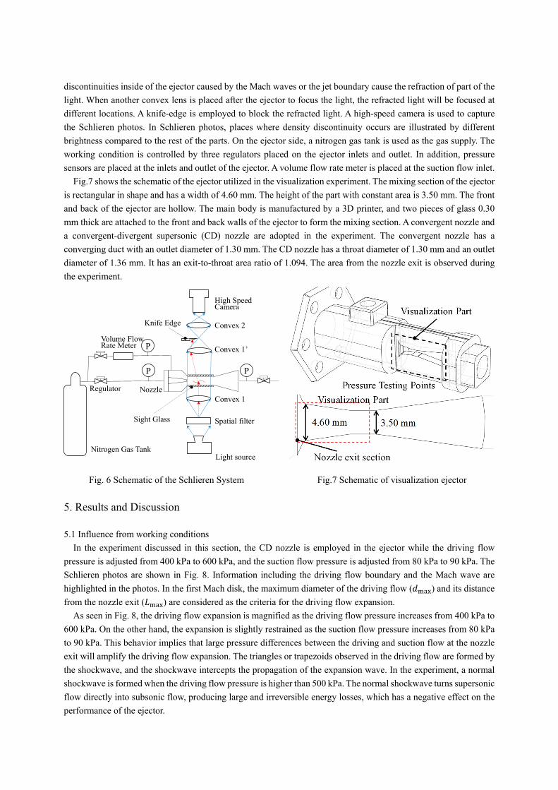
discontinuities inside of the ejector caused by the Mach waves or the jet boundary cause the refraction of part of the

light. When another convex lens is placed after the ejector to focus the light, the refracted light will be focused at

different locations. A knife-edge is employed to block the refracted light. A high-speed camera is used to capture

the Schlieren photos. In Schlieren photos, places where density discontinuity occurs are illustrated by different

brightness compared to the rest of the parts. On the ejector side, a nitrogen gas tank is used as the gas supply. The

working condition is controlled by three regulators placed on the ejector inlets and outlet. In addition, pressure

sensors are placed at the inlets and outlet of the ejector. A volume flow rate meter is placed at the suction flow inlet.

Fig.7 shows the schematic of the ejector utilized in the visualization experiment. The mixing section of the ejector

is rectangular in shape and has a width of 4.60 mm. The height of the part with constant area is 3.50 mm. The front

and back of the ejector are hollow. The main body is manufactured by a 3D printer, and two pieces of glass 0.30

mm thick are attached to the front and back walls of the ejector to form the mixing section. A convergent nozzle and

a convergent-divergent supersonic (CD) nozzle are adopted in the experiment. The convergent nozzle has a

converging duct with an outlet diameter of 1.30 mm. The CD nozzle has a throat diameter of 1.30 mm and an outlet

diameter of 1.36 mm. It has an exit-to-throat area ratio of 1.094. The area from the nozzle exit is observed during

the experiment.

Fig. 6 Schematic of the Schlieren System

Fig.7 Schematic of visualization ejector

5. Results and Discussion

5.1 Influence from working conditions

In the experiment discussed in this section, the CD nozzle is employed in the ejector while the driving flow

pressure is adjusted from 400 kPa to 600 kPa, and the suction flow pressure is adjusted from 80 kPa to 90 kPa. The

Schlieren photos are shown in Fig. 8. Information including the driving flow boundary and the Mach wave are

highlighted in the photos. In the first Mach disk, the maximum diameter of the driving flow ( ) and its distance

from the nozzle exit ( ) are considered as the criteria for the driving flow expansion.

As seen in Fig. 8, the driving flow expansion is magnified as the driving flow pressure increases from 400 kPa to

600 kPa. On the other hand, the expansion is slightly restrained as the suction flow pressure increases from 80 kPa

to 90 kPa. This behavior implies that large pressure differences between the driving and suction flow at the nozzle

exit will amplify the driving flow expansion. The triangles or trapezoids observed in the driving flow are formed by

the shockwave, and the shockwave intercepts the propagation of the expansion wave. In the experiment, a normal

shockwave is formed when the driving flow pressure is higher than 500 kPa. The normal shockwave turns supersonic

flow directly into subsonic flow, producing large and irreversible energy losses, which has a negative effect on the

performance of the ejector.

Nozzle

Sight Glass

Convex 1

Convex 1’

Convex 2Knife Edge

Spatial filter

Light source

High SpeedCamera

P

P

P

Volume Flow Rate Meter

Nitrogen Gas Tank

Regulator

In addition, are obtained from the MOC model and are compared with the measured values from the

Schlieren photos in Fig. 9. During the simulation, the grid number is increased until the value is independent

of the grid number. From Fig. 9 (a), it can be seen that the simulation results from the MOC model agree well with

the measured values. In Fig. 9 (b), increases along with , since u in the flow field is much larger than v

in the analysis. The grid number needed for a gradually changing is much larger than , and the results

of are not completely gradual. In this study, is considered as the main criteria for the evaluation,

therefore the grid number is not further increased for .

,

(kPa) , (kPa)

400 500 600

80

85

90

Fig. 8 Schlieren pictures under various driving and suction pressures

(a) Maximum driving flow diameter

(b) Distance of the surface from the nozzle exit

Fig. 9 Comparison between the MOC simulation results and the measured dimensions from the Schlieren Photos

5.2 Influence of nozzle structures

The Schlieren photos of the CD and convergent nozzles are compared in Fig. 10. The driving flow pressure is

500 kPa and the suction flow pressure is adjusted from 80 kPa to 90 kPa. Because the outflow pressure from a

convergent nozzle is higher than the outflow from a CD nozzle, a stronger expansion occurs in the convergent nozzle.

The first Mach disk from the convergent nozzle is shorter and wider than the Mach disk from the CD nozzle. Fig.

11 shows a and entrainment ratio comparison between the different nozzles. From Fig. 11 (b), it can be seen

2.1

2.0

1.9

1.8

1.7

1.6

1.5

d max

(m

m)

9590858075

Suction Pressure (kPa)

400 kPa 500 kPa 600 kPa Simulation Results

2.0

1.8

1.6

1.4

1.2

Lm

ax (

mm

)

9590858075Suction Pressure (MPa)

400 kPa 500 kPa 600 kPa Simulation Results

that the CD nozzle achieves higher performance. The results imply that appropriate expansion of the driving flow

benefits the ejector performance. However, vertical shockwaves still occur in the driving flow from both nozzles,

which means that the nozzle structure is yet not optimal in this experiment.

,

(kPa)

Types

Convergent-divergent nozzle Convergent nozzle

80

85

90

Fig. 10 Comparison between the convergent-divergent and convergent nozzle when the driving pressure is 500

kPa

(a) Maximum diameter of the driving flow

(b) Entrainment Ration comparison

Fig. 11 Comparison between the convergent-divergent nozzle and the convergent nozzle

5.3 Discussion of appropriate nozzle design

In this section, the influence of nozzle structure on the driving flow expansion is discussed based on the MOC

model. When the driving and suction flow pressures are set to 500 kPa and 80 kPa by adjusting the nozzle exit

diameter ( ), the dimensionless / results are obtained by the MOC model. These results are presented in

Fig. 12 (a). The simulation results are also compared with the isentropic expansion model given by Eq. (4), (5).

From the figure, decreases as the nozzle exit diameter increases. When the driving flow pressure at the nozzle

exit is equal to the ambient pressure, the driving flow reaches optimal condition. This behavior implies that

appropriate nozzle structure can restrain the effects of a Mach wave. If the nozzle exit diameter increases further,

an over-expanded condition occurs with an oblique shockwave. As shown in Fig. 12 (b), / increases when

the nozzle exit diameter increases. The isentropic model given by Eq. (4), (5) cannot predict the value.

2.0

1.9

1.8

1.7

1.6

d max

(m

m)

9590858075Suction Pressure (kPa)

Convergent-Divergent nozzle Convergent nozzle Simulation Results (CD) Simulation Results (C)

2.0

1.5

1.0

0.5

Ent

ranm

ent R

atio

9590858075Suction Pressure (kPa)

Convergent nozzle Convergent-divergent nozzle

(a) Dimensionless maximum driving flow diameter

(b) Dimensionless distance of the surface

Fig. 12. Simulation Results obtained by the MOC model on nozzle structures

Fig. 13 shows the simulation results from the MOC model of the driving flow boundary with two different CD

nozzle structures. The different CD nozzle structures are marked as A and B. The simulation is conducted when the

driving and suction flow pressures are 500 kPa and 80 kPa. Nozzle A is the nozzle adopted in the experiment, with

an exit-to-throat ratio of 1.094. Nozzle B is an optimized CD nozzle with an exit-to-throat ratio of 1.475. In the

figure, the boundary and expansion fan are illustrated, while the ejector wall and the grid in the driving flow regime

are omitted. By adjusting the throat-to-exit ratio of the ejector, the driving flow pressure at the nozzle exit could be

adjusted to equal the ambient pressure.

Fig. 13 Simulation results from the MOC for different nozzle exit diameters ( )

5.4 The driving flow expansion in the off-design condition

Fig. 14 (a) and (b) show the and of nozzle A and B under off-design working conditions. As the

driving flow pressure increases, the deviation between the isentropic expansion model and the MOC model increases.

This behavior implies that it is necessary to consider the Mach wave when the ejector is operated under off-design

conditions. From the figures, the larger exit diameter in nozzle B always creates more appropriate driving flow

boundary development compared to nozzle A. This means that appropriate nozzle structure design can minimize the

influence of the expansion waves.

1.5

1.4

1.3

1.2

1.1

d max

/dt

1.21.11.0de/dt

MOC simulation results Isentropic expansion fitting

shockwaves occur

Convergent Nozzle

1.4

1.3

1.2

1.1

1.0

Lm

ax/d

t

1.201.151.101.051.00de/dt

MOC simulation results fitting

shockwaves occur

Convergent Nozzle

1.0

0.8

0.6

0.4

0.2

0.03210

Unit: mm

Unit: mm Driving flow boundary

Nozzle exit

1.77 mm

mm

A

B

80 kPa80 kPa

80 kPa

1670 kPa

mm

mm

Fig. 14 Driving flow boundary prediction by the MOC when pressure changes

6. Conclusions In this research, experimental and numerical investigations on driving flow inside the ejector were conducted,

and the main conclusions are listed as follows:

1. The Method of Characteristics is applied as the numerical approach to predict the driving flow boundary

development inside the ejector in the under-expanded condition. The influence of expansion waves at the nozzle

exit was considered.

2. The numerical simulation results were validated by visualization experiments conducted using the Schlieren

optical system. The results show good agreement between the MOC simulation results and the measured values

from the experiment.

3. The values for and are affected by the nozzle structure. The expansion waves from the nozzle

exit strengthen the driving flow expansion, which creates a negative effect on ejector performance. However, with

an appropriate nozzle design, the performance of the ejector can be enhanced.

4. Under the off-design condition, deviates from the predicted value according to the isentropic expansion

equations. It is necessary to consider the influence of Mach wave on the ejector performance when an ejector is

applied in a refrigeration system with an unstable heat source.

Acknowledgement This work is partly financially supported by the Japan Science and Technology Agency (JST) under the project

“Research and Development to Find Solutions to Environmental and Energy Issues in Urban Areas”

References [1] S. Elbel, N. Lawrence, Review of recent developments in advanced ejector technology, International Journal of

Refrigeration 62 (2016) 1-18.

[2] M.T. Zegenhagen, F. Ziegler, 2015. Feasibility analysis of an exhaust gas waste heat driven jet-ejector cooling

system for charge air cooling of turbocharged gasoline engines, Applied Energy 160 (2015) 221-230.

[3] J. Yan, W.J. Cai, L. Chen, Y.Z. Li, Experimental study on performance of a hybrid ejector-vapor compression

cycle, Energy Conversion and Management 113 (2016) 36-43.

[4] S. Elbel, P. Hrnjak, Experimental validation of a prototype ejector designed to reduce throttling losses

encountered in transcritical R744 system operation, International Journal of Refrigeration 31 (3) (2008) 411-422.

[5] J.M. Abdulateef, K. Sopian, M.A. Alghoul, M.Y. Sulaiman, Review on solar-driven ejector refrigeration

technologies, Renewable and Sustainable Energy Reviews 13 (6-7) (2009) 1338-1349.

[6] B.J. Huang, W.Z. Ton, C.C. Wu, H.W. Ko, H.S Chang, H.Y. Hsu, J.H. Liu, J.H. Wu, R.H. Yen, Performance test

of solar-assisted ejector cooling system, International Journal of Refrigeration 39 (2014) 172-185.

1.7

1.6

1.5

1.4

1.3

1.2

1.1

d max

/dt

0.700.650.600.550.50Driving Flow Pressure (MPa)

Nozzle a Nozzle b isentropic expansion

1.6

1.5

1.4

1.3

1.2

1.1

Lm

ax/d

t

0.700.650.600.550.50Driving Flow Pressure (MPa)

Nozzle a Nozzle b

[7] B. Gila, J. Kasperskia, Performance analysis of a solar-powered ejector air conditioning cycle with heavier

hydrocarbons as refrigerants, Energy Procedia 57 (2013) 2619-2628.

[8] L. Zhu, J.L. Yu, M.L. Zhou, X. Wang, Performance analysis of a novel dual-nozzle ejector enhanced cycle for

solar assisted air-source heat pump systems, Renewable Energy 63 (2014) 735-740.

[9] M. Dennis, T. Cochrane, A. Marina, A prescription for primary nozzle diameters for solar driven ejectors, Solar

Energy 115 (2015) 405-412.

[10] D. Butrymowicz, K._Smierciew, J. Karwacki, J. Gagan, Experimental investigations of low-temperature driven

ejection refrigeration cycle operating with isobutene, International journal of refrigeration 39 (2014) 196-209.

[11] J.H. Keenan, E.P. Neumann, F. Lustwerk, 1950. An investigation of ejector design by analysis and experiment,

Journal of Applied Mechanics (1950) 299-309.

[12] J.T. Munday, D.F. Bugster, A new theory applied to steam jet refrigeration, Industrial and Engineering

Chemistry Process Design and Development 16 (4) (1977) 442-449.

[13] B.J. Huang, J.M. Chang, C.P. Wang, V.A. Petrenko, A 1-D analysis of ejector performance, International Journal

of Refrigeration 22 (1999) 354-364.

[14] I.W. Eames, S. Aphornratana, H. Haider, A theoretical and experimental study of a small-scale steam jet

refrigerator, International Journal of Refrigeration 18 (6) (1995) 378-386.

[15] B.J. Huang, C.B. Jiang, F.L. Hu, Ejector performance characteristics and design analysis of jet refrigeration

system, Journal of Engineering for Gas Turbines and Power 107 (3) (1985) 792-802.

[16] S.K. Chou, P.R. Yang, C. Yap, Maximum mass flow ratio due to secondary flow choking in an ejector

refrigeration system, International Journal of Refrigeration 24 (6) (2001) 486-499.

[17] K. Mohammed, G. Nicolas, S. Mikhail, Effects of design conditions and irreversibilities on the dimensions of

ejectors in refrigeration systems, Applied Energy 179 (2016) 1020–1031.

[18] Y.H. Zhu, W.J. Cai, C.Y. Wen, Y.Z. Li, Shock circle model for ejector performance evaluation, Energy

Conversion and Management 48 (9) (2007) 2533-2541.

[19] Y.H. Zhu, Y.Z. Li, Novel ejector model for performance evaluation on both dry and wet vapors ejectors,

International Journal of Refrigeration 32 (1) (2009) 21-31.

[20] H. El Dessouky, H. Ettouney, I. Alatiqi, G. Al Nuwaibit, Evaluation of steam jet ejectors, Chemical Engineering

and Processing: Process Intensification 41 (6) (2002) 551-561.

[21] S.J Chen, G.M. Chen, L.Y. Fang, An experimental study and 1-D analysis of an ejector with a movable primary

nozzle that operates with R236fa, International journal of refrigeration 60 (2015) 19-25.

[22] J.G. del Valle, J.M.S. Jabardo, F.C. Ruiz, S.J.A. J.S.J. Alonso, A one dimensional model for the determination

of an ejector entrainment ratio, International Journal of Refrigeration 35 (4) (2012) 772-784.

[23] J.Y. Chen, H. Havtun, B. Palm, Investigation of ejector in refrigeration systems: optimum performance

evaluation and ejector area ratios perspectives, Applied Thermal Engineering 64 (1-2) (2014) 182-191.

[24]. K. Matsuo, K. Sasaguchi, Y. Kiyotoki, H. Mochizuki, Investigation of supersonic air ejectors (Part 2, effects

of throat-area-ratio on ejector performance), Bulletin of the Japan Society of Mechanical Engineers 25 (210) (1982)

1898-1905.

[25] D.A. Pounds, J.M. Dong, P. Cheng, H.B. Ma, Experimental investigation and theoretical analysis of an ejector

refrigeration system, International Journal of Thermal Sciences 67 (2013) 200-209.

[26] D. Butrymowicz, K. Smierciew, J. Karwacki, Investigation of internal heat transfer in ejection refrigeration

systems, International Journal of Refrigeration 40 (2014) 131-139.

[27] W.N. Fu, Y.X. Li, Z.L. Liu, H.Q. Wu, T.R Wu, Numerical study for the influences of primary nozzle on steam

ejector performance, Applied Thermal Engineering 106 (2016) 1148-1156.

[28] N.B. Sag, H.K. Ersoy, Experimental investigation on motive nozzle throat diameter for an ejector expansion

refrigeration system, Energy Conversion and Management 124 (2016) 1-12.

[29] Y.H. Zhu, P.X. Jiang, Experimental and numerical investigation of the effect of shock wave characteristics on

the ejector performance, International Journal of Refrigeration 40 (2014) 31-42.

[30] Y.H. Zhu, P.X. Jiang, Experimental and analytical studies on the shock wave length in convergent and

convergent–divergent nozzle ejectors, Energy Conversion and Management 88 (2014) 907-914.

[31] J. Gagan, K. Smierciewa, D. Butrymowicz, J. Karwacki, Comparative study of turbulence models in application

to gas ejectors, International Journal of Thermal Sciences 78 (2014) 9-15.

[32] A. Bouhanguel, P. Desevaux, E. Gavignet, Flow visualization in supersonic ejectors using laser tomography

techniques, International Journal of Refrigeration 34 (7) (2011) 1633-1640.

[33] A.B. Little, S. Garimella, Shadowgraph visualization of condensing R134a flow through ejectors, International

Journal of Refrigeration 68 (2016) 118-129.

[34] A.L. Addy, Effects of axisymmetric sonic nozzle geometry on Mach disk characteristics, the American Institute

of Aeronautics and Astronautics Journal 19 (1) (1981) 121-122.

[35] A.J. Ruggles, I.W. Ekoto, Experimental investigation of nozzle aspect ratio effects on under expanded hydrogen

jet release characteristics, International Journal of Hydrogen energy 39 (35) 2014 20331-20338.

[36] A.L. Addy, W.L. Chow, On the starting characteristics of supersonic ejector systems, Journal of Basic

Engineering 86 (4) (1964) 861-868.

[37] M.J. Zucrow, J.D. Hoffman, Gas Dynamics. John Wiley & Sons, New York, 1976, chap. 12-16.