INVESTIGATION OF SHIP-BANK, SHIP-BOTTOM AND SHIP-SHIP INTERACTIONS BY USING POTENTIAL FLOW METHOD Z-M Yuan and A Incecik, Department of Naval Architecture, Ocean and Marine Engineering, University of Strathclyde, UK SUMMARY The authors were inspired by the benchmark model test data in MASHCON [1, 2] and carried out some numerical stud-ies on ship-bank, ship-bottom and ship-ship interactions based on potential flow method in the last few years. In the confined waterways, many researchers question the applicability of the classical potential flow method. The main objec-tive of the present paper is to present some validations of the 3D boundary element method (BEM) against the model test data to exam the feasibility of the potential method in predicting the hydrodynamic behaviour of the ships in con-fined water. The methodology used in the present paper is a 3D boundary element method based on Rankine type Green function. The numerical simulation is based on the in-house developed multi-body hydrodynamic interaction program MHydro. We calculate the wave elevations and forces (or moments) when the ship is manoeuvring in shallow and nar-row channel, or when the two ships is travelling side by side or crossing each other. These calculations are compared with the benchmark test data, as well as the published CFD results. Generally, the agreement between the present calcu-lations and model test and CFD results are satisfactory, which indicates that the potential flow method and developed program are still capable to predict the hydrodynamic interaction involved in ship-bank, ship-bottom and ship-ship prob-lem. 1 INTRODUCTION Ships manoeuvring in confined waterways is continuous-ly a topic with both academic and practical interests. As the water depth becomes small, the fluid is compressed to pass through the bottom of the vessel with larger velocity than the fluid velocity in deep water. The change of the fluid velocity could modify the pressure distribution. The negative pressure distributed on the bottom of the vessel could induce a very large suction force, which attracts the ship to sink towards the bottom of the waterway. Mean-while, the pressure distribution on the bow of the ship is different from that on the stern, which leads to the wave-making resistance and pitch moment. When the water depth becomes very small, or the forward speed increas-es, the wave-making resistance, sinkage and trim can achieve a very large value. As the resistance increases, the ship’s speed loss is inevitable. Meanwhile, due to the large sinkage and trim, the advancing ship would have the risk of grounding. Moreover, if the bank effect is taken into consideration, the shallow water problem be-comes even worse. Due to narrow gap between the bank, bottom and ship, the fluid velocity could be very large. If the banks are not symmetrical, the fluid velocity in the portside and starboard of the ship will be different, which could result in different pressure distribution, and hence leads to a suction force attracting the vessel moving to-wards the bank. Due to the non-symmetrical pressure distribution, there also exist a yaw moment which makes the ship deviate from its original course and causes the collision. For these reasons, the ships manoeuvring in shallow and narrow channel has attracted extensive inter-ests from the researchers. In order to estimate the ship-bank, ship-bottom and ship-ship interactions, the most reliable approach is by exper-imental measurement. The experimental method is ex-

tremely critical in the early years when the computer is not capable to conduct large amount of calculation. The only reliable way to predict hydrodynamic interactions relies on the model test due to the complexity of the ge-ometry of the 3D ships. The numerical method is only available when the computers are capable to solve the very large matrix. But the early version of the numerical programs to predict the hydrodynamic problem is mainly based on 2D method, or so-called strip theory. Beck et al. [3], Tuck [4-6], Newman and Tuck [7], Yaung [8] and Gourlay’s [9] proposed approaches based on the slender ship assumption. The limitation of this 2D method is very obvious. The predictions are not accurate due to the 3D effects. And also, it cannot estimate the wave-making resistance due to the assumption that the x- component of the normal vector is small on the whole body surface including bow and stern areas. In order to predict the hydrodynamic interactions accurately, the 3D potential flow method has been used nowadays, which benefits from the improvement of the computer capacity. From the published results and validations [10, 11], it can be found that the 3D potential flow method can general provide a satisfactory estimation. However, the publica-tions of using 3D potential flow method to investigate the confined water problem are still quite limited. One of the reason is the lack of the validations due to the limited model test data. The complexity of free surface condition is another reason which prevents it from being widely used. In some publications, the free surface is treated as a rigid wall. This will of course affect the accuracy of the calculations, since the wave elevation on the free surface in confined waterways could be much larger than that in open water. The limitation of the potential method lies in the assumption of ideal flow, which neglects the viscus effects. That is the reason why many researchers are still not confident about the potential flow method and doubt its reliability in confined water calculations. From this

4th MASHCON, Hamburg - Uliczka et al. (eds) - © 2016 Bundesanstalt für Wasserbau ISBN 978-3-939230-38-0 (Online) DOI: 10.18451/978-3-939230-38-0_11

83

point of view, the CFD method seems to be the perfect method to solve the ship-bank, ship-bottom and ship-ship problem. It is true that CFD programs are capable to investigate many complex hydrodynamic problems. But it is also a fact that CFD programs require highly on the computational power. Even through there are some suc-cessful examples of using CFD programs to predict the hydrodynamic problems involved in the confined water-ways [12, 13], the large amount of computational time is still a problem which prevents it from being widely used in the practice. In order to carry out parameter studies to find out the factors which determines the hydrodynamics in confined waterways, potential flow theory is still an effective method due to its acceptable calculation time. Before extending potential flow method to predict the ship-bank, ship-bottom and ship-ship problems, a rigorous valida-tion should be conducted to verify its reliability. The main objective of the present paper is to present some validations of the 3D boundary element method (BEM) against the model test data to exam the feasibility of the potential method in predicting the hydrodynamics in-volved in ship-bank, ship-bottom and ship-ship problems. Since 2009, the International Conference on Ship Manoeuvring in Shallow and Confined Water has suc-cessfully attracted the researchers to deal with the hydro-dynamics involved in confined waterways. And during these conferences, Ghent University in cooperation with the Flanders Hydraulics Research (FHR) published ex-tensive benchmark model test data related to various topics, including bank effects (Antwerp, May 2009), ship-ship interaction (Trondheim, May 2011) and ship behaviour in locks (Ghent, June 2013). Based on these model test data, the validations of applying potential flow method to predict the ship-bank, ship-bottom and ship-ship problems will be carried out in the present paper. 2 MATHEMATICAL FORMULATION 2.1 THE BOUNDARY VALUE PROBLEM OF

SHIP-BANK AND SHIP-BOTTOM PROBLEM

When a ship advances at constant speed in calm water, it will generate steady waves and induce the so-called wave-making resistance. It is assumed that the fluid is incompressible and inviscid and the flow is irrotational. A velocity potential T uxϕ ϕ= + is introduced and φ satisfies the Laplace equation 2 0ϕ∇ =

2 0ϕ∇ = in the fluid domain (1)

Following Newman [14], the nonlinear dynamic free-surface condition on the disturbed free surface can be expressed as

22 21 0, 2

u gx x y zϕ ϕ ϕ ϕ z

∂ ∂ ∂ ∂ + + + + = ∂ ∂ ∂ ∂ ( , )on z x yz= (2)

The kinematic free-surface condition is

0, ( , )u on z x yx z y y x xz ϕ ϕ z ϕ z z∂ ∂ ∂ ∂ ∂ ∂

− + + = =∂ ∂ ∂ ∂ ∂ ∂

(3)

The first approximation is based on the linear free surface conditions on the undisturbed water surface. By neglect-ing the nonlinear terms in Eq. (2) and (3), we can obtain the linear classic free surface boundary condition

22

2 0u gzx

ϕ ϕ∂ ∂+ =

∂∂, on the undisturbed free surface

(4)

For the ship-to-ship with same forward speed problem, the body surface boundary condition can be written as

1u nnϕ∂

= ⋅∂

, on the wetted body surface (5)

where 1 2 3( , , )n n n=n is the unit normal vector inward on the wetted body surface of Ship_a and Ship_b. The boundary condition on the sea bottom and side walls can be expressed as

0nϕ∂

=∂

, on z = -h and side walls (6)

Besides, a radiation condition is imposed on the control surface to ensure that the waves vanish upstream of the disturbance.

2.2 THE BOUNDARY VALUE PROBLEM OF SHIP-SHIP PROBLEM

In order to deal with the different forward speeds, we propose a new uncoupled method. The potential φ can be divided into two components

a bϕ ϕ ϕ= + (7)

φa is the potential produced by the case that Ship_a is moving with ua while Ship_b is stationary. According to the linear theory, it satisfies the Laplace equation. The boundary value problem for φa can be written as

2

1

22

2

0, in the fluid domain

, on wet body surface of Ship_a

0, on wet body surface of Ship_b

0, on undisturbed free surface

0, on sea bottom and side wa

a

aa

a

a aa

a

u nn

n

u gzx

n

ϕϕ

ϕ

ϕ ϕ

ϕ

∇ =

∂= ⋅

∂∂

=∂

∂ ∂+ =

∂∂∂

=∂

lls

(8)

Similarly, the φb is defined as the potential produced by the case that Ship_b is moving with ub while Ship_a is stationary. The boundary value problem for φb can be written as

84

2

1

22

2

0, in the fluid domain

, on wet body surface of Ship_b

0, on wet body surface of Ship_a

0, on undisturbed free surface

0, on sea bottom and side wa

b

bb

b

b bb

b

u nn

n

u gzx

n

ϕϕ

ϕ

ϕ ϕ

ϕ

∇ =

∂= ⋅

∂∂

=∂

∂ ∂+ =

∂∂∂

=∂

lls

(9)

φa and φb can be obtained by solving the boundary value problem in Eq. (8) and (9). The details about how to discretise the boundaries numerically by using the 3D Rankine source method can be found in Yuan et al. [15]. The same procedure will be applied in the present study.

3 VALIDATIONS AND DISCUSSIONS

The above theory is applied in our in-house developed 3D BEM program MHydro to investigate the ship-bank, ship-bottom and ship-ship problems. The convergence study for MHydro can be found in Yuan et al. [16].

3.1 VALIDATION OF SHIP-BANK INTERACTION

3.1 (a) Ship model and test matrix

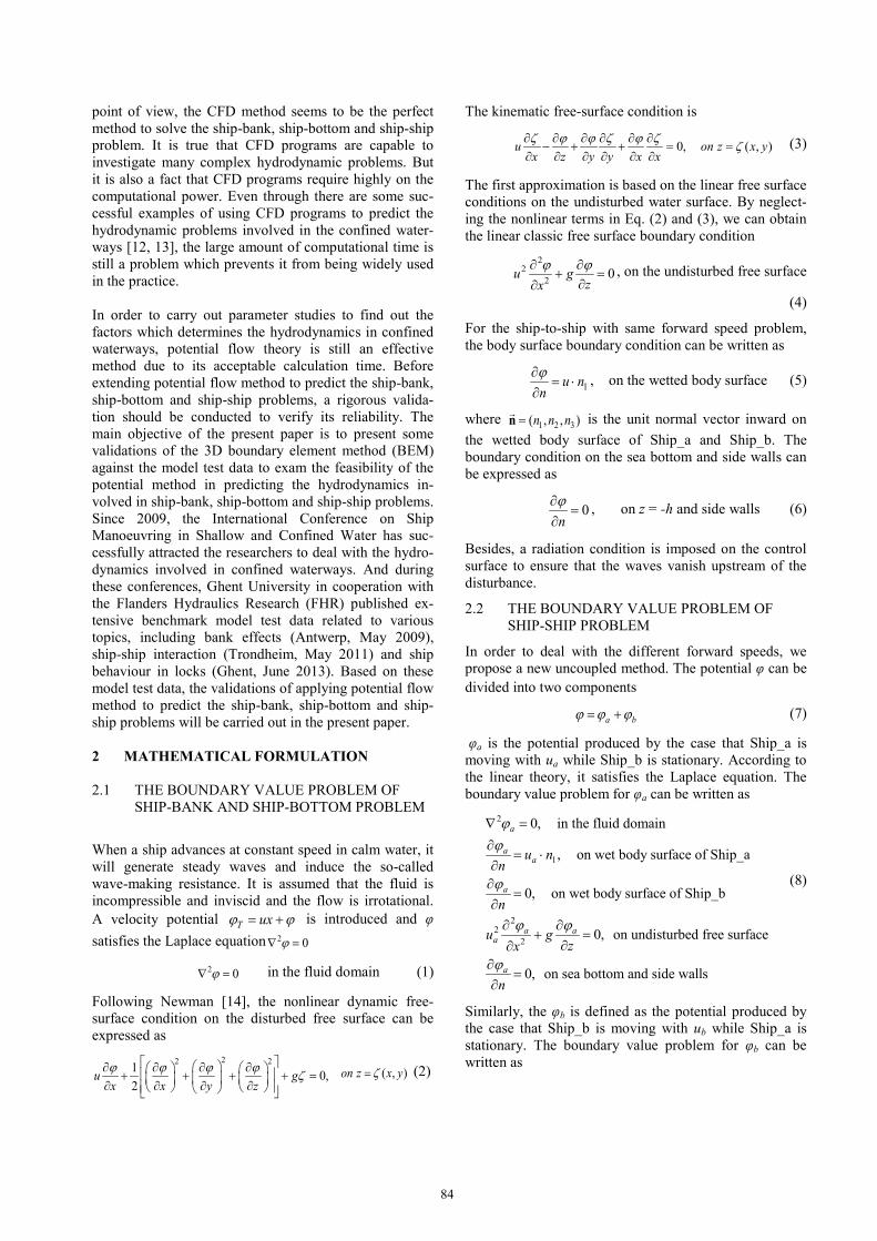
The ship model used in ship-bank and ship-bottom prob-lem is a very large crude oil carrier (referred as KVLCC2 hereafter). The main particulars of the KVLCC2, de-signed by MOERI, in model scale with scale factor 1/75 are shown in Table 1. The model tests of bank and bot-tom effects are conducted at Flanders Hydraulics Re-search (FHR), and the measurement data, as well as the CFD results used in the present paper is published by Hoydonck, et al. [17]. The towing tank at FHR is 88 m (length) × 7 m (breadth) × 0.5 m (depth). The towing tank is equipped with a double bank configuration along the full length of the tank. An overview of the towing tank with banks is shown in Figure 1.

Table 1. Main particulars of KVLCC2 (model scale) Length (L) (m) 4.2667 Breadth (B) (m) 0.773 Draft Amidships (T) (m) 0.2776 Longitudinal CoG ( XG) (m) 0.1449 Vertical CoG (KG) (m) 0.2776 Displacement (m3) 0.741 Block coefficient 0.8098

Figure 1. Cross section of the tank geometry, where dsb is the distance between the ship and vertical bank, d is the water depth and tan(θ) = 1 / 4.

In the present study, we only present the results of the ship model without consideration of propulsion. ) is 0.055. Table 2 lists the test matrix of the cases without propul-sion. Case 1- Case 3 has the same water depth (d), while the distance between the ship and the vertical wall (dsb) is different. Therefore, this set of cases are used to represent the ship-bank interaction. Case 3- Case 5 has the same dsb, while the water depth is different. Therefore, this set of cases are used to represent the ship-bottom interaction. In Case 1- Case 5, the Froude number Fn ( /nF u gL= ) is 0.055.

Table 2. Test matrix of the cases without propulsion.

Test case dsb (m) dsb / B d (m) d / T

Case 1 0.5175 0.67 0.3744 1.35 Case 2 0.5866 0.76 0.3744 1.35 Case 3 0.9731 1.26 0.3744 1.35 Case 4 0.9731 1.26 0.416 1.5 Case 5 0.9731 1.26 0.3051 1.1

Figure 2. Mesh distribution on wet body surface of KVLCC2. There are 8,080 panels distrib-uted on the body surface.

Figure 3. The coordinate system and panel distribu-tion on the computational domain of Case 1. There are 27,060 panels distributed onthe entire computational domain: 8,080 onthe body surface of body surface, 17,700 onthe free surface, and 1280 on the side walls.The computational domain is truncated atL upstream and 2L downstream. The con-tour of this figure illustrates the wave ele-vations on the free surface of Case 1.

85

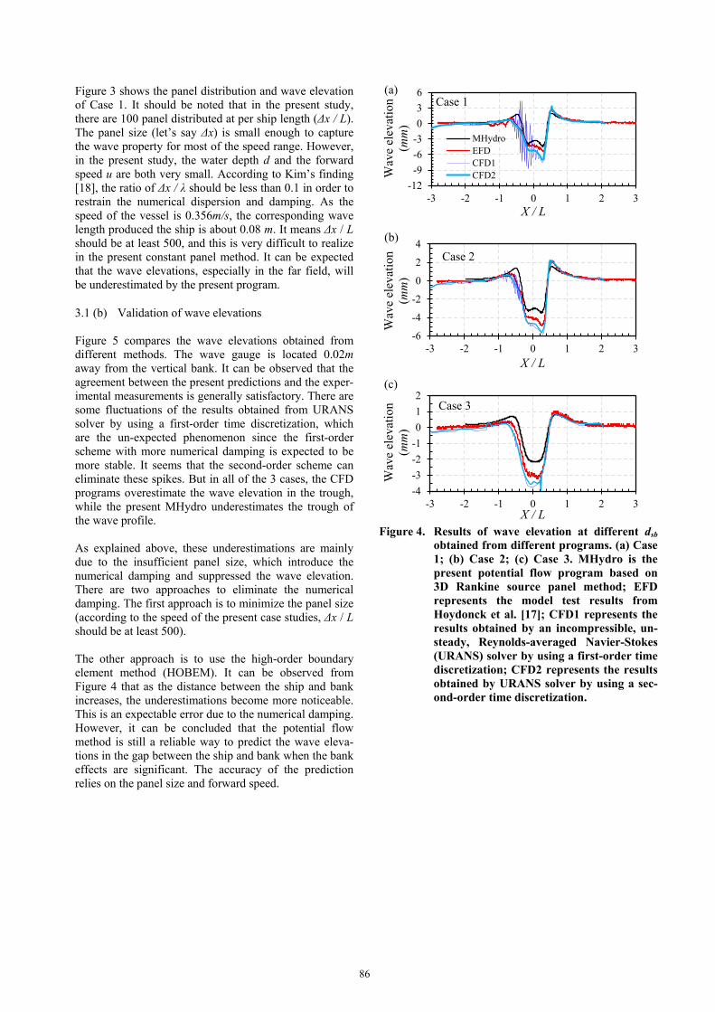
Figure 3 shows the panel distribution and wave elevation of Case 1. It should be noted that in the present study, there are 100 panel distributed at per ship length (Δx / L). The panel size (let’s say Δx) is small enough to capture the wave property for most of the speed range. However, in the present study, the water depth d and the forward speed u are both very small. According to Kim’s finding [18], the ratio of Δx / λ should be less than 0.1 in order to restrain the numerical dispersion and damping. As the speed of the vessel is 0.356m/s, the corresponding wave length produced the ship is about 0.08 m. It means Δx / L should be at least 500, and this is very difficult to realize in the present constant panel method. It can be expected that the wave elevations, especially in the far field, will be underestimated by the present program.

3.1 (b) Validation of wave elevations

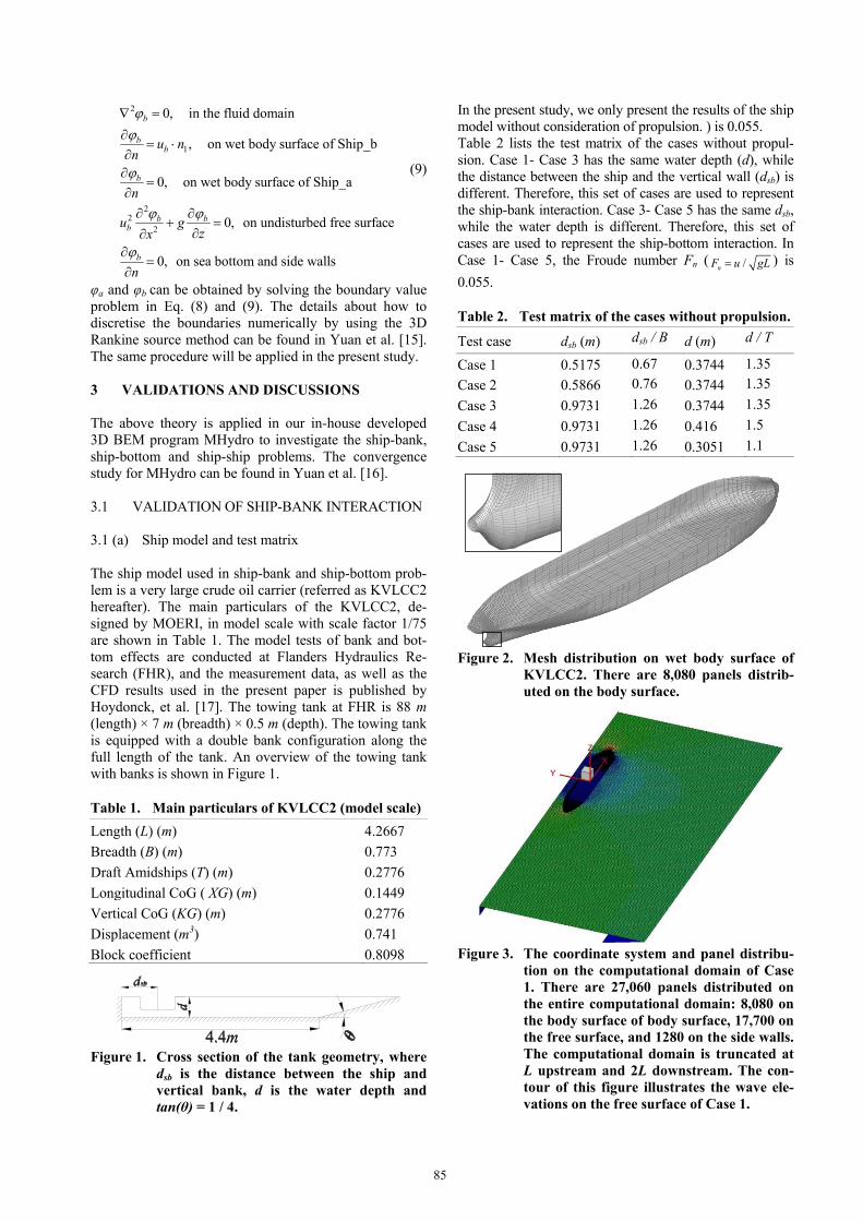
Figure 5 compares the wave elevations obtained from different methods. The wave gauge is located 0.02m away from the vertical bank. It can be observed that the agreement between the present predictions and the exper-imental measurements is generally satisfactory. There are some fluctuations of the results obtained from URANS solver by using a first-order time discretization, which are the un-expected phenomenon since the first-order scheme with more numerical damping is expected to be more stable. It seems that the second-order scheme can eliminate these spikes. But in all of the 3 cases, the CFD programs overestimate the wave elevation in the trough, while the present MHydro underestimates the trough of the wave profile.

As explained above, these underestimations are mainly due to the insufficient panel size, which introduce the numerical damping and suppressed the wave elevation. There are two approaches to eliminate the numerical damping. The first approach is to minimize the panel size (according to the speed of the present case studies, Δx / L should be at least 500).

The other approach is to use the high-order boundary element method (HOBEM). It can be observed from Figure 4 that as the distance between the ship and bank increases, the underestimations become more noticeable. This is an expectable error due to the numerical damping. However, it can be concluded that the potential flow method is still a reliable way to predict the wave eleva-tions in the gap between the ship and bank when the bank effects are significant. The accuracy of the prediction relies on the panel size and forward speed.

Figure 4. Results of wave elevation at different dsb obtained from different programs. (a) Case 1; (b) Case 2; (c) Case 3. MHydro is the present potential flow program based on 3D Rankine source panel method; EFD represents the model test results from Hoydonck et al. [17]; CFD1 represents the results obtained by an incompressible, un-steady, Reynolds-averaged Navier-Stokes (URANS) solver by using a first-order time discretization; CFD2 represents the results obtained by URANS solver by using a sec-ond-order time discretization.

-12-9-6-3036

-3 -2 -1 0 1 2 3

Wav

e el

evat

ion

(mm

)

X / L

Case 1

MHydroEFDCFD1CFD2

-6

-4

-2

0

2

4

-3 -2 -1 0 1 2 3

Wav

e el

evat

ion

(mm

)

X / L

Case 2

-4-3-2-1012

-3 -2 -1 0 1 2 3

Wav

e el

evat

ion

(mm

)

X / L

Case 3

(b)

(c)

(a)

86

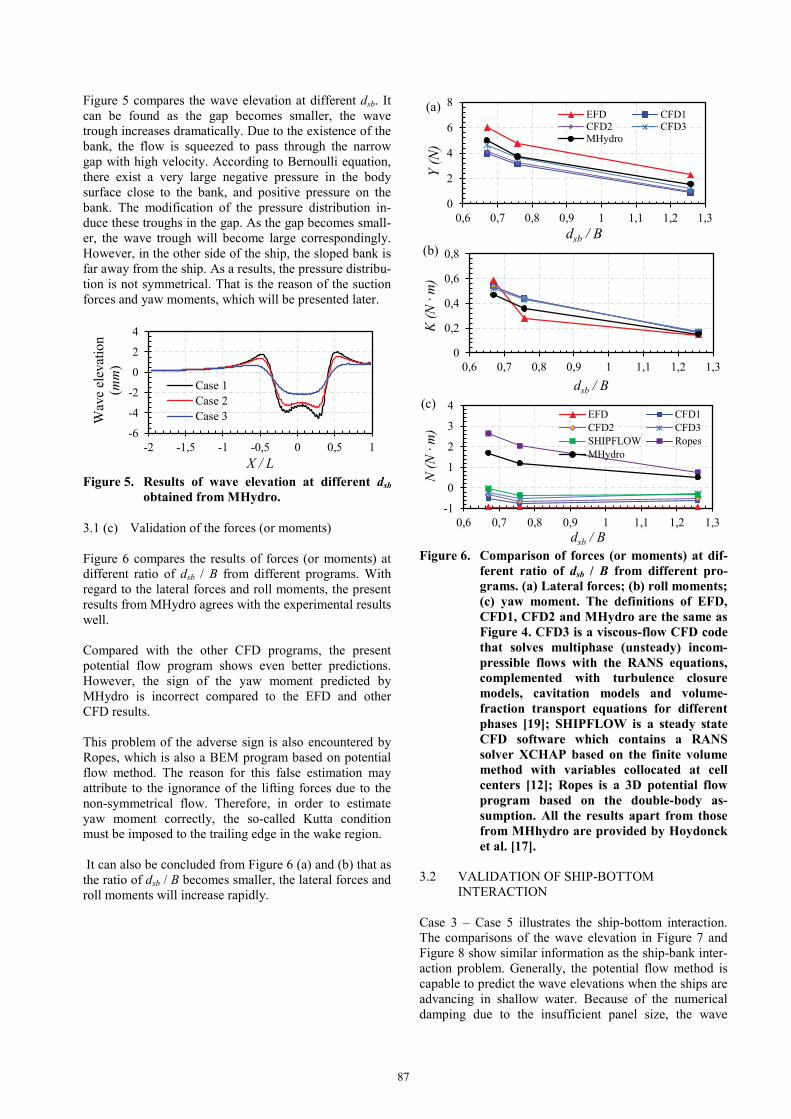
Figure 5 compares the wave elevation at different dsb. It can be found as the gap becomes smaller, the wave trough increases dramatically. Due to the existence of the bank, the flow is squeezed to pass through the narrow gap with high velocity. According to Bernoulli equation, there exist a very large negative pressure in the body surface close to the bank, and positive pressure on the bank. The modification of the pressure distribution in-duce these troughs in the gap. As the gap becomes small-er, the wave trough will become large correspondingly. However, in the other side of the ship, the sloped bank is far away from the ship. As a results, the pressure distribu-tion is not symmetrical. That is the reason of the suction forces and yaw moments, which will be presented later.

Figure 5. Results of wave elevation at different dsb

obtained from MHydro.

3.1 (c) Validation of the forces (or moments) Figure 6 compares the results of forces (or moments) at different ratio of dsb / B from different programs. With regard to the lateral forces and roll moments, the present results from MHydro agrees with the experimental results well. Compared with the other CFD programs, the present potential flow program shows even better predictions. However, the sign of the yaw moment predicted by MHydro is incorrect compared to the EFD and other CFD results. This problem of the adverse sign is also encountered by Ropes, which is also a BEM program based on potential flow method. The reason for this false estimation may attribute to the ignorance of the lifting forces due to the non-symmetrical flow. Therefore, in order to estimate yaw moment correctly, the so-called Kutta condition must be imposed to the trailing edge in the wake region. It can also be concluded from Figure 6 (a) and (b) that as the ratio of dsb / B becomes smaller, the lateral forces and roll moments will increase rapidly.

Figure 6. Comparison of forces (or moments) at dif-

ferent ratio of dsb / B from different pro-grams. (a) Lateral forces; (b) roll moments; (c) yaw moment. The definitions of EFD, CFD1, CFD2 and MHydro are the same as Figure 4. CFD3 is a viscous-flow CFD code that solves multiphase (unsteady) incom-pressible flows with the RANS equations, complemented with turbulence closure models, cavitation models and volume-fraction transport equations for different phases [19]; SHIPFLOW is a steady state CFD software which contains a RANS solver XCHAP based on the finite volume method with variables collocated at cell centers [12]; Ropes is a 3D potential flow program based on the double-body as-sumption. All the results apart from those from MHhydro are provided by Hoydonck et al. [17].

3.2 VALIDATION OF SHIP-BOTTOM

INTERACTION Case 3 – Case 5 illustrates the ship-bottom interaction. The comparisons of the wave elevation in Figure 7 and Figure 8 show similar information as the ship-bank inter-action problem. Generally, the potential flow method is capable to predict the wave elevations when the ships are advancing in shallow water. Because of the numerical damping due to the insufficient panel size, the wave

-6

-4

-2

0

2

4

-2 -1,5 -1 -0,5 0 0,5 1

Wav

e el

evat

ion

(mm

)

X / L

Case 1Case 2Case 3

0

2

4

6

8

0,6 0,7 0,8 0,9 1 1,1 1,2 1,3

Y (N

)

dsb / B

EFD CFD1CFD2 CFD3MHydro

0

0,2

0,4

0,6

0,8

0,6 0,7 0,8 0,9 1 1,1 1,2 1,3

K (N

∙ m

)

dsb / B

-1

0

1

2

3

4

0,6 0,7 0,8 0,9 1 1,1 1,2 1,3

N (N

∙ m

)

dsb / B

EFD CFD1CFD2 CFD3SHIPFLOW RopesMHydro

(c)

(a)

(b)

87

(b)

(b)

(c)

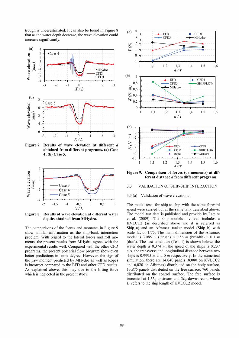
trough is underestimated. It can also be found in Figure 8 that as the water depth decrease, the wave elevation could increase significantly.

Figure 7. Results of wave elevation at different d

obtained from different programs. (a) Case 4; (b) Case 5.

Figure 8. Results of wave elevation at different water

depths obtained from MHydro. The comparisons of the forces and moments in Figure 9 show similar information as the ship-bank interaction problem. With regard to the lateral forces and roll mo-ments, the present results from MHydro agrees with the experimental results well. Compared with the other CFD programs, the present potential flow program show even better predictions in some degree. However, the sign of the yaw moment predicted by MHydro as well as Ropes is incorrect compared to the EFD and other CFD results. As explained above, this may due to the lifting force which is neglected in the present study.

Figure 9. Comparison of forces (or moments) at dif-

ferent distance d from different programs. 3.3 VALIDATION OF SHIP-SHIP INTERACTION 3.3 (a) Validation of wave elevations The model tests for ship-to-ship with the same forward speed were carried out at the same tank described above. The model test data is published and provide by Lataire et al. (2009). The ship models involved includes a KVLCC2 (as described above and it is referred as Ship_a) and an Aframax tanker model (Ship_b) with scale factor 1/75. The main dimension of the Aframax model is 3.085 m (length) × 0.56 m (breadth) × 0.1 m (draft). The test condition (Test 1) is shown below: the water depth is 0.374 m, the speed of the ships is 0.237 m/s, the transverse and longitudinal distance between two ships is 0.9995 m and 0 m respectively. In the numerical simulation, there are 14,040 panels (8,080 on KVLCC2 and 6,020 on Aframax) distributed on the body surface, 13,875 panels distributed on the free surface, 760 panels distributed on the control surface. The free surface is truncated at 1.5La upstream and 3La downstream, where La refers to the ship length of KVLCC2 model.

-4-3-2-101234

-3 -2 -1 0 1 2 3

Wav

e el

evat

ion

(mm

)

X / L

Case 4

MHydroEFDCFD1

-6

-4

-2

0

2

-3 -2 -1 0 1 2 3

Wav

e el

evat

ion

(mm

)

X / L

Case 5

-4

-2

0

2

-2 -1,5 -1 -0,5 0 0,5 1

Wav

e el

evat

ion

(mm

)

X / L

Case 3Case 4Case 5

-1

0

1

2

3

4

1 1,1 1,2 1,3 1,4 1,5 1,6

Y (N

)

d / T

EFD CFD1CFD3 MHydro

0

0,2

0,4

0,6

0,8

1

1 1,1 1,2 1,3 1,4 1,5 1,6

K (N

∙ m

)

d / T

EFD CFD1CFD3 SHIPFLOWMHydro

-10-8-6-4-202

1 1,1 1,2 1,3 1,4 1,5 1,6

N (N

∙ m

)

d / T

EFD CDF1CFD3 SHIPFLOWRopes MHydro

(a)

(a)

88

(b)

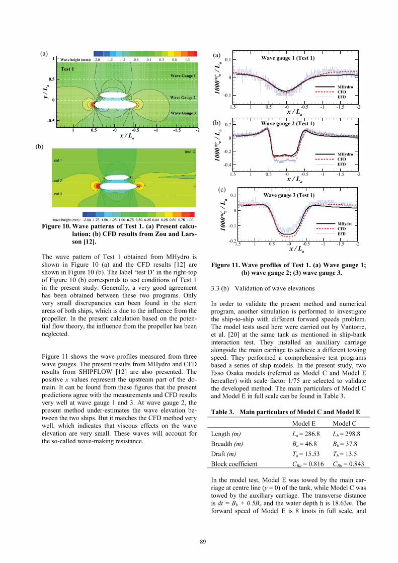
Figure 10. Wave patterns of Test 1. (a) Present calcu-

lation; (b) CFD results from Zou and Lars-son [12].

The wave pattern of Test 1 obtained from MHydro is shown in Figure 10 (a) and the CFD results [12] are shown in Figure 10 (b). The label ‘test D’ in the right-top of Figure 10 (b) corresponds to test conditions of Test 1 in the present study. Generally, a very good agreement has been obtained between these two programs. Only very small discrepancies can been found in the stern areas of both ships, which is due to the influence from the propeller. In the present calculation based on the poten-tial flow theory, the influence from the propeller has been neglected.

Figure 11 shows the wave profiles measured from three wave gauges. The present results from MHydro and CFD results from SHIPFLOW [12] are also presented. The positive x values represent the upstream part of the do-main. It can be found from these figures that the present predictions agree with the measurements and CFD results very well at wave gauge 1 and 3. At wave gauge 2, the present method under-estimates the wave elevation be-tween the two ships. But it matches the CFD method very well, which indicates that viscous effects on the wave elevation are very small. These waves will account for the so-called wave-making resistance.

Figure 11. Wave profiles of Test 1. (a) Wave gauge 1; (b) wave gauge 2; (3) wave gauge 3.

3.3 (b) Validation of wave elevations In order to validate the present method and numerical program, another simulation is performed to investigate the ship-to-ship with different forward speeds problem. The model tests used here were carried out by Vantorre, et al. [20] at the same tank as mentioned in ship-bank interaction test. They installed an auxiliary carriage alongside the main carriage to achieve a different towing speed. They performed a comprehensive test programs based a series of ship models. In the present study, two Esso Osaka models (referred as Model C and Model E hereafter) with scale factor 1/75 are selected to validate the developed method. The main particulars of Model C and Model E in full scale can be found in Table 3.

Table 3. Main particulars of Model C and Model E

Model E Model C

Length (m) La = 286.8 Lb = 298.8 Breadth (m) Ba = 46.8 Bb = 37.8 Draft (m) Ta = 15.53 Tb = 13.5 Block coefficient CBa = 0.816 CBb = 0.843

In the model test, Model E was towed by the main car-riage at centre line (y = 0) of the tank, while Model C was towed by the auxiliary carriage. The transverse distance is dt = Bb + 0.5Ba and the water depth h is 18.63m. The forward speed of Model E is 8 knots in full scale, and

x / La

y/L

a

1 0.5 -0 -0.5 -1 -1.5 -2

-0.5

0

0.5

1 Wave height (mm): -2.0 -1.5 -1.1 -0.6 -0.1 0.3 0.8 1.3

Wave Gauge 2

Wave Gauge 3

Test 1Wave Gauge 1

x / La

1000*z

/La

1.5 1 0.5 -0 -0.5 -1 -1.5 -2

-0.1

0

0.1

MHydroCFDEFD

Wave gauge 1 (Test 1)

x / La

1000*z

/La

1.5 1 0.5 -0 -0.5 -1 -1.5 -2

-0.4

-0.2

0

0.2

MHydroCFDEFD

Wave gauge 2 (Test 1)

x / La

1000*z

/La

1.5 1 0.5 -0 -0.5 -1 -1.5 -2-0.2

-0.1

0

0.1

MHydroCFDEFD

Wave gauge 3 (Test 1)

(a) (a)

(b)

(c)

(b)

89

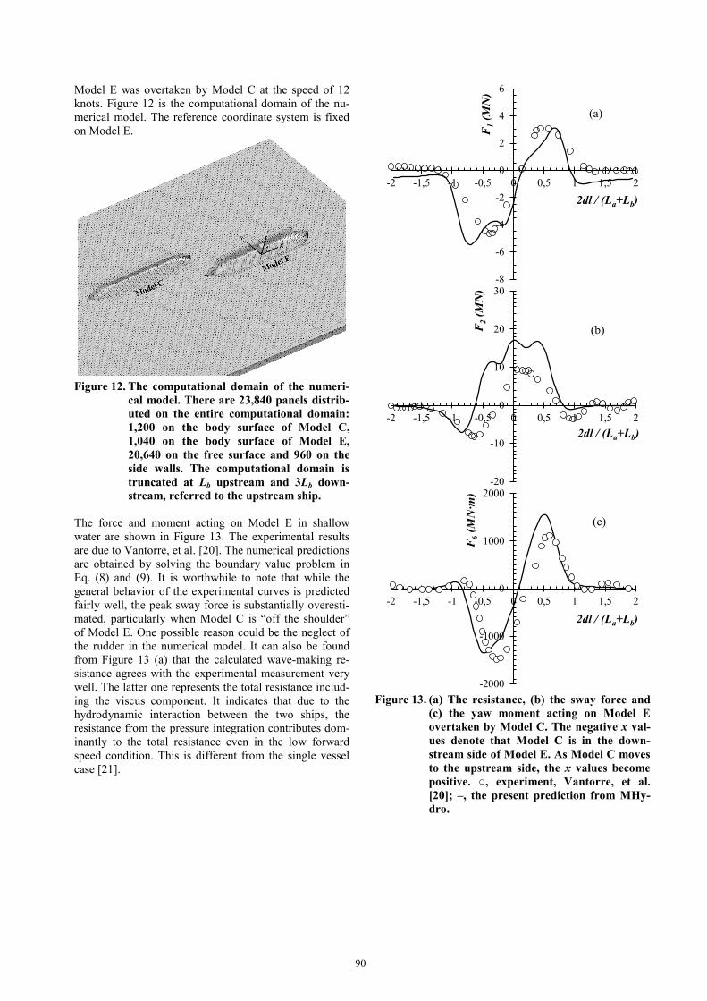
Model E was overtaken by Model C at the speed of 12 knots. Figure 12 is the computational domain of the nu-merical model. The reference coordinate system is fixed on Model E.

Figure 12. The computational domain of the numeri-

cal model. There are 23,840 panels distrib-uted on the entire computational domain: 1,200 on the body surface of Model C, 1,040 on the body surface of Model E, 20,640 on the free surface and 960 on the side walls. The computational domain is truncated at Lb upstream and 3Lb down-stream, referred to the upstream ship.

The force and moment acting on Model E in shallow water are shown in Figure 13. The experimental results are due to Vantorre, et al. [20]. The numerical predictions are obtained by solving the boundary value problem in Eq. (8) and (9). It is worthwhile to note that while the general behavior of the experimental curves is predicted fairly well, the peak sway force is substantially overesti-mated, particularly when Model C is “off the shoulder” of Model E. One possible reason could be the neglect of the rudder in the numerical model. It can also be found from Figure 13 (a) that the calculated wave-making re-sistance agrees with the experimental measurement very well. The latter one represents the total resistance includ-ing the viscus component. It indicates that due to the hydrodynamic interaction between the two ships, the resistance from the pressure integration contributes dom-inantly to the total resistance even in the low forward speed condition. This is different from the single vessel case [21].

Figure 13. (a) The resistance, (b) the sway force and

(c) the yaw moment acting on Model E overtaken by Model C. The negative x val-ues denote that Model C is in the down-stream side of Model E. As Model C moves to the upstream side, the x values become positive. ○, experiment, Vantorre, et al. [20]; –, the present prediction from MHy-dro.

-8

-6

-4

-2

0

2

4

6

-2 -1,5 -1 -0,5 0 0,5 1 1,5 2

F1 (

MN

)

2dl / (La+Lb)

(a)

-20

-10

0

10

20

30

-2 -1,5 -1 -0,5 0 0,5 1 1,5 2

F2 (

MN

)

2dl / (La+Lb)

(b)

-2000

-1000

0

1000

2000

-2 -1,5 -1 -0,5 0 0,5 1 1,5 2

F6 (

MN

∙m)

2dl / (La+Lb)

(c)

90

4 CONCLUSIONS In the present study, we present many case studies which include the problems of ship-bank, ship-bottom and ship-ship interaction. The results of the present study are cal-culated by potential flow program. Through the compari-sons to the experimental measurements and CFD calcula-tion, we can come to the following conclusions:

1) The potential flow method is a reliable way to predict the wave elevation when the bank and bottom effects are significant. The accuracy of the prediction relies on the panel size and for-ward speed. As for the very low forward speed cases, the potential flow method underestimates the wave trough due to the insufficient panel distributed on the free surface;

2) Compared with the CFD programs, the present potential flow program shows even better pre-dictions in predicting the lateral forces and roll moments in the confined waterways. However, because of the neglecting of the lifting forces due to the non-symmetrical flow, the potential flow method fails to predict the sign of the yaw moment. In order to estimate yaw moment cor-rectly, the so-called Kutta condition must be im-posed to the trailing edge in the wake region.

3) The potential flow method is able to predict the wave elevation of ship-ship problem. The forces or moments predicted by potential flow method have a good agreement with the model test re-sults.

5 ACKNOWLEDGEMENTS The work reported in this paper was performed within the project “Energy Efficient Safe Ship Operation (SHOP-ERA)” funded by the European commission under con-tract No. 605221. The authors thank Maxim Candries and Evert Lataire at Ghent University, Wim Van Hoydonck at Flanders Hydraulics Research, for support and allow-ing us to use their model test data for validations. 6 REFERENCES 1. Lataire, E., M. Vantorre, and G. Delefortrie, Captive model testing for ship to ship operations, in MARSIM 2009. 2009: Panama City, Panama. 2. Vantorre, M., G. Delefortrie, and F. Mostaert, Behaviour of ships approaching and leaving locks: Open model test data for validation purposes. Version 3_0. WL Rapporten, WL2012R815_08e. Flanders Hydraulics Research and Ghent University - Division of Maritime Technology: Antwerp, Belgium. 2012. 3. Beck, R.F., J.N. Newman, and E.O. Tuck, Hydrodynamic forces on ships in dredged channels. Journal of Ship Research, 1975. 19(3): p. 166–171.

4. Tuck, E.O., A systematic asymptotic expansion procedure for slender ships. Journal of Ship Research, 1964. 8: p. 15–23. 5. Tuck, E.O., Shallow water flows past slender bodies. Journal of Fluid Mechanics, 1966. 26: p. 81–95. 6. Tuck, E.O., Sinkage and trim in shallow water of finite width. Schiffstechnik, 1967. 14: p. 92–94. 7. Tuck, E.O. and J.N. Newman, Hydrodynamic interactions between ships, in Proceedings of 10th Symposium on Naval Hydrodynamics. 1974: Cambridge, MA, USA. p. 35-70. 8. Yeung, R.W. and W.T. Tan, Hydrodynamic interactions of ships with fixed obstacles. Journal of Ship Research, 1980. 24(1): p. 50-59. 9. Gourlay, T., Slender-body methods for predicting ship squat. Ocean Engineering, 2008. 35(2): p. 191-200. doi:10.1016/j.oceaneng.2007.09.001. 10. Yuan, Z.M., et al., Ship-to-Ship Interaction during Overtaking Operation in Shallow Water. Journal of Ship Research, 2015. 59(3): p. 172-187. doi: 10.5957/JOSR. 59.3.150004. 11. Yao, J.-x. and Z.-j. Zou, Calculation of ship squat in restricted waterways by using a 3D panel method. Journal of Hydrodynamics, Ser. B, 2010. 22(5): p. 489-494. doi: 10.1016/S1001-6058(09)60241-9. 12. Zou, L. and L. Larsson, Numerical predictions of ship-to-ship interaction in shallow water. Ocean Engineering, 2013. 72: p. 386-402. doi:10.1016/j.oceaneng.2013.06 .0 15. 13. Sakamoto, N., R.V. Wilson, and F. Stern, Reynolds-Averaged Navier-Stokes Simulations for High-Speed Wigley Hull in Deep and Shallow Water. Journal of Ship Research, 2007. 51(3): p. 187-203. 14. Newman, J.N., Linearized wave resistance, in International Seminar on Wave resistance. 1976: Tokyo. 15. Yuan, Z.M., A. Incecik, and L. Jia, A new radiation condition for ships travelling with very low forward speed. Ocean Engineering 2014. 88: p. 298-309. doi:10.1016/j.oceaneng.2014.05.019. 16. Yuan, Z.M., A. Incecik, and A. Day, Verification of a new radiation condition for two ships advancing in waves. Applied Ocean Research 48, 2014: p. 186-201. doi:10.1016/j.apor.2014.08.007. 17. Hoydonck, W.V., et al., Bank Effects for KVLCC2, in World Maritime Technology Conference. 2015: Rhode Island, USA.

91

18. Kim, Y., D.K.P. Yue, and B.S.H. Connell, Numerical dispersion and damping on steady waves with forward speed. Applied Ocean Research, 2005. 27(2): p. 107-125. doi:10.1016/j.apor.2005.11.002. 19. Vaz, G., F.A.P. Jaouen, and M. Hoekstra, Free Surface Viscous Flow Computations. Validation of URANS Code FRESCO, in 28 th International

20. Vantorre, M., E. Verzhbitskaya, and E. Laforce, Model test based formulations of ship–ship interaction forces. Ship Technology Research, 2002. 49: p. 124-141. 21. Schultz, M.P., Effects of coating roughness and biofouling on ship resistance and powering. Biofouling, 2007. 23(5-6): p. 331-41. doi:10.1080/ 089270107014619 74. 7 AUTHORS’ BIOGRAPHIES Zhi-Ming Yuan holds the current position of lecturer in hydrodynamics at University of Strathclyde. His research interests mainly lie in the theoretical and numerical anal-ysis of the hydrodynamic performance of the ship and offshore structures Atilla Incecik is a Professor of Offshore Engineering and Associate Deputy Principal at Strathclyde University. His current research includes development of dynamic load and response prediction tools for the design and installa-tion of floating offshore platforms and marine renewable energy devices; seakeeping of marine vehicles; and low carbon shipping.

92