investigation of long-term variations in stratospheric ozone through

INVESTIGATION OF LONG-TERM VARIATIONS IN

STRATOSPHERIC OZONE THROUGH THE

COMBINATION OF DIFFERENT SATELLITE OZONE

DATA SETS

A MASTER THESIS SUBMITTED TO THE INSTITUTE OF ENVIRONMENTAL PHYSICS (IUP)

By

Ebojie, Felix(Mat. No. 2196990)

IN PARTIAL FULFILLMENT OF THE REQUIREMENTS FOR THE DEGREE OF

Master of Science

POSTGRADUATE PROGRAMME ENVIRONMENTAL PHYSICS (PEP)UNIVERSITY OF BREMEN (FB1), BREMEN, GERMANY

August, 2009

SUPERVISOR: PD Dr. Christian von Savigny

REFEREE: 1. PD Dr. Annette Ladstätter-Weißenmayer 2. PD Dr. Christian von Savigny

i

Declaration

I Ebojie, Felix herewith declare that I did the written work on my own and only with the

means as indicated.

Date Signature

ii

Acknowledgements

My first thanks goes to every member of the department for their contributions in one

way or another towards the completion of this programme. Among this great minds are

Mr. Lars Jescke, the first name I got to know in this programme while back home in my

country. Further thanks goes to Mrs. Anja Gatzka an intelligent and understanding

secretary, Thiranan Sonkaew, a Phd student for helping me out at the earlier stage of this

work, and my entire lecturers for their excellent and pragmatic teachings. My sincere

appreciation goes to PD Dr. Christian von Savigny who was first my course mentor and

later became my thesis supervisor and examiner, for his support in tougher times,

teaching, patience, encouragement, guidance and understanding during this thesis work.

Special thanks to my first examiner PD. Dr. Annette Ladstätter-Weißenmayer for her

support and encouragement. I appreciate Prof Noltholt for his understanding and counsel

when I was to choose my thesis topic. Many thanks also go to Prof. Dr. John Burrows in

whose group I conducted this thesis. Thanks to my colleagues and a special thanks to my

mum, brothers and sisters for their support, love and cares.

Finally, I am most thankful to the Almighty God for his love, favour, mercies and

guidance toward the completion of this programme.

iii

Abstract

The Monitoring of global ozone in the stratosphere is a necessary precondition to

understanding atmospheric chemistry and the recovery of stratospheric ozone

throughout the 21st century. This study is of great importance as changes in atmospheric

ozone will have important consequence on humans, plants and animals. This master

thesis is devoted to the investigation of long-term variations in stratospheric ozone (as a

function of latitude and altitude) through the combination of data sets from the

SCanning Imaging Absorption spectroMeter for Atmospheric CHartographY

(SCIAMACHY), the Halogen Occultation and Gas Experiment (HALOE), and the

Stratospheric Aerosol and Gas Experiment II (SAGE II). In the study, the Stratozone

(version 2.2) algorithm developed to perform the routine retrieval of ozone vertical

profiles was used to calculate long-term ozone variations in the stratosphere in order to

determine whether stratospheric ozone amounts are consistently increasing or decreasing

within some latitude/altitude bins over some period of time based on the availability of

data from the different satellites under consideration: SCIAMACHY (08/2002 – date),

HALOE (10/1991 – 11/2005), SAGE II (10/1984 – 08/2005). As the ozone amount

varies on short-term, seasonal, inter-annual, and long-term time scales, it was considered

important to calculate mainly the contribution of the seasonal variation on the total

variability of the ozone time series in order to determine the trend of ozone. This was

considered important as it is the most pronounced variation at the 35–45 km altitude.

Finally, the information from each of the separate instruments was combined in order to

compare the resulting ozone profile with that obtained from SCIAMACHY instrument.

The three instruments showed quite a good agreement, with all the available data from

1984 to the late 1990s showing a decline of ozone near 40 km, by about 10% and after

1997, there was no noticeable decline. In fact ozone levels around 40 km seem to have

increased since 2000, which is consistent with the beginning of the decline of

stratospheric chlorine due to the enactment of the Montreal protocol in 1987.

iv

Contents

1.0 Introduction 1

1.1 General 1

1.2 Motivation and objective 2

1.3 The discovery of ozone 2

1.4 The solar radiation 3

2.0 The atmosphere 5

2.1 Vertical structure of the earth’s atmosphere 6

2.1.1 The temperature profile 6

2.1.1.1 The troposphere 7

2.1.1.2 The stratosphere 7

2.1.1.3 The mesosphere 8

2.1.1.4 The thermosphere 9

2.1.1.5 The exosphere 9

2.1.2 The pressure and density profile 9

3.0 Ozone chemistry 11

3.1 Stratospheric ozone 11

3.2 Ozone absorption theory 11

3.4 Ozone chemistry and the Chapman cycle 14

3.5 Incompleteness of the Chapman cycle 15

3.6 Chapman layers 17

3.7 The distribution of ozone in the stratosphere 19

3.8 History of the Chlorofluorocarbons (CFCs) 21

3.9 The Montreal protocol and its amendments 21

3.10 Ozone depletion 24

3.11 The ozone hole 24

3.12 The Arctic stratosphere 27

3.13 Chemicals responsible for ozone destruction 30

3.14 Polar stratospheric clouds 31

3.14.1 Type I Polar Stratospheric Clouds (PSCs) 31

3.14.2 Type II Polar Stratospheric Clouds (PSCs) 31

3.14.3 Heterogeneous reactions on the Polar Stratospheric Clouds (PSCs) 31

v

4.0 Past ozone study 34

4.1 Ground based measurement of atmospheric ozone 34

4.1.1 The Dobson spectrophotometer 34

4.1.2 The Umkehr measurements 36

4.1.3 UV LIDAR systems 36

4.1.4 Differential Optical Absorption Spectroscopy (DOAS) Measurement 36

4.2 Balloon and aircraft measurement of atmospheric ozone 37

4.3 Satellite measurement of atmospheric ozone 38

5.0 Instrument and theory 40

5.1 SCIAMACHY instrument 40

5.1.1 Measurement geometries of SCIAMACHY 41

5.1.1.1 Nadir measurements 42

5.1.1.2 Limb measurements 42

5.1.1.3 Occultation measurements 43

5.2 HALOE instrument 44

5.3 SAGE II instrument 44

5.3.1 Understanding the Antarctic ozone hole and PSCs with SAGE II

measurements. 45

5.3.2 Monitoring the effect of the Mt. Pinatubo volcanic eruption

and water vapor concentration using SAGE II measurements 46

6.0 Variations in stratospheric ozone 47

6.1 Short-Term Variability 47

6.1.1 Passage of the weather system 48

6.1.2 Diurnal variation 48

6.1.3 27 day solar rotation 49

6.1.4 Variation in temperature 49

6.1.5 Solar proton events 50

6.2 Seasonal variability 50

6.3 Inter-annual variability 51

6.3.1 Quasi-Biennial Oscillation (QBO) 51

6.3.2 The El Niño-Southern Oscillation (ENSO) 51

vi

6.3.3 Volcanic eruptions 52

6.3.4 11-year suns spot cycle 52

6.4 Long-term variability 52

7.0 Results and discussion 54

7.1 Determination of the monthly means 54

7.2 Determination of ozone anomalies 57

7.2.1 Offset Corrected anomalies 62

7.3 Turn around event 64

7.4 Trend analysis 65

7.5 Summary 66

vii

List of Figures

1.0 The Optical (UV-VIS-NIR) spectral range 4

2.0 Vertical temperature distribution 6

2.1 Vertical profile of pressure, density and mean free path for a standard

atmosphere 10

3.0 The absorption cross section of ozone for different temperatures as

measured with GOME FM [Burrows et al. 1997] 12

3.1 The ozone profile 13

3.2a Increase in path length to the sun with increase in solar zenith angle 19

3.2b Chapman weighting function 19

3.3 Brewer-Dobson circulation in the ozone layer 20

3.4 The effects of the Montreal protocol amendments and their 23

3.5 Actual and Projected Concentration of Stratospheric Cl versus time 24

3.6 Antarctic ozone hole 26-27

3.7 October zonal mean total ozone for the 1970s and early 1990s 27

3.8 Time series of monthly average column ozone poleward of 63o Arctic and

Antarctic spring 29

3.9 Lowest value of ozone measured by TOMS each year in the ozone hole 29

3.10 Sources of stratospheric halogens; Chlorine compounds (A)

Bromine compounds (B) 30

5.0b SCIAMACHY in Nadir viewing geometry 41

5.0b SCIAMACHY in Limb viewing geometry 41

5.0c SCIAMACHY in Occultation-viewing geometry 41

7.0 The monthly mean ozone concentration averaged over different altitude

and latitude bins 56

7.1 Ozone anomaly from the different instruments for different altitude and

latitude bins 59

7.2 Ozone anomaly from all three instruments 60

7.3 Smoothed ozone anomalies from all three instruments 62

7.4 Combined and offset corrected anomalies with and without CCMVAL

model simulations 62

7.5 Combined and offset corrected anomalies with the best fit trend

to all instrument average before and after the 1997 (red line) 65

1

Chapter 1

1.0 Introduction

1.1 General

Ozone is one of the atmospheric trace constituents that have played a vital role in the evolution

of life on earth. It protects biological organisms from harmful solar ultraviolet (UV) radiation

by absorbing a portion of it that has the potential of damaging organic macromolecules

essential for life [Cornu, 1879]. Evolution of life on earth is thought to have become possible

only because of ozone formation caused by the release of molecular oxygen produced by

cyanobacteria (blue-green algae) through oxygenic photosynthesis1 [Warneck, 1988; Wayne,

1991]. Without ozone, life on earth would not have evolved in the way it has as the first stage

of single cell organism development requires an oxygen-free environment which existed on

earth over 3000 million years ago. As the primitive forms of plant life evolved and multiplied,

they began to release minute amounts of oxygen through photosynthesis. This oxygen began to

build up in the atmosphere and led to the formation of ozone layer in the upper atmosphere or

stratosphere.

Most ozone is produced naturally in the upper atmosphere. While ozone can be found through

the entire atmosphere, the greatest concentration occurs at altitudes between 20 and 40 km

above the Earth's surface. This band of ozone-rich air is known as the "ozone layer". Ozone has

great implications on the vertical structure of the Earth’s atmosphere. The absorption of solar

radiation by ozone, leading to its dissociation, causes a peak in the atmospheric temperature

profile at about 50 km which defines the stratopause and leads to the stable stratification of the

stratosphere. Ozone also occurs in very small amounts in the lowest few kilometers of the

atmosphere, a region known as the troposphere where it is produced at ground level through

photochemical reactions of volatile organic compounds (VOCs2) and nitrogen oxides (NOx3),

some of which are produced by human activities from power plants and automobiles [Haagen-

Smit, et al.,1956]. Ground-level ozone is a component of urban smog and can be harmful to

human health. Even though both the ozone in the stratosphere and troposphere contain the

same molecules, their presence in different parts of the atmosphere have very different

consequences. Stratospheric ozone blocks harmful solar radiation, thus making the earth a

habitable place while the ground level ozone is one of the important greenhouse gases and a

source of pollutant found in high concentrations in smog. Though it also absorbs UV radiation

1The conversion of carbon dioxide (CO2) to oxygen O22carbon compounds that readily vaporize, found in solvents, degreasers and cleaning solutions e.g. benzene, toluene and vinyl chloride3Nitric oxide (NO) +Nitrogen dioxide (NO2)

2

and a low level of it is needed in the troposphere to form OH1 radicals to clean the air of

harmful chemicals, breathing it in high levels is unhealthy and even toxic. The high reactivity

of ozone results in damage to the living tissue of plants and animals. This damage by heavy

tropospheric ozone pollution is often manifested as eye, skin and lung irritation. The

geographical and vertical distributions of ozone in the atmosphere are determined by a

complex interaction of atmospheric dynamics and photochemistry.

1.2 Motivation and objective

The main goal of this master thesis is to statistically analyze the trend of stratospheric ozone by

combining ozone profile measurements from SCIAMACHY2a/Envisat2b, HALOE3a/UARS3b,

and SAGE II4a/ERBS4b and comparing SCIAMACHY ozone profiles with that of other

instruments in order to search for the evidence of “recovery” or “stagnation of the decrease” of

global ozone. This was born out of the weariness for the biological consequences of increase

in solar UVB (280-320 nm) radiation that are associated with stratospheric ozone loss. Also,

the observed evolution was compared with model simulations from the Chemistry Climate

Model Validation initiative [CCMVAL, Eyring et al., 2006, WMO, 2007], in order to confirm if

the three dimensional models reproduce the observations.

1.3 The discovery of ozone

Ozone is a triatomic molecule with three atoms of oxygen. It is one of the most extensively

studied and best understood atmospheric trace constituents and has thus played an important

role in the development of atmospheric chemistry. It was first noticed by Friedrich Schönbein

following the observation of some atmospheric constituent with a peculiar odour5 [Schönbein,

1840] which was later assigned the chemical formula O3 in 1865 by Jacques-Louis Soret and

finally confirmed by Schönbein in 1867 [Rubin 2001]. In 1881, a few years after the discovery

of ozone, W. N. Hartley came up with the hypothesis that the observed spectrum at about 300

nm of UV light from the sun was influenced by the presence of ozone in the stratosphere. This

spectrum was known as the "UV cutoff" because of its sharp attenuation in the ultraviolet

range. Hartley's assumption was confirmed by Chappuis, who also discovered the absorption of

1Hydroxyl 2aScanning Imaging Absorption Spectrometer for Atmospheric Chartography aboard ENVISAT-1, launched on March 1, 2002 [Bovensmann et al., 1999] 2bEuropean environmental satellite (http://see.esa.int/)3aHalogen Occultation Experiment aboard UARS (09/1991-11/2005) [Russell et al., 1993]3bUpper Atmosphere Research Satellite (http://umpgal.gsfc.nasa.gov)4aStratospheric Aerosols and Gas Experiment II aboard ERBS (SAGE II, 10/84 -10/2005) [Mauldin et al., 1985] 4bEarth Radiation Budget Satellite (http://asd-www.larc.nasa.gov)5ozein (Greek) - smell

CHAPTER 1. INTRODUCTION

3

light by ozone in the visible range at about 500 and 700 nm (Chappuis band) of the spectrum.

In the early 1920s Dobson began measuring the column amount of atmospheric ozone and

created a time series, showing a continuous record of ozone column densities over Arosa

(Switzerland) [e.g., Dobson, 1968] from 1926 to-date. A few years later the first photochemical

model explaining the existence and shape of the stratospheric ozone layer was proposed by

Chapman in 1930. With the advent of absorption spectrometers aboard Earth orbiting satellites

(e.g SBUV1 and TOMS2) scientists have been able to infer global maps of different minor

constituents including ozone on a daily basis. This has broadened our knowledge in the global

morphology of ozone, its dependence on latitude and season as well as its interaction with

other chemical compounds, particularly the halones.

1.4 The solar radiation

The Sun produces radiation at many different wavelengths called the electromagnetic

spectrum, ranging from very long wavelength radio waves to very short wavelength X and

gamma rays. The human eye can detect wavelengths in the region of the spectrum from about

400 nm to 700 nm, known as visible region with the colour of light ranging from violet to red.

Radiation with wavelengths shorter than those of violet light is called ultraviolet radiation

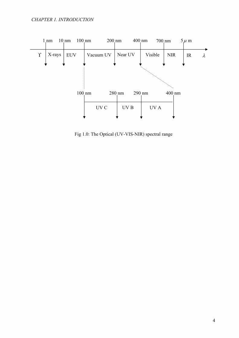
(UV). The UV radiation can be subdivided into three different groups (Fig 1.0) based on the

wavelength of the radiation (100-400 nm); these are referred to as vacuum UV (100-200 nm),

UV-C (200-280 nm), UV-B (280-320 nm), and UV-A (320-400 nm). The oxygen molecules in

the upper atmosphere and stratospheric ozone layer have large absorption cross-sections for

solar ultraviolet radiation, depending on wavelength. The absorption by the stratospheric ozone

is more effective for the shorter wavelengths and tends to reach its peak at 250 nm and drops

rapidly with an increase in wavelength to even beyond 350 nm. Thus, the biologically harmful

radiation below 200 nm (vacuum UV) is completely absorbed by oxygen molecule (O2) and

residual Nitrogen (N2) while the ozone layer completely shields the radiation in the range (200-

300 nm) with only a fraction of the UV-B and UV-A wavelength bands reaching the earth

surface. The depletion of the protective ozone layer by certain atmospheric pollutants

(Chlorofluorocarbons, halons and nitrogen oxides) that interact photochemically with ozone

will promote the transmission of highly injurious ultraviolet radiation [El-Hinnawi and Hashmi

1982].


1Solar Backscatter Ultraviolet Spectrometer on Nimbus 7 (11/1978-1990), NOAA-9, NOAA-11, and NOAA-14 (1984-date) [Heath et al., 1975]2Total Ozone Mapping Spectrometer on Nimbus 7 (11/1978-05/1993), Meteor 3 (08/1991-11/1994), and Earth-Probe (07/1996-date) [Heath et al., 1975]

4

Fig 1.0: The Optical (UV-VIS-NIR) spectral range

400 nm290 nm280 nm100 nm

200 nm 400 nm 5 m700 nm1 nm 10 nm 100 nm

X-rays EUV Vacuum UV Near UV Visible IRNIR

UV C UV B UV A


5

Chapter 2

2.0 The atmosphere

The atmosphere is the gaseous envelope that surrounds the Earth and constitutes the transition

between its surface and the vacuum of space. The early atmosphere is different from the

atmosphere of today which had evolved in 3 stages; stage I (primordial atmosphere), evolved

from the gravitational capture of the gases in the proto-planetary nebula of the sun consisting

mainly of H2 and He. Stage II (secondary atmosphere) results from the outgassing of the planet

through volcanoes, geysers, cracks etc., consisting mainly of H2O, CO2, SO2, H2S, and CO

leading to the formation of oceans with other gases from the influx of material from meteorites

and comets, and sputtering of material of the planetary surface by cosmic rays and energetic

particles. Stage III (the present atmosphere) is enriched in O2 due to photosynthesis by plants

leading to the presence of life. Since the presence of life, human activities have affected the

composition of the atmosphere and presently, the atmosphere consists by volume of a mixture

of gases composed primarily of nitrogen (78.08 %), oxygen (20.95 %), argon (0.93 %) and

other noble gases (Ne, He, Xe) (<0.003 %), hydrogen (0.00005 %), and other gases in variable

amount such as water vapour (0-4%), carbon dioxide (0.037 %), methane (1.7 ppm1), nitrous

oxide (0.3 ppm), ozone (0.0-0.07 ppm), particles (dust etc.) (< 0.15 ppm), chlorofluorocarbons

(0.0002 ppm). It extends some 500 km above the surface of the Earth and the lower level

(troposphere) constitutes the climate system that maintains the conditions suitable for life on

the earth surface. The next atmospheric level, the stratosphere (12 to 50 km), contains the

ozone layer that protects life on the planet by filtering harmful ultraviolet radiation from the

Sun. The effect of man’s activities through the burning of fossil fuels since the industrial

revolution has altered the composition of the atmosphere, of greatest concern is the rising

concentration of the greenhouse gases such as carbon dioxide, methane, nitrous oxide, and

chloroflurocarbons in the atmosphere as they trap heat energy emitted from the earth surface

thereby increasing the global temperatures (global warming) [Hansen, 1989]. In addition, they

also lead to photochemical smog and acid rain which are threats to survival on the earth

surface.

1Parts per million

6

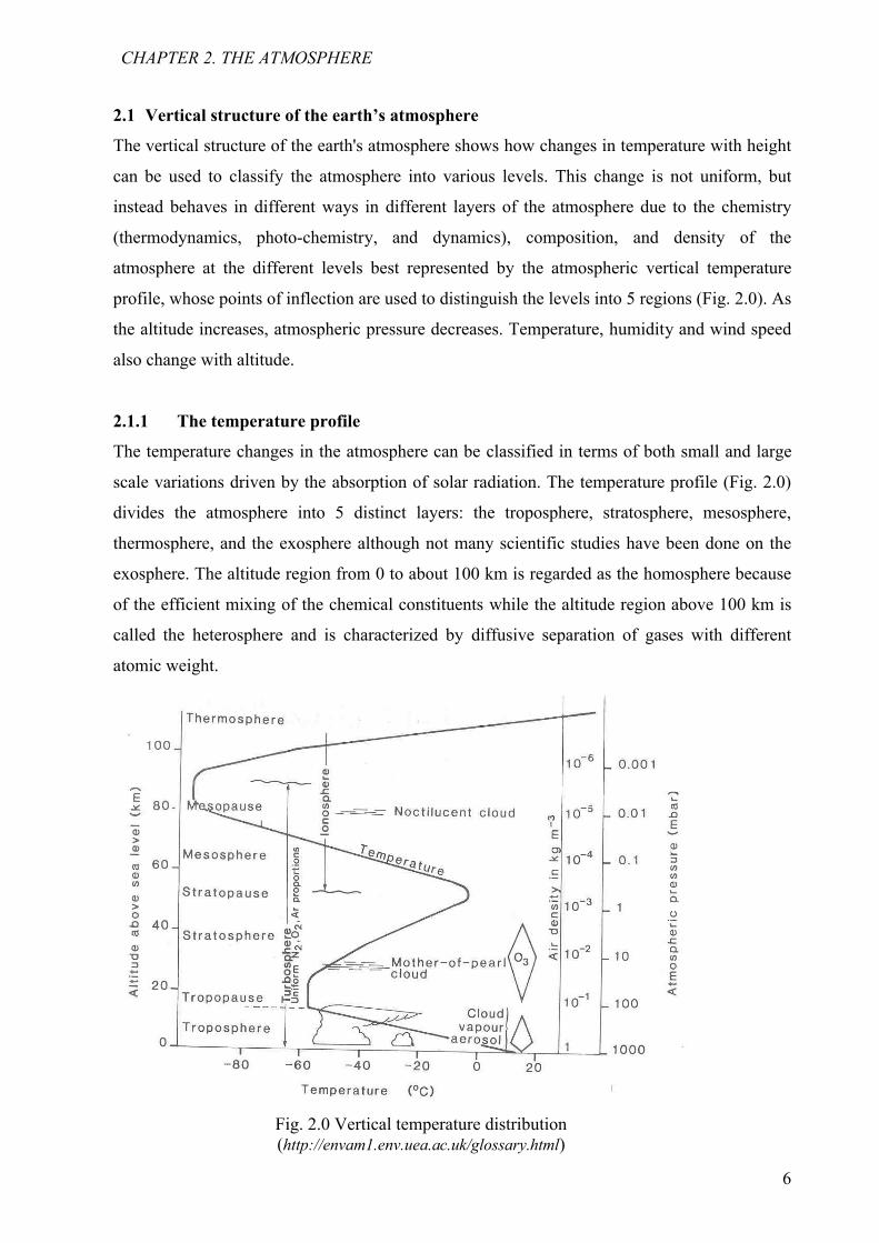
2.1 Vertical structure of the earth’s atmosphere

The vertical structure of the earth's atmosphere shows how changes in temperature with height

can be used to classify the atmosphere into various levels. This change is not uniform, but

instead behaves in different ways in different layers of the atmosphere due to the chemistry

(thermodynamics, photo-chemistry, and dynamics), composition, and density of the

atmosphere at the different levels best represented by the atmospheric vertical temperature

profile, whose points of inflection are used to distinguish the levels into 5 regions (Fig. 2.0). As

the altitude increases, atmospheric pressure decreases. Temperature, humidity and wind speed

also change with altitude.

2.1.1 The temperature profile

The temperature changes in the atmosphere can be classified in terms of both small and large

scale variations driven by the absorption of solar radiation. The temperature profile (Fig. 2.0)

divides the atmosphere into 5 distinct layers: the troposphere, stratosphere, mesosphere,

thermosphere, and the exosphere although not many scientific studies have been done on the

exosphere. The altitude region from 0 to about 100 km is regarded as the homosphere because

of the efficient mixing of the chemical constituents while the altitude region above 100 km is

called the heterosphere and is characterized by diffusive separation of gases with different

atomic weight.

Fig. 2.0 Vertical temperature distribution(http://envam1.env.uea.ac.uk/glossary.html)

CHAPTER 2. THE ATMOSPHERE

7

2.1.1.1 The troposphere

The troposphere begins at the ground and ranges in height to an average of 8-9 km at the poles

to 17 km at the equator. It is heated from the ground, which absorbs solar radiation and releases

heat back up in the infrared region. The temperature of the air in this region decreases linearly

with altitude, at a lapse rate of 5 to 7 K/km due to adiabatic cooling; as the air rises the

atmospheric pressure falls and so the air expands. For expansion to occur, work must be done

to its surroundings which lead to a decrease in temperature due to conservation of energy. This

is the most familiar region of the atmosphere, containing most of the clouds and weather

phenomena. The air in this layer is turbulent and well mixed horizontally and vertically due to

non uniform heating of the earth surface and the atmosphere. Most of the greenhouse gases

including ozone are found in this region. The ozone in this region is regarded as bad ozone as it

is a pollutant and a constituent of smog. The boundary between the troposphere and the

stratosphere is the tropopause. This is the region of the atmosphere where the lapse rate

changes from negative (in the troposphere) to positive (in the stratosphere). The tropopause is

not a “hard” boundary as vigorous thunderstorms, for example in the tropical region can

overshoot into the lower stratosphere and undergo a brief low-frequency vertical oscillation

which can set up a low-frequency atmospheric wave train capable of affecting both

atmospheric and oceanic currents in the region. The height of the tropopause varies with season

due to changes in the atmospheric circulation.

2.1.1.2 The stratosphere

The stratosphere is situated between about 10 km and 50 km altitude above the earth surface at

the lower latitudes and at about 8 km and 45 km at the poles. The temperature at the top of the

stratosphere is as high as 270 K, about the same as the ground level temperature. This layer of

the atmosphere is stratified in temperature with warmer layers higher up and cooler layers

farther down because it is heated from above due to the absorption of ultraviolet radiation by

the ozone layer. In fact it is this ozone layer that is basically responsible for the existence of the

"stratosphere." The vertical stratification, with warmer layers above and cooler layers below,

makes the stratosphere dynamically stable such that there is no regular convection and

associated turbulence in this part of the atmosphere. This layer of the atmosphere is regarded as

the region of intense interactions among radiative, dynamical, and chemical processes, in

which horizontal mixing of gaseous components proceeds much more rapidly than vertical

mixing. The stratosphere is mostly dry with the exception of the presence of winter Polar

Stratospheric Clouds (PSCs) also know as nacreous clouds. One interesting feature of the


8

stratospheric circulation is the Quasi-Biennial Oscillation (QBO) in the tropical latitudes,

which induces a secondary circulation responsible for the global stratospheric transport of

tracers such as ozone and water vapour driven by gravity waves convectively generated in the

troposphere. During winter, the contrast in temperature between orography and land and sea

breezes lead to the generation of long Rossby waves in the troposphere which eventually lead

to a sudden rise in temperature in the northern hemisphere of the stratosphere (sudden

stratospheric warming). Stratospheric warming can also be observed in the southern

hemisphere although not as frequent as those of the northern hemisphere. There are also

situations of sudden drop in temperature during winter in both hemispheres, which leads to the

formation of PSCs. In the stratosphere, ozone, though only a minor constituent with a mixing

ratio of about 6-10 ppm strongly absorbs solar UV radiation similar to the absorption of visible

light on the earth surfaces. The ozone absorption that is responsible for the temperature

increase becomes negligible at higher altitudes creating a temperature peak at about 50 km that

marks the next boundary: the stratopause, which is the boundary layer between the stratosphere

and the mesosphere.

2.1.1.3 The mesosphere

The layer just above the stratopause is the mesosphere. It is located from about 50 km to 90-

100 km altitude above the earth’s surface depending on the latitude. Within this layer,

temperature again decreases with increasing altitude due to decreasing solar heating and

increasing cooling by CO2 radiative emission. The main dynamical features in this region are

atmospheric tides, internal atmospheric gravity waves and planetary waves which are mainly

excited in the troposphere and lower stratosphere and propagate upward to the mesosphere. In

this region of the atmosphere, the gravity-wave amplitudes can become so large that the waves

become unstable and dissipate thereby creating momentum in the mesosphere which drives the

mesospheric meridional circulation. The temperatures in the upper mesosphere can fall as low

as 100 K varying according to latitude and season. Millions of meteors burn up daily in the

mesosphere as a result of collisions with the gas particles contained there; this creates enough

heat to vaporize almost all of the falling objects long before they reach the ground, thereby

resulting in a high concentration of iron and other metal atoms in this region of the atmosphere.

The minimum in temperature at the top of the mesosphere is called the mesopause, which is the

coldest place in the atmosphere; it is the mesopause that separates the mesosphere from the

thermosphere.


9

2.1.1.4 The thermosphere

This is the layer of the earth’s atmosphere that extends from about 90-100 km to 400 km above

the earth's surface. In this layer, the temperature increases with altitude due to the absorption of

highly energetic solar radiation by nitrogen and residual oxygen which are partially converted

into ions forming a layer called the ionosphere which begins from the upper mesosphere. The

temperature in this region is as high as 2500 K during the day, although may not be felt as a

thermometer in this region will read 0 K due to the large mean free path between the few atoms

of gas which are supposed to transfer heat since it is close to vacuum. Atmospheric tides

dominate the lower part of the thermosphere but dissipate towards the top as the concentration

of the molecules is not high enough to support the motion needed for fluid flow. Aurorae are

also formed in this layer of the atmosphere. The thermopause separates the thermosphere from

the exosphere.

2.1.1.5 The exosphere

This is the outermost layer of the atmosphere ranging from about 500 km to 1000 km and may

sometimes extend to about 10000 km above the earth surface due to the energy input of

location, time of day, solar flux, season, and other atmospheric properties. The gases in this

layer are the light gases such as hydrogen, helium, and atomic oxygen near the critical level

(exobase) which may sometimes escape to space. It is this region of the atmosphere that many

satellite orbit the earth.

2.1.2 The pressure and density profile

Pressure (P) and density (ρ) decrease nearly exponentially with height, according to the

relation:

where P(z) is the pressure at height z, Po is the pressure at some reference level, which is

usually taken as sea level (z = 0), and H (e-folding depth) referred to as the scale height is

given by:

where M is the molecular mass, g is the gravitational acceleration, k is Boltzmann's constant,

and T is the absolute temperature. The drop in pressure by a factor e is the direct result of

hydrostatic balance leading to the pressure gradient equation:

/( ) z HoP z P e (2.0)

(2.1)

p g (2.2)

kTH

Mg


10

where p is the pressure, ρ is mass density, and g is the gravitational acceleration. The solution

of the pressure gradient equation leads to a scale height ranging from 3 to 8 km throughout the

lowest 100 km. This means that 90 % of the atmospheric mass is in the troposphere and only

10 % in the stratosphere. Therefore, dividing equation (2.0) by Po and taking the natural

logarithm yields:

Equation (2.3) is useful for the estimation of the height of various pressure levels in the Earth’s

atmosphere, because the pressure at a given height in the atmosphere is a measure of the mass

that lies above the level and is sometimes used as vertical coordinate in lieu to height.

Atmospheric pressure varies smoothly with height and there are no signs of any fine structure

in the vertical pressure profile corresponding to those in the associated temperature profile and

the horizontal pressure variations are very much smaller and smoothly distributed. As stated

above, density also decreases with height in the same manner as pressure and the vertical

variations in pressure and density are much larger than the corresponding horizontal and time

variations. Fig. 2.1 shows a semi log plot of the vertical profile of pressure, density and mean

free path for a standard atmosphere from 0 to about 160 km above the earth surface.

(2.3)

Fig. 2.1: Vertical profile of pressure, density and mean free path for a standard atmosphere

(see Atmos. Phys. by John Michael Wallace, Peter Victor Hobb)

lno

p z

p H


11

Chapter 3

3.0 Ozone chemistry

3.1 Stratospheric ozone

Stratospheric Ozone, which is about 90 % of the ozone (O3) in the earth atmosphere, is found

in the region from about 10-50 km above the earth’s surface where it forms a layer about 20

km thick (Fig. 3.1). The amount of ozone in this region of the atmosphere varies, depending

mainly on latitude and season, where its presence causes stratospheric temperature inversion

and a resulting temperature peak at the stratopause. Fabry and Buisson [1921], who conducted

the first detailed measurements of the atmospheric column of ozone, stated that ozone was

responsible for the observed strong cut-off in solar UV spectra at about 300 nm towards shorter

wavelengths. They also suggested that ozone is formed by solar UV radiation and that the

ozone layer is situated at an altitude of about 50 km, which was equally confirmed by other

scientists to be about 48-53 km [Cabannes and Dufay, 1925; Lambert et al., 1926]. In addition

to its radiation properties, ozone reacts with many other trace species, some of which are

anthropogenic in origin. It plays a vital role in the earth atmosphere by absorbing the

biologically harmful UV radiation from the sun. Without ozone, the surface of the Earth would

be bathed in UV radiation, which is harmful to the eyes and skin and could also result in

damage to crops and marine phytoplankton1 as well as being able to break DNA2 molecular

bonds. It has been observed that recent anthropogenic chemical additions to the atmosphere

can destroy ozone [Cicerone, 1974; Molina and Rowland, 1974], also research has shown that

stratospheric ozone concentrations have declined over the past three or four decades [Wayne,

2000]. However, there have been some recent speculations that the ozone loss rate is

decreasing due to conformity with the Montreal Protocol3 adopted on September 16, 1987

[Weatherhead et al., 2000; Newchurch et al., 2003].

3.2 Ozone absorption theory

As mentioned earlier, ultraviolet radiation with a wavelength of less than 180 nm does not

reach the stratosphere; from 180-240 nm it is absorbed primarily by O2 to form O3 and does not

reach the lower stratosphere. From 240-290 nm it is absorbed by O3 and does not reach the

earth’s surface; from 280-320 nm (UV-B) the radiation is partially absorbed by ozone and the

portion that reaches the earth’s surface is largely responsible for sunburn, skin cancer and other

biological effects. From 320-400 nm (UV-A) the radiation is mostly transmitted to the ground

and may be important in the formation of photo-chemical smog. The absorption spectrum of

ozone in the UV to NIR1 spectral regions is divided into four different absorption bands: The

1near infrared

12

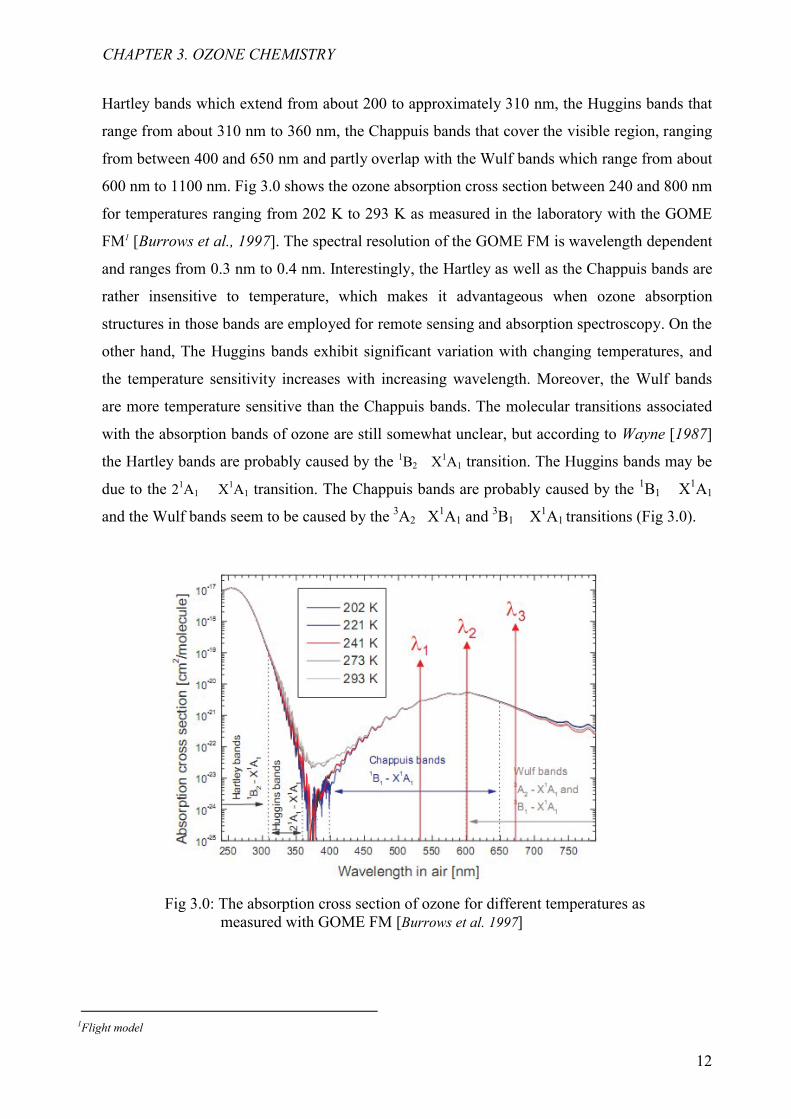
Hartley bands which extend from about 200 to approximately 310 nm, the Huggins bands that

range from about 310 nm to 360 nm, the Chappuis bands that cover the visible region, ranging

from between 400 and 650 nm and partly overlap with the Wulf bands which range from about

600 nm to 1100 nm. Fig 3.0 shows the ozone absorption cross section between 240 and 800 nm

for temperatures ranging from 202 K to 293 K as measured in the laboratory with the GOME

FM1 [Burrows et al., 1997]. The spectral resolution of the GOME FM is wavelength dependent

and ranges from 0.3 nm to 0.4 nm. Interestingly, the Hartley as well as the Chappuis bands are

rather insensitive to temperature, which makes it advantageous when ozone absorption

structures in those bands are employed for remote sensing and absorption spectroscopy. On the

other hand, The Huggins bands exhibit significant variation with changing temperatures, and

the temperature sensitivity increases with increasing wavelength. Moreover, the Wulf bands

are more temperature sensitive than the Chappuis bands. The molecular transitions associated

with the absorption bands of ozone are still somewhat unclear, but according to Wayne [1987]

the Hartley bands are probably caused by the 1B2 X1A1 transition. The Huggins bands may be

due to the 21A1 X1A1 transition. The Chappuis bands are probably caused by the 1B1 X1A1

and the Wulf bands seem to be caused by the 3A2 X1A1 and 3B1 X

1A1 transitions (Fig 3.0).

Fig 3.0: The absorption cross section of ozone for different temperatures as measured with GOME FM [Burrows et al. 1997]

1Flight model

CHAPTER 3. OZONE CHEMISTRY

13

3.3 Ozone profile

Ozone profile1 (Fig 3.1) measurements taken by balloon borne instruments known as

ozonesondes, laser2 instruments called lidar3, and profiling satellite instruments are usually

reported in mixing ratio, number density, or partial pressure. Mixing ratio in ppmv4

corresponds to the fractional concentration of ozone as the number of ozone molecules per

million air molecules. Number density refers to the absolute concentration as the number of

ozone molecules per cubic centimeter. Partial pressure refers to the fraction of the atmospheric

pressure at a given altitude for which ozone is responsible. Ozone profiles measured in each of

these units appear somewhat different with only a close similarity between number density and

partial pressure profiles because the partial pressure of ozone can be expressed as a function of

the number density according to the relation

Where N is the number density, k is the Boltzmann’s constant and T is the temperature in

Kelvin.

Fig 3.1 shows the ozone profile in number density, partial pressure and mixing ratio, measured

by SAGE II at 40oS on September 11, 1994. From the three profiles, it can be observed that the

ozone layer peak occurs at altitudes between 20 and 40 km. In the case of the mixing ratio

profile, the peak is significantly higher in altitude than for the number density and partial

P NkT (3.0)

Number density(Molecules/cm3)(x10-12)

Partial pressure (nb) Mixing ratio (ppmv)

Fig. 3.1 The ozone profile(see http://www.ccpo.odu.edu/SEES/ozone/)


1ozone amount versus altitude2light amplification by stimulated emission of radiation3light detection and ranging; 4Parts per million by volume

14

pressure profiles. Also, there is a small peak between 8 and 10 km in the number density and

partial pressure profiles and not well observable in the mixing ratios profile for such a linear

scale because the mixing ratio only accounts for the fractional composition of the air molecules

at this region of the atmosphere.

3.4 Ozone chemistry and the Chapman cycle

The first theoretical explanation of the ozone layer was proposed by Chapman (1930), who

developed a steady-state photochemical model based on oxygen-only reactions. The

combination of Chapman’s reaction scheme and the insights from the past 78 years lead to the

following reactions

Where M (in 3.1b and 3.1f) is another molecule (typically N2 or O2) which carries away the

extra energy of the three body reaction.

The reactions in (3.1) can be classified into three different groups namely:

1. Those that produce odd-oxygen (the combination of [O] and [O3]), e.g., reaction (3.1a)

2. Those that balance the ratio of atomic oxygen (O) and O3 concentrations, e.g., reactions

(3.1b) and (3.1c)

3. Those that destroy odd oxygen, e.g., reactions (3.1d), (3.1e), and (3.1f).

Reactions (3.1a), (3.1b), and (3.1c) provide the mechanism for converting UV-light into heat

with reactions (3.1b) and (3.1c) being very efficient at the inter-conversion of O and O3, even

at the top of the atmosphere where the pressure is low, thereby leading to the concept of odd

oxygen which is produced only in reaction (3.1a) and lost in reactions (3.1d), (3.1e), and (3.1f).

However, due to the low concentration of O in the stratosphere, reaction (3.1f) is too slow in

comparison with reactions (3.1d) and (3.1e) and so can be neglected. At higher altitude,

reaction (3.1b) slows down while reaction (3.1c) becomes faster, thus atomic oxygen is

favoured at higher altitudes while O3 is favoured at lower altitudes. At altitudes below 60 km,

ozone is the dominant form of odd oxygen so it forms about 99 % of odd oxygen in the

stratosphere and its rate of production can be equated with the rate of the O atom formation

which is twice the rate of O2 photolysis (3.1a). The dissociation of ozone leading to the

1 32

2 3

1 13 2

3 2

3 3 2 2 2

2

( ) ( ) [ 242 ]

( ) ( ) [ 320 ]

2

g

O hv O D O P nm

O O M O M

O hv O D O nm

O O O

O O O O O

O O M O M

(3.1a)

(3.1b)

(3.1c)

(3.1d)

(3.1e)

(3.1f)


15

production of O and O2 can also occur a little above 320 nm and by the absorption in the

Chappuis band. According to the steady-state model, since most of the odd oxygen is in the

form of ozone, it can be stated that stratospheric ozone concentrations are proportional to the

square root of the rate of the photolysis of oxygen (3.1d) [Wayne, 1987]. Though the odd

oxygen reactions provide a basic foundation for understanding the sources and sinks for odd

oxygen, they do not give a proper detail of the processes involved. The production mechanism

for O3 can be described by the combination of reactions (3.1a) and (3.1b)

After sunset, reactions (3.1a) and (3.1c) stop while reaction (3.1b) and (3.1d) remain, thus

allowing the concentration of the atomic oxygen to drop and ozone is no longer destroyed in

(3.1d). Since the ratio of the concentration of O to that of O3 is governed by the rapid

photochemical reactions which interconvert O and O3, at steady state, the rate of creation of

ozone from three body collisions will be equal to the rate of photodissociation of ozone by

sunlight. This can be expressed as:

where the brackets [] around a chemical symbol indicate the concentration of the chemical in

molecules/cm3; 2( , )O OK is the reaction rate coefficient for the reaction of O with O2 in cm6

molecule-2 sec-1, and3Oj is the photodissociation coefficient for O3 in molecule-1 sec-1. As the

reaction rate of (3.1b) decreases with increasing altitude, the ratio of the concentration of ozone

to that of atomic oxygen [O3]/[O] decreases with increasing altitude as both [O2] and [M] fall

off exponentially. At 50 km, the daytime ratio of [O]/[O3] is a little less than 0.1. Thus, ozone

at 50 km will increase by about 10 % at night and then decrease again as sunlight returns.

Also, the measured rate of reaction of (3.1d) is much smaller than that required by the oxygen

only model.

3.5 Incompleteness of the Chapman cycle

Although the Chapman cycle was an important step towards a better understanding of the

chemistry of stratospheric ozone, it was incomplete as it could not address some important

issues such as:

2

2 3

2 3

2

2 2 2 2 2

3 2

O hv O

O O M O M

O hv O

(3.2)

(3.3)

(3.4)


2 3( , ) 2 3[ ][ ][ ] [ ]O O OK O O M J O

3 23 ( ) ( , ) 2[ ] / [ ] / [ ][ ]O O OO O J K O M

16

1. The ozone column being very small at the tropics (where the solar zenith angle (SZAs)

is small) and maximum at the temperate and high latitude.

2. The predictions of ozone densities are a factor of 2 higher than observed densities in the

tropics

3. The predictions of the Chapman model being too low at the polar latitudes.

It has been found that these inconsistencies disappear if additional odd oxygen loss

mechanisms, i.e. the ozone catalytic destruction cycles involving hydrogen, halogen and

nitrogen compounds, as well as the Brewer-Dobson1 circulation are considered. The work of

Bates and Nicolet [1950] on the odd hydrogen reaction (HOx i.e H, OH, HO2), showed that the

rate of reaction of (3.1e) can be increased by the presence of a catalyst as shown below:

It was also observed that the rate of reaction of (3.1d) could also be increased catalytically by

e.g.:3 2

2

3 2 2

Cl O ClO O

ClO O Cl O

O O O O

(3.6)

(3.5)

(3.7)

3 2

2

3 2 2

Br O BrO O

BrO O Br O

O O O O

3 2

2

3 2 2

H O OH O

OH O H O

O O O O

3 2 2

2 2

3 2 2

OH O HO O

HO O OH O

O O O O

(3.8)


(3.9)

3 2 2

2 3 2 2

3 3 2 2 2

OH O HO O

HO O OH O O

O O O O O

1slow stratospheric equator-to-pole motion

17

Crutzen [1970] and Johnston [1971] investigated the impact of NOx (NO and NO2) on ozone

which accounts for about 70 % of ozone loss at 30 km altitude (3.10).

As shown in above (3.6-3.10), the net effect of the reactions is the formation of 2 oxygen

molecules from an ozone molecule and an oxygen atom while the NO-NO2 and Cl-ClO are

unaffected. At about 40 km altitude, these catalytic processes can destroy nearly 1000 ozone

molecules before the catalyst (NO-NO2 and Cl-ClO) becomes inactive and forms reservoir

species such as Hydrochloric acid (HCl) or Chlorine nitrate (ClONO2) where they last for a

few days before they are photolyzed. During photolysis the Cl atom is released which then

starts the ozone destruction process once again; eventually the Cl atom is carried out of the

stratosphere. Therefore the amount of ozone in the stratosphere is due to a balance between the

solar production and the loss by a number of these catalytic reactions. If it were possible to

increase the solar ultraviolet output at wavelengths below 240 nm, ozone levels would rise.

The loss of ozone in the natural form results from normal levels of gases such as methane,

nitrous oxide, methyl bromide, and methyl chloride, so if there is an increase in these natural

levels of chlorine, nitrogen, bromine or hydrogen in the stratosphere, or if new compounds are

added to the stratosphere, the loss of ozone will increase, and the level of ozone will decrease,

until a new equilibrium between production and loss is achieved.

3.6 Chapman layers

Due to the variation in optical density of the atmosphere, species such as ozone whose

concentration depend on photochemical production, form layer-like structures called Chapman

layers having a profile defined by the Chapman function. The shape of the Chapman layer can

be explained by a simple model in which incident light travels downward from the top of the

atmosphere. Although the solar intensity is higher at the top of the atmosphere, little amounts

of atomic oxygen are produced due to the low concentration of O2. As the light travels through

the atmosphere, it interacts with the atmospheric medium and decreases in intensity such that at

lower altitude the solar intensity has decreased to an extent that despite the abundance of O2

not enough oxygen atoms can be produced. But somewhere in between there is a compromise

that maximizes the production of O atoms due to photolysis and this is the region where the

ozone layer is formed. Wayne [2000] described a simple derivation of the Chapman function

starting with:

3 2 2

2 2

3 2 2

NO O NO O

NO O NO O

O O O O

(3.10)


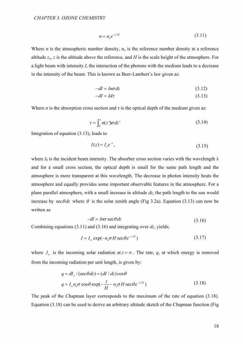
18

Where n is the atmospheric number density, no is the reference number density at a reference

altitude zo, z is the altitude above the reference, and H is the scale height of the atmosphere. For

a light beam with intensity I, the interaction of the photons with the medium leads to a decrease

in the intensity of the beam. This is known as Beer-Lambert’s law given as:

Where σ is the absorption cross section and τ is the optical depth of the medium given as:

Integration of equation (3.13), leads to

where I0 is the incident beam intensity. The absorber cross section varies with the wavelength λ

and for a small cross section, the optical depth is small for the same path length and the

atmosphere is more transparent at this wavelength. The decrease in photon intensity heats the

atmosphere and equally provides some important observable features in the atmosphere. For a

plane parallel atmosphere, with a small increase in altitude dz, the path length to the sun would

increase by sec dz where is the solar zenith angle (Fig 3.2a). Equation (3.13) can now be

written as

Combining equations (3.11) and (3.16) and integrating over dz, yields;

where I is the incoming solar radiation at z . The rate, q, at which energy is removed

from the incoming radiation per unit length, is given by:

The peak of the Chapman layer corresponds to the maximum of the rate of equation (3.18).

Equation (3.18) can be used to derive an arbitrary altitude sketch of the Chapman function (Fig

/z Hon n e

dI In dz

dI Id

0( ') '

zn z dz

( ) ,oI z I e

(3.11)

(3.12)

(3.13)

(3.14)

(3.15)

- secdI In dz (3.16)

/exp( sec )z HoI I n H e

/

/ (sec ) ( / ) cos

cos exp( sec )

z

z Ho o

q dI dz dI dz

zq I n n H e

H

(3.17)

(3.18)


19

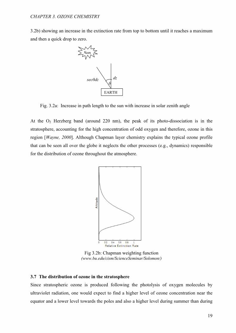
3.2b) showing an increase in the extinction rate from top to bottom until it reaches a maximum

and then a quick drop to zero.

At the O2 Herzberg band (around 220 nm), the peak of its photo-dissociation is in the

stratosphere, accounting for the high concentration of odd oxygen and therefore, ozone in this

region [Wayne, 2000]. Although Chapman layer chemistry explains the typical ozone profile

that can be seen all over the globe it neglects the other processes (e.g., dynamics) responsible

for the distribution of ozone throughout the atmosphere.

3.7 The distribution of ozone in the stratosphere

Since stratospheric ozone is produced following the photolysis of oxygen molecules by

ultraviolet radiation, one would expect to find a higher level of ozone concentration near the

equator and a lower level towards the poles and also a higher level during summer than during

Fig. 3.2a: Increase in path length to the sun with increase in solar zenith angle

Fig 3.2b: Chapman weighting function (www.bu.edu/cism/ScienceSeminar/Solomon/)


Sun

θdzsecθdz

EARTH

20

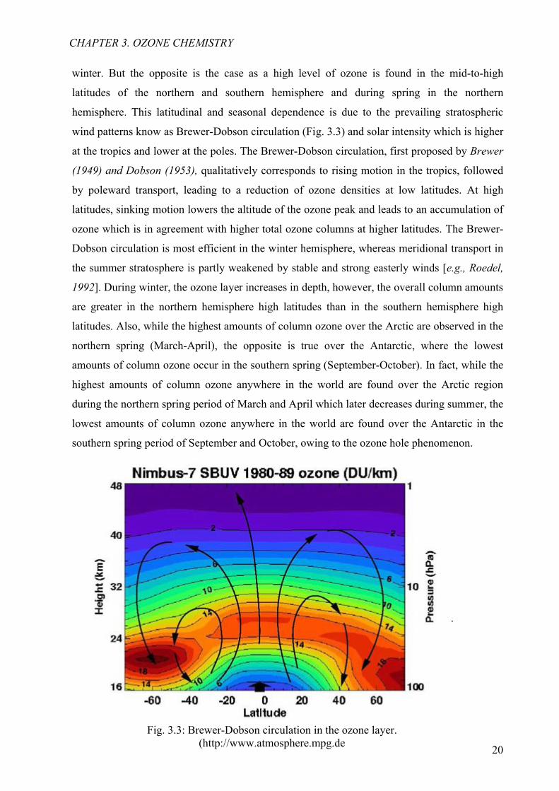
winter. But the opposite is the case as a high level of ozone is found in the mid-to-high

latitudes of the northern and southern hemisphere and during spring in the northern

hemisphere. This latitudinal and seasonal dependence is due to the prevailing stratospheric

wind patterns know as Brewer-Dobson circulation (Fig. 3.3) and solar intensity which is higher

at the tropics and lower at the poles. The Brewer-Dobson circulation, first proposed by Brewer

(1949) and Dobson (1953), qualitatively corresponds to rising motion in the tropics, followed

by poleward transport, leading to a reduction of ozone densities at low latitudes. At high

latitudes, sinking motion lowers the altitude of the ozone peak and leads to an accumulation of

ozone which is in agreement with higher total ozone columns at higher latitudes. The Brewer-

Dobson circulation is most efficient in the winter hemisphere, whereas meridional transport in

the summer stratosphere is partly weakened by stable and strong easterly winds [e.g., Roedel,

1992]. During winter, the ozone layer increases in depth, however, the overall column amounts

are greater in the northern hemisphere high latitudes than in the southern hemisphere high

latitudes. Also, while the highest amounts of column ozone over the Arctic are observed in the

northern spring (March-April), the opposite is true over the Antarctic, where the lowest

amounts of column ozone occur in the southern spring (September-October). In fact, while the

highest amounts of column ozone anywhere in the world are found over the Arctic region

during the northern spring period of March and April which later decreases during summer, the

lowest amounts of column ozone anywhere in the world are found over the Antarctic in the

southern spring period of September and October, owing to the ozone hole phenomenon.

.


Fig. 3.3: Brewer-Dobson circulation in the ozone layer.(http://www.atmosphere.mpg.de

21

3.8 History of the Chlorofluorocarbons (CFCs)

The Chlorofluorocarbons (CFCs), also called Freons, are a group of chemical compounds

comprising carbon, fluorine, and chlorine. CFCs were invented in the early 1930s as

propellants for aerosols, refrigeration coolants, and electronic circuit board cleaners. After it

was shown by Crutzen [1970] that nitric oxide (NO) could catalyze the destruction of ozone,

chemists Frank Sherwood Rowland and Mario Molina in 1973 began studying the impacts of

CFCs in the earth's atmosphere. In 1974, Stolarski and Cicerone [1974] first demonstrated that

chlorine can also catalyze the destruction of ozone. In the same year, Rowland and Molina

found that CFC molecules were stable enough to remain in the atmosphere for about 50-200

years before they reached the middle of the stratosphere where they are finally broken down by

ultraviolet radiation (3.19) thereby releasing chlorine atoms [Rowland et al. 1989, 1991]. They

then proposed that these chlorine atoms might be expected to cause the breakdown of large

amounts of ozone in the stratosphere. The Rowland-Molina hypothesis suffered a lot of set-

backs mainly from the criticisms by the representatives of the aerosols and halocarbon

industries but the scientific community was shocked when British Antarctic Survey scientists

Farman, Gardiner and Shanklin [1985] published a journal paper showing a sharp decline in

polar ozone over Antarctica in southern hemisphere spring. This led to some nations coming

together to establish a framework for negotiating international regulations on ozone-depleting

substances (ODS) and consequently Crutzen, Molina and Rowland were awarded a Nobel

Prize for Chemistry in 1995 for their findings.

2O3 3O2

3.9 The Montreal protocol and its amendments

The Montreal protocol, an international treaty designed to protect the ozone layer by phasing

out the production of ozone depleting substances such as the halogen compounds

(chlorofluorocarbon (CFC) commonly called freons, and bromofluorocarbon compounds

known as halons) and a number of chemical compounds (carbon tetrachloride and

trichloroethane etc.), was opened by 24 nations for signature on September 16, 1987 and

adopted on January 1, 1989 followed by a first meeting in Helsinki, May 1989 and has since

.3 2

. .3 2

.3 2

2 2

.2 2 2

2

2

CFCl hv CFCl Cl

Cl O ClO O

ClO O Cl O

ClO ClO M Cl O M

Cl O hv Cl O

(3.19)


22

then undergone some amendments: in 1990 (London), 1991 (Nairobi), 1992 (Copenhagen),

1993 (Bangkok), 1995 (Vienna), 1997 (Montreal) and 1999 (Beijing) as shown in (Fig. 3.4),

with over 190 countries currently joining the campaign while countries like Andorra, Iraq, San

Marino, Timor-Leste and Vatican City were still yet to join as of September 2007. These

amendments have resulted in a more rapid decline of ozone depleting substances [Showstack,

2003, Anderson, et al., 2000]. It is believed that if the international agreement is adhered to, the

ozone layer is expected to recover by 2050. The countries ratifying the Montreal protocol

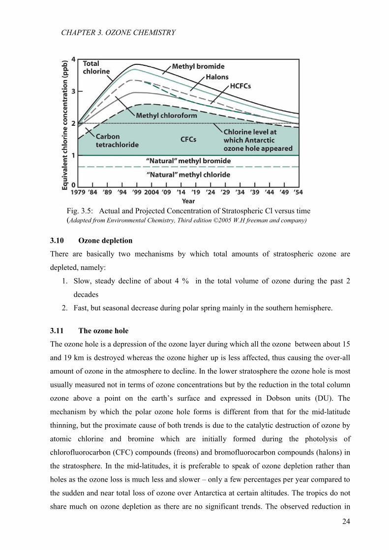
committed themselves to reducing the production and consumption of 5 CFC compounds

(CFCl3 (CFC-11), CF2Cl2 (CFC-12), C2F3Cl3 (CFC-113), C2F4Cl2 (CFC-114), and C2F5Cl

(CFC-115)) and 3 halons (halon 1211, 1301, and 2402) (Fig. 3.5). According to the protocol,

developed countries were required to phase out the production and consumption of the 5

regulated CFCs by January 1, 1996 and the production and consumption of the regulated

halons by January 1, 1994 while for developing countries with a per capita consumption of the

regulated substances below a certain threshold (0.3 kg per year) were given the deadline of

about 2010. There are a few exceptions of the substances (e.g. the metered dose inhalers

commonly used to treat asthma and other respiratory problems or halon fire suppression

systems used in submarines and aircraft) that are still in essential use because no acceptable

substitutes have been found. Based on this, several reports have been published by various

institutions, governmental and non-governmental organizations to present alternatives to the

ozone depleting substances, since these substances are still useful in various technical sectors

such as agriculture, refrigerating, laboratory measurements and energy production. Recent

research has shown that since the Montreal protocol came into effect, the atmospheric

abundances of several regulated species have decreased in the lower atmosphere since mid of

the 1990s (e.g. CFC-11) [Egorova, 2001]. It is also noted that the abundances of species with

longer atmospheric lifetimes (e.g. CFC-12) do not increase anymore and are expected to

decrease over the next few years. Although halon concentrations have been found to be

increasing as halons presently stored in fire extinguishers are released but they are expected to

decline by 2020. Also the concentration of Hydrochlorofluorocarbons (HCFCs) has increased

drastically because they were used to replace CFCs in solvents or refrigerating agents. The

HCFCs and Hydrofluorocarbons (HFCs) have been found to have a larger greenhouse gas

potential (on a per molecule basis), but the total effect is still significantly smaller than that of

the anthropogenic CO2. At the moment, the Montreal protocol has placed a restriction on

HCFCs by 2030 but non on HFCs. The substitution of HFCs for CFCs is currently not showing

any significant increase in global warming but there is the likelihood that over time, a steady

CHAPTER 3. OZONE CHEMISTRYCHAPTER 3. OZONE CHEMISTRYCHAPTER 3. OZONE CHEMISTRY

23

increase in their use could lead to enhanced global warming, also worrisome is the case of

smuggling of CFCs from undeveloped to developed countries. Interestingly satellite

measurements at the end of 1990s showed that the stratospheric chlorine load does not increase

anymore, but decreases slowly [WMO 2007]. Although, this has not yet resulted in a significant

reduction in the size of the ozone hole [Newman et al. 2006]. However, in the altitude range of

40 km, where the first papers [Crutzen 1974, Cicerone et al., 1974] already predicted the

greatest effects of chlorine on ozone destruction, there are possible signs of the beginning of

ozone recovery [Newchurch et al., 2003, Steinbrecht et al., 2009, Zanis et al., 2006, Jones et

al., 2009]. In fact, the Montreal protocol has often been called the most successful international

environment agreement to date.

Fig. 3.4: The effects of the Montreal protocol amendments and their phase-out schedules (see http://www.epa.gov/ozone/intpol/history.html)


24

3.10 Ozone depletion

There are basically two mechanisms by which total amounts of stratospheric ozone are

depleted, namely:

1. Slow, steady decline of about 4 % in the total volume of ozone during the past 2

decades

2. Fast, but seasonal decrease during polar spring mainly in the southern hemisphere.

3.11 The ozone hole

The ozone hole is a depression of the ozone layer during which all the ozone between about 15

and 19 km is destroyed whereas the ozone higher up is less affected, thus causing the over-all

amount of ozone in the atmosphere to decline. In the lower stratosphere the ozone hole is most

usually measured not in terms of ozone concentrations but by the reduction in the total column

ozone above a point on the earth’s surface and expressed in Dobson units (DU). The

mechanism by which the polar ozone hole forms is different from that for the mid-latitude

thinning, but the proximate cause of both trends is due to the catalytic destruction of ozone by

atomic chlorine and bromine which are initially formed during the photolysis of

chlorofluorocarbon (CFC) compounds (freons) and bromofluorocarbon compounds (halons) in

the stratosphere. In the mid-latitudes, it is preferable to speak of ozone depletion rather than

holes as the ozone loss is much less and slower – only a few percentages per year compared to

the sudden and near total loss of ozone over Antarctica at certain altitudes. The tropics do not

share much on ozone depletion as there are no significant trends. The observed reduction in

Fig. 3.5: Actual and Projected Concentration of Stratospheric Cl versus time (Adapted from Environmental Chemistry, Third edition ©2005 W.H freeman and company)


25

stratospheric temperatures can also be explained by the ozone depletion. Since the stratosphere

is mainly warmed by the absorption of UV radiation by ozone, a reduction in ozone amount

would result in the cooling of the stratosphere, although some stratospheric cooling is predicted

from increase in greenhouse gases such as CO2, ozone induced cooling is found to be probably

dominant.

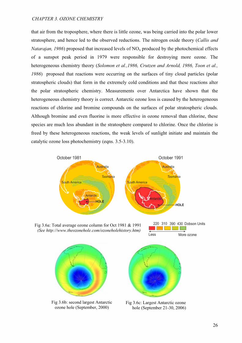
The Antarctic ozone hole discovered in the early 80s by Farman et al. [1985] and later

confirmed by other scientists [see Hofmann et al., 1987, 1997; Iwasaka and Kondoh, 1987], is

the region of the Antarctic stratosphere where the ozone level was noticed to have dropped to

about 33 % of their pre-1975 values during southern spring. The Antarctic ozone hole (Fig.

3.6) occurs during the Antarctic spring (September to early December) after the formation of

an atmospheric container called the polar vortex by strong westerly winds that circulate around

the continent. Observations taken in the Antarctic region from aircraft, the ground, and

satellites have demonstrated that the ozone hole results from the increased amounts of chlorine

and bromine in the stratosphere, combined with the peculiar meteorology of the southern

hemisphere, cold temperature during polar winter, ice cloud formation and polar sunrise during

spring that produces the energy necessary for the catalytic reactions. Ground based

measurements of ozone started first in 1956, at Halley Bay in Antarctica while satellite

measurements of ozone started in the early 70s, with the first comprehensive worldwide

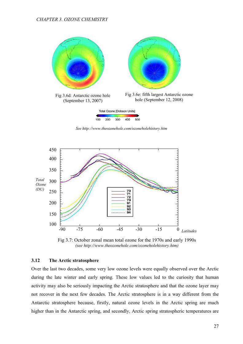
measurements in 1978 with the Nimbus-7 satellite. In the early 1990s, when the Total Ozone

Mapping Spectrometer (TOMS) was used to measure the ozone column amount, they showed a

noticeable decrease in column ozone (less than 220 DU) in the Antarctic spring and early

summer when the obtained results were compared to that obtained in the early 1970s (about

300-350 DU) (Fig 3.7). It was observed that the hole was first larger than the Antarctic

continent in 1987 and became more alarming on September 03, 2000 when the hole was

noticed by groups of British Antarctic survey and NASA1 to have covered 28.4x106 km2 and

30.3x106 km2 respectively. An increase in the ozone depletion area was later noticed on

September 5, 2006 and was recorded to cover about 29.5 x106 km2 by NASA and 28.0x106 km2

by ESA2. Currently, measurements by NASA on September 12, 2008, have also shown a

decrease in the ozone amount when compared to that of September 15, 2007 and was classified

as the fifth largest Antarctic ozone hole covering about 27x106 km2. Some theories which were

proposed to account for the existence of the "hole" include the dynamical theory, the nitrogen

oxide theory, and the heterogeneous chemistry theory. The dynamical theory (Tung et al.,

1986) proposed that the atmospheric circulation over Antarctica had changed in such a way


1National Aeronautics and Space Administration established on July 29, 19582European Space Agency established in 1975

26

that air from the troposphere, where there is little ozone, was being carried into the polar lower

stratosphere, and hence led to the observed reductions. The nitrogen oxide theory (Callis and

Natarajan, 1986) proposed that increased levels of NOx produced by the photochemical effects

of a sunspot peak period in 1979 were responsible for destroying more ozone. The

heterogeneous chemistry theory (Solomon et al.,1986, Crutzen and Arnold, 1986, Toon et al.,

1986) proposed that reactions were occurring on the surfaces of tiny cloud particles (polar

stratospheric clouds) that form in the extremely cold conditions and that these reactions alter

the polar stratospheric chemistry. Measurements over Antarctica have shown that the

heterogeneous chemistry theory is correct. Antarctic ozone loss is caused by the heterogeneous

reactions of chlorine and bromine compounds on the surfaces of polar stratospheric clouds.

Although bromine and even fluorine is more effective in ozone removal than chlorine, these

species are much less abundant in the stratosphere compared to chlorine. Once the chlorine is

freed by these heterogeneous reactions, the weak levels of sunlight initiate and maintain the

catalytic ozone loss photochemistry (eqns. 3.5-3.10).

Fig 3.6a: Total average ozone column for Oct 1981 & 1991(See http://www.theozonehole.com/ozoneholehistory.htm)

Fig 3.6c: Largest Antarctic ozone hole (September 21-30, 2006)

Fig 3.6b: second largest Antarctic ozone hole (September, 2000)


27

3.12 The Arctic stratosphere

Over the last two decades, some very low ozone levels were equally observed over the Arctic

during the late winter and early spring. These low values led to the curiosity that human

activity may also be seriously impacting the Arctic stratosphere and that the ozone layer may

not recover in the next few decades. The Arctic stratosphere is in a way different from the

Antarctic stratosphere because, firstly, natural ozone levels in the Arctic spring are much

higher than in the Antarctic spring, and secondly, Arctic spring stratospheric temperatures are

Fig 3.7: October zonal mean total ozone for the 1970s and early 1990s(see http://www.theozonehole.com/ozoneholehistory.htm)

450

400

350

300

250

200

150

100Latitudes-90 -75 -60 -45 -30 -15 0

Total Ozone (DU)

Fig 3.6e: fifth largest Antarctic ozone hole (September 12, 2008)

Fig 3.6d: Antarctic ozone hole (September 13, 2007)

See http://www.theozonehole.com/ozoneholehistory.htm


28

higher than those in the Antarctic stratosphere. As a result of the higher Arctic stratospheric

temperatures, polar stratospheric clouds are much less common in the Arctic and its polar vortex

is warmer and much more variable than the Antarctic vortex leading to a stronger inter-annual

variability in both chemical loss of ozone and in dynamical supply of ozone-rich air to high latitudes.

Therefore compared to the Antarctic, Arctic ozone trends are much more variable and higher due to the

structure of the Northern Hemisphere (Fig. 3.8). However, the Arctic winter time shares some

resemblance with that of the Antarctic, in that it also exhibits a cold polar vortex that separates

the air enclosed in it form the mid-latitude air, and there is also the transport of air from the

upper stratosphere and partly from the mesosphere to the lower stratosphere by strong adiabatic

descent throughout winter period [Tuck, 1989]. Indeed, signs of a perturbed chlorine chemistry

showing that the Arctic was primed for chemical ozone depletion were reported in the late 80s

[e.g. Solomon et al., 1988; Schiller et al., 1990; Brune et al., 1990]. Although measurements

with the Total Ozone Mapping Spectrometer (TOMS) (Fig 3.9) in the spring of 1995, 1996,

1997 and 1998 detected ozone losses for the first time in the Arctic that were commensurate to

that observed in Antarctica a decade earlier, observations and modeling over the last two

decades have shown that conditions for severe ozone loss are directly related to the severity

and persistence of the Arctic winter. The persistence of cold temperatures leads to the

formation of extensive polar stratospheric clouds which in turn activate chlorine and lead to

large ozone losses. It has been suggested that temperature and wind changes induced by

increased concentration of greenhouse gases would alter the propagation of planetary waves

such that it would no longer be able to break the polar vortex as often, thereby reducing the

warming of the stratosphere (Shindell et al. 1998). It was estimated that due to this effect the

ozone loss over the Arctic by the year 2020 will be doubled what it would be without

greenhouse gas increase, and that recovery from Arctic ozone depletion will be delayed by

some 10-15 years. This explains that the Arctic vortex would be more stable and produce

significantly lower stratospheric temperatures, leading to more extensive PSC formation which

will further add to the greenhouse cooling of the stratosphere, thus resulting in greater ozone

loss. Based on this, there is the likelihood that the ozone layer recovery may not track the slow

decline of industrial halogen compounds in the atmosphere in response to the Montreal

protocol. The detection of the Arctic ozone hole has lead to several campaigns, such as from

the US Airborne Arctic Stratospheric Expedition (AASE I and AASE II), the European Arctic

Stratospheric Ozone Experiment (EASOE) (1991-1992), the Second European Stratospheric

Arctic and Mid-latitude Experiment (SESAME) (1994-1995), and the Third European

Stratospheric Experiment on Ozone (THESEO) (1997-2000). In order to overcome the


29

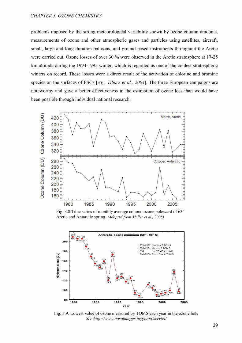
problems imposed by the strong meteorological variability shown by ozone column amounts,

measurements of ozone and other atmospheric gases and particles using satellites, aircraft,

small, large and long duration balloons, and ground-based instruments throughout the Arctic

were carried out. Ozone losses of over 30 % were observed in the Arctic stratosphere at 17-25

km altitude during the 1994-1995 winter, which is regarded as one of the coldest stratospheric

winters on record. These losses were a direct result of the activation of chlorine and bromine

species on the surfaces of PSCs [e.g., Tilmes et al., 2004]. The three European campaigns are

noteworthy and gave a better effectiveness in the estimation of ozone loss than would have

been possible through individual national research.

Fig. 3.9: Lowest value of ozone measured by TOMS each year in the ozone holeSee http://www.nasaimages.org/luna/servlet/

Fig. 3.8 Time series of monthly average column ozone poleward of 63o

Arctic and Antarctic spring. (Adapted from Muller et al., 2008)


30

3.13 Chemicals responsible for ozone destruction

The main free radical catalysts that can destroy the ozone layer are the hydroxyl radical (OH.),

the nitric oxide radical (NO.), atomic chlorine (Cl.) and atomic bromine (Br.) which have both

natural and anthropogenic sources. Presently most of the OH and NO in the stratosphere is of

natural origin while human activities have dramatically increased the atmospheric amounts of

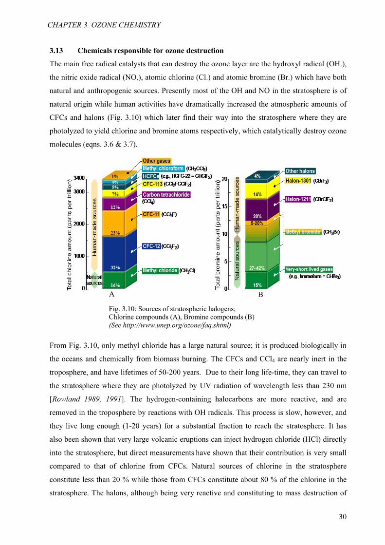
CFCs and halons (Fig. 3.10) which later find their way into the stratosphere where they are

photolyzed to yield chlorine and bromine atoms respectively, which catalytically destroy ozone

molecules (eqns. 3.6 & 3.7).

From Fig. 3.10, only methyl chloride has a large natural source; it is produced biologically in

the oceans and chemically from biomass burning. The CFCs and CCl4 are nearly inert in the

troposphere, and have lifetimes of 50-200 years. Due to their long life-time, they can travel to

the stratosphere where they are photolyzed by UV radiation of wavelength less than 230 nm

[Rowland 1989, 1991]. The hydrogen-containing halocarbons are more reactive, and are

removed in the troposphere by reactions with OH radicals. This process is slow, however, and

they live long enough (1-20 years) for a substantial fraction to reach the stratosphere. It has

also been shown that very large volcanic eruptions can inject hydrogen chloride (HCl) directly

into the stratosphere, but direct measurements have shown that their contribution is very small

compared to that of chlorine from CFCs. Natural sources of chlorine in the stratosphere

constitute less than 20 % while those from CFCs constitute about 80 % of the chlorine in the

stratosphere. The halons, although being very reactive and constituting to mass destruction of

Fig. 3.10: Sources of stratospheric halogens; Chlorine compounds (A), Bromine compounds (B)(See http://www.unep.org/ozone/faq.shtml)


A B

31

ozone, occur only in small quantities in the stratosphere (Fig 3.10). The Montreal protocol has

played a major role in enhancing the reduction of these compounds in the stratosphere (Fig

3.5).

3.14 Polar Stratospheric Clouds

Polar Stratospheric Clouds (PSCs) also known as the nacreous clouds are clouds that form in

the extremely cold and dry conditions (< -80oC), that exist in the polar night regions of the

stratosphere. PSCs are responsible for the Antarctic ozone hole in that they provide the

surfaces on which the heterogeneous reactions necessary for ozone destruction occur. PSCs

are divided into two classes, Type I and Type II, both of which are formed only under

extremely cold conditions that are found typically in the winter polar vortex region of the

Arctic and Antarctic stratosphere. They tend to form much more frequently in the more

isolated, colder Antarctic vortex, hence the existence of the ozone hole over there and not over

the Arctic. The temperature at which they form is referred to as the frostpoint.

3.14.1 Type I Polar Stratospheric Clouds (PSCs)

Type I PSCs are composed of a super-cooled liquid ternary solution of nitric acid, sulfuric acid,

and water ice (HNO3-H2SO4-H2O), as well as frozen Nitric Acid Trihydrates (NAT),

(HNO3.H2O). The frostpoint for Type I PSCs is (-78°C), and they are much smaller than Type

II PSCs, with particle diameter of < 1 μm and a sedimentation rate of the order of 0.01 km per

day.

3.14.2 Type II Polar Stratospheric Clouds (PSCs)

Type II PSCs are water ice particles that form when the temperature falls below (-85°C). They

are relatively large, with a diameter of < 10 μm, having a sedimentation rate of 1.5 km per day.

3.14.3 Heterogeneous reactions on the Polar Stratospheric Clouds (PSCs)

Heterogeneous reactions which refer to chemical reactions occurring in multiple states (gas,

liquid, and solid), are extremely important in the discussion of Antarctic ozone hole, since they

not only free chlorine and bromine from reservoir species into reactive forms but also help in

the removal of reactive nitrogen species (NOx) from the atmosphere by converting it to nitric

acid (HNO3), which prevents the newly formed ClO from being converted back into ClONO2.

Today, a variety of heterogeneous reactions of importance to stratospheric chemistry are

known with the most basic ones shown in reactions 3.20a-3.20h


32

The reaction rates of the above reactions depend on the particle type, particle surface area, and

temperature. During cold winter, reactions (3.20) increase dramatically, giving a better

understanding of the ozone budget of the polar stratosphere. Reaction 3.20a, proposed by

Solomon et al., [1986], converts the relatively stable chlorine reservoir species HCl and

ClONO2 into Cl2, thereby perturbing gas phase chlorine partitioning. Equally of importance

is (3.20e) [Molina et al., 1987], which is responsible for the activation of HCl and thus for a

complete activation of the stratospheric chlorine reservoir. Heterogeneous reactions on the

noncrystalline stratospheric sulfate aerosol were known to be important for mid-latitude

chemistry [e.g., Hofmann and Solomon, 1989], but were not thought to be of great relevance

for polar chlorine activation. Current studies have shown reaction probabilities of stratospheric

species on a variety of solid and liquid aerosol particles. These reaction probabilities are

frequently strongly temperature dependent being relevant only at low temperatures with the

exception of (3.20d), which is important at all temperature occurring in the stratosphere.

Reaction (3.20d) can take place whenever there is a particle in the stratosphere (e.g. after

volcanic eruption). It plays an important role in the explanation of nitrogen chemistry of the

middle latitude stratosphere. Molecules such as 2ClONO and HCl in reaction (3.20a) become

highly reactive with one another when dissolved in sulfuric acid-water but are non reactive in

their gaseous state, thus acting as chlorine reservoir species. The absorption of HCl and

ClONO2 on a liquid sulfate aerosol particle in the stratosphere results in the release of Cl2 and

the retention of a nitric acid (HNO3) molecule within the aerosol particle. The nonreactive

HNO3 formed remains in a solid (frozen) state on the surfaces of the PSCs. As the PSCs

undergo sedimentation, the HNO3 is carried out of the stratosphere. This process leads to the

removal of nitrogen from the stratosphere and is called denitrification. Since HNO3 photolysis

results in the formation of reactive NO2, which in turn reacts with ClO to form the reservoir

ClONO2 species, the removal of nitrogen from the stratosphere means that there is more

reactive, ozone destroying ClO. The chlorine species Cl2 and HOCl created in reactions


2 2 3

2 2 3

2 5 2 3

2 5 2 3

2 2

2 2 3

2 3

2

2

ClONO HCl Cl HNO

ClONO H O HOCl HNO

N O HCl ClNO HNO

N O H O HNO

HOCl HCl Cl H O

BrONO H O HNO HOBr

HCl BrONO HNO BrCl

HCl HOBr H O BrCl

(3.20a)

(3.20b)(3.20c)

(3.20d)

(3.20e)

(3.20f)

(3.20g)

(3.20h)

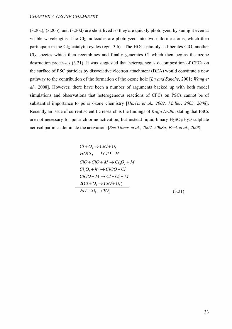
33

(3.20a), (3.20b), and (3.20d) are short lived so they are quickly photolyzed by sunlight even at

visible wavelengths. The Cl2 molecules are photolyzed into two chlorine atoms, which then

participate in the ClX catalytic cycles (egn. 3.6). The HOCl photolysis liberates ClO, another

ClX species which then recombines and finally generates Cl which then begins the ozone

destruction processes (3.21). It was suggested that heterogeneous decomposition of CFCs on

the surface of PSC particles by dissociative electron attachment (DEA) would constitute a new

pathway to the contribution of the formation of the ozone hole [Lu and Sanche, 2001; Wang et

al., 2008]. However, there have been a number of arguments backed up with both model

simulations and observations that heterogeneous reactions of CFCs on PSCs cannot be of

substantial importance to polar ozone chemistry [Harris et al., 2002; Müller, 2003, 2008].

Recently an issue of current scientific research is the findings of Katja Drdla, stating that PSCs

are not necessary for polar chlorine activation, but instead liquid binary H2SO4/H2O sulphate

aerosol particles dominate the activation. [See Tilmes et al., 2007, 2008a; Feck et al., 2008].

3 2

2 2

2 2

2

3 2

3 2

2( )

: 2 3

Cl O ClO O

HOCl ClO H

ClO ClO M Cl O M

Cl O hv ClOO Cl

ClOO M Cl O M

Cl O ClO O

Net O O

(3.21)


34

Chapter 4

4.0 Past ozone study

Since the discovery of the importance of atmospheric ozone, several measurements have been

carried out around the globe in order to understand the behaviour of the ozone layer and more

recently its depletion. The first set of measurements was ground based and later the balloon,

aircraft, rocket, and satellite borne instruments were used.

4.1 Ground based measurement of atmospheric ozone

During the study of meteors by Lindemann and Dobson in [1923] at Oxford University they

discovered that the temperature of the stratosphere increases with altitude, so they concluded

that the governing process in the stratosphere must be radiative and the temperature inversion

was due to UV radiation being converted into heat through ozone absorption which is in line

with Hartley’s prediction in 1881 [see Khrgian, 1975]. This discovery led to an increase in

ground based research into atmospheric ozone. Although the spectrograph designed by Fabry

and Buisson in 1921 was the first set of ground based instrument used to measure total ozone

column, it was soon superseded by that designed by Dobson in 1924, which was cheaper,

easier to build and allowed regular measurements to be made over extended time periods.

Other ground based instruments earlier used and some of which are still currently in use

include the M-83 ozone-meter and the M-124 filter ozone-meter, Umkehrs, and the Brewer

spectrophotometer. These instruments serve as the basis for validating satellite based ozone

measurements.

4.1.1 The Dobson spectrophotometer

The Dobson spectrophotometer is a double monochromator that measures the relative

intensities of pair wavelengths in the Huggins and Chappuis ozone band at wavelength ranges

of (300-350 nm) and (440-1180 nm) respectively, with a long-term ozone measurement

precision of 1% (for the 2 sigma level). The wavelength is chosen such that one is significantly

absorbed by ozone while the other is attenuated in the instrument by a calibrated optical

wedge. The wedge position is adjusted until equal signals for the two beams are obtained.

Measurements are made for two separate pairs of wavelengths to allow cancellation of errors

due to aerosols in the atmosphere [Dobson, 1957]. Daily measurements have been made using

a Dobson instrument at the station in Arosa, Switzerland, from 1926 to the present. Since 1957,

a network of more than 30 stations has been making measurements of the total ozone column.

This network is spread over much of the world but is heavily concentrated in the Northern

35

Hemisphere. The network of instruments is calibrated relative to a single world standard

instrument, which is itself calibrated each summer at Mauna Loa. The calibration is then

transferred to the rest of the instruments through secondary standard [Komhyr, 1989].

The standard unit for total atmospheric column of ozone is expressed in Dobson unit (DU),

which describes the thickness of a layer of pure ozone if the total amount of ozone in the

atmosphere were brought to standard conditions (293.15K and 1013hPa). For example, an

atmospheric ozone column of 300 DU brought down to the surface of the earth at 0oC would

occupy a 3mm thick layer of pure ozone. One DU is 2.69x1016 ozone molecules/cm2 or

2.69x1020 ozone molecules/m2. Although the instrument is primarily designed to measure

ozone total column it can also be used to find the vertical distribution of ozone. This technique

involves measurements at two wavelengths in the UV region at which ozone absorbs strongly

at one wavelength and weakly at the other wavelength. This can be explained by Lambert-

Beer’s law which defines the direct spectral irradiance Io(λ) reaching the Earth’s surface at

wavelength λ after attenuation by column amounts in the atmosphere with absorption cross

section σi(λ) by a particular atmospheric constituents having density n

Therefore the general relation for the calculation of total ozone from direct solar observation

can be determined from:

Taking the natural logarithm, we have

where Io(λ)/Io(λ)́ is known from measurement of solar radiation and ʃn(x)dx is the absorber

column amount along the effective light path, which is same as the slant column density. Direct

solar measurements are limited to daylight hours when the direct solar beam is not obscured by

clouds or other obstacles for a period of at least 2 min (Dobson) or 5 min (Brewer). The solar

zenith angles suitable for measurement for the different spectrophotometer differ and do not

exceed 72o for the Dobson and M-124 filter instruments, and 75o for the Brewer

Spectrophotometer due to the different wavelengths and temperature dependence for the

atmospheric constituent absorption coefficients. While the Dobson spectrometer measures

relative ratios of spectral irradiance at three wavelength pairs (A: 305.5/325.4; C: 311.5/332.4;

CHAPTER 4. PAST OZONE STUDY

'

( )( )exp ( ) ( )

( ') ( ')o

o

IIn x dx n x dx

I I

'

( )( )ln ln ( ) ( )

( ') ( ')o

o

IIn x dx

I I

(4.1)

(4.2)

(4.0)( ) ( ) exp( ( ) )oI I n x dx

36

D: 317.6/339.8nm), the Brewer spectrophotometer measure spectral irradiance at five

operational wavelengths (306.3, 310.1, 313.5, 316.8 and 320.1nm), and the M-124 filter

instrument measures at 302 and 326nm with the spectral band pass of 20 nm.

4.1.2 The Umkehr measurements

The Umkehr measurements are a sequence of special ozone measurements done from sunrise

to sunset using a spectrophotometer under clear skies and they provide atmospheric ozone

profiles at nine levels (0-49 km) with a systematic uncertainty or bias of about 15% to 20%,

which is based on the assumption that there are no ozone variations within each layer.

Currently a technique has been developed that enables 15 levels to be extracted from the data.

The Umkehr technique is based on the ratio of zenith sky radiances of two wavelengths in the

ultraviolet with one strongly and the other weakly absorbed by ozone, which increases with

increasing solar zenith angles but suddenly decreases at zenith angles close to 90o. This form

of measurements allow the deduction of a low-resolution vertical ozone profile [e.g., Paetzold

and Regener, 1957; Dutsch and Staehelin, 1992].

4.1.3 UV LIDAR systems

UV LIDAR systems developed in the 1980s as well as the microwave instrument operated

from the laboratory can be used to carry out measurements on and off the zenith sky through a

roof hatch or dome. LIDAR instruments must be located in such a way as to avoid interference

from other UV sources and can in some instances take measurements in other directions by

pointing the laser beam and detector to the direction of interest, but it is usually limited to

operating at night and when there is not an appreciable amount of cloud cover. This technique

which is similar to that employed by the Dobson spectrometer also involves measurements at

two wavelengths in the UV region at which ozone absorbs strongly at one wavelength and

weakly at the other wavelength.

4.1.4 Differential Optical Absorption Spectroscopy (DOAS) Measurement

The DOAS technique is a remote sensing method that is based on absorption spectroscopy in

the UV and visible wavelength range performed at moderate spectral resolution to identify and

separate different species. Long light paths can be obtained from the atmosphere by using

either sun or moon as the light source and even a longer light path can be realized at twilight

from scattered light. The scattered light observations can be taken at all weather conditions


37

without significant loss in accuracy for stratospheric measurements. The intensity measured by

the instrument which is weakened by absorption, Rayleigh and Mie scattering along the light

path is given by:

where a(λ,θ) is the scattering efficiency, Io(λ) is the unattenuated intensity, ( )j

s is the

concentration of trace gas j and ( )Mie

s and ( )Ray

s are concentrations of Mie and Rayleigh

scatterers, respectively. If the absorption cross-section does not vary along the light path s, then

the equation is simplified using the slant column1 (SC) given by:

inserting 4.4 into 4.3 yields

Since Rayleigh and Mie scattering efficiency vary smoothly with wavelength, they can be

approximated by low order polynomials.

4.2 Balloon and aircraft measurement of atmospheric ozone

The first attempt to directly measure the vertical profile of the atmospheric ozone concentration

was made by James Glaisher and Henry Tracey Coxwell on a manned balloon in

Wolverhampton, England on September 5, 1862. In the experiment, they used the Schönbein

method during which the balloon reached an altitude of 11 km but could only measure ozone

up to an altitude of 4.8 km before it lost consciousness at greater altitudes [Hoinka, 1997]. On

July 31, 1934 in Stuttgart, Regener and Regener (1934) carried out the first successful balloon-

borne measurements of the vertical distribution of ozone just after the first Umkehr

measurements. They recorded the solar UV spectrum in the stratosphere and deduced an ozone

profile from these measurements; with the data obtained from the measurement confirming the

first Umkehr observations. Balloon borne ozone sondes measure height–resolved profiles of

atmospheric ozone from the surface up to the 30-35 km range in the middle stratosphere and

can be operated in all climatic regions and under severe weather conditions. The sonde has a

reaction chamber where ozone molecules react with the chemical solution, an air pump, a

power supply, and an electronic interface that converts the raw current signal and transfers it to

the radiosonde. These components are mounted in a Styrofoam box in order to protect it from

1the total amount of the absorber per unit area integrated along the light path through the atmosphere

1

( , ) ( , ) ( ) exp ( ( ) ( ) ( ) ( ) ( ) ( ))oj j Mie Mie Ray Ray

N

j

I a I s s s ds

( )j j

SC s ds

(4.3)

(4.4)

1

( , ) ( , ) ( ) exp ( ) ( ) ( )o j Mie Mie Ray Ray

N

jj

I a I SC SC SC

(4.5)


38

low temperature effects and some mechanical impact. To transfer the ozone signal to the

ground receiver, the ozonesonde has to be connected to a suitable meteorological radiosonde

which transfers the ozone signal, along with meteorological parameters, to the ground station,

where all signals are decoded and recorded. The instrument is accurate because of its direct

measurement of atmospheric ozone. Also in the early fifties, Paetzold (1950) developed a

method for determining the vertical profile of ozone during lunar eclipses up to altitudes that

cannot be reached by balloons (about 45 km).

This method involves the determination of ozone profile from the ozone absorption in the

Chappius band measured at the edge of the Earth’s shadow on the moon [Paetzold, 1951]. The

first in situ measurement of an ozone profile above balloon altitudes was made on October 10,

1946 by a UV spectrograph mounted in a tail fin of an A4 rocket [Johnson et al., 1951].

Remote sensing observations with MW radiometers, DOAS spectrometers [Bruns et al., 2001]

and in-situ in photometers sampling the air in the troposphere and lower stratosphere

measurement [Wang et al., 2002] can also be performed from aircraft. The secondary ozone

maximum at about 90 km, which is an important feature of the vertical ozone profile was

discovered both in ozone measurements from rocket payloads and in ozone concentrations in

the upper atmosphere deduced from stellar occultation measurements made from a satellite

[Miller and Ryder, 1973; Hays and Roble, 1973]. In fact rocket measurements have been a

very important scientific tool in ozone measurement [e.g., Miller and Ryder, 1973; Vaughan,

1982, 1984; Gernandt et al., 1989].

4.3 Satellite measurement of atmospheric ozone

The first satellite measurements of the vertical distribution of ozone in the stratosphere and

mesosphere were made using the same technique similar to that of the lunar eclipse, but by

replacing the moon as a reflector by an artificial satellite [Venkateswaran et al., 1961]. Today,

several ways of measuring ozone from a satellite platform have been discovered, with each

method having its advantages and disadvantages. Many past studies on middle atmospheric

ozone employed satellite-based measurements in nadir-viewing geometry with e.g. the Global

Ozone Monitoring Experiment (GOME), the Total Ozone Mapping Spectrometer (TOMS) and

the Solar Backscatter Ultra Violet Instrument (SBUV), where each measurement displays a

little variation from the other. The measurements from GOME gave total ozone columns and

some other trace gases as well as vertical concentration profile of ozone with a low vertical

resolution (7-10 km) [Burrows et al., 1999]. This low vertical resolution does not provide

enough information for many scientific applications and the understanding of the stratospheric


39

chemistry and dynamics can mainly be achieved from observations with better altitude

resolution. Equally, measurements from SBUV [Heath et al., 1975] were capable of producing

global maps of the total ozone column with high spatial resolution, but the retrieved ozone

profiles have limited vertical resolution [e.g., Bhartia et al., 1996]. In this study, satellite-based

measurements done in limb and occultation viewing geometry were investigated. The limb-

viewing geometry gives a better altitude resolution with the line of sight (LOS) of a limb-

viewing detector being a tangential path through the atmosphere. The limb is scanned

vertically, and spectra are measured at different tangent altitudes, thus leading to a good

vertical resolution (2-4 km). Also in the limb-viewing geometry, the stratospheric optical depth

of the LOS is longer than in the nadir-viewing geometry, thus enabling greater sensitivity to

small amounts of stratospheric absorbers. The occultation viewing-geometry of satellite based

measurements is self calibrating and involves simple retrieval techniques, thereby providing

ozone density profiles with high vertical resolution, but suffers from poor geographical

coverage. In this study, the trend of stratospheric ozone was investigated with satellite

observations in the limb viewing geometry with the SCanning Imaging Absorption

spectroMeter for Atmospheric CHartographY (SCIAMACHY) (08/2002 – date) and in the

solar occultation viewing-geometry with the Stratospheric Aerosol and Gas Experiment II

(SAGE II) (10/1984 – 10/2005) and the Halogen Occultation Experiment (HALOE) (09/1991 –

11/2005) represented schematically in Fig. 5.0


40

Chapter 5

5.0 Instrument and theory

5.1 SCIAMACHY instrument

The SCanning Imaging Absorption spectroMeter for Atmospheric CHartographY

(SCIAMACHY) [Bovensmann et al., 1999] was launched on March 1, 2002 onboard the

European Environmental Satellite (Envisat-1) from Kourou, French Guiana. It makes nadir,

limb-scatter and occultation observations (Fig. 5.0). Envisat operates in a near-circular sun-

synchronous polar orbit having a mean altitude of about 800 km at an angle of inclination of

98o with a period of 100 min (about 14 orbits per day), moving with an orbital velocity of

approximately 7.45 km/s over ground crossing the equator on the descending node at about

10:00 local time. It always moves slightly against the rotation of the Earth and passes close to

the poles, having a repeated orbital cycle of 35 days with respect to the position of the Earth’s

surface and allows daily near-global measurements of the atmospheric composition from space

with a vertical resolution of 3-4 km [von Savigny et al., 2005b; Rozanov et al., 2005]. The

SCIAMACHY instrument was proposed in 1988 by the SCIAMACHY team [Burrows et al.,

1988] and funded by Germany, The Netherlands and Belgium. It is a UV, visible and

shortwave infrared, passive and moderate-resolution imaging remote sensing spectrometer

comprising 8 spectral channels covering a wide spectral range from 240-2400 nm and has a

spectral resolution between 0.24 nm and 1.5 nm, with each spectral channel having a grating

spectrometer with a 1024 element diode array as a detector. It achieves a full global coverage

in 6 days which results in a large amount of measured data requiring the operational retrieval

algorithms to be numerically efficient. Due to its well established measurement geometries,

high resolution and wide wavelength range, SCIMACHY is able to observe many different

trace gases despite their low concentrations (The mixing ratios of most constituents are of the

order of ppm or less). The large wavelength range is also ideally suited for the detection of

clouds and aerosols. The data obtained from SCIAMACHY can be applied in the area of

Global Monitoring for Environment and Security (GMES) which includes “Atmospheric

Monitoring”, Kyoto and Montreal Protocol verification as well as “Chemical Weather”

applications.

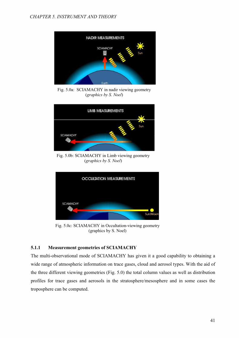
41

5.1.1 Measurement geometries of SCIAMACHY

The multi-observational mode of SCIAMACHY has given it a good capability to obtaining a

wide range of atmospheric information on trace gases, cloud and aerosol types. With the aid of

the three different viewing geometries (Fig. 5.0) the total column values as well as distribution

profiles for trace gases and aerosols in the stratosphere/mesosphere and in some cases the

troposphere can be computed.

Fig. 5.0a: SCIAMACHY in nadir viewing geometry(graphics by S. Noel)

Fig. 5.0b: SCIAMACHY in Limb viewing geometry(graphics by S. Noel)

)

CHAPTER 5. INSTRUMENT AND THEORY

Fig. 5.0c: SCIAMACHY in Occultation-viewing geometry(graphics by S. Noel)

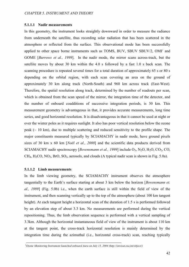
42

5.1.1.1 Nadir measurements

In this geometry, the instrument looks straightly downward in order to measure the radiance

from underneath the satellite, thus recording solar radiation that has been scattered in the

atmosphere or reflected from the surface. This observational mode has been successfully

applied to other space borne instruments such as TOMS, BUV, SBUV SBUV/2, OMI1 and

GOME [Burrows et al., 1999]. In the nadir mode, the mirror scans across-track, but the

satellite moves by about 30 km within the 4.0 s followed by a fast 1.0 s back scan. The

scanning procedure is repeated several times for a total duration of approximately 65 s or 80 s

depending on the orbital region, with each scan covering an area on the ground of

approximately 30 km along track (North-South) and 960 km across track (East-West).

Therefore, the spatial resolution along track, determined by the number of readouts per scan,

which is obtained from the scan speed of the mirror, the integration time of the detector, and

the number of onboard coadditions of successive integration periods, is 30 km. This

measurement geometry is advantageous in that, it provides accurate measurements, long time

series, and good horizontal resolution. It is disadvantageous in that it cannot be used at night or

over the winter poles as it requires sunlight. It also has poor vertical resolution below the ozone

peak (~ 10 km), due to multiple scattering and reduced sensitivity to the profile shape. The

major constituents measured typically by SCIAMACHY in nadir mode, have ground pixels

sizes of 30 km x 60 km [Noël et al., 2000] and the scientific data products derived from

SCIAMACHY nadir spectroscopy [Bovensmann et al., 1999] include O3, N2O, H2O, CO2, CO,

CH4, H2CO, NO2, BrO, SO2, aerosols, and clouds (A typical nadir scan is shown in Fig. 5.0a).

5.1.1.2 Limb measurements

In the limb viewing geometry, the SCIAMACHY instrument observes the atmosphere

tangentially to the Earth’s surface starting at about 3 km below the horizon [Bovensmann et.

al., 1999] (Fig. 5.0b) i.e., when the earth surface is still within the field of view of the

instrument, and then scanning vertically up to the top of the atmosphere (about 100 km tangent

height). At each tangent height a horizontal scan of the duration of 1.5 s is performed followed

by an elevation step of about 3.3 km. No measurements are performed during the vertical

repositioning. Thus, the limb observation sequence is performed with a vertical sampling of

3.3km. Although the horizontal instantaneous field of view of the instrument is about 110 km

at the tangent point, the cross-track horizontal resolution is mainly determined by the

integration time during the azimuthal (i.e., horizontal cross-track) scan, reaching typically


1Ozone Monitoring Instrument launched onboard Aura on July 15, 2004 (http://envisat.esa.int/object/)

43

about 240 km. However, in this study all spectra measured during the azimuthal scans will be

averaged to increase the quality of the input data, so as to achieve a cross-track resolution of

about 960 km. Other instruments that use this technique for measurement of atmospheric trace

elements are SME1, SOLSE2, and OSIRIS3. In this geometry, excellent spatial coverage, good

vertical resolution and continuous measurement of data can be achieved. It is only hindered by

its complex viewing geometry and poor horizontal resolution.

5.1.1.3 Occultation measurements

SCIAMACHY performs occultation measurements by using the elevation and the azimuth scan

mirrors similar to that of the limb mode. In this mode, the instrument tracks the sun or moon

during its rise or set behind the earth, thereby recording transmitted solar (or lunar) radiation

for different tangent altitudes (Fig. 5.0c). The main disadvantage of the occultation

measurements in general, is the limited spatial coverage, since the measurements in each orbit

are only performed during sunrise or sunset. Some other space borne instruments that have

been successfully used to measure trace gases as well as temperature and aerosol

concentrations in the Earth’s atmosphere using the solar occultation technique include the

Stratospheric Aerosol Measurement (SAM-II) [McCormick et al., 1979], the Stratospheric

Aerosol and Gas Experiments (SAGE I, II and III) [Chu and McCormick, 1979; Chu et al.,

1989; McCormick et al., 2002], the Halogen Occultation Experiment (HALOE) [Russell et al.,

1993a, 1993b], the Atmospheric Trace Molecule Spectroscopy (ATOMS) experiment

[Gunson, 1992], and the Polar Ozone and Aerosol Measurement (POAM II and III) [Glaccum

et al., 1996]. The occultation measurements are well suited for monitoring long-term trends in

atmospheric composition, because the measurement is self calibrating and relatively immune to

long-term instrument degradation. It also has high photon count rates due to the brightness of

the source (solar occultation), thus making it possible to achieve high signal-to-noise ratios

with a relatively small instrument field of view (FOV), which allows for a high vertical

resolution.

1Solar Mesosphere Explorer (explorer 64) launched onboard Delta 2914 on October 6, 1981(Thomas et al.)(http://lasp.colorado.edu/mission_history/)2Shuttle Ozone Limb Sounding Experiment launched onboard STS-87 on November 19, 1997 (http://en.allexperts.com/e/s/st/)3Optical spectrograph and Infrared Imager System launched onboard Odin on February 20, 2001(Llewellyn et al., 2003) (http://www.iac.es/project/OSIRIS/)


44

5.2 HALOE instrument

The Halogen Occultation Experiment (HALOE) was launched on September 12, 1991 onboard

the Upper Atmosphere Research Satellite (UARS) spacecraft at an inclination angle of 57o,

having an orbital period of 95.9 minutes. It started its science observations on October 11,

1991 after a period of outgassing. The HALOE instrument, being an occultation instrument is

self calibrating, highly stable, very sensitive with a vertical resolution of about 1.8 km and can

obtain 15 measurements during each sunrise/sunset by comparing the cold space spectra to the

obtained spectra. Its temporal coverage is similar to that of the SAGE missions. It measures the

vertical profiles of O3, HCl, HF, CH4, H2O, NO, NO2, aerosol extinction at 4 infrared

wavelengths, and temperature versus pressure with an instantaneous vertical field of view of

1.6 km at the Earth's limb. It has a global coverage of approximately 6 weeks, covering the

latitude range of 80° S to 80° N, making extensive observations of the Antarctic region during

southern spring. The altitude range of the measurements extends from about 15 km to 60-130

km, depending on the species, for example nitric oxide measurements extend through the lower

thermosphere. Ozone is derived from absorption bands in the thermal infrared region between

9.22 µm and 10.42 µm [Russell III et al., 1993]. Examples of pressure versus latitude cross

sections and a global orthographic projection for the September 21 to October 15, 1992, period

show the utility of CH4, HF, and H2O as tracers, the occurrence of desiccation throughout the

southern hemisphere, the presence of the water vapor hygropause in the tropics, evidence of

Antarctic air in the tropics, the influence of Hadley tropical upwelling, and the first global

distribution of HCl, HF, and NO throughout the stratosphere. Data used in this analysis are

from the HALOE V19 obtained from http://haloe.gats-inc.com/download/index.php. The

overall goal of HALOE is to provide global-scale data on temperature, ozone and other key

trace gases needed to study and to better understand the chemistry, dynamics and radiative

processes of the middle atmosphere and also to study the impact of CFCs on ozone using

hydrogen fluoride observations, in combination with other HALOE data.

5.3 SAGE II instrument

The Stratospheric Aerosol and Gas Experiment II (SAGE II) instrument was launched into a

57o inclination orbit on October 5, 1984 aboard the Earth Radiation Budget Satellite (ERBS)

[Mauldin et al., 1985]. It orbits around the earth in a non-sun-synchronous mode at about 650

km with a nodal period of 96.8 minutes. It was initially planned to be in orbit for 2 years but

was actually powered off on August 26, 2005, having measured for about 11years. It was later

succeeded by SAGE III, which was launched on December 10, 2001 onboard a Meteor-3M


45

spacecraft. SAGE II is aimed at providing data on the chemistry and dynamic motions of the

Earth's upper troposphere and stratosphere (10-40 km). It uses the solar occultation technique

to measure attenuated solar radiation throughout the 14 orbits per day (McCormick et al., 1989,

1992), in the Earth's limb utilizing seven channels centered at wavelengths ranging from 385 to

1020 nm, thereby observing in the Chappuis band centered at 600 nm for ozone. The exo-

atmospheric solar irradiance that is used in determining limb transmittances can also be

measured in each channel during each event. The measured sunlight, containing absorption

signatures by trace gases and aerosols, is converted into vertical profiles of ozone, water vapor,

nitrogen dioxide and aerosol extinction. The SAGE II instrument vertically scans the limb of

the atmosphere during spacecraft sunsets and sunrises (about 15 sunsets and 15 sunrises each

day). It was preceded by SAM II (Stratospheric Aerosol Measurement II), which has been

measuring 1.0 µm aerosol extinction in the polar regions since 1978, and SAGE I, which

provided near global measurements of aerosol extinction (at 0.45 and 1.0 µm), ozone, and

nitrogen dioxide from 1979-1981. Since the solar occultation technique is inherently self-

calibrating, accurate estimates can be made of long-term trends in the retrieved atmospheric

constituents to aid in assessing their role in global change. Both SAGE I and II satellites had a

low temporal and spatial coverage, tracking between typically 60◦ S and 60◦ N and obtaining a

global coverage within a month. The derived profile for each measured species is typically of 1

km vertical resolution with an altitude uncertainty of ~0.2–0.25 km from the surface to 70 km

(Chu et al., 1989).

5.3.1 Understanding the Antarctic ozone hole and PSCs with SAGE II measurements.

One of the important roles of measuring with SAGE II is in understanding the causes and

effects of the Antarctic Ozone Hole. SAGE II has been used to measure the decline in the

amount of stratospheric ozone over Antarctica since satellite measurements of the ozone hole

began in the early 1980s. With the help of the high resolution SAGE II measurements,

scientists were able to study the vertical structure of ozone in the Antarctic and, more

importantly, the correlations between various trace gases. In the past studies, SAGE II

measurements showed that the loss of water vapor in the region of depleted ozone was due to

the formation of Polar Stratospheric Clouds (PSCs). PSCs were first noted by a team of NASA

Langley scientists using another Langley satellite data set, Stratospheric Aerosol Measurement

II (SAM II). SAGE II measurements showed that PSCs were also present unusually far south

of the Arctic region during certain meteorological conditions, indicating that ozone destruction

similar to that over the Antarctic was possible at lower latitudes. A study of the SAGE I and


46

SAGE II data sets showed a decrease in ozone amount in the upper stratosphere over the high

latitudes of both hemispheres and in the lower stratosphere over most of the globe (Randal et

al., 1999). SAGE II has been the only occultation instrument that was able to show ozone loss

below 20 km globally.

5.3.2 Monitoring the effect of the Mt. Pinatubo volcanic eruption and water vapor

concentration using SAGE II measurements

SAGE II aerosol data have also been used to study the large-scale motions of the stratosphere.

After the volcanic eruption of Mt. Pinatubo in 1991, SAGE II measurements showed the

transport of volcanic aerosols across the entire tropical stratosphere and into the middle and

high latitudes in the months following the eruption [Trepte et al., 1993]. SAGE II aerosol

measurements have also been used to study cirrus clouds in the tropics which are important for

the understanding of cloud effects on global climate [Jensen et al., 1996]. Equally of great

importance is the study of water vapor in the atmosphere with SAGE II measurements

[Thomason, et al., 2004]. It is well established that atmospheric water vapor plays an

important part in the Earth's radiation balance, in many chemical cycles, and it can also be used

to trace the exchange of material between the upper and lower atmosphere [Schaeler et al.,

2009] SAGE II has provided chemical and climate modelers with several years of high

resolution water vapor measurements, which helps in better understanding of both the

chemistry and motion of the atmosphere. Studies are still continuing on how varying water

vapor concentrations can affect the global climate. By studying SAGE II water vapor profiles,

we can determine the long- and short-term effects of variable water vapor concentrations on

the temperature of the atmosphere.


47

Chapter 6

6.0 Variations in stratospheric ozone

During the measurement of ozone by Dobson in the 1920s, he observed that there was

variability in the ozone column amount both on a daily and seasonal basis. He noted that the

daily variability correlated with the passage of weather systems over the site of his

measurements. To investigate this variation, he distributed his instruments to a number of

places in order to carry out simultaneous measurements on a daily basis. In the analysis, he

discovered that there was a regular variation of the total column amount of ozone with the

weather systems. That is, the ozone amount anti-correlated with the air pressure, showing an

increase when the air pressure falls and a decrease when the air pressure rises. The interaction

of processes such as ozone production, loss, and transport that governs ozone variability

observed on different time scales helps to determine both the amount of ozone in the

stratosphere as well as its distribution with latitude, longitude and altitude [WMO, 1995, 1999].

The variations in the ozone amount based on short-term, seasonal, inter-annual and long-term

time scales are due to continuous motion in the atmosphere. In the lower atmosphere

(troposphere and lower stratosphere), ozone variability is chiefly due to the dynamical

(transport) process [WMO, 2003, Chipperfield, 2003] where ozone acts as a tracer of

atmospheric motion while in the upper stratosphere, the variability is mainly due to the

photochemical processes, which involves the creation and destruction of ozone [e.g. Garcia

and Solomon, 1983; Randall et al., 1995]. Ozone in the lower atmosphere has a longer lifetime

than ozone higher up because of the screening out of the ultraviolet radiation that drives ozone

photochemistry by the ozone higher up in the stratosphere.

6.1 Short-term variability

Short-term variability is used to describe the day-to-day and week-to-week variation in the

column amount of ozone due to the effect of the passage of the weather systems as in the lower

atmosphere or due to photochemical processes as in the upper stratosphere which could lead to

different effects such as diurnal variations, variations in solar ultraviolet radiation, temperature

driven variations, and particle precipitation events that originate from electromagnetic storms

on the sun.

48

6.1.1 Passage of the weather system

The transport of ozone in the lower atmosphere (troposphere and lower stratosphere) is

associated with the dynamics of motion in this part of the atmosphere. In the stratosphere, the

direction of flow of wind in the mid-latitudes is westerly during winter and easterly during

summer with the passage of a winter weather systems equivalent to the superposition of a

secondary air flow on top of the overall westerly flow. In addition to the overall flow of air, the

motion of individual air masses (advection) can be followed if we know the particular

temperature, moisture content, and amounts of the trace gases (e.g., ozone) in different air

masses. The motion of air in the troposphere and stratosphere is driven by pressure gradients.

In a high pressure region, the air in the tropospheric column sinks downward thereby resulting

in the compression and heating of the air but above the tropospheric high pressure system, the

air rises and settles in the stratospheric column near the bottom of the stratosphere and is later

removed from the column at higher altitudes [Narayana et al., 2003]. Since the ozone mixing

ratio in the lower stratosphere increases with increasing altitude, the air brought into this

column has less ozone than the air being removed, thereby leading to a decrease in the amount

of ozone in the column, thus accounting for the decrease in ozone amount within the high

pressure region. The opposite is the case with a low pressure region where the ozone amounts

are increased. These variations only lead to temporary redistributions of ozone with no net gain

or loss. The slowness of the photochemical reaction in the lower stratosphere is the reason why

transport processes are responsible for most of the observed variations in lower stratospheric

ozone with a decrease in a high pressure region balanced by an increase in surrounding

regions.

6.1.2 Diurnal variation

The daily variation in the amount of ozone in the upper stratosphere (above 40 km) is due to

the reduction in the photochemical replacement time (PRT) as a result of low amount of ozone

in the region [Tuck, 1977, Herman, 1979, Groves and Tuck, 1980 Pallister et al., 1983].

During the day, UV radiation of wavelength less than 240 nm splits apart oxygen molecules to

form atomic oxygen, which then rapidly reacts with another O2 molecule to form ozone. After

sunset, the photolysis of O2 is shut off, and all the available O atoms are converted to ozone

molecules in three body reactions that occur at a very fast rate. As the Sun rises, some of the

ozone molecules are broken down by UV radiation at wavelengths less than 320 nm and some

also react with O atoms to reform oxygen molecules (3.1d). Both the photolysis of O2 (3.1a)

and the reaction of O with O3 (3.1d) are relatively slow processes compared to O3 photolysis

CHAPTER 6. VARIATIONS IN STRATOSPHERIC OZONE

49

(3.1c) and the reaction of O with O2 molecules (3.1b). At altitude of 40 km, there is not much

daily variation in the amount of ozone during the day as there is a balance between production

and loss in ozone but when the sun sets, both production and loss are turned off.

6.1.3 27 day solar rotation

The sun rotates with a 27-28-day period, so the ultraviolet radiation from the sun is modulated

by this rotational period. Occasionally, two active sunspot regions occur on opposite sides of

the sun thereby leading to a 13-day modulation of ultraviolet radiation which directly affect

ozone photochemistry and even the ozone column amount [DeLand and Cebula, 1998]. The

photolysis of O2 and O3 leads to the production of atomic oxygen which can either react

directly with O3 or with any of the oxides of hydrogen, nitrogen, chlorine, and bromine (3.5-

3.10). Thus, the photochemical reaction at the upper stratosphere leads to variations in the

photolysis rate of O2 and O3.

6.1.4 Variation in temperature

Although the upper stratosphere is dominated by photochemical production and loss processes,

dynamical variations also produce short-term variations. Planetary waves propagating upward

from the lower atmosphere grow in magnitude as altitude increases thereby leading to

variations in temperature which then affect the photochemical reaction rates, because the

reaction rate coefficients that determine photochemical loss rates are temperature dependent.

As mentioned above, the effect of temperature on ozone photochemistry is not only restricted

to pure oxygen reaction but also has effect on catalytic reactions involving various oxides of

nitrogen, hydrogen, chlorine, and bromine (3.5-3.10). The nitrogen oxide catalytic cycle has a

similarly strong dependence on temperature as the pure oxygen case while the hydrogen,

chlorine, and bromine oxide catalytic cycles each have much weaker temperature dependence.

The temperature dependence on ozone photochemistry is such that the loss rate increases with

increasing temperature. This means that ozone amounts will decrease when temperatures

increase and are thus anti-correlated with temperature. This effect becomes strongest during

winter when wave activity propagating into the stratosphere is strongest [Singleton et al.,

2005].


50

6.1.5 Solar proton events

Solar storms lead to ejection of large amounts of high energy protons that can penetrate the

Earth's magnetic field near the poles [Mewaldt et al., 2005]. These protons penetrate into the

atmosphere, typically up to the 40 to 80 km layer, causing ionization of air molecules. As the

ionized constituents recombine, they produce nitrogen and hydrogen oxides which can affect

ozone through the NOx [Garcia and Solomon, 1994, Crutzen, 1970, 1971] and HOx [Bates and

Nicolet, 1950] catalytic cycles. For the HOx catalytic cycle, the effects are short lived because

the hydrogen oxides which cause the primary ozone loss recombine within hours whereas the

effects of nitrogen oxides can persist for several months.

6.2 Seasonal variability

In the upper stratosphere, the seasonal variability of ozone concentrations is driven by the

seasonal variation of solar UV intensity, where during the late summer months ozone maxima

occur due to an enhanced photochemical production [Brasseur and Solomon, 1984], but in the

lower stratosphere, photochemistry is much slower, owing to reduced UV flux, so transport of

ozone by large-scale atmospheric motions becomes important [Newman et al., 2001]. The mid-

latitude total column ozone exhibits a strong seasonal variation which is at its maximum in late

winter or early spring and at minimum in late fall [Rood et al., 2000]. The primary driver of the

springtime maximum in total ozone is the transport of ozone rich air from the tropics towards

the poles during winter when the photochemical time constant for ozone is long because of

effective shielding of ozone in the lower stratosphere by ozone above and also because the

solar angle becomes low at high latitudes during winter. But the question now is why is ozone

transported to the poles during winter? This is because the primary circulation of the lower

stratosphere driven by the dissipation of wave disturbances propagated upward from the

troposphere is upward in the tropics and downward/poleward at the mid and high latitudes

[Cooper et al., 2005]. This large-scale wave (Rossby waves) disturbance with a spectrum of

spatial and temporal scales generated in the troposphere by flow over mountain ranges and

across the temperature contrast of land-sea interfaces is filtered in the stratosphere with only

the larger scale waves propagating westerly into the stratosphere during winter. But as summer

approaches the solar angle increases and also the large-scale waves stop propagating into the

stratosphere as the direction of the wind in the stratosphere becomes easterly thereby leading to

a decrease in the ozone concentration which gets to a minimum during late fall and picks up

again when winter returns.


51

6.3 Inter-annual variability

Inter-annual variability corresponds to the variation in the annual distribution of the ozone

amount which could be regular such as the Quasi Biennial Oscillation (QBO) or irregular such

as in The El Niño-Southern Oscillation (ENSO), the 11-year solar cycle and volcanic eruption.

6.3.1 Quasi-Biennial Oscillation (QBO)

The Quasi-Biennial Oscillation is a reversal of the regular west-east winds in the tropical

stratosphere that occurs approximately every 26 to 30 months [Baldwin et al., 2001], due to the

vertical propagation of waves from the tropical troposphere into the lower stratosphere. The

QBO does not only change the circulation in the tropics, it also indirectly causes changes at the

middle and high latitudes [Fleming et al., 2002]. This variation in the propagation speeds of the

extra-tropical waves also strengthens the Brewer-Dobson circulation. During the late winter

months, when the Brewer-Dobson circulation is at its strongest, air from the tropics is

transported towards the winter pole, which accounts for the large ozone concentration

increments in the middle and lower stratosphere [Hasebe, 1980; Bowman, 1989].

6.3.2 The El Niño-Southern Oscillation (ENSO)

ENSO is a global event that arises from large-scale interaction between the ocean and the

atmosphere, leading to large variations in equatorial Pacific Ocean surface temperatures within

a period of 4-7 years between episodes. Normally, the waters of the Eastern Pacific Ocean near

South America are quite cool as a result of upwelling ocean currents due to east to west

transverse of the tropospheric trade wind in this region. However, in an El Niño period, the

trade winds weaken, allowing the warmer waters of the Western Pacific to migrate eastward.

This change in sea surface water temperature causes large-scale shifts in the global circulation

patterns in the troposphere and lower stratosphere which equally affects the transport of ozone

in these regions. There is a strong relationship between ENSO and variability in the southern

hemisphere general circulation features [Shiotani, 1992, Zerefos et al., 1992]. During La Nina

the polar vortex is stronger and displaced more off the pole, the ozone croissant1 (OC) becomes

very strong between 40-60oS, and there are more PSCs and lower temperatures in the polar

vortex above 16 km while during El Nino the polar vortex becomes weaker, more centered on

the pole, midlatitude ozone is arranged in rings, and there are fewer PSCs and warmer

temperatures in the polar vortex above 16 km [Collimore et al., 2003]. This interannual

variability is in contrasts with the strong longitudinally-focussed outflow from Indonesia

during La Nina with the more longitudinally-extensive outflow events during El Nino.


1Ozone contour shape of monthly mean ozone around 50oS between May and November

52

6.3.3 Volcanic eruptions

Explosive volcanic eruptions [Altorio et al., 1992, Beig et al., 2002, Stenchikov et al., 2002]

can inject large amounts of material such as chlorine, sulfur dioxide (SO2) and some other

compounds directly into the lower stratosphere which affect the content of ozone in the

stratosphere. The ejected chlorine, although in minor proportion, enhances the catalytic

destruction of ozone, while the SO2 is converted to sulfate aerosol which provides the catalytic

surface on which nitrogen and chlorine are converted from reservoir species to active form that

begins the ozone destruction process.

6.3.4 11-year suns spot cycle

The output of solar ultraviolet radiation is influenced by magnetically active regions on the sun

that occur intermittently in sunspots (cooler regions on the sun) during which the UV output

increases as the sunspot activity increases. The sunspots occur in a quasi-regular 11-year cycle

and the period of the greatest sunspot activity during the 11-year cycle is called the solar

maximum at which certain wavelengths of UV radiation are enhanced due to the occurrence of

numerous active regions, while the period when sunspot activity is at its least is a solar

minimum at which the active region and the 27 day cycle disappears and the solar UV

radiation comes to a minimum [Angel, 1989, Hood and McCormack, 1999]. The effect of

sunspots on solar ultraviolet radiation output depends strongly on the particular wavelength of

ultraviolet radiation [Dessler et al., 1998] and it occurs in clusters on one side of the sun during

solar maxima.

6.4 Long-term variability

This is the variations with time scales typically on the order of decades which are due to a

trend or gradual build-up in the amount of ozone-destroying substances in the stratosphere. The

most important influence on the long-term variability of stratospheric ozone is the introduction

of significant amounts of chlorine into the stratosphere from anthropogenic

chlorofluorocarbons (CFCs) (see page 21). In order to determine any long-term ozone trend

we need to remove the cyclic variations in ozone and check whether or not the data set is long

enough to determine the difference between real and cyclic variations with periods longer than

the data set since some unknown factors that can contribute to a variation with a period longer

than the period of our record might cause us to conclude erroneously about the existence of a

long-term trend in the data [Newchurch et al., 2003, Steinbrecht et al., 2003, 2006]. To be


53

certain that there are no major unresolved long-term variations such as the solar activity we

need to understand all of the observed variations and attribute them to physical processes.


54

CHAPTER 7.

7.0 Results and discussion

7.1 Determination of the monthly mean

To analyze the trend of ozone, the monthly profiles from each of the satellite instruments were

formatted on the same altitude grid and grouped into altitude and latitude bins. The considered

altitude bins are 20–25 km, 25–35 km, and 35–45 km, while the considered latitude bins are

60◦ S–30◦ S, 30◦ S–30◦ N, and 30◦ N–60◦ N. The essence of the choice of these latitude and

altitude bins was to avoid some uncertainties. For example, below 20 km there are retrieval

issues in some data sets due to heavy levels of aerosol loading, atmospheric variability (strong

seasonal variation in trends over the northern mid-latitudes during winter and spring) and

Rayleigh scattering effects. While above 45 km, much care is needed in order to account for

large non negligible diurnal variability in ozone. Also, the choice of latitude bins from 60oN to

60oS was made in order to avoid the use of profiles that may be situated inside the winter polar

vortices where the concentration of ozone may be low. To remove unrealistic or erroneous

profiles, SAGE II data sets were screened by excluding profiles that were flagged for high

aerosol optical depth at 1020 nm (mostly the period after the 1991 Pinatubo eruption) thereby

showing unrealistically high ozone values or a failure of the ozone retrieval routine [see Rind et

al., 2005]. For the SCIAMACHY and HALOE data sets no additional screening seemed

necessary but only unrealistic spikes in the HALOE error estimates were removed. The zonal

mean monthly mean profiles for each of the instruments were obtained by averaging all

satellite profiles in each of the nine altitude/latitude bins (eqn. 7.0). This was done in order to

reduce measurement error or noise from the different instruments and the plots of the resulting

profiles are shown in Fig 7.0.

Where i, j are the altitude/latitude indices, k is the month index, N is the number of profiles in a

given month, and M is the ozone concentration.

, ,

( , , )( )1

1i j k

i j kmean nnijk

NM M

N

(7.0)

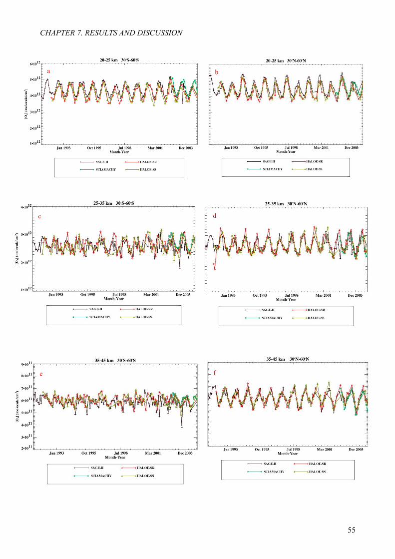
55

a b

e

c d

f

CHAPTER 7. RESULTS AND DISCUSSION

56

The monthly mean plots for all instruments (Fig. 7.0) show the time series of SCIAMACHY in

green, HALOE SR in red, HALOE SS in yellow-green and SAGE-II in black. The plots show

quite good agreement between all three instruments within the chosen altitude and latitude

bins. Although the SCIAMACHY instrument measurements were for a short period of time,

the other two instruments show good agreement. When the SAGE II and HALOE data sets

were compared at the tropics between October 1991 and March 2004 (Fig 7. 0 (g, h, i)), there

was a noticeable decrease of ozone till about 1997 especially at the mid-latitudes from 35-45

km. Although data was filtered for aerosol artifacts, large values of these artifacts still appear

to persist in SAGE II data especially in the 20-25 km altitude bin (Fig 7.0g) where there were

occasional large mean monthly values, so some of the values that showed unrealistic values for

ozone concentration from the instrument mostly between 1991 and 1994 were removed. It is

Fig 7.0: The monthly mean ozone concentration averaged over different altitude and latitude bins

i

g h


57

also observed from the plots that the ozone concentrations in the northern hemisphere are

higher than those in the southern hemisphere with each of the individual time series having

some variability. Moreover, the seasonal variation in ozone concentrations is more pronounced

in the northern hemisphere compared to the southern hemisphere, particularly for the 35–45

km altitude bin. So in summary it has been established that the monthly means from each

instrument are generally consistent with each other with low biases during overlapping periods.

7.6 Determination of ozone anomalies

Some of the variations observed in the individual time series are cyclic in nature associated

mainly with the seasonal, QBO and solar cycles, were the main contribution is due to seasonal

variation. To remove the seasonal variation from the individual zonal mean monthly mean

profiles, a similar approach adopted by Newchurch et al. [2003], Steinbrecht et al.[2004, 2006,

2009] and Jones et al. [2009], was carried out, in which the monthly ozone anomalies were

calculated by first removing the annual cycle. This was done for each of the instruments by

finding the difference between each monthly mean value from their corresponding average

(climatological) annual cycle. For example, in the calculation of the SAGE II anomalies, the

annual cycle was first calculated by computing the mean of a particular month (e.g. January

mean value calculated from all January from 1984-2005). This computed mean was later

subtracted from each individual SAGE II January mean concentrations (eqn. 7.1). Although the

anomalies obtained still have some fluctuations associated with the QBO and solar cycles, the

contributions of these processes are not so large in the region of interest (35-45 km).

where A(cycle) is the average annual cycle and i is the particular month within the period (Jan.-

Dec.). The anomalies were calculated individually for all the three instruments data sets on all

altitude and latitude bins so as to remove systematic biases between individual data sets. The

plot of the anomaly from the individual instrument (Fig. 7.2), the grouped all instruments

anomalies (Fig. 7.3) and the smoothed anomalies (Fig. 7.4) show a good trend of ozone and

instrument agreement.

( , , ) ( , , ) ( , , )( ) ( ) ( )i j m i j m l i janomaly mean cycleM M A (7.1)


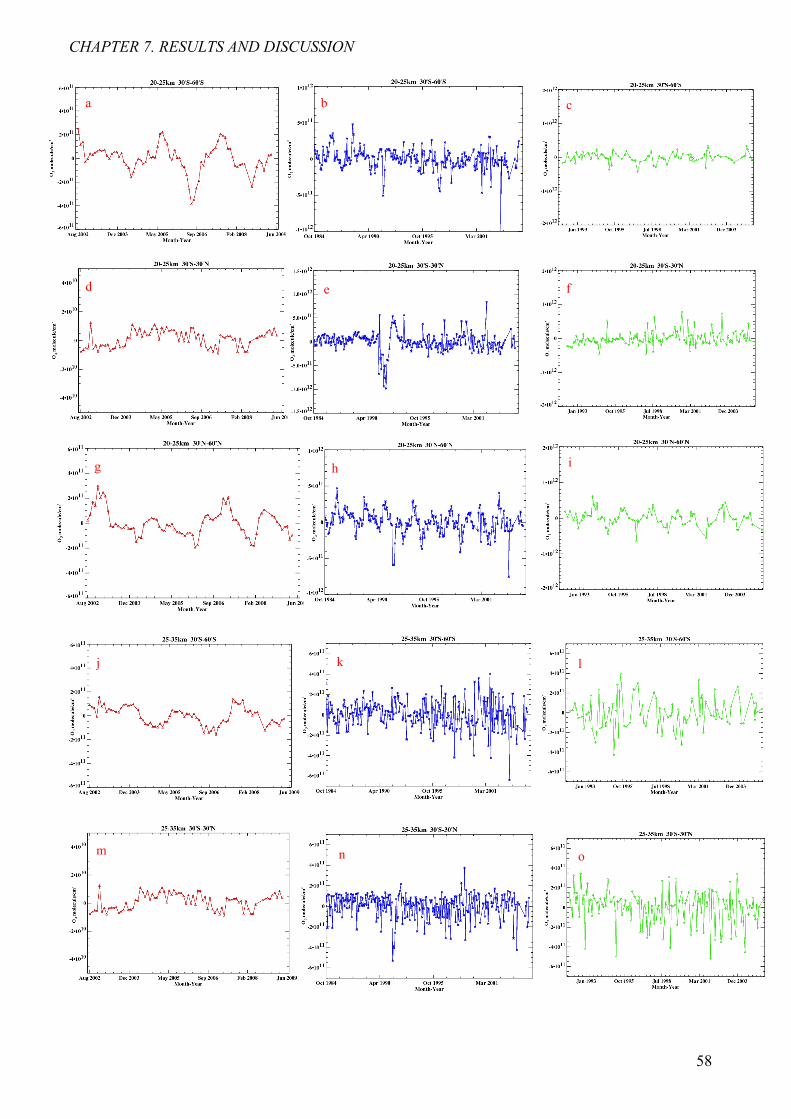
58

a b c

d e f

g h i

j k l

m n o


59

Fig 7.1 Ozone anomaly from the different instruments for different altitude and latitude bins; SCIAMACHY (left panel), SAGE II (middle panel), HALOE (right panel)

p q r

s t u

w xv

y z aa


60

Fig 7.1 shows the ozone anomaly from each of the three instruments at the nine

altitude/latitude bins. The anomalies from the SAGE II instrument (middle panel in blue)

which covers a longer time period than all the three instruments shows a clear variation in the

amount of ozone mostly at the 35-45 km altitude bin at all the considered latitude bins (Fig 7.1

t, w, z), such that within this altitude bin we can already identify evidence of recovery or at

least stagnation of the decrease of ozone. In the 20-25 km altitude bin for latitudes within 30oS-

30oN (Fig 7.1e), there was a sharp decrease in the ozone amount around 1991 after the Mount

Pinatubo eruption. The mid-latitudes of the lower stratosphere at both the Northern and

Southern hemisphere, measurement from SAGE II also showed declines of up to 10 % by 1995

between 35 and 45 km altitude but this decrease is no longer evident in the last decade

[Steinbrecht et al., 2009 , Jones et al., 2009] .

Fig 7.2: Ozone anomaly from all three instruments


a b

cd

ef

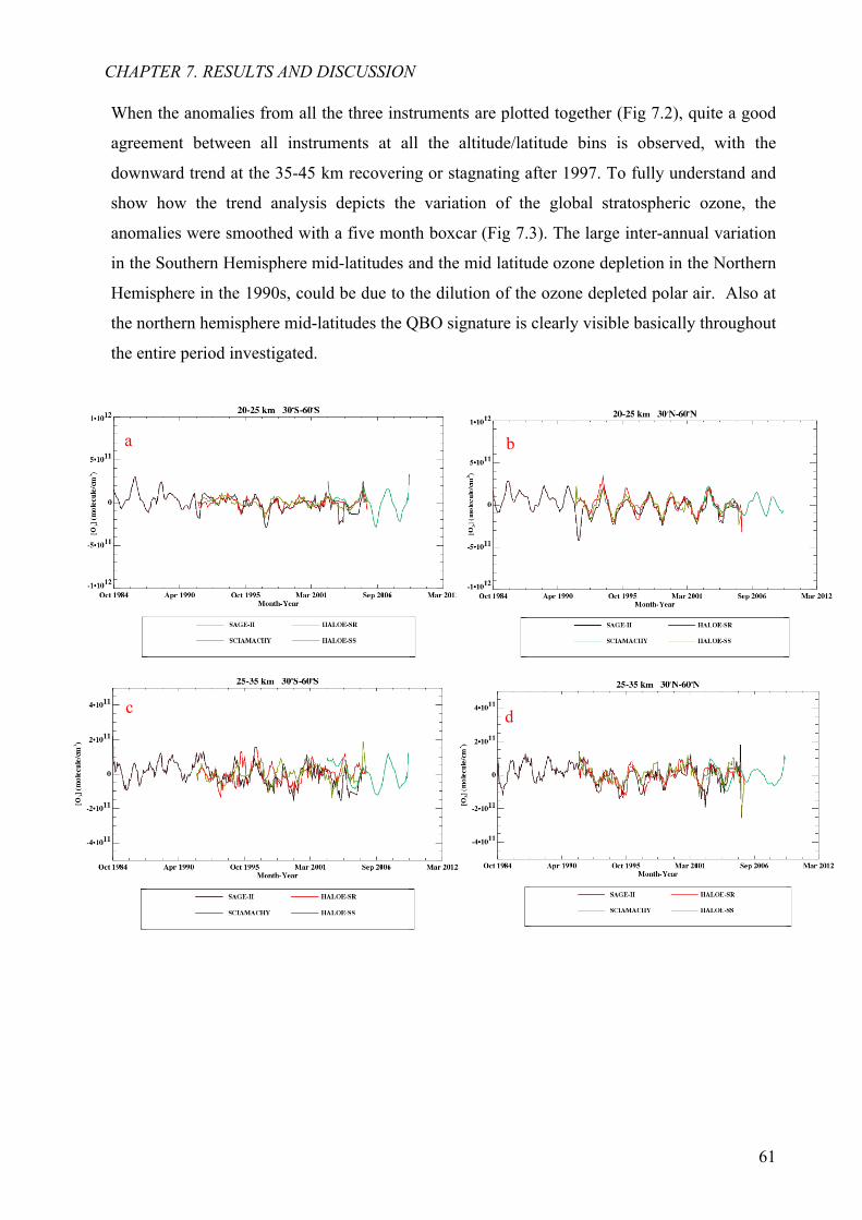
61

When the anomalies from all the three instruments are plotted together (Fig 7.2), quite a good

agreement between all instruments at all the altitude/latitude bins is observed, with the

downward trend at the 35-45 km recovering or stagnating after 1997. To fully understand and

show how the trend analysis depicts the variation of the global stratospheric ozone, the

anomalies were smoothed with a five month boxcar (Fig 7.3). The large inter-annual variation

in the Southern Hemisphere mid-latitudes and the mid latitude ozone depletion in the Northern

Hemisphere in the 1990s, could be due to the dilution of the ozone depleted polar air. Also at

the northern hemisphere mid-latitudes the QBO signature is clearly visible basically throughout

the entire period investigated.


a b

c d

62

7.2.1 Offset Corrected anomalies

To minimize the difference between the individual anomalies and align those that overlap in

time, we performed an offset correction (Fig 7.4). One important factor for the method to work

is that each individual data set must overlap with at least one other data set within an overlap

period of typically a couple of years. As the primary aim of this thesis is to investigate the

trend of stratospheric ozone, special focus was placed on the 35–45 km altitude bin, since it has

been confirmed that the largest estimates of ozone loss (6–8%/decade) occurs in the upper

stratospheric mid-latitudes, typically between 35–45 km [Newchurch et al., 2003; Steinbrecht

et al., 2003, 2004; Cunnold et al., 2004], due to the efficiency of ClOx catalytic ozone

destruction at this altitude bin. So it was considered important first to check the effect of a

reduction in the stratospheric chlorine loading on ozone destruction. To correct the offset

biases for each of the instruments time series, the mean ozone concentration was determined

for the period of January 2003 to August 2005 (for which measurements from all three

instruments are available) and the derived differences between SAGE and HALOE, as well as

SAGE and SCIAMACHY were used to correct the HALOE and SCIAMACHY time series

such that the mean concentration for the period mentioned above were identical for all 3

instruments. The average value (green plot in Fig 7.4) for all observational data sets shows a

good correlation with the individual data sets. In addition to the satellite data sets used, the

monthly mean ozone profiles from multi-year simulations of twelve state-of-the-art chemistry-

climate models were used. These runs which is part of the Chemistry Climate Model

Validation initiative [CCMVAL, http://www.pa.op.dlr.de/CCMVAL/, Eyring et al. 2006, WMO

2007], has all simulations which assumed increasing source gases (CO2, N2O, CH4, and CFCs),

Fig 7.3: Smoothed ozone anomalies from all three instruments

e f

63

realistic sea-surface temperatures, 11-year solar-cycle and QBO. From the CCMVal runs, the

zonal mean monthly mean ozone anomalies at the altitude and latitude bins of 35-45 km and

30o-60o respectively on both hemispheres over the period of 1984–2009 were considered.

These Anomalies were averaged over all models to form a multi-model mean, which was

further smoothed by a 24 month running mean. This running mean, together with the ±2

standard deviation (gray underlay plot in Fig 7.4c, d) of all modeled monthly mean anomalies

over the 24 month window, gave a good representation of the range of upper stratospheric

ozone anomalies simulated by the CCMVal models.

Fig 7.4: Combined and offset corrected anomalies; No CCMVAL model simulations plot (a, b), CCMVAL model simulations plot (c, d)

dc

a b

64

7.3 Turn around event

Lastly, the ozone trends in each latitude/altitude bin was estimated [Reinsel et al., 2002a, Jones

et al., 2009] using the assumption that if there is a change in trend, the trend line will be both

linear and continuous Reinsel et al. [2002a]. As it has been suggested that a turn around point

for ozone occurred sometime between 1995 and 1997 due to the recorded declines of HCl and

HF concentrations, in our analysis we assume that the turn around or break point year in the

ozone trend occurred in January 1997 [Steinbrecht et al., 2006, WMO, 2006, Newchurch et al.,

2003, Cunnold et al., 2004, Jones et al., 2009]. It is most likely that this turn around point will

be firstly seen in the upper stratosphere where halogen compounds responsible for ozone

destruction are broken down by strong UV light [Jucks et al., 1996] and should also be later

observed in the lower stratosphere as the halogen gases are slowly phased out. This particular

date is thought to be the nearest whole year when equivalent effective stratospheric chlorine

(EESC) reached its peak before its slow decline in the extra-tropical lower-middle stratosphere

based on a 3 year time lag of mean aged air [Newman et al., 2007]. However, an assumption

that 1997 is the turn around time for all latitudes and altitudes may not be fully established as

there are variations in dynamics and chemistry with time and space thus implying that the turn

around time may differ. A careful section of this turn around point is necessary as a shift in the

turn around year by just one year or even a few months can give vast differences in trend

magnitude both before and after this defining time. Several attempts have been made to

accurately define a turn around time using only ozone time series. This includes a linear trend

that is continuous [Reinsel et al., 2002a] and a non linear trend using the cumulative sum

(CUSUM) method [Reinsel et al. (2002b) as well as Newchurch et al. (2003), and Yang et al.

(2006]. The CUSUM method investigates how the anomalies deviate from the extrapolated

trend line while a change in the linear trend characterizes an explicit temporal path. CUSUM

studies suggest that the turn around time is typically around the end of 1996 for northern mid-

latitudes and from the tropopause up to 45 km. Calculations suggest that a change from a

negative trend to a less steep trend or positive trend can take a few years, but does include a

linear trend prior to and after the turn around period. So our choice of the linear trend appeared

justify although in our analysis we saw that the turn around point occurred earlier than 1997.

An easy way to analyze the linear trend method is to use a chi square or maximum likelihood

test, which examines the white noise before and after the break date, where the year with

smallest χ2 value indicates the closest time to a possible break in trend. This is justified as we

expect smaller stochastic errors when the residuals are closest to the trend model.

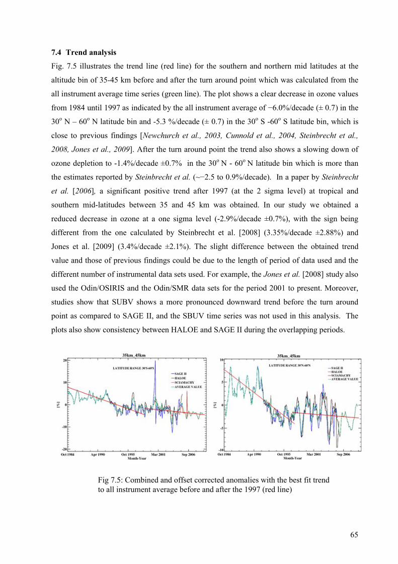
65

7.4 Trend analysis

Fig. 7.5 illustrates the trend line (red line) for the southern and northern mid latitudes at the

altitude bin of 35-45 km before and after the turn around point which was calculated from the

all instrument average time series (green line). The plot shows a clear decrease in ozone values

from 1984 until 1997 as indicated by the all instrument average of −6.0%/decade (± 0.7) in the

30o N – 60o N latitude bin and -5.3 %/decade (± 0.7) in the 30o S -60o S latitude bin, which is

close to previous findings [Newchurch et al., 2003, Cunnold et al., 2004, Steinbrecht et al.,

2008, Jones et al., 2009]. After the turn around point the trend also shows a slowing down of

ozone depletion to -1.4%/decade ±0.7% in the 30o N - 60o N latitude bin which is more than

the estimates reported by Steinbrecht et al. (~−2.5 to 0.9%/decade). In a paper by Steinbrecht

et al. [2006], a significant positive trend after 1997 (at the 2 sigma level) at tropical and

southern mid-latitudes between 35 and 45 km was obtained. In our study we obtained a

reduced decrease in ozone at a one sigma level (-2.9%/decade ±0.7%), with the sign being

different from the one calculated by Steinbrecht et al. [2008] (3.35%/decade ±2.88%) and

Jones et al. [2009] (3.4%/decade ±2.1%). The slight difference between the obtained trend

value and those of previous findings could be due to the length of period of data used and the

different number of instrumental data sets used. For example, the Jones et al. [2008] study also

used the Odin/OSIRIS and the Odin/SMR data sets for the period 2001 to present. Moreover,

studies show that SUBV shows a more pronounced downward trend before the turn around

point as compared to SAGE II, and the SBUV time series was not used in this analysis. The

plots also show consistency between HALOE and SAGE II during the overlapping periods.

Fig 7.5: Combined and offset corrected anomalies with the best fit trend to all instrument average before and after the 1997 (red line)

66

7.5 Summary

The long-term evolution of ozone was examined on nine latitude/altitude bins covering 60o S

and 60o N and 20-45 km respectively. Seasonal variability was removed from each of the

instruments monthly mean time series and the remaining residual from all the individual

instrument were combined in order to construct a weighted all instrument mean. Each of the

individual satellite monthly mean time series show generally a good agreement with systematic

biases typically less than 10% during overlapping periods. For the two latitude bins considered

during the assumed turn around point of 1997, significant trend was observed similar to those

reported by the WMO [2006]. The decline observed at the southern hemisphere between 35-45

km (-5.3 %/decade ± 0.7) is lower than that observed in the northern hemisphere

(−6.0%/decade ± 0.7). After 1997, it was found that in both hemispheres considered, the

decline has slowed down. If ozone continues to increase at the current rate for these specific

bins then pre 1980 values would be reached in approximately 60 years.

Finally, although the all instrument average can provide a more precise estimate of trend as it

can combine differing time domains as well as reduce the stochastic noise from individual data

sets, a better trend analysis can only be made if the residual time series is long enough and is

characterized by low residual noise, and low variability. Shorter time series is also necessary

as they have little long-term drift. As current ozone levels are typically 10–12% lower than pre

1980 values in the upper extra-tropical stratosphere, it take quite a long time before it can reach

the pre 1980 values as our post 1997 trend gave negative trend on both hemispheres.

67

REFERENCES

Anderson, J., J. M. Russell III, S. Solomon, and L. E. Deaver, Halogen Occultation Experiment confirmation of stratospheric chlorine decreases in accordance with the Montreal Protocol, J. Geophys. Res., 105(D4), 4483–4490, 2000.

Angel, I. K., On the relation between atmospheric ozone and sunspot number, J. Clim., 2, 1404-1416, 1989.

Baldwin, M. P., Gray, L. J., Dunkerton, T. J., Hamilton, K., Haynes, P. H., Randel, W. J., Holton, J. R., Alexander, M. J., Hirota, I., Horinouchi, T., Jones, D. B. A., Kinnersley, J. S., Marquardt, C., Sato, K., and Takahashi, M.: The quasi-biennial oscillation, Rev. Geophys., 39, 179–229, 2001.

Bates, D., and M. Nicolet, The Photochemistry Of Atmospheric Water Vapor, J. Geophys. Res., 55(3), 301-327, 1950.

Beig, G., N. Saraf and S. Peshin, Evidence of Pinatubo Volcanic Eruption on the Distribution of Ozone over the Tropical Indian Region, J. Geophys. Res., 107, pp. ACH 3-1 to 3-11, 4674, 2002.

Bhartia, P., R. McPeters, C. Mateer, L. Flynn, and C. Wellemeyer, Algorithm for the estimation of vertical ozone profiles from the backscattered ultraviolet technique, J. Geophys. Res., 101(D13), 18793-18806, 1996.

Bovensmann, H., J. P. Burrows, M. Buchwitz, J. Frerick, S. Noël, V. V. Rozanov, K.V. Chance, and A. P. H. Goede, SCIAMACHY: Mission objectives and measurement modes, J. Atmos. Sci., 56, 127-150, 1999.

Bowman, K. P., Global patterns of the quasi-biennial oscillation in total ozone, J. Atmos. Sci., 46, 3328-3343, 1989.

Brasseur, G. and Solomon, S.: Aeronomy of the middle atmospere, D. Reidel publishing company, New York, 2nd edn., 1–472, 1997.

Brune, W. H., D.W. Toohey, J. G. Anderson, and K. R. Chan, In situ observations of ClO in the Arctic stratosphere: ER-2 aircraft results from 59oN to 80oN latitude, Geophys. Res. Lett., 17(4), 505-508, 1990.

Bruns M. et al., The AMAXDOAS Experiment - Data Retrieval and Sensitivity Studies, IAMAS,2001.

Burrows, J. et al., SCIAMACHY–A European Proposal for Atomspheric Remote Sensing from the ESA Polar platform, Max-Planck-Institut für Chemie, 1988.

Burrows, J. P., M. Buchwitz, M. Eisinger, V. Rozanov, M. Weber, A. Richter, and A. Ladstätter-Weissenmayer, The Global Ozone Monitoring Experiment (GOME): Mission, Instrument Concept, and First Results (Ozone and NO2), J. Atmos. Sci., 1997.

Burrows, J. P., M. Weber, M. Buchwitz, V. V. Rozanov, A. Ladstätter-Weißenmayer, M. Eisinger, and D. Perner, The Global Ozone Monitoring Experiment (GOME): Mission Concept, and First Scientific Results, J. Atmos. Sci., 56, 151-175, 1999.

Cabannes, J., and J. Dufay, Mesure de l’ altitude de la couche d’ozone dans l’atmosphère. Comp. Rend., 181, 302-304, 1925.

68

Callis, L. B., and Natarajan M., Ozone and nitrogen dioxide changes in the stratosphere during 1979−84, Nature 323, 772 – 777, 1986.

Chipperfield, M.P., A three-dimensional model study of long-term mid-high latitude lower stratosphere ozone changes, Atmos. Chem. Phys., 3, 1253-1265, 2003.

Chu, W. P., and M. P. McCormick, Inversion of stratospheric aerosol and gaseous constituents from spacecraft solar extinction data in the 0.38–1.0 µm wavelength region, J. Appl. Opt., 18,1404–1414, 1979.

Chu, W. P., M. P. McCormick, J. Lenoble, C. Brogniez, and P. Pruvost, SAGE II inversion algorithm, J. Geophys. Res., 94, 8339–8351, 1989.

Cicerone, R. J., Stratospheric ozone destruction by man-made chloroflouromethane, Science, 185,1165–1167, 1974

Collimore, C. C., D. W. Martin, M. H. Hitchman, A. Huesmann, and D. E. Waliser, On The Relationship between the QBO and Tropical Deep Convection, J. Clim. 16, 15 pp. 2552-2568,2003.

Cooper, O. R., A. Stohl, G. Hübler, E. Y. Hsie, D. D. Parrish, A. F. Tuck, G. N. Kiladis, S. J. Oltmans, B. J. Johnson, M. Shapiro, J. L. Moody, and A. S. Lefohn, Direct transport of mid-latitude stratospheric ozone into the lower troposphere and marine boundary layer of the tropical Pacific Ocean. J. Geophys. Res., 110, D23310, doi: 10.1029/2005JD005783, 2005.

Cunnold, D. M., E. S. Yang, M. J. Newchurch, G. C. Reinsel, J. M. Zawodny, and J.M. Russell III,: Comment on “Enhanced upper stratospheric ozone: Sign of recovery or solar cycle effect?”, edited by: Steinbrecht et al., J. Geophys. Res., 109, D14305, 2004.

Cornu, A., Observation de la limite ultra-violette du spectre solaire a diverses altitudes. C.R. Hebd. Seances Acad. Sci., 89, 808-814, 1879.

Crutzen, P. J., The influence of nitrogen oxides on the atmospheric ozone content. Quart. J. Roy. Meteor. Soc., 103, 320–327, 1970.

Crutzen, P. J., Ozone production rates in an oxygen-hydrogen-nitrogen oxide atmosphere, J. Geophys. Res., 76, 7311-7327, 1971.

Crutzen, P. J., Estimates of possible future ozone reductions from continued use of fluoro-chloro-methanes (CF2Cl2, CFCl3), Geophys. Res. Lett., 1, 205–208, 1974.

Crutzen, P. J. and F. Arnold, Nitric acid cloud formation in the cold Antarctic stratosphere: a major cause for the springtime "ozone hole". Nature, 324, 651-655, 1986.

Drdla, K., EGU general assembly in Vienna in 2006

D’Altorio, A., and G. Visconti, Lidar Observations of Dust Layers Transcience in the Stratosphere Following the El Chichon Volcanic Eruption, Geophys. Res. Lett., 10, 27-30, 1983.

D’Altorio, A., F. Masci, G. Visconti, V. Rizi and E. Boschi, Simultaneous Stratospheric Aerosol and Ozone Lidar Measurement after the Pinatubo Volcanic Eruption, Geophys. Res. Lett., 10, 393-396, 1992.

REFERENCES

69

Dessler, A., M. Burrage, J. U. Grooss, J. Holton, J. Lean, S. Massie, M. Schoeberl, A. Douglass, and C. Jackman, Selected Science Highlights from the First 5 Years of the Upper Atmosphere Research Satellite (UARS) Program, Rev. Geophys., 36(2), 183-210, 1998.

DeLand M. T. and R. P. Cebula, Solar UV activity at solar cycle 21 and 22 minimum from NOAA-9 SBUV/2 data, Solar Phys., 177, 105–116, 1998.

Dobson, G. M. B., Annals of the International Geophysical Year V, Part1 (Pergamon, NewYork), pp.46-89, 1957.

Dobson, G. M. B., The laminated structure of the ozone in the atmosphere, Quart. J. Roy. Meteor. Soc., 99, 599-607, 1973.

Dobson, G. M. B., Forty Years Research on Atmospheric Ozone at Oxford: a History, Appl. Opt., 7, 387-405, 1968.

Dutsch, H. U., and J. Staehelin, Results of the new and old Umkehr algorithm compared with ozone soundings. J. Atmos. Terr. Phys., 54(5), 557-569

Egorova, T. A., E. V. Rozanov, M. E. Schlesinger, N. G. Andronova, S. L. Malyshev, I. L. Karol, and V. A. Zubov, Assessment of the Effect of the Montreal Protocol on Atmospheric Ozone, Geophys. Res. Lett., 28(12), 2389–2392, 2001.

Eichmann, K.-U., J.W. Kaiser, C. von Savigny, A. Rozanov, V. V. Rozanov, H. Bovensmann, M. von Konig, J. P. Burrows, SCIAMACHY limb measurements in the UV/Vis spectral region: first results, Adv. Space Res., 34(4), 775–779, 2004.

Eyring, V., et al., Assessment of temperature, trace species, and ozone in chemistry-climate model simulations of the recent past. J. Geophys. Res, 111, D22308, doi: 10.1029/2006JD007327, 2006.

Fabry, C., H. Buisson, Etude de l’extrémité ultra-violette du spectre solaire. J. Physique, 3, 197-226, 1921.

Farman, J. C., B. G. Gardiner, and J. D. Shanklin, Large Losses of Total Ozone in Antartica Reveal Seasonal ClOx/NOx Interaction, Nature, 315, 207-210, 1985.

Feck T., J. U. Grooss, M. Riese, Sensitivity of Arctic ozone loss to stratospheric H2O, Geophys. Res. Lett., 35, L01803, 2008.

Fleming, E. L., C. H. Jackman, J. E. Rosenfield, D. B. Considine, Two dimensional model simulations of the QBO in ozone and tracers in the tropical stratosphere. J. Geophys. Res. 107 (D23), 4665, 2002.

Garcia, R. R. and Solomon, S.: A numerical model of the zonally averaged dynamical and chemical structure of the middle atmosphere, J. Geophys. Res., 88, 1379–1400, 1983.

Garcia, R. R., and S. Solomon, A new numerical model of the middle atmosphere, Ozone and related species, J. Geophys. Res., 99, 12937 – 12951, 1994.

Gernandt, H., P. Glode, U. Feister, G. Peters, B. Thees, Vertical distributions of ozone in the lower stratosphere over Antarctica and their relations to the spring depletion. Planet Space Sci., 37(8),915-933, 1989.

REFERENCES

70

Glaccum, W., et al., The polar ozone and aerosol measurement instrument, J. Geophys. Res., 101 (D9), 14,479–14,487, 1996.

Groves, K. S. and Tuck, A. F, Stratospheric O3-CO2, coupling in a photochemical-radiative column model, 11: With chlorine chemistry, Quart. J. R. Met. Soc., 106, 141-157, 1980.

Gunson, M. R., The atmospheric trace molecule spectroscopy (Atoms) experiment- the atlas 1 mission, Opt. Meth. Atmos. Chem , pp. 513–519, SPIES 1715, 1992.

Haagen-Smit, A. J. and M. M. Fox, Ozone formation in photochemical oxidation of organic substances, Ind. Eng. Chem., 48, 1484-1487, 1956.

Hansen, J., A. Lacis, and M. Prather, Greenhouse Effect of Chlorofluorocarbons and Other Trace Gases, J. Geophys. Res., 94(D13), 16,417–16,421, 1989.

Harris, N. R. P., J. C. Farman, D. W. Fahey, Comment on Effects of cosmic rays on atmospheric chlorofluorocarbon dissociation and ozone depletion. Phys. Rev. Lett., 89, 219801, 2002.

Hasebe, F., A global analysis of the fluctuations in total ozone, II, Non-stationary annual oscillation, quasi-biennial oscillation, and long-term variations in total ozone, J. Meteorol.. Soc. Jpn., 58, 104-117, 1980.

Hays, P. B., R. G. Roble, Observation of mesospheric ozone at low latitudes. - Planet. Space Sci., 21(2), 273-279, 1973.

Heath, D. E., A. J. Krueger, H. R. Roeder, and B. D. Henderson, The Solar Backscatter Ultraviolet and Total Mapping Spectrometer (SBUV/TOMS) for Nimbus G, Opt. Eng., 323-331, 1975.

Herman, J. R., The response of stratospheric constituents to a solar eclipse, sunrise and sunset, J. Geophys. Res., 84, 3701-3710, 1979.

Hofmann, D. J., S. J. Oltmans, J. M. Harris, B. J. Johnson, and J. A. Lathrop, Ten years of ozone sonde measurements at the South Pole: Implications for recovery of springtime Antarctic ozone, J. Geophys. Res., 102, 8931–8943, 1997.

Hofmann, D. J., S. Solomon, Ozone destruction through heterogeneous chemistry following the eruption of El Chichon. J. Geophys. Res., 94 (D4), 5029-5041, 1989.

Hofmann, D. J., J. W. Harder, S. R. Rolf, and J. M. Rosen, Balloon-borne observations of the development and vertical structure of the Antarctic ozone hole in 1986, Nature, 326, 59–62, 1987.

Hoinka, K. P., The tropopause: discovery, definition and demarcation. Meteorol. Z., 6(6), 281-303, 1997.

Hood, L. L., and J. P. McCormack, Components of interannual ozone change based on Nimbus 7 TOMS data, Geophys. Res. Lett., 19, 2309-2312, 1992.

Iwasaka, Y., Kondoh, Depletion of Antarctic ozone: Height of ozone loss region and its temporal changes. Geophys. Res. Lett., 14(1), 87-90, 1987.

Jensen, E. J, O.B. Toon, H.B. Selkirk, J.D. Spinhirne and M.R. Schoeberl , On the formation and persistence of subvisible cirrus clouds near the tropical tropopause. J. Geophys. Res. 101 (1996), pp. 21361–21375, 1996.

REFERENCES

71

Johnson, F. S., J. D. Purcell, R. Tousey, Measurements of the vertical distribution of atmospheric ozone from rockets. J. Geophys. Res., 56(4), 583-59, 1951.

Jones, A., J. Urban, D. P. Murtagh, P. Eriksson, S. Brohede, C. Haley, D. Degenstein, A. Bourassa, C. von Savigny, T. Sonkaew, A. Rozanov, H. Bovensmann, J. Burrows, Evolution of stratospheric ozone and water vapour time series studied with satellite measurements Atmos Chem and Phys. 9(1), 2009,

Jucks, K. W., D. G. Johnson, K. V. Chance, W. A. Traub, R. J. Salawitch, and R. Stachnik, Ozone production and loss rate measurements in the middle stratosphere, J. Geophys. Res., 101, 28785–28792, 1996.

Komhyr, W. D., R. D. Grass, and R. K. Leonard, Dobson Spectrophotometer 83: A standard for total ozone measurements, 1962-1987, J. Geophys. Res., 94(D7), 9847-9861, 1989.

Lambert, P., G. Dejardin, D. Chalonge, Sur l’extrémité ultraviolette du spectra solaire et la couche d’ozone de la haute atmosphere. Comp. Rend. Hebd. Acad. Sci., 183, 800-801, 1926.

Lindemann, F. A., and G. M. B. Dobson, A theory of meteors and the density and temperature of outer atmosphere to which it leads, Proc. Roy. Soc. London, Series A, 102, 411, 1923.

Llewellyn, E. J., D. A. Degenstein, N. D. Lloyd, R. L. Gattinger, S. Petelina , I. C. McDade, C. S. Haley, B. H. Solheim, C. von Savigny, C. Sioris, W. F. J. Evans, K. Strong, D. P. Murtagh, and J. Stegman, First Results from the OSIRIS Instrument on-board Odin, Sodankyl a Geophys. Obs.Pub., 92, 41–47, 2003.

Lu, Q. B., L. Sanche, Effects of cosmic rays on atmospheric chlorofluorocarbon dissociation and ozone depletion. Phys. Rev. lett., 87, 078501, 2001.

Mauldin L. E., N. H. Zaun, M. P. McCormick, J. H. Guy, and W. R. Vaugh, Stratospheric Aerosol and Gas Experiment II instrument: A functional description. Opt. Eng, 24, 307–317, 1985.

McCormick, M. P., P. Hamill, T. J. Pepin, W. P. Chu, T. J. Swissler, and L. R. McMaster, Satellite studies of the stratospheric aerosol, Bull. Amer. Meteorolo. Soc., 60, 1038–1046, 1979.

McCormick, M. P., Veiga, R. E., Zawodny, J. M., Comparison of SAGE I and SAGE II Stratospheric Ozone Measurements in Ozone in the Atmosphere, Edited by Rumen D. Bojkov and Peter Fabian, A. Deepak Publishing, Hampton Virginia, USA, pp. 202-205, 1989.

McCormick, M. P., R. E. Veiga, and W. P. Chu Stratospheric ozone profile and total ozone trends derived from the SAGE I and SAGE II data, Geophys. Res. Lett., 19(3), 269–272, 1992,

McCormick, M. P., et al., SAGE III algorithm theoretical basis document: Solar and lunar algorithm, LARC 475-00-108, Version 2.1, 2002.

Mewaldt, R. A., M. D. Looper, C. M. S. Cohen, G. M. Mason, D. K. Haggerty, M. I. Desai, A.W. Labrador, R. A. Leske, J. E. Mazur, Solar-Particle Energy Spectra during the Large Events of October-November 2003 and January 2005, 29th Int. Cosmic Ray Conference Pune, 00, 101-104, 2005.

Miller, D. E., P. Ryder, Measurement of the ozone concentration from 55 to 95 km at sunset, Planet. Space Sci., 21, 963-970, 1973.

REFERENCES

72

Molina, M. J., T. L, Tso, L. T. Molina, F. C. Y. Wang, Antarctic stratospheric chemistry of chlorine nitrate, hydrogen chloride, and ice: Release of active chlorine. Science, 238(4831), 1253-1257, 1987.

Molina M. J. and F. S. Rowland. Stratospheric sink for chlorofluoromethanes: chlorine atomcatalyzed destruction of ozone, Nature, 249, 810–814, 1974.

Müller, R., Comment on: “Resonant dissociative electron transfer of the presolvated electron to CCl4 in liquid: Direct observation and lifetime of the CCl4*- transition state” [JCP 128, 041102 (2008)], J. Chem. Phys., 129, 027101, 2008.

Müller, R., Impact of cosmic rays on stratospheric chlorine chemistry and ozone depletion, Phys. Rev. Lett., 91, 058502, 2003.

Narayana, R. T., J. Arvelius, S. Kirkwood, and P. von der Gathen, Climatology of ozone in the troposphere and lower stratosphere over the European Arctic, Adv. Space Res., 2003.

Newchurch, M. J., E. S. Yang, D. M. Cunnold, G. C. Reinsel, J. M. Zawodny, and J. M. Russell III, Evidence for slowdown in stratospheric ozone loss: First stage of ozone recovery, J. Geophys. Res., 108, 4507, 2003.

Newman, P. A., J. S. Daniel, D. W. Waugh, and E. R. Nash, A new formulation of equivalent effective stratospheric chlorine (EESC), Atmos. Chem. Phys., 7, 4537–4552, 2007.

Newman, P. A., Nash, E. R., Kawa, S. R., Montzka, S. A. and Schauffler, S. M., When will the Antarctic ozone hole recover? Geophys. Res. lett., 33, L12814, doi 10.1029/2005GL025232, 2006.

Newman, P. A., E. R. Nash, and J. E. Rosenfield, What controls the temperature of the Arctic stratosphere during the spring?, J. Geophys. Res., 106, 19999 – 20010, 2001.

Rowland F. S., "Stratospheric Ozone Depletion", Annual Rev. in Phys. and Chem., 42, 731, 1991.

Paetzold, H. K., Eine Bestimmung der vertikalen Verteilung des atmosphärischen, Ozons mit Hilfe von Mondfinsternissen, Z. Naturforsch., 5, 661-666, 1950.

Paetzold, H. K., Die durch die atmosphärische atmospharische Ozonschicht bewirkte Färbung des Erdschattens auf dem verfinsterten Mond, Naturwiss., 38 (23), 544-545, 1951.

Paetzold, H. K., E. Regener, Ozon in der Erdatmosphäre. In S. Flugge, editor, Handbuch der Physik, Springer Vol. XLVIII, pp 370-426, 1957.

Pallister R.C., and A. F. Tuck, The diurnal variation of ozone in the upper stratosphere as a test of photochemical theory, Quart. J. R. Met. Soc., 109, pp. 271-284, 1983.

Randall, C. E., D. W. Rusch, R. M. Bevilacqua, J. Lumpe, T. L. Ainsworth, D. Debrestian, M. Fromm, S. S. Krigman, J. S. Hornstein, E. P. Shettle, J. J. Olivero, and R. T. Clancy, Preliminary results from POAM II: Stratospheric ozone at high northern latitudes, Geophys. Res. Lett., 22, 2733–2736, 1995.

Reinsel, G. C., E. C. Weatherhead, G. C. Tiao, A. J. Miller, R. M. Nagatani, D. J. Wuebbless, and L. E. Flynn, On detection of tur n around and recover y in trend for ozone, J. Geophys. 5 Res.,107(D10), 4078, doi: 10.1029/2001JD000500, 2002a.

REFERENCES

73

Reinsel, G. C., Trend analysis of upper stratospheric Umkehr ozone data for evidence of turnaround, Geophys. Res. Lett., 29 (N10), 1451, 10.1029/2002GL014716, 2002b.

Rind, D., J. Lerner, and J. Zawondy, A complementary analysis for SAGE II data profiles, Geophys. Res. Lett., 32, L07812, doi: 10.1029/2005GL022550, 2005,

Rood, R. B., A. R. Douglass, M. C. Cerniglia, L. C. Sparling, and J. E. Nielsen, Seasonal Variability of Middle Latitude Ozone in the Lowermost Stratosphere Derived from Probability Distribution Functions, J. Geophys. Res., 104, 17793-17805, 2000.

Rowland F. S., "Chlorofluorcarbons and the depletion of stratospheric ozone", Amer. scientist, 77, 36, 1989.

Rozanov, A., H. Bovensmann, A. Bracher, S. Hrechanyy, V. Rozanov, M. Sinnhuber, F. Stroh,and J. Burrows, NO2 and BrO vertical profile retrieval from SCIAMACHY limb measurements: Sensitivity studies, Adv. Space Res., 36, 846-854, 2005.

Rubin, M. B., The History of ozone. The Schönbein Period, 1839-1868, Bull. Hist. Chem., 26(1),2001.

Russell III, J. M., Gordley, L. L., Park, J. H., Drayson, S. R., Hesketh, D. H., Cicerone, R. J., Tuck, A. F., Frederick, J. E., Harries, J. E., and Crutzen P.: The Halogen Occultation Experiment, J. Geophys. Res., 98, 10777–10797, 1993.

Schaeler B., D. OffermannV. Kuell and M. Jarisch, Global water vapour distribution in the upper troposphere and lower stratosphere during CRISTA 2, Adv Space Res 43, 1, Pp 65-73, 2009

Singleton, C. S. , C. E. Randall, M. P. Chipperfield, S. Davies, W. Feng, R. M. Bevilacqua, K. W. Hoppel, M. D. Fromm, G. L. Manney, and V. L. Harvey, 2002–2003 Arctic ozone loss deduced from POAM III satellite observations and the SLIMCAT chemical transport model, Atmos. Chem. Phys., 5, 597– 609, 2005.

Schiller, C., A. Wahner, U. Platt, H. P. Dorn, J. Callies, D. Ehhalt, Near UV atmospheric absorption measurements of column abundances during Airborne Arctic Stratospheric Expedition, January-February 1989 2. OClO observations. Geophys. Res. Lett., 17(4), 501-504, 1990.

Schönbein, C. F., On the Odour Accompanying Electricity and on the Probability of its Dependence on the Presence of a New Substance, Phil. Mag, 17, 293-294, 1840.

Schwab, J., R. J. Pan, and J. Zhang, What constitutes a valid intercomparison of satellite and in situ stratospheric H2O measurements? J. Geophys. Res., 101(D1), 1517-1528, 1996.

Shindell, D. T., D. Rind, and P. Lonergan, Climate change and the middle atmosphere, Part IV: Ozone response to doubled CO2. J. Clim., 11, 895-918, 1998.

Shiotani, M., Annual, quasi-biennial, and El Nino-Southern Oscillation (ENSO) timescale variations in equatorial total ozone, J. Geophys. Res., 97, 7625-7633, 1992.

Showstack, R., Montreal Protocol Benefits Cited, Eos Trans. AGU, 84(39), 2003.

Solomon, S., G. H. Mount, R. W. Sanders, R. O. Jakoubek, A. L. Schmeltekopf, Observations of the nighttime abundance of OClO in the winter stratosphere above Thule, Greenland. Science, 242(4878), 550-555, 1988.

REFERENCES

74

Solomon, S., R. R. Garcia, F. S. Rowland, D. J. Wuebbles, On the depletion of Antarctic zone, Nature, 321, 755-758, 1986.

Sonkaew, T., V. V. Rozanov, C. von Savigny, A. Rozanov, H. Bovensmann, and J. P. Burrows, Cloud sensitivity studies for stratospheric and lower mesospheric ozone profile retrievals from measurements of limb scattered solar radiation, Atmos. Meas. Tech.,revised, 2008

Steinbrecht W., Claude, H., and Winkler P.: Enhanced stratospheric ozone: Sign of recovery or solar cycle? J. Geophys. Res., 109, D2308, doi: 10.1029/2004JD004284, 2003.

Steinbrecht W., et al., Long-term evolution of upper stratospheric ozone as seen by NDSC lidars, SAGE and HALOE, Extended Abstracts, QOS, Kos, 2004.

Steinbrecht W., et al., Long-term evolution of upper stratospheric ozone at selected stations of the Network for the Detection of Stratospheric Change (NDSC). J. Geophys. Res., 111, D10308, doi: 10.1029/2005JD006454, 2006.

Steinbrecht, W., H. Claude,F. Schönenborn, I. S. McDermid, T. Leblanc, S. Godin-Beekmann, P. Keckhut, A. Hauchecorne, J. A. E. Van Gijsel, D. P. J. Swart, G. E. Bodeker, A. Parrish, I. S. Boyd, N. Kämpfer, K. Hocke, R. S. Stolarski, S. M. Frith, L. W. Thomason, E. E. Remsberg, C. von Savigny, A. Rozanov, J. Burrows, Ozone and temperature trends in the upper stratosphere at five stations of the Network for the Detection of Atmospheric Composition Change. Int. J. of remote sensing, 30(15), 3875-3886, 2009.

Stenchikov, G., A. Robock, V. Ramaswamy, M. D. Schwarzkopf, K. Hamilton, and S. Ramachandran, Arctic Oscillation response to the 1991 Mount Pinatubo eruption: Effects of volcanic aerosols and ozone depletion, J. Geophy. Res., 107, (D24), 4803, 2002.

Stolarski, R. S. and Cicerone, R. J., Stratospheric chlorine: A possible sink for ozone. Canadian J. Chem., 52, pp. 1610-1615, 1974.

Tilmes, S., R. Müller, R. J. Salawitch, The sensitivity of polar ozone depletion to proposed goeengineering schemes, Science, 320, 1201-1204, 2008.

Thomason, L. W., S. P. Burton, N. Iyer, J. M. Zawodny, and J. Anderson, A revised water vapor product for the Stratospheric Aerosol and Gas (SAGE) II version 6.2 data set, J. Geophys. Res., 109, D06312, doi:10.1029/ 2003JD004465, 2004.

Tilmes, S., D. Kinnisen, R. Müller, F. Sassi, D. Marsh, B. Boville, R. Garcia, Evaluation of heteregenous processes in the polar lower stratosphere in the whole Atmosphere Community climate model, J. Geophy. Res., 112, D24301, 2007.

Tilmes, S., R. Müller, J. U. Grooss, J. M. Russell, Ozone loss and Chlorine activation in the Arctic winters 1991-2003 derived with the tracer-tracer correlations. Atmos. Chem. Phys., 4(8), 2181-2213., 2004.

Toon, Owen B., Hamill, Patrick, Turco, P. Richard, Pinto, and Joseph, Condensation of nitric acid and hydrochloric acid in the winter polar stratospheres, Geophys. Res. Lett., 13, 1284−1287, 1986.

Thomas, G. E., Solar Mesosphere Explorer measurements of polar mesospheric clouds (noctilucent clouds), J. Atmos. and Terr. Phys. vol. 46, pp. 819-824, 1984.

REFERENCES

75

Trepte, C.R., R. E. Veiga and M.P. McCormick, The poleward dispersal of Mount Pinatubo volcanic aerosol. J. Geophys. Res. 98, 18563-73, 1993.

Tuck. A. F., Numerical model studies of the effect of injected nitrogen oxides on stratospheric ozone, Proc. Roy. Soc., A355, 267-299, 1977.

Tuck, A. F., Synoptic and chemical evolution of the Antarctic vortex in late winter and early spring, J. Geophys. Res., 94, 11687-11737, 1989.

Tung, K. K., M. K. W. Ko, J. M. Rodriquez, and N. D. Sze, Are Antarctic ozone variations a manifestation of dynamics or chemistry? Nature, 333, 811-814, 1986.

Vaughan, G., Diurnal variation of mesospheric ozone, Nature, 296, 133-135, 1982.

Vaughan, G., Mesospheric ozone theory and observation, Q. J. R. Meteorol. Soc., 110(463), 239-260, 1984.

Venkateswaran, S. V., J. G. Moore, and A. J. Krueger, Vertical distribution of ozone by satellite photometry, J. Geophys. Res., 66(6), 1751-1771, 1961.

von Savigny, C., J. W. Kaiser, H., Bovensmann, J. P. Burrows, I. S. McDermid, and T. Leblanc, Spatial and temporal characterization of SCIAMACHY limb pointing errors during the first three years of the mission, Atmos. Chem. Phys., 5, 2593-2602, 2005a.

von Savigny, C., A. Rozanov, H. Bovensmann, K. U. Eichmann, S. Nöel, V. V. Rozanov, B. M. Sinnhuber, M. Weber, J. P. Burrows, and J. W. Kaiser, The ozone hole break-up in September 2002 as seen by SCIAMACHY on ENVISAT, J. Atm. Sci., 62, 721-734, 2005b.

Wallace, J. M., and P. V. Hobbs, Atmospheric Science: An Introductory Survey, Academic Press,2006.

Wang, C. R., K. Drew, T. Luo, M. J. Lu, Q. B. Lu, Resonant dissociative electron transfer of the presolvated electron to CCl4 in liquid: Direct observation and lifetime of the CCl4*

- transition state, J. Chem. Phys. 128, 041102, 2008.

Wang, J, R. C. Flagan, J. H. Seinfeld, H. H. Jonsson, D. R. Collins, P. B. Russell, B. Schmid, J. Redemann, J. M. Livingston, S. Gao, D. A. Hegg, E. J. Welton, and D. Bates, Clear-column radiative closure during ACE-Asia: Comparison of multiwavelength extinction derived from particle size and composition with results from sunphotometry, J. Geophy. Res., 107(D23), 4688, 2002.

Warneck, P., Chemistry of the natural atmosphere, International Geophysics Series, Volume 41, Academic Press, San Diego, 1988.

Wayne, R. P., The Photochemistry of Ozone, Atmosp. Env., 21, 1683-1694, 1987.

Wayne, R. P., Chemistry of Atmospheres, chap. Ozone in Earth’s stratosphere, 155-320, 3rd ed., Oxford university Press Oxford, 2000

Weatherhead, E. C., G. C. Reinsel, G. C. Tiao, C. H. Jackman, L. Bishop, S. M . H. Firth, J. DeLuisi, T. Keller, S. J. Oltmans, E. L. Fleming, D. J. Wuebbles , J. B. Kerr, A. J. Miller, J. Herman, R. McPeters, R. M. Nagatani, and J. E. Frederick, Detecting the recovery of total column ozone, J. Geophys. Res., 105, 22,201–22,210, 2000.

REFERENCES

76

William J., J. W. Randel, R. S. Stolarski, D. M. Cunnold, J. A. Logan, M. J. Newchurch, J. M. Zawodny, Trends in the Vertical Distribution of Ozone, doi: 10.1126/science.285.5434.1689, 285(5434), pp. 1689 – 1692, 1999.

WMO (World Meteorological Organization), Scientific Assessment of ozone Depletion: 1994, Global Ozone Research and Monitoring Project, Report No. 37, Geneva, Switzerland, 1995.



WMO (World Meteorological Organization), United Nations Environment Programme, Scientific Assessment of ozone Depletion: 2006. Global Ozone Research and Monitoring Project, Report No. 50, Geneva, Switzerland: WMO/UNEP, 2007.

Yang, E.S., D. M. Cunnold, R. J. Salawitch, M. P. McCormick, J. Russell III, J. M. Zawodny, S. Oltmans, M. J. Newchurch, Attribution of recover y in lower-stratospheric ozone, J. Geo- phys. Res., 111, D17309, doi: 10.1029/2005JD006371, 2006.

Zanis, P., E. Maillard, J. Staehelin, C. Zerefos, E. Kosmidis, K. Tourpali, and I. Wohltmann.: On the turnaround of stratospheric ozone trends deduced from reevalutated Umkehr record of Arosa, Switzerland. J. Geophys. Res., 111, D22307, doi:10.1029/2005JD006886, 2006.

Zerefos, C. S., A. F. Bais, I. C. Ziomas, and R. D. Bojkov.: On the relative importance of quasi-biennial oscillation and El Nino/Southern Oscillation in the revised Dobson total ozone records, J. Geophys. Res., 97, 10,135-10,144, 1992.

REFERENCES

investigation of long-term variations in stratospheric ozone through

Documents