inverse trigonometric functions (sect. 7.6) · derivatives of inverse trigonometric functions...
TRANSCRIPT

Inverse trigonometric functions (Sect. 7.6)
Today: Derivatives and integrals.
I Review: Definitions and properties.
I Derivatives.
I Integrals.
Last class: Definitions and properties.
I Domains restrictions and inverse trigs.
I Evaluating inverse trigs at simple values.
I Few identities for inverse trigs.

Review: Definitions and properties
Remark: On certain domains the trigonometric functions areinvertible.
1
y y = sin(x)
x− π / 2 π / 2
−1
1
y
x
y = cos(x)
π0 π / 2
−1
π / 2 x
y = tan(x)y
− π / 2
0 x
y y = csc(x)
− π / 2 π / 2
−1
1
y
x
1
−1
0 π / 2 π
y = sec(x)
π / 2
y
x0
y = cot(x)
π

Review: Definitions and properties
Remark: The graph of the inverse function is a reflection of theoriginal function graph about the y = x axis.
y = arcsin(x)
x
π / 2
− π / 2
1−1
y y = arccos(x)
0
π / 2
π
y
x−1 1
y
x
− π / 2
π / 2
y = arctan(x)
y = arccsc(x)y
−1 0 1
π / 2
− π / 2
x
y = arcsec(x)
−1 10
π / 2
π
y
x
y
0
π / 2
π
x
y = arccot(x)

Review: Definitions and properties
TheoremFor all x ∈ [−1, 1] the following identities hold,
arccos(x) + arccos(−x) = π, arccos(x) + arcsin(x) =π
2.
Proof:
arccos(−x)
θ
1
y
(θ)x = cos(π−θ)−x = cos
π − θ
θ
x
arccos(x) arccos(x)
θ
1
y
(θ)x = cos x
π/2 − θ
(π/2−θ)x = sin
arcsin(x)

Review: Definitions and properties
TheoremFor all x ∈ [−1, 1] the following identities hold,
arccos(x) + arccos(−x) = π, arccos(x) + arcsin(x) =π
2.
Proof:
arccos(−x)
θ
1
y
(θ)x = cos(π−θ)−x = cos
π − θ
θ
x
arccos(x)
arccos(x)
θ
1
y
(θ)x = cos x
π/2 − θ
(π/2−θ)x = sin
arcsin(x)

Review: Definitions and properties
TheoremFor all x ∈ [−1, 1] the following identities hold,
arccos(x) + arccos(−x) = π, arccos(x) + arcsin(x) =π
2.
Proof:
arccos(−x)
θ
1
y
(θ)x = cos(π−θ)−x = cos
π − θ
θ
x
arccos(x) arccos(x)
θ
1
y
(θ)x = cos x
π/2 − θ
(π/2−θ)x = sin
arcsin(x)

Review: Definitions and properties
TheoremFor all x ∈ [−1, 1] the following identities hold,
arcsin(−x) = − arcsin(x),
arctan(−x) = − arctan(x),
arccsc(−x) = −arccsc(x).
Proof:y = arcsin(x)
x
π / 2
− π / 2
1−1
y y
x
− π / 2
π / 2
y = arctan(x) y = arccsc(x)y
−1 0 1
π / 2
− π / 2
x

Review: Definitions and properties
TheoremFor all x ∈ [−1, 1] the following identities hold,
arcsin(−x) = − arcsin(x),
arctan(−x) = − arctan(x),
arccsc(−x) = −arccsc(x).
Proof:y = arcsin(x)
x
π / 2
− π / 2
1−1
y
y
x
− π / 2
π / 2
y = arctan(x) y = arccsc(x)y
−1 0 1
π / 2
− π / 2
x

Review: Definitions and properties
TheoremFor all x ∈ [−1, 1] the following identities hold,
arcsin(−x) = − arcsin(x),
arctan(−x) = − arctan(x),
arccsc(−x) = −arccsc(x).
Proof:y = arcsin(x)
x
π / 2
− π / 2
1−1
y y
x
− π / 2
π / 2
y = arctan(x)
y = arccsc(x)y
−1 0 1
π / 2
− π / 2
x

Review: Definitions and properties
TheoremFor all x ∈ [−1, 1] the following identities hold,
arcsin(−x) = − arcsin(x),
arctan(−x) = − arctan(x),
arccsc(−x) = −arccsc(x).
Proof:y = arcsin(x)
x
π / 2
− π / 2
1−1
y y
x
− π / 2
π / 2
y = arctan(x) y = arccsc(x)y
−1 0 1
π / 2
− π / 2
x

Inverse trigonometric functions (Sect. 7.6)
Today: Derivatives and integrals.
I Review: Definitions and properties.
I Derivatives.
I Integrals.

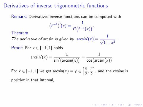
Derivatives of inverse trigonometric functions
Remark: Derivatives inverse functions can be computed with(f −1
)′(x) =
1
f ′(f −1(x)
) .
Theorem
The derivative of arcsin is given by arcsin′(x) =1√
1− x2.
Proof: For x ∈ [−1, 1] holds
arcsin′(x) =1
sin′(arcsin(x)
) =1
cos(arcsin(x)
)For x ∈ [−1, 1] we get arcsin(x) = y ∈
[π
2,π
2
], and the cosine is
positive in that interval, then cos(y) = +√
1− sin2(y), hence
arcsin′(x) =1√
1− sin2(arcsin(x)
) ⇒ arcsin′(x) =1√
1− x2.

Derivatives of inverse trigonometric functions
Remark: Derivatives inverse functions can be computed with(f −1
)′(x) =
1
f ′(f −1(x)
) .
Theorem
The derivative of arcsin is given by arcsin′(x) =1√
1− x2.
Proof: For x ∈ [−1, 1] holds
arcsin′(x) =1
sin′(arcsin(x)
)
=1
cos(arcsin(x)
)For x ∈ [−1, 1] we get arcsin(x) = y ∈
[π
2,π
2
], and the cosine is
positive in that interval, then cos(y) = +√
1− sin2(y), hence
arcsin′(x) =1√
1− sin2(arcsin(x)
) ⇒ arcsin′(x) =1√
1− x2.

Derivatives of inverse trigonometric functions
Remark: Derivatives inverse functions can be computed with(f −1
)′(x) =
1
f ′(f −1(x)
) .
Theorem
The derivative of arcsin is given by arcsin′(x) =1√
1− x2.
Proof: For x ∈ [−1, 1] holds
arcsin′(x) =1
sin′(arcsin(x)
) =1
cos(arcsin(x)
)
For x ∈ [−1, 1] we get arcsin(x) = y ∈[π
2,π
2
], and the cosine is
positive in that interval, then cos(y) = +√
1− sin2(y), hence
arcsin′(x) =1√
1− sin2(arcsin(x)
) ⇒ arcsin′(x) =1√
1− x2.

Derivatives of inverse trigonometric functions
Remark: Derivatives inverse functions can be computed with(f −1
)′(x) =
1
f ′(f −1(x)
) .
Theorem
The derivative of arcsin is given by arcsin′(x) =1√
1− x2.
Proof: For x ∈ [−1, 1] holds
arcsin′(x) =1
sin′(arcsin(x)
) =1
cos(arcsin(x)
)For x ∈ [−1, 1] we get arcsin(x) = y ∈
[π
2,π
2
],
and the cosine is
positive in that interval, then cos(y) = +√
1− sin2(y), hence
arcsin′(x) =1√
1− sin2(arcsin(x)
) ⇒ arcsin′(x) =1√
1− x2.
Derivatives of inverse trigonometric functions
Remark: Derivatives inverse functions can be computed with(f −1
)′(x) =
1
f ′(f −1(x)
) .
Theorem
The derivative of arcsin is given by arcsin′(x) =1√
1− x2.
Proof: For x ∈ [−1, 1] holds
arcsin′(x) =1
sin′(arcsin(x)
) =1
cos(arcsin(x)
)For x ∈ [−1, 1] we get arcsin(x) = y ∈
[π
2,π
2
], and the cosine is
positive in that interval,
then cos(y) = +√
1− sin2(y), hence
arcsin′(x) =1√
1− sin2(arcsin(x)
) ⇒ arcsin′(x) =1√
1− x2.

Derivatives of inverse trigonometric functions
Remark: Derivatives inverse functions can be computed with(f −1
)′(x) =
1
f ′(f −1(x)
) .
Theorem
The derivative of arcsin is given by arcsin′(x) =1√
1− x2.
Proof: For x ∈ [−1, 1] holds
arcsin′(x) =1
sin′(arcsin(x)
) =1
cos(arcsin(x)
)For x ∈ [−1, 1] we get arcsin(x) = y ∈
[π
2,π
2
], and the cosine is
positive in that interval, then cos(y) = +√
1− sin2(y),
hence
arcsin′(x) =1√
1− sin2(arcsin(x)
) ⇒ arcsin′(x) =1√
1− x2.

Derivatives of inverse trigonometric functions
Remark: Derivatives inverse functions can be computed with(f −1
)′(x) =
1
f ′(f −1(x)
) .
Theorem
The derivative of arcsin is given by arcsin′(x) =1√
1− x2.
Proof: For x ∈ [−1, 1] holds
arcsin′(x) =1
sin′(arcsin(x)
) =1
cos(arcsin(x)
)For x ∈ [−1, 1] we get arcsin(x) = y ∈
[π
2,π
2
], and the cosine is
positive in that interval, then cos(y) = +√
1− sin2(y), hence
arcsin′(x) =1√
1− sin2(arcsin(x)
)
⇒ arcsin′(x) =1√
1− x2.

Derivatives of inverse trigonometric functions
Remark: Derivatives inverse functions can be computed with(f −1
)′(x) =
1
f ′(f −1(x)
) .
Theorem
The derivative of arcsin is given by arcsin′(x) =1√
1− x2.
Proof: For x ∈ [−1, 1] holds
arcsin′(x) =1
sin′(arcsin(x)
) =1
cos(arcsin(x)
)For x ∈ [−1, 1] we get arcsin(x) = y ∈
[π
2,π
2
], and the cosine is
positive in that interval, then cos(y) = +√
1− sin2(y), hence
arcsin′(x) =1√
1− sin2(arcsin(x)
) ⇒ arcsin′(x) =1√
1− x2.

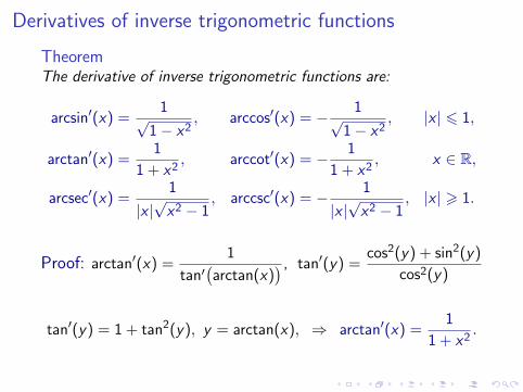
Derivatives of inverse trigonometric functions
TheoremThe derivative of inverse trigonometric functions are:
arcsin′(x) =1√
1− x2, arccos′(x) = − 1√
1− x2, |x | 6 1,
arctan′(x) =1
1 + x2, arccot′(x) = − 1
1 + x2, x ∈ R,
arcsec′(x) =1
|x |√
x2 − 1, arccsc′(x) = − 1
|x |√
x2 − 1, |x | > 1.
Proof: arctan′(x) =1
tan′(arctan(x)
) , tan′(y) =cos2(y) + sin2(y)
cos2(y)
tan′(y) = 1 + tan2(y), y = arctan(x), ⇒ arctan′(x) =1
1 + x2.

Derivatives of inverse trigonometric functions
TheoremThe derivative of inverse trigonometric functions are:
arcsin′(x) =1√
1− x2, arccos′(x) = − 1√
1− x2, |x | 6 1,
arctan′(x) =1
1 + x2, arccot′(x) = − 1
1 + x2, x ∈ R,
arcsec′(x) =1
|x |√
x2 − 1, arccsc′(x) = − 1
|x |√
x2 − 1, |x | > 1.
Proof: arctan′(x) =1
tan′(arctan(x)
) ,
tan′(y) =cos2(y) + sin2(y)
cos2(y)
tan′(y) = 1 + tan2(y), y = arctan(x), ⇒ arctan′(x) =1
1 + x2.

Derivatives of inverse trigonometric functions
TheoremThe derivative of inverse trigonometric functions are:
arcsin′(x) =1√
1− x2, arccos′(x) = − 1√
1− x2, |x | 6 1,
arctan′(x) =1
1 + x2, arccot′(x) = − 1
1 + x2, x ∈ R,
arcsec′(x) =1
|x |√
x2 − 1, arccsc′(x) = − 1
|x |√
x2 − 1, |x | > 1.
Proof: arctan′(x) =1
tan′(arctan(x)
) , tan′(y) =cos2(y) + sin2(y)
cos2(y)
tan′(y) = 1 + tan2(y), y = arctan(x), ⇒ arctan′(x) =1
1 + x2.

Derivatives of inverse trigonometric functions
TheoremThe derivative of inverse trigonometric functions are:
arcsin′(x) =1√
1− x2, arccos′(x) = − 1√
1− x2, |x | 6 1,
arctan′(x) =1
1 + x2, arccot′(x) = − 1
1 + x2, x ∈ R,
arcsec′(x) =1
|x |√
x2 − 1, arccsc′(x) = − 1
|x |√
x2 − 1, |x | > 1.
Proof: arctan′(x) =1
tan′(arctan(x)
) , tan′(y) =cos2(y) + sin2(y)
cos2(y)
tan′(y) = 1 + tan2(y),
y = arctan(x), ⇒ arctan′(x) =1
1 + x2.

Derivatives of inverse trigonometric functions
TheoremThe derivative of inverse trigonometric functions are:
arcsin′(x) =1√
1− x2, arccos′(x) = − 1√
1− x2, |x | 6 1,
arctan′(x) =1
1 + x2, arccot′(x) = − 1
1 + x2, x ∈ R,
arcsec′(x) =1
|x |√
x2 − 1, arccsc′(x) = − 1
|x |√
x2 − 1, |x | > 1.
Proof: arctan′(x) =1
tan′(arctan(x)
) , tan′(y) =cos2(y) + sin2(y)
cos2(y)
tan′(y) = 1 + tan2(y), y = arctan(x),
⇒ arctan′(x) =1
1 + x2.
Derivatives of inverse trigonometric functions
TheoremThe derivative of inverse trigonometric functions are:
arcsin′(x) =1√
1− x2, arccos′(x) = − 1√
1− x2, |x | 6 1,
arctan′(x) =1
1 + x2, arccot′(x) = − 1
1 + x2, x ∈ R,
arcsec′(x) =1
|x |√
x2 − 1, arccsc′(x) = − 1
|x |√
x2 − 1, |x | > 1.
Proof: arctan′(x) =1
tan′(arctan(x)
) , tan′(y) =cos2(y) + sin2(y)
cos2(y)
tan′(y) = 1 + tan2(y), y = arctan(x), ⇒ arctan′(x) =1
1 + x2.

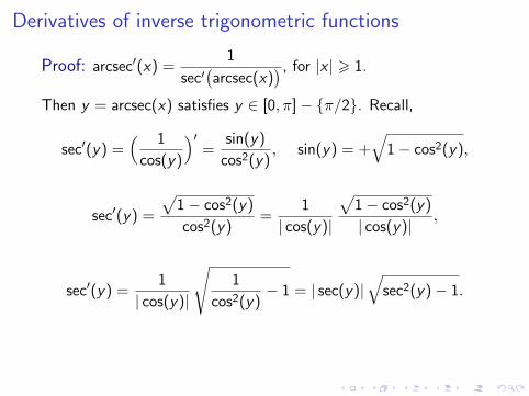
Derivatives of inverse trigonometric functions
Proof: arcsec′(x) =1
sec′(arcsec(x)
) ,
for |x | > 1.
Then y = arcsec(x) satisfies y ∈ [0, π]− {π/2}. Recall,
sec′(y) =( 1
cos(y)
)′=
sin(y)
cos2(y), sin(y) = +
√1− cos2(y),
sec′(y) =
√1− cos2(y)
cos2(y)=
1
| cos(y)|
√1− cos2(y)
| cos(y)|,
sec′(y) =1
| cos(y)|
√1
cos2(y)− 1 = | sec(y)|
√sec2(y)− 1.
We conclude: arcsec′(x) =1
|x |√
x2 − 1.

Derivatives of inverse trigonometric functions
Proof: arcsec′(x) =1
sec′(arcsec(x)
) , for |x | > 1.
Then y = arcsec(x) satisfies y ∈ [0, π]− {π/2}.
Recall,
sec′(y) =( 1
cos(y)
)′=
sin(y)
cos2(y), sin(y) = +
√1− cos2(y),
sec′(y) =
√1− cos2(y)
cos2(y)=
1
| cos(y)|
√1− cos2(y)
| cos(y)|,
sec′(y) =1
| cos(y)|
√1
cos2(y)− 1 = | sec(y)|
√sec2(y)− 1.
We conclude: arcsec′(x) =1
|x |√
x2 − 1.

Derivatives of inverse trigonometric functions
Proof: arcsec′(x) =1
sec′(arcsec(x)
) , for |x | > 1.
Then y = arcsec(x) satisfies y ∈ [0, π]− {π/2}. Recall,
sec′(y) =( 1
cos(y)
)′
=sin(y)
cos2(y), sin(y) = +
√1− cos2(y),
sec′(y) =
√1− cos2(y)
cos2(y)=
1
| cos(y)|
√1− cos2(y)
| cos(y)|,
sec′(y) =1
| cos(y)|
√1
cos2(y)− 1 = | sec(y)|
√sec2(y)− 1.
We conclude: arcsec′(x) =1
|x |√
x2 − 1.

Derivatives of inverse trigonometric functions
Proof: arcsec′(x) =1
sec′(arcsec(x)
) , for |x | > 1.
Then y = arcsec(x) satisfies y ∈ [0, π]− {π/2}. Recall,
sec′(y) =( 1
cos(y)
)′=
sin(y)
cos2(y),
sin(y) = +√
1− cos2(y),
sec′(y) =
√1− cos2(y)
cos2(y)=
1
| cos(y)|
√1− cos2(y)
| cos(y)|,
sec′(y) =1
| cos(y)|
√1
cos2(y)− 1 = | sec(y)|
√sec2(y)− 1.
We conclude: arcsec′(x) =1
|x |√
x2 − 1.

Derivatives of inverse trigonometric functions
Proof: arcsec′(x) =1
sec′(arcsec(x)
) , for |x | > 1.
Then y = arcsec(x) satisfies y ∈ [0, π]− {π/2}. Recall,
sec′(y) =( 1
cos(y)
)′=
sin(y)
cos2(y), sin(y) = +
√1− cos2(y),
sec′(y) =
√1− cos2(y)
cos2(y)=
1
| cos(y)|
√1− cos2(y)
| cos(y)|,
sec′(y) =1
| cos(y)|
√1
cos2(y)− 1 = | sec(y)|
√sec2(y)− 1.
We conclude: arcsec′(x) =1
|x |√
x2 − 1.

Derivatives of inverse trigonometric functions
Proof: arcsec′(x) =1
sec′(arcsec(x)
) , for |x | > 1.
Then y = arcsec(x) satisfies y ∈ [0, π]− {π/2}. Recall,
sec′(y) =( 1
cos(y)
)′=
sin(y)
cos2(y), sin(y) = +
√1− cos2(y),
sec′(y) =
√1− cos2(y)
cos2(y)
=1
| cos(y)|
√1− cos2(y)
| cos(y)|,
sec′(y) =1
| cos(y)|
√1
cos2(y)− 1 = | sec(y)|
√sec2(y)− 1.
We conclude: arcsec′(x) =1
|x |√
x2 − 1.

Derivatives of inverse trigonometric functions
Proof: arcsec′(x) =1
sec′(arcsec(x)
) , for |x | > 1.
Then y = arcsec(x) satisfies y ∈ [0, π]− {π/2}. Recall,
sec′(y) =( 1
cos(y)
)′=
sin(y)
cos2(y), sin(y) = +
√1− cos2(y),
sec′(y) =
√1− cos2(y)
cos2(y)=
1
| cos(y)|
√1− cos2(y)
| cos(y)|,
sec′(y) =1
| cos(y)|
√1
cos2(y)− 1 = | sec(y)|
√sec2(y)− 1.
We conclude: arcsec′(x) =1
|x |√
x2 − 1.

Derivatives of inverse trigonometric functions
Proof: arcsec′(x) =1
sec′(arcsec(x)
) , for |x | > 1.
Then y = arcsec(x) satisfies y ∈ [0, π]− {π/2}. Recall,
sec′(y) =( 1
cos(y)
)′=
sin(y)
cos2(y), sin(y) = +
√1− cos2(y),
sec′(y) =
√1− cos2(y)
cos2(y)=
1
| cos(y)|
√1− cos2(y)
| cos(y)|,
sec′(y) =1
| cos(y)|
√1
cos2(y)− 1
= | sec(y)|√
sec2(y)− 1.
We conclude: arcsec′(x) =1
|x |√
x2 − 1.
Derivatives of inverse trigonometric functions
Proof: arcsec′(x) =1
sec′(arcsec(x)
) , for |x | > 1.
Then y = arcsec(x) satisfies y ∈ [0, π]− {π/2}. Recall,
sec′(y) =( 1
cos(y)
)′=
sin(y)
cos2(y), sin(y) = +
√1− cos2(y),
sec′(y) =
√1− cos2(y)
cos2(y)=
1
| cos(y)|
√1− cos2(y)
| cos(y)|,
sec′(y) =1
| cos(y)|
√1
cos2(y)− 1 = | sec(y)|
√sec2(y)− 1.
We conclude: arcsec′(x) =1
|x |√
x2 − 1.

Derivatives of inverse trigonometric functions
Proof: arcsec′(x) =1
sec′(arcsec(x)
) , for |x | > 1.
Then y = arcsec(x) satisfies y ∈ [0, π]− {π/2}. Recall,
sec′(y) =( 1
cos(y)
)′=
sin(y)
cos2(y), sin(y) = +
√1− cos2(y),
sec′(y) =
√1− cos2(y)
cos2(y)=
1
| cos(y)|
√1− cos2(y)
| cos(y)|,
sec′(y) =1
| cos(y)|
√1
cos2(y)− 1 = | sec(y)|
√sec2(y)− 1.
We conclude: arcsec′(x) =1
|x |√
x2 − 1.

Derivatives of inverse trigonometric functions
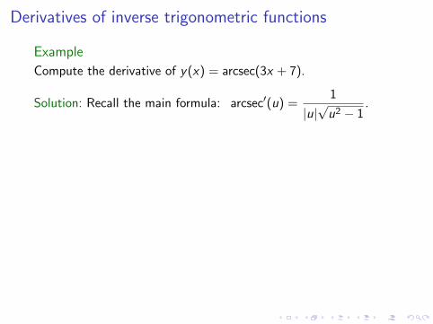
Example
Compute the derivative of y(x) = arcsec(3x + 7).
Solution: Recall the main formula: arcsec′(u) =1
|u|√
u2 − 1.
Then, chain rule implies, y ′(x) =3
|3x + 7|√
(3x + 7)2 − 1. C
Example
Compute the derivative of y(x) = arctan(4 ln(x)).
Solution: Recall the main formula: arctan′(u) =1
1 + u2.
Therefore, chain rule implies,
y ′(x) =1[
1 +(4 ln(x)
)2] 4
x⇒ y ′ =
4
x[1 + 16 ln2(x)
] . C
Derivatives of inverse trigonometric functions
Example
Compute the derivative of y(x) = arcsec(3x + 7).
Solution: Recall the main formula: arcsec′(u) =1
|u|√
u2 − 1.
Then, chain rule implies, y ′(x) =3
|3x + 7|√
(3x + 7)2 − 1. C
Example
Compute the derivative of y(x) = arctan(4 ln(x)).
Solution: Recall the main formula: arctan′(u) =1
1 + u2.
Therefore, chain rule implies,
y ′(x) =1[
1 +(4 ln(x)
)2] 4
x⇒ y ′ =
4
x[1 + 16 ln2(x)
] . C

Derivatives of inverse trigonometric functions
Example
Compute the derivative of y(x) = arcsec(3x + 7).
Solution: Recall the main formula: arcsec′(u) =1
|u|√
u2 − 1.
Then, chain rule implies,
y ′(x) =3
|3x + 7|√
(3x + 7)2 − 1. C
Example
Compute the derivative of y(x) = arctan(4 ln(x)).
Solution: Recall the main formula: arctan′(u) =1
1 + u2.
Therefore, chain rule implies,
y ′(x) =1[
1 +(4 ln(x)
)2] 4
x⇒ y ′ =
4
x[1 + 16 ln2(x)
] . C

Derivatives of inverse trigonometric functions
Example
Compute the derivative of y(x) = arcsec(3x + 7).
Solution: Recall the main formula: arcsec′(u) =1
|u|√
u2 − 1.
Then, chain rule implies, y ′(x) =3
|3x + 7|√
(3x + 7)2 − 1. C
Example
Compute the derivative of y(x) = arctan(4 ln(x)).
Solution: Recall the main formula: arctan′(u) =1
1 + u2.
Therefore, chain rule implies,
y ′(x) =1[
1 +(4 ln(x)
)2] 4
x⇒ y ′ =
4
x[1 + 16 ln2(x)
] . C

Derivatives of inverse trigonometric functions
Example
Compute the derivative of y(x) = arcsec(3x + 7).
Solution: Recall the main formula: arcsec′(u) =1
|u|√
u2 − 1.
Then, chain rule implies, y ′(x) =3
|3x + 7|√
(3x + 7)2 − 1. C
Example
Compute the derivative of y(x) = arctan(4 ln(x)).
Solution: Recall the main formula: arctan′(u) =1
1 + u2.
Therefore, chain rule implies,
y ′(x) =1[
1 +(4 ln(x)
)2] 4
x
⇒ y ′ =4
x[1 + 16 ln2(x)
] . C

Derivatives of inverse trigonometric functions
Example
Compute the derivative of y(x) = arcsec(3x + 7).
Solution: Recall the main formula: arcsec′(u) =1
|u|√
u2 − 1.
Then, chain rule implies, y ′(x) =3
|3x + 7|√
(3x + 7)2 − 1. C
Example
Compute the derivative of y(x) = arctan(4 ln(x)).
Solution: Recall the main formula: arctan′(u) =1
1 + u2.
Therefore, chain rule implies,
y ′(x) =1[
1 +(4 ln(x)
)2] 4
x⇒ y ′ =
4
x[1 + 16 ln2(x)
] . C

Inverse trigonometric functions (Sect. 7.6)
Today: Derivatives and integrals.
I Review: Definitions and properties.
I Derivatives.
I Integrals.

Integrals of inverse trigonometric functions
Remark: The formulas for the derivatives of inverse trigonometricfunctions imply the integration formulas.
TheoremFor any constant a 6= 0 holds,∫
dx√a2 − x2
= arcsin(x
a
)+ c , |x | < a,∫
dx
a2 + x2=
1
aarctan
(x
a
)+ c , x ∈ R,∫
dx
x√
x2 − a2=
1
aarcsec
(∣∣∣xa
∣∣∣) + c , |x | > a > 0.
Proof: (For arcsine only.) y(x) = arcsin(x
a
)+ c , then
y ′(x) =1√
1− x2
a2
1
a=
|a|√a2 − x2
1
a⇒ y ′(x) =
1√a2 − x2

Integrals of inverse trigonometric functions
Remark: The formulas for the derivatives of inverse trigonometricfunctions imply the integration formulas.
TheoremFor any constant a 6= 0 holds,∫
dx√a2 − x2
= arcsin(x
a
)+ c , |x | < a,∫
dx
a2 + x2=
1
aarctan
(x
a
)+ c , x ∈ R,∫
dx
x√
x2 − a2=
1
aarcsec
(∣∣∣xa
∣∣∣) + c , |x | > a > 0.
Proof: (For arcsine only.)
y(x) = arcsin(x
a
)+ c , then
y ′(x) =1√
1− x2
a2
1
a=
|a|√a2 − x2
1
a⇒ y ′(x) =
1√a2 − x2

Integrals of inverse trigonometric functions
Remark: The formulas for the derivatives of inverse trigonometricfunctions imply the integration formulas.
TheoremFor any constant a 6= 0 holds,∫
dx√a2 − x2
= arcsin(x
a
)+ c , |x | < a,∫
dx
a2 + x2=
1
aarctan
(x
a
)+ c , x ∈ R,∫
dx
x√
x2 − a2=
1
aarcsec
(∣∣∣xa
∣∣∣) + c , |x | > a > 0.
Proof: (For arcsine only.) y(x) = arcsin(x
a
)+ c ,
then
y ′(x) =1√
1− x2
a2
1
a=
|a|√a2 − x2
1
a⇒ y ′(x) =
1√a2 − x2

Integrals of inverse trigonometric functions
Remark: The formulas for the derivatives of inverse trigonometricfunctions imply the integration formulas.
TheoremFor any constant a 6= 0 holds,∫
dx√a2 − x2
= arcsin(x
a
)+ c , |x | < a,∫
dx
a2 + x2=
1
aarctan
(x
a
)+ c , x ∈ R,∫
dx
x√
x2 − a2=
1
aarcsec
(∣∣∣xa
∣∣∣) + c , |x | > a > 0.
Proof: (For arcsine only.) y(x) = arcsin(x
a
)+ c , then
y ′(x)
=1√
1− x2
a2
1
a=
|a|√a2 − x2
1
a⇒ y ′(x) =
1√a2 − x2

Integrals of inverse trigonometric functions
Remark: The formulas for the derivatives of inverse trigonometricfunctions imply the integration formulas.
TheoremFor any constant a 6= 0 holds,∫
dx√a2 − x2
= arcsin(x
a
)+ c , |x | < a,∫
dx
a2 + x2=
1
aarctan
(x
a
)+ c , x ∈ R,∫
dx
x√
x2 − a2=
1
aarcsec
(∣∣∣xa
∣∣∣) + c , |x | > a > 0.
Proof: (For arcsine only.) y(x) = arcsin(x
a
)+ c , then
y ′(x) =1√
1− x2
a2
1
a
=|a|√
a2 − x2
1
a⇒ y ′(x) =
1√a2 − x2

Integrals of inverse trigonometric functions
Remark: The formulas for the derivatives of inverse trigonometricfunctions imply the integration formulas.
TheoremFor any constant a 6= 0 holds,∫
dx√a2 − x2
= arcsin(x
a
)+ c , |x | < a,∫
dx
a2 + x2=
1
aarctan
(x
a
)+ c , x ∈ R,∫
dx
x√
x2 − a2=
1
aarcsec
(∣∣∣xa
∣∣∣) + c , |x | > a > 0.
Proof: (For arcsine only.) y(x) = arcsin(x
a
)+ c , then
y ′(x) =1√
1− x2
a2
1
a=
|a|√a2 − x2
1
a
⇒ y ′(x) =1√
a2 − x2

Integrals of inverse trigonometric functions
Remark: The formulas for the derivatives of inverse trigonometricfunctions imply the integration formulas.
TheoremFor any constant a 6= 0 holds,∫
dx√a2 − x2
= arcsin(x
a
)+ c , |x | < a,∫
dx
a2 + x2=
1
aarctan
(x
a
)+ c , x ∈ R,∫
dx
x√
x2 − a2=
1
aarcsec
(∣∣∣xa
∣∣∣) + c , |x | > a > 0.
Proof: (For arcsine only.) y(x) = arcsin(x
a
)+ c , then
y ′(x) =1√
1− x2
a2
1
a=
|a|√a2 − x2
1
a⇒ y ′(x) =
1√a2 − x2

Integrals of inverse trigonometric functions
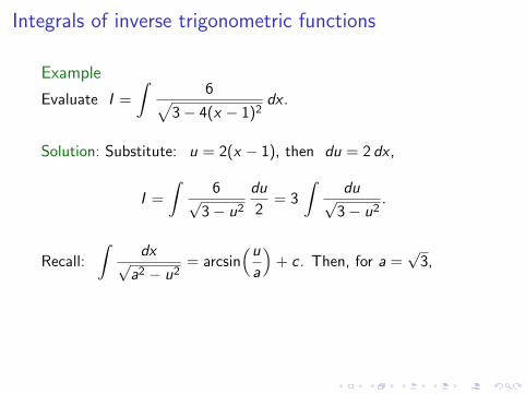
Example
Evaluate I =
∫6√
3− 4(x − 1)2dx .
Solution: Substitute: u = 2(x − 1), then du = 2 dx ,
I =
∫6√
3− u2
du
2= 3
∫du√
3− u2.
Recall:
∫dx√
a2 − u2= arcsin
(u
a
)+ c . Then, for a =
√3,
I = 3 arcsin( u√
3
)+ c ⇒ I = 3 arcsin
(2(x − 1)√3
)+ c . C

Integrals of inverse trigonometric functions
Example
Evaluate I =
∫6√
3− 4(x − 1)2dx .
Solution: Substitute: u = 2(x − 1),
then du = 2 dx ,
I =
∫6√
3− u2
du
2= 3
∫du√
3− u2.
Recall:
∫dx√
a2 − u2= arcsin
(u
a
)+ c . Then, for a =
√3,
I = 3 arcsin( u√
3
)+ c ⇒ I = 3 arcsin
(2(x − 1)√3
)+ c . C

Integrals of inverse trigonometric functions
Example
Evaluate I =
∫6√
3− 4(x − 1)2dx .
Solution: Substitute: u = 2(x − 1), then du = 2 dx ,
I =
∫6√
3− u2
du
2= 3
∫du√
3− u2.
Recall:
∫dx√
a2 − u2= arcsin
(u
a
)+ c . Then, for a =
√3,
I = 3 arcsin( u√
3
)+ c ⇒ I = 3 arcsin
(2(x − 1)√3
)+ c . C

Integrals of inverse trigonometric functions
Example
Evaluate I =
∫6√
3− 4(x − 1)2dx .
Solution: Substitute: u = 2(x − 1), then du = 2 dx ,
I =
∫6√
3− u2
du
2
= 3
∫du√
3− u2.
Recall:
∫dx√
a2 − u2= arcsin
(u
a
)+ c . Then, for a =
√3,
I = 3 arcsin( u√
3
)+ c ⇒ I = 3 arcsin
(2(x − 1)√3
)+ c . C

Integrals of inverse trigonometric functions
Example
Evaluate I =
∫6√
3− 4(x − 1)2dx .
Solution: Substitute: u = 2(x − 1), then du = 2 dx ,
I =
∫6√
3− u2
du
2= 3
∫du√
3− u2.
Recall:
∫dx√
a2 − u2= arcsin
(u
a
)+ c . Then, for a =
√3,
I = 3 arcsin( u√
3
)+ c ⇒ I = 3 arcsin
(2(x − 1)√3
)+ c . C

Integrals of inverse trigonometric functions
Example
Evaluate I =
∫6√
3− 4(x − 1)2dx .
Solution: Substitute: u = 2(x − 1), then du = 2 dx ,
I =
∫6√
3− u2
du
2= 3
∫du√
3− u2.
Recall:
∫dx√
a2 − u2= arcsin
(u
a
)+ c .
Then, for a =√
3,
I = 3 arcsin( u√
3
)+ c ⇒ I = 3 arcsin
(2(x − 1)√3
)+ c . C
Integrals of inverse trigonometric functions
Example
Evaluate I =
∫6√
3− 4(x − 1)2dx .
Solution: Substitute: u = 2(x − 1), then du = 2 dx ,
I =
∫6√
3− u2
du
2= 3
∫du√
3− u2.
Recall:
∫dx√
a2 − u2= arcsin
(u
a
)+ c . Then, for a =
√3,
I = 3 arcsin( u√
3
)+ c ⇒ I = 3 arcsin
(2(x − 1)√3
)+ c . C

Integrals of inverse trigonometric functions
Example
Evaluate I =
∫6√
3− 4(x − 1)2dx .
Solution: Substitute: u = 2(x − 1), then du = 2 dx ,
I =
∫6√
3− u2
du
2= 3
∫du√
3− u2.
Recall:
∫dx√
a2 − u2= arcsin
(u
a
)+ c . Then, for a =
√3,
I = 3 arcsin( u√
3
)+ c
⇒ I = 3 arcsin(2(x − 1)√
3
)+ c . C

Integrals of inverse trigonometric functions
Example
Evaluate I =
∫6√
3− 4(x − 1)2dx .
Solution: Substitute: u = 2(x − 1), then du = 2 dx ,
I =
∫6√
3− u2
du
2= 3
∫du√
3− u2.
Recall:
∫dx√
a2 − u2= arcsin
(u
a
)+ c . Then, for a =
√3,
I = 3 arcsin( u√
3
)+ c ⇒ I = 3 arcsin
(2(x − 1)√3
)+ c . C

Integrals of inverse trigonometric functions
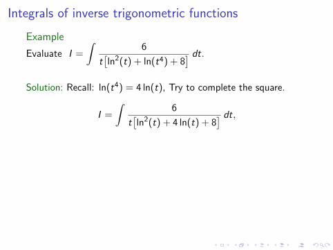
Example
Evaluate I =
∫6
t[ln2(t) + ln(t4) + 8
] dt.
Solution: Recall: ln(t4) = 4 ln(t), Try to complete the square.
I =
∫6
t[ln2(t) + 4 ln(t) + 8
] dt,
I =
∫6
t[ln2(t) + 2(2 ln(t)) + 4− 4 + 8
] dt
I =
∫6
t[(
ln(t) + 2)2
+ 4] dt
This looks like the derivative of the arctangent.

Integrals of inverse trigonometric functions
Example
Evaluate I =
∫6
t[ln2(t) + ln(t4) + 8
] dt.
Solution: Recall: ln(t4) = 4 ln(t),
Try to complete the square.
I =
∫6
t[ln2(t) + 4 ln(t) + 8
] dt,
I =
∫6
t[ln2(t) + 2(2 ln(t)) + 4− 4 + 8
] dt
I =
∫6
t[(
ln(t) + 2)2
+ 4] dt
This looks like the derivative of the arctangent.

Integrals of inverse trigonometric functions
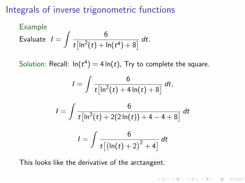
Example
Evaluate I =
∫6
t[ln2(t) + ln(t4) + 8
] dt.
Solution: Recall: ln(t4) = 4 ln(t), Try to complete the square.
I =
∫6
t[ln2(t) + 4 ln(t) + 8
] dt,
I =
∫6
t[ln2(t) + 2(2 ln(t)) + 4− 4 + 8
] dt
I =
∫6
t[(
ln(t) + 2)2
+ 4] dt
This looks like the derivative of the arctangent.
Integrals of inverse trigonometric functions
Example
Evaluate I =
∫6
t[ln2(t) + ln(t4) + 8
] dt.
Solution: Recall: ln(t4) = 4 ln(t), Try to complete the square.
I =
∫6
t[ln2(t) + 4 ln(t) + 8
] dt,
I =
∫6
t[ln2(t) + 2(2 ln(t)) + 4− 4 + 8
] dt
I =
∫6
t[(
ln(t) + 2)2
+ 4] dt
This looks like the derivative of the arctangent.
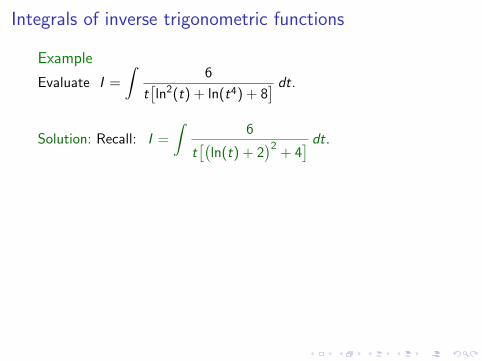
Integrals of inverse trigonometric functions
Example
Evaluate I =
∫6
t[ln2(t) + ln(t4) + 8
] dt.
Solution: Recall: I =
∫6
t[(
ln(t) + 2)2
+ 4] dt.
Substitute: u = ln(t) + 2, then du =1
tdt,
I =
∫6
4 + u2du = 6
∫du
22 + u2= 6
1
2arctan
(u
2
)+ c .
I = 3 arctan(1
2(ln(t)+2)
)+c ⇒ I = 3 arctan
(ln(√
t)+1)+c .C

Integrals of inverse trigonometric functions
Example
Evaluate I =
∫6
t[ln2(t) + ln(t4) + 8
] dt.
Solution: Recall: I =
∫6
t[(
ln(t) + 2)2
+ 4] dt.
Substitute: u = ln(t) + 2,
then du =1
tdt,
I =
∫6
4 + u2du = 6
∫du
22 + u2= 6
1
2arctan
(u
2
)+ c .
I = 3 arctan(1
2(ln(t)+2)
)+c ⇒ I = 3 arctan
(ln(√
t)+1)+c .C

Integrals of inverse trigonometric functions
Example
Evaluate I =
∫6
t[ln2(t) + ln(t4) + 8
] dt.
Solution: Recall: I =
∫6
t[(
ln(t) + 2)2
+ 4] dt.
Substitute: u = ln(t) + 2, then du =1
tdt,
I =
∫6
4 + u2du = 6
∫du
22 + u2= 6
1
2arctan
(u
2
)+ c .
I = 3 arctan(1
2(ln(t)+2)
)+c ⇒ I = 3 arctan
(ln(√
t)+1)+c .C

Integrals of inverse trigonometric functions
Example
Evaluate I =
∫6
t[ln2(t) + ln(t4) + 8
] dt.
Solution: Recall: I =
∫6
t[(
ln(t) + 2)2
+ 4] dt.
Substitute: u = ln(t) + 2, then du =1
tdt,
I =
∫6
4 + u2du
= 6
∫du
22 + u2= 6
1
2arctan
(u
2
)+ c .
I = 3 arctan(1
2(ln(t)+2)
)+c ⇒ I = 3 arctan
(ln(√
t)+1)+c .C

Integrals of inverse trigonometric functions
Example
Evaluate I =
∫6
t[ln2(t) + ln(t4) + 8
] dt.
Solution: Recall: I =
∫6
t[(
ln(t) + 2)2
+ 4] dt.
Substitute: u = ln(t) + 2, then du =1
tdt,
I =
∫6
4 + u2du = 6
∫du
22 + u2
= 61
2arctan
(u
2
)+ c .
I = 3 arctan(1
2(ln(t)+2)
)+c ⇒ I = 3 arctan
(ln(√
t)+1)+c .C

Integrals of inverse trigonometric functions
Example
Evaluate I =
∫6
t[ln2(t) + ln(t4) + 8
] dt.
Solution: Recall: I =
∫6
t[(
ln(t) + 2)2
+ 4] dt.
Substitute: u = ln(t) + 2, then du =1
tdt,
I =
∫6
4 + u2du = 6
∫du
22 + u2= 6
1
2arctan
(u
2
)+ c .
I = 3 arctan(1
2(ln(t)+2)
)+c ⇒ I = 3 arctan
(ln(√
t)+1)+c .C

Integrals of inverse trigonometric functions
Example
Evaluate I =
∫6
t[ln2(t) + ln(t4) + 8
] dt.
Solution: Recall: I =
∫6
t[(
ln(t) + 2)2
+ 4] dt.
Substitute: u = ln(t) + 2, then du =1
tdt,
I =
∫6
4 + u2du = 6
∫du
22 + u2= 6
1
2arctan
(u
2
)+ c .
I = 3 arctan(1
2(ln(t)+2)
)+c
⇒ I = 3 arctan(ln(√
t)+1)+c .C

Integrals of inverse trigonometric functions
Example
Evaluate I =
∫6
t[ln2(t) + ln(t4) + 8
] dt.
Solution: Recall: I =
∫6
t[(
ln(t) + 2)2
+ 4] dt.
Substitute: u = ln(t) + 2, then du =1
tdt,
I =
∫6
4 + u2du = 6
∫du
22 + u2= 6
1
2arctan
(u
2
)+ c .
I = 3 arctan(1
2(ln(t)+2)
)+c ⇒ I = 3 arctan
(ln(√
t)+1)+c .C

Hyperbolic functions (Sect. 7.7)
I Circular and hyperbolic functions.
I Definitions and identities.
I Derivatives of hyperbolic functions.
I Integrals of hyperbolic functions.

Circular and hyperbolic functions
Remark: Trigonometric functions are also called circular functions.
(θ)
y
x1
θ
cos (θ)
sin
The circle x2 + y2 = 1 can beparametrized by the functions
x = cos(θ),
y = sin(θ).
Since these functions satisfy
cos2(θ) + sin2(θ) = 1.
Remark: The parametrization is not unique. Another solution is
x = cos(nθ), y = sin(nθ), n ∈ N.

Circular and hyperbolic functions
Remark: Trigonometric functions are also called circular functions.
(θ)
y
x1
θ
cos (θ)
sin
The circle x2 + y2 = 1 can beparametrized by the functions
x = cos(θ),
y = sin(θ).
Since these functions satisfy
cos2(θ) + sin2(θ) = 1.
Remark: The parametrization is not unique.
Another solution is
x = cos(nθ), y = sin(nθ), n ∈ N.

Circular and hyperbolic functions
Remark: Trigonometric functions are also called circular functions.
(θ)
y
x1
θ
cos (θ)
sin
The circle x2 + y2 = 1 can beparametrized by the functions
x = cos(θ),
y = sin(θ).
Since these functions satisfy
cos2(θ) + sin2(θ) = 1.
Remark: The parametrization is not unique. Another solution is
x = cos(nθ), y = sin(nθ), n ∈ N.

Circular and hyperbolic functions
Remark:Hyperbolic functions are a parametrization of a hyperbola.
y(u)
y
x1
x(u)
The hyperbola x2 − y2 = 1 canbe parametrized by the functions
x = f (u), y = g(u),
satisfying the condition
f 2(u)− g2(u) = 1.
Remark: A solution is x =1
2
[h(u) +
1
h(u)
], y =
1
2
[h(u)− 1
h(u)
],
x2 − y2 =1
4
[h2 +
1
h2+ 2− h2 − 1
h2+ 2
]= 1.

Circular and hyperbolic functions
Remark:Hyperbolic functions are a parametrization of a hyperbola.
y(u)
y
x1
x(u)
The hyperbola x2 − y2 = 1 canbe parametrized by the functions
x = f (u), y = g(u),
satisfying the condition
f 2(u)− g2(u) = 1.
Remark: A solution is x =1
2
[h(u) +
1
h(u)
], y =
1
2
[h(u)− 1
h(u)
],
x2 − y2 =
1
4
[h2 +
1
h2+ 2− h2 − 1
h2+ 2
]= 1.

Circular and hyperbolic functions
Remark:Hyperbolic functions are a parametrization of a hyperbola.
y(u)
y
x1
x(u)
The hyperbola x2 − y2 = 1 canbe parametrized by the functions
x = f (u), y = g(u),
satisfying the condition
f 2(u)− g2(u) = 1.
Remark: A solution is x =1
2
[h(u) +
1
h(u)
], y =
1
2
[h(u)− 1
h(u)
],
x2 − y2 =1
4
[h2 +
1
h2+ 2
− h2 − 1
h2+ 2
]= 1.

Circular and hyperbolic functions
Remark:Hyperbolic functions are a parametrization of a hyperbola.
y(u)
y
x1
x(u)
The hyperbola x2 − y2 = 1 canbe parametrized by the functions
x = f (u), y = g(u),
satisfying the condition
f 2(u)− g2(u) = 1.
Remark: A solution is x =1
2
[h(u) +
1
h(u)
], y =
1
2
[h(u)− 1
h(u)
],
x2 − y2 =1
4
[h2 +
1
h2+ 2− h2 − 1
h2+ 2
]
= 1.

Circular and hyperbolic functions
Remark:Hyperbolic functions are a parametrization of a hyperbola.
y(u)
y
x1
x(u)
The hyperbola x2 − y2 = 1 canbe parametrized by the functions
x = f (u), y = g(u),
satisfying the condition
f 2(u)− g2(u) = 1.
Remark: A solution is x =1
2
[h(u) +
1
h(u)
], y =
1
2
[h(u)− 1
h(u)
],
x2 − y2 =1
4
[h2 +
1
h2+ 2− h2 − 1
h2+ 2
]= 1.

Circular and hyperbolic functions
Remarks:
I The hyperbola x2 − y2 = 1 can be parametrized by
x =1
2
[h(u) +
1
h(u)
], y =
1
2
[h(u)− 1
h(u)
],
where h is any non-zero continuous function satisfying
limu→∞
h(u) = ∞, limu→−∞
h(u) = 0, h(0) = 1.
I The hyperbolic trigonometric functions correspond to
h(u) = eu.
DefinitionThe hyperbolic trigonometric functions are defined by
cosh(u) =eu + e−u
2, sinh(u) =
eu − e−u
2.

Circular and hyperbolic functions
Remarks:
I The hyperbola x2 − y2 = 1 can be parametrized by
x =1
2
[h(u) +
1
h(u)
], y =
1
2
[h(u)− 1
h(u)
],
where h is any non-zero continuous function satisfying
limu→∞
h(u) = ∞,
limu→−∞
h(u) = 0, h(0) = 1.
I The hyperbolic trigonometric functions correspond to
h(u) = eu.
DefinitionThe hyperbolic trigonometric functions are defined by
cosh(u) =eu + e−u
2, sinh(u) =
eu − e−u
2.

Circular and hyperbolic functions
Remarks:
I The hyperbola x2 − y2 = 1 can be parametrized by
x =1
2
[h(u) +
1
h(u)
], y =
1
2
[h(u)− 1
h(u)
],
where h is any non-zero continuous function satisfying
limu→∞
h(u) = ∞, limu→−∞
h(u) = 0,
h(0) = 1.
I The hyperbolic trigonometric functions correspond to
h(u) = eu.
DefinitionThe hyperbolic trigonometric functions are defined by
cosh(u) =eu + e−u
2, sinh(u) =
eu − e−u
2.

Circular and hyperbolic functions
Remarks:
I The hyperbola x2 − y2 = 1 can be parametrized by
x =1
2
[h(u) +
1
h(u)
], y =
1
2
[h(u)− 1
h(u)
],
where h is any non-zero continuous function satisfying
limu→∞
h(u) = ∞, limu→−∞
h(u) = 0, h(0) = 1.
I The hyperbolic trigonometric functions correspond to
h(u) = eu.
DefinitionThe hyperbolic trigonometric functions are defined by
cosh(u) =eu + e−u
2, sinh(u) =
eu − e−u
2.

Circular and hyperbolic functions
Remarks:
I The hyperbola x2 − y2 = 1 can be parametrized by
x =1
2
[h(u) +
1
h(u)
], y =
1
2
[h(u)− 1
h(u)
],
where h is any non-zero continuous function satisfying
limu→∞
h(u) = ∞, limu→−∞
h(u) = 0, h(0) = 1.
I The hyperbolic trigonometric functions correspond to
h(u) = eu.
DefinitionThe hyperbolic trigonometric functions are defined by
cosh(u) =eu + e−u
2, sinh(u) =
eu − e−u
2.

Hyperbolic functions (Sect. 7.7)
I Circular and hyperbolic functions.
I Definitions and identities.
I Derivatives of hyperbolic functions.
I Integrals of hyperbolic functions.

Definitions and identities
DefinitionThe complete set of hyperbolic trigonometric functions is given by
cosh(x) =ex + e−x
2, sinh(x) =
ex − e−x
2,
tanh(x) =sinh(x)
cosh(x), coth(x) =
cosh(x)
sinh(x),
csch(x) =1
sinh(x), sech(x) =
1
cosh(x).
Remarks:
I These functions satisfy identities similar but not equal tothose satisfied by circular trigonometric functions.
I We have seen one of these identities:
cosh2(x)− sinh2(x) = 1.

Definitions and identities
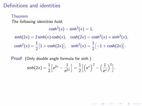
TheoremThe following identities hold,
cosh2(x)− sinh2(x) = 1,
sinh(2x) = 2 sinh(x) cosh(x), cosh(2x) = cosh2(x) + sinh2(x),
cosh2(x) =1
2
[1 + cosh(2x)
], sinh2(x) =
1
2
[−1 + cosh(2x)
].
Proof: (Only double angle formula for sinh.)
sinh(2x) =1
2
[e2x − 1
e2x
]=
1
2
[(ex
)2−
( 1
ex
)2].
Recalling the formula a2 − b2 = (a + b)(a− b),
sinh(2x) =2
4
[ex +
1
ex
][ex − 1
ex
]= 2 cosh(x) sinh(x).

Definitions and identities
TheoremThe following identities hold,
cosh2(x)− sinh2(x) = 1,
sinh(2x) = 2 sinh(x) cosh(x), cosh(2x) = cosh2(x) + sinh2(x),
cosh2(x) =1
2
[1 + cosh(2x)
], sinh2(x) =
1
2
[−1 + cosh(2x)
].
Proof: (Only double angle formula for sinh.)
sinh(2x) =1
2
[e2x − 1
e2x
]
=1
2
[(ex
)2−
( 1
ex
)2].
Recalling the formula a2 − b2 = (a + b)(a− b),
sinh(2x) =2
4
[ex +
1
ex
][ex − 1
ex
]= 2 cosh(x) sinh(x).
Definitions and identities
TheoremThe following identities hold,
cosh2(x)− sinh2(x) = 1,
sinh(2x) = 2 sinh(x) cosh(x), cosh(2x) = cosh2(x) + sinh2(x),
cosh2(x) =1
2
[1 + cosh(2x)
], sinh2(x) =
1
2
[−1 + cosh(2x)
].
Proof: (Only double angle formula for sinh.)
sinh(2x) =1
2
[e2x − 1
e2x
]=
1
2
[(ex
)2−
( 1
ex
)2].
Recalling the formula a2 − b2 = (a + b)(a− b),
sinh(2x) =2
4
[ex +
1
ex
][ex − 1
ex
]= 2 cosh(x) sinh(x).

Definitions and identities
TheoremThe following identities hold,
cosh2(x)− sinh2(x) = 1,
sinh(2x) = 2 sinh(x) cosh(x), cosh(2x) = cosh2(x) + sinh2(x),
cosh2(x) =1
2
[1 + cosh(2x)
], sinh2(x) =
1
2
[−1 + cosh(2x)
].
Proof: (Only double angle formula for sinh.)
sinh(2x) =1
2
[e2x − 1
e2x
]=
1
2
[(ex
)2−
( 1
ex
)2].
Recalling the formula a2 − b2 = (a + b)(a− b),
sinh(2x) =2
4
[ex +
1
ex
][ex − 1
ex
]
= 2 cosh(x) sinh(x).

Definitions and identities
TheoremThe following identities hold,
cosh2(x)− sinh2(x) = 1,
sinh(2x) = 2 sinh(x) cosh(x), cosh(2x) = cosh2(x) + sinh2(x),
cosh2(x) =1
2
[1 + cosh(2x)
], sinh2(x) =
1
2
[−1 + cosh(2x)
].
Proof: (Only double angle formula for sinh.)
sinh(2x) =1
2
[e2x − 1
e2x
]=
1
2
[(ex
)2−
( 1
ex
)2].
Recalling the formula a2 − b2 = (a + b)(a− b),
sinh(2x) =2
4
[ex +
1
ex
][ex − 1
ex
]= 2 cosh(x) sinh(x).

Definitions and identities
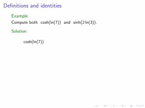
Example
Compute both cosh(ln(7)) and sinh(2 ln(3)).
Solution:
cosh(ln(7)) =1
2
[e ln(7) +
1
e ln(7)
]=
1
2
[7 +
1
7
]=
1
2
50
7.
We conclude that cosh(ln(7)) =25
7.
sinh(2 ln(3)) =1
2
[e2 ln(3) − 1
e2 ln(3)
]=
1
2
[e ln(9) − 1
e ln(9)
]
sinh(2 ln(3)) =1
2
[9− 1
9
]=
1
2
80
9⇒ sinh(2 ln(3)) =
40
9.C
Definitions and identities
Example
Compute both cosh(ln(7)) and sinh(2 ln(3)).
Solution:
cosh(ln(7))
=1
2
[e ln(7) +
1
e ln(7)
]=
1
2
[7 +
1
7
]=
1
2
50
7.
We conclude that cosh(ln(7)) =25
7.
sinh(2 ln(3)) =1
2
[e2 ln(3) − 1
e2 ln(3)
]=
1
2
[e ln(9) − 1
e ln(9)
]
sinh(2 ln(3)) =1
2
[9− 1
9
]=
1
2
80
9⇒ sinh(2 ln(3)) =
40
9.C

Definitions and identities
Example
Compute both cosh(ln(7)) and sinh(2 ln(3)).
Solution:
cosh(ln(7)) =1
2
[e ln(7) +
1
e ln(7)
]
=1
2
[7 +
1
7
]=
1
2
50
7.
We conclude that cosh(ln(7)) =25
7.
sinh(2 ln(3)) =1
2
[e2 ln(3) − 1
e2 ln(3)
]=
1
2
[e ln(9) − 1
e ln(9)
]
sinh(2 ln(3)) =1
2
[9− 1
9
]=
1
2
80
9⇒ sinh(2 ln(3)) =
40
9.C

Definitions and identities
Example
Compute both cosh(ln(7)) and sinh(2 ln(3)).
Solution:
cosh(ln(7)) =1
2
[e ln(7) +
1
e ln(7)
]=
1
2
[7 +
1
7
]
=1
2
50
7.
We conclude that cosh(ln(7)) =25
7.
sinh(2 ln(3)) =1
2
[e2 ln(3) − 1
e2 ln(3)
]=
1
2
[e ln(9) − 1
e ln(9)
]
sinh(2 ln(3)) =1
2
[9− 1
9
]=
1
2
80
9⇒ sinh(2 ln(3)) =
40
9.C

Definitions and identities
Example
Compute both cosh(ln(7)) and sinh(2 ln(3)).
Solution:
cosh(ln(7)) =1
2
[e ln(7) +
1
e ln(7)
]=
1
2
[7 +
1
7
]=
1
2
50
7.
We conclude that cosh(ln(7)) =25
7.
sinh(2 ln(3))
=1
2
[e2 ln(3) − 1
e2 ln(3)
]=
1
2
[e ln(9) − 1
e ln(9)
]
sinh(2 ln(3)) =1
2
[9− 1
9
]=
1
2
80
9⇒ sinh(2 ln(3)) =
40
9.C

Definitions and identities
Example
Compute both cosh(ln(7)) and sinh(2 ln(3)).
Solution:
cosh(ln(7)) =1
2
[e ln(7) +
1
e ln(7)
]=
1
2
[7 +
1
7
]=
1
2
50
7.
We conclude that cosh(ln(7)) =25
7.
sinh(2 ln(3)) =1
2
[e2 ln(3) − 1
e2 ln(3)
]
=1
2
[e ln(9) − 1
e ln(9)
]
sinh(2 ln(3)) =1
2
[9− 1
9
]=
1
2
80
9⇒ sinh(2 ln(3)) =
40
9.C

Definitions and identities
Example
Compute both cosh(ln(7)) and sinh(2 ln(3)).
Solution:
cosh(ln(7)) =1
2
[e ln(7) +
1
e ln(7)
]=
1
2
[7 +
1
7
]=
1
2
50
7.
We conclude that cosh(ln(7)) =25
7.
sinh(2 ln(3)) =1
2
[e2 ln(3) − 1
e2 ln(3)
]=
1
2
[e ln(9) − 1
e ln(9)
]
sinh(2 ln(3)) =1
2
[9− 1
9
]
=1
2
80
9⇒ sinh(2 ln(3)) =
40
9.C

Definitions and identities
Example
Compute both cosh(ln(7)) and sinh(2 ln(3)).
Solution:
cosh(ln(7)) =1
2
[e ln(7) +
1
e ln(7)
]=
1
2
[7 +
1
7
]=
1
2
50
7.
We conclude that cosh(ln(7)) =25
7.
sinh(2 ln(3)) =1
2
[e2 ln(3) − 1
e2 ln(3)
]=
1
2
[e ln(9) − 1
e ln(9)
]
sinh(2 ln(3)) =1
2
[9− 1
9
]=
1
2
80
9
⇒ sinh(2 ln(3)) =40
9.C

Definitions and identities
Example
Compute both cosh(ln(7)) and sinh(2 ln(3)).
Solution:
cosh(ln(7)) =1
2
[e ln(7) +
1
e ln(7)
]=
1
2
[7 +
1
7
]=
1
2
50
7.
We conclude that cosh(ln(7)) =25
7.
sinh(2 ln(3)) =1
2
[e2 ln(3) − 1
e2 ln(3)
]=
1
2
[e ln(9) − 1
e ln(9)
]
sinh(2 ln(3)) =1
2
[9− 1
9
]=
1
2
80
9⇒ sinh(2 ln(3)) =
40
9.C

Hyperbolic functions (Sect. 7.7)
I Circular and hyperbolic functions.
I Definitions and identities.
I Derivatives of hyperbolic functions.
I Integrals of hyperbolic functions.

Derivatives of hyperbolic functions
TheoremThe following equations hold,
sinh′(x) = cosh(x) cosh′(x) = sinh(x)
tanh′(x) =1
cosh2(x)coth′(x) = − 1
sinh2(x)
sech′(x) = − sinh(x)
cosh2(x)csch′(x) = − cosh(x)
sinh2(x).
Proof: (Only for sinh.)
sinh′(x) =1
2
(ex − e−x
)′=
1
2
(ex − e−x (−1)
)sinh′(u) =
1
2
(ex + e−x
)⇒ sinh′(x) = cosh(x).

Derivatives of hyperbolic functions
TheoremThe following equations hold,
sinh′(x) = cosh(x) cosh′(x) = sinh(x)
tanh′(x) =1
cosh2(x)coth′(x) = − 1
sinh2(x)
sech′(x) = − sinh(x)
cosh2(x)csch′(x) = − cosh(x)
sinh2(x).
Proof: (Only for sinh.)
sinh′(x) =1
2
(ex − e−x
)′
=1
2
(ex − e−x (−1)
)sinh′(u) =
1
2
(ex + e−x
)⇒ sinh′(x) = cosh(x).

Derivatives of hyperbolic functions
TheoremThe following equations hold,
sinh′(x) = cosh(x) cosh′(x) = sinh(x)
tanh′(x) =1
cosh2(x)coth′(x) = − 1
sinh2(x)
sech′(x) = − sinh(x)
cosh2(x)csch′(x) = − cosh(x)
sinh2(x).
Proof: (Only for sinh.)
sinh′(x) =1
2
(ex − e−x
)′=
1
2
(ex − e−x (−1)
)
sinh′(u) =1
2
(ex + e−x
)⇒ sinh′(x) = cosh(x).

Derivatives of hyperbolic functions
TheoremThe following equations hold,
sinh′(x) = cosh(x) cosh′(x) = sinh(x)
tanh′(x) =1
cosh2(x)coth′(x) = − 1
sinh2(x)
sech′(x) = − sinh(x)
cosh2(x)csch′(x) = − cosh(x)
sinh2(x).
Proof: (Only for sinh.)
sinh′(x) =1
2
(ex − e−x
)′=
1
2
(ex − e−x (−1)
)sinh′(u) =
1
2
(ex + e−x
)
⇒ sinh′(x) = cosh(x).

Derivatives of hyperbolic functions
TheoremThe following equations hold,
sinh′(x) = cosh(x) cosh′(x) = sinh(x)
tanh′(x) =1
cosh2(x)coth′(x) = − 1
sinh2(x)
sech′(x) = − sinh(x)
cosh2(x)csch′(x) = − cosh(x)
sinh2(x).
Proof: (Only for sinh.)
sinh′(x) =1
2
(ex − e−x
)′=
1
2
(ex − e−x (−1)
)sinh′(u) =
1
2
(ex + e−x
)⇒ sinh′(x) = cosh(x).

Derivatives of hyperbolic functions
Example
Compute the derivative of the function y(x) = etanh(3x).
Solution:y ′(x) = etanh(3x) tanh′(3x) 3.
We only need to remember the first two formulas in the Theoremabove, since
tanh′(x) =( sinh(x)
cosh(x)
)′=
sinh′(x) cosh(x)− sinh(x) cosh′(x)
cosh2(x)
tanh′(x) =cosh2(x)− sinh2(x)
cosh2(x)=
1
cosh2(x).
We conclude that y ′(x) =3etanh(3x)
cosh2(3x). C

Derivatives of hyperbolic functions
Example
Compute the derivative of the function y(x) = etanh(3x).
Solution:y ′(x) = etanh(3x) tanh′(3x) 3.
We only need to remember the first two formulas in the Theoremabove,
since
tanh′(x) =( sinh(x)
cosh(x)
)′=
sinh′(x) cosh(x)− sinh(x) cosh′(x)
cosh2(x)
tanh′(x) =cosh2(x)− sinh2(x)
cosh2(x)=
1
cosh2(x).
We conclude that y ′(x) =3etanh(3x)
cosh2(3x). C

Derivatives of hyperbolic functions
Example
Compute the derivative of the function y(x) = etanh(3x).
Solution:y ′(x) = etanh(3x) tanh′(3x) 3.
We only need to remember the first two formulas in the Theoremabove, since
tanh′(x) =( sinh(x)
cosh(x)
)′
=sinh′(x) cosh(x)− sinh(x) cosh′(x)
cosh2(x)
tanh′(x) =cosh2(x)− sinh2(x)
cosh2(x)=
1
cosh2(x).
We conclude that y ′(x) =3etanh(3x)
cosh2(3x). C

Derivatives of hyperbolic functions
Example
Compute the derivative of the function y(x) = etanh(3x).
Solution:y ′(x) = etanh(3x) tanh′(3x) 3.
We only need to remember the first two formulas in the Theoremabove, since
tanh′(x) =( sinh(x)
cosh(x)
)′=
sinh′(x) cosh(x)− sinh(x) cosh′(x)
cosh2(x)
tanh′(x) =cosh2(x)− sinh2(x)
cosh2(x)=
1
cosh2(x).
We conclude that y ′(x) =3etanh(3x)
cosh2(3x). C

Derivatives of hyperbolic functions
Example
Compute the derivative of the function y(x) = etanh(3x).
Solution:y ′(x) = etanh(3x) tanh′(3x) 3.
We only need to remember the first two formulas in the Theoremabove, since
tanh′(x) =( sinh(x)
cosh(x)
)′=
sinh′(x) cosh(x)− sinh(x) cosh′(x)
cosh2(x)
tanh′(x) =cosh2(x)− sinh2(x)
cosh2(x)
=1
cosh2(x).
We conclude that y ′(x) =3etanh(3x)
cosh2(3x). C

Derivatives of hyperbolic functions
Example
Compute the derivative of the function y(x) = etanh(3x).
Solution:y ′(x) = etanh(3x) tanh′(3x) 3.
We only need to remember the first two formulas in the Theoremabove, since
tanh′(x) =( sinh(x)
cosh(x)
)′=
sinh′(x) cosh(x)− sinh(x) cosh′(x)
cosh2(x)
tanh′(x) =cosh2(x)− sinh2(x)
cosh2(x)=
1
cosh2(x).
We conclude that y ′(x) =3etanh(3x)
cosh2(3x). C

Derivatives of hyperbolic functions
Example
Compute the derivative of the function y(x) = etanh(3x).
Solution:y ′(x) = etanh(3x) tanh′(3x) 3.
We only need to remember the first two formulas in the Theoremabove, since
tanh′(x) =( sinh(x)
cosh(x)
)′=
sinh′(x) cosh(x)− sinh(x) cosh′(x)
cosh2(x)
tanh′(x) =cosh2(x)− sinh2(x)
cosh2(x)=
1
cosh2(x).
We conclude that y ′(x) =3etanh(3x)
cosh2(3x). C

Hyperbolic functions (Sect. 7.7)
I Circular and hyperbolic functions.
I Definitions and identities.
I Derivatives of hyperbolic functions.
I Integrals of hyperbolic functions.

Integrals of hyperbolic functions
TheoremFor every real constant c the following expressions hold,∫
sinh(x) dx = cosh(x) + c ,
∫cosh(x) dx = sinh(x) + c ,∫
sech2(x) dx = tanh(x) + c ,
∫csch2(x) dx = − coth(x) + c ,
Proof: The derivative of each right-hand side above is theintegrand in each left-hand side
Remark: There are many other integration formulas, but the onesabove are the most frequently used.

Integrals of hyperbolic functions
Example
Evaluate I =
∫6 cosh(3x − ln(2)) dx .
Solution: We try the substitution u = 3x − ln(2), then du = 3 dx .
I =
∫6 cosh(u)
du
3= 2
∫cosh(u) du = 2 sinh(u) + c .
We conclude that I = 2 sinh(3x − ln(2)) + c . C
Remark: If needed, one can rewrite the sinh above as
sinh(3x − ln(2)) =1
2
(e3x−ln(2) − e−3x+ln(2)
)sinh(3x − ln(2)) =
1
2
( e3x
e ln(2)− e−3x e ln(2)
)=
e3x
4− e−3x .

Integrals of hyperbolic functions
Example
Evaluate I =
∫6 cosh(3x − ln(2)) dx .
Solution: We try the substitution u = 3x − ln(2),
then du = 3 dx .
I =
∫6 cosh(u)
du
3= 2
∫cosh(u) du = 2 sinh(u) + c .
We conclude that I = 2 sinh(3x − ln(2)) + c . C
Remark: If needed, one can rewrite the sinh above as
sinh(3x − ln(2)) =1
2
(e3x−ln(2) − e−3x+ln(2)
)sinh(3x − ln(2)) =
1
2
( e3x
e ln(2)− e−3x e ln(2)
)=
e3x
4− e−3x .

Integrals of hyperbolic functions
Example
Evaluate I =
∫6 cosh(3x − ln(2)) dx .
Solution: We try the substitution u = 3x − ln(2), then du = 3 dx .
I =
∫6 cosh(u)
du
3= 2
∫cosh(u) du = 2 sinh(u) + c .
We conclude that I = 2 sinh(3x − ln(2)) + c . C
Remark: If needed, one can rewrite the sinh above as
sinh(3x − ln(2)) =1
2
(e3x−ln(2) − e−3x+ln(2)
)sinh(3x − ln(2)) =
1
2
( e3x
e ln(2)− e−3x e ln(2)
)=
e3x
4− e−3x .

Integrals of hyperbolic functions
Example
Evaluate I =
∫6 cosh(3x − ln(2)) dx .
Solution: We try the substitution u = 3x − ln(2), then du = 3 dx .
I =
∫6 cosh(u)
du
3
= 2
∫cosh(u) du = 2 sinh(u) + c .
We conclude that I = 2 sinh(3x − ln(2)) + c . C
Remark: If needed, one can rewrite the sinh above as
sinh(3x − ln(2)) =1
2
(e3x−ln(2) − e−3x+ln(2)
)sinh(3x − ln(2)) =
1
2
( e3x
e ln(2)− e−3x e ln(2)
)=
e3x
4− e−3x .

Integrals of hyperbolic functions
Example
Evaluate I =
∫6 cosh(3x − ln(2)) dx .
Solution: We try the substitution u = 3x − ln(2), then du = 3 dx .
I =
∫6 cosh(u)
du
3= 2
∫cosh(u) du
= 2 sinh(u) + c .
We conclude that I = 2 sinh(3x − ln(2)) + c . C
Remark: If needed, one can rewrite the sinh above as
sinh(3x − ln(2)) =1
2
(e3x−ln(2) − e−3x+ln(2)
)sinh(3x − ln(2)) =
1
2
( e3x
e ln(2)− e−3x e ln(2)
)=
e3x
4− e−3x .

Integrals of hyperbolic functions
Example
Evaluate I =
∫6 cosh(3x − ln(2)) dx .
Solution: We try the substitution u = 3x − ln(2), then du = 3 dx .
I =
∫6 cosh(u)
du
3= 2
∫cosh(u) du = 2 sinh(u) + c .
We conclude that I = 2 sinh(3x − ln(2)) + c . C
Remark: If needed, one can rewrite the sinh above as
sinh(3x − ln(2)) =1
2
(e3x−ln(2) − e−3x+ln(2)
)sinh(3x − ln(2)) =
1
2
( e3x
e ln(2)− e−3x e ln(2)
)=
e3x
4− e−3x .

Integrals of hyperbolic functions
Example
Evaluate I =
∫6 cosh(3x − ln(2)) dx .
Solution: We try the substitution u = 3x − ln(2), then du = 3 dx .
I =
∫6 cosh(u)
du
3= 2
∫cosh(u) du = 2 sinh(u) + c .
We conclude that I = 2 sinh(3x − ln(2)) + c . C
Remark: If needed, one can rewrite the sinh above as
sinh(3x − ln(2)) =1
2
(e3x−ln(2) − e−3x+ln(2)
)
sinh(3x − ln(2)) =1
2
( e3x
e ln(2)− e−3x e ln(2)
)=
e3x
4− e−3x .

Integrals of hyperbolic functions
Example
Evaluate I =
∫6 cosh(3x − ln(2)) dx .
Solution: We try the substitution u = 3x − ln(2), then du = 3 dx .
I =
∫6 cosh(u)
du
3= 2
∫cosh(u) du = 2 sinh(u) + c .
We conclude that I = 2 sinh(3x − ln(2)) + c . C
Remark: If needed, one can rewrite the sinh above as
sinh(3x − ln(2)) =1
2
(e3x−ln(2) − e−3x+ln(2)
)sinh(3x − ln(2)) =
1
2
( e3x
e ln(2)− e−3x e ln(2)
)=
e3x
4− e−3x .

Integrals of hyperbolic functions
Example
Evaluate the integral I =
∫8x
sinh(3x2)
cosh3(3x2)dx .
Solution: Recall that cosh′(x) = sinh(x). We then try thesubstitution
u = cosh(3x2), du = sinh(3x2) 6x dx .
I =
∫8
1
u3
du
6=
4
3
∫u−3 du =
4
3
u−2
(−2)+ c = −2
3
1
u2+ c
If we substitute back u = cosh(3x2), we obtain
I = −2
3
1
cosh2(3x2)+ c . C

Integrals of hyperbolic functions
Example
Evaluate the integral I =
∫8x
sinh(3x2)
cosh3(3x2)dx .
Solution: Recall that cosh′(x) = sinh(x).
We then try thesubstitution
u = cosh(3x2), du = sinh(3x2) 6x dx .
I =
∫8
1
u3
du
6=
4
3
∫u−3 du =
4
3
u−2
(−2)+ c = −2
3
1
u2+ c
If we substitute back u = cosh(3x2), we obtain
I = −2
3
1
cosh2(3x2)+ c . C

Integrals of hyperbolic functions
Example
Evaluate the integral I =
∫8x
sinh(3x2)
cosh3(3x2)dx .
Solution: Recall that cosh′(x) = sinh(x). We then try thesubstitution
u = cosh(3x2),
du = sinh(3x2) 6x dx .
I =
∫8
1
u3
du
6=
4
3
∫u−3 du =
4
3
u−2
(−2)+ c = −2
3
1
u2+ c
If we substitute back u = cosh(3x2), we obtain
I = −2
3
1
cosh2(3x2)+ c . C

Integrals of hyperbolic functions
Example
Evaluate the integral I =
∫8x
sinh(3x2)
cosh3(3x2)dx .
Solution: Recall that cosh′(x) = sinh(x). We then try thesubstitution
u = cosh(3x2), du = sinh(3x2) 6x dx .
I =
∫8
1
u3
du
6=
4
3
∫u−3 du =
4
3
u−2
(−2)+ c = −2
3
1
u2+ c
If we substitute back u = cosh(3x2), we obtain
I = −2
3
1
cosh2(3x2)+ c . C

Integrals of hyperbolic functions
Example
Evaluate the integral I =
∫8x
sinh(3x2)
cosh3(3x2)dx .
Solution: Recall that cosh′(x) = sinh(x). We then try thesubstitution
u = cosh(3x2), du = sinh(3x2) 6x dx .
I =
∫8
1
u3
du
6
=4
3
∫u−3 du =
4
3
u−2
(−2)+ c = −2
3
1
u2+ c
If we substitute back u = cosh(3x2), we obtain
I = −2
3
1
cosh2(3x2)+ c . C

Integrals of hyperbolic functions
Example
Evaluate the integral I =
∫8x
sinh(3x2)
cosh3(3x2)dx .
Solution: Recall that cosh′(x) = sinh(x). We then try thesubstitution
u = cosh(3x2), du = sinh(3x2) 6x dx .
I =
∫8
1
u3
du
6=
4
3
∫u−3 du
=4
3
u−2
(−2)+ c = −2
3
1
u2+ c
If we substitute back u = cosh(3x2), we obtain
I = −2
3
1
cosh2(3x2)+ c . C

Integrals of hyperbolic functions
Example
Evaluate the integral I =
∫8x
sinh(3x2)
cosh3(3x2)dx .
Solution: Recall that cosh′(x) = sinh(x). We then try thesubstitution
u = cosh(3x2), du = sinh(3x2) 6x dx .
I =
∫8
1
u3
du
6=
4
3
∫u−3 du =
4
3
u−2
(−2)+ c
= −2
3
1
u2+ c
If we substitute back u = cosh(3x2), we obtain
I = −2
3
1
cosh2(3x2)+ c . C

Integrals of hyperbolic functions
Example
Evaluate the integral I =
∫8x
sinh(3x2)
cosh3(3x2)dx .
Solution: Recall that cosh′(x) = sinh(x). We then try thesubstitution
u = cosh(3x2), du = sinh(3x2) 6x dx .
I =
∫8
1
u3
du
6=
4
3
∫u−3 du =
4
3
u−2
(−2)+ c = −2
3
1
u2+ c
If we substitute back u = cosh(3x2), we obtain
I = −2
3
1
cosh2(3x2)+ c . C

Integrals of hyperbolic functions
Example
Evaluate the integral I =
∫8x
sinh(3x2)
cosh3(3x2)dx .
Solution: Recall that cosh′(x) = sinh(x). We then try thesubstitution
u = cosh(3x2), du = sinh(3x2) 6x dx .
I =
∫8
1
u3
du
6=
4
3
∫u−3 du =
4
3
u−2
(−2)+ c = −2
3
1
u2+ c
If we substitute back u = cosh(3x2), we obtain
I = −2
3
1
cosh2(3x2)+ c . C

Integration techniques (Supp. Material 8-IT)
I Substitution rule.
I Completing the square.
I Trigonometric identities.
I Polynomial division.
I Multiplying by 1.

Substitution rule
TheoremFor every differentiable functions f , u : R → R holds,∫
f (u(x)) u′(x) dx =
∫f (y) dy .
Proof: This is the integral form of the chain rule for derivatives.Let F be a primitive of f , that is, F ′ = f . Then(
F (u))′
= F ′(u) u′ = f (u) u′.
Integrate the equation above,∫f (u(x)) u′(x) dx =
∫d(F (u))
dx(x) dx = F (u(x)).
Denoting y = u(x), we get∫f (u(x)) u′(x) dx = F (y) =
∫F ′(y) dy =
∫f (y) dy .
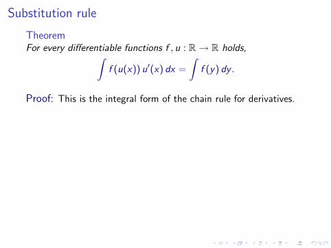
Substitution rule
TheoremFor every differentiable functions f , u : R → R holds,∫
f (u(x)) u′(x) dx =
∫f (y) dy .
Proof: This is the integral form of the chain rule for derivatives.
Let F be a primitive of f , that is, F ′ = f . Then(F (u)
)′= F ′(u) u′ = f (u) u′.
Integrate the equation above,∫f (u(x)) u′(x) dx =
∫d(F (u))
dx(x) dx = F (u(x)).
Denoting y = u(x), we get∫f (u(x)) u′(x) dx = F (y) =
∫F ′(y) dy =
∫f (y) dy .

Substitution rule
TheoremFor every differentiable functions f , u : R → R holds,∫
f (u(x)) u′(x) dx =
∫f (y) dy .
Proof: This is the integral form of the chain rule for derivatives.Let F be a primitive of f ,
that is, F ′ = f . Then(F (u)
)′= F ′(u) u′ = f (u) u′.
Integrate the equation above,∫f (u(x)) u′(x) dx =
∫d(F (u))
dx(x) dx = F (u(x)).
Denoting y = u(x), we get∫f (u(x)) u′(x) dx = F (y) =
∫F ′(y) dy =
∫f (y) dy .

Substitution rule
TheoremFor every differentiable functions f , u : R → R holds,∫
f (u(x)) u′(x) dx =
∫f (y) dy .
Proof: This is the integral form of the chain rule for derivatives.Let F be a primitive of f , that is, F ′ = f .
Then(F (u)
)′= F ′(u) u′ = f (u) u′.
Integrate the equation above,∫f (u(x)) u′(x) dx =
∫d(F (u))
dx(x) dx = F (u(x)).
Denoting y = u(x), we get∫f (u(x)) u′(x) dx = F (y) =
∫F ′(y) dy =
∫f (y) dy .
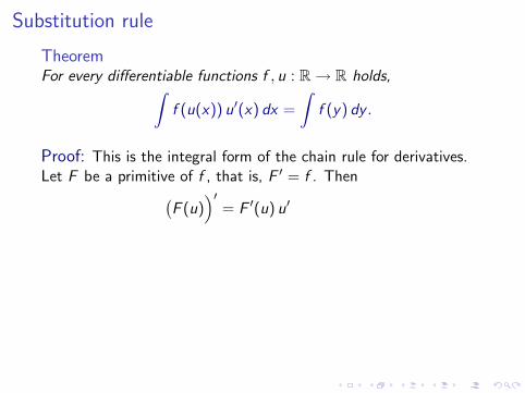
Substitution rule
TheoremFor every differentiable functions f , u : R → R holds,∫
f (u(x)) u′(x) dx =
∫f (y) dy .
Proof: This is the integral form of the chain rule for derivatives.Let F be a primitive of f , that is, F ′ = f . Then(
F (u))′
= F ′(u) u′
= f (u) u′.
Integrate the equation above,∫f (u(x)) u′(x) dx =
∫d(F (u))
dx(x) dx = F (u(x)).
Denoting y = u(x), we get∫f (u(x)) u′(x) dx = F (y) =
∫F ′(y) dy =
∫f (y) dy .

Substitution rule
TheoremFor every differentiable functions f , u : R → R holds,∫
f (u(x)) u′(x) dx =
∫f (y) dy .
Proof: This is the integral form of the chain rule for derivatives.Let F be a primitive of f , that is, F ′ = f . Then(
F (u))′
= F ′(u) u′ = f (u) u′.
Integrate the equation above,∫f (u(x)) u′(x) dx =
∫d(F (u))
dx(x) dx = F (u(x)).
Denoting y = u(x), we get∫f (u(x)) u′(x) dx = F (y) =
∫F ′(y) dy =
∫f (y) dy .
Substitution rule
TheoremFor every differentiable functions f , u : R → R holds,∫
f (u(x)) u′(x) dx =
∫f (y) dy .
Proof: This is the integral form of the chain rule for derivatives.Let F be a primitive of f , that is, F ′ = f . Then(
F (u))′
= F ′(u) u′ = f (u) u′.
Integrate the equation above,
∫f (u(x)) u′(x) dx =
∫d(F (u))
dx(x) dx = F (u(x)).
Denoting y = u(x), we get∫f (u(x)) u′(x) dx = F (y) =
∫F ′(y) dy =
∫f (y) dy .

Substitution rule
TheoremFor every differentiable functions f , u : R → R holds,∫
f (u(x)) u′(x) dx =
∫f (y) dy .
Proof: This is the integral form of the chain rule for derivatives.Let F be a primitive of f , that is, F ′ = f . Then(
F (u))′
= F ′(u) u′ = f (u) u′.
Integrate the equation above,∫f (u(x)) u′(x) dx =
∫d(F (u))
dx(x) dx
= F (u(x)).
Denoting y = u(x), we get∫f (u(x)) u′(x) dx = F (y) =
∫F ′(y) dy =
∫f (y) dy .

Substitution rule
TheoremFor every differentiable functions f , u : R → R holds,∫
f (u(x)) u′(x) dx =
∫f (y) dy .
Proof: This is the integral form of the chain rule for derivatives.Let F be a primitive of f , that is, F ′ = f . Then(
F (u))′
= F ′(u) u′ = f (u) u′.
Integrate the equation above,∫f (u(x)) u′(x) dx =
∫d(F (u))
dx(x) dx = F (u(x)).
Denoting y = u(x), we get∫f (u(x)) u′(x) dx = F (y) =
∫F ′(y) dy =
∫f (y) dy .

Substitution rule
TheoremFor every differentiable functions f , u : R → R holds,∫
f (u(x)) u′(x) dx =
∫f (y) dy .
Proof: This is the integral form of the chain rule for derivatives.Let F be a primitive of f , that is, F ′ = f . Then(
F (u))′
= F ′(u) u′ = f (u) u′.
Integrate the equation above,∫f (u(x)) u′(x) dx =
∫d(F (u))
dx(x) dx = F (u(x)).
Denoting y = u(x), we get
∫f (u(x)) u′(x) dx = F (y) =
∫F ′(y) dy =
∫f (y) dy .

Substitution rule
TheoremFor every differentiable functions f , u : R → R holds,∫
f (u(x)) u′(x) dx =
∫f (y) dy .
Proof: This is the integral form of the chain rule for derivatives.Let F be a primitive of f , that is, F ′ = f . Then(
F (u))′
= F ′(u) u′ = f (u) u′.
Integrate the equation above,∫f (u(x)) u′(x) dx =
∫d(F (u))
dx(x) dx = F (u(x)).
Denoting y = u(x), we get∫f (u(x)) u′(x) dx = F (y)
=
∫F ′(y) dy =
∫f (y) dy .

Substitution rule
TheoremFor every differentiable functions f , u : R → R holds,∫
f (u(x)) u′(x) dx =
∫f (y) dy .
Proof: This is the integral form of the chain rule for derivatives.Let F be a primitive of f , that is, F ′ = f . Then(
F (u))′
= F ′(u) u′ = f (u) u′.
Integrate the equation above,∫f (u(x)) u′(x) dx =
∫d(F (u))
dx(x) dx = F (u(x)).
Denoting y = u(x), we get∫f (u(x)) u′(x) dx = F (y) =
∫F ′(y) dy
=
∫f (y) dy .

Substitution rule
TheoremFor every differentiable functions f , u : R → R holds,∫
f (u(x)) u′(x) dx =
∫f (y) dy .
Proof: This is the integral form of the chain rule for derivatives.Let F be a primitive of f , that is, F ′ = f . Then(
F (u))′
= F ′(u) u′ = f (u) u′.
Integrate the equation above,∫f (u(x)) u′(x) dx =
∫d(F (u))
dx(x) dx = F (u(x)).
Denoting y = u(x), we get∫f (u(x)) u′(x) dx = F (y) =
∫F ′(y) dy =
∫f (y) dy .

Substitution rule
Example
Evaluate I =
∫3x etan(2x2)
[1 + cos(4x2)]dx .
Solution: The argument in the tangent function is has an x2,and in the integral appears the factor x dx . We try the substitution
u = tan(2x2), du =1
cos2(2x2)(4x) dx .
This substitution will simplify the integration if cos2(2x2) can berelated to [1 + cos(4x2)]. And this is the case, since
cos2(θ) =1
2
(1 + cos(2θ)
), θ = 2x2,
I =
∫3x etan(2x2)
[1 + cos(4x2)]dx =
∫3x etan(2x2)
2 cos2(2x2)dx =
3
2
∫eu du
4.

Substitution rule
Example
Evaluate I =
∫3x etan(2x2)
[1 + cos(4x2)]dx .
Solution: The argument in the tangent function is has an x2,
and in the integral appears the factor x dx . We try the substitution
u = tan(2x2), du =1
cos2(2x2)(4x) dx .
This substitution will simplify the integration if cos2(2x2) can berelated to [1 + cos(4x2)]. And this is the case, since
cos2(θ) =1
2
(1 + cos(2θ)
), θ = 2x2,
I =
∫3x etan(2x2)
[1 + cos(4x2)]dx =
∫3x etan(2x2)
2 cos2(2x2)dx =
3
2
∫eu du
4.

Substitution rule
Example
Evaluate I =
∫3x etan(2x2)
[1 + cos(4x2)]dx .
Solution: The argument in the tangent function is has an x2,and in the integral appears the factor x dx .
We try the substitution
u = tan(2x2), du =1
cos2(2x2)(4x) dx .
This substitution will simplify the integration if cos2(2x2) can berelated to [1 + cos(4x2)]. And this is the case, since
cos2(θ) =1
2
(1 + cos(2θ)
), θ = 2x2,
I =
∫3x etan(2x2)
[1 + cos(4x2)]dx =
∫3x etan(2x2)
2 cos2(2x2)dx =
3
2
∫eu du
4.

Substitution rule
Example
Evaluate I =
∫3x etan(2x2)
[1 + cos(4x2)]dx .
Solution: The argument in the tangent function is has an x2,and in the integral appears the factor x dx . We try the substitution
u = tan(2x2),
du =1
cos2(2x2)(4x) dx .
This substitution will simplify the integration if cos2(2x2) can berelated to [1 + cos(4x2)]. And this is the case, since
cos2(θ) =1
2
(1 + cos(2θ)
), θ = 2x2,
I =
∫3x etan(2x2)
[1 + cos(4x2)]dx =
∫3x etan(2x2)
2 cos2(2x2)dx =
3
2
∫eu du
4.

Substitution rule
Example
Evaluate I =
∫3x etan(2x2)
[1 + cos(4x2)]dx .
Solution: The argument in the tangent function is has an x2,and in the integral appears the factor x dx . We try the substitution
u = tan(2x2), du =1
cos2(2x2)(4x) dx .
This substitution will simplify the integration if cos2(2x2) can berelated to [1 + cos(4x2)]. And this is the case, since
cos2(θ) =1
2
(1 + cos(2θ)
), θ = 2x2,
I =
∫3x etan(2x2)
[1 + cos(4x2)]dx =
∫3x etan(2x2)
2 cos2(2x2)dx =
3
2
∫eu du
4.

Substitution rule
Example
Evaluate I =
∫3x etan(2x2)
[1 + cos(4x2)]dx .
Solution: The argument in the tangent function is has an x2,and in the integral appears the factor x dx . We try the substitution
u = tan(2x2), du =1
cos2(2x2)(4x) dx .
This substitution will simplify the integration if cos2(2x2) can berelated to [1 + cos(4x2)].
And this is the case, since
cos2(θ) =1
2
(1 + cos(2θ)
), θ = 2x2,
I =
∫3x etan(2x2)
[1 + cos(4x2)]dx =
∫3x etan(2x2)
2 cos2(2x2)dx =
3
2
∫eu du
4.

Substitution rule
Example
Evaluate I =
∫3x etan(2x2)
[1 + cos(4x2)]dx .
Solution: The argument in the tangent function is has an x2,and in the integral appears the factor x dx . We try the substitution
u = tan(2x2), du =1
cos2(2x2)(4x) dx .
This substitution will simplify the integration if cos2(2x2) can berelated to [1 + cos(4x2)]. And this is the case,
since
cos2(θ) =1
2
(1 + cos(2θ)
), θ = 2x2,
I =
∫3x etan(2x2)
[1 + cos(4x2)]dx =
∫3x etan(2x2)
2 cos2(2x2)dx =
3
2
∫eu du
4.

Substitution rule
Example
Evaluate I =
∫3x etan(2x2)
[1 + cos(4x2)]dx .
Solution: The argument in the tangent function is has an x2,and in the integral appears the factor x dx . We try the substitution
u = tan(2x2), du =1
cos2(2x2)(4x) dx .
This substitution will simplify the integration if cos2(2x2) can berelated to [1 + cos(4x2)]. And this is the case, since
cos2(θ) =1
2
(1 + cos(2θ)
),
θ = 2x2,
I =
∫3x etan(2x2)
[1 + cos(4x2)]dx =
∫3x etan(2x2)
2 cos2(2x2)dx =
3
2
∫eu du
4.

Substitution rule
Example
Evaluate I =
∫3x etan(2x2)
[1 + cos(4x2)]dx .
Solution: The argument in the tangent function is has an x2,and in the integral appears the factor x dx . We try the substitution
u = tan(2x2), du =1
cos2(2x2)(4x) dx .
This substitution will simplify the integration if cos2(2x2) can berelated to [1 + cos(4x2)]. And this is the case, since
cos2(θ) =1
2
(1 + cos(2θ)
), θ = 2x2,
I =
∫3x etan(2x2)
[1 + cos(4x2)]dx =
∫3x etan(2x2)
2 cos2(2x2)dx =
3
2
∫eu du
4.

Substitution rule
Example
Evaluate I =
∫3x etan(2x2)
[1 + cos(4x2)]dx .
Solution: The argument in the tangent function is has an x2,and in the integral appears the factor x dx . We try the substitution
u = tan(2x2), du =1
cos2(2x2)(4x) dx .
This substitution will simplify the integration if cos2(2x2) can berelated to [1 + cos(4x2)]. And this is the case, since
cos2(θ) =1
2
(1 + cos(2θ)
), θ = 2x2,
I =
∫3x etan(2x2)
[1 + cos(4x2)]dx
=
∫3x etan(2x2)
2 cos2(2x2)dx =
3
2
∫eu du
4.

Substitution rule
Example
Evaluate I =
∫3x etan(2x2)
[1 + cos(4x2)]dx .
Solution: The argument in the tangent function is has an x2,and in the integral appears the factor x dx . We try the substitution
u = tan(2x2), du =1
cos2(2x2)(4x) dx .
This substitution will simplify the integration if cos2(2x2) can berelated to [1 + cos(4x2)]. And this is the case, since
cos2(θ) =1
2
(1 + cos(2θ)
), θ = 2x2,
I =
∫3x etan(2x2)
[1 + cos(4x2)]dx =
∫3x etan(2x2)
2 cos2(2x2)dx
=3
2
∫eu du
4.

Substitution rule
Example
Evaluate I =
∫3x etan(2x2)
[1 + cos(4x2)]dx .
Solution: The argument in the tangent function is has an x2,and in the integral appears the factor x dx . We try the substitution
u = tan(2x2), du =1
cos2(2x2)(4x) dx .
This substitution will simplify the integration if cos2(2x2) can berelated to [1 + cos(4x2)]. And this is the case, since
cos2(θ) =1
2
(1 + cos(2θ)
), θ = 2x2,
I =
∫3x etan(2x2)
[1 + cos(4x2)]dx =
∫3x etan(2x2)
2 cos2(2x2)dx =
3
2
∫eu du
4.

Substitution rule
Example
Evaluate I =
∫3x etan(2x2)
[1 + cos(4x2)]dx .
Solution: Recall: I =3
2
∫eu du
4, with u = tan(2x2).
I =3
8
∫eu du =
3
8eu + c .
We now substitute back with u = tan(2x2),
I =3
8etan(2x2) + c .
C

Substitution rule
Example
Evaluate I =
∫3x etan(2x2)
[1 + cos(4x2)]dx .
Solution: Recall: I =3
2
∫eu du
4, with u = tan(2x2).
I =3
8
∫eu du
=3
8eu + c .
We now substitute back with u = tan(2x2),
I =3
8etan(2x2) + c .
C

Substitution rule
Example
Evaluate I =
∫3x etan(2x2)
[1 + cos(4x2)]dx .
Solution: Recall: I =3
2
∫eu du
4, with u = tan(2x2).
I =3
8
∫eu du =
3
8eu + c .
We now substitute back with u = tan(2x2),
I =3
8etan(2x2) + c .
C

Substitution rule
Example
Evaluate I =
∫3x etan(2x2)
[1 + cos(4x2)]dx .
Solution: Recall: I =3
2
∫eu du
4, with u = tan(2x2).
I =3
8
∫eu du =
3
8eu + c .
We now substitute back with u = tan(2x2),
I =3
8etan(2x2) + c .
C

Substitution rule
Example
Evaluate I =
∫3x etan(2x2)
[1 + cos(4x2)]dx .
Solution: Recall: I =3
2
∫eu du
4, with u = tan(2x2).
I =3
8
∫eu du =
3
8eu + c .
We now substitute back with u = tan(2x2),
I =3
8etan(2x2) + c .
C

Integration techniques (Supp. Material 8-IT)
I Substitution rule.
I Completing the square.
I Trigonometric identities.
I Polynomial division.
I Multiplying by 1.
Completing the square
Example
Evaluate I =
∫dx
(x + 3)√
x2 + 6x + 4.
Solution: The idea is to rewrite the function inside the square root:
x2 + 6x + 4 = x2 + 2(6
2
)x + 4 = x2 + 2(3x) + 4
x2 + 6x + 4 = [x2 + 2(3x) + 9]− 9 + 4 = (x + 3)2 − 5.
I =
∫dx
(x + 3)√
(x + 3)2 − 5u = x + 3, du = dx
I =
∫du
u√
u2 − 5=
1√5
arcsec( |u|√
5
)+ c .
We obtain I =1√5
arcsec( |x + 3|√
5
)+ c . C

Completing the square
Example
Evaluate I =
∫dx
(x + 3)√
x2 + 6x + 4.
Solution: The idea is to rewrite the function inside the square root:
x2 + 6x + 4
= x2 + 2(6
2
)x + 4 = x2 + 2(3x) + 4
x2 + 6x + 4 = [x2 + 2(3x) + 9]− 9 + 4 = (x + 3)2 − 5.
I =
∫dx
(x + 3)√
(x + 3)2 − 5u = x + 3, du = dx
I =
∫du
u√
u2 − 5=
1√5
arcsec( |u|√
5
)+ c .
We obtain I =1√5
arcsec( |x + 3|√
5
)+ c . C

Completing the square
Example
Evaluate I =
∫dx
(x + 3)√
x2 + 6x + 4.
Solution: The idea is to rewrite the function inside the square root:
x2 + 6x + 4 = x2 + 2(6
2
)x + 4
= x2 + 2(3x) + 4
x2 + 6x + 4 = [x2 + 2(3x) + 9]− 9 + 4 = (x + 3)2 − 5.
I =
∫dx
(x + 3)√
(x + 3)2 − 5u = x + 3, du = dx
I =
∫du
u√
u2 − 5=
1√5
arcsec( |u|√
5
)+ c .
We obtain I =1√5
arcsec( |x + 3|√
5
)+ c . C
Completing the square
Example
Evaluate I =
∫dx
(x + 3)√
x2 + 6x + 4.
Solution: The idea is to rewrite the function inside the square root:
x2 + 6x + 4 = x2 + 2(6
2
)x + 4 = x2 + 2(3x) + 4
x2 + 6x + 4 = [x2 + 2(3x) + 9]− 9 + 4 = (x + 3)2 − 5.
I =
∫dx
(x + 3)√
(x + 3)2 − 5u = x + 3, du = dx
I =
∫du
u√
u2 − 5=
1√5
arcsec( |u|√
5
)+ c .
We obtain I =1√5
arcsec( |x + 3|√
5
)+ c . C
Completing the square
Example
Evaluate I =
∫dx
(x + 3)√
x2 + 6x + 4.
Solution: The idea is to rewrite the function inside the square root:
x2 + 6x + 4 = x2 + 2(6
2
)x + 4 = x2 + 2(3x) + 4
x2 + 6x + 4 = [x2 + 2(3x) + 9]− 9 + 4
= (x + 3)2 − 5.
I =
∫dx
(x + 3)√
(x + 3)2 − 5u = x + 3, du = dx
I =
∫du
u√
u2 − 5=
1√5
arcsec( |u|√
5
)+ c .
We obtain I =1√5
arcsec( |x + 3|√
5
)+ c . C

Completing the square
Example
Evaluate I =
∫dx
(x + 3)√
x2 + 6x + 4.
Solution: The idea is to rewrite the function inside the square root:
x2 + 6x + 4 = x2 + 2(6
2
)x + 4 = x2 + 2(3x) + 4
x2 + 6x + 4 = [x2 + 2(3x) + 9]− 9 + 4 = (x + 3)2 − 5.
I =
∫dx
(x + 3)√
(x + 3)2 − 5u = x + 3, du = dx
I =
∫du
u√
u2 − 5=
1√5
arcsec( |u|√
5
)+ c .
We obtain I =1√5
arcsec( |x + 3|√
5
)+ c . C

Completing the square
Example
Evaluate I =
∫dx
(x + 3)√
x2 + 6x + 4.
Solution: The idea is to rewrite the function inside the square root:
x2 + 6x + 4 = x2 + 2(6
2
)x + 4 = x2 + 2(3x) + 4
x2 + 6x + 4 = [x2 + 2(3x) + 9]− 9 + 4 = (x + 3)2 − 5.
I =
∫dx
(x + 3)√
(x + 3)2 − 5
u = x + 3, du = dx
I =
∫du
u√
u2 − 5=
1√5
arcsec( |u|√
5
)+ c .
We obtain I =1√5
arcsec( |x + 3|√
5
)+ c . C

Completing the square
Example
Evaluate I =
∫dx
(x + 3)√
x2 + 6x + 4.
Solution: The idea is to rewrite the function inside the square root:
x2 + 6x + 4 = x2 + 2(6
2
)x + 4 = x2 + 2(3x) + 4
x2 + 6x + 4 = [x2 + 2(3x) + 9]− 9 + 4 = (x + 3)2 − 5.
I =
∫dx
(x + 3)√
(x + 3)2 − 5u = x + 3,
du = dx
I =
∫du
u√
u2 − 5=
1√5
arcsec( |u|√
5
)+ c .
We obtain I =1√5
arcsec( |x + 3|√
5
)+ c . C

Completing the square
Example
Evaluate I =
∫dx
(x + 3)√
x2 + 6x + 4.
Solution: The idea is to rewrite the function inside the square root:
x2 + 6x + 4 = x2 + 2(6
2
)x + 4 = x2 + 2(3x) + 4
x2 + 6x + 4 = [x2 + 2(3x) + 9]− 9 + 4 = (x + 3)2 − 5.
I =
∫dx
(x + 3)√
(x + 3)2 − 5u = x + 3, du = dx
I =
∫du
u√
u2 − 5=
1√5
arcsec( |u|√
5
)+ c .
We obtain I =1√5
arcsec( |x + 3|√
5
)+ c . C
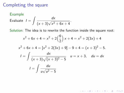
Completing the square
Example
Evaluate I =
∫dx
(x + 3)√
x2 + 6x + 4.
Solution: The idea is to rewrite the function inside the square root:
x2 + 6x + 4 = x2 + 2(6
2
)x + 4 = x2 + 2(3x) + 4
x2 + 6x + 4 = [x2 + 2(3x) + 9]− 9 + 4 = (x + 3)2 − 5.
I =
∫dx
(x + 3)√
(x + 3)2 − 5u = x + 3, du = dx
I =
∫du
u√
u2 − 5
=1√5
arcsec( |u|√
5
)+ c .
We obtain I =1√5
arcsec( |x + 3|√
5
)+ c . C
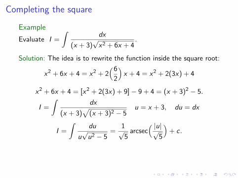
Completing the square
Example
Evaluate I =
∫dx
(x + 3)√
x2 + 6x + 4.
Solution: The idea is to rewrite the function inside the square root:
x2 + 6x + 4 = x2 + 2(6
2
)x + 4 = x2 + 2(3x) + 4
x2 + 6x + 4 = [x2 + 2(3x) + 9]− 9 + 4 = (x + 3)2 − 5.
I =
∫dx
(x + 3)√
(x + 3)2 − 5u = x + 3, du = dx
I =
∫du
u√
u2 − 5=
1√5
arcsec( |u|√
5
)+ c .
We obtain I =1√5
arcsec( |x + 3|√
5
)+ c . C

Completing the square
Example
Evaluate I =
∫dx
(x + 3)√
x2 + 6x + 4.
Solution: The idea is to rewrite the function inside the square root:
x2 + 6x + 4 = x2 + 2(6
2
)x + 4 = x2 + 2(3x) + 4
x2 + 6x + 4 = [x2 + 2(3x) + 9]− 9 + 4 = (x + 3)2 − 5.
I =
∫dx
(x + 3)√
(x + 3)2 − 5u = x + 3, du = dx
I =
∫du
u√
u2 − 5=
1√5
arcsec( |u|√
5
)+ c .
We obtain I =1√5
arcsec( |x + 3|√
5
)+ c . C

Completing the square
Remark: Sometimes completing the square is not needed.
Example
Evaluate I =
∫(x + 3) dx√x2 + 6x + 4
.
Solution: Since the factor (x + 3) is in the numerator, instead ofthe denominator, substitution will work:
u = x2 + 6x + 4, du = (2x + 6) dx = 2(x + 3) dx .
I =
∫1√u
du
2=
1
2
∫u−1/2 du =
1
2
(2u1/2
)+ c .
We conclude that I =√
x2 + 6x + 4 + c . C

Completing the square
Remark: Sometimes completing the square is not needed.
Example
Evaluate I =
∫(x + 3) dx√x2 + 6x + 4
.
Solution: Since the factor (x + 3) is in the numerator, instead ofthe denominator,
substitution will work:
u = x2 + 6x + 4, du = (2x + 6) dx = 2(x + 3) dx .
I =
∫1√u
du
2=
1
2
∫u−1/2 du =
1
2
(2u1/2
)+ c .
We conclude that I =√
x2 + 6x + 4 + c . C

Completing the square
Remark: Sometimes completing the square is not needed.
Example
Evaluate I =
∫(x + 3) dx√x2 + 6x + 4
.
Solution: Since the factor (x + 3) is in the numerator, instead ofthe denominator, substitution will work:
u = x2 + 6x + 4, du = (2x + 6) dx = 2(x + 3) dx .
I =
∫1√u
du
2=
1
2
∫u−1/2 du =
1
2
(2u1/2
)+ c .
We conclude that I =√
x2 + 6x + 4 + c . C

Completing the square
Remark: Sometimes completing the square is not needed.
Example
Evaluate I =
∫(x + 3) dx√x2 + 6x + 4
.
Solution: Since the factor (x + 3) is in the numerator, instead ofthe denominator, substitution will work:
u = x2 + 6x + 4,
du = (2x + 6) dx = 2(x + 3) dx .
I =
∫1√u
du
2=
1
2
∫u−1/2 du =
1
2
(2u1/2
)+ c .
We conclude that I =√
x2 + 6x + 4 + c . C

Completing the square
Remark: Sometimes completing the square is not needed.
Example
Evaluate I =
∫(x + 3) dx√x2 + 6x + 4
.
Solution: Since the factor (x + 3) is in the numerator, instead ofthe denominator, substitution will work:
u = x2 + 6x + 4, du = (2x + 6) dx
= 2(x + 3) dx .
I =
∫1√u
du
2=
1
2
∫u−1/2 du =
1
2
(2u1/2
)+ c .
We conclude that I =√
x2 + 6x + 4 + c . C

Completing the square
Remark: Sometimes completing the square is not needed.
Example
Evaluate I =
∫(x + 3) dx√x2 + 6x + 4
.
Solution: Since the factor (x + 3) is in the numerator, instead ofthe denominator, substitution will work:
u = x2 + 6x + 4, du = (2x + 6) dx = 2(x + 3) dx .
I =
∫1√u
du
2=
1
2
∫u−1/2 du =
1
2
(2u1/2
)+ c .
We conclude that I =√
x2 + 6x + 4 + c . C

Completing the square
Remark: Sometimes completing the square is not needed.
Example
Evaluate I =
∫(x + 3) dx√x2 + 6x + 4
.
Solution: Since the factor (x + 3) is in the numerator, instead ofthe denominator, substitution will work:
u = x2 + 6x + 4, du = (2x + 6) dx = 2(x + 3) dx .
I =
∫1√u
du
2
=1
2
∫u−1/2 du =
1
2
(2u1/2
)+ c .
We conclude that I =√
x2 + 6x + 4 + c . C

Completing the square
Remark: Sometimes completing the square is not needed.
Example
Evaluate I =
∫(x + 3) dx√x2 + 6x + 4
.
Solution: Since the factor (x + 3) is in the numerator, instead ofthe denominator, substitution will work:
u = x2 + 6x + 4, du = (2x + 6) dx = 2(x + 3) dx .
I =
∫1√u
du
2=
1
2
∫u−1/2 du
=1
2
(2u1/2
)+ c .
We conclude that I =√
x2 + 6x + 4 + c . C

Completing the square
Remark: Sometimes completing the square is not needed.
Example
Evaluate I =
∫(x + 3) dx√x2 + 6x + 4
.
Solution: Since the factor (x + 3) is in the numerator, instead ofthe denominator, substitution will work:
u = x2 + 6x + 4, du = (2x + 6) dx = 2(x + 3) dx .
I =
∫1√u
du
2=
1
2
∫u−1/2 du =
1
2
(2u1/2
)+ c .
We conclude that I =√
x2 + 6x + 4 + c . C

Completing the square
Remark: Sometimes completing the square is not needed.
Example
Evaluate I =
∫(x + 3) dx√x2 + 6x + 4
.
Solution: Since the factor (x + 3) is in the numerator, instead ofthe denominator, substitution will work:
u = x2 + 6x + 4, du = (2x + 6) dx = 2(x + 3) dx .
I =
∫1√u
du
2=
1
2
∫u−1/2 du =
1
2
(2u1/2
)+ c .
We conclude that I =√
x2 + 6x + 4 + c . C

Integration techniques (Supp. Material 8-IT)
I Substitution rule.
I Completing the square.
I Trigonometric identities.
I Polynomial division.
I Multiplying by 1.

Trigonometric identities
Example
Evaluate I =
∫ [sec(x) + tan(x)
]2dx .
Solution: This problem can be solved using trigonometric identitiesfor sine and cosine functions only.
f (x) =[sec(x) + tan(x)
]2=
[ 1
cos(x)+
sin(x)
cos(x)
]2=
(1 + sin(x))2
cos2(x).
f (x) =1 + 2 sin(x) + sin2(x)
cos2(x)=
1
cos2(x)+
2 sin(x)
cos2(x)+
sin2(x)
cos2(x).
sin2(x)
cos2(x)=
1− cos2(x)
cos2(x)=
1
cos2(x)− 1.

Trigonometric identities
Example
Evaluate I =
∫ [sec(x) + tan(x)
]2dx .
Solution: This problem can be solved using trigonometric identitiesfor sine and cosine functions only.
f (x) =[sec(x) + tan(x)
]2
=[ 1
cos(x)+
sin(x)
cos(x)
]2=
(1 + sin(x))2
cos2(x).
f (x) =1 + 2 sin(x) + sin2(x)
cos2(x)=
1
cos2(x)+
2 sin(x)
cos2(x)+
sin2(x)
cos2(x).
sin2(x)
cos2(x)=
1− cos2(x)
cos2(x)=
1
cos2(x)− 1.

Trigonometric identities
Example
Evaluate I =
∫ [sec(x) + tan(x)
]2dx .
Solution: This problem can be solved using trigonometric identitiesfor sine and cosine functions only.
f (x) =[sec(x) + tan(x)
]2=
[ 1
cos(x)+
sin(x)
cos(x)
]2
=(1 + sin(x))2
cos2(x).
f (x) =1 + 2 sin(x) + sin2(x)
cos2(x)=
1
cos2(x)+
2 sin(x)
cos2(x)+
sin2(x)
cos2(x).
sin2(x)
cos2(x)=
1− cos2(x)
cos2(x)=
1
cos2(x)− 1.

Trigonometric identities
Example
Evaluate I =
∫ [sec(x) + tan(x)
]2dx .
Solution: This problem can be solved using trigonometric identitiesfor sine and cosine functions only.
f (x) =[sec(x) + tan(x)
]2=
[ 1
cos(x)+
sin(x)
cos(x)
]2=
(1 + sin(x))2
cos2(x).
f (x) =1 + 2 sin(x) + sin2(x)
cos2(x)=
1
cos2(x)+
2 sin(x)
cos2(x)+
sin2(x)
cos2(x).
sin2(x)
cos2(x)=
1− cos2(x)
cos2(x)=
1
cos2(x)− 1.

Trigonometric identities
Example
Evaluate I =
∫ [sec(x) + tan(x)
]2dx .
Solution: This problem can be solved using trigonometric identitiesfor sine and cosine functions only.
f (x) =[sec(x) + tan(x)
]2=
[ 1
cos(x)+
sin(x)
cos(x)
]2=
(1 + sin(x))2
cos2(x).
f (x) =1 + 2 sin(x) + sin2(x)
cos2(x)
=1
cos2(x)+
2 sin(x)
cos2(x)+
sin2(x)
cos2(x).
sin2(x)
cos2(x)=
1− cos2(x)
cos2(x)=
1
cos2(x)− 1.

Trigonometric identities
Example
Evaluate I =
∫ [sec(x) + tan(x)
]2dx .
Solution: This problem can be solved using trigonometric identitiesfor sine and cosine functions only.
f (x) =[sec(x) + tan(x)
]2=
[ 1
cos(x)+
sin(x)
cos(x)
]2=
(1 + sin(x))2
cos2(x).
f (x) =1 + 2 sin(x) + sin2(x)
cos2(x)=
1
cos2(x)+
2 sin(x)
cos2(x)+
sin2(x)
cos2(x).
sin2(x)
cos2(x)=
1− cos2(x)
cos2(x)=
1
cos2(x)− 1.
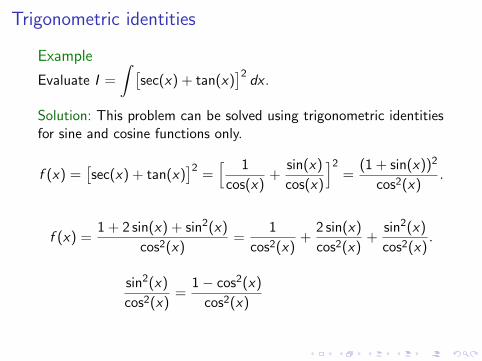
Trigonometric identities
Example
Evaluate I =
∫ [sec(x) + tan(x)
]2dx .
Solution: This problem can be solved using trigonometric identitiesfor sine and cosine functions only.
f (x) =[sec(x) + tan(x)
]2=
[ 1
cos(x)+
sin(x)
cos(x)
]2=
(1 + sin(x))2
cos2(x).
f (x) =1 + 2 sin(x) + sin2(x)
cos2(x)=
1
cos2(x)+
2 sin(x)
cos2(x)+
sin2(x)
cos2(x).
sin2(x)
cos2(x)=
1− cos2(x)
cos2(x)
=1
cos2(x)− 1.

Trigonometric identities
Example
Evaluate I =
∫ [sec(x) + tan(x)
]2dx .
Solution: This problem can be solved using trigonometric identitiesfor sine and cosine functions only.
f (x) =[sec(x) + tan(x)
]2=
[ 1
cos(x)+
sin(x)
cos(x)
]2=
(1 + sin(x))2
cos2(x).
f (x) =1 + 2 sin(x) + sin2(x)
cos2(x)=
1
cos2(x)+
2 sin(x)
cos2(x)+
sin2(x)
cos2(x).
sin2(x)
cos2(x)=
1− cos2(x)
cos2(x)=
1
cos2(x)− 1.

Trigonometric identities
Example
Evaluate I =
∫ [sec(x) + tan(x)
]2dx .
Solution: Recall: f (x) =[sec(x) + tan(x)
]2,
f (x) =1
cos2(x)+
2 sin(x)
cos2(x)+
sin2(x)
cos2(x)and
sin2(x)
cos2(x)=
1
cos2(x)− 1.
f (x) =2
cos2(x)+
2 sin(x)
cos2(x)− 1.
I =
∫2 dx
cos2(x)+
∫2 sin(x) dx
cos2(x)−
∫dx .
u = cos(x),
du = − sin(x) dx .
I = 2 tan(x)− 2
∫du
u2− x + c ⇒ I = 2 tan(x) +
2
cos(x)− x + c .
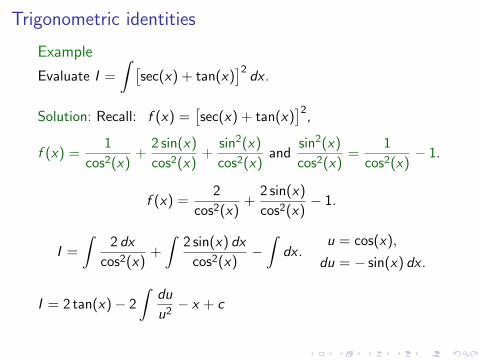
Trigonometric identities
Example
Evaluate I =
∫ [sec(x) + tan(x)
]2dx .
Solution: Recall: f (x) =[sec(x) + tan(x)
]2,
f (x) =1
cos2(x)+
2 sin(x)
cos2(x)+
sin2(x)
cos2(x)and
sin2(x)
cos2(x)=
1
cos2(x)− 1.
f (x) =2
cos2(x)+
2 sin(x)
cos2(x)− 1.
I =
∫2 dx
cos2(x)+
∫2 sin(x) dx
cos2(x)−
∫dx .
u = cos(x),
du = − sin(x) dx .
I = 2 tan(x)− 2
∫du
u2− x + c
⇒ I = 2 tan(x) +2
cos(x)− x + c .

Trigonometric identities
Example
Evaluate I =
∫ [sec(x) + tan(x)
]2dx .
Solution: Recall: f (x) =[sec(x) + tan(x)
]2,
f (x) =1
cos2(x)+
2 sin(x)
cos2(x)+
sin2(x)
cos2(x)and
sin2(x)
cos2(x)=
1
cos2(x)− 1.
f (x) =2
cos2(x)+
2 sin(x)
cos2(x)− 1.
I =
∫2 dx
cos2(x)+
∫2 sin(x) dx
cos2(x)−
∫dx .
u = cos(x),
du = − sin(x) dx .
I = 2 tan(x)− 2
∫du
u2− x + c ⇒ I = 2 tan(x) +
2
cos(x)− x + c .
Integration techniques (Supp. Material 8-IT)
I Substitution rule.
I Completing the square.
I Trigonometric identities.
I Polynomial division.
I Multiplying by 1.

Polynomial division
Example
Evaluate I =
∫4x2 − 7
2x + 3dx .
Solution: The degree of the polynomial in the numerator is greateror equal the degree of the polynomial in the denominator.In this case it is convenient to do the division:
2x − 3
2x + 3)
4x2 − 7− 4x2 − 6x
− 6x − 76x + 9
2
⇒ 4x2 − 7
2x + 3= 2x − 3 +
2
2x + 3.
I =
∫(2x−3) dx +
∫2 dx
2x + 3⇒ I = x2−3x +ln(2x +3)+ c .

Polynomial division
Example
Evaluate I =
∫4x2 − 7
2x + 3dx .
Solution: The degree of the polynomial in the numerator is greateror equal the degree of the polynomial in the denominator.
In this case it is convenient to do the division:
2x − 3
2x + 3)
4x2 − 7− 4x2 − 6x
− 6x − 76x + 9
2
⇒ 4x2 − 7
2x + 3= 2x − 3 +
2
2x + 3.
I =
∫(2x−3) dx +
∫2 dx
2x + 3⇒ I = x2−3x +ln(2x +3)+ c .

Polynomial division
Example
Evaluate I =
∫4x2 − 7
2x + 3dx .
Solution: The degree of the polynomial in the numerator is greateror equal the degree of the polynomial in the denominator.In this case it is convenient to do the division:
2x − 3
2x + 3)
4x2 − 7− 4x2 − 6x
− 6x − 76x + 9
2
⇒ 4x2 − 7
2x + 3= 2x − 3 +
2
2x + 3.
I =
∫(2x−3) dx +
∫2 dx
2x + 3⇒ I = x2−3x +ln(2x +3)+ c .

Polynomial division
Example
Evaluate I =
∫4x2 − 7
2x + 3dx .
Solution: The degree of the polynomial in the numerator is greateror equal the degree of the polynomial in the denominator.In this case it is convenient to do the division:
2x − 3
2x + 3)
4x2 − 7− 4x2 − 6x
− 6x − 76x + 9
2
⇒ 4x2 − 7
2x + 3= 2x − 3 +
2
2x + 3.
I =
∫(2x−3) dx +
∫2 dx
2x + 3
⇒ I = x2−3x +ln(2x +3)+ c .

Polynomial division
Example
Evaluate I =
∫4x2 − 7
2x + 3dx .
Solution: The degree of the polynomial in the numerator is greateror equal the degree of the polynomial in the denominator.In this case it is convenient to do the division:
2x − 3
2x + 3)
4x2 − 7− 4x2 − 6x
− 6x − 76x + 9
2
⇒ 4x2 − 7
2x + 3= 2x − 3 +
2
2x + 3.
I =
∫(2x−3) dx +
∫2 dx
2x + 3⇒ I = x2−3x +ln(2x +3)+ c .

Integration techniques (Supp. Material 8-IT)
I Substitution rule.
I Completing the square.
I Trigonometric identities.
I Polynomial division.
I Multiplying by 1.

Multiplying by 1
Example
Evaluate I =
∫dx
1 + sin(x).
Solution:
I =
∫1(
1 + sin(x)) (
1− sin(x))(
1− sin(x)) dx =
∫ (1− sin(x)
)(1− sin2(x)
) dx .
I =
∫ (1− sin(x)
)cos2(x)
dx =
∫dx
cos2(x)−
∫sin(x)
cos2(x)dx .
Since tan′(x) =1
cos2(x)and u = cos(x) implies du = − sin(x) dx ,
I = tan(x) +
∫du
u2= tan(x)− 1
u+ c = tan(x)− 1
cos(x)+ c .
We conclude that I = tan(x)− sec(x) + c . C

Multiplying by 1
Example
Evaluate I =
∫dx
1 + sin(x).
Solution:
I =
∫1(
1 + sin(x)) (
1− sin(x))(
1− sin(x)) dx
=
∫ (1− sin(x)
)(1− sin2(x)
) dx .
I =
∫ (1− sin(x)
)cos2(x)
dx =
∫dx
cos2(x)−
∫sin(x)
cos2(x)dx .
Since tan′(x) =1
cos2(x)and u = cos(x) implies du = − sin(x) dx ,
I = tan(x) +
∫du
u2= tan(x)− 1
u+ c = tan(x)− 1
cos(x)+ c .
We conclude that I = tan(x)− sec(x) + c . C

Multiplying by 1
Example
Evaluate I =
∫dx
1 + sin(x).
Solution:
I =
∫1(
1 + sin(x)) (
1− sin(x))(
1− sin(x)) dx =
∫ (1− sin(x)
)(1− sin2(x)
) dx .
I =
∫ (1− sin(x)
)cos2(x)
dx =
∫dx
cos2(x)−
∫sin(x)
cos2(x)dx .
Since tan′(x) =1
cos2(x)and u = cos(x) implies du = − sin(x) dx ,
I = tan(x) +
∫du
u2= tan(x)− 1
u+ c = tan(x)− 1
cos(x)+ c .
We conclude that I = tan(x)− sec(x) + c . C

Multiplying by 1
Example
Evaluate I =
∫dx
1 + sin(x).
Solution:
I =
∫1(
1 + sin(x)) (
1− sin(x))(
1− sin(x)) dx =
∫ (1− sin(x)
)(1− sin2(x)
) dx .
I =
∫ (1− sin(x)
)cos2(x)
dx
=
∫dx
cos2(x)−
∫sin(x)
cos2(x)dx .
Since tan′(x) =1
cos2(x)and u = cos(x) implies du = − sin(x) dx ,
I = tan(x) +
∫du
u2= tan(x)− 1
u+ c = tan(x)− 1
cos(x)+ c .
We conclude that I = tan(x)− sec(x) + c . C

Multiplying by 1
Example
Evaluate I =
∫dx
1 + sin(x).
Solution:
I =
∫1(
1 + sin(x)) (
1− sin(x))(
1− sin(x)) dx =
∫ (1− sin(x)
)(1− sin2(x)
) dx .
I =
∫ (1− sin(x)
)cos2(x)
dx =
∫dx
cos2(x)−
∫sin(x)
cos2(x)dx .
Since tan′(x) =1
cos2(x)and u = cos(x) implies du = − sin(x) dx ,
I = tan(x) +
∫du
u2= tan(x)− 1
u+ c = tan(x)− 1
cos(x)+ c .
We conclude that I = tan(x)− sec(x) + c . C

Multiplying by 1
Example
Evaluate I =
∫dx
1 + sin(x).
Solution:
I =
∫1(
1 + sin(x)) (
1− sin(x))(
1− sin(x)) dx =
∫ (1− sin(x)
)(1− sin2(x)
) dx .
I =
∫ (1− sin(x)
)cos2(x)
dx =
∫dx
cos2(x)−
∫sin(x)
cos2(x)dx .
Since tan′(x) =1
cos2(x)
and u = cos(x) implies du = − sin(x) dx ,
I = tan(x) +
∫du
u2= tan(x)− 1
u+ c = tan(x)− 1
cos(x)+ c .
We conclude that I = tan(x)− sec(x) + c . C

Multiplying by 1
Example
Evaluate I =
∫dx
1 + sin(x).
Solution:
I =
∫1(
1 + sin(x)) (
1− sin(x))(
1− sin(x)) dx =
∫ (1− sin(x)
)(1− sin2(x)
) dx .
I =
∫ (1− sin(x)
)cos2(x)
dx =
∫dx
cos2(x)−
∫sin(x)
cos2(x)dx .
Since tan′(x) =1
cos2(x)and u = cos(x)
implies du = − sin(x) dx ,
I = tan(x) +
∫du
u2= tan(x)− 1
u+ c = tan(x)− 1
cos(x)+ c .
We conclude that I = tan(x)− sec(x) + c . C

Multiplying by 1
Example
Evaluate I =
∫dx
1 + sin(x).
Solution:
I =
∫1(
1 + sin(x)) (
1− sin(x))(
1− sin(x)) dx =
∫ (1− sin(x)
)(1− sin2(x)
) dx .
I =
∫ (1− sin(x)
)cos2(x)
dx =
∫dx
cos2(x)−
∫sin(x)
cos2(x)dx .
Since tan′(x) =1
cos2(x)and u = cos(x) implies du = − sin(x) dx ,
I = tan(x) +
∫du
u2= tan(x)− 1
u+ c = tan(x)− 1
cos(x)+ c .
We conclude that I = tan(x)− sec(x) + c . C

Multiplying by 1
Example
Evaluate I =
∫dx
1 + sin(x).
Solution:
I =
∫1(
1 + sin(x)) (
1− sin(x))(
1− sin(x)) dx =
∫ (1− sin(x)
)(1− sin2(x)
) dx .
I =
∫ (1− sin(x)
)cos2(x)
dx =
∫dx
cos2(x)−
∫sin(x)
cos2(x)dx .
Since tan′(x) =1
cos2(x)and u = cos(x) implies du = − sin(x) dx ,
I = tan(x) +
∫du
u2
= tan(x)− 1
u+ c = tan(x)− 1
cos(x)+ c .
We conclude that I = tan(x)− sec(x) + c . C

Multiplying by 1
Example
Evaluate I =
∫dx
1 + sin(x).
Solution:
I =
∫1(
1 + sin(x)) (
1− sin(x))(
1− sin(x)) dx =
∫ (1− sin(x)
)(1− sin2(x)
) dx .
I =
∫ (1− sin(x)
)cos2(x)
dx =
∫dx
cos2(x)−
∫sin(x)
cos2(x)dx .
Since tan′(x) =1
cos2(x)and u = cos(x) implies du = − sin(x) dx ,
I = tan(x) +
∫du
u2= tan(x)− 1
u+ c
= tan(x)− 1
cos(x)+ c .
We conclude that I = tan(x)− sec(x) + c . C

Multiplying by 1
Example
Evaluate I =
∫dx
1 + sin(x).
Solution:
I =
∫1(
1 + sin(x)) (
1− sin(x))(
1− sin(x)) dx =
∫ (1− sin(x)
)(1− sin2(x)
) dx .
I =
∫ (1− sin(x)
)cos2(x)
dx =
∫dx
cos2(x)−
∫sin(x)
cos2(x)dx .
Since tan′(x) =1
cos2(x)and u = cos(x) implies du = − sin(x) dx ,
I = tan(x) +
∫du
u2= tan(x)− 1
u+ c = tan(x)− 1
cos(x)+ c .
We conclude that I = tan(x)− sec(x) + c . C

Multiplying by 1
Example
Evaluate I =
∫dx
1 + sin(x).
Solution:
I =
∫1(
1 + sin(x)) (
1− sin(x))(
1− sin(x)) dx =
∫ (1− sin(x)
)(1− sin2(x)
) dx .
I =
∫ (1− sin(x)
)cos2(x)
dx =
∫dx
cos2(x)−
∫sin(x)
cos2(x)dx .
Since tan′(x) =1
cos2(x)and u = cos(x) implies du = − sin(x) dx ,
I = tan(x) +
∫du
u2= tan(x)− 1
u+ c = tan(x)− 1
cos(x)+ c .
We conclude that I = tan(x)− sec(x) + c . C

Multiplying by 1
Example
Evaluate I =
∫sec(x) dx .
Solution: This problem can be solved using trigonometric identitiesfor sine and cosine functions only.
I =
∫dx
cos(x)=
∫1
cos(x)
(1
cos2(x)+ sin(x)
cos2(x)
)(
1cos2(x)
+ sin(x)cos2(x)
) dx
I =
∫ (1
cos2(x)+ sin(x)
cos2(x)
)(
1cos(x) + sin(x)
cos(x)
) dx and
( 1
cos(x)
)′=
sin(x)
cos2(x),( sin(x)
cos(x)
)′=
1
cos2(x).
I =
∫ (1
cos(x) + sin(x)cos(x)
)′(1
cos(x) + sin(x)cos(x)
) dx ⇒ I = ln( 1
cos(x)+
sin(x)
cos(x)
)+ c .

Multiplying by 1
Example
Evaluate I =
∫sec(x) dx .
Solution: This problem can be solved using trigonometric identitiesfor sine and cosine functions only.
I =
∫dx
cos(x)
=
∫1
cos(x)
(1
cos2(x)+ sin(x)
cos2(x)
)(
1cos2(x)
+ sin(x)cos2(x)
) dx
I =
∫ (1
cos2(x)+ sin(x)
cos2(x)
)(
1cos(x) + sin(x)
cos(x)
) dx and
( 1
cos(x)
)′=
sin(x)
cos2(x),( sin(x)
cos(x)
)′=
1
cos2(x).
I =
∫ (1
cos(x) + sin(x)cos(x)
)′(1
cos(x) + sin(x)cos(x)
) dx ⇒ I = ln( 1
cos(x)+
sin(x)
cos(x)
)+ c .

Multiplying by 1
Example
Evaluate I =
∫sec(x) dx .
Solution: This problem can be solved using trigonometric identitiesfor sine and cosine functions only.
I =
∫dx
cos(x)=
∫1
cos(x)
(1
cos2(x)+ sin(x)
cos2(x)
)(
1cos2(x)
+ sin(x)cos2(x)
) dx
I =
∫ (1
cos2(x)+ sin(x)
cos2(x)
)(
1cos(x) + sin(x)
cos(x)
) dx and
( 1
cos(x)
)′=
sin(x)
cos2(x),( sin(x)
cos(x)
)′=
1
cos2(x).
I =
∫ (1
cos(x) + sin(x)cos(x)
)′(1
cos(x) + sin(x)cos(x)
) dx ⇒ I = ln( 1
cos(x)+
sin(x)
cos(x)
)+ c .

Multiplying by 1
Example
Evaluate I =
∫sec(x) dx .
Solution: This problem can be solved using trigonometric identitiesfor sine and cosine functions only.
I =
∫dx
cos(x)=
∫1
cos(x)
(1
cos2(x)+ sin(x)
cos2(x)
)(
1cos2(x)
+ sin(x)cos2(x)
) dx
I =
∫ (1
cos2(x)+ sin(x)
cos2(x)
)(
1cos(x) + sin(x)
cos(x)
) dx
and
( 1
cos(x)
)′=
sin(x)
cos2(x),( sin(x)
cos(x)
)′=
1
cos2(x).
I =
∫ (1
cos(x) + sin(x)cos(x)
)′(1
cos(x) + sin(x)cos(x)
) dx ⇒ I = ln( 1
cos(x)+
sin(x)
cos(x)
)+ c .

Multiplying by 1
Example
Evaluate I =
∫sec(x) dx .
Solution: This problem can be solved using trigonometric identitiesfor sine and cosine functions only.
I =
∫dx
cos(x)=
∫1
cos(x)
(1
cos2(x)+ sin(x)
cos2(x)
)(
1cos2(x)
+ sin(x)cos2(x)
) dx
I =
∫ (1
cos2(x)+ sin(x)
cos2(x)
)(
1cos(x) + sin(x)
cos(x)
) dx and
( 1
cos(x)
)′=
sin(x)
cos2(x),( sin(x)
cos(x)
)′=
1
cos2(x).
I =
∫ (1
cos(x) + sin(x)cos(x)
)′(1
cos(x) + sin(x)cos(x)
) dx ⇒ I = ln( 1
cos(x)+
sin(x)
cos(x)
)+ c .

Multiplying by 1
Example
Evaluate I =
∫sec(x) dx .
Solution: This problem can be solved using trigonometric identitiesfor sine and cosine functions only.
I =
∫dx
cos(x)=
∫1
cos(x)
(1
cos2(x)+ sin(x)
cos2(x)
)(
1cos2(x)
+ sin(x)cos2(x)
) dx
I =
∫ (1
cos2(x)+ sin(x)
cos2(x)
)(
1cos(x) + sin(x)
cos(x)
) dx and
( 1
cos(x)
)′=
sin(x)
cos2(x),( sin(x)
cos(x)
)′=
1
cos2(x).
I =
∫ (1
cos(x) + sin(x)cos(x)
)′(1
cos(x) + sin(x)cos(x)
) dx
⇒ I = ln( 1
cos(x)+
sin(x)
cos(x)
)+ c .

Multiplying by 1
Example
Evaluate I =
∫sec(x) dx .
Solution: This problem can be solved using trigonometric identitiesfor sine and cosine functions only.
I =
∫dx
cos(x)=
∫1
cos(x)
(1
cos2(x)+ sin(x)
cos2(x)
)(
1cos2(x)
+ sin(x)cos2(x)
) dx
I =
∫ (1
cos2(x)+ sin(x)
cos2(x)
)(
1cos(x) + sin(x)
cos(x)
) dx and
( 1
cos(x)
)′=
sin(x)
cos2(x),( sin(x)
cos(x)
)′=
1
cos2(x).
I =
∫ (1
cos(x) + sin(x)cos(x)
)′(1
cos(x) + sin(x)cos(x)
) dx ⇒ I = ln( 1
cos(x)+
sin(x)
cos(x)
)+ c .