inventory management for customers with alternative...
TRANSCRIPT
Inventory Management for Customers with AlternativeLead-time Choices
Haifeng WangCenter for Intelligent Networked Systems, Dept of Automation
Tsinghua UniversityBeijing, 100084, China
andHoumin Yan
Dept of Systems Engineering and Engineering Managementthe Chinese University of Hong Kong
Shatin, N.T., Hong Kong
September 19, 2006
Abstract
This paper considers an inventory model where one supplier provides alternative lead-time choices for customers: the short and the long lead-time. We obtain the optimal dynamicinventory-commitment policy for the supplier, that is when to deliver long lead-time requests.We also prove that the optimal inventory replenishment policy is a base-stock type. Theoptimal commitment levels are independent from the purchasing cost, the salvage value, thelong and short lead-time prices; and robust to the inventory holding cost. Further, we com-pare the profit between the optimal dynamic inventory-commitment policy with the staticinventory rationing policy. In addition, we use the customer choice model to characterizethe risk-pooling, demand-induction and -cannibalization effects; with both analytical resultsand numerical experiments, we demonstrate the profit improvement by allowing a dynamicinventory-commitment policy.
1 Introduction
A supplier/manufacturer operating in a batch production mode usually deals with two kinds of
customers. Customers with an advanced forecasting capability and relatively stable demand may
operate in a make-to-stock mode. Their planning process is with a cyclic patten, and the cycle
can be slower (longer) than the supplier. Customers with a conventional forecasting capability
1
and unstable demand may operate in a make-to-order mode. Their planning process is triggered
by sales orders. Therefore, their planning cycle can be faster (shorter) than the supplier. To the
supplier, orders from slow customers can be promised and included in the next production cycle.
However, orders from fast customers have to be satisfied from on-hand inventory.
A batch mode of operation is common in both manufacturing and distribution sectors. Semi-
conductor wafer fabrication (Gurnani, Anupindi and Akella (1992)) is a multi-stage process in-
cluding operations such as photolithography, diffusion, metallization. Owning to the complexity
of the wafer fabrication process, existence of batch operational machines, pilot runs and uncer-
tain yield rate, wafer fabrication is carried out in a batch mode. Immediate orders for a specific
integrate circuit can only be satisfied from its on-hand inventory while future delivery orders can
be included into the next production cycle.
Distribution operation can also be in a batch mode. Tropicana Juice is a division of PepsiCo,
Inc. In the morning of each working day, Tropicana decides how many units of juice products to
be carried on its specially-modified refrigerated trucks to its distribution centers in New Jersey.
Wholesalers dispatch trucks to the center to replenish their inventories. Tropicana promises to
satisfy early booked orders and rush-orders on the available bases.
An acclaimed management concept in service industry is the notion of revenue management,
where capacities are reserved for possible high margin custoemrs while the effort is trying to
fill all capacities available. Similarly, in the manufacturing sector, order promissing, or ATP
(available to promise), is the communication process between a supplier and a customer for a
reliable delivery date. Modern manufacturing companies rely on their ERP (Enterprise Resource
Planning) systems or APS (Advanced Planning Systems) to provide a real-time order delivery
information. I2 Technologies claims that: “recognizing ATP as material and capacity that can
be combined to build new products (a technique called capable-to-promise) is a powerful order
promising feature that provides forward-looking visibility of what can be produced and promised,
as well as maximum production flexibility by delaying the commitment of a particular end item
as long as possible.”
In this paper, we define a long lead-time customer as the one who accepts a set of two or
more alternative lead-times so that the supplier can choose the delivery time at the supplier’s
2

convenience. On the other hand, a short lead-time customer ’s demand needs to be met imme-
diately. The supplier has its own production lead-time, which is shorter than the lead-time of
long lead-time customers. In this case, the supplier decides when to deliver the promised orders
to maximize its profits. Once an order is placed, short lead-time customers are informed if the
orders is accepted, that is, to deliver products now, while long lead-time customers are infomed
when the orders will be delivered. And long lead-time customers are guaranteed for a service
since the supplier has a sufficient capacity to replenish its inventory.
1.1 Literature review
Gallego and Phillips (2004) introduce the concept of flexible products into a two-stage airline
revenue management problem. The flexible product is defined as a set of two alternative flights
serving the same market, and the flexible product can only be exercised in the first stage. They
derive the conditions and algorithms for the management of a single flexible product consisting
of two specific products. Gallego et al. (2006) extend the problem into multi-period problem
without any restrictions on the types and the times of the request arrivals. For an inventory
model with a flexible manufacturing machine, Chen (2004) considers a flexible production system
where a flexible machine produces two products. He proves the optimality of the hedging point
policies in a periodic review system.
Another related literature is about an inventory system which serves multiple customer classes.
The representative strategy is known as inventory-rationing policies. Inventory-rationing policy
chooses a static value for each customer class, which defines the maximum number of orders
would be satisfied for each customer class. Veinott (1965) firstly considers the problem of multi-
ple demand classes and introduces the concept of rationing. Topkis (1968) develops a dynamic
inventory-rationing policy where he divides the period into a finite number of intervals. On-hand
inventory is allocated to each time-interval. In each time-interval, orders are accepted or back-
logged (lost) at the end of interval, where an available-to-promise (ATP) decision is done in a batch
format. Kaplan (1969) obtains the same inventory-rationing policy for two demand classes, with-
out considering the inventory-replenishment issue. Ha studies a manufacturing system operating
a make-to-stock environment with an inventory-rationing policy (1997a and 1997b). Recently,
3
Cattani and Souza (2002) study continous-reveiw inventory management with customers of two
lead-time requirements in comparing the performance of the static inventory-rationing policy and
the first-come first-serve policy by numerical results.
There is a large body of literature about both deterministic and stochastic lead-time issues.
Fukuda (1964) firstly studies the multi-period inventory problem with two deterministic lead-time
delivery. Kaplan (1970) studies a dynamic inventory problem with random delivery lead-times.
Ehrhardt (1984) works on an infinite horizon model with stochastic lead-times and obtains the
optimal policy for minimizing the discounted and the average cost. Song and Zipkin (1996) ex-
tend the model to an evolving system. Moreover, the effect of lead-time uncertain is examined
when the performance measure of interest is the long-run average cost (Song (1994a)), as well
as the total discounted cost (Song (1994b)). Sethi, Yan and Zhang (2003, and 2005), and Feng
et al. (2006) study a class of models of inventory decision with multiple delivery lead-time and
information updates. This line of research characterizes the conditions for familiar base-stock,
and (s, S) policies remain to be optimal.
1.2 Main results and plan of the paper
In this paper, motivated by our consulting work with Suga, we introduce the concept of flexible
lead-time into an inventory management model, incorporating an inventory-replenishment deci-
sion at each planning cycle. The notion of lead-time choice requires a rigorous analysis should
suppliers offer the lead-time flexibility.
Researchers in revenue management have been studying what to deliver and how to price
should a flexible product exists, such as the work by Gallego and Phillips (2004). Moreover,
owing to the nature of perishable products and fixed capacity, models in revenue management
are single period model in general, which do not involve with inventory dynamics nor capacity
optimization. Therefore, dealing with both when to commit on-hand inventory and how many
units of inventory to hold are essential for non-perishable products with lead-time choices.
This paper develops a multi-period inventory model, where one supplier provides two lead-
time choices to its customers. We first characterize the optimal inventory-commitment policy,
4

i.e. to decide when to use the on-hand inventory to satisfy a long lead-time customer. We
further prove that the inventory replenishment policy at the beginning of each cycle is a base-
stock policy. The optimal inventory-commitment policy and the optimal inventory replenishment
policy provide us a foundation to further characterize the lead-time choice inventory system. We
compare the optimal dynamic inventory commitment policy with the inventory rationing policy.
We investigate the risk-pooling, demand-induction and -cannibalization effects.
In the next section, we describe the problem and provide notations of the paper. In Section
3, we obtain an optimal inventory commitment policy. In Section 4, we first prove that the
optimal inventory replenishment policy is a base-stock one. Then we extend the above results to
the multi-period case. We compare the optimal dynamic inventory-commitment policy with an
inventory rationing policy in Section 5. We demonstrate the risk pooling, and demand induction
and cannibalization effects in Section 6 and 7, respectively. Finally, we conclude the paper and
briefly discuss the furture research directions in Section 8.
2 Problem Description and Notations
We consider an inventory management problem with one supplier who provides two delivery
options to its customers: delivery now or in the next cycle. When customers arrive, based on
customers’ preference, the supplier commits its inventories in responding to its customers. When
the customer requires a short lead-time delivery, the supplier has to satisfy the request with
on-hand inventories if the supplier has inventory on hand. When the customer requires a long
lead-time delivery, the supplier has an option to satisfy the customer now or delay the order to
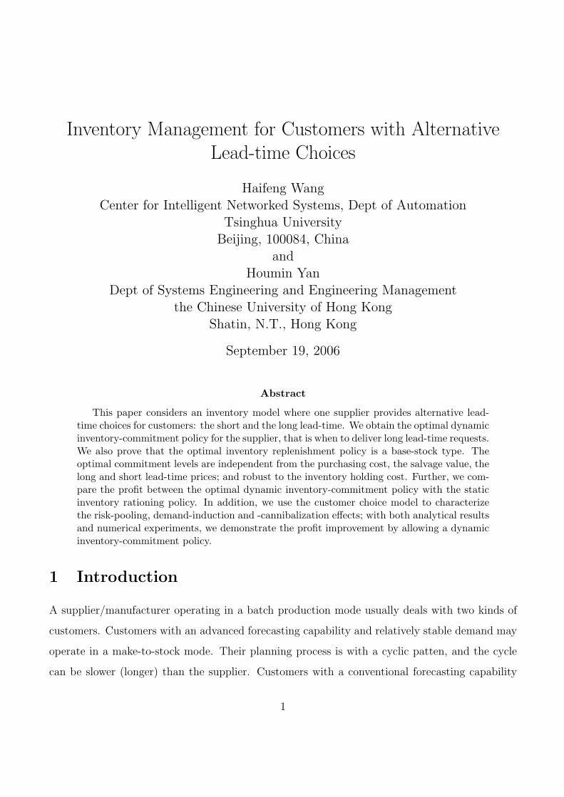
the next cycle. The sequence of events is illustrated in Figure 1.
At the beginning of each cycle, the supplier replenishes its inventory, and sets the same product
with two prices with respect to the delivery lead-time. Similar to techniques used by Gallego et
al. (2006), and Talluri and Ryzin (2004), we divide a cycle into small sub-periods {1, 2, · · · , T}.It is assumed a sub-period is small enough such that at most one customer arrives in each sub-
period. Specifically, in each sub-period, the short lead-time customer, with a probability of πs,
places an order and expects the order to be delivered immediately. Demands from these short
lead-time customers are lost if their orders cannot be satisfied immediately. With a probability
5
TTime horizon
The supplierselects a desiredinventory level
The customer chooses
The supplier promisesdelivery Schedule
delivery lead-time;
Current cyle Next cycle
In sub-period t, it comestwo types of customers:the short lead-time customer w.p. πsthe long lead-time customer w.p. πf
t1
The supplier replenishesinventory, and deliversproducts which are promisedin the previous cycle
Leftover inventoriesare slavaged
Figure 1: The Sequence of the Events and Decisions
πf , the long lead-time customer places an order and expects the order to be delivered no later
than the next cycle. The short and long lead-time customers pay a unit price ps and pf (pf ≤ ps),
respectively. Note that we assume that the supplier has a sufficient capacity, such that all long
lead-time customers can be satisfied in the next cycle. Denote also π0 as the probability of no
orders in each sub-period. Obviously, we have πs +πf +π0 = 1. At the end of each cycle, leftover
inventories are carried over to the next cycle, and a unit inventory holding cost h applies to each
unit of inventories. Leftover inventories can be salvaged at the unit price of s.
At the beginning of the next cycle, the supplier replenishes its inventory and fulfills all com-
mitted orders for long lead-time customers. In the last cycle, leftover inventories are salvaged at
the unit price of s.
To faciliate the analysis, we denote the on-hand inventory and the amount of products
promised to deliver in the next period as n(t) and m(t), respectively, where t represents the
tth sub-period of the cycle. The inventory-commitment policy for long lead-time customers at
sub-period t is
u(t) =
1, the long lead-time order to be satisfied with on-hand inventoryand delivered immediately;
0, the long lead-time order to be promised to be delivered in the next cycle.
To maximize the profit in this inventory model with alternative lead-time choices, it is neces-
sary for the supplier to find an optimal dynamic inventory-commitment policy u(t), with respect
to n(t), m(t) and the elapsed sub-period t. With an optimal inventory commitment policy, it is
possible for us to address the issue of the optimal inventory stocking, i.e. to characterize the opti-
6
mal inventory replenishment policy. The former is solved in Section 3, and the latter is discussed
in Section 4.
3 The Optimal Inventory Commitment Policy
Since the price for the short lead-time customer ps is no less than the price for the long lead-time
customer pf , it is always beneficial for the supplier to meet the short lead-time order as long as
the on-hand inventory is positive. On the other hand, it is critical to decide when to fulfill orders
from the long lead-time customers. In this section, we present a model to derive the optimal
inventory-commitment policy.
Let V (t, n, m) represent the value function from sub-period t when the amounts of the on-hand
inventory and the promised-to-delivery product are n and m, respectively. When n(t) = 0, neither
long lead-time nor short lead-time customers can be satisfied in the current period. Therefore,
the demand for the short lead-time customers is lost, and orders for long lead-time customers
are scheduled to be delivered in the next cycle. The supplier obtains a profit of pf from a long
lead-time customer, that is for 1 ≤ t < T ,
V (t, 0,m) = (π0 + πs)V (t + 1, 0,m) + πf (pf + V (t + 1, 0,m + 1)), (1)
and
V (T, 0,m) = −cm, (2)
Where c is the unit purchasing cost. With some algebraic calculations, it is possible to derive
that the value function for zero on-hand inventory is
V (t, 0,m) = (T − t)πf (pf − c)− cm. (3)
For n(t) ≥ 1, the supplier decides when the long lead-time customer can be satisfied. The
dynamic programming equation is, for 1 ≤ t < T ,
V (t, n, m) = π0V (t + 1, n, m) + πf maxu∈{0,1}
{V (t + 1, n− u,m + 1− u)}+πsV (t + 1, n− 1,m) + πfpf + πsps; (4)
7
and
V (T, n,m) = −c(m− n)+ − hn + s(n−m)+. (5)
where the unit salvage value s is assumed to be less than the unit purchasing cost c.
Remark 3.1 Although our results are derived in the discrete time setting, they can be easily
extended to a continuous time model. In this case, the value function is
V (t, n, m) = maxu
E{∫ T
t
[πsps1n(s−)>0 + πfpf1n(s−)>0u(s) + πfpf (1− u(s))]dN(s)
−hn(T )− c(m(T )− n(T ))+}= max
uλ{
∫ T
t
[πsps1n(s−)>0 + πfpf1n(s−)>0u(s) + πfpf (1− u(s))]ds
−hEn(T )− cE(m(T )− n(T ))+}, (6)
where N(t) stands for the accumulated amount of customer arrivals until time t, which is a
homogeneous Poisson process with a constant intensity λ, and s− denotes the time just before s.
Let
F (∆t) = maxu{λ∆t(πsps1n(t)>0 + πfpf1n(t)>0u(t) + πfpf (1− u(t)))
+
∫ T
t+∆t
[πsps1n(s−)>0 + πfpf1n(s−)>0u(s) + πfpf (1− u(s))]ds
−hEn(T )− cE(m(T )− n(T ))+}= max
u{λ∆t(πsps1n(t)>0 + πfpf1n(t)>0u(t) + πfpf (1− u(t)))
+V (t + ∆t, n(t + ∆t),m(t + ∆t))}, (7)
which converges to V (n,m, t), when ∆t → 0. The state transitions are n(t+∆t) = n(t)−λ∆t(πs+
πfu(t)) and m(t + ∆t) = m(t) + λ∆tπf (1− u(t)). Hence, we can obtain that, for n(t) > 0,
F (∆t) = λ∆t(πsps + πfpf ) + maxu
V (t + ∆t, n(t + ∆t),m(t + ∆t))
= λ∆t(πsps + πfpf ) + max{V (n(t)− λ∆t(πs + πf ),m(t), t + ∆t),
V (n(t)− λ∆tπs,m(t) + λ∆tπf , t + ∆t)}, (8)
which possesses a similar structure as Equation (4). Then by the same procedure of what follows in
this paper, it is easy to prove that F (∆t) preserves all of our results, for any ∆t. Let ∆t → 0, and
8
sub-period t
Dynamic Inventory CommitmentLevel Cm(t)
Deliver orders from longlead-time customersin the next cycle
Deliver orders from longlead-time customers now
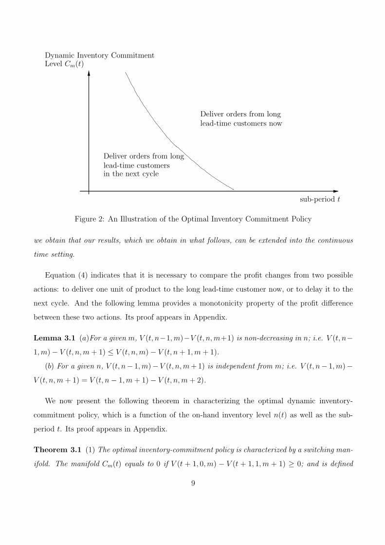
Figure 2: An Illustration of the Optimal Inventory Commitment Policy
we obtain that our results, which we obtain in what follows, can be extended into the continuous
time setting.
Equation (4) indicates that it is necessary to compare the profit changes from two possible
actions: to deliver one unit of product to the long lead-time customer now, or to delay it to the
next cycle. And the following lemma provides a monotonicity property of the profit difference
between these two actions. Its proof appears in Appendix.
Lemma 3.1 (a)For a given m, V (t, n−1,m)−V (t, n, m+1) is non-decreasing in n; i.e. V (t, n−1,m)− V (t, n, m + 1) ≤ V (t, n, m)− V (t, n + 1,m + 1).
(b) For a given n, V (t, n− 1,m)− V (t, n, m + 1) is independent from m; i.e. V (t, n− 1,m)−V (t, n, m + 1) = V (t, n− 1,m + 1)− V (t, n, m + 2).
We now present the following theorem in characterizing the optimal dynamic inventory-
commitment policy, which is a function of the on-hand inventory level n(t) as well as the sub-
period t. Its proof appears in Appendix.
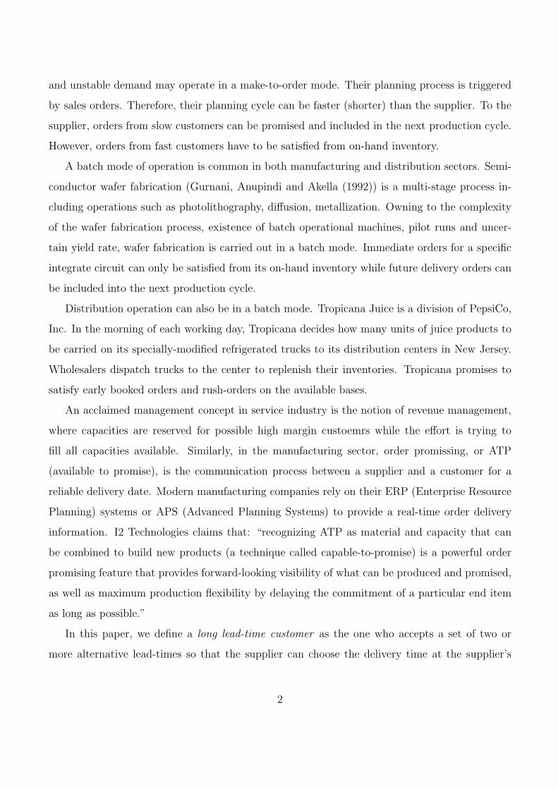
Theorem 3.1 (1) The optimal inventory-commitment policy is characterized by a switching man-
ifold. The manifold Cm(t) equals to 0 if V (t + 1, 0,m) − V (t + 1, 1,m + 1) ≥ 0; and is defined
9

as the maximum value of n such that V (t + 1, n − 1,m) − V (t + 1, n, m + 1) ≤ 0, otherwise.
Moreover, the switching manifold is independent of the next cycle promised order quantity m, and
non-increasing with respect to the time t.
(2) In each sub-period, the optimal control is: to deliver orders from long lead-time customers
now if n(t) > Cm(t); otherwise to promise long lead-time customers that their orders will be
delivered in the next cycle. The inventory-commitment policy is illustrated in Figure 2.
This theorem provides the optimal inventory-commitment policy when the supplier faces order
from a long lead-time customer. The supplier balances the trade-off between delivering products
now and delaying the orders to the next cycle: the former may save on-hand inventory to meet
potential short lead-time orders in the remaining of the cycle; the latter may reduce the on-hand
inventory to get rid of a potential inventory holding cost. The result of the trade-off is to follow
a dynamic inventory-commitment policy in Theorem 3.1.
4 The Optimal Inventory Replenishment Policy
In the last section, we have obtained the optimal inventory-commitment policy for the supplier
during the selling cycle. In this section, we extend our study to investigate the existence and the
form of the optimal inventory replenishment policy. We start from a single cycle problem.
4.1 Optimal Inventory Replenishment Policy for a Single Cycle Prob-lem
To facilitate the discussion in this section, we define V as the set of functions on f : N ×N −→ R
where N stands for {0, 1, 2, · · ·}, and if V ∈ V , then:
P1 V (t, n, m) is concave in n, for a given m;
P2 V (t, n, m) is concave in m, for a given n;
P3 V (t, n, m)−V (t, n−1,m) is non-decreasing in m, for a given n; and V (t, n, m+1)−V (t, n, m)
is non-decreasing in n, for a given m.
The following lemma claims that V (t, n, m) ∈ V . Its proof appears in Appendix.
10
Lemma 4.1 The value function V (t, n, m) ∈ V , i.e. V (t, n, m) satisfies P1, P2 and P3.
At the beginning of the selling season, the supplier has an intial inventory n(0). A desired on-hand
inventory level is selected as n(1) s.t. n(1) ≥ n(0) to maximize profits, i.e.
maxn(1)≥n(0)
(V (1, n(1), 0)− c(n(1)− n(0))) = −cn(0) + maxn(1)≥n(0)
(V (1, n(1), 0)− cn(1)),
where c(n(1)− n(0)) is the purchasing cost. This can be easily solved since V (1, n(1), 0) satisfies
the property of P1. The result can be characterized as a base-stock policy as follows.
Theorem 4.1 The inventory replenishment policy is a base-stock type, i.e. there exists an optimal
order-up-to level y∗ such that the optimal ordering quantity is
q∗ =
{y∗ − n(0), if n(0) ≤ y∗,0, if n(0) > y∗;
where y∗ is the maximizer of V (1, n(1), 0)− c(n(1)− n(0)), which is independent from n(0).
Then, with a simple search algorithm, it is possible for us to find the optimal stocking level.
4.2 Extensions to a Multi-cycle Problem
In this subsection, we extend our results into a multi-cycle problem. In the model we discussed
before, after meeting the products at the beginning of the next cycle, the left products are sal-
vaged. In the multi-cycle problem, the leftover poducts can be considered as the initial inventory
of the consequentive cycle. Then at the beginning of each cycle (except the first cycle), the inven-
tory replenishment have two functions: (1) to satisfy the orders promised in the last cycle, and
(2) to setup an initial inventory for orders in the future. Without a capacity constraint, these
two parts can be separated, because the orders promised in the last cycle are known when the
replenishment decision is made. Let i be the cycle index. For the last cycle i = I, the value
function VI(T, n,m) is the same as Equation (5). For cycle i < I, the leftover inventories are
carried over to the next cycle, and the value function can be rewritten as
Vi(T, n,m) = −c(m− n)+ − hn + maxy≥(n−m)+
{−c(y − (n−m)+) + Vi+1(1, y, 0)}= c(n−m)− hn + max
y≥(n−m)+{−cy + Vi+1(1, y, 0)}, (9)
where y is the inventory position after replenishment at the beginning of cycle i + 1. Other
dynamic equations can be carried out similarly. Now we present the following theorem.
11
Theorem 4.2 For a multi-cycle problem, the delivery policy for long lead-time customers in each
cycle is the dynamic inventory-commitment policy, characterized by Theorem 3.1.
Given the leftover inventory n and promised-to-delivery product m from the previous cycle, the
inventory replenishment at the beginning of cycle i consists of the following two parts: (1) order
(m−n)+ to satisfy the promised orders from the previous cycle; (2) order up to a base-stock level
y∗, i.e. order (y∗ − (n−m)+)+, where y∗ is the maximizer of Vi(1, y, 0)− c(y − (n−m)+).
Proof. Recall that the properties of (a) and (b) in Lemma 3.1, and P1, P2 and P3 in Lemma 4.1
are required to construct the optimal policy. It is possible for us to demonstrate that VI(T, n,m)
satisfies (a) and (b), P1, P2 and P3, and the derivative of VI(T, n, 0) with respect to n is no
greater than c. Now suppose that Vi+1(T, n,m) satisfies the above mentioned conditions. Then,
we varify if Vi(T, n,m) preserves these properties.
From the proof of Lemma 3.1 and 4.1, we obtain that Vi+1(1, n, m) satisfies (a), (b) and P1,
P2, P3. Since we have assumed that the derivative of Vi+1(T, n, 0) in n is no greater than c, by
Equation (4), it is straight forward to obtain that the derivative of Vi+1(1, n, 0) in n is no greater
than c, i.e.
Vi+1(1, n, 0)− Vi+1(1, n− 1, 0) ≤ c (10)
By the concavity of Vi+1(1, y, 0) in y (property P1), we obtain that there exists a maximizer
y∗ of −cy + Vi+1(1, y, 0), and (9) can be rewriten as
Vi(T, n,m) = c(n−m)− hn− c(y∗ ∨ (n−m)+) + Vi+1(1, y∗ ∨ (n−m)+, 0), (11)
where y∗∨ (n−m)+ equals to the maximum of y∗ and (n−m)+. From (10) and (11), it is staight
forward that the derivative of Vi(T, n, 0) in n is no greater than c.
From (11), we obtain that Vi(T, n − 1,m) − Vi(T, n,m + 1) = h, that is, Vi(T, n,m) satisfies
(a) and (b). In what follows, we prove that Vi(T, n,m) satisfies P1, P2, and P3 step by step. To
facilitate the proof, we denote
y∗ ∨ (n−m)+ =
{n−m, if n ≥ m + y∗;y∗, otherwise.
(12)
First let us fix m. When n ≥ m + y∗, then Vi(T, n,m) = c(n − m) − hn − c(n − m) +
Vi+1(1, n−m, 0) which is concave in n, since Vi+1(1, n, m) satisfies P1. The derivative of Vi(T, n,m)
12
with respect to n is no greater than −h + c by (10). When n ≤ m + y∗ − 1, Vi(T, n,m) =
c(n −m) − hn − cy∗ + Vi+1(1, y∗, 0) which is concave in n, and the derivative is −h + c. Hence
Vi(T, n,m) is concave in n, i.e. it satisfies P1.
Then let us fix n. By (10), we obtain that the derivative of Vi+1(1, n −m, 0) in m is no less
than −c. When m ≤ n − y∗, then Vi(T, n,m) = c(n −m) − hn − c(n −m) + Vi+1(1, n −m, 0)
which is concave in m, since Vi+1(1, n, m) satisfies P2. Its derivative with respect to m is no less
than −c. When m ≥ n − y∗ + 1, Vi(T, n,m) = c(n − m) − hn which is concave in m, and its
derivative is −c. Hence Vi(T, n,m) is concave in m, i.e. it satisfies P2.
When m ≤ n − y∗, then Vi(T, n,m)− Vi(T, n − 1,m) = −h + Vi+1(1, n −m, 0)− Vi+1(1, n −1 − m, 0). Vi+1(1, n − m, 0) − Vi+1(1, n − 1 − m, 0) is non-decreasing in m, since Vi+1(T, n,m)
satisfies P1. Hence, Vi(T, n,m) − Vi(T, n − 1,m) is non-decreasing in m. And it is no greater
than −h + c by (10). When m ≥ n − y∗ + 1, Vi(T, n,m) − Vi(T, n − 1,m) = −h + c. Hence
Vi(T, n,m)− Vi(T, n− 1,m) is non-decreasing in m, i.e. Vi(T, n,m) satisfies P3. To this end, we
have proved that Vi(T, n,m) satisfies P1, P2 and P3. ¤
5 Study of the Static Inventory Rationing and the Dy-
namic Inventory-Commitment Policy
In Theorem 3.1, we prove that the optimal inventory commitment policy depends on a time-
dependent switching manifold for long lead-time customers. In the literature, inventory rationing
policy assumes a constant level for different demand classes. Cattani and Souza (2002) compare
the performance of the inventory rationing policy with a first-come first-serve policy. They con-
clude that the inventory rationing policy out performs the first-come first-serve policy. In this
section, we carry out a study in comparing the performance of the dynamic inventory-commitment
policy to the static inventory rationing policy.
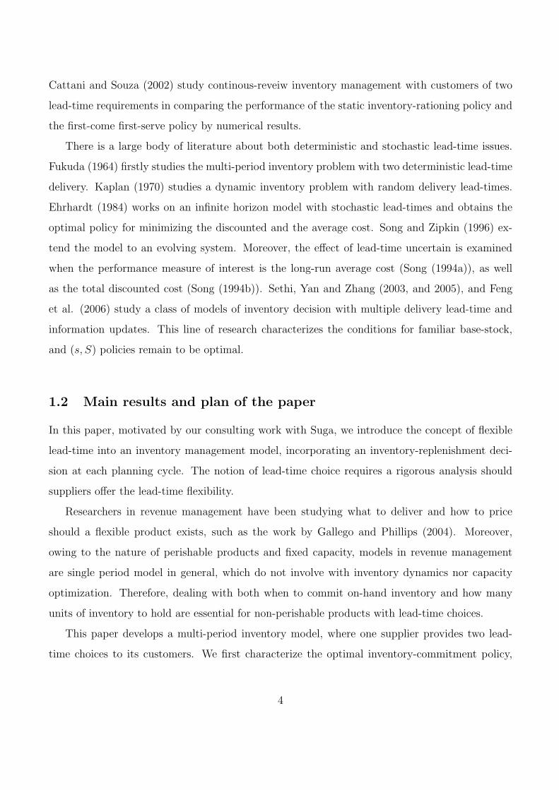
Note that for the dynamic inventory-commitment policy, according to Theorem 3.1, consists
of one optimal commitment level Cm(t) in each sub-period t, and the commitment levels vary
in different sub-periods (see Figure 3 for its illustration). The supplier delivers the long lead-
time customer a product in the current cycle as long as the inventory level is greater than the
commitment level at that sub-period. The inventory rationing policy depends on one static
13
Inventory Commitment Level Cm(t)
Deliver orders from longlead-time customers now
Deliver orders from longlead-time customersin the next cycle
Sub-period t
8
10
0 2 4 6 8 10 12 14 16
h=70
h=30
6
4
h=50
2
0
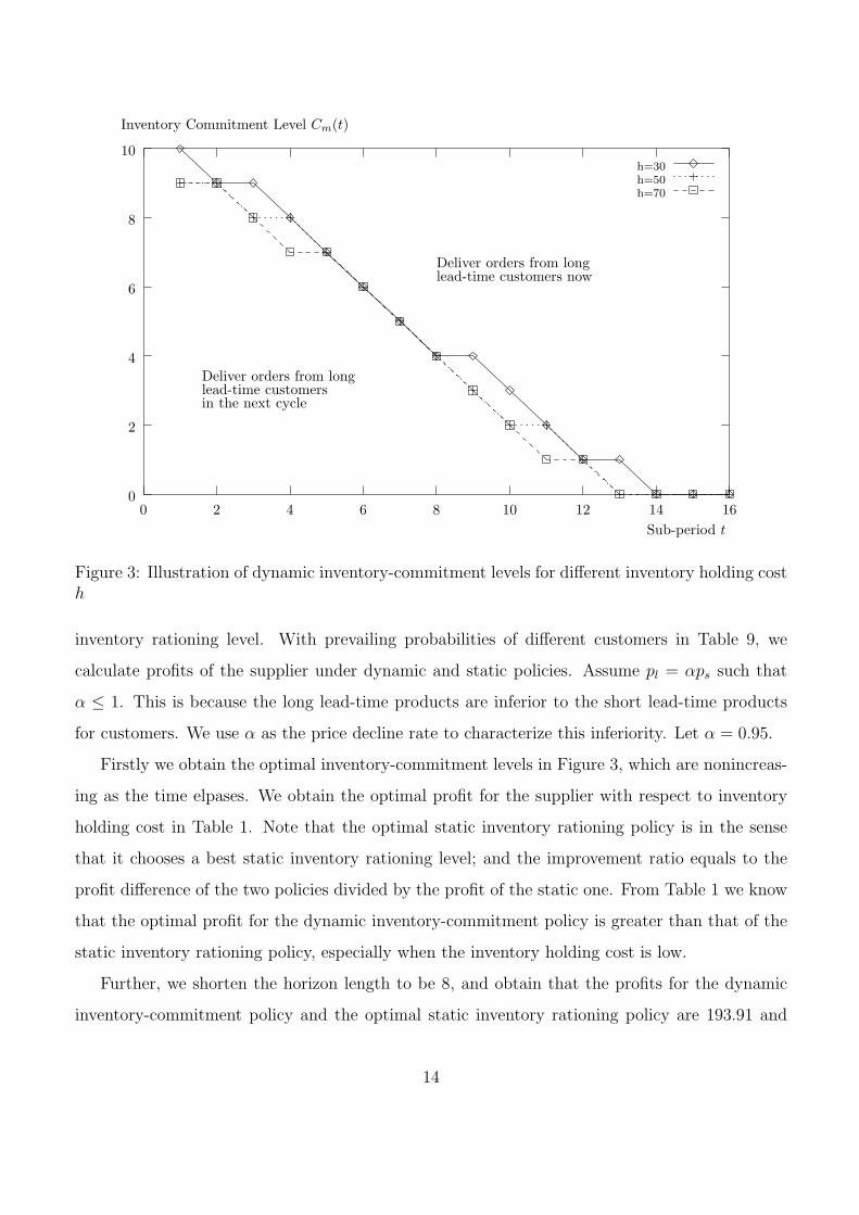
Figure 3: Illustration of dynamic inventory-commitment levels for different inventory holding costh
inventory rationing level. With prevailing probabilities of different customers in Table 9, we
calculate profits of the supplier under dynamic and static policies. Assume pl = αps such that
α ≤ 1. This is because the long lead-time products are inferior to the short lead-time products
for customers. We use α as the price decline rate to characterize this inferiority. Let α = 0.95.
Firstly we obtain the optimal inventory-commitment levels in Figure 3, which are nonincreas-
ing as the time elpases. We obtain the optimal profit for the supplier with respect to inventory
holding cost in Table 1. Note that the optimal static inventory rationing policy is in the sense
that it chooses a best static inventory rationing level; and the improvement ratio equals to the
profit difference of the two policies divided by the profit of the static one. From Table 1 we know
that the optimal profit for the dynamic inventory-commitment policy is greater than that of the
static inventory rationing policy, especially when the inventory holding cost is low.
Further, we shorten the horizon length to be 8, and obtain that the profits for the dynamic
inventory-commitment policy and the optimal static inventory rationing policy are 193.91 and
14
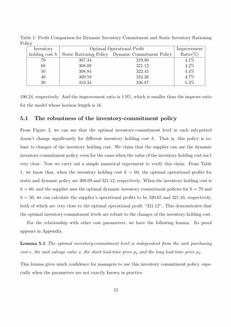
Table 1: Profit Comparison for Dynamic Inventory Commitment and Static Inventory RationingPolicy
Inventory Optimal Operational Profit Improvementholding cost h Static Rationing Policy Dynamic Commitment Policy Ratio(%)
70 307.34 319.80 4.1%60 308.09 321.12 4.2%50 308.84 322.45 4.4%40 309.59 324.26 4.7%30 310.34 326.87 5.3%
190.24, respectively. And the improvement ratio is 1.9%, which is smaller than the improve ratio
for the model whose horizon length is 16.
5.1 The robustness of the inventory-commitment policy
From Figure 3, we can see that the optimal inventory-commitment level in each sub-period
doesn’t change significantly for different inventory holding cost h. That is, this policy is ro-
bust to changes of the inventory holding cost. We claim that the supplier can use the dynamic
inventory-commitment policy, even for the cases when the value of the inventory holding cost isn’t
very clear. Now we carry out a simple numerical experiment to verify this claim. From Table
1, we know that, when the inventory holding cost h = 60, the optimal operational profits for
static and dynamic policy are 308.09 and 321.12, respectively. When the inventory holding cost is
h = 60, and the supplier uses the optimal dynamic inventory commitment policies for h = 70 and
h = 50, we can calculate the supplier’s operational profits to be 320.65 and 321.10, respectively,
both of which are very close to the optimal operational profit “321.12”. This demonstrates that
the optimal inventory-commitment levels are robust to the changes of the inventory holding cost.
For the relationship with other cost parameters, we have the following lemma. Its proof
appears in Appendix.
Lemma 5.1 The optimal inventory-commitment level is independent from the unit purchasing
cost c, the unit salvage value s, the short lead-time price ps and the long lead-time price pf .
This lemma gives much confidence for managers to use this inventory commitment policy, espe-
cially when the parameters are not exactly known in practice.
15
Sub-period t
Deliver orders from longlead-time customersin the next cycle
Deliver orders from longlead-time customers now
Inventory Commitment Levels nt
8
10
0 2 4 6 8 10 12 14 16
6
4
2
negative swing of πf
positive swing of πf
original onepositive swing of πs
negative swing of πs
0
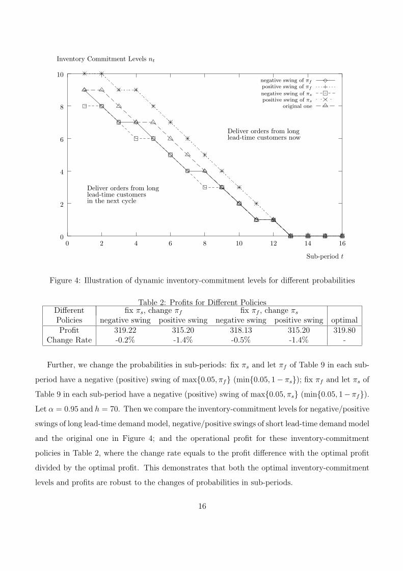
Figure 4: Illustration of dynamic inventory-commitment levels for different probabilities
Table 2: Profits for Different PoliciesDifferent fix πs, change πf fix πf , change πs
Policies negative swing positive swing negative swing positive swing optimalProfit 319.22 315.20 318.13 315.20 319.80
Change Rate -0.2% -1.4% -0.5% -1.4% -
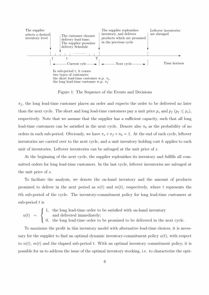
Further, we change the probabilities in sub-periods: fix πs and let πf of Table 9 in each sub-
period have a negative (positive) swing of max{0.05, πf} (min{0.05, 1− πs}); fix πf and let πs of
Table 9 in each sub-period have a negative (positive) swing of max{0.05, πs} (min{0.05, 1− πf}).Let α = 0.95 and h = 70. Then we compare the inventory-commitment levels for negative/positive
swings of long lead-time demand model, negative/positive swings of short lead-time demand model
and the original one in Figure 4; and the operational profit for these inventory-commitment
policies in Table 2, where the change rate equals to the profit difference with the optimal profit
divided by the optimal profit. This demonstrates that both the optimal inventory-commitment
levels and profits are robust to the changes of probabilities in sub-periods.
16
6 Benefit of Choice Model: Risk Pooling Effect
In order to characterize the benefits and pitfalls of providing lead-time choices to customers, in
this section, we compare models with different delivery policies. In the first model, the non-choice
model, short and long lead-time customers are satisfied by separately. In the second model, the
choice model, short and long lead-time customers are satisfied jointly, and the optimal inventory-
commitment policy, developed in Section 3 (Theorem 3.1), is deployed. In the choice model, by
pooling long lead-time customers together, the risk from demand uncertainty of short lead-time
customers is compansated. In what folllows, we develop the detailed models and use the profit
difference of these two models to demonstrate the benefits of the choice model.
In the non-choice model, short and long lead-time customers are satisfied separately by on-
hand inventory and replenished inventory of the next cycle, respectively. The leftover inventory
of the short lead-time supplier are salvaged at the end of the cycle. The long lead-time supplier
satisfies all the orders from long lead-time customers. The total profit, denoted by Vsi(n(1)), can
be written as
Vsi(n(1)) = −c ∗ n(1) + Vs(1, n(1)) + Vl, (13)
where
Vs(1, n(1)) = EDs [ps min{T∑
t=1
Ds(t), n(1)}+ (−h + s) max{n(1)−T∑
t=1
Ds(t), 0}],
Vl = (pf − c)EDl[
T∑t=1
Dl(t)]. (14)
−c ∗ n(1) is the purchasing cost at the beginning of the current cycle. Vs(1, n(1)) is the profit for
short lead-time customers, which are satisfied by the initial on-hand inventory n(1) of the current
cycle. This is similar to the traditional newsvendor model. Vl is the profit for long lead-time
customers, all of which are satisfied by the replenished inventory of the next cycle.
In the choice model, short and long lead-time customers are satisfied jointly. The profit can
be calculated by Equation (3), (4) and (5), and the optimal inventory-commitment policy and
optimal inventory replenishment policy are characterized by Theorem 3.1 and 4.1, respectively.
Since the inventory delivery policy for the non-choice model is not the optimal one, we can obtain
that the profit of the choice model is no less than the non-choice model.
17

Table 3: Probabilites of Coming Customers in Sub-periodsSub-period 1 2 3 4 5 6 7 8
π0 0.46 0.35 0.26 0.19 0.14 0.11 0.1 0.11πs = πf 0.27 0.325 0.37 0.405 0.43 0.445 0.45 0.445
Sub-period 9 10 11 12 13 14 15 16π0 0.14 0.19 0.26 0.35 0.46 0.59 0.74 0.91
πs = πf 0.43 0.405 0.37 0.325 0.27 0.205 0.13 0.045
6.1 Comparisons of two models
Assume that the unit purchasing price c is 70. The initial inventory level x = 0. The unit holding
cost h = 70 and the slavage value s = 20. One cycle includes 16 sub-periods, i.e. T = 16. In sub-
period t, assume that the probability for no customer π0(t) = (t−7)2
100+ 0.1, and the prababilities
for short and long lead-time customers are equal, i.e. πs(t) = πf (t) = 1−π0
2. Probabilities for no
customer, short and long lead-time customers are shown in Table 3. The unit price of the short
lead-time products ps is 100, and the unit price of the long lead-time products pl = αps, with
α ≤ 1. We compare profits between non-choice and choice models with a different price decline
rate α.
In order to facilitate the numerical experiment for the non-choice model, according to the
supplier’s policy in the non-choice model, we rewrite Vs(1, n(1)) in a recursive form, for n ≥ 1,
Vs(t, n) = (1− πs)Vs(t + 1, n) + πs(ps + Vs(t + 1, n− 1)), for t < T ;
Vs(T, n) = (−h + s)n. (15)
And Vs(t, 0) = 0. Then we obtain the optimal profit V ∗si = maxn(1){Vsi(n(1))} = −c ∗ n(1) +
Vs(1, n(1)) + Vl for the non-choice model. For the choice model, we use expressions (3), (4) and
(5) to calculate the optimal profit. These results are listed and compared in Table 4. Note that
the “Improvement Ratio” is the profit difference divided by the profit of the non-choice model.
Moreover, we fix the price decline rate α = 0.95, and calculate the optimal profit for different
inventory holding cost h in Table 5.
If we use the improvement ratio as an indicator for risk-pooling effect, from Table 4, it indicates
that the larger the difference in prices is, the higher the improvement ratio is, and from Table
5, it indicates that the higher the inventory holding cost is, the higher the improvement ratio is.
18

Table 4: Profits for Different Price Decline Rate, h = 70Price Decline Rate Optimal Operational Profit Improvement
α Non-choice Model Choice Model Ratio (%)1.00 245.56 292.83 19.3%0.98 234.92 282.19 20.1%0.95 218.96 264.36 20.7%0.90 192.36 239.63 24.6%0.80 139.16 186.43 34.0%
Table 5: Profits for Different Inventory Holding Cost, α = 0.95Inventory Holding Cost Optimal Operational Profit Improvement
h Non-choice Model Choice Model Ratio (%)70 218.96 266.23 21.6%60 221.23 267.73 21.0%50 223.49 269.35 20.5%40 225.76 271.09 20.1%30 228.03 273.10 19.8%
The above observation are all consist with our intuition.
6.2 Leftover inventory levels of two models
In order to further explore the risk-pooling effect, in this subsection, we use simulation to study
the leftover inventory level at the end of the current cycle n(T ). Two models start with the
same initial inventory level after ordering n(1), and experience the same demand realization. We
compare the expected value and the variance of leftover inventory levels.
Assume the price decline rate α = 0.95. We use the probabilities in Table 3 to randomly
generate 50 demand realizations. For the non-choice model, all the long lead-time customers are
backlogged and committed to deliver in the next cycle. For the choice model, the long lead-time
delivery follows the optimal inventory-commitment policy and the optimal inventory-commitment
levels are obtained by Equations (3), (4) and (5), and listed in Table 6. Then we obtain the leftover
Table 6: The Switching Curve of the Optimal Inventory Commitment Policy for α = 0.95Sub-period t 1 2 3 4 5 6 7 8
Cm(t) 7 7 6 6 5 4 4 3Sub-period 9 10 11 12 13 14 15 16
Cm(t) 2 1 1 0 0 0 0 0
19
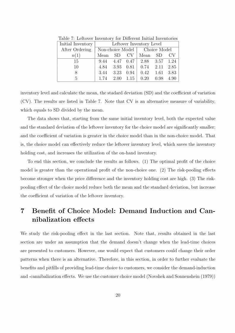
Table 7: Leftover Inventory for Different Initial InventoriesInitial Inventory Leftover Inventory LevelAfter Ordering Non-choice Model Choice Model
n(1) Mean SD CV Mean SD CV15 9.44 4.47 0.47 2.88 3.57 1.2410 4.84 3.93 0.81 0.74 2.11 2.858 3.44 3.23 0.94 0.42 1.61 3.835 1.74 2.00 1.15 0.20 0.98 4.90
inventory level and calculate the mean, the stadard deviation (SD) and the coefficient of variation
(CV). The results are listed in Table 7. Note that CV is an alternative measure of variability,
which equals to SD divided by the mean.
The data shows that, starting from the same initial inventory level, both the expected value
and the standard deviation of the leftover inventory for the choice model are significantly smaller;
and the coefficient of variation is greater in the choice model than in the non-choice model. That
is, the choice model can effectively reduce the leftover inventory level, which saves the inventory
holding cost, and increases the utilization of the on-hand inventory.
To end this section, we conclude the results as follows. (1) The optimal profit of the choice
model is greater than the operational profit of the non-choice one. (2) The risk-pooling effects
become stronger when the price difference and the inventory holding cost are high. (3) The risk-
pooling effect of the choice model reduce both the mean and the standard deviation, but increase
the coefficient of variation of the leftover inventory.
7 Benefit of Choice Model: Demand Induction and Can-
nibalization effects
We study the risk-pooling effect in the last section. Note that, results obtained in the last
section are under an assumption that the demand doesn’t change when the lead-time choices
are presented to customers. However, one would expect that customers could change their order
patterns when there is an alternative. Therefore, in this section, in order to further evaluate the
benefits and pitfills of providing lead-time choice to customers, we consider the demand-induction
and -cannibalization effects. We use the customer choice model (Novshek and Sonnenshein (1979))
20
to characterize these effects.
Specifically, we assume that the customer’s maximum willingness-to-pay (W.T.P.) for products
with current and next cycle delivery as ws and wl, respectively, where ws and wl depends on a
joint distribution over R2+ of g(ws, wl). R2
+ is a two-dimention non-negative vector. And we
assume that the maximum W.T.P. for the long lead-time delivery mode wf is a linear function of
the above two,
wf (ws, wl) = πws + (1− π)wl − ρ, (16)
where the π is the customer’s probability of receiving products at the current cycle and ρ ≥ 0 is
the premium in W.T.P. due to the delivery time uncertainty. We assume that π = 0.5 and ρ = 3.
For the non-choice model, the cusomer buys products as long as its W.T.P. is no less than the
price of the product with a short delivery lead-time, i.e. ws ≥ ps. Then the probability of the
prevailing short lead-time customers is
πs =
∫ ∞
0
∫ ∞
ps
g(ws, wl)dwsdwl. (17)
Further assume that ws and wl are independently and uniformly distributed in [0,Ws] and [0,Wl],
respectively. Then we can obtain that
πs =Ws − ps
Ws
. (18)
Let ps = 100, pf = 95 and Wl = Ws. To keep the probabilities π0 the same as in Table 3, we
set the value of Ws as in Table 8 according to Equation (18). In contract to the last section, we
demonstrate how much additional profit can be obtained after including the demand induction
and cannibalization into consideration. πs = 1− π0. In this model, all short lead-time customers
are satisfied once the supplier has positive on-hand inventory. We can use the same way as in
Equation (15) to calculate the profit in Figure 5.
For the choice model, note that probabilities are different for these customers, which is due
to demand-induction and -cannibalization effects. In what follows, we develop models for the
demand-induction and -cannibalization.
Firstly, the demand-induction is defined as an extra demand is allured by a lower selling price.
As it has been assumed, the price of the long lead-time products is no more than that of the short
21
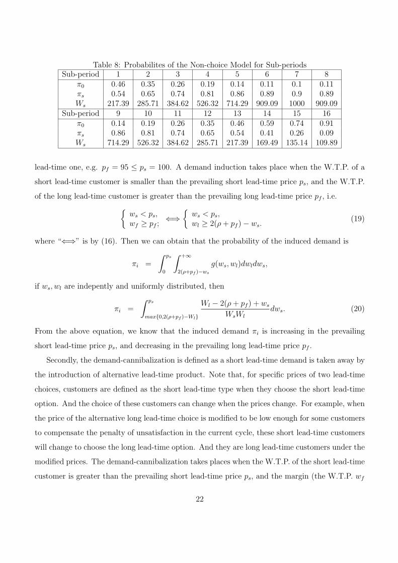
Table 8: Probabilites of the Non-choice Model for Sub-periodsSub-period 1 2 3 4 5 6 7 8
π0 0.46 0.35 0.26 0.19 0.14 0.11 0.1 0.11πs 0.54 0.65 0.74 0.81 0.86 0.89 0.9 0.89Ws 217.39 285.71 384.62 526.32 714.29 909.09 1000 909.09
Sub-period 9 10 11 12 13 14 15 16π0 0.14 0.19 0.26 0.35 0.46 0.59 0.74 0.91πs 0.86 0.81 0.74 0.65 0.54 0.41 0.26 0.09Ws 714.29 526.32 384.62 285.71 217.39 169.49 135.14 109.89
lead-time one, e.g. pf = 95 ≤ ps = 100. A demand induction takes place when the W.T.P. of a
short lead-time customer is smaller than the prevailing short lead-time price ps, and the W.T.P.
of the long lead-time customer is greater than the prevailing long lead-time price pf , i.e.
{ws < ps,wf ≥ pf ;
⇐⇒{
ws < ps,wl ≥ 2(ρ + pf )− ws.
(19)
where “⇐⇒” is by (16). Then we can obtain that the probability of the induced demand is
πi =
∫ ps
0
∫ +∞
2(ρ+pf )−ws
g(ws, wl)dwldws,
if ws, wl are indepently and uniformly distributed, then
πi =
∫ ps
max{0,2(ρ+pf )−Wl}
Wl − 2(ρ + pf ) + ws
WsWl
dws. (20)
From the above equation, we know that the induced demand πi is increasing in the prevailing
short lead-time price ps, and decreasing in the prevailing long lead-time price pf .
Secondly, the demand-cannibalization is defined as a short lead-time demand is taken away by
the introduction of alternative lead-time product. Note that, for specific prices of two lead-time
choices, customers are defined as the short lead-time type when they choose the short lead-time
option. And the choice of these customers can change when the prices change. For example, when
the price of the alternative long lead-time choice is modified to be low enough for some customers
to compensate the penalty of unsatisfaction in the current cycle, these short lead-time customers
will change to choose the long lead-time option. And they are long lead-time customers under the
modified prices. The demand-cannibalization takes places when the W.T.P. of the short lead-time
customer is greater than the prevailing short lead-time price ps, and the margin (the W.T.P. wf
22
minus the price pf ) of the long lead-time product is greater than the margin of the short lead-time
product, i.e.
{ws ≥ ps,wf − pf ≥ ws − ps;
⇐⇒{
ws ≥ ps,wl ≥ ws − 2ps + 2ρ + 2pf .
(21)
where “⇐⇒” is by (16). Then we can obtain the probability of the cannibalized demand of the
choice model is
πc =
∫ +∞
ps
∫ +∞
ws−2(ps−pf )+2ρ
g(ws, wl)dwldws,
if ws, wl are indepently and uniformly distributed, then
πc =
∫ Ws
ps
Wl − (−2ps + 2ρ + 2pf )− ws
WsWl
dws. (22)
From the above equation, we know that the cannibalized demand πc is decreasing in the prevailing
long lead-time price pf .
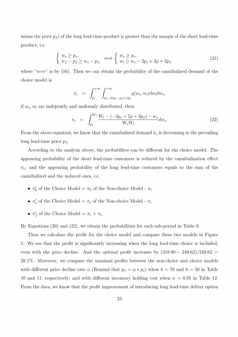
According to the analysis above, the probabilites can be different for the choice model. The
appearing probability of the short lead-time customers is reduced by the cannibalization effect
πc; and the appearing probability of the long lead-time customers equals to the sum of the
cannibalized and the induced ones, i.e.
• π′0 of the Choice Model = π0 of the Non-choice Model - πi
• π′s of the Choice Model = πs of the Non-choice Model - πc
• π′f of the Choice Model = πi + πc
By Equations (20) and (22), we obtain the probabilities for each sub-period in Table 9.
Then we calculate the profit for the choice model and compare these two models in Figure
5. We see that the profit is significantly increasing when the long lead-time choice is included,
even with the price decline. And the optimal profit increases by (319.80 − 249.62)/249.62 =
28.1%. Moreover, we compare the maximal profits between the non-choice and choice models
with different price decline rate α (Remind that pf = α ∗ ps) when h = 70 and h = 50 in Table
10 and 11, respectively; and with different inventory holding cost when α = 0.95 in Table 12.
From the data, we know that the profit improvement of introducing long lead-time deliver option
23
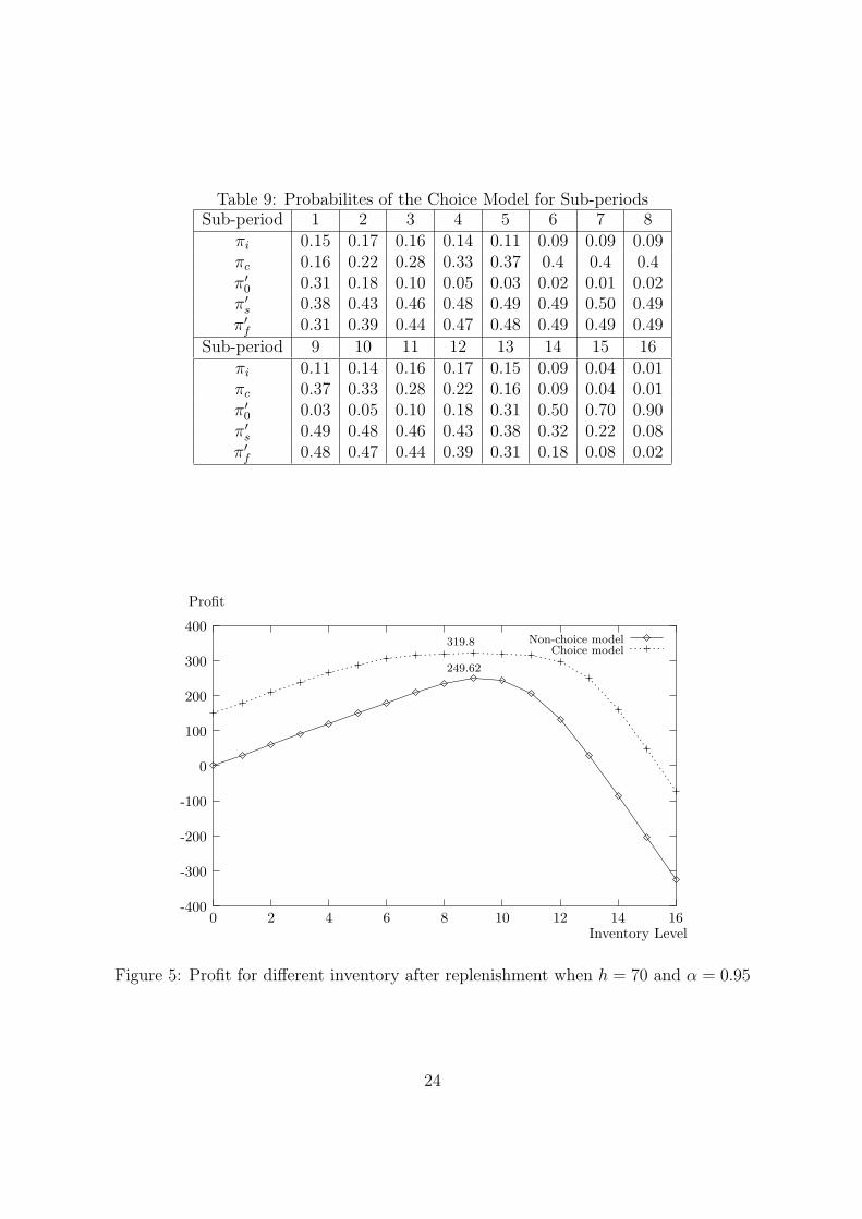
Table 9: Probabilites of the Choice Model for Sub-periodsSub-period 1 2 3 4 5 6 7 8
πi 0.15 0.17 0.16 0.14 0.11 0.09 0.09 0.09πc 0.16 0.22 0.28 0.33 0.37 0.4 0.4 0.4π′0 0.31 0.18 0.10 0.05 0.03 0.02 0.01 0.02π′s 0.38 0.43 0.46 0.48 0.49 0.49 0.50 0.49π′f 0.31 0.39 0.44 0.47 0.48 0.49 0.49 0.49
Sub-period 9 10 11 12 13 14 15 16πi 0.11 0.14 0.16 0.17 0.15 0.09 0.04 0.01πc 0.37 0.33 0.28 0.22 0.16 0.09 0.04 0.01π′0 0.03 0.05 0.10 0.18 0.31 0.50 0.70 0.90π′s 0.49 0.48 0.46 0.43 0.38 0.32 0.22 0.08π′f 0.48 0.47 0.44 0.39 0.31 0.18 0.08 0.02
Inventory Level
249.62
319.8
Profit
300Choice model
Non-choice model
1614121084 620
400
200
100
0
-100
-200
-300
-400
Figure 5: Profit for different inventory after replenishment when h = 70 and α = 0.95
24
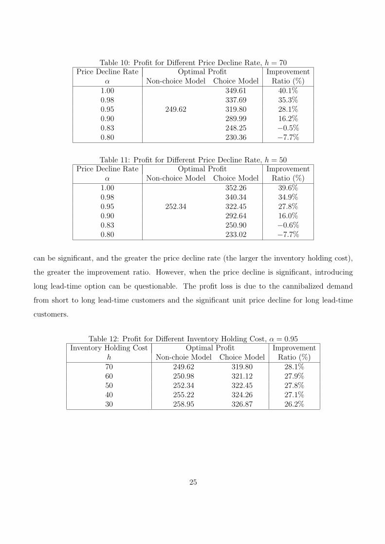
Table 10: Profit for Different Price Decline Rate, h = 70Price Decline Rate Optimal Profit Improvement
α Non-choice Model Choice Model Ratio (%)1.00 349.61 40.1%0.98 337.69 35.3%0.95 249.62 319.80 28.1%0.90 289.99 16.2%0.83 248.25 −0.5%0.80 230.36 −7.7%
Table 11: Profit for Different Price Decline Rate, h = 50Price Decline Rate Optimal Profit Improvement
α Non-choice Model Choice Model Ratio (%)1.00 352.26 39.6%0.98 340.34 34.9%0.95 252.34 322.45 27.8%0.90 292.64 16.0%0.83 250.90 −0.6%0.80 233.02 −7.7%
can be significant, and the greater the price decline rate (the larger the inventory holding cost),
the greater the improvement ratio. However, when the price decline is significant, introducing
long lead-time option can be questionable. The profit loss is due to the cannibalized demand
from short to long lead-time customers and the significant unit price decline for long lead-time
customers.
Table 12: Profit for Different Inventory Holding Cost, α = 0.95Inventory Holding Cost Optimal Profit Improvement
h Non-choie Model Choice Model Ratio (%)70 249.62 319.80 28.1%60 250.98 321.12 27.9%50 252.34 322.45 27.8%40 255.22 324.26 27.1%30 258.95 326.87 26.2%
25
8 Concluding Remarks and Further Research Direction
This paper introduces the alternative lead-time choices for the customers into the traditional fixed
and unique lead-time inventory model, and characterizes the optimal inventory replenishment
policy, as well as the optimal inventory-commitment policy within the cycle. Compared with the
production lead-time of the supplier, the lead-time choices for the customers are divided into two
catagories of the short and the long lead-time requirement: the former one asks for a delivery
lead-time which is shorter than the production lead-time of the supplier, and the latter one asks
for a delivery lead-time which is longer than the production lead-time of the supplier.
This paper demonstrates the profit improvement by including alternative lead-time choices
with both analytical results and numerical experiments. The improved profit comes from the
following sources: (1) The demand-induction effect. The lower price of the long lead-time choice
attracts the additional customers; (2) The risk-pooling effect. The long lead-time customers
provide a flexibility to the supplier in deciding when to deliver the products. The supplier
balance the trade-off between the following two things: delivering products in the next cycle to
save on-hand inventory, which meets potential short lead-time orders in the remaining cycle, and
delivering on-hand inventory now to long lead-time customers in inventory holding cost reduction.
This enables the supplier to use the future capacity together with the current capacity to satisfy
the demand. And this also enables the supplier to better control the on-hand inventory during
the selling cycle.
Our results also demonstrate that the risk-pooling effect is increasing in both the price differ-
ence of short and long lead-time customers and the inventory holding cost. The demand induction
and cannibaliztion effect is increasing in both price decline rate and the inventory holding cost.
Note that the risk pooling, demand-induction and -cannibalization effects of flexible products
in a revenue management model are investigated by Gallego and Phillips (2004). The concept
of flexible products is similar to that of the long lead-time products, because both of them let
the supplier choose from a feasible set, e.g. two feasible products or two feasible delivery lead-
times. But the concept of the long lead-time products in our paper focuses on the flexibility of
deliver time, rather than the flexibility of what to deliver. And the supplier has an opportunity of
inventory replenishment when it chooses to deliver in the next cycle. We focus on both improving
26
capacity utilization and reducing overall leftover inventory, and demonstrate that the risk-pooling
benefit of choice model comes from a reduction of the mean and the variance of leftover inventory.
The optimal inventory replenishment policy is also characterized in this paper.
Moreover, this paper compares supplier’s profit between the optimal inventory-commitment
policy and the static inventory rationing policy. Cattani and Souza (2002) compare the static
inventory rationing policy with the first-come first-serve policy and study the conditions, under
which the inventory rationing policy is beneficial. This paper demonstrates that the optimal
inventory commitment policy out-performs the static inventory rationing policy, especially when
the inventory holding cost is low and the cycle time is long. In addition, the optimal commitment
level in each sub-period is independent from the unit purchasing cost, the unit salvage cost, the
short and long lead-time prices, and robust to the inventory holding cost, so that the supplier can
achieve a “close-to-optimal” profit even when he doesn’t know these cost parameters exactly.
A very interesting issue for the future research is to introduce 3 or more lead-time choices into
the choice model: long lead-time customers require a maximume delivery time which is greater
than the production lead-time, medium lead-time customers require a maximume delivery time
which is equal to the production lead-time and the short lead-time customers require a maximume
delivery time which is shorter than the production lead-time. We need three-dimention vector
(n,m1,m2) to describe the state during the selling cycle. n stands for the on-hand inventory plus
the pipe-line inventory, m1 and m2 stand for the promised-to-deliver products in the next cycle
and in the third cycle, respectively. Study of this three lead-time choice model will shed light to
a general multiple lead-time choice model.
References
[1] Cattani, K. D. and Souza, G. C. “Inventory Rationing and Shipment Flexibility Alternatives
for Direct Market Firms”, Production and Operations Management, Vol. 11, No. 4, 441 - 457,
(2002).
[2] Chen, S. X. “The Optimality of Hedging Point Policies for Stochastic Two-Product Flexible
Manufacturing Systems”, Operations Research, Vol. 52, No. 2, 312 - 322, (2004).
27
[3] Ehrhardt, R. “(s, S) Policies for a Dynamic Inventory Model with Stochastic Leadtimes.”,
Operations Research, Vol. 32, 121 - 132, (1984).
[4] Elmaghraby, W., Lippman, S. A., Tang, C. S., Yin, R. “Pre-announced Pricing Strategies
with Reservations”, Working paper, University of Maryland, (2006).
[5] Evans, R. V. “Sales and Restocking Policies in a Single Item Inventory System”, Management
Science, Vol. 14, No. 7, 463 - 472, (1968).
[6] Feng, Q., Gallego, G., Sethi, S. P., Yan, H. and Zhang, H. “A Periodic Review Inventory
Model with Three Consecutive Modes and Forecast Updates”, Journal of Optimization The-
ory Applications, Vol. 124, No. 1, 137 - 155, (2005).
[7] Feng, Q., Gallego, G., Sethi, S. P., Yan, H. and Zhang, H. “Optimality and Nonoptimality
of Base-stock Policy in Inventory Problems with Multiple Delivery Modes”, Working paper,
University of Texas at Dallas, (2003).
[8] Fukuda, Y. “Optimal Policies for the Inventory Problem with Negotiable Leadtime”, Man-
agement Science, Vol. 10, No. 4, 690 - 708, (1964).
[9] Gallego, G., Chen, S., Lin, B. and Li, Z. “The Optimal Seat Allocation for the Two-Flight
Problems”, working paper, Columbia University, U.S.A. and Nanyang Technological Univer-
sity, Singapore. (2006).
[10] Gallego, G. and Phillips, R. “Revenue Management of Flexible Products”, Manufacturing &
Service Operations Management, Vol. 6, No. 4, 321 - 337, (2004).
[11] Gurnani, H., Anupindi, R. and Akella, R. “Control of Batch Processing Systems in Semicon-
ductor Wafer Fabrication Facilities”, IEEE Transactions on Semiconductor Manufacturing,
Vol. 5, No. 4, 319 - 328, (1992).
[12] Ha, A. Y. “Stock-rationing Policy for a Make-to-stock Production System with Two Priority
Classes and Backordering”, Naval Research Logistics, Vol. 44, 457 - 472, (1997a).
[13] Ha, A. Y. “Inventory Rationing in a Make-to-stock Production System with Several Demand
Classes and Lost Sales”, Management Science, Vol. 43, 1093 - 1103, (1997b).
28
[14] Kaplan, A. “Stock Rationing”, Management Science, Vol. 15, No. 5, 260 - 267, (1969).
[15] Kaplan, R. S. “A Dynamic Inventory Model with Stochastic Lead Times”, Management
Science, Vol. 16, No. 7, 491 - 507, (1970).
[16] Klein, M. J. and Dekker, R. “An Overview of Inventory Systems with Several Demand
Classes”, Econometric Institute Report 9839/A, Erasmus University, Rotterdam, The Nether-
lands, (1998).
[17] Mendez, C. A., Cerda, J., Grossmann, I. E., Harjunkoski, I., Fahl, M. “State-of-the-art
review of optimization methods for short-term scheduling of batch processes”, accepted by
Computer and Chemical Engineering, (2006).
[18] Novshek, W. and Sonnenschein, H. “Marginal Consumers and Neoclassical Demand Theory”,
Journal of Political Economy, Vol. 87, No. 6, 1368 - 1376, (1979).
[19] Sethi, S. P., Thompson, G. L. Optimal Control Theory: Applications to Management Science
and Economics. 2nd Ed., Kluwer Academic Publishers, 101 Philip Drive, Assinippi Park,
Norwell, Massachusetts, (2000).
[20] Sethi, S. P., Yan, H. and Zhang, H. “Peeling Layers of an Onion: Inventory Model with
Multiple Delivery Modes and Forecast Updates”, Journal of Optimization Theory and Ap-
plications, Vol. 108, No. 2, 253 - 281, (2001).
[21] Sethi, S. P., Yan, H. and Zhang, H. “Inventory Models with Fixed Costs, Forecast Updates,
and Two Delivery Modes”, Operations Research, Vol. 51, No. 2, 321 - 328, (2003).
[22] Sethi, S. P., Yan, H. and Zhang, H. “Inventory and Supply Chain Management with Forecast
Updates”, in series International Series in Operations Research & Management Science,
Springer, New York, NY, (2005).
[23] Song, J. S. “The Effect of Leadtime Uncertainty in a Simple Stochastic Inventory Model”,
Management Science, Vol. 40, No. 5, 603 - 613, (1994a).
[24] Song, J. S. “Understanding the Lead-time Effects in Stochastic Inventory Systems with
Discounted Costs”, Operations Research Letters, Vol. 15, 85 - 93, (1994b).
29
[25] Song, J. S. and Zipkin, P. “Inventory Control with Infomation About Supply Conditions”,
Management Science, Vol. 42, No. 10, 1409 - 1419, (1996).
[26] Talluri, K. T. and Ryzin, G. V. “Revenue Management Under a General Discrete Choice
Model of Consumer Behavior”, Management Science, Vol. 50, No. 1, 15 - 33, (2004).
[27] Topkis, D. M. “Optimal Ordering and Rationing Policies in a Nonstationary Dynamic In-
ventory Model with n Demand Classes”, Management Science, Vol. 15, No. 3, 160 - 176,
(1968).
[28] Veinott, A. F. Jr. “Optimal Policy in a Dynamic, Single Product, Nonstationary Inventory
Model with Several Demand Classes”, Operations Research, Vol. 13, No. 5, 761 - 778, (1965).
[29] Whittemore, A. S. and Saunders, S. C. “Optimal Inventory Under Stochastic Demand with
Two Supply Options”, SIAM J. Appl. Math., Vol. 32, No. 2, 293 - 305, (1977).
A Proof of Lemma 3.1.
It is straightforward to check that V (T, n− 1,m)− V (T, n,m + 1) = −c(m− n + 1)+− hn + h +
s(n − 1 −m)+ + c(n + 1 − n) + hn − s(n −m − 1)+ = h, which satisfies (a) and (b). Assume
that V (t + 1, n − 1,m) − V (t + 1, n, m + 1) satisfies (a) and (b). Then we need to prove that
V (t, n− 1,m)− V (t, n, m + 1) satisfies (a) and (b).
Proof of (a). After checking (4), we know that we only need to check the following inequality:
max{V (t + 1, n− 2,m), V (t + 1, n− 1,m + 1)}− max{V (t + 1, n− 1,m + 1), V (t + 1, n, m + 2)}≤ max{V (t + 1, n− 1,m), V (t + 1, n, m + 1)}− max{V (t + 1, n, m + 1), V (t + 1, n + 1,m + 2)}. (23)
We check different cases in the remaining proof.
V (t + 1, n− 2,m)−max{V (t + 1, n− 1,m + 1), V (t + 1, n, m + 2)}≤ V (t + 1, n− 2,m)− V (t + 1, n− 1,m + 1)
30
≤ V (t + 1, n− 1,m)− V (t + 1, n, m + 1)
≤ max{V (t + 1, n− 1,m), V (t + 1, n, m + 1)} − V (t + 1, n, m + 1), (24)
where the second inequality is by that V (t + 1, n− 1,m)− V (t + 1, n, m + 1) satisfies (a).
V (t + 1, n− 2,m)−max{V (t + 1, n− 1,m + 1), V (t + 1, n, m + 2)}≤ V (t + 1, n− 2,m)− V (t + 1, n− 1,m + 1)
≤ V (t + 1, n− 1,m + 1)− V (t + 1, n, m + 2)
≤ V (t + 1, n, m + 1)− V (t + 1, n + 1,m + 2)
≤ max{V (t + 1, n− 1,m), V (t + 1, n, m + 1)} − V (t + 1, n + 1,m + 2), (25)
where the second and third inequalities is by that V (t + 1, n− 1,m)− V (t + 1, n, m + 1) satisfies
(b) and (a), respectively.
V (t + 1, n− 1,m + 1)−max{V (t + 1, n− 1,m + 1), V (t + 1, n, m + 2)}≤ 0
≤ max{V (t + 1, n− 1,m), V (t + 1, n, m + 1)} − V (t + 1, n, m + 1). (26)
V (t + 1, n− 1,m + 1)−max{V (t + 1, n− 1,m + 1), V (t + 1, n, m + 2)}≤ V (t + 1, n− 1,m + 1)− V (t + 1, n, m + 2)
≤ V (t + 1, n, m + 1)− V (t + 1, n + 1,m + 2)
≤ max{V (t + 1, n− 1,m), V (t + 1, n, m + 1)} − V (t + 1, n + 1,m + 2), (27)
where the second inequality is by that V (t + 1, n− 1,m + 1)− V (t + 1, n, m + 2) satisfies (a).
Combine the above four inequalities we can obtain (23).
Proof of (b). After checking (4), we know that we only need to check the following equality:
max{V (t + 1, n− 2,m), V (t + 1, n− 1,m + 1)}− max{V (t + 1, n− 1,m + 1), V (t + 1, n, m + 2)}= max{V (t + 1, n− 2,m + 1), V (t + 1, n− 1,m + 2)}− max{V (t + 1, n− 1,m + 2), V (t + 1, n, m + 3)}. (28)
31
We check different cases in the remaining proof.
When V (t+1, n−2,m) ≥ V (t+1, n−1,m+1) and V (t+1, n−1,m+1) ≥ V (t+1, n, m+2),
by V (t + 1, n − 1,m) − V (t + 1, n, m + 1) satisfies (b) we know that V (t + 1, n − 2,m + 1) ≥V (t + 1, n− 1,m + 2) and V (t + 1, n− 1,m + 2) ≥ V (t + 1, n, m + 3). Hence (28) is equivalent to
V (t + 1, n− 2,m)− V (t + 1, n− 1,m + 1)
= V (t + 1, n− 2,m + 1)− V (t + 1, n− 1,m + 2), (29)
which is true by that V (t + 1, n− 2,m)− V (t + 1, n− 1,m + 1) satisfies (b).
When V (t+1, n−2,m) ≥ V (t+1, n−1,m+1) and V (t+1, n−1,m+1) ≤ V (t+1, n, m+2),
by V (t + 1, n − 1,m) − V (t + 1, n, m + 1) satisfies (b) we know that V (t + 1, n − 2,m + 1) ≥V (t + 1, n− 1,m + 2) and V (t + 1, n− 1,m + 2) ≤ V (t + 1, n, m + 3). Hence (28) is equivalent to
V (t + 1, n− 2,m)− V (t + 1, n, m + 2)
= V (t + 1, n− 2,m + 1)− V (t + 1, n, m + 3). (30)
Since V (t + 1, n− 2,m)− V (t + 1, n− 1,m + 1) satisfies (b), we have V (t + 1, n− 2,m)− V (t +
1, n, m+2) = V (t+1, n−2,m)−V (t+1, n−1,m+1)+V (t+1, n−1,m+1)−V (t+1, n, m+2) =
V (t + 1, n − 2,m + 1) − V (t + 1, n − 1,m + 2) + V (t + 1, n − 1,m + 2) − V (t + 1, n, m + 3) =
V (t + 1, n− 2,m + 1)− V (t + 1, n, m + 3).
When V (t+1, n−2,m) ≤ V (t+1, n−1,m+1) and V (t+1, n−1,m+1) ≥ V (t+1, n, m+2),
by V (t + 1, n − 1,m) − V (t + 1, n, m + 1) satisfies (b) we know that V (t + 1, n − 2,m + 1) ≤V (t + 1, n− 1,m + 2) and V (t + 1, n− 1,m + 2) ≥ V (t + 1, n, m + 3). Hence (28) is equivalent to
V (t + 1, n− 1,m + 1)− V (t + 1, n− 1,m + 1)
= V (t + 1, n− 1,m + 2)− V (t + 1, n− 1,m + 2), (31)
which is obviously true.
When V (t+1, n−2,m) ≤ V (t+1, n−1,m+1) and V (t+1, n−1,m+1) ≤ V (t+1, n, m+2),
by V (t + 1, n − 1,m) − V (t + 1, n, m + 1) satisfies (b) we know that V (t + 1, n − 2,m + 1) ≤V (t + 1, n− 1,m + 2) and V (t + 1, n− 1,m + 2) ≤ V (t + 1, n, m + 3). Hence (28) is equivalent to
V (t + 1, n− 1,m + 1)− V (t + 1, n, m + 2)
= V (t + 1, n− 1,m + 2)− V (t + 1, n, m + 3), (32)
32
which is true by that V (t + 1, n− 1,m + 1)− V (t + 1, n, m + 2) satisfies (b).
Combine the above four equalities we can obtain (28). ¤
B Proof of Theorem 3.1.
According to Equation (4), it is optimal to deliver now if V (t+1, n−1,m)−V (t+1, n, m+1) ≥ 0;
and optimal to deliver in the next cycle, otherwise. Lemma 3.1 provides that, for a specific sub-
period t, the value of V (t+1, n−1,m)−V (t+1, n, m+1) is non-decreasing in n and independent
from m. Hence, if V (t+1, 0,m)−V (t+1, 1,m+1) ≥ 0, then V (t+1, n−1,m)−V (t+1, n, m+1) ≥ 0
for all n ≥ 1. In this case, Cm(t) = 0 and the optimal policy is to deliver orders from long
lead-time customers now for all n ≥ 1. Otherwise, Cm(t) is the largest value of n such that
V (t + 1, n− 1,m)− V (t + 1, n, m) ≤ 0. Obviously Cm(t) is independent from m.
Following is the proof of the non-increasing property of Cm(t), with respect to sub-period t.
According to the definition of Cm(t), we know that
V (t + 1, Cm(t)− 1,m) ≤ V (t + 1, Cm(t),m + 1)
V (t + 1, Cm(t)− 2,m) ≤ V (t + 1, Cm(t)− 1,m + 1). (33)
By (4), we obtain
V (t, Cm(t)− 1,m)− V (t, Cm(t),m + 1)
= π0[V (t + 1, Cm(t)− 1,m)− V (t + 1, Cm(t),m + 1)]
+ πf [V (t + 1, Cm(t)− 1,m + 1)− V (t + 1, Cm(t),m + 2)]
+ πs[V (t + 1, Cm(t)− 2,m)− V (t + 1, Cm(t)− 1,m + 1)]. (34)
By (33) and Lemma 3.1, we have V (t+1, Cm(t)−1,m)−V (t+1, Cm(t),m+1) = V (t+1, Cm(t)−1,m+1)−V (t+1, Cm(t),m+2) ≤ 0 and V (t+1, Cm(t)− 2,m)−V (t+1, Cm(t)− 1,m+1) ≤ 0.
Hence we obtain
V (t, Cm(t)− 1,m)− V (t, Cm(t),m) ≤ 0. (35)
Since Cm(t− 1) is defined as the largest value n such that V (t, n− 1,m)− V (t, n, m) ≤ 0. Then
we obtain that Cm(t− 1) ≥ Cm(t). ¤
33
C Proof of Lemma 4.1
First of all, it is straightforward that V (T, n,m) ∈ V . Now we assume that V (t + 1, n, m) ∈ V
and prove that V (t, n, m) ∈ V . From the equation of V (t, n, m), we know that we only need to
focus on the part of max{V (t + 1, n− 1,m), V (t + 1, n, m + 1)}. In the following we prove that
T (n,m) := max{V (t + 1, n− 1,m), V (t + 1, n, m + 1)}
satisfies P1, P2, P3 step by step.
Proof of P1. By Lemma 3.1, we know that given m, there exists a Cm(t)(m) such that for
n ≤ Cm(t), T (n,m) = V (t + 1, n, m + 1) is concave in n; and for n ≥ Cm(t) + 1, T (n,m) =
V (t + 1, n− 1,m) is concave in n. We now only need to obtain the following inequalities to prove
the concavity of T (n,m) in n: (In the following of the part Proof of P1, without confusion we
use T (n) instead of T (n,m) for notation simplification)
T (Cm(t) + 2)− T (Cm(t) + 1) ≤ T (Cm(t) + 1)− T (Cm(t)) (36)
T (Cm(t) + 1)− T (Cm(t)) ≤ T (Cm(t))− T (Cm(t)− 1) (37)
or equivalently,
V (t + 1, nt + 1,m)− V (t + 1, Cm(t),m) ≤ V (t + 1, Cm(t),m)− V (t + 1, Cm(t),m + 1) (38)
V (t + 1, Cm(t),m)− V (t + 1, Cm(t),m + 1) ≤ V (t + 1, Cm(t),m + 1)− V (t + 1, Cm(t)− 1,m + 1).
(39)
We have
V (t + 1, Cm(t),m + 1) ≥ V (t + 1, Cm(t)− 1,m) (40)
V (t + 1, Cm(t),m) ≥ V (t + 1, Cm(t) + 1,m + 1) (41)
Then we can obtain that
V (t + 1, Cm(t),m)− V (t + 1, Cm(t),m + 1)
≤ V (t + 1, Cm(t),m)− V (t + 1, Cm(t)− 1,m)
≤ V (t + 1, Cm(t),m + 1)− V (t + 1, Cm(t)− 1,m + 1), (42)
34
where the first inequality is by (40), and the second one is by P3 of V (t + 1, Cm(t),m). Hence we
obtain (39).
We also can obtain that
V (t + 1, Cm(t),m)− V (t + 1, Cm(t),m + 1)
≥ V (t + 1, Cm(t) + 1,m + 1)− V (t + 1, Cm(t),m + 1)
≥ V (t + 1, nt+1 + 1,m)− V (t + 1, Cm(t),m), (43)
where the first inequality is by (41) and the second one is by P3 of V (t + 1, Cm(t) + 1,m). Hence
we obtain (38).
Proof of P2. By Lemma 3.1, we know that given n, there exists a mt+1(n) such that for m ≤mt+1, T (n,m) = V (t+1, n, m+1) is concave in m; and for m ≥ mt+1, T (n,m) = V (t+1, n−1,m)
is concave in m. We now only need to obtain the following inequalities to prove the concavity of
T (n,m) in m: (In the following of the part Proof of P2, without confusion we use T (m) instead
of T (n,m) for notation simplification)
T (mt+1 + 2)− T (mt+1 + 1) ≤ T (mt+1 + 1)− T (mt+1) (44)
T (mt+1 + 1)− T (mt+1) ≤ T (mt+1)− T (mt+1 − 1) (45)
or equivalently,
V (t + 1, n− 1,mt+1 + 2)− V (t + 1, n− 1,mt+1 + 1)
≤ V (t + 1, n− 1,mt+1 + 1)− V (t + 1, n, mt+1 + 1); (46)
V (t + 1, n− 1,mt+1 + 1)− V (t + 1, n, mt+1 + 1)
≤ V (t + 1, n, mt+1 + 1)− V (t + 1, n, mt+1). (47)
We have
V (t + 1, n− 1,mt+1 + 1) ≥ V (t + 1, n, mt+1 + 2) (48)
V (t + 1, n− 1,mt+1) ≤ V (t + 1, n, mt+1 + 1) (49)
Then we can obtain that
V (t + 1, n, mt+1 + 1)− V (t + 1, n, mt+1)
35
≥ V (t + 1, n− 1,mt+1)− V (t + 1, n, mt+1)
≥ V (t + 1, n− 1,mt+1 + 1)− V (t + 1, n, mt+1 + 1), (50)
where the first inequality is by (49), and the second one is by P3 of V (t + 1, n, mt+1 + 1). Hence
we obtain (47).
We also can obtain that
V (t + 1, n− 1,mt+1 + 1)− V (t + 1, n, mt+1 + 1)
≥ V (t + 1, n, mt+1 + 2)− V (t + 1, n, mt+1 + 1)
≥ V (t + 1, n− 1,mt+1 + 2)− V (t + 1, n− 1,mt+1 + 1), (51)
where the first inequality is by (48) and the second one is by P3 of V (t + 1, n, mt+1 + 2). Hence
we obtain (46).
Proof of P3. Similarly, by equation (4), we only need to show that T (n,m) satisfies P3, i.e.
max{V (t + 1, n− 1,m), V (t + 1, n, m + 1)}− max{V (t + 1, n− 2,m), V (t + 1, n− 1,m− 1)}≤ max{V (t + 1, n− 1,m + 1), V (t + 1, n, m + 2)}− max{V (t + 1, n− 2,m + 1), V (t + 1, n− 1,m + 2)} (52)
In the following, we check different cases.
V (t + 1, n− 1,m)−max{V (t + 1, n− 2,m), V (t + 1, n− 1,m + 1)}≤ V (t + 1, n− 1,m)− V (t + 1, n− 2,m)
≤ V (t + 1, n− 1,m + 1)− V (t + 1, n− 2,m + 1)
≤ max{V (t + 1, n− 1,m + 1), V (t + 1, n, m + 2)} − V (t + 1, n− 2,m + 1), (53)
where the second inequality is by P3 of V (t + 1, n, m).
V (t + 1, n− 1,m)−max{V (t + 1, n− 2,m), V (t + 1, n− 1,m + 1)}≤ V (t + 1, n− 1,m)− V (t + 1, n− 1,m + 1)
≤ V (t + 1, n− 1,m + 1)− V (t + 1, n− 1,m + 2)
≤ max{V (t + 1, n− 1,m + 1), V (t + 1, n, m + 2)} − V (t + 1, n− 1,m + 2), (54)
36
where the second inequality is by P2 of V (t + 1, n− 1,m).
V (t + 1, n, m + 1)−max{V (t + 1, n− 2,m), V (t + 1, n− 1,m + 1)}≤ V (t + 1, n, m + 1)− V (t + 1, n− 1,m + 1)
≤ V (t + 1, n, m + 2)− V (t + 1, n− 1,m + 2)
≤ max{V (t + 1, n− 1,m + 1), V (t + 1, n, m + 2)} − V (t + 1, n− 1,m + 2), (55)
where the second inequality is by P3 of V (t + 1, n, m).
V (t + 1, n, m + 1)−max{V (t + 1, n− 2,m), V (t + 1, n− 1,m + 1)}≤ V (t + 1, n, m + 1)− V (t + 1, n− 1,m + 1)
≤ V (t + 1, n− 1,m + 1)− V (t + 1, n− 2,m + 1)
≤ max{V (t + 1, n− 1,m + 1), V (t + 1, n, m + 2)} − V (t + 1, n− 2,m + 1), (56)
where the second inequality is by P1 of V (t + 1, n, m). And combine the above 4 inequalities we
obtain the inequality (52). ¤
D Proof of Lemma 5.1
It is straightforward to check that V (T, n− 1,m)− V (T, n,m + 1) = −c(m− n + 1)+− hn + h +
s(n− 1−m)+ + c(n + 1− n) + hn− s(n−m− 1)+ = h, which is independent from c, s, ps and
pf . Assume that V (t + 1, n− 1,m)− V (t + 1, n, m + 1) is independent from c, s, ps and pf . Then
we need to prove that V (t, n− 1,m)− V (t, n, m + 1) is independent from c, s, ps and pf .
After checking (4), we know that we only need to check
max{V (t + 1, n− 2,m), V (t + 1, n− 1,m + 1)}−max{V (t + 1, n− 1,m + 1), V (t + 1, n, m + 2)} (57)
is independent from ps and pf . We check different cases in the remaining proof.
When V (t+1, n−2,m) ≥ V (t+1, n−1,m+1) and V (t+1, n−1,m+1) ≥ V (t+1, n, m+2),
Equation (57) is equivalent to V (t + 1, n − 2,m) − V (t + 1, n − 1,m + 1), which is independent
from c, s, ps and pf .
37
When V (t+1, n−2,m) ≥ V (t+1, n−1,m+1) and V (t+1, n−1,m+1) ≤ V (t+1, n, m+2),
Equation (57) is equivalent to V (t+1, n−2,m)−V (t+1, n, m+2) = [V (t+1, n−2,m)−V (t+1, n−1,m+1)]+[V (t+1, n−1,m+1)−V (t+1, n, m+2)]. Since V (t+1, n−2,m)−V (t+1, n−1,m+1)
and V (t+1, n−1,m+1)−V (t+1, n, m+2) are all independent from c, s, ps and pf , then Equation
(57) is independent from c, s, ps and pf .
When V (t+1, n−2,m) ≤ V (t+1, n−1,m+1) and V (t+1, n−1,m+1) ≥ V (t+1, n, m+2),
Equation (57) is equivalent to 0, which is independent from c, s, ps and pf .
When V (t+1, n−2,m) ≤ V (t+1, n−1,m+1) and V (t+1, n−1,m+1) ≤ V (t+1, n, m+2),
Equation (57) is equivalent to V (t + 1, n− 1,m)− V (t + 1, n, m + 1), which is independent from
c, s, ps and pf . ¤
38