Z Symbolic Computation (1991) 11,455-469

Invariant and Geometric Aspects of Algebraic Complexity Theory I

JACQUES M O R G E N S T E R N

University of Nice & LN.R.LA., Pare Valrose, F-O6034-Nice, France

(Received 17 April 1989)

We expound new approaches to the analysis of algebraic complexity based on synthetic and algebraic geometry. The search for interesting lower bounds is a good reason to study the complexity of computation of linear forms. The analysis of linear algorithms leads naturally to questions about computational networks with their combinatorial aspects and about special configurations of sets of points in projective spaces which classical invadant theory might help to answer.

Introduction

This work aims at making a bridge between old subjects: the theory of invariants o f Gln(K), algebraic geometry, and more recent ones: computat ional networks and the complexity of computat ion.

This paper should help to understand properties of sets computable in a given number , m, of basic operations and the conditions they must satisfy, for which very little is known, in general, due to the combinatorial explosion of the number of configurations leading to the same complexity. A subsequent paper will provide answers to some questions in projective geometry arising f rom our statement of the basic problems of algebraic complexity theory.

In order to motivate readers f rom different areas such as synthetic geometry, com- binatorics and invariants, computat ional complexi ty (algebraic and general), we shall t ry in section 1 to recall a few definitions and facts which will be developed and used in subsequent sections.

1. Algebraic Complexity from the Point of View of Lower Bounds

I f we are permitted to use one of the four basic arithmetic operations: +, - , * , / , we can compute any rational expression of finitely many variables x l , x2,. �9 �9 x, over any given ground field K. We shall often assume K =/~, w h e r e / ~ is the algebraic closure:

EXAMPLE 1.

f = (XlX2 + X3)/(X2 + X4)

can be computed using h~ = x~ * x2, h2 = ht + x3, h3 = x2+ x4, h4 = h2/h3 = f

DEFINITION 1.1 (Borodin & Munro, 1975). More generally a rational algorithm of length m is a sequence of rational fractions: {h~}-,~i<_m where

h i = x - i f o r i < 0 , h o = l

0747-7171/91/050455 + 15 $03.00/0 �9 1991 Academic Press Limited

456 J. Morgenstern

and

hi=hjohk for i>--1 andj, k<i or hicK

The set B = K u { x a . . . . . x~} is the base of the algorithm and o is one of the four arithmetical operations.

Lower bounds on the number of those arithmetical steps which are necessary to obtain some family of fractions are not easy to obtain. Tools have been developed based primarily on algebraic independence or dimension of linear manifolds (PAN's method; see Winograd, 1970), degree of algebraic varieties (STRASSEN's method; see Strassen, 1973) or other more specific approaches.

Among the different functions to be computed, bilinear forms have been intensively studied because of the unsolved problem of the complexity of matrix multiplication. The complexi ty o f even simpler functions, namely linear forms, has been analysed, and the following fact is now well known: any method which provides a lower bound in terms of additions for the computat ion of sets of linear forms will give a lower bound for the complexity o f computat ion of any set of rational functions: if one differentiates the given algorithm step after step, one obtains an algorithm which computes the differentials (as linear forms) of that set at some point with the same overall complexity (Morgenstern, 1971; Strassen, 1976). This, together with the impact of the Fast Fourier Transform algorithm (Cooley & Tukey, 1965), justified the interest in studying the complexity of computa t ion of l inear forms, and more specifically their additive complexity. We are going to examine three different models of computat ion which are useful for our analysis: Linear Forms; DAGs (Directed Acyclic Graphs) of Computation; and Algebraic and Synthetic Geometry.

1.1. LINEAR FORMS AND LINEAR ALGORITHMS

DEFINITION 1.2. Let K be a field and let xl , x2, . . . , x, be the coordinates forms on K". A sequence h = {h~}i . . . . ~,,Q of linear forms is a linear algorithm of basis x~ . . . . , x, if

h~=x_; f o r i < 0 , (1)

h~=A~hp+tz~hq for i>O,p,q<i,A~ and/z~ being in K ;

i f A~ and tz~ are in K* , it is an effective addition.

The first n elements of the sequence corresponding to negative indices are always the same (the coordinate forms).

I f v = {vl, v 2 , . . . , vt} is a family of t given linear forms, h computes v if v c h.

EXAMPLE 2. I f

Vt = x~ +2x2+3x3

v2 = 2x~ +3x2 + 6x3

then h_3=xa , h_2=x2, h_l=Xl, hl=h_l+3h_3, hz--'hl+2h-2, ha=2hl+3h-2 and we have v~ = h2 and v2 = h3 which are thus computed in three steps.

Algebraic ComplexityTheory 457

( o )

f g

h 2 = v~ h 3 = v 2 (b)

x I x 2 X~

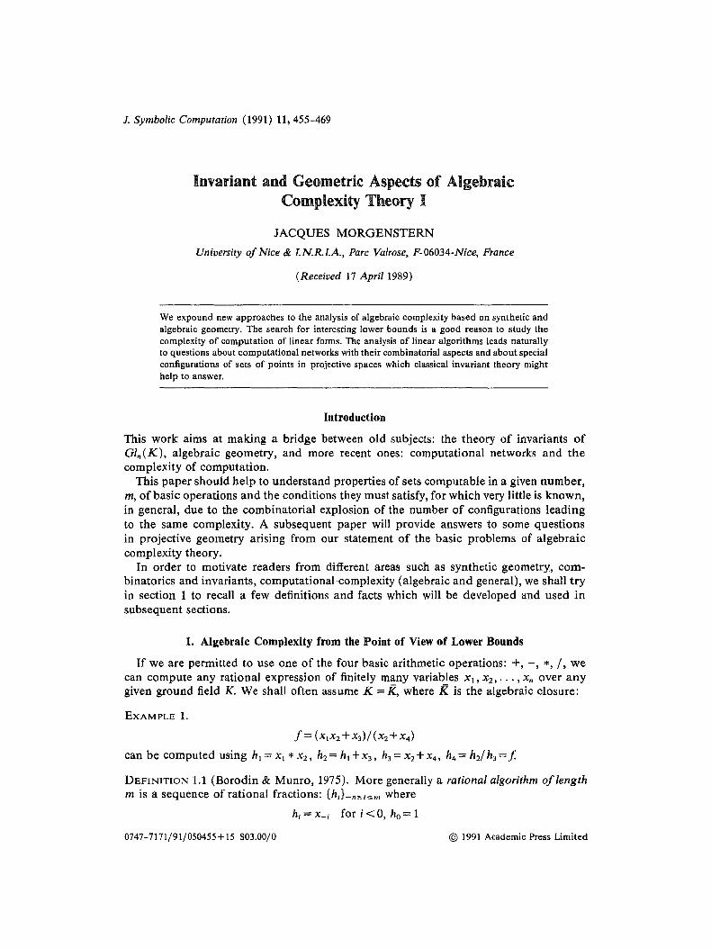
Figure 1. (a) General step, hf+l, zg and (b) Example 2.

One can find many examples in Morgenstern (1978).

1.2. C O M P U T A T I O N A L D A G S ; G E N E R A L C O M P L E X I T Y

Linear algorithms are equally well represented by directed acyclic graphs with n input nodes (in-degree 0) and such that each other node has a fan-in (in-degree) of exactly 2, finite fan-out (out-degree) and stands for a linear combination o f the two forms a l ready computed at the two ancestor nodes: ~,g+l.*h; A a n d / z will be the scalar labels of the corresponding two edges. At the t output nodes (no fan-out) linear forms are computed .

FACT: the coefficient o f x~ in vk is the sum of the product of the scalar labels on the different paths from x~ to vk.

To each linear algorithm corresponds one specific DAG. To each DAG correspond up to topological sorting a family of algorithms with different parameters.

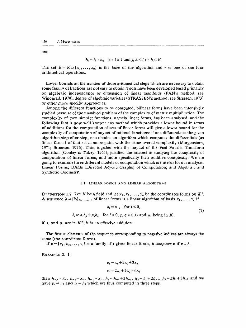
When there are internal nodes with out-degree 1, we could allow any finite fan-in according to the Figure 2 t ransformation scheme.

In general the number of additive operations is given by:

L+(DAG) = e - v + n

where e is the number of edges in the DAG, v is the number o f vertices in the D A G , and n is the number of input vertices in the DAG.

Moreover, there are in general many different DAGs corresponding to the computa t ion of the same set of linear forms with the same number of additions.

h h

h I h 2 h 3 h 4 h, h 2 h 3 h 4

Figure 2. Standard transformation,

458 J. Morgenstern

In Kaminski , Kirkpatrick & Bshouty (1988) the model is used to give an elegant proof of the fact tha t the complexity of computing the linear forms Ax where A is a t x n matrix over K is equal to the complexity of computing ('~A)y, plus n - t. Just reverse the direction o f the arrows in the DAG: this is a special case of geometric duality.

As shown in Figure 3, the first graph computes ( U, V, W) from (X, Y, Z, T); the second graph does the reverse. The Boolean analog to our problem is the following: Given a set X = { x , , . . . , x ,} of n elements, given a family v of t subsets of X, and using union as our on ly operat ion we try to reach the family v from the n elements of X. The question then: "is the family computable in less than r operat ions?" is NP-complete (as is its Boolean equivalent with disjunctions) see Garey & Johnson (1979). On the other hand we know f rom Garey & Johnson (1979) as a consequence of the "Exact Cover Problem" that given s vectors in K" , to decide if v could be computed from them in less than r addit ions is an NP-complete problem for K = Q or any finite field. Therefore, to determine the general additive complexity of a given set of forms is hard. Its analysis nevertheless sheds some more light on complexity classes of algebraic computations (Garey & Johnson, 1979).

1.3. THE GEOMETRICAL MODEL

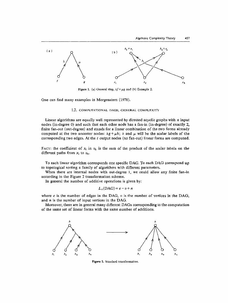
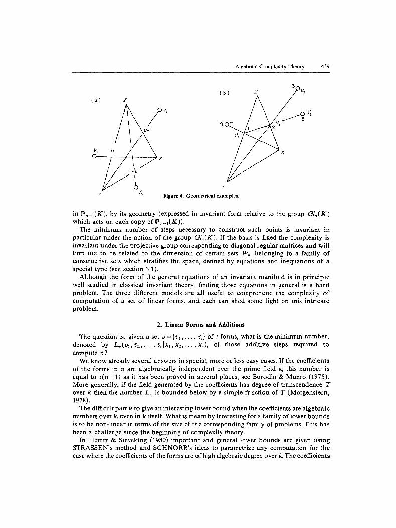
Let V. be the dual vector space of K " of dimension n on K; thus V. is the space of linear forms on K". I f we consider the corresponding projective linear space P , - I ( K ) of dimension n - 1 over K, each point can stand for a family of linear forms in the given variables. To the coordinate forms x l , . . . , x , , correspond X1 . . . . . X , a basis of P ,_ I (K) . Since we are interested in additions we identify two forms that are proportional . The geometrical counterpar t o f the additive combination is the following basic construction: given two already constructed distinct points G and H in that space, choose a point F on the line through them, F e (G, H) , and add it to the set. So, our problem becomes: given a set o f n points X 1 , . . . , X , forming a basis of P ,_1(K) , how many basic construct ion steps are required to reach a given family of t other points ?

EXAMPLE 3 (see Figure 4). Here X, Y, Z, is the basis, 1:1, V2 and V3 are to be constructed. In Figure 4(a) six addit ions are needed; in Figure 4(b), five are sufficient because U~, U3, V2 lay on the same line.

If we notice now that algorithms are not affected by a regular change of coordinates, we see that the situation is completely defined by the relative positions of the n + t points

(o ) u V w (b) X Y Z T

X Y Z T C/ V Ir

Figure 3. (a) Eight additions = 1 6 - 1 2 + 4, (b) Seven additions = 14 -10 + 3.

Algebraic Complexity Theory 459

(a) Z

r v~

/ ~b) z /~v~

Figure 4. Geometrical examples,

in P ,_~(K) , by its geometry (expressed in invariant form relative to the group G I , ( K ) which acts on each copy of P , - I ( K ) ) .

The minimum number of steps necessary to construct such points is invariant in particular under the action of the group GI, (K) . If the basis is fixed the complexity is invariant under the projective group corresponding to diagonal regular matrices and will turn out to be related to the dimension of certain sets W,, belonging to a family o f constructive sets which stratifies the space, defined by equations and inequations o f a special type (see section 3.1).

Although the form of the general equations of an invariant manifold is in principle well studied in classical invariant theory, finding those equations in general is a hard problem. The three different models are all useful to comprehend the complexity o f computation of a set o f linear forms, and each can shed some light on this intricate problem.

2. Linear Forms and Additions

The question is: given a set v = { v l , . . . , v,} of t forms, what is the minimum number, denoted by L + ( v l , v 2 , . . . , v , lx l ,x~ . . . . . x,), of those additive steps required to compute v ?

We know already several answers in special, more or less easy cases. If the coefficients of the forms in v are algebraically independent over the prime field k, this number is equal to t(n - 1) as it has been proved in several places, see Borodin & Munro (1975). More generally, if the field generated by the coefficients has degree of transcendence T over k then the number L+ is bounded below by a simple function of T (Morgenstern, 1978).

The difficult part is to give an interesting lower bound when the coefficients are algebraic numbers over k, even in k itself. What is meant by interesting for a family of lower bounds is to be non-linear in terms of the size of the corresponding family of problems. This has been a challenge since the beginning of complexity theory.

In Heintz & Sieveking (1980) important and general tower bounds are given using STRASSEN's method and SCHNORR's ideas to parametrize any computation for the case where the coefficients of the forms are of high algebraic degree over k. The coefficients

460 J. Morgenstern

of the target family v are seen as images by a polynomial application of the parameters o f the computa t ion with estimation of dimension and degrees. To the author 's knowledge the only o the r result along those lines is in Morgenstern (1973) where the size of a de te rminan t over C plays the central role.

I f we consider the matrix 7/" of the coefficients of the family v of t given forms, obvious l inear dependencies between subrows of ~ lead to certain savings and are measured by the null i ty o f certain determinants as seen in the example above: more generally if a form vr in n variables is a l inear combinat ion of r - 1--< n other forms vl, v2, . . . , vr_a and if we c o m p u t e v as Eh~-v i for j going from 1 to r - 1 , we can compute the whole family in

(r - 1)(n - 1) + r - 2 additions, saving (*)

n - 1 - ( r - 2 ) = n - r + 1 additions over the standard algorithm. (**)

In the case r =2 , this has been proved to be the only possible savings of additions (Kirkpatr ick , 1972).

It has been falsely conjectured (by the author for instance!) that if all the subdeter- minants of ~ are different f rom zero (let us call this the A-property), then the complexity would be necessari ly non-linear. This has been disproved by Strassen, through the analysis o f certain D A G s called superconcentrators (see Valiant, 1977). These computat ional DAGs have the proper ty tha t f rom each set o f m inputs (the variables) and m outputs (the forms to be computed) for 1-< m-< n, there are m disjoint paths connecting them. Now, if we set the scalar labels A of the edges all equal to 1 on the different paths and 0 elsewhere, the corresponding subdeterminant is a permuta t ion determinant. Therefore its value is +1 or - 1 so that the corresponding symbolic determinant with all the As is not zero.

Such families of superconcentrators have been built with a number of edges and nodes linear in the size n of the inputs by Pippenger (1978) implying thus a simple linear complexity. The matr ix W of finite Fourier t ransform has the A-property for instance when its o rder is pr ime (see Dieudonn6 (1970) and Morgenstern (1978)). This interplay be tween D A G s and l inear forms leads us to the following analysis.

3. Directed Acyelic Graph and Additions

Consider the incidence matrix D of an ari thmetic D A G 9 ; namely an m by m matrix where m is the total number of nodes of the DAG and whose coefficient D~ is the scalar labelling the edge f rom the ith to the j th node of ~ or 0. Up to permutat ion D is an uppe r t r iangular matrix with 0s on the diagonal and having other combinator ial properties. Now it is a simple fact to establish that the powers D k of D are matrices whose coefficients (Dk);~ are the sums of the products o f the labels on the paths of length exactly k from the node i to the node j. F rom the fact of section 1.2, we deduce that the coefficient ofx~ in the linear form computed at node j is equal to the i, jth coefficient of the sum ED k, k = 0 , . . . , depth (~) .

Therefore , if we are given a set 'Y of t linear forms with a corresponding matrix V in n variables, a computat ional D A G ~ of depth d computes ~ iff there exist a tr iangular matrix B having ls on the diagonal whose last t columns and first n rows is the matrix V and such that ( I - D) -~ = B, since D is a nilpotent matrix and D o = I = Identity. For instance does there exist an incidence matrix D of a graph of depth d less than log n such tha t ( I - D) -1 contains the matrix of the Discrete Fourier Transform in the upper-right corner?

Algebraic Complexity Theory 461

4. Geometries: Synthetic and Algebraic

As stated in the Introduct ion the geometrical construction corresponding to a l inear algorithm is the following: to the coordinate forms xj correspond points {Xj}j~t~.n I forming a base X of the projective space P , - I ( K ) .

As we shall be interested in varieties defined in certain product spaces [ P , _ I ( K ) ] m, if we have a set V of t points V1, V 2 , . . . , Vt to reach, we shall be dealing with the space [P._,(K)] "+'.

The construction corresponding to (1) would be a finite sequence of points in P ,_I ( K ) . H = { . . . H _ I , H ~ , . . . , H , . . . , He} such that

Hi = X_i i f i < 0

Hi e ( H , , Hq) if i > 0 and p, q < i (linear dependency) (2)

H is of length m, and computes V if V c H. The question is: what is the length o f a shortest sequence H containing the set V of given points ? What are the algebraic propert ies of such a sequence H ? The t points will be a special configuration over an infinite field if m < t (n - 1).

4.2. CAYLEY (OR GRASSMANN) ALGEBRAS

Let V be an n dimensional space over K (see Rota, 1976; White, 1990). Assume tha t a multilinear alternate form [X1, X 2 , . . . , X~] called the "bracket" is defined on V; the bracket can be defined as the determinant if a basis is given. On the product space (V) p with p <- n define the following equivalence relation:

( X , , X 2 , . . . , Xp) ~- (I,'1, V 2 , . . . , II , ) iff 3(Z~ . . . . , Z , _ , ) s.t.

[X1, Xz . . . . , X v , Z , , Z2, . . . , Z , _ v] =[I I1 , Y2, . . . , Y , , Z1, Z2, . . . , Z ,_v] .

DEFINITION 4.1 (see Rota, 1976; White, 1990). The quotient of (V) p by this equivalence relation are the extensors o f step p.

We shall denote them by X1 v X2 v . . �9 v Xp (this is simply a way to define the p t h exterior o f V). On the set of all the extensors the jo in product v compatible with the previous equivalence relation is therefore defined. The support ( A ) of an extensor A ~ 0 is the vector space generated by any set of components.

PROPERTIES 4.2.

(A) = (B) -~ ~X e KA = AB

A v B # 0~-> (A) c~ (B) = 0; in that case (A) + (B) = (A v B)

There is a dual operat ion that can be defined on extensors. Let A = (a~, a2, . . . , ak) and B = (b~, b = , . . . , bin) be two sequences of vectors of V..

DEFINITION 4.3 (Rota, 1976; Sturmfels & White, 1988). The meet product A ^ B is defined by either

A ^ B = O i f k + m < n o r k > n o r m > n

or

A ^ B = ~ ' ( -1 )~[a~(1) . . . a,~( , -m)bl . . , bm]a,~(,-m+l)v. . , va~(k)

where the summation ~" is taken over all permutations cr such that o r ( l )< �9 �9 < c r ( n - m) and t r ( n - r e + l ) < ' �9 �9 < or(k) (it is called an " n - m , k shuffle" product).

462 J. Morgenstern

PROPERTIES 4.4. A A B = (--1)t"-k)("-m)B A A; A' A B' = A A B i fA and A', B and B' define the same extensors, A A B r 0 iff (A)+ (B) = V and in that case its support (A A B) = (A) c~ (B). The meet A is associative.

DEFINITION 4 . 5 . The set of extensors on V with the two operations join and meet is a

Cayley Algebra.

It is known that any incidence relation among subspaces of V or P ,_a (K) can be written using the Cayley algebra (Doubilet, Rota & Stein, 1974; Sturmfels & White, 1988). Another approach is the general setting of Bourbaki "Bi-g~bres et Co-g~bres" Alg~bre III. Linear dependence is retained in the Cayley Algebra on V underlying P,,_a(K). If we use the convent ion above, and note the join product by v, we could rephrase (2) if

H. e Hq. H . v Hq v H, = O p. q < i, else t-I, = H . = t4.. (3)

This in turn can be written

V Y1 . . . V Y,-3 [Hp, Hq, Hi, Y ~ , . . . , Y,-3] = 0 if Hp ~ Hq else Hi = Hp = Hq (4)

where the n - 3 points can be taken among the base X and the bracket corresponds to the n by n determinant. Now, it is a well established fact (Rota, 1971) that those determinants are not independent; among them we have the basic relations called the syzygies, a term which was first used exactly for the ideal generated by the following polynomials:

(i) [ V~, Va, V 3 , . . . , V,] (a bracket with repeated entries) (ii) [V~.(l~, V~(2~,..., V~(,)]

- s ign(cr) [Vl . . . . , V,] for any permutat ion cr on [1, n] (iii) [ U ~ , . . . , U~][V~,..., V.]

- ~ j [ u , , . . . , u . _ , , Vjl[V, . . . . . yj_,, u . , y~+, . . . . . v . ]

(5)

for any possible points Us and Vs of P ,_~(K). They are properties of the determinants and consequences of the C R A M E R relations. The second fundamental theorem ofinvariant theory (Doubilet , Rota & Stein, 1974; Rota, 1971) states that there are no other algebraic relations than the ones generated by those equalities (5).

4.2. ALGEBRAIC GEOMETRY POINT OF VIEW

Consider now the tensor product algebra over K, 1-Ii of homogeneous polynomials in nt variables Y~j, i= 1 , . . . , t ; j = 1 , . . . , n,

I I , = K [ Y n , Y~2, . . . , Y ~ , , ] | Y 2 , ] | . | . . . . , Y,,].

II~ is homogeneous separately in the t families of indeterminates and any closed set o f [P,_~] ' ( for the Zariski 's topology) is defined by equations that are homogeneous separately in the t sets of variables (see Shafarevitch, 1977), and we have projective dimension: dimK I I t = (n -- 1)t.

Algebraic Complexity Theory 463

PROPOSITION 4.6. Consider the ideal I in P3 generated by either the 3• 3 minors corresponding to (3) or the n • n determinants corresponding to (4), and taking (5) inIo account, one has:

cod imK(I I3 / I ) = 2 n + 1 , or dimK(Yi3/I) = n - 2 ;

compare with (*) & (**) of section 2.

PROOF. (See Northcott (1976) for the case K = / ~ or Bruns & Vetter (1988) for the general case.) Let us see another useful argument. Consider more generally r x r determinants of an r • n matrix, r-< n, L the ideal generated; if we denote each minor by the indices of the columns: [1, 2 . . . . . r] being the first one f rom the left, then [1, 2 , . . . , r - 1, r + 1] etc. we see that up to the minor [1, 2 , . . . , r - l , n] they form a regular sequence in the corresponding algebra Hr defined by the nr variables in r rows, since each one depends on new variables. Let I ' be the ideal generated by those minors, any other determinant is a zero divisor in the quotient algebra Ylr/I ' in view of 5(iii). Therefore codim~c ( I I J I ) = cod im r ( I I J I ' ) = r(n - 1) - (n - r + 1) = n ( r - 1) - 1 (compare with (*)).

REMARK. The quantified condit ion (4) could then be reduced for instance to the conjunc- t ion of the corresponding n - 2 independent conditions: if the Xs form a basis of ~ ,,_ 1 ( / ( ) .

[ Hp, Hq, H,, X4, . . . , X , ] = [ Hp, Hq, H,, X3 , Xs , . . . , X,, ]

= [Hp, Hq, H,, Xa, X 4 , . . . , X ,_ ,] = 0. (6)

To each additive constructive step corresponds a set o f such n - 2 polynomial equations.

DEFINITION 4.7. An ideal o f Hm+n generated by the family of polynomials Y,7 with i # j , i ~ n, j-< n corresponding to the 0 coefficient of the coordinates forms xj of the basis, and the polynomials associated with the conditions (6) is an algorithmic ideal or A, , - ideal of IIn+m.

The notat ion can be simplified by identifying Ylm+n with Hm instead, the X~ being fixed (0 . . . . , 1 , . . . , 0), the restriction o f an A-ideal will be also called an Am-ideal o f II , , and will correspond to the conditions (6).

PROPOSITION 4.8. Let ~ = IIh,jll e [ P , _ I ( K ) ] m be the class o f the m by n matrix of the coe~cients of linear forms h, i f h is a linear algorithm of length m then ~ belongs to some zero set o f an Am.ideal.

PROOF. This is obvious f rom the definition since it is just the algebraic translation of the existence of such a l inear algorithm.

PROPOSITION 4.9. For an algorithm of length m, the m ( n - 2 ) polynomials corresponding to (6) form a regular sequence in the algebra l'Im.

PROOF. In fact, as in Proposition 4.6, each new equation involves a new indeterminate and therefore the corresponding term is not a zero divisor in the quotient algebra of the algebra of the polynomials in all the variables divided by the ideal previously generated, and are in complete intersection.

,164 J. Morgenstern

PROPOSITION 4.10. l f .~ iS an A-ideal in the algebra i-I,. corresponding to an algorithm of length m then

codim(II,"/~r = m -- m(n - 1) - m ( n - 2 ) . (7)

DEFINITION 4.11. Cons ider the family 1,. o f all the A-ideals corresponding to algorithms o f length m (or to computat ional DAGs with m non-leaf nodes) and let W,. be the cor responding zero algebraic set in [ P . _ I ( K ) ] tN], where [N] denotes finite subsets of N; these sets are the m-sets. Each of their points can be seen as a two-dimensional array.

We want to know what is the set Ct,,,, of t forms computable in less than m additions. To each computat ional D A G (or algorithm) Gt, computing t forms, corresponds the set C,,,.,~ (resp. C~,.,o) of all the t forms that could be computed using this DAG in --<m (resp. exactly m) additions.

PROPERTY 4.12. If at each step the three forms are distinct then C~ is an open (and constructible) connected smooth set of [P ._ I (K) ] t. Its closure is therefore an irreducible variety.

PROOF. Just look at the parameters of the computation, the As, and move them a bit! The sets C,~ o f t forms computable in m additions are finite (but huge!) unions o f such

0 C t, , . , G .

PROPOSITION 4.13, Let V be a family of t points of P._l(resp. v a family of r linear forms in n variables). They are constructible (resp. computable) in less than m steps only i f their corresponding matrix V of coefficients belongs to the projection qrt on [P . -a ] ' of the algebraic set defined in [P._l ] 'n as some m-set. (Here ~rt selects the t copies of P . - I ( K ) corresponding to V..)

PROOF. I f there is such an algorithm, it is a sequence of length m of points in P , - I ( K ) ; we can consider the corresponding matrix of the coefficients in [P , - I (K) ] , . . These coefficients satisfy a certain family of equations of the given type above, i.e., they belong to an m-set defined by an Am-Ideal. Conversely any projection of a point in such an m-set on [P ,_~(K)] ~ does not unfortunately correspond to r points constructible in m steps (the case Hi ~ Hp = Hq for instance is possible) (compare with Strassen, 1973).

4.3. E L I M I N A T I O N AND EQUATIONS

The corresponding algebraic problem is in fact an elimination problem in Cayley Algebra.

EXAMPLE (Morgenstern, 1978). Take three linear forms in four variables:

U = a . X + b . Y + c . Z + d . T;

V = a ' . X + b ' . Y + c ' . Z + d ' . T;

W = a " . X + b " . Y + c " . Z + d " . T.

I f the fol lowing equation is satisfied one addition can be saved:

( b" a - a"b )( a ' b" - a"b')( c d ' - c'd)

= ( a b ' - a ' b ) ( a ' b " - a"b ' )cd"- c"d ' (ab ' - a'b)(b"a - a"b) + c"d"(ab'- a'b) 2

Algebraic Complexity Theory 465

The geometrical situation in P3(K) is the following: U, V, W, $1, $2, $3 are on the same plane, $1, $2 and W are on the same line (see Figure 5).

Therefore if S3=3~Z+(~T, then S ~ = a S X + b S Y + ( c ~ - d y ) Z and S 2 = a ' y X + b ' yY+(yd ' - c ' 8 )T . When W, $1, $2 are on a same line, the condition depends on the proportionality of the coefficients of two linear equations in y, 8:

(c"(ab'- a'b) + c(a'b"- a"b'))t3 - d(a 'b"- a"b')y = O,

(c'(ab"- a"b)8 + (d"(ab'- ha') - d'(ab"- a"b)y = O,

which lead to the above condition:

(b"a - a"b)(a'b"- a"b')(cd'- c'd)

= (ab ' - a'b)(a'b"- a"b')cd"- c"d'(ab' - a'b)(b"a - a"b) + c"d"(ab'- a'b) 2,

which in turn could be written:

( b" a - a"b )( a 'b"- a"b')( c d ' - c'd )

= (ab ' - a'b){{(a'b"- a"b')c+(ab'- a'b)c"}d"- (ab"- a"b)c"d'},

Expressing everything within the brackets one can get (a determinant being created in the { } adding and subtracting (ab"-a"b)c'):

[Z, T, U, W][Z, T, V, W][X, Y, U, V] = [Z, T, U, V][T, U, V, W][X, Y,Z, W]

+[Z, T, U, V][X, Y, V, W][Z, 7", U, W], (8)

for the previous situation with U, V, W depending on X, Y, Z, T we have

1 X v Y v H a = 0 2 H ~ v Z v S I = O 3 Y v T v H 2 = O 4 H 2 v X v S 2 = O 5 Z v T v S 3 = O 6 S a v S 2 v W = O 7 S l v S 3 v U = 0 8 S 2 v S 3 v V = 0 .

If we eliminate H1 a n d / / 2 between 1 & 2, 3 & 4 we get: [X, II, Z, $1] = 0, [X, Y, T, $2] = 0 then $3 in 5 & 7, 8: [$1, U, Z, T] = 0, [$2, V, Z, T] = 0.

Y z H,(M) ~ S , ( 2 )

)r"

Figure $. A 3-dimensional special configuration. The order of each operation from 1 to 8 instead ot"9 is indicated in parentheses.

466 J. Morgenstern

Using just concatenation for the join, we could also write:

$3 = UVW ^ ZT; SI = X Y Z A S3U; S2= X Y T ^ S3 V

and then using "the shuffle product" we get:

S~ = [ ZUVW] T - [ TUVW]Z

S~ = [ XYZS3] U - [ XYZU] $3 = [ XYZT] [ ZUVW] U

- [XYZU][ZUVW] T + [XYZU][ TUVW]Z

S2 = [XYTS3] V - [XYTV]S3 = [XYZT][ UVWT] V

- [XYTV][ UVWZ] T+ [XYTV][ UVWT]Z.

Since for any point W over Z, T, U, V one could write:

W = [ WTUV]Z + [ZWUV] T+ [ZTWV] U+ [ZTUW] V.

The condi t ion of colinearity of $1, $2, W is on the components of U, V, Z for instance:

[ X Y Z T ] [ ZUVW] [ XYZT] [ UVWT] [ WTUV]

+ [XYZU][ TUVW] [XYZT] [ UVWT][ZTWV]

-- [ XYZT] [ ZUVW] [ XYTV] [ UVWT] [ ZTUW]

-----0,

which simplifies to

[ X Y Z T ] [ZUVW] [ WTUV]

+ [ X Y Z U ] [ TUVW] [ZTWV] - [ZUVW] [XYTV] [ZTUW]

-----0,

The under l ined term is the fixed basis, but we do not replace it by 1 yet. Fixing the order X, Y, Z, T, U, V, W the three summands are: (1): ( [XYZT][ZUVW])[TUVW] where the parenthesis can be expanded using the

syzygy 5(iii):

[ XZUV] [ YZTW] + [ YZUV] [XZTW] + [ZTUV] [XYZW],

(2): - ( [XYZU][TUV.W])[ZTVW] where the same expansion gives

+ [ Y Z U V ] [ X r U W ] + [ x z u v 3 [ V T U W ] - [XVUV][ZTUW],

(3): -([XYTV][ZUVI,~V])[ZTUW] gives rise to

- [ x z u v ] [ Y T V W ] - [ Y Z U V 3 [ X T V W ] + [ZTUV][XYVW].

The bold face terms together with their third bracket factor gives back the relation (8). The other sums are 0 since they are both symmetric and antisymmetric with respect to the permutat ion of X and Y.

Algebraic Complexi ty Theory 467

4.4. THE DUAL PROBLEM

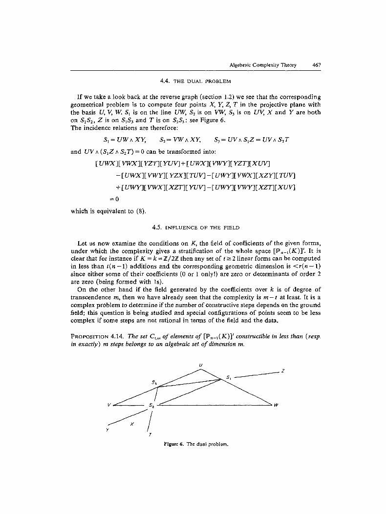
I f we take a look back at the reverse graph (section 1.2) we see that the corresponding geometrical problem is to compute four points X, Y, Z, T in the projective plane with the basis U, V, W. S~ is on the line UW, $2 is on V-W, $3 is on UV, X and Y are bo th on S~$2, Z is on $1S3 and T is on $2S3: see Figure 6. The incidence relations are therefore:

$1 = UW ^ X Y , $2 = VW ^ XY, $3 = UV ^ S1Z = UV ^ $2 T

and UV A (S~Z A S2T) = 0 can be transformed into:

[ UWX][ VWX][ YZT][ YUV] + [ UWX][ VWY][ YZT][XUV]

- [ UWX][ VWY][ YZX][ TUV] - [ UWY][ VWX][XZY][ TUV]

+ [ UWY][ VW-X][XZT] [ YUV] - [ UWY]I" VWY][XZT][XUV]

= 0

which is equivalent to (8).

4.5 . I N F L U E N C E OF THE FIELD

Let us now examine the conditions on K, the field of coefficients of the given forms, under which the complexity gives a stratification of the whole space [P ,_ I (K) ] ' . I t is clear that for instance if K = k = Z / 2 Z then any set of t - 2 linear forms can be computed in less than t ( n - 1 ) additions and the corresponding geometric dimension is < r ( n - 1) since either some of their coefficients (0 or 1 only!) are zero or determinants of order 2 are zero (being formed with Is).

On the other hand if the field generated by the coefficients over k is of degree of transcendence rn, then we have already seen that the complexity is m - t at least. It is a complex problem to determine if the number o f constructive steps depends on the ground field; this question is being studied and special configurations o f points seem to be less complex if some steps are not rational in terms of the field and the data.

PROPOSITION 4.14. The set Ct, m of elements of [ P . - I ( K ) ] ' constructible in less than (resp. in exactly) rn steps belongs to an algebraic set o f dimension m.

U

V W

T

Figure 6. The dual problem.

468 J. Morgenstern

PROOF. Corollary of Proposition 4.13 since projection preserves inclusion and decreases dimension.

4.6. CLASSICAL INVARIANT THEORY

PROPERTrES 4.15. We know that the C,.,,, are invariant under the following transforma- tions.

Action of the group Gln (K) (acting on [P,_I(K)] t+" including the basis) since the Ws have invariant significance.

Action of the Torus (,~t, h 2 , . . . , Xn), hj ~ 0 for all j, acting on [P,_1(K)]'.

From the first fundamental theorem of invariant theory and GRAM's theorem (Rota, 1971) we know that the defining equations of such varieties can be taken in the following form.

They are homogeneous with respect to the rows and columns of the matrix of the coefficients of the t points and homogeneous with respect to the brackets constructed on the n + t vectors (including the basis). If we go back to our previous example:

U = a . X + b . Y + c . Z + d . T

V = a ' . X + b ' . Y + c ' . Z + d ' . T

W = a " . X + b " . Y+c" . Z + d " . T,

the equation:

(b"a - a"b)(a'b"- a"b')(cd'- c'd)

= ( a b ' - a 'b)(a 'b"- a"b')cd"- c"d'(ab'- a'b)(b"a - a"b) + c"d"(ab'- a'b) 2

was transformed into

[ z, T, U, W]E Z, L K W][ X, Y, U, V] =[Z, T, U, V]ET, U, V, W][X, Y;,Z, W]+[Z, T, U, V][X, Y, V, W][Z, T, U, W]

which has the required properties: homogeneous in the brackets; homogeneous with respect to the vectors; and homogeneous with respect also to the columns of the underlying matrix.

Of course it is not true that any equation of this type is a useful equation to save additions! It is therefore an interesting problem to decide which ones are.

5. Further Research

Our project is therefore to design an automatic elimination process in Cayley Algebras to find the equations and inequations with invariant significance that could help determine to which constructible set Wa (in the sense of algebraic geometry) a given set of forms might belong (or not belong). The following questions may be asked.

(i) Is the set of t points reachable in m operations closed? The answer is no. (ii) Is there always a minimal algorithm to reach t points which is rational with respect

to the input points? (iii) What is a good algorithm for elimination in Cayley Algebras? (iv) What is a good description of the set of special configurations? Describe the

stratification. (v) What is true for any field? What is not?

Algebraic Complexity Theory 469

T h e s e q u e s t i o n s wi l l be d i s c u s s e d in a n o t h e r p a p e r , f o l l o w i n g s u g g e s t i o n s o f

A. H i r s c h o w i t z and B. S tu rmfe l s , w h o m I t h a n k fo r the i r h e l p as wel l as L. B a r a t c h a r t ,

N . W h i t e a n d t h e r e fe rees .

References

Borodin, A., Munro, I. (1975). The Computational Complexity of Algebraic and Numerical Problems. New York: Elsevier.

Bruns, W., Vetter, U. (1988). Determinantal rings. Lecture Notes in Mathematics 1327. Heidelberg: Springer. Cooley, J. M., Tukey, J. W. (1965). An algorithm for the machine calculation of complex Fourier series. Math.

Comput. 19, 297-302. Dieudonne, J. A. (1970). Une propd6t6 des racines de l'unit6. Revista de la Union Matematica Argentina 25. Doubilet, P., Rota, G. C., Stein, J. (1974). Foundations of combinatodcs IX: Foundations of combinatorial

methods in invariant theory. Study Appl. Math. 53, 185-216. Garey, M. R., Johnson, D. S. (1979). Computability and Intractability. New York: Freeman. Heintz, J., Sieveking, M. (1980). Lower bounds for polynomials with algebralc coefficients. Theoretical Computer

Science 11, 321-330. Kaminski, M., Kirkpatrick, D., Bshouty, N. (1988). Addition requirements for matrix and transposed matrix

products. J. Algorithms 9, 354-372. Kirkpatrick, D. G. (1972). On the number of additions necessary to compute certain functions. In: Proceedings

of the 4th A C M Syrup. on Theory of Computing pp. 94-99. Morgenstern, J. (1971). On Linear Algorithms in Theory of Machines and Computations. New York: Academic

Press. pp. 59-66. Morgenstern, J. (1973a). Algorithmes lin6aires tangents et complexit6. Compte Rendu de I'Acad~mie des Sciences

277, 367-370. Morgenstern, J. (1973b). Note on a lower bound of the linear complexity of the Fast Fourier Transform. J.

Assoc. Comput. Maeh. 20, 305-309. Morgenstern, J. (1978). Compexit6 lin6aire de Calcul. Th6se d'Etat du 27 Novembre 1978, Universit6 de Nice. Northcott, D. G. (1976). Finite Free Resolution. Cambridge: Cambridge University Press. Pippenger, N. (1978). Superconcentrators. SIAM J. Computing 6~ 298-304. Rota, G. C. (1976). Th6orie combinatoire des invariants classiques 1976. Sgries de Mathdmatiques Pures et

Appliqu~es. Strasbourg: IRMA. Rota, G. C. (1971). Combinatorial Theory and Inuariant Theory. Bowdoin College, Maine. Shafarevitch, I. R. (1977). Algebraic Geometry. Heidelberg: Springer. Strassen, V. (1976). Vermeidung yon Divisionen. 3". Reine Ange. Math. 264. Strassen, V. (1973). Die berechnungskomplexit~it von elementarsymmetrisctien funktionen. Numerische

Mathematik 20, 238-251. Sturrafels, B., White, W. (1988). Symbolic computations in geometry. IMA Preprint series 389. University of

Minnesota. Valiant, L. G. (1977). Graph theoretic arguments in low-level complexity. Lecture Notes in Computer Science $3. White, N. (1990). Multilinear Cayley factorization. J. Symbolic Computation 11, 421-438. Winograd, S. (1970). On the number of mutliplieations necessary to compute certain functions. Communication

on Pure and Applied Mathematics 23.