intrusion detection system for electronic …...\intrusion detection system for electronic...
TRANSCRIPT

“Intrusion Detection System for Electronic Communication Buses:A New Approach”
Matthew Spicer
Thesis submitted to the Faculty of theVirginia Polytechnic Institute and State University
in partial fulfillment of the requirements for the degree of
Masters of Sciencein
Mechanical Engineering
Alfred L. Wicks, ChairAmos L. Abbott
Steve C. Southward
December 11, 2017Blacksburg, Virginia
Keywords: CAN bus, Machine learning, Frequency analysis, WaveletsCopyright 2017, Matthew Spicer

“Intrusion Detection System for Electronic Communication Buses: A NewApproach”
Matthew Spicer
Academic Abstract
With technology and computers becoming more and more sophisticated and readily avail-able, cars have followed suit by integrating more and more microcontrollers to handle tasksranging from controlling the radio to the brakes and steering. Handling all of these sepa-rate processors is a communication system and protocol known as Controller Area Network(CAN) bus. While the CAN bus is a robust system for sending messages, allowing control ofthe car through the CAN bus presents an opportunity for an outside party to interfere withthe operations of a car. Any number of different methods could be used to hack the bus andtake control of a car, including hacking into the bus remotely, plugging a small device intothe on-board diagnostics port to the CAN bus, or swapping an existing node on the CAN busfor one that has been tampered with. This presents obvious safety risks, so to guard againstthis possibility, this paper will present an algorithm designed to recognize nodes based onthe noise content of their signal so that any messages coming from an improper source canbe flagged as suspicious.
The algorithm makes use of MATLAB R© and Python to perform various transformationson the data and calculate features of the noise in a signal. These features are then passedthrough a statistical analysis which provides each one a score for how much useful informa-tion it contains. The best performing features are run through both a multilayer perceptronneural network and a support vector machine, and the results are compared. Each algorithmgives strong prediction performance, with prediction accuracies of 99.9% and 99.8% for theneural network and support vector machine, respectively.
“Intrusion Detection System for Electronic Communication Buses: A NewApproach”
Matthew Spicer
General Audience Abstract
With technology and computers becoming more and more sophisticated and readily avail-able, cars have followed suit by integrating more and more microcontrollers to handle tasksranging from controlling the radio to the brakes. Handling all of these separate processors isa communication system and protocol known as Controller Area Network (CAN) bus. How-ever, this presents an opportunity for an outside party to interfere with the operations of acar. An existing node for the CAN bus could be swapped out for one that has been tamperedwith, causing potentially fatal accidents. To guard against this possibility, this paper willpresent an algorithm designed to recognize nodes based on the noise content of their signalso that any new hardware will trigger a flag that an unrecognized source is trying to inter-fere. The algorithm makes use of the MATLAB R© and Python programming languages tocalculate certain characteristics of the noise in the signal and pass those through a machinelearning algorithm. This algorithm is able to learn through mathematical means what eachnode ”sounds like”. With over 99% accuracy, we were able to predict which node sent agiven signal.

Acknowledgments
I would like to thank Dr. Wicks for all of his guidance during my my time with the Mecha-tronics Lab. Not only did he help me with this project, but he allowed me a great opportunityto explore many different subject areas that I was previously unfamiliar with and find some-thing that I really enjoyed doing. I would like to thank each of my committee members fortheir feedback and input to my work. I would also like to thank each member of the labfor all of the productive (and unproductive) conversations we’ve had. You’ve both given megood ideas and helped keep me sane, and I’ve learned a lot from working with all of you.Last but not least, I would like to thank my friends and family for putting up with me forso long and helping me to get to where I am now.
iv

Contents
1 Introduction 1
1.1 Motivation . . . . . . . . . . . . . . . . . . . . . . . . . . . . . . . . . . . . . 1
1.2 CAN Bus Hacking in the Literature . . . . . . . . . . . . . . . . . . . . . . . 2
1.3 Intrusion Detection Systems . . . . . . . . . . . . . . . . . . . . . . . . . . . 4
1.3.1 Approach . . . . . . . . . . . . . . . . . . . . . . . . . . . . . . . . . 6
2 CAN Bus Technology 8
2.1 Beginnings . . . . . . . . . . . . . . . . . . . . . . . . . . . . . . . . . . . . . 8
2.2 Standards . . . . . . . . . . . . . . . . . . . . . . . . . . . . . . . . . . . . . 8
2.3 Advantages . . . . . . . . . . . . . . . . . . . . . . . . . . . . . . . . . . . . 8
2.4 Packet Protocol . . . . . . . . . . . . . . . . . . . . . . . . . . . . . . . . . . 10
3 Theory 14
3.1 Statistical Analysis . . . . . . . . . . . . . . . . . . . . . . . . . . . . . . . . 14
3.1.1 Populations and Random Variables . . . . . . . . . . . . . . . . . . . 14
3.1.2 Hypothesis Tests . . . . . . . . . . . . . . . . . . . . . . . . . . . . . 16
3.2 Noise Models . . . . . . . . . . . . . . . . . . . . . . . . . . . . . . . . . . . 17
3.2.1 Stochastic Models . . . . . . . . . . . . . . . . . . . . . . . . . . . . . 17
3.2.2 Physical Origins . . . . . . . . . . . . . . . . . . . . . . . . . . . . . . 19
3.3 Frequency Analysis . . . . . . . . . . . . . . . . . . . . . . . . . . . . . . . . 21
3.3.1 Fourier Transform . . . . . . . . . . . . . . . . . . . . . . . . . . . . . 21
3.3.2 Welch’s Method . . . . . . . . . . . . . . . . . . . . . . . . . . . . . . 22
v

3.3.3 Autoregressive Techniques . . . . . . . . . . . . . . . . . . . . . . . . 24
3.4 Wavelet Analysis . . . . . . . . . . . . . . . . . . . . . . . . . . . . . . . . . 26
3.5 Additional Feature Extraction . . . . . . . . . . . . . . . . . . . . . . . . . . 28
3.6 Classification . . . . . . . . . . . . . . . . . . . . . . . . . . . . . . . . . . . 30
3.6.1 Data Sets . . . . . . . . . . . . . . . . . . . . . . . . . . . . . . . . . 31
3.6.2 Bias and Variance . . . . . . . . . . . . . . . . . . . . . . . . . . . . . 31
3.6.3 Learning Algorithms . . . . . . . . . . . . . . . . . . . . . . . . . . . 33
3.7 Feature Selection . . . . . . . . . . . . . . . . . . . . . . . . . . . . . . . . . 36
4 Process 38
4.1 Equipment and Setup . . . . . . . . . . . . . . . . . . . . . . . . . . . . . . . 38
4.2 Data Collection . . . . . . . . . . . . . . . . . . . . . . . . . . . . . . . . . . 39
4.3 Preprocessing and Feature Extractions . . . . . . . . . . . . . . . . . . . . . 40
4.4 Feature Selection . . . . . . . . . . . . . . . . . . . . . . . . . . . . . . . . . 42
4.5 Classification . . . . . . . . . . . . . . . . . . . . . . . . . . . . . . . . . . . 44
5 Results 46
5.1 Feature Extraction . . . . . . . . . . . . . . . . . . . . . . . . . . . . . . . . 46
5.2 Feature Selection . . . . . . . . . . . . . . . . . . . . . . . . . . . . . . . . . 50
5.3 Classification . . . . . . . . . . . . . . . . . . . . . . . . . . . . . . . . . . . 54
5.4 Additional Testing . . . . . . . . . . . . . . . . . . . . . . . . . . . . . . . . 56
6 Discussion and Conclusions 57
6.1 Discussion of practical application . . . . . . . . . . . . . . . . . . . . . . . . 57
6.1.1 False Alarm Probability . . . . . . . . . . . . . . . . . . . . . . . . . 57
6.1.2 Computational Complexity of Online Implementation . . . . . . . . . 58
6.1.3 Hardware Required for Online Implementation . . . . . . . . . . . . . 59
6.1.4 Portability . . . . . . . . . . . . . . . . . . . . . . . . . . . . . . . . . 61
6.2 Review . . . . . . . . . . . . . . . . . . . . . . . . . . . . . . . . . . . . . . . 61
6.2.1 Summary . . . . . . . . . . . . . . . . . . . . . . . . . . . . . . . . . 61
vi

6.2.2 Accomplishments . . . . . . . . . . . . . . . . . . . . . . . . . . . . . 61
6.2.3 Future Work . . . . . . . . . . . . . . . . . . . . . . . . . . . . . . . . 62
6.2.4 Final Remarks . . . . . . . . . . . . . . . . . . . . . . . . . . . . . . 62
Bibliography 63
Appendix A Features 71
A.1 MLP Features . . . . . . . . . . . . . . . . . . . . . . . . . . . . . . . . . . . 71
A.2 SVM Features . . . . . . . . . . . . . . . . . . . . . . . . . . . . . . . . . . . 78
vii

List of Figures
2.1 The progression of a single CAN bus frame. . . . . . . . . . . . . . . . . . . 11
2.2 An example of arbitration on the CAN bus. In this scenario, node 3 wins thearbitration and continues with the rest of the message. . . . . . . . . . . . . 12
2.3 An example of a collected data packet from the CAN bus. A zoomed-in viewof the identifier is shown. . . . . . . . . . . . . . . . . . . . . . . . . . . . . . 13
3.1 An example of a zero-mean random walk. . . . . . . . . . . . . . . . . . . . . 18
3.2 The FFT of a rectangular window. . . . . . . . . . . . . . . . . . . . . . . . 22
3.3 The FFT of a Chebyshev window. . . . . . . . . . . . . . . . . . . . . . . . . 23
3.4 A 3 Hz sine wave (top), its FFT with a rectangular window (middle), and itsFFT with a Chebyshev window. . . . . . . . . . . . . . . . . . . . . . . . . . 23
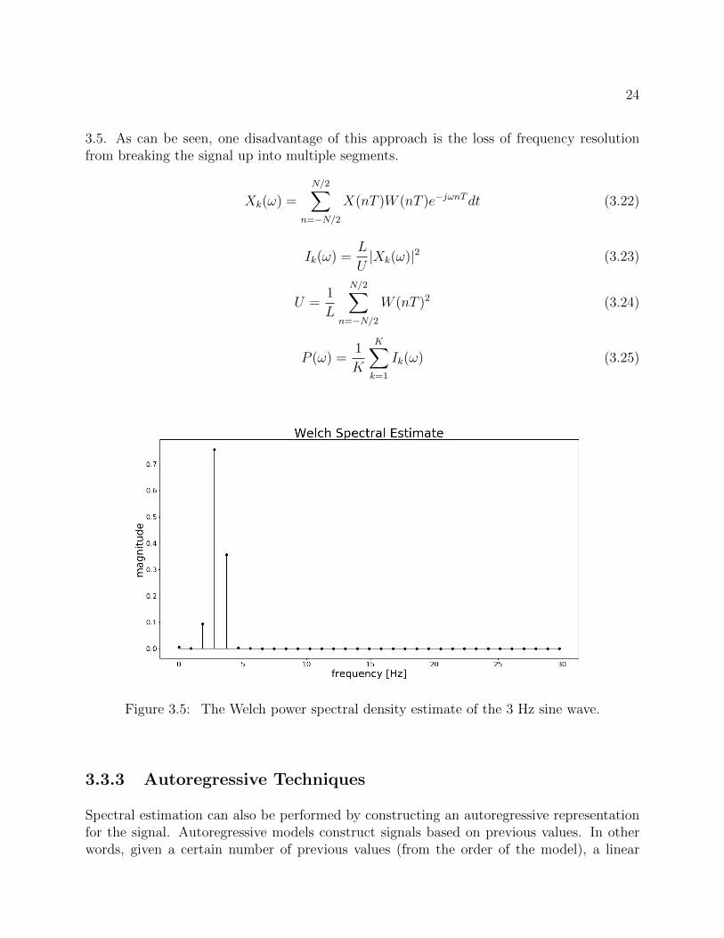
3.5 The Welch power spectral density estimate of the 3 Hz sine wave. . . . . . . 24
3.6 The autoregressive power spectral density estimate of the 3 Hz sine wave. . . 26
3.7 The db2 scale and wavelet functions. . . . . . . . . . . . . . . . . . . . . . . 28
3.8 The frequency response of the db2 scale and wavelet functions. . . . . . . . . 29
3.9 This figure shows two identical square waves sampled at different points. Thepoints marked with + indicate the first and last edge points selected for thesignal. . . . . . . . . . . . . . . . . . . . . . . . . . . . . . . . . . . . . . . . 30
3.10 This plot gives an example of models with high bias and high variance, as wellas a properly chosen model. . . . . . . . . . . . . . . . . . . . . . . . . . . . 32
3.11 This plot gives an example how regularization can prevent overfitting. . . . . 33
3.12 This shows an example of an MLP architecture neural network. . . . . . . . 36
viii

4.1 A schematic showing the wiring diagram and data collection for most of thedata. However, part of the testing set was measured from node 3 instead ofnode 1. . . . . . . . . . . . . . . . . . . . . . . . . . . . . . . . . . . . . . . . 39
4.2 A picture of the CAN bus is shown here. The Picoscope probes in this pictureare attached to node 3 in the top right. . . . . . . . . . . . . . . . . . . . . . 40
4.3 An example of the noise measured in one of the CAN bus nodes used for thisthesis. . . . . . . . . . . . . . . . . . . . . . . . . . . . . . . . . . . . . . . . 41
5.1 This plot shows an example of the calculated frequency spectrum from theChebyshev-windowed FFT. . . . . . . . . . . . . . . . . . . . . . . . . . . . . 47
5.2 This plot shows an example of the calculated frequency spectrum from theChebyshev-windowed FFT. . . . . . . . . . . . . . . . . . . . . . . . . . . . . 47
5.3 This plot shows an example of the calculated Welch estimate of the frequencyspectrum. . . . . . . . . . . . . . . . . . . . . . . . . . . . . . . . . . . . . . 48
5.4 This plot shows an example of the calculated frequency spectrum from au-toregressive model. . . . . . . . . . . . . . . . . . . . . . . . . . . . . . . . . 48
5.5 This plot shows the autoregressive fit for the noise sample for node 1. . . . . 49
5.6 This plot shows the autoregressive fit for the noise sample for node 2. . . . . 49
5.7 This plot shows the autoregressive fit for the noise sample for node 3. . . . . 50
5.8 This plot shows the calculated detail coefficients for the sample noise. . . . . 51
5.9 This plot shows the calculated approximation coefficients for the sample noise. 51
5.10 This plot shows the time-reversal asymmetry statistics for the first five lags. 52
5.11 A plot showing how the accuracy of the SVM changes as features are added(only including those features chosen as the final feature set for the SVM). . 54
5.12 A plot showing how the accuracy of the MLP changes as features are added(only including those features chosen as the final feature set for the MLP). . 55
6.1 This plot shows how the maximum allowable messages marked as rogue varieswith average time length based on constant false alarm probabilities of 1e−15and 1e− 11. . . . . . . . . . . . . . . . . . . . . . . . . . . . . . . . . . . . . 58
A.1 The overlayed histogram for all nodes. . . . . . . . . . . . . . . . . . . . . . 71
A.2 The overlayed histogram for all nodes. . . . . . . . . . . . . . . . . . . . . . 72
A.3 The overlayed histogram for all nodes. . . . . . . . . . . . . . . . . . . . . . 72
ix
A.4 The overlayed histogram for all nodes. . . . . . . . . . . . . . . . . . . . . . 72
A.5 The overlayed histogram for all nodes. . . . . . . . . . . . . . . . . . . . . . 73
A.6 The overlayed histogram for all nodes. . . . . . . . . . . . . . . . . . . . . . 73
A.7 The overlayed histogram for all nodes. . . . . . . . . . . . . . . . . . . . . . 73
A.8 The overlayed histogram for all nodes. . . . . . . . . . . . . . . . . . . . . . 74
A.9 The overlayed histogram for all nodes. . . . . . . . . . . . . . . . . . . . . . 74
A.10 The overlayed histogram for all nodes. . . . . . . . . . . . . . . . . . . . . . 74
A.11 The overlayed histogram for all nodes. . . . . . . . . . . . . . . . . . . . . . 75
A.12 The overlayed histogram for all nodes. . . . . . . . . . . . . . . . . . . . . . 75
A.13 The overlayed histogram for all nodes. . . . . . . . . . . . . . . . . . . . . . 75
A.14 The overlayed histogram for all nodes. . . . . . . . . . . . . . . . . . . . . . 76
A.15 The overlayed histogram for all nodes. . . . . . . . . . . . . . . . . . . . . . 76
A.16 The overlayed histogram for all nodes. . . . . . . . . . . . . . . . . . . . . . 76
A.17 The overlayed histogram for all nodes. . . . . . . . . . . . . . . . . . . . . . 77
A.18 The overlayed histogram for all nodes. . . . . . . . . . . . . . . . . . . . . . 77
A.19 The overlayed histogram for all nodes. . . . . . . . . . . . . . . . . . . . . . 78
A.20 The overlayed histogram for all nodes. . . . . . . . . . . . . . . . . . . . . . 78
A.21 The overlayed histogram for all nodes. . . . . . . . . . . . . . . . . . . . . . 79
A.22 The overlayed histogram for all nodes. . . . . . . . . . . . . . . . . . . . . . 79
A.23 The overlayed histogram for all nodes. . . . . . . . . . . . . . . . . . . . . . 79
A.24 The overlayed histogram for all nodes. . . . . . . . . . . . . . . . . . . . . . 80
A.25 The overlayed histogram for all nodes. . . . . . . . . . . . . . . . . . . . . . 80
A.26 The overlayed histogram for all nodes. . . . . . . . . . . . . . . . . . . . . . 80
x

List of Tables
2.1 A table outlining the published standards important for CAN communicationin cars. . . . . . . . . . . . . . . . . . . . . . . . . . . . . . . . . . . . . . . . 9
4.1 This table includes all the features extracted for analysis by the algorithm. . 43
4.2 A table containing the values used for the grid search to determine the bestvalues for the hyperparameters of the SVM. . . . . . . . . . . . . . . . . . . 45
4.3 A table containing the values used for the grid search to determine the bestvalues for the hyperparameters of the MLP. . . . . . . . . . . . . . . . . . . 45
5.1 This table shows features extracted from the example noise samples. . . . . . 52
5.2 This table includes all the features used by either algorithm. The ranking byeach filter algorithm is also shown (MC Ranking stands for multiple compar-ison ranking and OVR Ranking stands for one-versus-rest ranking). . . . . . 53
5.3 Confusion matrix for the best SVM configuration . . . . . . . . . . . . . . . 55
5.4 Confusion matrix for the best MLP configuration . . . . . . . . . . . . . . . 55
xi

Chapter 1
Introduction
1.1 Motivation
Security is always an important consideration for designing any system, and it is particularlyimportant when people’s lives are on the line, as is the case with automobiles. Car makersput a lot of effort into making their cars safe and frequently brag about crash safety ratingsin their advertisements. However, one area of safety that has lagged behind is in securing theController Area Network (CAN) bus, which is used for intra-vehicular communications. Carsare becoming more and more integrated with electronics, with some cars having more than50 electronic control units (ECUs) which control increasingly more powerful and complicatedsystems [1]. This increased complexity provides more vulnerabilities for exploitation, as wellas more potential control for hackers. Modern cars have control of safety-critical processesthrough the CAN bus, such as steering and braking. This creates safety concerns since itallows a malicious third party with access to the CAN bus to potentially take control of acar. This thesis proposes a way of identifying the signals of the different nodes, or ECUs,on a CAN bus in the interest of being able to help detect intrusions and malicious activityon the bus. In theory, similar processes should also be broadly applicable to other electroniccommunication systems.
CAN bus hacking has started to get a lot of attention in recent years. There is a lot ofpublicly available information regarding interfacing with and reverse engineering a car’sCAN bus. Additionally, many cheap, off-the-shelf products are available which assist in thisprocess. A simple internet search for “CAN bus hacking” returns over 17, 000, 000 results,with plenty of helpful and relevant information in at least the first two pages of results. Theseresults include a forum for discussing CAN bus protocol, projects requiring interfacing witha CAN bus from a variety of platforms, sharing code snippets, and more [2]; several articlesdiscussing how to interface with a CAN bus and highlighting off-the-shelf products [3, 4, 5,6, 7], including how to use an Arduino Uno equipped with a CAN shield [8] and a system
1

2
that can be bought for less than $20 which allows control of the CAN bus through the on-board diagnostics (OBD-II) port (including control of critical features such as steering andbraking) [9]; a blog detailing the design process for an “intelligent accessory control systemfor Jeep Wranglers” [10], including shared code, which directly uses the CAN bus to controlaccessories on the vehicle, such as the lights; a book titled The Car Hacker’s Handbook: AGuide for the Penetration Tester written by a security researcher [11]; and a company whichhosts car hacking challenges and conferences [12].
1.2 CAN Bus Hacking in the Literature
Since CAN packets are broadcast to all nodes on the bus and contain no built-in authen-tication, it is easy for components to both sniff the CAN network as well as pretend to bedifferent ECUs to send CAN packets. With cars becoming more and more sophisticated,they have begun to integrate things such as Bluetooth and cellular/Wi-Fi networks. Theseinterfaces provide access points for potential hackers to get into the CAN bus of a car [1].Consequently, car hacking is becoming a hot topic. Even the government has started to getinvolved [13].
Researchers from the University of Washington and the University California San Diegowere the first to begin the research into car hacking. They identified four main attack sur-faces for a car. These are the OBD-II port as a direct physical attack, the CD slot as anindirect physical attack, the Bluetooth stack as a short-range wireless attack, and the cellularmodem as a long-range wireless attack. The physical attacks, while disconcerting, are lessscary since access to hardware will always provide hacking or sabotage opportunities. Forinstance, they could always just cut some cables on the CAN bus if they wanted to disruptcommunication. However, they were able to remotely control some aspects of a vehicle bothby exploiting a vulnerability in the Bluetooth stack of an ECU and compromising a cellularmodem on the car, which fueled a lot of interest [14].
Inspired by this work, Miller and Valasek ([1], [15], [16], [17]) did extensive research intoCAN bus hacking and reverse engineered the CAN bus on multiple cars to demonstrate themost feasible attacks. They also released all their code and tools in order to assist futureresearchers. We will discuss some of the highlights from these papers; however, the readeris encouraged to explore them if more detail is desired.
Miller and Valasek began by investigating both a 2010 Ford Escape and a 2010 ToyotaPrius. They purchased the mechanic’s tools for these vehicles and went to work reverseengineering the CAN communication for each vehicle. Once they understood the meaning ofeach message and were able to figure out the appropriate checksum and security algorithms,they began injecting their own messages to see how the bus would respond. One area offocus for them was diagnostic messages since these are extremely powerful. To use diagnos-

3
tic messages, a diagnostic session must be begun with the intended ECU. To do so requiresan authentication via a cryptographic key. The ECU will send a seed, and the controllingECU must reply with the correct computed result. If this is successful, the ECU will entera diagnostic session. This allows extensive control over the ECU, including forcing it topretend it is receiving given sensor values or disabling certain features, such as the brakes.However, they found this to be difficult to use because while they were able to reverse en-gineer the cryptographic key, once the car started moving, diagnostic sessions could not beentered and any existing session would be terminated [1]. Despite this, they were still ableto demonstrate the ability to reprogram ECUs over the CAN bus; spoof dashboard readingssuch as speedometer, odometer, fuel remaining, and door ajar warnings; and even controlthe acceleration of the Toyota Prius [1]. Miller and Valasek then branched out to examiningseveral more cars, including mostly newer models (from 2014) and classified possible remoteattack surfaces (anything that performs wireless communication). These surfaces are listedand briefly explained below [15]:
• Passive Anti-Theft System - communication between chip in the ignition key anda device on the car; when the key is turned, its authenticity is verified through RFsignals
– Range: about 10 cm
– Usefulness for attack: very low - small range and worst case is to prevent car fromproperly starting
• Tire Pressure Monitoring System - transmits real-time tire pressure data to anECU
– Range: 1m
– Usefulness: low - small range, but it is possible to crash the associated ECU
• Remote Keyless Entry / Start - short-range, encrypted radio communication tounlock or start a vehicle
– Range: 5− 20m
– Usefulness: low - could potentially be used for theft purposes to unlock or startthe car without the proper key fob
• Bluetooth - intended for syncing a device, such as a phone, with the infotainmentsystem in a car
– Range: about 10m
– Usefulness: high - small range, but provides a reliable entry point to the automo-bile

4
• Radio Data System - intended for radio metadata for display (such as name of theradio station and song being played)
– Range: several miles
– Usefulness: moderate - difficult to successfully exploit
• Telematics / Cellular / Wi-Fi - connects the vehicle to a cellular radio for use withservices such as OnStar
– Range: Broad (as long as the car can have cellular communication)
– Usefulness: very high - large range; it may not have direct access to the CAN bus,but it can be used to transfer data
• Internet / Apps - provides connected features, such as apps and internet browsers
– Range: N/A
– Usefulness: very high - opens up the door for web browser exploits and maliciousapps
Miller and Valasek noted that safety-critical attacks generally require three stages. First, theattacker must gain access to an internal automotive network. Since the compromised nodewill likely not have direct control of the safety-critical features, the hacker will have to injectmessages through the CAN bus in order to control actions such as steering, accelerating,or braking. The final stage is to reverse engineer the CAN messages to understand how tocontrol the desired aspects of the vehicle [15]. Based on their analysis in this paper, theyselected the 2014 Jeep Cherokee for another attempt at reverse engineering messages andremotely controlling the vehicle. They demonstrated access to the cellular device on the Jeepfrom anywhere in the country, and were able to remotely control many important vehiclesystems, including steering, acceleration, brakes, and turning off the engine [16].
1.3 Intrusion Detection Systems
The National Institute of Standards and Technology (NIST) defines an intrusion as an at-tempt to compromise the confidentiality, integrity, and availability of a system by bypassingthe security mechanisms of a computer or network. To guard against this, intrusion detectionsystems (IDS) are generally constructed. Intrusion detection is the process of monitoringthe events occurring in a computer system or network and analyzing them for signs of in-trusions [18]. Classical intrusion detection methodologies can be classified in three majorcategories: Signature-based Detection (SD), Anomaly-based Detection (AD) and StatefulProtocol Analysis (SPA). Most IDS actually use a combination of multiple categories toprovide more robust and accurate detection [19]. Each of these categories will be explained,

5
and then a few proposed IDS for cars will be mentioned.
Signature-based detection, sometimes also called knowledge-based detection or misuse de-tection, looks for signatures, or patterns that correspond to a known attack or threat. SDrequires comparison of known patterns against a monitored traffic of events to look for thesesignatures [19].
Anomaly-based detection, also known as behavior-based detection, works based on the ‘nor-mal’ behavior of a system. In other words, it monitors activities on the network and looksfor irregularities. It would generally need to be given some parameters to monitor and thedistribution of those parameters under normal conditions. It then looks for deviations fromthat distribution in its observed network traffic. AD is often used alongside SD since SD willdetect known attacks, and AD will detect the unknown attacks [19].
Stateful protocol analysis, or specification-based detection, requires an IDS that understandsthe protocol. Similar to AD, it compares network traffic to normal profiles. However, whileAD looks at network-specific profiles, SPA uses vendor-developed generic profiles for specificprotocols based on the international standards for that protocol [19].
Based on their research, Miller and Valasek suggested some precautions to take when build-ing a CAN bus and what to look for to spot a potential attack. Their main suggestion forbuilding a CAN bus is, while total isolation between ECUs with remote functionality forthose which control safety-critical features may not be feasible, providing as much isolationas possible is a good idea. For example, the bus can be designed such that communica-tion between such ECUs must go through a bridge ECU, providing an additional layer ofsecurity. For intrusion detection, they suggest monitoring the rate of messages on a CANbus. Since most normal CAN packets will still be sent when a single node is compromised,the total messages will be a sum of the normal messages and the injected messages. Ad-ditionally, since the compromised node will generally not be the ECU typically controllingthe safety-critical features, the node that does control these features will still be sending itsnormal messages. In order to get the car to listen to the injected messages, injected messageswill need to be sent more frequently in order to make the car pay attention to them [15].This approach to intrusion detection was further investigated and suggested in [20, 15, 21,22]. Song et al added checking for recurring CAN ID in messages as a sign that a hackerwas injecting messages on the bus [22]. However, one issue with this is that, as Miller andValasek showed, once the initial node has been compromised, it is possible to incapacitatethe safety-critical ECU, which would greatly reduce the number of messages that would needto be injected [16]. Other methods that have been suggested include encryption [23] andinformation-theoretic measures such as entropy and relative entropy based on informationcontained in the message [24].
6
1.3.1 Approach
This thesis will take a rather different approach to intrusion detection. Miller and Valaseknoted that one of the main issues of analyzing CAN traffic is that there is no way to verify if amessage came from the expected ECU or an attacker via a different, compromised ECU [17].This thesis attempts to address that issue by “fingerprinting” the nodes on the bus so thatit can be known which node is sending each packet. By determining which node is sendinga message, any messages coming from an improper source can be identified as suspicious.For example, if a node from a telematics unit (such as OnStar), sends messages to controlbrakes or steering, this should instantly be marked as suspicious and untrustworthy.
We will perform this fingerprinting by analyzing the noise on the CAN bus. The idea be-hind this approach is that, although each node may have a theoretically identical transceiverwhich interacts with the bus, in reality, there will be slight differences between them due tothe existence of finite manufacturing tolerances. These differences will manifest themselvesat the smallest level, causing different patterns and likelihoods of “stray” electrons enteringthe bus as noise. Thus, when a particular node has control of the CAN bus, its unique noisepattern will be observable on the CAN bus. By monitoring the analog signal on the buslines, we will propose to recognize each node’s fingerprint. To do this, we treat the noise asa stochastic process and perform relevant statistical and signal analysis for characterizationand make use of machine learning algorithms to map these characterizations to a classifica-tion of which node is “speaking”.
This idea is similar to work done at Disney Research, where Yang and Sample are ableto recognize individual electronic devices of the same type and model by measuring andquantifying their unique electromagnetic “signatures” [25]. They do this by using a software-defined radio module to measure external electromagnetic interference (EMI) from electronicdevices. They then convert this to the frequency domain and store the most significant fre-quency magnitudes as the devices “EM-ID” [25]. They collect an EM-ID from each of thedevices and store this in a database. To identify a device, they measure its external EMI andcompare this to their database of EM-IDs. In their tests, they were able to identify deviceswith accuracies varying between 72% to 100%, depending on the device type [25].
This approach is not necessarily meant to be a replacement for traditional intrusion de-tection approaches. While it has potential to be a key component of intrusion detectionsystems, it is easy to envision it being combined with traditional approaches, such as asearch for known attack signatures, in order to create an even more robust system.
In order to perform this classification, it is necessary to understand the process which gen-erates noise, appropriate models for noise, how these models can be leveraged to extractfeatures (ie, representative information describing the signal), and methods of learning dif-ferences between the features describing each node. The theory behind the methods used

7
for all of these things and the reason for choosing each method will be explained later.
The rest of this thesis is outlined as follows. Chapter 2 will discuss the CAN bus proto-col. A brief history will be given (2.1), relevant standards will be mentioned (2.2), someadvantages of the CAN protocol, such as its strong noise immunity, will be discussed (2.3),and the packet structure will be outlined and discussed (2.4). Chapter 3 will discuss the bulkof the relevant theory used for characterization and classification of the signals in this thesis.This will involve discussions on statistical analysis techniques, including hypothesis testing(3.1); stochastic models and types of noise (3.2); frequency analysis (3.3), wavelet analysis(3.4); additional features of interest (3.5), learning algorithms for classification (5.3); andfeature selection techniques (5.2). Chapter 4 will discuss a proposition for how to fingerprintnodes on a CAN bus. All steps used in classifying the nodes - including preprocessing, fea-ture extractions, training, and testing - will be discussed there. Chapter 5 will present theresults obtained using the test CAN bus. An example of the measured noise and each of theresulting features will be presented. This thesis will close with a discussion on some issuesregarding a physical implementation and a review of what’s been accomplished in Chapter6.

Chapter 2
CAN Bus Technology
2.1 Beginnings
Development of the CAN bus began in 1983 by engineers at by Robert Bosch GmbH to meetthe needs of automotive engineers. The CAN bus was first introduced in 1986, providinga multi-master system with non-destructive arbitration to provide priority for the mostimportant messages, as well as error handling and the automatic disconnection of faultynodes. By mid 1987, Intel had already created the first CAN controller chip [26]. In 1991,the Mercedes W140 was the first car to include a CAN network, connecting five ECUs [27].In 1993, version 2.0 of the Bosch CAN specification was standardized in ISO 11519-2, addinga desccription of the physical layer of the CAN bus, and an addendum was added with ISO11898 in 1995, adding an extended frame format with a CAN identifier extension [26].
2.2 Standards
CAN bus has many associated standards that have been published by the InternationalStandards Organization (ISO) and the Society of Automotive Engineers (SAE). The mostrelevant of these standards for cars are listed and briefly explained in Table 2.1.
2.3 Advantages
The Controller Area Network (CAN) bus is a robust communication protocol designed tobe resistant to electrical interference. The protocol implements twisted pair, balanced line,differential signaling, and (sometimes) electrical shielding to provide good noise immunity.It also uses a synchronization protocol to ensure nodes on the bus are all in agreement about
8

9
ISO 11898 series The main CAN standard specifying the physical and datalink layers of CAN for use in road vehicles [28, 29, 30]
ISO 16845 series Provides methodology for testing an implementation’sconformance to ISO 11898 [31, 32]
ISO 15765 series Specifies diagnostics for CAN vehicle network systemsspecified in ISO 11898 [33, 34, 35]
J2284 series SAE Recommended Practice defining the Physical Layerand portions of the Data Link Layer for High-SpeedCAN, including for use with CAN Flexible Data-rate(CAN FD) up to 5 Mbit/s1 [36, 37, 38, 39, 40, 41]
J2411 SAE Recommended practice defining the Physical Layerand portions of the Data Link Layer for a single-wireCAN network [42]
Table 2.1: A table outlining the published standards important for CAN communication incars.
the data being sent on the bus. This allows for communication speeds from 50 kbit/s up to1Mbit/s at bus lengths from 40m (at 1Mbit/s) to 1 km (at 50 kbit/s). For these reasons,it is the main choice for communication between different electronic control units (ECU) oncars and is also often chosen for use in other fields, such as robotics.
The combination of balanced line, twisted pair, and differential signaling is crucial to thehigh noise immunity provided by CAN bus. That the lines are balanced means there is equalbut opposite current flowing in each signal line. This gives a field-canceling effect preventscross-talk between the wires. Additionally, since external noise sources generally result fromcoupling of electrical and magnetic fields, the use of twisted pair causes external noise sourcesthat are sufficiently far away to affect each line equally. This is because the twisting causesthe noise source to see an approximately equal amount of each wire. Combining this withdifferential signaling through twisted pair CANH and CANL (CAN high and CAN low) linesprovides strong external noise immunity through the use of strong common mode rejection.Any common noise from external sources is subtracted out, giving a stable differential signaland allowing for reliable communication.
Furthermore, signal reflections are prevented through the use of 120 Ω terminating resistors,which are specified to match the characteristic impedance of the line [43]. This is necessarysince mismatched impedances can cause reflections back from the higher impedance towardsthe lower impedance. Current, like most things in nature, prefers to take the path of leastresistance. The characteristic impedance of a transmission line can be calculated by equation2.1, where L is inductance per unit length and C is capacitance per unit length [44].
Z =
√L
C(2.1)

10
The CAN bus also implements a synchronization protocol that keeps the bit rates of thereceiving nodes aligned with the rate of the transmitting node. Nodes are synchronized onthe bit edges to keep a frequent update and prevent nodes from drifting apart. To help this,bit stuffing is implemented. This means that, whenever there are 5 consecutive same bits,a bit of the opposite kind is stuffed in to keep the nodes in sync. This bit is ignored whenparsing the message [45].
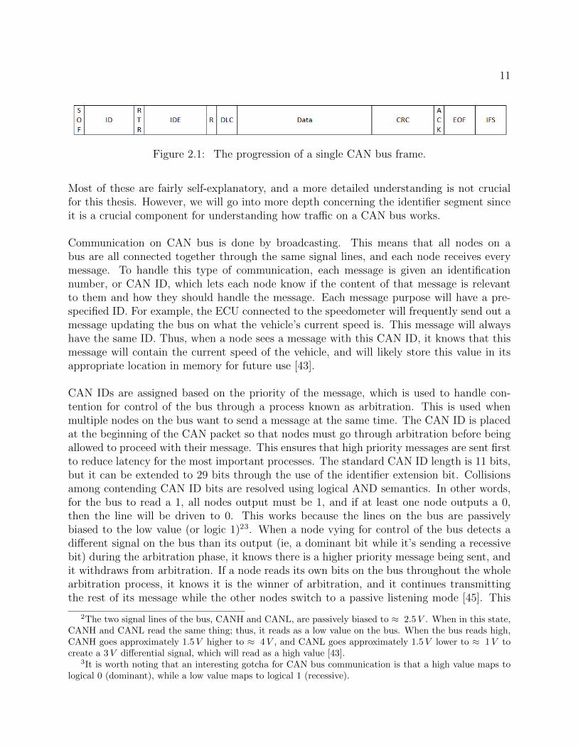
2.4 Packet Protocol
A packet on the CAN bus consists of different frames, which are shown in Figure 2.1 andoutlined below [43]:
• Start of Frame (SOF) - single dominant bit indicating the beginning of a packet
• Identifier (ID) - establishes priority (the lower the binary value, the higher the pri-ority) and purpose for the message
• Remote Transmission Request (RTR) - dominant when information is requiredfrom another node via a response
• Identifier Extension (IDE) - dominant indicates no extension; recessive indicatesmore identifier bits will follow
• Reserved Bit (R) - for possible use by future amendment
• Data Length Code (DLC) - 4 bits, contains number of bytes of data being trans-mitted
• Data - up to 64 bits of data
• Cyclic Redundancy Check (CRC) - checksum for error detection
• Acknowledgement (ACK) - every node receiving an accurate message submits adominant bit; if a node detects an error and leaves this bit recessive, the message isignored and a retransmission is attempted
• End of Frame (EOF) - 7 (recessive) bits marking the end of the frame (not stuffed)
• Interframe Space (IFS) - minimum of 7 (recessive) bits between frames (not stuffed)
11
Figure 2.1: The progression of a single CAN bus frame.
Most of these are fairly self-explanatory, and a more detailed understanding is not crucialfor this thesis. However, we will go into more depth concerning the identifier segment sinceit is a crucial component for understanding how traffic on a CAN bus works.
Communication on CAN bus is done by broadcasting. This means that all nodes on abus are all connected together through the same signal lines, and each node receives everymessage. To handle this type of communication, each message is given an identificationnumber, or CAN ID, which lets each node know if the content of that message is relevantto them and how they should handle the message. Each message purpose will have a pre-specified ID. For example, the ECU connected to the speedometer will frequently send out amessage updating the bus on what the vehicle’s current speed is. This message will alwayshave the same ID. Thus, when a node sees a message with this CAN ID, it knows that thismessage will contain the current speed of the vehicle, and will likely store this value in itsappropriate location in memory for future use [43].
CAN IDs are assigned based on the priority of the message, which is used to handle con-tention for control of the bus through a process known as arbitration. This is used whenmultiple nodes on the bus want to send a message at the same time. The CAN ID is placedat the beginning of the CAN packet so that nodes must go through arbitration before beingallowed to proceed with their message. This ensures that high priority messages are sent firstto reduce latency for the most important processes. The standard CAN ID length is 11 bits,but it can be extended to 29 bits through the use of the identifier extension bit. Collisionsamong contending CAN ID bits are resolved using logical AND semantics. In other words,for the bus to read a 1, all nodes output must be 1, and if at least one node outputs a 0,then the line will be driven to 0. This works because the lines on the bus are passivelybiased to the low value (or logic 1)23. When a node vying for control of the bus detects adifferent signal on the bus than its output (ie, a dominant bit while it’s sending a recessivebit) during the arbitration phase, it knows there is a higher priority message being sent, andit withdraws from arbitration. If a node reads its own bits on the bus throughout the wholearbitration process, it knows it is the winner of arbitration, and it continues transmittingthe rest of its message while the other nodes switch to a passive listening mode [45]. This
2The two signal lines of the bus, CANH and CANL, are passively biased to ≈ 2.5V . When in this state,CANH and CANL read the same thing; thus, it reads as a low value on the bus. When the bus reads high,CANH goes approximately 1.5V higher to ≈ 4V , and CANL goes approximately 1.5V lower to ≈ 1V tocreate a 3V differential signal, which will read as a high value [43].
3It is worth noting that an interesting gotcha for CAN bus communication is that a high value maps tological 0 (dominant), while a low value maps to logical 1 (recessive).

12
Figure 2.2: An example of arbitration on the CAN bus. In this scenario, node 3 wins thearbitration and continues with the rest of the message.
arbitration process is shown in Figure 2.2.
There are four message types on the CAN bus. They are: data frames (for transmittingdata), remote frames (for requesting data), error frames (for flagging a detected error), andoverload frames (for requesting an extra delay when a node is too busy) [43]. In order tounderstand how information is communicated on the CAN bus, we can ignore the less com-mon error and overload frames and focus on data and remote frames. These message typesare used by cars in three important ways. The standard data frame is used in an informa-tive capacity. For example, the Power Steering Control Module (PSCM) will periodicallybroadcast the current position of the steering wheel. This kind of message does not haveany physical effect - it simply is used to update values in memory. Another use is to requestsome sort of action from another ECU. For example, if the Adaptive Cruise Control (ACC)module determines the brakes need to be applied, it would request this action over the CANbus. The third usage is even more powerful - diagnostic messages. Diagnostic messages areintended for communication between a mechanic’s tool and ECUs. They can request thatan ECU perform a test action or get diagnostic information. However, since they are onlymeant for use in a repair shop, these messages are usually ignored by a car in motion toprevent dangerous actions [17].
An example of a data frame CAN message with an ID of 0x602, collected with a Pico-scope 5000 series oscilloscope, is displayed in Figure 2.3. A zoomed-in view of the identifier

13
section is displayed, and dotted lines indicate each bit. The bit marked by the gray hexagonabove the hexadecimal values is a stuffed bit. In this case, the 0x6 in the identifier signals adata transfer, while the 0x02 indicates it is for the node associated with the identifier 0x024.
(a) An example data frame on a CAN bus. The message content is displayed in hexadecimal abovethe waveform.
(b) The identifier section of the CAN packet.
Figure 2.3: An example of a collected data packet from the CAN bus. A zoomed-in view ofthe identifier is shown.
4It is worth noting that cars are not necessarily likely to allocate their identifier in the same manner.
Chapter 3
Theory
3.1 Statistical Analysis
Any signal processing application always requires a thorough treatment of statistics. In thisthesis, we are attempting to classify signals from different nodes on a CAN bus. This willrequire identification of some traits, or features, of the measured signal that consistentlyproduce different values for each of the nodes. A feature can be evaluated for its discrimi-natory power based on statistical differences between the populations of a feature for eachnode. This section will discuss background regarding the concept of statistical populationsand hypothesis testing for differences between populations.
3.1.1 Populations and Random Variables
In order to explain the relevant statistical analysis techniques, we will start by giving a back-ground on statistical populations. This will provide necessary background for understandinghow stochastic processes, such as noise, can be modeled, as well as how to differentiate be-tween two (or more) different stochastic processes. In statistics, a population refers to theset of all items or events that represent something of interest to an experiment. For example,when drawing cards from a deck, the population would be the set of all cards in the deck.For convenience, a random variable is used to map items or events from a population to thereal number line [46]. Continuing with the deck of cards example, we have a few choices forour random variable depending on what is of interest to the experiment. For example, wecould decide that all we care about is the value of the card and not its suit or color. In thiscase, we could give all 2’s a value of 2, all 3’s a value of 3, etc. Alternatively, if we care aboutthe suit, we could number each card 1-52, and the random variable would take on the valueof whatever number had been assigned to a specific card. Depending on how we define therandom variable, it will have some governing probability distribution which maps values of
14

15
the random variable to a probability of occurring. For the deck of cards, we would likely bedealing with a uniform distribution since each card is equally likely to be drawn.
Probability distributions can be described using probability mass or density functions. Prob-ability mass functions (pmf) are used to describe discrete random variables, such as the cardsfrom the last paragraph, where each value of f(x) maps to a probability of observing thevalue x. Probability density functions (pdf) describe continuous random variables, such asa distance between two objects. For a continuous random variable, the probability of anyspecific value occurring is 0, so f(x) gives a probability density for values around x. To geta probability, one must look at a range of values for x and find the integral for f(x) overthat range. Sometimes it is also convenient to deal with cumulative distribution functions(cdf). This function gives the probability of observing a value less than or equal to x. Inother words, for the continuous case, we would define the cdf F (x) as in equation 3.1 [46].
F (x) =
∫ x
−∞f(x)dx (3.1)
Important properties of random variables and distributions include expected value, vari-ance, covariance, correlation. The expected value of a random variable is defined as theweighted average of the random variable given, by equation 3.2. For an infinite sample, thiswould be equivalent to the mean. The variance of a random variable describes the averagesquared distance from the mean and is given in equation 3.3. Variance is the square of themore frequently used standard deviation. If we want to compare random variables, we canuse covariance or correlation, which is a linear measure of the relationship between two ran-dom variables. Correlation is basically a scaled covariance, guaranteed to be between [−1, 1],used to gain an intuitive understanding of how closely two variables are related. These areshown in equations 3.4 and 3.5. When dealing with time series, we often talk about auto- andcross-covariance, shown in equations 3.6 and 3.7, which define the relationship at differenttime lags [47].
E[X] =
∫ ∞−∞
xf(x)dx (3.2)
V[X] = E[(X − E[X])2] (3.3)
C[X, Y ] = E[(X − E[X])(Y − E[Y ])] (3.4)
ρ =C[X,Y]√V[X]V[Y ]
(3.5)
CXX(τ) = E[(Xt1 − E[Xt1 ])(Xt1+τ − E[Xt1+τ ])] (3.6)
CXY (τ) = E[(Xt1 − E[Xt1 ])(Yt1+τ − E[Yt1+τ ])] (3.7)

16
A distribution of general interest, which is also quite relevant to this thesis, is the nor-mal (Gaussian) distribution, with probability density function given in 3.8. The Gaussiandistribution is so relevant thanks in large part to the central limit theorem, which states thatthe limiting distribution for any random variable defined as the summation of many inde-pendent random variables, no matter what their underlying distribution, will be a Gaussiandistribution [46].
P [X = x] =1√
2πσ2e−(x−µ)2
2σ2 (3.8)
3.1.2 Hypothesis Tests
Now that we’ve built a little bit of background, we can start talking about applying sta-tistical principles to hypothesis tests. Hypothesis tests are important for understandingsimilarities and differences between statistical populations. Hypothesis tests will be usedlater to evaluate features. Features which provide statistically significant differences be-tween the populations of each node are identified as features with discriminatory power andare thus desirable for use in the classification of the nodes.
Hypothesis tests are a set of statistical tests which give a probability, or p-value, of someobservation given a set of conditions or assumptions. In general, p-values test a “null hy-pothesis” (H0). The p-value gives a probability of observing the data (or more extreme) ifH0 is assumed to be true. It makes sense, then, that a low p-value indicates we should berather suspicious of the null hypothesis, while a high p-value indicates that H0 is at leastplausible. A commonly accepted significance level is α = 0.05, which means that we willreject the truth of the null hypothesis at p < α. In this section we will discuss some relevanthypothesis tests. We’ll begin with the independent samples t-test, then move on to theKolmogorov-Smirnov (KS) test.
The independent samples t-test is used for testing the difference between the mean of twopopulations (assuming they are approximately normally distributed). It is perhaps the mostcommonly used test for evaluating the difference between two populations. The null hy-pothesis is generally µ1 = µ2 (the means of the two populations are equal). It uses the teststatistic shown in equation 3.9, where Xk is sample k, s2
pooled is the pooled variance estimate,and Nk is the number of data points in sample k. Pooled variance is found by equation3.10, where s2
k is the variance of sample k and dfk = Nk − 1 is the number of degrees offreedom. Assuming the two means are equal, this test statistic follows what is known as a tdistribution with dftotal = df1 + df2 degrees of freedom. Thus, the value of t can be turnedinto a p-value based on where it falls within its t distribution. This p-value represents theprobability of observing the found difference between the two means or more extreme (larger
17
difference), assuming that the means are actually equal.
t =X1 − X2√
s2pooledN1
+s2pooledN2
(3.9)
s2pooled =
df1s21 + df2s
22
dftotal(3.10)
The KS test is a test for differences between two statistical distributions. It makes noassumption on the distribution for either population, which makes it useful for populationswith unknown distribution. It works using the test statistic shown in equation 3.11, which isthe maximum distance between two cdfs weighted by the square root of the number of sam-ples n. This statistic follows a Kolmogorov distribution, which has the cdf shown in equation3.12 [48]. This value is turned into a p-value by evaluating the Kolmogorov distribution.Details for this can be found in [49].
D =√n supx∈R|F2(x)− F1(x)| (3.11)
P [D ≤ t]→ H(t) = 1− 2∞∑i=0
(−1)i−1e−2i2t (3.12)
3.2 Noise Models
This section will extend the statistical discussion to discuss stochastic processes. We willdiscuss some models for how values in a population are generated, with an eye towardsspecifically how noise may be modeled as a stochastic process. We will then mention someexisting mathematical models related to noise in semiconductor devices.
3.2.1 Stochastic Models
There are many different stochastic process theories which have been developed that applywell to random noise. Understanding these processes and their models will give good insightfor how to approach feature extraction. Some highlights of stochastic processes that havebeen used to describe noise include the Markov process, martingale, Poisson process, andGaussian process. We will start by discussing the Markov property and Martingales, thenmove on to Poisson and Gaussian processes. As it will be seen, these processes are all quiterelated.
A Markov process is any process that has the Markovian property, which is shown in equation
18
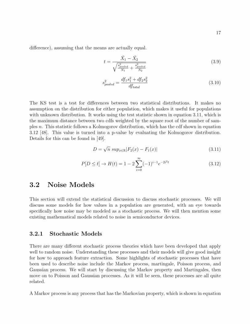
3.13. In words, it essentially says that future states depend only on the current state. Thisis taken a step further with martingales, which place restrictions on the expected value offuture values. The martingale, submartingale, and supermartingale are defined in equation3.14, where, in all cases, the expected value is assumed to be finite [50]. A good example ofa process that can have all of these properties is the random walk, which has a huge numberof applications from noise [51, 52] to neural activity [53]. This process is often explained bycomparing it to a drunk person trying to walk. Simplifying to one dimension, we can thinkof a drunk person trying to walk forward. In his or her drunkenness, he or she may take astep either forward or backward. In the case that each of these is equally likely, it is calleda zero-mean random walk (which is also a martingale). A graph of this is shown in Figure3.1.
P [xn = j|Xn−1 = i,Xn−2 = k, ..., X0 = l] = P [Xn = j|Xn−1 = i] (3.13)
E[xn|Xn−1 = i,Xn−2 = k, ..., X0 = l] = Xn−1 ∀ n ≥ 2 (3.14a)
E[xn|Xn−1 = i,Xn−2 = k, ..., X0 = l] ≤ Xn−1 ∀ n ≥ 2 (3.14b)
E[xn|Xn−1 = i,Xn−2 = k, ..., X0 = l] ≥ Xn−1 ∀ n ≥ 2 (3.14c)
Figure 3.1: An example of a zero-mean random walk.
A Poisson process is any process which follows 5 basic assumptions. For each t ≥ 0, whereNt is an integer-valued random variable which can be thought of as representing a numberof arrivals, we have:

19
1. N0 = 0 (start with no arrivals)
2. s < t ⇒ Ns and Nt − Ns are independent (arrivals in disjoint time periods are inde-pendent)
3. Ns and Nt−s are identically distributed (number of arrivals depends only on periodlength)
4. limt→0P [Nt=1]
t= λ (arrival probability is proportional to period length if the length is
small)
5. limt→0P [Nt>1]
t= 0 (no simultaneous arrivals)
Any such process will have an Nt that follows the Poisson distribution (for any given t) withpmf shown in equation 3.15 [46]. As can be seen from property 3, any Poisson process isan example of a supermartingale since future arrivals don’t depend on past arrivals and Nt
can obviously only get larger as t increases. The parameter lambda is generally given by arate of arrival multiplied by the length of time, and Nt will represent the distribution for thenumber of arrivals in that time frame. Noise can be modeled to be the result of a Poissonprocess since it is the result of discrete electron “arrivals” [52, 51, 53, 54, 55].
P [Nt = n] = e−λt(λt)n
n!(3.15)
The Gaussian process is perhaps the most common process observed in nature, thanks tothe central limit theorem, as described earlier. Since observed noise is generally the result ofmany atomic-level events coming together, it is well-modeled by a Gaussian [47]. This alsofollows from noise’s interpretation as a Poisson process since a Poisson distribution is wellapproximated by a Gaussian for large λ (ie, when the rate of arrival is large and Nt modelsa sum of large numbers of independent arrivals over a given time period). The Gaussiandistribution is presented in equation 3.8 [46]. The Gaussian property of noise is used bymany important applications, such as the Kalman filter’s Gaussian assumption [56].
3.2.2 Physical Origins
Electrical noise occurs in part due to the discrete and probabilistic nature of charge andmatter at small scales. Observed noise is the result of averages over the randomness of alarge number of particles. Interference from electric fields both within electrical devices andfrom outside sources also plays a role in contributing to noise. There are three main types ofelectrical noise - thermal noise, shot noise, and flicker noise. In general, all three types can bemodeled as Gaussian processes. This section will give only a brief overview of each of these

20
three types of noise. For more detailed explanations, the reader is encouraged to explore [47].
Thermal noise is the result of random thermal motion, and can be understood by treat-ing the particles as an ideal gas. Any two-terminal linear electrical circuit with a purelyresistive impedance will display thermal noise which depends only on resistance and tem-perature. For measurable frequencies and normal temperature ranges, the spectral contentof current fluctuations due to thermal noise can be accurately represented by equation 3.16,where T is temperature, k is Boltzmann’s constant, and R is its resistance. Since Boltz-mann’s constant is so small, (1.38 ∗ 10−23), this will likely be only a very small amount ofany measured noise [47].
Sth(f) =2kT
R(3.16)
Shot noise can be present in any device which contains some potential barrier. Noise iscreated whenever an electron gains sufficient energy to cross this barrier. The stochasticmodel for shot noise current is given by equation 3.17, where q is the charge of an electron,N(t) is the number of electrons which have crossed a potential barrier at time t (with crossingtimes ti) as modeled by a Poisson process, and δ is the Dirac-delta function. The spectraldensity of the current may be time-varying and is given by equation 3.18, where VT = kT/q.[47].
Q(t) = qN(T ) (3.17a)
I(t) =dQ(t)
dt=∑i
qδ(t− ti) (3.17b)
Ss(t, f) = qIs(eV/VT + 1) (3.18)
Flicker noise refers to excess noise observed at low frequencies that can’t be explained bythermal or shot noise. It is observed in many different phenomena aside from just electricalnoise. Since it is often inversely proportional to frequency, flicker noise is sometimes referredto as 1/f noise. The characteristics of flicker noise often differ from device to device, evenfor two of the same type of devices from the same die. Various theories have been proposedfor flicker noise in many different electronic components, each resulting in slightly differentmodels. From experimental work, the time-invariant spectral density of flicker noise is oftenmodeled as shown in equation 3.19, where K is a device-specific constant, a is a constant in[0.5, 2], and b is a constant approximately equal to 1 [47].
S1/f (f) = KIa
f b(3.19)

21
3.3 Frequency Analysis
As shown above in section 3.2.2, each of the types of electrical noise has an associatedfrequency domain representation which depends on some device-specific parameters. Sincemeasuring these parameters to the necessary resolution would be extremely difficult if notimpossible and, in the case of flicker noise, the exact physical origins of these parameters areunknown, it makes sense to look for differences in the frequency estimates of the measurednoise to assist with identifying device-related differences between the generated noises. Thissection will first discuss the Fourier transform. Building upon the Fourier transform aremany different spectral estimation techniques that are designed to give better estimates ofthe spectral content of a signal based on certain assumptions. Here, we will discuss two ofthese - Welch’s estimation using averaging and a technique which uses autoregressive modelfitting.
3.3.1 Fourier Transform
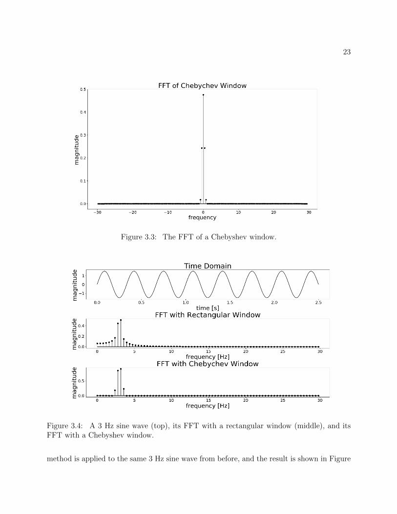
The Fourier transform, shown in equation 3.20, is one of the most basic techniques forfrequency analysis. It uses the complex exponential to split up a signal into a summationof sines and cosines of different frequencies. In practice, we use a finitized and discretizedversion of this transform shown in equation 3.21) [57] (more specifically, we use the FastFourier Transform algorithm [58] for computations). The effects of discretizing and finitizingthis transform are well-studied. Taking a finite time segment for a signal is the same asmultiplying the infinite signal by a rectangular window function defined on t ∈ [−T/2, T/2].It can be shown that multiplication in the time domain is equivalent to convolution in thefrequency domain, so the result of an FFT will give the true frequency representation of oursignal convolved with the frequency representation of the window. This creates leakage inthe result of the FFT, which essentially means that any frequencies present in the signalbecome spread out through neighboring frequencies in the FFT according to the FFT of thewindow. For the rectangular window, this results in leakage in the form of the sinc functionas shown by its FFT in Figure 3.2. To help mitigate these effects, one can choose a differentwindow for the data, such as Chebyshev, Hamming, or Hann. For example, a pure sine waveof frequency 2 Hz contains only one frequency. However, cutting it off in a finite rectangularwindow (that is not a multiple of its period in length), gives significant leakage in the FFT.This effect is shown in Figure 3.4, where, for the purposes of this example, we contrast theuse of no window (a rectangular window) with that of a Chebyshev window (whose FFTis shown in Figure 3.3) to show how this can significantly improve our frequency estimate.The Chebyshev window is chosen for use in this thesis based on its combination of low sidelobe level while maintaining a relatively thin main lobe. Since frequency magnitudes will belooked at individually, it is especially important to eliminate the bias in estimates due tospectral leakage. Thus, the Chebyshev window was parameterized to give 90 db of side lobe

22
attenuation (α = 4.5). Further investigation of windows can be found in [57].
X(ω) =
∫ ∞−∞
X(t)e−jωtdt (3.20)
X(ω) =
N/2∑n=−N/2
X(nT )e−jωnT (3.21)
Figure 3.2: The FFT of a rectangular window.
3.3.2 Welch’s Method
Another common method for estimating spectral density is Welch’s method. This methodis an attempt to compensate for randomness when only one signal is present. This canoften give improved estimates over a simple FFT and is a logical starting point for spectralestimation without requiring known signal parameters. Welch’s method works by assumingstationarity of the signal and breaking the data up into K possibly overlapping segments oflength L. These segments are windowed, and the Fourier of each segment is taken as normal.The spectral estimate is obtained by taking the average value of the squared magnitude foreach frequency. This process is shown in equations 3.22-3.25, where X is the signal, Xk isthe kth segment, W is the window, I is the periodogram (squared-magnitude of the FFT)for each segment, and P is the spectral estimate of the signal [59]. For comparison, Welch’s
23
Figure 3.3: The FFT of a Chebyshev window.
Figure 3.4: A 3 Hz sine wave (top), its FFT with a rectangular window (middle), and itsFFT with a Chebyshev window.
method is applied to the same 3 Hz sine wave from before, and the result is shown in Figure
24
3.5. As can be seen, one disadvantage of this approach is the loss of frequency resolutionfrom breaking the signal up into multiple segments.
Xk(ω) =
N/2∑n=−N/2
X(nT )W (nT )e−jωnTdt (3.22)
Ik(ω) =L
U|Xk(ω)|2 (3.23)
U =1
L
N/2∑n=−N/2
W (nT )2 (3.24)
P (ω) =1
K
K∑k=1
Ik(ω) (3.25)
Figure 3.5: The Welch power spectral density estimate of the 3 Hz sine wave.
3.3.3 Autoregressive Techniques
Spectral estimation can also be performed by constructing an autoregressive representationfor the signal. Autoregressive models construct signals based on previous values. In otherwords, given a certain number of previous values (from the order of the model), a linear

25
prediction, or regression, is used to generate the next value. For such signals, autoregressivetechniques can give good spectral estimates. A downside of this technique is it requires apriori knowledge of a parameter for the signal - the autoregressive order. However, there areways for estimating this, such as in [60]. An IIR filter driven by a serially independent noisesequence would produce an autoregressive signal. Then, since analog filters, often includedon CAN bus lines and transceivers, as well as any data acquisition system, are generally IIRfilters, this model makes sense for use in estimating the spectral content of the measurednoise on the CAN bus.
The autoregressive spectral technique is constructed under the assumption of a non-deterministic,weakly stationary time series X(n). Under this assumption, X(n) can be represented by the(M + 1)th order autoregressive model in equation 3.26, where ε is white noise. The char-acteristic equation of this form is given in equation 3.27. To compute the power spectraldensity, we estimate the coefficients using the covariance method, which uses a least-squaresmethod to solve equation 3.28. The variance - found with equation 3.29, where CXX is theauto-covariance function - is also used to scale the spectral estimate. The power spectraldensity estimate is then given by equation 3.301 [61]. For reference, the 3rd order autore-gressive PSD estimate of the 3 Hz sine wave is shown in Figure 3.6. With this method, wedon’t lose any frequency resolution. It is worth noting that this signal does not meet ourassumptions for the construction of this estimate; thus, any comparison with the previousmethods should be taken with a grain of salt.
X(n) = ε(n) +M∑m=1
amX(n−m) (3.26)
0 = 1−M∑m=1
amzm (3.27)
CXX(l) =M∑m=1
amCXX(l −m) (3.28)
S2(M) = CXX(0)−M∑m=1
amCXX(m) (3.29)
ˆpxx(f) =S2(M)
|1−∑M
m=1 ame−i2πfm|2
(3.30)
1This is an estimate of the autospectrum of X(n), pxx =∑∞l=−∞ CXX(l)e−i2πfl.

26
Figure 3.6: The autoregressive power spectral density estimate of the 3 Hz sine wave.
3.4 Wavelet Analysis
Wavelets originated as an extension of the Fourier Transform to finite, orthonormal ba-sis functions. The original wavelet, Morlet’s wavelet, was a continuous wavelet transformwhich was made to be an alternative to the short-time Fourier transform (STFT) for time-frequency analysis. Morlet wanted precise time resolution for high-frequency signals, as wellas precise frequency resolution for low-frequency signals. Due to inputs from researchers invarious fields from quantum mechanics to electrical engineering, wavelets have since grownand evolved to encompass many more applications. For example, the discrete wavelet trans-form (used in this thesis)2 is often used to perform subband FIR filtering [62].
Wavelets have been shown to be a good feature to extract for time series classification [63].Due to their finite nature, wavelets are able to provide local signal information that would bemissed by the previously discussed frequency analysis techniques. Additionally, this makeswavelets much more useful for approximating choppy data with sharp discontinuities (eg,noise) than a Fourier transform [64]. For these reasons, wavelets are chosen to complementthe frequency analysis to provide more complete statistical representations of the data.
The discrete wavelet transform was created by Ingrid Daubechies in 1988. It is made up
2It is worth noting that the discrete wavelet transform is not the same as a discretized continuous wavelettransform. Continuous wavelet transforms may be calculated discretely. There is actually a significantdifference between the analysis for continuous wavelet transforms and discrete wavelet transforms.

27
of two functions - a scale function and a wavelet function, sometimes called the father andmother wavelets, respectively. Each is convolved with the data to generate N
2coefficients
(where N is the number of data points) since the convolution is done by sliding with a factorof two (in other words, every other value is skipped). The scale function gives what is knownas approximation coefficients, which can be thought of as a lower dimensional approximationof the original data, while the wavelet function gives detail coefficients, which contain therest of the information from the original signal that is not contained in the approximationcoefficients. If desired, this process can then be repeated on each new set of approximationcoefficients until there are not enough coefficients remaining to perform another transform.This repetition is known as a multiresolution analysis, with each successive transform givinganother layer of decomposition [65].
A wavelet must be chosen for the analysis. Since noise is generally sharp rather than smooth,smoother wavelets with more vanishing moments3 are discarded, eliminating symlets. Ad-ditionally, since both the approximation and detail coefficients will be used, it is believedthat it is unnecessary to have vanishing moments from both the mother and father wavelets,eliminating coiflets. Of the most commonly used discrete wavelets, this leaves Daubechies4 tap wavelet (db2 for its 2 vanishing moments) from Ingrid Daubechies’ original discretewavelets as an appealing choice.
Daubechies 4 tap wavelet transform is given by the orthonormal basis in its scaling andwavelet coefficients in equations 3.31 and 3.32. The associated multiresolution analysis isgiven by equations 3.33 and 3.34, where the first subscript denotes the decomposition level(so φ0k is the signal and φ1k is the first decomposition, etc.) and the second subscript de-notes the kth value of the associated signal or decomposition. These functions are showngraphically in Figure 3.7 [65]. Additionally, the frequency response function of the scale andwavelet functions are shown in Figure 3.8.
h(0) =1∓√
3
4√
2(3.31a)
h(1) =3∓√
3
4√
2(3.31b)
h(2) =3±√
3
4√
2(3.31c)
h(3) =1±√
3
4√
2(3.31d)
g(n) = (−1)nh(−n+ 1) (3.32)
3The mth moment of a function is defined as∫xmf(x)dx. If a function has k vanishing moments, then∫
xmf(x)dx, m = 0, 1, ..., k − 1.

28
φjk =∑n
h(n− 2k)φj−1n (3.33)
ψjk =∑n
g(n− 2k)φj−1n (3.34)
Figure 3.7: The db2 scale and wavelet functions.
3.5 Additional Feature Extraction
In addition to frequency and wavelet analyses, some additional features have been chosenfor extraction. These include the percentage of positive derivative terms, sum of the abso-lute value of the derivative, variance, autocovariance, time-reversal asymmetry statistic, andtiming information. Many of these features have been chosen based on the work by Fulcherand Jones in [66] and [67]. Of these features, this section will cover those that have not beendiscussed up to this point (and are not self-explanatory): time-reversal asymmetry statisticand timing information.
Many different time-reversal statistics exist in literature, including [67] and [68]. In gen-eral, time-reversal amounts to a sort of skewness4 measure at a certain lag. In keeping with
4Skewness is defined as the third central moment of a function: skew =∫∞−∞(x− µ)3f(x)dx, where µ is
the expected value of x.

29
Figure 3.8: The frequency response of the db2 scale and wavelet functions.
the definition of the moment coefficient of skewness γ (equation 3.35)[69], this thesis usesthe time-reversal asymmetry statistic displayed in equation 3.36, where τ is the lag [67].
γ = E[(X − µσ
)3] =E[(X − µ)3]
(E[(X − µ)2])3/2=
∑Ni=1(x− x)3
(∑N
i=1(x− x)2)3/2(3.35)
trev(τ) =
∑N−τi=1 (xt+τ − xt)3
(∑N−τ
i=1 (xt+τ − xt)2)3/2(3.36)
Timing features are of interest because each node on a CAN bus will have its own oscil-lator which controls the timing of the signals it transmits. While the CAN protocol, ofcourse, implements synchronization protocols on each bit so that nodes don’t drift com-pletely out of sync, it is believed that small variations in the true frequency of each oscillatorwill result in slightly different timing characteristics for messages from each node. To cap-ture these differences, three different measures are used in this thesis: average bit lengthand average rising and falling edge derivatives. The average bit length is taken by summingthe total number of points at a high or low bit value and dividing by the total number ofbits in the message. The average rising edge derivative is calculated by taking the time andvoltage difference between the first and last points on a rising edge to find a derivative andtaking the average value of each of these for a given message (the falling edge derivative iscalculated similarly). Note that the derivative is used rather than the rising or falling timeto account for the finite sampling of the signal. With limited time resolution, it can’t be

30
guaranteed where on an edge the samples will fall. If a sample falls at the very beginningof an edge, more of the edge will be captured (over more time) than if the first sample fallsslightly later on the edge. The derivative takes the location of the sample on the edge intoaccount by also measuring the voltage change between the first and last samples of an edge.This is illustrated in Figure 3.9. As it can be seen, due to the discrete sampling, differentedge times would be calculated for each sample. To correct for that, the derivative is used,which is more stable to different sampling points.
Figure 3.9: This figure shows two identical square waves sampled at different points. Thepoints marked with + indicate the first and last edge points selected for the signal.
3.6 Classification
Once features have been extracted, classification must still be performed. To do this, we willrely on some learning algorithms to learn the differences between the populations of featuresfor each node directly from collected data. There are many different algorithms that can beused to do this, as well as several things to be aware of when constructing and evaluating alearning algorithm. In this section, we will discuss a way of splitting the data into separatedata sets, issues with overfitting, two powerful learning algorithms which will be used in

31
this thesis (support vector machines and multilayer perceptron neural networks), and theimportance of selecting good features to learn from.
3.6.1 Data Sets
The most important thing for any machine learning algorithm is, of course, the data. Thereare a few things to consider with respect to datasets. The first one is to make sure thatenough data is obtained to represent all possible cases. An algorithm can only learn whatthe data presents, and if the data is skewed to represent only a subset of possible cases, thenso will be the learned function. Once the proper data has been obtained, it must then bebroken up into different datasets. Generally, training, cross validation, and testing datasetsare made with a 60-20-20 spread (60% of the data in the training set, and 20% of the datain each the cross-validation and testing sets). It is important to use three datasets ratherthan two because many algorithms have parameters that need to be tuned. If parametersare tuned using the training and testing datasets, they may slightly “overfit” the testingdataset, which will cause the algorithm to perform better on the testing dataset than can bereasonably expected for additional examples. Thus, it is important to use a cross validationdata set to tune any parameters [70].
3.6.2 Bias and Variance
It can be shown that the error in any machine learning algorithm can be broken down intotwo parts - bias and variance. Bias in a learning algorithm represents an approximationerror due to its inability to properly learn the appropriate data model. Bias occurs when analgorithm is not powerful enough to learn the true model of the data. This results in poorperformance on both testing and training data. On the other hand, variance occurs due tothe inadequacies of the data from estimation error in measurements. Variance is observedin an algorithm when a learned function is more complicated than the underlying model forthe data and thus includes both the noise and the “true” data in its model. This leads toproblems generalizing to additional data examples outside of the training set [70] [71]. Forexample, data was generated from a fifth-order polynomial with added Gaussian noise forx ∈ [0, 3]. Three models were fit to a random subset of 60% of these data points using asimple linear regression - a first-order model (a line), a fifth-order model, and a fifteenth-order model. As can be seen in Figure 3.10, the fifth-order model fits the data well in boththe training and testing datasets; the fifteenth-order model fits the training data well, butdoes not generalize as well to the testing data; and the first-order model fails to fit eitherthe training or testing data. This is a good example of the problems of bias and variance.Too weak of a learning function (the first-order estimate) gives a biased model that will notfit the data properly; while too powerful of a learning function (the fifth-order model) givesa model with high variance with respect to changes in the input data that will fit the testing

32
data extremely well, but will fail to generalize to additional examples.
Figure 3.10: This plot gives an example of models with high bias and high variance, as wellas a properly chosen model.
When dealing with high dimensional data that is difficult to visualize, picking the exactproper model for an algorithm can be an extremely difficult problem. To deal with thepotential of overfitting, a few methods have been developed, such as regularization, weightelimination, and dropout. The idea is if several models fit the data approximately equallywell, the simplest one will usually generalize the best. Regularization accomplishes thisthrough an additional term in the cost function to keep the value of model weights low, asshown in equation 3.37, where w is a vector or matrix of weights [72]. Weight elimination,shown in equation 3.38, works similarly, but with the addition of a w0, which can be selectedas a sort of cutoff. For wi >> 0, the value of the fraction approaches 1, while for wi << 0,the value approaches 0 [73]. For neural networks, a method known as dropout is often used.This is done by randomly dropping a neuron in the network during training time with a spec-ified probability p. This acts as an approximation for training 2n different neural networks(where n is the number of neurons in the network). At testing time, a pseudo-average ofeach of these 2n networks is performed by multiplying all outgoing weights of a neuron by itsprobability of being retained [74]. To demonstrate how these methods help prevent overfit-ting, Figure 3.11 shows the same plot from the previous paragraph, but with regularizationperformed on the fifteenth-order fit. It can be seen that this model no longer overfits the

33
data. In fact, this model matches the “proper” fifth-order model very closely. Similar ideasapply to classification learning, where an algorithm is learning decision boundaries from thedata rather than fitting a curve to it.
J(θ) = cost+ λ∑i∈W
wi (3.37)
J(θ) = cost+ λ∑i∈W
w2i /w
20
1 + w2i /w
20
(3.38)
Figure 3.11: This plot gives an example how regularization can prevent overfitting.
3.6.3 Learning Algorithms
There are many different learning algorithms that allow for classification of data. The high-lights include algorithms such as logistic regression, decision tree methods, support vectormachines (SVM), and artificial neural networks (ANN). Support vector machines and neuralnetworks are directly applicable to this thesis and will be discussed in the most detail, whilelogistic regression is discussed since it is fundamental to both SVMs and ANNs.
Logistic regression is a linear classifier which makes its decision based on a linearly weighted

34
sum of the inputs as shown in equation 3.39. It takes this sum and models the probabilitiesof possible outcomes using a logistic function, as shown in equation 3.40. The vector ofweights θ is learned by minimizing a cost function. The most common cost function for clas-sification is the log-loss cost function, shown in 3.41. A commonly used optimization methodfor minimizing the cost function is gradient descent. This algorithm involves computing thegradient ∂J(θ)
∂θwith each iteration, and attempting to step downward until a minimum has
been reached. For a more complete explanation of gradient descent, see [75]. Logistic re-gression is the simplest and most fundamental of these algorithms, and, as it will be seen,most other algorithms build on these ideas.
z(x) = θTx (3.39)
h(x) =1
1 + e−z(3.40)
J(θ) =1
m
m∑i=1
[y(log(h(x)))− (1− y)log(1− h(x))] (3.41)
Support vector machines are designed to perform a sort of regression to select a decisionboundary that maximizes the space between classes. They are also guaranteed to produce aconvex cost function so that the global optimum is always acheived, making them a popularchoice in machine learning. They accomplish nonlinear learning through the use of kernelfunctions, such as polynomials or a Gaussian function. The kernel function is used to com-pute new features by comparing the data point with landmarks that have been placed ateach training example. These new features are used by the regression to find the decisionboundary5. This is shown for Gaussian and polynomial kernels in equations 3.42a and 3.42b[76, 70, 77, 78].
fj = e−||x−l||2
2σ2 (3.42a)
fj = (x l + c)p (3.42b)
Neural networks are another algorithm capable of learning nonlinear functions. Neural net-works can come in many different sizes and architectures, each with its own advantagesand disadvantages. This thesis will focus specifically on the multilayer perceptron (MLP)architecture. A neural network classifier estimates the posterior probability that an obser-vation belongs to a certain class based on a series of nodes connected in a layer structure,where each node in one layer connects to each node in the next layer. An example of thisstructure is shown in Figure 3.12. It has been shown that neural networks with an arbitrary
5Note that a support vector machine with no kernel function (sometimes called a linear kernel) is equiv-alent to a logistic regression.
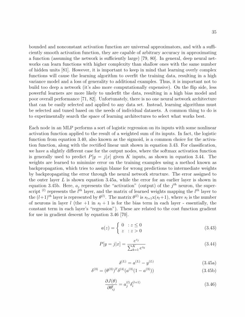
35
bounded and nonconstant activation function are universal approximators, and with a suffi-ciently smooth activation function, they are capable of arbitrary accuracy in approximatinga function (assuming the network is sufficiently large) [79, 80]. In general, deep neural net-works can learn functions with higher complexity than shallow ones with the same numberof hidden units [81]. However, it is important to keep in mind that learning overly complexfunctions will cause the learning algorithm to overfit the training data, resulting in a highvariance model and a loss of generality to additional examples. Thus, it is important not tobuild too deep a network (it’s also more computationally expensive). On the flip side, lesspowerful learners are more likely to underfit the data, resulting in a high bias model andpoor overall performance [71, 82]. Unfortunately, there is no one neural network architecturethat can be easily selected and applied to any data set. Instead, learning algorithms mustbe selected and tuned based on the needs of individual datasets. A common thing to do isto experimentally search the space of learning architectures to select what works best.
Each node in an MLP performs a sort of logistic regression on its inputs with some nonlinearactivation function applied to the result of a weighted sum of its inputs. In fact, the logisticfunction from equation 3.40, also known as the sigmoid, is a common choice for the activa-tion function, along with the rectified linear unit shown in equation 3.43. For classification,we have a slightly different case for the output nodes, where the softmax activation functionis generally used to predict P [y = j|x] given K inputs, as shown in equation 3.44. Theweights are learned to minimize error on the training examples using a method known asbackpropagation, which tries to assign blame for wrong predictions to intermediate weightsby backpropagating the error through the neural network structure. The error assigned tothe outer layer L is shown equation 3.45a, while the error for an earlier layer is shown inequation 3.45b. Here, aj represents the “activation” (output) of the jth neuron, the super-script (l) represents the lth layer, and the matrix of learned weights mapping the lth layer tothe (l+1)th layer is represented by θ(l). The matrix θ(l) is sl+1x(sl+1), where sl is the numberof neurons in layer l (the +1 in sl + 1 is for the bias term in each layer - essentially, theconstant term in each layer’s “regression”). These are related to the cost function gradientfor use in gradient descent by equation 3.46 [70].
a(z) =
0 : z ≤ 0z : z > 0
(3.43)
P [y = j|x] =ezj∑Kk=1 e
zk(3.44)
δ(L) = a(L) − y(L) (3.45a)
δ(3) = (θ(3))T δ(4)(a(3)(1− a(3))) (3.45b)
∂J(θ)
∂θlij= a
(l)j δ
(l+1)i (3.46)

36
Figure 3.12: This shows an example of an MLP architecture neural network.
Many machine learning algorithms are built for classifying binary cases (eg, SVM). To over-come this, the strategy one versus rest is commonly used. The one versus rest strategyemploys one classifier per class, which fits that class against all the other classes. The classwith the highest probability over all other classes is chosen as the predicted class. Advantagesof this method include computational efficiency (only nc classifiers are needed) and inter-pretability (it is possible to gain knowledge about any class by inspecting its correspondingclassifier) [83, 70].
3.7 Feature Selection
No machine learning algorithm can work without good features providing the necessary in-formation for classification. However, even if a dataset contains good features, it is importantto do some analysis to ensure that all features passed to a learning algorithm are relevant6.Passing extraneous features to an algorithm increases computational complexity and thelikelihood of getting stuck in a local optimum rather than the global optimum. Additionally,it has been shown that using only a small subset of relevant features significantly reduces thenecessary number of data points to guarantee good generalization for the learned function[84]. Of the used features, it is often beneficial to avoid repeating information with twohighly similar features, especially for neural network classifiers [71].
There are three different types of feature selection algorithms - wrapper, embedded, and
6A feature xi is often described as a strongly relevant feature if two examples with non-zero probabilityfrom different classes differ only in their assignment to xi. A feature xi is referred to as weakly relevant if itis possible to remove a subset of features such that xi becomes strongly relevant.

37
filter methods. Wrapper methods search the feature space by repeatedly training and test-ing the algorithm on different subsets of features. Depending on the size of the feature space,there are different approaches that can be taken. In general, testing all possible combina-tions of features would be intractable since that would be 2f possible combinations (for fdifferent features). Thus, heuristic methods such as greedy algorithms7 must be used. Anexample would be a forward search (start with 0 features and add a feature each time) wherean added feature is kept if it increases the algorithm’s performance and discarded otherwise.Since this method tests the features directly on the algorithm, it often gives the best perfor-mance for any specific algorithm; however, it is also the most computationally intensive sincethe full algorithm is trained and tested at each step. Embedded feature selection embedsthe feature selection in the learning algorithm itself. For example, weight pruning can bedone to essentially eliminate features that are given sufficiently low weights by the learningalgorithm. The third method, filtering, is generally the cheapest method computationally.Filter methods apply some sort of statistical test or criteria to the features. These methodsare more general than wrapper or embedded methods, so they generally give slightly worseperformance for a specific learning algorithm. Thus, they are generally done to provide afeature ranking or subset to be passed to a wrapper or embedded method to reduce thesearch space and computational demand [84].
7A greedy algorithm attempts to search a space by making a locally optimal decision at each step.

Chapter 4
Process
4.1 Equipment and Setup
The idea behind this thesis is to identify the node that is sending a message and comparethis with known information about which node(s) should be sending this message (ie, is itthat ECUs job to control this feature or provide this information). Since the purpose ofthe message is contained in the message identifier, an experiment was conducted to see ifa node could be recognized from the way it sends a specific identifier. This way, the un-derlying message content of the signals being compared is always the same, and it can bedetermined if the proper node is sending a message from the content in the message identifier.
For this thesis, a 3 node CAN bus constructed from Maxon EPOS2 50/5 positioning con-trollers (part number 347717) was used to generate data for testing. This bus uses theCANopen protocol, so each node has a configurable four-bit identifier associated with it thatis part of the CAN message identifier. For the data collection, data relevant to each nodesending the identifier of interest was collected one at a time. In other words, at any point ofdata collection, one node on the bus had the given identifier, and all messages of the sametype with the same full CAN message identifier were kept for processing. The measurementswere made using the external CAN connector holes that are on each node.
A Picoscope 5442A from Picotech was used to collect data on the bus from both the CANHand CANL using two (simultaneous) channels. The wiring diagram of this set-up is shown inFigure 4.1. This figure shows the Picoscope attached to an external CAN connector on node1, where it was plugged in for most of the data collection. However, as will be described insection 4.2, some data was also collected with the Picoscope plugged into the available CANconnector on node 3. Additionally, between some collections, the Picoscope was unpluggedand plugged back in to the CAN connector, but the same P6060 probes, which came withthe Picoscope, were used for all data collection. The wiring of the CAN lines was left alone,
38
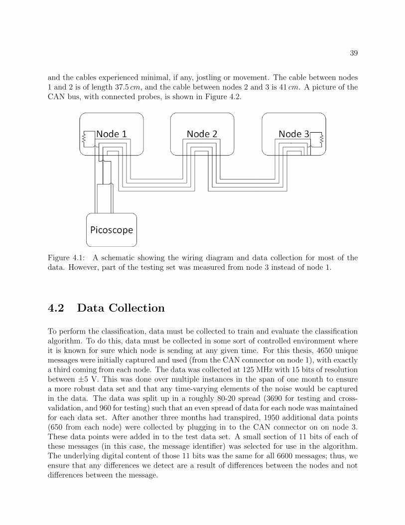
39
and the cables experienced minimal, if any, jostling or movement. The cable between nodes1 and 2 is of length 37.5 cm, and the cable between nodes 2 and 3 is 41 cm. A picture of theCAN bus, with connected probes, is shown in Figure 4.2.
Figure 4.1: A schematic showing the wiring diagram and data collection for most of thedata. However, part of the testing set was measured from node 3 instead of node 1.
4.2 Data Collection
To perform the classification, data must be collected to train and evaluate the classificationalgorithm. To do this, data must be collected in some sort of controlled environment whereit is known for sure which node is sending at any given time. For this thesis, 4650 uniquemessages were initially captured and used (from the CAN connector on node 1), with exactlya third coming from each node. The data was collected at 125 MHz with 15 bits of resolutionbetween ±5 V. This was done over multiple instances in the span of one month to ensurea more robust data set and that any time-varying elements of the noise would be capturedin the data. The data was split up in a roughly 80-20 spread (3690 for testing and cross-validation, and 960 for testing) such that an even spread of data for each node was maintainedfor each data set. After another three months had transpired, 1950 additional data points(650 from each node) were collected by plugging in to the CAN connector on on node 3.These data points were added in to the test data set. A small section of 11 bits of each ofthese messages (in this case, the message identifier) was selected for use in the algorithm.The underlying digital content of those 11 bits was the same for all 6600 messages; thus, weensure that any differences we detect are a result of differences between the nodes and notdifferences between the message.

40
Figure 4.2: A picture of the CAN bus is shown here. The Picoscope probes in this pictureare attached to node 3 in the top right.
4.3 Preprocessing and Feature Extractions
Once the data has been collected, preprocessing must be applied to the data before classifi-cation can be performed. This section will go through all of the preprocessing that is doneon the data before extracting any features, as well as the features that were extracted.
The first step in the preprocessing is to read the bits of the message to find the appro-priate section to use for the classification. Additionally, for a real-time implementation, thiswould also be necessary for identifying the message and determining expected sources. Oncethis has been identified, features that require the original signal are extracted. These arethe average bit length, average rising edge derivative, and average falling edge derivative.To extract the average bit length, the signal is broken up according to where bit edges are.Then, the time length of the flat areas are divided by the theoretical bit times for 1 Mbit/s

41
(1µs) to get a ‘time per bit’. These values are then averaged to get the overall average bitlength for the signal. For the rising and falling edge derivatives, the first and last valuesdetected to be a part of the edge are used. The derivative is taken to be the voltage differenceover the time difference for these two points (∆V
∆t). This is done separately for each line.
The next step is to separate the signal into 2 components - a pure signal component and anoise component. To do this, the CANH and CANL lines are tracked using a simple Schmitttrigger technique, and a noiseless copy of each signal is constructed using the theoreticalvoltage values for high and low bits on each line (CANH and CANL). For the bit edges, thenoiseless signal simply follows the voltages exactly since it is difficult to split this up intosignal and noise components. Once this noiseless copy of the signal has been constructed,the final ‘signal’ and ‘noiseless signal’ are defined to be the difference between the CANHand CANL lines in order to take advantage of the common mode rejection of the CAN busarchitecture. The noise component is then found to be the difference of the noisy and noise-less signals. An example of the resulting noise component is shown in Figure 4.3.
Figure 4.3: An example of the noise measured in one of the CAN bus nodes used for thisthesis.
With the noise component separated, the rest of the features can be extracted from thenoise. The entirety of the extracted features are summarized with brief descriptions in Ta-ble 4.1. These features and reasons for choosing them were discussed in Chapter 3. Theorder for the autoregressive model was determined by fitting models of order 1 through 25

42
to the samples in the testing data set, and the best order was selected based on Akaike’sinformation criterion.
4.4 Feature Selection
For the feature selection, a combination of filter and wrapper methods were used. The fea-tures were ranked based on a custom scoring method, and then a simple forward search wasperformed using the top performing features.
The feature ranking was performed based on performance from two statistical tests: the inde-pendent samples t-test, and the Kolmogorov-Smirnov test. The independent samples t-testis chosen because it is an often used location test with good statistical power1 for normallydistributed data and is the preferred test for analysis of variance. The Kolmogorov-Smirnovtest was chosen because it makes virtually no assumptions, meaning that it should be reliablefor almost any data, and the author believes that its test statistic is a crucial requirementfor data classification since a large difference between two cdfs indicates good separabilityof the data, which makes classification easier. Since it is desired that each class populationbe different from all other populations, a multiple comparison methods is used, and p-valuesfrom different tests are summed since each value is already on the same scale (p ∈ [0, 1]).Furthermore, since consistent classification performance requires consistent data, the dataset is split in half, and each class is also compared with itself. The multiple comparison scoreis found according to equation 4.1, where ti,j is the p-value from a t-test comparing class iwith class j, and ki,j is the p-value from the same Kolmogorov-Smirnov test. Thus, a highscore represents a feature with a population that is both consistent within its class and dif-ferent between classes. However, since many machine learning algorithms, including SVMs,naturally perform binary classification and are typically extended to multiclass classificationthrough one-versus-rest methods, a one-versus-rest scoring system was also developed, andits scoring function is shown in equation 4.2, where ti,iC represents the p-value from a t-testbetween the data for class i and all data not in class i. Additionally, since highly correlatedfeatures likely don’t provide significant new information, the feature ranking is kept frombecoming clogged up with similar features by implementing a correlation check. After eachfeature is scored, the correlation matrix for the feature matrix is calculated. When twofeatures are found to have correlation ρ > 0.9, the higher-scoring feature is kept, and thescore of the lower-scoring feature is set to 0.
score =
∑ni=1(ti,i + ki,i)∑n−1
i=1
∑nj=i+1(ti,j + ki,j)
(4.1)
1Statistical power represents the probability of correctly rejecting the null hypothesis when the alternativehypothesis is true.

43
FFT This is a frequency estimate made purely by takingthe FFT of the data with a Chebyshev window (α =4.5)
Welch Spectral Density Estimate This is a frequency estimate made using Welch’smethod with a Hamming window.
Autoregressive spectral estimate An estimate of the spectral content of a signal doneby constructing a 12th order autoregressive model.This method assumes a nondeterministic, weaklystationary signal.
db2 detail coefficients The detail coefficients from a single layer dis-crete wavelet decomposition using Debauchies 4 tapwavelet. The detail coefficients come from the con-volution of the wavelet function with the data.
db2 approximation coefficients The approximation coefficients from a single layerdiscrete wavelet decomposition using Debauchies 4tap wavelet. The approximation coefficients comefrom the convolution of the scale function with thedata.
time-reversal asymmetry statistic The time-reversal asymmetry statistics for lags 1-5are extracted. This measure is similar to a skewnessmeasure for the lagged differential signal.
autocovariance The autocovariance of the data for all lags is calcu-lated.
average rising edge derivative The average derivative of a rising edge in the signal.average falling edge derivative The average derivative of a falling edge in the signal.average bit length The average length of 1 bit of a signal in the message.noise variance The variance of the noise estimate for the signal.absolute sum of difference The sum of the absolute value of the difference be-
tween successive noise values.percentage of increasing difference The percentage of positive values in the vector of
differences between successive noise values.
Table 4.1: This table includes all the features extracted for analysis by the algorithm.
44
score =
∑ni=1(ti,i + ki,i)∑n
i=1(ti,iC + ki,iC )(4.2)
With this feature ranking, simple forward searches are used to perform the final featureselection for each machine learning algorithm. Each algorithm is initially run only on thehighest performing feature, and then features are added one at a time in order of performance,and the algorithm is again run on each new feature set. A five-fold cross validation scheme isused, and the algorithm’s performance is measured according to its average performance onthe cross-validation dataset, as measured by the log-loss cost function. The first feature isselected if it can provide greater than 33% classification (in other words, better classificationthan random guessing), and subsequent features are selected if the loss function decreases.Selected features are kept in the feature set, while features not meeting this criteria arediscarded from the selection process. This is iteratively done to test the top 100 scroringfeatures from each algorithm. First, the top 100 features from the multiple comparisonmethod are used (in order from highest to lowest scoring), since this method gives thefeatures which are most different between each class. Then, the top 100 features from theone-versus-rest scoring method are passed to the search since this method is more likelyto give features which have some similar classes, but at least one class that is significantlydifferent from the other two (which will help with classification of data coming from saidclass).
4.5 Classification
There are many algorithms which can be used to perform the classification, as discussed inChapter 3. This thesis picks two of the more popular and powerful algorithms, which arethe support vector machine (SVM) - as implemented in scikit-learn [85] - and multilayerperceptron (MLP) neural network - as implemented in Keras [86]. The SVM is chosen be-cause it guarantees to find the globally optimum solution according to its parameters andit is resistant to overfitting, while the MLP is chosen for its ability to learn more complexfunctions. Both of these algorithms are tested (including separate feature selection), and theresults can be compared.
Each algorithm has some hyperparameters that must be tuned. This tuning is done ini-tially with the ten highest ranking features from the feature filtering method to get ap-proximate solution, and another grid search is performed on the final feature set to ensurebest performance. To tune these parameters, a grid search with five-fold cross validation isimplemented using scikit-learn’s API [85]. For the SVM, the parameters tuned include theerror penalty C for the cost function (essentially an inverse regularization coefficient) andthe kernel. Additionally, since some kernels themselves have hyperparameters (the degree ofthe polynomial and γ = 1
2σ2 for the gaussian kernel), these are included in the search. Thevalues searched are shown in table 4.2. For the MLP, the optimization algorithm, amount of

45
C 0.25, 0.5, 1.0, 1.5, 2.0, 2.5, 3.3, 5.0kernel function polynomial and gaussianpolynomial degree 2, 3, 4, 5γ 0.025, 0.05, 0.075, 0.10, 0.15, 0.20, 0.25, 0.33, 0.4, 0.5,
0.67, 0.75, 0.9, 1.0
Table 4.2: A table containing the values used for the grid search to determine the bestvalues for the hyperparameters of the SVM.
neurons in layers 1 and 2 (64, 32), (32, 32), (64, 64), (32, 64), (48, 32), (48, 48),(32, 48)
optimization algorithm stochastic gradient descent, adam, adamax, adagrad,adadelta, nadam, RMSprop
dropout 0.4, 0.5, 0.6batch size 8, 16, 32training epochs 10, 25, 50
Table 4.3: A table containing the values used for the grid search to determine the bestvalues for the hyperparameters of the MLP.
dropout, activation function, number of neurons per layer, number of training epochs, andbatch size are are included in the grid search. The values for these are shown in table 4.3.

Chapter 5
Results
5.1 Feature Extraction
In this section, the examples of measured noise shown in Figure 4.3, will be used to showexample results of each feature extraction outlined in section 4.3 will be shown.
The autocovariance of the signals are claculated and plotted in Figure 5.1. It does seemto smooth ot the noise some, but differences between the nodes are not obvious, and nofeatures from the autocovariance are chosen.
The Chebyshev-windowed FFT is taken and shown in Figure 5.2. As it can be seen, thereis quite a bit of noise in the estimate. Thus, while it looks by eye like there may be somepoints of differences in the estimate, it is desirable to find an estimate with less noise.
Welch’s spectral estimate is calculated and shown in Figure 5.3. Again, the estimate isquite noisy. From this, it was hypothesized that, in order to get an estimate which was lessnoisy, a different approach would need to be taken.
The autoregressive spectral estimate is then calculated. The autoregressive order is found byfitting autoregressive models of order 1− 25 to each of the training samples, and the best fitis determined using Akaike’s information criteria. The average value of these best fit ordersis taken, and found to be 12. The resulting spectral estimate is shown in Figure 5.4, and theautoregressive model fits for each node are overlayed with the noise data in Figures 5.5, 5.6,and 5.7 to demonstrate model fit. It can be seen that it follows a similar underlying patternas the FFT, but it provides a significantly smoother representation since it is based only onthe coefficients of a 12th order autoregressive model.
The wavelet transformations are calculated using Daubechies 4 tap wavelet. The resulting
46

47
Figure 5.1: This plot shows an example of the calculated frequency spectrum from theChebyshev-windowed FFT.
Figure 5.2: This plot shows an example of the calculated frequency spectrum from theChebyshev-windowed FFT.

48
Figure 5.3: This plot shows an example of the calculated Welch estimate of the frequencyspectrum.
Figure 5.4: This plot shows an example of the calculated frequency spectrum from autore-gressive model.

49
Figure 5.5: This plot shows the autoregressive fit for the noise sample for node 1.
Figure 5.6: This plot shows the autoregressive fit for the noise sample for node 2.
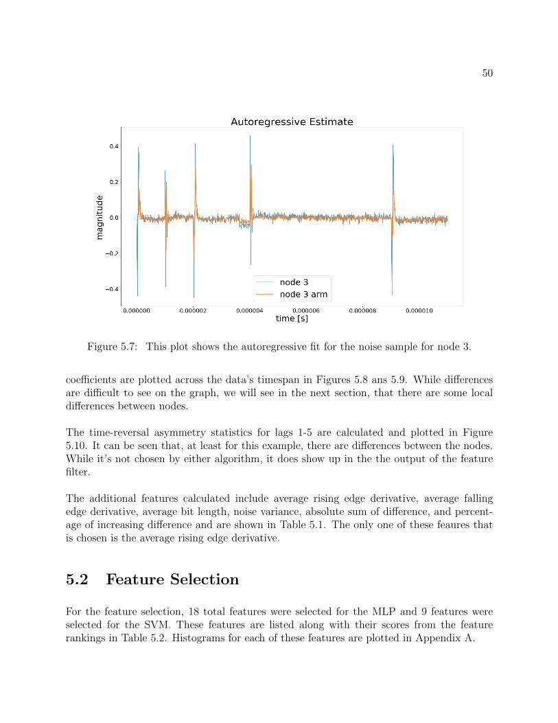
50
Figure 5.7: This plot shows the autoregressive fit for the noise sample for node 3.
coefficients are plotted across the data’s timespan in Figures 5.8 ans 5.9. While differencesare difficult to see on the graph, we will see in the next section, that there are some localdifferences between nodes.
The time-reversal asymmetry statistics for lags 1-5 are calculated and plotted in Figure5.10. It can be seen that, at least for this example, there are differences between the nodes.While it’s not chosen by either algorithm, it does show up in the the output of the featurefilter.
The additional features calculated include average rising edge derivative, average fallingedge derivative, average bit length, noise variance, absolute sum of difference, and percent-age of increasing difference and are shown in Table 5.1. The only one of these feaures thatis chosen is the average rising edge derivative.
5.2 Feature Selection
For the feature selection, 18 total features were selected for the MLP and 9 features wereselected for the SVM. These features are listed along with their scores from the featurerankings in Table 5.2. Histograms for each of these features are plotted in Appendix A.

51
Figure 5.8: This plot shows the calculated detail coefficients for the sample noise.
Figure 5.9: This plot shows the calculated approximation coefficients for the sample noise.
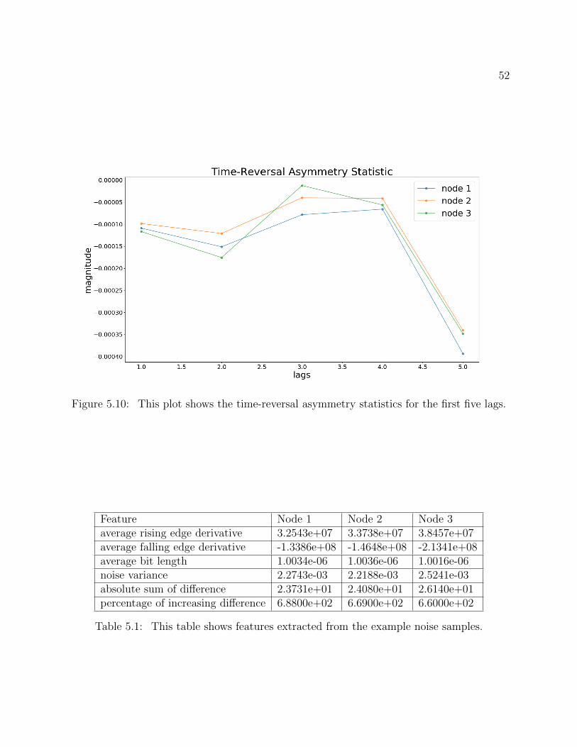
52
Figure 5.10: This plot shows the time-reversal asymmetry statistics for the first five lags.
Feature Node 1 Node 2 Node 3average rising edge derivative 3.2543e+07 3.3738e+07 3.8457e+07average falling edge derivative -1.3386e+08 -1.4648e+08 -2.1341e+08average bit length 1.0034e-06 1.0036e-06 1.0016e-06noise variance 2.2743e-03 2.2188e-03 2.5241e-03absolute sum of difference 2.3731e+01 2.4080e+01 2.6140e+01percentage of increasing difference 6.8800e+02 6.6900e+02 6.6000e+02
Table 5.1: This table shows features extracted from the example noise samples.

53
Feature Algorithms MC Ranking OVR RankingAutoregressive PSD 14.28 MHz SVM and MLP 1 4301
db2 approximation coefficient for t = 4.096µs SVM and MLP 3 353Autoregressive PSD 17.15 MHz MLP 4 4682FFT magnitude for 12.08 MHz MLP 9 730FFT magnitude for 13.06 MHz MLP 10 634FFT magnitude for 11.05 MHz MLP 13 736FFT magnitude for 12.51 MHz SVM and MLP 16 174FFT magnitude for 18.01 MHz MLP 17 4401
db2 approximation coefficient for t = 1.088µs SVM and MLP 4405 4FFT magnitude for 11.96 MHz MLP 613 8FFT magnitude for 1.831 MHz MLP 238 10FFT magnitude for 10.99 MHz MLP 1120 12
db2 approximation coefficient for t = 2.240µs MLP 3987 18FFT magnitude for 2.075 MHz MLP 118 21FFT magnitude for 11.90 MHz MLP 182 22FFT magnitude for 13.37 MHz MLP 524 23FFT magnitude for 10.31 MHz MLP 678 37FFT magnitude for 11.84 MHz MLP 448 39
Time-reversal asymmetry statistic for lag 4 SVM 175 1FFT magnitude for 2.197 MHz SVM 212 6FFT magnitude for 12.82 MHz SVM 522 18FFT magnitude for 21.06 MHz SVM 408 84
Table 5.2: This table includes all the features used by either algorithm. The ranking byeach filter algorithm is also shown (MC Ranking stands for multiple comparison ranking andOVR Ranking stands for one-versus-rest ranking).

54
5.3 Classification
The best accuracy achieved by the MLP is 99.9% accuracy on the test data set, while theSVM maxes out at 99.8%. Graphs of the classification accuracy versus number of featuresare shown in Figures 5.12 and 5.11 for the MLP and SVM, respectively, and the confusionmatrices for each are shown in Tables 5.3 and 5.4. The parameters used for each of thesemodels are the parameters found to be best from the grid search mentioned in Chapter 4.For the SVM, these are: a gaussian kernel function with γ = 0.075 and a penalty parameterof C = 5 for the error term in the optimization function. For the MLP, these are: 3 layers(plus the input layer) with 64, 32, and 3 (for three classes) neurons, respectively; the Adamoptimization method [87]; a dropout of 0.5 for the first 2 layers; the rectified linear activa-tion function for the first two layers (with softmax activation for the classification layer); 50epochs for training; and a batch size of 32.
Figure 5.11: A plot showing how the accuracy of the SVM changes as features are added(only including those features chosen as the final feature set for the SVM).
However, as it can be seen from the above plots, classification accuracies in the high 90%are acheived by both algorithms after only 2 features. Thus, if desired, the algorithms couldbe constructed using only 2 features to save on computation. To find the best set of twofeatures, an exhaustive search was done for each algorithm over all combinations of 2 fea-tures from the features in Table 5.2. The feature set with the lowest log loss from a five-foldcross validation was selected. This resulted in a reasonably wide spread of log loss values,including some pretty high losses. The best combination of 2 features ended up being the

55
Figure 5.12: A plot showing how the accuracy of the MLP changes as features are added(only including those features chosen as the final feature set for the MLP).
Predicted TotalNode 1 Node 2 Node 3
Act
ual Node 1 860 0 0 860
Node 2 0 855 5 860Node 3 0 0 860 860
Table 5.3: Confusion matrix for the best SVM configuration
Predicted TotalNode 1 Node 2 Node 3
Act
ual Node 1 860 0 0 860Node 2 0 859 1 860Node 3 0 1 859 860
Table 5.4: Confusion matrix for the best MLP configuration
same for both algorithms - the AR Spectral Magnitude at 14.28 MHz and the approximationcoefficient from the db2 wavelet transform corresponding to t=4.096 µs from the convolu-tion. In this case, the SVM achieved the best accuracy on the test data set, at 99.2%, while
56
the MLP only reached 98.3%.
5.4 Additional Testing
In order to investigate a potential cause for the discrepancy between the characteristics ofthe signals for each node, data was taken from a different point on the bus, testing for anydependency for measurement location. However, the relevant features showed no verifiablechange according to statistical tests. In fact, the best MLP still achieved 99.9% accuracy onthis data set, and the SVM still achieved 99.8% accuracy, illustrating that this change did notnoticeably affect the performance of the classification. Despite this, it is important to realizethat the CANH and CANL lines are not perfect conductors, but have impedances whichmust be taken into account when designing a system. Therefore, it is best practice to ensurethat training data is sampled from the same point on the bus as the final implementation.

Chapter 6
Discussion and Conclusions
6.1 Discussion of practical application
6.1.1 False Alarm Probability
Since 100% identification accuracy is not quite achieved in this paper, and it can certainlynever be guaranteed for new data, the possibility of misclassifications must be taken intoaccount. These misclassifications give the potential for false alarm intrusion detections. Forthe sake of this discussion, we will consider an algorithm with 99.7% accuracy over thelong run. While this seems like an extremely high accuracy, at this accuracy we surpass50% probability of a misidentification after only 167 messages, which can be sent in a smallamount of time on the CAN bus. Therefore, the node identification would likely need to becombined with an additional layer. Here, we will propose a strikes-based approach, whichkeeps a memory of a certain number of previous messages and doesn’t raise a flag until acertain number of strikes have been reached within its memory.
It has been found that 0.5 milliseconds is a reasonable average spacing between messages[22]. Thus, we might expect around 2,000 messages per second in a CAN bus. We mustnow decide a number of messages to keep in memory based on an average span of time thatis acceptable to allow a potential hacker to control the bus and a percentage of allowableperceived ‘rogue’ messages within that span of time. The tradeoff here is that as we decreasethe number of messages, we must increase the percentage of allowable ‘rogue’ messages toprevent the false alarm probability from increasing. To select these parameters, we refer tothe binomial distribution. Assuming the correctness of each message is independent, we canmodel the number of misidentifications k in a span of n messages with a binomial distribu-tion. Then, the false alarm probability will be 1 − P [k ≤ nq] where q is the percentage ofallowable rogue messages (so nq is the number of rogue messages for a block of n messages).Since P [k ≤ nq] is the cdf of the binomial, this can be calculated using the regularized
57

58
incomplete beta function [88]. This calculation was performed using mpmath for python inorder to achieve the best possible floating point precision [89]. A plot showing the tradeoffbetween time and percentage is shown in Figure 6.1. The false alarm probability 1e − 15is used to estimate about one billion driving-years (one person driving for one year’s worthof time would be one driving-year) before one false alarm can be expected. This numberis believed to be sufficient for an extremely sparse occurrence of false alarms. At this falsealarm rate, we would have to allow up to about 10% of messages to be marked ‘rogue’ in ahalf second interval before we would raise a flag. Alternatively, if we accept more frequentfalse alarms - say, one every 100,000 driving-years, we decrease the false alarm probability to1e− 11. However, it can be seen that we do not get much of a decrease in the allowed roguemessages for the significance of the increase in false alarms. At 0.5 s long message blocks(1000 messages per block), we would only decrease the allowable rogue messages by 0.4%,or 4 messages, and at 0.25 s long message blocks (500 messages per block), we would onlydecrease the allowable rogue messages by 0.8%, or, again, 4 messages.
Figure 6.1: This plot shows how the maximum allowable messages marked as rogue varieswith average time length based on constant false alarm probabilities of 1e− 15 and 1e− 11.
6.1.2 Computational Complexity of Online Implementation
It is important to consider the computational complexity of this algorithm in order to as-sess its real-world usefulness. In this section, we will discuss computational complexities

59
for individual features, as well as an overall computational complexity. For the sake of thisdiscussion, we will assume the use of an MLP neural network since that achieved slightlyhigher maximum performance in this thesis.
Considering all the features used by the MLP gives 18 features, including magnitudes from anFFT, autoregressive power spectral density estimate, discrete wavelet transform, and time-reversal asymmetry statistic. The typical computational complexity of a FFT is O(NlogN);plus, one O(N) computation is required to apply the time-domain window). The full discretewavelet transform is O(WN), where W is the number of coefficients for the wavelet or scalefunction. However, since we again require only a subset of the transform, we can reduce thisto O(W ) computations for each coefficient. Additionally, the db2 wavelet transform usesonly four coefficients each for its scale and wavelet functions, making each of these computa-tions quite small. This leaves us with the calculation for autoregressive PSD estimate, whichis the most computationally demanding computation in this group. To solve this, a numberof steps must be taken. First, the autocovariance must be found, which is an O(N2) compu-tation. However, we can cheat with this computation. Using the property that convolutionin time domain is multiplication in the frequency domain, we can find the autocovarianceusing an FFT, which requires 2 O(NlogN) calculations. Next, the autoregressive coefficientsmust be found, which is an O(M2N) computation, where M is the number of autoregressivecoefficients. An additional O(NlogN) computation must be made to find the PSD estimatebased on these parameters. The dominant computation here is O(M2N), so, technically,this full algorithm is O(M2N); however, for an embedded, real-time application, these othersteps cannot be ignored. Finally, the 3-layer feedforward MLP neural network requires threecomputations of O(K0K1), O(K1K2), and O(K2K3) complexity, where Kl denotes the num-ber of neurons in layer l (and K0 is the number of features).
If we use all features, the total computation required includes 4 O(NlogN), 1 O(M2N),3 O(W ), and 3 O(KlKl−1) computations. This will be dominated by the O(M2N) computa-tion, which, using the data vectors of N = 1, 376 and AR order M = 12 used in this thesis,requires 198, 144 computations. Continuing this, using the time complexities (for K0 = 18,K1 = 64, K2 = 32, and K3 = 3) results in a lower bound estimate of 261, 996 calculations.The vast majority of this (198, 144) comes from the O(M2N) calculation for the autoregres-sive model. Of course, it is also possible to reduce computational time by using only a subsetof these features, such as the top performing set of 2 features, to reduce the computationalload.
6.1.3 Hardware Required for Online Implementation
In order to implement this solution, a few additional pieces of hardware would need to beadded to a CAN bus node. These include an ADC to make analog voltage measurements formeasuring the noise and some sort of processor to be able to handle the feature extraction

60
and classification (the initial feature selection and training of the algorithm can be done of-fline and on separate computers). This section will discuss some suggestions for the selectionof such hardware.
The ADC will need to be selected based on both sample rate as well as resolution. Thesample rate used in this thesis is 125 MHz. The largest frequency directly used in this thesisis the feature containing the power spectral density at 43.58 MHz, so, the frequency couldpotentially be decresed to around 90 MHz, but this is not recommended since sample ratehas a more complicated relationship with the outputs of other feature extraction techniques,such as the wavelet transformation. Thus, a minimum of 125 MHz is suggested. Addition-ally, the ADC should be at least 14 bits to give the equivalent of the ADC used in this thesis(15 bits over (−5, 5)V , or, basically, 14 bits over (0, 5)V since negative voltage is neverused). However, more bits can only assist in obtaining the best data, and it is recommendedto get an ADC with as many bits as possible. Additionally, since transition information isnot used in the final results of this thesis, there has been some discussion about optimizingthe range of the ADC to only contain the areas around the high and low voltage values. Thiscould be done by using two separate ADCs with tight ranges set around the high and lowvoltages, and a voltage-controlled switch could be used to control which ADC is read by theprocessor. This could be a good topic for future work.
The processing power to analyze a 125 MHz data stream in real-time is significant. Thepotential for the use of a DSP chip will be discussed here, but an application-specific inte-grated circuit (ASIC) or field-programmable gate array (FPGA) could also be designed toachieve high-performance parallel processing. For determining the necessary specificationsof a DSP, we will analyze the number of operations necessary for a full 11-bit section of data(since the section used for classification in this thesis is 11 bits long). We will assert that,if implemented on the identifier frame in a CAN message, the processing must be done bythe end of the data frame, which is traditionally 8 bytes long in car communications, givingapproximately 64µs for the calculations (assuming a 1Mbit/s bitrate and no stuffed bits,which, if present, would increase the allowable time). Based on our lower bound computa-tional estimate from 6.1.2, allowing for that we ignored some constant factors, and buildingin some additional room for overhead, we will require the capability for at least 600, 000 cal-culations in this 53µs time span. As an example, the TMS320C6678 from TI [90], availablefor roughly $190, has 8 cores running at 1.25 GHz, making it capable of 640, 000 operationsduring this time frame and thus meeting this criteria. If necessary, the allowed processingtime could be extended to include the 16-bit CRC frame, giving an additional 16µs for thecalculation. For comparison, in this amount of time, the TMS320C6678 is capable of 800, 000operations during this time frame.

61
6.1.4 Portability
This thesis has demonstrated results for only one CAN bus. However, it is believed that itwill be portable to other CAN buses because of the amount of features extracted. While allthe same features will likely not be significant for all CAN buses, it is believed that all willhave some set of features which can be used to perform a classification, and this algorithm isset up so that a large number of features can be extracted, and the best will be chosen basedon the data. Additionally, if desired, more features can easily be added without makingsignificant changes to the overall algorithm. Additional wavelets and PSD estimates areobvious potential candidates for addition, as well as making use of existing feature extractionlibraries such as tsfresh [91] and the highly comparitive time series analysis introduced in[66] and [67].
6.2 Review
6.2.1 Summary
As cars become more complex, they are including more and more ECUs with much morepower and connectedness with the world. While this makes for a publicly better product,it also comes with the need for improved security. It has been demostrated that cars canbe hacked into remotely and, once control of the CAN bus has been achieved, a car can becontrolled to act as desired or display false warnings to the driver.
This thesis presents a method for assisting in intrusion detection on a CAN bus. We havepresented a method of “fingerprinting” the transceivers on the CAN bus, which provides anassurance for which node is sending a message. By identifying the nodes on the CAN bus,it becomes easier to evaluate traffic on the bus and detect suspicious activity.
6.2.2 Accomplishments
The classification of 3 nodes on a CAN bus was tested on an independent data set, andaccuracy as high as 99.9% using as little as 13 features with an MLP neural network. Ad-ditionally, a potential path for avoiding false alarms has been given. This thesis provides agood proof of concept of the proposed algorithm, and will hopefully be an impetus for futurework in this area.

62
6.2.3 Future Work
To further verify this algorithm, it is necessary to implement it on more CAN buses to provethat it is effective. This includes testing on CAN buses with more than 3 nodes since cars willtypically have many more ECUs. If it is necessary to improve performance, more featurescan be added, as discussed in 6.1.4 or an ADC with higher resolution and/or sampling ratecan be used.
It would also be helpful for more testing to be done in which certain parameters relatedto the CAN bus were varied to see how much each parameter effects the measurementsbeing made and subsequent classification. For example, changing the cable lengths on theCAN bus and taking more data would test how much of the captured effect is coming fromtransmission line effect, and artificially removing the large spikes in the noise measurementswould test how much of the measured effect is a result of the asynchronicity between theswitching transistors driving the CANL and CANH lines in the node transceiver.
An additional area of great interest would be to improve the measurement of timing charac-teristics on the CAN bus. It is known and well understood that any oscillator on a CAN busnode will have manufacturing tolerances around a certain frequency. Such tolerances shouldlead to differences between the internal frequencies of each node and result in a useful figurefor classification. This could be done by using a time-to-digital converter to obtain bettertime resolution.
Once this algorithm has been verified to work on several CAN buses, a true online im-plementation must be developed and tested. This requires selecting the proper hardwarecomponenets, developing the integration of these components with the existing componentson a CAN bus, writing the feature extraction and classification to work in real time, anddeveloping the protocol for when to become suspicious and what to do if it is believed thatan attack is occurring. One way to do this would be to develop a way to integrate theknowledge provided by the node identification into existing intrusion detection systems.
6.2.4 Final Remarks
This thesis presents a promising method for identifying devices on a communication bus.While this work focused mainly on the CAN bus, such identification has obvious securitybenefits for any communication bus. Knowing the origin of a message can identify both theaddition of new units to the bus, as well as compromised units that are attempting to takecontrol of functionality for malicious purposes.

Bibliography
[1] Charlie Miller and Chris Valasek. Adventures in Automotive Networks and ControlUnits. Tech. rep. IOActive, 2014. url: https://ioactive.com/pdfs/IOActive_Adventures_in_Automotive_Networks_and_Control_Units.pdf (visited on 10/20/2017).
[2] CANHack.org - Index page. url: https://canhack.org/board/ (visited on 12/02/2017).
[3] Craig Smith. Car Hacking 101: Tools of the Trade — Make: Apr. 2016. url: https://makezine.com/2016/04/08/car-hacking-tools-trade/ (visited on 11/01/2017).
[4] Ariel Nunez. An Introduction to the CAN Bus: How to Programmatically Control aCar. June 2017. url: https://news.voyage.auto/an-introduction-to-the-can-bus-how-to-programmatically-control-a-car-f1b18be4f377 (visited on11/01/2017).
[5] Andy Greenburg. A $60 Gadget That Makes Car Hacking Far Easier. Mar. 2015. url:https://www.wired.com/2015/03/60- gadget- thatll- make- car- hacking-
easier-ever/ (visited on 11/01/2017).
[6] Kristoffer Smith. a complete guide to hacking your vehicle bus on the cheap & easy - part1 (hardware interface). Mar. 2013. url: https://theksmith.com/software/hack-vehicle-bus-cheap-easy-part-1/ (visited on 11/01/2017).
[7] Eric Evenchick. CAN Hacking: Introductions. Oct. 2013. url: https://hackaday.com/2013/10/21/can-hacking-introductions/ (visited on 11/01/2017).
[8] Hack Your Vehicle CAN-BUS With Arduino and Seeed CAN-BUS Shield. url: http://www.instructables.com/id/Hack-your-vehicle-CAN-BUS-with-Arduino-and-
Seeed-C/ (visited on 11/01/2017).
[9] Pierluigi Paganini. Car Hacking: You Cannot Have Safety without Security. Feb. 2014.url: http://resources.infosecinstitute.com/car-hacking-safety-without-security/ (visited on 11/01/2017).
[10] Chad Gibbons. Chad Gibbons’ Blog. url: http://chadgibbons.com/ (visited on11/01/2017).
[11] Car Hacker′s Handbook by Craig Smith – CanBusHack. url: http://canbushack.com/product/car-hackers-handbook-by-craig-smith/ (visited on 11/01/2017).
63
BIBLIOGRAPHY 64
[12] Blog – CanBusHack. url: http://canbushack.com/blog/ (visited on 11/01/2017).
[13] Edward Markey. S.1806 - 114th Congress (2015-2016): SPY Car Act of 2015. eng.webpage. July 2015. url: https://www.congress.gov/bill/114th- congress/
senate-bill/1806/all-info (visited on 10/11/2017).
[14] Stephen Checkoway et al. “Comprehensive Experimental Analyses of Automotive At-tack Surfaces.” In: USENIX Security Symposium. San Francisco, 2011. url: http://static.usenix.org/events/sec11/tech/full_papers/Checkoway.pdf (visitedon 09/08/2017).
[15] Charlie Miller and Chris Valasek. “A survey of remote automotive attack surfaces”.In: Black Hat USA 2014 (2014).
[16] Charlie Miller and Chris Valasek. “Remote exploitation of an unaltered passengervehicle”. In: Black Hat USA 2015 (2015). url: https://securityzap.com/files/Remote%20Car%20Hacking.pdf (visited on 09/08/2017).
[17] Charlie Miller and Chris Valasek. CAN Message Injection. June 2016. url: http:
//illmatics.com/can%20message%20injection.pdf (visited on 10/23/2017).
[18] Rebecca Bace and Peter M. Mell. “Intrusion Detection Systems”. en. In: Special Publi-cation (NIST SP) - 800-31 (Nov. 2001). doi: 151244. url: https://www.nist.gov/publications/intrusion-detection-systems (visited on 10/19/2017).
[19] Hung-Jen Liao et al. “Intrusion detection system: A comprehensive review”. In: Journalof Network and Computer Applications 36.1 (Jan. 2013), pp. 16–24. issn: 1084-8045.doi: 10.1016/j.jnca.2012.09.004. url: http://www.sciencedirect.com/
science/article/pii/S1084804512001944 (visited on 10/11/2017).
[20] Tobias Hoppe, Stefan Kiltz, and Jana Dittmann. “Security threats to automotive CANnetworks—Practical examples and selected short-term countermeasures”. In: Reliabil-ity Engineering & System Safety. Special Issue on Safecomp 2008 96.1 (Jan. 2011),pp. 11–25. issn: 0951-8320. doi: 10 . 1016 / j . ress . 2010 . 06 . 026. url: http :
//www.sciencedirect.com/science/article/pii/S0951832010001602 (visitedon 10/11/2017).
[21] A. Taylor, N. Japkowicz, and S. Leblanc. “Frequency-based anomaly detection forthe automotive CAN bus”. In: 2015 World Congress on Industrial Control SystemsSecurity (WCICSS). Dec. 2015, pp. 45–49. doi: 10.1109/WCICSS.2015.7420322.
[22] H. M. Song, H. R. Kim, and H. K. Kim. “Intrusion detection system based on theanalysis of time intervals of CAN messages for in-vehicle network”. In: 2016 Inter-national Conference on Information Networking (ICOIN). Jan. 2016, pp. 63–68. doi:10.1109/ICOIN.2016.7427089.
[23] Marko Wolf and Timo Gendrullis. “Design, Implementation, and Evaluation of a Ve-hicular Hardware Security Module.” In: ICISC. Springer, 2011, pp. 302–318.
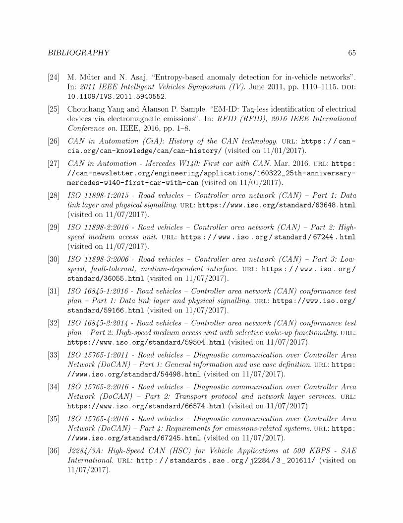
BIBLIOGRAPHY 65
[24] M. Muter and N. Asaj. “Entropy-based anomaly detection for in-vehicle networks”.In: 2011 IEEE Intelligent Vehicles Symposium (IV). June 2011, pp. 1110–1115. doi:10.1109/IVS.2011.5940552.
[25] Chouchang Yang and Alanson P. Sample. “EM-ID: Tag-less identification of electricaldevices via electromagnetic emissions”. In: RFID (RFID), 2016 IEEE InternationalConference on. IEEE, 2016, pp. 1–8.
[26] CAN in Automation (CiA): History of the CAN technology. url: https://can-
cia.org/can-knowledge/can/can-history/ (visited on 11/01/2017).
[27] CAN in Automation - Mercedes W140: First car with CAN. Mar. 2016. url: https://can-newsletter.org/engineering/applications/160322_25th-anniversary-
mercedes-w140-first-car-with-can (visited on 11/01/2017).
[28] ISO 11898-1:2015 - Road vehicles – Controller area network (CAN) – Part 1: Datalink layer and physical signalling. url: https://www.iso.org/standard/63648.html(visited on 11/07/2017).
[29] ISO 11898-2:2016 - Road vehicles – Controller area network (CAN) – Part 2: High-speed medium access unit. url: https://www.iso.org/standard/67244.html
(visited on 11/07/2017).
[30] ISO 11898-3:2006 - Road vehicles – Controller area network (CAN) – Part 3: Low-speed, fault-tolerant, medium-dependent interface. url: https : / / www . iso . org /
standard/36055.html (visited on 11/07/2017).
[31] ISO 16845-1:2016 - Road vehicles – Controller area network (CAN) conformance testplan – Part 1: Data link layer and physical signalling. url: https://www.iso.org/standard/59166.html (visited on 11/07/2017).
[32] ISO 16845-2:2014 - Road vehicles – Controller area network (CAN) conformance testplan – Part 2: High-speed medium access unit with selective wake-up functionality. url:https://www.iso.org/standard/59504.html (visited on 11/07/2017).
[33] ISO 15765-1:2011 - Road vehicles – Diagnostic communication over Controller AreaNetwork (DoCAN) – Part 1: General information and use case definition. url: https://www.iso.org/standard/54498.html (visited on 11/07/2017).
[34] ISO 15765-2:2016 - Road vehicles – Diagnostic communication over Controller AreaNetwork (DoCAN) – Part 2: Transport protocol and network layer services. url:https://www.iso.org/standard/66574.html (visited on 11/07/2017).
[35] ISO 15765-4:2016 - Road vehicles – Diagnostic communication over Controller AreaNetwork (DoCAN) – Part 4: Requirements for emissions-related systems. url: https://www.iso.org/standard/67245.html (visited on 11/07/2017).
[36] J2284/3A: High-Speed CAN (HSC) for Vehicle Applications at 500 KBPS - SAEInternational. url: http://standards.sae.org/j2284/3_201611/ (visited on11/07/2017).

BIBLIOGRAPHY 66
[37] Sae Mobilus. url: http : / / standards . sae . org / j2284 / 5 _ 201609/ (visited on11/07/2017).
[38] High-Speed CAN (HSC) for Vehicle Applications at 500 kbps with CAN FD Data at 2Mbps (J2284/4 Ground Vehicle Standard) - SAE Mobilus. url: http://standards.sae.org/j2284/4_201606/ (visited on 11/07/2017).
[39] High-Speed CAN (HSC) for Vehicle Applications at 500 KBPS (J2284/3 Ground Ve-hicle Standard) - SAE Mobilus. url: http://standards.sae.org/j2284/3_201611/(visited on 11/07/2017).
[40] High Speed CAN (HSC) for Vehicle Applications at 250 kbps (J2284/2 Ground VehicleStandard) - SAE Mobilus. url: http://standards.sae.org/j2284/2_201611/
(visited on 11/07/2017).
[41] High Speed CAN (HSC) for Vehicle Applications at 125 kbps (J2284/1 Ground VehicleStandard) - SAE Mobilus. url: http://standards.sae.org/j2284/1_201611/
(visited on 11/07/2017).
[42] J2411: Single Wire Can Network for Vehicle Applications - SAE International. url:http://standards.sae.org/j2411_200002/ (visited on 11/07/2017).
[43] Steve Corrigan. Introduction to the Controller Area Network. Aug. 2016. url: http://www.ti.com/lit/an/sloa101b/sloa101b.pdf (visited on 10/07/2017).
[44] Steve Corrigan. Controller Area Network Physical Layer Requirements. Jan. 2008. url:http://www.ti.com/lit/an/slla270/slla270.pdf (visited on 10/07/2017).
[45] Marco Di Natale. Understanding and using the Controller Area Network. Oct. 2008.url: http://inst.cs.berkeley.edu/~ee249/fa08/Lectures/handout_canbus2.pdf (visited on 10/24/2017).
[46] George Casella and Roger Berger. Statistical Inference. Second Edition. Duxbury Ad-vanced Series. Duxbury, 2002.
[47] Alper Demir and Alberto Sangiovanni-Vincentelli. Analysis and Simulation of Noise inNonlinear Electronic Circuits and Systems. DOI: 10.1007/978-1-4615-6063-0. Boston,MA: Springer US, 1998. isbn: 978-1-4613-7777-1 978-1-4615-6063-0. url: http://
link.springer.com/10.1007/978-1-4615-6063-0 (visited on 09/22/2017).
[48] Dmitry Panchenko. Kolmogorov-Smirnov Test. 2006. url: https://ocw.mit.edu/courses / mathematics / 18 - 443 - statistics - for - applications - fall - 2006 /
lecture-notes/lecture14.pdf.
[49] George Marsaglia, Wai Wan Tsang, and Jingbo Wang. “Evaluating Kolmogorov’s Dis-tribution”. In: Journal of Statistical Software 8.18 (2003), pp. 1–4. issn: 1548-7660.doi: 10.18637/jss.v008.i18. url: https://www.jstatsoft.org/article/view/v008i18 (visited on 09/23/2017).

BIBLIOGRAPHY 67
[50] Robert Gallager. Stochastic Processes: Theory for Applications. 1st ed. CambridgeUniversity Press, 2014. isbn: 978-1-107-03975-9. url: https://www.scribd.com/doc/152258575/Stochastic-Processes-Theory-for-Applications-by-Robert-
g-Gallager (visited on 10/02/2017).
[51] V. Kontorevich and V. Lyandres. “Impulsive noise: A nontraditional approach”. In:Signal Processing 51.2 (June 1996), pp. 121–132. issn: 0165-1684. doi: 10.1016/0165-1684(96)00036-9. url: http://www.sciencedirect.com/science/article/pii/0165168496000369 (visited on 09/30/2017).
[52] Gregory Kotler et al. “On the Markov model of shot noise”. In: Signal Processing(1999), pp. 79–88.
[53] P. Blanchard et al. “Stochastic dynamical aspects of neuronal activity”. en. In: Journalof Mathematical Biology 31.2 (Jan. 1993), pp. 189–198. issn: 0303-6812, 1432-1416.doi: 10.1007/BF00171226. url: https://link.springer.com/article/10.1007/BF00171226 (visited on 09/30/2017).
[54] A. Papoulis. “High Density Shot Noise and Gaussianity”. In: Journal of Applied Prob-ability 8.1 (1971), pp. 118–127. issn: 0021-9002. doi: 10.2307/3211842. url: http://www.jstor.org/stable/3211842 (visited on 09/30/2017).
[55] E. N. Gilbert and H. O. Pollak. “Amplitude distribution of shot noise”. In: The BellSystem Technical Journal 39.2 (Mar. 1960), pp. 333–350. issn: 0005-8580. doi: 10.1002/j.1538-7305.1960.tb01603.x.
[56] Rudolph Emil Kalman. “A new approach to linear filtering and prediction problems”.In: Journal of basic Engineering 82.1 (1960), pp. 35–45. url: https://fluidsengineering.asmedigitalcollection.asme.org/pdfaccess.ashx?resourceid=4506257&pdfsource=
13 (visited on 10/01/2017).
[57] Frederic Harris. “On the Use of Windows for Harmonic Analysis with the DiscreteFourier Transform”. In: Proceedings of the IEEE 66.1 (Jan. 1978), pp. 51–83.
[58] James W. Cooley and John W. Tukey. “An Algorithm for the Machine Calculation ofComplex Fourier Series”. In: Mathematics of Computation 19.90 (Apr. 1965), p. 297.issn: 00255718. doi: 10.2307/2003354. url: http://www.jstor.org/stable/
2003354?origin=crossref (visited on 09/20/2017).
[59] P. Welch. “The use of fast Fourier transform for the estimation of power spectra:A method based on time averaging over short, modified periodograms”. In: IEEETransactions on Audio and Electroacoustics 15.2 (June 1967), pp. 70–73. issn: 0018-9278. doi: 10.1109/TAU.1967.1161901.
[60] Hirotugu Akaike. “Fitting autoregressive models for prediction”. In: Annals of theinstitute of Statistical Mathematics 21.1 (1969), pp. 243–247.
[61] Hirotugu Akaike. “Power spectrum estimation through autoregressive model fitting”.In: Annals of the Institute of Statistical Mathematics 21.1 (Dec. 1969), pp. 407–419.

BIBLIOGRAPHY 68
[62] I. Daubechies. “Where do wavelets come from? A personal point of view”. In: Proceed-ings of the IEEE 84.4 (Apr. 1996), pp. 510–513. issn: 0018-9219. doi: 10.1109/5.488696.
[63] Fabian Morchen. Time series feature extraction for data mining using DWT and DFT.Tech. rep. 2003.
[64] A. Graps. “An introduction to wavelets”. In: IEEE Computational Science and Engi-neering 2.2 (1995), pp. 50–61. issn: 1070-9924. doi: 10.1109/99.388960.
[65] Ingrid Daubechies. “Orthonormal bases of compactly supported wavelets”. In: Com-munications on pure and applied mathematics 41.7 (1988), pp. 909–996. url: http://onlinelibrary.wiley.com/doi/10.1002/cpa.3160410705/full (visited on09/27/2017).
[66] Ben D. Fulcher, Max A. Little, and Nick S. Jones. “Highly comparative time-seriesanalysis: the empirical structure of time series and their methods”. en. In: Journalof The Royal Society Interface 10.83 (June 2013), p. 20130048. issn: 1742-5689, 1742-5662. doi: 10.1098/rsif.2013.0048. url: http://rsif.royalsocietypublishing.org/content/10/83/20130048 (visited on 10/08/2017).
[67] B. D. Fulcher and N. S. Jones. “Highly Comparative Feature-Based Time-Series Clas-sification”. In: IEEE Transactions on Knowledge and Data Engineering 26.12 (Dec.2014), pp. 3026–3037. issn: 1041-4347. doi: 10.1109/TKDE.2014.2316504.
[68] Thomas Schreiber and Andreas Schmitz. “Surrogate time series”. In: Physica D: Non-linear Phenomena 142.3 (Aug. 2000), pp. 346–382. issn: 0167-2789. doi: 10.1016/S0167 - 2789(00 ) 00043 - 9. url: http : / / www . sciencedirect . com / science /
article/pii/S0167278900000439 (visited on 10/08/2017).
[69] D. N. Joanes and C. A. Gill. “Comparing Measures of Sample Skewness and Kurtosis”.In: Journal of the Royal Statistical Society. Series D (The Statistician) 47.1 (1998),pp. 183–189. issn: 0039-0526. url: http://www.jstor.org/stable/2988433 (visitedon 10/08/2017).
[70] Andrew Ng. Machine Learning. Lecture. Coursera.com, 2017. url: https://www.
coursera.org/learn/machine-learning?authMode=login (visited on 10/01/2017).
[71] G. P. Zhang. “Neural networks for classification: a survey”. In: IEEE Transactions onSystems, Man, and Cybernetics, Part C (Applications and Reviews) 30.4 (Nov. 2000),pp. 451–462. issn: 1094-6977. doi: 10.1109/5326.897072.
[72] Anders Krogh and John A. Hertz. “A Simple Weight Decay Can Improve Generaliza-tion”. In: Advances in Neural Information Processing Systems 4. Morgan Kaufmann,1992, pp. 950–957.
[73] Andreas Weigend, Bernardo Huberman, and David Rumelhart. “Generalization byWeight-Elimination with Application to Forecasting”. In: Int. J. Neural Syst. 1 (Jan.1990), pp. 193–209. doi: 10.1142/S0129065790000102.

BIBLIOGRAPHY 69
[74] Nitish Srivastava et al. “Dropout: A Simple Way to Prevent Neural Networks fromOverfitting”. In: Journal of Machine Learning Research 15 (June 2014), pp. 1929–1958. url: http://jmlr.csail.mit.edu/papers/v15/srivastava14a.html (visitedon 10/01/2017).
[75] Jonathan Richard Shewchuk et al. An introduction to the conjugate gradient methodwithout the agonizing pain. Carnegie-Mellon University. Department of Computer Sci-ence, 1994. url: ftp://ftp.unicauca.edu.co/Facultades/.FIET_serepiteencuentasyocupaespacio/DEIC/docs/Materias/computacion%20inteligente/parte%20II/semana12/gradient/
painless-conjugate-gradient.pdf (visited on 10/02/2017).
[76] Chih-Jen Lin. “Probability estimates for multi-class classification by pairwise cou-pling”. In: The Journal of Machine Learning Research (Aug. 2004). url: http://www.academia.edu/2834474/Probability_estimates_for_multi-class_classification_
by_pairwise_coupling (visited on 09/29/2017).
[77] Johan AK Suykens and Joos Vandewalle. “Least squares support vector machine clas-sifiers”. In: Neural processing letters 9.3 (1999), pp. 293–300. url: http: //www.
springerlink.com/index/n75178640w32646j.pdf (visited on 09/29/2017).
[78] Jason Weston. Support Vector Machine Tutuorial. url: http://www.cs.columbia.edu/~kathy/cs4701/documents/jason_svm_tutorial.pdf (visited on 09/30/2017).
[79] Kurt Hornik. “Approximation capabilities of multilayer feedforward networks”. In:Neural Networks 4.2 (Jan. 1991), pp. 251–257. issn: 0893-6080. doi: 10.1016/0893-6080(91)90009-T. url: http://www.sciencedirect.com/science/article/pii/089360809190009T (visited on 09/27/2017).
[80] “Learning Polynomials with Neural Networks”. eng. In: Proceedings of the 31 st In-ternational Conference on Machine Learning. Ed. by Alexandr Andoni et al. Vol. 32.OCLC: 179807959. Beijing, China: ACM Press, 2014. isbn: 978-1-58113-960-0.
[81] M. Bianchini and F. Scarselli. “On the Complexity of Neural Network Classifiers: AComparison Between Shallow and Deep Architectures”. In: IEEE Transactions onNeural Networks and Learning Systems 25.8 (Aug. 2014), pp. 1553–1565. issn: 2162-237X. doi: 10.1109/TNNLS.2013.2293637.
[82] D. Hunter et al. “Selection of Proper Neural Network Sizes and Architectures: A Com-parative Study”. In: IEEE Transactions on Industrial Informatics 8.2 (May 2012),pp. 228–240. issn: 1551-3203. doi: 10.1109/TII.2012.2187914.
[83] Chistopher Bishop. Pattern Recognition and Machine Learning. Springer US, 2006.
[84] Avrim L. Blum and Pat Langley. “Selection of relevant features and examples inmachine learning”. In: Artificial Intelligence. Relevance 97.1 (Dec. 1997), pp. 245–271. issn: 0004-3702. doi: 10 . 1016 / S0004 - 3702(97 ) 00063 - 5. url: http : / /
www.sciencedirect.com/science/article/pii/S0004370297000635 (visited on09/28/2017).
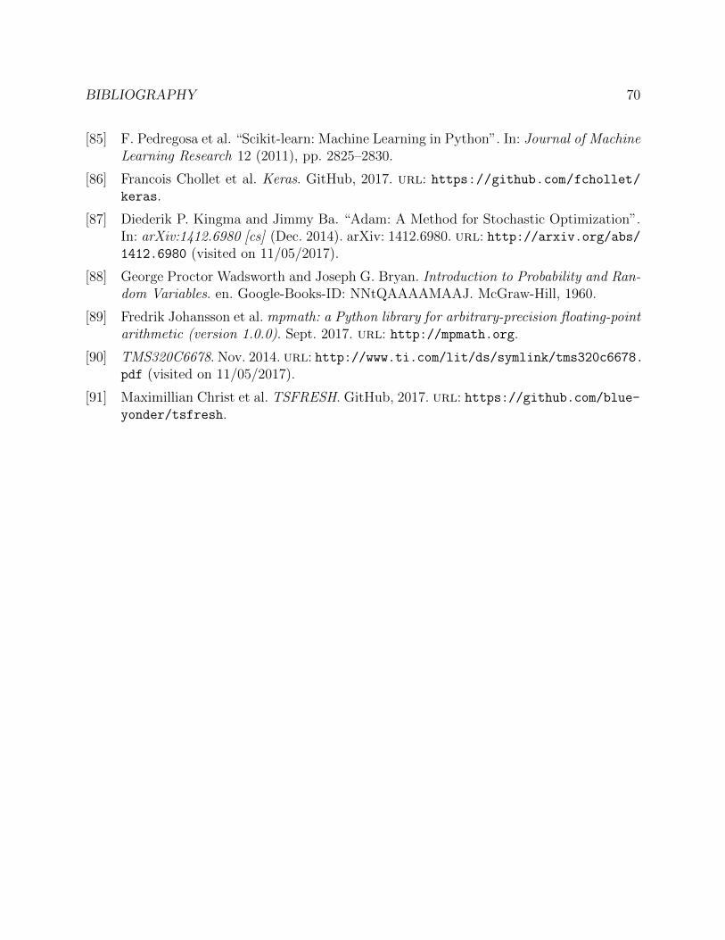
BIBLIOGRAPHY 70
[85] F. Pedregosa et al. “Scikit-learn: Machine Learning in Python”. In: Journal of MachineLearning Research 12 (2011), pp. 2825–2830.
[86] Francois Chollet et al. Keras. GitHub, 2017. url: https://github.com/fchollet/keras.
[87] Diederik P. Kingma and Jimmy Ba. “Adam: A Method for Stochastic Optimization”.In: arXiv:1412.6980 [cs] (Dec. 2014). arXiv: 1412.6980. url: http://arxiv.org/abs/1412.6980 (visited on 11/05/2017).
[88] George Proctor Wadsworth and Joseph G. Bryan. Introduction to Probability and Ran-dom Variables. en. Google-Books-ID: NNtQAAAAMAAJ. McGraw-Hill, 1960.
[89] Fredrik Johansson et al. mpmath: a Python library for arbitrary-precision floating-pointarithmetic (version 1.0.0). Sept. 2017. url: http://mpmath.org.
[90] TMS320C6678. Nov. 2014. url: http://www.ti.com/lit/ds/symlink/tms320c6678.pdf (visited on 11/05/2017).
[91] Maximillian Christ et al. TSFRESH. GitHub, 2017. url: https://github.com/blue-yonder/tsfresh.
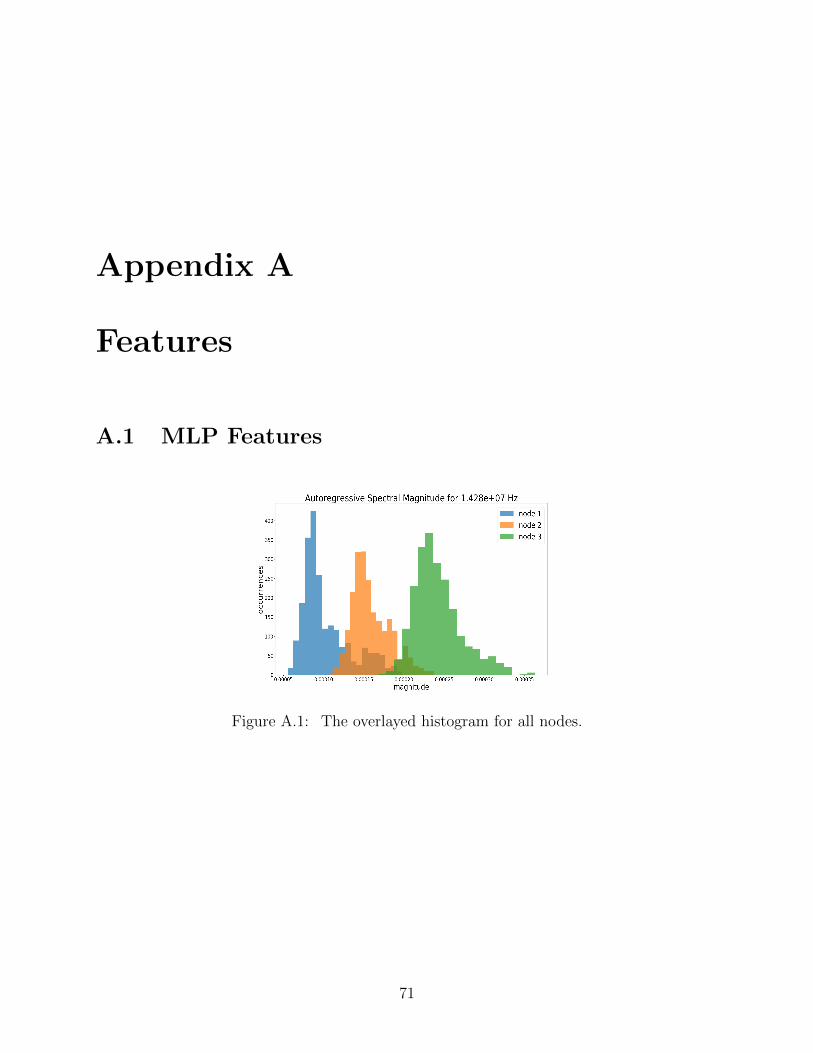
Appendix A
Features
A.1 MLP Features
Figure A.1: The overlayed histogram for all nodes.
71
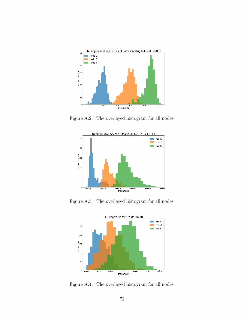
Figure A.2: The overlayed histogram for all nodes.
Figure A.3: The overlayed histogram for all nodes.
Figure A.4: The overlayed histogram for all nodes.
72

Figure A.5: The overlayed histogram for all nodes.
Figure A.6: The overlayed histogram for all nodes.
Figure A.7: The overlayed histogram for all nodes.
73

Figure A.8: The overlayed histogram for all nodes.
Figure A.9: The overlayed histogram for all nodes.
Figure A.10: The overlayed histogram for all nodes.
74
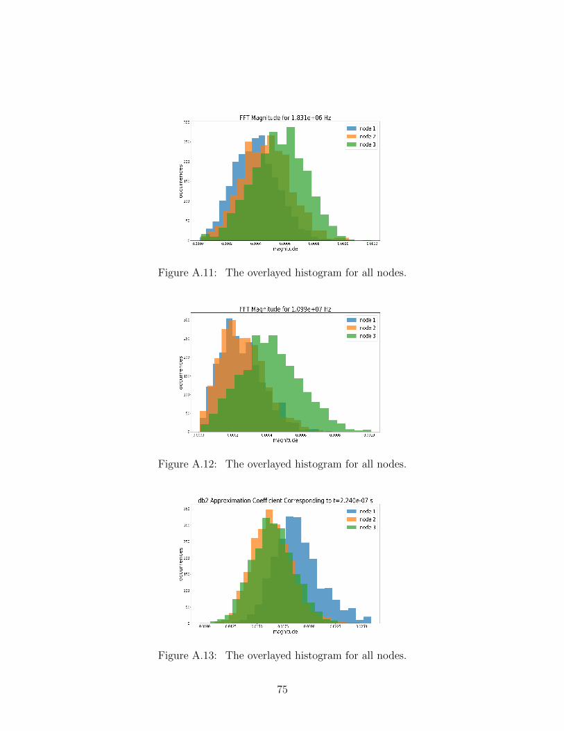
Figure A.11: The overlayed histogram for all nodes.
Figure A.12: The overlayed histogram for all nodes.
Figure A.13: The overlayed histogram for all nodes.
75

Figure A.14: The overlayed histogram for all nodes.
Figure A.15: The overlayed histogram for all nodes.
Figure A.16: The overlayed histogram for all nodes.
76
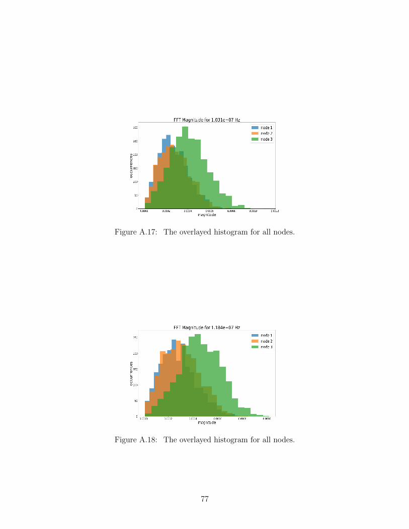
Figure A.17: The overlayed histogram for all nodes.
Figure A.18: The overlayed histogram for all nodes.
77

BIBLIOGRAPHY 78
A.2 SVM Features
Figure A.19: The overlayed histogram for all nodes.
Figure A.20: The overlayed histogram for all nodes.

BIBLIOGRAPHY 79
Figure A.21: The overlayed histogram for all nodes.
Figure A.22: The overlayed histogram for all nodes.
Figure A.23: The overlayed histogram for all nodes.
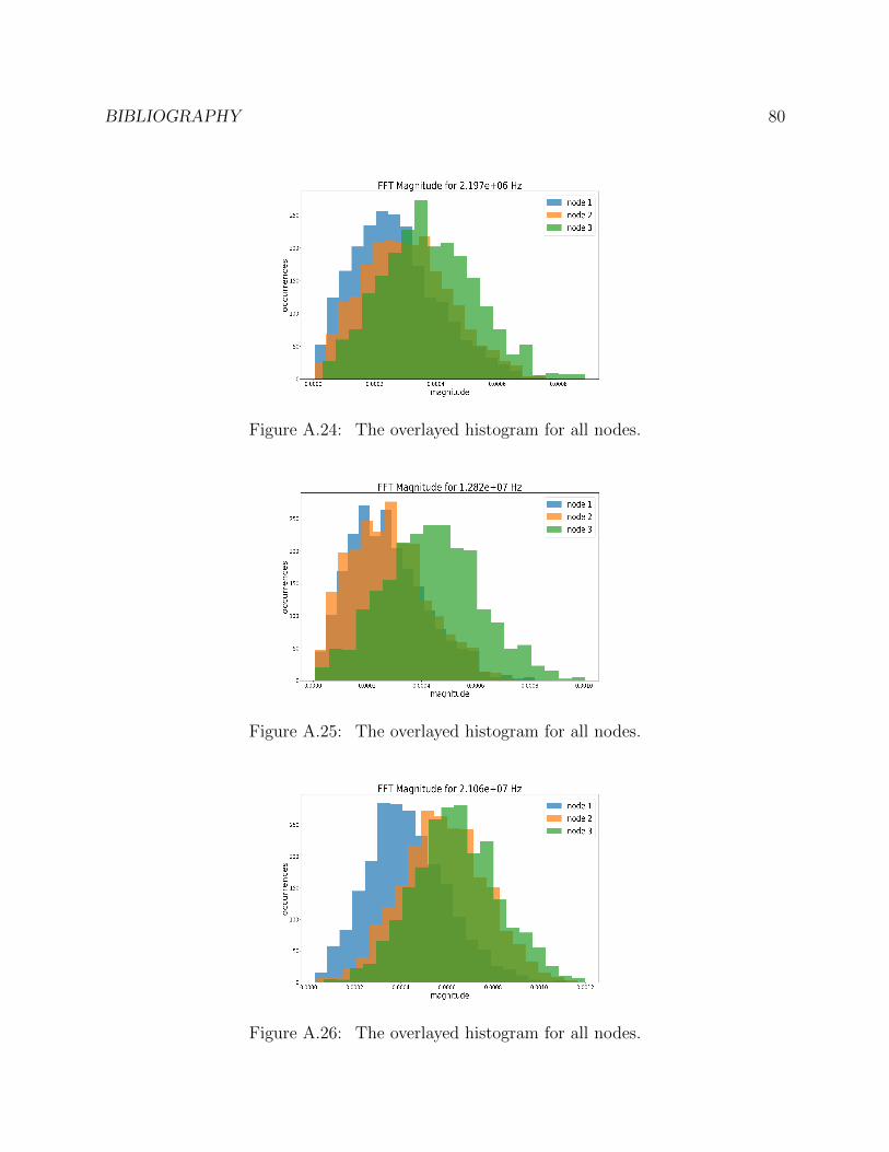
BIBLIOGRAPHY 80
Figure A.24: The overlayed histogram for all nodes.
Figure A.25: The overlayed histogram for all nodes.
Figure A.26: The overlayed histogram for all nodes.