introductory econometrics – kunst – university of...
TRANSCRIPT
Introduction Repetition of statistical terminology Simple linear regression model
Introductory EconometricsBased on the textbook by Ramanathan:
Introductory Econometrics
Robert M. [email protected]
University of Viennaand
Institute for Advanced Studies Vienna
September 23, 2011
Introductory Econometrics University of Vienna and Institute for Advanced Studies Vienna
Introduction Repetition of statistical terminology Simple linear regression model
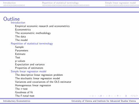
OutlineIntroduction
Empirical economic research and econometricsEconometricsThe econometric methodologyThe dataThe model
Repetition of statistical terminologySampleParametersEstimateTestp–valuesExpectation and varianceProperties of estimators
Simple linear regression modelThe descriptive linear regression problemThe stochastic linear regression modelVariances and covariances of the OLS estimatorHomogeneous linear regressionThe t–testGoodness of fitThe F-total–test
Introductory Econometrics University of Vienna and Institute for Advanced Studies Vienna
Introduction Repetition of statistical terminology Simple linear regression model
Empirical economic research and econometrics
Empirical economic research and econometrics
Empirical economic research is the internal wording forintroductory econometrics. Econometrics focuses on the interfaceof economic theory and the actual economic world.
The information on economics comes in the shape of data.
This data (quantitative rather than qualitative) is the subject ofthe analysis.
In current usage, methods for the statistical analysis of the dataare called ‘econometrics’, not for the gathering or compilation ofthe data.
Introductory Econometrics University of Vienna and Institute for Advanced Studies Vienna
Introduction Repetition of statistical terminology Simple linear regression model
Econometrics
Econometrics
Word appears for the first time around 1900: analogy constructionto biometrics etc.
Founding of the Econometric Society and its journal Econometrica
(1930, Ragnar Frisch and others): mathematical and statistical
methods in economics.
Today, mathematical methods in economics (mathematicaleconomics) are no more regarded as ‘econometrics’, while theycontinue to dominate the Econometric Society and alsoEconometrica.
Introductory Econometrics University of Vienna and Institute for Advanced Studies Vienna
Introduction Repetition of statistical terminology Simple linear regression model
Econometrics
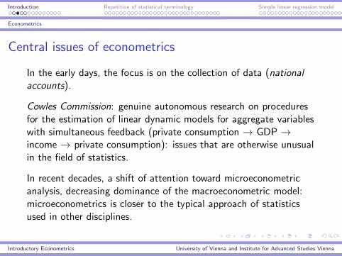
Central issues of econometrics
In the early days, the focus is on the collection of data (nationalaccounts).
Cowles Commission: genuine autonomous research on proceduresfor the estimation of linear dynamic models for aggregate variableswith simultaneous feedback (private consumption → GDP →income → private consumption): issues that are otherwise unusualin the field of statistics.
In recent decades, a shift of attention toward microeconometricanalysis, decreasing dominance of the macroeconometric model:microeconometrics is closer to the typical approach of statisticsused in other disciplines.
Introductory Econometrics University of Vienna and Institute for Advanced Studies Vienna
Introduction Repetition of statistical terminology Simple linear regression model
Econometrics
Selected textbooks of econometrics
◮ Ramanathan, R. (2002). Introductory Econometrics with
Applications. 5th edition, South-Western.
◮ Berndt, E.R. (1991). The Practice of Econometrics.Addison-Wesley.
◮ Greene, W.H. (2008). Econometric Analysis. 6th edition,Prentice-Hall.
◮ Hayashi, F. (2000). Econometrics. Princeton.
◮ Johnston, J. and DiNardo, J. (1997). Econometric
Methods. 4th edition, McGraw-Hill.
◮ Stock, J.H., and Watson, M.W. (2007). Introduction to
Econometrics. Addison-Wesley.
◮ Wooldridge, J.M. (2009). Introductory Econometrics. 4thedition, South-Western.
Introductory Econometrics University of Vienna and Institute for Advanced Studies Vienna
Introduction Repetition of statistical terminology Simple linear regression model
Econometrics
Aims of econometric analysis
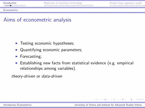
◮ Testing economic hypotheses;
◮ Quantifying economic parameters;
◮ Forecasting;
◮ Establishing new facts from statistical evidence (e.g. empiricalrelationships among variables).
theory-driven or data-driven
Introductory Econometrics University of Vienna and Institute for Advanced Studies Vienna
Introduction Repetition of statistical terminology Simple linear regression model
The econometric methodology
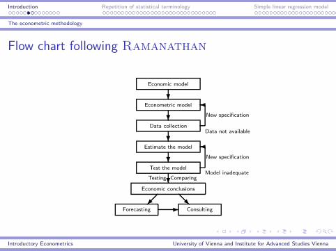
Flow chart following Ramanathan
Economic model
?Econometric model
?Data collection
Data not available
New specification
�
?Estimate the model
?Test the model
Model inadequate
New specification
�
?Testing Comparing
Economic conclusions
Forecasting Consulting
�� @@R-
Introductory Econometrics University of Vienna and Institute for Advanced Studies Vienna
Introduction Repetition of statistical terminology Simple linear regression model
The econometric methodology
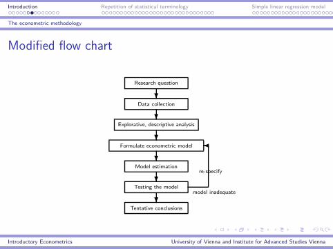
Modified flow chart
Research question
?Data collection
?Explorative, descriptive analysis
?Formulate econometric model
?Model estimation
?Testing the model
model inadequate
re-specify
�
?Tentative conclusions
Introductory Econometrics University of Vienna and Institute for Advanced Studies Vienna
Introduction Repetition of statistical terminology Simple linear regression model
The data
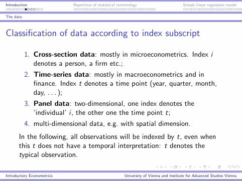
Classification of data according to index subscript
1. Cross-section data: mostly in microeconometrics. Index i
denotes a person, a firm etc.;
2. Time-series data: mostly in macroeconometrics and infinance. Index t denotes a time point (year, quarter, month,day, . . . );
3. Panel data: two-dimensional, one index denotes the‘individual’ i , the other one the time point t;
4. multi-dimensional data, e.g. with spatial dimension.
In the following, all observations will be indexed by t, even whenthis t does not have a temporal interpretation: t denotes thetypical observation.
Introductory Econometrics University of Vienna and Institute for Advanced Studies Vienna
Introduction Repetition of statistical terminology Simple linear regression model
The data
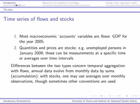
Time series of flows and stocks
1. Most macroeconomic ‘accounts’ variables are flows: GDP forthe year 2005;
2. Quantities and prices are stocks: e.g. unemployed persons inJanuary 2009; these can be measurements at a specific timeor averages over time intervals.
Differences between the two types concern temporal aggregation:with flows, annual data evolve from monthly data by sums(accumulation); with stocks, one may use averages over monthlyobservations, though sometimes other conventions are used.
Introductory Econometrics University of Vienna and Institute for Advanced Studies Vienna
Introduction Repetition of statistical terminology Simple linear regression model
The data
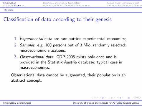
Classification of data according to their genesis
1. Experimental data are rare outside experimental economics;
2. Samples: e.g. 100 persons out of 3 Mio. randomly selected:microeconomic situations;
3. Observational data: GDP 2005 exists only once and isprovided in the Statistik Austria database: typical case inmacroeconomics.
Observational data cannot be augmented, their population is anabstract concept.
Introductory Econometrics University of Vienna and Institute for Advanced Studies Vienna
Introduction Repetition of statistical terminology Simple linear regression model
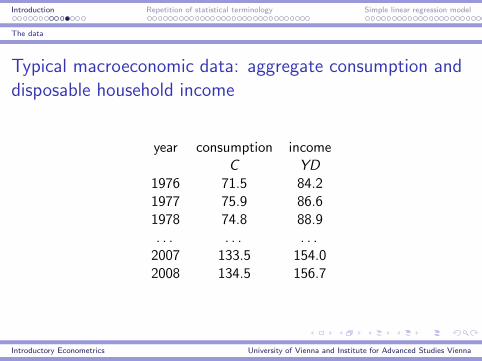
The data
Typical macroeconomic data: aggregate consumption and
disposable household income
year consumption incomeC YD
1976 71.5 84.21977 75.9 86.61978 74.8 88.9. . . . . . . . .2007 133.5 154.02008 134.5 156.7
Introductory Econometrics University of Vienna and Institute for Advanced Studies Vienna
Introduction Repetition of statistical terminology Simple linear regression model
The model
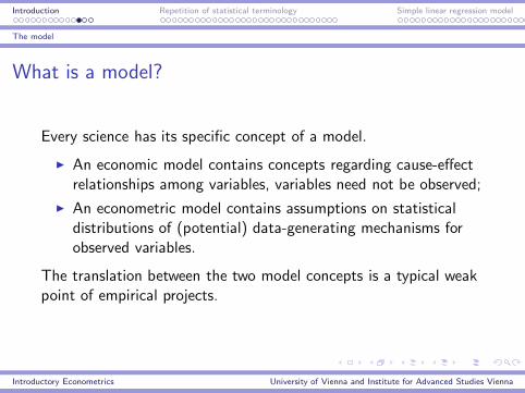
What is a model?
Every science has its specific concept of a model.
◮ An economic model contains concepts regarding cause-effectrelationships among variables, variables need not be observed;
◮ An econometric model contains assumptions on statisticaldistributions of (potential) data-generating mechanisms forobserved variables.
The translation between the two model concepts is a typical weakpoint of empirical projects.
Introductory Econometrics University of Vienna and Institute for Advanced Studies Vienna
Introduction Repetition of statistical terminology Simple linear regression model
The model
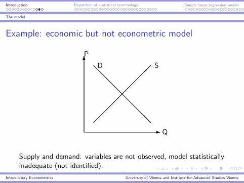
Example: economic but not econometric model
6
-�
��������@
@@@@@@@@
Q
P
D S
Supply and demand: variables are not observed, model statisticallyinadequate (not identified).
Introductory Econometrics University of Vienna and Institute for Advanced Studies Vienna
Introduction Repetition of statistical terminology Simple linear regression model
The model
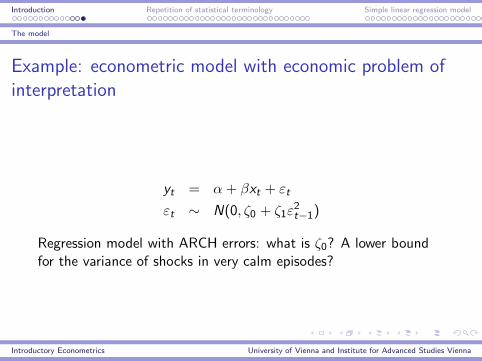
Example: econometric model with economic problem of
interpretation
yt = α+ βxt + εt
εt ∼ N(0, ζ0 + ζ1ε2t−1)
Regression model with ARCH errors: what is ζ0? A lower boundfor the variance of shocks in very calm episodes?
Introductory Econometrics University of Vienna and Institute for Advanced Studies Vienna
Introduction Repetition of statistical terminology Simple linear regression model
Sample
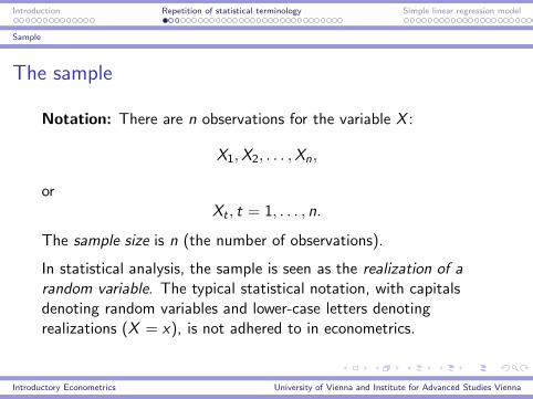
The sample
Notation: There are n observations for the variable X :
X1,X2, . . . ,Xn,
orXt , t = 1, . . . , n.
The sample size is n (the number of observations).
In statistical analysis, the sample is seen as the realization of a
random variable. The typical statistical notation, with capitalsdenoting random variables and lower-case letters denotingrealizations (X = x), is not adhered to in econometrics.
Introductory Econometrics University of Vienna and Institute for Advanced Studies Vienna
Introduction Repetition of statistical terminology Simple linear regression model
Sample
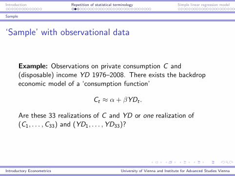
‘Sample’ with observational data
Example: Observations on private consumption C and(disposable) income YD 1976–2008. There exists the backdropeconomic model of a ‘consumption function’
Ct ≈ α+ βYDt .
Are these 33 realizations of C and YD or one realization of(C1, . . . ,C33) and (YD1, . . . ,YD33)?
Introductory Econometrics University of Vienna and Institute for Advanced Studies Vienna
Introduction Repetition of statistical terminology Simple linear regression model
Sample
Usefulness or honesty?
◮ 33 realizations of one random variable: C and YD areincreasing over time, time dependence (business cycle, inertiain the reaction of households), changes in economic behavior:implausible. Parameters of the consumption function can beestimated with reasonable precision.
◮ One realization: Interpretation of unobserved realizationsbecomes problematic (parallel universes?). Parameters of theconsumption function cannot be estimated from oneobservation.
Way out: not the variables, but the unobserved error term is therandom variable: 33 observations, ‘shocks stationary’, consumptionfunction again estimable.
Introductory Econometrics University of Vienna and Institute for Advanced Studies Vienna
Introduction Repetition of statistical terminology Simple linear regression model
Parameters
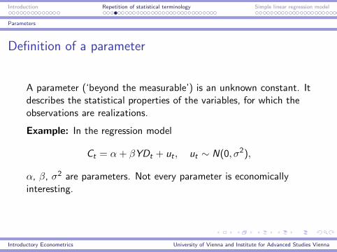
Definition of a parameter
A parameter (‘beyond the measurable’) is an unknown constant. Itdescribes the statistical properties of the variables, for which theobservations are realizations.
Example: In the regression model
Ct = α+ βYDt + ut , ut ∼ N(0, σ2),
α, β, σ2 are parameters. Not every parameter is economicallyinteresting.
Introductory Econometrics University of Vienna and Institute for Advanced Studies Vienna
Introduction Repetition of statistical terminology Simple linear regression model
Estimate
Definition of an estimator
An estimator is a specific function of the data that is designed toapproximate a parameter. Its realization for given data is calledestimate.
The word ‘estimator’ is used for the random variable that evolvesfrom calculating the function of a virtual sample—a statistic—andfor the functional form proper. Statistics calculated from observeddata are observed. If data are assumed to be realizations ofrandom variables, all statistics calculated from them and also theestimators are random variables, while estimates are realizations ofthese random variables. Parameters are unobserved.
Introductory Econometrics University of Vienna and Institute for Advanced Studies Vienna
Introduction Repetition of statistical terminology Simple linear regression model
Estimate
Notation for estimates and parameters
Parameters are usually denoted by Greek letters: α,β,θ,. . .
The corresponding estimates or estimators are denoted by a hat:α, β, θ, . . . Latin letters (a estimates α etc.) are also used by someauthors.
Introductory Econometrics University of Vienna and Institute for Advanced Studies Vienna
Introduction Repetition of statistical terminology Simple linear regression model
Estimate
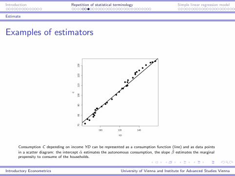
Examples of estimators
100 120 140
7080
9010
011
012
013
0
YD
C
Consumption C depending on income YD can be represented as a consumption function (line) and as data points
in a scatter diagram: the intercept α estimates the autonomous consumption, the slope β estimates the marginalpropensity to consume of the households.
Introductory Econometrics University of Vienna and Institute for Advanced Studies Vienna
Introduction Repetition of statistical terminology Simple linear regression model
Test
Definition of the hypothesis test
A test is a statistical decision rule. The aim is a decision whetherthe data suggest that a specified hypothesis is incorrect (‘toreject’) or correct (‘not to reject’, ‘to accept’, ‘fail to reject’).
It is customary first to calculate a test statistic from the data, areal number that is a function of the data. If this statistic is in therejection region (critical region), the test is said to reject.
Introductory Econometrics University of Vienna and Institute for Advanced Studies Vienna
Introduction Repetition of statistical terminology Simple linear regression model
Test
Tests: common mistakes
◮ A test is not a test statistic. The test statistic is a realnumber, whereas the test itself can only indicate rejection oracceptance (‘non-rejection’), a decision that may be coded by0/1. A test cannot be 1.5.
◮ A test is not a null hypothesis. A test cannot be rejected.The tested hypothesis can be rejected. The test rejects.
Introductory Econometrics University of Vienna and Institute for Advanced Studies Vienna
Introduction Repetition of statistical terminology Simple linear regression model
Test
Do economic theories deserve a presumption of innocence?
The null hypothesis (or short null) is a (typically sharp) statementon a parameter. Example: β = 1. These statements oftencorrespond to an economic theory.
The alternative hypothesis (or short alternative) is often thenegation of the null within the framework of a general hypothesis(maintained hypothesis). Example: β ∈ (0, 1) ∪ (1,∞). Thisstatement often corresponds to the invalidity of an economictheory.
Notation: H0 for the null hypothesis and e.g. HA for thealternative. H0 ∪ HA is the general or maintained hypothesis.Example: the maintained hypothesis β > 0 is not tested butassumed (‘window on the world’).
Introductory Econometrics University of Vienna and Institute for Advanced Studies Vienna
Introduction Repetition of statistical terminology Simple linear regression model
Test
Hypotheses: common mistakes
◮ A hypothesis cannot be a statement on an estimate.“H0 : β = 0” is meaningless, as β can be determined exactlyfrom data.
◮ Alternatives cannot be rejected. The classical hypothesestest is asymmetrical. Only H0 can be rejected or ‘accepted’.(Bayes tests are non-classical and follow different rules)
◮ Hypotheses do not have probabilities. H0 is never correctwith a probability of 90% after testing. (Bayes tests allotprobabilities to hypotheses)
Introductory Econometrics University of Vienna and Institute for Advanced Studies Vienna
Introduction Repetition of statistical terminology Simple linear regression model
Test
Errors of type I and of type II
The parameters are unobserved and can only be determinedapproximately from the sample. For this reason, decisions are oftenincorrect:
◮ If the test rejects, although the null hypothesis is correct, thisis a type I error;
◮ If the test accepts the null, although it is incorrect, this is atype II error.
A basic construction principle of classical hypothesis tests is toprescribe a bound on the probability of type I errors (e.g. by 1%,5%) and, given this bound, to minimize the probability of a type IIerror.
Introductory Econometrics University of Vienna and Institute for Advanced Studies Vienna
Introduction Repetition of statistical terminology Simple linear regression model
Test
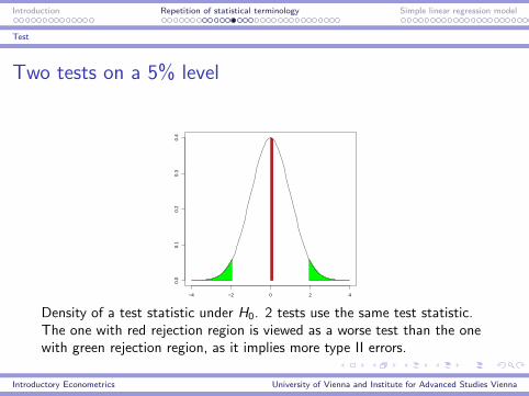
Two tests on a 5% level
−4 −2 0 2 4
0.0
0.1
0.2
0.3
0.4
Density of a test statistic under H0. 2 tests use the same test statistic.The one with red rejection region is viewed as a worse test than the onewith green rejection region, as it implies more type II errors.
Introductory Econometrics University of Vienna and Institute for Advanced Studies Vienna
Introduction Repetition of statistical terminology Simple linear regression model
Test
More vocabulary on tests
The often pre-specified probability of a type I error is called thesize of the test or the significance level. For simple nullhypotheses, it will be approximately constant under H0, otherwiseit is an upper bound.
The probability not to make a type II error is called the power ofthe test. It is defined on the alternative, and it depends on the‘distance’ from H0. Close to H0, power will be low (close to size);at locations far from H0, it approaches 1.
If the test attains a power of 1 on the entire alternative, as thesample size grows toward ∞, the test will be called consistent.
Introductory Econometrics University of Vienna and Institute for Advanced Studies Vienna
Introduction Repetition of statistical terminology Simple linear regression model
Test
Best tests
A concept analogous to efficient estimators, a test that attainsmaximal power at given size, exists for some simple problems only.For most test problems, however, the likelihood-ratio test (LR test,the test statistic is a ratio of the maxima of the likelihood underH0 and HA) has good power properties.
Often, the Wald test and the LM test (Lagrange multiplier)represent ‘cheaper’ approximations to LR and still they haveidentical properties for large n .
Attention: LR, LM and Wald test are construction principles fortests, not specific tests. It does not make sense to say that ‘theWald test rejects’, unless it is also indicated what is being tested.
Introductory Econometrics University of Vienna and Institute for Advanced Studies Vienna
Introduction Repetition of statistical terminology Simple linear regression model
Test
Can a presumption of innocence apply to the invalidity of a
theory?
Economic statements need not correspond to the null of ahypothesis test. Sometimes, the null hypothesis is the invalidity ofa theory. For example, theory may tell that the export ratiodepends on the exchange rate.
Even then, the null of the test corresponds to the more restrictivestatement. The economic statement becomes the alternative. Theinvalidity of the economic theory can be rejected. For example, H0
says that the coefficient of the export ratio that depends on theexchange rate is 0, and this is rejected.
Introductory Econometrics University of Vienna and Institute for Advanced Studies Vienna
Introduction Repetition of statistical terminology Simple linear regression model
p–values
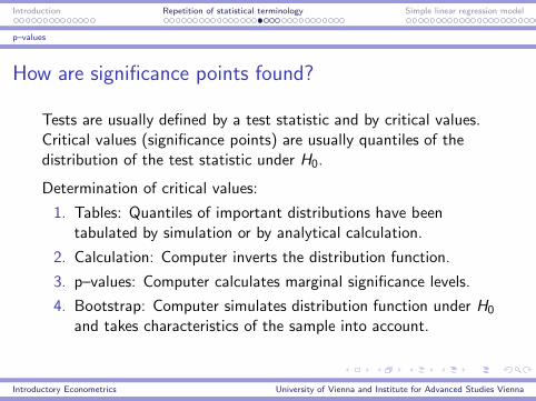
How are significance points found?
Tests are usually defined by a test statistic and by critical values.Critical values (significance points) are usually quantiles of thedistribution of the test statistic under H0.
Determination of critical values:
1. Tables: Quantiles of important distributions have beentabulated by simulation or by analytical calculation.
2. Calculation: Computer inverts the distribution function.
3. p–values: Computer calculates marginal significance levels.
4. Bootstrap: Computer simulates distribution function under H0
and takes characteristics of the sample into account.
Introductory Econometrics University of Vienna and Institute for Advanced Studies Vienna
Introduction Repetition of statistical terminology Simple linear regression model
p–values
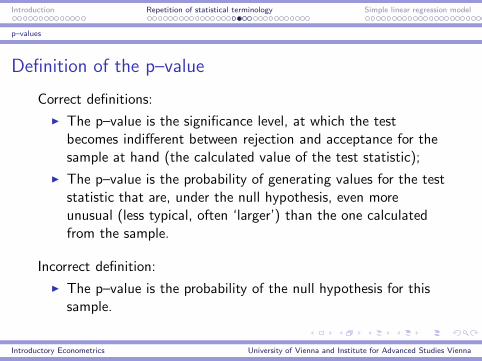
Definition of the p–value
Correct definitions:
◮ The p–value is the significance level, at which the testbecomes indifferent between rejection and acceptance for thesample at hand (the calculated value of the test statistic);
◮ The p–value is the probability of generating values for the teststatistic that are, under the null hypothesis, even moreunusual (less typical, often ‘larger’) than the one calculatedfrom the sample.
Incorrect definition:
◮ The p–value is the probability of the null hypothesis for thissample.
Introductory Econometrics University of Vienna and Institute for Advanced Studies Vienna
Introduction Repetition of statistical terminology Simple linear regression model
p–values
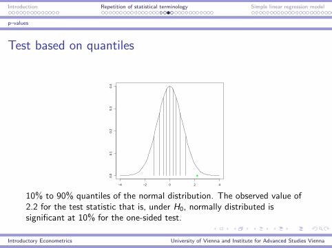
Test based on quantiles
−4 −2 0 2 4
0.0
0.1
0.2
0.3
0.4
10% to 90% quantiles of the normal distribution. The observed value of2.2 for the test statistic that is, under H0, normally distributed issignificant at 10% for the one-sided test.
Introductory Econometrics University of Vienna and Institute for Advanced Studies Vienna
Introduction Repetition of statistical terminology Simple linear regression model
p–values
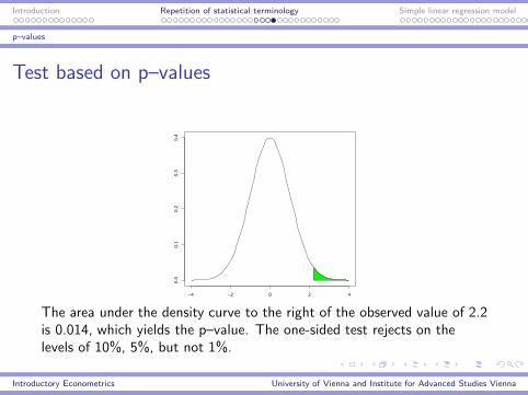
Test based on p–values
−4 −2 0 2 4
0.0
0.1
0.2
0.3
0.4
The area under the density curve to the right of the observed value of 2.2is 0.014, which yields the p–value. The one-sided test rejects on thelevels of 10%, 5%, but not 1%.
Introductory Econometrics University of Vienna and Institute for Advanced Studies Vienna
Introduction Repetition of statistical terminology Simple linear regression model
Expectation and variance
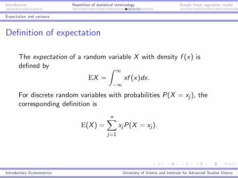
Definition of expectation
The expectation of a random variable X with density f (x) isdefined by
EX =
∫∞
−∞
xf (x)dx .
For discrete random variables with probabilities P(X = xj), thecorresponding definition is
E(X ) =n∑
j=1
xjP(X = xj).
Introductory Econometrics University of Vienna and Institute for Advanced Studies Vienna
Introduction Repetition of statistical terminology Simple linear regression model
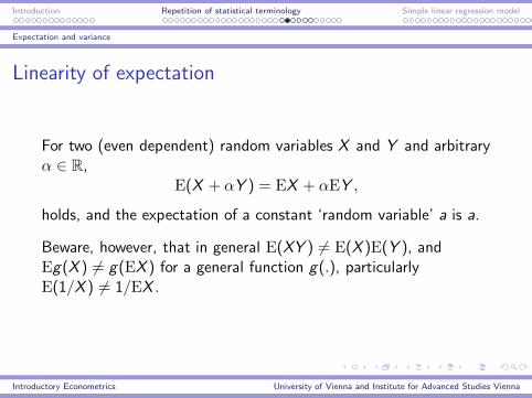
Expectation and variance
Linearity of expectation
For two (even dependent) random variables X and Y and arbitraryα ∈ R,
E(X + αY ) = EX + αEY ,
holds, and the expectation of a constant ‘random variable’ a is a.
Beware, however, that in general E(XY ) 6= E(X )E(Y ), andEg(X ) 6= g(EX ) for a general function g(.), particularlyE(1/X ) 6= 1/EX .
Introductory Econometrics University of Vienna and Institute for Advanced Studies Vienna
Introduction Repetition of statistical terminology Simple linear regression model
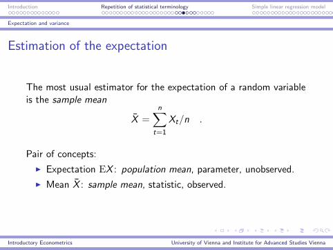
Expectation and variance
Estimation of the expectation
The most usual estimator for the expectation of a random variableis the sample mean
X =n∑
t=1
Xt/n .
Pair of concepts:
◮ Expectation EX : population mean, parameter, unobserved.
◮ Mean X : sample mean, statistic, observed.
Introductory Econometrics University of Vienna and Institute for Advanced Studies Vienna
Introduction Repetition of statistical terminology Simple linear regression model
Expectation and variance
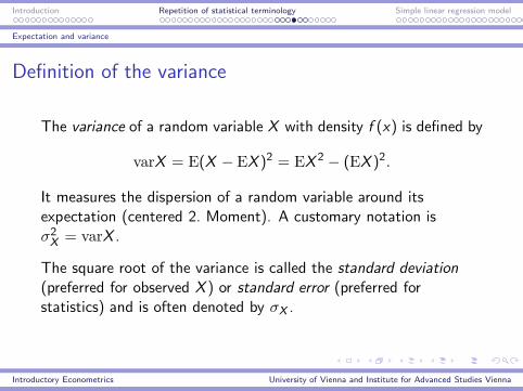
Definition of the variance
The variance of a random variable X with density f (x) is defined by
varX = E(X − EX )2 = EX 2 − (EX )2.
It measures the dispersion of a random variable around itsexpectation (centered 2. Moment). A customary notation isσ2X = varX .
The square root of the variance is called the standard deviation
(preferred for observed X ) or standard error (preferred forstatistics) and is often denoted by σX .
Introductory Econometrics University of Vienna and Institute for Advanced Studies Vienna
Introduction Repetition of statistical terminology Simple linear regression model
Expectation and variance
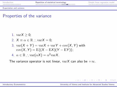
Properties of the variance
1. varX ≥ 0;
2. X ≡ α ∈ R ∴ varX = 0;
3. var(X + Y ) = varX + varY + cov(X ,Y ) withcov(X ,Y ) = E{(X − EX )(Y − EY )};
4. α ∈ R ∴ var(αX ) = α2varX .
The variance operator is not linear, varX can also be +∞.
Introductory Econometrics University of Vienna and Institute for Advanced Studies Vienna
Introduction Repetition of statistical terminology Simple linear regression model
Expectation and variance
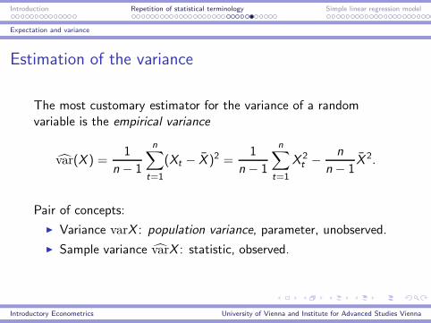
Estimation of the variance
The most customary estimator for the variance of a randomvariable is the empirical variance
var(X ) =1
n − 1
n∑
t=1
(Xt − X )2 =1
n− 1
n∑
t=1
X 2t −
n
n− 1X 2.
Pair of concepts:
◮ Variance varX : population variance, parameter, unobserved.
◮ Sample variance varX : statistic, observed.
Introductory Econometrics University of Vienna and Institute for Advanced Studies Vienna
Introduction Repetition of statistical terminology Simple linear regression model
Properties of estimators
Bias of estimators
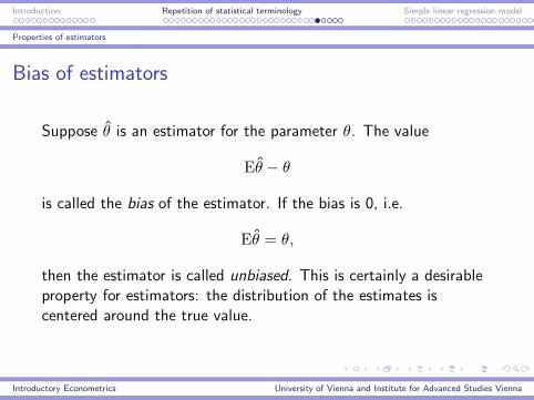
Suppose θ is an estimator for the parameter θ. The value
Eθ − θ
is called the bias of the estimator. If the bias is 0, i.e.
Eθ = θ,
then the estimator is called unbiased. This is certainly a desirableproperty for estimators: the distribution of the estimates iscentered around the true value.
Introductory Econometrics University of Vienna and Institute for Advanced Studies Vienna
Introduction Repetition of statistical terminology Simple linear regression model
Properties of estimators
Consistency of estimators
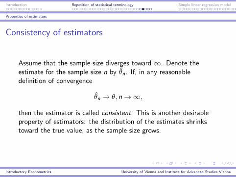
Assume that the sample size diverges toward ∞. Denote theestimate for the sample size n by θn. If, in any reasonabledefinition of convergence
θn → θ, n → ∞,
then the estimator is called consistent. This is another desirableproperty of estimators: the distribution of the estimates shrinkstoward the true value, as the sample size grows.
Introductory Econometrics University of Vienna and Institute for Advanced Studies Vienna
Introduction Repetition of statistical terminology Simple linear regression model
Properties of estimators
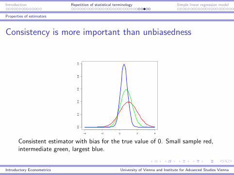
Consistency is more important than unbiasedness
−4 −2 0 2 4
0.0
0.2
0.4
0.6
0.8
1.0
Consistent estimator with bias for the true value of 0. Small sample red,intermediate green, largest blue.
Introductory Econometrics University of Vienna and Institute for Advanced Studies Vienna
Introduction Repetition of statistical terminology Simple linear regression model
Properties of estimators
Consistency and unbiasedness do not imply each other
Example: Let Xt be independently drawn from N(a,1). Someonebelieves a priori b to be a plausible value for the expectation.a1 = X + b/n is consistent, usually biased, and a reasonableestimator.
Example: Same assumptions, a2 = (X1 + Xn)/2 is unbiased, butinconsistent and an implausible estimator.
These examples are constructed but typical: inconsistent estimatorsshould be discarded, biased estimators can be useful or inevitable.
Introductory Econometrics University of Vienna and Institute for Advanced Studies Vienna
Introduction Repetition of statistical terminology Simple linear regression model
Properties of estimators
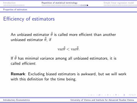
Efficiency of estimators
An unbiased estimator θ is called more efficient than anotherunbiased estimator θ, if
varθ < varθ.
If θ has minimal variance among all unbiased estimators, it iscalled efficient.
Remark: Excluding biased estimators is awkward, but we will workwith this definition for the time being.
Introductory Econometrics University of Vienna and Institute for Advanced Studies Vienna
Introduction Repetition of statistical terminology Simple linear regression model
Simple linear regression
The model explains (describes) a variable Y by a variable X , withn observations available for each of the two:
yt = α+ βxt + ut , t = 1, . . . , n,
where α and β are unknown parameters (coefficients). Theregression is called
◮ simple, as only one variable is used to explain Y ;
◮ linear, as the dependence of Y on X is modelled by a linear(affine) function.
Introductory Econometrics University of Vienna and Institute for Advanced Studies Vienna
Introduction Repetition of statistical terminology Simple linear regression model
Terminology
In words, Y is said to be regressed on X .
Y is called the dependent variable of the regression, also theregressand, the explained variable, the response;
X is called the explanatory variable of the regression, also theregressor, the design variable, the covariate.
Usage of the wording ‘independent variable’ for X is stronglydiscouraged. Only in true experiments will X be set independently.In the important multiple regression model, typically all regressorsare mutually dependent.
Introductory Econometrics University of Vienna and Institute for Advanced Studies Vienna
Introduction Repetition of statistical terminology Simple linear regression model
α and β
α is the intercept of the regression or the regression constant. Itrepresents the value for x = 0 on the theoretical regression liney = α+ βx , i.e. the location where the regression line intersectsthe y–axis. Example: in the consumption function, α isautonomous consumption.
β is the regression coefficient of X and indicates the marginalreaction of Y on changes in X an. It is the slope of the theoreticalregression line. Example: in the consumption function, β is themarginal propensity to consume.
Introductory Econometrics University of Vienna and Institute for Advanced Studies Vienna
Introduction Repetition of statistical terminology Simple linear regression model
What is u?
In the descriptive regression model, u is simply the unexplainedremainder.
In the statistical regression model, the true ut is an unobservedrandom variable, the error or disturbance term of the regression.
The word ‘residuals’ describes the observed(!) errors that evolveafter estimating coefficients. Some authors, however, call theunobserved errors ut ‘true residuals’.
Introductory Econometrics University of Vienna and Institute for Advanced Studies Vienna
Introduction Repetition of statistical terminology Simple linear regression model
Is simple regression an important model?
The simple linear regression model offers hardly anything newrelative to correlation analysis for two variables, and it is ratheruninteresting.
It is a didactic tool that permits to introduce new concepts thatcontinue to exist in the multiple regression model. This multiplemodel is the most important model of empirical economics.
Introductory Econometrics University of Vienna and Institute for Advanced Studies Vienna
Introduction Repetition of statistical terminology Simple linear regression model
The descriptive linear regression problem
Descriptive regression
The descriptive problem does not make any assumptions on thestatistical properties of variables and errors. It does not admit anystatistical conclusions.
The descriptive linear regression problem is to fit a straight linethrough a scatter of points, such that it fits as well as possible.
Introductory Econometrics University of Vienna and Institute for Advanced Studies Vienna
Introduction Repetition of statistical terminology Simple linear regression model
The descriptive linear regression problem
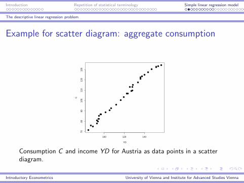
Example for scatter diagram: aggregate consumption
100 120 140
7080
9010
011
012
013
0
YD
C
Consumption C and income YD for Austria as data points in a scatterdiagram.
Introductory Econometrics University of Vienna and Institute for Advanced Studies Vienna
Introduction Repetition of statistical terminology Simple linear regression model
The descriptive linear regression problem
Suggestions how to fit a line through a scatter
1. The line should hit as many points as possible exactly:usually, the number of points that can be forced to lie on theline is just two;
2. ‘Free-hand method’: subjective;
3. Minimize distances (of line to points) in the plane: orthogonalregression, important but rarely used method. Variables aretreated symmetrically, like in correlation analysis;
4. Minimize the sum of vertical absolute distances: leastabsolute deviations (LAD). Robust procedure;
5. Minimize the sum of vertical squared distances: ordinary least
squares (OLS). Most commonly used method.
Introductory Econometrics University of Vienna and Institute for Advanced Studies Vienna
Introduction Repetition of statistical terminology Simple linear regression model
The descriptive linear regression problem
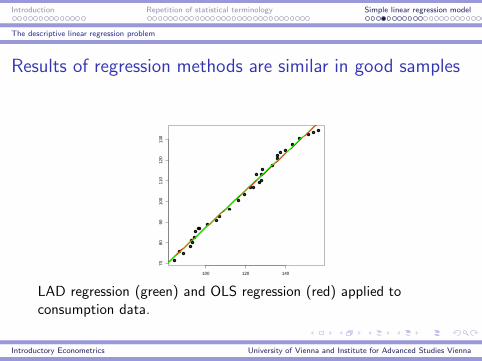
Results of regression methods are similar in good samples
100 120 140
7080
9010
011
012
013
0
LAD regression (green) and OLS regression (red) applied toconsumption data.
Introductory Econometrics University of Vienna and Institute for Advanced Studies Vienna
Introduction Repetition of statistical terminology Simple linear regression model
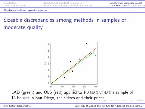
The descriptive linear regression problem
Sizeable discrepancies among methods in samples of
moderate quality
1000 1500 2000 2500 3000
200
250
300
350
400
450
500
Size
Pric
e
LAD (green) and OLS (red) applied to Ramanathan’s sample of14 houses in San Diego, their sizes and their prices.
Introductory Econometrics University of Vienna and Institute for Advanced Studies Vienna
Introduction Repetition of statistical terminology Simple linear regression model
The descriptive linear regression problem
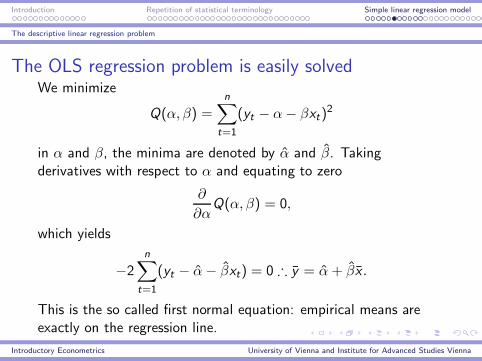
The OLS regression problem is easily solvedWe minimize
Q(α, β) =
n∑
t=1
(yt − α− βxt)2
in α and β, the minima are denoted by α and β. Takingderivatives with respect to α and equating to zero
∂
∂αQ(α, β) = 0,
which yields
−2n∑
t=1
(yt − α− βxt) = 0 ∴ y = α+ βx .
This is the so called first normal equation: empirical means areexactly on the regression line.
Introductory Econometrics University of Vienna and Institute for Advanced Studies Vienna
Introduction Repetition of statistical terminology Simple linear regression model
The descriptive linear regression problem
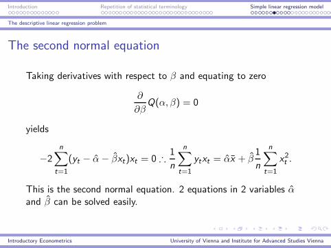
The second normal equation
Taking derivatives with respect to β and equating to zero
∂
∂βQ(α, β) = 0
yields
−2
n∑
t=1
(yt − α− βxt)xt = 0 ∴1
n
n∑
t=1
ytxt = αx + β1
n
n∑
t=1
x2t .
This is the second normal equation. 2 equations in 2 variables αand β can be solved easily.
Introductory Econometrics University of Vienna and Institute for Advanced Studies Vienna
Introduction Repetition of statistical terminology Simple linear regression model
The descriptive linear regression problem
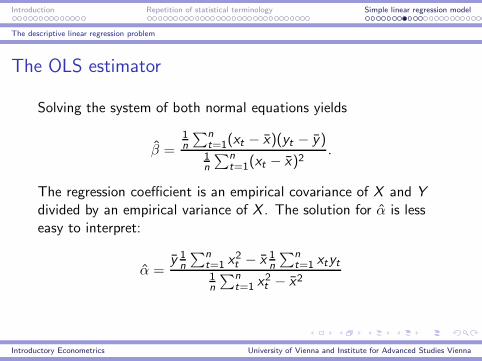
The OLS estimator
Solving the system of both normal equations yields
β =1n
∑nt=1(xt − x)(yt − y)1n
∑nt=1(xt − x)2
.
The regression coefficient is an empirical covariance of X and Y
divided by an empirical variance of X . The solution for α is lesseasy to interpret:
α =y 1n
∑nt=1 x
2t − x 1
n
∑nt=1 xtyt
1n
∑nt=1 x
2t − x2
Introductory Econometrics University of Vienna and Institute for Advanced Studies Vienna
Introduction Repetition of statistical terminology Simple linear regression model
The descriptive linear regression problem
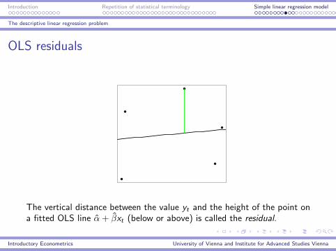
OLS residuals
The vertical distance between the value yt and the height of the point ona fitted OLS line α+ βxt (below or above) is called the residual.
Introductory Econometrics University of Vienna and Institute for Advanced Studies Vienna
Introduction Repetition of statistical terminology Simple linear regression model
The descriptive linear regression problem
Scatter diagrams
Scatter plots) with dependent variable on the y–axis and regressoron the x–axis are an important graphic tool in simple regression.
Because a linear regression function is fitted to the data, a linear
relationship should be recognizable.
Introductory Econometrics University of Vienna and Institute for Advanced Studies Vienna
Introduction Repetition of statistical terminology Simple linear regression model
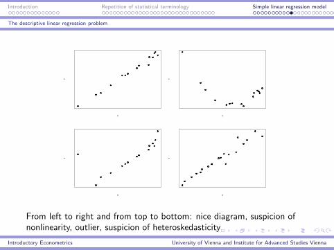
The descriptive linear regression problem
X
Y
X
Y
X
Y
X
Y
From left to right and from top to bottom: nice diagram, suspicion ofnonlinearity, outlier, suspicion of heteroskedasticity
Introductory Econometrics University of Vienna and Institute for Advanced Studies Vienna
Introduction Repetition of statistical terminology Simple linear regression model
The stochastic linear regression model
Stochastic linear regression: the idea
In the classical regression model
yt = α+ βxt + ut ,
a non-random input X impacts on an output Y and is disturbed bythe random variable U. Thus, also Y becomes a random variable.
Assumptions on the ‘design’ X and the statistical properties of Uadmit statistical statements on estimators and tests.
Introductory Econometrics University of Vienna and Institute for Advanced Studies Vienna
Introduction Repetition of statistical terminology Simple linear regression model
The stochastic linear regression model
Stochastic linear regression: critique
X as well as Y are typically observational data, there is noexperimental situation. Should not both X and Y be modelled asrandom variables and assumptions be imposed on these two?
In principle, this critique is justified. It is, however, didacticallysimpler to start with this simple model, and to generalize andmodify it later. So called fully stochastic models often userestrictive assumptions on the independence of observations.
Introductory Econometrics University of Vienna and Institute for Advanced Studies Vienna
Introduction Repetition of statistical terminology Simple linear regression model
The stochastic linear regression model
Assumption 1: Linearity of the model
Assumption 1. The observations correspond to the linear model
yt = α+ βxt + ut , t = 1, . . . , n.
Conceptually, this assumption is void without further assumptionson the errors ut .
Empirical consequence: nonlinear relationships often become linearafter transformations of X and/or Y .
Introductory Econometrics University of Vienna and Institute for Advanced Studies Vienna
Introduction Repetition of statistical terminology Simple linear regression model
The stochastic linear regression model
Assumption 2: Reasonable design
Assumption 2. Not all observed values for Xt are identical.
Experiments on the effect of X on Y are only meaningful if Xvaries. One observation is insufficient. Vertical regression lines areundesirable. Convenient: this assumption can be checkedimmediately by a simple inspection of the data (without anyhypothesis tests and exactly).
Introductory Econometrics University of Vienna and Institute for Advanced Studies Vienna
Introduction Repetition of statistical terminology Simple linear regression model
The stochastic linear regression model
Assumption 3: Stochastic errors
Assumption 3. The errors ut are realizations of random variablesUt , and it should also hold that
EUt = 0 ∀t.
Actually, these are 2 assumptions: U is an unobserved randomvariable, and its expectation is 0. Admitting an expectationunequal 0 would be meaningless, as then the regression constantwould not be defined (not identified).
Introductory Econometrics University of Vienna and Institute for Advanced Studies Vienna
Introduction Repetition of statistical terminology Simple linear regression model
The stochastic linear regression model
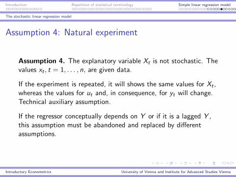
Assumption 4: Natural experiment
Assumption 4. The explanatory variable Xt is not stochastic. Thevalues xt , t = 1, . . . , n, are given data.
If the experiment is repeated, it will shows the same values for Xt ,whereas the values for ut and, in consequence, for yt will change.Technical auxiliary assumption.
If the regressor conceptually depends on Y or if it is a lagged Y ,this assumption must be abandoned and replaced by differentassumptions.
Introductory Econometrics University of Vienna and Institute for Advanced Studies Vienna
Introduction Repetition of statistical terminology Simple linear regression model
The stochastic linear regression model
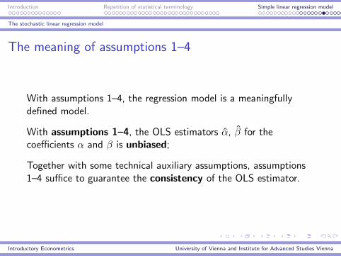
The meaning of assumptions 1–4
With assumptions 1–4, the regression model is a meaningfullydefined model.
With assumptions 1–4, the OLS estimators α, β for thecoefficients α and β is unbiased;
Together with some technical auxiliary assumptions, assumptions1–4 suffice to guarantee the consistency of the OLS estimator.
Introductory Econometrics University of Vienna and Institute for Advanced Studies Vienna
Introduction Repetition of statistical terminology Simple linear regression model
The stochastic linear regression model
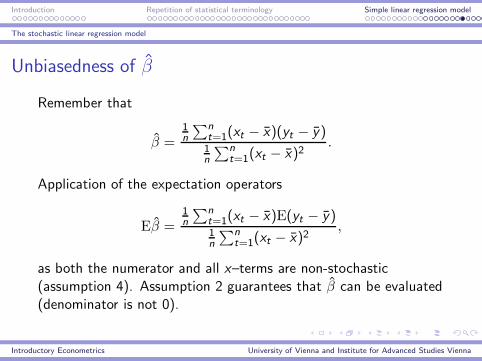
Unbiasedness of β
Remember that
β =1n
∑nt=1(xt − x)(yt − y)1n
∑nt=1(xt − x)2
.
Application of the expectation operators
Eβ =1n
∑nt=1(xt − x)E(yt − y)1n
∑nt=1(xt − x)2
,
as both the numerator and all x–terms are non-stochastic(assumption 4). Assumption 2 guarantees that β can be evaluated(denominator is not 0).
Introductory Econometrics University of Vienna and Institute for Advanced Studies Vienna
Introduction Repetition of statistical terminology Simple linear regression model
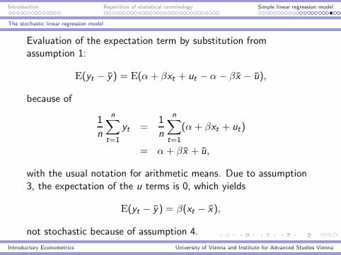
The stochastic linear regression model
Evaluation of the expectation term by substitution fromassumption 1:
E(yt − y) = E(α+ βxt + ut − α− βx − u),
because of
1
n
n∑
t=1
yt =1
n
n∑
t=1
(α+ βxt + ut)
= α+ βx + u,
with the usual notation for arithmetic means. Due to assumption3, the expectation of the u terms is 0, which yields
E(yt − y) = β(xt − x),
not stochastic because of assumption 4.
Introductory Econometrics University of Vienna and Institute for Advanced Studies Vienna
Introduction Repetition of statistical terminology Simple linear regression model
The stochastic linear regression model
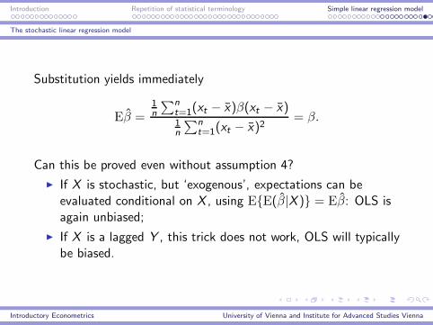
Substitution yields immediately
Eβ =1n
∑nt=1(xt − x)β(xt − x)1n
∑nt=1(xt − x)2
= β.
Can this be proved even without assumption 4?
◮ If X is stochastic, but ‘exogenous’, expectations can beevaluated conditional on X , using E{E(β|X )} = Eβ: OLS isagain unbiased;
◮ If X is a lagged Y , this trick does not work, OLS will typicallybe biased.
Introductory Econometrics University of Vienna and Institute for Advanced Studies Vienna
Introduction Repetition of statistical terminology Simple linear regression model
The stochastic linear regression model
Unbiasedness of α
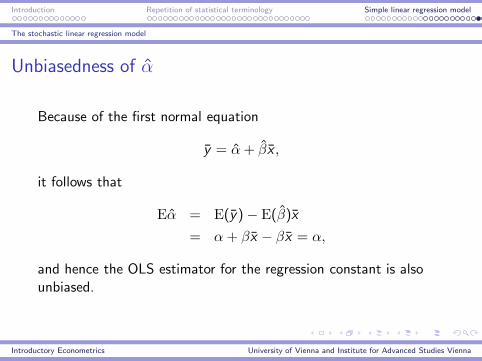
Because of the first normal equation
y = α+ βx ,
it follows that
Eα = E(y)− E(β)x
= α+ βx − βx = α,
and hence the OLS estimator for the regression constant is alsounbiased.
Introductory Econometrics University of Vienna and Institute for Advanced Studies Vienna
Introduction Repetition of statistical terminology Simple linear regression model
The stochastic linear regression model
Consistency of β
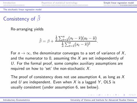
Re-arranging yields
β = β +1n
∑nt=1(xt − x)(ut − u)1n
∑nt=1(xt − x)2
.
For n → ∞, the denominator converges to a sort of variance of X ,and the numerator to 0, assuming the X are set independently ofU. For the formal proof, some complex auxiliary assumptions arerequired on how to ‘set’ the non-stochastic X .
The proof of consistency does not use assumption 4, as long as Xand U are independent. Even when X is a lagged Y , OLS isusually consistent (under assumption 6, see below).
Introductory Econometrics University of Vienna and Institute for Advanced Studies Vienna
Introduction Repetition of statistical terminology Simple linear regression model
The stochastic linear regression model
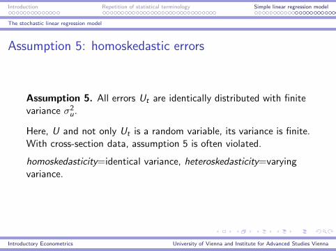
Assumption 5: homoskedastic errors
Assumption 5. All errors Ut are identically distributed with finitevariance σ2
u.
Here, U and not only Ut is a random variable, its variance is finite.With cross-section data, assumption 5 is often violated.
homoskedasticity=identical variance, heteroskedasticity=varyingvariance.
Introductory Econometrics University of Vienna and Institute for Advanced Studies Vienna
Introduction Repetition of statistical terminology Simple linear regression model
The stochastic linear regression model
Assumption 6: independent errors
Assumption 6. The errors Ut are statistically independent.
If the variance of Ut is finite, it follows that the Ut are alsouncorrelated (no autocorrelation). With time-series data,assumption 6 is often violated. Autocorrelation = correlation of avariable over time ‘with itself’ (auto).
Common mistake: Not the residuals ut are independent, but theerrors ut . OLS residuals are usually (slightly) autocorrelated.
Introductory Econometrics University of Vienna and Institute for Advanced Studies Vienna
Introduction Repetition of statistical terminology Simple linear regression model
The stochastic linear regression model
OLS becomes linear efficient
Assumptions 1–6 imply that the OLS estimators α and β are thelinear unbiased estimators with the smallest variance (o.c.s.).BLUE=best linear unbiased estimator.
A linear estimator can be represented as a linear combination of yt ,and this also holds for OLS. OLS is not necessarily the bestestimator (efficient).
This BLUE property (not shown here) under assumptions 1–6 isalso called the Gauss-Markov Theorem.
Introductory Econometrics University of Vienna and Institute for Advanced Studies Vienna
Introduction Repetition of statistical terminology Simple linear regression model
The stochastic linear regression model
Assumption 7: sample sufficiently large
Assumption 7. The sample must be larger than the number ofestimated regression coefficients.
The simple model has 2 coefficients, thus the sample should haveat least 3 observations. Fitting a straight line through 2 pointsexactly does not admit any inference on errors. Technicallyconvenient assumption: can be checked without any hypothesistests, just by counting.
Introductory Econometrics University of Vienna and Institute for Advanced Studies Vienna
Introduction Repetition of statistical terminology Simple linear regression model
The stochastic linear regression model
Assumption 8: normal regression
Assumption 8. All errors Ut are normally distributed.
It is convenient if the world is normally distributed, but is itrealistic? In small samples, it is impossible to test this assumption.In large samples, there is often evidence of it being violated.Regression under assumption 8 is called normal regression.
Introductory Econometrics University of Vienna and Institute for Advanced Studies Vienna
Introduction Repetition of statistical terminology Simple linear regression model
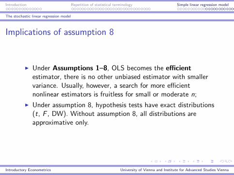
The stochastic linear regression model
Implications of assumption 8
◮ Under Assumptions 1–8, OLS becomes the efficient
estimator, there is no other unbiased estimator with smallervariance. Usually, however, a search for more efficientnonlinear estimators is fruitless for small or moderate n;
◮ Under assumption 8, hypothesis tests have exact distributions(t, F , DW). Without assumption 8, all distributions areapproximative only.
Introductory Econometrics University of Vienna and Institute for Advanced Studies Vienna
Introduction Repetition of statistical terminology Simple linear regression model
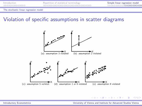
The stochastic linear regression model
Violation of specific assumptions in scatter diagrams
-X
6Y
������
••••
• ••••
••••••••
-X
6Y
������
•••
•
•
•
••
(a): assumption 3 violated (b): assumption 2 violated
-X
6Y
������
••
••
• ••
••
•
•
•
••
•
•
•
•
•
•
•
-X
6Y
������
••••••
•
••
••
•••••••
•
-X
6Y
������
•
•
•
•
•
•
•
•
•
•
•
•
•
•
•
•
•
•
•
•
•
•
•
•
•
•
•
•
•
•
•
•
•
•
(c): assumption 5 verletzt (d): assumption 1 or 6 violated (e): assumption 8 violated
Introductory Econometrics University of Vienna and Institute for Advanced Studies Vienna
Introduction Repetition of statistical terminology Simple linear regression model
Variances and covariances of the OLS estimator
The variance von β
Under assumptions 1–6, OLS is the BLUE estimator with smallestvariance. For β, this variance is given by
var(β) =σ2u
nvar∗(X )
,
using the n–weighted empirical variance of X
var∗(X ) =
1
n
n∑
t=1
(xt − x)2.
Proof by direct evaluation of expectation operators. Assumptions 5and 6 are used in the proof.
Introductory Econometrics University of Vienna and Institute for Advanced Studies Vienna
Introduction Repetition of statistical terminology Simple linear regression model
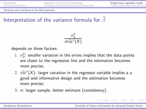
Variances and covariances of the OLS estimator
Interpretation of the variance formula for β
σ2u
nvar∗(X )
depends on three factors:
1. σ2u: smaller variation in the errors implies that the data points
are closer to the regression line and the estimation becomesmore precise;
2. var∗(X ): larger variation in the regressor variable implies a a
good and informative design and the estimation becomesmore precise;
3. n: larger sample, better estimate (consistency).
Introductory Econometrics University of Vienna and Institute for Advanced Studies Vienna
Introduction Repetition of statistical terminology Simple linear regression model
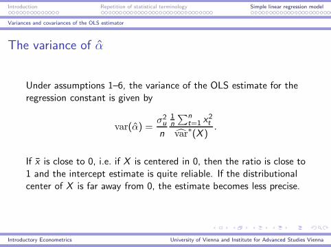
Variances and covariances of the OLS estimator
The variance of α
Under assumptions 1–6, the variance of the OLS estimate for theregression constant is given by
var(α) =σ2u
n
1n
∑nt=1 x
2t
var∗(X )
.
If x is close to 0, i.e. if X is centered in 0, then the ratio is close to1 and the intercept estimate is quite reliable. If the distributionalcenter of X is far away from 0, the estimate becomes less precise.
Introductory Econometrics University of Vienna and Institute for Advanced Studies Vienna
Introduction Repetition of statistical terminology Simple linear regression model
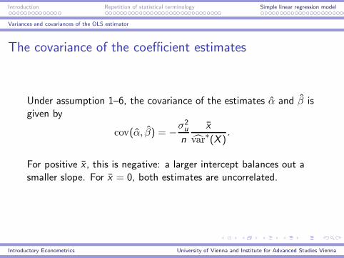
Variances and covariances of the OLS estimator
The covariance of the coefficient estimates
Under assumption 1–6, the covariance of the estimates α and β isgiven by
cov(α, β) = −σ2u
n
x
var∗(X )
.
For positive x , this is negative: a larger intercept balances out asmaller slope. For x = 0, both estimates are uncorrelated.
Introductory Econometrics University of Vienna and Institute for Advanced Studies Vienna
Introduction Repetition of statistical terminology Simple linear regression model
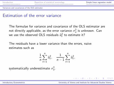
Variances and covariances of the OLS estimator
Estimation of the error variance
The formulae for variance and covariance of the OLS estimator arenot directly applicable, as the error variance σ2
u is unknown. Canwe use the observed OLS residuals u2t to estimate it?
The residuals have a lower variance than the errors, naiveestimates such as
1
n
n∑
t=1
u2t ,1
n− 1
n∑
t=1
u2t ,
systematically underestimate σ2u.
Introductory Econometrics University of Vienna and Institute for Advanced Studies Vienna
Introduction Repetition of statistical terminology Simple linear regression model
Variances and covariances of the OLS estimator
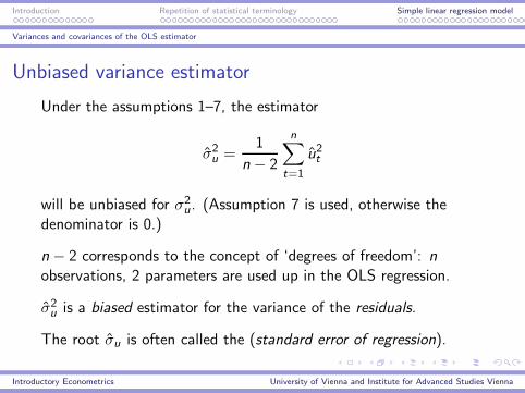
Unbiased variance estimator
Under the assumptions 1–7, the estimator
σ2u =
1
n− 2
n∑
t=1
u2t
will be unbiased for σ2u. (Assumption 7 is used, otherwise the
denominator is 0.)
n − 2 corresponds to the concept of ‘degrees of freedom’: nobservations, 2 parameters are used up in the OLS regression.
σ2u is a biased estimator for the variance of the residuals.
The root σu is often called the (standard error of regression).
Introductory Econometrics University of Vienna and Institute for Advanced Studies Vienna
Introduction Repetition of statistical terminology Simple linear regression model
Variances and covariances of the OLS estimator
Standard errors of regression coefficients
The feasible variance estimate of β is
σ2β =
σ2u
nvar∗(X )
,
which, under assumptions 1–7, provides an unbiased estimate forvarβ = σ2
β. An analogous argument applies to σ2α and to the
covariance.
The standard error or the estimated standard deviation is thesquare root of this value. This estimator is not unbiased for σβ.
Introductory Econometrics University of Vienna and Institute for Advanced Studies Vienna
Introduction Repetition of statistical terminology Simple linear regression model
Homogeneous linear regression
Homogeneous linear regression
Sometimes, it may look attractive (for empirical or theoreticalreasons) to constrain the inhomogeneous regression
yt = α+ βxt + ut
and to replace it by the homogeneous regression,
yt = βxt + ut
which forces the regression line through the origin.
Introductory Econometrics University of Vienna and Institute for Advanced Studies Vienna
Introduction Repetition of statistical terminology Simple linear regression model
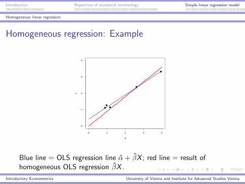
Homogeneous linear regression
Homogeneous regression: Example
0 1 2 3 4
01
23
4
X
Y
Blue line = OLS regression line α+ βX ; red line = result ofhomogeneous OLS regression βX .
Introductory Econometrics University of Vienna and Institute for Advanced Studies Vienna
Introduction Repetition of statistical terminology Simple linear regression model
Homogeneous linear regression
The homogeneous OLS estimator
The task to minimize the sum of squared vertical distance underthe constraint that the regression line passes through the origin,can be written in symbols
minQ0(β) =
n∑
t=1
(yt − βxt)2,
which yields the solution
β =
∑nt=1 xtyt∑nt=1 x
2t
.
Introductory Econometrics University of Vienna and Institute for Advanced Studies Vienna
Introduction Repetition of statistical terminology Simple linear regression model
Homogeneous linear regression
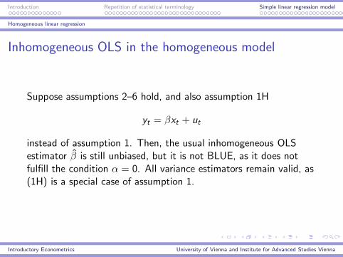
Inhomogeneous OLS in the homogeneous model
Suppose assumptions 2–6 hold, and also assumption 1H
yt = βxt + ut
instead of assumption 1. Then, the usual inhomogeneous OLSestimator β is still unbiased, but it is not BLUE, as it does notfulfill the condition α = 0. All variance estimators remain valid, as(1H) is a special case of assumption 1.
Introductory Econometrics University of Vienna and Institute for Advanced Studies Vienna
Introduction Repetition of statistical terminology Simple linear regression model
Homogeneous linear regression
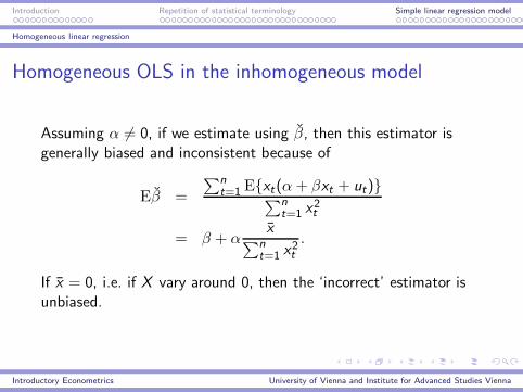
Homogeneous OLS in the inhomogeneous model
Assuming α 6= 0, if we estimate using β, then this estimator isgenerally biased and inconsistent because of
Eβ =
∑nt=1 E{xt(α+ βxt + ut)}∑n
t=1 x2t
= β + αx∑n
t=1 x2t
.
If x = 0, i.e. if X vary around 0, then the ‘incorrect’ estimator isunbiased.
Introductory Econometrics University of Vienna and Institute for Advanced Studies Vienna
Introduction Repetition of statistical terminology Simple linear regression model
Homogeneous linear regression
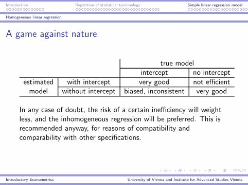
A game against nature
true modelintercept no intercept
estimated with intercept very good not efficientmodel without intercept biased, inconsistent very good
In any case of doubt, the risk of a certain inefficiency will weightless, and the inhomogeneous regression will be preferred. This isrecommended anyway, for reasons of compatibility andcomparability with other specifications.
Introductory Econometrics University of Vienna and Institute for Advanced Studies Vienna
Introduction Repetition of statistical terminology Simple linear regression model
The t–test
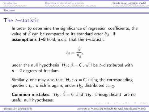
The t–statisticIn order to determine the significance of regression coefficients, thevalue of β can be compared to its standard error σβ. Ifassumptions 1–8 hold, o.c.s. that the t–statistic
tβ =β
σβ,
under the null hypothesis ‘H0 : β = 0’, will be t–distributed withn − 2 degrees of freedom.
Similarly, one may also test ‘H0 : α = 0’ using the correspondingquotient tα, which is again, under H0, distributed tn−2.
Common mistakes: ‘H0 : β = 0’ and ‘H0 : β insignificant’ are nouseful null hypotheses.
Introductory Econometrics University of Vienna and Institute for Advanced Studies Vienna
Introduction Repetition of statistical terminology Simple linear regression model
The t–test
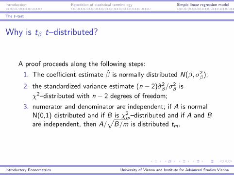
Why is tβ t–distributed?
A proof proceeds along the following steps:
1. The coefficient estimate β is normally distributed N(β, σ2β);
2. the standardized variance estimate (n − 2)σ2β/σ
2β is
χ2–distributed with n − 2 degrees of freedom;
3. numerator and denominator are independent; if A is normalN(0,1) distributed and if B is χ2
m–distributed and if A and B
are independent, then A/√
B/m is distributed tm.
Introductory Econometrics University of Vienna and Institute for Advanced Studies Vienna
Introduction Repetition of statistical terminology Simple linear regression model
The t–test
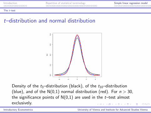
t–distribution and normal distribution
−4 −2 0 2 4
0.0
0.1
0.2
0.3
0.4
f(x)
Density of the t3–distribution (black), of the t10–distribution(blue), and of the N(0,1) normal distribution (red). For n > 30,the significance points of N(0,1) are used in the t–test almostexclusively.
Introductory Econometrics University of Vienna and Institute for Advanced Studies Vienna
Introduction Repetition of statistical terminology Simple linear regression model
The t–test
t–Test if assumption 8 is invalid
If assumption 8 does not hold and n is ‘large’, then the t–statisticis approximately normal N(0,1) distributed. Usually, n > 30 is seenas a criterion for large samples here.
Because the two-sided 5% points of the N(0,1) are around ±1.96,many empirical researchers use the t–statistic for a thumb-ruleevaluation only, in the sense that it is significant when it is greatertwo in absolute value.
If assumption 8 does not hold and the sample is small, then thet–test is unreliable.
Introductory Econometrics University of Vienna and Institute for Advanced Studies Vienna
Introduction Repetition of statistical terminology Simple linear regression model
The t–test
t–test on ‘H0 : β = β0’
One may be interested in testing whether β corresponds to aspecific pre-specified value (Example: if the propensity to consumeequals 1). The null hypothesis ‘H0 : β = β0’ is tested using thet–statistic
β − β0σβ
,
which again, under H0, is distributed tn−2.
This statistic is not supplied automatically, but it is easy todetermine from the formula tβ − β0/σβ .
Introductory Econometrics University of Vienna and Institute for Advanced Studies Vienna
Introduction Repetition of statistical terminology Simple linear regression model
The t–test
Statistical regression programs and the t–test
◮ Often, β, σβ, and the ratio tβ are supplied, increasingly eventhe p–value of the t–test;
◮ The software assumes assumptions 1–8 to hold and routinelyuses the t–distribution, even when assumption 8 is invalid:take care;
◮ The p–value refers to the two-sided test against ‘HA : β 6= 0’:for the one-sided test (for example ‘HA : β > 0’) you have toadjust.
Introductory Econometrics University of Vienna and Institute for Advanced Studies Vienna
Introduction Repetition of statistical terminology Simple linear regression model
Goodness of fit
Coefficient of determination: idea
One may be interested in a descriptive statistic that quantifies towhat degree Y is described linearly by X . The empirical coefficientof correlation
corr(X ,Y ) =1n
∑nt=1(xt − x)(yt − y)√
1n
∑nt=1(xt − x)2 1
n
∑nt=1(yt − y)2
does just that. For random variables(!) X and Y , it estimates thecorrelation
corr(X ,Y ) =cov(X ,Y )√var(X )var(Y )
,
which measures linear dependence. In regression analysis, it iscustomary to use the square of this statistic and to call it R2.
Introductory Econometrics University of Vienna and Institute for Advanced Studies Vienna
Introduction Repetition of statistical terminology Simple linear regression model
Goodness of fit
OLS decomposes the dependent variable
OLS estimation decomposes yt into an explained and anunexplained component:
yt = α+ βxt + ut = yt + ut .
ut is called the residual. yt is the systematic, explained part of yt ,and it is often called the predictor.
Introductory Econometrics University of Vienna and Institute for Advanced Studies Vienna
Introduction Repetition of statistical terminology Simple linear regression model
Goodness of fit
Variance decompositionThe second normal equation implies
n∑
t=1
xt ut = 0,
and, because of the first normal equation,∑n
t=1 ut = 0. It followsthat
cov(U,X ) =1
n
n∑
t=1
(ut − ¯u)(xt − x) = 0.
However, yt is only a linear transformation of xt , hence it isuncorrelated with the residuals. It follows that
n∑
t=1
(yt − y)2 =
n∑
t=1
(yt − y)2 +
n∑
t=1
u2t .
Introductory Econometrics University of Vienna and Institute for Advanced Studies Vienna
Introduction Repetition of statistical terminology Simple linear regression model
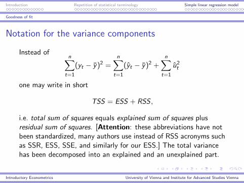
Goodness of fit
Notation for the variance components
Instead ofn∑
t=1
(yt − y)2 =n∑
t=1
(yt − y)2 +n∑
t=1
u2t
one may write in short
TSS = ESS + RSS ,
i.e. total sum of squares equals explained sum of squares plusresidual sum of squares. [Attention: these abbreviations have notbeen standardized, many authors use instead of RSS acronyms suchas SSR, ESS, SSE, and similarly for our ESS.] The total variancehas been decomposed into an explained and an unexplained part.
Introductory Econometrics University of Vienna and Institute for Advanced Studies Vienna
Introduction Repetition of statistical terminology Simple linear regression model
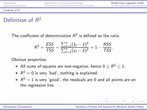
Goodness of fit
Definition of R2
The coefficient of determination R2 is defined as the ratio
R2 =ESS
TSS=
∑nt=1(yt − y)2∑nt=1(yt − y)2
= 1−RSS
TSS.
Obvious properties:
◮ All sums of squares are non-negative, hence 0 ≤ R2 ≤ 1;
◮ R2 = 0 is very ‘bad’, nothing is explained;
◮ R2 = 1 is very ‘good’, the residuals are 0 and all points are onthe regression line.
Introductory Econometrics University of Vienna and Institute for Advanced Studies Vienna
Introduction Repetition of statistical terminology Simple linear regression model
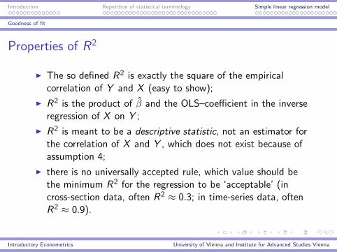
Goodness of fit
Properties of R2
◮ The so defined R2 is exactly the square of the empiricalcorrelation of Y and X (easy to show);
◮ R2 is the product of β and the OLS–coefficient in the inverseregression of X on Y ;
◮ R2 is meant to be a descriptive statistic, not an estimator forthe correlation of X and Y , which does not exist because ofassumption 4;
◮ there is no universally accepted rule, which value should bethe minimum R2 for the regression to be ‘acceptable’ (incross-section data, often R2 ≈ 0.3; in time-series data, oftenR2 ≈ 0.9).
Introductory Econometrics University of Vienna and Institute for Advanced Studies Vienna
Introduction Repetition of statistical terminology Simple linear regression model
Goodness of fit
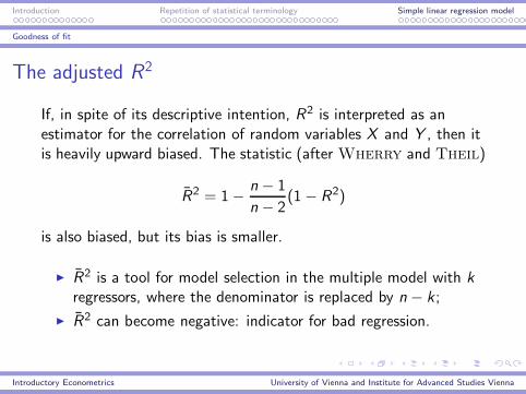
The adjusted R2
If, in spite of its descriptive intention, R2 is interpreted as anestimator for the correlation of random variables X and Y , then itis heavily upward biased. The statistic (after Wherry and Theil)
R2 = 1−n − 1
n − 2(1− R2)
is also biased, but its bias is smaller.
◮ R2 is a tool for model selection in the multiple model with k
regressors, where the denominator is replaced by n − k ;
◮ R2 can become negative: indicator for bad regression.
Introductory Econometrics University of Vienna and Institute for Advanced Studies Vienna
Introduction Repetition of statistical terminology Simple linear regression model
The F-total–test
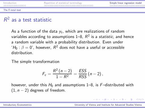
R2 as a test statistic
As a function of the data yt , which are realizations of randomvariables according to assumptions 1–8, R2 is a statistic, and hencea random variable with a probability distribution. Even under‘H0 : β = 0’, however, R2 does not have a useful or accessibledistribution.
The simple transformation
Fc =R2 (n − 2)
1− R2=
ESS
RSS(n− 2) ,
however, under this H0 and assumptions 1–8, is F–distributed with(1, n − 2) degrees of freedom.
Introductory Econometrics University of Vienna and Institute for Advanced Studies Vienna
Introduction Repetition of statistical terminology Simple linear regression model
The F-total–test
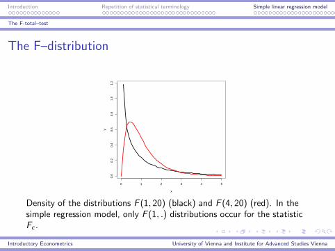
The F–distribution
0 1 2 3 4 5
0.0
0.2
0.4
0.6
0.8
1.0
1.2
x
y
Density of the distributions F (1, 20) (black) and F (4, 20) (red). In thesimple regression model, only F (1, .) distributions occur for the statisticFc .
Introductory Econometrics University of Vienna and Institute for Advanced Studies Vienna
Introduction Repetition of statistical terminology Simple linear regression model
The F-total–test
Why is Fc F (1, n − 2)–distributed?
◮ The F (m, n)–distribution after Snedecor (the ‘F’ honorsFisher) is the distribution of a random variable(A/m)/(B/n), if A and B are independent χ2–distributedwith m respectively n degree of freedom: therefore, numeratordegrees of freedom m and denominator degrees of freedom n;
◮ the explained and the unexplained shares ESS and RSS areindependent (because uncorrelated and assumption 8); underH0, ESS is χ2(1)–distributed, RSS is distributed χ2(n − 2);
◮ all F–distributions describe non-negative random variables,rejection of H0 at large values (always one-sided test).
Introductory Econometrics University of Vienna and Institute for Advanced Studies Vienna
Introduction Repetition of statistical terminology Simple linear regression model
The F-total–test
Fc in the simple regression model
◮ Fc is provided by all regression programs, often with p–value;
◮ the F-total–test tests the same H0 as the t–test for β, andeven Fc = t2β, thus Fc has no additional information in thesimple model;
◮ Fc becomes more important in the multiple model.
Introductory Econometrics University of Vienna and Institute for Advanced Studies Vienna