introduction to the logistic regression model · pdf filechapter 1 introduction to the...
TRANSCRIPT
C H A P T E R 1
Introduction to the LogisticRegression Model
1.1 INTRODUCTION
Regression methods have become an integral component of any data analysisconcerned with describing the relationship between a response variable and oneor more explanatory variables. Quite often the outcome variable is discrete, tak-ing on two or more possible values. The logistic regression model is the mostfrequently used regression model for the analysis of these data.
Before beginning a thorough study of the logistic regression model it is importantto understand that the goal of an analysis using this model is the same as that ofany other regression model used in statistics, that is, to find the best fitting and mostparsimonious, clinically interpretable model to describe the relationship betweenan outcome (dependent or response) variable and a set of independent (predictoror explanatory) variables. The independent variables are often called covariates.The most common example of modeling, and one assumed to be familiar to thereaders of this text, is the usual linear regression model where the outcome variableis assumed to be continuous.
What distinguishes a logistic regression model from the linear regression modelis that the outcome variable in logistic regression is binary or dichotomous. Thisdifference between logistic and linear regression is reflected both in the form ofthe model and its assumptions. Once this difference is accounted for, the methodsemployed in an analysis using logistic regression follow, more or less, the samegeneral principles used in linear regression. Thus, the techniques used in linearregression analysis motivate our approach to logistic regression. We illustrate boththe similarities and differences between logistic regression and linear regressionwith an example.
Applied Logistic Regression, Third Edition.David W. Hosmer, Jr., Stanley Lemeshow, and Rodney X. Sturdivant.© 2013 John Wiley & Sons, Inc. Published 2013 by John Wiley & Sons, Inc.
1
2 introduction to the logistic regression model
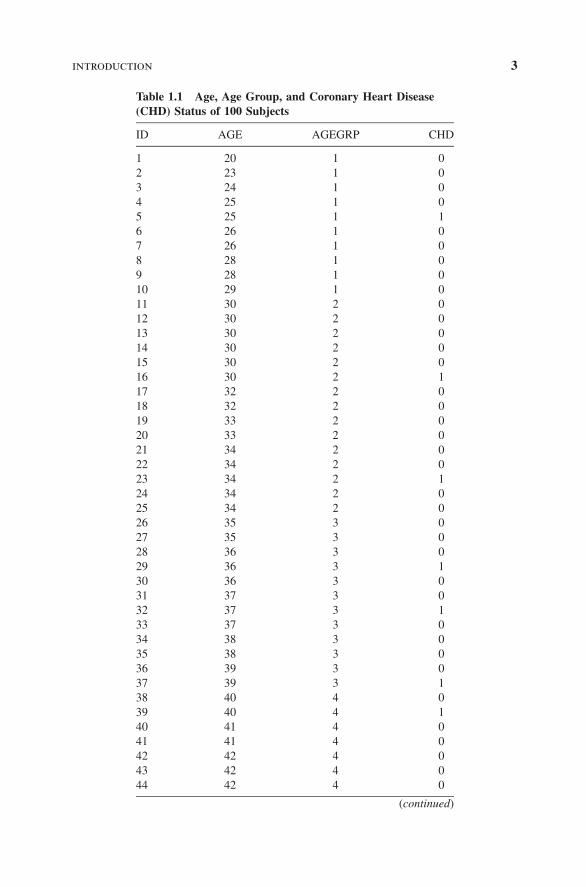
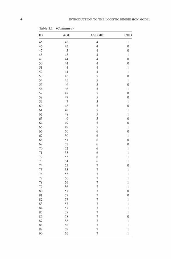
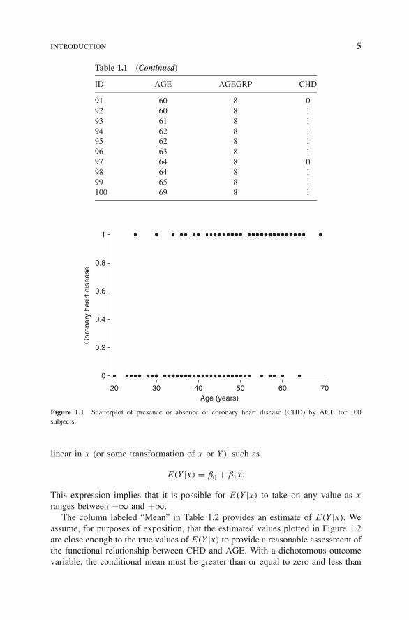
Example 1: Table 1.1 lists the age in years (AGE), and presence or absence ofevidence of significant coronary heart disease (CHD) for 100 subjects in a hypo-thetical study of risk factors for heart disease. The table also contains an identifiervariable (ID) and an age group variable (AGEGRP). The outcome variable is CHD,which is coded with a value of “0” to indicate that CHD is absent, or “1” to indicatethat it is present in the individual. In general, any two values could be used, butwe have found it most convenient to use zero and one. We refer to this data set asthe CHDAGE data.
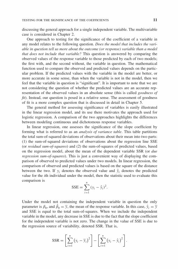
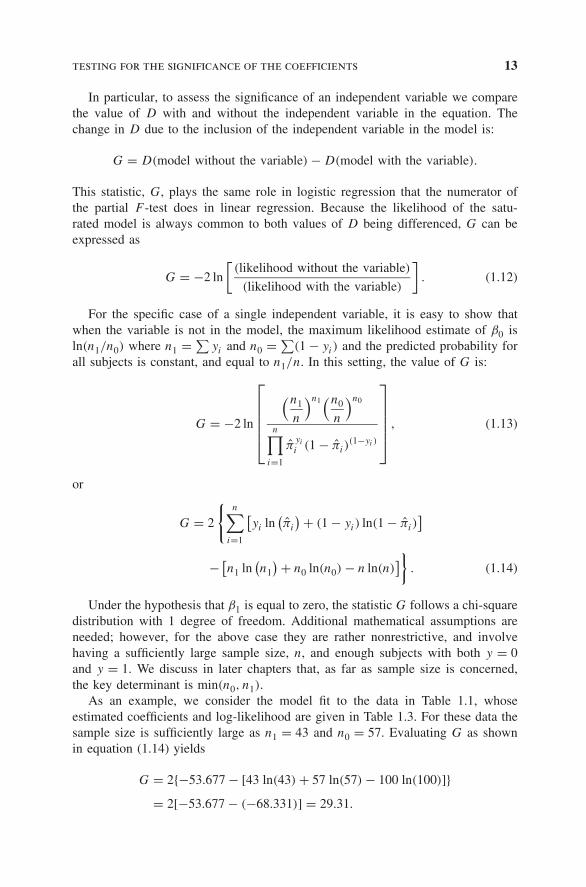
It is of interest to explore the relationship between AGE and the presence orabsence of CHD in this group. Had our outcome variable been continuous ratherthan binary, we probably would begin by forming a scatterplot of the outcomeversus the independent variable. We would use this scatterplot to provide an impres-sion of the nature and strength of any relationship between the outcome and theindependent variable. A scatterplot of the data in Table 1.1 is given in Figure 1.1.
In this scatterplot, all points fall on one of two parallel lines representing theabsence of CHD (y = 0) or the presence of CHD (y = 1). There is some tendencyfor the individuals with no evidence of CHD to be younger than those with evidenceof CHD. While this plot does depict the dichotomous nature of the outcome variablequite clearly, it does not provide a clear picture of the nature of the relationshipbetween CHD and AGE.
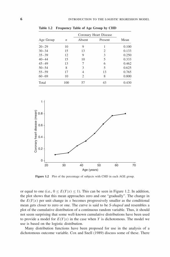
The main problem with Figure 1.1 is that the variability in CHD at all ages islarge. This makes it difficult to see any functional relationship between AGE andCHD. One common method of removing some variation, while still maintainingthe structure of the relationship between the outcome and the independent variable,is to create intervals for the independent variable and compute the mean of theoutcome variable within each group. We use this strategy by grouping age into thecategories (AGEGRP) defined in Table 1.1. Table 1.2 contains, for each age group,the frequency of occurrence of each outcome, as well as the percent with CHDpresent.
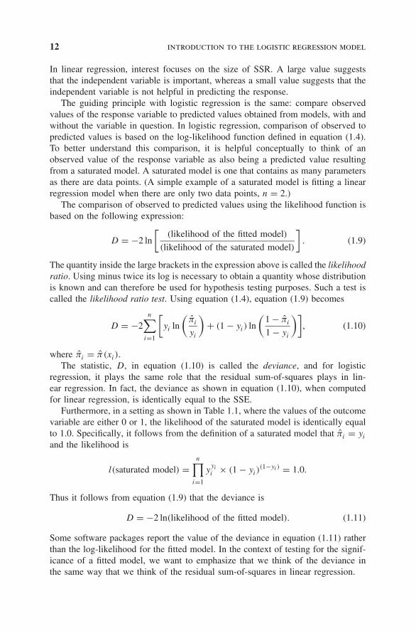
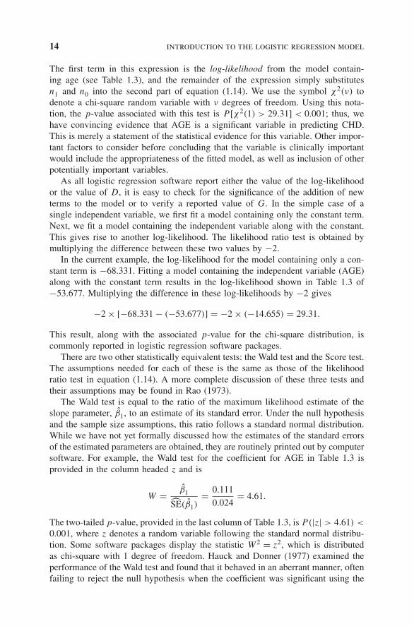
By examining this table, a clearer picture of the relationship begins to emerge. Itshows that as age increases, the proportion (mean) of individuals with evidence ofCHD increases. Figure 1.2 presents a plot of the percent of individuals with CHDversus the midpoint of each age interval. This plot provides considerable insightinto the relationship between CHD and AGE in this study, but the functional formfor this relationship needs to be described. The plot in this figure is similar to whatone might obtain if this same process of grouping and averaging were performedin a linear regression. We note two important differences.
The first difference concerns the nature of the relationship between the outcomeand independent variables. In any regression problem the key quantity is the meanvalue of the outcome variable, given the value of the independent variable. Thisquantity is called the conditional mean and is expressed as “E(Y |x)” where Y
denotes the outcome variable and x denotes a specific value of the independentvariable. The quantity E(Y |x) is read “the expected value of Y , given the value x”.In linear regression we assume that this mean may be expressed as an equation
introduction 3
Table 1.1 Age, Age Group, and Coronary Heart Disease(CHD) Status of 100 Subjects
ID AGE AGEGRP CHD
1 20 1 02 23 1 03 24 1 04 25 1 05 25 1 16 26 1 07 26 1 08 28 1 09 28 1 010 29 1 011 30 2 012 30 2 013 30 2 014 30 2 015 30 2 016 30 2 117 32 2 018 32 2 019 33 2 020 33 2 021 34 2 022 34 2 023 34 2 124 34 2 025 34 2 026 35 3 027 35 3 028 36 3 029 36 3 130 36 3 031 37 3 032 37 3 133 37 3 034 38 3 035 38 3 036 39 3 037 39 3 138 40 4 039 40 4 140 41 4 041 41 4 042 42 4 043 42 4 044 42 4 0
(continued)
4 introduction to the logistic regression model
Table 1.1 (Continued)
ID AGE AGEGRP CHD
45 42 4 146 43 4 047 43 4 048 43 4 149 44 4 050 44 4 051 44 4 152 44 4 153 45 5 054 45 5 155 46 5 056 46 5 157 47 5 058 47 5 059 47 5 160 48 5 061 48 5 162 48 5 163 49 5 064 49 5 065 49 5 166 50 6 067 50 6 168 51 6 069 52 6 070 52 6 171 53 6 172 53 6 173 54 6 174 55 7 075 55 7 176 55 7 177 56 7 178 56 7 179 56 7 180 57 7 081 57 7 082 57 7 183 57 7 184 57 7 185 57 7 186 58 7 087 58 7 188 58 7 189 59 7 190 59 7 1
introduction 5
Table 1.1 (Continued)
ID AGE AGEGRP CHD
91 60 8 092 60 8 193 61 8 194 62 8 195 62 8 196 63 8 197 64 8 098 64 8 199 65 8 1100 69 8 1
0
0.2
0.4
0.6
0.8
1
Cor
onar
y he
art d
isea
se
20 30 40 50 60 70Age (years)
Figure 1.1 Scatterplot of presence or absence of coronary heart disease (CHD) by AGE for 100subjects.
linear in x (or some transformation of x or Y ), such as
E(Y |x) = β0 + β1x.
This expression implies that it is possible for E(Y |x) to take on any value as x
ranges between −∞ and +∞.The column labeled “Mean” in Table 1.2 provides an estimate of E(Y |x). We
assume, for purposes of exposition, that the estimated values plotted in Figure 1.2are close enough to the true values of E(Y |x) to provide a reasonable assessment ofthe functional relationship between CHD and AGE. With a dichotomous outcomevariable, the conditional mean must be greater than or equal to zero and less than
6 introduction to the logistic regression model
Table 1.2 Frequency Table of Age Group by CHD
Coronary Heart Disease
Age Group n Absent Present Mean
20–29 10 9 1 0.10030–34 15 13 2 0.13335–39 12 9 3 0.25040–44 15 10 5 0.33345–49 13 7 6 0.46250–54 8 3 5 0.62555–59 17 4 13 0.76560–69 10 2 8 0.800
Total 100 57 43 0.430
0
0.2
0.4
0.6
0.8
1
Cor
onar
y he
art d
isea
se (
mea
n)
20 30 40 50 60 70
Age (years)
Figure 1.2 Plot of the percentage of subjects with CHD in each AGE group.
or equal to one (i.e., 0 ≤ E(Y |x) ≤ 1). This can be seen in Figure 1.2. In addition,the plot shows that this mean approaches zero and one “gradually”. The change inthe E(Y |x) per unit change in x becomes progressively smaller as the conditionalmean gets closer to zero or one. The curve is said to be S-shaped and resembles aplot of the cumulative distribution of a continuous random variable. Thus, it shouldnot seem surprising that some well-known cumulative distributions have been usedto provide a model for E(Y |x) in the case when Y is dichotomous. The model weuse is based on the logistic distribution.
Many distribution functions have been proposed for use in the analysis of adichotomous outcome variable. Cox and Snell (1989) discuss some of these. There
introduction 7
are two primary reasons for choosing the logistic distribution. First, from a mathe-matical point of view, it is an extremely flexible and easily used function. Second,its model parameters provide the basis for clinically meaningful estimates of effect.A detailed discussion of the interpretation of the model parameters is given inChapter 3.
In order to simplify notation, we use the quantity π(x) = E(Y |x) to representthe conditional mean of Y given x when the logistic distribution is used. Thespecific form of the logistic regression model we use is:
π(x) = eβ0+β1x
1 + eβ0+β1x. (1.1)
A transformation of π(x) that is central to our study of logistic regression is thelogit transformation. This transformation is defined, in terms of π(x), as:
g(x) = ln
[π (x)
1 − π(x)
]= β0 + β1x.
The importance of this transformation is that g(x) has many of the desirable prop-erties of a linear regression model. The logit, g(x), is linear in its parameters, maybe continuous, and may range from −∞ to +∞, depending on the range of x.
The second important difference between the linear and logistic regressionmodels concerns the conditional distribution of the outcome variable. In the linearregression model we assume that an observation of the outcome variable may beexpressed as y = E(Y |x) + ε. The quantity ε is called the error and expresses anobservation’s deviation from the conditional mean. The most common assumptionis that ε follows a normal distribution with mean zero and some variance that isconstant across levels of the independent variable. It follows that the conditionaldistribution of the outcome variable given x is normal with mean E(Y |x), and avariance that is constant. This is not the case with a dichotomous outcome vari-able. In this situation, we may express the value of the outcome variable given x
as y = π(x) + ε. Here the quantity ε may assume one of two possible values. Ify = 1 then ε = 1 − π(x) with probability π(x), and if y = 0 then ε = −π(x) withprobability 1 − π(x). Thus, ε has a distribution with mean zero and variance equalto π(x)[1 − π(x)]. That is, the conditional distribution of the outcome variablefollows a binomial distribution with probability given by the conditional mean,π(x).
In summary, we have shown that in a regression analysis when the outcomevariable is dichotomous:
1. The model for the conditional mean of the regression equation must bebounded between zero and one. The logistic regression model, π(x), givenin equation (1.1), satisfies this constraint.
2. The binomial, not the normal, distribution describes the distribution of theerrors and is the statistical distribution on which the analysis is based.
8 introduction to the logistic regression model
3. The principles that guide an analysis using linear regression also guide us inlogistic regression.
1.2 FITTING THE LOGISTIC REGRESSION MODEL
Suppose we have a sample of n independent observations of the pair (xi, yi),i = 1, 2, . . . , n, where yi denotes the value of a dichotomous outcome variable andxi is the value of the independent variable for the ith subject. Furthermore, assumethat the outcome variable has been coded as 0 or 1, representing the absence or thepresence of the characteristic, respectively. This coding for a dichotomous outcomeis used throughout the text. Fitting the logistic regression model in equation (1.1)to a set of data requires that we estimate the values of β0 and β1, the unknownparameters.
In linear regression, the method used most often for estimating unknown param-eters is least squares. In that method we choose those values of β0 and β1 thatminimize the sum-of-squared deviations of the observed values of Y from the pre-dicted values based on the model. Under the usual assumptions for linear regressionthe method of least squares yields estimators with a number of desirable statisticalproperties. Unfortunately, when the method of least squares is applied to a modelwith a dichotomous outcome, the estimators no longer have these same properties.
The general method of estimation that leads to the least squares function underthe linear regression model (when the error terms are normally distributed) iscalled maximum likelihood. This method provides the foundation for our approachto estimation with the logistic regression model throughout this text. In a generalsense, the method of maximum likelihood yields values for the unknown parametersthat maximize the probability of obtaining the observed set of data. In order to applythis method we must first construct a function, called the likelihood function. Thisfunction expresses the probability of the observed data as a function of the unknownparameters. The maximum likelihood estimators of the parameters are the valuesthat maximize this function. Thus, the resulting estimators are those that agree mostclosely with the observed data. We now describe how to find these values for thelogistic regression model.
If Y is coded as 0 or 1 then the expression for π(x) given in equation (1.1)provides (for an arbitrary value of β = (β0, β1), the vector of parameters) theconditional probability that Y is equal to 1 given x. This is denoted as π(x).It follows that the quantity 1 − π(x) gives the conditional probability that Y isequal to zero given x, Pr(Y = 0|x). Thus, for those pairs (xi, yi), where yi = 1,the contribution to the likelihood function is π(xi), and for those pairs whereyi = 0, the contribution to the likelihood function is 1 − π(xi), where the quantityπ(xi) denotes the value of π(x) computed at xi . A convenient way to express thecontribution to the likelihood function for the pair (xi, yi) is through the expression
π(xi)yi [1 − π(xi)]
1−yi . (1.2)
fitting the logistic regression model 9
As the observations are assumed to be independent, the likelihood function isobtained as the product of the terms given in equation (1.2) as follows:
l(β) =n∏
i=1
π(xi)yi [1 − π(xi)]
1−yi . (1.3)
The principle of maximum likelihood states that we use as our estimate of β
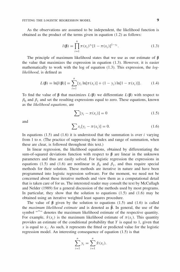
the value that maximizes the expression in equation (1.3). However, it is easiermathematically to work with the log of equation (1.3). This expression, the log-likelihood, is defined as
L(β) = ln[l(β)] =n∑
i=1
{yi ln[π(xi)] + (1 − yi) ln[1 − π(xi)]}. (1.4)
To find the value of β that maximizes L(β) we differentiate L(β) with respect toβ0 and β1 and set the resulting expressions equal to zero. These equations, knownas the likelihood equations, are∑
[yi − π(xi)] = 0 (1.5)
and ∑xi[yi − π(xi)] = 0. (1.6)
In equations (1.5) and (1.6) it is understood that the summation is over i varyingfrom 1 to n. (The practice of suppressing the index and range of summation, whenthese are clear, is followed throughout this text.)
In linear regression, the likelihood equations, obtained by differentiating thesum-of-squared deviations function with respect to β are linear in the unknownparameters and thus are easily solved. For logistic regression the expressions inequations (1.5) and (1.6) are nonlinear in β0 and β1, and thus require specialmethods for their solution. These methods are iterative in nature and have beenprogrammed into logistic regression software. For the moment, we need not beconcerned about these iterative methods and view them as a computational detailthat is taken care of for us. The interested reader may consult the text by McCullaghand Nelder (1989) for a general discussion of the methods used by most programs.In particular, they show that the solution to equations (1.5) and (1.6) may beobtained using an iterative weighted least squares procedure.
The value of β given by the solution to equations (1.5) and (1.6) is calledthe maximum likelihood estimate and is denoted as β. In general, the use of thesymbol “” denotes the maximum likelihood estimate of the respective quantity.For example, π(xi) is the maximum likelihood estimate of π(xi). This quantityprovides an estimate of the conditional probability that Y is equal to 1, given thatx is equal to xi . As such, it represents the fitted or predicted value for the logisticregression model. An interesting consequence of equation (1.5) is that
n∑i=1
yi =n∑
i=1
π(xi).
10 introduction to the logistic regression model
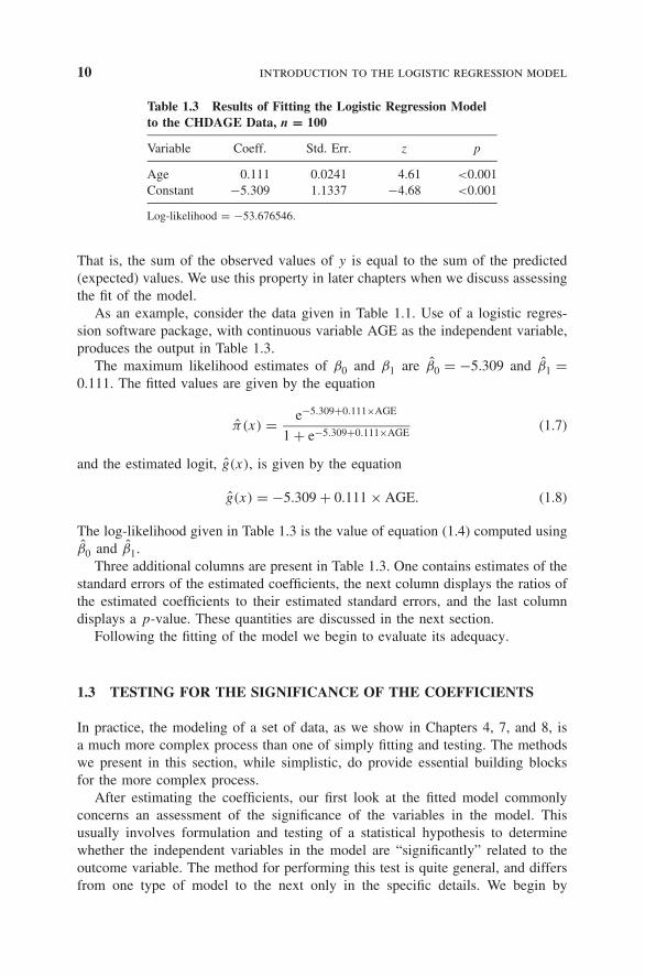
Table 1.3 Results of Fitting the Logistic Regression Modelto the CHDAGE Data, n = 100
Variable Coeff. Std. Err. z p
Age 0.111 0.0241 4.61 <0.001Constant −5.309 1.1337 −4.68 <0.001
Log-likelihood = −53.676546.
That is, the sum of the observed values of y is equal to the sum of the predicted(expected) values. We use this property in later chapters when we discuss assessingthe fit of the model.
As an example, consider the data given in Table 1.1. Use of a logistic regres-sion software package, with continuous variable AGE as the independent variable,produces the output in Table 1.3.
The maximum likelihood estimates of β0 and β1 are β0 = −5.309 and β1 =0.111. The fitted values are given by the equation
π(x) = e−5.309+0.111×AGE
1 + e−5.309+0.111×AGE(1.7)
and the estimated logit, g(x), is given by the equation
g(x) = −5.309 + 0.111 × AGE. (1.8)
The log-likelihood given in Table 1.3 is the value of equation (1.4) computed usingβ0 and β1.
Three additional columns are present in Table 1.3. One contains estimates of thestandard errors of the estimated coefficients, the next column displays the ratios ofthe estimated coefficients to their estimated standard errors, and the last columndisplays a p-value. These quantities are discussed in the next section.
Following the fitting of the model we begin to evaluate its adequacy.
1.3 TESTING FOR THE SIGNIFICANCE OF THE COEFFICIENTS
In practice, the modeling of a set of data, as we show in Chapters 4, 7, and 8, isa much more complex process than one of simply fitting and testing. The methodswe present in this section, while simplistic, do provide essential building blocksfor the more complex process.
After estimating the coefficients, our first look at the fitted model commonlyconcerns an assessment of the significance of the variables in the model. Thisusually involves formulation and testing of a statistical hypothesis to determinewhether the independent variables in the model are “significantly” related to theoutcome variable. The method for performing this test is quite general, and differsfrom one type of model to the next only in the specific details. We begin by
testing for the significance of the coefficients 11
discussing the general approach for a single independent variable. The multivariablecase is considered in Chapter 2.
One approach to testing for the significance of the coefficient of a variable inany model relates to the following question. Does the model that includes the vari-able in question tell us more about the outcome (or response) variable than a modelthat does not include that variable? This question is answered by comparing theobserved values of the response variable to those predicted by each of two models;the first with, and the second without, the variable in question. The mathematicalfunction used to compare the observed and predicted values depends on the partic-ular problem. If the predicted values with the variable in the model are better, ormore accurate in some sense, than when the variable is not in the model, then wefeel that the variable in question is “significant”. It is important to note that we arenot considering the question of whether the predicted values are an accurate rep-resentation of the observed values in an absolute sense (this is called goodness offit). Instead, our question is posed in a relative sense. The assessment of goodnessof fit is a more complex question that is discussed in detail in Chapter 5.
The general method for assessing significance of variables is easily illustratedin the linear regression model, and its use there motivates the approach used forlogistic regression. A comparison of the two approaches highlights the differencesbetween modeling continuous and dichotomous response variables.
In linear regression, one assesses the significance of the slope coefficient byforming what is referred to as an analysis of variance table. This table partitionsthe total sum-of-squared deviations of observations about their mean into two parts:(1) the sum-of-squared deviations of observations about the regression line SSE(or residual sum-of-squares) and (2) the sum-of-squares of predicted values, basedon the regression model, about the mean of the dependent variable SSR (or dueregression sum-of-squares). This is just a convenient way of displaying the com-parison of observed to predicted values under two models. In linear regression, thecomparison of observed and predicted values is based on the square of the distancebetween the two. If yi denotes the observed value and yi denotes the predictedvalue for the ith individual under the model, then the statistic used to evaluate thiscomparison is
SSE =n∑
i=1
(yi − yi )2.
Under the model not containing the independent variable in question the onlyparameter is β0, and β0 = y, the mean of the response variable. In this case, yi = y
and SSE is equal to the total sum-of-squares. When we include the independentvariable in the model, any decrease in SSE is due to the fact that the slope coefficientfor the independent variable is not zero. The change in the value of SSE is due tothe regression source of variability, denoted SSR. That is,
SSR =[
n∑i=1
(yi − yi
)2
]−
[n∑
i=1
(yi − yi
)2
].
12 introduction to the logistic regression model
In linear regression, interest focuses on the size of SSR. A large value suggeststhat the independent variable is important, whereas a small value suggests that theindependent variable is not helpful in predicting the response.
The guiding principle with logistic regression is the same: compare observedvalues of the response variable to predicted values obtained from models, with andwithout the variable in question. In logistic regression, comparison of observed topredicted values is based on the log-likelihood function defined in equation (1.4).To better understand this comparison, it is helpful conceptually to think of anobserved value of the response variable as also being a predicted value resultingfrom a saturated model. A saturated model is one that contains as many parametersas there are data points. (A simple example of a saturated model is fitting a linearregression model when there are only two data points, n = 2.)
The comparison of observed to predicted values using the likelihood function isbased on the following expression:
D = −2 ln
[(likelihood of the fitted model)
(likelihood of the saturated model)
]. (1.9)
The quantity inside the large brackets in the expression above is called the likelihoodratio. Using minus twice its log is necessary to obtain a quantity whose distributionis known and can therefore be used for hypothesis testing purposes. Such a test iscalled the likelihood ratio test. Using equation (1.4), equation (1.9) becomes
D = −2n∑
i=1
[yi ln
(πi
yi
)+ (1 − yi) ln
(1 − πi
1 − yi
)], (1.10)
where πi = π(xi).The statistic, D, in equation (1.10) is called the deviance, and for logistic
regression, it plays the same role that the residual sum-of-squares plays in lin-ear regression. In fact, the deviance as shown in equation (1.10), when computedfor linear regression, is identically equal to the SSE.
Furthermore, in a setting as shown in Table 1.1, where the values of the outcomevariable are either 0 or 1, the likelihood of the saturated model is identically equalto 1.0. Specifically, it follows from the definition of a saturated model that πi = yi
and the likelihood is
l(saturated model) =n∏
i=1
yyi
i × (1 − yi)(1−yi ) = 1.0.
Thus it follows from equation (1.9) that the deviance is
D = −2 ln(likelihood of the fitted model). (1.11)
Some software packages report the value of the deviance in equation (1.11) ratherthan the log-likelihood for the fitted model. In the context of testing for the signif-icance of a fitted model, we want to emphasize that we think of the deviance inthe same way that we think of the residual sum-of-squares in linear regression.
testing for the significance of the coefficients 13
In particular, to assess the significance of an independent variable we comparethe value of D with and without the independent variable in the equation. Thechange in D due to the inclusion of the independent variable in the model is:
G = D(model without the variable) − D(model with the variable).
This statistic, G, plays the same role in logistic regression that the numerator ofthe partial F -test does in linear regression. Because the likelihood of the satu-rated model is always common to both values of D being differenced, G can beexpressed as
G = −2 ln
[(likelihood without the variable)
(likelihood with the variable)
]. (1.12)
For the specific case of a single independent variable, it is easy to show thatwhen the variable is not in the model, the maximum likelihood estimate of β0 isln(n1/n0) where n1 = ∑
yi and n0 = ∑(1 − yi) and the predicted probability for
all subjects is constant, and equal to n1/n. In this setting, the value of G is:
G = −2 ln
⎡⎢⎢⎢⎢⎣(n1
n
)n1(n0
n
)n0
n∏i=1
πyi
i (1 − πi)(1−yi )
⎤⎥⎥⎥⎥⎦ , (1.13)
or
G = 2
{n∑
i=1
[yi ln
(πi
) + (1 − yi) ln(1 − πi)]
− [n1 ln
(n1
) + n0 ln(n0) − n ln(n)]}
. (1.14)
Under the hypothesis that β1 is equal to zero, the statistic G follows a chi-squaredistribution with 1 degree of freedom. Additional mathematical assumptions areneeded; however, for the above case they are rather nonrestrictive, and involvehaving a sufficiently large sample size, n, and enough subjects with both y = 0and y = 1. We discuss in later chapters that, as far as sample size is concerned,the key determinant is min(n0, n1).
As an example, we consider the model fit to the data in Table 1.1, whoseestimated coefficients and log-likelihood are given in Table 1.3. For these data thesample size is sufficiently large as n1 = 43 and n0 = 57. Evaluating G as shownin equation (1.14) yields
G = 2{−53.677 − [43 ln(43) + 57 ln(57) − 100 ln(100)]}= 2[−53.677 − (−68.331)] = 29.31.
14 introduction to the logistic regression model
The first term in this expression is the log-likelihood from the model contain-ing age (see Table 1.3), and the remainder of the expression simply substitutesn1 and n0 into the second part of equation (1.14). We use the symbol χ2(ν) todenote a chi-square random variable with ν degrees of freedom. Using this nota-tion, the p-value associated with this test is P [χ2(1) > 29.31] < 0.001; thus, wehave convincing evidence that AGE is a significant variable in predicting CHD.This is merely a statement of the statistical evidence for this variable. Other impor-tant factors to consider before concluding that the variable is clinically importantwould include the appropriateness of the fitted model, as well as inclusion of otherpotentially important variables.
As all logistic regression software report either the value of the log-likelihoodor the value of D, it is easy to check for the significance of the addition of newterms to the model or to verify a reported value of G. In the simple case of asingle independent variable, we first fit a model containing only the constant term.Next, we fit a model containing the independent variable along with the constant.This gives rise to another log-likelihood. The likelihood ratio test is obtained bymultiplying the difference between these two values by −2.
In the current example, the log-likelihood for the model containing only a con-stant term is −68.331. Fitting a model containing the independent variable (AGE)along with the constant term results in the log-likelihood shown in Table 1.3 of−53.677. Multiplying the difference in these log-likelihoods by −2 gives
−2 × [−68.331 − (−53.677)] = −2 × (−14.655) = 29.31.
This result, along with the associated p-value for the chi-square distribution, iscommonly reported in logistic regression software packages.
There are two other statistically equivalent tests: the Wald test and the Score test.The assumptions needed for each of these is the same as those of the likelihoodratio test in equation (1.14). A more complete discussion of these three tests andtheir assumptions may be found in Rao (1973).
The Wald test is equal to the ratio of the maximum likelihood estimate of theslope parameter, β1, to an estimate of its standard error. Under the null hypothesisand the sample size assumptions, this ratio follows a standard normal distribution.While we have not yet formally discussed how the estimates of the standard errorsof the estimated parameters are obtained, they are routinely printed out by computersoftware. For example, the Wald test for the coefficient for AGE in Table 1.3 isprovided in the column headed z and is
W = β1
SE(β1)= 0.111
0.024= 4.61.
The two-tailed p-value, provided in the last column of Table 1.3, is P(|z| > 4.61) <
0.001, where z denotes a random variable following the standard normal distribu-tion. Some software packages display the statistic W 2 = z2, which is distributedas chi-square with 1 degree of freedom. Hauck and Donner (1977) examined theperformance of the Wald test and found that it behaved in an aberrant manner, oftenfailing to reject the null hypothesis when the coefficient was significant using the
confidence interval estimation 15
likelihood ratio test. Thus, they recommended (and we agree) that the likelihoodratio test is preferred. We note that while the assertions of Hauk and Donner aretrue, we have never seen huge differences in the values of G and W 2. In prac-tice, the more troubling situation is when the values are close, and one test hasp < 0.05 and the other has p > 0.05. When this occurs, we use the p-value fromthe likelihood ratio test.
A test for the significance of a variable that does not require computing theestimate of the coefficient is the score test. Proponents of the score test cite thisreduced computational effort as its major advantage. Use of the test is limited bythe fact that it is not available in many software packages. The score test is basedon the distribution theory of the derivatives of the log-likelihood. In general, thisis a multivariate test requiring matrix calculations that are discussed in Chapter 2.
In the univariate case, this test is based on the conditional distribution ofthe derivative in equation (1.6), given the derivative in equation (1.5). In thiscase, we can write down an expression for the Score test. The test uses thevalue of equation (1.6) computed using β0 = ln(n1/n0) and β1 = 0. As notedearlier, under these parameter values, π = n1/n = y and the left-hand side ofequation (1.6) becomes
∑xi(yi − y). It may be shown that the estimated variance
is y(1 − y)∑
(xi − x)2. The test statistic for the score test (ST) is
ST =
n∑i=1
xi(yi − y)√√√√y(1 − y)
n∑i=1
(xi − x)2
.
As an example of the score test, consider the model fit to the data in Table 1.1.The value of the test statistic for this example is
ST = 296.66√3333.742
= 5.14
and the two tailed p-value is P(|z| > 5.14) < 0.001. We note that, for this example,the values of the three test statistics are nearly the same (note:
√G = 5.41).
In summary, the method for testing the significance of the coefficient of avariable in logistic regression is similar to the approach used in linear regression;however, it is based on the likelihood function for a dichotomous outcome variableunder the logistic regression model.
1.4 CONFIDENCE INTERVAL ESTIMATION
An important adjunct to testing for significance of the model, discussed inSection 1.3, is calculation and interpretation of confidence intervals for parametersof interest. As is the case in linear regression we can obtain these for the slope,intercept and the “line” (i.e., the logit). In some settings it may be of interest toprovide interval estimates for the fitted values (i.e., the predicted probabilities).
16 introduction to the logistic regression model
The basis for construction of the interval estimators is the same statistical theorywe used to formulate the tests for significance of the model. In particular, the confi-dence interval estimators for the slope and intercept are, most often, based on theirrespective Wald tests and are sometimes referred to as Wald-based confidence inter-vals. The endpoints of a 100(1 − α)% confidence interval for the slope coefficientare
β1 ± z1−α/2SE(β1) (1.15)
and for the intercept they are
β0 ± z1−α/2SE(β0) (1.16)
where z1−α/2 is the upper 100(1 − α/2)% point from the standard normal dis-tribution and SE(·) denotes a model-based estimator of the standard error of therespective parameter estimator. We defer discussion of the actual formula used forcalculating the estimators of the standard errors to Chapter 2. For the moment, weuse the fact that estimated values are provided in the output following the fit of amodel and, in addition, many packages also provide the endpoints of the intervalestimates.
As an example, consider the model fit to the data in Table 1.1 regressingAGE on the presence or absence of CHD. The results are presented in Table 1.3.The endpoints of a 95 percent confidence interval for the slope coefficient fromequation (1.15) are 0.111 ± 1.96 × 0.0241, yielding the interval (0.064, 0.158). Wedefer a detailed discussion of the interpretation of these results to Chapter 3. Briefly,the results suggest that the change in the log-odds of CHD per one year increasein age is 0.111 and the change could be as little as 0.064 or as much as 0.158 with95 percent confidence.
As is the case with any regression model, the constant term provides an estimateof the response at x = 0 unless the independent variable has been centered at someclinically meaningful value. In our example, the constant provides an estimate ofthe log-odds ratio of CHD at zero years of age. As a result, the constant term, byitself, has no useful clinical interpretation. In any event, from equation (1.16), theendpoints of a 95 percent confidence interval for the constant are −5.309 ± 1.96 ×1.1337, yielding the interval (−7.531,−3.087).
The logit is the linear part of the logistic regression model and, as such, is mostsimilar to the fitted line in a linear regression model. The estimator of the logit is
g(x) = β0 + β1x. (1.17)
The estimator of the variance of the estimator of the logit requires obtaining thevariance of a sum. In this case it is
Var[g(x)] = Var(β0) + x2Var(β1) + 2xCov(β0, β1). (1.18)
In general, the variance of a sum is equal to the sum of the variance of eachterm and twice the covariance of each possible pair of terms formed from the
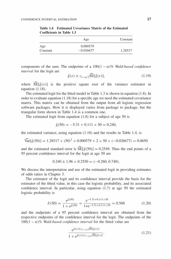
confidence interval estimation 17
Table 1.4 Estimated Covariance Matrix of the EstimatedCoefficients in Table 1.3
Age Constant
Age 0.000579Constant −0.026677 1.28517
components of the sum. The endpoints of a 100(1 − α)% Wald-based confidenceinterval for the logit are
g(x) ± z1−α/2SE[g(x)], (1.19)
where SE[g(x)] is the positive square root of the variance estimator inequation (1.18).
The estimated logit for the fitted model in Table 1.3 is shown in equation (1.8). Inorder to evaluate equation (1.18) for a specific age we need the estimated covariancematrix. This matrix can be obtained from the output from all logistic regressionsoftware packages. How it is displayed varies from package to package, but thetriangular form shown in Table 1.4 is a common one.
The estimated logit from equation (1.8) for a subject of age 50 is
g(50) = −5.31 + 0.111 × 50 = 0.240,
the estimated variance, using equation (1.18) and the results in Table 1.4, is
Var[g(50)] = 1.28517 + (50)2 × 0.000579 + 2 × 50 × (−0.026677) = 0.0650
and the estimated standard error is SE[g(50)] = 0.2549. Thus the end points of a95 percent confidence interval for the logit at age 50 are
0.240 ± 1.96 × 0.2550 = (−0.260, 0.740).
We discuss the interpretation and use of the estimated logit in providing estimatesof odds ratios in Chapter 3.
The estimator of the logit and its confidence interval provide the basis for theestimator of the fitted value, in this case the logistic probability, and its associatedconfidence interval. In particular, using equation (1.7) at age 50 the estimatedlogistic probability is
π(50) = eg(50)
1 + eg(50)= e−5.31+0.111×50
1+e−5.31+0.111×50= 0.560 (1.20)
and the endpoints of a 95 percent confidence interval are obtained from therespective endpoints of the confidence interval for the logit. The endpoints of the100(1 − α)% Wald-based confidence interval for the fitted value are
eg(x)±z1−α/2SE[g(x)]
1 + eg(x)±z1−α/2SE[g(x)]. (1.21)
18 introduction to the logistic regression model
Using the example at age 50 to demonstrate the calculations, the lower limit is
e−0.260
1 + e−0.260= 0.435,
and the upper limit ise0.740
1 + e0.740= 0.677.
We have found that a major mistake often made by data analysts new to logis-tic regression modeling is to try and apply estimates on the probability scale toindividual subjects. The fitted value computed in equation (1.20) is analogous to aparticular point on the line obtained from a linear regression. In linear regressioneach point on the fitted line provides an estimate of the mean of the dependentvariable in a population of subjects with covariate value “x”. Thus the value of0.56 in equation (1.20) is an estimate of the mean (i.e., proportion) of 50-year-oldsubjects in the population sampled that have evidence of CHD. An individual 50-year-old subject either does or does not have evidence of CHD. The confidenceinterval suggests that this mean could be between 0.435 and 0.677 with 95 percentconfidence. We discuss the use and interpretation of fitted values in greater detailin Chapter 3.
One application of fitted logistic regression models that has received a lot ofattention in the subject matter literature is using model-based fitted values similarto the one in equation (1.20) to predict the value of a binary dependent value inindividual subjects. This process is called classification and has a long history instatistics where it is referred to as discriminant analysis. We discuss the classifica-tion problem in detail in Chapter 4. We also discuss discriminant analysis withinthe context of a method for obtaining estimators of the coefficients in the nextsection.
The coverage∗† of the Wald-based confidence interval estimators inequations (1.15) and (1.16) depends on the assumption that the distribution of themaximum likelihood estimators is normal. Potential sensitivity to this assumptionis the main reason that the likelihood ratio test is recommended over the Wald testfor assessing the significance of individual coefficients, as well as for the overallmodel. In settings where the number of events (y = 1) and/or the sample sizeis small the normality assumption is suspect and a log-likelihood function-basedconfidence interval can have better coverage. Until recently routines to computethese intervals were not available in most software packages. Cox and Snell(1989, p. 179–183) discuss the theory behind likelihood intervals, and Venzonand Moolgavkar (1988) describe an efficient way to calculate the end points.
∗The remainder of this section is more advanced material that can be skipped on first reading of thetext.†The term coverage of an interval estimator refers to the percent of time confidence intervals computedin a similar manner contain the true parameter value. Research has shown that when the normalityassumption does not hold, Wald-based confidence intervals can be too narrow and thus contain the trueparameter with a smaller percentage than the stated confidence coefficient.
confidence interval estimation 19
Royston (2007) describes a STATA [StataCorp (2011)] routine that implementsthe Venzon and Moolgavkar method that we use for the examples in this text. TheSAS package’s logistic regression procedure [SAS Institute Inc. (2009)] has theoption to obtain likelihood confidence intervals.
The likelihood-based confidence interval estimator for a coefficient can be con-cisely described as the interval of values, β∗, for which the likelihood ratio testwould fail to reject the hypothesis, Ho : β = β∗, at the stated 1 − α percent signif-icance level. The two end points, βlower and βupper, of this interval for a coefficientare defined as follows:
2[l(β) − lp(βupper)] = 2[l(β) − lp(βlower)] = χ21−α(1), (1.22)
where l(β) is the value of the log-likelihood of the fitted model and lp(β) is thevalue of the profile log-likelihood. A value of the profile log-likelihood is computedby first specifying/fixing a value for the coefficient of interest, for example the slopecoefficient for age, and then finding the value of the intercept coefficient, using theVenzon and Moolgavkar method, that maximizes the log-likelihood. This processis repeated over a grid of values of the specified coefficient, for example, values ofβ∗, until the solutions to equation (1.22) are found. The results can be presentedgraphically or in standard interval form. We illustrate both in the example below.
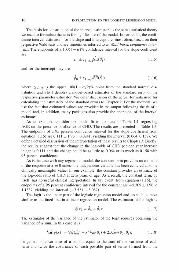
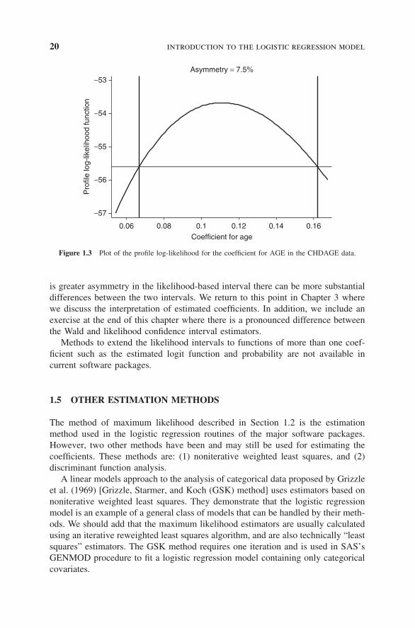
As an example, we show in Figure 1.3 a plot of the profile log-likelihood for thecoefficient for AGE using the CHDAGE data in Table 1.1. The end points of the95 percent likelihood interval are βlower = 0.067 and βupper = 0.162 and are shownin the figure where the two vertical lines intersect the “x” axis. The horizontal linein the figure is drawn at the value
−55.5964 = −53.6756 −(
3.8416
2
),
where −53.6756 is the value of the log-likelihood of the fitted model from Table 1.3and 3.8416 is the 95th percentile of the chi-square distribution with 1 degree offreedom.
The quantity “Asymmetry” in Figure 1.3 is a measure of asymmetry of theprofile log-likelihood that is the difference between the lengths of the upper partof the interval, βupper − β, to the lower part, β − βlower, as a percent of the totallength, βupper − βlower. In the example the value is
A = 100 × (0.162 − 0.111) − (0.111 − 0.067)
(0.162 − 0.067)∼= 7.5%.
As the upper and lower endpoints of the Wald-based confidence interval inequation (1.15) are equidistant from the maximum likelihood estimator, it hasasymmetry A = 0.
In this example, the Wald-based confidence interval for the coefficient for ageis (0.064, 0.158). The likelihood interval is (0.067, 0.162), which is only 1.1%wider than the Wald-based interval. So there is not a great deal of pure numericdifference in the two intervals and the asymmetry is small. In settings where there
20 introduction to the logistic regression model
−57
−56
−55
−54
−53P
rofil
e lo
g-lik
elih
ood
func
tion
0.06 0.08 0.1 0.12 0.14 0.16
Coefficient for age
Asymmetry = 7.5%
Figure 1.3 Plot of the profile log-likelihood for the coefficient for AGE in the CHDAGE data.
is greater asymmetry in the likelihood-based interval there can be more substantialdifferences between the two intervals. We return to this point in Chapter 3 wherewe discuss the interpretation of estimated coefficients. In addition, we include anexercise at the end of this chapter where there is a pronounced difference betweenthe Wald and likelihood confidence interval estimators.
Methods to extend the likelihood intervals to functions of more than one coef-ficient such as the estimated logit function and probability are not available incurrent software packages.
1.5 OTHER ESTIMATION METHODS
The method of maximum likelihood described in Section 1.2 is the estimationmethod used in the logistic regression routines of the major software packages.However, two other methods have been and may still be used for estimating thecoefficients. These methods are: (1) noniterative weighted least squares, and (2)discriminant function analysis.
A linear models approach to the analysis of categorical data proposed by Grizzleet al. (1969) [Grizzle, Starmer, and Koch (GSK) method] uses estimators based onnoniterative weighted least squares. They demonstrate that the logistic regressionmodel is an example of a general class of models that can be handled by their meth-ods. We should add that the maximum likelihood estimators are usually calculatedusing an iterative reweighted least squares algorithm, and are also technically “leastsquares” estimators. The GSK method requires one iteration and is used in SAS’sGENMOD procedure to fit a logistic regression model containing only categoricalcovariates.
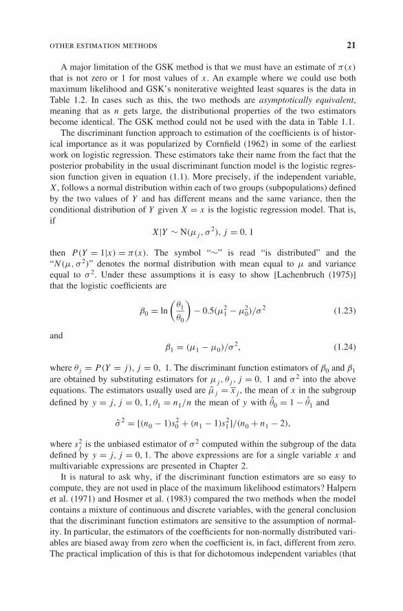
other estimation methods 21
A major limitation of the GSK method is that we must have an estimate of π(x)
that is not zero or 1 for most values of x. An example where we could use bothmaximum likelihood and GSK’s noniterative weighted least squares is the data inTable 1.2. In cases such as this, the two methods are asymptotically equivalent,meaning that as n gets large, the distributional properties of the two estimatorsbecome identical. The GSK method could not be used with the data in Table 1.1.
The discriminant function approach to estimation of the coefficients is of histor-ical importance as it was popularized by Cornfield (1962) in some of the earliestwork on logistic regression. These estimators take their name from the fact that theposterior probability in the usual discriminant function model is the logistic regres-sion function given in equation (1.1). More precisely, if the independent variable,X, follows a normal distribution within each of two groups (subpopulations) definedby the two values of Y and has different means and the same variance, then theconditional distribution of Y given X = x is the logistic regression model. That is,if
X|Y ∼ N(μj , σ2), j = 0, 1
then P(Y = 1|x) = π(x). The symbol “∼” is read “is distributed” and the“N(μ, σ 2)” denotes the normal distribution with mean equal to μ and varianceequal to σ 2. Under these assumptions it is easy to show [Lachenbruch (1975)]that the logistic coefficients are
β0 = ln
(θ1
θ0
)− 0.5(μ2
1 − μ20)/σ
2 (1.23)
andβ1 = (μ1 − μ0)/σ
2, (1.24)
where θj = P(Y = j), j = 0, 1. The discriminant function estimators of β0 and β1are obtained by substituting estimators for μj , θj , j = 0, 1 and σ 2 into the aboveequations. The estimators usually used are μj = xj , the mean of x in the subgroupdefined by y = j, j = 0, 1, θ1 = n1/n the mean of y with θ0 = 1 − θ1 and
σ 2 = [(n0 − 1)s20 + (n1 − 1)s2
1 ]/(n0 + n1 − 2),
where s2j is the unbiased estimator of σ 2 computed within the subgroup of the data
defined by y = j, j = 0, 1. The above expressions are for a single variable x andmultivariable expressions are presented in Chapter 2.
It is natural to ask why, if the discriminant function estimators are so easy tocompute, they are not used in place of the maximum likelihood estimators? Halpernet al. (1971) and Hosmer et al. (1983) compared the two methods when the modelcontains a mixture of continuous and discrete variables, with the general conclusionthat the discriminant function estimators are sensitive to the assumption of normal-ity. In particular, the estimators of the coefficients for non-normally distributed vari-ables are biased away from zero when the coefficient is, in fact, different from zero.The practical implication of this is that for dichotomous independent variables (that
22 introduction to the logistic regression model
occur in many situations), the discriminant function estimators overestimate themagnitude of the coefficient. Lyles et al. (2009) describe a clever linear regression-based approach to compute the discriminant function estimator of the coefficientfor a single continuous variable that, when their assumptions of normality hold,has better statistical properties than the maximum likelihood estimator. We discusstheir multivariable extension and some of its practical limitations in Chapter 2.
At this point it may be helpful to delineate more carefully the various usesof the term maximum likelihood, as it applies to the estimation of the logisticregression coefficients. Under the assumptions of the discriminant function modelstated above, the estimators obtained from equations (1.23) and (1.24) are maximumlikelihood estimators. The estimators obtained from equations (1.5) and (1.6) arebased on the conditional distribution of Y given X and, as such, are technically“conditional maximum likelihood estimators”. It is common practice to drop theword “conditional” when describing the estimators given in equations (1.5) and(1.6). In this text, we use the word conditional to describe estimators in logisticregression with matched data as discussed in Chapter 7.
In summary there are alternative methods of estimation for some data configu-rations that are computationally quicker; however, we use the maximum likelihoodmethod described in Section 1.2 throughout the rest of this text.
1.6 DATA SETS USED IN EXAMPLES AND EXERCISES
A number of different data sets are used in the examples as well as the exercisesfor the purpose of demonstrating various aspects of logistic regression modeling.Six of the data sets used throughout the text are described below. Other data setsare introduced as needed in later chapters. Some of the data sets were used inthe previous editions of this text, for example the ICU and Low Birth Weightdata, while others are new to this edition. All data sets used in this text may beobtained from links to web sites at John Wiley & Sons Inc. and the University ofMassachusetts given in the Preface.
1.6.1 The ICU Study
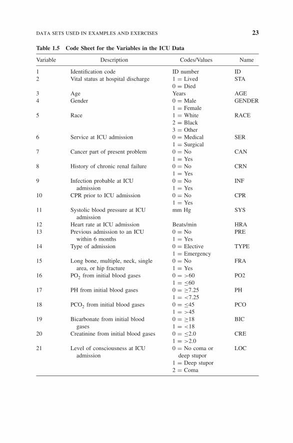
The ICU study data set consists of a sample of 200 subjects who were part of amuch larger study on survival of patients following admission to an adult intensivecare unit (ICU). The major goal of this study was to develop a logistic regressionmodel to predict the probability of survival to hospital discharge of these patients.A number of publications have appeared that have focused on various facets ofthis problem. The reader wishing to learn more about the clinical aspects of thisstudy should start with Lemeshow et al. (1988). For a more up-to-date discussionof modeling the outcome of ICU patients the reader is referred to Lemeshow andLe Gall (1994) and to Lemeshow et al. (1993). The actual observed variable valueshave been modified to protect subject confidentiality. A code sheet for the variablesto be considered in this text is given in Table 1.5. We refer to this data set as theICU data.
data sets used in examples and exercises 23
Table 1.5 Code Sheet for the Variables in the ICU Data
Variable Description Codes/Values Name
1 Identification code ID number ID2 Vital status at hospital discharge 1 = Lived
0 = DiedSTA
3 Age Years AGE4 Gender 0 = Male
1 = FemaleGENDER
5 Race 1 = White2 = Black3 = Other
RACE
6 Service at ICU admission 0 = Medical1 = Surgical
SER
7 Cancer part of present problem 0 = No1 = Yes
CAN
8 History of chronic renal failure 0 = No1 = Yes
CRN
9 Infection probable at ICUadmission
0 = No1 = Yes
INF
10 CPR prior to ICU admission 0 = No1 = Yes
CPR
11 Systolic blood pressure at ICUadmission
mm Hg SYS
12 Heart rate at ICU admission Beats/min HRA13 Previous admission to an ICU
within 6 months0 = No1 = Yes
PRE
14 Type of admission 0 = Elective1 = Emergency
TYPE
15 Long bone, multiple, neck, singlearea, or hip fracture
0 = No1 = Yes
FRA
16 PO2 from initial blood gases 0 = >601 = ≤60
PO2
17 PH from initial blood gases 0 = ≥7.251 = <7.25
PH
18 PCO2 from initial blood gases 0 = ≤451 = >45
PCO
19 Bicarbonate from initial bloodgases
0 = ≥181 = <18
BIC
20 Creatinine from initial blood gases 0 = ≤2.01 = >2.0
CRE
21 Level of consciousness at ICUadmission
0 = No coma ordeep stupor
1 = Deep stupor2 = Coma
LOC
24 introduction to the logistic regression model
Table 1.6 Code Sheet for the Variables in the Low Birth Weight Data
Variable Description Codes/Values Name
1 Identification code 1–189 ID2 Low birth weight 0 = ≥2500 g
1 = <2500 gLOW
3 Age of mother Years AGE4 Weight of mother at last menstrual period Pounds LWT5 Race 1 = White
2 = Black3 = Other
RACE
6 Smoking status during pregnancy 0 = No1 = Yes
SMOKE
7 History of premature labor 0 = None1 = One2 = Two, etc.
PTL
8 History of hypertension 0 = No1 = Yes
HT
9 Presence of uterine irritability 0 = No1 = Yes
UI
10 Number of physician visits during the firsttrimester
0 = None1 = One2 = Two, etc.
FTV
11 Recorded birth weight Grams BWT
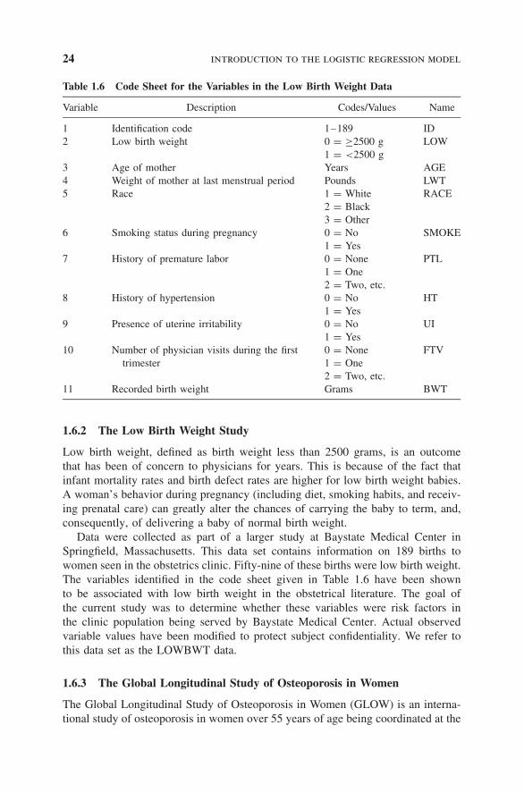
1.6.2 The Low Birth Weight Study
Low birth weight, defined as birth weight less than 2500 grams, is an outcomethat has been of concern to physicians for years. This is because of the fact thatinfant mortality rates and birth defect rates are higher for low birth weight babies.A woman’s behavior during pregnancy (including diet, smoking habits, and receiv-ing prenatal care) can greatly alter the chances of carrying the baby to term, and,consequently, of delivering a baby of normal birth weight.
Data were collected as part of a larger study at Baystate Medical Center inSpringfield, Massachusetts. This data set contains information on 189 births towomen seen in the obstetrics clinic. Fifty-nine of these births were low birth weight.The variables identified in the code sheet given in Table 1.6 have been shownto be associated with low birth weight in the obstetrical literature. The goal ofthe current study was to determine whether these variables were risk factors inthe clinic population being served by Baystate Medical Center. Actual observedvariable values have been modified to protect subject confidentiality. We refer tothis data set as the LOWBWT data.
1.6.3 The Global Longitudinal Study of Osteoporosis in Women
The Global Longitudinal Study of Osteoporosis in Women (GLOW) is an interna-tional study of osteoporosis in women over 55 years of age being coordinated at the
data sets used in examples and exercises 25
Table 1.7 Code Sheet for Variables in the GLOW Study
Variable Description Codes/Values Name
1 Identification code 1–n SUB_ID2 Study site 1–6 SITE_ID3 Physician ID code 128 unique codes PHY_ID4 History of prior fracture 1 = Yes
0 = NoPRIORFRAC
5 Age at enrollment Years AGE6 Weight at enrollment Kilograms WEIGHT7 Height at enrollment Centimeters HEIGHT8 Body mass index kg/m2 BMI9 Menopause before age 45 1 = Yes
0 = NoPREMENO
10 Mother had hip fracture 1 = Yes0 = No
MOMFRAC
11 Arms are needed to stand froma chair
1 = Yes0 = No
ARMASSIST
12 Former or current smoker 1 = Yes0 = No
SMOKE
13 Self-reported risk of fracture 1 = Less than others of thesame age
2 = Same as others of the sameage
3 = Greater than others of thesame age
RATERISK
14 Fracture risk score Composite risk scorea FRACSCORE15 Any fracture in first year 1 = Yes
0 = NoFRACTURE
aFRACSCORE = 0 × (AGE ≤ 60) + 1 × (60 < AGE ≤ 65) + 2 × (65 < AGE ≤ 70) + 3 × (70 <
AGE ≤ 75) + 4 × (75 < AGE ≤ 80) + 5 × (80 < AGE ≤ 85) + 6 × (AGE > 85) + (PRIORFRAC= 1) + (MOMFRAC = 1) + (WEIGHT < 56.8) + 2 × (ARMASSIST = 1) + (SMOKE = 1).
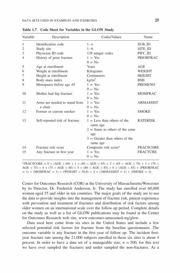
Center for Outcomes Research (COR) at the University of Massachusetts/Worcesterby its Director, Dr. Frederick Anderson, Jr. The study has enrolled over 60,000women aged 55 and older in ten countries. The major goals of the study are to usethe data to provide insights into the management of fracture risk, patient experiencewith prevention and treatment of fractures and distribution of risk factors amongolder women on an international scale over the follow up period. Complete detailson the study as well as a list of GLOW publications may be found at the Centerfor Outcomes Research web site, www.outcomes-umassmed.org/glow.
Data used here come from six sites in the United States and include a fewselected potential risk factors for fracture from the baseline questionnaire. Theoutcome variable is any fracture in the first year of follow up. The incident first-year fracture rate among the 21,000 subjects enrolled in these six sites is about 4percent. In order to have a data set of a manageable size, n = 500, for this textwe have over sampled the fractures and under sampled the non-fractures. As a
26 introduction to the logistic regression model
result associations and conclusions from modeling these data do not apply to thestudy cohort as a whole. Data have been modified to protect subject confidentiality.We thank Dr. Gordon Fitzgerald of COR for his help in obtaining these data sets.A code sheet for the variables is shown in Table 1.7. This data set is named theGLOW500 data.
1.6.4 The Adolescent Placement Study
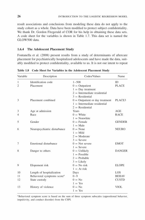
Fontanella et al. (2008) present results from a study of determinants of aftercareplacement for psychiatrically hospitalized adolescents and have made the data, suit-ably modified to protect confidentiality, available to us. It is not our intent to repeat
Table 1.8 Code Sheet for Variables in the Adolescent Placement Study
Variable Description Codes/Values Name
1 Identification code 1–508 ID2 Placement 0 = Outpatient
1 = Day treatment2 = Intermediate residential3 = Residential
PLACE
3 Placement combined 0 = Outpatient or day treatment1 = Intermediate residential2 = Residential
PLACE3
3 Age at admission Years AGE4 Race 0 = White
1 = NonwhiteRACE
5 Gender 0 = Female1 = Male
GENDER
6 Neuropsychiatric disturbance 0 = None1 = Mild2 = Moderate3 = Severe
NEURO
7 Emotional disturbance 0 = Not severe1 = Severe
EMOT
8 Danger to others 0 = Unlikely1 = Possible2 = Probable3 = Likely
DANGER
9 Elopement risk 0 = No risk1 = At risk
ELOPE
10 Length of hospitalization Days LOS11 Behavioral symptoms scorea 0–9 BEHAV12 State custody 0 = No
1 = YesCUSTD
13 History of violence 0 = No1 = Yes
VIOL
aBehavioral symptom score is based on the sum of three symptom subscales (oppositional behavior,impulsivity, and conduct disorder) from the CSPI.
data sets used in examples and exercises 27
the detailed analyses reported in their paper, but rather to use the data to motivateand describe methods for modeling a multinomial or ordinal scaled outcome usinglogistic regression models. As such, we selected a subset of variables, which aredescribed in Table 1.8. This data set is referred to as the APS data.
1.6.5 The Burn Injury Study
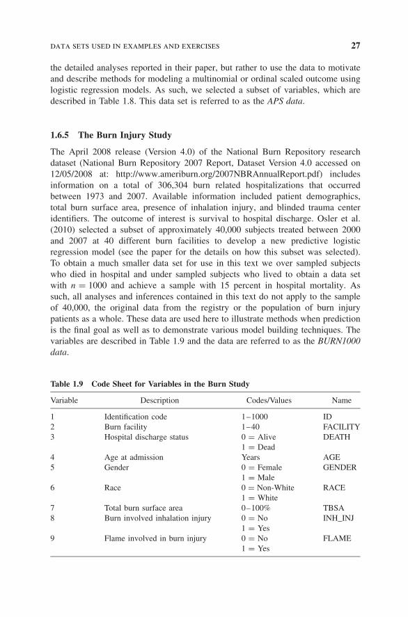
The April 2008 release (Version 4.0) of the National Burn Repository researchdataset (National Burn Repository 2007 Report, Dataset Version 4.0 accessed on12/05/2008 at: http://www.ameriburn.org/2007NBRAnnualReport.pdf) includesinformation on a total of 306,304 burn related hospitalizations that occurredbetween 1973 and 2007. Available information included patient demographics,total burn surface area, presence of inhalation injury, and blinded trauma centeridentifiers. The outcome of interest is survival to hospital discharge. Osler et al.(2010) selected a subset of approximately 40,000 subjects treated between 2000and 2007 at 40 different burn facilities to develop a new predictive logisticregression model (see the paper for the details on how this subset was selected).To obtain a much smaller data set for use in this text we over sampled subjectswho died in hospital and under sampled subjects who lived to obtain a data setwith n = 1000 and achieve a sample with 15 percent in hospital mortality. Assuch, all analyses and inferences contained in this text do not apply to the sampleof 40,000, the original data from the registry or the population of burn injurypatients as a whole. These data are used here to illustrate methods when predictionis the final goal as well as to demonstrate various model building techniques. Thevariables are described in Table 1.9 and the data are referred to as the BURN1000data.
Table 1.9 Code Sheet for Variables in the Burn Study
Variable Description Codes/Values Name
1 Identification code 1–1000 ID2 Burn facility 1–40 FACILITY3 Hospital discharge status 0 = Alive
1 = DeadDEATH
4 Age at admission Years AGE5 Gender 0 = Female
1 = MaleGENDER
6 Race 0 = Non-White1 = White
RACE
7 Total burn surface area 0–100% TBSA8 Burn involved inhalation injury 0 = No
1 = YesINH_INJ
9 Flame involved in burn injury 0 = No1 = Yes
FLAME

28 introduction to the logistic regression model
Table 1.10 Code Sheet for Variables in the Myopia Study
Variable Variable Description Values/Labels Variable Name
1 Subject identifier Integer (range 1–1503) ID2 Year subject entered the study Year STUDYYEAR3 Myopia within the first 5 yr of
follow upa
0 = No1 = Yes
MYOPIC
4 Age at first visit Years AGE5 Gender 0 = Male
1 = FemaleGENDER
6 Spherical equivalent refractionb Diopter SPHEQ7 Axial lengthc mm AL8 Anterior chamber depthd mm ACD9 Lens thicknesse mm LT10 Vitreous chamber depthf mm VCD11 How many hours per week
outside of school the childspent engaging insports/outdoor activities
Hours per week SPORTHR
12 How many hours per weekoutside of school the childspent reading for pleasure
Hours per week READHR
13 How many hours per weekoutside of school the childspent playing video/computergames or working on thecomputer
Hours per week COMPHR
14 How many hours per weekoutside of school the childspent reading or studying forschool assignments
Hours per week STUDYHR
15 How many hours per weekoutside of school the childspent watching television
Hours per week TVHR
16 Composite of near-workactivities
Hours per week DIOPTERHR
17 Was the subject’s mothermyopic?g
0 = No1 = Yes
MOMMY
18 Was the subject’s fathermyopic?
0 = No1 = Yes
DADMY
aMYOPIC is defined as SPHEQ <= −0.75D.bA measure of the eye’s effective focusing power. Eyes that are “normal” (don’t require glasses orcontact lenses) have spherical equivalents between −0.25 diopters (D) and +1.00 D. The more negativethe spherical equivalent, the more myopic the subject.cThe length of eye from front to back.dThe length from front to back of the aqueous-containing space of the eye between the cornea and theiris.eThe length from front to back of the crystalline lens.f The length from front to back of the aqueous-containing space of the eye in front of the retina.gDIOPTERHR = 3 × (READHR + STUDYHR) + 2 × COMPHR + TVHR.

data sets used in examples and exercises 29
Table 1.11 Variables in the Modified NHANES Data Set
Variable Description Code/values Name
1 Identification code 1–6482 ID2 Gender 0 = Male,
1 = FemaleGENDER
3 Age at screening Years AGE4 Marital status 1 = Married
2 = Widowed3 = Divorced4 = Separated5 = Never married6 = Living together
MARSTAT
5 Statistical weight 4084.478–153810.3 SAMPLEWT6 Pseudo-PSU 1, 2 PSU7 Pseudo-stratum 1–15 STRATA8 Total cholesterol mg/dl TCHOL9 HDL-cholesterol mg/dl HDL10 Systolic blood pressure mm Hg SYSBP11 Diastolic blood pressure mm Hg DBP12 Weight kg WT13 Standing height cm HT14 Body mass index kg/m2 BMI15 Vigorous work activity 0 = Yes,
1 = NoVIGWRK
16 Moderate work activity 0 = Yes,1 = No
MODWRK
17 Walk or bicycle 0 = Yes,1 = No
WLKBIK
18 Vigorous recreational activities 0 = Yes,1 = No
VIGRECEXR
19 Moderate recreational activities 0 = Yes,1 = No
MODRECEXR
20 Minutes of sedentary activityper week
Minutes SEDMIN
21 BMI > 35 0 = No,1 = Yes
OBESE
1.6.6 The Myopia Study
Myopia, more commonly referred to as nearsightedness, is an eye condition wherean individual has difficulty seeing things at a distance. This condition is primarilybecause the eyeball is too long. In an eye that sees normally, the image of what isbeing viewed is transmitted to the back portion of the eye, or retina, and hits theretina to form a clear picture. In the myopic eye, the image focuses in front of theretina, so the resultant image on the retina itself is blurry. The blurry image createsproblems with a variety of distance viewing tasks (e.g., reading the blackboard,

30 introduction to the logistic regression model
Table 1.12 Code Sheet for the Variables in the Polypharmacy Data Set
Variable Description Codes/Values Name
1 Subject ID ID number 1–500 ID2 Outcome; taking drugs from
more than three differentclasses
0 = Not taking drugsfrom more than threeclasses
1 = Taking drugs frommore than three classes
POLYPHARMACY
3 Number of outpatient mentalhealth visits (MHV)
0 = None1 = One to five2 = Six to fourteen3 = Greater than 14
MHV4
4 Number of inpatient mentalhealth visits (MHV)
0 = None1 = One2 = More than one
INPTMHV3
5 Year 2002–2008 YEAR6 Group 1 = Covered families and
children (CFC)2 = Aged, blind or
disabled (ABD)3 = Foster care (FOS)
GROUP
7 Location 0 = Urban1 = Rural
URBAN
8 Comorbidity 0 = No1 = Yes
COMORBID
9 Any primary diagnosis (bipolar,depression, etc.)
0 = No1 = Yes
ANYPRIM
10 Number of primary diagnosis 0 = None1 = One2 = More than one
NUMPRIMRC
11 Gender 0 = Female1 = Male
GENDER
12 Race 0 = White1 = Black2 = Other
RACE
13 Ethnic category 0 = NonHispanic1 = Hispanic
ETHNIC
14 Age Years and months (twodecimal places)
AGE
doing homework, driving, playing sports) and requires wearing glasses or contactlenses to correct the problem. Myopia onset is typically between the ages of 8 and12 years with cessation of the underlying eye growth that causes it by age 15–16years.
The risk factors for the development of myopia have been debated for a longtime and include genetic factors (e.g., family history of myopia) and the amount
data sets used in examples and exercises 31
and type of visual activity that a child performs (e.g., studying, reading, TV watch-ing, computer or video game playing, and sports/outdoor activity). There is strongevidence that having myopic parents increases the chance that a child will becomemyopic, and weaker evidence that certain types of visual activities (called nearwork, e.g., reading) increase the chance that a child will become myopic.
These data are a subset of data from the Orinda Longitudinal Study of Myopia(OLSM), a cohort study of ocular component development and risk factors forthe onset of myopia in children, which evolved into the Collaborative LongitudinalEvaluation of Ethnicity and Refractive Error (CLEERE) Study, and both OLSM andCLEERE were funded by the National Institutes of Health/National Eye Institute.OLSM was based at the University of California, Berkeley [see Zadnik et al. (1993,1994)]. Data collection began in the 1989–1990 school year and continued annuallythrough the 2000–2001 school year. All data about the parts that make up the eye(the ocular components) were collected during an examination during the schoolday. Data on family history and visual activities were collected yearly in a surveycompleted by a parent or guardian.
The dataset used in this text is from 618 of the subjects who had at least fiveyears of followup and were not myopic when they entered the study. All data arefrom their initial exam and includes 17 variables. In addition to the ocular datathere is information on age at entry, year of entry, family history of myopia andhours of various visual activities. The ocular data come from a subject’s right eye.A subject was coded as myopic if they became myopic at any time during the firstfive years of followup. We refer to this data set, in Table 1.10, as the MYOPIA data.
1.6.7 The NHANES Study
The National Health and Nutrition Examination Survey (NHANES), a major effortof the National Center for Health Statistics, was conceived in the early 1960s toprovide nationally representative and reliable data on the health and nutritionalstatus of adults and children in the United States. NHANES has since evolvedinto a ongoing survey program that provides the best available national estimatesof the prevalence of, and risk factors for, targeted diseases in the United Statespopulation. The survey collects interview and physical exam data on a nationallyrepresentative, multistage probability sample of about 5,000 persons each year, whoare chosen to be representative of the civilian, non-institutionalized, population inthe US.
For purposes of illustrating fitting logistic regression models to sample sur-vey data in Section 6.4 we chose selected variables, shown in Table 1.11, fromthe 2009–2010 cycle of the National Health and Nutrition Examination Study[NHANES III Reference Manuals and Reports (2012)] and made some modifica-tions to the data. We refer to this data set as the NHANES data.
1.6.8 The Polypharmacy Study
In Chapter 9, we illustrate model building with correlated data using data onpolypharmacy described in Table 1.12. The outcome of interest is whether the
32 introduction to the logistic regression model
patient is taking drugs from three or more different classes (POLYPHARMACY),and researchers were interested in identifying factors associated with this outcome.We selected a sample of 500 subjects from among only those subjects with obser-vations in each of the seven years data were collected. Based on the suggestions ofthe principal investigator, we initially treated the covariates for number of inpatientand outpatient mental health visits (MHVs) with categories described in Table 1.12.In addition we added a random number of months to the age, which was recordedonly in terms of the year in the original data set. As our data set is a sample, theresults in this section do not apply to the original study. We refer to this data setas the POLYPHARM data.
EXERCISES
1. In the ICU data described in Section 1.6.1 the primary outcome variable isvital status at hospital discharge, STA. Clinicians associated with the study feltthat a key determinant of survival was the patient’s age at admission, AGE.(a) Write down the equation for the logistic regression model of STA on
AGE. Write down the equation for the logit transformation of this logisticregression model. What characteristic of the outcome variable, STA, leadsus to consider the logistic regression model as opposed to the usual linearregression model to describe the relationship between STA and AGE?
(b) Form a scatterplot of STA versus AGE.(c) Using the intervals (15, 24), (25, 34), (35, 44), (45, 54), (55, 64), (65, 74),
(75, 84), (85, 94) for age, compute the STA mean over subjects withineach age interval. Plot these values of mean STA versus the midpoint ofthe age interval using the same set of axes as was used in 1(b). Note: thisplot may done “by hand” on a printed copy of the plot from 1(b).
(d) Write down an expression for the likelihood and log-likelihood for thelogistic regression model in Exercise 1(a) using the ungrouped, n = 200,data. Obtain expressions for the two likelihood equations.
(e) Using a logistic regression package of your choice obtain the maximumlikelihood estimates of the parameters of the logistic regression model inExercise 1(a). These estimates should be based on the ungrouped, n = 200,data. Using these estimates, write down the equation for the fitted values,that is, the estimated logistic probabilities. Plot the equation for the fittedvalues on the axes used in the scatterplots in 1(b) and 1(c).
(f) Using the results of the output from the logistic regression package usedfor 1(e), assess the significance of the slope coefficient for AGE using thelikelihood ratio test, the Wald test, and if possible, the score test. Whatassumptions are needed for the p-values computed for each of these teststo be valid? Are the results of these tests consistent with one another?What is the value of the deviance for the fitted model?
(g) Using the results from 1(e) compute 95 percent confidence intervals for theslope coefficient for AGE. Write a sentence interpreting this confidence.
exercises 33
(h) Obtain from the package used to fit the model in 1(e) the estimated covari-ance matrix. Compute the logit and estimated logistic probability for a60-year-old subject. Evaluate the endpoints of the 95 percent confidenceintervals for the logit and estimated logistic probability. Write a sentenceinterpreting the estimated probability and its confidence interval.
2. In the Myopia Study described in Section 1.6.2, one variable that is clearlyimportant is the initial value of spherical equivalent refraction.(SPHREQ).Repeat steps (a)–(g) of Exercise 1, but for 2(c) use eight intervals containingapproximately equal numbers of subjects (i.e., cut points at 12.5%, 25%, . . . ,etc.).
3. Using the data from the ICU study create a dichotomous variable NONWHITE(NONWHITE = 1 if RACE = 2 or 3 and NONWHITE = 0 if RACE = 1).Fit the logistic regression of STA on NONWHITE and show that the 95 per-cent profile likelihood confidence interval for the coefficient for nonwhite hasasymmetry of −13% and that this interval is 26% wider than the Wald-basedinterval. This example points out that even when the sample size and numberof events are large n = 200, and n1 = 40 there can be substantial asymmetryand differences between the two interval estimators. Explain why this is thecase in this example.