introduction to regression procedures - sas...
TRANSCRIPT
SAS/STAT® 14.1 User’s GuideIntroduction toRegression Procedures

This document is an individual chapter from SAS/STAT® 14.1 User’s Guide.
The correct bibliographic citation for this manual is as follows: SAS Institute Inc. 2015. SAS/STAT® 14.1 User’s Guide. Cary, NC:SAS Institute Inc.
SAS/STAT® 14.1 User’s Guide
Copyright © 2015, SAS Institute Inc., Cary, NC, USA
All Rights Reserved. Produced in the United States of America.
For a hard-copy book: No part of this publication may be reproduced, stored in a retrieval system, or transmitted, in any form or byany means, electronic, mechanical, photocopying, or otherwise, without the prior written permission of the publisher, SAS InstituteInc.
For a web download or e-book: Your use of this publication shall be governed by the terms established by the vendor at the timeyou acquire this publication.
The scanning, uploading, and distribution of this book via the Internet or any other means without the permission of the publisher isillegal and punishable by law. Please purchase only authorized electronic editions and do not participate in or encourage electronicpiracy of copyrighted materials. Your support of others’ rights is appreciated.
U.S. Government License Rights; Restricted Rights: The Software and its documentation is commercial computer softwaredeveloped at private expense and is provided with RESTRICTED RIGHTS to the United States Government. Use, duplication, ordisclosure of the Software by the United States Government is subject to the license terms of this Agreement pursuant to, asapplicable, FAR 12.212, DFAR 227.7202-1(a), DFAR 227.7202-3(a), and DFAR 227.7202-4, and, to the extent required under U.S.federal law, the minimum restricted rights as set out in FAR 52.227-19 (DEC 2007). If FAR 52.227-19 is applicable, this provisionserves as notice under clause (c) thereof and no other notice is required to be affixed to the Software or documentation. TheGovernment’s rights in Software and documentation shall be only those set forth in this Agreement.
SAS Institute Inc., SAS Campus Drive, Cary, NC 27513-2414
July 2015
SAS® and all other SAS Institute Inc. product or service names are registered trademarks or trademarks of SAS Institute Inc. in theUSA and other countries. ® indicates USA registration.
Other brand and product names are trademarks of their respective companies.

Chapter 4
Introduction to Regression Procedures
ContentsOverview: Regression Procedures . . . . . . . . . . . . . . . . . . . . . . . . . . . . . . . 68
Introduction . . . . . . . . . . . . . . . . . . . . . . . . . . . . . . . . . . . . . . . 68Introductory Example: Linear Regression . . . . . . . . . . . . . . . . . . . . . . . . 72Model Selection Methods . . . . . . . . . . . . . . . . . . . . . . . . . . . . . . . . 77Linear Regression: The REG Procedure . . . . . . . . . . . . . . . . . . . . . . . . . 79Model Selection: The GLMSELECT Procedure . . . . . . . . . . . . . . . . . . . . 80Response Surface Regression: The RSREG Procedure . . . . . . . . . . . . . . . . . 80Partial Least Squares Regression: The PLS Procedure . . . . . . . . . . . . . . . . . 80Generalized Linear Regression . . . . . . . . . . . . . . . . . . . . . . . . . . . . . 81
Contingency Table Data: The CATMOD Procedure . . . . . . . . . . . . . . 82Generalized Linear Models: The GENMOD Procedure . . . . . . . . . . . . 82Generalized Linear Mixed Models: The GLIMMIX Procedure . . . . . . . . 82Logistic Regression: The LOGISTIC Procedure . . . . . . . . . . . . . . . . 82Discrete Event Data: The PROBIT Procedure . . . . . . . . . . . . . . . . . 82Correlated Data: The GENMOD and GLIMMIX Procedures . . . . . . . . . 82
Ill-Conditioned Data: The ORTHOREG Procedure . . . . . . . . . . . . . . . . . . . 83Quantile Regression: The QUANTREG and QUANTSELECT Procedures . . . . . . 83Nonlinear Regression: The NLIN and NLMIXED Procedures . . . . . . . . . . . . . 84Nonparametric Regression . . . . . . . . . . . . . . . . . . . . . . . . . . . . . . . . 84
Adaptive Regression: The ADAPTIVEREG Procedure . . . . . . . . . . . . 85Local Regression: The LOESS Procedure . . . . . . . . . . . . . . . . . . . 85Thin Plate Smoothing Splines: The TPSPLINE Procedure . . . . . . . . . . 85Generalized Additive Models: The GAM Procedure . . . . . . . . . . . . . . 85
Robust Regression: The ROBUSTREG Procedure . . . . . . . . . . . . . . . . . . . 86Regression with Transformations: The TRANSREG Procedure . . . . . . . . . . . . 86Interactive Features in the CATMOD, GLM, and REG Procedures . . . . . . . . . . . 87
Statistical Background in Linear Regression . . . . . . . . . . . . . . . . . . . . . . . . . . 87Linear Regression Models . . . . . . . . . . . . . . . . . . . . . . . . . . . . . . . . 87Parameter Estimates and Associated Statistics . . . . . . . . . . . . . . . . . . . . . 88Predicted and Residual Values . . . . . . . . . . . . . . . . . . . . . . . . . . . . . . 92Testing Linear Hypotheses . . . . . . . . . . . . . . . . . . . . . . . . . . . . . . . . 94Multivariate Tests . . . . . . . . . . . . . . . . . . . . . . . . . . . . . . . . . . . . 94Comments on Interpreting Regression Statistics . . . . . . . . . . . . . . . . . . . . 99
References . . . . . . . . . . . . . . . . . . . . . . . . . . . . . . . . . . . . . . . . . . . 102
68 F Chapter 4: Introduction to Regression Procedures
Overview: Regression ProceduresThis chapter provides an overview of SAS/STAT procedures that perform regression analysis. The REGprocedure provides extensive capabilities for fitting linear regression models that involve individual numericindependent variables. Many other procedures can also fit regression models, but they focus on morespecialized forms of regression, such as robust regression, generalized linear regression, nonlinear regression,nonparametric regression, quantile regression, regression modeling of survey data, regression modeling ofsurvival data, and regression modeling of transformed variables. The SAS/STAT procedures that can fitregression models include the ADAPTIVEREG, CATMOD, GAM, GENMOD, GLIMMIX, GLM, GLMSE-LECT, LIFEREG, LOESS, LOGISTIC, MIXED, NLIN, NLMIXED, ORTHOREG, PHREG, PLS, PROBIT,QUANTREG, QUANTSELECT, REG, ROBUSTREG, RSREG, SURVEYLOGISTIC, SURVEYPHREG,SURVEYREG, TPSPLINE, and TRANSREG procedures. Several procedures in SAS/ETS software also fitregression models.
IntroductionIn a linear regression model, the mean of a response variable Y is a function of parameters and covariates in astatistical model. The many forms of regression models have their origin in the characteristics of the responsevariable (discrete or continuous, normally or nonnormally distributed), assumptions about the form of themodel (linear, nonlinear, or generalized linear), assumptions about the data-generating mechanism (survey,observational, or experimental data), and estimation principles. Some models contain classification (orCLASS) variables that enter the model not through their values but through their levels. For an introductionto linear regression models, see Chapter 3, “Introduction to Statistical Modeling with SAS/STAT Software.”For information that is common to many of the regression procedures, see Chapter 19, “Shared Conceptsand Topics.” The following procedures, listed in alphabetical order, perform at least one type of regressionanalysis.
ADAPTIVEREG fits multivariate adaptive regression spline models. This is a nonparametric regressiontechnique that combines both regression splines and model selection methods. PROCADAPTIVEREG produces parsimonious models that do not overfit the data and thushave good predictive power. PROC ADAPTIVEREG supports CLASS variables.For more information, see Chapter 25, “The ADAPTIVEREG Procedure.”
CATMOD analyzes data that can be represented by a contingency table. PROC CATMOD fitslinear models to functions of response frequencies, and it can be used for linearand logistic regression. PROC CATMOD supports CLASS variables. For moreinformation, see Chapter 8, “Introduction to Categorical Data Analysis Procedures,”and Chapter 32, “The CATMOD Procedure.”
GAM fits generalized additive models. Generalized additive models are nonparametric inthat the usual assumption of linear predictors is relaxed. Generalized additive modelsconsist of additive, smooth functions of the regression variables. PROC GAM canfit additive models to nonnormal data. PROC GAM supports CLASS variables. Formore information, see Chapter 41, “The GAM Procedure.”
GENMOD fits generalized linear models. PROC GENMOD is especially suited for responsesthat have discrete outcomes, and it performs logistic regression and Poisson regres-
Introduction F 69
sion in addition to fitting generalized estimating equations for repeated measuresdata. PROC GENMOD supports CLASS variables and provides Bayesian analysiscapabilities. For more information, see Chapter 8, “Introduction to Categorical DataAnalysis Procedures,” and Chapter 44, “The GENMOD Procedure.”
GLIMMIX uses likelihood-based methods to fit generalized linear mixed models. PROC GLIM-MIX can perform simple, multiple, polynomial, and weighted regression, in additionto many other analyses. PROC GLIMMIX can fit linear mixed models, which haverandom effects, and models that do not have random effects. PROC GLIMMIXsupports CLASS variables. For more information, see Chapter 45, “The GLIMMIXProcedure.”
GLM uses the method of least squares to fit general linear models. PROC GLM canperform simple, multiple, polynomial, and weighted regression in addition to manyother analyses. PROC GLM has many of the same input/output capabilities as PROCREG, but it does not provide as many diagnostic tools or allow interactive changesin the model or data. PROC GLM supports CLASS variables. For more information,see Chapter 5, “Introduction to Analysis of Variance Procedures,” and Chapter 46,“The GLM Procedure.”
GLMSELECT performs variable selection in the framework of general linear models. PROCGLMSELECT supports CLASS variables (like PROC GLM) and model selection(like PROC REG). A variety of model selection methods are available, including for-ward, backward, stepwise, LASSO, and least angle regression. PROC GLMSELECTprovides a variety of selection and stopping criteria. For more information, seeChapter 49, “The GLMSELECT Procedure.”
LIFEREG fits parametric models to failure-time data that might be right-censored. Thesetypes of models are commonly used in survival analysis. PROC LIFEREG supportsCLASS variables and provides Bayesian analysis capabilities. For more information,see Chapter 13, “Introduction to Survival Analysis Procedures,” and Chapter 69,“The LIFEREG Procedure.”
LOESS uses a local regression method to fit nonparametric models. PROC LOESS issuitable for modeling regression surfaces in which the underlying parametric form isunknown and for which robustness in the presence of outliers is required. For moreinformation, see Chapter 71, “The LOESS Procedure.”
LOGISTIC fits logistic models for binomial and ordinal outcomes. PROC LOGISTIC providesa wide variety of model selection methods and computes numerous regression diag-nostics. PROC LOGISTIC supports CLASS variables. For more information, seeChapter 8, “Introduction to Categorical Data Analysis Procedures,” and Chapter 72,“The LOGISTIC Procedure.”
MIXED uses likelihood-based techniques to fit linear mixed models. PROC MIXED canperform simple, multiple, polynomial, and weighted regression, in addition to manyother analyses. PROC MIXED can fit linear mixed models, which have randomeffects, and models that do not have random effects. PROC MIXED supports CLASSvariables. For more information, see Chapter 77, “The MIXED Procedure.”
NLIN uses the method of nonlinear least squares to fit general nonlinear regression mod-els. Several different iterative methods are available. For more information, seeChapter 81, “The NLIN Procedure.”

70 F Chapter 4: Introduction to Regression Procedures
NLMIXED uses the method of maximum likelihood to fit general nonlinear mixed regressionmodels. PROC NLMIXED enables you to specify a custom objective function forparameter estimation and to fit models with or without random effects. For moreinformation, see Chapter 82, “The NLMIXED Procedure.”
ORTHOREG uses the Gentleman-Givens computational method to perform regression. For ill-conditioned data, PROC ORTHOREG can produce more-accurate parameter esti-mates than procedures such as PROC GLM and PROC REG. PROC ORTHOREGsupports CLASS variables. For more information, see Chapter 84, “The OR-THOREG Procedure.”
PHREG fits Cox proportional hazards regression models to survival data. PROC PHREGsupports CLASS variables and provides Bayesian analysis capabilities. For moreinformation, see Chapter 13, “Introduction to Survival Analysis Procedures,” andChapter 85, “The PHREG Procedure.”
PLS performs partial least squares regression, principal component regression, and re-duced rank regression, along with cross validation for the number of components.PROC PLS supports CLASS variables. For more information, see Chapter 88, “ThePLS Procedure.”
PROBIT performs probit regression in addition to logistic regression and ordinal logisticregression. PROC PROBIT is useful when the dependent variable is either di-chotomous or polychotomous and the independent variables are continuous. PROCPROBIT supports CLASS variables. For more information, see Chapter 93, “ThePROBIT Procedure.”
QUANTREG uses quantile regression to model the effects of covariates on the conditional quantilesof a response variable. PROC QUANTREG supports CLASS variables. For moreinformation, see Chapter 95, “The QUANTREG Procedure.”
QUANTSELECT provides variable selection for quantile regression models. Selection methods includeforward, backward, stepwise, and LASSO. The procedure provides a variety ofselection and stopping criteria. PROC QUANTSELECT supports CLASS variables.For more information, see Chapter 96, “The QUANTSELECT Procedure.”
REG performs linear regression with many diagnostic capabilities. PROC REG producesfit, residual, and diagnostic plots; heat maps; and many other types of graphs. PROCREG enables you to select models by using any one of nine methods, and you caninteractively change both the regression model and the data that are used to fit themodel. For more information, see Chapter 97, “The REG Procedure.”
ROBUSTREG uses Huber M estimation and high breakdown value estimation to perform robustregression. PROC ROBUSTREG is suitable for detecting outliers and providingresistant (stable) results in the presence of outliers. PROC ROBUSTREG supportsCLASS variables. For more information, see Chapter 98, “The ROBUSTREGProcedure.”
RSREG builds quadratic response-surface regression models. PROC RSREG analyzes thefitted response surface to determine the factor levels of optimum response andperforms a ridge analysis to search for the region of optimum response. For moreinformation, see Chapter 99, “The RSREG Procedure.”
SURVEYLOGISTIC uses the method of maximum likelihood to fit logistic models for binary and ordinaloutcomes to survey data. PROC SURVEYLOGISTIC supports CLASS variables.
Introduction F 71
For more information, see Chapter 14, “Introduction to Survey Procedures,” andChapter 111, “The SURVEYLOGISTIC Procedure.”
SURVEYPHREG fits proportional hazards models for survey data by maximizing a partial pseudo-likelihood function that incorporates the sampling weights. The SURVEYPHREGprocedure provides design-based variance estimates, confidence intervals, andtests for the estimated proportional hazards regression coefficients. PROC SUR-VEYPHREG supports CLASS variables. For more information, see Chapter 14,“Introduction to Survey Procedures,” Chapter 13, “Introduction to Survival AnalysisProcedures,” and Chapter 113, “The SURVEYPHREG Procedure.”
SURVEYREG uses elementwise regression to fit linear regression models to survey data by gen-eralized least squares. PROC SURVEYREG supports CLASS variables. For moreinformation, see Chapter 14, “Introduction to Survey Procedures,” and Chapter 114,“The SURVEYREG Procedure.”
TPSPLINE uses penalized least squares to fit nonparametric regression models. PROC TP-SPLINE makes no assumptions of a parametric form for the model. For moreinformation, see Chapter 116, “The TPSPLINE Procedure.”
TRANSREG fits univariate and multivariate linear models, optionally with spline, Box-Cox, andother nonlinear transformations. Models include regression and ANOVA, conjointanalysis, preference mapping, redundancy analysis, canonical correlation, and penal-ized B-spline regression. PROC TRANSREG supports CLASS variables. For moreinformation, see Chapter 117, “The TRANSREG Procedure.”
Several SAS/ETS procedures also perform regression. The following procedures are documented in theSAS/ETS User’s Guide:
ARIMA uses autoregressive moving-average errors to perform multiple regression analysis.For more information, see Chapter 8, “The ARIMA Procedure” (SAS/ETS User’sGuide).
AUTOREG implements regression models that use time series data in which the errors areautocorrelated. For more information, see Chapter 9, “The AUTOREG Procedure”(SAS/ETS User’s Guide).
COUNTREG analyzes regression models in which the dependent variable takes nonnegativeinteger or count values. For more information, see Chapter 12, “The COUNTREGProcedure” (SAS/ETS User’s Guide).
MDC fits conditional logit, mixed logit, heteroscedastic extreme value, nested logit, andmultinomial probit models to discrete choice data. For more information, seeChapter 25, “The MDC Procedure” (SAS/ETS User’s Guide).
MODEL handles nonlinear simultaneous systems of equations, such as econometric models.For more information, see Chapter 26, “The MODEL Procedure” (SAS/ETS User’sGuide).
PANEL analyzes a class of linear econometric models that commonly arise when time seriesand cross-sectional data are combined. For more information, see Chapter 27, “ThePANEL Procedure” (SAS/ETS User’s Guide).
PDLREG fits polynomial distributed lag regression models. For more information, see Chap-ter 28, “The PDLREG Procedure” (SAS/ETS User’s Guide).
72 F Chapter 4: Introduction to Regression Procedures
QLIM analyzes limited dependent variable models in which dependent variables take dis-crete values or are observed only in a limited range of values. For more information,see Chapter 29, “The QLIM Procedure” (SAS/ETS User’s Guide).
SYSLIN handles linear simultaneous systems of equations, such as econometric models.For more information, see Chapter 36, “The SYSLIN Procedure” (SAS/ETS User’sGuide).
VARMAX performs multiple regression analysis for multivariate time series dependent vari-ables by using current and past vectors of dependent and independent variables aspredictors, with vector autoregressive moving-average errors, and with modelingof time-varying heteroscedasticity. For more information, see Chapter 42, “TheVARMAX Procedure” (SAS/ETS User’s Guide).
Introductory Example: Linear RegressionRegression analysis models the relationship between a response or outcome variable and another set ofvariables. This relationship is expressed through a statistical model equation that predicts a response variable(also called a dependent variable or criterion) from a function of regressor variables (also called independentvariables, predictors, explanatory variables, factors, or carriers) and parameters. In a linear regressionmodel, the predictor function is linear in the parameters (but not necessarily linear in the regressor variables).The parameters are estimated so that a measure of fit is optimized. For example, the equation for the ithobservation might be
Yi D ˇ0 C ˇ1xi C �i
where Yi is the response variable, xi is a regressor variable, ˇ0 and ˇ1 are unknown parameters to beestimated, and �i is an error term. This model is called the simple linear regression (SLR) model, because itis linear in ˇ0 and ˇ1 and contains only a single regressor variable.
Suppose you are using regression analysis to relate a child’s weight to the child’s height. One applicationof a regression model that contains the response variable Weight is to predict a child’s weight for a knownheight. Suppose you collect data by measuring heights and weights of 19 randomly selected schoolchildren.A simple linear regression model that contains the response variable Weight and the regressor variable Heightcan be written as
Weighti D ˇ0 C ˇ1Heighti C �i
where
Weighti is the response variable for the ith child
Heighti is the regressor variable for the ith child
ˇ0, ˇ1 are the unknown regression parameters
�i is the unobservable random error associated with the ith observation
The data set Sashelp.class, which is available in the Sashelp library, identifies the children and their observedheights (the variable Height) and weights (the variable Weight). The following statements perform theregression analysis:
Introductory Example: Linear Regression F 73
ods graphics on;proc reg data=sashelp.class;
model Weight = Height;run;
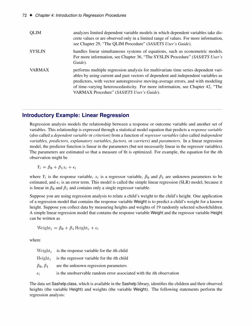
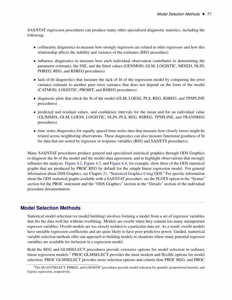
Figure 4.1 displays the default tabular output of PROC REG for this model. Nineteen observations are readfrom the data set, and all observations are used in the analysis. The estimates of the two regression parametersare b0 D �143:02692 and c1 D 3:89903. These estimates are obtained by the least squares principle. Formore information about the principle of least squares estimation and its role in linear model analysis, seethe sections “Classical Estimation Principles” and “Linear Model Theory” in Chapter 3, “Introduction toStatistical Modeling with SAS/STAT Software.” Also see an applied regression text such as Draper andSmith (1998); Daniel and Wood (1999); Johnston and DiNardo (1997); Weisberg (2005).
Figure 4.1 Regression for Weight and Height Data
The REG ProcedureModel: MODEL1
Dependent Variable: Weight
The REG ProcedureModel: MODEL1
Dependent Variable: Weight
Number of Observations Read 19
Number of Observations Used 19
Analysis of Variance
Source DFSum of
SquaresMean
Square F Value Pr > F
Model 1 7193.24912 7193.24912 57.08 <.0001
Error 17 2142.48772 126.02869
Corrected Total 18 9335.73684
Root MSE 11.22625 R-Square 0.7705
Dependent Mean 100.02632 Adj R-Sq 0.7570
Coeff Var 11.22330
Parameter Estimates
Variable DFParameter
EstimateStandard
Error t Value Pr > |t|
Intercept 1 -143.02692 32.27459 -4.43 0.0004
Height 1 3.89903 0.51609 7.55 <.0001
Based on the least squares estimates shown in Figure 4.1, the fitted regression line that relates height toweight is described by the equation
2Weight D �143:02692C 3:89903 �Height
The “hat” notation is used to emphasize that 2Weight is not one of the original observations but a valuepredicted under the regression model that has been fit to the data. In the least squares solution, the followingresidual sum of squares is minimized and the achieved criterion value is displayed in the analysis of variancetable as the error sum of squares (2142.48772):
SSE D19XiD1
.Weighti � ˇ0 � ˇ1Heighti /2
74 F Chapter 4: Introduction to Regression Procedures
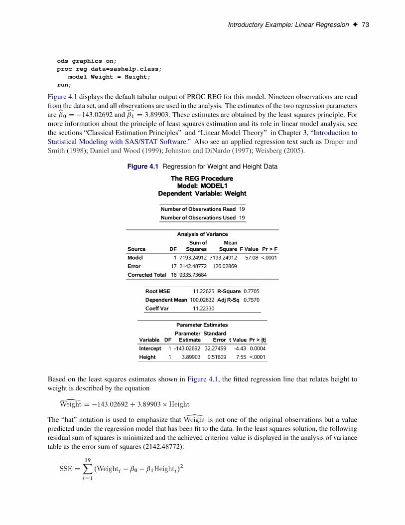
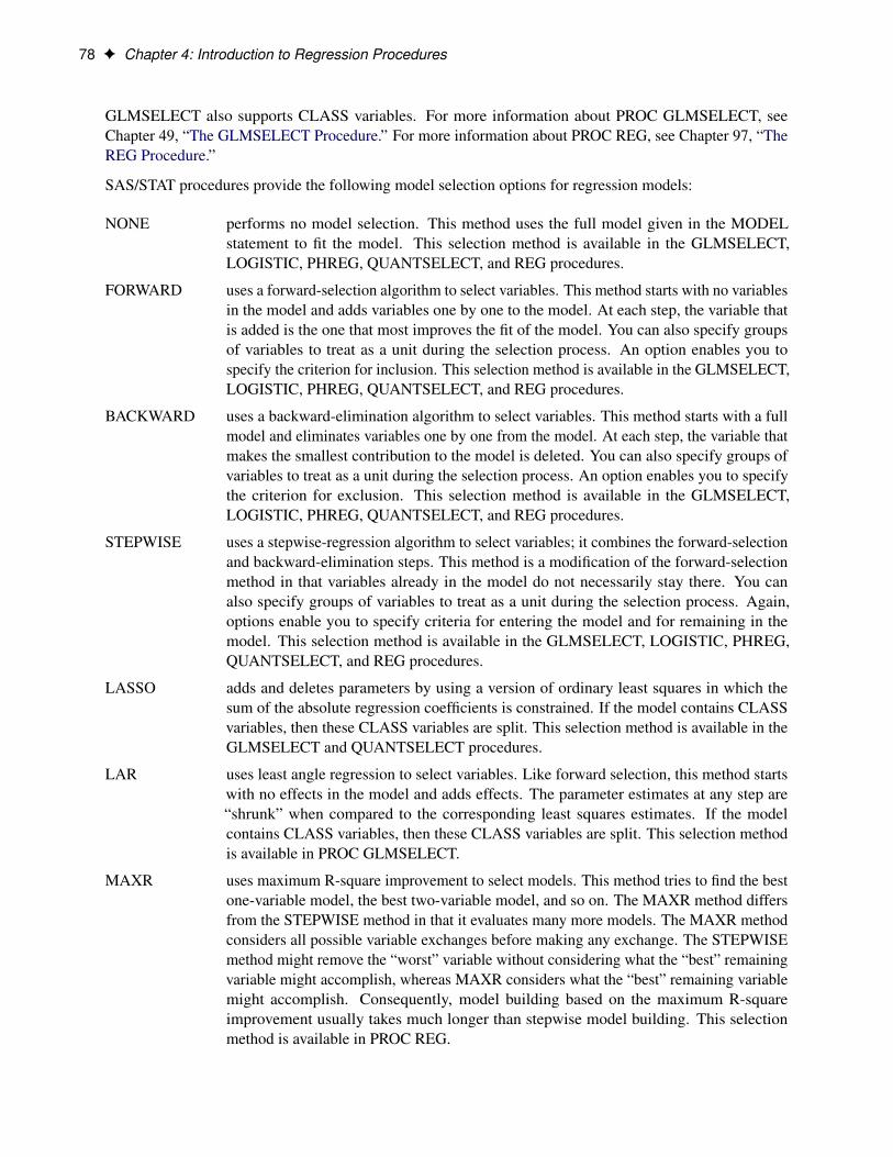
Figure 4.2 displays the fit plot that is produced by ODS Graphics. The fit plot shows the positive slope of thefitted line. The average weight of a child changes by b1 D 3:89903 units for each unit change in height. The95% confidence limits in the fit plot are pointwise limits that cover the mean weight for a particular heightwith probability 0.95. The prediction limits, which are wider than the confidence limits, show the pointwiselimits that cover a new observation for a given height with probability 0.95.
Figure 4.2 Fit Plot for Regression of Weight on Height
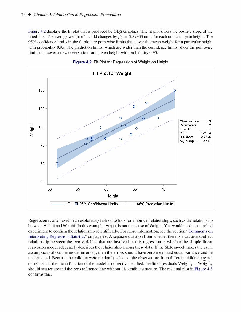
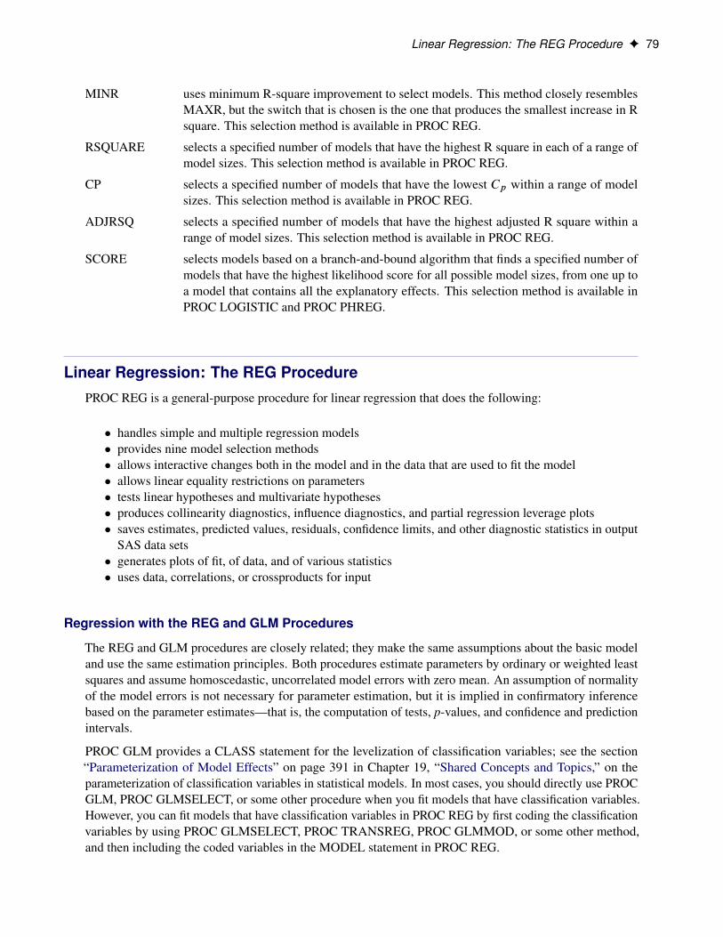
Regression is often used in an exploratory fashion to look for empirical relationships, such as the relationshipbetween Height and Weight. In this example, Height is not the cause of Weight. You would need a controlledexperiment to confirm the relationship scientifically. For more information, see the section “Comments onInterpreting Regression Statistics” on page 99. A separate question from whether there is a cause-and-effectrelationship between the two variables that are involved in this regression is whether the simple linearregression model adequately describes the relationship among these data. If the SLR model makes the usualassumptions about the model errors �i , then the errors should have zero mean and equal variance and beuncorrelated. Because the children were randomly selected, the observations from different children are notcorrelated. If the mean function of the model is correctly specified, the fitted residuals Weighti �2Weightishould scatter around the zero reference line without discernible structure. The residual plot in Figure 4.3confirms this.
Introductory Example: Linear Regression F 75
Figure 4.3 Residual Plot for Regression of Weight on Height
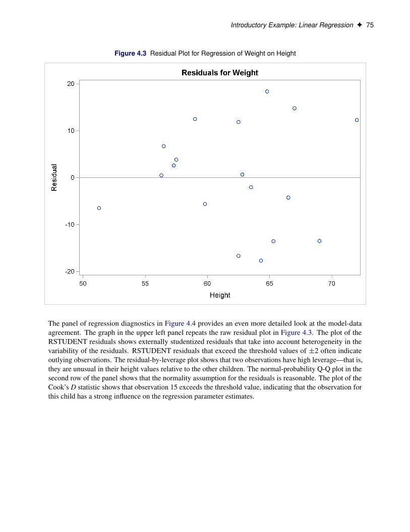
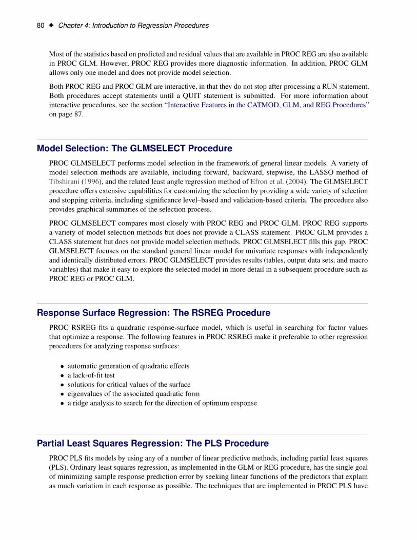
The panel of regression diagnostics in Figure 4.4 provides an even more detailed look at the model-dataagreement. The graph in the upper left panel repeats the raw residual plot in Figure 4.3. The plot of theRSTUDENT residuals shows externally studentized residuals that take into account heterogeneity in thevariability of the residuals. RSTUDENT residuals that exceed the threshold values of ˙2 often indicateoutlying observations. The residual-by-leverage plot shows that two observations have high leverage—that is,they are unusual in their height values relative to the other children. The normal-probability Q-Q plot in thesecond row of the panel shows that the normality assumption for the residuals is reasonable. The plot of theCook’s D statistic shows that observation 15 exceeds the threshold value, indicating that the observation forthis child has a strong influence on the regression parameter estimates.

76 F Chapter 4: Introduction to Regression Procedures
Figure 4.4 Panel of Regression Diagnostics
For more information about the interpretation of regression diagnostics and about ODS statistical graphicswith PROC REG, see Chapter 97, “The REG Procedure.”
SAS/STAT regression procedures produce the following information for a typical regression analysis:
� parameter estimates that are derived by using the least squares criterion� estimates of the variance of the error term� estimates of the variance or standard deviation of the sampling distribution of the parameter estimates� tests of hypotheses about the parameters
Model Selection Methods F 77
SAS/STAT regression procedures can produce many other specialized diagnostic statistics, including thefollowing:
� collinearity diagnostics to measure how strongly regressors are related to other regressors and how thisrelationship affects the stability and variance of the estimates (REG procedure)
� influence diagnostics to measure how each individual observation contributes to determining theparameter estimates, the SSE, and the fitted values (GENMOD, GLM, LOGISTIC, MIXED, NLIN,PHREG, REG, and RSREG procedures)
� lack-of-fit diagnostics that measure the lack of fit of the regression model by comparing the errorvariance estimate to another pure error variance that does not depend on the form of the model(CATMOD, LOGISTIC, PROBIT, and RSREG procedures)
� diagnostic plots that check the fit of the model (GLM, LOESS, PLS, REG, RSREG, and TPSPLINEprocedures)
� predicted and residual values, and confidence intervals for the mean and for an individual value(GLIMMIX, GLM, LOESS, LOGISTIC, NLIN, PLS, REG, RSREG, TPSPLINE, and TRANSREGprocedures)
� time series diagnostics for equally spaced time series data that measure how closely errors might berelated across neighboring observations. These diagnostics can also measure functional goodness of fitfor data that are sorted by regressor or response variables (REG and SAS/ETS procedures).
Many SAS/STAT procedures produce general and specialized statistical graphics through ODS Graphicsto diagnose the fit of the model and the model-data agreement, and to highlight observations that stronglyinfluence the analysis. Figure 4.2, Figure 4.3, and Figure 4.4, for example, show three of the ODS statisticalgraphs that are produced by PROC REG by default for the simple linear regression model. For generalinformation about ODS Graphics, see Chapter 21, “Statistical Graphics Using ODS.” For specific informationabout the ODS statistical graphs available with a SAS/STAT procedure, see the PLOTS option in the “Syntax”section for the PROC statement and the “ODS Graphics” section in the “Details” section of the individualprocedure documentation.
Model Selection MethodsStatistical model selection (or model building) involves forming a model from a set of regressor variablesthat fits the data well but without overfitting. Models are overfit when they contain too many unimportantregressor variables. Overfit models are too closely molded to a particular data set. As a result, overfit modelshave unstable regression coefficients and are quite likely to have poor predictive power. Guided, numericalvariable selection methods offer one approach to building models in situations where many potential regressorvariables are available for inclusion in a regression model.
Both the REG and GLMSELECT procedures provide extensive options for model selection in ordinarylinear regression models.1 PROC GLMSELECT provides the most modern and flexible options for modelselection. PROC GLMSELECT provides more selection options and criteria than PROC REG, and PROC
1The QUANTSELECT, PHREG, and LOGISTIC procedures provide model selection for quantile, proportional hazards, andlogistic regression, respectively.
78 F Chapter 4: Introduction to Regression Procedures
GLMSELECT also supports CLASS variables. For more information about PROC GLMSELECT, seeChapter 49, “The GLMSELECT Procedure.” For more information about PROC REG, see Chapter 97, “TheREG Procedure.”
SAS/STAT procedures provide the following model selection options for regression models:
NONE performs no model selection. This method uses the full model given in the MODELstatement to fit the model. This selection method is available in the GLMSELECT,LOGISTIC, PHREG, QUANTSELECT, and REG procedures.
FORWARD uses a forward-selection algorithm to select variables. This method starts with no variablesin the model and adds variables one by one to the model. At each step, the variable thatis added is the one that most improves the fit of the model. You can also specify groupsof variables to treat as a unit during the selection process. An option enables you tospecify the criterion for inclusion. This selection method is available in the GLMSELECT,LOGISTIC, PHREG, QUANTSELECT, and REG procedures.
BACKWARD uses a backward-elimination algorithm to select variables. This method starts with a fullmodel and eliminates variables one by one from the model. At each step, the variable thatmakes the smallest contribution to the model is deleted. You can also specify groups ofvariables to treat as a unit during the selection process. An option enables you to specifythe criterion for exclusion. This selection method is available in the GLMSELECT,LOGISTIC, PHREG, QUANTSELECT, and REG procedures.
STEPWISE uses a stepwise-regression algorithm to select variables; it combines the forward-selectionand backward-elimination steps. This method is a modification of the forward-selectionmethod in that variables already in the model do not necessarily stay there. You canalso specify groups of variables to treat as a unit during the selection process. Again,options enable you to specify criteria for entering the model and for remaining in themodel. This selection method is available in the GLMSELECT, LOGISTIC, PHREG,QUANTSELECT, and REG procedures.
LASSO adds and deletes parameters by using a version of ordinary least squares in which thesum of the absolute regression coefficients is constrained. If the model contains CLASSvariables, then these CLASS variables are split. This selection method is available in theGLMSELECT and QUANTSELECT procedures.
LAR uses least angle regression to select variables. Like forward selection, this method startswith no effects in the model and adds effects. The parameter estimates at any step are“shrunk” when compared to the corresponding least squares estimates. If the modelcontains CLASS variables, then these CLASS variables are split. This selection methodis available in PROC GLMSELECT.
MAXR uses maximum R-square improvement to select models. This method tries to find the bestone-variable model, the best two-variable model, and so on. The MAXR method differsfrom the STEPWISE method in that it evaluates many more models. The MAXR methodconsiders all possible variable exchanges before making any exchange. The STEPWISEmethod might remove the “worst” variable without considering what the “best” remainingvariable might accomplish, whereas MAXR considers what the “best” remaining variablemight accomplish. Consequently, model building based on the maximum R-squareimprovement usually takes much longer than stepwise model building. This selectionmethod is available in PROC REG.
Linear Regression: The REG Procedure F 79
MINR uses minimum R-square improvement to select models. This method closely resemblesMAXR, but the switch that is chosen is the one that produces the smallest increase in Rsquare. This selection method is available in PROC REG.
RSQUARE selects a specified number of models that have the highest R square in each of a range ofmodel sizes. This selection method is available in PROC REG.
CP selects a specified number of models that have the lowest Cp within a range of modelsizes. This selection method is available in PROC REG.
ADJRSQ selects a specified number of models that have the highest adjusted R square within arange of model sizes. This selection method is available in PROC REG.
SCORE selects models based on a branch-and-bound algorithm that finds a specified number ofmodels that have the highest likelihood score for all possible model sizes, from one up toa model that contains all the explanatory effects. This selection method is available inPROC LOGISTIC and PROC PHREG.
Linear Regression: The REG ProcedurePROC REG is a general-purpose procedure for linear regression that does the following:
� handles simple and multiple regression models� provides nine model selection methods� allows interactive changes both in the model and in the data that are used to fit the model� allows linear equality restrictions on parameters� tests linear hypotheses and multivariate hypotheses� produces collinearity diagnostics, influence diagnostics, and partial regression leverage plots� saves estimates, predicted values, residuals, confidence limits, and other diagnostic statistics in output
SAS data sets� generates plots of fit, of data, and of various statistics� uses data, correlations, or crossproducts for input
Regression with the REG and GLM Procedures
The REG and GLM procedures are closely related; they make the same assumptions about the basic modeland use the same estimation principles. Both procedures estimate parameters by ordinary or weighted leastsquares and assume homoscedastic, uncorrelated model errors with zero mean. An assumption of normalityof the model errors is not necessary for parameter estimation, but it is implied in confirmatory inferencebased on the parameter estimates—that is, the computation of tests, p-values, and confidence and predictionintervals.
PROC GLM provides a CLASS statement for the levelization of classification variables; see the section“Parameterization of Model Effects” on page 391 in Chapter 19, “Shared Concepts and Topics,” on theparameterization of classification variables in statistical models. In most cases, you should directly use PROCGLM, PROC GLMSELECT, or some other procedure when you fit models that have classification variables.However, you can fit models that have classification variables in PROC REG by first coding the classificationvariables by using PROC GLMSELECT, PROC TRANSREG, PROC GLMMOD, or some other method,and then including the coded variables in the MODEL statement in PROC REG.
80 F Chapter 4: Introduction to Regression Procedures
Most of the statistics based on predicted and residual values that are available in PROC REG are also availablein PROC GLM. However, PROC REG provides more diagnostic information. In addition, PROC GLMallows only one model and does not provide model selection.
Both PROC REG and PROC GLM are interactive, in that they do not stop after processing a RUN statement.Both procedures accept statements until a QUIT statement is submitted. For more information aboutinteractive procedures, see the section “Interactive Features in the CATMOD, GLM, and REG Procedures”on page 87.
Model Selection: The GLMSELECT ProcedurePROC GLMSELECT performs model selection in the framework of general linear models. A variety ofmodel selection methods are available, including forward, backward, stepwise, the LASSO method ofTibshirani (1996), and the related least angle regression method of Efron et al. (2004). The GLMSELECTprocedure offers extensive capabilities for customizing the selection by providing a wide variety of selectionand stopping criteria, including significance level–based and validation-based criteria. The procedure alsoprovides graphical summaries of the selection process.
PROC GLMSELECT compares most closely with PROC REG and PROC GLM. PROC REG supportsa variety of model selection methods but does not provide a CLASS statement. PROC GLM provides aCLASS statement but does not provide model selection methods. PROC GLMSELECT fills this gap. PROCGLMSELECT focuses on the standard general linear model for univariate responses with independentlyand identically distributed errors. PROC GLMSELECT provides results (tables, output data sets, and macrovariables) that make it easy to explore the selected model in more detail in a subsequent procedure such asPROC REG or PROC GLM.
Response Surface Regression: The RSREG ProcedurePROC RSREG fits a quadratic response-surface model, which is useful in searching for factor valuesthat optimize a response. The following features in PROC RSREG make it preferable to other regressionprocedures for analyzing response surfaces:
� automatic generation of quadratic effects� a lack-of-fit test� solutions for critical values of the surface� eigenvalues of the associated quadratic form� a ridge analysis to search for the direction of optimum response
Partial Least Squares Regression: The PLS ProcedurePROC PLS fits models by using any of a number of linear predictive methods, including partial least squares(PLS). Ordinary least squares regression, as implemented in the GLM or REG procedure, has the single goalof minimizing sample response prediction error by seeking linear functions of the predictors that explainas much variation in each response as possible. The techniques that are implemented in PROC PLS have
Generalized Linear Regression F 81
the additional goal of accounting for variation in the predictors under the assumption that directions inthe predictor space that are well sampled should provide better prediction for new observations when thepredictors are highly correlated. All the techniques that are implemented in PROC PLS work by extractingsuccessive linear combinations of the predictors, called factors (also called components or latent vectors),which optimally address one or both of these two goals—explaining response variation and explainingpredictor variation. In particular, the method of partial least squares balances the two objectives, seekingfactors that explain both response variation and predictor variation.
Generalized Linear RegressionAs outlined in the section “Generalized Linear Models” on page 33 in Chapter 3, “Introduction to StatisticalModeling with SAS/STAT Software,” the class of generalized linear models generalizes the linear regressionmodels in two ways:
� by allowing the data to come from a distribution that is a member of the exponential family ofdistributions
� by introducing a link function, g.�/, that provides a mapping between the linear predictor � D x0ˇ andthe mean of the data, g.EŒY �/ D �. The link function is monotonic, so that EŒY � D g�1.�/; g�1.�/ iscalled the inverse link function.
One of the most commonly used generalized linear regression models is the logistic model for binary orbinomial data. Suppose that Y denotes a binary outcome variable that takes on the values 1 and 0 with theprobabilities � and 1 � � , respectively. The probability � is also referred to as the “success probability,”supposing that the coding Y D 1 corresponds to a success in a Bernoulli experiment. The success probabilityis also the mean of Y, and one of the aims of logistic regression analysis is to study how regressor variablesaffect the outcome probabilities or functions thereof, such as odds ratios.
The logistic regression model for � is defined by the linear predictor � D x0ˇ and the logit link function:
logit.Pr.Y D 0// D log� �
1 � �
�D x0ˇ
The inversely linked linear predictor function in this model is
Pr.Y D 0/ D1
1C exp.��/
The dichotomous logistic regression model can be extended to multinomial (polychotomous) data. Twoclasses of models for multinomial data can be fit by using procedures in SAS/STAT software: models forordinal data that rely on cumulative link functions, and models for nominal (unordered) outcomes that rely ongeneralized logits. The next sections briefly discuss SAS/STAT procedures for logistic regression. For moreinformation about the comparison of the procedures mentioned there with respect to analysis of categoricalresponses, see Chapter 8, “Introduction to Categorical Data Analysis Procedures.”
The SAS/STAT procedures CATMOD, GENMOD, GLIMMIX, LOGISTIC, and PROBIT can fit generalizedlinear models for binary, binomial, and multinomial outcomes.
82 F Chapter 4: Introduction to Regression Procedures
Contingency Table Data: The CATMOD Procedure
PROC CATMOD fits models to data that are represented by a contingency table by using weighted leastsquares and a variety of link functions. Although PROC CATMOD also provides maximum likelihoodestimation for logistic regression, PROC LOGISTIC is more efficient for most analyses.
Generalized Linear Models: The GENMOD Procedure
PROC GENMOD is a generalized linear modeling procedure that estimates parameters by maximumlikelihood. It uses CLASS and MODEL statements to form the statistical model and can fit models to binaryand ordinal outcomes. The GENMOD procedure does not fit generalized logit models for nominal outcomes.However, PROC GENMOD can solve generalized estimating equations (GEE) to model correlated data andcan perform a Bayesian analysis.
Generalized Linear Mixed Models: The GLIMMIX Procedure
PROC GLIMMIX fits generalized linear mixed models. If the model does not contain random effects, PROCGLIMMIX fits generalized linear models by using the method of maximum likelihood. In the class of logisticregression models, PROC GLIMMIX can fit models to binary, binomial, ordinal, and nominal outcomes.
Logistic Regression: The LOGISTIC Procedure
PROC LOGISTIC fits logistic regression models and estimates parameters by maximum likelihood. Theprocedure fits the usual logistic regression model for binary data in addition to models with the cumulativelink function for ordinal data (such as the proportional odds model) and the generalized logit model fornominal data. PROC LOGISTIC offers a number of variable selection methods and can perform conditionaland exact conditional logistic regression analysis.
Discrete Event Data: The PROBIT Procedure
PROC PROBIT calculates maximum likelihood estimates of regression parameters and the natural (orthreshold) response rate for quantal response data from biological assays or other discrete event data. PROCPROBIT fits probit, logit, ordinal logistic, and extreme value (or gompit) regression models.
Correlated Data: The GENMOD and GLIMMIX Procedures
When a generalized linear model is formed by using distributions other than the binary, binomial, ormultinomial distribution, you can use the GENMOD and GLIMMIX procedures for parameter estimationand inference.
Both PROC GENMOD and PROC GLIMMIX can accommodate correlated observations, but they usedifferent techniques. PROC GENMOD fits correlated data models by using generalized estimating equationsthat rely on a first- and second-moment specification for the response data and a working correlationassumption. With PROC GLIMMIX, you can model correlations between the observations either byspecifying random effects in the conditional distribution that induce a marginal correlation structure or bydirect modeling of the marginal dependence. PROC GLIMMIX uses likelihood-based techniques to estimateparameters.
PROC GENMOD supports a Bayesian analysis through its BAYES statement.
With PROC GLIMMIX, you can vary the distribution or link function from one observation to the next.

Ill-Conditioned Data: The ORTHOREG Procedure F 83
To fit a generalized linear model by using a distribution that is not available in the GENMOD or GLIMMIXprocedure, you can use PROC NLMIXED and use SAS programming statements to code the log-likelihoodfunction of an observation.
Ill-Conditioned Data: The ORTHOREG ProcedurePROC ORTHOREG performs linear least squares regression by using the Gentleman-Givens computationalmethod (Gentleman 1972, 1973), and it can produce more accurate parameter estimates for ill-conditioneddata. PROC GLM and PROC REG produce very accurate estimates for most problems. However, if you havevery ill-conditioned data, consider using PROC ORTHOREG. The collinearity diagnostics in PROC REGcan help you determine whether PROC ORTHOREG would be useful.
Quantile Regression: The QUANTREG and QUANTSELECT ProceduresPROC QUANTREG models the effects of covariates on the conditional quantiles of a response variable byusing quantile regression. PROC QUANTSELECT performs quantile regression with model selection.
Ordinary least squares regression models the relationship between one or more covariates X and the con-ditional mean of the response variable EŒY jX D x�. Quantile regression extends the regression model toconditional quantiles of the response variable, such as the 90th percentile. Quantile regression is particularlyuseful when the rate of change in the conditional quantile, expressed by the regression coefficients, dependson the quantile. An advantage of quantile regression over least squares regression is its flexibility in modelingdata that have heterogeneous conditional distributions. Data of this type occur in many fields, includingbiomedicine, econometrics, and ecology.
Features of PROC QUANTREG include the following:
� simplex, interior point, and smoothing algorithms for estimation� sparsity, rank, and resampling methods for confidence intervals� asymptotic and bootstrap methods to estimate covariance and correlation matrices of the parameter
estimates� Wald and likelihood ratio tests for the regression parameter estimates� regression quantile spline fits
The QUANTSELECT procedure shares most of its syntax and output format with PROC GLMSELECT andPROC QUANTREG. Features of PROC QUANTSELECT include the following:
� a variety of selection methods, including forward, backward, stepwise, and LASSO� a variety of criteria, including AIC, AICC, ADJR1, SBC, significance level, testing ACL, and validation
ACL� effect selection both for individual quantile levels and for the entire quantile process� a SAS data set that contains the design matrix� macro variables that enable you to easily specify the selected model by using a subsequent PROC
QUANTREG step
84 F Chapter 4: Introduction to Regression Procedures
Nonlinear Regression: The NLIN and NLMIXED ProceduresRecall from Chapter 3, “Introduction to Statistical Modeling with SAS/STAT Software,” that a nonlinearregression model is a statistical model in which the mean function depends on the model parameters in anonlinear function. The SAS/STAT procedures that can fit general, nonlinear models are the NLIN andNLMIXED procedures. These procedures have the following similarities:
� Nonlinear models are fit by iterative methods.� You must provide an expression for the model by using SAS programming statements.� Analytic derivatives of the objective function with respect to the parameters are calculated automati-
cally.� A grid search is available to select the best starting values for the parameters from a set of starting
points that you provide.
The procedures have the following differences:
� PROC NLIN estimates parameters by using nonlinear least squares; PROC NLMIXED estimatesparameters by using maximum likelihood.
� PROC NLMIXED enables you to construct nonlinear models that contain normally distributed randomeffects.
� PROC NLIN requires that you declare all model parameters in the PARAMETERS statement and assignstarting values. PROC NLMIXED determines the parameters in your model from the PARAMETERstatement and the other modeling statements. It is not necessary to supply starting values for allparameters in PROC NLMIXED, but it is highly recommended.
� The residual variance is not a parameter in models that are fit by using PROC NLIN, but it is aparameter in models that are fit by using PROC NLMIXED.
� The default iterative optimization method in PROC NLIN is the Gauss-Newton method; the defaultmethod in PROC NLMIXED is the quasi-Newton method. Other optimization techniques are availablein both procedures.
Nonlinear models are fit by using iterative techniques that begin from starting values and attempt to iterativelyimprove on the estimates. There is no guarantee that the solution that is achieved when the iterative algorithmconverges will correspond to a global optimum.
Nonparametric RegressionParametric regression models express the mean of an observation as a function of the regressor variablesx1; : : : ; xk and the parameters ˇ1; : : : ; ˇp:
EŒY � D f .x1; : : : ; xkIˇ1; : : : ; ˇp/
Not only do nonparametric regression techniques relax the assumption of linearity in the regression parameters,but they also do not require that you specify a precise functional form for the relationship between response

Nonparametric Regression F 85
and regressor variables. Consider a regression problem in which the relationship between response Y andregressor X is to be modeled. It is assumed that EŒYi � D g.xi /C �i , where g.�/ is an unspecified regressionfunction. Two primary approaches in nonparametric regression modeling are as follows:
� Approximate g.xi / locally by a parametric function that is constructed from information in a localneighborhood of xi .
� Approximate the unknown function g.xi / by a smooth, flexible function and determine the necessarysmoothness and continuity properties from the data.
The SAS/STAT procedures ADAPTIVEREG, LOESS, TPSPLINE, and GAM fit nonparametric regressionmodels by one of these methods.
Adaptive Regression: The ADAPTIVEREG Procedure
PROC ADAPTIVEREG fits multivariate adaptive regression splines as defined by Friedman (1991). Themethod is a nonparametric regression technique that combines regression splines and model selection methods.It does not assume parametric model forms and does not require specification of knot values for constructingregression spline terms. Instead, it constructs spline basis functions in an adaptive way by automaticallyselecting appropriate knot values for different variables and obtains reduced models by applying modelselection techniques. PROC ADAPTIVEREG supports models that contain classification variables.
Local Regression: The LOESS Procedure
PROC LOESS implements a local regression approach for estimating regression surfaces that was pioneeredby Cleveland, Devlin, and Grosse (1988). No assumptions about the parametric form of the entire regressionsurface are made by PROC LOESS. Only a parametric form of the local approximation is specified by theuser. Furthermore, PROC LOESS is suitable when there are outliers in the data and a robust fitting method isnecessary.
Thin Plate Smoothing Splines: The TPSPLINE Procedure
PROC TPSPLINE decomposes the regressor contributions to the mean function into parametric componentsand into smooth functional components. Suppose that the regressor variables are collected into the vector xand that this vector is partitioned as x D Œx01 x02�
0. The relationship between Y and x2 is linear (parametric),and the relationship between Y and x1 is nonparametric. PROC TPSPLINE fits models of the form
EŒY � D g.x1/C x02ˇ
The function g.�/ can be represented as a sequence of spline basis functions.
The parameters are estimated by a penalized least squares method. The penalty is applied to the usual leastsquares criterion to obtain a regression estimate that fits the data well and to prevent the fit from attemptingto interpolate the data (fit the data too closely).
Generalized Additive Models: The GAM Procedure
Generalized additive models are nonparametric models in which one or more regressor variables are presentand can make different smooth contributions to the mean function. For example, if xi D Œxi1; xi2; : : : ; xik�

86 F Chapter 4: Introduction to Regression Procedures
is a vector of k regressor for the ith observation, then an additive model represents the mean function as
EŒY � D f0 C f1.xi1/C f2.xi2/C � � � C f3.xi3/
The individual functions fj can have a parametric or nonparametric form. If all fj are parametric, PROCGAM fits a fully parametric model. If some fj are nonparametric, PROC GAM fits a semiparametric model.Otherwise, the models are fully nonparametric.
The generalization of additive models is akin to the generalization for linear models: nonnormal data areaccommodated by explicitly modeling the distribution of the data as a member of the exponential family andby applying a monotonic link function that provides a mapping between the predictor and the mean of thedata.
Robust Regression: The ROBUSTREG ProcedurePROC ROBUSTREG implements algorithms to detect outliers and provide resistant (stable) results inthe presence of outliers. The ROBUSTREG procedure provides four such methods: M estimation, LTSestimation, S estimation, and MM estimation.
� M estimation, which was introduced by Huber (1973), is the simplest approach both computationallyand theoretically. Although it is not robust with respect to leverage points, it is still used extensively inanalyzing data for which it can be assumed that the contamination is mainly in the response direction.
� Least trimmed squares (LTS) estimation is a high breakdown value method that was introduced byRousseeuw (1984). The breakdown value is a measure of the proportion of observations that arecontaminated by outliers that an estimation method can withstand and still maintain its robustness.
� S estimation is a high breakdown value method that was introduced by Rousseeuw and Yohai (1984).When the breakdown value is the same, it has a higher statistical efficiency than LTS estimation.
� MM estimation, which was introduced by Yohai (1987), combines high breakdown value estimationand M estimation. It has the high breakdown property of S estimation but a higher statistical efficiency.
For diagnostic purposes, PROC ROBUSTREG also implements robust leverage-point detection based on therobust Mahalanobis distance. The robust distance is computed by using a generalized minimum covariancedeterminant (MCD) algorithm.
Regression with Transformations: The TRANSREG ProcedurePROC TRANSREG fits linear models to data. In addition, PROC TRANSREG can find nonlinear transfor-mations of the data and fit a linear model to the transformed data. This is in contrast to PROC REG andPROC GLM, which fit linear models to data, and PROC NLIN, which fits nonlinear models to data. PROCTRANSREG fits a variety of models, including the following:
� ordinary regression and ANOVA� metric and nonmetric conjoint analysis
Interactive Features in the CATMOD, GLM, and REG Procedures F 87
� metric and nonmetric vector and ideal point preference mapping� simple, multiple, and multivariate regression with optional variable transformations� redundancy analysis with optional variable transformations� canonical correlation analysis with optional variable transformations� simple and multiple regression models with a Box-Cox (1964) transformation of the dependent variable� regression models with penalized B-splines (Eilers and Marx 1996)
Interactive Features in the CATMOD, GLM, and REG ProceduresThe CATMOD, GLM, and REG procedures are interactive: they do not stop after processing a RUN statement.You can submit more statements to continue the analysis that was started by the previous statements. Bothinteractive and noninteractive procedures stop if a DATA step, a new procedure step, or a QUIT or ENDSASstatement is submitted. Noninteractive SAS procedures also stop if a RUN statement is submitted.
Placement of statements is critical in interactive procedures, particularly for ODS statements. For example, ifyou submit the following steps, no ODS OUTPUT data set is created:
proc reg data=sashelp.class;model weight = height;
run;
ods output parameterestimates=pm;proc glm data=sashelp.class;
class sex;model weight = sex | height / solution;
run;
You can cause the PROC GLM step to create an output data set by adding a QUIT statement to the PROCREG step or by moving the ODS OUTPUT statement so that it follows the PROC GLM statement. Formore information about the placement of RUN, QUIT, and ODS statements in interactive procedures, seeExample 20.6 in Chapter 20, “Using the Output Delivery System.”
Statistical Background in Linear RegressionThe remainder of this chapter outlines the way in which many SAS/STAT regression procedures calculatevarious regression quantities. The discussion focuses on the linear regression models. For general statisticalbackground about linear statistical models, see the section “Linear Model Theory” in Chapter 3, “Introductionto Statistical Modeling with SAS/STAT Software.”
Exceptions and further details are documented for individual procedures.
Linear Regression ModelsIn matrix notation, a linear model is written as
Y D Xˇ C �
88 F Chapter 4: Introduction to Regression Procedures
where X is the .n� k/ design matrix (rows are observations and columns are the regressors), ˇ is the .k � 1/vector of unknown parameters, and � is the .n � 1/ vector of unobservable model errors. The first column ofX is usually a vector of 1s and is used to estimate the intercept term.
The statistical theory of linear models is based on strict classical assumptions. Ideally, you measure theresponse after controlling all factors in an experimentally determined environment. If you cannot control thefactors experimentally, some tests must be interpreted as being conditional on the observed values of theregressors.
Other assumptions are as follows:
� The form of the model is correct (all important explanatory variables have been included). Thisassumption is reflected mathematically in the assumption of a zero mean of the model errors, EŒ�� D 0.
� Regressor variables are measured without error.
� The expected value of the errors is 0.
� The variance of the error (and thus the dependent variable) for the ith observation is �2=wi , where wiis a known weight factor. Usually, wi D 1 for all i and thus �2 is the common, constant variance.
� The errors are uncorrelated across observations.
When hypotheses are tested, or when confidence and prediction intervals are computed, an additionalassumption is made that the errors are normally distributed.
Parameter Estimates and Associated Statistics
Least Squares Estimators
Least squares estimators of the regression parameters are found by solving the normal equations�X0WX
�ˇ D X0WY
for the vector ˇ, where W is a diagonal matrix of observed weights. The resulting estimator of the parametervector is
bD �X0WX��1 X0WY
This is an unbiased estimator, because
Ehbi D �X0WX
��1 X0WEŒY�
D�X0WX
��1 X0WXˇ D ˇ
Notice that the only assumption necessary in order for the least squares estimators to be unbiased is that of azero mean of the model errors. If the estimator is evaluated at the observed data, it is referred to as the leastsquares estimate,
bD �X0WX��1 X0WY
Parameter Estimates and Associated Statistics F 89
If the standard classical assumptions are met, the least squares estimators of the regression parameters are thebest linear unbiased estimators (BLUE). In other words, the estimators have minimum variance in the classof estimators that are unbiased and that are linear functions of the responses. If the additional assumption ofnormally distributed errors is satisfied, then the following are true:
� The statistics that are computed have the proper sampling distributions for hypothesis testing.
� Parameter estimators are normally distributed.
� Various sums of squares are distributed proportional to chi-square, at least under proper hypotheses.
� Ratios of estimators to standard errors follow the Student’s t distribution under certain hypotheses.
� Appropriate ratios of sums of squares follow an F distribution for certain hypotheses.
When regression analysis is used to model data that do not meet the assumptions, you should interpretthe results in a cautious, exploratory fashion. The significance probabilities under these circumstances areunreliable.
Box (1966) and Mosteller and Tukey (1977, Chapters 12 and 13) discuss the problems that are encounteredin regression data, especially when the data are not under experimental control.
Estimating the Precision
Assume for the present that X0WX has full column rank k (this assumption is relaxed later). The variance ofthe error terms, VarŒ�i � D �2, is then estimated by the mean square error,
s2 D MSE DSSEn � k
D1
n � k
nXiD1
wi�yi � x0iˇ
�2where x0i is the ith row of the design matrix X. The residual variance estimate is also unbiased: EŒs2� D �2.
The covariance matrix of the least squares estimators is
Varhbi D �2 �X0WX
��1An estimate of the covariance matrix is obtained by replacing �2 with its estimate, s2 in the precedingformula. This estimate is often referred to as COVB in SAS/STAT modeling procedures:
COVB DbVarhbi D s2 �X0WX
��1The correlation matrix of the estimates, often referred to as CORRB, is derived by scaling the covariance
matrix: Let S D diag��
X0WX��1�� 1
2. Then the correlation matrix of the estimates is
CORRB D S�X0WX
��1 S
The estimated standard error of the ith parameter estimator is obtained as the square root of the ith diagonalelement of the COVB matrix. Formally,
STDERR�b
i
�D
q�s2.X0WX/�1
�i i
90 F Chapter 4: Introduction to Regression Procedures
The ratio
t Dbi
STDERR�b
i
�follows a Student’s t distribution with .n � k/ degrees of freedom under the hypothesis that ˇi is zero andprovided that the model errors are normally distributed.
Regression procedures display the t ratio and the significance probability, which is the probability under thehypothesis H Wˇi D 0 of a larger absolute t value than was actually obtained. When the probability is lessthan some small level, the event is considered so unlikely that the hypothesis is rejected.
Type I SS and Type II SS measure the contribution of a variable to the reduction in SSE. Type I SS measurethe reduction in SSE as that variable is entered into the model in sequence. Type II SS are the incrementin SSE that results from removing the variable from the full model. Type II SS are equivalent to the TypeIII and Type IV SS that are reported in PROC GLM. If Type II SS are used in the numerator of an F test,the test is equivalent to the t test for the hypothesis that the parameter is zero. In polynomial models, Type ISS measure the contribution of each polynomial term after it is orthogonalized to the previous terms in themodel. The four types of SS are described in Chapter 15, “The Four Types of Estimable Functions.”
Coefficient of Determination
The coefficient of determination in a regression model, also known as the R-square statistic, measures theproportion of variability in the response that is explained by the regressor variables. In a linear regressionmodel with intercept, R square is defined as
R2 D 1 �SSESST
where SSE is the residual (error) sum of squares and SST is the total sum of squares corrected for the mean.The adjusted R-square statistic is an alternative to R square that takes into account the number of parametersin the model. The adjusted R-square statistic is calculated as
ADJRSQ D 1 �n � i
n � p
�1 �R2
�where n is the number of observations that are used to fit the model, p is the number of parameters in themodel (including the intercept), and i is 1 if the model includes an intercept term, and 0 otherwise.
R-square statistics also play an important indirect role in regression calculations. For example, the proportionof variability that is explained by regressing all other variables in a model on a particular regressor canprovide insights into the interrelationship among the regressors.
Tolerances and variance inflation factors measure the strength of interrelationships among the regressorvariables in the model. If all variables are orthogonal to each other, both tolerance and variance inflationare 1. If a variable is very closely related to other variables, the tolerance approaches 0 and the varianceinflation gets very large. Tolerance (TOL) is 1 minus the R square that results from the regression of the othervariables in the model on that regressor. Variance inflation (VIF) is the diagonal of .X0WX/�1, if .X0WX/ isscaled to correlation form. The statistics are related as
VIF D1
TOL
Parameter Estimates and Associated Statistics F 91
Explicit and Implicit Intercepts
A linear model contains an explicit intercept if the X matrix contains a column whose nonzero values do notvary, usually a column of ones. Many SAS/STAT procedures automatically add this column of ones as thefirst column in the X matrix. Procedures that support a NOINT option in the MODEL statement provide thecapability to suppress the automatic addition of the intercept column.
In general, models without an intercept should be the exception, especially if your model does not containclassification (CLASS) variables. An overall intercept is provided in many models to adjust for the grandtotal or overall mean in your data. A simple linear regression without intercept, such as
EŒYi � D ˇ1xi C �i
assumes that Y has mean zero if X takes on the value zero. This might not be a reasonable assumption.
If you explicitly suppress the intercept in a statistical model, the calculation and interpretation of your resultscan change. For example, the exclusion of the intercept in the following PROC REG statements leads toa different calculation of the R-square statistic. It also affects the calculation of the sum of squares in theanalysis of variance for the model. For example, the model and error sum of squares add up to the uncorrectedtotal sum of squares in the absence of an intercept.
proc reg;model y = x / noint;
quit;
Many statistical models contain an implicit intercept, which occurs when a linear function of one or morecolumns in the X matrix produces a column of constant, nonzero values. For example, the presence of aCLASS variable in the GLM parameterization always implies an intercept in the model. If a model containsan implicit intercept, then adding an intercept to the model does not alter the quality of the model fit, but itchanges the interpretation (and number) of the parameter estimates.
The way in which the implicit intercept is detected and accounted for in the analysis depends on the procedure.For example, the following statements in PROC GLM lead to an implied intercept:
proc glm;class a;model y = a / solution noint;
run;
Whereas the analysis of variance table uses the uncorrected total sum of squares (because of the NOINToption), the implied intercept does not lead to a redefinition or recalculation of the R-square statistic(compared to the model without the NOINT option). Also, because the intercept is implied by the presenceof the CLASS variable a in the model, the same error sum of squares results whether the NOINT option isspecified or not.
A different approach is taken, for example, by PROC TRANSREG. The ZERO=NONE option in the CLASSparameterization of the following statements leads to an implicit intercept model:
proc transreg;model ide(y) = class(a / zero=none) / ss2;
run;
The analysis of variance table or the regression fit statistics are not affected in PROC TRANSREG. Only theinterpretation of the parameter estimates changes because of the way in which the intercept is accounted forin the model.
92 F Chapter 4: Introduction to Regression Procedures
Implied intercepts not only occur when classification effects are present in the model. They also occur withB-splines and other sets of constructed columns.
Models Not of Full Rank
If the X matrix is not of full rank, then a generalized inverse can be used to solve the normal equations tominimize the SSE:
bD �X0WX��X0WY
However, these estimates are not unique, because there are an infinite number of solutions that correspond todifferent generalized inverses. PROC REG and other regression procedures choose a nonzero solution forall variables that are linearly independent of previous variables and a zero solution for other variables. Thisapproach corresponds to using a generalized inverse in the normal equations, and the expected values of theestimates are the Hermite normal form of X0WX multiplied by the true parameters:
Ehbi D �X0WX
��.X0WX/ˇ
Degrees of freedom for the estimates that correspond to singularities are not counted (reported as zero). Thehypotheses that are not testable have t tests displayed as missing. The message that the model is not of fullrank includes a display of the relations that exist in the matrix.
For information about generalized inverses and their importance for statistical inference in linear models,see the sections “Generalized Inverse Matrices” and “Linear Model Theory” in Chapter 3, “Introduction toStatistical Modeling with SAS/STAT Software.”
Predicted and Residual ValuesAfter the model has been fit, predicted and residual values are usually calculated, graphed, and output. Thepredicted values are calculated from the estimated regression equation; the raw residuals are calculatedas the observed value minus the predicted value. Often other forms of residuals, such as studentized orcumulative residuals, are used for model diagnostics. Some procedures can calculate standard errors ofresiduals, predicted mean values, and individual predicted values.
Consider the ith observation, where x0i is the row of regressors, b is the vector of parameter estimates, and s2
is the estimate of the residual variance (the mean squared error). The leverage value of the ith observation isdefined as
hi D wix0i .X0WX/�1xi
where X is the design matrix for the observed data, x0i is an arbitrary regressor vector (possibly but notnecessarily a row of X), W is a diagonal matrix of observed weights, and wi is the weight corresponding tox0i .
Then the predicted mean and the standard error of the predicted mean are
byi D x0ibSTDERR.byi / Dqs2hi=wi
Predicted and Residual Values F 93
The standard error of the individual (future) predicted value yi is
STDERR.yi / Dqs2.1C hi /=wi
If the predictor vector xi corresponds to an observation in the analysis data, then the raw residual for thatobservation and the standard error of the raw residual are defined as
RESIDi D yi � x0ibSTDERR.RESIDi / D
qs2.1 � hi /=wi
The studentized residual is the ratio of the raw residual and its estimated standard error. Symbolically,
STUDENTi DRESIDi
STDERR.RESIDi /
Two types of intervals provide a measure of confidence for prediction: the confidence interval for the meanvalue of the response, and the prediction (or forecasting) interval for an individual observation. As discussedin the section “Mean Squared Error” in Chapter 3, “Introduction to Statistical Modeling with SAS/STATSoftware,” both intervals are based on the mean squared error of predicting a target based on the resultof the model fit. The difference in the expressions for the confidence interval and the prediction intervaloccurs because the target of estimation is a constant in the case of the confidence interval (the mean of anobservation) and the target is a random variable in the case of the prediction interval (a new observation).
For example, you can construct a confidence interval for the ith observation that contains the true mean valueof the response with probability 1 � ˛. The upper and lower limits of the confidence interval for the meanvalue are
LowerM D x0ib� t˛=2;�qs2hi=wiUpperM D x0ibC t˛=2;�qs2hi=wi
where t˛=2;� is the tabulated t quantile with degrees of freedom equal to the degrees of freedom for the meansquared error, � D n � rank.X/.
The limits for the prediction interval for an individual response are
LowerI D x0ib� t˛=2;�qs2.1C hi /=wiUpperI D x0ibC t˛=2;�qs2.1C hi /=wi
Influential observations are those that, according to various criteria, appear to have a large influence on theanalysis. One measure of influence, Cook’s D, measures the change to the estimates that results from deletingan observation,
COOKDi D1
kSTUDENT2i
�STDERR.byi /
STDERR.RESIDi /
�2where k is the number of parameters in the model (including the intercept). For more information, see Cook(1977, 1979).
94 F Chapter 4: Introduction to Regression Procedures
The predicted residual for observation i is defined as the residual for the ith observation that results fromdropping the ith observation from the parameter estimates. The sum of squares of predicted residual errors iscalled the PRESS statistic:
PRESIDi DRESIDi1 � hi
PRESS DnXiD1
wiPRESID2i
Testing Linear HypothesesTesting of linear hypotheses based on estimable functions is discussed in the section “Test of Hypotheses” onpage 59 in Chapter 3, “Introduction to Statistical Modeling with SAS/STAT Software,” and the constructionof special sets of estimable functions corresponding to Type I–Type IV hypotheses is discussed in Chapter 15,“The Four Types of Estimable Functions.” In linear regression models, testing of general linear hypothesesfollows along the same lines. Test statistics are usually formed based on sums of squares that are associatedwith the hypothesis in question. Furthermore, when X is of full rank—as is the case in many regressionmodels—the consistency of the linear hypothesis is guaranteed.
Recall from Chapter 3, “Introduction to Statistical Modeling with SAS/STAT Software,” that the generalform of a linear hypothesis for the parameters is H WLˇ D d, where L is q � k, ˇ is k � 1, and d is q � 1. Totest this hypothesis, you take the linear function with respect to the parameter estimates: Lb� d. This linearfunction in b has variance
VarhLbi D LVarŒb�L0 D �2L
�X0WX
�� L0
The sum of squares due to the hypothesis is a simple quadratic form:
SS.H/ D SS.Lb� d/ D�
Lb� d�0 �
L�X0WX
�� L0��1 �Lb� d
�If this hypothesis is testable, then SS.H/ can be used in the numerator of an F statistic:
F DSS.H/=q
s2D
SS.Lb � d/=qs2
If b is normally distributed, which follows as a consequence of normally distributed model errors, then thisstatistic follows an F distribution with q numerator degrees of freedom and n� rank.X/ denominator degreesof freedom. Note that it was assumed in this derivation that L is of full row rank q.
Multivariate TestsMultivariate hypotheses involve several dependent variables in the form
H WLˇM D d

Multivariate Tests F 95
where L is a linear function on the regressor side, ˇ is a matrix of parameters, M is a linear function onthe dependent side, and d is a matrix of constants. The special case (handled by PROC REG) in which theconstants are the same for each dependent variable is expressed as
.Lˇ � cj/M D 0
where c is a column vector of constants and j is a row vector of 1s. The special case in which the constantsare 0 is then
LˇM D 0
These multivariate tests are covered in detail in Morrison (2004); Timm (2002); Mardia, Kent, and Bibby(1979); Bock (1975); and other works cited in Chapter 9, “Introduction to Multivariate Procedures.”
Notice that in contrast to the tests discussed in the preceding section, ˇ here is a matrix of parameter estimates.Suppose that the matrix of estimates is denoted as B. To test the multivariate hypothesis, construct twomatrices, H and E, that correspond to the numerator and denominator of a univariate F test:
H DM0.LB � cj/0.L.X0WX/�L0/�1.LB � cj/ME DM0
�Y0WY � B0.X0WX/B
�M
Four test statistics, based on the eigenvalues of E�1H or .ECH/�1H, are formed. Let �i be the orderedeigenvalues of E�1H (if the inverse exists), and let �i be the ordered eigenvalues of .ECH/�1H. It happensthat �i D �i=.1C �i / and �i D �i=.1 � �i /, and it turns out that �i D
p�i is the ith canonical correlation.
Let p be the rank of .HC E/, which is less than or equal to the number of columns of M. Let q be the rankof L.X0WX/�L0. Let v be the error degrees of freedom, and let s D min.p; q/. Let m D .jp � qj � 1/=2,and let n D .v � p � 1/=2. Then the following statistics test the multivariate hypothesis in various ways, andtheir p-values can be approximated by F distributions. Note that in the special case that the rank of H is 1, allthese F statistics are the same and the corresponding p-values are exact, because in this case the hypothesis isreally univariate.
Wilks’ Lambda
If
ƒ Ddet.E/
det.HC E/D
nYiD1
1
1C �iD
nYiD1
.1 � �i /
then
F D1 �ƒ1=t
ƒ1=t�rt � 2u
pq
is approximately F distributed, where
r Dv �p � q C 1
2
u Dpq � 2
4
t D
( qp2q2�4
p2Cq2�5ifp2 C q2 � 5 > 0
1 otherwise
The degrees of freedom are pq and rt � 2u. The distribution is exact if min.p; q/ � 2. (See Rao 1973, p.556.)
96 F Chapter 4: Introduction to Regression Procedures
Pillai’s Trace
If
V D trace�H.HC E/�1
�D
nXiD1
�i
1C �iD
nXiD1
�i
then
F D2nC s C 1
2mC s C 1�V
s � V
is approximately F distributed with s.2mC s C 1/ and s.2nC s C 1/ degrees of freedom.
Hotelling-Lawley Trace
If
U D trace�E�1H
�D
nXiD1
�i D
nXiD1
�i
1 � �i
then for n > 0
F D .U=c/..4C .pq C 2/=.b � 1//=.pq//
is approximately F distributed with pq and 4C .pq C 2/=.b � 1/ degrees of freedom, where b D .p C
2n/.q C 2n/=.2.2nC 1/.n � 1// and c D .2C .pq C 2/=.b � 1//=.2n/; while for n � 0
F D2.snC 1/U
s2.2mC s C 1/
is approximately F with s.2mC s C 1/ and 2.snC 1/ degrees of freedom.
Roy’s Maximum Root
If ‚ D �1, then
F D ‚v � r C q
r
where r D max.p; q/ is an upper bound on F that yields a lower bound on the significance level. Degrees offreedom are r for the numerator and v � r C q for the denominator.
Tables of critical values for these statistics are found in Pillai (1960).
Exact Multivariate Tests
If you specify the MSTAT=EXACT option in the appropriate statement, p-values for three of the four tests(Wilks’ lambda, the Hotelling-Lawley trace, and Roy’s greatest root) are computed exactly, and the p-valuesfor the fourth test (Pillai’s trace) are based on an F approximation that is more accurate (but occasionallyslightly more liberal) than the default. The exact p-values for Roy’s greatest root benefit the most, because inthis case the F approximation provides only a lower bound for the p-value. If you use the F-based p-value forthis test in the usual way, declaring a test significant if p < 0.05, then your decisions might be very liberal. Forexample, instead of the nominal 5% Type I error rate, such a procedure can easily have an actual Type I error
Multivariate Tests F 97
rate in excess of 30%. By contrast, basing such a procedure on the exact p-values results in the appropriate5% Type I error rate, under the usual regression assumptions.
The MSTAT=EXACT option is supported in the ANOVA, CANCORR, CANDISC, GLM, and REG proce-dures.
The exact p-values are based on the following sources:
� Wilks’ lambda: Lee (1972); Davis (1979)
� Pillai’s trace: Muller (1998)
� Hotelling-Lawley trace: Davis (1970, 1980)
� Roy’s greatest root: Davis (1972); Pillai and Flury (1984)
Note that, although the MSTAT=EXACT p-value for Pillai’s trace is still approximate, it has “substantiallygreater accuracy” than the default approximation (Muller 1998).
Because most of the MSTAT=EXACT p-values are not based on the F distribution, the columns in themultivariate tests table that correspond to this approximation—in particular, the F value and the numeratorand denominator degrees of freedom—are no longer displayed, and the column that contains the p-valuesis labeled “P Value” instead of “Pr > F.” Suppose, for example, that you use the following PROC ANOVAstatements to perform a multivariate analysis of an archaeological data set:
data Skulls;input Loc $20. Basal Occ Max;datalines;
Minas Graes, Brazil 2.068 2.070 1.580Minas Graes, Brazil 2.068 2.074 1.602Minas Graes, Brazil 2.090 2.090 1.613Minas Graes, Brazil 2.097 2.093 1.613Minas Graes, Brazil 2.117 2.125 1.663Minas Graes, Brazil 2.140 2.146 1.681Matto Grosso, Brazil 2.045 2.054 1.580Matto Grosso, Brazil 2.076 2.088 1.602Matto Grosso, Brazil 2.090 2.093 1.643Matto Grosso, Brazil 2.111 2.114 1.643Santa Cruz, Bolivia 2.093 2.098 1.653Santa Cruz, Bolivia 2.100 2.106 1.623Santa Cruz, Bolivia 2.104 2.101 1.653;
proc anova data=Skulls;class Loc;model Basal Occ Max = Loc / nouni;manova h=Loc;ods select MultStat;
run;
The default multivariate tests, based on the F approximations, are shown in Figure 4.5
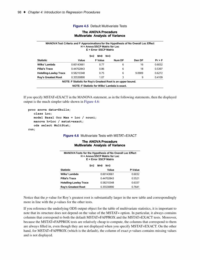
98 F Chapter 4: Introduction to Regression Procedures
Figure 4.5 Default Multivariate Tests
The ANOVA ProcedureMultivariate Analysis of Variance
The ANOVA ProcedureMultivariate Analysis of Variance
MANOVATest Criteria and F Approximations for the Hypothesis of No Overall Loc EffectH = Anova SSCP Matrix for Loc
E = Error SSCP Matrix
S=2 M=0 N=3
Statistic Value F Value Num DF Den DF Pr > F
Wilks' Lambda 0.60143661 0.77 6 16 0.6032
Pillai's Trace 0.44702843 0.86 6 18 0.5397
Hotelling-Lawley Trace 0.58210348 0.75 6 9.0909 0.6272
Roy's Greatest Root 0.35530890 1.07 3 9 0.4109
NOTE: F Statistic for Roy's Greatest Root is an upper bound.
NOTE: F Statistic for Wilks' Lambda is exact.
If you specify MSTAT=EXACT in the MANOVA statement, as in the following statements, then the displayedoutput is the much simpler table shown in Figure 4.6:
proc anova data=Skulls;class Loc;model Basal Occ Max = Loc / nouni;manova h=Loc / mstat=exact;ods select MultStat;
run;
Figure 4.6 Multivariate Tests with MSTAT=EXACT
The ANOVA ProcedureMultivariate Analysis of Variance
The ANOVA ProcedureMultivariate Analysis of Variance
MANOVATests for the Hypothesis of No Overall Loc EffectH = Anova SSCP Matrix for Loc
E = Error SSCP Matrix
S=2 M=0 N=3
Statistic Value P-Value
Wilks' Lambda 0.60143661 0.6032
Pillai's Trace 0.44702843 0.5521
Hotelling-Lawley Trace 0.58210348 0.6337
Roy's Greatest Root 0.35530890 0.7641
Notice that the p-value for Roy’s greatest root is substantially larger in the new table and correspondinglymore in line with the p-values for the other tests.
If you reference the underlying ODS output object for the table of multivariate statistics, it is important tonote that its structure does not depend on the value of the MSTAT= option. In particular, it always containscolumns that correspond to both the default MSTAT=FAPPROX and the MSTAT=EXACT tests. Moreover,because the MSTAT=FAPPROX tests are relatively cheap to compute, the columns that correspond to themare always filled in, even though they are not displayed when you specify MSTAT=EXACT. On the otherhand, for MSTAT=FAPPROX (which is the default), the column of exact p-values contains missing valuesand is not displayed.
Comments on Interpreting Regression Statistics F 99
Comments on Interpreting Regression StatisticsIn most applications, regression models are merely useful approximations. Reality is often so complicatedthat you cannot know what the true model is. You might have to choose a model more on the basis of whatvariables can be measured and what kinds of models can be estimated than on a rigorous theory that explainshow the universe really works. However, even in cases where theory is lacking, a regression model canbe an excellent predictor of the response if the model is carefully formulated from a large sample. Theinterpretation of statistics such as parameter estimates might nevertheless be highly problematic.
Statisticians usually use the word “prediction” in a technical sense. Prediction in this sense does not referto “predicting the future” (statisticians call that forecasting) but rather to guessing the response from thevalues of the regressors in an observation taken under the same circumstances as the sample from which theregression equation was estimated. If you developed a regression model for predicting consumer preferencesin 1997, it might not give very good predictions in 2017 no matter how well it did in 1997. If you wantto predict the future, your model must include whatever relevant factors might change over time. If theprocess that you are studying does in fact change over time, you must take observations at several, perhapsmany, different times. Analysis of such data is the province of SAS/STAT procedures such as MIXED andGLIMMIX and SAS/ETS procedures such as AUTOREG and STATESPACE. For more information aboutmodeling serial correlation in longitudinal, repeated measures, or time series data with SAS/STAT mixedmodeling procedures, see Chapter 45, “The GLIMMIX Procedure,” and Chapter 77, “The MIXED Procedure.”For more information about the AUTOREG and STATESPACE procedures, see the SAS/ETS User’s Guide.
The comments in the rest of this section are directed toward linear least squares regression. For more detaileddiscussions of the interpretation of regression statistics, see Darlington (1968); Mosteller and Tukey (1977);Weisberg (1985); Younger (1979).
Interpreting Parameter Estimates from a Controlled Experiment
Parameter estimates are easiest to interpret in a controlled experiment in which the regressors are manipulatedindependently of one another. In a well-designed experiment, such as a randomized factorial design withreplications in each cell, you can use lack-of-fit tests and estimates of the standard error of prediction todetermine whether the model describes the experimental process with adequate precision. If so, a regressioncoefficient estimates the amount by which the mean response changes when the regressor is changed by oneunit while all the other regressors are unchanged. However, if the model involves interactions or polynomialterms, it might not be possible to interpret individual regression coefficients. For example, if the equationincludes both linear and quadratic terms for a given variable, you cannot change the value of the linearterm without also changing the value of the quadratic term. Sometimes it might be possible to recode theregressors, such as by using orthogonal polynomials, to simplify the interpretation.
If the nonstatistical aspects of the experiment are also treated with sufficient care (such as by using placebosand double-blind procedures), then you can state conclusions in causal terms; that is, this change in a regressorcauses that change in the response. Causality can never be inferred from statistical results alone or from anobservational study.
If the model that you fit is not the true model, then the parameter estimates can depend strongly on theparticular values of the regressors that are used in the experiment. For example, if the response is actually aquadratic function of a regressor but you fit a linear function, then the estimated slope can be a large negativevalue if you use only small values of the regressor, a large positive value if you use only large values of theregressor, or near zero if you use both large and small regressor values. When you report the results of an
100 F Chapter 4: Introduction to Regression Procedures
experiment, it is important to include the values of the regressors. It is also important to avoid extrapolatingthe regression equation outside the range of regressors in the sample.
Interpreting Parameter Estimates from an Observational Study
In an observational study, parameter estimates can be interpreted as the expected difference in response oftwo observations that differ by one unit on the regressor in question and that have the same values for all otherregressors. You cannot make inferences about “changes” in an observational study because you have notactually changed anything. It might not be possible even in principle to change one regressor independentlyof all the others. Nor can you draw conclusions about causality without experimental manipulation.
If you conduct an observational study and you do not know the true form of the model, interpretation ofparameter estimates becomes even more convoluted. A coefficient must then be interpreted as an averageover the sampled population of expected differences in response of observations that differ by one unit ononly one regressor. The considerations that are discussed under controlled experiments for which the truemodel is not known also apply.
Comparing Parameter Estimates
Two coefficients in the same model can be directly compared only if the regressors are measured in the sameunits. You can make any coefficient large or small just by changing the units. For example, if you convert aregressor from feet to miles, the parameter estimate is multiplied by 5,280.
Sometimes standardized regression coefficients are used to compare the effects of regressors that aremeasured in different units. Standardized estimates are defined as the estimates that result when all variablesare standardized to a mean of 0 and a variance of 1. Standardized estimates are computed by multiplyingthe original estimates by the sample standard deviation of the regressor variable and dividing by the samplestandard deviation of the dependent variable.
Standardizing the variables makes the standard deviation the unit of measurement. This makes sense only ifthe standard deviation is a meaningful quantity, which usually is the case only if the observations are sampledfrom a well-defined population. In a controlled experiment, the standard deviation of a regressor dependson the values of the regressor that are selected by the experimenter. Thus, you can make a standardizedregression coefficient large by using a large range of values for the regressor.
In some applications you might be able to compare regression coefficients in terms of the practical range ofvariation of a regressor. Suppose that each independent variable in an industrial process can be set to valuesonly within a certain range. You can rescale the variables so that the smallest possible value is 0 and thelargest possible value is 1. Then the unit of measurement for each regressor is the maximum possible rangeof the regressor, and the parameter estimates are comparable in that sense. Another possibility is to scale theregressors in terms of the cost of setting a regressor to a particular value so that comparisons can be made inmonetary terms.
Correlated Regressors
In an experiment, you can often select values for the regressors such that the regressors are orthogonal(not correlated with one another). Orthogonal designs have enormous advantages in interpretation. Withorthogonal regressors, the parameter estimate for a given regressor does not depend on which other regressorsare included in the model, although other statistics such as standard errors and p-values might change.
If the regressors are correlated, it becomes difficult to disentangle the effects of one regressor from another,and the parameter estimates can be highly dependent on which regressors are used in the model. Two

Comments on Interpreting Regression Statistics F 101
correlated regressors might be nonsignificant when tested separately but highly significant when consideredtogether. If two regressors have a correlation of 1.0, it is impossible to separate their effects.
It might be possible to recode correlated regressors to make interpretation easier. For example, if X and Y arehighly correlated, they could be replaced in a linear regression by X C Y and X � Y without changing thefit of the model or statistics for other regressors.
Errors in the Regressors
If the measurements of the regressors contain errors, the parameter estimates must be interpreted with respectto the measured values of the regressors, not the true values. A regressor might be statistically nonsignificantwhen measured with errors even though it would have been highly significant if measured accurately.
Probability Values (p-Values)
Probability values (p-values) do not necessarily measure the importance of a regressor. An important regressorcan have a large (nonsignificant) p-value if the sample is small, if the regressor is measured over a narrowrange, if there are large measurement errors, or if another closely related regressor is included in the equation.An unimportant regressor can have a very small p-value in a large sample. Computing a confidence intervalfor a parameter estimate gives you more useful information than just looking at the p-value, but confidenceintervals do not solve problems of measurement errors in the regressors or highly correlated regressors.
Interpreting R Square
R square is usually defined as the proportion of variance of the response that is predictable from (can beexplained by) the regressor variables. It might be easier to interpret
p1 �R2, which is approximately the
factor by which the standard error of prediction is reduced by the introduction of the regressor variables.
R square is easiest to interpret when the observations, including the values of both the regressors and theresponse, are randomly sampled from a well-defined population. Nonrandom sampling can greatly distort theR square. For example, excessively large values of R square can be obtained by omitting from the sampleany observations that have regressor values near the mean.
In a controlled experiment, the R square depends on the values that are chosen for the regressors. A widerange of regressor values generally yields a larger R square than a narrow range. In comparing the results oftwo experiments on the same variables but with different ranges for the regressors, you should look at thestandard error of prediction (root mean square error) rather than the R square.
Whether a given R-square value is considered to be large or small depends on the context of the particularstudy. A social scientist might consider an R square of 0.30 to be large, whereas a physicist might consideran R square of 0.98 to be small.
You can always get an R square arbitrarily close to 1.0 by including a large number of completely unrelatedregressors in the equation. If the number of regressors is close to the sample size, the R square is very biased.In such cases, the adjusted R square and related statistics discussed by Darlington (1968) are less misleading.
If you fit many different models and choose the model that has the largest R square, all the statistics arebiased and the p-values for the parameter estimates are not valid. You must use caution in interpreting the Rsquare for models that have no intercept term. As a general rule, no-intercept models should be fit only whentheoretical justification exists and the data appear to fit a no-intercept framework. R square in those cases ismeasuring something different (see Kvalseth 1985).
102 F Chapter 4: Introduction to Regression Procedures
Incorrect Data Values
All regression statistics can be seriously distorted by a single incorrect data value. A decimal point in thewrong place can completely change the parameter estimates, the R square, and other statistics. It is importantto check your data for outliers and influential observations. Residual and influence diagnostics are particularlyuseful in this regard.
When a data point is declared as influential or as an outlier as measured by a particular model diagnostic,this does not imply that the case should be excluded from the analysis. The label “outlier” does not havea negative connotation. It means that the data point is unusual with respect to the model at hand. If yourdata follow a strong curved trend and you fit a linear regression, then many data points might be labeled asoutliers not because they are “bad” or incorrect data values but because your model is not appropriate.
References
Allen, D. M. (1971). “Mean Square Error of Prediction as a Criterion for Selecting Variables.” Technometrics13:469–475.
Allen, D. M., and Cady, F. B. (1982). Analyzing Experimental Data by Regression. Belmont, CA: LifetimeLearning Publications.
Belsley, D. A., Kuh, E., and Welsch, R. E. (1980). Regression Diagnostics: Identifying Influential Data andSources of Collinearity. New York: John Wiley & Sons.
Bock, R. D. (1975). Multivariate Statistical Methods in Behavioral Research. New York: McGraw-Hill.
Box, G. E. P. (1966). “The Use and Abuse of Regression.” Technometrics 8:625–629.
Box, G. E. P., and Cox, D. R. (1964). “An Analysis of Transformations.” Journal of the Royal StatisticalSociety, Series B 26:211–234.
Cleveland, W. S., Devlin, S. J., and Grosse, E. (1988). “Regression by Local Fitting.” Journal of Econometrics37:87–114.
Cook, R. D. (1977). “Detection of Influential Observations in Linear Regression.” Technometrics 19:15–18.
Cook, R. D. (1979). “Influential Observations in Linear Regression.” Journal of the American StatisticalAssociation 74:169–174.
Daniel, C., and Wood, F. S. (1999). Fitting Equations to Data: Computer Analysis of Multifactor Data. 2nded. New York: John Wiley & Sons.
Darlington, R. B. (1968). “Multiple Regression in Psychological Research and Practice.” PsychologicalBulletin 69:161–182.
Davis, A. W. (1970). “Differential Equation of Hotelling’s Generalized T 2.” Annals of Statistics 39:815–832.
Davis, A. W. (1972). “On the Marginal Distributions of the Latent Roots of the Multivariate Beta Matrix.”Biometrika 43:1664–1670.

References F 103
Davis, A. W. (1979). “On the Differential Equation for Meijer’sGp;0p;p Function, and Further Tables of Wilks’sLikelihood Ratio Criterion.” Biometrika 66:519–531.
Davis, A. W. (1980). “Further Tabulation of Hotelling’s Generalized T 2.” Communications in Statistics—Simulation and Computation 9:321–336.
Draper, N. R., and Smith, H. (1998). Applied Regression Analysis. 3rd ed. New York: John Wiley & Sons.
Durbin, J., and Watson, G. S. (1951). “Testing for Serial Correlation in Least Squares Regression.” Biometrika37:409–428.
Efron, B., Hastie, T. J., Johnstone, I. M., and Tibshirani, R. (2004). “Least Angle Regression (withDiscussion).” Annals of Statistics 32:407–499.
Eilers, P. H. C., and Marx, B. D. (1996). “Flexible Smoothing with B-Splines and Penalties.” StatisticalScience 11:89–121. With discussion.
Freund, R. J., and Littell, R. C. (1986). SAS System for Regression. 1986 ed. Cary, NC: SAS Institute Inc.
Freund, R. J., Littell, R. C., and Spector, P. C. (1991). SAS System for Linear Models. Cary, NC: SASInstitute Inc.
Friedman, J. H. (1991). “Multivariate Adaptive Regression Splines.” Annals of Statistics 19:1–67.
Gentleman, W. M. (1972). Basic Procedures for Large, Sparse, or Weighted Least Squares Problems.Technical Report CSRR-2068, University of Waterloo, Ontario.
Gentleman, W. M. (1973). “Least Squares Computations by Givens Transformations without Square Roots.”Journal of the Institute of Mathematics and Its Applications 12:329–336.
Goodnight, J. H. (1979). “A Tutorial on the Sweep Operator.” American Statistician 33:149–158.
Hawkins, D. M. (1980). “A Note on Fitting a Regression with No Intercept Term.” American Statistician34:233.
Hosmer, D. W., Jr., and Lemeshow, S. (1989). Applied Logistic Regression. New York: John Wiley & Sons.
Huber, P. J. (1973). “Robust Regression: Asymptotics, Conjectures, and Monte Carlo.” Annals of Statistics1:799–821.
Johnston, J., and DiNardo, J. (1997). Econometric Methods. 4th ed. New York: McGraw-Hill.
Kennedy, W. J., Jr., and Gentle, J. E. (1980). Statistical Computing. New York: Marcel Dekker.
Kvalseth, T. O. (1985). “Cautionary Note about R2.” American Statistician 39:279–285.
Lee, Y. (1972). “Some Results on the Distribution of Wilks’ Likelihood Ratio Criterion.” Biometrika 95:649.
Mallows, C. L. (1973). “Some Comments on Cp.” Technometrics 15:661–675.
Mardia, K. V., Kent, J. T., and Bibby, J. M. (1979). Multivariate Analysis. London: Academic Press.
Morrison, D. F. (2004). Multivariate Statistical Methods. 4th ed. New York: Duxbury Press.
Mosteller, F., and Tukey, J. W. (1977). Data Analysis and Regression. Reading, MA: Addison-Wesley.

104 F Chapter 4: Introduction to Regression Procedures
Muller, K. E. (1998). “A New F Approximation for the Pillai-Bartlett Trace under H0.” Journal ofComputational and Graphical Statistics 7:131–137.
Neter, J., and Wasserman, W. (1974). Applied Linear Statistical Models. Homewood, IL: Irwin.
Pillai, K. C. S. (1960). Statistical Table for Tests of Multivariate Hypotheses. Manila: University ofPhilippines Statistical Center.
Pillai, K. C. S., and Flury, B. N. (1984). “Percentage Points of the Largest Characteristic Root of theMultivariate Beta Matrix.” Communications in Statistics—Theory and Methods 13:2199–2237.
Pindyck, R. S., and Rubinfeld, D. L. (1981). Econometric Models and Econometric Forecasts. 2nd ed. NewYork: McGraw-Hill.
Rao, C. R. (1973). Linear Statistical Inference and Its Applications. 2nd ed. New York: John Wiley & Sons.
Rawlings, J. O. (1988). Applied Regression Analysis: A Research Tool. Pacific Grove, CA: Wadsworth &Brooks/Cole Advanced Books & Software.
Rousseeuw, P. J. (1984). “Least Median of Squares Regression.” Journal of the American StatisticalAssociation 79:871–880.
Rousseeuw, P. J., and Yohai, V. (1984). “Robust Regression by Means of S-Estimators.” In Robust andNonlinear Time Series Analysis, edited by J. Franke, W. Härdle, and R. D. Martin, 256–274. Vol. 26 ofLecture Notes in Statistics. Berlin: Springer-Verlag.
Tibshirani, R. (1996). “Regression Shrinkage and Selection via the Lasso.” Journal of the Royal StatisticalSociety, Series B 58:267–288.
Timm, N. H. (2002). Applied Multivariate Analysis. New York: Springer.
Weisberg, S. (1985). Applied Linear Regression. 2nd ed. New York: John Wiley & Sons.
Weisberg, S. (2005). Applied Linear Regression. 3rd ed. New York: John Wiley & Sons.
Yohai, V. J. (1987). “High Breakdown Point and High Efficiency Robust Estimates for Regression.” Annalsof Statistics 15:642–656.
Younger, M. S. (1979). Handbook for Linear Regression. North Scituate, MA: Duxbury Press.
Index
ADAPTIVEREG procedureIntroduction to Regression, 85
binary dataIntroduction to Regression, 81
coefficient of determinationdefinition (Introduction to Regression), 90, 101
estimabilitydefinition (Introduction to Regression), 94
estimable functiondefinition (Introduction to Regression), 94
exponential familyIntroduction to Regression, 81
functionestimable, definition (Introduction to Regression),
94
general linear modelIntroduction to Regression, 69
generalized estimating equations (GEE)Introduction to Regression, 69, 82
generalized linear mixed modelIntroduction to Regression, 69, 82
generalized linear modelIntroduction to Regression, 68, 81, 82, 86
independent variableIntroduction to Regression, 72
Introduction to Regressionadaptive regression, 68, 85ADAPTIVEREG procedure, 85adj. R-square selection, 79adjusted R square, 90assumptions, 79, 88backward elimination, 78Bayesian analysis, 82binary data, 81Box-Cox transformation, 71, 87breakdown value, 86canonical correlation, 71, 87coefficient of determination, 90, 101collinearity, 100collinearity diagnostics, 77conditional logistic, 82confidence interval, 93conjoint analysis, 71, 86
contingency table, 68controlled experiment, 99correlation matrix, 89covariance matrix, 89Cox model, 70Cp selection, 79cross validation, 70diagnostics, 69, 75dichotomous response, 70, 81errors-in-variable, 101estimable, 94estimate of precision, 89exact conditional logistic, 82exponential family, 81extreme value regression, 82failure-time data, 69forecasting, 93forward selection, 78function approximation, 85general linear model, 69generalized additive model, 68, 85generalized estimating equations (GEE), 69, 82generalized least squares, 71generalized linear mixed model, 69, 82generalized linear model, 68, 81, 82, 86generalized logit, 81, 82Gentleman-Givens algorithm, 70, 83gompit regression, 82heterogeneous conditional distribution, 83homoscedasticity, 79Hotelling-Lawley trace, 96Huber M estimation, 70, 86hypothesis testing, 94ideal point preference mapping, 71, 86, 87ill-conditioned data, 83independent variable, 72influence diagnostics, 77interactive procedures, 80, 87intercept, 91inverse link function, 81lack of fit, 77, 80LAR selection, 78LASSO selection, 78least angle regression selection, 78least trimmed squares, 86levelization, 79leverage, 75, 92linear mixed model, 69
linear regression, 70link function, 81local regression, 69, 85LOESS procedure, 69, 85logistic regression, 68, 70, 81LTS estimation, 86M estimation, 70, 86max R-square selection, 78min R-square selection, 79MM estimation, 86model selection, 77model selection, adj. R-square, 79model selection, backward, 78model selection, Cp, 79model selection, forward, 78model selection, LAR, 78model selection, LASSO, 78model selection, least angle regression, 78model selection, max R-square, 78model selection, min R-square, 79model selection, R-square, 79model selection, SCORE , 79model selection, stepwise, 78multivariate adaptive regression splines, 68multivariate tests, 94, 96nonlinear least squares, 69, 84nonlinear mixed model, 70nonlinear model, 69, 84nonparametric, 68, 69, 84normal equations, 88observational study, 100odds ratio, 81orthogonal regressors, 100outcome variable, 72outlier detection, 70partial least squares, 70, 80penalized B-splines, 87penalized least squares, 85Pillai’s trace, 96Poisson regression, 68polychotomous response, 70, 81polynomial model, 69predicted value, 92prediction interval, 93predictor variable, 72principal component regression, 70probit regression, 70, 82proportional hazard, 70proportional hazards regression, 71proportional odds model, 82quantal response, 82quantile regression, 70, 83quantile regression with variable selection, 70R square, 90, 101
R square, adjusted, 90R-square selection, 79raw residual, 75, 92reduced rank regression, 70redundancy analysis, 71, 86, 87regressor variable, 72residual, 92residual plot, 74residual variance, 89residual, raw, 92residual, studentized, 92, 93response surface regression, 70, 71, 80response variable, 72ridge regression, 80robust distance, 86robust regression, 70, 86Roy’s maximum root, 96S estimation, 86SCORE selection, 79semiparametric model, 86spline basis function, 85spline transformation, 71, 86, 87standard error of prediction, 92standard error, estimated, 89statistical graphics, 77stepwise selection, 78studentized residual, 75, 92, 93success probability, 81survey data, 70, 71survival analysis, 69survival data, 70thin plate smoothing splines, 71time series diagnostics, 77transformation, 71, 86, 87Type I sum of squares, 90, 94Type II sum of squares, 90, 94variable selection, 69, 77variance inflation, 90Wilks’ lambda, 95
least squarescorrelation matrix (Introduction to Regression),
89covariance matrix (Introduction to Regression),
89estimate (Introduction to Regression), 88estimator (Introduction to Regression), 88nonlinear (Introduction to Regression), 69, 84normal equations (Introduction to Regression), 88ordinary (Introduction to Regression), 80partial (Introduction to Regression), 70, 80penalized (Introduction to Regression), 85
levelizationIntroduction to Regression, 79
linear mixed modelIntroduction to Regression, 69
link functioncumulative (Introduction to Regression), 81Introduction to Regression, 81inverse (Introduction to Regression), 81
LOESS procedureIntroduction to Regression, 69, 85
logisticdiagnostics (Introduction to Regression), 69regression (Introduction to Regression), 68, 70, 81regression, diagnostics (Introduction to
Regression), 69regression, ordinal (Introduction to Regression),
70regression, survey data (Introduction to
Regression), 70logistic regression
Introduction to Regression, 68, 81
matrixcorrelation (Introduction to Regression), 89covariance (Introduction to Regression), 89diagonal (Introduction to Regression), 88
nonlinear modelIntroduction to Regression, 69, 84
odds ratioIntroduction to Regression, 81
Poisson regressionIntroduction to Regression, 68
polynomial modelIntroduction to Regression, 69
proportional hazardIntroduction to Regression, 70
proportional hazardsregression, survey data (Introduction to
Regression), 71
R squaredefinition (Introduction to Regression), 90, 101
regressionadaptive (Introduction to Regression), 85adaptive regression (Introduction to Regression),
68adj. R-square selection (Introduction to
Regression), 79adjusted R square (Introduction to Regression), 90assumptions (Introduction to Regression), 79, 88backward elimination (Introduction to
Regression), 78Bayesian analysis (Introduction to Regression),
82
Box-Cox transformation (Introduction toRegression), 71, 87
breakdown value (Introduction to Regression), 86canonical correlation (Introduction to Regression),
71, 87collinearity (Introduction to Regression), 100collinearity diagnostics (Introduction to
Regression), 77conditional logistic (Introduction to Regression),
82confidence interval (Introduction to Regression),
93conjoint analysis (Introduction to Regression), 71,
86contingency table (Introduction to Regression), 68controlled experiment (Introduction to
Regression), 99Cook’s D (Introduction to Regression), 75correlation matrix (Introduction to Regression),
89covariance matrix (Introduction to Regression),
89Cox model (Introduction to Regression), 70Cp selection (Introduction to Regression), 79diagnostics (Introduction to Regression), 69, 75diagnostics, collinearity (Introduction to
Regression), 77diagnostics, influence (Introduction to
Regression), 77diagnostics, logistic (Introduction to Regression),
69errors-in-variable (Introduction to Regression),
101estimate of precision (Introduction to Regression),
89exact conditional logistic (Introduction to
Regression), 82failure-time data (Introduction to Regression), 69forecasting (Introduction to Regression), 93forward selection (Introduction to Regression), 78function approximation (Introduction to
Regression), 85general linear model (Introduction to Regression),
69generalized additive model (Introduction to
Regression), 68, 85generalized estimating equations (GEE)
(Introduction to Regression), 82generalized estimating equations
(GEE)(Introduction to Regression), 69generalized least squares (Introduction to
Regression), 71generalized linear mixed model (Introduction to
Regression), 69, 82

generalized linear model (Introduction toRegression), 68, 81, 82, 86
generalized logit (Introduction to Regression), 81,82
Gentleman-Givens algorithm (Introduction toRegression), 70, 83
gompit (Introduction to Regression), 82heterogeneous conditional distribution
(Introduction to Regression), 83homoscedasticity (Introduction to Regression), 79Hotelling-Lawley trace (Introduction to
Regression), 96ideal point preference mapping (Introduction to
Regression), 71, 87ill-conditioned data (Introduction to Regression),
83influence diagnostics (Introduction to Regression),
77intercept (Introduction to Regression), 91lack-of-fit (Introduction to Regression), 77, 80LAR selection (Introduction to Regression), 78LASSO selection (Introduction to Regression), 78least angle regression selection (Introduction to
Regression), 78least trimmed squares (Introduction to
Regression), 86leverage (Introduction to Regression), 75, 92linear (Introduction to Regression), 70linear mixed model (Introduction to Regression),
69linear, survey data (Introduction to Regression),
71local (Introduction to Regression), 69, 85logistic (Introduction to Regression), 68, 70logistic, conditional (Introduction to Regression),
82logistic, exact conditional (Introduction to
Regression), 82LTS estimation (Introduction to Regression), 86M estimation (Introduction to Regression), 70, 86max R-square selection (Introduction to
Regression), 78min R-square selection (Introduction to
Regression), 79MM estimation (Introduction to Regression), 86model selection, adj. R-square (Introduction to
Regression), 79model selection, backward (Introduction to
Regression), 78model selection, Cp (Introduction to Regression),
79model selection, forward (Introduction to
Regression), 78
model selection, LAR (Introduction toRegression), 78
model selection, LASSO (Introduction toRegression), 78
model selection, least angle regression(Introduction to Regression), 78
model selection, max R-square (Introduction toRegression), 78
model selection, min R-square (Introduction toRegression), 79
model selection, R-square (Introduction toRegression), 79
model selection, SCORE (Introduction toRegression), 79
model selection, stepwise (Introduction toRegression), 78
multivariate adaptive regression splines(Introduction to Regression), 68
multivariate tests (Introduction to Regression), 94,96
nonlinear (Introduction to Regression), 84nonlinear least squares (Introduction to
Regression), 69, 84nonlinear mixed model (Introduction to
Regression), 70nonlinear model (Introduction to Regression), 69nonparametric (Introduction to Regression), 68,
84normal equations (Introduction to Regression), 88observational study (Introduction to Regression),
100orthogonal regressors (Introduction to
Regression), 100partial least squares (Introduction to Regression),
70penalized B-splines (Introduction to Regression),
87Pillai’s trace (Introduction to Regression), 96Poisson (Introduction to Regression), 68polynomial (Introduction to Regression), 69precision, estimate (Introduction to Regression),
89predicted value (Introduction to Regression), 92prediction interval (Introduction to Regression),
93principal components (Introduction to
Regression), 70probit (Introduction to Regression), 70, 82proportional hazard (Introduction to Regression),
70proportional odds model (Introduction to
Regression), 82quantal (Introduction to Regression), 82quantile (Introduction to Regression), 70, 83
quantile with variable selection (Introduction toRegression), 70
R square (Introduction to Regression), 90, 101R square, adjusted (Introduction to Regression),
90R-square selection (Introduction to Regression),
79raw residual (Introduction to Regression), 92redundancy analysis (Introduction to Regression),
71, 87regressor variable (Introduction to Regression), 72residual (Introduction to Regression), 92residual plot (Introduction to Regression), 74residual variance (Introduction to Regression), 89residual, raw (Introduction to Regression), 92residual, studentized (Introduction to Regression),
92response surface (Introduction to Regression), 70,
80ridge (Introduction to Regression), 80robust (Introduction to Regression), 70, 86robust distance (Introduction to Regression), 86Roy’s maximum root (Introduction to
Regression), 96S estimation (Introduction to Regression), 86SCORE selection (Introduction to Regression), 79semiparametric model (Introduction to
Regression), 86spline (Introduction to Regression), 85spline transformation (Introduction to
Regression), 71, 87spline, basis function(Introduction to Regression),
85standard error of prediction (Introduction to
Regression), 92standard error, estimated (Introduction to
Regression), 89stepwise selection (Introduction to Regression),
78studentized residual (Introduction to Regression),
92sum of squares, Type I (Introduction to
Regression), 90, 94sum of squares, Type II (Introduction to
Regression), 90, 94surface (Introduction to Regression), 69survey data (Introduction to Regression), 70, 71survival data (Introduction to Regression), 69testing hypotheses (Introduction to Regression),
94thin plate smoothing splines (Introduction to
Regression), 71transformation (Introduction to Regression), 71,
86, 87
Type I sum of squares (Introduction toRegression), 90, 94
Type II sum of squares (Introduction toRegression), 90, 94
variable selection (Introduction to Regression), 69variance inflation (Introduction to Regression), 90Wilks’ lambda (Introduction to Regression), 95
regressor variableIntroduction to Regression, 72
residualCook’s D (Introduction to Regression), 75raw (Introduction to Regression), 75studentized (Introduction to Regression), 75
residualsraw (Introduction to Regression), 92studentized (Introduction to Regression), 92, 93
survival analysisIntroduction to Regression, 69
survival dataIntroduction to Regression, 70
variable selectionIntroduction to Regression, 69