introduction to random processes - university of...
TRANSCRIPT

- p. 1/55
TH
E
UN I V E
RS
IT
Y
OF
ED
I N BU
R
GH
Introduction to Random Processes
UDRC Summer School, 20th July 2015
Dr James R. Hopgood
Room 2.05
Alexander Graham Bell Building
The King’s Buildings
Institute for Digital Communications
School of Engineering
College of Science and Engineering
University of Edinburgh

Stochastic Processes
Power Spectral Density
Linear Systems Theory
Linear Signal Models
- p. 2/55
TH
E
UN I V E
RS
IT
Y
OF
ED
I N BU
R
GH
Blank Page
This slide is intentionally left blank.

- p. 3/55
Handout 2Stochastic Processes

Stochastic Processes
•Definition of a Stochastic
Process• Interpretation of Sequences
•Predictable Processes
•Description using
probability density
functions (pdfs)
•Second-order Statistical
Description
•Example of calculating
autocorrelations•Types of Stochastic
Processes•Stationary Processes
•Order-N and strict-sense
stationarity
•Wide-sense stationarity
•Wide-sense
cyclo-stationarity
•Quasi-stationarity
•WSS Properties
•Estimating statistical
properties
•Ensemble and
Time-Averages
•Ergodicity
• Joint Signal Statistics
•Types of Joint Stochastic
Processes•Correlation Matrices
•Markov Processes
Power Spectral Density
Linear Systems Theory
Linear Signal Models
- p. 4/55
TH
E
UN I V E
RS
IT
Y
OF
ED
I N BU
R
GH
Definition of a Stochastic Process
Natural discrete-time signals can be characterised as randomsignals, since their values cannot be determined precisely;they are unpredictable.

Stochastic Processes
•Definition of a Stochastic
Process• Interpretation of Sequences
•Predictable Processes
•Description using pdfs
•Second-order Statistical
Description
•Example of calculating
autocorrelations•Types of Stochastic
Processes•Stationary Processes
•Order-N and strict-sense
stationarity
•Wide-sense stationarity
•Wide-sense
cyclo-stationarity
•Quasi-stationarity
•WSS Properties
•Estimating statistical
properties
•Ensemble and
Time-Averages
•Ergodicity
• Joint Signal Statistics
•Types of Joint Stochastic
Processes•Correlation Matrices
•Markov Processes
Power Spectral Density
Linear Systems Theory
Linear Signal Models
- p. 4/55
TH
E
UN I V E
RS
IT
Y
OF
ED
I N BU
R
GH
Definition of a Stochastic Process
Natural discrete-time signals can be characterised as randomsignals, since their values cannot be determined precisely;they are unpredictable.
Consider an experiment with outcomes S = {ζk, k ∈ Z+},
each occurring with probability Pr (ζk). Assign to each ζk ∈ Sa deterministic sequence x[n, ζk] , n ∈ Z.
The sample space S, probabilities Pr (ζk), and the sequencesx[n, ζk] , n ∈ Z constitute a discrete-time stochastic process,or random sequence.
Formally, x[n, ζk] , n ∈ Z is a random sequence or stochastic
process if, for a fixed value n0 ∈ Z+ of n, x[n0, ζ] , n ∈ Z is a
random variable.
Also known as a time series in the statistics literature.

Stochastic Processes
•Definition of a Stochastic
Process• Interpretation of Sequences
•Predictable Processes
•Description using pdfs
•Second-order Statistical
Description
•Example of calculating
autocorrelations•Types of Stochastic
Processes•Stationary Processes
•Order-N and strict-sense
stationarity
•Wide-sense stationarity
•Wide-sense
cyclo-stationarity
•Quasi-stationarity
•WSS Properties
•Estimating statistical
properties
•Ensemble and
Time-Averages
•Ergodicity
• Joint Signal Statistics
•Types of Joint Stochastic
Processes•Correlation Matrices
•Markov Processes
Power Spectral Density
Linear Systems Theory
Linear Signal Models
- p. 5/55
TH
E
UN I V E
RS
IT
Y
OF
ED
I N BU
R
GH
Interpretation of Sequences
A graphical representation of a random process.

Stochastic Processes
•Definition of a Stochastic
Process• Interpretation of Sequences
•Predictable Processes
•Description using pdfs
•Second-order Statistical
Description
•Example of calculating
autocorrelations•Types of Stochastic
Processes•Stationary Processes
•Order-N and strict-sense
stationarity
•Wide-sense stationarity
•Wide-sense
cyclo-stationarity
•Quasi-stationarity
•WSS Properties
•Estimating statistical
properties
•Ensemble and
Time-Averages
•Ergodicity
• Joint Signal Statistics
•Types of Joint Stochastic
Processes•Correlation Matrices
•Markov Processes
Power Spectral Density
Linear Systems Theory
Linear Signal Models
- p. 5/55
TH
E
UN I V E
RS
IT
Y
OF
ED
I N BU
R
GH
Interpretation of Sequences
The set of all possible sequences {x[n, ζ]} is called an ensemble,and each individual sequence x[n, ζk], corresponding to aspecific value of ζ = ζk, is called a realisation or a samplesequence of the ensemble.
There are four possible interpretations of x[n, ζ]:
ζ Fixed ζ Variable
n Fixed Number Random variable
n Variable Sample sequence Stochastic process
Stochastic Processes
•Definition of a Stochastic
Process• Interpretation of Sequences
•Predictable Processes
•Description using pdfs
•Second-order Statistical
Description
•Example of calculating
autocorrelations•Types of Stochastic
Processes•Stationary Processes
•Order-N and strict-sense
stationarity
•Wide-sense stationarity
•Wide-sense
cyclo-stationarity
•Quasi-stationarity
•WSS Properties
•Estimating statistical
properties
•Ensemble and
Time-Averages
•Ergodicity
• Joint Signal Statistics
•Types of Joint Stochastic
Processes•Correlation Matrices
•Markov Processes
Power Spectral Density
Linear Systems Theory
Linear Signal Models
- p. 5/55
TH
E
UN I V E
RS
IT
Y
OF
ED
I N BU
R
GH
Interpretation of Sequences
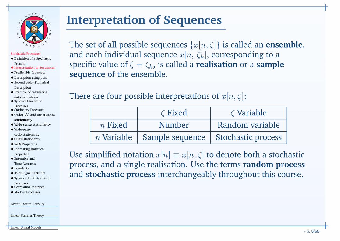
The set of all possible sequences {x[n, ζ]} is called an ensemble,and each individual sequence x[n, ζk], corresponding to aspecific value of ζ = ζk, is called a realisation or a samplesequence of the ensemble.
There are four possible interpretations of x[n, ζ]:
ζ Fixed ζ Variable
n Fixed Number Random variable
n Variable Sample sequence Stochastic process
Use simplified notation x[n] ≡ x[n, ζ] to denote both a stochasticprocess, and a single realisation. Use the terms random processand stochastic process interchangeably throughout this course.

Stochastic Processes
•Definition of a Stochastic
Process• Interpretation of Sequences
•Predictable Processes
•Description using pdfs
•Second-order Statistical
Description
•Example of calculating
autocorrelations•Types of Stochastic
Processes•Stationary Processes
•Order-N and strict-sense
stationarity
•Wide-sense stationarity
•Wide-sense
cyclo-stationarity
•Quasi-stationarity
•WSS Properties
•Estimating statistical
properties
•Ensemble and
Time-Averages
•Ergodicity
• Joint Signal Statistics
•Types of Joint Stochastic
Processes•Correlation Matrices
•Markov Processes
Power Spectral Density
Linear Systems Theory
Linear Signal Models
- p. 6/55
TH
E
UN I V E
RS
IT
Y
OF
ED
I N BU
R
GH
Predictable Processes
The unpredictability of a random process is, in general, thecombined result of the following two characteristics:
1. The selection of a single realisation is based on the outcome ofa random experiment;
2. No functional description is available for all realisations of theensemble.
In some special cases, however, a functional relationship isavailable. This means that after the occurrence of all samples ofa particular realisation up to a particular point, n, all futurevalues can be predicted exactly from the past ones.
If this is the case for a random process, then it is calledpredictable, otherwise it is said to be unpredictable or aregular process.

Stochastic Processes
•Definition of a Stochastic
Process• Interpretation of Sequences
•Predictable Processes
•Description using pdfs
•Second-order Statistical
Description
•Example of calculating
autocorrelations•Types of Stochastic
Processes•Stationary Processes
•Order-N and strict-sense
stationarity
•Wide-sense stationarity
•Wide-sense
cyclo-stationarity
•Quasi-stationarity
•WSS Properties
•Estimating statistical
properties
•Ensemble and
Time-Averages
•Ergodicity
• Joint Signal Statistics
•Types of Joint Stochastic
Processes•Correlation Matrices
•Markov Processes
Power Spectral Density
Linear Systems Theory
Linear Signal Models
- p. 7/55
TH
E
UN I V E
RS
IT
Y
OF
ED
I N BU
R
GH
Description using pdfs
For fixed n = n0, x[n0, ζ] is a random variable. Moreover, therandom vector formed from the k random variables{x[nj ] , j ∈ {1, . . . k}} is characterised by the cumulativedistribution function (cdf) and pdfs:
FX (x1 . . . xk | n1 . . . nk) = Pr (x[n1] ≤ x1, . . . , x[nk] ≤ xk)
fX (x1 . . . xk | n1 . . . nk) =∂kFX (x1 . . . xk | n1 . . . nk)
∂x1 · · · ∂xk

Stochastic Processes
•Definition of a Stochastic
Process• Interpretation of Sequences
•Predictable Processes
•Description using pdfs
•Second-order Statistical
Description
•Example of calculating
autocorrelations•Types of Stochastic
Processes•Stationary Processes
•Order-N and strict-sense
stationarity
•Wide-sense stationarity
•Wide-sense
cyclo-stationarity
•Quasi-stationarity
•WSS Properties
•Estimating statistical
properties
•Ensemble and
Time-Averages
•Ergodicity
• Joint Signal Statistics
•Types of Joint Stochastic
Processes•Correlation Matrices
•Markov Processes
Power Spectral Density
Linear Systems Theory
Linear Signal Models
- p. 7/55
TH
E
UN I V E
RS
IT
Y
OF
ED
I N BU
R
GH
Description using pdfs
For fixed n = n0, x[n0, ζ] is a random variable. Moreover, therandom vector formed from the k random variables{x[nj ] , j ∈ {1, . . . k}} is characterised by the cdf and pdfs:
FX (x1 . . . xk | n1 . . . nk) = Pr (x[n1] ≤ x1, . . . , x[nk] ≤ xk)
fX (x1 . . . xk | n1 . . . nk) =∂kFX (x1 . . . xk | n1 . . . nk)
∂x1 · · · ∂xk
In exactly the same way as with random variables and randomvectors, it is:
difficult to estimate these probability functions withoutconsiderable additional information or assumptions;
possible to frequently characterise stochastic processesusefully with much less information.

Stochastic Processes
•Definition of a Stochastic
Process• Interpretation of Sequences
•Predictable Processes
•Description using pdfs
•Second-order Statistical
Description
•Example of calculating
autocorrelations•Types of Stochastic
Processes•Stationary Processes
•Order-N and strict-sense
stationarity
•Wide-sense stationarity
•Wide-sense
cyclo-stationarity
•Quasi-stationarity
•WSS Properties
•Estimating statistical
properties
•Ensemble and
Time-Averages
•Ergodicity
• Joint Signal Statistics
•Types of Joint Stochastic
Processes•Correlation Matrices
•Markov Processes
Power Spectral Density
Linear Systems Theory
Linear Signal Models
- p. 8/55
TH
E
UN I V E
RS
IT
Y
OF
ED
I N BU
R
GH
Second-order Statistical Description
Mean and Variance Sequence At time n, the ensemble mean andvariance are given by:
µx[n] = E [x[n]]
σ2x[n] = E
[
|x[n]− µx[n] |2]
= E[
|x[n] |2]
− |µx[n] |2
Both µx[n] and σ2x[n] are deterministic sequences.
Autocorrelation sequence The second-order statistic rxx[n1, n2]provides a measure of the dependence between values of theprocess at two different times; it can provide informationabout the time variation of the process:
rxx[n1, n2] = E [x[n1] x∗[n2]]

Stochastic Processes
•Definition of a Stochastic
Process• Interpretation of Sequences
•Predictable Processes
•Description using pdfs
•Second-order Statistical
Description
•Example of calculating
autocorrelations•Types of Stochastic
Processes•Stationary Processes
•Order-N and strict-sense
stationarity
•Wide-sense stationarity
•Wide-sense
cyclo-stationarity
•Quasi-stationarity
•WSS Properties
•Estimating statistical
properties
•Ensemble and
Time-Averages
•Ergodicity
• Joint Signal Statistics
•Types of Joint Stochastic
Processes•Correlation Matrices
•Markov Processes
Power Spectral Density
Linear Systems Theory
Linear Signal Models
- p. 8/55
TH
E
UN I V E
RS
IT
Y
OF
ED
I N BU
R
GH
Second-order Statistical Description
Autocovariance sequence The autocovariance sequence provides ameasure of how similar the deviation from the mean of aprocess is at two different time instances:
γxx[n1, n2] = E [(x[n1]− µx[n1])(x[n2]− µx[n2])∗]
= rxx[n1, n2]− µx[n1] µ∗x[n2]
To show how these deterministic sequences of a stochasticprocess can be calculated, several examples are considered indetail below.

Stochastic Processes
•Definition of a Stochastic
Process• Interpretation of Sequences
•Predictable Processes
•Description using pdfs
•Second-order Statistical
Description
•Example of calculating
autocorrelations•Types of Stochastic
Processes•Stationary Processes
•Order-N and strict-sense
stationarity
•Wide-sense stationarity
•Wide-sense
cyclo-stationarity
•Quasi-stationarity
•WSS Properties
•Estimating statistical
properties
•Ensemble and
Time-Averages
•Ergodicity
• Joint Signal Statistics
•Types of Joint Stochastic
Processes•Correlation Matrices
•Markov Processes
Power Spectral Density
Linear Systems Theory
Linear Signal Models
- p. 9/55
TH
E
UN I V E
RS
IT
Y
OF
ED
I N BU
R
GH
Example of calculating autocorrelations
Example ( [Manolakis:2000, Ex 3.9, page 144]). The harmonic processx[n] is defined by:
x[n] =M∑
k=1
Ak cos(ωkn+ φk), ωk 6= 0
where M , {Ak}M1 and {ωk}M1 are constants, and {φk}M1 arepairwise independent random variables uniformly distributed inthe interval [0, 2π].
1. Determine the mean of x(n).
2. Show the autocorrelation sequence is given by
rxx[ℓ] =1
2
M∑
k=1
|Ak|2 cosωkℓ, −∞ < ℓ < ∞ ⋊⋉

Stochastic Processes
•Definition of a Stochastic
Process• Interpretation of Sequences
•Predictable Processes
•Description using pdfs
•Second-order Statistical
Description
•Example of calculating
autocorrelations•Types of Stochastic
Processes•Stationary Processes
•Order-N and strict-sense
stationarity
•Wide-sense stationarity
•Wide-sense
cyclo-stationarity
•Quasi-stationarity
•WSS Properties
•Estimating statistical
properties
•Ensemble and
Time-Averages
•Ergodicity
• Joint Signal Statistics
•Types of Joint Stochastic
Processes•Correlation Matrices
•Markov Processes
Power Spectral Density
Linear Systems Theory
Linear Signal Models
- p. 9/55
TH
E
UN I V E
RS
IT
Y
OF
ED
I N BU
R
GH
Example of calculating autocorrelations
Example ( [Manolakis:2000, Ex 3.9, page 144]). SOLUTION. 1. Theexpected value of the process is straightforwardly given by:
E [x(n)] = E
[
M∑
k=1
Ak cos(ωkn+ φk)
]
=
M∑
k=1
Ak E [cos(ωkn+ φk)]
Since a co-sinusoid is zero-mean, then:
E [cos(ωkn+ φk)] =
∫ 2π
0
cos(ωkn+ φk)×1
2π× dφk = 0
Hence, it follows:
E [x(n)] = 0, ∀n �

Stochastic Processes
•Definition of a Stochastic
Process• Interpretation of Sequences
•Predictable Processes
•Description using pdfs
•Second-order Statistical
Description
•Example of calculating
autocorrelations•Types of Stochastic
Processes•Stationary Processes
•Order-N and strict-sense
stationarity
•Wide-sense stationarity
•Wide-sense
cyclo-stationarity
•Quasi-stationarity
•WSS Properties
•Estimating statistical
properties
•Ensemble and
Time-Averages
•Ergodicity
• Joint Signal Statistics
•Types of Joint Stochastic
Processes•Correlation Matrices
•Markov Processes
Power Spectral Density
Linear Systems Theory
Linear Signal Models
- p. 9/55
TH
E
UN I V E
RS
IT
Y
OF
ED
I N BU
R
GH
Example of calculating autocorrelations
Example ( [Manolakis:2000, Ex 3.9, page 144]). SOLUTION. 1.
rxx(n1, n2) = E
M∑
k=1
Ak cos(ωkn1 + φk)M∑
j=1
A∗j cos(ωjn2 + φj)
=M∑
k=1
M∑
j=1
Ak A∗jE [cos(ωkn1 + φk) cos(ωjn2 + φj)]
After some algebra, it can be shown that:
E [cos(ωkn1 + φk) cos(ωjn2 + φj)] =
{
12 cosωk(n1 − n2) k = j
0 otherwise
where g(φk) = cos(ωkn1 + φk) and h(φk) = cos(ωjn2 + φj),and the fact that φk and φj are independent implies theexpectation function may be factorised.
E [cos(ω n + φ ) cos(ω n + φ )] =1cosω (n −n ) δ(k− j)

Stochastic Processes
•Definition of a Stochastic
Process• Interpretation of Sequences
•Predictable Processes
•Description using pdfs
•Second-order Statistical
Description
•Example of calculating
autocorrelations•Types of Stochastic
Processes•Stationary Processes
•Order-N and strict-sense
stationarity
•Wide-sense stationarity
•Wide-sense
cyclo-stationarity
•Quasi-stationarity
•WSS Properties
•Estimating statistical
properties
•Ensemble and
Time-Averages
•Ergodicity
• Joint Signal Statistics
•Types of Joint Stochastic
Processes•Correlation Matrices
•Markov Processes
Power Spectral Density
Linear Systems Theory
Linear Signal Models
- p. 10/55
TH
E
UN I V E
RS
IT
Y
OF
ED
I N BU
R
GH
Types of Stochastic Processes
Independence A stochastic process is independent if, and onlyif, (iff)
fX (x1, . . . , xN | n1, . . . , nN ) =N∏
k=1
fXk(xk | nk)
∀N, nk, k ∈ {1, . . . , N}. Here, therefore, x(n) is a sequenceof independent random variables.

Stochastic Processes
•Definition of a Stochastic
Process• Interpretation of Sequences
•Predictable Processes
•Description using pdfs
•Second-order Statistical
Description
•Example of calculating
autocorrelations•Types of Stochastic
Processes•Stationary Processes
•Order-N and strict-sense
stationarity
•Wide-sense stationarity
•Wide-sense
cyclo-stationarity
•Quasi-stationarity
•WSS Properties
•Estimating statistical
properties
•Ensemble and
Time-Averages
•Ergodicity
• Joint Signal Statistics
•Types of Joint Stochastic
Processes•Correlation Matrices
•Markov Processes
Power Spectral Density
Linear Systems Theory
Linear Signal Models
- p. 10/55
TH
E
UN I V E
RS
IT
Y
OF
ED
I N BU
R
GH
Types of Stochastic Processes
Independence A stochastic process is independent iff
fX (x1, . . . , xN | n1, . . . , nN ) =N∏
k=1
fXk(xk | nk)
∀N, nk, k ∈ {1, . . . , N}. Here, therefore, x(n) is a sequenceof independent random variables.
An independent and identically distributed (i. i. d.) proce ss is onewhere all the random variables {x(nk, ζ), nk ∈ Z} have thesame pdf, and x(n) will be called an i. i. d. random process.

Stochastic Processes
•Definition of a Stochastic
Process• Interpretation of Sequences
•Predictable Processes
•Description using pdfs
•Second-order Statistical
Description
•Example of calculating
autocorrelations•Types of Stochastic
Processes•Stationary Processes
•Order-N and strict-sense
stationarity
•Wide-sense stationarity
•Wide-sense
cyclo-stationarity
•Quasi-stationarity
•WSS Properties
•Estimating statistical
properties
•Ensemble and
Time-Averages
•Ergodicity
• Joint Signal Statistics
•Types of Joint Stochastic
Processes•Correlation Matrices
•Markov Processes
Power Spectral Density
Linear Systems Theory
Linear Signal Models
- p. 10/55
TH
E
UN I V E
RS
IT
Y
OF
ED
I N BU
R
GH
Types of Stochastic Processes
Independence A stochastic process is independent iff
fX (x1, . . . , xN | n1, . . . , nN ) =N∏
k=1
fXk(xk | nk)
∀N, nk, k ∈ {1, . . . , N}. Here, therefore, x(n) is a sequenceof independent random variables.
An i. i. d. process is one where all the random variables{x(nk, ζ), nk ∈ Z} have the same pdf, and x(n) will be calledan i. i. d. random process.
An uncorrelated processes is a sequence of uncorrelated randomvariables:
γxx(n1, n2) = σ2x(n1) δ(n1 − n2)

Stochastic Processes
•Definition of a Stochastic
Process• Interpretation of Sequences
•Predictable Processes
•Description using pdfs
•Second-order Statistical
Description
•Example of calculating
autocorrelations•Types of Stochastic
Processes•Stationary Processes
•Order-N and strict-sense
stationarity
•Wide-sense stationarity
•Wide-sense
cyclo-stationarity
•Quasi-stationarity
•WSS Properties
•Estimating statistical
properties
•Ensemble and
Time-Averages
•Ergodicity
• Joint Signal Statistics
•Types of Joint Stochastic
Processes•Correlation Matrices
•Markov Processes
Power Spectral Density
Linear Systems Theory
Linear Signal Models
- p. 10/55
TH
E
UN I V E
RS
IT
Y
OF
ED
I N BU
R
GH
Types of Stochastic Processes
An orthogonal process is a sequence of orthogonal randomvariables, and is given by:
rxx(n1, n2) = E[
|x(n1)|2]
δ(n1 − n2)
If a process is zero-mean, then it is both orthogonal anduncorrelated since γxx(n1, n2) = rxx(n1, n2).
A stationary process is a random process where its statisticalproperties do not vary with time. Processes whose statisticalproperties do change with time are referred to asnonstationary.

Stochastic Processes
•Definition of a Stochastic
Process• Interpretation of Sequences
•Predictable Processes
•Description using pdfs
•Second-order Statistical
Description
•Example of calculating
autocorrelations•Types of Stochastic
Processes•Stationary Processes
•Order-N and strict-sense
stationarity
•Wide-sense stationarity
•Wide-sense
cyclo-stationarity
•Quasi-stationarity
•WSS Properties
•Estimating statistical
properties
•Ensemble and
Time-Averages
•Ergodicity
• Joint Signal Statistics
•Types of Joint Stochastic
Processes•Correlation Matrices
•Markov Processes
Power Spectral Density
Linear Systems Theory
Linear Signal Models
- p. 11/55
TH
E
UN I V E
RS
IT
Y
OF
ED
I N BU
R
GH
Stationary Processes
A random process x(n) has been called stationary if its statisticsdetermined for x(n) are equal to those for x(n+ k), for every k.There are various formal definitions of stationarity, along withquasi-stationary processes, which are discussed below.
Order-N and strict-sense stationarity
Wide-sense stationarity
Wide-sense periodicity and cyclo-stationarity
Local- or quasi-stationary processes
After this, some examples of various stationary processes will begiven.

Stochastic Processes
•Definition of a Stochastic
Process• Interpretation of Sequences
•Predictable Processes
•Description using pdfs
•Second-order Statistical
Description
•Example of calculating
autocorrelations•Types of Stochastic
Processes•Stationary Processes
•Order-N and strict-sense
stationarity
•Wide-sense stationarity
•Wide-sense
cyclo-stationarity
•Quasi-stationarity
•WSS Properties
•Estimating statistical
properties
•Ensemble and
Time-Averages
•Ergodicity
• Joint Signal Statistics
•Types of Joint Stochastic
Processes•Correlation Matrices
•Markov Processes
Power Spectral Density
Linear Systems Theory
Linear Signal Models
- p. 12/55
TH
E
UN I V E
RS
IT
Y
OF
ED
I N BU
R
GH
Order-N and strict-sense stationarity
Definition (Stationary of order- N ). A stochastic process x(n) iscalled stationary of order-N if:
fX (x1, . . . , xN | n1, . . . , nN ) = fX (x1, . . . , xN | n1 + k, . . . , nN + k)♦
for any value of k. If x(n) is stationary for all orders N ∈ Z+, it is
said to be strict-sense stationary (SSS).

Stochastic Processes
•Definition of a Stochastic
Process• Interpretation of Sequences
•Predictable Processes
•Description using pdfs
•Second-order Statistical
Description
•Example of calculating
autocorrelations•Types of Stochastic
Processes•Stationary Processes
•Order-N and strict-sense
stationarity
•Wide-sense stationarity
•Wide-sense
cyclo-stationarity
•Quasi-stationarity
•WSS Properties
•Estimating statistical
properties
•Ensemble and
Time-Averages
•Ergodicity
• Joint Signal Statistics
•Types of Joint Stochastic
Processes•Correlation Matrices
•Markov Processes
Power Spectral Density
Linear Systems Theory
Linear Signal Models
- p. 12/55
TH
E
UN I V E
RS
IT
Y
OF
ED
I N BU
R
GH
Order-N and strict-sense stationarity
Definition (Stationary of order- N ). A stochastic process x(n) iscalled stationary of order-N if:
fX (x1, . . . , xN | n1, . . . , nN ) = fX (x1, . . . , xN | n1 + k, . . . , nN + k)♦
for any value of k. If x(n) is stationary for all orders N ∈ Z+, it is
said to be SSS.
An independent and identically distributed process is SSS since,in this case, fXk
(xk | nk) = fX (xk) is independent of n, andtherefore also of n+ k.
However, SSS is more restrictive than necessary in practicalapplications, and is a rarely required property.

Stochastic Processes
•Definition of a Stochastic
Process• Interpretation of Sequences
•Predictable Processes
•Description using pdfs
•Second-order Statistical
Description
•Example of calculating
autocorrelations•Types of Stochastic
Processes•Stationary Processes
•Order-N and strict-sense
stationarity
•Wide-sense stationarity
•Wide-sense
cyclo-stationarity
•Quasi-stationarity
•WSS Properties
•Estimating statistical
properties
•Ensemble and
Time-Averages
•Ergodicity
• Joint Signal Statistics
•Types of Joint Stochastic
Processes•Correlation Matrices
•Markov Processes
Power Spectral Density
Linear Systems Theory
Linear Signal Models
- p. 13/55
TH
E
UN I V E
RS
IT
Y
OF
ED
I N BU
R
GH
Wide-sense stationarity
A more relaxed form of stationarity, which is sufficient forpractical problems, occurs when a random process is stationaryorder-2; such a process is wide-sense stationary (WSS).

Stochastic Processes
•Definition of a Stochastic
Process• Interpretation of Sequences
•Predictable Processes
•Description using pdfs
•Second-order Statistical
Description
•Example of calculating
autocorrelations•Types of Stochastic
Processes•Stationary Processes
•Order-N and strict-sense
stationarity
•Wide-sense stationarity
•Wide-sense
cyclo-stationarity
•Quasi-stationarity
•WSS Properties
•Estimating statistical
properties
•Ensemble and
Time-Averages
•Ergodicity
• Joint Signal Statistics
•Types of Joint Stochastic
Processes•Correlation Matrices
•Markov Processes
Power Spectral Density
Linear Systems Theory
Linear Signal Models
- p. 13/55
TH
E
UN I V E
RS
IT
Y
OF
ED
I N BU
R
GH
Wide-sense stationarity
Definition (Wide-sense stationarity). A random signal x(n) is calledwide-sense stationary if:
the mean and variance is constant and independent of n:
E [x(n)] = µx
var [x(n)] = σ2x
the autocorrelation depends only on the time differencel = n1 − n2, called the lag:
rxx(n1, n2) = r∗xx(n2, n1) = E [x(n1)x∗(n2)]
= rxx(l) = rxx(n1 − n2) = E [x(n1)x∗(n1 − l)]
= E [x(n2 + l)x∗(n2)]
♦

Stochastic Processes
•Definition of a Stochastic
Process• Interpretation of Sequences
•Predictable Processes
•Description using pdfs
•Second-order Statistical
Description
•Example of calculating
autocorrelations•Types of Stochastic
Processes•Stationary Processes
•Order-N and strict-sense
stationarity
•Wide-sense stationarity
•Wide-sense
cyclo-stationarity
•Quasi-stationarity
•WSS Properties
•Estimating statistical
properties
•Ensemble and
Time-Averages
•Ergodicity
• Joint Signal Statistics
•Types of Joint Stochastic
Processes•Correlation Matrices
•Markov Processes
Power Spectral Density
Linear Systems Theory
Linear Signal Models
- p. 13/55
TH
E
UN I V E
RS
IT
Y
OF
ED
I N BU
R
GH
Wide-sense stationarity
The autocovariance function is given by:
γxx(l) = rxx(l)− |µx|2
Since 2nd-order moments are defined in terms of 2nd-orderpdf, then strict-sense stationary are always WSS, but notnecessarily vice-versa, except if the signal is Gaussian.
In practice, however, it is very rare to encounter a signal thatis stationary in the wide-sense, but not stationary in the strictsense.

Stochastic Processes
•Definition of a Stochastic
Process• Interpretation of Sequences
•Predictable Processes
•Description using pdfs
•Second-order Statistical
Description
•Example of calculating
autocorrelations•Types of Stochastic
Processes•Stationary Processes
•Order-N and strict-sense
stationarity
•Wide-sense stationarity
•Wide-sense
cyclo-stationarity
•Quasi-stationarity
•WSS Properties
•Estimating statistical
properties
•Ensemble and
Time-Averages
•Ergodicity
• Joint Signal Statistics
•Types of Joint Stochastic
Processes•Correlation Matrices
•Markov Processes
Power Spectral Density
Linear Systems Theory
Linear Signal Models
- p. 14/55
TH
E
UN I V E
RS
IT
Y
OF
ED
I N BU
R
GH
Wide-sense cyclo-stationarity
Two classes of nonstationary process which, in part, haveproperties resembling stationary signals are:
1. A wide-sense periodic (WSP) process is classified as signals whosemean is periodic, and whose autocorrelation function isperiodic in both dimensions:
µx(n) = µx(n+N)
rxx(n1, n2) = rxx(n1 +N,n2) = rxx(n1, n2 +N)
= rxx(n1 +N,n2 +N)
for all n, n1 and n2. These are quite tight constraints for realsignals.

Stochastic Processes
•Definition of a Stochastic
Process• Interpretation of Sequences
•Predictable Processes
•Description using pdfs
•Second-order Statistical
Description
•Example of calculating
autocorrelations•Types of Stochastic
Processes•Stationary Processes
•Order-N and strict-sense
stationarity
•Wide-sense stationarity
•Wide-sense
cyclo-stationarity
•Quasi-stationarity
•WSS Properties
•Estimating statistical
properties
•Ensemble and
Time-Averages
•Ergodicity
• Joint Signal Statistics
•Types of Joint Stochastic
Processes•Correlation Matrices
•Markov Processes
Power Spectral Density
Linear Systems Theory
Linear Signal Models
- p. 14/55
TH
E
UN I V E
RS
IT
Y
OF
ED
I N BU
R
GH
Wide-sense cyclo-stationarity
2. A wide-sense cyclo-stationary process has similar but lessrestrictive properties than a WSP process, in that the mean isperiodic, but the autocorrelation function is now justinvariant to a shift by N in both of its arguments:
µx(n) = µx(n+N)
rxx(n1, n2) = rxx(n1 +N,n2 +N)
for all n, n1 and n2. This type of nonstationary process hasmore practical applications, as the following example willshow.

Stochastic Processes
•Definition of a Stochastic
Process• Interpretation of Sequences
•Predictable Processes
•Description using pdfs
•Second-order Statistical
Description
•Example of calculating
autocorrelations•Types of Stochastic
Processes•Stationary Processes
•Order-N and strict-sense
stationarity
•Wide-sense stationarity
•Wide-sense
cyclo-stationarity
•Quasi-stationarity
•WSS Properties
•Estimating statistical
properties
•Ensemble and
Time-Averages
•Ergodicity
• Joint Signal Statistics
•Types of Joint Stochastic
Processes•Correlation Matrices
•Markov Processes
Power Spectral Density
Linear Systems Theory
Linear Signal Models
- p. 15/55
TH
E
UN I V E
RS
IT
Y
OF
ED
I N BU
R
GH
Quasi-stationarity
At the introduction of this lecture course, it was noted that in theanalysis of speech signals, the speech waveform is broken up intoshort segments whose duration is typically 10 to 20 milliseconds.
This is because speech can be modelled as a locally stationaryor quasi-stationary process.
Such processes possess statistical properties that change slowlyover short periods of time.
They are globally nonstationary, but are approximately locallystationary, and are modelled as if the statistics actually arestationary over a short segment of time.

Stochastic Processes
•Definition of a Stochastic
Process• Interpretation of Sequences
•Predictable Processes
•Description using pdfs
•Second-order Statistical
Description
•Example of calculating
autocorrelations•Types of Stochastic
Processes•Stationary Processes
•Order-N and strict-sense
stationarity
•Wide-sense stationarity
•Wide-sense
cyclo-stationarity
•Quasi-stationarity
•WSS Properties
•Estimating statistical
properties
•Ensemble and
Time-Averages
•Ergodicity
• Joint Signal Statistics
•Types of Joint Stochastic
Processes•Correlation Matrices
•Markov Processes
Power Spectral Density
Linear Systems Theory
Linear Signal Models
- p. 16/55
TH
E
UN I V E
RS
IT
Y
OF
ED
I N BU
R
GH
WSS Properties
The average power of a WSS process x(n) satisfies:
rxx(0) = σ2x + |µx|
2
rxx(0) ≥ rxx(l), for all l
The expression for power can be broken down as follows:
Average DC Power: |µx|2
Average AC Power: σ2x
Total average power: rxx(0)
Total average power = Average DC power+Average AC power
Moreover, it follows that γxx(0) ≥ γxx(l).

Stochastic Processes
•Definition of a Stochastic
Process• Interpretation of Sequences
•Predictable Processes
•Description using pdfs
•Second-order Statistical
Description
•Example of calculating
autocorrelations•Types of Stochastic
Processes•Stationary Processes
•Order-N and strict-sense
stationarity
•Wide-sense stationarity
•Wide-sense
cyclo-stationarity
•Quasi-stationarity
•WSS Properties
•Estimating statistical
properties
•Ensemble and
Time-Averages
•Ergodicity
• Joint Signal Statistics
•Types of Joint Stochastic
Processes•Correlation Matrices
•Markov Processes
Power Spectral Density
Linear Systems Theory
Linear Signal Models
- p. 16/55
TH
E
UN I V E
RS
IT
Y
OF
ED
I N BU
R
GH
WSS Properties
It is left as an exercise to show that the autocorrelation sequencerxx(l) is:
a conjugate symmetric function of the lag l:
r∗xx(−l) = rxx(l)
a nonnegative-definite or positive semi-definite function,such that for any sequence α(n):
M∑
n=1
M∑
m=1
α∗(n) rxx(n−m)α(m) ≥ 0
Note that, more generally, even a correlation function for anonstationary random process is positive semi-definite:
M∑
n=1
M∑
m=1
α∗(n) rxx(n,m)α(m) ≥ 0 for any sequence α(n)

Stochastic Processes
•Definition of a Stochastic
Process• Interpretation of Sequences
•Predictable Processes
•Description using pdfs
•Second-order Statistical
Description
•Example of calculating
autocorrelations•Types of Stochastic
Processes•Stationary Processes
•Order-N and strict-sense
stationarity
•Wide-sense stationarity
•Wide-sense
cyclo-stationarity
•Quasi-stationarity
•WSS Properties
•Estimating statistical
properties
•Ensemble and
Time-Averages
•Ergodicity
• Joint Signal Statistics
•Types of Joint Stochastic
Processes•Correlation Matrices
•Markov Processes
Power Spectral Density
Linear Systems Theory
Linear Signal Models
- p. 17/55
TH
E
UN I V E
RS
IT
Y
OF
ED
I N BU
R
GH
Estimating statistical properties
A stochastic process consists of the ensemble, x(n, ζ), and aprobability law, fX ({x} | {n}). If this information is available∀n, the statistical properties are easily determined.
In practice, only a limited number of realisations of a processis available, and often only one: i.e. {x(n, ζk), k ∈ {1, . . . , K}}is known for some K, but fX (x | n) is unknown.
Is is possible to infer the statistical characteristics of a processfrom a single realisation? Yes, for the following class ofsignals:
ergodic processes;
nonstationary processes where additional structure aboutthe autocorrelation function is known (beyond the scope ofthis course).

Stochastic Processes
•Definition of a Stochastic
Process• Interpretation of Sequences
•Predictable Processes
•Description using pdfs
•Second-order Statistical
Description
•Example of calculating
autocorrelations•Types of Stochastic
Processes•Stationary Processes
•Order-N and strict-sense
stationarity
•Wide-sense stationarity
•Wide-sense
cyclo-stationarity
•Quasi-stationarity
•WSS Properties
•Estimating statistical
properties
•Ensemble and
Time-Averages
•Ergodicity
• Joint Signal Statistics
•Types of Joint Stochastic
Processes•Correlation Matrices
•Markov Processes
Power Spectral Density
Linear Systems Theory
Linear Signal Models
- p. 18/55
TH
E
UN I V E
RS
IT
Y
OF
ED
I N BU
R
GH
Ensemble and Time-Averages
Ensemble averaging, as considered so far in the course, is notfrequently used in practice since it is impractical to obtain thenumber of realisations needed for an accurate estimate.
A statistical average that can be obtained from a singlerealisation of a process is a time-average, defined by:
〈g(x(n))〉 , limN→∞
1
2N + 1
N∑
n=−N
g(x(n))
For every ensemble average, a corresponding time-average canbe defined; the above corresponds to: E [g(x(n))].
Time-averages are random variables since they implicitly dependon the particular realisation, given by ζ. Averages ofdeterministic signals are fixed numbers or sequences, eventhough they are given by the same expression.

Stochastic Processes
•Definition of a Stochastic
Process• Interpretation of Sequences
•Predictable Processes
•Description using pdfs
•Second-order Statistical
Description
•Example of calculating
autocorrelations•Types of Stochastic
Processes•Stationary Processes
•Order-N and strict-sense
stationarity
•Wide-sense stationarity
•Wide-sense
cyclo-stationarity
•Quasi-stationarity
•WSS Properties
•Estimating statistical
properties
•Ensemble and
Time-Averages
•Ergodicity
• Joint Signal Statistics
•Types of Joint Stochastic
Processes•Correlation Matrices
•Markov Processes
Power Spectral Density
Linear Systems Theory
Linear Signal Models
- p. 19/55
TH
E
UN I V E
RS
IT
Y
OF
ED
I N BU
R
GH
Ergodicity
A stochastic process, x(n), is ergodic if its ensembleaverages can be estimated from a single realisation of aprocess using time averages.
The two most important degrees of ergodicity are:
Mean-Ergodic (or ergodic in the mean) processes have identicalexpected values and sample-means:
〈x(n)〉 = E [x(n)]
Covariance-Ergodic Processes (or ergodic in correlation) have theproperty that:
〈x(n)x∗(n− l)〉 = E [x(n)x∗(n− l)]

Stochastic Processes
•Definition of a Stochastic
Process• Interpretation of Sequences
•Predictable Processes
•Description using pdfs
•Second-order Statistical
Description
•Example of calculating
autocorrelations•Types of Stochastic
Processes•Stationary Processes
•Order-N and strict-sense
stationarity
•Wide-sense stationarity
•Wide-sense
cyclo-stationarity
•Quasi-stationarity
•WSS Properties
•Estimating statistical
properties
•Ensemble and
Time-Averages
•Ergodicity
• Joint Signal Statistics
•Types of Joint Stochastic
Processes•Correlation Matrices
•Markov Processes
Power Spectral Density
Linear Systems Theory
Linear Signal Models
- p. 19/55
TH
E
UN I V E
RS
IT
Y
OF
ED
I N BU
R
GH
Ergodicity
It should be intuitiveness obvious that ergodic processes mustbe stationary and, moreover, that a process which is ergodicboth in the mean and correlation is WSS.
WSS processes are not necessarily ergodic.
Ergodic is often used to mean both ergodic in the mean andcorrelation.
In practice, only finite records of data are available, andtherefore an estimate of the time-average will be given by
〈g(x(n))〉 =1
N
∑
n∈N
g(x(n))
where N is the number of data-points available. Theperformance of this estimator will be discussed later in thiscourse.

Stochastic Processes
•Definition of a Stochastic
Process• Interpretation of Sequences
•Predictable Processes
•Description using pdfs
•Second-order Statistical
Description
•Example of calculating
autocorrelations•Types of Stochastic
Processes•Stationary Processes
•Order-N and strict-sense
stationarity
•Wide-sense stationarity
•Wide-sense
cyclo-stationarity
•Quasi-stationarity
•WSS Properties
•Estimating statistical
properties
•Ensemble and
Time-Averages
•Ergodicity
• Joint Signal Statistics
•Types of Joint Stochastic
Processes•Correlation Matrices
•Markov Processes
Power Spectral Density
Linear Systems Theory
Linear Signal Models
- p. 20/55
TH
E
UN I V E
RS
IT
Y
OF
ED
I N BU
R
GH
Joint Signal Statistics
Cross-correlation and cross-covariance A measure of thedependence between values of two different stochasticprocesses is given by the cross-correlation andcross-covariance functions:
rxy(n1, n2) = E [x(n1) y∗(n2)]
γxy(n1, n2) = rxy(n1, n2)− µx(n1)µ∗y(n2)
Normalised cross-correlation (or cross-covariance) Thecross-covariance provides a measure of similarity of thedeviation from the respective means of two processes. Itmakes sense to consider this deviation relative to theirstandard deviations; thus, normalised cross-correlations:
ρxy(n1, n2) =γxy(n1, n2)
σx(n1)σy(n2)

Stochastic Processes
•Definition of a Stochastic
Process• Interpretation of Sequences
•Predictable Processes
•Description using pdfs
•Second-order Statistical
Description
•Example of calculating
autocorrelations•Types of Stochastic
Processes•Stationary Processes
•Order-N and strict-sense
stationarity
•Wide-sense stationarity
•Wide-sense
cyclo-stationarity
•Quasi-stationarity
•WSS Properties
•Estimating statistical
properties
•Ensemble and
Time-Averages
•Ergodicity
• Joint Signal Statistics
•Types of Joint Stochastic
Processes•Correlation Matrices
•Markov Processes
Power Spectral Density
Linear Systems Theory
Linear Signal Models
- p. 21/55
TH
E
UN I V E
RS
IT
Y
OF
ED
I N BU
R
GH
Types of Joint Stochastic Processes
Statistically independence of two stochastic processes occurs when,for every nx and ny,
fXY (x, y | nx, ny) = fX (x | nx) fY (y | ny)
Uncorrelated stochastic processes have, for all nx & ny 6= nx:
γxy(nx, ny) = 0
rxy(nx, ny) = µx(nx)µy(ny)
Joint stochastic processes that are statistically independent areuncorrelated, but not necessarily vice-versa, except for Gaussianprocesses. Nevertheless, a measure of uncorrelatedness is oftenused as a measure of independence. More on this later.

Stochastic Processes
•Definition of a Stochastic
Process• Interpretation of Sequences
•Predictable Processes
•Description using pdfs
•Second-order Statistical
Description
•Example of calculating
autocorrelations•Types of Stochastic
Processes•Stationary Processes
•Order-N and strict-sense
stationarity
•Wide-sense stationarity
•Wide-sense
cyclo-stationarity
•Quasi-stationarity
•WSS Properties
•Estimating statistical
properties
•Ensemble and
Time-Averages
•Ergodicity
• Joint Signal Statistics
•Types of Joint Stochastic
Processes•Correlation Matrices
•Markov Processes
Power Spectral Density
Linear Systems Theory
Linear Signal Models
- p. 21/55
TH
E
UN I V E
RS
IT
Y
OF
ED
I N BU
R
GH
Types of Joint Stochastic Processes
Orthogonal joint processes have, for every n1 and n2 6= n1:
rxy(n1, n2) = 0
Joint WSS is a similar to WSS for a single stochastic process, andis useful since it facilitates a spectral description, as discussedlater in this course:
rxy(l) = rxy(n1 − n2) = r∗yx(−l) = E [x(n) y∗(n− l)]
γxy(l) = γxy(n1 − n2) = γ∗yx(−l) = rxy(l)− µx µ
∗y
Joint-Ergodicity applies to two ergodic processes, x(n) and y(n),whose ensemble cross-correlation can be estimated from atime-average:
〈x(n) y∗(n− l)〉 = E [x(n) y∗(n− l)]

Stochastic Processes
•Definition of a Stochastic
Process• Interpretation of Sequences
•Predictable Processes
•Description using pdfs
•Second-order Statistical
Description
•Example of calculating
autocorrelations•Types of Stochastic
Processes•Stationary Processes
•Order-N and strict-sense
stationarity
•Wide-sense stationarity
•Wide-sense
cyclo-stationarity
•Quasi-stationarity
•WSS Properties
•Estimating statistical
properties
•Ensemble and
Time-Averages
•Ergodicity
• Joint Signal Statistics
•Types of Joint Stochastic
Processes•Correlation Matrices
•Markov Processes
Power Spectral Density
Linear Systems Theory
Linear Signal Models
- p. 22/55
TH
E
UN I V E
RS
IT
Y
OF
ED
I N BU
R
GH
Correlation Matrices
Let an M -dimensional random vector X(n, ζ) ≡ X(n) be derivedfrom the random process x(n) as follows:
X(n) ,[
x(n) x(n− 1) · · · x(n−M + 1)]T
Then its mean is given by an M -vector
µX(n) ,
[
µx(n) µx(n− 1) · · · µx(n−M + 1)]T
and the M ×M correlation matrix is given by:
RX(n) ,
rxx(n, n) · · · rxx(n, n−M + 1)...
. . ....
rxx(n−M + 1, n) · · · rxx(n−M + 1, n−M + 1)

Stochastic Processes
•Definition of a Stochastic
Process• Interpretation of Sequences
•Predictable Processes
•Description using pdfs
•Second-order Statistical
Description
•Example of calculating
autocorrelations•Types of Stochastic
Processes•Stationary Processes
•Order-N and strict-sense
stationarity
•Wide-sense stationarity
•Wide-sense
cyclo-stationarity
•Quasi-stationarity
•WSS Properties
•Estimating statistical
properties
•Ensemble and
Time-Averages
•Ergodicity
• Joint Signal Statistics
•Types of Joint Stochastic
Processes•Correlation Matrices
•Markov Processes
Power Spectral Density
Linear Systems Theory
Linear Signal Models
- p. 22/55
TH
E
UN I V E
RS
IT
Y
OF
ED
I N BU
R
GH
Correlation Matrices
For stationary processes, the correlation matrix has an interestingadditional structure. Note that:
1. RX(n) is a constant matrix RX;
2. rxx(n− i, n− j) = rxx(j − i) = rxx(l), l = j − i;
3. conjugate symmetry gives rxx(l) = r∗xx(−l).
Hence, the matrix Rxx is given by:
RX ,
rxx(0) rxx(1) rxx(2) · · · rxx(M − 1)
r∗xx(1) rxx(0) rxx(1) · · · rxx(M − 2)
r∗xx(2) r∗xx(1) rxx(0) · · · rxx(M − 3)...
......
. . ....
r∗xx(M − 1) r∗xx(M − 2) r∗xx(M − 3) · · · rxx(0)

Stochastic Processes
•Definition of a Stochastic
Process• Interpretation of Sequences
•Predictable Processes
•Description using pdfs
•Second-order Statistical
Description
•Example of calculating
autocorrelations•Types of Stochastic
Processes•Stationary Processes
•Order-N and strict-sense
stationarity
•Wide-sense stationarity
•Wide-sense
cyclo-stationarity
•Quasi-stationarity
•WSS Properties
•Estimating statistical
properties
•Ensemble and
Time-Averages
•Ergodicity
• Joint Signal Statistics
•Types of Joint Stochastic
Processes•Correlation Matrices
•Markov Processes
Power Spectral Density
Linear Systems Theory
Linear Signal Models
- p. 23/55
TH
E
UN I V E
RS
IT
Y
OF
ED
I N BU
R
GH
Markov Processes
A powerful model for a stochastic process known as a Markovmodel is introduced; such a process that satisfies this model isknown as a Markov process.
Quite simply, a Markov process is one in which the probability ofany particular value in a sequence is dependent upon thepreceding sample values.
The simplest kind of dependence arises when the probability ofany sample depends only upon the value of the immediatelypreceding sample, and this is known as a first-order Markovprocess.
This simple process is a surprisingly good model for a number ofpractical signal processing, communications and controlproblems.

Stochastic Processes
•Definition of a Stochastic
Process• Interpretation of Sequences
•Predictable Processes
•Description using pdfs
•Second-order Statistical
Description
•Example of calculating
autocorrelations•Types of Stochastic
Processes•Stationary Processes
•Order-N and strict-sense
stationarity
•Wide-sense stationarity
•Wide-sense
cyclo-stationarity
•Quasi-stationarity
•WSS Properties
•Estimating statistical
properties
•Ensemble and
Time-Averages
•Ergodicity
• Joint Signal Statistics
•Types of Joint Stochastic
Processes•Correlation Matrices
•Markov Processes
Power Spectral Density
Linear Systems Theory
Linear Signal Models
- p. 23/55
TH
E
UN I V E
RS
IT
Y
OF
ED
I N BU
R
GH
Markov Processes
As an example of a Markov process, consider the processgenerated by the difference equation
x(n) = −a x(n− 1) + w(n)
where a is a known constant, and w(n) is a sequence of
zero-mean i. i. d. Gaussian random variables with variance σ2W
density:
fW (w(n)) =1
√
2πσ2W
exp
{
−w(n)2
2σ2W
}
The conditional density of x(n) given x(n− 1) is also Gaussian,
fX (x(n) | x(n− 1)) =1
√
2πσ2W
exp
{
−(x(n) + ax(n− 1))2
2σ2W
}

Stochastic Processes
•Definition of a Stochastic
Process• Interpretation of Sequences
•Predictable Processes
•Description using pdfs
•Second-order Statistical
Description
•Example of calculating
autocorrelations•Types of Stochastic
Processes•Stationary Processes
•Order-N and strict-sense
stationarity
•Wide-sense stationarity
•Wide-sense
cyclo-stationarity
•Quasi-stationarity
•WSS Properties
•Estimating statistical
properties
•Ensemble and
Time-Averages
•Ergodicity
• Joint Signal Statistics
•Types of Joint Stochastic
Processes•Correlation Matrices
•Markov Processes
Power Spectral Density
Linear Systems Theory
Linear Signal Models
- p. 23/55
TH
E
UN I V E
RS
IT
Y
OF
ED
I N BU
R
GH
Markov Processes
Definition (Markov Process). A random process is a P th-orderMarkov process if the distribution of x(n), given the infinite past,depends only on the previous P samples{x(n− 1), . . . , x(n− P )}; that is, if:
fX (x(n) | x(n− 1), x(n− 2), . . . ) = fX (x(n) | x(n− 1), . . . , x(n− P ))♦
Finally, it is noted that if x(n) takes on a countable (discrete) setof values, a Markov random process is called a Markov chain.
- p. 24/55
Handout 3Power Spectral Density

Stochastic Processes
Power Spectral Density
• Introduction
•The power spectral
density
•Properties of the power
spectral density
•General form of the PSD
•The cross-power spectral
density
•Complex Spectral Density
Functions
Linear Systems Theory
Linear Signal Models
- p. 25/55
TH
E
UN I V E
RS
IT
Y
OF
ED
I N BU
R
GH
Introduction
Frequency- and transform-domain methods are very powerfultools for the analysis of deterministic sequences. It seems naturalto extend these techniques to analysis stationary randomprocesses.
So far in this course, stationary stochastic processes have beenconsidered in the time-domain through the use of theautocorrelation function (ACF).

Stochastic Processes
Power Spectral Density
• Introduction
•The power spectral
density
•Properties of the power
spectral density
•General form of the PSD
•The cross-power spectral
density
•Complex Spectral Density
Functions
Linear Systems Theory
Linear Signal Models
- p. 25/55
TH
E
UN I V E
RS
IT
Y
OF
ED
I N BU
R
GH
Introduction
Frequency- and transform-domain methods are very powerfultools for the analysis of deterministic sequences. It seems naturalto extend these techniques to analysis stationary randomprocesses.
So far in this course, stationary stochastic processes have beenconsidered in the time-domain through the use of the ACF.
Since the ACF for a stationary process is a function of asingle-discrete time process, then the question arises as to whatthe discrete-time Fourier transform (DTFT) corresponds to.

Stochastic Processes
Power Spectral Density
• Introduction
•The power spectral
density
•Properties of the power
spectral density
•General form of the PSD
•The cross-power spectral
density
•Complex Spectral Density
Functions
Linear Systems Theory
Linear Signal Models
- p. 25/55
TH
E
UN I V E
RS
IT
Y
OF
ED
I N BU
R
GH
Introduction
Frequency- and transform-domain methods are very powerfultools for the analysis of deterministic sequences. It seems naturalto extend these techniques to analysis stationary randomprocesses.
So far in this course, stationary stochastic processes have beenconsidered in the time-domain through the use of the ACF.
Since the ACF for a stationary process is a function of asingle-discrete time process, then the question arises as to whatthe DTFT corresponds to.
It turns out to be known as the power spectral density (PSD) ofa stationary random process, and the PSD is an extremelypowerful and conceptually appealing tool in statistical signalprocessing.

Stochastic Processes
Power Spectral Density
• Introduction
•The power spectral
density
•Properties of the power
spectral density
•General form of the PSD
•The cross-power spectral
density
•Complex Spectral Density
Functions
Linear Systems Theory
Linear Signal Models
- p. 25/55
TH
E
UN I V E
RS
IT
Y
OF
ED
I N BU
R
GH
Introduction
In signal theory for deterministic signals, spectra are used torepresent a function as a superposition of exponential functions.

Stochastic Processes
Power Spectral Density
• Introduction
•The power spectral
density
•Properties of the power
spectral density
•General form of the PSD
•The cross-power spectral
density
•Complex Spectral Density
Functions
Linear Systems Theory
Linear Signal Models
- p. 25/55
TH
E
UN I V E
RS
IT
Y
OF
ED
I N BU
R
GH
Introduction
In signal theory for deterministic signals, spectra are used torepresent a function as a superposition of exponential functions.For random signals, the notion of a spectrum has twointerpretations:
Transform of averages The first involves transform of averages (ormoments). As will be seen, this will be the Fourier transformof the autocorrelation function.
Stochastic decomposition The second interpretation represents astochastic process as a superposition of exponentials, wherethe coefficients are themselves random variables. Hence, x(n)can be represented as:
x(n) =1
2π
∫ π
−π
X(ejω) ejωn dω, n ∈ R
where X(ejω) is a random variable for a given value of ω.

Stochastic Processes
Power Spectral Density
• Introduction
•The power spectral
density
•Properties of the power
spectral density
•General form of the PSD
•The cross-power spectral
density
•Complex Spectral Density
Functions
Linear Systems Theory
Linear Signal Models
- p. 26/55
TH
E
UN I V E
RS
IT
Y
OF
ED
I N BU
R
GH
The power spectral density
The discrete-time Fourier transform of the autocorrelationfunction of a stationary stochastic process x[n, ζ] is known as the
power spectral density (PSD), is denoted by Pxx(ejω), and is
given by:
Pxx(ejω) =
∑
ℓ∈Z
rxx[ℓ] e−jωℓ
where ω is frequency in radians per sample.
The autocorrelation function, rxx[ℓ], can be recovered from thePSD by using the inverse-DTFT:
rxx[ℓ] =1
2π
∫ π
−π
Pxx(ejω) ejωℓ dω, ℓ ∈ Z

Stochastic Processes
Power Spectral Density
• Introduction
•The power spectral
density
•Properties of the power
spectral density
•General form of the PSD
•The cross-power spectral
density
•Complex Spectral Density
Functions
Linear Systems Theory
Linear Signal Models
- p. 27/55
TH
E
UN I V E
RS
IT
Y
OF
ED
I N BU
R
GH
Properties of the power spectral density
Pxx(ejω) : ω → R
+; in otherwords, the PSD is real valued, andnonnegative definite. i.e.
Pxx(ejω) ≥ 0
Pxx(ejω) = Pxx(e
j(ω+2nπ)); in otherwords, the PSD is periodicwith period 2π.
If x[n] is real-valued, then:
rxx[ℓ] is real and even;
Pxx(ejω) = Pxx(e
−jω) is an even function of ω.
The area under Pxx(ejω) is nonnegative and is equal to the
average power of x[n]. Hence:
1
2π
∫ π
−π
Pxx(ejω) dω = rxx[0] = E
[
|x[n] |2]
≥ 0

Stochastic Processes
Power Spectral Density
• Introduction
•The power spectral
density
•Properties of the power
spectral density
•General form of the PSD
•The cross-power spectral
density
•Complex Spectral Density
Functions
Linear Systems Theory
Linear Signal Models
- p. 28/55
TH
E
UN I V E
RS
IT
Y
OF
ED
I N BU
R
GH
General form of the PSD
A process, x(n), and therefore its corresponding autocorrelationfunction (ACF), rxx(l), can always be decomposed into a
zero-mean aperiodic component, r(a)xx (l), and a non-zero-mean
periodic component, r(p)xx (l):
rxx(l) = r(a)xx (l) + r(p)xx (l)
Theorem (PSD of a non-zero-mean process with periodic compo nent).The most general definition of the PSD for a non-zero-meanstochastic process with a periodic component is
Pxx(ejω) = P (a)
xx (ejω) +2π
K
∑
k∈K
P (p)xx (k) δ (ω − ωk) ♦
P(a)xx (ejω) is the DTFT of r
(a)xx (l), while P
(p)xx (k) are the discrete
Fourier transform (DFT) coefficients for r(p)xx (l) .

Stochastic Processes
Power Spectral Density
• Introduction
•The power spectral
density
•Properties of the power
spectral density
•General form of the PSD
•The cross-power spectral
density
•Complex Spectral Density
Functions
Linear Systems Theory
Linear Signal Models
- p. 28/55
TH
E
UN I V E
RS
IT
Y
OF
ED
I N BU
R
GH
General form of the PSD
Example ( [Manolakis:2001, Harmonic Processes, Page 110-1 11]).Determine the PSD of the harmonic process defined by:
x[n] =
M∑
k=1
Ak cos(ωkn+ φk), ωk 6= 0
⋊⋉

Stochastic Processes
Power Spectral Density
• Introduction
•The power spectral
density
•Properties of the power
spectral density
•General form of the PSD
•The cross-power spectral
density
•Complex Spectral Density
Functions
Linear Systems Theory
Linear Signal Models
- p. 28/55
TH
E
UN I V E
RS
IT
Y
OF
ED
I N BU
R
GH
General form of the PSD
Example ( [Manolakis:2001, Harmonic Processes, Page 110-1 11]).Determine the PSD of the harmonic process defined by:
x[n] =
M∑
k=1
Ak cos(ωkn+ φk), ωk 6= 0
SOLUTION. x[n] is a stationary process with zero-mean, andautocorrelation function (ACF):
rxx[ℓ] =1
2
M∑
k=1
|Ak|2 cosωkℓ, −∞ < ℓ < ∞
�

Stochastic Processes
Power Spectral Density
• Introduction
•The power spectral
density
•Properties of the power
spectral density
•General form of the PSD
•The cross-power spectral
density
•Complex Spectral Density
Functions
Linear Systems Theory
Linear Signal Models
- p. 28/55
TH
E
UN I V E
RS
IT
Y
OF
ED
I N BU
R
GH
General form of the PSD
Example ( [Manolakis:2001, Harmonic Processes, Page 110-1 11]).Determine the PSD of the harmonic process defined by:
x[n] =
M∑
k=1
Ak cos(ωkn+ φk), ωk 6= 0
SOLUTION. Hence, the ACF can be written as:
rxx[ℓ] =M∑
k=−M
|Ak|2
4ejωkℓ, −∞ < ℓ < ∞ �
where the following are defined: A0 = 0, Ak = A−k, andω−k = −ωk.

Stochastic Processes
Power Spectral Density
• Introduction
•The power spectral
density
•Properties of the power
spectral density
•General form of the PSD
•The cross-power spectral
density
•Complex Spectral Density
Functions
Linear Systems Theory
Linear Signal Models
- p. 28/55
TH
E
UN I V E
RS
IT
Y
OF
ED
I N BU
R
GH
General form of the PSD
Example ( [Manolakis:2001, Harmonic Processes, Page 110-1 11]).Determine the PSD of the harmonic process defined by:
x[n] =
M∑
k=1
Ak cos(ωkn+ φk), ωk 6= 0
SOLUTION. Hence, the ACF can be written as:
rxx[ℓ] =M∑
k=−M
|Ak|2
4ejωkℓ, −∞ < ℓ < ∞
where the following are defined: A0 = 0, Ak = A−k, andω−k = −ωk.
Hence, it directly follows
Pxx(ejω) = 2π
M∑
k=−M
|Ak|2
4δ(ω−ωk) =
π
2
M∑
k=−M
|Ak|2δ(ω−ωk) �

Stochastic Processes
Power Spectral Density
• Introduction
•The power spectral
density
•Properties of the power
spectral density
•General form of the PSD
•The cross-power spectral
density
•Complex Spectral Density
Functions
Linear Systems Theory
Linear Signal Models
- p. 29/55
TH
E
UN I V E
RS
IT
Y
OF
ED
I N BU
R
GH
The cross-power spectral density
The cross-power spectral density (CPSD) of two jointly stationarystochastic processes, x(n) and y(n), provides a description oftheir statistical relations in the frequency domain.
It is defined, naturally, as the DTFT of the cross-correlation,
rxy(ℓ) , E [x(n) y∗(n− ℓ)]:
Pxy(ejω) = F{rxy(ℓ)} =
∑
l∈Z
rxy(ℓ) e−jωℓ
The cross-correlation rxy(l) can be recovered by using the
inverse-DTFT:
rxy(l) =1
2π
∫ π
−π
Pxy(ejω) ejωl dω, l ∈ R
The cross-spectrum Pxy(ejω) is, in general, a complex function of
ω.

Stochastic Processes
Power Spectral Density
• Introduction
•The power spectral
density
•Properties of the power
spectral density
•General form of the PSD
•The cross-power spectral
density
•Complex Spectral Density
Functions
Linear Systems Theory
Linear Signal Models
- p. 29/55
TH
E
UN I V E
RS
IT
Y
OF
ED
I N BU
R
GH
The cross-power spectral density
Some properties of the CPSD and related definitions include:
1. Pxy(ejω) is periodic in ω with period 2π.
2. Since rxy(l) = r∗yx(−l), then it follows:
Pxy(ejω) = P ∗
yx(ejω)
3. If the process x(n) is real, then rxy(l) is real, and:
Pxy(ejω) = P ∗
xy(e−jω)
4. The coherence function, is given by:
Γxy(ejω) ,
Pxy(ejω)
√
Pxx(ejω)√
Pyy(ejω)

Stochastic Processes
Power Spectral Density
• Introduction
•The power spectral
density
•Properties of the power
spectral density
•General form of the PSD
•The cross-power spectral
density
•Complex Spectral Density
Functions
Linear Systems Theory
Linear Signal Models
- p. 30/55
TH
E
UN I V E
RS
IT
Y
OF
ED
I N BU
R
GH
Complex Spectral Density Functions
The second moment quantities that described a random processin the transform domain are known as the complex spectraldensity and complex cross-spectral density functions.
Hence, rxx(l)z⇋ Pxx(z) and rxy(l)
z⇋ Pxy(z), where:
Pxx(z) =∑
l∈Z
rxx(l) z−l
Pxy(z) =∑
l∈Z
rxy(l) z−l
If the unit circle, defined by z = ejω is within the region ofconvergence of these summations, then:
Pxx(ejω) = Pxx(z)|z=ejω
Pxy(ejω) = Pxy(z)|z=ejω

Stochastic Processes
Power Spectral Density
• Introduction
•The power spectral
density
•Properties of the power
spectral density
•General form of the PSD
•The cross-power spectral
density
•Complex Spectral Density
Functions
Linear Systems Theory
Linear Signal Models
- p. 30/55
TH
E
UN I V E
RS
IT
Y
OF
ED
I N BU
R
GH
Complex Spectral Density Functions
The inverse of the complex spectral and cross-spectral densitiesare given by the contour integral:
rxx(l) =1
2πj
∮
C
Pxx(z) zl−1 dz
rxy(l) =1
2πj
∮
C
Pxy(z) zl−1 dz
Some properties of the complex spectral densities include:
1. Conjugate-symmetry:
Pxx(z) = P ∗xx(1/z
∗) and Pxy(z) = P ∗xy(1/z
∗)
2. For the case when x(n) is real, then:
Pxx(z) = Pxx(z−1)

- p. 31/55
Handout 4Linear Systems Theory

Stochastic Processes
Power Spectral Density
Linear Systems Theory
•Systems with Stochastic
Inputs
•LTI Systems with
Stationary Inputs
• Input-output Statistics of a
linear time-invariant (LTI)
System
•System identification
•LTV Systems with
Nonstationary Inputs
•Difference Equation
•Frequency-Domain
Analysis of LTI systems
Linear Signal Models
- p. 32/55
TH
E
UN I V E
RS
IT
Y
OF
ED
I N BU
R
GH
Systems with Stochastic Inputs
A graphical representation of a random process at theoutput of a system in relation to a random process at the
input of the system.
What does it mean to apply a stochastic signal to the input of asystem?

Stochastic Processes
Power Spectral Density
Linear Systems Theory
•Systems with Stochastic
Inputs
•LTI Systems with
Stationary Inputs
• Input-output Statistics of a
LTI System
•System identification
•LTV Systems with
Nonstationary Inputs
•Difference Equation
•Frequency-Domain
Analysis of LTI systems
Linear Signal Models
- p. 32/55
TH
E
UN I V E
RS
IT
Y
OF
ED
I N BU
R
GH
Systems with Stochastic Inputs
In principle, the statistics of the output of a system can beexpressed in terms of the statistics of the input. However, ingeneral this is a complicated problem except in special cases.
A special case is that of linear systems, and this is considerednext.

Stochastic Processes
Power Spectral Density
Linear Systems Theory
•Systems with Stochastic
Inputs
•LTI Systems with
Stationary Inputs
• Input-output Statistics of a
LTI System
•System identification
•LTV Systems with
Nonstationary Inputs
•Difference Equation
•Frequency-Domain
Analysis of LTI systems
Linear Signal Models
- p. 33/55
TH
E
UN I V E
RS
IT
Y
OF
ED
I N BU
R
GH
LTI Systems with Stationary Inputs
Since each sequence (realisation) of a stochastic process is adeterministic signal, there is a well-defined input signalproducing a well-defined output signal corresponding to a singlerealisation of the output stochastic process:
y(n, ζ) =∞∑
k=−∞
h(k)x(n− k, ζ)
A complete description of y(n, ζ) requires the computation ofan infinite number of convolutions, corresponding to eachvalue of ζ.
Thus, a better description would be to consider the statisticalproperties of y(n, ζ) in terms of the statistical properties of theinput and the characteristics of the system.

Stochastic Processes
Power Spectral Density
Linear Systems Theory
•Systems with Stochastic
Inputs
•LTI Systems with
Stationary Inputs
• Input-output Statistics of a
LTI System
•System identification
•LTV Systems with
Nonstationary Inputs
•Difference Equation
•Frequency-Domain
Analysis of LTI systems
Linear Signal Models
- p. 33/55
TH
E
UN I V E
RS
IT
Y
OF
ED
I N BU
R
GH
LTI Systems with Stationary Inputs
To investigate the statistical input-output properties of a linearsystem, note the following fundamental theorem:
Theorem (Expectation in Linear Systems). For any linear system,
E [L[x(n)]] = L[E [x(n)]]
In other words, the mean µy(n) of the output y(n) equals theresponse of the system to the mean µx(n) of the input:
µy(n) = L[µx(n)] ♦

Stochastic Processes
Power Spectral Density
Linear Systems Theory
•Systems with Stochastic
Inputs
•LTI Systems with
Stationary Inputs
• Input-output Statistics of a
LTI System
•System identification
•LTV Systems with
Nonstationary Inputs
•Difference Equation
•Frequency-Domain
Analysis of LTI systems
Linear Signal Models
- p. 34/55
TH
E
UN I V E
RS
IT
Y
OF
ED
I N BU
R
GH
Input-output Statistics of a LTI System
If a stationary stochastic process x[n] with mean value µx andcorrelation rxx[ℓ] is applied to the input of a LTI system with
impulse response h[n] and transfer function H(ejω), then the:
Output mean value is given by:
µy = µx
∞∑
k=−∞
h[k] = µx H(ej0)
Input-output cross-correlation is given by:
rxy[ℓ] = h∗[−ℓ] ∗ rxx[ℓ] =∞∑
k=−∞
h∗[−k] rxx[ℓ− k]
Similarly, it follows that ryx(l) = h(l) ∗ rxx(l).

Stochastic Processes
Power Spectral Density
Linear Systems Theory
•Systems with Stochastic
Inputs
•LTI Systems with
Stationary Inputs
• Input-output Statistics of a
LTI System
•System identification
•LTV Systems with
Nonstationary Inputs
•Difference Equation
•Frequency-Domain
Analysis of LTI systems
Linear Signal Models
- p. 34/55
TH
E
UN I V E
RS
IT
Y
OF
ED
I N BU
R
GH
Input-output Statistics of a LTI System
Output autocorrelation is obtained by pre-multiplying thesystem-output by y∗(n− l) and taking expectations:
ryy(l) =∞∑
k=−∞
h(k)E [x(n− k) y∗(n− l)] = h(l) ∗ rxy(l)
Substituting the expression for rxy(l) gives:
ryy(l) = h(l) ∗ h∗(−l) ∗ rxx(l) = rhh(l) ∗ rxx(l)
An equivalent LTI system for autocorrelation filtration.

Stochastic Processes
Power Spectral Density
Linear Systems Theory
•Systems with Stochastic
Inputs
•LTI Systems with
Stationary Inputs
• Input-output Statistics of a
LTI System
•System identification
•LTV Systems with
Nonstationary Inputs
•Difference Equation
•Frequency-Domain
Analysis of LTI systems
Linear Signal Models
- p. 34/55
TH
E
UN I V E
RS
IT
Y
OF
ED
I N BU
R
GH
Input-output Statistics of a LTI System
Output-power of the process y(n) is given by ryy(0) = E[
|y(n)|2]
,
and therefore since ryy(l) = rhh(l) ∗ rxx(l),
Noting power, Pyy, is real, then taking complex-conjugates usingr∗xx(−l) = rxx(l):
Pyy =∑∞
k=−∞ r∗hh(k) rxx(k) =∑∞
n=−∞h∗(n)
∑∞
k=−∞rxx(n+ k)h(k)
Output pdf In general, it is very difficult to calculate the pdf of theoutput of a LTI system, except in special cases, namelyGaussian processes.

Stochastic Processes
Power Spectral Density
Linear Systems Theory
•Systems with Stochastic
Inputs
•LTI Systems with
Stationary Inputs
• Input-output Statistics of a
LTI System
•System identification
•LTV Systems with
Nonstationary Inputs
•Difference Equation
•Frequency-Domain
Analysis of LTI systems
Linear Signal Models
- p. 35/55
TH
E
UN I V E
RS
IT
Y
OF
ED
I N BU
R
GH
System identification
System identification by cross-correlation.
The system is excited with a white Gaussian noise (WGN) inputwith autocorrelation function:
rxx(l) = δ(l)
Since the output-input cross-correlation can be written as:
ryx(l) = h(l) ∗ rxx(l)
then, with rxx(l) = δ(l), it follows:
ryx(l) = h(l) ∗ δ(l) = h(l)

Stochastic Processes
Power Spectral Density
Linear Systems Theory
•Systems with Stochastic
Inputs
•LTI Systems with
Stationary Inputs
• Input-output Statistics of a
LTI System
•System identification
•LTV Systems with
Nonstationary Inputs
•Difference Equation
•Frequency-Domain
Analysis of LTI systems
Linear Signal Models
- p. 36/55
TH
E
UN I V E
RS
IT
Y
OF
ED
I N BU
R
GH
LTV Systems with Nonstationary Inputs
General LTV system with nonstationary input
The input and output are related by the generalised convolution:
y(n) =∞∑
k=−∞
h(n, k)x(k)
where h(n, k) is the response at time-index n to an impulseoccurring at the system input at time-index k.
The mean, autocorrelation and autocovariance sequences of theoutput, y(n), as well as the cross-correlation and cross-covariancefunctions between the input and the output, can be calculated ina similar way as for LTI systems with stationary inputs.

Stochastic Processes
Power Spectral Density
Linear Systems Theory
•Systems with Stochastic
Inputs
•LTI Systems with
Stationary Inputs
• Input-output Statistics of a
LTI System
•System identification
•LTV Systems with
Nonstationary Inputs
•Difference Equation
•Frequency-Domain
Analysis of LTI systems
Linear Signal Models
- p. 37/55
TH
E
UN I V E
RS
IT
Y
OF
ED
I N BU
R
GH
Difference Equation
Consider a LTI system that can be represented by a differenceequation:
P∑
p=0
ap y(n− p) =
Q∑
q=0
bq x(n− q)
where a0 , 1.
Assuming that both x(n) and y(n) are stationary processes, thentaking expectations of both sides gives,
µy =
∑Q
q=0 bq
1 +∑P
p=1 apµx

Stochastic Processes
Power Spectral Density
Linear Systems Theory
•Systems with Stochastic
Inputs
•LTI Systems with
Stationary Inputs
• Input-output Statistics of a
LTI System
•System identification
•LTV Systems with
Nonstationary Inputs
•Difference Equation
•Frequency-Domain
Analysis of LTI systems
Linear Signal Models
- p. 37/55
TH
E
UN I V E
RS
IT
Y
OF
ED
I N BU
R
GH
Difference Equation
Next, multiplying the system equation throughout by y∗(m) andtaking expectations gives:
P∑
p=0
ap ryy(n− p,m) =
Q∑
q=0
bq rxy(n− q,m)
Similarly, instead multiply though by x∗(m) to give:
P∑
p=0
ap ryx(n− p,m) =
Q∑
q=0
bq rxx(n− q,m)
These two difference equations may be used to solve forryy(n1, n2) and rxy(n1, n2). Similar expressions can be obtainedfor the covariance functions.

Stochastic Processes
Power Spectral Density
Linear Systems Theory
•Systems with Stochastic
Inputs
•LTI Systems with
Stationary Inputs
• Input-output Statistics of a
LTI System
•System identification
•LTV Systems with
Nonstationary Inputs
•Difference Equation
•Frequency-Domain
Analysis of LTI systems
Linear Signal Models
- p. 37/55
TH
E
UN I V E
RS
IT
Y
OF
ED
I N BU
R
GH
Difference Equation
Example ( [Manolakis:2000, Example 3.6.2, Page 141]). Let x(n) be arandom process generated by the first order difference equationgiven by:
x(n) = αx(n− 1) + w(n), |α| ≤ 1, n ∈ Z ⋊⋉
where w(n) ∼ N(
µw, σ2w
)
is an i. i. d. WGN process.
Demonstrate that the process x(n) is stationary, anddetermine the mean µx.
Determine the autocovariance and autocorrelation function,γxx(l) and rxx(l).

Stochastic Processes
Power Spectral Density
Linear Systems Theory
•Systems with Stochastic
Inputs
•LTI Systems with
Stationary Inputs
• Input-output Statistics of a
LTI System
•System identification
•LTV Systems with
Nonstationary Inputs
•Difference Equation
•Frequency-Domain
Analysis of LTI systems
Linear Signal Models
- p. 38/55
TH
E
UN I V E
RS
IT
Y
OF
ED
I N BU
R
GH
Frequency-Domain Analysis of LTI systems
The PSD at the input and output of a LTI system withstationary input.
Pxy(ejω) = H∗(ejω)Pxx(e
jω)
Pyx(ejω) = H(ejω)Pxx(e
jω)
Pyy(ejω) = |H(ejω)|2 Pxx(e
jω)
If the input and output autocorrelations or autospectraldensities are known, the magnitude response of a system|H(ejω)| can be determined, but not the phase response.

- p. 39/55
Handout 5Linear Signal Models

Stochastic Processes
Power Spectral Density
Linear Systems Theory
Linear Signal Models
•Abstract
•The Ubiquitous WGN
Sequence
•Filtration of WGN
•Nonparametric and
parametric models
•Parametric Pole-Zero Signal
Models•Types of pole-zero models
•All-pole Models
•Frequency Response of an
All-Pole Filter• Impulse Response of an
All-Pole Filter•All-Pole Modelling and
Linear Prediction•Autoregressive Processes
•All-Zero models
•Frequency Response of an
All-Zero Filter•Moving-average processes
•Pole-Zero Models
•Pole-Zero Frequency
Response
- p. 40/55
TH
E
UN I V E
RS
IT
Y
OF
ED
I N BU
R
GH
Abstract
In the last lecture, the response of a linear-system when astochastic process is applied at the input was considered.
This lecture looks at the special class of stationary signals thatare obtained by driving a LTI system with white noise. Aparticular focus is placed on system functions that arerational; that is, they can be expressed at the ratio of twopolynomials.
The following models are considered in detail:
All-pole systems and autoregressive (AR) processes;
All-zero systems and moving average (MA) processes;
and pole-zero systems and autoregressive movingaverage (ARMA) processes.
Pole-zero models are widely used for modelling stationarysignals with short memory; the concepts will be extended, inoverview at least, to nonstationary processes.

Stochastic Processes
Power Spectral Density
Linear Systems Theory
Linear Signal Models
•Abstract
•The Ubiquitous WGN
Sequence
•Filtration of WGN
•Nonparametric and
parametric models
•Parametric Pole-Zero Signal
Models•Types of pole-zero models
•All-pole Models
•Frequency Response of an
All-Pole Filter• Impulse Response of an
All-Pole Filter•All-Pole Modelling and
Linear Prediction•Autoregressive Processes
•All-Zero models
•Frequency Response of an
All-Zero Filter•Moving-average processes
•Pole-Zero Models
•Pole-Zero Frequency
Response
- p. 41/55
TH
E
UN I V E
RS
IT
Y
OF
ED
I N BU
R
GH
The Ubiquitous WGN Sequence
The simplest random signal model is the WSS WGN sequence:
w(n) ∼ N(
0, σ2w
)
The sequence is i. i. d., and Pww(ejω) = σ2
w, −π < ω ≤ π. It isalso easy to generate samples using simple algorithms.

Stochastic Processes
Power Spectral Density
Linear Systems Theory
Linear Signal Models
•Abstract
•The Ubiquitous WGN
Sequence
•Filtration of WGN
•Nonparametric and
parametric models
•Parametric Pole-Zero Signal
Models•Types of pole-zero models
•All-pole Models
•Frequency Response of an
All-Pole Filter• Impulse Response of an
All-Pole Filter•All-Pole Modelling and
Linear Prediction•Autoregressive Processes
•All-Zero models
•Frequency Response of an
All-Zero Filter•Moving-average processes
•Pole-Zero Models
•Pole-Zero Frequency
Response
- p. 42/55
TH
E
UN I V E
RS
IT
Y
OF
ED
I N BU
R
GH
Filtration of WGN
By filtering a WGN through a stable LTI system, it is possible toobtain a stochastic signal at the output with almost any arbitraryaperiodic correlation function or continuous PSD.
Random signals with line PSDs can be generated by using theharmonic process model, which is a linear combination ofsinusoidal sequences with statistically independent randomphases. Signal models with mixed PSDs can be obtained bycombining these two models; a process justified by the Wolddecomposition.

Stochastic Processes
Power Spectral Density
Linear Systems Theory
Linear Signal Models
•Abstract
•The Ubiquitous WGN
Sequence
•Filtration of WGN
•Nonparametric and
parametric models
•Parametric Pole-Zero Signal
Models•Types of pole-zero models
•All-pole Models
•Frequency Response of an
All-Pole Filter• Impulse Response of an
All-Pole Filter•All-Pole Modelling and
Linear Prediction•Autoregressive Processes
•All-Zero models
•Frequency Response of an
All-Zero Filter•Moving-average processes
•Pole-Zero Models
•Pole-Zero Frequency
Response
- p. 42/55
TH
E
UN I V E
RS
IT
Y
OF
ED
I N BU
R
GH
Filtration of WGN
Pww(e )jw
s2
w
-p +p w
w
P kww( )
-p +pWh
ite
har
mo
nic
pro
cess
Wh
ite
no
ise
Inputexcitation
w( ) ( , )n w n= z
0
0
H(e )jw
-p +p w0
LTI System
H z D z A z A z( ) or ( )/ ( ) or 1/ ( )
Desiredsignal
x( ) ( , )n x n= z
-p +p w0
Pxx(e )jw
-p +p w0
P kxx( )
Signal models with continuous and discrete (line) powerspectrum densities.

Stochastic Processes
Power Spectral Density
Linear Systems Theory
Linear Signal Models
•Abstract
•The Ubiquitous WGN
Sequence
•Filtration of WGN
•Nonparametric and
parametric models
•Parametric Pole-Zero Signal
Models•Types of pole-zero models
•All-pole Models
•Frequency Response of an
All-Pole Filter• Impulse Response of an
All-Pole Filter•All-Pole Modelling and
Linear Prediction•Autoregressive Processes
•All-Zero models
•Frequency Response of an
All-Zero Filter•Moving-average processes
•Pole-Zero Models
•Pole-Zero Frequency
Response
- p. 42/55
TH
E
UN I V E
RS
IT
Y
OF
ED
I N BU
R
GH
Filtration of WGN
The speech synthesis model.

Stochastic Processes
Power Spectral Density
Linear Systems Theory
Linear Signal Models
•Abstract
•The Ubiquitous WGN
Sequence
•Filtration of WGN
•Nonparametric and
parametric models
•Parametric Pole-Zero Signal
Models•Types of pole-zero models
•All-pole Models
•Frequency Response of an
All-Pole Filter• Impulse Response of an
All-Pole Filter•All-Pole Modelling and
Linear Prediction•Autoregressive Processes
•All-Zero models
•Frequency Response of an
All-Zero Filter•Moving-average processes
•Pole-Zero Models
•Pole-Zero Frequency
Response
- p. 43/55
TH
E
UN I V E
RS
IT
Y
OF
ED
I N BU
R
GH
Nonparametric and parametric models
Nonparametric models have no restriction on its form, or thenumber of parameters characterising the model. For example,specifying a LTI filter by its impulse response is anonparametric model.
Parametric models, on the other hand, describe a system with afinite number of parameters. For example, if a LTI filter isspecified by a finite-order rational system function, it is aparametric model.
Two important analysis tools present themselves forparametric modelling:
1. given the model parameters, analyse the characteristics ofthat model (in terms of moments etc.);
2. design of a parametric system model to produce a randomsignal with a specified autocorrelation function or PSD.This is signal modelling.

Stochastic Processes
Power Spectral Density
Linear Systems Theory
Linear Signal Models
•Abstract
•The Ubiquitous WGN
Sequence
•Filtration of WGN
•Nonparametric and
parametric models
•Parametric Pole-Zero Signal
Models•Types of pole-zero models
•All-pole Models
•Frequency Response of an
All-Pole Filter• Impulse Response of an
All-Pole Filter•All-Pole Modelling and
Linear Prediction•Autoregressive Processes
•All-Zero models
•Frequency Response of an
All-Zero Filter•Moving-average processes
•Pole-Zero Models
•Pole-Zero Frequency
Response
- p. 44/55
TH
E
UN I V E
RS
IT
Y
OF
ED
I N BU
R
GH
Parametric Pole-Zero Signal Models
Consider a system described by the following linearconstant-coefficient difference equation:
x(n) = −P∑
k=1
ak x(n− k) +
Q∑
k=0
dk w(n− k)
Taking z-transforms gives the system function:
H(z) =X(z)
W (z)=
∑Q
k=0 dk z−k
1 +∑P
k=1 ak z−k
,D(z)
A(z)= G
∏Q
k=1(1− zk z−1)
∏P
k=1(1− pk z−1)
This system has Q zeros, {zk, k ∈ Q} where Q = {1, . . . , Q}, andP poles, {pk, k ∈ P}. The term G is the system gain.

Stochastic Processes
Power Spectral Density
Linear Systems Theory
Linear Signal Models
•Abstract
•The Ubiquitous WGN
Sequence
•Filtration of WGN
•Nonparametric and
parametric models
•Parametric Pole-Zero Signal
Models•Types of pole-zero models
•All-pole Models
•Frequency Response of an
All-Pole Filter• Impulse Response of an
All-Pole Filter•All-Pole Modelling and
Linear Prediction•Autoregressive Processes
•All-Zero models
•Frequency Response of an
All-Zero Filter•Moving-average processes
•Pole-Zero Models
•Pole-Zero Frequency
Response
- p. 45/55
TH
E
UN I V E
RS
IT
Y
OF
ED
I N BU
R
GH
Types of pole-zero models
All-pole model when Q = 0. The input-output difference equationis given by:
x(n) = −P∑
k=1
ak x(n− k) + d0 w(n)
All-zero model when P = 0. The input-output relation is given by:
x(n) =
Q∑
k=0
dk w(n− k)
Pole-zero model when P > 0 and Q > 0.

Stochastic Processes
Power Spectral Density
Linear Systems Theory
Linear Signal Models
•Abstract
•The Ubiquitous WGN
Sequence
•Filtration of WGN
•Nonparametric and
parametric models
•Parametric Pole-Zero Signal
Models•Types of pole-zero models
•All-pole Models
•Frequency Response of an
All-Pole Filter• Impulse Response of an
All-Pole Filter•All-Pole Modelling and
Linear Prediction•Autoregressive Processes
•All-Zero models
•Frequency Response of an
All-Zero Filter•Moving-average processes
•Pole-Zero Models
•Pole-Zero Frequency
Response
- p. 45/55
TH
E
UN I V E
RS
IT
Y
OF
ED
I N BU
R
GH
Types of pole-zero models
Different types of linear model

Stochastic Processes
Power Spectral Density
Linear Systems Theory
Linear Signal Models
•Abstract
•The Ubiquitous WGN
Sequence
•Filtration of WGN
•Nonparametric and
parametric models
•Parametric Pole-Zero Signal
Models•Types of pole-zero models
•All-pole Models
•Frequency Response of an
All-Pole Filter• Impulse Response of an
All-Pole Filter•All-Pole Modelling and
Linear Prediction•Autoregressive Processes
•All-Zero models
•Frequency Response of an
All-Zero Filter•Moving-average processes
•Pole-Zero Models
•Pole-Zero Frequency
Response
- p. 45/55
TH
E
UN I V E
RS
IT
Y
OF
ED
I N BU
R
GH
Types of pole-zero models
If a parametric model is excited with WGN, the resulting outputsignal has second-order moments determined by the parametersof the model.
These stochastic processes have special names in the literature,and are known as:
a moving average (MA) process when it is the output of an all-zeromodel;
an autoregressive (AR) process when it is the output of an all-polemodel;
an autoregressive moving average (ARMA) process when it is theoutput of an pole-zero model;
each subject to a WGN process at the input.

Stochastic Processes
Power Spectral Density
Linear Systems Theory
Linear Signal Models
•Abstract
•The Ubiquitous WGN
Sequence
•Filtration of WGN
•Nonparametric and
parametric models
•Parametric Pole-Zero Signal
Models•Types of pole-zero models
•All-pole Models
•Frequency Response of an
All-Pole Filter• Impulse Response of an
All-Pole Filter•All-Pole Modelling and
Linear Prediction•Autoregressive Processes
•All-Zero models
•Frequency Response of an
All-Zero Filter•Moving-average processes
•Pole-Zero Models
•Pole-Zero Frequency
Response
- p. 46/55
TH
E
UN I V E
RS
IT
Y
OF
ED
I N BU
R
GH
All-pole Models
All-pole models are frequently used in signal processingapplications since they are:
mathematically convenient since model parameters can beestimated by solving a set of linear equations, and
they widely parsimoniously approximate rational transferfunctions, especially resonant systems.
There are various model properties of the all-pole model that areuseful; these include:
1. the systems impulse response;
2. the autocorrelation of the impulse response;
3. and minimum-phase conditions.

Stochastic Processes
Power Spectral Density
Linear Systems Theory
Linear Signal Models
•Abstract
•The Ubiquitous WGN
Sequence
•Filtration of WGN
•Nonparametric and
parametric models
•Parametric Pole-Zero Signal
Models•Types of pole-zero models
•All-pole Models
•Frequency Response of an
All-Pole Filter• Impulse Response of an
All-Pole Filter•All-Pole Modelling and
Linear Prediction•Autoregressive Processes
•All-Zero models
•Frequency Response of an
All-Zero Filter•Moving-average processes
•Pole-Zero Models
•Pole-Zero Frequency
Response
- p. 47/55
TH
E
UN I V E
RS
IT
Y
OF
ED
I N BU
R
GH
Frequency Response of an All-Pole Filter
The all-pole model has form:
H(z) =d0
A(z)=
d0
1 +∑P
k=1 ak z−k
=d0
∏P
k=1(1− pk z−1)
and therefore its frequency response is given by:
H(ejω) =d0
1 +∑P
k=1 ak e−jkω
=d0
∏P
k=1(1− pk e−jω)
When each of the poles are written in the form pk = rkejωk , then
the frequency response can be written as:
H(ejω) =d0
∏P
k=1(1− rk e−j(ω−ωk))
Hence, it can be deduced that resonances occur near thefrequencies corresponding to the phase position of the poles.

Stochastic Processes
Power Spectral Density
Linear Systems Theory
Linear Signal Models
•Abstract
•The Ubiquitous WGN
Sequence
•Filtration of WGN
•Nonparametric and
parametric models
•Parametric Pole-Zero Signal
Models•Types of pole-zero models
•All-pole Models
•Frequency Response of an
All-Pole Filter• Impulse Response of an
All-Pole Filter•All-Pole Modelling and
Linear Prediction•Autoregressive Processes
•All-Zero models
•Frequency Response of an
All-Zero Filter•Moving-average processes
•Pole-Zero Models
•Pole-Zero Frequency
Response
- p. 47/55
TH
E
UN I V E
RS
IT
Y
OF
ED
I N BU
R
GH
Frequency Response of an All-Pole Filter
Hence, the PSD of the output of an all-pole filter is given by:
Pxx(ejω) = σ2
w
∣
∣H(ejω)∣
∣
2=
G2
∏P
k=1
∣
∣1− rk e−j(ω−ωk)∣
∣
2
where G = σw d0 is the overall gain of the system.
Consider the all-pole model with poles at positions:
{pk} = {rk ejωk} where
{
{rk} = {0.985, 0.951, 0.942, 0.933}
{ωk} = 2π × {270, 550, 844, 1131}/2450;

Stochastic Processes
Power Spectral Density
Linear Systems Theory
Linear Signal Models
•Abstract
•The Ubiquitous WGN
Sequence
•Filtration of WGN
•Nonparametric and
parametric models
•Parametric Pole-Zero Signal
Models•Types of pole-zero models
•All-pole Models
•Frequency Response of an
All-Pole Filter• Impulse Response of an
All-Pole Filter•All-Pole Modelling and
Linear Prediction•Autoregressive Processes
•All-Zero models
•Frequency Response of an
All-Zero Filter•Moving-average processes
•Pole-Zero Models
•Pole-Zero Frequency
Response
- p. 47/55
TH
E
UN I V E
RS
IT
Y
OF
ED
I N BU
R
GH
Frequency Response of an All-Pole Filter
0 0.2 0.4 0.6 0.8 10
1
2
3
4
5
6
ω / π
|H(e
jω)|
All−Pole Magnitude Frequency Response
0.2
0.4
0.6
0.8
1
30
210
60
240
90
270
120
300
150
330
180 0
All−Pole Pole Positions
Re(z)
Im(z
)
The frequency response and position of the poles in an all-polesystem.

Stochastic Processes
Power Spectral Density
Linear Systems Theory
Linear Signal Models
•Abstract
•The Ubiquitous WGN
Sequence
•Filtration of WGN
•Nonparametric and
parametric models
•Parametric Pole-Zero Signal
Models•Types of pole-zero models
•All-pole Models
•Frequency Response of an
All-Pole Filter• Impulse Response of an
All-Pole Filter•All-Pole Modelling and
Linear Prediction•Autoregressive Processes
•All-Zero models
•Frequency Response of an
All-Zero Filter•Moving-average processes
•Pole-Zero Models
•Pole-Zero Frequency
Response
- p. 47/55
TH
E
UN I V E
RS
IT
Y
OF
ED
I N BU
R
GH
Frequency Response of an All-Pole Filter
0 0.2 0.4 0.6 0.8 1−20
−15
−10
−5
0
5
10
15
ω / π10
log 10
|Pxx
(ejω
)|
All−Pole Power Spectrum
Power spectral response of an all-pole model.

Stochastic Processes
Power Spectral Density
Linear Systems Theory
Linear Signal Models
•Abstract
•The Ubiquitous WGN
Sequence
•Filtration of WGN
•Nonparametric and
parametric models
•Parametric Pole-Zero Signal
Models•Types of pole-zero models
•All-pole Models
•Frequency Response of an
All-Pole Filter• Impulse Response of an
All-Pole Filter•All-Pole Modelling and
Linear Prediction•Autoregressive Processes
•All-Zero models
•Frequency Response of an
All-Zero Filter•Moving-average processes
•Pole-Zero Models
•Pole-Zero Frequency
Response
- p. 48/55
TH
E
UN I V E
RS
IT
Y
OF
ED
I N BU
R
GH
Impulse Response of an All-Pole Filter
The impulse response of the all-pole filter satisfies the equation:
h(n) = −P∑
k=1
ak h(n− k) + d0 δ(n)
If H(z) has its poles inside the unit circle, then h(n) is a causal,stable sequence, and the system is minimum-phase.
Assuming causality, such that h(n) = 0, n < 0 then it followsh(−k) = 0, k > 0, and therefore:
h(n) =
0 if n < 0
d0 if n = 0
−∑P
k=1 ak h(n− k) if n > 0

Stochastic Processes
Power Spectral Density
Linear Systems Theory
Linear Signal Models
•Abstract
•The Ubiquitous WGN
Sequence
•Filtration of WGN
•Nonparametric and
parametric models
•Parametric Pole-Zero Signal
Models•Types of pole-zero models
•All-pole Models
•Frequency Response of an
All-Pole Filter• Impulse Response of an
All-Pole Filter•All-Pole Modelling and
Linear Prediction•Autoregressive Processes
•All-Zero models
•Frequency Response of an
All-Zero Filter•Moving-average processes
•Pole-Zero Models
•Pole-Zero Frequency
Response
- p. 49/55
TH
E
UN I V E
RS
IT
Y
OF
ED
I N BU
R
GH
All-Pole Modelling and Linear Prediction
A linear predictor forms an estimate, or prediction, x̂(n), of thepresent value of a stochastic process x(n) from a linearcombination of the past P samples; that is:
x̂(n) = −P∑
k=1
ak x(n− k)
The coefficients {ak} of the linear predictor are determined byattempting to minimise some function of the prediction errorgiven by:
e(n) = x(n)− x̂(n)
Usually the objective function is equivalent to mean-squarederror (MSE), given by E =
∑
n e2(n).

Stochastic Processes
Power Spectral Density
Linear Systems Theory
Linear Signal Models
•Abstract
•The Ubiquitous WGN
Sequence
•Filtration of WGN
•Nonparametric and
parametric models
•Parametric Pole-Zero Signal
Models•Types of pole-zero models
•All-pole Models
•Frequency Response of an
All-Pole Filter• Impulse Response of an
All-Pole Filter•All-Pole Modelling and
Linear Prediction•Autoregressive Processes
•All-Zero models
•Frequency Response of an
All-Zero Filter•Moving-average processes
•Pole-Zero Models
•Pole-Zero Frequency
Response
- p. 49/55
TH
E
UN I V E
RS
IT
Y
OF
ED
I N BU
R
GH
All-Pole Modelling and Linear Prediction
Hence, the prediction error can be written as:
e(n) = x(n)− x̂(n) = x(n) +P∑
k=1
ak x(n− k)
Thus, the prediction error is equal to the excitation of theall-pole model; e(n) = w(n). Clearly, finite impulseresponse (FIR) linear prediction and all-pole modelling areclosely related.
Many of the properties and algorithms developed for eitherlinear prediction or all-pole modelling can be applied to theother.

Stochastic Processes
Power Spectral Density
Linear Systems Theory
Linear Signal Models
•Abstract
•The Ubiquitous WGN
Sequence
•Filtration of WGN
•Nonparametric and
parametric models
•Parametric Pole-Zero Signal
Models•Types of pole-zero models
•All-pole Models
•Frequency Response of an
All-Pole Filter• Impulse Response of an
All-Pole Filter•All-Pole Modelling and
Linear Prediction•Autoregressive Processes
•All-Zero models
•Frequency Response of an
All-Zero Filter•Moving-average processes
•Pole-Zero Models
•Pole-Zero Frequency
Response
- p. 49/55
TH
E
UN I V E
RS
IT
Y
OF
ED
I N BU
R
GH
All-Pole Modelling and Linear Prediction
Hence, the prediction error can be written as:
e(n) = x(n)− x̂(n) = x(n) +P∑
k=1
ak x(n− k)
Thus, the prediction error is equal to the excitation of theall-pole model; e(n) = w(n). Clearly, FIR linear predictionand all-pole modelling are closely related.
Many of the properties and algorithms developed for eitherlinear prediction or all-pole modelling can be applied to theother.
To all intents and purposes, linear prediction, all-polemodelling, and AR processes (discussed next) are equivalentterms for the same concept.

Stochastic Processes
Power Spectral Density
Linear Systems Theory
Linear Signal Models
•Abstract
•The Ubiquitous WGN
Sequence
•Filtration of WGN
•Nonparametric and
parametric models
•Parametric Pole-Zero Signal
Models•Types of pole-zero models
•All-pole Models
•Frequency Response of an
All-Pole Filter• Impulse Response of an
All-Pole Filter•All-Pole Modelling and
Linear Prediction•Autoregressive Processes
•All-Zero models
•Frequency Response of an
All-Zero Filter•Moving-average processes
•Pole-Zero Models
•Pole-Zero Frequency
Response
- p. 50/55
TH
E
UN I V E
RS
IT
Y
OF
ED
I N BU
R
GH
Autoregressive Processes
While all-pole models refer to the properties of a rationalsystem containing only poles, AR processes refer to the resultingstochastic process that occurs as the result of WGN being appliedto the input of an all-pole filter.
As such, the same input-output equations for all-pole models stillapply.
Thus:
x(n) = −P∑
k=1
ak x(n− k) + w(n), w(n) ∼ N(
0, σ2w
)
The autoregressive output, x(n), is a stationary sequence with a
mean value of zero, µx = 0.

Stochastic Processes
Power Spectral Density
Linear Systems Theory
Linear Signal Models
•Abstract
•The Ubiquitous WGN
Sequence
•Filtration of WGN
•Nonparametric and
parametric models
•Parametric Pole-Zero Signal
Models•Types of pole-zero models
•All-pole Models
•Frequency Response of an
All-Pole Filter• Impulse Response of an
All-Pole Filter•All-Pole Modelling and
Linear Prediction•Autoregressive Processes
•All-Zero models
•Frequency Response of an
All-Zero Filter•Moving-average processes
•Pole-Zero Models
•Pole-Zero Frequency
Response
- p. 50/55
TH
E
UN I V E
RS
IT
Y
OF
ED
I N BU
R
GH
Autoregressive Processes
While all-pole models refer to the properties of a rationalsystem containing only poles, AR processes refer to the resultingstochastic process that occurs as the result of WGN being appliedto the input of an all-pole filter.
Thus:
x(n) = −P∑
k=1
ak x(n− k) + w(n), w(n) ∼ N(
0, σ2w
)
The autoregressive output, x(n), is a stationary sequence with a
mean value of zero, µx = 0.
The autocorrelation function (ACF) can be calculated in a similarapproach to finding the output autocorrelation andcross-correlation for linear systems.

Stochastic Processes
Power Spectral Density
Linear Systems Theory
Linear Signal Models
•Abstract
•The Ubiquitous WGN
Sequence
•Filtration of WGN
•Nonparametric and
parametric models
•Parametric Pole-Zero Signal
Models•Types of pole-zero models
•All-pole Models
•Frequency Response of an
All-Pole Filter• Impulse Response of an
All-Pole Filter•All-Pole Modelling and
Linear Prediction•Autoregressive Processes
•All-Zero models
•Frequency Response of an
All-Zero Filter•Moving-average processes
•Pole-Zero Models
•Pole-Zero Frequency
Response
- p. 50/55
TH
E
UN I V E
RS
IT
Y
OF
ED
I N BU
R
GH
Autoregressive Processes
Multiply the difference through by x∗(n− l) and takeexpectations to obtain:
rxx(l) +P∑
k=1
ak rxx(l − k) = rwx(l)
Observing that x(n) cannot depend on future values of w(n)since the system is causal, then rwx(l) = E [w(n)x∗(n− l)] is
zero if l > 0, and σ2w if l = 0.

Stochastic Processes
Power Spectral Density
Linear Systems Theory
Linear Signal Models
•Abstract
•The Ubiquitous WGN
Sequence
•Filtration of WGN
•Nonparametric and
parametric models
•Parametric Pole-Zero Signal
Models•Types of pole-zero models
•All-pole Models
•Frequency Response of an
All-Pole Filter• Impulse Response of an
All-Pole Filter•All-Pole Modelling and
Linear Prediction•Autoregressive Processes
•All-Zero models
•Frequency Response of an
All-Zero Filter•Moving-average processes
•Pole-Zero Models
•Pole-Zero Frequency
Response
- p. 50/55
TH
E
UN I V E
RS
IT
Y
OF
ED
I N BU
R
GH
Autoregressive Processes
Multiply the difference through by x∗(n− l) and takeexpectations to obtain:
rxx(l) +P∑
k=1
ak rxx(l − k) = rwx(l)
Thus, writing Equation ?? for l = {0, 1, . . . , P}
matrix-vector form (noting that rxx(l) = r∗xx(−l) and that theparameters {ak} are real) as:
rxx(0) r∗xx(1) · · · r∗xx(P )
rxx(1) rxx(0) · · · r∗xx(P − 1)...
.... . .
...
rxx(P ) rxx(P − 1) · · · r∗xx(0)
1
a1...
aP
=
σ2w
0...
0

Stochastic Processes
Power Spectral Density
Linear Systems Theory
Linear Signal Models
•Abstract
•The Ubiquitous WGN
Sequence
•Filtration of WGN
•Nonparametric and
parametric models
•Parametric Pole-Zero Signal
Models•Types of pole-zero models
•All-pole Models
•Frequency Response of an
All-Pole Filter• Impulse Response of an
All-Pole Filter•All-Pole Modelling and
Linear Prediction•Autoregressive Processes
•All-Zero models
•Frequency Response of an
All-Zero Filter•Moving-average processes
•Pole-Zero Models
•Pole-Zero Frequency
Response
- p. 51/55
TH
E
UN I V E
RS
IT
Y
OF
ED
I N BU
R
GH
All-Zero models
Whereas all-pole models can capture resonant features of aparticular PSD, it cannot capture nulls in the frequency response.These can only be modelled using a pole-zero or all-zero model.
The output of an all-zero model is the weighted average ofdelayed versions of the input signal. Thus, assume an all-zeromodel of the form:
x(n) =
Q∑
k=0
dk w(n− k)
where Q is the order of the model, and the corresponding systemfunction is given by:
H(z) = D(z) =
Q∑
k=0
dk z−k

Stochastic Processes
Power Spectral Density
Linear Systems Theory
Linear Signal Models
•Abstract
•The Ubiquitous WGN
Sequence
•Filtration of WGN
•Nonparametric and
parametric models
•Parametric Pole-Zero Signal
Models•Types of pole-zero models
•All-pole Models
•Frequency Response of an
All-Pole Filter• Impulse Response of an
All-Pole Filter•All-Pole Modelling and
Linear Prediction•Autoregressive Processes
•All-Zero models
•Frequency Response of an
All-Zero Filter•Moving-average processes
•Pole-Zero Models
•Pole-Zero Frequency
Response
- p. 52/55
TH
E
UN I V E
RS
IT
Y
OF
ED
I N BU
R
GH
Frequency Response of an All-Zero Filter
The all-zero model has form:
H(z) = D(z) =
Q∑
k=0
dk z−k = d0
Q∏
k=1
(
1− zk z−1
)
Therefore, its frequency response is given by:
H(ejω) =
Q∑
k=0
dk e−jkω = d0
Q∏
k=1
(
1− zk e−jω
)
When each of the zeros are written in the form zk = rkejωk , then
the frequency response can be written as:
H(ejω) = d0
Q∏
k=1
(
1− rk e−j(ω−ωk)
)
Hence, it can be deduced that troughs or nulls occur nearfrequencies corresponding to the phase position of the zeros.

Stochastic Processes
Power Spectral Density
Linear Systems Theory
Linear Signal Models
•Abstract
•The Ubiquitous WGN
Sequence
•Filtration of WGN
•Nonparametric and
parametric models
•Parametric Pole-Zero Signal
Models•Types of pole-zero models
•All-pole Models
•Frequency Response of an
All-Pole Filter• Impulse Response of an
All-Pole Filter•All-Pole Modelling and
Linear Prediction•Autoregressive Processes
•All-Zero models
•Frequency Response of an
All-Zero Filter•Moving-average processes
•Pole-Zero Models
•Pole-Zero Frequency
Response
- p. 52/55
TH
E
UN I V E
RS
IT
Y
OF
ED
I N BU
R
GH
Frequency Response of an All-Zero Filter
Hence, the PSD of the output of an all-zero filter is given by:
Pxx(ejω) = σ2
w
∣
∣H(ejω)∣
∣
2= G2
Q∏
k=1
∣
∣
∣1− rk e
−j(ω−ωk)∣
∣
∣
2
where G = σw d0 is the overall gain of the system.
Consider the all-zero model with zeros at positions:
{zk} = {rk ejωk} where
{
{rk} = {0.985, 1, 0.942, 0.933}
{ωk} = 2π × {270, 550, 844, 1131}/2450;

Stochastic Processes
Power Spectral Density
Linear Systems Theory
Linear Signal Models
•Abstract
•The Ubiquitous WGN
Sequence
•Filtration of WGN
•Nonparametric and
parametric models
•Parametric Pole-Zero Signal
Models•Types of pole-zero models
•All-pole Models
•Frequency Response of an
All-Pole Filter• Impulse Response of an
All-Pole Filter•All-Pole Modelling and
Linear Prediction•Autoregressive Processes
•All-Zero models
•Frequency Response of an
All-Zero Filter•Moving-average processes
•Pole-Zero Models
•Pole-Zero Frequency
Response
- p. 52/55
TH
E
UN I V E
RS
IT
Y
OF
ED
I N BU
R
GH
Frequency Response of an All-Zero Filter
0 0.2 0.4 0.6 0.8 10
2
4
6
8
10
ω / π
|H(e
jω)|
All−Zero Model Magnitude Frequency Response
0.2
0.4
0.6
0.8
1
30
210
60
240
90
270
120
300
150
330
180 0
All-Zero Model Zero Positions
Re(z)
Im(z
)
The frequency response and position of the zeros in an all-zerosystem.

Stochastic Processes
Power Spectral Density
Linear Systems Theory
Linear Signal Models
•Abstract
•The Ubiquitous WGN
Sequence
•Filtration of WGN
•Nonparametric and
parametric models
•Parametric Pole-Zero Signal
Models•Types of pole-zero models
•All-pole Models
•Frequency Response of an
All-Pole Filter• Impulse Response of an
All-Pole Filter•All-Pole Modelling and
Linear Prediction•Autoregressive Processes
•All-Zero models
•Frequency Response of an
All-Zero Filter•Moving-average processes
•Pole-Zero Models
•Pole-Zero Frequency
Response
- p. 52/55
TH
E
UN I V E
RS
IT
Y
OF
ED
I N BU
R
GH
Frequency Response of an All-Zero Filter
0 0.2 0.4 0.6 0.8 1−80
−60
−40
−20
0
20
ω / π10
log 10
|Pxx
(ejω
)|
All−Zero Model Power Spectrum
Power spectral response of an all-zero model.

Stochastic Processes
Power Spectral Density
Linear Systems Theory
Linear Signal Models
•Abstract
•The Ubiquitous WGN
Sequence
•Filtration of WGN
•Nonparametric and
parametric models
•Parametric Pole-Zero Signal
Models•Types of pole-zero models
•All-pole Models
•Frequency Response of an
All-Pole Filter• Impulse Response of an
All-Pole Filter•All-Pole Modelling and
Linear Prediction•Autoregressive Processes
•All-Zero models
•Frequency Response of an
All-Zero Filter•Moving-average processes
•Pole-Zero Models
•Pole-Zero Frequency
Response
- p. 53/55
TH
E
UN I V E
RS
IT
Y
OF
ED
I N BU
R
GH
Moving-average processes
A MA process refers to the stochastic process that is obtained atthe output of an all-zero filter when a WGN sequence is appliedto the input.
Thus, a MA process is an AZ(Q) model with d0 = 1 driven byWGN.
x[n] = w[n] +
Q∑
k=1
dk w[n− k] , w[n] ∼ N(
0, σ2w
)
The output x(n) has zero-mean, and variance of
σ2x = σ2
w
[
1 +
Q∑
k=1
|dk|2
]
The autocorrelation function is given by:
rxx[ℓ] = σ2wrhh[ℓ] = σ2
w
Q−ℓ∑
dk+l d∗k, for 0 ≤ ℓ ≤ Q

Stochastic Processes
Power Spectral Density
Linear Systems Theory
Linear Signal Models
•Abstract
•The Ubiquitous WGN
Sequence
•Filtration of WGN
•Nonparametric and
parametric models
•Parametric Pole-Zero Signal
Models•Types of pole-zero models
•All-pole Models
•Frequency Response of an
All-Pole Filter• Impulse Response of an
All-Pole Filter•All-Pole Modelling and
Linear Prediction•Autoregressive Processes
•All-Zero models
•Frequency Response of an
All-Zero Filter•Moving-average processes
•Pole-Zero Models
•Pole-Zero Frequency
Response
- p. 54/55
TH
E
UN I V E
RS
IT
Y
OF
ED
I N BU
R
GH
Pole-Zero Models
The output of a causal pole-zero model is given by the recursiveinput-output relationship:
x[n] = −P∑
k=1
ak x[n− k] +
Q∑
k=0
dk w[n− k]
The corresponding system function is given by:
H(z) =D(z)
A(z)=
∑Q
k=0 dk z−k
1 +∑P
k=1 ak z−k

Stochastic Processes
Power Spectral Density
Linear Systems Theory
Linear Signal Models
•Abstract
•The Ubiquitous WGN
Sequence
•Filtration of WGN
•Nonparametric and
parametric models
•Parametric Pole-Zero Signal
Models•Types of pole-zero models
•All-pole Models
•Frequency Response of an
All-Pole Filter• Impulse Response of an
All-Pole Filter•All-Pole Modelling and
Linear Prediction•Autoregressive Processes
•All-Zero models
•Frequency Response of an
All-Zero Filter•Moving-average processes
•Pole-Zero Models
•Pole-Zero Frequency
Response
- p. 55/55
TH
E
UN I V E
RS
IT
Y
OF
ED
I N BU
R
GH
Pole-Zero Frequency Response
The pole-zero model can be written as
H(z) =D(z)
A(z)= d0
∏Q
k=1
(
1− zk z−1
)
∏P
k=1 (1− pk z−1)
Therefore, its frequency response is given by:
H(ejω) = d0
∏Q
k=1
(
1− zk e−jω
)
∏P
k=1 (1− pk e−jω)
The PSD of the output of a pole-zero filter is given by:
Pxx(ejω) = σ2
w
∣
∣H(ejω)∣
∣
2= G2
∏Q
k=1
∣
∣1− zk e−jω
∣
∣
2
∏P
k=1 |1− pk e−jω|2
where G = σw d0 is the overall gain of the system.

Stochastic Processes
Power Spectral Density
Linear Systems Theory
Linear Signal Models
•Abstract
•The Ubiquitous WGN
Sequence
•Filtration of WGN
•Nonparametric and
parametric models
•Parametric Pole-Zero Signal
Models•Types of pole-zero models
•All-pole Models
•Frequency Response of an
All-Pole Filter• Impulse Response of an
All-Pole Filter•All-Pole Modelling and
Linear Prediction•Autoregressive Processes
•All-Zero models
•Frequency Response of an
All-Zero Filter•Moving-average processes
•Pole-Zero Models
•Pole-Zero Frequency
Response
- p. 55/55
TH
E
UN I V E
RS
IT
Y
OF
ED
I N BU
R
GH
Pole-Zero Frequency Response
0 0.2 0.4 0.6 0.8 10
1
2
3
4
5
6
7
ω / π
|H(e
jω)|
Pole−Zero Model Magnitude Frequency Response
0.2
0.4
0.6
0.8
1
30
210
60
240
90
270
120
300
150
330
180 0
Pole and Zero Positions
Re(z)
Im(z
)
PolesZeros
The frequency response and position of the poles and zeros in anpole-zero system.

Stochastic Processes
Power Spectral Density
Linear Systems Theory
Linear Signal Models
•Abstract
•The Ubiquitous WGN
Sequence
•Filtration of WGN
•Nonparametric and
parametric models
•Parametric Pole-Zero Signal
Models•Types of pole-zero models
•All-pole Models
•Frequency Response of an
All-Pole Filter• Impulse Response of an
All-Pole Filter•All-Pole Modelling and
Linear Prediction•Autoregressive Processes
•All-Zero models
•Frequency Response of an
All-Zero Filter•Moving-average processes
•Pole-Zero Models
•Pole-Zero Frequency
Response
- p. 55/55
TH
E
UN I V E
RS
IT
Y
OF
ED
I N BU
R
GH
Pole-Zero Frequency Response
0 0.2 0.4 0.6 0.8 1−80
−60
−40
−20
0
20
ω / π10
log 10
|Pxx
(ejω
)|
Pole−Zero Model Power Spectrum
Power spectral response of an pole-zero model.