introduction to machine learning - arxiv · introduction to machine learning 67577 - fall, ... 7.3...
TRANSCRIPT

Introduction to Machine Learning
67577 - Fall, 2008
Amnon ShashuaSchool of Computer Science and Engineering
The Hebrew University of JerusalemJerusalem, Israel
arX
iv:0
904.
3664
v1 [
cs.L
G]
23
Apr
200
9


Contents
1 Bayesian Decision Theory page 11.1 Independence Constraints 5
1.1.1 Example: Coin Toss 71.1.2 Example: Gaussian Density Estimation 7
1.2 Incremental Bayes Classifier 91.3 Bayes Classifier for 2-class Normal Distributions 10
2 Maximum Likelihood/ Maximum Entropy Duality 122.1 ML and Empirical Distribution 122.2 Relative Entropy 142.3 Maximum Entropy and Duality ML/MaxEnt 15
3 EM Algorithm: ML over Mixture of Distributions 193.1 The EM Algorithm: General 213.2 EM with i.i.d. Data 243.3 Back to the Coins Example 243.4 Gaussian Mixture 263.5 Application Examples 27
3.5.1 Gaussian Mixture and Clustering 273.5.2 Multinomial Mixture and ”bag of words” Application 27
4 Support Vector Machines and Kernel Functions 304.1 Large Margin Classifier as a Quadratic Linear Programming 314.2 The Support Vector Machine 344.3 The Kernel Trick 36
4.3.1 The Homogeneous Polynomial Kernel 374.3.2 The non-homogeneous Polynomial Kernel 384.3.3 The RBF Kernel 394.3.4 Classifying New Instances 39
iii

iv Contents
5 Spectral Analysis I: PCA, LDA, CCA 415.1 PCA: Statistical Perspective 42
5.1.1 Maximizing the Variance of Output Coordinates 435.1.2 Decorrelation: Diagonalization of the Covariance
Matrix 465.2 PCA: Optimal Reconstruction 475.3 The Case n >> m 495.4 Kernel PCA 495.5 Fisher’s LDA: Basic Idea 505.6 Fisher’s LDA: General Derivation 525.7 Fisher’s LDA: 2-class 545.8 LDA versus SVM 545.9 Canonical Correlation Analysis 55
6 Spectral Analysis II: Clustering 586.1 K-means Algorithm for Clustering 59
6.1.1 Matrix Formulation of K-means 606.2 Min-Cut 626.3 Spectral Clustering: Ratio-Cuts and Normalized-Cuts 63
6.3.1 Ratio-Cuts 646.3.2 Normalized-Cuts 65
7 The Formal (PAC) Learning Model 697.1 The Formal Model 697.2 The Rectangle Learning Problem 737.3 Learnability of Finite Concept Classes 75
7.3.1 The Realizable Case 767.3.2 The Unrealizable Case 77
8 The VC Dimension 808.1 The VC Dimension 818.2 The Relation between VC dimension and PAC Learning 85
9 The Double-Sampling Theorem 899.1 A Polynomial Bound on the Sample Size m for PAC
Learning 899.2 Optimality of SVM Revisited 95
10 Appendix 97Bibliography 105
1
Bayesian Decision Theory
During the next few lectures we will be looking at the inference from trainingdata problem as a random process modeled by the joint probability distribu-tion over input (measurements) and output (say class labels) variables. Ingeneral, estimating the underlying distribution is a daunting and unwieldytask, but there are a number of constraints or ”tricks of the trade” so tospeak that under certain conditions make this task manageable and fairlyeffective.
To make things simple, we will assume a discrete world, i.e., that thevalues of our random variables take on a finite number of values. Considerfor example two random variables X taking on k possible values x1, ..., xkand H taking on two values h1, h2. The values of X could stand for a BodyMass Index (BMI) measurement weight/height2 of a person and H standsfor the two possibilities h1 standing for the ”person being over-weight” andh2 as the possibility ”person of normal weight”. Given a BMI measurementwe would like to estimate the probability of the person being over-weight.
The joint probability P (X,H) is a two dimensional array (2-way array)with 2k entries (cells). Each training example (xi, hj) falls into one of thosecells, therefore P (X = xi, H = hj) = P (xi, hj) holds the ratio between thenumber of hits into cell (i, j) and the total number of training examples(assuming the training data arrive i.i.d.). As a result
∑ij P (xi, hj) = 1.
The projections of the array onto its vertical and horizontal axes by sum-ming over columns or over rows is called marginalization and producesP (hj) =
∑i P (xi, hj) the sum over the j’th row is the probability P (H = hj),
i.e., the probability of a person being over-weight (or not) before we see anymeasurement — these are called priors. Likewise, P (xi) =
∑j P (xi, hj)
is the probability P (X = xi) which is the probability of receiving sucha BMI measurement to begin with — this is often called evidence. Note
1

2 Bayesian Decision Theory
h1 2 5 4 2 1
h2 0 0 3 3 2
x1 x2 x3 x4 x5
Fig. 1.1. Joint probability P (X,H) where X ranges over 5 discrete values and Hover two values. Each entry contains the number of hits for the cell (xi, hj). Thejoint probability P (xi, hj) is the number of hits divided by the total number of hits(22). See text for more details.
that, by definition,∑
j P (hj) =∑
i P (xi) = 1. In Fig. 1.1 we have thatP (h1) = 14/22, P (h2) = 8/22 that is there is a higher prior probability of aperson being over-weight than being of normal weight. Also P (x3) = 7/22is the highest meaning that we encounter BMI = x3 with the highest prob-ability.
The conditional probability P (hj | xi) = P (xi, hj)/P (xi) is the ratio be-tween the number of hits in cell (i, j) and the number of hits in the i’thcolumn, i.e., the probability that the outcome is H = hj given the measure-ment X = xi. In Fig. 1.1 we have P (h2 | x3) = 3/7. Note that∑
j
P (hj | xi) =∑j
P (xi, hj)P (xi)
=1
P (xi)
∑j
P (xi, hj) = P (xi)/P (xi) = 1.
Likewise, the conditional probability P (xi | hj) = P (xi, hj)/P (hj) is thenumber of hits in cell (i, j) normalized by the number of hits in the j’th rowand represents the probability of receiving BMI = xi given the class labelH = hj (over-weight or not) of the person. In Fig. 1.1 we have P (x3 | h2) =3/8 which is the probability of receiving BMI = x3 given that the person isknown to be of normal weight. Note that
∑i P (xi | hj) = 1.
The Bayes formula arises from:
P (xi | hj)P (hj) = P (xi, hj) = P (hj | xi)P (xi),
from which we get:
P (hj | xi) =P (xi | hj)P (hj)
P (xi).
The left hand side P (hj | xi) is called the posterior probability and P (xi | hj)is called the class conditional likelihood . The Bayes formula provides away to estimate the posterior probability from the prior, evidence and classlikelihood. It is useful in cases where it is natural to compute (or collectdata of) the class likelihood, yet it is not quite simple to compute directly

Bayesian Decision Theory 3
the posterior. For example, given a measurement ”12” we would like toestimate the probability that the measurement came from tossing a pairof dice or from spinning a roulette table. If x = 12 is our measurement,and h1 stands for ”pair of dice” and h2 for ”roulette” then it is naturalto compute the class conditional: P (”12” | ”pair of dice”) = 1/36 andP (”12” | ”roulette”) = 1/38. Computing the posterior directly is muchmore difficult. As another example, consider medical diagnosis. Once it isknown that a patient suffers from some disease hj , it is natural to evaluatethe probabilities P (xi | hj) of the emerging symptoms xi. As a result, inmany inference problems it is natural to use the class conditionals as thebasic building blocks and use the Bayes formula to invert those to obtainthe posteriors.
The Bayes rule can often lead to unintuitive results — the one in particu-lar is known as ”base rate fallacy” which shows how an nonuniform prior caninfluence the mapping from likelihoods to posteriors. On an intuitive basis,people tend to ignore priors and equate likelihoods to posteriors. The follow-ing example is typical: consider the ”Cancer test kit” problem† which has thefollowing features: given that the subject has Cancer ”C”, the probabilityof the test kit producing a positive decision ”+” is P (+ | C) = 0.98 (whichmeans that P (− | C) = 0.02) and the probability of the kit producing a neg-ative decision ”-” given that the subject is healthy ”H” is P (− | H) = 0.97(which means also that P (+ | H) = 0.03). The prior probability of Cancerin the population is P (C) = 0.01. These numbers appear at first glanceas quite reasonable, i.e, there is a probability of 98% that the test kit willproduce the correct indication given that the subject has Cancer. Whatwe are actually interested in is the probability that the subject has Cancergiven that the test kit generated a positive decision, i.e., P (C | +). UsingBayes rule:
P (C | +) =P (+ | C)P (C)
P (+)=
P (+ | C)P (C)P (+ | C)P (C) + P (+ | H)P (H)
= 0.266
which means that there is a 26.6% chance that the subject has Cancer giventhat the test kit produced a positive response — by all means a very poorperformance.
If we draw the posteriors P (h1 |x) and P (h2 | x) using the probabilitydistribution array in Fig. 1.1 we will see that P (h1 |x) > P (h2 | x) for allvalues of X smaller than a value which is in between x3 and x4. Thereforethe decision which will minimize the probability of misclassification would
† This example is adopted from Yishai Mansour’s class notes on Machine Learning.
4 Bayesian Decision Theory
be to choose the class with the maximal posterior:
h∗ = argmaxj
P (hj | x),
which is known as the Maximal A Posteriori (MAP) decision principle. SinceP (x) is simply a normalization factor, the MAP principle is equivalent to:
h∗ = argmaxj
P (x | hj)P (hj).
In the case where information about the prior P (h) is not known or it isknown that the prior is uniform, the we obtain the Maximum Likelihood(ML) principle:
h∗ = argmaxj
P (x | hj).
The MAP principle is a particular case of a more general principle, knownas ”proper Bayes”, where a loss is incorporated into the decision process.Let l(hi, hj) be the loss incurred by deciding on class hi when in fact hj isthe correct class. For example, the ”0/1” loss function is:
l(hi, hj) =
1 i 6= j
0 i = j
The least-squares loss function is: l(hi, hj) = ‖hi−hj‖2 typically used whenthe outcomes are vectors in some high dimensional space rather than classlabels. We define the expected risk :
R(hi | x) =∑j
l(hi, hj)P (hj | x).
The proper Bayes decision policy is to minimize the expected risk:
h∗ = argminj
R(hj | x).
The MAP policy arises in the case l(hi, hj) is the 0/1 loss function:
R(hi | x) =∑j 6=i
P (hj | x) = 1− P (hi | x),
Thus,
argminj
R(hj | x) = argmaxj
P (hj | x).

1.1 Independence Constraints 5
1.1 Independence Constraints
At this point we may pause and ask what have we obtained? well, notmuch. Clearly, the inference problem is captured by the joint probabilitydistribution and we do not need all these formulas to see this. How dowe obtain the necessary data to fill in the probability distribution array tobegin with? Clearly without additional simplifying constraints the task isnot practical as the size of these kind of arrays are exponential in the numberof variables. There are three families of simplifying constraints used in theliterature:
• statistical independence constraints,• parametric form of the class likelihood P (xi | hj) where the inference
becomes a density estimation problem,• structural assumptions — latent (hidden) variables, graphical models.
Today we will focus on the first of these simplifying constraints — statisticalindependence properties.
Consider two random variables X and Y . The variables are statisticallyindependent X⊥Y if P (X | Y ) = P (X) meaning that information aboutthe value of Y does not add anything about X. The independence conditionis equivalent to the constraint: P (X,Y ) = P (X)P (Y ). This can be easilyproven: if X⊥Y then P (X,Y ) = P (X | Y )P (Y ) = P (X)P (Y ). On theother hand, if P (X,Y ) = P (X)P (Y ) then
P (X | Y ) =P (X,Y )P (Y )
=P (X)P (Y )P (Y )
= P (X).
Let the values of X range over x1, ..., xk and the values of Y range overy1, ..., yl. The associated k × l 2-way array, P (X = xi, Y = yj) is repre-sented by the outer product P (xi, yj) = P (xi)P (yj) of two vectors P (X) =(P (x1), ..., P (xk)) and P (Y ) = (P (y1), ..., P (yl)). In other words, the 2-wayarray viewed as a matrix is of rank 1 and is determined by k + l (minus 2because the sum of each vector is 1) parameters rather than kl (minus 1)parameters.
Likewise, if X1⊥X2⊥....⊥Xn are n statistically independent random vari-ables where Xi ranges over ki discrete and distinct values, then the n-wayarray P (X1, ..., Xn) = P (X1) · ... · P (Xn) is an outer-product of n vectorsand is therefore determined by k1 + ... + kn (minus n) parameters insteadof k1k2...kn (minus 1) parameters†. Viewed as a tensor, the joint probabil-
† I am a bit over simplifying things because we are ignoring here the fact that the entries ofthe array should be non-negative. This means that there are additional non-linear constraintswhich effectively reduce the number of parameters — but nevertheless it stays exponential.
6 Bayesian Decision Theory
ity is a rank 1 tensor. The main point is that the statistical independenceassumption reduced the representation of the multivariate joint distributionfrom exponential to linear size.
Since our variables are typically divided to measurement variables andan output/class variable H (or in general H1, ...,Hl), it is useful to intro-duce another, weaker form, of independence known as conditional indepen-dence. Variables X,Y are conditionally independent given H, denoted byX⊥Y | H, iff P (X | Y,H) = P (X | H) meaning that given H, the value of Ydoes not add any information about X. This is equivalent to the conditionP (X,Y | H) = P (X | H)P (Y | H). The proof goes as follows:
• If P (X | Y,H) = P (X | H), then
P (X,Y | H) =P (X,Y,H)P (H)
=P (X | Y,H)P (Y,H)
P (H)
=P (X | Y,H)P (Y | H)P (H)
P (H)= P (X | H)P (Y | H)
• If P (X,Y | H) = P (X | H)P (Y | H), then
P (X | Y,H) =P (X,Y,H)P (Y,H)
=P (X,Y | H)P (Y | H)
= P (X | H).
Consider as an example, Joe and Mo live on opposite sides of the city.Joe goes to work by train and Mo by car. Let X be the event ”Joe is lateto work” and Y be the event ”Mo is late for work”. Clearly X and Y arenot independent because there could be other factors. For example, a trainstrike will cause Joe to be late, but because of the strike there would beextra traffic (people using their car instead of the train) thus causing Mo tobe pate as well. Therefore, a third variable H standing for the event ”trainstrike” would decouple X and Y .
From a computational standpoint, the conditional independence assump-tion has a similar effect to the unconditional independence. Let X rangeover k distinct value, Y range over r distinct values and H range over sdistinct values. Then P (X,Y,H) is a 3-way array of size k × r × s. Giventhat X⊥Y | H means that P (X,Y | H = hi), a 2-way ”slice” of the 3-wayarray along the H axis is represented by the outer-product of two vectorsP (X | H = hi)P (Y | H = hi). As a result the 3-way array is represented bys(k+r−2) parameters instead of skr−1. Likewise, if X1⊥....⊥Xn | H thenthe n-way array P (X1, ..., Xn | H = hi) (which is a slice along the H axis ofthe (n+ 1)-array P (X1, ..., Xn, H)) is represented by an outer-product of nvectors, i.e., by k1 + ..+ kn − n parameters.

1.1 Independence Constraints 7
1.1.1 Example: Coin Toss
We will use the ML principle to estimate the bias of a coin. Let X be arandom variable taking the value 0, 1 and H would be our hypothesistaking a real value in [0, 1] standing for the coin’s bias. If the coin’s bias isq then P (X = 0 | H = q) = q and P (X = 1 | H = q) = 1− q. We receive mi.i.d. examples x1, ..., xm where xi ∈ 0, 1. We wish to determine the valueof q. Given that x1⊥...⊥xm | H, the ML problem we must solve is:
q∗ = argmaxq
P (x1, ..., xm |H = q) =m∏i=1
P (xi | q) = argmaxq
∑i
logP (xi | q).
Let 0 ≤ λ ≤ m stand for the number of ’0’ instances, i.e., λ = |xi = 0 | i =1, ...,m|. Therefore our ML problem becomes:
q∗ = argmaxq
λ log q + (n− λ) log(1− q)
Taking the partial derivative with respect to q and setting it to zero:
∂
∂q[λ log q + (n− λ) log(1− q)] =
λ
q∗− n− λ
1− q∗= 0,
produces the result:
q∗ =λ
n.
1.1.2 Example: Gaussian Density Estimation
So far we considered constraints induced by conditional independent state-ments among the random variables as a means to reduce the space and timecomplexity of the multivariate distribution array. Another approach wouldbe to assume some form of parametric form governing the entries of the array— the most popular assumption is Gaussian distribution P (X1, ..., Xn) ∼N(µ,E) with mean vector µ and covariance matrix E. The parameters ofthe density function are denoted by θ = (µ,E) and for every vector x ∈ Rnwe have:
P (x | θ) =1
(2π)n/2|E|1/2exp−
12
(x−µ)>E−1(x−µ) .
Assume we are given an i.i.d sample of k points S = x1, ...,xk, xi ∈ Rn,and we would like to find the Bayes optimal θ:
θ∗ = argmaxθ
P (S | θ),
8 Bayesian Decision Theory
by maximizing the likelihood (here we are assuming that the the priors P (θ)are equal, thus the maximum likelihood and the MAP would produce thesame result). Because the sample was drawn i.i.d. we can assume that:
P (S | θ) =k∏i=1
P (xi | θ).
Let L(θ) = logP (S | θ) =∑
i logP (xi | θ) and since Log is monotonouslyincreasing we have that θ∗ = argmax
θL(θ). The parameter estimation would
be recovered by taking derivatives with respect to θ, i.e., ∇θL = 0. We have:
L(θ) = −12
log |E| −k∑i=1
n
2log(2π)−
∑i
12
(xi − µ)>E−1(xi − µ). (1.1)
We will start with a simple scenario where E = σ2I, i.e., all the covariancesare zero and all the variances are equal to σ2. Thus, E−1 = σ−2I and|E| = σ2n. After substitution (and removal of items which do not dependon θ) we have:
L(θ) = −nk log σ − 12
∑i
‖xi − µ‖2
σ2.
The partial derivative with respect to µ:
∂L
∂µ= σ−2
∑i
(µ− xi) = 0
from which we obtain:
µ =1k
k∑i=1
xi.
The partial derivative with respect to σ is:
∂L
∂σ=nk
σ− σ−3
∑i
‖xi − µ‖2 = 0,
from which we obtain:
σ2 =1kn
k∑i=1
‖xi − µ‖2.
Note that the reason for dividing by n is due to the fact that σ21 = ... =
σ2n = σ2, so that:
1k
k∑i=1
‖xi − µ‖2 =n∑j=1
σ2j = nσ2.
1.2 Incremental Bayes Classifier 9
In the general case, E is a full rank symmetric matrix, then the derivativeof eqn. (1.1) with respect to µ is:
∂L
∂µ= E−1
∑i
(µ− xi) = 0,
and since E−1 is full rank we obtain µ = (1/k)∑
i xi. For the derivativewith respect to E we note two auxiliary items:
∂|E|∂E
= |E|E−1,∂
∂Etrace(AE−1) = −(E−1AE−1)>.
Using the fact that x>y = trace(xy>) we can transform z>E−1z to trace(zz>E−1)for any vector z. Given that E−1 is symmetric, then:
∂
∂Etrace(zz>E−1) = −E−1zz>E−1.
Substituting z = x− µ we obtain:
∂L
∂E= −kE−1 + E−1
(∑i
(xi − µ)(xi − µ)>)E−1 = 0,
from which we obtain:
E =1k
k∑i=1
(xi − µ)(xi − µ)>.
1.2 Incremental Bayes Classifier
Consider another application of conditional dependence which is the Bayesincremental rule. Suppose we have processed n examplesX(n) = X1, ..., Xnand computed somehow P (H | X(n)). We are given a new measurement Xand wish to compute (update) the posterior P (H | X(n), X). We will usethe chain rule†:
P (X | Y, Z) =P (X,Y, Z)P (Y,Z
) =P (Z | X,Y )P (X | Y )P (Y )
P (Z | Y )P (Y )=P (Z | X,Y )P (X | Y )
P (Z | Y )
to obtain:
P (H | X(n), X) =P (X | X(n), H)P (H | X(n))
P (X | X(n))
from conditional independence, P (X | X(n), H) = P (X | H). The termP (X | X(n)) can expanded as follows:
† this is based on the rule P (X1, ..., Xn) = P (X1 | X2, ..., Xn)P (X2 | X3, ..., Xn) · · ·P (Xn−1 | Xn)P (Xn)

10 Bayesian Decision Theory
P (X | X(n)) =∑i
P (X,X(n) | H = hi)P (H = hi)P (X(n))
=∑i
P (X | H = hi)P (X(n) | H = hi)P (H = hi)P (X(n))
=∑i
P (X | H = hi)P (H = hi | X(n))
After substitution we obtain:
P (H = hi | X(n), X) =P (X | H = hi)P (H = hi | X(n))∑j P (X | H = hj)P (H = hj | X(n))
.
The old posterior P (H | X(n)) is now the prior for the updated formula.Consider the following example†: We have a coin which could be either fairor biased towards Head at a probability of 0.6. Let H = h1 be the eventthat the coin is fair, and H = h2 that the coin is biased. We start with priorprobabilities P (h1) = 0.75 and P (h2) = 0.25 (we have a higher initial beliefthat the coin is fair). Suppose our first coin toss is a Head, i.e., X1 = ”0”.Then,
P (h1 | x1) =P (x1 | h1)P (h1)
P (x1)=
0.5 ∗ 0.750.5 ∗ 0.75 + 0.6 ∗ 0.25
= 0.714
and P (h2 | x1) = 0.286. Our posterior belief that the coin is fair has gonedown after a Head toss. Assume we have another measurement X2 = ”0”,then:
P (h1 | x1, x2) =P (x2 | h1)P (h1 | x1)normalization
=0.5 ∗ 0.714
0.5 ∗ 0.714 + 0.6 ∗ 0.286= 0.675,
and P (h2 | x1, x2) = 0.325, thus our belief that the coin is fair continues togo down after Head tosses.
1.3 Bayes Classifier for 2-class Normal Distributions
For the last topic in this lecture consider the 2-class inference problem. Wewill encountered this problem in this course in the context of SVM andLDA. In the Bayes framework, if H = h1, h2 denotes the ”class member”variable with two possible outcomes, then the MAP decision policy calls for
† adopted from Ron Rivest’s 1994 class notes.

1.3 Bayes Classifier for 2-class Normal Distributions 11
making the decision based on data x:
h∗ = argmaxh1,h2
P (h1 | x), P (h2 | x) ,
or in other words the class h1 would be chosen if P (h1 | x) > P (h2 | x).The decision surface (as a function of x) is therefore described by:
P (h1 | x)− P (h2 | x) = 0.
The questions we ask here is what would the Bayes optimal decision sur-face be like if we assume that the two classes are normally distributed withdifferent means and the same covariance matrix? What we will see is thatunder the condition of equal priors P (h1) = P (h2) the decision surface isa hyperplane — and not only that, it is the same hyperplane produced byLDA.
Claim 1 If P (h1) = P (h2) and P (x | h1) ∼ N(µ1, E) and P (x | h1) ∼N(µ2, E), the the Bayes optimal decision surface is a hyperplane w>(x −µ) = 0 where µ = (µ1 + µ2)/2 and w = E−1(µ1 − µ2). In other words, thedecision surface is described by:
x>E−1(µ1 − µ2)− 12
(µ1 + µ2)E−1(µ1 − µ2) = 0. (1.2)
Proof: The decision surface is described by P (h1 | x) − P (h2 | x) = 0which is equivalent to the statement that the ratio of the posteriors is 1, orequivalently that the log of the ratio is zero, and using Bayes formula weobtain:
0 = logP (x | h1)P (h1)P (x | h2)P (h2)
= logP (x | h1)P (x | h2)
.
In other words, the decision surface is described by
logP (x | h1)−logP (x | h2) = −12
(x−µ1)>E−1(x−µ1)+12
(x−µ2)>E−1(x−µ2) = 0.
After expanding the two terms we obtain eqn. (1.2).

2
Maximum Likelihood/ Maximum Entropy Duality
In the previous lecture we defined the principle of Maximum Likelihood(ML): suppose we have random variables X1, ..., Xn form a random samplefrom a discrete distribution whose joint probability distribution is P (x | φ)where x = (x1, ..., xn) is a vector in the sample and φ is a parameter fromsome parameter space (which could be a discrete set of values — say classmembership). When P (x | φ) is considered as a function of φ it is called thelikelihood function. The ML principle is to select the value of φ that maxi-mizes the likelihood function over the observations (training set) x1, ...,xm.If the observations are sampled i.i.d. (a common, not always valid, assump-tion), then the ML principle is to maximize:
φ∗ = argmaxφ
m∏i=1
P (xi | φ) = argmax logm∏i=1
P (xi | φ) = argmaxm∑i=1
logP (xi | φ)
which due to the product nature of the problem it becomes more convenientto maximize the log likelihood. We will take a closer look today at theML principle by introducing a key element known as the relative entropymeasure between distributions.
2.1 ML and Empirical Distribution
The ML principle states that the empirical distribution of an i.i.d. sequenceof examples is the closest possible (in terms of relative entropy which wouldbe defined later) to the true distribution. To make this statement clearlet X be a set of symbols a1, ..., an and let P (a | θ) be the probability(belonging to a parametric family with parameter θ) of drawing a symbola ∈ X . Let x1, ..., xm be a sequence of symbols drawn i.i.d. according to P .The occurrence frequency f(a) measures the number of draws of the symbol
12

2.1 ML and Empirical Distribution 13
a:
f(a) = |i : xi = a|,
and let the empirical distribution be defined by
P (a) =1∑
α∈X f(α)f(a) =
1‖f‖1
f(a) = (1/m)f(a).
The joint probability P (x1, ..., xm | φ) is equal to the product∏i P (xi | φ)
which according to the definitions above is equal to:
P (x1, ..., xm | φ) =m∏i=1
p(xi | θ) =∏a∈X
P (a | φ)f(a).
The ML principle is therefore equivalent to the optimization problem:
maxP∈Q
∏a∈X
P (a | φ)f(a) (2.1)
where Q = q ∈ Rn : q ≥ 0,∑
i qi = 1 denote the set of n-dimensionalprobability vectors (”probability simplex”). Let pi stand for P (ai | φ) andfi stand for f(ai). Since argmaxxz(x) = argmaxx ln z(x) and given thatln∏i pfii =
∑i fi ln pi the solution to this problem can be found by setting
the partial derivative of the Lagrangian to zero:
L(p, λ, µ) =n∑i=1
fi ln pi − λ(∑i
pi − 1)−∑i
µipi,
where λ is the Lagrange multiplier associated with the equality constraint∑i pi − 1 = 0 and µi ≥ 0 are the Lagrange multipliers associated with the
inequality constraints pi ≥ 0. We also have the complementary slacknesscondition that sets µi = 0 if pi > 0.
After setting the partial derivative with respect to pi to zero we get:
pi =1
λ+ µifi.
Assume for now that fi > 0 for i = 1, ..., n. Then from complementaryslackness we must have µi = 0 (because pi > 0). We are left thereforewith the result pi = (1/λ)fi. Following the constraint
∑i p1 = 1 we obtain
λ =∑
i fi. As a result we obtain: P (a | φ) = P (a). In case fi = 0 we coulduse the convention 0 ln 0 = 0 and from continuity arrive to pi = 0.
We have arrived to the following theorem:
Theorem 1 The empirical distribution estimate P is the unique Maximum
14 Maximum Likelihood/ Maximum Entropy Duality
Likelihood estimate of the probability model Q on the occurrence frequencyf().
This seems like an obvious result but it actually runs deep because the resultholds for a very particular (and non-intuitive at first glance) distance mea-sure between non-negative vectors. Let dist(f,p) be some distance measurebetween the two vectors. The result above states that:
P = argminp
dist(f,p) s.t. p ≥ 0,∑i
pi = 1, (2.2)
for some (family?) of distance measures dist(). It turns out that thereis only one† such distance measure, known as the relative-entropy, whichsatisfies the ML result stated above.
2.2 Relative Entropy
The relative-entropy (RE) measure D(x||y) between two non-negative vec-tors x,y ∈ Rn is defined as:
D(x||y) =n∑i=1
xi lnxiyi−∑i
xi +∑i
yi.
In the definition we use the convention that 0 ln 00 = 0 and based on con-
tinuity that 0 ln 0y = 0 and x ln x
0 = ∞. When x,y are also probabilityvectors, i.e., belong to Q, then D(x||y) =
∑i xi ln xi
yiis also known as the
Kullback-Leibler divergence. The RE measure is not a distance metric asit is not symmetric, D(x||y) 6= D(y||x), and does not satisfy the triangleinequality. Nevertheless, it has several interesting properties which make ita fundamental measure in statistical inference.
The relative entropy is always non-negative and is zero if and only ifx = y. This comes about from the log-sum inequality:∑
i
xi lnxiyi≥ (∑i
xi) ln∑
i xi∑i yi
Thus,
D(x||y) ≥ (∑i
xi) ln∑
i xi∑i yi−∑i
xi +∑i
yi = x lnx
y− x+ y
† not exactly — the picture is a bit more complex. Csiszar’s 1972 measures: dist(p, f) =Pi fiφ(pi/fi) will satisfy eqn. 2.2 provided that φ′−1 is an exponential. However, dist(f,p)
(parameters positions are switched) will not do it, whereas the relative entropy will satisfyeqn. 2.2 regardless of the order of the parameters p, f.
2.3 Maximum Entropy and Duality ML/MaxEnt 15
But a ln(a/b) ≥ a− b for a, b ≥ 0 iff ln(a/b) ≥ 1− (b/a) which follows fromthe inequality ln(x + 1) > x/(x + 1) (which holds for x > −1 and x 6= 0).We can state the following theorem:
Theorem 2 Let f ≥ 0 be the occurrence frequency on a training sample.P ∈ Q is a ML estimate iff
P = argminp
D(f||p) s.t. p ≥ 0,∑i
pi = 1.
Proof:
D(f||p) = −∑i
fi ln pi +∑i
fi ln fi −∑i
fi + 1,
and
argminp
D(f||p) = argmaxp
∑i
fi ln pi = argmaxp
ln∏i
pfii .
There are two (related) interesting points to make here. First, from theproof of Thm. 1 we observe that the non-negativity constraint p ≥ 0 neednot be enforced - as long as f ≥ 0 (which holds by definition) the closest pto f under the constraint
∑i pi = 1 must come out non-negative. Second,
the fact that the closest point p to f comes out as a scaling of f (which is bydefinition the empirical distribution P ) arises because of the relative-entropymeasure. For example, if we had used a least-squares distance measure‖f − p‖2 the result would not be a scaling of f. In other words, we arelooking for a projection of the vector f onto the probability simplex, i.e.,the intersection of the hyperplane x>1 = 1 and the non-negative orthantx ≥ 0. Under relative-entropy the projection is simply a scaling of f (andthis is why we do not need to enforce non-negativity). Under least-sqaures,a projection onto the hyper-plane x>1 = 1 could take us out of the non-negative orthant (see Fig. 2.1 for illustration). So, relative-entropy is specialin that regard — it not only provides the ML estimate, but also simplifiesthe optimization process† (something which would be more noticeable whenwe handle a latent class model next lecture).
2.3 Maximum Entropy and Duality ML/MaxEnt
The relative-entropy measure is not symmetric thus we expect different out-comes of the optimization minxD(x||y) compared to minyD(x||y). The lat-
† The fact that non-negativity ”comes for free” does not apply for all class (distribution) models.This point would be refined in the next lecture.

16 Maximum Likelihood/ Maximum Entropy Duality
f
p^p2
Fig. 2.1. Projection of a non-neagtaive vector f onto the hyperplane∑
i xi− 1 = 0.Under relative-entropy the projection P is a scaling of f (and thus lives in theprobability simplex). Under least-squares the projection p2 lives outside of theprobability simplex, i.e., could have negative coordinates.
ter of the two, i.e., minP∈QD(P0||P ), where P0 is some empirical evidenceand Q is some model, provides the ML estimation. For example, in thenext lecture we will consider Q the set of low-rank joint distributions (calledlatent class model) and see how the ML (via relative-entropy minimization)solution can be found.
Let H(p) = −∑
i pi ln pi denote the entropy function. With regard tominxD(x||y) we can state the following observation:
Claim 2
argminp∈Q
D(p|| 1n
1) = argmaxp∈Q
H(p).
Proof:
D(p|| 1n
1) =∑i
pi ln pi + (∑i
pi) ln(n) = ln(n)−H(p),
which follows from the condition∑
i pi = 1.In other words, the closest distribution to uniform is achieved by maxi-
mizing the entropy. To make this interesting we need to add constraints.Consider a linear constraint on p such as
∑i αipi = β. To be concrete, con-
2.3 Maximum Entropy and Duality ML/MaxEnt 17
sider a die with six faces thrown many times and we wish to estimate theprobabilities p1, ..., p6 given only the average
∑i ipi. Say, the average is 3.5
which is what one would expect from an unbiased die. The Laplace’s prin-ciple of insufficient reasoning calls for assuming uniformity unless there isadditional information (a controversial assumption in some cases). In otherwords, if we have no information except that each pi ≥ 0 and that
∑i pi = 1
we should choose the uniform distribution since we have no reason to chooseany other distribution. Thus, employing Laplace’s principle we would saythat if the average is 3.5 then the most ”likely” distribution is the uniform.What if β = 4.2? This kind of problem can be stated as an optimizationproblem:
maxp
H(p) s.t.,∑i
pi = 1,∑i
αipi = β,
where αi = i and β = 4.2. We have now two constraints and with the aidof Lagrange multipliers we can arrive to the result:
pi = exp−(1−λ) expµαi .
Note that because of the exponential pi ≥ 0 and again ”non-negativitycomes for free”†. Following the constraint
∑i pi = 1 we get exp−(1−λ) =
1/∑
i expµαi from which obtain:
pi =1Z
expµαi ,
where Z (a function of µ) is a normalization factor and µ needs to be set byusing β (see later). There is nothing special about the uniform distribution,thus we could be seeking a probability vector p as close as possible to someprior probability p0 under the constraints above:
minp
D(p||p0) s.t.,∑i
pi = 1,∑i
αipi = β,
with the result:
pi =1Zp0i expµαi .
We could also consider adding more linear constraints on p of the form:∑i fijpi = bj , j = 1, ..., k. The result would be:
pi =1Zp0i exp
Pkj=1 µjfij .
Probability distributions of this form are called Gibbs Distributions. In
† Any measure of the class dist(p,p0) =Pi p0iφ(pi/p0i) minimized under linear constraints
will satisfy the result of pi ≥ 0 provided that φ′−1 is an exponential.

18 Maximum Likelihood/ Maximum Entropy Duality
practical applications the linear constraints on p could arise from averageinformation about the system such as temperature of a fluid (where pi arethe probabilities of the particles moving at various velocities), rainfall dataor general environmental data (where pi represent the probability of findinganimal colonies at discrete locations in a 3D map). A constraint of theform
∑i fijpi = bj states that the expectation Ep[fj ] should be equal to
the empirical distribution β = EP [fj ] where P is either uniform or given asinput. Let
P = p ∈ Rn : p ≥ 0,∑i
pi = 1, Ep[fj ] = Ep[fj ], j = 1, ..., k,
and
Q = q ∈ Rn ; q is a Gibbs distribution
We could therefore consider looking for the ML solution for the parametersµ1, ..., µk of the Gibbs distribution:
minq∈Q
D(p||q),
where if p is uniform then minD(p||q) can be replaced by max∑
i ln qi(because D((1/n)1||x) = − ln(n)−
∑i lnxi).
As it turns out, the MaxEnt and ML are duals of each other and theintersection of the two sets P ∩ Q contains only a single point which solvesboth problems.
Theorem 3 The following are equivalent:
• MaxEnt: q∗ = argminp∈PD(p||p0)• ML: q∗ = argminq∈QD(p||q)• q∗ ∈ P ∩Q
In practice, the duality theorem is used to recover the parameters of theGibbs distribution using the ML route (second line in the theorem above)— the algorithm for doing so is known as the iterative scaling algorithm(which we will not get into).
3
EM Algorithm: ML over Mixture of Distributions
In Lecture 2 we saw that the Maximum Likelihood (ML) principle over i.i.d.data is achieved by minimizing the relative entropy between a model Q andthe occurrence-frequency of the training data. Specifically, let x1, ..,xm bei.i.d. where each xi ∈ X d is a d-tupple of symbols taken from an alphabet Xhaving n different letters a1, ..., an. Let P be the empirical joint distribu-tion, i.e., an array with d dimensions where each axis has n entries, i.e., eachentry Pi1,...,id , where ij = 1, ..., n, represents the (normalized) co-occurrenceof the d-tupe ai1 , ..., aid in the training set x1, ...,xm. We wish to find ajoint distribution P ∗ (also a d-array) which belongs to some model familyof distributions Q closest as possible to P in relative-entropy:
P ∗ = argminP∈Q
D(P ||P ).
In this lecture we will focus on a model of distributions Q which representsmixtures of simple distributions H— known as latent class models. A latentclass model arises when the joint probability P (X1, ..., Xd) we observe (i.e.,from which P is generated by observing samples x1, ...,xm) is in fact amarginal of P (X1, ..., Xd, Y ) where Y is a ”hidden” (or ”latent”) randomvariable which has k different discrete values α1, .., αk. Then,
P (X1, ..., Xd) =k∑j=1
P (X1, ..., Xd | Y = αj)P (Y = αj).
The idea is that given the value of the hidden variable H the problem ofrecovering the model P (X1, ..., Xd | Y = αj), which belongs to some familyof joint distributions H, is a relatively simple problem. To make this ideaclearer we consider the following example: Assume we have two coins. Thefirst coin has a probability of heads (”0”) equal to p and the second coinhas a probability of heads equal to q. At each trial we choose to toss coin 1
19

20 EM Algorithm: ML over Mixture of Distributions
with probability λ and coin 2 with probability 1− λ. Once a coin has beenchosen it is tossed 3 times, producing an observation x ∈ 0, 13. We aregiven a set of such observations D = x1, ...,xm where each observation xiis a triplet of coin tosses (the same coin). Given D, we can construct theempirical distribution P which is a 2× 2× 2 array defined as:
Pi1,i2,i3 =1m|xi = i1, i2, i3, i = 1, ...,m|.
Let yi ∈ 1, 2 be a random variable associated with the observation xi suchthat yi = 1 if xi was generated by coin 1 and yi = 2 if xi was generatedby coin 2. If we knew the values of yi then our task would be simplyto estimate two separate Bernoulli distributions by separating the tripletsgenerated from coin 1 from those generated by coin 2. Since yi is not known,we have the marginal:
P (x = (x1, x2, x3)) = P (x = (x1, x2, x3) | y = 1)P (y = 1)
+ P (x = (x1, x2, x3) | y = 2)P (y = 2)
= λpni(1− p)(3−ni) + (1− λ)qni(1− q)(3−ni),(3.1)
where (x1, x2, x3) ∈ 0, 13 is a triplet coin toss and 0 ≤ ni ≤ 3 is thenumber of heads (”0”) in the triplet of tosses. In other words, the likelihoodP (x) of triplet of tosses x = (x1, x2, x3) is a linear combination (”mixture”)of two Bernoulli distributions. Let H stand for Bernoulli distributions:
H = u⊗d : u ≥ 0,n∑i=1
ui = 1
where u⊗d stands for the outer-product of u ∈ Rn with itself d times, i.e.,an n- way array indexed by i1, ..., id, where ij ∈ 1, ..., n, and whose valuethere is equal to ui1 · · · uid . The model family Q is a mixture of Bernoullidistributions:
Q = k∑j=1
λjPj : λ ≥ 0,∑j
λj = 1, Pj ∈ H,
where specifically for our coin-toss example becomes:
Q = λ(
p
1− p
)⊗3
+ (1− λ)(
q
1− q
)⊗3
: λ, p, q ∈ [0, 1]
We see therefore that the eight entries of P ∗ ∈ Q which minimizes D(P ||P )over the set Q is determined by three parameters λ, p, q. For the coin-toss

3.1 The EM Algorithm: General 21
example this looks like:
argmin0≤λ,p,q≤1
D
(P || λ
(p
1− p
)⊗3
+ (1− λ)(
q
1− q
)⊗3)
= argmax0≤λ,p,q≤1
1∑i1=0
1∑i2=0
1∑i3=0
Pi1i2i3 log(λpni123 (1− p)(3−ni123 ) + (1− λ)qni123 (1− q)(3−ni123 )
)where ni123 = i1 + i2 + i3. Trying to work out an algorithm for minimizingthe unknown parameters λ, p, q would be somewhat ”unpleasant” (and evenmore so for other families of distributions H) because of the log-over-a-sumpresent in the optimization function — if we could somehow turn this intoa sum-over-log our task would be much easier. We would then be able toturn the problem into a succession of problems over H rather than a singleproblem over Q =
∑j λjH. Another point worth attention is the non-
negativity of the output variables — simply minimizing the relative-entropymeasure under the constraints of the class model Q would not guarantee anon-negative solution. As we shall see, breaking down the problem into asuccessions of problems over H would give us the ”non-negativity for free”feature.
The technique for turning the log-over-sum into a sum-over-log as part offinding the ML solution for a mixture model is known as the Expectation-Maximization (EM) algorithm introduced by Dempster, Laird and Rubin in1977. It is based on two ideas: (i) introduce auxiliary variables, and (ii) useof Jensen’s inequality.
3.1 The EM Algorithm: General
Let D = x1, ...,xm represent the training data where xi ∈ X is taken fromsome instance space X which we leave unspecified. For now, we leave mattersto be as general as possible and specifically we do not make independenceassumptions on the data generation process.
The ML problem is to find a setting of parameters θ which maximizesthe likelihood P (x1, ...,xm | θ), namely, we wish to maximize P (D | θ) overparameters θ, which is equivalent to maximizing the log-likelihood:
θ∗ = argmaxθ
logP (D | θ) = log
∑yP (D,y | θ)
,
where y represents the hidden variables. We will denote L(θ) = logP (D | θ).
22 EM Algorithm: ML over Mixture of Distributions
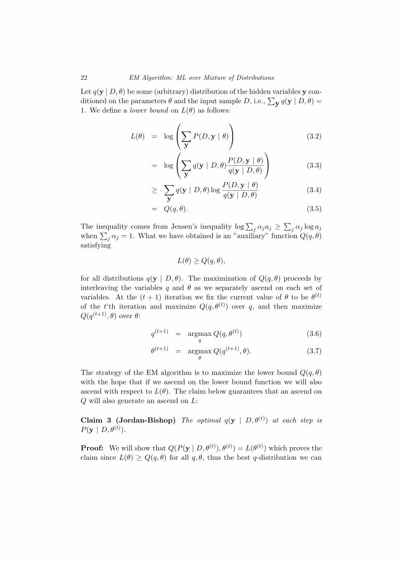
Let q(y |D, θ) be some (arbitrary) distribution of the hidden variables y con-ditioned on the parameters θ and the input sample D, i.e.,
∑y q(y | D, θ) =
1. We define a lower bound on L(θ) as follows:
L(θ) = log
∑yP (D,y | θ)
(3.2)
= log
∑yq(y | D, θ)P (D,y | θ)
q(y | D, θ)
(3.3)
≥∑yq(y | D, θ) log
P (D,y | θ)q(y | D, θ)
(3.4)
= Q(q, θ). (3.5)
The inequality comes from Jensen’s inequality log∑
j αjaj ≥∑
j αj log ajwhen
∑j αj = 1. What we have obtained is an ”auxiliary” function Q(q, θ)
satisfying
L(θ) ≥ Q(q, θ),
for all distributions q(y | D, θ). The maximization of Q(q, θ) proceeds byinterleaving the variables q and θ as we separately ascend on each set ofvariables. At the (t + 1) iteration we fix the current value of θ to be θ(t)
of the t’th iteration and maximize Q(q, θ(t)) over q, and then maximizeQ(q(t+1), θ) over θ:
q(t+1) = argmaxq
Q(q, θ(t)) (3.6)
θ(t+1) = argmaxθ
Q(q(t+1), θ). (3.7)
The strategy of the EM algorithm is to maximize the lower bound Q(q, θ)with the hope that if we ascend on the lower bound function we will alsoascend with respect to L(θ). The claim below guarantees that an ascend onQ will also generate an ascend on L:
Claim 3 (Jordan-Bishop) The optimal q(y | D, θ(t)) at each step isP (y | D, θ(t)).
Proof: We will show that Q(P (y | D, θ(t)), θ(t)) = L(θ(t)) which proves theclaim since L(θ) ≥ Q(q, θ) for all q, θ, thus the best q-distribution we can

3.1 The EM Algorithm: General 23
hope to find is one that makes the lower-bound meet L(θ) at θ = θ(t).
Q(P (y | D, θ(t)), θ(t)) =∑yP (y | D, θ(t)) log
P (D,y | θ(t))P (y | D, θ(t))
=∑yP (y | D, θ(t)) log
P (y | D, θ(t))P (D | θ(t))P (y | D, θ(t))
= logP (D | θ(t))∑yP (y | D, θ(t))
= L(θ(t))
The proof provides also the validity for the approach of ascending alongthe lower bound Q(q, θ) because at the point θ(t) the two functions coincide,i.e., the lower bound function at θ = θ(t) is equal to L(θ(t)) therefore ifwe continue and ascend along Q(·) we are guaranteed to ascend along L(θ)as well† — therefore, convergence is guaranteed. It can also be shown (butomitted here) that the point of convergence is a stationary point of L(θ) (wasshown originally by C.F. Jeff Wu in 1983 years after EM was introduced in1977) under fairly general conditions. The second step of maximizing overθ then becomes:
θ(t+1) = argmaxθ
∑yP (y | D, θ(t)) logP (D,y | θ). (3.8)
This defines the EM algorithm. Often the ”Expectation” step is describedas taking the expectation of:
Ey∼P (y | D,θ(t)) [logP (D,y | θ)] ,
followed by a Maximization step of finding θ that maximizes the expectation— hence the term EM for this algorithm.
Eqn. 3.8 describes a principle but not an algorithm because in general,without making assumptions on the statistical relationship between the datapoints and the hidden variable the problem presented in eqn. 3.8 is unwieldy.We will reduce eqn. 3.8 to something more manageable by making the i.i.d.assumption. This is detailed in the following section.
† this manner of deriving EM was adapted from Jordan and Bishop’s book notes, 2001.

24 EM Algorithm: ML over Mixture of Distributions
3.2 EM with i.i.d. Data
The EM optimization presented in eqn. 3.8 can be simplified if we assumethe data points (and the hidden variable values) are i.i.d.
P (D | θ) =n∏i=1
P (xi | θ), P (D,y | θ) =n∏i=1
P (xi, yi | θ),
and
P (y | D, θ) =n∏i=1
P (yi | xi, θ).
For any α(yi) we have:
∑yα(yi)P (y | D, θ) =
∑y1
· · ·∑yn
α(yi)P (y1 | x1, θ) · · · P (yn | xn, θ)
=∑yi
α(yi)P (yi | xi, θ)
this is because∑
yjP (yj | xj , θ) = 1. Substituting the simplifications above
into eqn. 3.8 we obtain:
θ(t+1) = argmaxθ
k∑j=1
m∑i=1
P (yi = αj | xi, θ(t)) logP (xi, yi = αj | θ) (3.9)
where yi ∈ α1, ..., αk.
3.3 Back to the Coins Example
We will apply the EM scheme to our running example of mixture of Bernoullidistributions. We wish to compute
Q(θ, θ(t)) =∑yP (y | D, θ(t)) logP (D,y | θ)
=n∑i=1
2∑j=1
P (yi = j | xi, θ(t)) logP (xi, yi = j | θ),

3.3 Back to the Coins Example 25
and then maximize Q() with respect to p, q, λ.
Q(θ, θ′) =n∑i=1
[P (yi = 1 | xi, θ′) logP (xi | yi = 1, θ)P (yi = 1 | θ)
]+
n∑i=1
[P (yi = 2 | xi, θ′) logP (xi | yi = 2, θ)P (yi = 2 | θ)
]=
∑i
[µi log(λpni(1− p)(3−ni)) + (1− µi) log((1− λ)qni(1− q)(3−ni))
]where θ′ stands for θ(t) and µi = P (yi = 1 | xi, θ′). The values of µi areknown since θ′ = (λo, po, qo) are given from the previous iteration. TheBayes formula is used to compute µi:
µi = P (yi = 1 | xi, θ′) =P (xi | yi = 1, θ′)P (yi = 1 | θ′)
P (xi | θ′)
=λop
nio (1− po)(3−ni)
λopnio (1− po)(3−ni) + (1− λo)qnio (1− qo)(3−ni)
We wish to compute: maxp,q,λQ(θ, θ′). The partial derivative with respectto λ is:
∂Q
∂λ=∑i
µi1λ−∑i
(1− µi)1
1− λ= 0,
from which we obtain the update formula of λ given µi:
λ =1k
n∑i=1
µi.
The partial derivative with respect to p is:
∂Q
∂p=∑i
µinip−∑i
µi(3− ni)1− p
= 0,
from which we obtain the update formula:
p =1∑i µi
∑i
ni3µi.
Likewise the update rule for q is:
q =1∑
i(1− µi)∑i
ni3
(1− µi).
To conclude, we start with some initial ”guess” of the values of p, q, λ, com-pute the values of µi and update iteratively the values of p, q, λ where at theend of each iteration the new values of µi are computed.
26 EM Algorithm: ML over Mixture of Distributions
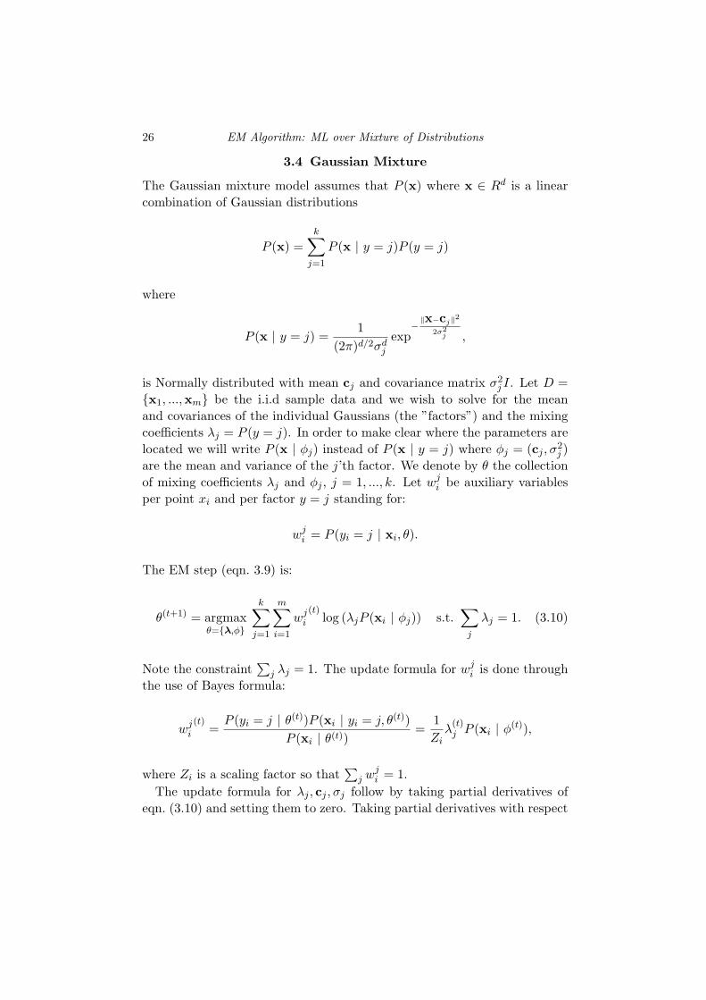
3.4 Gaussian Mixture
The Gaussian mixture model assumes that P (x) where x ∈ Rd is a linearcombination of Gaussian distributions
P (x) =k∑j=1
P (x | y = j)P (y = j)
where
P (x | y = j) =1
(2π)d/2σdjexp−‖x−cj‖2
2σ2j ,
is Normally distributed with mean cj and covariance matrix σ2j I. Let D =
x1, ...,xm be the i.i.d sample data and we wish to solve for the meanand covariances of the individual Gaussians (the ”factors”) and the mixingcoefficients λj = P (y = j). In order to make clear where the parameters arelocated we will write P (x | φj) instead of P (x | y = j) where φj = (cj , σ2
j )are the mean and variance of the j’th factor. We denote by θ the collectionof mixing coefficients λj and φj , j = 1, ..., k. Let wji be auxiliary variablesper point xi and per factor y = j standing for:
wji = P (yi = j | xi, θ).
The EM step (eqn. 3.9) is:
θ(t+1) = argmaxθ=λ,φ
k∑j=1
m∑i=1
wji(t)
log (λjP (xi | φj)) s.t.∑j
λj = 1. (3.10)
Note the constraint∑
j λj = 1. The update formula for wji is done throughthe use of Bayes formula:
wji(t)
=P (yi = j | θ(t))P (xi | yi = j, θ(t))
P (xi | θ(t))=
1Ziλ
(t)j P (xi | φ(t)),
where Zi is a scaling factor so that∑
j wji = 1.
The update formula for λj , cj , σj follow by taking partial derivatives ofeqn. (3.10) and setting them to zero. Taking partial derivatives with respect

3.5 Application Examples 27
to λj , cj and σj we obtain the update rules:
λj =1m
m∑i=1
wji
cj =1∑iw
ji
m∑i=1
wjixi,
σ2j =
1
d∑
iwji
m∑i=1
wji ‖xi − cj‖2.
In other words, the observations xi are weighted by wji before a Gaussian isfitted (k times, one for each factor).
3.5 Application Examples
3.5.1 Gaussian Mixture and Clustering
The Gaussian mixture model is classically used for clustering applications.In a clustering application one receives a sample of points x1, ...,xm whereeach point resides in Rd. The task of the learner (in this case ”unsupervised”learning) is to group the m points into k sets. Let yi ∈ 1, ..., k wherei = 1, ...,m stands for the required labeling. The clustering solution is anassignment of values to y1, ..., ym according to some clustering criteria.
In the Gaussian mixture model points are clustered together if they arisefrom the same Gaussian distribution. The EM algorithm provides a proba-bilistic assignment P (yi = j | xi) which we denoted above as wji .
3.5.2 Multinomial Mixture and ”bag of words” Application
The multinomial mixture (the coins example we toyed with) is typically usedfor representing ”count” data, such as when representing text documents ashigh-dimensional vectors. A vector representation of a text document asso-ciates a word from a fixed vocabulary to a coordinate entry of the vector.The value of the entry represents the number of times that particular wordappeared in the document. If we ignore the order in which the words ap-peared and count only their frequency, a set of documents d1, ..., dm and aset of words w1, ...., wn could be jointly represented by a co-occurence n×mmatrix G where Gij contains the number of times word wi appeared in doc-ument dj . If we scale G such that
∑ij Gij = 1 then we have a distribution
P (w, d). This kind of representation of a set of documents is called ”bag ofwords”.
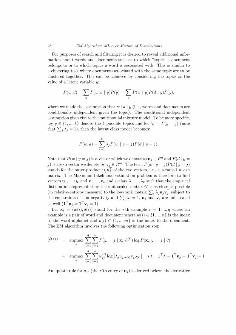
28 EM Algorithm: ML over Mixture of Distributions
For purposes of search and filtering it is desired to reveal additional infor-mation about words and documents such as to which ”topic” a documentbelongs to or to which topics a word is associated with. This is similar toa clustering task where documents associated with the same topic are to beclustered together. This can be achieved by considering the topics as thevalue of a latent variable y:
P (w, d) =∑y
P (w, d | y)P (y) =∑y
P (w | y)P (d | y)P (y),
where we made the assumption that w⊥d | y (i.e., words and documents areconditionally independent given the topic). The conditional independentassumption gives rise to the multinomial mixture model. To be more specific,ley y ∈ 1, ..., k denote the k possible topics and let λj = P (y = j) (notethat
∑j λj = 1), then the latent class model becomes:
P (w, d) =k∑j=1
λjP (w | y = j)P (d | y = j).
Note that P (w | y = j) is a vector which we denote as uj ∈ Rn and P (d | y =j) is also a vector we denote by vj ∈ Rm. The term P (w | y = j)P (d | y = j)stands for the outer-product ujv>j of the two vectors, i.e., is a rank-1 n×mmatrix. The Maximum-Likelihood estimation problem is therefore to findvectors u1, ...,uk and v1, ...,vk and scalars λ1, ..., λk such that the empiricaldistribution represented by the unit scaled matrix G is as close as possible(in relative-entropy measure) to the low-rank matrix
∑j λjujv
>j subject to
the constraints of non-negativity and∑
j λj = 1, uj and vj are unit-scaledas well (1>uj = 1>vj = 1).
Let xi = (w(i), d(i)) stand for the i’th example i = 1, ..., q where anexample is a pair of word and document where w(i) ∈ 1, ..., n is the indexto the word alphabet and d(i) ∈ 1, ...,m is the index to the document.The EM algorithm involves the following optimization step:
θ(t+1) = argmaxθ
q∑i=1
k∑j=1
P (yi = j | xi, θ(t)) logP (xi, yi = j | θ)
= argmaxθ
q∑i=1
k∑j=1
w(t)ij log
[λjuj,w(i)vj,d(i)
]s.t. 1>λ = 1>uj = 1>vj = 1
An update rule for ujr (the r’th entry of uj) is derived below: the derivative

3.5 Application Examples 29
of the Lagrangian is:
∂
∂ujr
[q∑i=1
w(t)ij log uj,w(i) − µujr
]
=∂
∂ujr
N(r) log ujr∑w(i)=r
w(t)ij − µujr
=N(r)
∑w(i)=r w
(t)ij
ujr− µ = 0
where N(r) stands for the frequency of the word wr in all the documentsd1, ..., dm. Note that N(r) is the result of summing-up the r’th row of G andthat the vector N(1), ..., N(n) is the marginal P (w) =
∑d P (w, d). Given
the constraint 1>uj = 1 we obtain the update rule:
ujr ←N(r)
∑w(i)=r w
(t)ij∑n
s=1N(s)∑
w(i)=sw(t)ij
.
Update rules for the remaining unknowns are similarly derived. Once EMhas converged, then
∑w(i)=r w
∗ij is the probability of the word wr to belong
to the j’th topic and∑
d(i)=sw∗ij is the probability that the s’th document
comes from the j’th topic.
4
Support Vector Machines and Kernel Functions
In this lecture we begin the exploration of the 2-class hyperplane separationproblem. We are given a training set of instances xi ∈ Rn, i = 1, ...,m,and class labels yi = ±1 (i.e., the training set is made up of “positive”and “negative” examples). We wish to find a hyperplane direction w ∈ Rnand an offset scalar b such that w · xi − b > 0 for positive examples andw · xi − b < 0 for negative examples — which together means that themargins yi(w · xi − b) > 0 are positive.
Assuming that such a hyperplane exists, clearly it is not unique. Wetherefore need to introduce another constraint so that we could find themost “sensible” solution among all (infinitley many) possible hyperplaneswhich separate the training data. Another issue is that the framework isvery limited in the sense that for most real-world classification problemsit is somewhat unlikely that there would exist a linear separating functionto begin with. We therefore need to find a way to extend the frameworkto include non-linear decision boundaries at a reasonable cost. These twoissues will be the focus of this lecture.
Regarding the first issue, since there is more than one separating hyper-plane (assuming the training data is linearly separable) then the questionwe need to ask ourselves is among all those solutions which of them has thebest “generalization” properties? In other words, our goal in constructinga learning machine is not necessarily to do very well (or perfect) on thetraining data, because the training data is merely a sample of the instancespace, and not necessarily a “representative” sample — it is simply a sample.Therefore, doing well on the sample (the training data) does not necessarilyguarantee (or even imply) that we will do well on the entire instance space.The goal of constructing a learning machine is to maximize the performanceon the test data (the instances we haven’t seen), which in turn means that
30
4.1 Large Margin Classifier as a Quadratic Linear Programming 31
we wish to generalize “good” classification performance on the training setonto the entire instance space.
A related issue to generalization is that the distribution used to generatethe training data is unknown. Unlike the statistical inference material wehad so far, this time we will not attempt to estimate the distribution. Thereason one can derive optimal learning algorithms yet bypass the need forestimating distributions would be explained later in the course when PAC-learning will be introduced. For now we will focus only on the algorithmicaspect of the learning problem.
The idea is to consider a subset Cγ of all hyperplanes which have a fixedmargin γ where the margin is defined as the distance of the closest trainingpoint to the hyperplane:
γ = mini
yi(w>xi − b)‖w‖
.
The Support Vector Machine (SVM), first introduced by Vapnik and hiscolleagues in 1992, seeks a separating hyperplane which simultaneously min-imizes the empirical error and maximizes the margin. The idea of maximiz-ing the margin is intuitively appealing because a decision boundary whichlies close to some of the training instances is less likely to generalize wellbecause the learning machine will be susceptible to small perturbations ofthose instance vectors. A formal motivation for this approach is deferred tothe PAC-learning material we will introduce later in the course.
4.1 Large Margin Classifier as a Quadratic Linear Programming
We would first like to set up the linear separating hyperplane as an optimiza-tion problem which is both consistent with the training data and maximizesthe margin induce by the separating hyperplane over all possible consistenthyperplanes.
Formally speaking, the distance between a point x and the hyperplane isdefined by
| w · x− b |√w ·w
.
Since we are allowed to scale the parameters w, b at will (note that if w ·x − b > 0 so is (λw) · x − (λb) > 0 for all λ > 0) we can set the distancebetween the boundary points to the hyperplane to be 1/
√w ·w by scaling
w, b such the point(s) with smallest margin (closest to the hyperplane) willbe normalized: | w ·x−b |= 1, therefore the margin is simply 2/
√w ·w (see
Fig. 5.1). Note that argmaxw2/√
w ·w is equivalent to argmaxw2/(w ·w)
32 Support Vector Machines and Kernel Functions
which in turn is equivalent to argminw12w · w. Since all positive points
and negative points should be farther away from the boundary points wealso have the separability constraints w · x − b ≥ 1 when x is a positiveinstance and w ·x−b ≤ −1 when x is a negative instance. Both separabilityconstraints can be combined: y(w · x − b) ≥ 1. Taken together, we havedefined the following optimization problem:
minw,b
12w ·w (4.1)
subject to
yi(w · xi − b)− 1 ≥ 0 i = 1, ...,m (4.2)
This type of optimization problem has a quadratic criteria function andlinear inequalities and is known in the literature as a Quadratic Linear Pro-gramming (QP) type of problem.
This particular QP, however, requires that the training data are linearlyseparable — a condition which may be unrealistic. We can relax this condi-tion by introducing the concept of a “soft margin” in which the separabilityholds approximately with some error:
minw,b,εi
12w ·w + ν
l∑i=1
εi (4.3)
subject to
yi(w · xi − b) ≥ 1− εi i = 1, ...,m
εi ≥ 0
Where ν is some pre-defined weighting factor. The (non-negative) vari-ables εi allow data points to be miss-classified thereby creating an approx-imate separation. Specifically, if xi is a positive instance (yi = 1) then the“soft” constraint becomes:
w · xi − b ≥ 1− εi,
where if εi = 0 we are back to the original constraint where xi is either aboundary point or laying further away in the half space assigned to positiveinstances. When εi > 0 the point xi can reside inside the margin or even inthe half space assigned to negative instances. Likewise, if xi is a negativeinstance (yi = −1) then the soft constraint becomes:
w · xi − b ≤ −1 + εi.
4.1 Large Margin Classifier as a Quadratic Linear Programming 33
),( bw
maximize the margin
||2w
0>i!
0>iµ 0=jµ
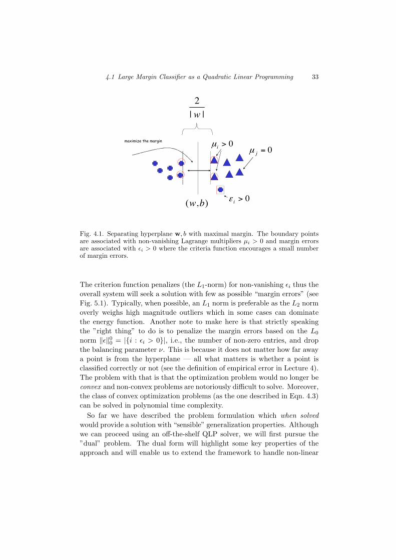
Fig. 4.1. Separating hyperplane w, b with maximal margin. The boundary pointsare associated with non-vanishing Lagrange multipliers µi > 0 and margin errorsare associated with εi > 0 where the criteria function encourages a small numberof margin errors.
The criterion function penalizes (the L1-norm) for non-vanishing εi thus theoverall system will seek a solution with few as possible “margin errors” (seeFig. 5.1). Typically, when possible, an L1 norm is preferable as the L2 normoverly weighs high magnitude outliers which in some cases can dominatethe energy function. Another note to make here is that strictly speakingthe ”right thing” to do is to penalize the margin errors based on the L0
norm ‖ε‖00 = |i : εi > 0|, i.e., the number of non-zero entries, and dropthe balancing parameter ν. This is because it does not matter how far awaya point is from the hyperplane — all what matters is whether a point isclassified correctly or not (see the definition of empirical error in Lecture 4).The problem with that is that the optimization problem would no longer beconvex and non-convex problems are notoriously difficult to solve. Moreover,the class of convex optimization problems (as the one described in Eqn. 4.3)can be solved in polynomial time complexity.
So far we have described the problem formulation which when solvedwould provide a solution with “sensible” generalization properties. Althoughwe can proceed using an off-the-shelf QLP solver, we will first pursue the”dual” problem. The dual form will highlight some key properties of theapproach and will enable us to extend the framework to handle non-linear

34 Support Vector Machines and Kernel Functions
decision surfaces at a very little cost. In the appendix we take a brief tour onthe basic principles associated with constrained optimization, the Karush-Kuhn-Tucker (KKT) theorem and the dual form. Those are recommendedto read before moving to the next section.
4.2 The Support Vector Machine
We return now to the primal problem (eqn. 6.3) representing the maximalmargin separating hyperplane with margin errors:
minw,b,εi
12w ·w + ν
l∑i=1
εi
subject to
yi(w · xi − b) ≥ 1− εi i = 1, ...,m
εi ≥ 0
We will now derive the Lagrangian Dual of this problem. By doing so anew key property will emerge facilitated by the fact that the criteria func-tion θ(µ) (note there are no equality constraints thus there is no need for λ)involves only inner-products of the training instance vectors xi. This prop-erty will form the key of mapping the original input space of dimension n toa higher dimensional space thereby allowing for non-linear decision surfacesfor separating the training data.
Note that with this particular problem the strong duality conditions aresatisfied because the criteria function and the inequality constraints form aconvex set. The Lagrangian takes the following form:
L(w, b, εi, µ) =12w ·w + ν
m∑i=1
εi −m∑i=1
µi [yi(w · xi − b)− 1 + εi]−m∑i=1
δiεi
Recall that
θ(µ) = minw,b,ε
L(w, b, ε,µ, δ).
Since the minimum is obtained at the vanishing partial derivatives of theLagrangian with respect to w, b, the next step would be to evaluate those

4.2 The Support Vector Machine 35
constraints and substitute them back into L() to obtain θ(µ):
∂L
∂w= w−
∑i
µiyixi = 0 (4.4)
∂L
∂b=
∑i
µiyi = 0 (4.5)
∂L
∂εi= ν − µi − δi = 0 (4.6)
From the first constraint (4.4) we obtain w =∑
i µiyixi, that is, w is de-scribed by a linear combination of a subset of the training instances. Thereason that not all instances participate in the linear superposition is dueto the KKT conditions: µi = 0 when yi(w · xi − b) > 1, i.e., the instance xiis classified correctly and is not a boundary point, and conversely, µi > 0when yi(w · xi − b) = 1 − εi, i.e., when xi is a boundary point or whenxi is a margin error (εi > 0) — note that for a margin error instance thevalue of εi would be the smallest possible required to reach an equality inthe constraint because the criteria function penalizes large values of εi. Theboundary points (and the margin errors) are called support vectors thus w isdefined by the support vectors only. The third constraint (4.6) is equivalentto the constraint:
0 ≤ µi ≤ ν i = 1, ..., l,
since δi ≥ 0. Also note that if εi > 0, i.e., point xi is a margin-error point,then by KKT conditions we must have δi = 0. As a result µi = ν. Thereforebased on the values of µi alone we can make the following classifications:
• 0 < µi < ν: point xi is on the margin and is not a margin-error.• µi = ν: points xi is a margin-error point.• µi = 0: point xi is not on the margin.
Substituting these results/constraints back into the Lagrangian L() weobtain the dual problem:
maxµ1,...,µm
θ(µ) =m∑i=1
µi −12
∑i,j
µiµjyiyjxi · xj (4.7)
subject to
0 ≤ µi ≤ ν i = 1, ...,mm∑i=1
yiµi = 0
The criterion function θ(µ) can be written in a more compact manner as

36 Support Vector Machines and Kernel Functions
follows: Let M be a l × l matrix whose entries are Mij = yiyjxi · xj thenθ(µ) = µ>1− 1
2µ>Mµ where 1 is the vector of (1, ..., 1) and µ is the vector(µ1, ..., µm) and µ> is the transpose (row vector). Note that M is positivedefinite, i.e., x>Mx > 0 for all vectors x 6= 0 — a property which will beimportant later.
The key feature of the dual problem is not so much that it is simplerthan the primal (in fact it isn’t since the primal has no equality constraints)or that it has a more “elegant” feel, the key feature is that the problemis completely described by the inner products of the training instances xi,i = 1, ...,m. This fact will be shown to be a crucial ingredient in the so called“kernel trick” for the computation of inner-products in high dimensionalspaces using simple functions defined on pairs of training instances.
4.3 The Kernel Trick
We ended with the dual formulation of the SVM problem and noticed thatthe input data vectors xi are represented by the Gram matrix M . In otherwords, only inner-products of the input vectors play a role in the dual for-mulation — there is no explicit use of xi or any other function of xi besidesinner-products. This observation suggests the use of what is known as the”kernel trick” to replace the inner-products by non-linear functions.
The common principle of kernel methods is to construct nonlinear vari-ants of linear algorithms by substituting inner-products by nonlinear kernelfunctions. Under certain conditions this process can be interpreted as map-ping of the original measurement vectors (so called ”input space”) ontosome higher dimensional space (possibly infinitely high) commonly referredto as the ”feature space”. Mathematically, the kernel approach is definedas follows: let x1, ...,xl be vectors in the input space, say Rn, and con-sider a mapping φ(x) : Rn → F where F is an inner-product space. Thekernel-trick is to calculate the inner-product in F using a kernel functionk : Rn×Rn → R, k(xi,xj) = φ(xi)>φ(xj), while avoiding explicit mappings(evaluation of) φ().
Common choices of kernel selection include the d’th order polynomialkernels k(xi,xj) = (x>i xj + θ)d and the Gaussian RBF kernels k(xi,xj) =exp(− 1
2σ2 ‖xi − xj‖2). If an algorithm can be restated such that the inputvectors appear in terms of inner-products only, one can substitute the inner-products by such a kernel function. The resulting kernel algorithm can beinterpreted as running the original algorithm on the space F of mappedobjects φ(x).
We know that M of the dual form is positive semi-definite because M
4.3 The Kernel Trick 37
can be written is M = Q>Q where Q = [y1x1, ..., ylxl]. Therefore x>Mx =‖Qx‖2 ≥ 0 for all choices of x (which means that the eigenvalues of M arenon-negative). If the entries of M are to be replaced with yiyjk(xi,xj) thenthe condition we must enforce on the function k() is that it is a positivedefinite kernel function. A positive definite function is defined such thatfor any set of vectors x1, ...,xq and for any values of q the matrix K whoseentries are Kij = k(xi,xj) is positive semi-definite. Formally, the conditionsfor admissible kernels k() are known as Mercer’s conditions summarizedbelow:
Theorem 4 (Mercer’s Conditions) Let k(x, y) be symmetric and contin-uous. The following conditions are equivalent:
(i) k(x, y) =∑∞
i=1 αiφi(x)φi(y) = φ(x)>φ(y) for any uniformly converg-ing series αi > 0.
(ii) for all ψ() satisfying∫x ψ
2(x)dx <∞, then∫x
∫yk(x, y)ψ(x)ψ(y)dxdy ≥ 0
(iii) for all xiqi=1 and for all q, the matrix Kij = k(xi, xj) is positivesemi-definite.
Perhaps the non-obvious condition is No. 1 which allows for the featuremap φ() to have infinitely many coordinates (a vector in Hilbert space). Forexample, as we shall see below, the kernel exp(− 1
2σ2 ‖xi − xj‖2) is an inner-product of two vectors with infinitely many coordinates. We will considernext a number of popular kernels.
4.3.1 The Homogeneous Polynomial Kernel
Let x,y ∈ Rk and define k(x,y) = (x>y)d where d > 0 is a natural number.Then, the corresponding feature map φ(x) has
(k+d−1d
)= O(kd) coordinates
which take the value:
φ(x) =
(√(d
n1, ..., nk
)xn1
1 · · · xnkk
)ni≥0,
Pi ni=d
where(
dn1,...,nk
)= d!/(n1! · · · nk!) is the multinomial coefficient (number of
ways to distribute d balls into k bins where the j’th bin hold exactly nj ≥ 0balls):
(x1 + ...+ xk)d =∑
ni≥0,Pi ni=d
(d
n1, ..., nk
)xn1
1 · · · xnkk .
38 Support Vector Machines and Kernel Functions
The dimension of the vector space φ(x) where x ∈ Rk can be measuredusing the following combinatorial problem: how many arrangements of k−1partitions to be placed among d items? the answer is
(k+d−1k−1
)=(k+d−1d
)=
O(kd). For example, k = d = 2 gives us :
(x>y)2 = x21y
21 + 2x1x2y1y2 + x2
2y22 = φ(x)>φ(y),
where φ(x) = (x21, x
22,√
2x1x2).
4.3.2 The non-homogeneous Polynomial Kernel
The feature map φ(x) contains all monomials whose power is lesser or equalto d, i.e.,
∑i ni ≤ d. This can be acheived by increasing the dimension
to k + 1 where nk+1 is used to fill the gap between∑k
i=1 ni < d and d.Therefore the dimension of φ(x) where x ∈ Rk would be
(k+dd
). We have:
(x>y + θ)d = (x1y1 + ...+ xkyk +√θ√θ)d
=∑
ni≥0,Pk+1i=1 ni=d
(d
n1, ..., nk+1
)xn1
1 yn11 · · · x
nk1 ynk1 · θ
nk+1/2θnk+1/2
Therefore, the entries of the vector φ(x) take the values:
φ(x) =
(√(d
n1, ..., nk+1
)xn1
1 · · · xnkk · θ
nk+1/2
)ni≥0,
Pk+1i=1 ni=d
For example, k = d = 2 gives us :
(x>y + θ)2 = x21y
21 + 2x1x2y1y2 + x2
2y22 + 2θx1y1 + 2θx2y2 + θ = φ(x)>φ(y),
where φ(x) = (x21, x
22,√
2x1x2,√
2θx1,√
2θx2,√θ). In this example, φ() is a
mapping fromR2 toR6 and hyperplanes φ(w)>φ(x)−b = 0 inR6 correspondto conics in R2:
(w21)x2
1 + (w22)x2 + (2w1w2)x1x2 + (2θw1)x1 + (2θw2)x2 + (θ − b) = 0
Assume we would like to find a separating conic (Parabola, Hyperbola,Ellipse) function rather than a line in R2. The discussion so far suggests weconstruct the Gram matrix M in the dual form with the d = 2 polynomialkernel k(x,y) = (x>y+θ)2 for some parameter θ of our choosing. The extraeffort we will need to invest is negligible — simply replace every occurrencex>i xj with (x>i xj + θ)2.

4.3 The Kernel Trick 39
4.3.3 The RBF Kernel
The function k(x,y) = e−‖x−y‖2/2σ2known as a Radial Basis Function
(RBF) is a kernel function but with an infinite expansion. Without loss ofgenerality let σ = 1, then we have:
e−‖x−y‖2/2 = e−‖x‖2/2e−‖y‖
2/2ex>y
=∞∑j=0
(x>y)j
j!e−‖x‖
2/2e−‖y‖2/2
=∞∑j=0
e− ‖x‖22j
√j!1/j
e− ‖y‖
2
2j
√j!1/j
x>y
j
=∞∑j=0
∑Pi ni=j
e− ‖x‖
2
2j
√j!1/j
(j
n1, ..., nk
)1/2
xn11 · · · x
nkk
e− ‖y‖
2
2j
√j!1/j
(j
n1, ..., nk
)1/2
yn11 · · · y
nkk
From which we can see that the entries of the feature map φ(x) are:
φ(x) =
e− ‖x‖22j
√j!1/j
(j
n1, ..., nk
)1/2
xn11 · · · x
nkk
j=0,..,∞,
Pki=1 ni=j
4.3.4 Classifying New Instances
By adopting some kernel k() we are in fact mapping x → φ(x), thus wethen proceed to solve for φ(w) and b using some QLP solver. The QLPsolution of the dual form will yield the solution for the Lagrange multipliersµ1, ..., µm. We saw from eqn. (4.4) that we can express φ(w) as a functionof the (mapped) examples:
φ(w) =∑i
µiyiφ(xi).
Rather than explicitly representing φ(w) — a task which may be prohibitlyexpensive since in general the dimension of the feature space of a polynomialmapping is
(k+dd
)— we store all the support vectors (those input vectors
with corresponding µi > 0) and use them for the evaluation of test examples:
f(x) = sign(φ(w)>φ(x)− b) = sign(∑i
µiyiφ(xi)>φ(x)− b)
= sign(∑i
µiyik(xi,x)− b).

40 Support Vector Machines and Kernel Functions
We see that the kernel trick enabled us to look for a non-linear separatingsurface by making an implicit mapping of the input space onto a higher di-mensional feature space using the same dual form of the SVM formulation —the only change required was in the way the Gram matrix was constructed.The price paid for this convenience is to carry all the support vectors at thetime of classification f(x).
A couple of notes may be worthwhile at this point. The constant b canbe recovered from any of the support vectors. Say, x+ is a positive supportvector (but not a margin error, i.e., µi < ν). Then φ(w)>φ(x+) − b = 1from which b can be recovered. The second note is that the number ofsupport vectors is typically around 10% of the number of training examples(empirically). Thus the computational load during evaluation of f(x) maybe relatively high. Approximations have been proposed in the literature bylooking for a reduced number of support vectors (not necessarily alignedwith the training set) — but this is beyond the scope of this course.
The kernel trick gained its popularity with the introduction of the SVMbut since then has taken a life of its own and has been applied to principalcomponent analysis (PCA), ridge regression, canonical correlation analysis(CCA), QR factorization and the list goes on. We will meet again with thekernel trick later on.

5
Spectral Analysis I: PCA, LDA, CCA
In this lecture (and the following one) we will focus on spectral methods forlearning. Today we will focus on dimensionality reduction using PrincipleComponent Analysis (PCA), multi-class learning using Linear DiscriminantAnalysis (LDA) and Canonical Correlation Analysis (CCA). In the nextlecture we will focus on spectral clustering methods.
Dimensionality reduction appears when the dimension of the input vectoris very large (imagine pixels in an image, for example) while the coordi-nate measurements are highly inter-dependent (again, imagine the redun-dancy present among neighboring pixels in an image). High dimensionaldata impose computational efficiency challenges and often translate to poorgeneralization abilities of the learning engine (see lectures on PAC). A di-mensionality reduction can also be viewed as a feature extraction processwhere one takes as input a large feature set (the original measurements)and creates from them a much smaller number of new features which arethen fed into the learning engine.
In this lecture we will focus on feature extraction from a very specific (andconstrained) stanpoint. We would be looking for a mixing (linear combina-tion) of the input coordinates such that we obtain a linear projection fromRn to Rq for some q < n. In doing so we wish to reduce the redundancywhile preserving as much as possible the variance of the data. From a sta-tistical standpoint this is achieved by transforming to a new set of variables,called principal components, which are uncorrelated so that the first fewretain most of the variation present in all of the original coordinates. Forexample, in an image processing application the input images are highly re-dundant where neighboring pixel values are highly correlated. The purposeof feature extraction would be to transform the input image into a vector ofoutput components with the least redundancy possible. Form a geometricstandpoint, this is achieved by finding the ”closest” (in least squares sense)
41
42 Spectral Analysis I: PCA, LDA, CCA
linear q-dimensional susbspace to the m sample points S. The new sub-space is a lower dimensional ”best approximation” to the sample S. Thesetwo, equivalent, perspectives on data compression (dimensionality reduc-tion) form the central idea of principal component analysis (PCA) whichprobably the oldest (going back to Pearson 1901) and best known of thetechniques of multivariate analysis in statistics. The computation of PCAis very simple and the definition is straightforward, but has a wide varietyof different applications, a number of different derivations, quite a numberof different terminologies (especially outside the statistical literature) and isthe basis for quite a number of variations on the basic technique.
We then extend the variance preserving approach for data representationfor labeled data sets. We will describe the linear classifier approach (sepa-rating hyperplane) form the point of view of looking for a hyperplane suchthat when the data is projected onto it the separation is maximized (the dis-tance between the class means is maximal) and the data within each class iscompact (the variance/spread is minimized). The solution is also produced,just like PCA, by a spectral analysis of the data. This approach goes underthe name of Fisher’s Linear Discriminant Analysis (LDA).
What is common between PCA and LDA is (i) the use of spectral ma-trix analysis — i.e., what can you do with eigenvalues and eigenvectors ofmatrices representing subspaces of the data? (ii) these techniques produceoptimal results for normally distributed data and are very easy to imple-ment. There is a large variety of uses of spectral analysis in statistical andlearning literature including spectral clustering, Multi Dimensional Scaling(MDS) and data modeling in general. Another point to note is that this isthe first time in the course where the type of data distribution plays a rolein the analysis — the two techniques are defined for any distribution butare optimal only under the Gaussian distribution.
We will also describe a non-linear extension of PCA known as Kernel-PCA, but the focus would be mostly on PCA itself and its analysis froma couple of vantage points: (i) PCA as an optimal reconstruction after adimension reduction, i.e., data compression, and (ii) PCA for redundancyreduction (decorrelation) of the output components.
5.1 PCA: Statistical Perspective
Let x1, ...,xm ∈ Rn be our sample data S of vectors in Rn, arranged ascolumns of a matrix A. It will be convenient to assume that the data iscentered, i.e.,
∑xi = 0. If the data is not centered we can always center it
by computing the mean vector µ = (1/m)∑
i xi and replace the original data
5.1 PCA: Statistical Perspective 43
sample with the new sample xi − µ. In a statistical sense, the coordinatesof the vector x ∈ Rn are considered as random variables, thus a row in thematrix A is the sample of values of a particular random variable, drawn fromsome unknown probability distribution, associated with the row position.We wish to find vectors u1, ...,uq (arranged as columns of a matrix U),where q ≤ min(n,m), such that the new feature measurements y = U>x(who are the result of linear combinations u>1 x, ...,u>q x of the original featuremeasurements x) have certain desirable properties.
The idea property to seek from the new coordinates y is statistical inde-pendence, i.e., P (y1, .., yq) = P (y1) · · ·P (yq) which would mean that we haveremoved the redundancy of the original data x in the best possible manner.This goal, however, is too much to ask from a linear transformation andinstead we would ask for a weaker property to hold: that the pairwise co-variance cov(yi, yj) = 0 vanishes, i.e., that the covariance matrix on the newcoordinates is diagonal. A diagonal covariance insures some redundancy re-moval, but not as good as statistical independence. However, when the datais Normally distributed P (x) ∼ N(µ,Σ) with mean µ and covariance Σ, thenthe transformation which diagonalizes the covariance matrix also guaranteesstatistical independence. Among all transformations that de-correlate thedata we will seek the one that maximizes the spread (variance) of the sampledata after being projected onto the new axes vectors.
5.1.1 Maximizing the Variance of Output Coordinates
The property we would like to maximize is that the projection of the sampledata on the new axes is as spread as possible. To start this analysis, assumeq = 1, i.e., the n components of the input vector x are reduced to a singleoutput component y = u>x. We are looking for a single vector u ∈ Rn
whose direction maximizes the variance of the output component y.Formally, we are looking for a unit vector u which maximizes
∑i(u>xi)2
(see Appendix A for basic statistical definitions and note that E[y] = 0because
∑i u>xi = u>i (
∑i xi) = 0). In other words, the projected points
onto the axis represented by the vector u are as spread as possible (in aleast squares sense). In vector notation, the optimization problem takes thefollowing form:
maxu
12‖u>A‖2 subject to
12u>u = 1
The Lagrangian of the problem is:
L(u, λ) =12u>AA>u− λ(
12u>u− 1)
44 Spectral Analysis I: PCA, LDA, CCA
By taking the partial derivative ∂L/∂u = 0 we obtain the following necessarycondition (see Appendix B):
AA>u = λu,
which tells us that u is an eigenvector of the n× n (symmetric and positivedefinite) matrix AA>. There are n eigenvectors associated with AA> andwe can easily convince ourselves that we are looking for the one associatedwith the maximal eigenvalue: substitute λu instead of AA>u in the criterionfunction u>AA>u to obtain λ(u>u) = λ and since the eigenvalues must bepositive (since AA> is positive definite), then the optimum is obtained forthe maximal eigenvalue. The leading eigenvector u of AA> is called the firstprincipal axis of the data sample represented by the columns of the matrixA, and y = u>x is called the first principal component of the data sample.
For convenience, we denote u1 = u and λ1 = λ as the leading eigenvectorand eigenvalue of AA>. Next, we look for y2 = u>2 x which is uncorrelatedwith y1 = u>1 x and which has maximum variance (and so on for u3, ...,uq).Two random variables are uncorrelated if their covariance vanishes. Bydefinition of covariance (see Appendix A) we obtain:
Cov(y1y2) =∑i
(u>1 xi)(u>2 xi) = u>1 (∑i
xix>i )u2
= u>1 AA>u2 = u>2 AA
>u1 = λ1u>1 u2 = 0
We can therefore use the condition u>1 u2 = 0 to specify zero correlationbetween y1, y2. The functional to be optimized becomes:
maxu2
12‖u>2 A‖2 subject to
12u>2 u2 = 1, u>1 u2 = 0,
with the Lagrangian being:
L(u2, λ, δ) =12u>2 AA
>u2 − λ(12u>2 u2 − 1)− δu>1 u2.
By taking the partial derivative with respect to u2 we obtain the necessarycondition:
AA>u2 − λu2 − δu1 = 0.
Multiply the equation by u1 from the left:
u>1 AA>u2 − λu>1 u2 − δu>1 u1 = 0,
and noting from above that u>1 AA>u2 = u>1 u2 = 0 we obtain δ = 0. As a
result we obtain:
AA>u2 = λu2,

5.1 PCA: Statistical Perspective 45
so once more we have that λ,u2 form an eigenvalue/eigenvector pair of AA>.As before, λ should be as large as possible from the remaining spectral de-composition. By induction, it can be shown that the remaining principalvectors u3, ...,uq are the decreasing order eigenvactors of AA> and the vari-ance of the i’th principal component yi = u>i x is λi.
Taken together, the PCA is the solution of the following optimizationproblem:
maxu1,...,uq
12
∑i
‖u>i A‖2 subject to u>i ui = 1, u>i uj = 0, i 6= j = 1, ..., q.
It will be useful for later to write the optimization function in a more concisemanner as follows. Let U be the n × q matrix whose columns are ui andD = diag(λ1, ..., λq) is an q×q diagonal matrix and λ1 ≥ λ2 ≥ ... ≥ λq. Thenfrom above we have that U>U = I and AA>U = UD. Using the fact thattrace(xy>) = x>y, trace(AB) = trace(BA) and trace(A+B) = trace(A)+trace(B) we can convert
∑i ‖u>i A‖2 to trace(U>AA>U) as follows:
∑i
u>i AA>ui =
∑i
trace(A>uiu>i A) = trace(A>(∑i
uiu>i )A)
= trace(A>UU>A) = trace(U>AA>U)
Thus, PCA becomes the solution of the following optimization function:
maxU∈Rn×q
trace(U>AA>U) subject to U>U = I. (5.1)
The solution, as saw above, is that U = [u1, ...,uq] consists of the decreasingorder eigenvectors of AA>. At the optimum, trace(U>AA>U) is equal totrace(D) which is equal to the sum of eigenvalues λ1 + ...+ λq.
It is worthwhile noting that when q = n, UU> = U>U = I, and the PCAtransform is a change of basis in Rn known as Karhunen-Loeve transform.
To conclude, the PCA transform looks for q orthogonal direction vectors(called the principal axes) such that the projection of input sample vectorsonto the principal directions has the maximal spread, or equivalently thatthe variance of the output coordinates y = U>x is maximal. The principaldirections are the leading (with respect to descending eigenvalues) q eigen-vectors of the matrix AA>. When q = n, the principal directions form abasis of Rn with the property of de-correlating the data and maximizing thevariance of the coordinates of the sample input vectors.
46 Spectral Analysis I: PCA, LDA, CCA
5.1.2 Decorrelation: Diagonalization of the Covariance Matrix
In the previous section we saw that PCA generates a new coordinate systemy = U>x where the coordinates y1, ..., yq of x in the new system are uncorre-lated. This means that the covariance matrix over the principle componentsshould be diagonal. In this section we will explore this perspective in moredetail.
The covariance matrix Σx of the sample data x1, ...,xm with zero meanis
(1/m)∑i
xix>i = (1/m)AA>,
therefore the matrix AA> we derived above is a scaled version of the co-variance of the sample data (see Appendix A). The scale factor 1/m wasunimportant in the process above because the eigenvectors are of unit norm,thus any scale of AA> would produce the same set of eigenvectors.
The off-diagonal entries of the covariance matrix Σx represent the corre-lation (a measure of statistical dependence) between the i’th and j’th com-ponent vectors, i.e., the entries of the input vectors x. The existence ofcorrelations among the components (features) of the input signal is a signof redundancy, therefore from the point of view of transforming the inputrepresentation into one which is less redundant, we would like to find atransformation y = U>x with an output representation y which is associ-ated with a diagonal covariance matrix Σy, i.e., the components of y areuncorrelated.
Formally, Σy = (1/m)∑
i yiy>i = (1/m)U>AA>U , therefore we wish to
find an n × q matrix for which U>AA>U is diagonal. If in addition, wewould require that the variance of the output coordinates is maximized,i.e., trace(U>AA>U) is maximal (but then we need to constrain the lengthof the column vectors of U , i.e., set ‖ui‖ = 1) then we would get a uniquesolution for U where the columns are orthonormal and are defined as the firstq eigenvectors of the covariance matrix Σx. This is exactly the optimizationproblem defined by eqn. (5.1).
We see therefore that PCA “decorrelates” the input data. Decorrelationand statistical independence are not the same thing. If the coordinates arestatistically independent then the covariance matrix is diagonal†, but it doesnot follow that uncorrelated variables must be statistically independent —covariance is just one measure of dependence. In fact, the covariance is ameasure of pairwise dependency only. However, it is a fact that uncorrelated
† σxy =Px
Py(x − µx)(y − µy)p(x, y) =
Px
Py(x − µx)(y − µy)p(x)(p(y) = (
Px(x −
µx)p(x))(Py(y − µy)p(y)) = 0

5.2 PCA: Optimal Reconstruction 47
variables are statistically independent if they have a multivariate normaldistribution (a Gaussian). In other words, if the sample data x are drawnfrom a probability distribution p(x) which has Gaussian form, the PCAtransforms the sample data into a statistically independent set of variablesy = U>x. The details are explained below.
Recall that a multivariate normal distribution of the random variablesx = (x1, ..., xn)> is defined as p(x) ≈ N(µ,Σ):
p(x) =1
(2π)n/2|Σ|1/2e−
12
(x−µ)>Σ−1(x−µ).
Also recall that a linear combination of the variables produces also a normaldistribution N(U>µ,U>ΣU):
Σy =∑y
(y−µy)(y−µy)> =∑x
(U>x−U>µx)(U>x−U>µx)> = U>ΣxU,
therefore choose U such that Σy = U>ΣU is a diagonal matrix Σy =diag(σ2
1, ..., σ2n). We have in that case:
p(x) =1
(2π)n/2∏i σi
e− 1
2
Pi
“xi−µiσi
”2
which can be written as a product of univariate normal distributions pxi(xi):
p(x) =n∏i=1
1(2π)1/2σi
e− 1
2
“xi−µiσi
”2
=n∏i=1
pxi(xi),
which proves the assertion that decorrelated normally distributed variablesare statistically independent.
5.2 PCA: Optimal Reconstruction
A different, yet equivalent, perspective on the PCA transformation is as anoptimal reconstruction (in a least squares sense) after a dimension reduction.We are given a sample data as before x1, ...,xm and we are looking for a smallnumber of orthonormal principal vectors u1, ...,uq where q < min(n, k)which define a q-dimensional linear subspace of Rn which best approximatethe original input vectors in a least squares sense. In other words, theprojection xi of the sample points xi onto the q-dimensional subspace shouldminimize
∑i ‖xi − xi‖2 over all possible q-dimensional subspaces of Rn.
Let U be the subspace spanned by the principal vectors (columns of U)and let P be the n× n projection matrix mapping a point x ∈ Rn onto itsprojection x ∈ U . From the definition of projection, the vector x− x must
48 Spectral Analysis I: PCA, LDA, CCA
be orthogonal to the subspace U . Let y = (y1, ..., yq) be the coordinates of xwith respect to the principal vectors, i.e., Uy = x. Then, from orthogonalitywe have that (x − Uy)>Uw = 0 for all vectors w ∈ Rn. Since this is truefor all w then U>Uy − U>x = 0. Therefore, y = (U>U)−1U>x and as aresult the projection matrix P becomes:
P = U(U>U)−1U>,
satisfying Px = x. In the case the columns of U are orthonormal, U>U = I,we have P = UU>. We are ready now to describe the optimization problemon U : we wish to find an orthonormal set of principal vectors, U>U = I,such that
∑i ‖xi − UU>xi‖2 is minimized.
Note that∑
i ‖xi − UU>xi‖2 = ‖A − UU>A‖2F where ‖B‖2F =∑
i,j b2ij
is the square Frobenious norm of a matrix. The optimal reconstructionproblem therefore becomes:
minU‖A− UU>A‖2F subject to U>U = I.
We will show now that:
argminU
‖A− UU>A‖2F = argmaxU
trace(U>AA>U),
which shows that the optimal reconstruction problem is solved by PCA(recall Eqn. 5.1).
From the identity ‖B‖2F = trace(BB>), we have:
‖A− UU>A‖2F = trace((A− UU>A)(A− UU>A)>).
Expanding the right hand side gives us:
trace((A− UU>A)(A− UU>A)>) = trace(AA>)− trace(AA>UU>)
− trace(UU>AA>) + trace(UU>AA>UU>)
The second and third term are equal (commutativity of trace) and is alsoequal to the 4th term due to commutativity of the trace and U>U = I.Taken together:
‖A− UU>A‖2F = trace(AA>)− trace(U>AA>U).
To conclude, we have proven that by taking the first q eigenvectors of AA>
we obtain a linear subspace which is as close as possible (in a least squaressense) to the original sample data. Hence, PCA can be viewed as a vehi-cle for optimal reconstruction after dimension reduction. The optimization

5.3 The Case n >> m 49
problem whose solution is the leading q eigenvectors of AA> is described ineqn. 5.1:
maxU∈Rn×q
trace(U>AA>U) subject to U>U = I.
5.3 The Case n >> m
Consider the situation where n, the dimension of the input vectors, is rela-tively large compared to the number of sample vectors m. For example, con-sider input vectors representing 50× 50 sized images of faces, i.e., n = 2500,where m = 100. In other words, we are looking for a small number of “facetemplates” (known as “eigenfaces”) which approximate well the original setof 100 face images. In this case, AA> is very large, 2500×2500, yet the num-ber of non-vanishing eigenvalues cannot be higher than 100. Given that theeigendecomposition process is O(25003), the computational burden wouldbe very high. However, it is possible to perform an eigendecomposition onA>A (a 100× 100 matrix) instead, as shown next.
Let the columns ofQ be the first q < m eigenvectors of A>A, i.e., A>AQ =QD where D is diagonal containing the corresponding eigenvalues. Afterpre-multiplying both sides by A we obtain:
AA>(AQ) = (AQ)D,
from which we conclude that AQ contains the first q eigenvectors (but un-normalized) of AA>. We have therefore that U = AQD−
12 because:
U>U = D−12Q>A>AQD−
12 = D−
12DD−
12 = I,
where we used the fact that Q>A>AQ = D. Note that eigenvalues of A>Aand AA> are the same (because AA>(AQD−
12 ) = (AQD−
12 )D).
5.4 Kernel PCA
We can take the case n >> m described in the previous section one step fur-ther and consider such large values of n which are practically uncomputable— a situation which results when mapping the original input vectors to ahigh dimensional space: φ(x) where φ : Rn → F for which dim(F) >> n.For example, φ(x) representing the d’th order monomials of the coordinatesof x, i.e., dim(F) =
(n+d−1
d
)which is exponential in d. The mappings
of interest are those which are paired with a non-linear kernel function:k(x,x′) = φ(x)>φ(x′).
Performing PCA on A = [φ(x1), ..., φ(xm)] is equivalent to finding the

50 Spectral Analysis I: PCA, LDA, CCA
non-linear surface in Rn (the nature of the non-linearity depends on thechoice of φ()) which best approximates the original sample data x1, ...,xm.The problem is that AA> is not computable — however A>A is computablebecause (A>A)ij = k(xi,xj).
From the previous section, U = AQD−12 = AV contains the first q eigen-
vectors of AA>(where Q and D are computable). Since A itself is notcomputable we cannot represent U explicitly, but we can project a newvector φ(x) onto the principal directions u1, ...,uq and obtain the principalcomponents, i.e., the output vector y = U>φ(x), as follows.
y = U>φ(x) = V >A>φ(x) = V >
k(x1,x)
.
.
.
k(xm,x)
.
Given the principal components (entries of y = U>φ(x) of φ(x)) we canmeasure, for example, the distance between φ(x) and the projection ˆφ(x) =UU>φ(x) = Uy onto the linear subspace spanned by u1, ...,uq (without theneed to explicitly compute the principal axes ui), as follows.
‖φ(x)− ˆφ(x)‖2 = φ(x)>φ(x) + ˆφ(x)> ˆφ(x)− 2φ(x)> ˆφ(x)
= k(x,x) + y>U>Uy− 2φ(x)>(UU>φ(x))
= k(x,x)− y>y− 2y>y
= k(x,x)− ‖y‖2
5.5 Fisher’s LDA: Basic Idea
We now extend the variance preserving approach for data representation forlabeled data sets. We will focus on 2-class sets and look for a separatinghyperplane:
f(x) = w>x + b,
such that x belongs to the first class if f(x) > 0 and x belongs to the secondclass if f(x) < 0. In the statistical literature this type of function is calleda linear discriminant function. The decision boundary is given by the setof points satisfying f(x) = 0 which is a hyperplane. Fisher’s (1936) LinearDiscriminant Analysis (LDA) is a variance preserving approach for findinga linear discriminant function.

5.5 Fisher’s LDA: Basic Idea 51
Fig. 5.1. Linear discriminant analysis based on class centers alone is not sufficient.Seeking a projection which maximizes the distance between the projected centerswill prefer the horizontal axis over the vertical, yet the two classes overlap on thehorizontal axis. The projected distance along the vertical axis is smaller yet theclasses are better separated. The conclusion is that the sample variance of the twoclasses must be taken into consideration as well.
We will then introduce another popular statistical technique called Canon-ical Correlation Analysis (CCA) for learning the mapping between input andoutput vectors using the notion ”angle” between subspaces.
What is common in the three techniques PCA, LDA and CCA is the useof spectral matrix analysis — i.e., what can you do with eigenvalues andeigenvectors of matrices representing subspaces of the data? These tech-niques produce optimal results for normally distributed data and are veryeasy to implement. There is a large variety of uses of spectral analysis instatistical and learning literature including spectral clustering, Multi Di-mensional Scaling (MDS) and data modeling in general.
To appreciate the general idea behind Fisher’s LDA consider Fig. 5.1. Letthe centers of classes one and two be denoted by µ1 and µ2 respectively. Alinear discriminant function is a projection onto a 1D subspace such thatthe classes would be separated the most in the 1D subspace. The obviousfirst step in this kind of analysis is to make sure that the projected centersµ1, µ2 would be separated as much as possible. We can easily see that thedirection of the 1D subspace should be proportional to µ1 − µ2 as follows:
(µ1 − µ2)2 =(
w>µ1
‖w‖− w>µ2
‖w‖
)2
=(
w>
‖w‖(µ1 − µ2)
)2
.
The right-hand term is maximized when w ≈ µ1 − µ2. As illustrated in
52 Spectral Analysis I: PCA, LDA, CCA
Fig. 5.1, this type of consideration is not sufficient to capture separabilityin the projected subspace because the spread (variance) of the data pointsaround their centers also play an important role. For example, the horizontalaxis in the figure separates the centers better than the vertical axis but onthe other hand does a worse job in separating the classes themselves becauseof the way the data points are spread around their centers. The argumentin favor of separating the centers would work if the data points were livingin a hyper-sphere around the centers, but will not be sufficient otherwise.
The basic idea behind Fisher’s LDA is to consider the sample covariancematrix of the individual classes as well as their centers, in the following way.The optimal 1D projection would that which maximizes the variance of theprojected centers while minimizes the variance of the projected data pointsof each class separately. Mathematically, this idea can be implemented bymaximizes the following ratio:
maxw
(µ1 − µ2)2
s21 + s2
2
,
where s21 is the scaled variance of the projected points of the first class:
s21 =
∑xi∈C1
(xi − µ1)2,
and likewise,
s22 =
∑xi∈C2
(xi − µ2)2,
where x = w>‖w‖xi + b.
We will now formalize this approach and derive its solution. We will beginwith a general description of a multiclass problem where the sample datapoints belong to q different classes, and later focus on the case of q = 2.
5.6 Fisher’s LDA: General Derivation
Let the sample data points S be members of q classes C1, ..., Cq where thenumber of points belonging to class Ci is denoted by li and the total numberof the training set is l =
∑i li. Let µj denote the center of class Ci and µ
denote the center of the complete training set S:
µj =1lj
∑bfxi∈Cj
xi
µ =1l
∑xi∈S
xi

5.6 Fisher’s LDA: General Derivation 53
Let Aj be the matrix associated with class Cj whose columns consists of themean shifted data points:
Aj = [x1 − µj , ...,xlj − µj ] xi ∈ Cj .
Then, 1ljAjA
>j is the covariance matrix associated with class Cj . Let Sw
(where ”w” stands for ”within”) be the sum of the class covariance matrices:
Sw =q∑i
1ljAjA
>j .
From the discussion in the previous section, it is 1‖w‖2 w>Sww which we
wish to minimize. To see why this is so, note∑xi∈Cj
(xi − µj)2 =∑
xi∈Cj
w>(xi − µj)2
‖w‖2=
1‖w‖2
w>AjA>j w.
Let B be the matrix holding the class centers:
B = [µ1 − µ, ..., µq − µ],
and let Sb = 1qBB
> (where ”b” stands for ”between”). From the discussionabove it is 1
‖w‖2 w>Sbw =∑
i(µi − µ)2 which we wish to maximize. Takentogether, we wish to maximize the ratio (called ”Rayleigh’s quotient”):
maxw
J(w) =w>Sbww>Sww
.
The necessary condition for optimality is:
∂J
∂w=Sbw(w>Sww)− Sww(w>Sbw)
(w>Sww)2= 0,
From which we obtain the generalized eigensystem:
Sbw = J(w)Sww. (5.2)
That is, w is the leading eigenvector of S−1w Sb (assuming Sw is invertible).
The general case of finding q such axes involves finding the leading general-ized eigenvectors of (Sb, Sw) — the derivation is out of scope of this lecture.Note that since S−1
w Sb is not symmetric there may be no real-value solution,which is a complication will not pursue further in this course. Instead wewill focus now on the 2-class (q = 2) setting below.
54 Spectral Analysis I: PCA, LDA, CCA
5.7 Fisher’s LDA: 2-class
The general derivation is simplified when there are only two classes. Thecovariance matrix BB> becomes a rank-1 matrix:
BB> = (µ1 − µ)(µ1 − µ)> + (µ2 − µ)(µ2 − µ)> = (µ1 − µ2)(µ1 − µ2)>.
As a result, BB>w is a vector in direction µ1 − µ2. Therefore, the solutionfor w from eqn. 5.2 is:
w ∼= S−1w (µ1 − µ2).
The decision boundary w>(x− µ) = 0 becomes:
x>S−1w (µ1 − µ2)− 1
2(µ1 + µ2)>S−1
w (µ1 − µ2) = 0. (5.3)
This decision boundary will surface again in the course when we considerBayseian inference. It will be shown that this decision boundary is theMaximum Likelihood solution in the case where the two classes are normallydistributed with means µ1, µ2 and with the same covariance matrix Sw.
5.8 LDA versus SVM
Both LDA and SVM search for a so called ”optimal” linear discriminantfunction, what is the difference? The heart of the matter lies in the definitionof what constitutes a sufficient compact representation of the data. In LDAthe assumption is that each class can be represented by its mean vector andits spread (i.e., covariance matrix). This is true for normally distributeddata — but not true in general. This means that we should expect thatLDA will produce the optimal discriminant linear function when each of theclasses are normally distributed.
With SVM, on the other hand, there is no assumption on how the datais distributed. Instead, the emerging result is that the data is representedby the subset of data points which lie on the boundary between the twoclasses (the so called support vectors). Rather than making a parametricassumption on how the data can be captured (i.e., mean and covariance) thetheory shows that the data can be captured by a special subset of points. Thetools, as a result, are naturally more complex (quadratic linear programmingversus spectral matrix analysis) — but the advantage is that optimality isguaranteed without making assumptions on the distribution of the data (i.e.,distribution free). It can be shown that SVM and LDA would produce thesame result if the class data is normally distributed.
5.9 Canonical Correlation Analysis 55
5.9 Canonical Correlation Analysis
CCA is a technique for learning a mapping f(x) = y where x ∈ Rk andy ∈ Rs using the notion of subspace similarity (an extension of the innerproduct between two vectors) from a training set of (xi,yi), i = 1, ..., n. Sucha mapping, where y can be any point in Rk as opposed to a discrete set oflabels, is often referred to as a ”regression” (as opposed to ”classification”).
Like in PCA and LDA, the approach would be to look for projection axessuch that the projection of the input and output vectors on those axes satisfycertain requirements — and like PCA and LDA the tools we would be usingis matrix spectral analysis.
It will be convenient to stack our vectors as rows of an input matrix A andoutput matrix B. Let A be an n× k matrix whose rows are x>1 , ...,x
>n and
B is the n × s matrix whose rows are y>1 , ...,y>n . Consider vectors u ∈ Rk
and v ∈ Rs and project the input and output data onto them producingAu = (x>1 u, ...,x>nu) and Bv. The requirement we would like to place onthe projection axes is that Au ≈ Bv, or in other words that (Au)>(Bv)is maximal. The requirement therefore is that the projection of the inputpoints onto the u axis is similar to the projection of the output pointsonto the v axis. If we extend this notion to multiple axes u1, ...,uq (notnecessarily orthogonal) and v1, ...,vq where q ≤ min(k, s) our requirementbecomes that the new coordinates of the input points projected onto thesubspace spanned by the u vectors are similar to the new coordinates ofthe output points projected onto the subspace spanned by the v vectors.In other words, we wish to find two q-dimensional subspaces one of Rk andthe other of Rs such that the two sets of projected points are as aligned aspossible.
CCA goes a step further and makes the assumption that the input/outputrelationship is solely determined by the relation (angles) between the columnspaces of A,B. In other words, the particular columns of A are not reallyimportant, what is important is the space UA spanned by the columns.Since g = Au is a point in UA (a linear combination of the columns ofA) and h = Bv is a point in UB, then g>h is the cosine angle, cos(φ)between the two axes provided that we normalize the vectors g and h. Ifwe continue this line of reasoning recursively, we obtain a set of angles0 ≤ θ1 ≤ ... ≤ θq ≤ (π/2), called ”principal angles”, between the twosubspaces uniquely defined as:
cos(θj) = maxg∈UA
maxh∈UB
g>h (5.4)
56 Spectral Analysis I: PCA, LDA, CCA
subject to:
g>g = h>h = 1, h>hi = 0,g>gi = 0, i = 1, ..., j − 1
As a result, we obtain the following optimization function over axes u,v:
maxu,v
u>A>Bv s.t. ‖Au‖2 = 1, ‖Bv‖2 = 1.
To solve this problem we first perform a ”QR” factorization of A and B. A”QR” factorization of a matrix A is a Grahm-Schmidt process resulting inan orthonormal set of vectors arranged as the columns of a matrix QA whosecolumn space is equal to the column space of A, and a matrix RA whichcontains the coefficients of the linear combination of the columns of QA suchthat A = QARA. Since orthoganilzation is not unique, the Grahm-Schmidtprocess perfroms the orthogonalization such that RA is an upper-diagonalmatrix. Likewise let B = QBRB. Because the column spaces of A and QAare the same, then for every u there exists a u such that Au = QAu. Ouroptimization problem now becomes:
maxu,v
u>Q>AQBv s.t. ‖u‖2 = 1, ‖v‖2 = 1.
The solution of this problem is when u and v are the leading singular vectorsof Q>AQB. The singular value decomposition (SVD) of any matrix E is adecomposition E = UDV > where the columns of U are the leading eigen-vectors of EE>, the rows of V > are the leading eigenvectors of E>E andD is a diagonal matrix whose entries are the corresponding square eigen-values (note that the eigenvalues of EE> and E>E are the same). TheSVD decomposition has the property that if we keep only the first q leadingeigenvectors then UDV > is the closest (in least squares sense) rank q matrixto E.
Therefore, let UDV > be the SVD of Q>AQB using the first q eigenvectors.Then, our sought after axes U = [u1, ...,uq] is simply R−1
A U and likewiseand the axes V = [v1, ...,vq] is equal to R−1
B V . The axes are called ”canon-ical vectors”, and the vectors gi = Aui (mutually orthogonal) are called”variates”. The concept of principal angles is due to Jordan in 1875, whereHotelling in 1936 is the first to introduce the recursive definition above.
Given a new vector x ∈ Rk the resulting vector y can be found by solvingthe linear system U>x = V >y (since our assumption is that in the new basisthe coordinates of x and y are similar).
To conclude, the relationship between A and B is captured by creatingsimilar variates, i.e., creating subspaces of dimension q such that the projec-tions of the input vectors and the output vectors have similar coordinates.

5.9 Canonical Correlation Analysis 57
The process for obtaining the two q-dimensional subspaces is by performinga QR factorization of A and B followed by an SVD. Here again the spectralanalysis of the input and output data matrices plays a pivoting role in theinput/output association.

6
Spectral Analysis II: Clustering
In the previous lecture we ended up with the formulation:
maxGm×k
trace(G>KG) s.t. G>G = I (6.1)
and showed the solution G is the leading eigenvectors of the symmetric pos-itive semi definite matrix K. When K = AA> (sample covariance matrix)with A = [x1, ...,xm], xi ∈ Rn, those eigenvectors form a basis to a k-dimensional subspace of Rn which is the closest (in L2 norm sense) to thesample points xi. The axes (called principal axes) g1, ...,gk preserve thevariance of the original data in the sense that the projection of the datapoints on the g1 has maximum variance, projection on g2 has the maximumvariance over all vectors orthogonal to g1, etc. The spectral decompositionof the sample covariance matrix is a way to ”compress” the data by meansof linear super-position of the original coordinates y = G>x.
We also ended with a ratio formulation:
maxw
w>S1ww>S2w
where S1, S2 where scatter matrices defined such that w>S1w is the varianceof class centers (which we wish to maximize) and w>S2w is the sum ofwithin class variance (which we want to minimize). The solution w is thegeneralized eigenvector S1w = λS2w with maximal λ.
In this lecture we will show additional applications where the search forleading eigenvectors plays a pivotal part of the solution. So far we haveseen how spectral analysis relates to PCA and LDA and today we will fo-cus on the classic Data Clustering problem of partitioning a set of pointsx1, ...,xm into k ≥ 2 classes, i.e., generating as output indicator variablesy1, ..., ym where yi ∈ 1, ..., k. We will begin with ”K-means” algorithm forclustering and then move on to show how the optimization criteria relates
58

6.1 K-means Algorithm for Clustering 59
to grapth-theoretic approaches (like Min-Cut, Ratio-Cut, Normalized Cuts)and spectral decomposition.
6.1 K-means Algorithm for Clustering
The K-means formulation (originally introduced by [4]) assumes that theclusters are defined by the distance of the points to their class centers only.In other words, the goal of clustering is to find those k mean vectors c1, ..., ckand provide the cluster assignment yi ∈ 1, ..., k of each point xi in the set.The K-means algorithm is based on an interleaving approach where thecluster assignments yi are established given the centers and the centers arecomputed given the assignments. The optimization criterion is as follows:
miny1,...,ym,c1,...,ck
k∑j=1
∑yi=j
‖xi − cj‖2 (6.2)
Assume that c1, ..., ck are given from the previous iteration, then
yi = argminj‖xi − cj‖2,
and next assume that y1, .., ym (cluster assignments) are given, then for anyset S ⊆ 1, ...,m we have that
1|S|∑j∈S
xj = argminc
∑j∈S‖xj − c‖2.
In other words, given the estimated centers in the current round, the newassignments are computed by the closest center to each point xi, and thengiven the updated assignments the new centers are estimated by taking themean of each cluster. Since each step is guaranteed to reduce the optimiza-tion energy the process must converge — to some local optimum.
The drawback of the K-means algorithm is that the quality of the localoptimum strongly depends on the initial guess (either the centers or theassignments). If we start with a wild guess for the centers it would be fairlyunlikely that the process would converge to a good local minimum (i.e. onethat is close to the global optimum). An alternative approach would be todefine an approximate but simpler problem which has a closed form solution(such as obtained by computing eigenvectors of some matrix). The globaloptimum of the K-means is an NP-Complete problem (mentioned briefly inthe next section).
Next, we will rewrite the K-means optimization criterion in matrix formand see that it relates to the spectral formulation (eqn. 6.1).
60 Spectral Analysis II: Clustering
6.1.1 Matrix Formulation of K-means
We rewrite eqn. 6.2 as follows [7]. Instead of carrying the class variables yiwe define class sets ψ1, ..., ψk where ψi ⊂ 1, ..., n with
⋃ψj = 1, ..., n
and ψi⋂ψj = ∅. The K-means optimization criterion seeks for the centers
and the class sets:
minψ1,...,ψk,c1,...,ck
k∑j=1
∑i∈ψj
‖xi − cj‖2.
Let lj = |ψj | and following the expansion of the squared norm and droppingx>i xi we end up with an equivalent problem:
minψ1,...,ψk,c1,...,ck
k∑j=1
ljc>j cj − 2k∑j=1
∑i∈ψj
x>i cj .
Next we substitute cj with its definition: (1/lj)∑
i∈ψj xj and obtain a newequivalent formulation where the centers cj are eliminated form considera-tion:
minψ1,...,ψk
−k∑j=1
1lj
∑r,s∈ψj
x>r xs
which is more conveniently written as a maximization problem:
maxψ1,...,ψk
k∑j=1
1lj
∑r,s∈ψj
x>r xs. (6.3)
Since the resulting formulation involves only inner-products we could havereplaced xi with φ(xi) in eqn. 6.2 where the mapping φ(·) is chosen suchthat φ(xi)>φ(xj) can be replaced by some non-linear function κ(xi,xj) —known as the ”kernel trick” (discussed in previous lectures). Having theability to map the input vectors onto some high-dimensional space beforeK-means is applied provides more flexibility and increases our chances ofgetting out a ”good” clustering from the global K-means solution (again,the local optimum depends on the initial conditions so it could be ”bad”).The RBF kernel is quite popular in this context κ(xi,xj) = e−‖xi−xj‖2/σ2
with σ some pre-determined parameter. Note that κ(xi,xj) ∈ (0, 1] whichcan be interpreted loosely as the probability of xi and xj to be clusteredtogether.
Let Kij = κ(xi,xj) making K a m×m symmetric positive-semi-definitematrix often referred to as the ”affinity” matrix. Let F be an n× n matrixwhose entries are Fij = 1/lr if (i, j) ∈ ψr for some class ψr and Fij = 0
6.1 K-means Algorithm for Clustering 61
otherwise. In other words, if we sort the points xi according to clustermembership, then F is a block diagonal matrix with blocks F1, ..., Fk whereFr = (1/lr)11> is an lr × lr block of 1’s scaled by 1/lr. Then, Eqn. 6.3 canbe written in terms of K as follows:
maxF
n∑i,j=1
KijFij = trace(KF ) (6.4)
In order to form this as an optimization problem we need to represent thestructure of F in terms of constraints. Let G be an n × k column-scaledindicator matrix: Gij = (1/
√lj) if i ∈ ψj (i.e., xi belongs to the j’th class)
and Gij = 0 otherwise. Let g1, ...,gk be the columns of G and it can be easilyverified that grgr
> = diag(0, .., Fr, 0, .., 0) therefore F =∑
j gjg>j = GG>.
Since trace(AB) = trace(BA) we can now write eqn. 6.4 in terms of G:
maxG
trace(G>KG)
under conditions on G which we need to further spell out.We will start with the necessary conditions. Clearly G ≥ 0 (has non-
negative entries). Because each point belongs to exactly one cluster we musthave G>Gij = 0 when i 6= j and G>Gii = (1/li)1>1 = 1, thus G>G = I.Furthermore we have that the rows and columns of F = GG> sum up to1, i.e., F1 = 1, F>1 = 1 which means that F is doubly stochastic whichtranslates to the constraint GG>1 = 1 on G. We have therefore threenecessary conditions on G: (i) G ≥ 0, (ii) G>G = I, and (iii) GG>1 = 1.The claim below asserts that these are also sufficient conditions:
Claim 4 The feasibility set of matrices G which satisfy the three conditionsG ≥ 0, GG>1 = 1 and G>G = I are of the form:
Gij =
1√lj
xi ∈ ψj0 otherwise
Proof: From G ≥ 0 and g>r gs = 0 we have that GirGis = 0, i.e., Ghas a single non-vanishing element in each row. It will be convenient toassume that the points are sorted according to the class membership, thusthe columns of G have the non-vanishing entries in consecutive order andlet lj be the number of non-vanishing entries in column gj . Let uj thevector of lj entries holding only the non-vanishing entries of gj . Then,the doubly stochastic constraint GG>1 = 1 results that (1>uj)uj = 1 forj = 1, ..., k. Multiplying 1 from both sides yields (1>uj)2 = 1>1 = lj ,therefore uj = (1/
√lj)1.
62 Spectral Analysis II: Clustering
This completes the equivalence between the matrix formulation:
maxG∈Rm×k
trace(G>KG) s.t. G ≥ 0, G>G = I,GG>1 = 1 (6.5)
and the original K-means formulation of eqn. 6.2.We have obtained the same optimization criteria as eqn. 6.1 with addi-
tional two constraints: G should be non-negative and GG> should be doublystochastic. The constraint G>G = I comes from the requirement that eachpoint is assigned to one class only. The doubly stochastic constraint comesfrom a ”class balancing” requirement which we will expand on below.
6.2 Min-Cut
We will arrive to eqn. 6.5 from a graph-theoretic perspective. We startwith representing the graph Min-Cut problem in matrix form, as follows.A convenient way to represent the data to be clustered is by an undirectedgraph with edge-weights where V = 1, ...,m is the vertex set, E ⊂ V × Vis the edge set and κ : E → R+ is the positive weight function. Verticesof the graph correspond to data points xi, edges represent neighborhoodrelationships, and edge-weights represent the similarity (affinity) betweenpairs of linked vertices. The weight adjacency matrix K holds the weightswhere Kij = κ(i, j) for (i, j) ∈ E and Kij = 0 otherwise.
A cut in the graph is defined between two disjoint sets A,B ⊂ V , A ∪B = V , is the sum of edge-weights connecting the two sets: cut(A,B) =∑
i∈A,j∈BKij which is a measure of dissimilarity between the two sets. TheMin-Cut problem is to find a minimal weight cut in the graph (can be solvedin polynomial time through Max Network Flow solution). The followingclaim associates algebraic conditions on G with an indicator matrix:
Claim 5 The feasibility set of matrices G which satisfy the three conditionsG ≥ 0, G1 = 1 and G>G = D for some diagonal matrix D are of the form:
Gij =
1 xi ∈ ψj0 otherwise
Proof: Let G = [g1, ...,gk]. From G ≥ 0 and g>r gs = 0 we have thatGirGis = 0, i.e., G has a single non-vanishing element in each row. FromG1 = 1 the single non-vanishing entry of each row must have the value of1.
In the case of two classes (k = 2), the function tr(G>KG) is equal to∑(i,j)∈ψ1
Kij +∑
(i,j)∈ψ2Kij . Therefore maxG tr(G>KG) is equivalent to
6.3 Spectral Clustering: Ratio-Cuts and Normalized-Cuts 63
minimizing the cut:∑
i∈ψ1,j∈ψ2Kij . As a result, the Min-Cut problem is
equivalent to solving the optimization problem:
maxG∈Rm×2
tr(G>KG) s.t G ≥ 0, G1 = 1, G>G = diag (6.6)
We seem to be close to eqn. 6.5 with the difference that G is orthogonal(instead of orthonormal) and the doubly-stochasitc constraint is replacedby G1 = 1. The difference can be bridged by considering a ”balancing”requirement. Min-Cut can produce an unbalanced partition where one setof vertices is very large and the other contains a spurious set of verticeshaving a small number of edges to the larger set. This is an undesirableoutcome in the context of clustering. Consider a ”balancing” constraintG>1 = (m/k)1 which makes a strict requirement that all the k clusters havean equal number of points. We can relax the balancing constraint slightly bycombining the balancing constraint with G1 = 1 into one single constraintGG>1 = (m/k)1, i.e., GG> is scaled doubly stochastic. Note that the twoconditions GG>1 = (m/k)1 and G>G = D result in D = (m/k)I. Thus wepropose the relaxed-balanced hard clustering scheme:
maxG
tr(G>KG) s.t G ≥ 0, GG>1 =m
k1, G>G =
m
kI
The scale m/k is a global scale that can be dropped without affecting theresulting solution, thus the Min-Cut with a relaxed balancing requirementbecomes eqn. 6.5 which we saw is equivalent to K-means:
maxG
tr(G>KG) s.t G ≥ 0, GG>1 = 1, G>G = I.
6.3 Spectral Clustering: Ratio-Cuts and Normalized-Cuts
We saw above that the doubly-stochastic constraint has to do with a ”bal-ancing” desire. A further relaxation of the balancing desire is to perform theoptimization in two steps: (i) replace the affinity matrix K with the closest(under some chosen error measure) doubly-stochastic matrix K ′, (ii) find asolution to the problem:
maxG∈Rm×k
tr(G>K ′G) s.t G ≥ 0, G>G = I (6.7)
because GG> should come out close to K ′ (tr(G>K ′G) = tr(K ′GG>))and K ′ is doubly-stochastic, then GG> should come out close to satisfyinga doubly-stochastic constraint — this is the motivation behind the 2-stepapproach. Moreover, we drop the non-negativity constraint G ≥ 0. Notethat the non-negativity constraint is crucial for the physical interpretation of

64 Spectral Analysis II: Clustering
G; nevertheless, for k = 2 clusters it is possible to make an interpretation, aswe shall next. As a result we are left with a spectral decomposition problemof eqn. 6.1:
maxG∈Rm×k
tr(G>K ′G) s.t G>G = I,
where the columns of G are the leading eigenvectors of K ′. We will referto the first step as a ”normalization” process and there are two popularnormalizations in the literature — one leading to Ratio-Cuts and the otherto Normalized-Cuts.
6.3.1 Ratio-Cuts
Let D = diag(K1) which is a diagonal matrix containing the row sums ofK. The Ratio-Cuts normalization is to look for K ′ as the closest doubly-stochastic matrix to K by minimizing the L1 norm — this turns out to beK ′ = K −D + I.
Claim 6 (ratio-cut) Let K be a symmetric positive-semi-definite whosevalues are in the range [0, 1]. The closest doubly stochastic matrix K ′ underthe L1 error norm is
K ′ = K −D + I
Proof: Let r = minF ‖K−F‖1 s.t. F1 = 1, F = F>. Since ‖K−F‖1 ≥‖(K − F )1‖1 for any matrix F , we must have:
r ≥ ‖(K − F )1‖1 = ‖D1− 1‖1 = ‖D − I‖1.
Let F = K −D + I, then
‖K − (K −D + I)‖1 = ‖D − I‖1.
The Laplacian matrix of a graph is D −K. If v is an eigenvector of theLaplacian D −K with eigenvalue λ, then v is also an eigenvector of K ′ =K −D+ I with eigenvalue 1− λ and since (D−K)1 = 0 then the smallesteigenvector v = 1 of the Laplacian is the largest of K ′, and the secondsmallest eigenvector of the Laplacian (the ratio-cut result) corresponds to thesecond largest eigenvector of K ′. Because the eigenvectors are orthogonal,the second eigenvector must have positive and negative entries (because theinner-product with 1 is zero) — thus the sign of the entries of the secondeigenvector determines the class membership.

6.3 Spectral Clustering: Ratio-Cuts and Normalized-Cuts 65
Ratio-Cuts, the second smallest eigenvector of the Laplacian D − K, isan approximation due to Hall in the 70s [2] to the Min-Cut formulation.Let z ∈ Rm determine the class membership such that xi and xj would beclustered together if zi and zj have similar values. This leads to the followingoptimization problem:
minz
12
∑i,j
(zi − zj)2Kij s.t. z>z = 1
The criterion function is equal to (1/2)z>(D−K)z and the derivative of theLagrangian (1/2)z>(D − K)z − λ(z>z − 1) with respect to z gives rise tothe necessary condition (D −K)z = λz and the Ratio-Cut scheme follows.
6.3.2 Normalized-Cuts
Normalized-Cuts looks for the closest doubly-stochastic matrix K ′ in relativeentropy error measure defined as:
RE(x || y) =∑i
xi lnxiyi
+∑i
yi −∑i
xi.
We will encounter the relative entropy measure in more detail later in thecourse. We can show that K ′ must have the form ΛKΛ for some diagonalmatrix Λ:
Claim 7 The closest doubly-stochastic matrix F under the relative-entropyerror measure to a given non-negative symmetric matrix K, i.e., which min-imizes:
minF
RE(F ||K) s.t. F ≥ 0, F = F>, F1 = 1, F>1 = 1
has the form F = ΛKΛ for some (unique) diagonal matrix Λ.
Proof: The Lagrangian of the problem is:
L() =∑ij
fij lnfijkij
+∑ij
kij−∑ij
fij−∑i
λi(∑j
fij−1)−∑j
µj(∑i
fij−1)
The derivative with respect to fij is:
∂L
∂fij= ln fij + 1− ln kij − 1− λi − µj = 0
from which we obtain:
fij = eλieµjkij

66 Spectral Analysis II: Clustering
Let D1 = diag(eλ1 , ..., eλn) and D2 = diag(eµ1 , ..., eµn), then we have:
F = D1KD2
Since F = F> and K is symmetric we must have D1 = D2.Next, we can show that the diagonal matrix Λ can found by an iterative
process where K is replaced by D−1/2KD−1/2 where D was defined aboveas diag(K1):
Claim 8 For any non-negative symmetric matrix K(0), iterating the processK(t+1) ← D−1/2K(t)D−1/2 with D = diag(K(t)1) converges to a doublystochastic matrix.
The proof is based on showing that the permanent increases monotonically,i.e. perm(K(t+1)) ≥ perm(K(t)). Because the permanent is bounded theprocess must converge and if the permanent does not change (at the conver-gence point) the resulting matrix must be doubly stochastic. The resultingdoubly stochastic matrix is the closest to K in relative-entropy.
Normalized-Cuts takes the result of the first iteration by replacing K
with K ′ = D−1/2KD−1/2 followed by the spectral decomposition (in caseof k = 2 classes the partitioning information is found in the second leadingeigenvector of K ′ — just like Ratio-Cuts but with a different K ′). Thus, K ′
in this manner is not the closest doubly-stochastic matrix to K but is fairlyclose (the first iteration is the dominant one in the process).
Normalized-Cuts, as the second leading eigenvector ofK ′ = D−1/2KD−1/2,is an approximation to a ”balanced” Min-Cut described first in [6]. Derivingit from first principles proceeds as follows:
Let sum(V1, V2) = sumi∈V1,j∈V2Kij be defined for any two subsets (notnecessarily disjoint) of vertices. The normalized-cuts measures the cut costas a fraction of the total edge connections to all the nodes in the graph:
Ncuts(A,B) =cut(A,B)sum(A, V )
+cut(A,B)sum(B, V )
.
A minimal Ncut partition will no longer favor small isolated points since thecut value would most likely be a large percentage of the total connectionsfrom that small set to all the other vertices. A related measureNassoc(A,B)defined as:
Nassoc(A,B) =sum(A,A)sum(A, V )
+sum(B,B)sum(B, V )
,
reflects how tightly on average nodes within the group are connected to eachother. Given that cut(A,B) = sum(A, V )−sum(A,A) one can easily verify

6.3 Spectral Clustering: Ratio-Cuts and Normalized-Cuts 67
that:
Ncuts(A,B) = 2−Nassoc(A,B),
therefore the optimal bi-partition can be represented as maximizingNassoc(A, V−A). The Nassoc naturally extends to k > 2 classes (partitions) as follows:Let ψ1, ..., ψk be disjoint sets ∪jψj = V , then:
Nassoc(ψ1, ..., ψk) =k∑j=1
sum(ψj , ψj)sum(ψj , V )
.
We will now rewrite Nassoc in matrix form and establish equivalence toeqn. 6.7. Let G = [g1, ...,gk] with gj = 1/
√sum(ψj , V )(0, ..., 0, 1, ...1, 0., , , 0)
with the 1s indicating membership to the j’th class. Note that
g>j Kgj =sum(ψj , ψj)sum(ψj , V )
,
therefore trace(G>KG) = Nassoc(ψ1, ..., ψk). Note also that g>i Dgi =(1/sum(ψi, V ))
∑r∈ψi dr = 1, therefore G>DG = I. Let G = D1/2G so we
have that G>G = I and trace(G>D−1/2KD−1/2G) = Nassoc(ψ1, ..., ψk).Taken together we have that maximizing Nassoc is equivalent to:
maxG∈Rm×k
trace(G>K ′G) s.t. G ≥ 0, G>G = I, (6.8)
where K ′ = D−1/2KD−1/2. Note that this is exactly the K-means matrixsetup of eqn. 6.5 where the doubly-stochastic constraint is relaxed into thereplacement of K by K ′. The constraint G ≥ 0 is then dropped and theresulting solution for G is the k leading eigenvectors of K ′.
We have arrived via seemingly different paths to eqn. 6.8 which after wedrop the constraint G ≥ 0 we end up with a closed form solution consistingof the k leading eigenvectors of K ′. When k = 2 (two classes) one caneasily verify that the partitioning information is fully contained in the secondeigenvector. Let v1,v2 be the first leading eigenvectors of K ′. Clearlyv = D1/21 is an eigenvector with eigenvalue λ = 1:
D−1/2KD−1/2(D1/21) = D−1/2K1 = D1/21.
In fact λ = 1 is the largest eigenvalue (left as an exercise) thus v1 = D1/21 >0. Since K ′ is symmetric the v>2 v1 = 0 thus v2 contains positive andnegative entries — those are interpreted as indicating class membership(positive to one class and negative to the other).
The case k > 2 is treated as an embedding (also known as Multi-DimensionalScaling) by re-coordinating the points xi using the rows of G. In other

68 Spectral Analysis II: Clustering
words, the i’th row of G is a representation of xi in Rk. Under ideal con-ditions where K is block diagonal (the distance between clusters is infinity)the rows associated with points clustered together are identical (i.e., the noriginal points are mapped to k points in Rk) [5]. In practice, one performsthe iterative K-means in the embedded space.

7
The Formal (PAC) Learning Model
We have see so far algorithms that explicitly estimate the underlying dis-tribution of the data (Bayesian methods and EM) and algorithms that arein some sense optimal when the underlying distribution is Gaussian (PCA,LDA). We have also encountered an algorithm (SVM) that made no as-sumptions on the underlying distribution and instead tied the accuracy tothe margin of the training data.
In this lecture and in the remainder of the course we will address theissue of ”accuracy” and ”generalization” in a more formal manner. Becausethe learner receives only a finite training sample, the learning function cando very well on the training set yet perform badly on new input instances.What we would like to establish are certain guarantees on the accuracy ofthe learner measured over all the instance space and not only on the trainingset. We will then use those guarantees to better understand what the large-margin principle of SVM is doing in the context of generalization.
In the remainder of this lecture we will refer to the following notations:the class of learning functions is denoted by C. A learning functions is oftenreferred to as a ”concept” or ”hypothesis”. A target function ct ∈ C is afunction that has zero error on all input instances (such a function may notalways exist).
7.1 The Formal Model
In many learning situations of interest, we would like to assume that thelearner receives m examples sampled by some fixed (yet unknown) distri-bution D and the learner must do its best with the training set in order toachieve the accuracy and confidence objectives. The Probably ApproximateCorrect (PAC) model, also known as the ”formal model”, first introduced by
69
70 The Formal (PAC) Learning Model
Valient in 1984, provides a probabilistic setting which formalizes the notionsof accuracy and confidence.
The PAC model makes the following statistical assumption. We assumethe learner receives a set S of m instances x1, ...,xm ∈ X which are sampledrandomly and independently according to a distribution D over X. In otherwords, a random training set S of length m is distributed according to theproduct probability distribution Dm. The distribution D is unknown, butwe will see that one can obtain useful results by simply assuming that D isfixed — there is no need to attempt to recover D during the learning process.To recap, we make the following three assumptions: (i) D is unkown, (ii)D is fixed throughout the learning process, and (iii) the example instancesare sampled independently of each other (are Identically and IndependentlyDistributed — i.i.d.).
We distinguish between the ”realizable” case where a target concept ct(x)is known to exist, and the unrealizable case, where there is no such guar-antee. In the realizable case our training examples are Z = (xi, ct(xi),i = 1, ...,m and D is defined over X (since yi ∈ Y are given by ct(xi)). Inthe unrealizable case, Z = (xi, yi) and D is the distribution over X × Y(each element is a pair, one from X and the other from Y ).
We next define what is meant by the error induced by a concept functionh(x). In the realizable case, given a function h ∈ C, the error of h is definedwith respect to the distribution D:
err(h) = probD[x : ct(x) 6= h(x)] =∫x∈X
ind(ct(x) 6= h(x))D(x)dx
where ind(F ) is an indication function which returns ’1’ if the propositionF is true and ’0’ otherwise. The function err(h) is the probability thatan instance x sampled according to D will be labeled incorrectly by h(x).Let ε > 0 be a parameter given to the learner specifying the ”accuracy” ofthe learning process, i.e. we would like to achieve err(h) ≤ ε. Note thaterr(ct) = 0.
In addition, we define a ”confidence” parameter δ > 0, also given to thelearner, which defines the probability that err(h) > ε, namely,
prob[err(h) > ε] < δ,
or equivalently:
prob[err(h) ≤ ε] ≥ 1− δ.
In other words, the learner is supposed to meet some accuracy criteria butis allowed to deviate from it by some small probability. Finally, the learning
7.1 The Formal Model 71
algorithm is supposed to be ”efficient” if the running time is polynomial in1/ε, ln(1/δ), n and the size of the concept target function ct() (measured bythe number of bits necessary for describing it, for example).
We will say that an algorithm L learns a concept family C in the formalsense (PAC learnable) if for any ct ∈ C and for every distribution D on theinstance space X, the algorithm L generates efficiently a concept functionh ∈ C such that the probability that err(h) ≤ ε is at least 1− δ.
The inclusion of the confidence value δ could seem at first unnatural.What we desire from the learner is to demonstrate a consistent performanceregardless of the training sample Z. In other words, it is not enough thatthe learner produces a hypothesis h whose accuracy is above threshold, i.e.,err(h) ≤ ε, for some training sample Z. We would like the accuracy per-formance to hold under all training samples (sampled from the distributionDm) — since this requirement could be too difficult to satisfy, the formalmodel allows for some ”failures”, i.e, situations where err(h) > ε, for sometraining samples Z, as long as those failures are rare and the frequency oftheir occurrence is controlled (the parameter δ) and can be as small as welike.
In the unrealizable case, there may be no function h ∈ C for whicherr(h) = 0, thus we need to define what we mean by the best a learningalgorithm can achieve:
Opt(C) = minh∈C
err(h),
which is the best that can be done on the concept class C using functionsthat map between X and Y . Given the desired accuracy ε and confidence δvalues the learner seeks a hypothesis h ∈ C such that:
prob[err(h) ≤ Opt(C) + ε] ≥ 1− δ.
We are ready now to formalize the discussion above and introduce the defi-nition of the formal learning model (Anthony & Bartlett [1], pp. 16):
Definition 1 (Formal Model) Let C be the concept class of functions thatmap from a set X to Y . A learning algorithm L is a function:
L :∞⋃m=1
(xi, yi)mi=1 → C
from the set of all training examples to C with the following property: givenany ε, δ ∈ (0, 1) there is an integer m0(ε, δ) such that if m ≥ m0 then, forany probability distribution D on X × Y , if Z is a training set of length m

72 The Formal (PAC) Learning Model
drawn randomly according to the product probability distribution Dm, thenwith probability of at least 1 − δ the hypothesis h = L(Z) ∈ C output byL is such that err(h) ≤ Opt(C) + ε. We say that C is learnable (or PAClearnable) if there is a learning algorithm for C.
There are few points to emphasize. The sample size m0(ε, δ) is a suf-ficient sample size for PAC learning C by L and is allowed to vary withε, δ. Decreasing the value of either ε or δ makes the learning problem moredifficult and in turn a larger sample size is required. Note however thatm0(ε, δ) does not depend on the distribution D! that is, a sufficient samplesize can be given that will work for any distribution D — provided thatD is fixed throughout the learning experience (both training and later fortesting). This point is a crucial property of the formal model because if thesufficient sample size is allowed to vary with the distribution D then notonly we would need to have some information about the distribution in or-der to set the sample complexity bounds, but also an adversary (supplyingthe training set) could control the rate of convergence of L to a solution(even if that solution can be proven to be optimal) and make it arbitrarilyslow by suitable choice of D.
What makes the formal model work in a distribution-invariant manneris that it critically depends on the fact that in many interesting learningscenarios the concept class C is not too complex. For example, we will showlater in the lecture that any finite concept class |C| < ∞ is learnable, andthe sample complexity (in the realizable case) is
m ≥ 1ε
ln|C|δ.
In the next lecture we will consider concept classes of infinite size and showthat despite the fact that the class is infinite it still can be of low complexity!
Before we illustrate the concepts above with an example, there is anotheruseful measure which is the empirical error (also known as the sample error)ˆerr(h) which is defined as the proportion of examples from Z on which h
made a mistake:
ˆerr(h) =1m|i : h(xi) 6= ct(xi)|
(replace ct(xi) with yi for the unrealizable case). The situation of boundingthe true error err(h) by minimizing the sample error ˆerr(h) is very conve-nient — we will get to that later.

7.2 The Rectangle Learning Problem 73
7.2 The Rectangle Learning Problem
As an illustration of learnability we will consider the problem (introducedin Kearns & Vazirani [3]) of learning an axes-aligned rectangle from positiveand negative examples. We will show that the problem is PAC-learnableand find out m0(ε, δ).
In the rectangle learning game we are given a training set consisting ofpoints in the 2D plane with a positive ’+’ or negative ’-’ label. The positiveexamples are sampled inside the target rectangle (parallel to the main axes)R and the negative examples are sampled outside of R. Given m examplessampled i.i.d according to some distribution D the learner is supposed togenerate an approximate rectangle R′ which is consistent with the trainingset (we are assuming that R exists) and which satisfies the accuracy andconfidence constraints.
We first need to decide on a learning strategy. Since the solution R′
is not uniquely defined given any training set Z, we need to add furtherconstraints to guarantee a unique solution. We will choose R′ as the axes-aligned concept which gives the tightest fit to the positive examples, i.e., thesmallest area axes-aligned rectangle which contains the positive examples.If no positive examples are given then R′ = ∅. We can also assume thatZ contains at least three non-collinear positive examples in order to avoidcomplications associated with infinitesimal area rectangles. Note that wecould have chosen other strategies, such as the middle ground between thetightest fit to the positive examples and the tightest fit (from below) to thenegative examples, and so forth. Defining a strategy is necessary for theanalysis below — the type of strategy is not critical though.
We next define the error err(R′) on the concept R′ generated by ourlearning strategy. We first note that with the strategy defined above wealways have R′ ⊂ R since R′ is the tightest fit solution which is consistentwith the sample data (there could be a positive example outside of R′ whichis not in the training set). We will define the ”weight” w(E) of a region E
in the plane as
w(E) =∫x∈E
D(x)dx,
i.e., the probability that a random point sampled according to the distri-bution D will fall into the region. Therefore, the error associated with theconcept R′ is
err(R′) = w(R−R′)
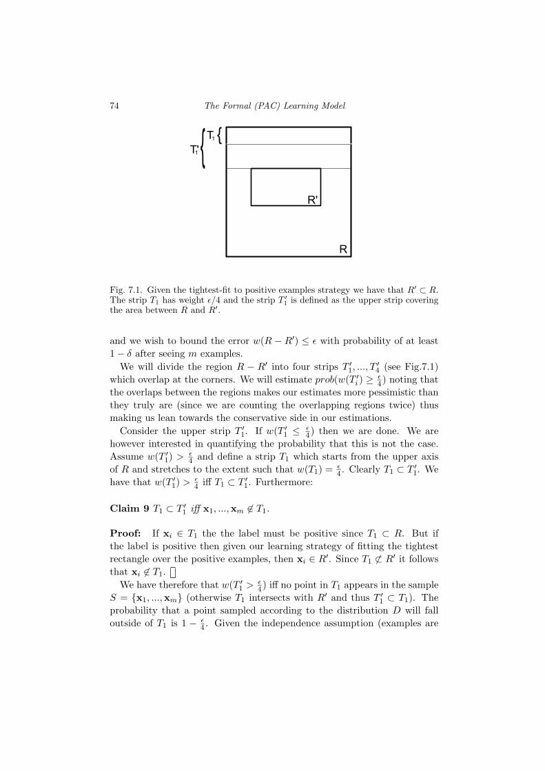
74 The Formal (PAC) Learning Model
Fig. 7.1. Given the tightest-fit to positive examples strategy we have that R′ ⊂ R.The strip T1 has weight ε/4 and the strip T ′
1 is defined as the upper strip coveringthe area between R and R′.
and we wish to bound the error w(R − R′) ≤ ε with probability of at least1− δ after seeing m examples.
We will divide the region R − R′ into four strips T ′1, ..., T′4 (see Fig.7.1)
which overlap at the corners. We will estimate prob(w(T ′i ) ≥ ε4) noting that
the overlaps between the regions makes our estimates more pessimistic thanthey truly are (since we are counting the overlapping regions twice) thusmaking us lean towards the conservative side in our estimations.
Consider the upper strip T ′1. If w(T ′1 ≤ ε4) then we are done. We are
however interested in quantifying the probability that this is not the case.Assume w(T ′1) > ε
4 and define a strip T1 which starts from the upper axisof R and stretches to the extent such that w(T1) = ε
4 . Clearly T1 ⊂ T ′1. Wehave that w(T ′1) > ε
4 iff T1 ⊂ T ′1. Furthermore:
Claim 9 T1 ⊂ T ′1 iff x1, ...,xm 6∈ T1.
Proof: If xi ∈ T1 the the label must be positive since T1 ⊂ R. But ifthe label is positive then given our learning strategy of fitting the tightestrectangle over the positive examples, then xi ∈ R′. Since T1 6⊂ R′ it followsthat xi 6∈ T1.
We have therefore that w(T ′1 >ε4) iff no point in T1 appears in the sample
S = x1, ...,xm (otherwise T1 intersects with R′ and thus T ′1 ⊂ T1). Theprobability that a point sampled according to the distribution D will falloutside of T1 is 1 − ε
4 . Given the independence assumption (examples are

7.3 Learnability of Finite Concept Classes 75
drawn i.i.d.), we have:
prob(x1, ...,xm 6∈ T1) = prob(w(T ′1 >ε
4)) = (1− ε
4)m.
Repeating the same analysis to regions T ′2, T′3, T
′4 and using the union bound
P (A ∪ B) ≤ P (A) + P (B) we come to the conclusion that the probabilitythat any of the four strips of R−R′ has weight greater that ε/4 is at most4(1− ε
4)m. In other words,
prob(err(L′) ≥ ε) ≤ 4((1− ε
4)m ≤ δ.
We can make the expression more convenient for manipulation by using theinequality e−x ≥ 1 − x (recall that 1 + (1/n))n < e from which it followsthat (1 + z)1/z < e and by taking the power of rz where r ≥ 0 we obtain(1 + z)r < erz then set r = 1, z = −x):
4(1− ε
4)m ≤ 4e−
εm4 ≤ δ,
from which we obtain the bound:
m ≥ 4ε
ln4δ.
To conclude, assuming that the learner adopts the tightest-fit to positive ex-amples strategy and is given at least m0 = 4
ε ln 4δ training examples in order
to find the axes-aligned rectangle R′, we can assert that with probability1 − δ the error associated with R′ (i.e., the probability that an (m + 1)’thpoint will be classified incorrectly) is at most ε.
We can see form the analysis above that indeed it applies to any distri-bution D where the only assumption we had to make is the independenceof the draw. Also, the sample size m behaves well in the sense that if onedesires a higher level of accuracy (smaller ε) or a higher level of confidence(smaller δ) then the sample size grows accordingly. The growth of m islinear in 1/ε and linear in ln(1/δ).
7.3 Learnability of Finite Concept Classes
In the previous section we illustrated the concept of learnability with aparticular simple example. We will now focus on applying the learnabilitymodel to a more general family of learning examples. We will consider thefamily of all learning problems over finite concept classes |C| < ∞. Forexample, the conjunction learning problem (over boolean formulas) with n
literals contains only 3n hypotheses because each variable can appear inthe conjunction or not and if appears it could be negated or not. We have

76 The Formal (PAC) Learning Model
shown that n is the lower bound on the number of mistakes on the worstcase analysis any on-line algorithm can achieve. With the definitions wehave above on the formal model of learnability we can perform accuracyand sample complexity analysis that will apply to any learning problemover finite concept classes. This was first introduced by Valiant in 1984.
In the realizable case over |C| < ∞, we will show that any algorithm L
which returns a hypothesis h ∈ C which is consistent with the training setZ is a learning algorithm for C. In other words, any finite concept classis learnable and the learning algorithms simply need to generate consistenthypotheses. The sample complexity m0 associated with the choice of ε andδ can be shown as equal to: 1
ε ln |C|δ .In the unrealizable case, any algorithm L that generates a hypothesis
h ∈ C that minimizes the empirical error (the error obtained on Z) is alearning algorithm for C. The sample complexity can be shown as equal to:2ε2
ln 2|C|δ . We will derive these two cases below.
7.3.1 The Realizable Case
Let h ∈ C be some consistent hypothesis with the training set Z (we knowthat such a hypothesis exists, in particular h = ct the target concept usedfor generating Z) and suppose that
err(h) = prob[x ∼ D : h(x) 6= ct(x)] > ε.
Then, the probability (with respect to the product distribution Dm) that hagrees with ct on a random sample of length m is at most (1 − ε)m. Usingthe inequality we saw before e−x ≥ 1− x we have:
prob[err(h) > ε && h(xi) = ct(xi), i = 1, ...,m] ≤ (1− ε)m < e−εm.
We wish to bound the error uniformly , i.e., that err(h) ≤ ε for all conceptsh ∈ C. This requires the evaluation of:
prob[maxh∈Cerr(h) > ε && h(xi) = ct(xi), i = 1, ...,m].
There at most |C| such functions h, therefore using the Union-Bound theprobability that some function in C has error larger than ε and is consistent

7.3 Learnability of Finite Concept Classes 77
with ct on a random sample of length m is at most |C|e−εm:
prob[∃h : err(h) > ε && h(xi) = ct(xi), i = 1, ...,m]
≤∑
h:err(h)>ε
prob[h(xi) = ct(xi), i = 1, ...,m]
≤ |h : err(h) > ε|e−εm
≤ |C|e−εm
For any positive δ, this probability is less than δ provided:
m ≥ 1ε
ln|C|δ.
This derivation can be summarized in the following theorem (Anthony &Bartlett [1], pp. 25):
Theorem 5 Let C be a finite set of functions from X to Y . Let L bean algorithm such that for any m and for any ct ∈ C, if Z is a trainingsample (xi, ct(xi)), i = 1, ...,m, then the hypothesis h = L(Z) satisfiesh(xi) = ct(xi). Then L is a learning algorithm for C in the realizable casewith sample complexity
m0 =1ε
ln|C|δ.
7.3.2 The Unrealizable Case
In the realizable case an algorithm simply needs to generate a consistenthypothesize to be considered a learning algorithm in the formal sense. Inthe unrealizable situation (a target function ct might not exist) an algorithmwhich minimizes the empirical error, i.e., an algorithm L generates h = L(Z)having minimal sample error:
ˆerr(L(Z)) = minh∈C
ˆerr(h)
is a learning algorithm for C (assuming finite |C|). This is a particularlyuseful property given that the true errors of the functions in C are un-known. It seems natural to use the sample errors ˆerr(h) as estimates to theperformance of L.
The fact that given a large enough sample (training set Z) then the sam-ple error ˆerr(h) becomes close to the true error err(h) is somewhat of arestatement of the ”law of large numbers” of probability theory. For ex-ample, if we toss a coin many times then the relative frequency of ’heads’approaches the true probability of ’head’ at a rate determined by the law of
78 The Formal (PAC) Learning Model
large numbers. We can bound the probability that the difference betweenthe empirical error and the true error of some h exceeds ε using Hoeffding’sinequality:
Claim 10 Let h be some function from X to Y = 0, 1. Then
prob[| ˆerr(h)− err(h)| ≥ ε] ≤ 2e(−2ε2m),
for any probability distribution D, any ε > 0 and any positive integer m.
Proof: This is a straightforward application of Hoeffding’s inequality toBernoulli variables. Hoeffding’s inequality says: Let X be a set, D a proba-bility distribution on X, and f1, ..., fm real-valued functions fi : X → [ai, bi]from X to an interval on the real line (ai < bi). Then,
prob
[| 1m
m∑i=1
fi(xi)− Ex∼D[f(x)]| ≥ ε
]≤ 2e
− 2ε2m2Pi(bi−ai)2 (7.1)
where
Ex∼D[f(x)] =1m
m∑i=1
∫fi(x)D(x)dx.
In our case fi(xi) = 1 iff h(xi) 6= yi and ai = 0, bi = 1. Therefore(1/m)
∑i fi(xi) = ˆerr(h) and err(h) = Ex∼D[f(x)].
The Hoeffding bound almost does what we need, but not quite so. Whatwe have is that for any given hypothesis h ∈ C, the empirical error isclose to the true error with high probability. Recall that our goal is tominimize err(h) over all possible h ∈ C but we can access only ˆerr(h). Ifwe can guarantee that the two are close to each other for every h ∈ C, thenminimizing ˆerr(h) over all h ∈ C will approximately minimize err(h). Putformally, in order to ensure that L learns the class C, we must show that
prob
[maxh∈C| ˆerr(h)− err(h)| < ε
]> 1− δ
In other words, we need to show that the empirical errors converge (at highprobability) to the true errors uniformly over C as m→∞. If that can beguaranteed, then with (high) probability 1− δ, for every h ∈ C,
err(h)− ε < ˆerr(h) < err(h) + ε.
So, since the algorithm L running on training set Z returns h = L(Z) whichminimizes the empirical error, we have:
err(L(Z)) ≤ ˆerr(L(Z)) + ε = minh
ˆerr(h) + ε ≤ Opt(C) + 2ε,

7.3 Learnability of Finite Concept Classes 79
which is what is needed in order that L learns C. Thus, what is left is toprove the following claim:
Claim 11
prob
[maxh∈C| ˆerr(h)− err(h)| ≥ ε
]≤ 2|C|e−2ε2m
Proof: We will use the union bound. Finding the maximum over C isequivalent to taking the union of all the events:
prob
[maxh∈C| ˆerr(h)− err(h)| ≥ ε
]= prob
[⋃h∈CZ : | ˆerr(h)− err(h)| ≥ ε
],
using the union-bound and Claim 2, we have:
≤∑h∈C
prob [| ˆerr(h)− err(h)| ≥ ε] ≤ |C|2e(−2ε2m).
Finally, given that 2|C|e−2ε2m ≤ δ we obtain the sample complexity:
m0 =2ε2
ln2|C|δ.
This discussion is summarized with the following theorem (Anthony & Bartlett[1], pp. 21):
Theorem 6 Let C be a finite set of functions from X to Y = 0, 1. Let Lbe an algorithm such that for any m and for any training set Z = (xi, yi),i = 1, ...,m, then the hypothesis L(Z) satisfies:
ˆerr(L(Z)) = minh∈C
ˆerr(h).
Then L is a learning algorithm for C with sample complexity m0 = 2ε2
ln 2|C|δ .
Note that the main difference with the realizable case (Theorem 1) is thelarger 1/ε2 rather than 1/ε. The realizable case requires a smaller trainingset since we are estimating a random quantity so the smaller the variancethe less data we need.

8
The VC Dimension
The result of the PAC model (also known as the ”formal” learning model)is that if the concept class C is PAC-learnable then the learning strategymust simply consist of gathering a sufficiently large training sample S ofsize m > mo(ε, δ), for given accuracy ε > 0 and confidence 0 < δ < 1parameters, and finds a hypothesis h ∈ C which is consistent with S. Thelearning algorithm is then guaranteed to have a bounded error err(h) < ε
with probability 1 − δ. The error measurement includes data not seen bythe training phase.
This state of affair also holds (with some slight modifications on the sam-ple complexity bounds) when there is no consistent hypothesis (the unreal-izable case). In this case the learner simply needs to minimize the empiricalerror ˆerr(h) on the sample training data S, and if m is sufficiently largethen the learner is guaranteed to have err(h) < Opt(C) + ε with probability1− δ. The measure Opt(C) is defined as the minimal err(g) over all g ∈ C.Note that in the realizable case Opt(C) = 0.
The property of bounding the true error err(h) by minimizing the sampleerror ˆerr(h) is very convenient. The fundamental question is under whatconditions this type of generalization property applies? We saw in the previ-ous lecture that a satisfactorily answer can be provided when the cardinalityof the concept space is bounded, i.e. |C| < ∞, which happens for Booleanconcept space for example. In that lecture we have proven that:
mo(ε, δ) = O(1ε
ln|C|δ
),
is sufficient for guaranteeing a learning model in the formal sense, i.e., whichhas the generalization property described above.
In this lecture and the one that follows we have two goals in mind. Firstis to generalize the result of finite concept class cardinality to infinite car-
80

8.1 The VC Dimension 81
dinality — note that the bound above is not meaningful when |C| = ∞.Can we learn in the formal sense any non-trivial infinite concept class? (wealready saw an example of a PAC-learnable infinite concept class which isthe class of axes aligned rectangles). In order to answer this question we willneed to a general measure of concept class complexity which will replace thecardinality term |C| in the sample complexity bound mo(ε, δ). It is temptingto assume that the number of parameters which fully describe the conceptsof C can serve as such a measure, but we will show that in fact one needsa more powerful measure called the Vapnik-Chervonenkis (VC) dimension.Our second goal is to pave the way and provide the theoretical foundationfor the large margin principle algorithm (SVM) we derived in Lecture 4.
8.1 The VC Dimension
The basic principle behind the VC dimension measure is that although C
may have infinite cardinality, the restriction of the application of conceptsin C to a finite sample S has a finite outcome. This outcome is typicallygoverned by an exponential growth with the size m of the sample S — butnot always. The point at which the growth stops being exponential is whenthe ”complexity” of the concept class C has exhausted itself, in a mannerof speaking.
We will assume C is a concept class over the instance space X — bothof which can be infinite. We also assume that the concept class maps in-stances in X to 0, 1, i.e., the input instances are mapped to ”positive”or ”negative” labels. A training sample S is drawn i.i.d according to somefixed but unknown distribution D and S consists of m instances x1, ...,xm.In our notations we will try to reserve c ∈ C to denote the target conceptand h ∈ C to denote some concept. We begin with the following definition:
Definition 2
ΠC(S) = (h(x1), ..., h(xm) : h ∈ C
which is a set of vectors in 0, 1m.
ΠC(S) is set whose members are m-dimensional Boolean vectors induced byfunctions of C. These members are often called dichotomies or behaviors onS induced or realized by C. If C makes a full realization then ΠC(S) willhave 2m members. An equivalent description is a collection of subsets of S:
ΠC(S) = h ∩ S : h ∈ C
where each h ∈ C makes a partition of S into two sets — the positive and

82 The VC Dimension
negative points. The set ΠC(S) contains therefore subsets of S (the positivepoints of S under h). A full realization will provide
∑mi=0
(mi
)= 2m. We
will use both descriptions of ΠC(S) as a collection of subsets of S and as aset of vectors interchangeably.
Definition 3 If |ΠC(S)| = 2m then S is considered shattered by C. Inother words, S is shattered by C if C realizes all possible dichotomies of S.
Consider as an example a finite concept class C = c1, ..., c4 applied tothree instance vectors with the results:
x1 x2 x3
c1 1 1 1c2 0 1 1c3 1 0 0c4 0 0 0
Then,
ΠC(x1) = (0), (1) shatteredΠC(x1,x3) = (0, 0), (0, 1), (1, 0), (1, 1) shatteredΠC(x2,x3) = (0, 0), (1, 1) not shattered
With these definitions we are ready to describe the measure of concept classcomplexity.
Definition 4 (VC dimension) The VC dimension of C, noted as V Cdim(C),is the cardinality d of the largest set S shattered by C. If all sets S (arbi-trarily large) can be shattered by C, then V Cdim(C) =∞.
V Cdim(C) = maxd | ∃|S| = d, and |ΠC(S)| = 2d
The VC dimension of a class of functions C is the point d at which allsamples S with cardinality |S| > d are no longer shattered by C. As long asC shatters S it manifests its full ”richness” in the sense that one can obtainfrom S all possible results (dichotomies). Once that ceases to hold, i.e.,when |S| > d, it means that C has ”exhausted” its richness (complexity).An infinite VC dimension means that C maintains full richness for all samplesizes. Therefore, the VC dimension is a combinatorial measure of a functionclass complexity.
Before we consider a number of examples of geometric concept classesand their VC dimension, it is important clarify the lower and upper bounds(existential and universal quantifiers) in the definition of VC dimension.The VC dimension is at least d if there exists some sample |S| = d which is

8.1 The VC Dimension 83
shattered by C — this does not mean that all samples of size d are shatteredby C. Conversely, in order to show that the VC dimension is at most d,one must show that no sample of size d+ 1 is shattered. Naturally, provingan upper bound is more difficult than proving the lower bound on the VCdimension. The following examples are shown in a ”hand waiving” styleand are not meant to form rigorous proofs of the stated bounds — they areshown for illustrative purposes only.
Intervals of the real line: The concept class C is governed by two param-eters α1, α2 in the closed interval [0, 1]. A concept from this class will tag aninput instance 0 < x < 1 as positive if α1 ≤ x ≤ α2 and negative otherwise.The VC dimension is at least 2: select a sample of 2 points x1, x2 positionedin the open interval (0, 1). We need to show that there are values of α1, α2
which realize all the possible four dichotomies (+,+), (−,−), (+,−), (−,+).This is clearly possible as one can place the interval [α1, α2] such the inter-section with the interval [x1, x2] is null, (thus producing (−,−)), or to fullyinclude [x1, x2] (thus producing (+,+)) or to partially intersect [x1, x2] suchthat x1 or x2 are excluded (thus producing the remaining two dichotomies).To show that the VC dimension is at most 2, we need to show that anysample of three points x1, x2, x3 on the line (0, 1) cannot be shattered. It issufficient to show that one of the dichotomies is not realizable: the labeling(+,−,+) cannot be realizable by any interval [α1, α2] — this is because ifx1, x3 are labeled positive then by definition the interval [α1, α2] must fullyinclude the interval [x1, x3] and since x1 < x2 < x3 then x2 must be labeledpositive as well. Thus V Cdim(C) = 2.
Axes-aligned rectangles in the plane: We have seen this concept classin the previous lecture — a point in the plane is labeled positive if it liesin an axes-aligned rectangle. The concept class C is thus governed by 4parameters. The VC dimension is at least 4: consider a configuration of4 input points arranged in a cross pattern (recall that we need only toshow some sample S that can be shattered). We can place the rectangles(concepts of the class C) such that all 16 dichotomies can be realized (forexample, placing the rectangle to include the vertical pair of points andexclude the horizontal pair of points would induce the labeling (+,−,+,−)).It is important to note that in this case, not all configurations of 4 pointscan be shattered — but to prove a lower bound it is sufficient to showthe existence of a single shattered set of 4 points. To show that the VCdimension is at most 4, we need to prove that any set of 5 points cannot

84 The VC Dimension
be shattered. For any set of 5 points there must be some point that is”internal”, i.e., is neither the extreme left, right, top or bottom point of thefive. If we label this internal point as negative and the remaining 4 points aspositive then there is no axes-aligned rectangle (concept) which cold realizethis labeling (because if the external 4 points are labeled positive then theymust be fully within the concept rectangle, but then the internal point mustalso be included in the rectangle and thus labeled positive as well).
Separating hyperplanes: Consider first linear half spaces in the plane.The lower bound on the VC dimension is 3 since any three (non-collinear)points in R2 can be shattered, i.e., all 8 possible labelings of the three pointscan be realized by placing a separating line appropriately. By having oneof the points on one side of the line and the other two on the other side wecan realize 3 dichotomies and by placing the line such that all three pointsare on the same side will realize the 4th. The remaining 4 dichotomies arerealized by a sign flip of the four previous cases. To show that the upperbound is also 3, we need to show that no set of 4 points can be shattered.We consider two cases: (i) the four points form a convex region, i.e., lie onthe convex hull defined by the 4 points, (ii) three of the 4 points define theconvex hull and the 4th point is internal. In the first case, the labeling whichis positive for one diagonal pair and negative to the other pair cannot berealized by a separating line. In the second case, a labeling which is positivefor the three hull points and negative for the interior point cannot be realize.Thus, the VC dimension is 3 and in general the VC dimension for separatinghyperplanes in Rn is n+ 1.
Union of a finite number of intervals on the line: This is an exampleof a concept class with an infinite VC dimension. For any sample of pointson the line, one can place a sufficient number of intervals to realize anylabeling.
The examples so far were simple enough that one might get the wrongimpression that there is a correlation between the number of parametersrequired to describe concepts of the class and the VC dimension. As acounter example, consider the two parameter concept class:
C = sign(sin(ωx+ θ) : ω
which has an infinite VC dimension as one can show that for every setof m points on the line one can realize all possible labelings by choosing
8.2 The Relation between VC dimension and PAC Learning 85
a sufficiently large value of ω (which serves as the frequency of the syncfunction) and appropriate phase.
We conclude this section with the following claim:
Theorem 7 The VC dimension of a finite concept class |C| <∞ is boundedfrom above:
V Cdim(C) ≤ log2 |C|.
Proof: if V Cdim(C) = d then there exists at least 2d functions in C
because every function induces a labeling and there are at least 2d labelings.Thus, from |C| ≥ 2d follows that d ≤ log2 |C|.
8.2 The Relation between VC dimension and PAC Learning
We saw that the VC dimension is a combinatorial measure of concept classcomplexity and we would like to have it replace the cardinality term in thesample complexity bound. The first result of interest is to show that ifthe VC dimension of the concept class is infinite then the class is not PAClearnable.
Theorem 8 Concept class C with V Cdim(C) = ∞ is not learnable in theformal sense.
Proof: Assume the contrary that C is PAC learnable. Let L be the learningalgorithm and m be the number of training examples required to learn theconcept class with accuracy ε = 0.1 and 1 − δ = 0.9. That is, after seeingat least m(ε, δ) training examples, the learner generates a concept h whichsatisfies p(err(h) ≤ 0.1) ≥ 0.9.
Since the VC dimension is infinite there exist a sample set S with 2minstances which is shattered by C. Since the formal model (PAC) appliesto any training sample we will use the set S as follows. We will define aprobability distribution on the instance space X which is uniform on S (withprobability 1
2m) and zero everywhere else.Because S is shattered, then any target concept is possible so we will
choose our target concept c in the following manner:
prob(ct(xi) = 0) =12∀xi ∈ S,
in other words, the labels ct(xi) are determined by a coin flip. The learnerL selects an i.i.d. sample of m instances S — which due to the structure of

86 The VC Dimension
D means that the S ⊂ S and outputs a consistent hypothesis h ∈ C. Theprobability of error for each xi 6∈ S is:
prob(ct(xi) 6= h(xi)) =12.
The reason for that is because S is shattered by C, i.e., we can select anytarget concept for any labeling of S (the 2m examples) therefore we couldselect the labels of the m points not seen by the learner arbitrarily (byflipping a coin). Regardless of h, the probability of mistake is 0.5. Theexpectation on the error of h is:
E[err(h)] = m · 0 · 12m
+m · 12· 1
2m=
14.
This is because we have 2m points to sample (according to D as all otherpoints have zero probability) from which the error on half of them is zero(as h is consistent on the training set S) and the error on the remaining halfis 0.5. Thus, the average error is 0.25. Note that E[err(h)] = 0.25 for anychoice of ε, δ as it is based on the sample size m. For any sample size m wecan follow the construction above and generate the learning problem suchthat if the learner produces a consistent hypothesis the expectation of theerror will be 0.25.
The result that E[err(h)] = 0.25 is not possible for the accuracy andconfidence values we have set: with probability of at least 0.9 we have thaterr(h) ≤ 0.1 and with probability 0.1 then err(h) = β where 0.1 < β ≤ 1.Taking the worst case of β = 1 we come up with the average error:
E[err(h)] ≤ 0.9 · 0.1 + 0.1 · 1 = 0.19 < 0.25.
We have therefore arrived to a contradiction that C is PAC learnable.We next obtain a bound on the growth of |ΠS(C)| when the sample size|S| = m is much larger than the VC dimension V Cdim(C) = d of theconcept class. We will need few more definitions:
Definition 5 (Growth function)
ΠC(m) = max|ΠS(C)| : |S| = m
The measure ΠC(m) is the maximum number of dichotomies induced by Cfor samples of size m. As long as m ≤ d then ΠC(m) = 2m. The questionis what happens to the growth pattern of ΠC(m) when m > d. We willsee that the growth becomes polynomial — a fact which is crucial for thelearnability of C.

8.2 The Relation between VC dimension and PAC Learning 87
Definition 6 For any natural numbers m, d we have the following definition:
Φd(m) = Φd(m− 1) + Φd−1(m− 1)
Φd(0) = Φ0(m) = 1
By induction on m, d it is possible to prove the following:
Theorem 9
Φd(m) =d∑i=0
(m
i
)Proof: by induction on m, d. For details see [[3], pp. 56].
For m ≤ d we have that Φd(m) = 2m. For m > d we can derive apolynomial upper bound as follows.(
d
m
)d d∑i=0
(m
i
)≤
d∑i=0
(d
m
)i(mi
)≤
m∑i=0
(d
m
)i(mi
)= (1 +
d
m)m ≤ ed
From which we obtain: (d
m
)dΦd(m) ≤ ed.
Dividing both sides by(dm
)dyields:
Φd(m) ≤ ed(md
)d=(emd
)d= O(md).
We need one more result before we are ready to present the main result ofthis lecture:
Theorem 10 (Sauer’s lemma) If V Cdim(C) = d, then for any m,ΠC(m) ≤ Φd(m).
Proof: By induction on both d,m. For details see [[3], pp. 55–56].Taken together, we have now a fairly interesting characterization on how
the combinatorial measure of complexity of the concept class C scales upwith the sample size m. When the VC dimension of C is infinite the growthis exponential, i.e., ΠC(m) = 2m for all values of m. On the other hand,when the concept class has a bounded VC dimension V Cdim(C) = d < ∞then the growth pattern undergoes a discontinuity from an exponential toa polynomial growth:
ΠC(m) =
2m m ≤ d
≤(emd
)dm > d

88 The VC Dimension
As a direct result of this observation, when m >> d is much larger than d
the entropy becomes much smaller than m. Recall than from an informa-tion theoretic perspective, the entropy of a random variable Z with discretevalues z1, ..., zn with probabilities pi, i = 1, ..., n is defined as:
H(Z) =n∑i=0
pi log2
1pi,
where I(pi) = log21pi
is a measure of ”information”, i.e., is large whenpi is small (meaning that there is much information in the occurrence ofan unlikely event) and vanishes when the event is certain pi = 1. Theentropy is therefore the expectation of information. Entropy is maximal fora uniform distribution H(Z) = log2 n. The entropy in information theorycontext can be viewed as the number of bits required for coding z1, ..., zn. Incoding theory it can be shown that the entropy of a distribution provides thelower bound on the average length of any possible encoding of a uniquelydecodable code fro which one symbol goes into one symbol. When thedistribution is uniform we will need the maximal number of bits, i.e., onecannot compress the data. In the case of concept class C with VC dimensiond, we see that one when m ≤ d all possible dichotomies are realized andthus one will need m bits (as there are 2m dichotomies) for representingall the outcomes of the sample. However, when m >> d only a smallfraction of the 2m dichotomies can be realized, therefore the distributionof outcomes is highly non-uniform and thus one would need much less bitsfor coding the outcomes of the sample. The technical results which followare therefore a formal way of expressing in a rigorous manner this simpletruth — If it is possible to compress, then it is possible to learn. The crucialpoint is that learnability is a direct consequence of the ”phase transition”(from exponential to polynomial) in the growth of the number of dichotomiesrealized by the concept class.
In the next lecture we will continue to prove the ”double sampling” the-orem which derives the sample size complexity as a function of the VCdimension.
9
The Double-Sampling Theorem
In this lecture will use the measure of VC dimension, which is a combina-torial measure of concept class complexity, to bound the sample size com-plexity.
9.1 A Polynomial Bound on the Sample Size m for PAC Learning
In this section we will follow the material presented in Kearns & Vazirani[3] pp. 57–61 and prove the following:
Theorem 11 (Double Sampling) Let C be any concept class of VC di-mension d. Let L be any algorithm that when given a set S of m labeledexamples xi, c(xi)i, sampled i.i.d according to some fixed but unknowndistribution D over the instance space X, of some concept c ∈ C, producesas output a concept h ∈ C that is consistent with S. Then L is a learningalgorithm in the formal sense provided that the sample size obeys:
m ≥ c0
(1ε
log1δ
+d
εlog
1ε
)for some constant c0 > 0.
The idea behind the proof is to build an ”approximate” concept space whichincludes concepts arranged such that the distance between the approximateconcepts h and the target concept c is at least ε — where distance is de-fined as the weight of the region in X which is in conflict with the targetconcept. To formalize this story we will need few more definitions. Unlessspecified otherwise, c ∈ C denotes the target concept and h ∈ C denotessome concept.
89
90 The Double-Sampling Theorem
Definition 7
c∆h = h∆c = x : c(x) 6= h(x)
c∆h is the region in instance space where both concepts do not agree —the error region. The probability that x ∈ c∆h is equal to (by definition)err(h).
Definition 8
∆(c) = h∆c : h ∈ C∆ε(c) = h∆c : h ∈ C and err(h) ≥ ε
∆(c) is a set of error regions, one per concept h ∈ C over all concepts. Theerror regions are with respect to the target concept. The set ∆ε(c) ⊂ ∆(c)is the set of all error regions whose weight exceeds ε. Recall that weight isdefined as the probability that a point sampled according to D will hit theregion.
It will be important for later to evaluate the VC dimension of ∆(c). UnlikeC, we are not looking for the VC dimension of a class of function but theVC dimension of a set of regions in space. Recall the definition of ΠC(S)from the previous lecture: there were two equivalent definitions one basedon a set of vectors each representing a labeling of the instances of S inducedby some concept. The second, yet equivalent, definition is based on a setof subsets of S each induced by some concept (where the concept dividesthe sample points of S into positive and negative labeled points). So far itwas convenient to work with the first definition, but for evaluating the VCdimension of ∆(c) it will be useful to consider the second definition:
Π∆(c)(S) = r ∩ S : r ∈ ∆(c),
that is, the collection of subsets of S induced by intersections with regionsof ∆(c). An intersection between S and a region r is defined as the subset ofpoints from S that fall into r. We can easily show that the VC dimensionsof C and ∆(c) are equal:
Lemma 1
V Cdim(C) = V Cdim(∆(c)).
Proof: we have that the elements of ΠC(S) and Π∆(c)(S) are susbsets ofS, thus we need to show that for every S the cardinality of both sets isequal |ΠC(S)| = |Π∆(c)(S)|. To do that it is sufficient to show that for everyelement s ∈ ΠC(S) there is a unique corresponding element in Π∆(c)(S). Let
9.1 A Polynomial Bound on the Sample Size m for PAC Learning 91
c∩S be the subset of S induced by the target concept c. The set s (a subsetof S) is realized by some concept h (those points in S which were labeledpositive by h). Therefore, the set s ∩ (c ∩ S) is the subset of S containingthe points that hit the region h∆c which is an element of Π∆(c)(S). Sincethis is a one-to-one mapping we have that |ΠC(S)| = |Π∆(c)(S)|.
Definition 9 (ε-net) For every ε > 0, a sample set S is an ε-net for ∆(c)if every region in ∆ε(c) is hit by at least one point of S:
∀r ∈ ∆ε(c), S ∩ r 6= ∅.
In other words, if S hits all the error regions in ∆(c) whose weight exceedsε, then S is an ε-net. Consider as an example the concept class of intervalson the line [0, 1]. A concept is defined by an interval [α1, α2] such that allpoints inside the interval are positive and all those outside are negative.Given c ∈ C is the target concept and h ∈ C is some concept, then theerror region h∆c is the union of two intervals: I1 consists of all points x ∈ hwhich are not in c, and I2 the interval of all points x ∈ c but which are notin h. Assume that the distribution D is uniform (just for the sake of thisexample) then, prob(x ∈ I) = |I| which is the length of the interval I. As aresult, err(h) > ε if either |I1| > ε/2 or |I2| > ε/2. The sample set
S = x =kε
2: k = 0, 1, ..., 2/ε
contains sample points from 0 to 1 with increments of ε/2. Therefore, everyinterval larger than ε must be hit by at least one point from S and bydefinition S is an ε-net.
It is important to note that if S forms an ε-net then we are guaranteedthat err(h) ≤ ε. Let h ∈ C be the consistent hypothesis with S (returnedby the learning algorithm L). Becuase h is consistent, h∆c ∈ ∆(c) hasnot been hit by S (recall that h∆c is the error region with respect to thetarget concept c, thus if h is consistent then it agrees with c over S andtherefore S does not hit h∆c). Since S forms an ε-net for ∆(c) we musthave h∆c 6∈ ∆ε(c) (recall that by definition S hits all error regions withweight larger than ε). As a result, the error region h∆c must have a weightsmaller than ε which means that err(h) ≤ ε.
The conclusion is that if we can bound the probability that a random sam-ple S does not form an ε-net for ∆(c), then we have bounded the probabilitythat a concept h consistent with S has err(h) > ε. This is the goal of theproof of the double-sampling theorem which we are about to prove below:

92 The Double-Sampling Theorem
Proof (following Kearns & Vazirani [3] pp. 59–61): Let S1 be a ran-dom sample of size m (sampled i.i.d. according to the unknown distributionD) and let A be the event that S1 does not form an ε-net for ∆(c). Fromthe preceding discussion our goal is to upper bound the probability for A tooccur, i.e., prob(A) ≤ δ.
If A occurs, i.e., S1 is not an ε-net, then by definition there must be someregion r ∈ ∆ε(c) which is not hit by S1, that is S1 ∩ r = ∅. Note thatr = h∆(c) for some concept h which is consistent with S1. At this point thespace of possibilities is infinite, because the probability that we fail to hith∆(c) in m random examples is at most (1− ε)m. Thus the probability thatwe fail to hit some h∆c ∈ ∆ε(c) is bounded from above by |∆(c)|(1 − ε)m— which does not help us due to the fact that |∆(c)| is infinite. The ideaof the proof is to turn this into a finite space by using another sample, asfollows.
Let S2 be another random sample of size m. We will select m (for bothS1 and S2) to guarantee a high probability that S2 will hit r many times.In fact we wish that S2 will hit r at least εm
2 with probability of at least 0.5:
prob(|S2 ∩ r| >εm
2) = 1− prob(|S2 ∩ r| ≤
εm
2).
We will use the Chernoff bound (lower tail) to obtain a bound on the right-hand side term. Recall that if we have m Bernoulli trials (coin tosses)Z1, ..., Zm with expectation E(Zi) = p and we consider the random variableZ = Z1 + ...+ Zm with expectation E(Z) = µ (note that µ = pm) then forall 0 < ψ < 1 we have:
prob(Z < (1− ψ)µ) ≤ e−µψ2
2 .
Considering the sampling of m examples that form S2 as Bernoulli trials,we have that µ ≥ εm (since the probability that an example will hit r is atleast ε) and ψ = 0.5. We obtain therefore:
prob(|S2 ∩ r| ≤ (1− 12
)εm) ≤ e−εm8 =
12
which happens when m = 8ε ln 2 = O(1
ε ). To summarize what we haveobtained so far, we have calculated the probability that S2 will hit r manytimes given that r was fixed using the previous sampling, i.e., given that S1
does not form an ε-net. To formalize this, let B denote the combined eventthat S1 does not form an ε-event and S2 hits r at least εm/2 times. Then,we have shown that for m = O(1/ε) we have:
prob(B/A) ≥ 12.
9.1 A Polynomial Bound on the Sample Size m for PAC Learning 93
From this we can calculate prob(B):
prob(B) = prob(B/A)prob(A) ≥ 12prob(A),
which means that our original goal of bounding prob(A) is equivalent tofinding a bound prob(B) ≤ δ/2 because prob(A) ≤ 2 · prob(B) ≤ δ. Thecrucial point with the new goal is that to analyze the probability of theevent B, we need only to consider a finite number of possibilities, namely toconsider the regions of
Π∆ε(c)(S1 ∪ S2) = r ∩ S1 ∪ S2 : r ∈ ∆ε(c) .
This is because the occurrence of the event B is equivalent to saying thatthere is some r ∈ Π∆ε(c)(S1 ∪ S2) such that |r| ≥ εm/2 (i.e., the region r
is hit at least εm/2 times) and S1 ∩ r = ∅. This is because Π∆ε(c)(S1 ∪ S2)contains all the subsets of S1 ∪ S2 realized as intersections over all regionsin ∆ε(c). Thus even though we have an infinite number of regions we stillhave a finite number of subsets. We wish therefore to analyze the followingprobability:
prob(r ∈ Π∆ε(c)(S1 ∪ S2) : |r| ≥ εm/2 and S1 ∩ r = ∅
).
Let S = S1∪S2 a random sample of 2m (note that since the sampling is i.i.d.it is equivalent to sampling S1 and S2 separately) and r satisfying |r| ≥ εm/2being fixed. Consider some random partitioning of S into S1 and S2 andconsider then the problem of estimating the probability that S1 ∩ r = ∅.This problem is equivalent to the following combinatorial question: we have2m balls, each colored Red or Blue, with exaclty l ≥ εm/2 Red balls. Wedivide the 2m balls into groups of equal size S1 and S2 and we are interestedin bounding the probability that all of the l balls fall in S2 (that is, theprobability that S1 ∩ r = ∅). This in turn is equivalent to first dividing the2m uncolored balls into S1 and S2 groups and then randomly choose l ofthe balls to be colored Red and analyze the probability that all of the Redballs fall into S2. This probability is exactly(
ml
)(2ml
) =l−1∏i=0
m− i2m− i
≤l−1∏i=0
12
=12l
= 2−εm/2.
This probability was evaluated for a fixed S and r. Thus, the probability thatthis occurs for some r ∈ Π∆ε(c)(S) satisfying |r| ≥ εm/2 (which is prob(B))can be calculated by summing over all possible fixed r and applying the
94 The Double-Sampling Theorem
union bound prob(∑
i Zi) ≤∑
i prob(Zi):
prob(B) ≤ |Π∆ε(c)(S)|2−εm/2 ≤ |Π∆(c)(S)|2−εm/2
= |ΠC(S)|2−εm/2 ≤(
2εmd
)d2−εm/2 ≤ δ
2,
from which it follows that:
m = O
(1ε
log1δ
+d
εlog
1ε
).
Few comments are worthwhile at this point:
(i) It is possible to show that the upper bound on the sample complexitym is tight by showing that the lower bound on m is Ω(d/ε) (see [[3],pp. 62]).
(ii) The treatment above holds also for the unrealizable case (target con-cept c 6∈ C) with slight modifications to the bound. In this context,the learning algorithm L must simply minimize the sample (empiri-cal) error ˆerr(h) defined:
ˆerr(h) =1m|i : h(xi) 6= yi| xi ∈ S.
The generalization of the double-sampling theorem (Derroye’82) statesthat the empirical errors converge uniformly to the true errors:
prob
(maxh∈C| ˆerr(h)− err(h)| ≥ ε
)≤ 4e(4ε+4ε2)
(εm2
d
)d2−mε
2/2 ≤ δ,
from which it follows that
m = O
(1ε2
log1δ
+d
ε2log
1ε
).
Taken together, we have arrived to a fairly remarkable result. Despite thefact that the distribution D from which the training sample S is drawn fromis unknown (but is known to be fixed), the learner simply needs to minimizethe empirical error. If the sample size m is large enough the learner is guar-anteed to have minimized the true errors for some accuracy and confidenceparameters which define the sample size complexity. Equivalently,
|Opt(C)− ˆerr(h)| −→m→∞ 0.
Not only is the convergence is independent of D but also the rate of con-vergence is independent (namely, it does not matter where the optimal h∗

9.2 Optimality of SVM Revisited 95
is located). The latter is very important because without it one could ar-bitrarily slow down the convergence rate by maliciously choosing D. Thebeauty of the results above is that D does not have an effect at all — onesimply needs to choose the sample size to be large enough for the accuracy,confidence and VC dimension of the concept class to be learned over.
9.2 Optimality of SVM Revisited
In Lecture 4 we discussed the large margin principle for finding an optimalseparating hyperplane. It is natural to ask how does the PAC theory pre-sented so far explains why a maximal margin hyperplane is optimal withregard to the formal sense of learning (i.e. to generalization from empiricalerrors to true errors)? We saw in the previous section that the sample com-plexity m(ε, δ, d) depends also on the VC dimension of the concept class —which is n + 1 for hyperplanes in Rn. Thus, another natural question thatmay certainly arise is what is the gain in employing the ”kernel trick”? For afixed m, mapping the input instance space X of dimension n to some higher(exponentially higher) feature space might simply mean that we are compro-mising the accuracy and confidence of the learner (since the VC dimensionis equal to the instance space dimension plus 1).
Given a fixed sample size m, the best the learner can do is to minimize theempirical error and at the same time to try to minimize the VC dimension dof the concept class. The smaller d is, for a fixed m, the higher the accuracyand confidence of the learning algorithm. Likewise, the smaller d is, for afixed accuracy and confidence values, the smaller sample size is required.
There are two possible ways to decrease d. First is to decrease the dimen-sion n of the instance space X. This amounts to ”feature selection”, namelyfind a subset of coordinates that are the most ”relevant” to the learningtask r perform a dimensionality reduction via PCA, for example. A secondapproach is to maximize the margin. Let the margin associated with theseparating hyperplane h (i.e. consistent with the sample S) be γ. Let theinput vectors x ∈ X have a bounded norm, |x| ≤ R. It can be shown thatthe VC dimension of the concept class Cγ of hyperplanes with margin γ is:
Cγ = minR2
γ2, n
+ 1.
Thus, if the margin is very small then the VC dimension remains n+ 1. Asthe margin gets larger, there comes a point where R2/γ2 < n and as a resultthe VC dimension decreases. Moreover, mapping the instance space X tosome higher dimension feature space will not change the VC dimension as

96 The Double-Sampling Theorem
long as the margin remains the same. It is expected that the margin will notscale down or will not scale down as rapidly as the scaling up of dimensionfrom image space to feature space.
To conclude, maximizing the margin (while minimizing the empirical er-ror) is advantageous as it decreases the VC dimension of the concept classand causes the accuracy and confidence values of the learner to be largelyimmune to dimension scaling up while employing the kernel trick.

10
Appendix
97

98 Appendix
A0.1 Variance, Covariance, etc.
Let X,Y be two random variables and let f(x, y) be some function on x ∈X, y ∈ Y , and let p(x, y) be the probability of the event x and y occurringtogether. The expectation E[f(x, y)] is defined:
E[f(x, y)] =∑x∈X
∑y∈Y
f(x, y)p(x, y)
. The mean, variance and covariance are defined:
µx = E[X] =∑x
∑y
xp(x, y)
µy = E[Y ] =∑x
∑y
yp(x, y)
σ2x = V ar[X] = E[(x− µx)2] =
∑x
∑y
(x− µx)2p(x, y)
σ2y = V ar[Y ] = E[(y − µy)2] =
∑x
∑y
(y − µy)2p(x, y)
σxy = Cov(XY ) = E[(x− µx)(y − µy)] =∑x
∑y
(x− µx)(y − µy)p(x, y)
In vector-matrix notation, let x represent the n random variables ofX1, ..., Xn,i.e., x = (x1, ..., xn)> is an instance vector and p(x) is the probability of theinstance occurrence. Then the mean is a vector µ and the covariance matrixE are defined:
µ =∑
x∈X1,...,Xn
xp(x)
E =∑x
(x− µ)(x− µ)>p(x)
Note that the covariance matrix E is the linear superposition of rank-1matrices (x−µ)(x−µ)> with coefficients p(x). The diagonal of E containesthe variances of the variables x1, ..., xn. For a uniform distribution anda sample data S consisting of m points, let A = [x1 − µ, ...,xm − µ] bethe matrix whose columns consist of the points centered around the mean:µ = 1
m
∑i xi. The (sample) covariance matrix is E = 1
mAA>.

A0.2 Derivatives of Matrix Operations: Scalar Functions of a Vector 99
A0.2 Derivatives of Matrix Operations: Scalar Functions of aVector
The two most important examples of a scalar function of a vector x are thelinear form a>x and the quadratic form x>Ax for some square matrix A.
d(a>x) = a>dx
d(x>Ax) = (dx)>Ax + x>A(dx)
=(
(dx)>Ax)>
+ x>A(dx)
= x>(A+A>)dx
where the derivative d(x>Ax) using the rule of products d(f · g) = (df) · g+f · (dg) where g = Ax and f = x> and noting that d(Ax) = Adx. Thus,ddx(a>x) = a> and d
dx(x>Ax)) = x>(A + A>). If A is symmetric thenddx(x>Ax)) = (2Ax)>.
A0.3 Primer on Constrained Optimization
A0.3.1 Equality Constraints and Lagrange Multipliers
Consider first the general optimization with equality constraints which givesrise to the notion of Lagrange multipliers.
minx
f(x) (0.1)
subject to
h(x) = 0
where f : Rn → R and h : Rn → Rk where h is a vector function (h1, ..., hk)each from Rn to R. We want to derive a necessary and sufficient constraintfor a point xo to be a local minimum subject to the k equality constraintsh(x) = 0. Assume that xo is a regular point, meaning that the gradientvectors ∇hj(x) are linearly independent. Note that ∇h(xo) is a k×n matrixand the null space of this matrix:
null(∇h(xo)) = y : ∇h(xo)y = 0
defines the tangent plane at the point xo. We have the following fundamentaltheorem:
∇f(xo) ⊥ null(∇h(xo))
in other words, all vectors y spanning the tangent plane at the point xo arealso perpendicular to the gradient of f at xo.
100 Appendix
The sketch of the proof is as follows. Let x(t), −a ≤ t < a, be a smoothcurve on the surface h(x) = 0, i.e., h(x(t)) = 0. Let xo = x(0) and y =ddtx(0) the tangent to the curve at xo. From the definition of tangency, thevector y lives in null(∇h(xo)), i.e., y · ∇hj(x(0)) = 0, j = 1, ..., k. Sincexo = x(0) is a local extremum of f(x), then
0 =d
dtf(x(t))|t=0 =
∑ ∂f
∂xi
dxidt|t=0 = ∇f(xo) · y.
As a corollary of this basic theorem, the gradient vector∇f(xo) ∈ span∇h1(xo), ...,∇hk(xo),i.e.,
∇f(xo) +k∑i=1
λi∇hi(xo) = 0,
where the coefficients λi are called Lagrange Multipliers and the expression:
f(x) +∑i
λihi(x)
is called the Lagrangian of the optimization problem (0.1).
A0.3.2 Inequality Constraints and KKT conditions
Consider next the general constrained optimization with inequality con-straints (called “non-linear programming”):
minx
f(x) (0.2)
subject to
h(x) = 0
g(x) ≤ 0
where g : Rn → Rs. We will assume that the optimal solution xo is aregular point which has the following meaning: Let J be the set of indicesj such that gj(xo) = 0, then xo is a regular point if the gradient vectors∇hi(xo),∇gj(xo), i = 1, ..., k and j ∈ J are linearly independent. A basicresult (we will not prove here) is the Karush-Kuhn-Tucker (KKT) theorem:
Let xo be a local minimum of the problem and suppose xo is a regularpoint. Then, there exist λ1, ..., λk and µ1 ≥ 0, ..., µs ≥ 0 such that:

A0.3 Primer on Constrained Optimization 101
),( ** zy
),( zy
y
z
!µ =+ yzG
nRx"))(),(( xfxg
)(µ#
Fig. A0.1. Geometric interpreatation of Duality (see text).
∇f(xo) +k∑i=1
λi∇hi(xo) +s∑j=1
µj∇gj(xo) = 0, (0.3)
s∑j=1
µjgj(xo) = 0. (0.4)
Note that the condition∑µjgj(xo) = 0 is equivalent to the condition that
µjgj(xo) = 0 (since µ ≥ 0 and g(xo) ≤ 0 thus there sum cannot vanishunless each term vanishes) which in turn implies: µj = 0 when gj(xo) < 0.The expression
L(x, λ, µ) = f(x) +k∑i=1
λihi(x) +s∑j=1
µjgj(x)
is the Lagrangian of the problem (0.2) and the associated condition µjgj(xo) =0 is called the KKT condition.
The remaining concepts we need are the “duality” and the “LagrangianDual” problem.

102 Appendix
A0.3.3 The Langrangian Dual Problem
The optimization problem (0.2) is called the “Primal” problem. The La-grangian Dual problem is defined as:
maxλ,µ
θ(λ, µ) (0.5)
subject to
µ ≥ 0 (0.6)
where
θ(λ, µ) = minxf(x) +
∑i
λihi(x) +∑j
µjgj(x).
Note that θ(λ, µ) may assume the value −∞ for some values of λ, µ (thusto be rigorous we should have replaced “min” with “inf”). The first basicresult is the weak duality theorem:
Let x be a feasible solution to the primal (i.e., h(x) = 0,g(x) ≤ 0) and let(λ, µ) be a feasible solution to the dual problem (i.e., µ ≥ 0), then f(x) ≥θ(λ, µ)
The proof is immediate:
θ(λ, µ) = minyf(y) +
∑i
λihi(y) +∑j
µjgj(y)
≤ f(x) +∑i
λihi(x) +∑j
µjgj(x)
≤ f(x)
where the latter inequality follows from h(x) = 0 and∑
j µjgj(x) ≤ 0because µ ≥ 0 and g(x) ≤ 0. As a corollary of this theorem we have:
minxf(x) : h(x) = 0,g(x) ≤ 0 ≥ max
λ,µθ(λ, µ) : µ ≥ 0. (0.7)
The next basic result is the strong duality theorem which specifies the con-ditions for when the inequality in (0.7) becomes equality:
Let f(),g() be convex functions and let h() be affine, i.e., h(x) = Ax−bwhere A is a k × n matrix, then
minxf(x) : h(x) = 0,g(x) ≤ 0 = max
λ,µθ(λ, µ) : µ ≥ 0.
The strong duality theorem allows one to solve for the primal problem byfirst dualizing it and solving for the dual problem instead (we will see exactlyhow to do it when we return to solving the primal problem (4.3)). When
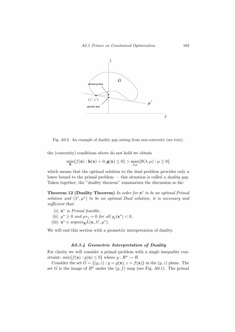
A0.3 Primer on Constrained Optimization 103
),( ** zy
y
z
G
*µ
optimal primal
optimal dual
Fig. A0.2. An example of duality gap arising from non-convexity (see text).
the (convexity) conditions above do not hold we obtain
minxf(x) : h(x) = 0,g(x) ≤ 0 > max
λ,µθ(λ, µ) : µ ≥ 0
which means that the optimal solution to the dual problem provides only alower bound to the primal problem — this situation is called a duality gap.Taken together, the ”duality theorem” summarizes the discussion so far:
Theorem 12 (Duality Theorem) In order for x∗ to be an optimal Primalsolution and (λ∗, µ∗) to be an optimal Dual solution, it is necessary andsufficient that:
(i) x∗ is Primal feasible,(ii) µ∗ ≥ 0 and µ∗j = 0 for all gj(x∗) < 0,(iii) x∗ ∈ argminxL(x, λ∗, µ∗).
We will end this section with a geometric interpretation of duality.
A0.3.4 Geometric Interpretation of Duality
For clarity we will consider a primal problem with a single inequality con-straint: minf(x) : g(x) ≤ 0 where g : Rn → R.
Consider the set G = (y, z) : y = g(x), z = f(x) in the (y, z) plane. Theset G is the image of Rn under the (g, f) map (see Fig. A0.1). The primal

104 Appendix
problem is to find a point in G that has a y ≤ 0 with the smallest z value— this is the point (y∗, z∗) in the figure.
In this case θ(µ) = minxf(x) + µg(x) which is equivalent to minimizez + µy over points in G. The equation z + µy = α represents a straight linewith slope −µ and intercept (on z axis) α. For a given value µ, to minimizez + µy over G we need to move the line z + µy = α parallel to itself as fardown as possible while it remains in contact with G — in other words Gis above the line and touches it. Then, the intercept with the z axis givesθ(µ). The dual problem is therefore equivalent to finding the slope of thesupporting hyperplane such that its intercept on the z axis is maximal.
Consider the non-convex region G in Fig. A0.2 which illustrates a dualitygap condition. The optimal primal is the point (y∗, z∗) which is higher thanthe greatest intercept on the z axis achieved by a line that supports G frombelow. This is an example of a duality gap caused by the non-convexity ofthe functions f(), g() (thereby making the set G non-convex).

Bibliography
M. Anthony and P.L. Bartlett. Neural Neteowk Learning: Theoretical Foundations.Cambridge University Press, 1999.
K.M. Hall. An r-dimensional quadratic placement algorithm. Manag. Sci., 17:219–229, 1970.
M.J. Kearns and U.V. Vazirani. An Introduction to Computational Learning The-ory. MIT Press, 1997.
Y. Linde, A. Buzo, and R.M. Gray. An algorithm for vector quantizer design. IEEETransactions on Communications, 1:84–95, 1980.
A.Y. Ng, M.I. Jordan, and Y. Weiss. On spectral clustering: Analysis and analgorithm. In Proceedings of the conference on Neural Information ProcessingSystems (NIPS), 2001.
J. Shi and J. Malik. Normalized cuts and image segmentation. IEEE Transactionson Pattern Analysis and Machine Intelligence, 22(8), 2000.
R. Zass and A. Shashua. A unifying approach to hard and probabilistic clustering.In Proceedings of the International Conference on Computer Vision, Beijing,China, Oct. 2005.
105