Introduction to Linear Regression and Correlation Analysis

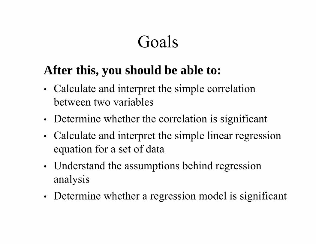
GoalsAfter this, you should be able to:• Calculate and interpret the simple correlation

between two variables• Determine whether the correlation is significant• Calculate and interpret the simple linear regression

equation for a set of data• Understand the assumptions behind regression

analysis• Determine whether a regression model is significant

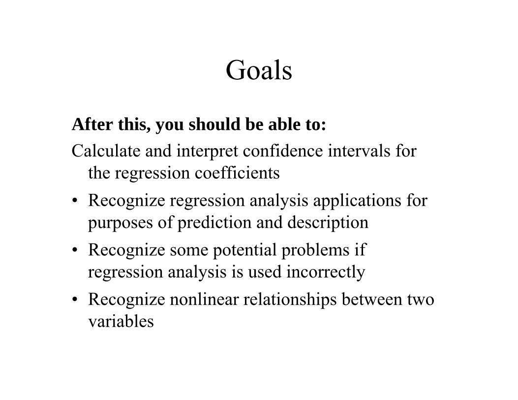
Goals

After this, you should be able to:Calculate and interpret confidence intervals for

the regression coefficients• Recognize regression analysis applications for

purposes of prediction and description• Recognize some potential problems if

regression analysis is used incorrectly• Recognize nonlinear relationships between two

variables

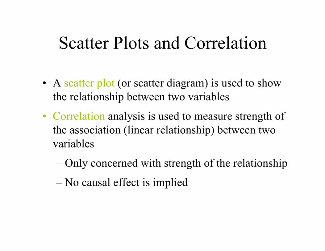
Scatter Plots and Correlation

• A scatter plot (or scatter diagram) is used to show the relationship between two variables

• Correlation analysis is used to measure strength of the association (linear relationship) between two variables

– Only concerned with strength of the relationship

– No causal effect is implied

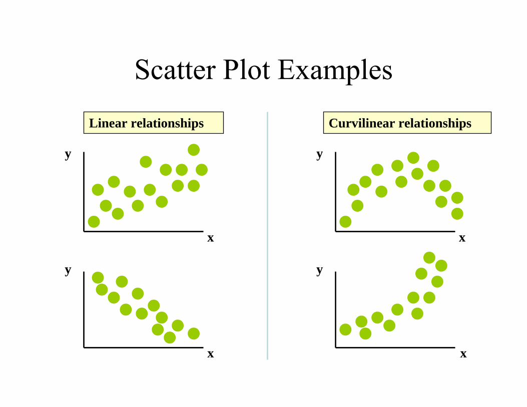
Scatter Plot Examples

y

x

y

x

y

y

x

x

Linear relationships Curvilinear relationships

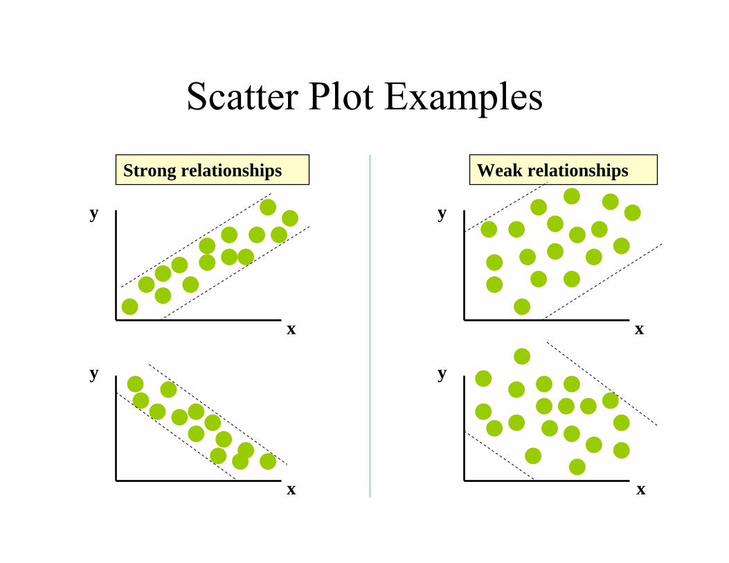
Scatter Plot Examples

y

x

y

x

y

y

x

x

Strong relationships Weak relationships

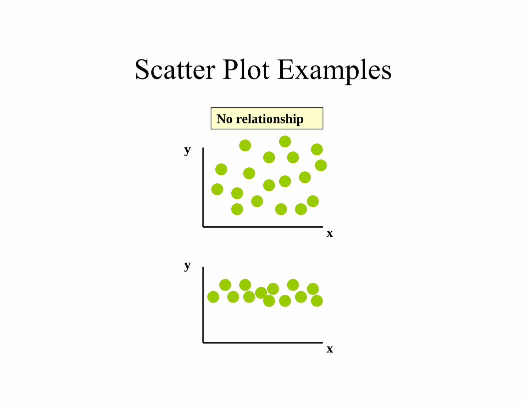
Scatter Plot Examples

y

x

y

x

No relationship

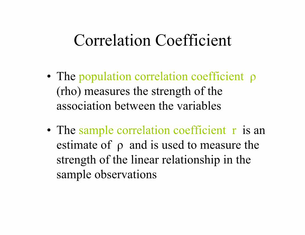
Correlation Coefficient

• The population correlation coefficient ρ(rho) measures the strength of the association between the variables

• The sample correlation coefficient r is an estimate of ρ and is used to measure the strength of the linear relationship in the sample observations

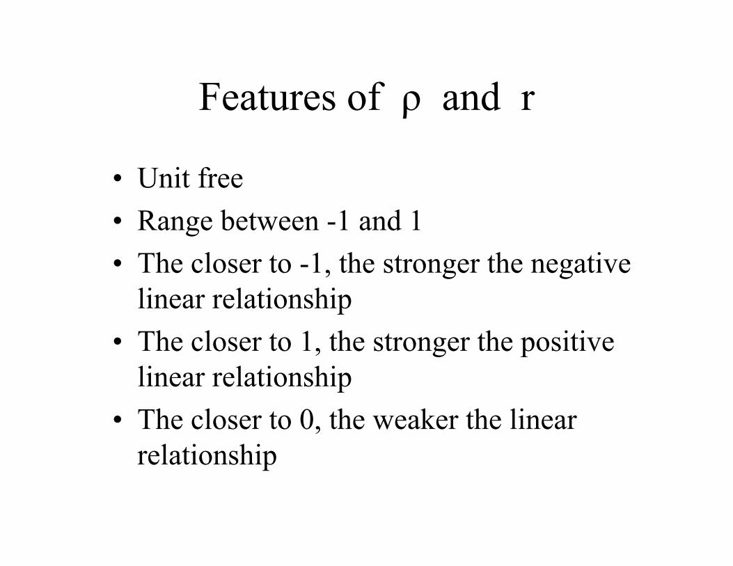
Features of ρ and r

• Unit free• Range between -1 and 1• The closer to -1, the stronger the negative

linear relationship• The closer to 1, the stronger the positive

linear relationship• The closer to 0, the weaker the linear

relationship

r = +.3 r = +1

Examples of Approximate r Values

y

x

y

x

y

x

y

x

y

x

r = -1 r = -.6 r = 0

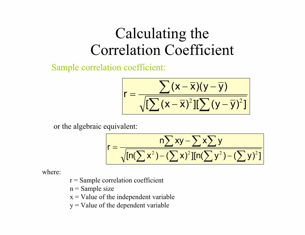
Calculating the Correlation Coefficient

∑∑∑

−−

−−=

])yy(][)xx([

)yy)(xx(r

22

where:r = Sample correlation coefficientn = Sample sizex = Value of the independent variabley = Value of the dependent variable

∑ ∑ ∑ ∑∑ ∑ ∑

−−

−=

])y()y(n][)x()x(n[

yxxynr

2222

Sample correlation coefficient:

or the algebraic equivalent:

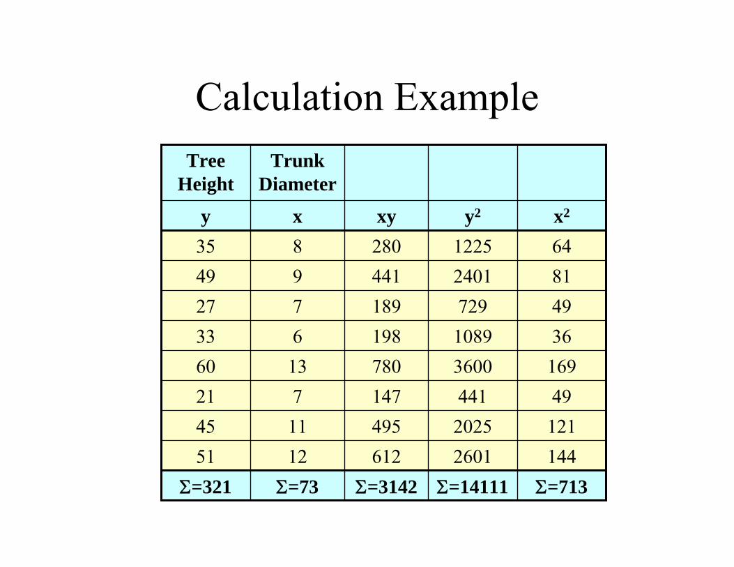
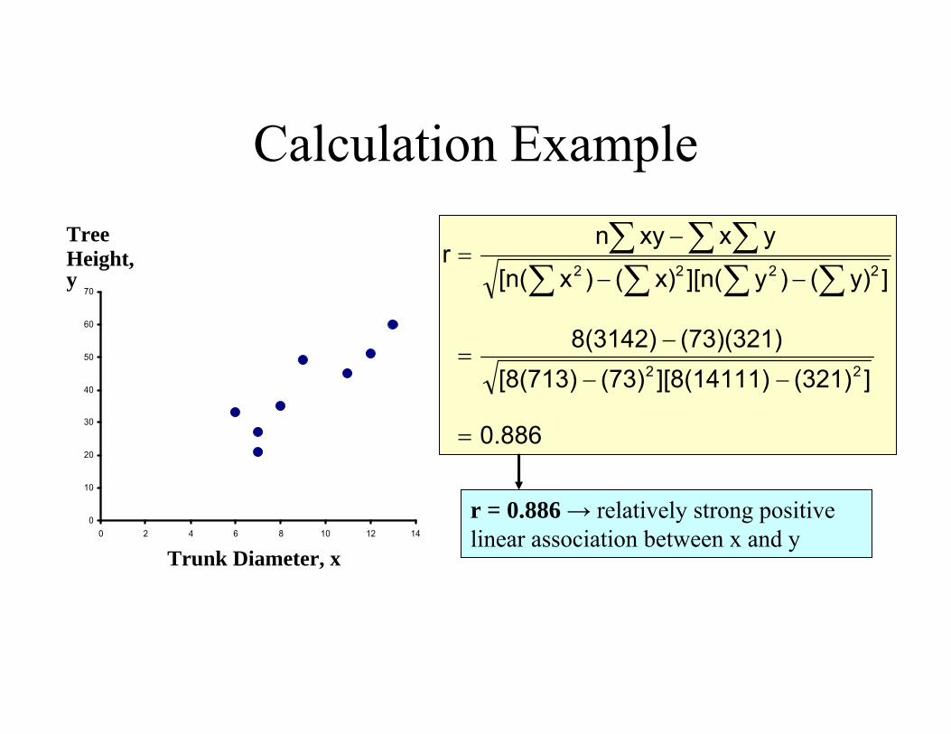
Calculation ExampleTrunk

DiameterTree

Height

Σ=713Σ=14111Σ=3142Σ=73Σ=321144260161212511212025495114549441147721

1693600780136036108919863349729189727812401441949641225280835x2y2xyxy

0

10

20

30

40

50

60

70

0 2 4 6 8 10 12 14

0.886

](321)][8(14111)(73)[8(713)(73)(321)8(3142)

]y)()y][n(x)()x[n(

yxxynr

22

2222

=

−−

−=

−−

−=

∑ ∑ ∑ ∑∑ ∑ ∑

Trunk Diameter, x

TreeHeight, y

Calculation Example

r = 0.886 → relatively strong positive linear association between x and y

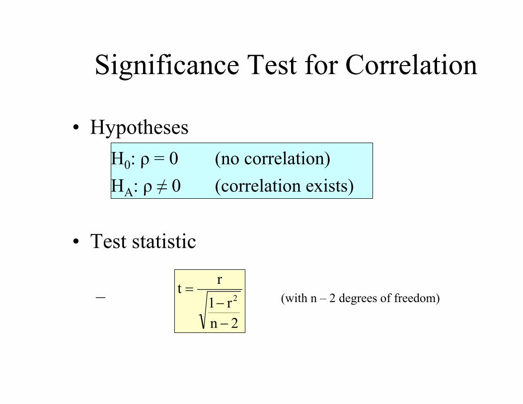
Significance Test for Correlation

• Hypotheses H0: ρ = 0 (no correlation) HA: ρ ≠ 0 (correlation exists)

• Test statistic

– (with n – 2 degrees of freedom)

2nr1

rt2

−−

=

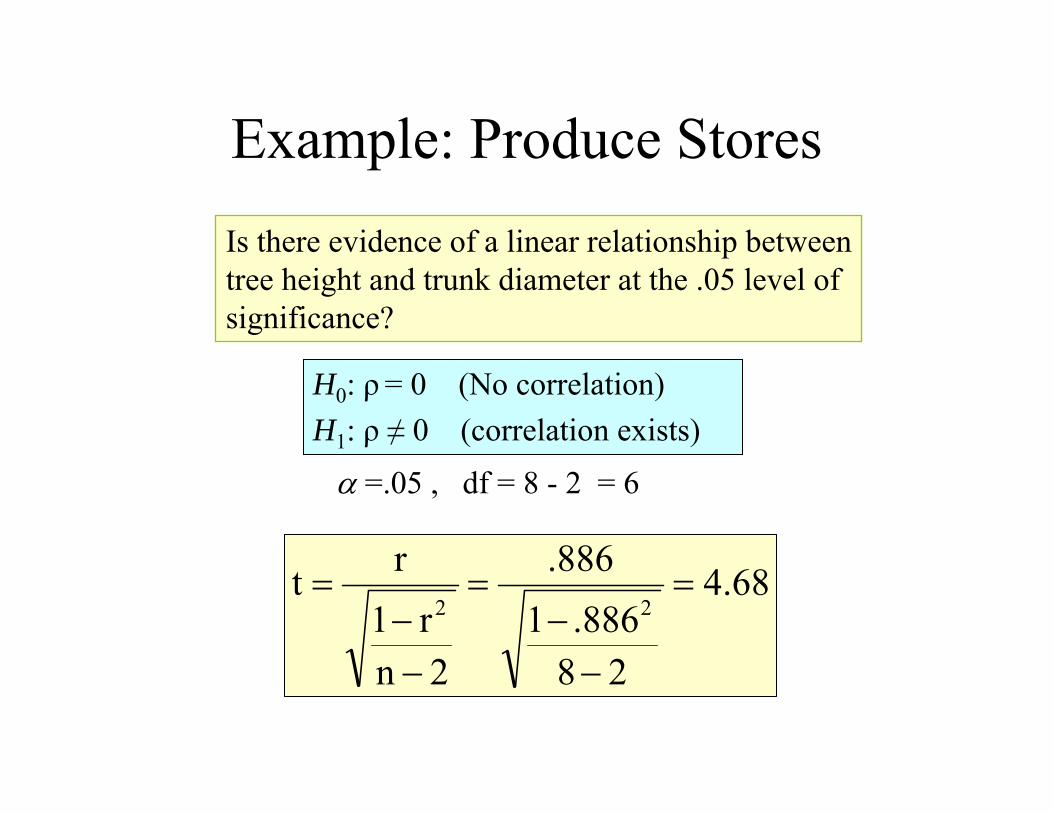
Example: Produce StoresIs there evidence of a linear relationship between tree height and trunk diameter at the .05 level of significance?

H0: ρ= 0 (No correlation)H1: ρ ≠ 0 (correlation exists)

α =.05 , df = 8 - 2 = 6

4.68

28.8861

.886

2nr1

rt22=

−−

=

−−

=

4.68

28.8861

.886

2nr1

rt22=

−−

=

−−

=

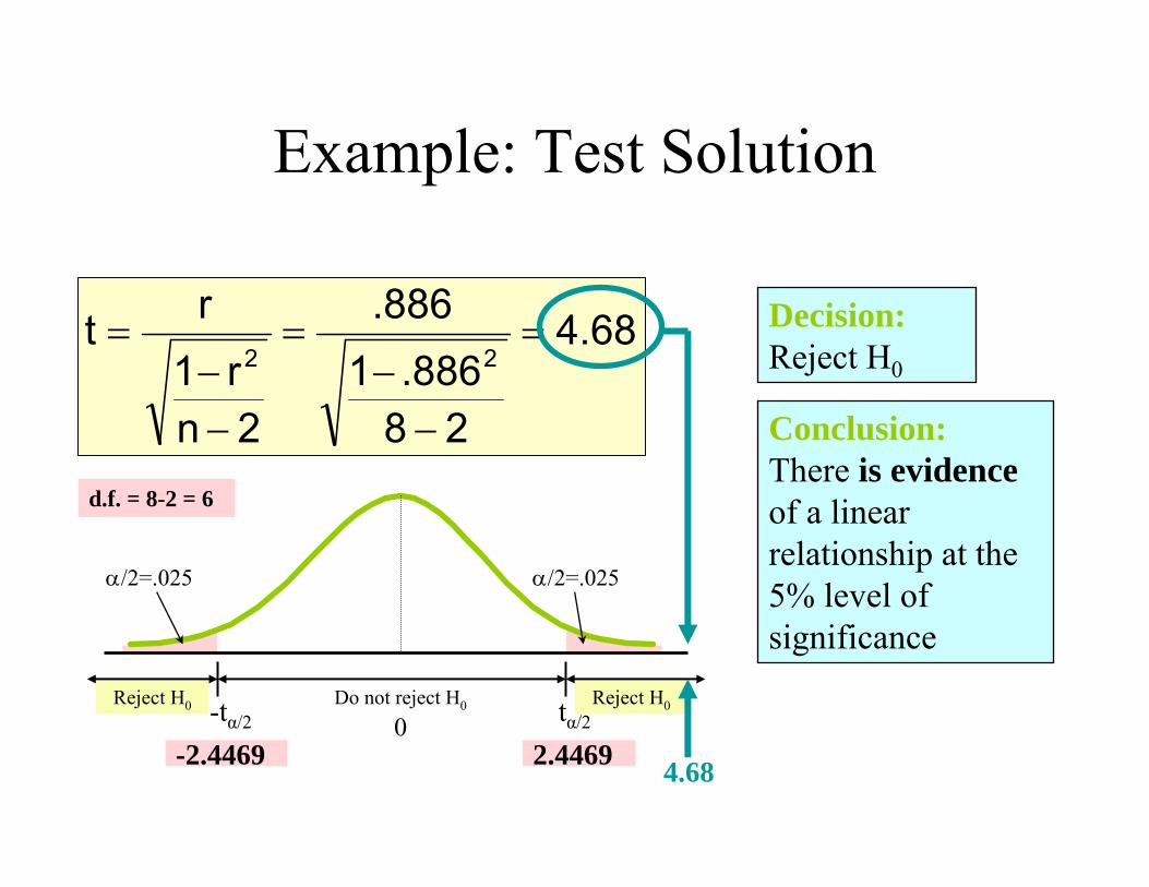
Example: Test Solution

Conclusion:There is evidenceof a linear relationship at the 5% level of significance

Decision:Reject H0

Reject H0Reject H0

α/2=.025

-tα/2Do not reject H0

0 tα/2

α/2=.025

-2.4469 2.4469 4.68

d.f. = 8-2 = 6

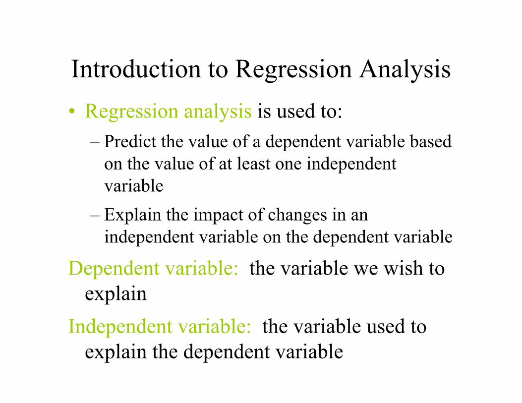
Introduction to Regression Analysis• Regression analysis is used to:

– Predict the value of a dependent variable based on the value of at least one independent variable

– Explain the impact of changes in an independent variable on the dependent variable

Dependent variable: the variable we wish to explain

Independent variable: the variable used to explain the dependent variable

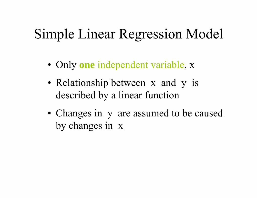
Simple Linear Regression Model

• Only one independent variable, x

• Relationship between x and y is described by a linear function

• Changes in y are assumed to be caused by changes in x

Types of Regression ModelsPositive Linear Relationship

Negative Linear Relationship

Relationship NOT Linear

No Relationship

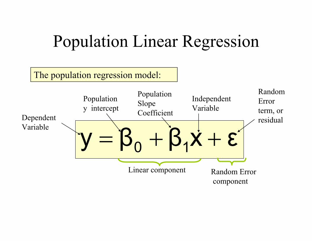
εxββy 10 ++=Linear component

Population Linear Regression

The population regression model:

Population y intercept

Population SlopeCoefficient

Random Error term, or residualDependent

Variable

Independent Variable

Random Errorcomponent

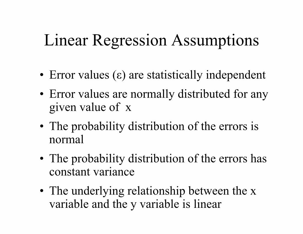
Linear Regression Assumptions

• Error values (ε) are statistically independent• Error values are normally distributed for any

given value of x• The probability distribution of the errors is

normal• The probability distribution of the errors has

constant variance• The underlying relationship between the x

variable and the y variable is linear

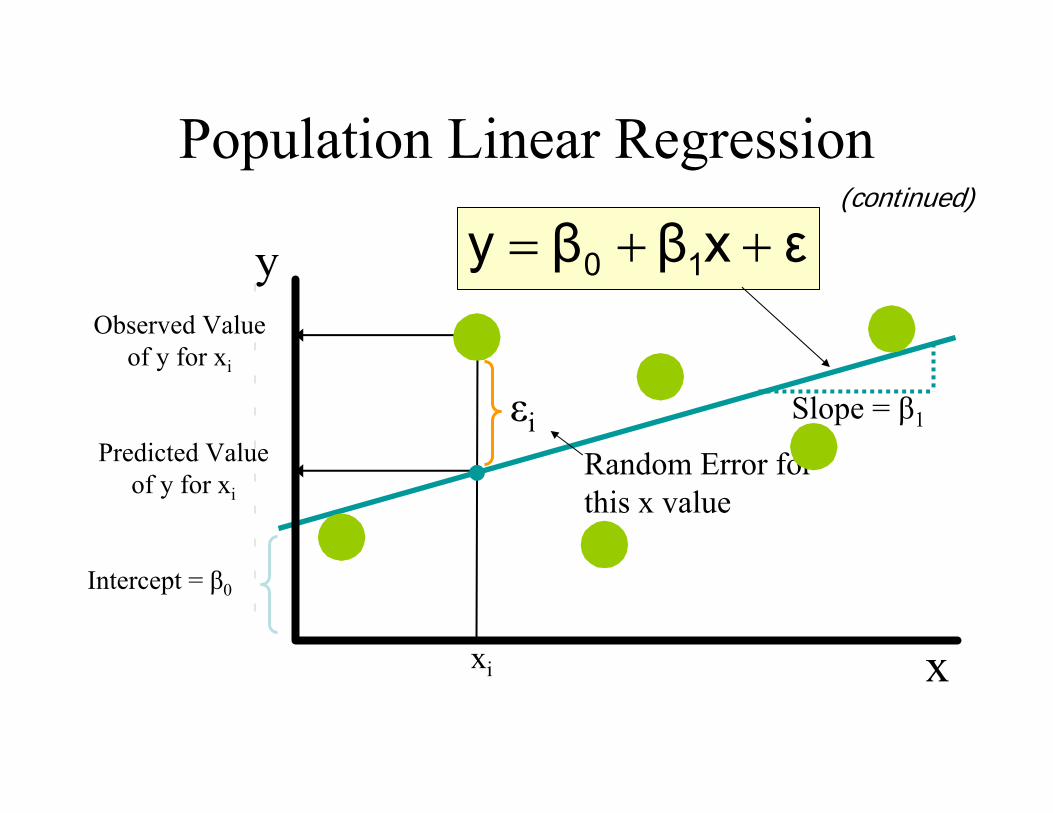
Population Linear Regression(continued)

Random Error for this x value

y

x

Observed Value of y for xi

Predicted Value of y for xi

εxββy 10 ++=

xi

Slope = β1

Intercept = β0

εi

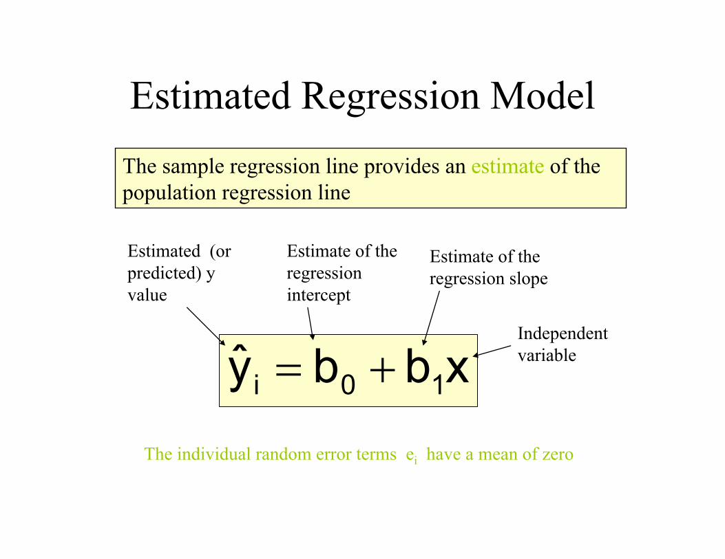
xbby 10i +=

The sample regression line provides an estimate of the population regression line

Estimated Regression Model

Estimate of the regression intercept

Estimate of the regression slope

Estimated (or predicted) y value

Independent variable

The individual random error terms ei have a mean of zero

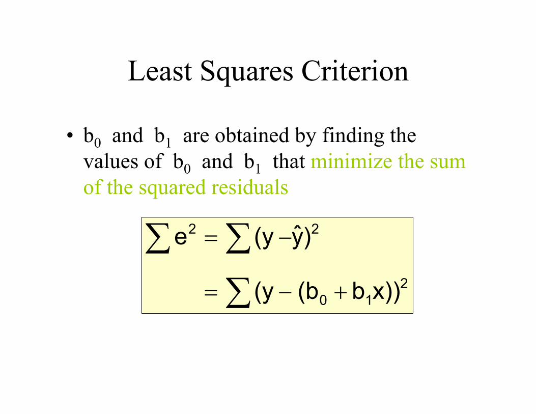
Least Squares Criterion

• b0 and b1 are obtained by finding the values of b0 and b1 that minimize the sum of the squared residuals

210

22

x))b(b(y

)y(ye

+−=

−=

∑∑∑

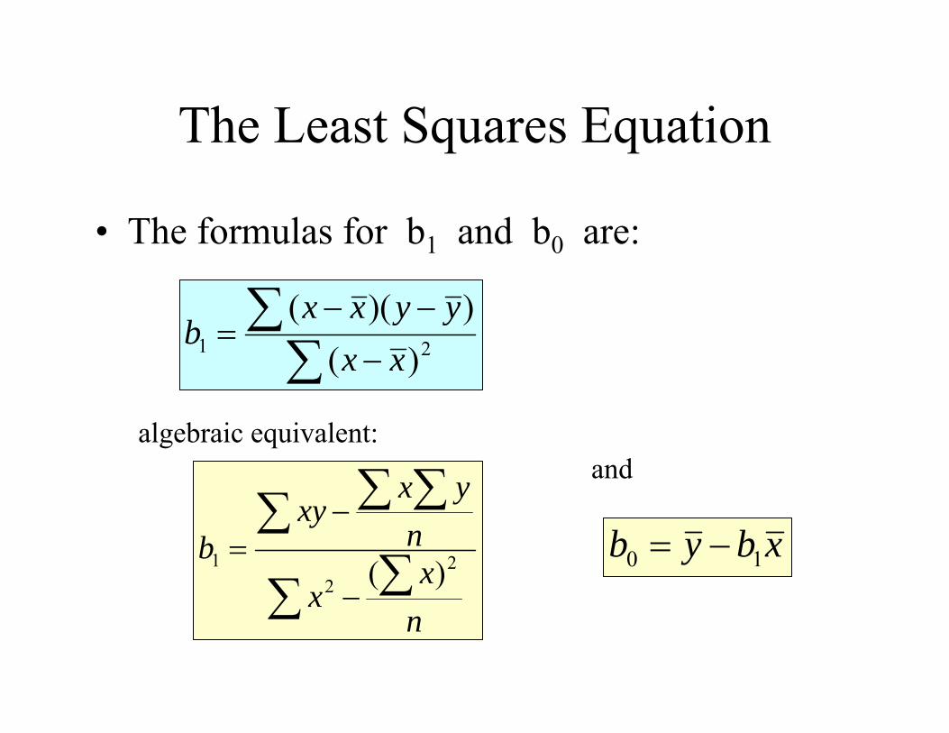
The Least Squares Equation

• The formulas for b1 and b0 are:

algebraic equivalent:

∑ ∑∑ ∑ ∑

−

−=

nx

x

nyx

xyb 2

21 )(

∑∑

−−−

= 21 )())((

xxyyxx

b

xbyb 10 −=

and

• b0 is the estimated average value of y when the value of x is zero

• b1 is the estimated change in the average value of y as a result of a one-unit change in x

Interpretation of the Slope and the Intercept

Finding the Least Squares Equation

• The coefficients b0 and b1 will usually be found using computer software

• Other regression measures will also be computed as part of computer-based regression analysis

Simple Linear Regression Example

• A real estate agent wishes to examine the relationship between the selling price of a home and its size (measured in square feet)

• A random sample of 10 houses is selected– Dependent variable (y) = house price in

$1000s– Independent variable (x) = square feet

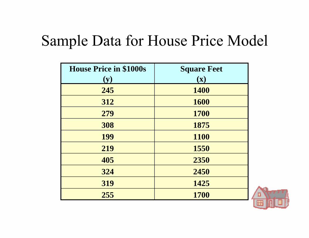
Sample Data for House Price Model

1700255142531924503242350405155021911001991875308170027916003121400245

Square Feet (x)

House Price in $1000s(y)

050

100150200250300350400450

0 500 1000 1500 2000 2500 3000

Square Feet

Hou

se P

rice

($10

00s)

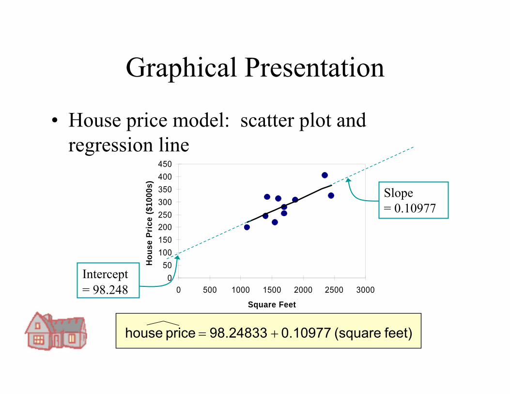
Graphical Presentation

• House price model: scatter plot and regression line

feet) (square 0.10977 98.24833 price house +=

Slope = 0.10977

Intercept = 98.248

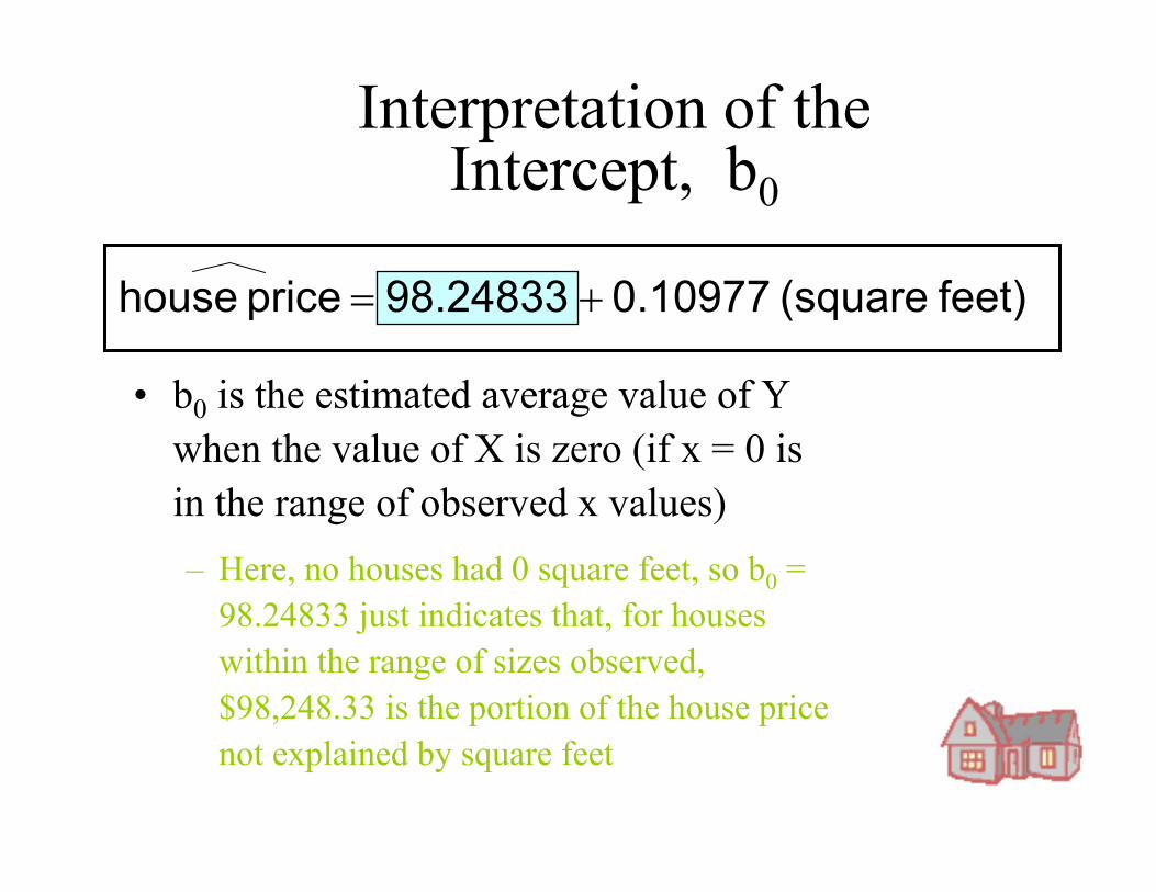
Interpretation of the Intercept, b0

• b0 is the estimated average value of Y when the value of X is zero (if x = 0 is in the range of observed x values)– Here, no houses had 0 square feet, so b0 =

98.24833 just indicates that, for houses within the range of sizes observed, $98,248.33 is the portion of the house price not explained by square feet

feet) (square 0.10977 98.24833 price house +=

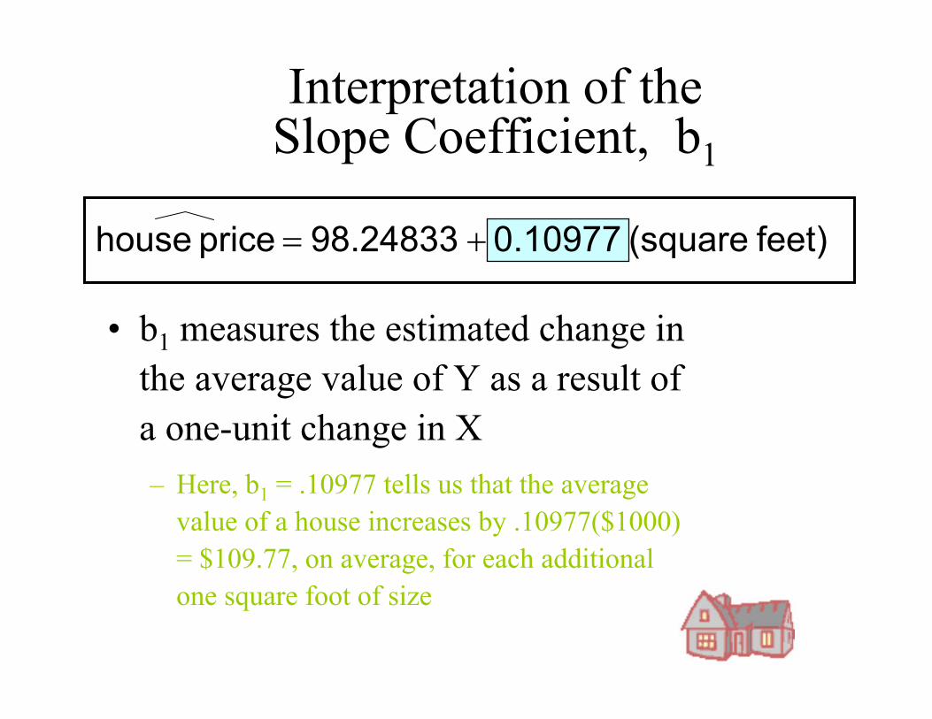
Interpretation of the Slope Coefficient, b1

• b1 measures the estimated change in the average value of Y as a result of a one-unit change in X– Here, b1 = .10977 tells us that the average

value of a house increases by .10977($1000) = $109.77, on average, for each additional one square foot of size

feet) (square 0.10977 98.24833 price house +=

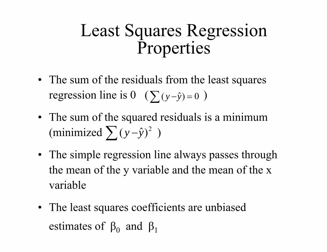
Least Squares Regression Properties

• The sum of the residuals from the least squares regression line is 0 ( )

• The sum of the squared residuals is a minimum (minimized )

• The simple regression line always passes through the mean of the y variable and the mean of the x variable

• The least squares coefficients are unbiased estimates of β0 and β1

0)ˆ( =−∑ yy

2)ˆ( yy∑ −

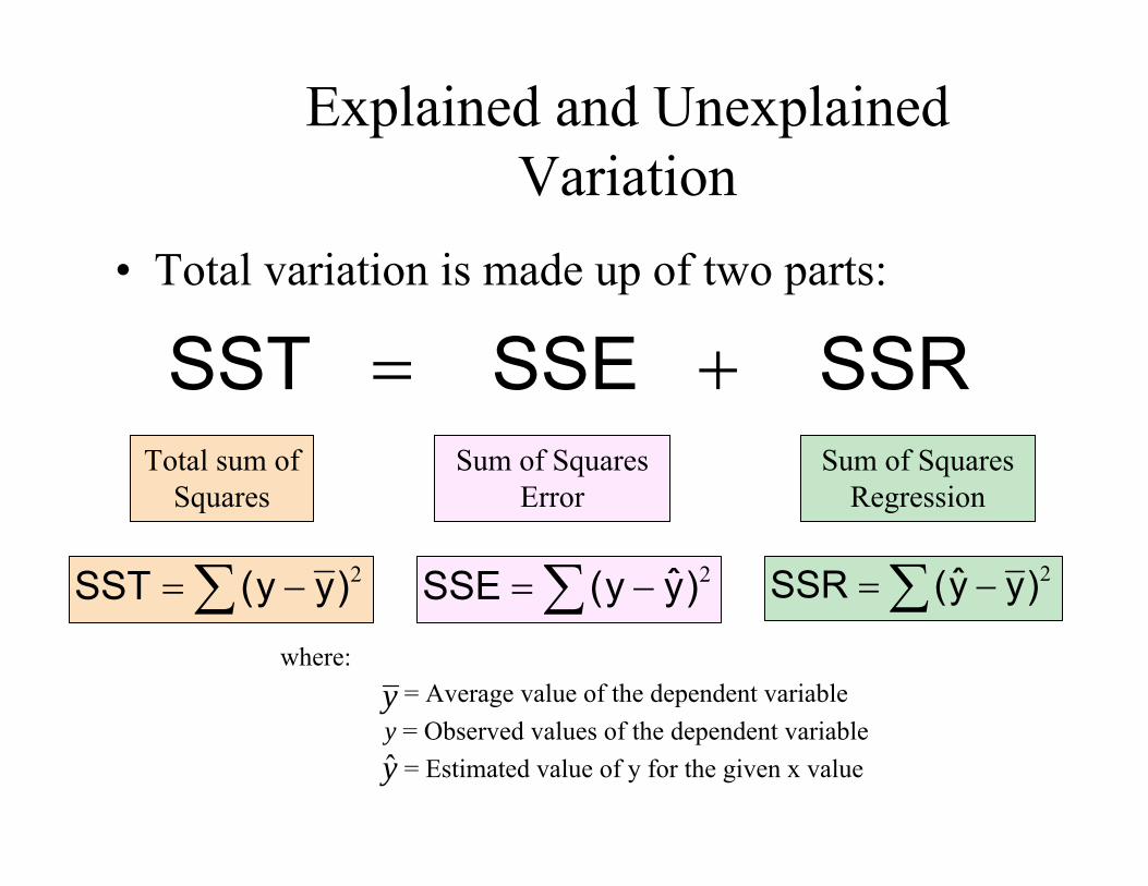
Explained and Unexplained Variation

• Total variation is made up of two parts:

SSR SSE SST +=Total sum of

SquaresSum of Squares

RegressionSum of Squares

Error

∑ −= 2)yy(SST ∑ −= 2)yy(SSE ∑ −= 2)yy(SSR

where:= Average value of the dependent variable

y = Observed values of the dependent variable= Estimated value of y for the given x valuey

y

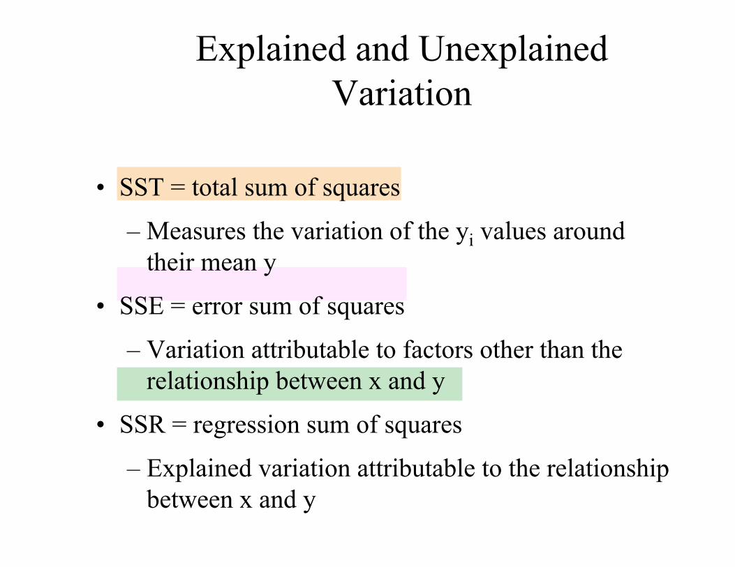
• SST = total sum of squares

– Measures the variation of the yi values around their mean y

• SSE = error sum of squares

– Variation attributable to factors other than the relationship between x and y

• SSR = regression sum of squares

– Explained variation attributable to the relationship between x and y

Explained and Unexplained Variation

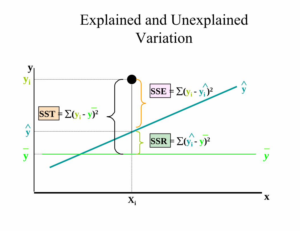
Xi

y

x

yi

SST = ∑(yi - y)2

SSE = ∑(yi - yi )2∧

SSR = ∑(yi - y)2∧

__

_

Explained and Unexplained Variation

y∧

y

y_y∧

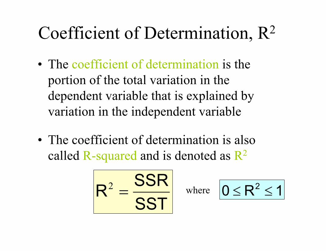
• The coefficient of determination is the portion of the total variation in the dependent variable that is explained by variation in the independent variable

• The coefficient of determination is also called R-squared and is denoted as R2

Coefficient of Determination, R2

SSTSSRR =2 1R0 2 ≤≤where

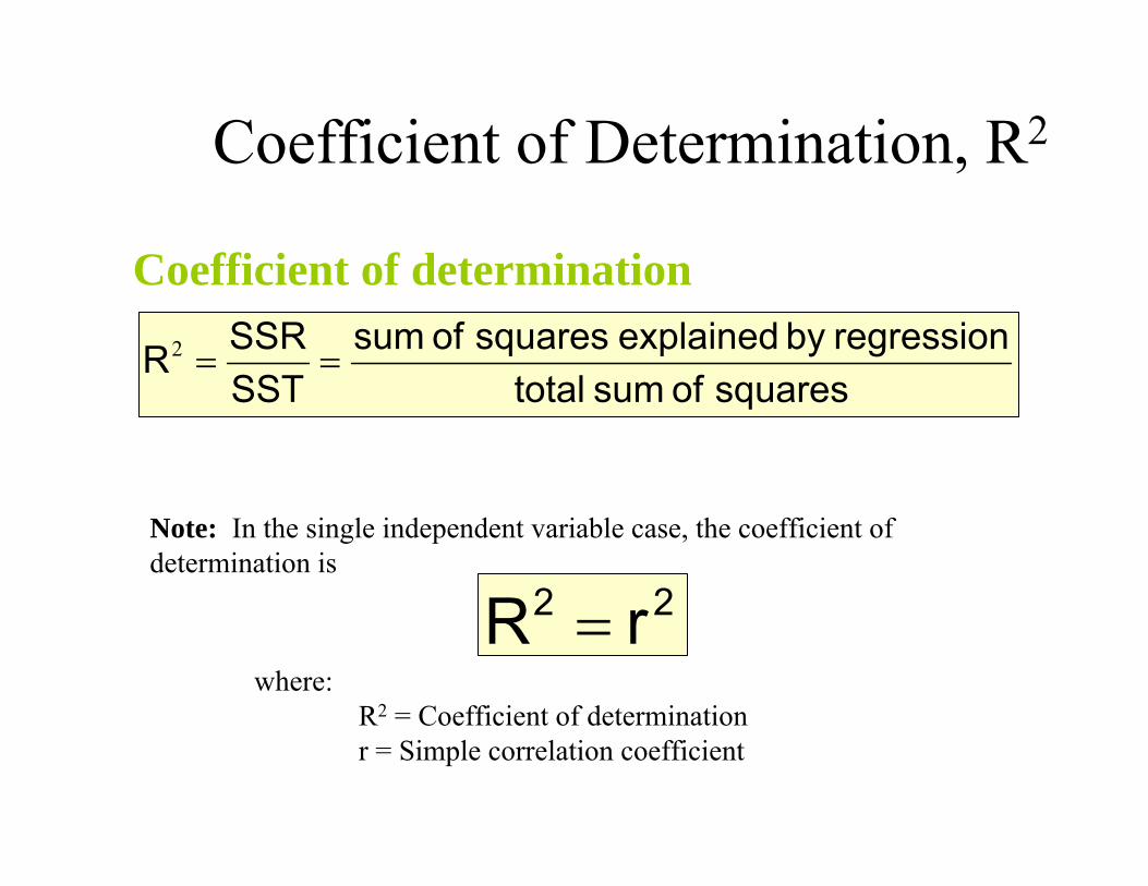
Coefficient of determination

Coefficient of Determination, R2

squares of sum totalregressionby explained squares of sum

SSTSSRR ==2

Note: In the single independent variable case, the coefficient of determination is

where:R2 = Coefficient of determinationr = Simple correlation coefficient

22 rR =

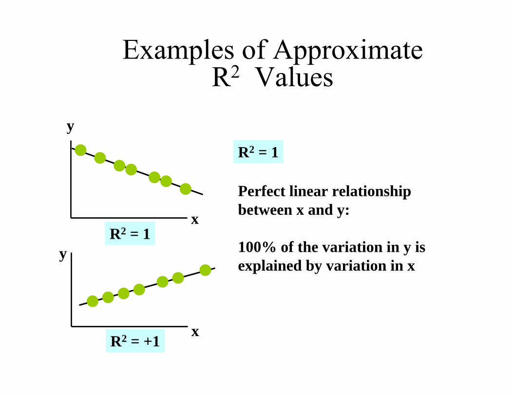
R2 = +1

Examples of Approximate R2 Values

y

x

y

x

R2 = 1

R2 = 1

Perfect linear relationship between x and y:

100% of the variation in y is explained by variation in x

Examples of Approximate R2 Values

y

x

y

x

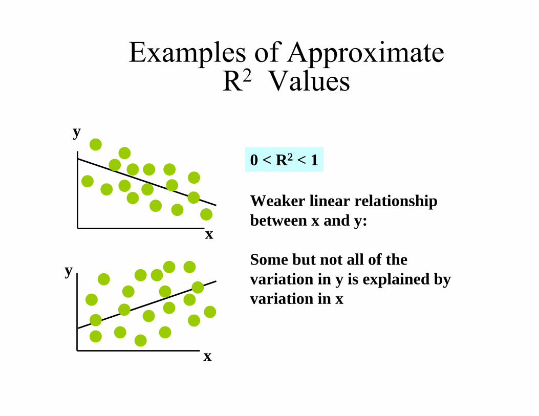
0 < R2 < 1

Weaker linear relationship between x and y:

Some but not all of the variation in y is explained by variation in x

Examples of Approximate R2 Values

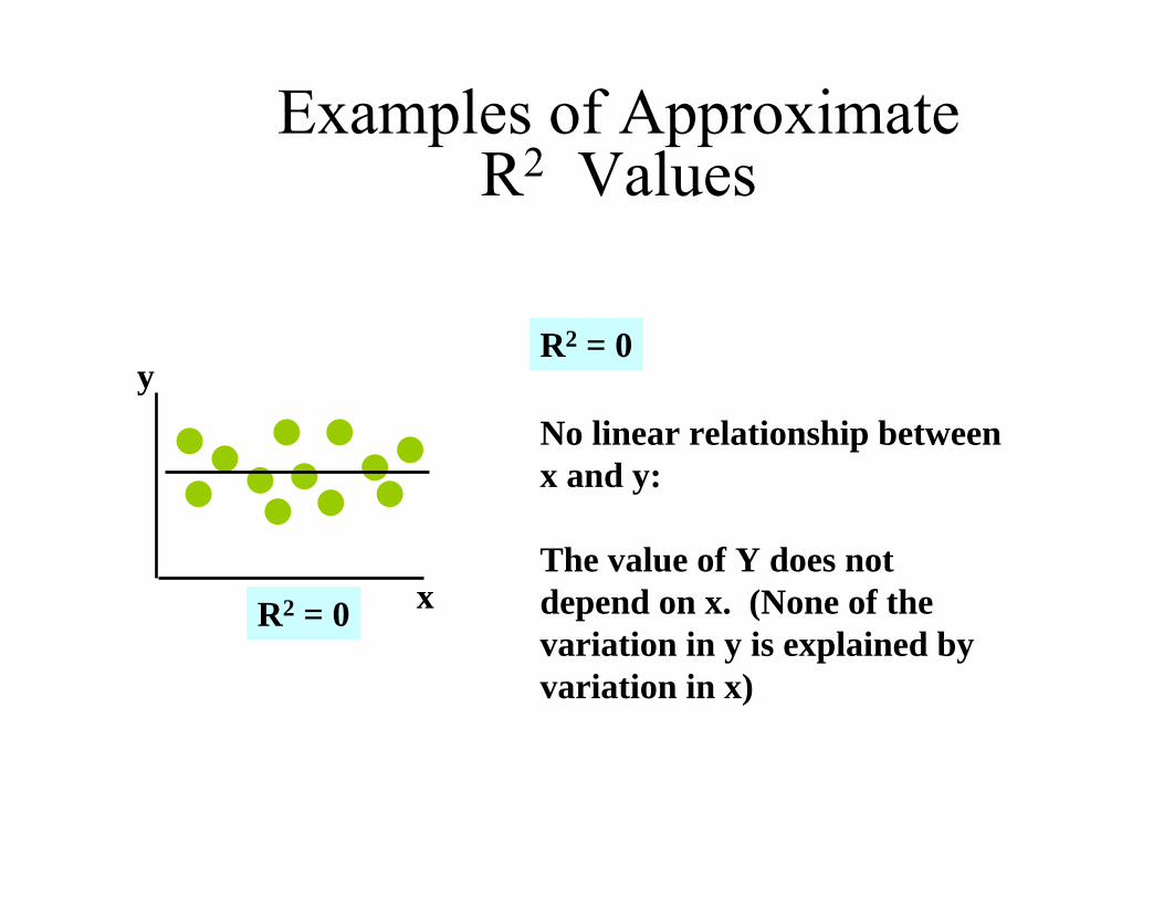
R2 = 0

No linear relationship between x and y:

The value of Y does not depend on x. (None of the variation in y is explained by variation in x)

y

xR2 = 0

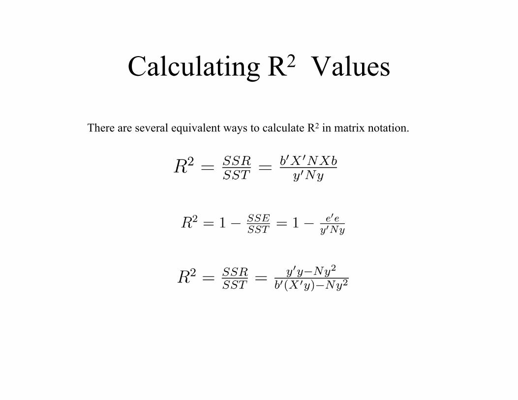
Calculating R2 Values

There are several equivalent ways to calculate R2 in matrix notation.

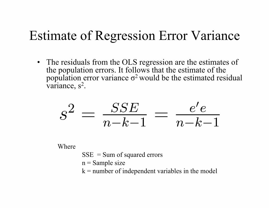
Estimate of Regression Error Variance

• The residuals from the OLS regression are the estimates of the population errors. It follows that the estimate of the population error variance σ2 would be the estimated residual variance, s2.

WhereSSE = Sum of squared errorsn = Sample sizek = number of independent variables in the model

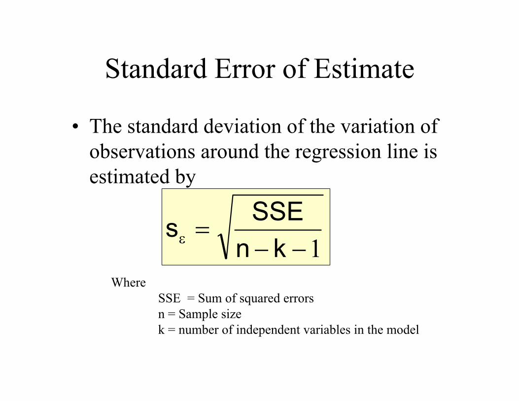
Standard Error of Estimate

• The standard deviation of the variation of observations around the regression line is estimated by

1−−=ε kn

SSEs

WhereSSE = Sum of squared errorsn = Sample sizek = number of independent variables in the model

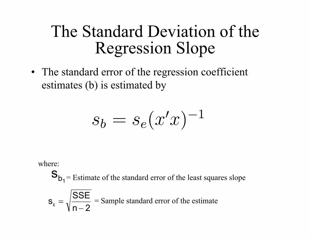
The Standard Deviation of the Regression Slope

• The standard error of the regression coefficient estimates (b) is estimated by

where:

= Estimate of the standard error of the least squares slope

= Sample standard error of the estimate

1bs

2nSSEsε −

=

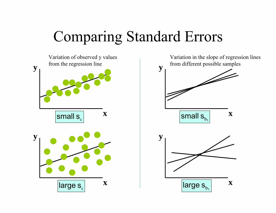
Comparing Standard Errors

y

y y

x

x

x

y

x

1bs small

1bs large

εs small

εs large

Variation of observed y values from the regression line

Variation in the slope of regression lines from different possible samples

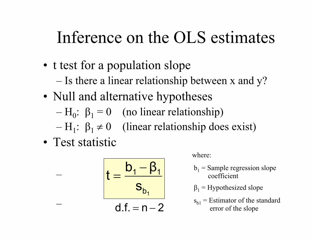
Inference on the OLS estimates• t test for a population slope

– Is there a linear relationship between x and y?• Null and alternative hypotheses

– H0: β1 = 0 (no linear relationship)– H1: β1 ≠ 0 (linear relationship does exist)

• Test statistic

–

–1b

11

sβbt −

=

2nd.f. −=

where:

b1 = Sample regression slopecoefficient

β1 = Hypothesized slope

sb1 = Estimator of the standarderror of the slope

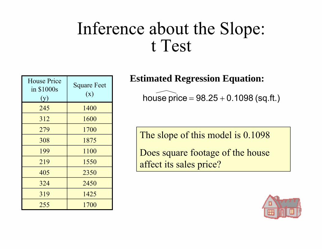
1700255142531924503242350405155021911001991875308170027916003121400245

Square Feet (x)

House Price in $1000s

(y) (sq.ft.) 0.1098 98.25 price house +=

Estimated Regression Equation:

The slope of this model is 0.1098

Does square footage of the house affect its sales price?

Inference about the Slope: t Test

Inferences about the Slope: t Test Example

H0: β1 = 0HA: β1 ≠ 0

Test Statistic: t = 3.329

There is sufficient evidence that square footage affects house price

From Excel output:

Reject H0

0.010393.329380.032970.10977Square Feet0.128921.6929658.0334898.24833InterceptP-valuet StatStandard ErrorCoefficients

1bs tb1

Decision:

Conclusion:

Reject H0Reject H0

α/2=.025

-tα/2Do not reject H0

0 tα/2

α/2=.025

-2.3060 2.3060 3.329

d.f. = 10-2 = 8

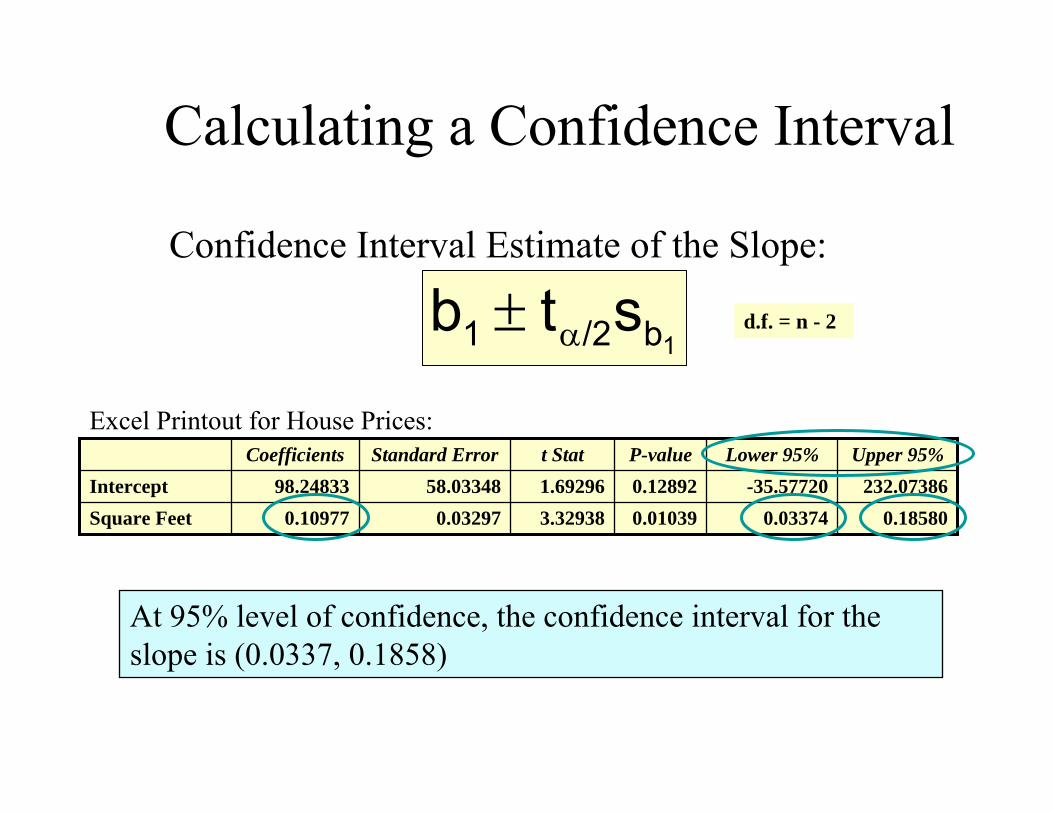
Calculating a Confidence Interval

Confidence Interval Estimate of the Slope:

Excel Printout for House Prices:

At 95% level of confidence, the confidence interval for the slope is (0.0337, 0.1858)

1b/21 stb α±

0.185800.033740.010393.329380.032970.10977Square Feet232.07386-35.577200.128921.6929658.0334898.24833Intercept

Upper 95%Lower 95%P-valuet StatStandard ErrorCoefficients

d.f. = n - 2

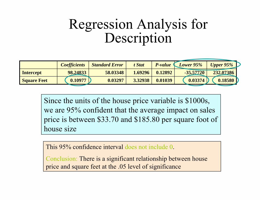
Regression Analysis for Description

Since the units of the house price variable is $1000s, we are 95% confident that the average impact on sales price is between $33.70 and $185.80 per square foot of house size

0.185800.033740.010393.329380.032970.10977Square Feet232.07386-35.577200.128921.6929658.0334898.24833Intercept

Upper 95%Lower 95%P-valuet StatStandard ErrorCoefficients

This 95% confidence interval does not include 0.

Conclusion: There is a significant relationship between house price and square feet at the .05 level of significance

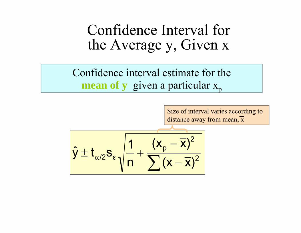
Confidence Interval for the Average y, Given x

Confidence interval estimate for the mean of y given a particular xp

Size of interval varies according to distance away from mean, x

∑ −−

+± α 2

2p

ε/2 )x(x)x(x

n1sty

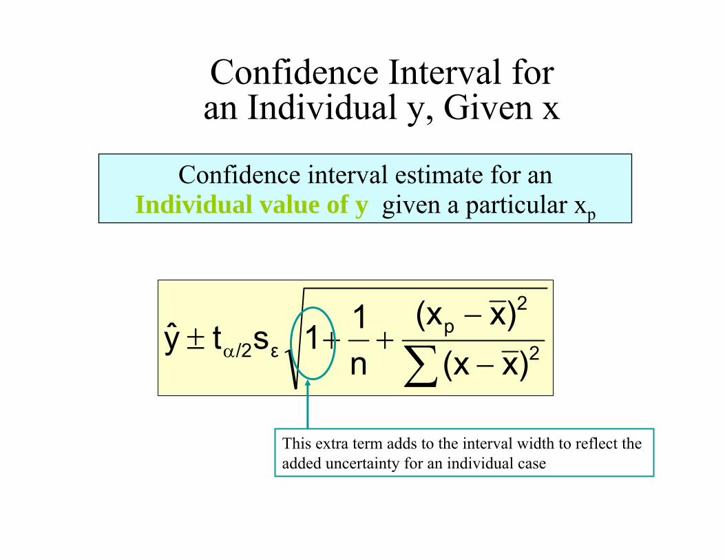
Confidence Interval for an Individual y, Given x

Confidence interval estimate for an Individual value of y given a particular xp

∑ −−

++± α 2

2p

ε/2 )x(x)x(x

n11sty

This extra term adds to the interval width to reflect the added uncertainty for an individual case

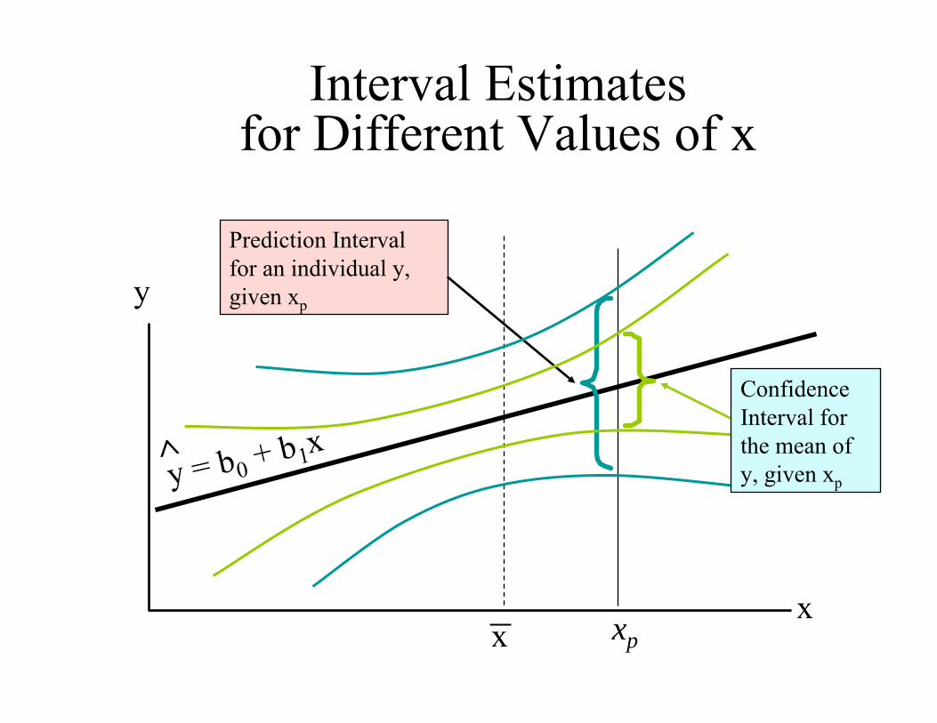
Interval Estimates for Different Values of x

y

x

Prediction Interval for an individual y, given xp

xp

y = b0 + b1x∧

x

Confidence Interval for the mean of y, given xp

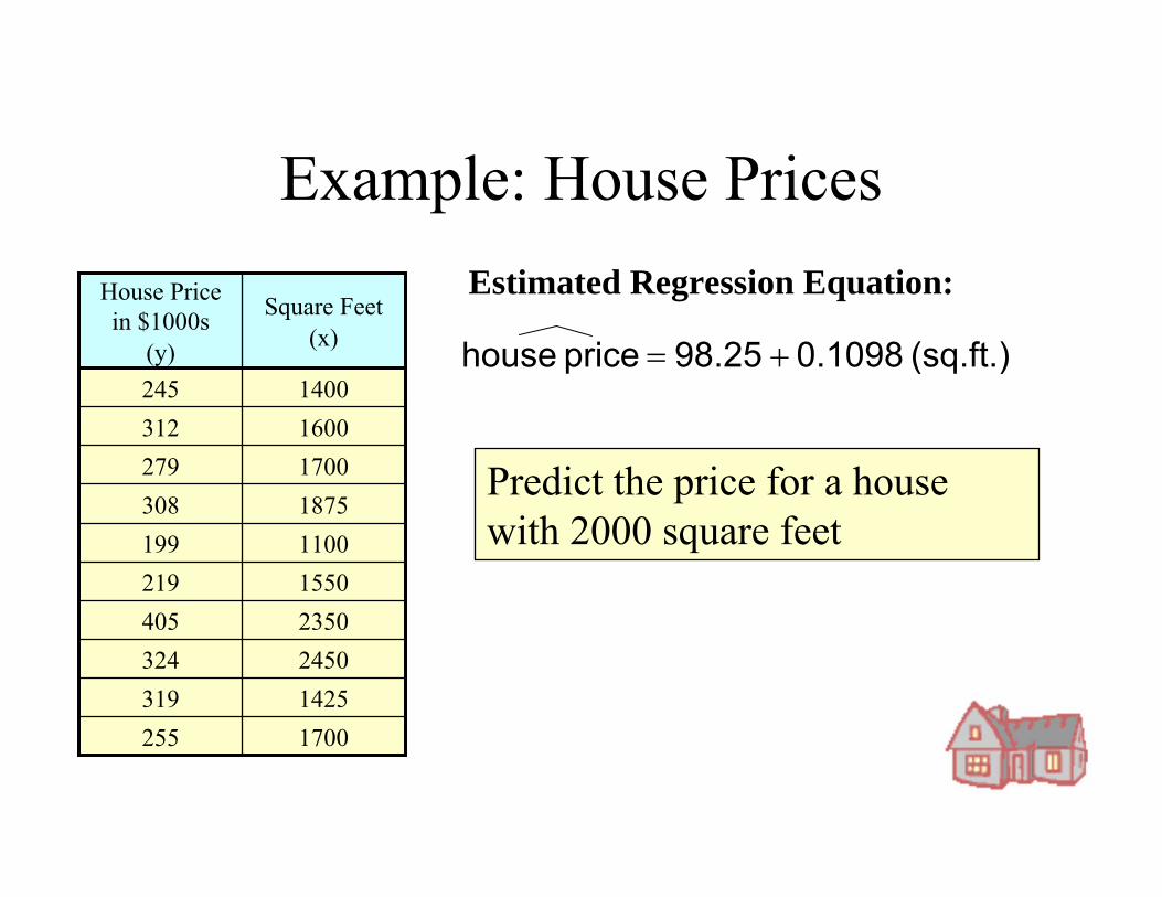
1700255142531924503242350405155021911001991875308170027916003121400245

Square Feet (x)

House Price in $1000s

(y) (sq.ft.) 0.1098 98.25 price house +=

Estimated Regression Equation:

Example: House Prices

Predict the price for a house with 2000 square feet

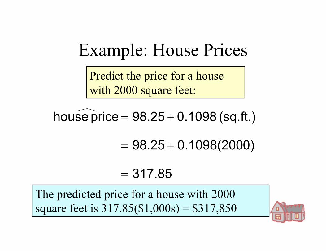
317.85

0)0.1098(200 98.25

(sq.ft.) 0.1098 98.25 price house

=

+=

+=

Example: House PricesPredict the price for a house with 2000 square feet:

The predicted price for a house with 2000 square feet is 317.85($1,000s) = $317,850

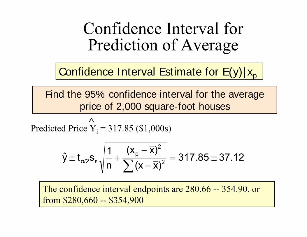
Confidence Interval for Prediction of Average

Find the 95% confidence interval for the average price of 2,000 square-foot houses

Predicted Price Yi = 317.85 ($1,000s)∧

Confidence Interval Estimate for E(y)|xp

37.12317.85)x(x

)x(xn1sty 2

2p

εα/2 ±=−−

+±∑

The confidence interval endpoints are 280.66 -- 354.90, or from $280,660 -- $354,900

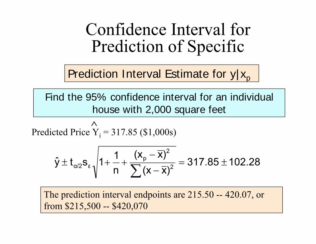
Confidence Interval for Prediction of Specific

Find the 95% confidence interval for an individual house with 2,000 square feet

Predicted Price Yi = 317.85 ($1,000s)∧

Prediction Interval Estimate for y|xp

102.28317.85)x(x

)x(xn11sty 2

2p

εα/2 ±=−−

++±∑

The prediction interval endpoints are 215.50 -- 420.07, or from $215,500 -- $420,070