introducing linear regression: an example using · pdf filejournal of economics and finance...

JOURNAL OF ECONOMICS AND FINANCE EDUCATION • Volume 11 • Number 2 • Winter 2012

113

Introducing Linear Regression: An Example Using

Basketball Statistics

Tom Arnold and Jonathan Godbey

1

ABSTRACT

The intuition behind linear regression can be difficult for students

to grasp particularly without a readily accessible context. This

paper uses basketball statistics to demonstrate the purpose of linear

regression and to explain how to interpret its results. In particular,

the student will quickly grasp the meaning of explanatory

variables, r-squared, and the statistical significance of estimates of

regression coefficients. Even if the student is not a sports fan the

examples are easily understood and familiar. The student can

easily replicate the procedures in this paper to reinforce learning.

Introduction

When calculators were introduced into the classroom, a number of tedious calculations could suddenly be

performed very quickly. However, students’ comprehension of mathematics did not actually improve and the

calculator in many ways masked deficiencies because a keystroke sequence could substitute for comprehension.

Regression analysis has some of the same characteristics because econometric software has improved to the

point that a regression is a simple one line command that results in copious amounts of output.

We believe the reason for the difficulty in understanding/interpreting regression results is not the product of

students being unable to perform the regression using matrix algebra, but the product of a lack of intuition that

belies the one line of code. In other words, it is equally important to understand why the regression is being

performed, what the regression process does to the data, and how to interpret the regression results.

By using the statistics from a basketball team, students become enabled to comprehend a model for

predicting the number of points a given player should be able to score based on certain factors. Regression is

then introduced as a means to calibrate and test the model.

The paper begins with a breakdown of what a regression “does” based on a very small set of data in which

hand calculators can perform all of the calculations. Next, the statistics from a basketball team are presented so

that a model can be generated to predict how many points should be scored in a game by an individual given a

set of factors. A regression is performed to calibrate and test the model. A second regression based on the

capital asset pricing model (Sharpe, 1964) is then performed on actual financial data. The paper concludes at

this point.

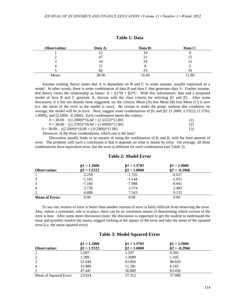
What Actually Happens in a Regression? Before introducing the basketball data, start with something even smaller. In Table 1, we have three

columns of data: A, B, and C with the averages of each column calculated by summing the data and dividing it

by the number of observations (5 in this case).

1 Tom Arnold, F. Carlyle Tiller Chair in Business, Robins School of Business, University of Richmond, 1 Gateway Road, Richmond, VA

23173; Jonathan M. Godbey, Clinical Assistant Professor, J. Mack College of Business, Georgia State University, 1209 RCB

Building, Atlanta, GA 30303. The authors would like to thank an anonymous referee, Jerry Stevens, David Greenberg, and

participants at the 2010 Financial Management Association Meetings for helpful comments.


114

Table 1: Data

Observation: Data A: Data B: Data C:

1 22 10 8

2 47 21 15

3 34 19 12

4 21 8 5

5 66 25 19

Mean: 38.00 16.60 11.80

Assume existing theory states that A is dependent on B and C in some manner, usually expressed as a

model. In other words, there is some combination of data B and data C that generates data A. Further assume,

that theory views the relationship as linear: A = β1*B + β2*C. With this information: data and a proposed

model of how B and C generate A, discuss with the class criteria for selecting β1 and β2. After some

discussion, if it has not already been suggested, try the criteria: Mean (A) less Mean (B) less Mean (C) is zero

(i.e. the mean of the error in the model is zero). Be certain to make the point: without this condition, on

average, the model will be in error. Next, suggest some combinations of β1 and β2: (1.2000, 1.5322), (1.5783,

1.0000), and (2.5000, -0.2966). Each combination meets the criteria:

0 = 38.00 – {(1.2000)*16.60 + (1.5322)*11.80} (1)

0 = 38.00 – {(1.5783)*16.60 + (1.0000)*11.80} (2)

0 = 38.00 – {(2.5000)*16.60 + (-0.2966)*11.80} (3)

However, of the three combinations, which one is the best?

Discussion usually leads to an answer of using the combination of β1 and β2 with the least amount of

error. The problem with such a conclusion is that it depends on what is meant by error. On average, all three

combinations have equivalent error, but the error is different for each combination (see Table 2).

Table 2: Model Error

Observation:

β1 = 1.2000

β2 = 1.5322

β1 = 1.5783

β2 = 1.0000

β1 = 2.5000

β2 = -0.2966

1 -2.258 -1.783 -0.627

2 -1.183 -1.144 -1.051

3 -7.186 -7.988 -9.941

4 3.739 3.374 2.483

5 6.888 7.543 9.135

Mean of Error: 0.00 0.00 0.00

To say one version of error is better than another version of error is fairly difficult from observing the error.

Also, unless a systematic rule is in place, there can be no consistent means of determining which version of the

error is best. After some more discussion (note: the discussion is important to get the student to understand the

issue and possibly resolve the issue), suggest looking at the square of the error and take the mean of the squared

error (i.e. the mean squared error).

Table 3: Model Squared Error

Observation:

β1 = 1.2000

β2 = 1.5322

β1 = 1.5783

β2 = 1.0000

β1 = 2.5000

β2 = -0.2966

1 5.097 3.197 0.393

2 1.399 1.3089 1.105

3 51.644 63.803 98.820

4 13.980 11.381 6.165

5 47.447 56.889 83.456

Mean of Squared Error: 23.914 27.312 37.988


115

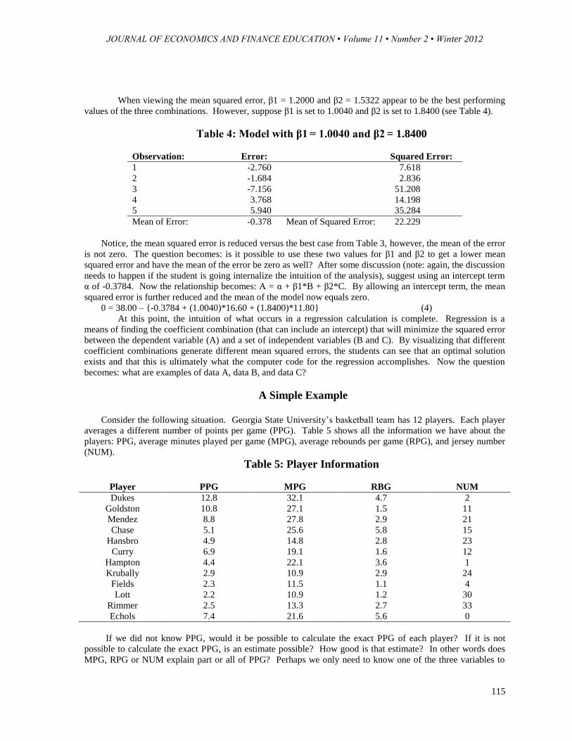
When viewing the mean squared error, β1 = 1.2000 and β2 = 1.5322 appear to be the best performing

values of the three combinations. However, suppose β1 is set to 1.0040 and β2 is set to 1.8400 (see Table 4).

Table 4: Model with β1 = 1.0040 and β2 = 1.8400

Observation: Error: Squared Error:

1 -2.760 7.618

2 -1.684 2.836

3 -7.156 51.208

4 3.768 14.198

5 5.940 35.284

Mean of Error: -0.378 Mean of Squared Error: 22.229

Notice, the mean squared error is reduced versus the best case from Table 3, however, the mean of the error

is not zero. The question becomes: is it possible to use these two values for β1 and β2 to get a lower mean

squared error and have the mean of the error be zero as well? After some discussion (note: again, the discussion

needs to happen if the student is going internalize the intuition of the analysis), suggest using an intercept term

α of -0.3784. Now the relationship becomes: A = α + β1*B + β2*C. By allowing an intercept term, the mean

squared error is further reduced and the mean of the model now equals zero.

0 = 38.00 – {-0.3784 + (1.0040)*16.60 + (1.8400)*11.80} (4)

At this point, the intuition of what occurs in a regression calculation is complete. Regression is a

means of finding the coefficient combination (that can include an intercept) that will minimize the squared error

between the dependent variable (A) and a set of independent variables (B and C). By visualizing that different

coefficient combinations generate different mean squared errors, the students can see that an optimal solution

exists and that this is ultimately what the computer code for the regression accomplishes. Now the question

becomes: what are examples of data A, data B, and data C?

A Simple Example

Consider the following situation. Georgia State University’s basketball team has 12 players. Each player

averages a different number of points per game (PPG). Table 5 shows all the information we have about the

players: PPG, average minutes played per game (MPG), average rebounds per game (RPG), and jersey number

(NUM).

Table 5: Player Information

Player PPG MPG RBG NUM

Dukes 12.8 32.1 4.7 2

Goldston 10.8 27.1 1.5 11

Mendez 8.8 27.8 2.9 21

Chase 5.1 25.6 5.8 15

Hansbro 4.9 14.8 2.8 23

Curry 6.9 19.1 1.6 12

Hampton 4.4 22.1 3.6 1

Krubally 2.9 10.9 2.9 24

Fields 2.3 11.5 1.1 4

Lott 2.2 10.9 1.2 30

Rimmer 2.5 13.3 2.7 33

Echols 7.4 21.6 5.6 0

If we did not know PPG, would it be possible to calculate the exact PPG of each player? If it is not

possible to calculate the exact PPG, is an estimate possible? How good is that estimate? In other words does

MPG, RPG or NUM explain part or all of PPG? Perhaps we only need to know one of the three variables to


116

estimate PPG. Maybe one is enough to get an approximate estimate but knowing one or both of the others will

give us a more precise estimate. Linear regression provides the means to answer these questions.

Note that we only have 12 players. It makes sense that using more observations would make us more

confident in our estimates. If we were truly trying to answer the question of what explains PPG we would want

data from many other teams. However, for purposes of trying to “see” what is happening with the numbers it is

better to keep the number of observations small.

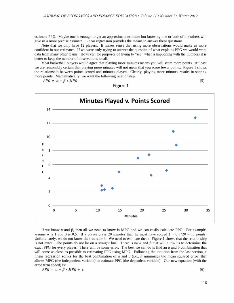
Most basketball players would agree that playing more minutes means you will score more points. At least

we are reasonably certain that playing more minutes will not mean that you score fewer points. Figure 1 shows

the relationship between points scored and minutes played. Clearly, playing more minutes results in scoring

more points. Mathematically, we want the following relationship.

(5)

Figure 1

If we know α and β, then all we need to know is MPG and we can easily calculate PPG. For example,

assume α is 1 and β is 0.5. If a player plays 20 minutes then he must have scored 1 + 0.5*20 = 11 points.

Unfortunately, we do not know the true α or β. We need to estimate them. Figure 1 shows that the relationship

is not exact. The points do not lie on a straight line. There is no α and β that will allow us to determine the

exact PPG for every player. There will be some error. The best we can do is find an α and β combination that

will come as close as possible to estimating PPG using MPG. Following the intuition from the last section, a

linear regression solves for the best combination of α and β (i.e., it minimizes the mean squared error) that

allows MPG (the independent variable) to estimate PPG (the dependent variable). Our new equation (with the

error term added) is:

(6)

0

2

4

6

8

10

12

14

0 5 10 15 20 25 30 35

P

o

i

n

t

s

Minutes

Minutes Played v. Points Scored


117

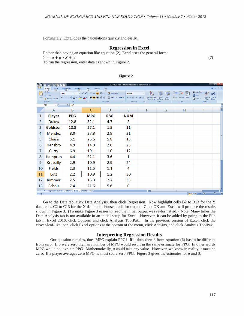
Fortunately, Excel does the calculations quickly and easily.

Regression in Excel Rather than having an equation like equation (2), Excel uses the general form:

. (7)

To run the regression, enter data as shown in Figure 2.

Figure 2

Go to the Data tab, click Data Analysis, then click Regression. Now highlight cells B2 to B13 for the Y

data, cells C2 to C13 for the X data, and choose a cell for output. Click OK and Excel will produce the results

shown in Figure 3. (To make Figure 3 easier to read the initial output was re-formatted.) Note: Many times the

Data Analysis tab is not available in an initial setup for Excel. However, it can be added by going to the File

tab in Excel 2010, click Options, and click Analysis ToolPak. In the previous version of Excel, click the

clover-leaf-like icon, click Excel options at the bottom of the menu, click Add-ins, and click Analysis ToolPak.

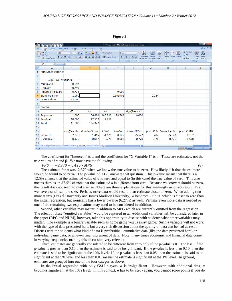
Interpreting Regression Results Our question remains, does MPG explain PPG? If it does then β from equation (6) has to be different

from zero. If β were zero then any number of MPG would result in the same estimate for PPG. In other words

MPG would not explain PPG. Mathematically, α could take any value. However, we know in reality it must be

zero. If a player averages zero MPG he must score zero PPG. Figure 3 gives the estimates for α and β.


118

Figure 3

The coefficient for “Intercept” is α and the coefficient for “X Variable 1” is β. These are estimates, not the

true values of α and β. We now have the following.

(8)

The estimate for α was -2.370 when we know the true value to be zero. How likely is it that the estimate

would be found to be zero? The p-value of 0.125 answers that question. This p-value means that there is a

12.5% chance that the estimated value of α is zero and equal to (in this case) the true value of zero. This also

means there is an 87.5% chance that the estimated α is different from zero. Because we know α should be zero,

this result does not seem to make sense. There are three explanations for this seemingly incorrect result. First,

we have a small sample size. Perhaps more data would result in an estimate closer to zero. When adding two

more teams (Drexel University and James Madison University), α becomes -0.9950 which is closer to zero than

the initial regression, but ironically has a lower p-value (6.27%) as well. Perhaps even more data is needed or

one of the remaining two explanations may need to be considered in addition.

Second, other variables may matter in addition to MPG which are currently omitted from the regression.

The effect of these “omitted variables” would be captured in α. Additional variables will be considered later in

the paper (RPG and NUM), however, take this opportunity to discuss with students what other variables may

matter. One example is a binary variable such as home game versus away game. Such a variable will not work

with the type of data presented here, but a very rich discussion about the quality of data can be had as result.

Discuss with the students what kind of data is preferable…cumulative data (like the data presented here) or

individual game data, or an even finer increment of data. Note: many times economic and financial data come

in varying frequencies making this discussion very relevant.

Third, estimates are generally considered to be different from zero only if the p-value is 0.10 or less. If the

p-value is greater than 0.10 then the estimate is said to be insignificant. If the p-value is less than 0.10, then the

estimate is said to be significant at the 10% level. If the p-value is less than 0.05, then the estimate is said to be

significant at the 5% level and less than 0.01 means the estimate is significant at the 1% level. In general,

estimates are grouped into one of the four categories above.

In the initial regression with only GSU players, α is insignificant. However, with additional data, α

becomes significant at the 10% level. In this context, α has to be zero (again, you cannot score points if you do


119

not play) and being estimated as different from zero while being insignificant is “statistically” the equivalent of

being zero. The initial regression demonstrates this case. However, with additional data, the estimate for α gets

closer to zero, but then becomes significant. Although an apparently “confounding result”, this is not an

uncommon situation and as discussed earlier leads to the desire for more data, more variables, or both to address

the confounding result.

It should be noted, that many times the true value of α is not known with any certainty within a particular

model and analyzing the estimated α is simply a matter of determining if the estimated α is different from zero.

In this case, α is known to be zero which allowed for a more in depth discussion of the regression model not

being fully accurate.

The estimate for β was 0.420. If the true value of β is different from zero then MPG is useful in explaining

PPG. Is 0.420 close to zero? Once again, the p-value of 0.000098 answers that question. (Note Figure 3 shows

the rounded result 0.000). This means that there is a 0.0098% chance that the true value of β is zero and our

estimate is different from zero as a result of chance. In other words, we are 99.9902% sure that the true β is not

zero. MPG matters. MPG is significant at the 1% level.

MPG matters, but does it explain all of PPG? Would knowing RPG (average rebounds per game) or NUM

(jersey number) help in the estimation of PPG? The r-square given in Figure 3 indicates the percentage of the

variation of PPG that is explained by MPG. The result of 0.795 means that 79.5% of the variation in PPG is

explained by MPG (Note: this is an upwardly biased estimate and more analysis presented later in this paper can

be used to address this issue). If the result had been 1.000 then MPG would explain 100% of the variation in

PPG. Because not all of the variation in PPG is explained by MPG, let us consider searching for more

explanatory variables.

Multivariate Regressions The significance of multiple variables can be checked simultaneously. Suppose we want to see if RPG and

NUM in addition to MPG are important in explaining PPG because we believe more variables are necessary to

produce a better estimation of PPG. We, then, run the following regression.

(9)

To run this regression, enter data as shown in Figure 2. Go to the Data tab, click Data Analysis, then click

Regression. Now highlight cells B2 to B13 for the Y data, cells C2 to E13 for the X data, and choose a cell for

output. Click OK and Excel will produce the results shown in Figure 4. (To make Figure 4 easier to read the

initial output was re-formatted.)


120

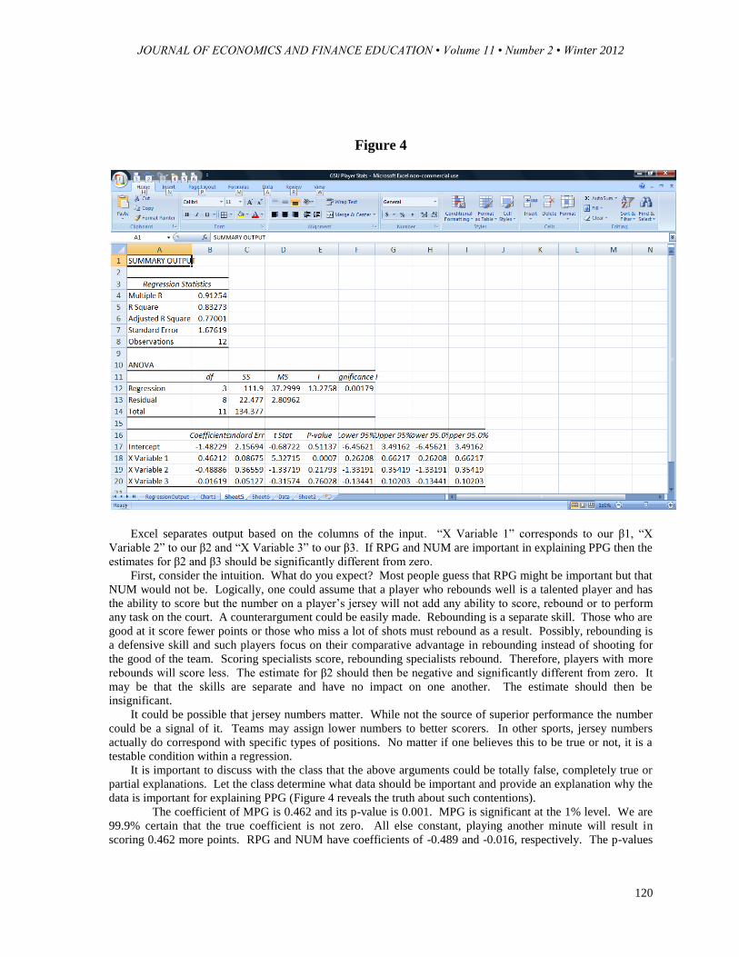
Figure 4

Excel separates output based on the columns of the input. “X Variable 1” corresponds to our β1, “X

Variable 2” to our β2 and “X Variable 3” to our β3. If RPG and NUM are important in explaining PPG then the

estimates for β2 and β3 should be significantly different from zero.

First, consider the intuition. What do you expect? Most people guess that RPG might be important but that

NUM would not be. Logically, one could assume that a player who rebounds well is a talented player and has

the ability to score but the number on a player’s jersey will not add any ability to score, rebound or to perform

any task on the court. A counterargument could be easily made. Rebounding is a separate skill. Those who are

good at it score fewer points or those who miss a lot of shots must rebound as a result. Possibly, rebounding is

a defensive skill and such players focus on their comparative advantage in rebounding instead of shooting for

the good of the team. Scoring specialists score, rebounding specialists rebound. Therefore, players with more

rebounds will score less. The estimate for β2 should then be negative and significantly different from zero. It

may be that the skills are separate and have no impact on one another. The estimate should then be

insignificant.

It could be possible that jersey numbers matter. While not the source of superior performance the number

could be a signal of it. Teams may assign lower numbers to better scorers. In other sports, jersey numbers

actually do correspond with specific types of positions. No matter if one believes this to be true or not, it is a

testable condition within a regression.

It is important to discuss with the class that the above arguments could be totally false, completely true or

partial explanations. Let the class determine what data should be important and provide an explanation why the

data is important for explaining PPG (Figure 4 reveals the truth about such contentions).

The coefficient of MPG is 0.462 and its p-value is 0.001. MPG is significant at the 1% level. We are

99.9% certain that the true coefficient is not zero. All else constant, playing another minute will result in

scoring 0.462 more points. RPG and NUM have coefficients of -0.489 and -0.016, respectively. The p-values


121

are 0.218 and 0.760. Neither one is significant at the 10% level and therefore both are considered insignificant.

In other words, they do not matter.

The intercept (α) is -1.482, which is closer to zero than when estimated in the initial regression with

only MPG as an independent variable. Unlike the initial regression, one cannot definitively state that α should

be zero because RPG and NUM have also been included.in the regression. However, RPG and NUM are

considered insignificant while MPG is still significant. Consequently, because RPG and NUM are insignificant,

it again makes sense for α to be zero. As stated before, α is closer to zero than it had been in the initial

regression, but what is more striking is how much more insignificant α has become: p-value = 0.511 versus a p-

value of 0.125 previously. Again, “statistically”, α is effectively estimated to be zero.

The r-square is 0.833 which is higher than the r-square of the regression containing only MPG. R-square

will never fall if additional explanatory variables are added. It may even rise if additional insignificant

explanatory variables are added. This result demonstrates a weakness of r-square. The addition RPG and NUM

which do not matter in the estimation of PPG should not cause r-square to rise. To address this issue the

measure “adjusted r-square” was developed. The adjusted r-square lowers r-square as more explanatory

variables are added to the equation. This way, the effects of adding insignificant explanatory variables becomes

mitigated.

Regression with Financial Data In the same way we used linear regression to identify variables that explain scoring in basketball, we

may use it to identify variables that explain the returns on individual stocks. We begin with the theoretical

Capital Asset Pricing Model (CAPM) and ExxonMobil (XOM). The CAPM implies that the returns on XOM

can be explained by returns on the market. We will assume the market is the S&P 500. The equation is:

[ ] [ [ ] ]. (10)

Equation (10) states that the expected return on XOM is the risk-free rate (rf ) plus some risk premium.

That risk premium is β times the expected return on the S&P 500 above the risk-free rate. To test this

relationship, first, subtract the risk-free rate from both sides. The result is: [ ]

[ [ ] ]. (11)

Returns for XOM are calculated using monthly prices as given by finance.yahoo.com from January 2000 to

December 2008. Returns for the S&P 500 over the same time period are calculated using data from

finance.yahoo.com. The risk-free rate is assumed to be the 3-month T-bill as shown on

www.federalreserve.gov. The risk-free rate is subtracted from both XOM and S&P500 returns. Now run the

regression

. (12)

RXOM are the returns on XOM above the risk-free rate and shown in Figure 5, column G. RS&P500 are the

returns on the S&P500 above the risk-free rate and shown in Figure 5, column H. To run the regression

highlight G4..G122 for Y and H4..H122 for X.


122

Figure 5


123


124


125


126


127

Figure 6 shows the results.


128

Figure 6

We expect α to be zero. If equation (10) is true, then equation (11) may only be true if α is zero. If the

estimated α is positive then XOM generates returns greater than what the CAPM predicts and should be a

security that is bought for this reason (i.e. the security generates more return than it theoretically should). If the

estimated α is negative then XOM generates returns less than what the CAPM predicts and should be sold if

already owned. Our estimate for α is -0.006 and the p-value is 0.243 indicating that α is not significantly

different from zero.

We expect β to be different from zero. If it is, then returns on the S&P 500 are useful in explaining returns

on XOM. Our estimate for β is 0.484 and the p-value is 0.00000036. (Note Figure 6 shows the rounded result

0.000). This p-value is less than 0.01 so we may say that RS&P500 is significant at the 1% level.

The r-square is 0.199. So only 19.9% of the variation of XOM returns are explained by returns on the

S&P500. Can we improve the model? Are there other factors that are significant and will explain more of the

variation of XOM returns? We leave that question for the reader/class to answer.

Conclusion

By using basketball data, one can introduce regression in the classroom in a very intuitive manner. To

get the full benefit from the example, the instructor needs to have the students suggest and debate what

variables matter when modeling a player’s points per game (PPG). The variable, minutes per game (MPG),

becomes a very reasonable suggestion because if you do not play, you cannot score. In this manner, students

begin to see the value of regression analysis and what types of questions can be answered using regression

analysis.


129

The earlier portion of the paper can be introduced before the basketball data to demonstrate what a

regression actually is (i.e. an estimation tool based on minimizing mean squared error) or can be introduced

after the basketball data to see how a regression determines the structure (i.e. the coefficient estimates) of the

model given a set of data.

We encourage the instructor to go through this portion of the exercise because it takes regression out of the

computer and into a form where the student can logic through the reasoning behind using one set of coefficient

estimates versus another set of coefficient estimates. Logically, the regression should have errors that average

to zero and that the size of the error should be minimized in some manner as well. The depth of the discussion

can vary, but the point of the discussion should be that some coefficient estimates are better than others and that

an optimal set of coefficient estimates should be found.

After working through both the first portion of the paper and the basketball portion of the paper, applying

economic or financial data becomes the next logical step. We have presented a fairly easy example for the

Capital Asset Pricing Model, but many other examples could be performed as well. We suggest using readily

available data from the Internet or supplied by the instructor because the overall lesson should be focused on

regression and not data issues.

After the students are more comfortable with regression, data issues can be introduced. One way to segue

into such a conversation is to ask, what kind of basketball data would be better for modeling PPG? There is a

short discussion earlier in the basketball section that considers a home-away variable and data frequency,

however, let the students work through this issue through discussion because developing their intuition matters

the most.


130

References:

Sharpe, William. 1964. “Capital asset prices: a theory of market equilibrium under conditions of risk.” Journal

of Finance, 19 (3): 425-442.

introducing linear regression: an example using · pdf filejournal of economics and finance...

Documents