Intro to Haskell Notes: Part 4

Adrian Brasoveanu∗

October 5, 2013

Contents

1 Recursion 11.1 A first (standard) example: A recursive definition of the Fibonacci numbers . . . . . . . 11.2 Recursion and pattern matching: Implementing the maximum function . . . . . . . . . . 21.3 Recursion and pattern matching ctd.: Implementing maximum in terms of max . . . . . . 31.4 Recursion and guards: Implementing replicate . . . . . . . . . . . . . . . . . . . . . . . . . 41.5 Recursion with multiple function arguments: Implementing take . . . . . . . . . . . . . . 6

2 More practice examples 62.1 Implementing reverse . . . . . . . . . . . . . . . . . . . . . . . . . . . . . . . . . . . . . . . 62.2 Implementing repeat . . . . . . . . . . . . . . . . . . . . . . . . . . . . . . . . . . . . . . . 72.3 Implementing zip . . . . . . . . . . . . . . . . . . . . . . . . . . . . . . . . . . . . . . . . . 72.4 Implementing elem . . . . . . . . . . . . . . . . . . . . . . . . . . . . . . . . . . . . . . . . 8

3 Quicksort 8

4 Thinking recursively 9

1 Recursion

We mentioned recursion briefly in the previous set of notes. We will now take a closer look at recursion,why it’s important to Haskell and how we can work out very concise and elegant solutions to problemsby thinking recursively.

Recursion is a way of defining functions in which the function is applied inside its own definition.This should be very familiar to you: even toy phrase structure rule systems in generative grammar arerecursive. Also, definitions in logic and mathematics are often given recursively – think about the waywe define the syntax and semantics of propositional logic or first-order logic.

As a (purely) functional language, Haskell makes extensive use of recursion, so learning how todefine recursive functions in Haskell and how to program with them will definitely increase yourunderstanding of the notion of recursion that is at the heart of syntax and semantics in generativegrammar.

1.1 A first (standard) example: A recursive definition of the Fibonacci numbers

Let’s start with a simple example: the Fibonacci sequence is defined recursively.

• first, we define the first two Fibonacci numbers non-recursively: we say that F(0) = 0 and F(1) =1, meaning that the 0th and 1st Fibonacci numbers are 0 and 1, respectively

∗Based primarily on Learn You a Haskell for Great Good! by Miran Lipovaca, http://learnyouahaskell.com/.

1

• then we say that for any other natural number, that Fibonacci number is the sum of the previoustwo Fibonacci numbers, i.e., F(n) = F(n− 1) + F(n− 2)

E.g., the third number in the Fibonacci sequence F(3) = F(2) + F(1), which is (F(1) + F(0)) + F(1).Because we’ve now come down to only non-recursively defined Fibonacci numbers, we can computeit: F(3) = (1 + 0) + 1 = 2.

Having an element in a recursive definition defined non-recursively (like F(0) and F(1) above) iscalled an edge condition (or a base condition). Such conditions are important if we want our recursivefunctions to terminate when called with / applied to arguments.

If we hadn’t defined F(0) and F(1) non-recursively, we’d never get a solution for any numberbecause we’d reach 0 and then we’d go into negative numbers: we’d be saying that F(−2000) =F(−2001) + F(−2002) and there still wouldn’t be an end in sight!

Recursion is really central in Haskell because unlike imperative languages, we do computations inHaskell by declaring what something is instead of declaring how to get it. There are no ‘while’ loopsor ‘for’ loops in Haskell that get executed to obtain a result; we use recursion instead to declare whatthe result of applying the function is.

1.2 Recursion and pattern matching: Implementing the maximum function

The maximum function takes a list of things that can be ordered, i.e., instances of the Ord typeclass, andreturns the biggest of them.

Obtaining maximum the imperative way (note that this is a procedure):

• set up a variable to hold the maximum value so far

• then loop through the elements of a list and if an element is bigger than the current maximumvalue, replace it with that element

• the maximum value that remains at the end is the result

Defining maximum the recursive way (note that this is a definition):

• the edge condition: the maximum of a singleton list is equal to the only element in it

• the recursive part: for a longer list, compare the head of the list and the maximum of the tail (thisis where recursion happens); the maximum of the list is the bigger of the two

So let’s write this up in Haskell. The result is as close to the above definition as it gets:

ghci 1> let {maximum′ :: (Ord a)⇒ [a ]→ a;maximum′ [ ] = error "maximum of empty list";maximum′ [x ] = x;maximum′ (x : xs)| x > maxTail = x| otherwise = maxTail

where maxTail = maximum′ xs}

As you can see, pattern matching goes great with recursion. Most imperative languages don’t havepattern matching so we have to make a lot of if then else statements to test for edge conditions. InHaskell, we simply write them out as patterns.

Let’s take a closer look at the above Haskell definition of maximum′:

• the first edge condition says that if the list is empty, crash

2

• the second pattern also lays out an edge condition, which is the interesting one for our purposes:if the argument of the function is the singleton list, just give back the only element in the list

• the third pattern is where recursion happens:

– we use pattern matching to split a list into a head and a tail; this is a very common idiomwhen doing recursion with lists, so get used to it

– we use a where binding to define maxTail as the maximum of the rest of the list (the recursivecall)

– finally, we check if the head is greater than maxTail and if it is, we return the head; otherwise,we return maxTail

Let’s test this function a couple of times:

ghci 2> maximum′ [ ]*** Exception: maximum of empty list

ghci 3> maximum′ [1 ]1

ghci 4> maximum′ [2, 5, 1 ]5

Let’s see in detail how this works for the above list of numbers [2, 5, 1 ]:

• when we call maximum′ on that, the first two patterns won’t match

• the third one will and the list is split into 2 and [5, 1 ]

• the where clause wants to know the maximum of [5, 1 ], so we follow that route

• this recursive application of maximum′ matches the third pattern again and [5, 1 ] is split into 5and [1 ]

• again, the where clause wants to know the maximum of [1 ]; because that’s an edge condition, itreturns 1

• so going up one step, comparing 5 to the maximum of [1 ] (which is 1), we obviously get back 5;so now we know that the maximum of [5, 1 ] is 5

• we go up one step again where we had 2 and [5, 1 ]; comparing 2 with the maximum of [5, 1 ](which is 5), we get 5

1.3 Recursion and pattern matching ctd.: Implementing maximum in terms of max

An even clearer way to write this function is to use max. Recall that max is a function that takes twonumbers and returns the bigger of them.

Thus, maximum is the generalization of max to lists of arbitrary length. It is always a good idea todefine the general, recursive function in terms of the elementary, non-recursive one. The structure ofthe recursive definition is much clearer when written that way and we’re consequently much moreconfident that the function we actually define is the function we wanted to define.

Here’s how we could rewrite our definition of maximum by using max:

3

ghci 5> let {maximum′′ :: (Ord a)⇒ [a ]→ a;maximum′′ [ ] = error "maximum of empty list";maximum′′ [x ] = x;maximum′′ (x : xs) = max x (maximum′′ xs)}

In essence, the maximum of a list is the max of the first element and the maximum of the tail.

ghci 6> maximum′′ [ ]*** Exception: maximum of empty list

ghci 7> maximum′′ [1 ]1

ghci 8> maximum′′ [2, 5, 1 ]5

1.4 Recursion and guards: Implementing replicate

We continue with the implementation of a few more recursive functions. First off, we’ll implementreplicate, which takes an integer and some element and returns a list that has several repetitions of thatelement. For instance, replicate 3 5 returns [5, 5, 5 ].

Let’s think about the edge condition: if we try to replicate something 0 times, we should returnan empty list, so the edge condition should be 0 or less (‘less’ because the same reasoning applies tonegative numbers).

And here’s the recursive definition:

ghci 9> let {replicate′ :: (Num i, Ord i)⇒ i→ a→ [a ];replicate′ n x| n 6 0 = [ ]| otherwise = x : replicate′ (n− 1) x}

ghci 10> replicate′ 3 5[5, 5, 5 ]

ghci 11> replicate′ 8 "abc"["abc", "abc", "abc", "abc", "abc", "abc", "abc", "abc" ]

ghci 12> replicate′ 1.1 "abc"["abc", "abc" ]

4

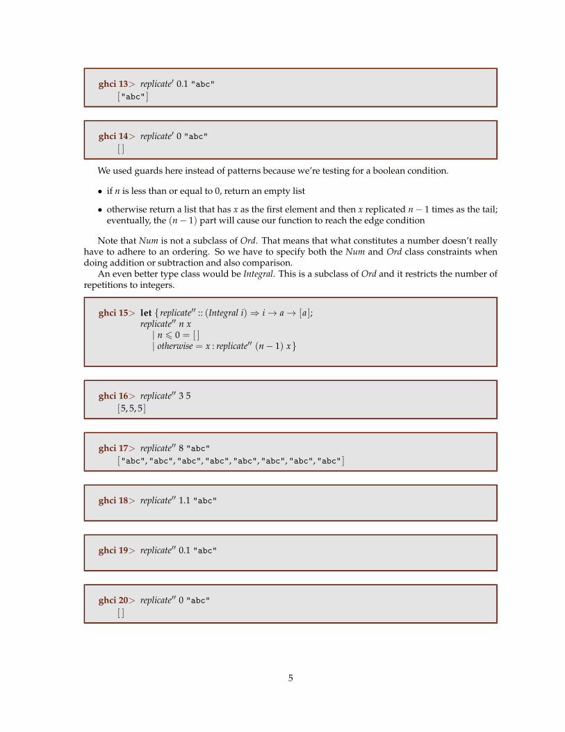
ghci 13> replicate′ 0.1 "abc"["abc" ]

ghci 14> replicate′ 0 "abc"[ ]

We used guards here instead of patterns because we’re testing for a boolean condition.

• if n is less than or equal to 0, return an empty list

• otherwise return a list that has x as the first element and then x replicated n− 1 times as the tail;eventually, the (n− 1) part will cause our function to reach the edge condition

Note that Num is not a subclass of Ord. That means that what constitutes a number doesn’t reallyhave to adhere to an ordering. So we have to specify both the Num and Ord class constraints whendoing addition or subtraction and also comparison.

An even better type class would be Integral. This is a subclass of Ord and it restricts the number ofrepetitions to integers.

ghci 15> let {replicate′′ :: (Integral i)⇒ i→ a→ [a ];replicate′′ n x| n 6 0 = [ ]| otherwise = x : replicate′′ (n− 1) x}

ghci 16> replicate′′ 3 5[5, 5, 5 ]

ghci 17> replicate′′ 8 "abc"["abc", "abc", "abc", "abc", "abc", "abc", "abc", "abc" ]

ghci 18> replicate′′ 1.1 "abc"

ghci 19> replicate′′ 0.1 "abc"

ghci 20> replicate′′ 0 "abc"[ ]

5

1.5 Recursion with multiple function arguments: Implementing take

Now we’ll implement take, which takes a certain number of elements from a list. For instance, take 3 [5,4, 3, 2, 1 ] will return [5, 4, 3 ].

There are 2 edge conditions: (i) if we try to take 0 or less elements from a list, we get an empty list;(ii) also, if we try to take anything from an empty list, we get an empty list. So let’s write it up:

ghci 21> let {take′ :: (Integral i)⇒ i→ [a ]→ [a ];take′ n | n 6 0 = [ ];take′ [ ] = [ ];take′ n (x : xs) = x : take′ (n− 1) xs}

• the first pattern specifies that if we try to take 0 or a negative number of elements, we get anempty list; we’re using to match the list because we don’t really care what it is in this case

– we use a guard, but without an otherwise part, so if n turns out to be more than 0, the match-ing will fall through to the next pattern

• the second pattern says that we get an empty list if we try to take anything from an empty list

• the third pattern breaks the list into a head and a tail; we state that taking n elements from a listequals a list that has x as the head prepended to a list that takes n− 1 elements from the tail

Optional homework: how does take 3 [6, 5, 4, 3, 2, 1 ] get evaluated? Write it down in full detail.

ghci 22> take′ 0 "hello"""

ghci 23> take′ 4 """"

ghci 24> take′ 4 "hello""hell"

ghci 25> take′ 4.2 "hello"

2 More practice examples

2.1 Implementing reverse

reverse simply reverses a list. The edge condition is the empty list: an empty list reversed equals theempty list itself. The recursive part: if we split a list into a head and a tail, the reversed list is equal tothe reversed tail and then the head at the end.

6

ghci 26> let {reverse′ :: [a ]→ [a ];reverse′ [ ] = [ ];reverse′ (x : xs) = reverse′ xs ++ [x ]}

ghci 27> reverse′ [ ][ ]

ghci 28> reverse′ "Hi""iH"

ghci 29> reverse′ "semaphore""erohpames"

2.2 Implementing repeat

repeat takes an element and returns an infinite list that just has that element. Here’s the recursiveimplementation of that:

ghci 30> let {repeat′ :: a→ [a ];repeat′ x = x : repeat′ x}

Calling repeat′ 3 will give us a list that starts with 3 and then has an infinite amount of 3’s as a tail:repeat′ 3 evaluates as 3 : repeat′ 3, which is 3 : (3 : repeat′ 3), which is 3 : (3 : (3 : repeat′ 3)) etc.

ghci 31> take 7 (repeat′ 3)[3, 3, 3, 3, 3, 3, 3 ]

repeat′ 3 will never finish evaluating, whereas take 7 (repeat′ 3) gives us a list of seven 3’s. Soessentially it’s like doing replicate 7 3.

2.3 Implementing zip

zip takes two lists and zips them together. E.g., zip [1, 2, 3 ] [’a’, ’b’ ] returns [ (1, ’a’), (2, ’b’) ] becauseit truncates the longer list to match the length of the shorter one.

How about if we zip something with an empty list? We get an empty list back. And this is our edgecondition. However, zip takes two lists as parameters, so there are actually two edge conditions.

ghci 32> let {zip′ :: [a ]→ [b ]→ [ (a, b) ];zip′ [ ] = [ ];zip′ [ ] = [ ];zip′ (x : xs) (y : ys) = (x, y) : zip′ xs ys}

7

The first two patterns say that if the first list or second list is empty, we get an empty list. The thirdone says that two lists zipped are equal to pairing up their heads and then tacking on the zipped tails.

ghci 33> zip′ [1 . . 3 ] [’a’, ’b’ ][ (1, ’a’), (2, ’b’) ]

Zipping [1, 2, 3 ] and [’a’, ’b’ ] will eventually try to zip [3 ] with [ ]. The edge condition patternskick in and so the result is (1, ’a’) : (2, ’b’) : [ ], which is the same as [ (1, ’a’), (2, ’b’) ].

2.4 Implementing elem

Let’s implement one more standard library function: elem. It takes an element and a list and sees ifthat element is in the list. The edge condition is the empty list, as it is most of the times with lists. Anempty list contains no elements, so it certainly doesn’t have the element we’re looking for.

ghci 34> let {elem′ :: (Eq a)⇒ a→ [a ]→ Bool;elem′ a [ ] = False;elem′ a (x : xs)| a ≡ x = True| otherwise = a ‘elem′‘ xs}

If the head isn’t the element then we check the tail. If we reach an empty list, the result is False.

ghci 35> elem′ 2 [1, 2, 5, 6 ]True

ghci 36> elem′ ’e’ "hello"True

ghci 37> elem′ ’r’ "hello"False

ghci 38> elem′ 2 "hello"

3 Quicksort

We have a list of items that can be sorted, i.e., their type is an instance of the Ord typeclass, and wewant to sort them. The quicksort algorithm has a very short and elegant implementation in Haskell,which is why quicksort has become somewhat of poster child for Haskell.

The type signature of our function is going to be quicksort :: (Ord a)⇒ [a ]→ [a ]. The edge conditionis the empty list, as expected: a sorted empty list is an empty list.

And here comes the main algorithm: a sorted list has all the values smaller than or equal to the headof the list in front (and those values are sorted), followed by the head of the list and then followed by

8

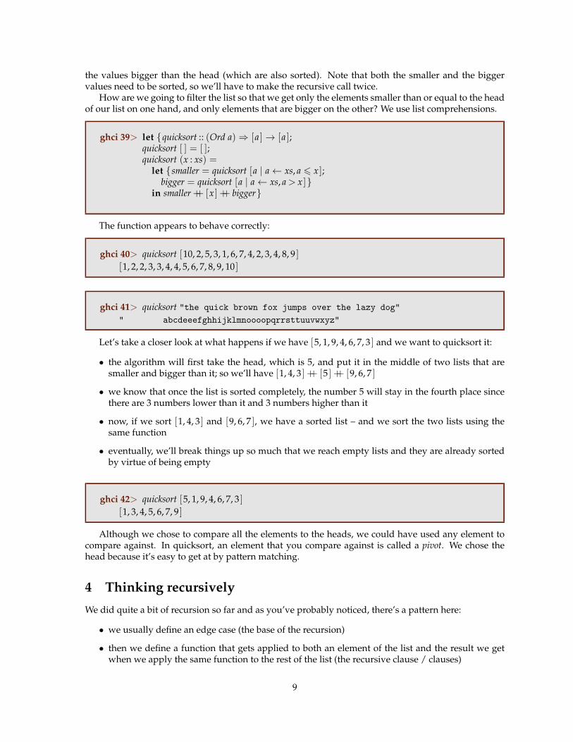
the values bigger than the head (which are also sorted). Note that both the smaller and the biggervalues need to be sorted, so we’ll have to make the recursive call twice.

How are we going to filter the list so that we get only the elements smaller than or equal to the headof our list on one hand, and only elements that are bigger on the other? We use list comprehensions.

ghci 39> let {quicksort :: (Ord a)⇒ [a ]→ [a ];quicksort [ ] = [ ];quicksort (x : xs) =

let {smaller = quicksort [a | a← xs, a 6 x ];bigger = quicksort [a | a← xs, a > x ]}

in smaller ++ [x ] ++ bigger}

The function appears to behave correctly:

ghci 40> quicksort [10, 2, 5, 3, 1, 6, 7, 4, 2, 3, 4, 8, 9 ][1, 2, 2, 3, 3, 4, 4, 5, 6, 7, 8, 9, 10 ]

ghci 41> quicksort "the quick brown fox jumps over the lazy dog"" abcdeeefghhijklmnoooopqrrsttuuvwxyz"

Let’s take a closer look at what happens if we have [5, 1, 9, 4, 6, 7, 3 ] and we want to quicksort it:

• the algorithm will first take the head, which is 5, and put it in the middle of two lists that aresmaller and bigger than it; so we’ll have [1, 4, 3 ] ++ [5 ] ++ [9, 6, 7 ]

• we know that once the list is sorted completely, the number 5 will stay in the fourth place sincethere are 3 numbers lower than it and 3 numbers higher than it

• now, if we sort [1, 4, 3 ] and [9, 6, 7 ], we have a sorted list – and we sort the two lists using thesame function

• eventually, we’ll break things up so much that we reach empty lists and they are already sortedby virtue of being empty

ghci 42> quicksort [5, 1, 9, 4, 6, 7, 3 ][1, 3, 4, 5, 6, 7, 9 ]

Although we chose to compare all the elements to the heads, we could have used any element tocompare against. In quicksort, an element that you compare against is called a pivot. We chose thehead because it’s easy to get at by pattern matching.

4 Thinking recursively

We did quite a bit of recursion so far and as you’ve probably noticed, there’s a pattern here:

• we usually define an edge case (the base of the recursion)

• then we define a function that gets applied to both an element of the list and the result we getwhen we apply the same function to the rest of the list (the recursive clause / clauses)

9

It doesn’t matter if we apply the function to a list, a tree or any other data structure. The basic structureof a recursive definition is the same:

• a sum is the first element of a list plus the sum of the rest of the list

• a product of a list is the first element of the list times the product of the rest of the list

• the length of a list is one plus the length of the tail of the list

• etc.

The edge case is usually a situation in which a recursive application doesn’t make sense:

• when dealing with lists, the edge case is most often the empty list

• when dealing with trees, the edge case is usually a terminal node (a node without daughters)

So when trying to think of a recursive way to solve a problem:

• think of when a recursive solution doesn’t apply and see if you can use that as an edge case

• think about how you’ll break the argument(s) of the function into subparts and on which partyou’ll use the recursive call

For example, a list is usually broken into a head and a tail by pattern matching and the recursive callis applied to the tail.

10