International Recessions

By Fabrizio Perri and Vincenzo Quadrini∗

September 2017

Macro developments leading up to the 2008 crisis displayed an unprecedented degree of interna-tional synchronization. Before the crisis all G7 countries experienced credit growth, and aroundthe time of the Lehman bankruptcy they all faced sharp and large contractions in both real andfinancial activity. Using a two-country model with financial frictions we show that a global liquid-ity shortage induced by pessimistic self-fulfilling expectations can quantitatively generate patternslike those observed in the data. The model also suggests that with more international financialintegration crises are less frequent but, when they hit, they are larger and more synchronizedacross countries.

Keywords: Credit shocks, global liquidity, international co-movement

JEL classification: F41, F44, G01

∗ Perri: Research Division, Federal Reserve Bank of Minneapolis, 90 Hennepin Avenue, Min-neapolis, MN 55480-0291 (email: fperri@umn.edu); Quadrini: Department of Finance and Busi-ness Economics, Marshall School of Business, University of Southern California, 701 ExpositionBoulevard, HOH 715, Los Angeles, CA 90089 (email: quadrini@usc.edu). We thank Mark Aguiarand three anonymous referees for excellent comments, Philippe Bacchetta, Ariel Burstein, FabioGhironi, Jean Imbs, Anastasios Karantounias, Thomas Laubach, Enrique Martınez-Garcıa, Do-minik Menno, Paolo Pesenti, Xavier Ragot, Etsuro Shioji, and Raf Wouters for thoughtfuldiscussions, and seminar participants at several institutions and conferences for very usefulcomments and suggestions. Perri acknowledges financial support from the European ResearchCouncil under Grant 313671. Quadrini acknowledges financial support from NSF Grant 1460013.The views expressed herein are those of the authors and not necessarily those of the FederalReserve Bank of Minneapolis or the Federal Reserve System. The authors declare that they haveno relevant or material financial interests that relate to the research described in this paper.

One of the most striking features of the 2008 crisis is that in the midst of it—during the

quarter following the Lehman bankruptcy—all major industrialized countries experienced ex-

traordinarily large and synchronized contractions in both real and financial aggregates. Moti-

vated by this evidence, we develop a simple theory of financial crises in open economies, aiming

to make two contributions. The first is to argue that the 2008 crisis could have been the result

of a global liquidity shortage induced by pessimistic self-fulfilling expectations. We do so by

showing that crisis patterns predicted by our theory are quantitatively consistent with many

features of the macro-economy observed before and during the 2008 crisis in the U.S. and other

G7 countries. The second contribution is to show how international financial integration affects

the probability and the size of crises. In particular with more international financial integra-

tion crises are less frequent but, when they hit, they are larger and more synchronized across

countries. This finding can have important normative implications, in light of the recent policy

debate on the desirability of capital markets integration.

Our analysis is based on a two-country model where firms in both countries use credit to

finance hiring and investment, and where the availability of credit depends on the value of

collateral, that is, the resale price of assets. The value of collateral is endogenous in the model

and depends on the market liquidity (access to credit) which in turn depends on the value

of collateral. This interdependence between the value of collateral and liquidity creates the

conditions for which the tightness of credit constraints can emerge endogenously as multiple

self-fulfilling equilibria.

In ‘good’ equilibria, the market expects high resale prices for the assets of defaulting firms,

which allows for looser borrowing constraints. As a result of the high borrowing capacity, firms

are not liquidity constrained and ex post there are firms with the required liquidity to purchase

the assets of defaulting firms. This keeps the resale price high and rationalizes, ex post, the ex

ante expectation of high collateral values. The higher availability of credit in good equilibria also

means that firms borrow more. As credit expands, however, a ‘bad’ equilibrium could emerge if

market expectations about the resale price of assets change and turn pessimistic. Expectations

of a low resale value implies that firms face tighter borrowing limits and are liquidity constrained.

Because firms are liquidity constrained, there are no firms capable of purchasing the assets of

defaulting firms and, as a result, the resale price is low. This rationalizes the expectation of

1

low prices, leading to ‘bad’ equilibria characterized by globally reduced credit, deleveraging,

and sharply depressed real activity. Financial integration implies that the prices of collateral

are equalized across countries, and hence credit conditions are also equalized. It is through

this mechanism that the crisis becomes global and displays a high degree of real and financial

synchronization.

The theory of endogenous financial booms and busts is important in two respects. First,

with endogenous credit shocks the model generates cross-country co-movement not only in real

variables but also in financial aggregates. To show this, we first study a version of the model in

which country-specific credit conditions change exogenously. If financial markets are integrated,

an exogenous tightening of credit in one country depresses employment and output in both

countries. However, while the country hit by the shock experiences a credit crunch, the other

country experiences a credit boom. Therefore, unless exogenous credit shocks are correlated

across countries, the model would not generate financial synchronization. We then show that

by making credit conditions endogenous, the model generates synchronized movements in both

real and financial variables. This result supports the view that a self-fulfilling, global liquidity

shortage, rather than isolated country-specific shocks, is important for understanding the 2008

crisis.

Second, the endogeneity of credit booms and busts allows us to assess how the probability

and depth of crises change when financial markets get more integrated. Since a self-fulfilling

crisis requires a high degree of coordination in expectations, the likelihood of coordination de-

creases when markets are integrated: an integrated market is a larger market that requires the

coordination of more agents. But as the probability of a crisis decreases, the incentive to lever-

age increases. Thus with integrated financial markets crises are less frequent, but their macro

consequences are bigger.

In the final part of the paper we evaluate the quantitative importance of liquidity induced

crises by calibrating the model to the United States and other G7 countries. The simulation

over the period 1995-2012 shows that the model captures several features of real and financial

data not only during the crisis but also in the period that preceded the crisis. The setup also

helps us understand a number of features that are hallmarks of financial crises in general. In

particular, the model generates (i) asymmetric dynamics of real variables in credit booms (slow

2

growth) and credit crashes (sharp contraction), (ii) countercyclical labor productivity, and (iii)

crises that are more severe when they arise after a long period of credit expansion. However,

the model does not capture the sluggish recovery after the crisis. This suggests that a liquidity

shortage can be responsible for the initial collapse in economic activity typical of a financial

crisis, but additional mechanisms are needed to understand the sluggish recovery that typically

follows the crisis.

One important observation concerning the international dimension of the recent crisis is

that employment was hit particularly hard in the United States but, at least initially, not in the

other G7 countries. Also, labor productivity did not change significantly in the United States

but declined in the other G7 countries. A related observation is that the ‘labor wedge’ increased

significantly in the United States but did not change substantially in other G7 countries (see, for

example, Ohanian 2010). Our baseline model with symmetric countries does not capture these

cross-country differences. However, in the extension with cross-country heterogeneity in labor

rigidities (more flexibility in the United States and less flexibility in other G7 countries), the

model can also generate the heterogeneous responses of employment, productivity, and labor

wedge.

The paper is related to the large literature on international co-movement. The literature

broadly focuses on two channels. The first is based on the existence of global or common shocks,

that is, exogenous disturbances that are correlated across countries. The second explanation

is based on the international transmission of country-specific shocks (for example through in-

vestment). In this paper, we show that credit shocks generate co-movement for both reasons:

exogenous credit shocks spill over from one country to the other, and endogenous credit shocks

will appear to the econometrician like a common shock or a global factor. Recent contributions

that analyze the role of financial markets for the international co-movement observed during the

2007-2009 crisis include Dedola and Lombardo (2010), Devereux and Yetman (2010), Devereux

and Sutherland (2011), Kollmann, Enders, and Muller (2011), and Kollmann (2013).

The role of credit shocks for macroeconomic fluctuations has been recently investigated pri-

marily in closed economy models.1 In this paper, instead, we study the international implications

1Examples are Guerrieri and Lorenzoni (2011), Gertler and Karadi (2011), Jermann and Quadrini (2012),

Goldberg (2013), Khan and Thomas (2013), Liu, Wang, and Zha (2013), Bacchetta, Benhima, and Poilly (2014),

and Christiano, Motto, and Rostagno (2014). There is also a long list of papers where the financial sector plays

3

of these shocks and provide a micro foundation based on self-fulfilling expectations. Our theory

is in line with the idea of liquidity crises resulting from multiple equilibria outcomes as dis-

cussed in Lucas and Stokey (2011) and it shares some similarities with models of bubbles as in

Kocherlakota (2009), Martin and Ventura (2012), and Miao and Wang (2017).

The idea that multiple equilibria can emerge in models in which the availability of credit

depends on the value of collateral assets has been first proposed by Shleifer and Vishny (1992)

and, more recently, by Benmelech and Bergman (2012) and Liu and Wang (2014). These studies,

however, consider only closed economy models. Our paper shows that multiple equilibria are

also important for capturing the international synchronization of recessions and their severity.

In this respect, it relates to the literature studying the sources of macroeconomic co-movement

and international transmission of shocks, starting with Backus, Kehoe, and Kydland (1992).

A recent study by Bacchetta and Van Wincoop (2016) also proposes a model with multiple

equilibria that generates international co-movement. The mechanism developed in their model

is based on self-fulfilling expectations about aggregate demand.

A central feature of our model is that financial constraints are ‘occasionally binding’. Men-

doza (2010), Bianchi (2011), and Bianchi and Mendoza (2013) also study economies with oc-

casionally binding constraints but do not investigate the issue of international co-movement.

Occasionally binding constraints are also central to Brunnermeier and Sannikov (2014) and

Arellano, Bai, and Kehoe (2012) but their analysis is limited to productivity shocks (level and

volatility) and to closed economies. Occasionally binding constraints are central to our setup

not only because they generate highly nonlinear dynamics but, more importantly, because they

are essential to generating multiple equilibria.

The paper is organized as follows. Section I documents some stylized facts about the crisis.

We then describe the theoretical framework starting in Section II with a simpler version of the

model without capital accumulation and exogenous credit shocks. After showing that exogenous

credit shocks do not generate co-movement in the flows of credit, we extend the model in Section

III to allow for multiple equilibria and endogenous credit shocks. In this section we also show

how financial integration affects the likelihood and depth of financial crises. Section IV adds

a role in the propagation of other nonfinancial shocks. Especially interesting are theories based on time-varying

uncertainty as in Arellano, Bai, and Kehoe (2012) and on interbank crises as in Boissay, Collard, and Smets

(2013).

4

capital accumulation and conducts the quantitative analysis. Section V concludes.

I Stylized Facts

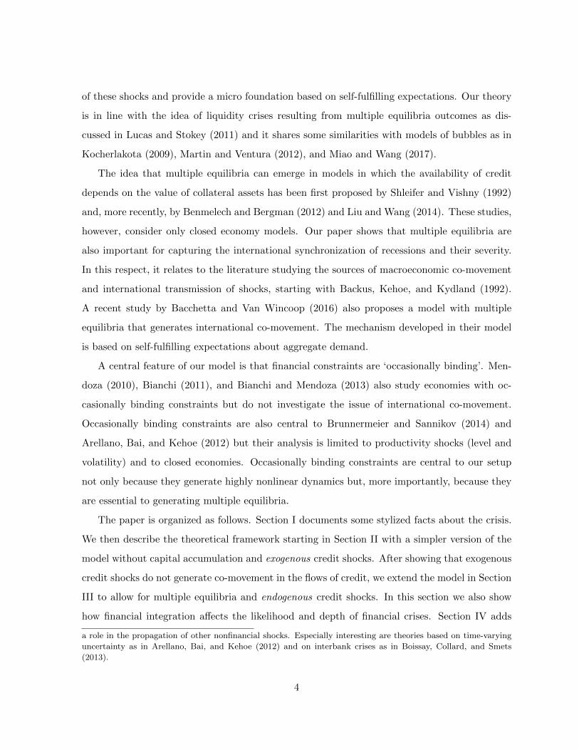
We now present some facts about international co-movement during the 2007-2009 crisis. Figure

1 plots the GDP dynamics for the G7 countries during the six most recent US recessions. In

each panel we plot, for each country, the percentage deviations from the level of GDP in the

quarter preceding the start of the US recession. Comparing the bottom right panel of the figure

with the other panels shows that the 2007-2009 recession and, in particular, the period following

the Lehman crisis, stands out in terms of both depth and macroeconomic synchronization. In

none of the previous recessions did GDP fall so much and in all countries.

Figure 1: Dynamics of GDP in the G7 countries during the six most recent US recessions

Note: All series normalized to 1 in the quarter preceding the start of the US recession (NBER recession dates).

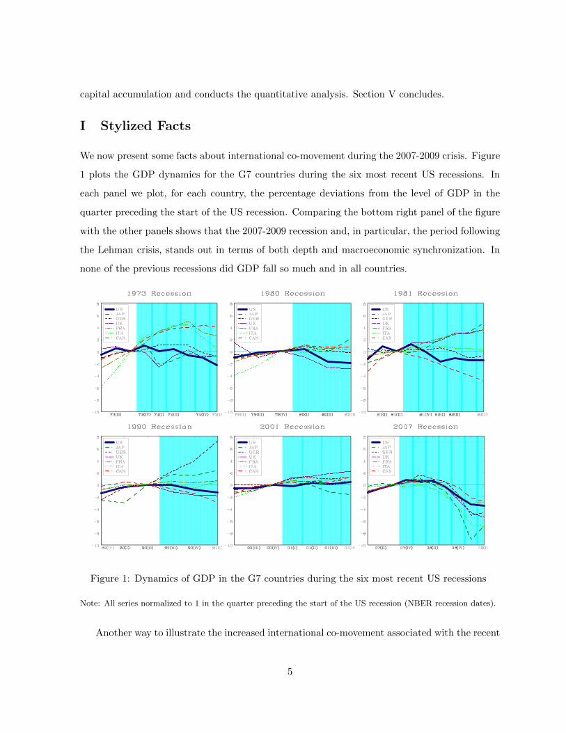
Another way to illustrate the increased international co-movement associated with the recent

5

crisis is provided in Figure 2. This figure plots the average bilateral correlations of 10-year rolling

windows of quarterly GDP growth between all G7 countries. Two standard deviation confidence

bands are also plotted. During the last two quarters of 2008 the average correlation jumped from

0.3 to 0.7 and the sample standard deviation fell significantly. This confirms that the 2007-2009

period stands out in the postwar era as a time of exceptional high co-movement for all developed

countries, a point also emphasized by Imbs (2010), among others.

Figure 2: Bilateral rolling correlations of GDP growth for G7 countries

Note: Each correlation is computed over a 10-year window of quarterly GDP growth. The x-axis is the most

recent date in the window. The vertical line denotes the third quarter of 2008 (Lehman’s bankruptcy).

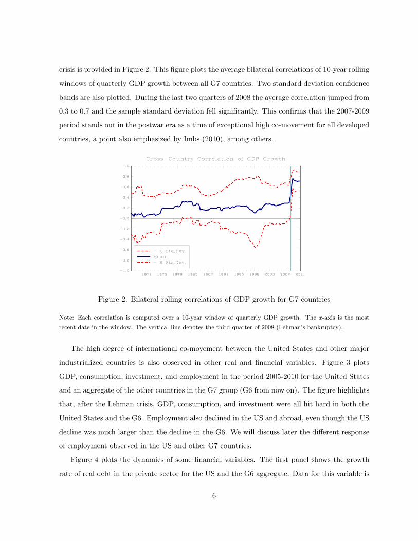
The high degree of international co-movement between the United States and other major

industrialized countries is also observed in other real and financial variables. Figure 3 plots

GDP, consumption, investment, and employment in the period 2005-2010 for the United States

and an aggregate of the other countries in the G7 group (G6 from now on). The figure highlights

that, after the Lehman crisis, GDP, consumption, and investment were all hit hard in both the

United States and the G6. Employment also declined in the US and abroad, even though the US

decline was much larger than the decline in the G6. We will discuss later the different response

of employment observed in the US and other G7 countries.

Figure 4 plots the dynamics of some financial variables. The first panel shows the growth

rate of real debt in the private sector for the US and the G6 aggregate. Data for this variable is

6

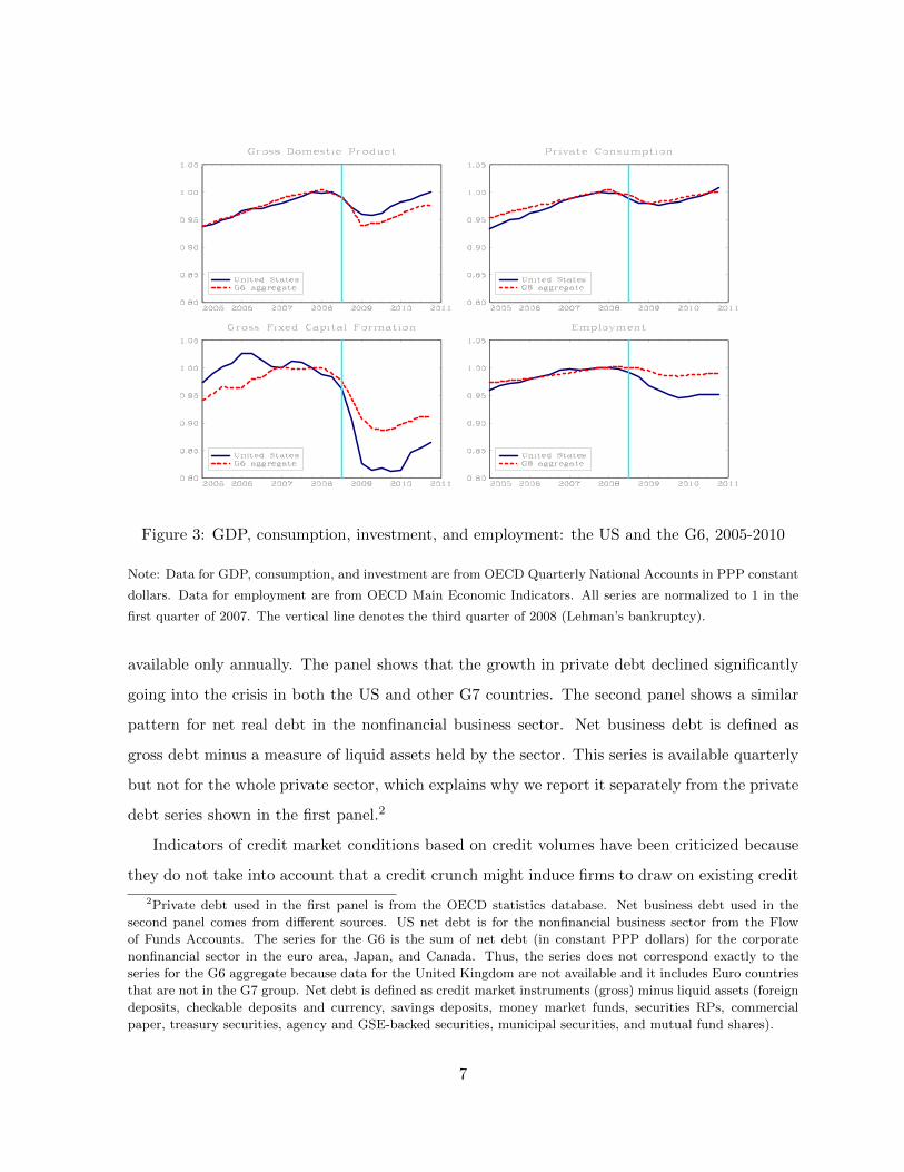
Figure 3: GDP, consumption, investment, and employment: the US and the G6, 2005-2010

Note: Data for GDP, consumption, and investment are from OECD Quarterly National Accounts in PPP constant

dollars. Data for employment are from OECD Main Economic Indicators. All series are normalized to 1 in the

first quarter of 2007. The vertical line denotes the third quarter of 2008 (Lehman’s bankruptcy).

available only annually. The panel shows that the growth in private debt declined significantly

going into the crisis in both the US and other G7 countries. The second panel shows a similar

pattern for net real debt in the nonfinancial business sector. Net business debt is defined as

gross debt minus a measure of liquid assets held by the sector. This series is available quarterly

but not for the whole private sector, which explains why we report it separately from the private

debt series shown in the first panel.2

Indicators of credit market conditions based on credit volumes have been criticized because

they do not take into account that a credit crunch might induce firms to draw on existing credit

2Private debt used in the first panel is from the OECD statistics database. Net business debt used in the

second panel comes from different sources. US net debt is for the nonfinancial business sector from the Flow

of Funds Accounts. The series for the G6 is the sum of net debt (in constant PPP dollars) for the corporate

nonfinancial sector in the euro area, Japan, and Canada. Thus, the series does not correspond exactly to the

series for the G6 aggregate because data for the United Kingdom are not available and it includes Euro countries

that are not in the G7 group. Net debt is defined as credit market instruments (gross) minus liquid assets (foreign

deposits, checkable deposits and currency, savings deposits, money market funds, securities RPs, commercial

paper, treasury securities, agency and GSE-backed securities, municipal securities, and mutual fund shares).

7

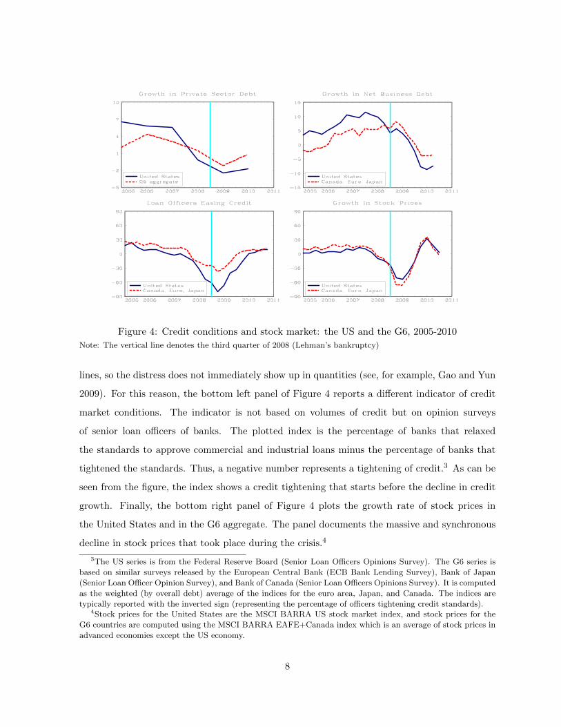
Figure 4: Credit conditions and stock market: the US and the G6, 2005-2010

Note: The vertical line denotes the third quarter of 2008 (Lehman’s bankruptcy)

lines, so the distress does not immediately show up in quantities (see, for example, Gao and Yun

2009). For this reason, the bottom left panel of Figure 4 reports a different indicator of credit

market conditions. The indicator is not based on volumes of credit but on opinion surveys

of senior loan officers of banks. The plotted index is the percentage of banks that relaxed

the standards to approve commercial and industrial loans minus the percentage of banks that

tightened the standards. Thus, a negative number represents a tightening of credit.3 As can be

seen from the figure, the index shows a credit tightening that starts before the decline in credit

growth. Finally, the bottom right panel of Figure 4 plots the growth rate of stock prices in

the United States and in the G6 aggregate. The panel documents the massive and synchronous

decline in stock prices that took place during the crisis.4

3The US series is from the Federal Reserve Board (Senior Loan Officers Opinions Survey). The G6 series is

based on similar surveys released by the European Central Bank (ECB Bank Lending Survey), Bank of Japan

(Senior Loan Officer Opinion Survey), and Bank of Canada (Senior Loan Officers Opinions Survey). It is computed

as the weighted (by overall debt) average of the indices for the euro area, Japan, and Canada. The indices are

typically reported with the inverted sign (representing the percentage of officers tightening credit standards).4Stock prices for the United States are the MSCI BARRA US stock market index, and stock prices for the

G6 countries are computed using the MSCI BARRA EAFE+Canada index which is an average of stock prices in

advanced economies except the US economy.

8

The key lesson we learn from Figure 4 is that, right around 2008, credit conditions moved

from strongly loose to strongly tight both in the United States and in the G6 countries.

A final observation relates to the asymmetry between real and financial variables in the

expansion phase before the crisis and the collapse during the crisis. The top left panel of Figure

4 shows that, in the years preceding the crisis, debt experienced significant growth. Figure 3,

instead, shows that the growth in real variables has been moderate. During the crisis period,

however, all variables, both real and financial, contracted sharply. This feature is not unique to

the 2007-2009 financial crisis. Several authors have observed that many historical episodes of

credit booms are not associated with much faster growth in real economic activity. However,

when a credit boom experiences a sudden stop, the reversal is often characterized by sharp

macroeconomic contractions. See, for example, Reinhart and Rogoff (2009), Claessens, Kose,

and Terrones (2011), and Schularick and Taylor (2012).

The facts presented in this section—high international co-movement in real and financial

variables during the crisis, large employment (for the United States), and asymmetry between

the precrisis phase and the crisis phase—cannot be easily explained with a standard workhorse

international business cycle model. In the next sections we propose a theoretical framework

with endogenous credit shocks that helps us understand these facts.

II Model with Exogenous Credit Shocks

We start with a simple model without capital accumulation and with exogenous credit shocks.

The model provides intuition for the key financial mechanism through which changes in the

availability of credit affect employment and the real sector of the economy. However, while the

model generates cross-country co-movements in real variables in response to credit shocks, it

does not generate co-movement in financial aggregates. We will then extend the setup with

endogenous credit shocks which allow the model to generate co-movement also in financial

variables.

There are two types of atomistic agents: a mass 1 of workers and a mass ω of investors. The

relative sizes of workers and investors are irrelevant for the equilibrium properties of the model

but will affect the computation of the welfare consequences of financial integration which we will

9

report later in the paper. Only investors have access to the ownership of firms whereas workers

can only save in the form of bonds (market segmentation). Investors and workers have different

discount factors: β for investors and δ > β for workers. As we will see, the different discounting

implies that in equilibrium firms borrow from workers.5 To facilitate the presentation we describe

first the closed-economy version of the model.

A Investors and Firms

Investors have lifetime utility E0∑∞

t=0 βtu(ct). They are the owners of firms and can trade

shares with other investors. We assume that the mass of firms is fixed and equal to 1. Denoting

by nt the shares of firms held by an individual investor, Dt the aggregate dividends paid by all

firms, and Pt the ex-dividend price of shares, the problem solved by an investor can be written

recursively as

Ω(st, nt) = maxct,nt+1

u(ct) + βEtΩ(st+1, nt+1)

(1)

subject to:

nt(Dt + Pt) = ct + nt+1Pt,

where Ω(st, nt) is the value function for the investor which depends on the aggregate states st

(defined later) and the shares of firms nt (individual state). We are assuming that investors do

not borrow or save in the form of bonds.

The first order conditions for the investor’s problem return the typical Euler equation

uc(ct)Pt = βEtuc(ct+1)(Dt +Pt), where the subscript in the utility function denotes derivatives.

Investors are homogeneous and they earn only dividend incomes. Therefore, in equilibrium we

have nt = nt+1 = 1/ω and ct = Dt/ω, where ω has been defined earlier as the fixed mass of

investors (while the mass of firms is 1). We can then express the equilibrium price of a share as

Pt = βEt[uc(Dt+1/ω)/uc(Dt/ω)](Dt+1 + Pt+1). This shows that investors discount future divi-

5Several mechanisms have been proposed in the literature to generate a borrowing incentive for firms: tax

deductability of interests, uninsurable idiosyncratic risks for lenders, bargaining of wages, and so on. Since the

specific mechanism that leads to the pecking order of debt is not important for our results, we simply assume

different discounting as in Kiyotaki and Moore (1997).

10

dends by mt+1 = βuc(Dt+1/ω)/uc(Dt/ω). Since firms operate on behalf of investors, this will

also be the discount factor used by firms. In what follows we assume that the utility of investors

takes the CES form so that ω cancels out. The discount factor is then mt+1 = βuc(Dt+1)/uc(Dt).

Firms operate the production function F (ht) = khνt , where k is the ‘fixed’ input of capital,

ht is the variable input of labor, and ν < 1 implying decreasing returns in the variable input.

Firms start the period with intertemporal debt bt. Before producing, they choose labor

input ht, dividends dt, and next period debt bt+1. We use the small letter dt to denote the

dividends paid by an ‘individual’ firm while in the investor’s problem we used the capital letter

Dt to denote the ‘aggregate’ dividends paid by all firms. Whenever necessary, we will use

this notation throughout the paper (small letters for individual variables and capital letters for

aggregate variables). Denoting by Rt is the gross interest rate, the budget constraint is

(2) bt + wtht + dt = F (ht) +bt+1

Rt.

The payments of wages, wtht, dividends, dt, and current debt net of the new issue, bt −bt+1/Rt, are made before the realization of revenues. Thus, the firm faces a cash flow mismatch.

To cover the cash mismatch, the firm contracts the intraperiod loan xt = wtht+dt+bt−bt+1/Rt,

which is repaid at the end of the period after the realization of revenues.6 Using the budget

constraint (2), we can see that the intraperiod loan is equal to the revenue, that is, xt = F (ht).

Debt contracts are not perfectly enforceable because firms can default. Default takes place

at the end of the period before repaying the intraperiod loan. At this stage, a firm holds the

revenue F (ht) which can be diverted. If the firm defaults, the lender has the right to liquidate

its assets. However, after the diversion of F (ht), the only remaining asset is the physical capital

k. Suppose that the liquidation value of capital is ξtk, where ξt is stochastic. Then, to ensure

that the firm does not default, the lender imposes the enforcement constraint

(3) xt +bt+1

Rt≤ ξtk.

The left-hand side terms are the total liabilities of the firm at the end of the period (intrape-

riod and intertemporal). The right-hand side term is the liquidation value of firm’s capital. The

6As an alternative we could assume that firms cannot borrow with intraperiod loans but they can carry cash

from the previous period. In this case, firms would carry cash since this is the only way to make the payments

before the realization of revenues. The explicit consideration of cash would not change the key properties of the

model but would complicate the numerical solution because it adds another state variable.

11

constraint is derived under the assumption that the firm has the whole bargaining power in the

renegotiation of the debt as in Hart and Moore (1994) and can distribute the diverted liquidity

as dividends to shareholders. The formal derivation is provided in Appendix A.

To illustrate the role played by fluctuations in ξt, consider a preshock equilibrium in which

the enforcement constraint is binding. Starting from this equilibrium, suppose that ξt decreases.

This forces the firm to reduce either the dividends, the input of labor, or both.

To see why, let’s start with the assumption that the firm does not change the input of labor ht.

This implies that the intraperiod loan also does not change because xt = wtht+dt+bt−bt+1/Rt =

F (ht). Consequently, the only way to satisfy the enforcement constraint (3) is by reducing the

intertemporal debt bt+1. We can then see from the budget constraint (2) that the reduction in

bt+1 requires a reduction in dividends. Thus, the firm is forced to substitute debt with equity.

Alternatively, the firm could keep the dividends unchanged and reduce the intraperiod loan

xt = F (ht). This would also ensure that the enforcement constraint is satisfied but it requires

the reduction in the input of labor. Therefore, after a reduction in ξt, the firm faces a trade-off:

paying lower dividends or cutting employment. The optimal choice depends on the relative cost

of changing these two margins, which, as we will see, depends on the stochastic discount factor

mt+1 = βuc(dt+1)/uc(dt).7

Firm’s Problem: The optimization problem of the firm can be written recursively as

V (st; bt) = maxdt,ht,bt+1

dt + Etmt+1V (st+1; bt+1)

(4)

subject to:

bt + dt = F (ht)− wtht +bt+1

Rt(5)

F (ht) +bt+1

Rt≤ ξtk,(6)

where st are the aggregate states (as specified below).

7Movements in ξt are consistent with Eisfeldt and Rampini (2006) who suggest that the liquidity of capital

must be procyclical in order to match the observed reallocation.

12

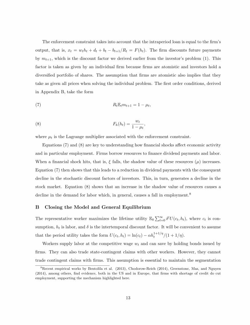
The enforcement constraint takes into account that the intraperiod loan is equal to the firm’s

output, that is, xt = wtht + dt + bt − bt+1/Rt = F (ht). The firm discounts future payments

by mt+1, which is the discount factor we derived earlier from the investor’s problem (1). This

factor is taken as given by an individual firm because firms are atomistic and investors hold a

diversified portfolio of shares. The assumption that firms are atomistic also implies that they

take as given all prices when solving the individual problem. The first order conditions, derived

in Appendix B, take the form

RtEtmt+1 = 1− µt,(7)

Fh(ht) =wt

1− µt,(8)

where µt is the Lagrange multiplier associated with the enforcement constraint.

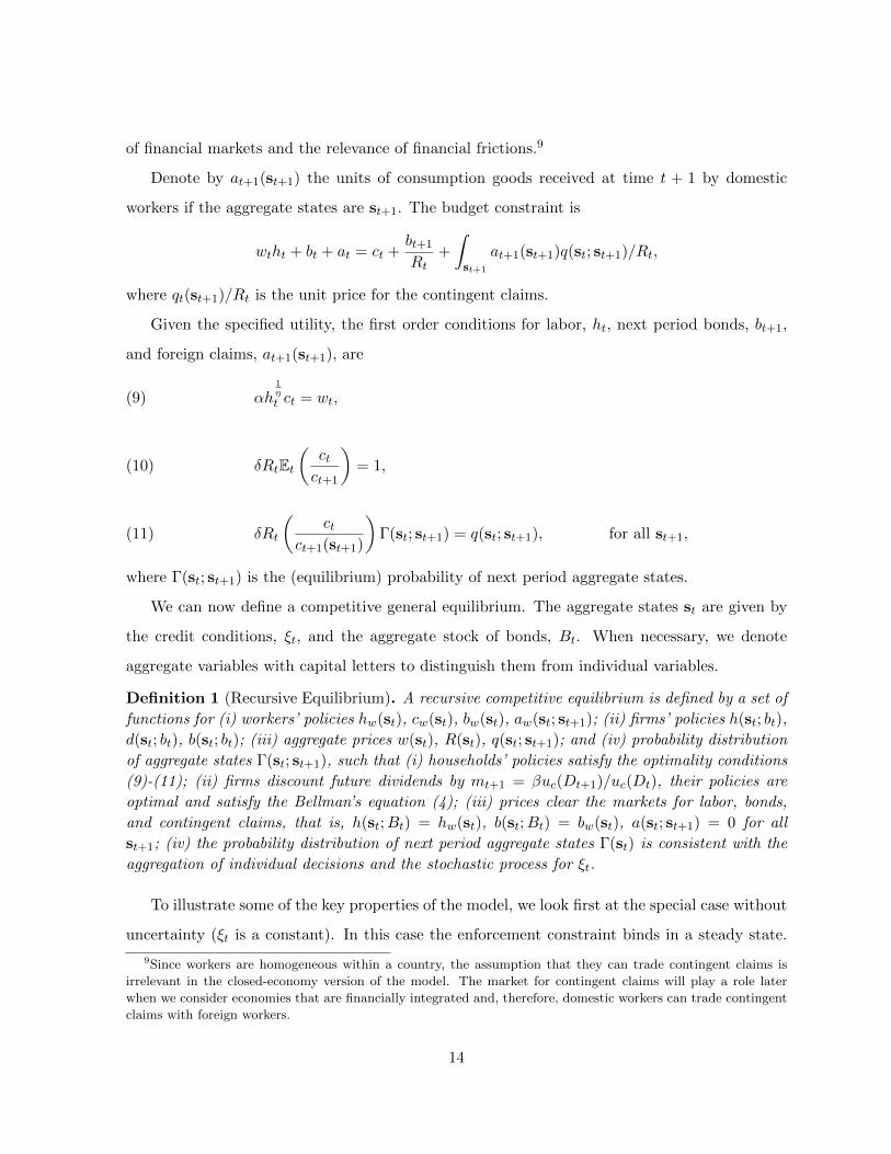
Equations (7) and (8) are key to understanding how financial shocks affect economic activity

and in particular employment. Firms borrow resources to finance dividend payments and labor.

When a financial shock hits, that is, ξ falls, the shadow value of these resources (µ) increases.

Equation (7) then shows that this leads to a reduction in dividend payments with the consequent

decline in the stochastic discount factors of investors. This, in turn, generates a decline in the

stock market. Equation (8) shows that an increase in the shadow value of resources causes a

decline in the demand for labor which, in general, causes a fall in employment.8

B Closing the Model and General Equilibrium

The representative worker maximizes the lifetime utility E0∑∞

t=0 δtU(ct, ht), where ct is con-

sumption, ht is labor, and δ is the intertemporal discount factor. It will be convenient to assume

that the period utility takes the form U(ct, ht) = ln(ct)− αh1+1/ηt /(1 + 1/η).

Workers supply labor at the competitive wage wt and can save by holding bonds issued by

firms. They can also trade state-contingent claims with other workers. However, they cannot

trade contingent claims with firms. This assumption is essential to maintain the segmentation

8Recent empirical works by Bentolila et al. (2013), Chodorow-Reich (2014), Greenstone, Mas, and Nguyen

(2014), among others, find evidence, both in the US and in Europe, that firms with shortage of credit do cut

employment, supporting the mechanism highlighted here.

13

of financial markets and the relevance of financial frictions.9

Denote by at+1(st+1) the units of consumption goods received at time t + 1 by domestic

workers if the aggregate states are st+1. The budget constraint is

wtht + bt + at = ct +bt+1

Rt+

∫st+1

at+1(st+1)q(st; st+1)/Rt,

where qt(st+1)/Rt is the unit price for the contingent claims.

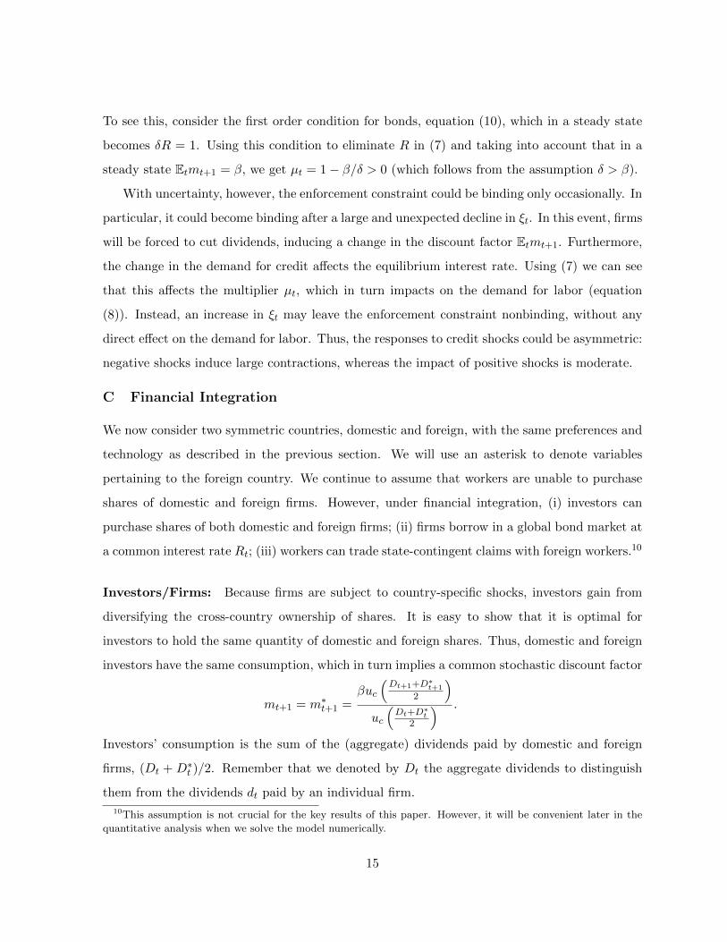
Given the specified utility, the first order conditions for labor, ht, next period bonds, bt+1,

and foreign claims, at+1(st+1), are

αh1η

t ct = wt,(9)

δRtEt(

ctct+1

)= 1,(10)

δRt

(ct

ct+1(st+1)

)Γ(st; st+1) = q(st; st+1), for all st+1,(11)

where Γ(st; st+1) is the (equilibrium) probability of next period aggregate states.

We can now define a competitive general equilibrium. The aggregate states st are given by

the credit conditions, ξt, and the aggregate stock of bonds, Bt. When necessary, we denote

aggregate variables with capital letters to distinguish them from individual variables.

Definition 1 (Recursive Equilibrium). A recursive competitive equilibrium is defined by a set of

functions for (i) workers’ policies hw(st), cw(st), bw(st), aw(st; st+1); (ii) firms’ policies h(st; bt),

d(st; bt), b(st; bt); (iii) aggregate prices w(st), R(st), q(st; st+1); and (iv) probability distribution

of aggregate states Γ(st; st+1), such that (i) households’ policies satisfy the optimality conditions

(9)-(11); (ii) firms discount future dividends by mt+1 = βuc(Dt+1)/uc(Dt), their policies are

optimal and satisfy the Bellman’s equation (4); (iii) prices clear the markets for labor, bonds,

and contingent claims, that is, h(st;Bt) = hw(st), b(st;Bt) = bw(st), a(st; st+1) = 0 for all

st+1; (iv) the probability distribution of next period aggregate states Γ(st) is consistent with the

aggregation of individual decisions and the stochastic process for ξt.

To illustrate some of the key properties of the model, we look first at the special case without

uncertainty (ξt is a constant). In this case the enforcement constraint binds in a steady state.

9Since workers are homogeneous within a country, the assumption that they can trade contingent claims is

irrelevant in the closed-economy version of the model. The market for contingent claims will play a role later

when we consider economies that are financially integrated and, therefore, domestic workers can trade contingent

claims with foreign workers.

14

To see this, consider the first order condition for bonds, equation (10), which in a steady state

becomes δR = 1. Using this condition to eliminate R in (7) and taking into account that in a

steady state Etmt+1 = β, we get µt = 1− β/δ > 0 (which follows from the assumption δ > β).

With uncertainty, however, the enforcement constraint could be binding only occasionally. In

particular, it could become binding after a large and unexpected decline in ξt. In this event, firms

will be forced to cut dividends, inducing a change in the discount factor Etmt+1. Furthermore,

the change in the demand for credit affects the equilibrium interest rate. Using (7) we can see

that this affects the multiplier µt, which in turn impacts on the demand for labor (equation

(8)). Instead, an increase in ξt may leave the enforcement constraint nonbinding, without any

direct effect on the demand for labor. Thus, the responses to credit shocks could be asymmetric:

negative shocks induce large contractions, whereas the impact of positive shocks is moderate.

C Financial Integration

We now consider two symmetric countries, domestic and foreign, with the same preferences and

technology as described in the previous section. We will use an asterisk to denote variables

pertaining to the foreign country. We continue to assume that workers are unable to purchase

shares of domestic and foreign firms. However, under financial integration, (i) investors can

purchase shares of both domestic and foreign firms; (ii) firms borrow in a global bond market at

a common interest rate Rt; (iii) workers can trade state-contingent claims with foreign workers.10

Investors/Firms: Because firms are subject to country-specific shocks, investors gain from

diversifying the cross-country ownership of shares. It is easy to show that it is optimal for

investors to hold the same quantity of domestic and foreign shares. Thus, domestic and foreign

investors have the same consumption, which in turn implies a common stochastic discount factor

mt+1 = m∗t+1 =βuc

(Dt+1+D∗t+1

2

)uc

(Dt+D∗t

2

) .

Investors’ consumption is the sum of the (aggregate) dividends paid by domestic and foreign

firms, (Dt + D∗t )/2. Remember that we denoted by Dt the aggregate dividends to distinguish

them from the dividends dt paid by an individual firm.

10This assumption is not crucial for the key results of this paper. However, it will be convenient later in the

quantitative analysis when we solve the model numerically.

15

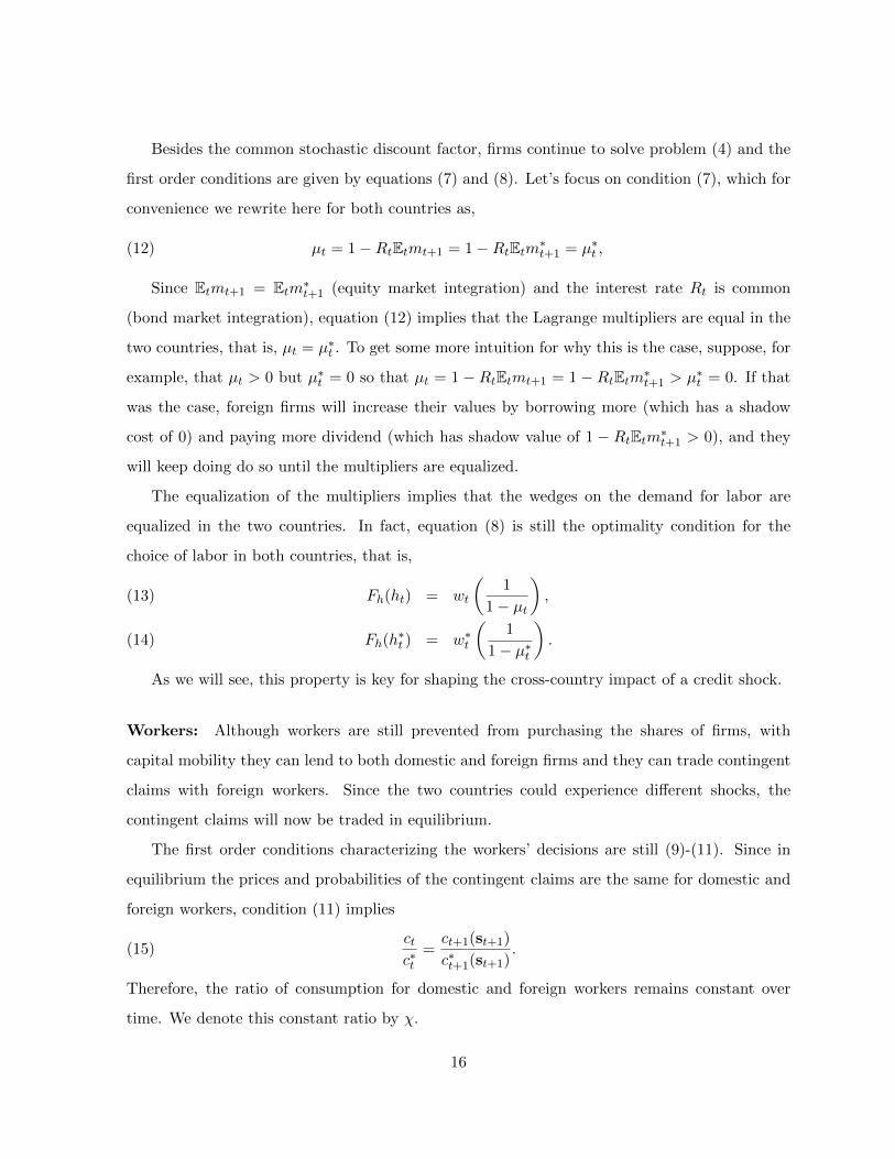
Besides the common stochastic discount factor, firms continue to solve problem (4) and the

first order conditions are given by equations (7) and (8). Let’s focus on condition (7), which for

convenience we rewrite here for both countries as,

(12) µt = 1−RtEtmt+1 = 1−RtEtm∗t+1 = µ∗t ,

Since Etmt+1 = Etm∗t+1 (equity market integration) and the interest rate Rt is common

(bond market integration), equation (12) implies that the Lagrange multipliers are equal in the

two countries, that is, µt = µ∗t . To get some more intuition for why this is the case, suppose, for

example, that µt > 0 but µ∗t = 0 so that µt = 1− RtEtmt+1 = 1− RtEtm∗t+1 > µ∗t = 0. If that

was the case, foreign firms will increase their values by borrowing more (which has a shadow

cost of 0) and paying more dividend (which has shadow value of 1 − RtEtm∗t+1 > 0), and they

will keep doing do so until the multipliers are equalized.

The equalization of the multipliers implies that the wedges on the demand for labor are

equalized in the two countries. In fact, equation (8) is still the optimality condition for the

choice of labor in both countries, that is,

Fh(ht) = wt

(1

1− µt

),(13)

Fh(h∗t ) = w∗t

(1

1− µ∗t

).(14)

As we will see, this property is key for shaping the cross-country impact of a credit shock.

Workers: Although workers are still prevented from purchasing the shares of firms, with

capital mobility they can lend to both domestic and foreign firms and they can trade contingent

claims with foreign workers. Since the two countries could experience different shocks, the

contingent claims will now be traded in equilibrium.

The first order conditions characterizing the workers’ decisions are still (9)-(11). Since in

equilibrium the prices and probabilities of the contingent claims are the same for domestic and

foreign workers, condition (11) implies

(15)ctc∗t

=ct+1(st+1)

c∗t+1(st+1).

Therefore, the ratio of consumption for domestic and foreign workers remains constant over

time. We denote this constant ratio by χ.

16

Aggregate States and Equilibrium: In the economy with integrated financial markets, the

aggregate states are st = (ξt, ξ∗t , Bt, B

∗t , At), where Bt and B∗t represent the aggregate financial

liabilities of firms, and At is the aggregate foreign asset position of the domestic country.

The definition of equilibria is analogous to the one provided for the closed economy with

some minor adjustments. In particular, we need to take into account that the bond market is

global and there is a common discount factor for domestic and foreign firms.

Denote by Wt = Bt + B∗t the worldwide wealth of households/workers. This is the sum

of bonds issued by domestic firms, Bt, and foreign firms, B∗t . Because the consumption ratio

of domestic and foreign workers is constant at χ and the employment policy of firms does not

depend on the individual debt but only on the worldwide debt, the recursive equilibrium can be

characterized by the state vector st = (ξt, ξ∗t ,Wt). Therefore, the assumption of cross-country

risk sharing within workers (with the trade of state-contingent claims) and within investors (with

the ownership of foreign shares) allows us to reduce the number of endogenous states to only

one variable, Wt.

Intuitively, to characterize the firms’ policies we do not need to know the distribution of

liabilities between domestic and foreign firms. We only need to know the worldwide debt, which

is equal to Wt. Since investors own an internationally diversified portfolio of shares, effectively

there is only one representative global investor. This is similar to a representative firm with two

productive units: one unit located in the domestic country and the other in the foreign country.

Since both units have a common owner, it does not matter how the debt is distributed between

the two units. What matters for investors is the total debt and the total dividends.11

The Effects of a Credit Shock: The next proposition characterizes the real impact of a

country-specific credit shock when financial markets are integrated.

Proposition 1. An unexpected change in ξt (domestic credit shock) has the same impact on

employment and output of domestic and foreign countries.

Proof. We have already shown that the Lagrange multiplier µt is equalized across countries. If

the ratio of wages in the two countries does not change, the first order conditions imply that all

11This is similar to the problem of a multinational firm that faces demand uncertainty in different countries as

studied in Goldberg and Kolstad (1995). There are also some similarities with the problem of a multinational bank

with foreign subsidiaries. Cetorelli and Goldberg (2012) provide evidence that multinational banks do reallocate

financial resources internally in response to country-specific shocks.

17

firms choose the same employment. To complete the proof we have to show that the cross-country

wage ratio stays constant. Because firms in both countries have the same demand for labor and

the ratio of workers’ consumption remains constant, the first order condition for the supply of

labor, equation (9), implies that the ratio of wages does not change.

Thus, the model generates cross-country co-movement in real economic activities even if

shocks are not correlated across countries. However, the model does not generate co-movement

in financial flows as a negative credit shock in the domestic country generates a credit crunch

only in this country while the foreign country could experience a credit boom.

To understand why a negative credit shock in one country generates a credit boom in the

other, consider an initial equilibrium in which the enforcement constraint is not binding in either

country. Starting from this equilibrium, suppose that only the domestic economy is hit by a

negative credit shock (a reduction in ξt but not in ξ∗t ), and this induces binding enforcement

constraints in both countries. When ξt falls in the domestic country, the shadow value of credit

increases in both countries. However, since the constraint has not changed for foreign firms,

they will take more credit. In other words, foreign firms increase their borrowing to pay more

dividends and offset, partially, the reduction in dividends from firms in the domestic country.

We conclude this section by summarizing the main results obtained so far. In a regime with

capital mobility, the model generates a high degree of co-movement in real variables in response

to country-specific credit shocks. However, unless these shocks are correlated, the model does

not generate co-movement in financial aggregates, which is also a distinguished feature of the

2008 crisis. In the next section we will make credit shocks endogenous providing a theory for

time variations in credit tightness and cross-country co-movement in financial aggregates.

III Endogenous Credit Shocks

We now interpret ξt and ξ∗t as the endogenous prices at which capital can be sold if a firm

defaults and its capital is liquidated.

In case of liquidation, the capital of the firm k is perfectly divisible, but before it can be reused

it needs to be sold to competitive intermediaries which, after paying a per-unit intermediation

cost, can resell it to potential final buyers.12 If financial markets are integrated, the capital can

12Even though households are creditors of firms, when a firm defaults they still need the service of these

18

be sold to domestic and foreign buyers. Both workers and other firms could buy the liquidated

capital and transform it one-to-one in consumption goods. Therefore, the maximum price that

buyers are willing to pay for one unit of capital is 1. The structure of the market for liquidated

capital is characterized by two assumptions.

Assumption 1. The per-unit intermediation cost, denoted by Φ(Nt), is a function of the mass

of buyers Nt (workers and firms). The cost is strictly decreasing in Nt ∈ [0, 2] and satisfies

Φ(1) = 1− ξ and Φ(2) = 1− ξ ≥ 0.

Since there is a unit mass of workers and a unit mass of firms, the maximum mass of buyers

is 2. Therefore, Nt ∈ [0, 2] is the relevant interval for the function Φ(Nt). At the heart of the

above assumption is the empirical observation by Eisfeldt and Rampini (2006) that secondary

markets for capital work less efficiently in bad times. It could be micro-founded with matching

frictions and increasing returns in the matching technology, in the spirit of Diamond (1982).13

Denote by ξt the price paid by intermediaries to purchase one unit of capital from liquidated

firms. This is the ‘liquidation’ price for firms. Furthermore, denote by ξbt the price at which

intermediaries resell the purchased capital. Since the intermediation sector is competitive, in

equilibrium we have ξbt = ξt + Φ(Nt). Therefore, the price ξbt is always bigger than ξt. The

difference, however, declines if the number of potential buyers Nt increases. The next assumption

provides the conditions for participating in the market for liquidated capital.

Assumption 2. Buyers can purchase liquidated capital from the intermediaries only if their

borrowing constraints are slack.

This assumption is justified by limited enforcement, as we did for the enforcement constraint

(3), and by the assumption that the purchase of capital requires credit (i.e., the firm receives

resources only after production). If the enforcement constraint is binding, the firm simply cannot

specialized firms (intermediaries) to liquidate the capital. This assumption is necessary to generate an endogenous

(and varying across equilibria) resale price of capital.13A sketch of the matching frictions that could lead to similar properties is as follows. Suppose that an

intermediary finds a buyer with probability 1−Ψ(N), where N is the number of potential buyers, and Ψ′(N) < 0.

If the intermediary does not find a buyer, capital fully depreciates. The intermediary would then maximize

[1 − Ψ(N)]ξbk − ξk, where ξb is the price paid by the buyer and ξ is the price paid by the intermediary to

the seller. Competition implies that in equilibrium [1 − Ψ(N)]ξb = ξ. Furthermore, since buyers can transform

one unit of capital into one unit of consumption, ξb = 1. Assuming that Ψ′(N) < 0, i.e., increasing returns to

scale in the matching technology, could generate multiple equilibria. The increasing transaction cost assumed

in Assumption 1 captures, in reduced form, the increasing returns to scale in the matching technology. We are

grateful to an anonymous referee for outlining the matching environment described in this footnote.

19

get financing to buy additional capital. However, if the constraint is not binding, the firm can

increase its borrowing and buy liquidated capital. This is why only buyers with nonbinding

borrowing constraints can participate in the market for liquidated capital.

Since workers do not face binding constraints (in fact workers are lenders not borrowers),

they can always participate in the market for liquidated capital. Firms, on the other hand, could

face binding constraints, in which case they are unable to participate. We will refer to a firm

with a nonbinding borrowing constraint as liquid.

Lemma 1. In equilibrium ξbt = 1 and the liquidation price is ξt = 1− Φ(Nt).

Proof. Since buyers can transform one unit of capital to one unit of consumption goods, the

maximum price they are willing to pay is 1. In equilibrium workers always participate while no

capital is never sold. Since the demand for liquidated capital is bigger than the supply, ξbt = 1.

Perfect competition implies that intermediaries make zero profits in equilibrium and, therefore,

ξbt = ξt + Φ(Nt). We have already shown that ξbt = 1 and, therefore, the zero profit condition

implies ξt = 1− Φ(Nt).

To clarify the role of liquidity, we should think of a period as divided in two subperiods:

beginning-of-period and end-of-period. Operational decisions are made at the beginning of the

period while default decisions and potential sales of liquidated capital take place at the end of

the period.

1. Beginning-of-period: Agents form expectations ξet for the price at which liquidated

capital could be sold at the end of the period. Given the expected price, firms make

all operational decisions including the input of labor ht and the intertemporal debt bt+1,

subject to the enforcement constraint

(16) ξet k ≥ F (ht) +bt+1

Rt.

The constraint depends on the ‘expected’ price ξet since the ‘actual’ price will be formed

at the end of the period. Given the expected price and the firm’s choices, the borrowing

constraint could be binding or nonbinding. If it is nonbinding, the firm is liquid.

2. End-of-period: Firms choose whether to default on the debt bt+1 contracted at the

beginning of the period and the market for liquidated capital would open if some firms

20

default. If at this stage all nondefaulting firms are liquid (that is, they did not borrow up

to the limit at the beginning of the period and constraint (16) is slack), then there will be

a measure 1 of firms capable of purchasing the liquidated capital. This guarantees that

the price at which the liquidated capital can be sold is ξt = 1− Φ(2) = ξ. Otherwise, the

mass of liquid firms (i.e., potential buyers) is 0 and the price will be ξt = 1−Φ(1) = ξ. In

equilibrium, the expected price at the beginning of the period must be equal to the actual

price at the end of the period, that is, ξt = ξet .

The fact that the borrowing limit at the beginning of the period depends on the expectation

of the liquidation price at the end of the period, which in turn depends on how many firms

borrow to the limit, creates the conditions for multiple equilibria.

To see why, suppose that at the beginning of the period all agents expect that the liquidation

price is ξet = ξ = 1 − Φ(1). Since the enforcement constraint (16) is tight, firms may choose to

borrow up to the limit. If all firms borrow up to the limit, there will be no liquid firms that

can purchase capital of defaulting firms at the end of the period (i.e., Nt would be 1 since only

workers can participate). This implies that the transaction cost paid by the intermediary will

be high and the liquidation price of capital will be low and equal to ξt = ξ = 1−Φ(1), fulfilling

the market expectation. Notice that in this equilibrium there is no incentive for an individual

firm to deviate and accumulate more liquidity in order to purchase the capital of defaulting

firms. Even if the liquidation price of capital is low, the price that potential buyers have to pay

is ξbt = 1 (see Lemma 1).

On the other hand, suppose that the expected liquidation price at the beginning of the period

is ξet = ξ = 1 − Φ(2). Because the expected price is high, the enforcement constraint (16) is

slack, allowing for a credit capacity that could exceed the borrowing needs of the firm. Thus,

firms may choose not to borrow up to the limit. But then, in case a firm defaults at the end of

the period, there will be a measure 1 of liquid firms capable of purchasing the liquidated capital

in addition to workers. This implies that the transaction cost for intermediaries will be low and

the market price will be ξt = ξ = 1− Φ(2).

Remark: Before we move on to characterize the equilibria, it would be helpful to discuss the

robustness of our argument for multiplicity. There are two key simplifications in our framework.

21

The first is that firms are homogeneous and, therefore, there is a representative firm. The second

is that default never occurs in equilibrium and capital is never traded. Although informally, we

now argue that these two simplifications are not essential to generate multiplicity.

The representative firm assumption implies that in any equilibrium either all firms are con-

strained (so that the potential buyers are only workers and N = 1) or none are constrained (so

that the potential buyers are N = 2). The logic leading to the multiplicity of equilibria could

carry through if we introduce heterogeneous firms. In this case, only a fraction of firms will be

constrained in equilibrium but this fraction is endogenous and depends on the liquidation price

of capital. When the liquidation price is low, the borrowing constraints are tight implying that

more firms are constrained. A large fraction of constrained firms then implies that there are

fewer potential buyers in the secondary market and the liquidation price is low. On the other

hand, a high liquidation price implies that the borrowing constraints are loose and a smaller

number of firms are unconstrained. This implies that more firms are able to participate in the

secondary market allowing for a high liquidation price.

The fact that no capital is ever transacted on the secondary market is also not essential

for multiplicity. To see this consider an extension of the model in which a fraction of firms

exogenously shut down in every period and their capital is sold in the secondary market. Since

the actual sale of capital does not alter the measure of potential buyers, it would not alter the

equilibrium prices and the possibility of multiple equilibria.

A Financial Autarky

Depending on the beginning-of-period aggregate debt Bt, three cases are possible:

1. The liquidation price is ξ with probability 1. This arises for an initial state Bt for which

firms choose to borrow up to the limit, independently of the expected price ξet ∈ ξ, ξ.

2. The liquidation price is ξ with probability 1. This arises for an initial state Bt for which

firms choose to borrow less than the limit, independently of the expected price ξet ∈ ξ, ξ.

3. The liquidation price could be either ξ or ξ. This arises for an initial state Bt for which

firms choose to borrow up to the limit when the expected price is ξet = ξ, but they do not

borrow up to the limit when the expected price is ξet = ξ.

22

The third case is of special interest because it allows for multiple self-fulfilling equilibria.

Denote by εt ∈ 0, 1 a sunspot shock. The shock takes the value of zero with probability

p ∈ (0, 1) and 1 with probability 1−p, and it is serially uncorrelated. When multiple equilibria are

possible, the low price equilibrium will be selected if εt = 0 while the high price equilibrium will

be selected if εt = 1. Denoting by st = (Bt, εt) the aggregate states, a competitive equilibrium

with endogenous ξt can be defined recursively as follows.

Definition 2 (Recursive Equilibria for Given p). A recursive competitive equilibrium for given

p ∈ (0, 1) is defined as a set of functions for: (i) aggregate workers’ policies hw(st; ξet ), cw(st; ξ

et ),

bw(st; ξet ); (ii) individual firms’ policies h(st; bt, ξ

et ), d(st; bt, ξ

et ), b(st; bt, ξ

et ); (iii) aggregate prices

w(st, ξet ), R(st, ξ

et ), and ξ(st); (iv) aggregate labor Ht, dividends Dt, and debt Bt+1; (vi) prob-

ability distribution for the next period aggregate states Γ(st, st+1), such that (i) households’

policies satisfy the optimality conditions (9)-(11); (ii) firms discount future dividends by mt+1 =

βuc(Dt+1)/uc(Dt), their policies are optimal and satisfy the Bellman’s equation (4); (iii) the

wage and interest rate clear the labor and credit markets; (iv) the liquidation price is consistent

with individual firms’ policies and liquidity requirement, that is,

ξ(st) =

ξ, if

εt = 0 and F(h(st;Bt, ξ)

)+

b(st;Bt,ξ)

R(st;ξ)= ξk or

εt = 1 and F(h(st;Bt, ξ)

)+ b(st;Bt,ξ)

R(st;ξ)= ξk

ξ, if

εt = 0 and F(h(st;Bt, ξ)

)+

b(st;Bt,ξ)

R(st;ξ)< ξk or

εt = 1 and F(h(st;Bt, ξ)

)+ b(st;Bt,ξ)

R(st;ξ)< ξk

;

(v) expectation of liquidation prices are rational, that is, ξet = ξ(st); (vi) the probability distri-

bution for next period aggregate states Γ(st, st+1) is consistent with the aggregation of individual

decisions and the stochastic process for εt. In particular, Ht = h(st;Bt, ξt), Dt = d(st;Bt, ξt),

Bt+1 = b(st;Bt, ξt).

The next proposition establishes the existence of sunspot equilibria, that is, beginning-of-

period debt Bt for which the liquidation prices ξ and ξ could both emerge in equilibrium.

Proposition 2. Let εt be a random variable that takes the value of 0 with probability p ∈ (0, 1)

and 1 with probability 1− p. If ξ − ξ is sufficiently large, there exists B < B such that multiple

equilibria exist if and only if Bt ∈ [B,B). Independently of the initial Bt, the economy will reach

the multiplicity region with positive probability.

Proof. See Appendix C.

Figure 5 illustrates informally some of the properties of the model and provides the intuition

for the proposition.

23

The next proposition establishes the existence of sunspot equilibria, that is, beginning-

of-period debt Bt for which the liquidation prices ξ and ξ could both emerge in equilibrium.

Proposition III.1 Let εt be a random variable that takes the value of 0 with probability

p ∈ (0, 1) and 1 with probability 1 − p. If ξ − ξ is sufficiently large, there exists B < B

such that multiple equilibria exist if and only if Bt ∈ [B,B). Independently of the initial

Bt, the economy will reach the multiplicity region with positive probability.

Proof III.1 See Appendix ??.

Figure 5 illustrates informally some of the properties of the model and provides the

intuition for the proposition.

-

6Probabilityof low price

(ξt = ξ)

1

p

0

B- Region withmultiple equilibria

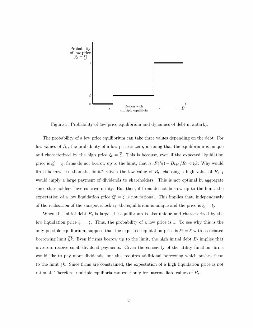
Figure 5: Probability of low price equilibrium and dynamics of debt in autarky.

The probability of a low price equilibrium can take three values depending on the

debt. For low values of Bt, the probability of a low price is zero, meaning that the

equilibrium is unique and characterized by the high price ξt = ξ. This is because, even

if the expected liquidation price is ξet = ξ, firms do not borrow up to the limit, that is,

F (ht) + Bt+1/Rt < ξk. Why would firms borrow less than the limit? Given the low

value of Bt, choosing a high value of Bt+1 would imply a large payment of dividends to

28

Figure 5: Probability of low price equilibrium and dynamics of debt in autarky.

The probability of a low price equilibrium can take three values depending on the debt. For

low values of Bt, the probability of a low price is zero, meaning that the equilibrium is unique

and characterized by the high price ξt = ξ. This is because, even if the expected liquidation

price is ξet = ξ, firms do not borrow up to the limit, that is, F (ht) +Bt+1/Rt < ξk. Why would

firms borrow less than the limit? Given the low value of Bt, choosing a high value of Bt+1

would imply a large payment of dividends to shareholders. This is not optimal in aggregate

since shareholders have concave utility. But then, if firms do not borrow up to the limit, the

expectation of a low liquidation price ξet = ξ is not rational. This implies that, independently

of the realization of the sunspot shock εt, the equilibrium is unique and the price is ξt = ξ.

When the initial debt Bt is large, the equilibrium is also unique and characterized by the

low liquidation price ξt = ξ. Thus, the probability of a low price is 1. To see why this is the

only possible equilibrium, suppose that the expected liquidation price is ξet = ξ with associated

borrowing limit ξk. Even if firms borrow up to the limit, the high initial debt Bt implies that

investors receive small dividend payments. Given the concavity of the utility function, firms

would like to pay more dividends, but this requires additional borrowing which pushes them

to the limit ξk. Since firms are constrained, the expectation of a high liquidation price is not

rational. Therefore, multiple equilibria can exist only for intermediate values of Bt.

24

Next we describe why, starting from the two extreme regions where the equilibrium is unique,

the economy will move to the intermediate region with multiple equilibria. If we start with a low

value of Bt and the borrowing limit is not currently binding, firms have an incentive to increase

the stock of debt over time because the discount factor of investors is smaller than the discount

factor of workers, that is, β < δ. Eventually, they will reach the region with multiple equilibria.

On the other hand, if Bt is initially very high and firms are constrained, their input of labor will

be inefficiently low. Thus, even if the higher discounting of investors creates an incentive for

firms to borrow more, this is counterbalanced by the fact that higher debt must be associated

to lower labor (remember that the enforcement constraint is F (ht) + Bt+1/Rt = ξk). Because

of this, firms will reduce their debt and move to the region with multiple equilibria.14

B Financial Integration

We will show below that multiple equilibria are also possible when countries are financially

integrated. Therefore, sunspot shocks continue to play a role in selecting one of the equilibria in

the multiplicity region. It becomes then important whether each country draws its own sunspot

shock or there is a single draw of a global sunspot shock. We opt for the first case, as made

precise by the following assumption.

Assumption 3. Each country draws its own sunspot shock independently from each other.

The assumption imposes that domestic and foreign draws of sunspot shocks, εt and ε∗t , are

not correlated across countries. Although in a very stylized fashion, this captures the idea

that coordination becomes more difficult when the number of agents increases (an integrated

economy is essentially an economy with a larger number of agents). Essentially, we generate

this by assuming that agents are not perfectly coordinated across borders. As we will see,

this assumption plays an important role for the characterization of equilibria with financially

integrated countries.

A central property of the model with financial integration is that the liquidation prices ξt

and ξ∗t are equalized across countries. This is stated formally in the following lemma.

14Notice that firms are atomistic and, therefore, recognize that multiplicity depends on the aggregate debt Bt,

not their individual debt bt. This also implies that the expected price of liquidated capital and the price of debt

is pinned down regardless of the action of an individual firm. The dependence of sunspot equilibria from the

aggregate stock of debt is also a feature of the model studied in Cole and Kehoe (2000).

25

Lemma 2. With integrated financial markets ξt = ξ∗t .

Proof. Suppose that the equilibrium is characterized by ξt = ξ and ξ∗t = ξ. To have ξt = ξ we

need µt > 0, and to have ξ∗t = ξ we need µ∗t = 0. However, in Section II C we have shown that

with integrated financial markets, µt = µ∗t . Using the same argument, we can exclude equilibria

with ξt = ξ and ξ∗t = ξ.

Hence, financial integration implies perfect cross-country co-movement in the liquidation

prices ξt and ξ∗t . This in turn implies co-movement in financial flows across countries.

The definition of equilibria is similar to the definition provided for the autarky regime with

some small adjustments. In particular, the aggregate states are st = (Wt, εt, ε∗t ) and individual

policies are now functions of the expected prices in both countries, that is, ξet and ξet∗. For exam-

ple, the borrowing policy of domestic firms is denoted by b(st; bt, ξet , ξ

et∗). Even if in equilibrium

the liquidation prices are equalized across countries, this notation allows us to consider out of

equilibrium prices and verify what type of expectations induce binding borrowing constraints.

When countries are integrated, it is as if there is only a representative firm that produces and

borrows in both countries. This ‘globalized’ firm faces the consolidated borrowing constraint

(17) ξtk + ξ∗t k ≥ F (ht) + F (h∗t ) +bt+1 + b∗t+1

Rt.

The left-hand side is the sum of the borrowing limits faced by the globalized firm in each of

the two countries. The right-hand side is the total debt given by the intraperiod loan used to

finance production in both countries plus the intertemporal debt. The globalized firm does not

care in which country it borrows. It only cares about the total debt bt+1 + b∗t+1.

Since ξt = ξ∗t and changes in these prices are the only source of stochastic fluctuations,

we might conclude that financial integration does not change the equilibrium property of the

economy. This conclusion, however, is incorrect. Because Assumption 3 imposes that sunspot

shocks are uncorrelated across borders, even if liquidation prices are equalized across countries,

the probability distribution of ξt = ξ∗t changes when financial markets are integrated.

Assumption 3 is crucial here: countries continue to draw their own sunspot shock indepen-

dently from each other: εt in the domestic country and ε∗t in the foreign country. Therefore,

there are four combinations of realizations of εt and ε∗t . This implies that the probability of a

crisis depends on what combinations of εt and ε∗t can induce a low liquidation price ξt = ξ∗t = ξ.

26

For example, if a low price equilibrium is possible only if both countries draw a low sunspot

shock, that is, εt = ε∗t = 0, then the probability of a crisis is p2. In the autarky regime, in-

stead, this probability is p (provided that multiple equilibria are also possible) because only

the realization of their own sunspot variable matters when financial markets are not integrated.

Alternatively, in the regime with capital mobility we could be in a state in which a negative

draw of the sunspot variable in only one of the two countries is sufficient to induce a low price

equilibrium. In this case the probability of a crisis is p+2(1− p) while the probability in autarky

remains p (again, provided that multiple equilibria are also possible).

Proposition 3. Let εt and ε∗t be two independent random variables that take the value of 0

with probability p ∈ (0, 1) and 1 with probability 1 − p in each of the two countries. If ξ − ξ is

sufficiently large, there exist BA < BA

and BM < B < BM

such that

• In autarky, multiple equilibria exist if and only if Bt ∈ [BA, BA

). In this region, the

probability of a low price equilibrium is p.

• With mobility, multiple equilibria exist if and only if Bt ∈ [BM , BM

). In this region, the

probability of a low price equilibrium is p2 for Bt ∈ [BM , B) and 2p− p2 for Bt ∈ [B, BM

).

• Let fA(Bt) and fM (Bt) be the functions that return Bt+1/Rt in autarky and mobility

when the liquidation price is high. A sufficient condition for BM < BA is that fA(BA) <

fM (BA).

Proof. See Appendix D.

The first part of the proposition simply restates Proposition 2. The second part establishes

a similar result for the economy with financial integration. Notice that, with some abuse of

notation, in the regime with capital mobility we have used Bt to denote the per-country aggregate

debt, that is, Bt = Wt/2. When multiple equilibria exist, the probability of a crisis differs

between the two regimes. In particular, while in autarky the probability is p, with mobility

the probability is initially smaller, p2, but then it increases to 2p − p2. The third part of the

proposition establishes that BM < BA. This implies that in the regime with capital mobility,

crises could emerge for smaller values of debt. We established this property under the sufficient

condition that for Bt = BA, unconstrained borrowing is smaller in autarky.15

15Although we cannot prove this condition analytically, we believe that this is a general property and, as we

will see, it is satisfied in the calibrated model. The reason borrowing should be lower in autarky is because, in

the right-hand side neighbor of BA, the probability of a crisis is higher in autarky (p versus p2). Since crises are

costly for firms and the cost increases with the debt, a higher probability should discourage firms from borrowing.

27

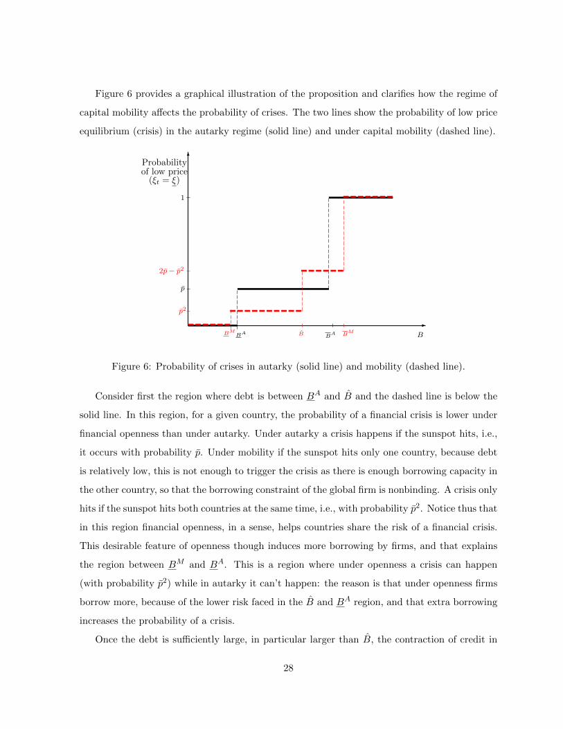
Figure 6 provides a graphical illustration of the proposition and clarifies how the regime of

capital mobility affects the probability of crises. The two lines show the probability of low price

equilibrium (crisis) in the autarky regime (solid line) and under capital mobility (dashed line).

in the regime with capital mobility, crises could emerge for smaller values of debt. We

established this property under the sufficient condition that for Bt = BA, unconstrained

borrowing is smaller in autarky.15

Figure 6 provides a graphical illustration of the proposition and clarifies how the regime

of capital mobility affects the probability of crises. The two lines show the probability of

low price equilibrium (crisis) in the autarky regime (solid line) and under capital mobility

(dashed line).

-

6Probabilityof low price

(ξt = ξ)

1

p

B

p2

2p− p2

BAB

ABMB B

M

Figure 6: Probability of crises in autarky(continuous line) and mobility(dashed line).

Consider first the region where debt is between BA and B and the dashed line is below

the solid line. In this region, for a given country, the probability of a financial crisis is

lower under financial openness than under autarky. Under autarky a crisis happens if the

sunspot hits, i.e. it occurs with probability p. Under mobility if the sunspot hits only one

country, because debt is relatively low, this is not enough to trigger the crisis as there is

15Although we cannot prove this condition analytically, we believe that this is a general property and,

as we will see, it is satisfied in the calibrated model. The reason borrowing should be lower in autarky is

because, in the right-hand-side neighbour of BA, the probability of a crisis is higher in autarky (p versus

p2). Since crisis are costly for firms and the cost increases with the debt, a higher probability should

discourage firms from borrowing.

33

Figure 6: Probability of crises in autarky (solid line) and mobility (dashed line).

Consider first the region where debt is between BA and B and the dashed line is below the

solid line. In this region, for a given country, the probability of a financial crisis is lower under

financial openness than under autarky. Under autarky a crisis happens if the sunspot hits, i.e.,

it occurs with probability p. Under mobility if the sunspot hits only one country, because debt

is relatively low, this is not enough to trigger the crisis as there is enough borrowing capacity in

the other country, so that the borrowing constraint of the global firm is nonbinding. A crisis only

hits if the sunspot hits both countries at the same time, i.e., with probability p2. Notice thus that

in this region financial openness, in a sense, helps countries share the risk of a financial crisis.

This desirable feature of openness though induces more borrowing by firms, and that explains

the region between BM and BA. This is a region where under openness a crisis can happen

(with probability p2) while in autarky it can’t happen: the reason is that under openness firms

borrow more, because of the lower risk faced in the B and BA region, and that extra borrowing

increases the probability of a crisis.

Once the debt is sufficiently large, in particular larger than B, the contraction of credit in

28

only one country is sufficient to make the globalized firm constrained. In this case a crisis arises

when both countries draw a low realization of the sunspot shock, and also when εt = 0 and

ε∗t = 1 or vice versa. Thus, the probability of a crisis becomes p2 + 2p(1− p) = 2p− p2. This is

bigger than the probability in autarky p. In this region openness does not provide risk sharing

but, in a sense, opens the door to the possibility of financial contagion, as a sunspot in just one

country is enough to trigger a global financial crisis.

This figure suggests that the relation between financial openness and vulnerability to financial

crisis is complex. For certain value of debt, openness reduces the risk of financial crisis while for

other values it increases it. So the overall effect of financial openness will depend crucially on

the decisions of agents, i.e., on what is the ergodic set of equilibrium debt. This set is hard to

evaluate analytically, but we will characterize it numerically in Section IV B.

C Discussion

Before moving to the quantitative evaluation of our model we offer a brief discussion of the key

assumptions made so far.

For analytical simplicity we focused on the financial decisions of nonfinancial firms. However,

the mechanism analyzed in the paper can also be thought as operating in other sectors of the

economy, specifically, financial intermediation and household sectors. In the case of banks, we

can think of ξt as the liquidation price for their financial investments. When the banking sector is

illiquid, the liquidation value of the banks’ assets falls, making the whole banking sector illiquid.

In the case of households, we can think of ξt as the liquidation price of houses. When this price

is low, households are financially constrained and this makes the market for houses illiquid. This

could generate a macroeconomic crisis through the collapse in real estate investments. We have

chosen not to formalize explicitly these additional mechanisms in order to keep the model simple.

However, we would like to think of our model as being more general than simply capturing the

changing financial conditions in the nonfinancial corporate sector. As we will see, this view will

be in part reflected in the quantitative section of the paper when we calibrate the model.

An important channel in our model makes a crisis global is that in the equilibrium with

financial integration, the ownership of firms is perfectly diversified across countries. Although in

the data equity ownership remains somewhat home-biased, the bias has declined substantially

29

during the last 15 years as firms became more globalized and institutional investors expanded

their ownership of foreign securities. Therefore, we believe that the mechanism proposed in the

paper, although stylized, is important for understanding the global feature of the 2008 crisis.

Of course, cross-country equity ownership is not the only mechanism through which financial

integration could make a crisis global. Firms, banks and households could hold other types of

foreign securities besides equity. For example, German banks may have purchased collateralized

debt securities issued in the United States before the 2008 crisis. So when the housing market

in the United States contracted, the value of these securities declined, endangering the financial

health of these banks. In this way, a shock that originated in the United States could have

propagated to other countries even if investors in the United States did not own any equity of

German banks. However, we would like to point out that, from an economic point of view—that

is, in terms of investment risk—the ownership of these securities has similar implications to

equity ownership. In other words, the financial condition of German banks may worsen either

because shareholders demand more dividends or because the US investment has fallen in value.

Therefore, we do not consider our transmission mechanism alternative to the mechanism based

on the ownership of foreign collateral assets but just one way of formalizing similar financial

linkages across countries.

IV Quantitative Analysis

In order to bring the theory to the data, we extend the model in two directions: (i) we add

productivity shocks and relax the assumption that the input of capital is fixed; (ii) we allow for

costly adjustment of labor and endogenous utilization.

Productivity Shocks and Capital Accumulation. Capital accumulation introduces ad-

ditional state variables that increase the computational complexity of the model. Since the

enforcement constraint is only occasionally binding, the model must be solved using global ap-

proximation techniques. These techniques become quickly impractical when there is a large

number of state variables. To contain the computational complexity, we assume that the pro-

duction function is linear in the number of workers and the per-worker production takes the

30

form

yt = ztK1−θt kθt l

νt ,

where yt is per-worker output, zt is total factor productivity (TFP), Kt is the worldwide per-

worker capital, kt is the individual per-worker capital and lt is the per-worker effective input of

labor. The aggregate production function is simply ztK1−θt kθt l

νtNt, where Nt is the number of

workers. The effectiveness of labor will be explained below. It is further assumed that θ+ ν < 1

and TFP follows a first order Markov process.

The two countries have the same population of workers and investors and we normalize the

population of workers to 1. Therefore, Kt = (Kt + K∗t )/2. Differences in population will be

taken into account in the calibration.

The dependence of the production function from the worldwide per-worker stock of capital,

Kt, introduces an externality. The purpose of the externality is to have constant returns in

reproducible factors (AK technology) without losing the competitive structure of the model.

The stock of capital evolves according to

kt+1 = (1− τ)kt + Υ

(itkt

)kt,

where it is investment, τ is the rate of depreciation, and the function Υ(.) is strictly increas-

ing and concave, capturing adjustment costs in investment. Adjustment costs are standard in

international macro models as they avoid excessive reallocation of capital across countries.

The enforcement constraint is

xt +bt+1

Rt≤ ξtkt+1,

which differs from equation (3) in that the stock of capital is not fixed but it is chosen endoge-

nously by the firm. In case of default kt+1 will be sold to intermediaries at price ξt as in the

model without capital accumulation.

Endogenous Utilization of Labor. The effective input of labor lt results from the combi-

nation of (measured) hours, ht, and (unmeasured) utilization or effort, et, according to

lt = A(ht, et) ≡[h%−1%

t + e%−1%

t

] %%−1

.

The parameter % is the elasticity of substitution between working hours and actual utilization.

31

Labor utilization is costly because it generates disutility for workers. More specifically,

we assume that the utility function of workers takes the same form as in the previous model.

However, the argument of the utility function is the sum of (measured) hours worked, ht, and

(unmeasured) utilization, et, that is,

U(ct, ht + et) = ln(ct)− α(ht + et)

1+ 1η

1 + 1η

.

With this specification, the marginal utilization cost of labor for the firm is wt and the total

cost of labor is (ht + et)wt.

So far, the addition of labor utilization is inconsequential for the properties of the model.

Since the wage rate is the price for both ht and et, the CES aggregation implies that firms

always choose et = ht. Thus, we can simply focus on ht as we did in the previous model. This

no longer holds if firms face some rigidities in the choice of working hours ht. We formalize this

idea by assuming that firms incur the convex cost

κ(ht − h)2wt,

where h is an exogenous target for per-worker hours.16 This cost makes hours worked ht less

flexible than utilization et. As we will see, this feature allows the model to better capture the

dynamics of the labor wedge.

Normalization. We can now take advantage of the AK structure of the model and normalize

the growing variables by the worldwide per-worker capital Kt. Using the tilde sign to denote

normalized variables—for example, bt = bt/Kt—we rewrite the budget constraint, the law of

motion for capital, and the enforcement constraint for a domestic firm as

bt + dt + it = ztkθt lνt − wt(ht + et)− κ(ht − h)2wt +

gtbt+1

Rt,(18)

gtkt+1 = (1− τ)kt + Υ

(it

kt

)kt,(19)

ξtgtkt+1 ≥ ztkθt lνt +gtbt+1

Rt,(20)

16The cost is multiplied by the wage so that it grows with the economy. Ideally, we would like to use a more

standard adjustment cost, such as κ(ht − ht−1)2wt. This alternative formulation, however, would introduce an

additional state variable, ht−1, which increases the computational complexity of the model.

32

where gt = Kt+1/Kt is the gross growth rate of worldwide per-worker capital. For a foreign firm

we would have the same constraints with asterisks on country-specific variables.

As in the model without capital accumulation, investors hold an internationally diversified

portfolio of shares, and firms use the common discount factor. With a CRRA utility function

for investors, the discount factor takes the form mt+1 = β[(Dt+1 +D∗t+1)/(Dt +D∗t )]−σ, where

σ is the risk aversion parameter. In normalized form, it can be rewritten as

mt+1 = g−σt β

(Dt+1 + D∗t+1

Dt + D∗t

)−σ= g−σt mt+1,

and the optimization problem solved by a domestic firm becomes

V (st; kt, bt) = maxdt,ht,et ,it,bt+1

dt + g1−σt Emt+1V (st+1; kt+1, bt+1)

(21)

subject to (18), (19), (20).

The function Vt = Vt/Kt is the normalized firm’s value and s the normalized aggregate states.

We can now see the analytical convenience of the AK structure: by rescaling the problem

of the firm by K, we do not need to keep track of the worldwide stock of capital. Then,

to characterize the equilibrium, we only need to keep track of two endogenous states: the

normalized worldwide per-capita wealth of workers, Wt = (Bt + B∗t )/2, and the normalized per-

worker capital of domestic firms Kt = Kt/Kt. This is stated formally in the next proposition.

Proposition 4. Denote by Wt = (Bt + B∗t )/2 the normalized worldwide per-capita wealth of

workers and by Kt = Kt/Kt the normalized per-worker capital of domestic firms. The sufficient

state variables for the characterization of the recursive equilibrium are st = (Wt, Kt, zt, z∗t , εt, ε

∗t ).

Proof. The online appendix derives the (normalized) first order conditions and shows that K

does not enter any of these conditions. This follows from the linearity of the production function

and the homogeneity of degree 1 of the adjustment cost function Υ(.). Therefore, the normalized

policies are independent of the worldwide capital. However, the location of worldwide capital

(captured by Kt) still matters because capital cannot be freely reallocated (due to the capital

adjustment cost) in response to country-specific productivity shocks. Keeping track of the per-

capita wealth of workers in each country is not necessary because of consumption risk-sharing

among workers. Only the worldwide wealth of workers, which corresponds to the worldwide debt

of firms, matters. Also, we do not need to keep track of the allocation of debt between home

and foreign firms because, differently from physical capital, there are not adjustment costs in

changing the stock of debt.

33

The property that the Lagrange multipliers and the efficiency wedge 1/(1−µt) are equalized

across countries also applies to this extended version of the model. Therefore, if the enforcement

constraint is binding in one country, it will also be binding in the other country. The definition

of equilibria with endogenous ξt and ξ∗t and the existence of sunspot equilibria are similar to

the version of the model without capital accumulation. The online appendix lists the conditions

that define a dynamic equilibrium and describes the computational procedure. This concludes

the description of the most general version of our model. In the reminder of the paper we first

describe the calibration procedure and then proceed to analyze its quantitative properties.

A Calibration

We interpret country 1 as representative of the United States and country 2 as representative

of the other G7 countries (Canada, France, Germany, Italy, Japan, and the United Kingdom).

Since data for working hours for all G7 countries is only available at an annual frequency, we

calibrate the model yearly.

Following the tradition in business cycle studies, the business sector is interpreted broadly:

firms are the producers of all goods and services used for consumption and investment, including

housing services. This implies that the stock of capital should also be interpreted broadly.

Similarly, the debt in the model should be interpreted as representing total private debt in the

nonfinancial sector, which includes the debt held by both businesses and households. By doing

so, the model can be thought as also capturing the dynamics of some macroeconomic variables

that are more specific to the household sector such as real estate investments. Of course, even

with this broader interpretation, the model does not capture all the financial mechanisms that

could have played a role in the macroeconomic collapse of 2008-2009. Nevertheless, the model

should not be interpreted as only capturing the financial channel in the corporate sector.

We start with the calibration of the model without labor rigidities and set κ = 0. This implies

that the endogenous utilization of labor does not play a significant role since firms always choose

et/ht = 1. The calibration of A(ht, et) will be described when we introduce labor rigidities.

The discount factor for investors, β, and the discount factor for workers, δ, are set to target

an average return on equity of 7 percent and an average interest rate of 3.7 percent. While the

target for the return on equity is standard, the target for the interest rate is greater than the

34

real return on government bonds. However, what matters in the model is the interest rate that

private borrowers pay, which is significantly higher than the real return on government bonds.

We then use the prime rate charged by banks on short-term loans to business from the Federal

Reserve Board database. Net of CPI inflation, the average real rate over the period 1995-2012 is

3.7 percent. Given that we are interpreting the capital stock broadly, we are implicitly assuming

that the return on equity and the interest rate for the nonbusiness sector are the same as in the

business sector (from which we derived the calibration targets). Because of risk, the average

return on equity and the average interest rate are different from the intertemporal discount

rates. Therefore, to pin down β and δ we need an iterative procedure: after setting all other

parameters, we guess the values of β and δ, check the average returns on equity and bonds

calculated in the simulated data, and then we update these two parameters.

The utilities of investors and workers take the logarithmic form, that is, u(ct) = ln(ct) and

U(ct, ht + et) = ln(ct) − α(ht + et)1+1/η/(1 + 1/η). The parameter η determines the Frisch

elasticity of labor supply which we set to 1, a value that is commonly used in macroeconomic

studies. The parameter α is set to target an average working hours of 0.3. The mass of investors

is ω = 0.25. Since the mass of workers is 1, this implies that the relative mass of investors is 20

percent.

The production function has two parameters, ν and θ, which we calibrate by imposing two

targets: an average labor income share of about 0.7 and a return to scale at the firm level of

0.9. The labor income share in the model is equal to ν(1 − µt), which is not constant since

the multiplier µt is positive when the enforcement constraint is binding. However, since in the

calibrated model the constraint is binding only occasionally, the average labor share is not very

different from ν. Therefore, we set ν = 0.7. The return to scale is determined by θ + ν, which

we set to 0.9. This allows us to pin down θ = 0.2. If we interpret the return to scale as deriving

from monopolistic competition, a return to scale of 0.9 implies a price mark-up of about 11

percent, which is close to typical calibrations of macro models with monopolistic competition.

Capital evolves according to kt+1 = (1− τ)kt+ Υ(it/kt)kt with the function Υ(.) specified as

Υ

(itkt

)=

φ11− ζ

(itkt

)1−ζ+ φ2.

This functional form is widely used in the literature (for example, in Jermann 1998). The

35

parameters φ1 and φ2 are chosen so that in the deterministic steady state Tobin’s q is equal to

1 (Qt = 1) and investment is equal to the depreciation of capital (It = τKt). The depreciation

rate is set to τ = 0.06 and the curvature parameter ζ is chosen so that investment is about 3

times more volatile than output. The parameter is chosen through an iterative procedure where

we guess the value of ζ and check whether the investment volatility generated by the model

matches the empirical volatility.

A further modification made for calibration purposes is to assume that the intraperiod loan

is only a fraction ψ of the cash-mismatch xt = wtht + dt + bt− bt+1/Rt. Since we are calibrating

the model annually, the assumption that working capital is equal to the annual production of

the firm is probably excessive. Therefore, we assume that the intraperiod loan is ψxt. This

changes the enforcement constraint to ψxt + bt+1

Rt≤ ξtkt+1 but it does not change in any ways

the qualitative properties of the model. We set ψ = 0.2 which is close to the value used by

Bianchi and Mendoza (2013).

At this point, we are left with the parameters directly related to the stochastic properties

of the shocks. We start with the sunspot shock. We need to calibrate the liquidation prices

ξ and ξ and the probability p (likelihood of drawing the sunspot variable ε = 0). As long as

the distance between the low and high liquidation prices is not too small, the value of ξ is not

important. This is because firms will never borrow up to this limit (again, provided that ξ is

not too close to ξ). The calibration of the lower bound is based on a particular interpretation

of the recent crisis. We think of the recent crisis as characterized by binding constraints. We

can then use the enforcement constraint in 2009 satisfied with the equality sign to calibrate ξ.

More specifically, we use the condition

(22) ξKG72010 = 0.2 Y G7

2009 +BG7

2010

R2009,

where KG72010, Y

G72009, and BG7

2010/R2009 are, respectively, capital, output and private debt for

the aggregation of the G7 countries. Notice that we use 2009 instead of 2008 because the

model is calibrated annually and the crisis started in the last quarter of 2008 and the effects

fully materialized in 2009. A detailed description of the data and how we aggregate national

quantities are provided in Appendix E. Given measurements for the three aggregate variables

(see Appendix E), the value of ξ is found by solving equation (22). The resulting value is

36

ξ = 0.738. If we interpret the intermediation cost as deriving from matching frictions (see

footnote 13), then the probability that an intermediary meets a buyer in the bad equilibrium is

0.738.

The probability of a low realization of the sunspot variable is set to p = 0.04. Thus, a crisis

is a low probability event that on average arises every 25 years. Admittedly, because of the low

frequency of crises, especially in advanced economies, it is difficult to find the precise calibration

target from the data. For this reason we will conduct a sensitivity analysis presented in the

online appendix. Also for the calibration of p we need to use an iterative procedure.

For the productivity shocks we follow the Solow residual approach, that is, we use the empir-

ical series for output, capital, working hours and labor utilization to compute the TFP variable

as a residual from the production function. The problem, however, is that labor utilization et is

not observable. To solve this problem we impute the value of et indirectly using the first order

conditions of the firm for the optimal choice of ht and et.

Consider the production function Yt = ztK1−θt kθtA(ht, et)

ν , where Kt is worldwide per-worker

capital and A(ht, et) is the aggregation of hours and utilization that we specified earlier as a

CES function. Combining the first order conditions for the choice of ht and et we obtain

Ah(ht, et)

Ae(ht, et)= 1 + 2κ(ht − h).

This determines et as a function of ht. Therefore, using this condition and the empirical

series for output, capital, and hours we are able to construct productivity series as residuals

from the production function. A more detailed description is provided in Appendix E.

After constructing the sequences of TFP for the United States, zt, and for the aggregate of

the other G7 countries, z∗t , we use these series to estimate the following V AR(1) model log(zt+1)

log(z∗t+1)

=

ρ1 ρ12

ρ21 ρ2

log(zt)

log(z∗t )

+

εt+1

ε∗t+1

.

The estimated parameters are reported in Table 1. We will then approximate the stochastic

process for TFP with a discrete Markov chain where zt and z∗t can each take three values.

37

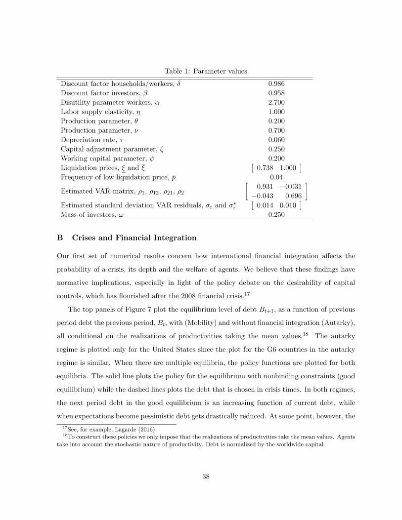
Table 1: Parameter values

Discount factor households/workers, δ 0.986

Discount factor investors, β 0.958

Disutility parameter workers, α 2.700

Labor supply elasticity, η 1.000

Production parameter, θ 0.200

Production parameter, ν 0.700

Depreciation rate, τ 0.060

Capital adjustment parameter, ζ 0.250

Working capital parameter, ψ 0.200

Liquidation prices, ξ and ξ[

0.738 1.000]

Frequency of low liquidation price, p 0.04

Estimated VAR matrix, ρ1, ρ12, ρ21, ρ2

[0.931 −0.031

−0.043 0.696

]Estimated standard deviation VAR residuals, σε and σ∗ε

[0.014 0.010

]Mass of investors, ω 0.250

B Crises and Financial Integration

Our first set of numerical results concern how international financial integration affects the

probability of a crisis, its depth and the welfare of agents. We believe that these findings have

normative implications, especially in light of the policy debate on the desirability of capital

controls, which has flourished after the 2008 financial crisis.17

The top panels of Figure 7 plot the equilibrium level of debt Bt+1, as a function of previous

period debt the previous period, Bt, with (Mobility) and without financial integration (Autarky),

all conditional on the realizations of productivities taking the mean values.18 The autarky

regime is plotted only for the United States since the plot for the G6 countries in the autarky

regime is similar. When there are multiple equilibria, the policy functions are plotted for both

equilibria. The solid line plots the policy for the equilibrium with nonbinding constraints (good

equilibrium) while the dashed lines plots the debt that is chosen in crisis times. In both regimes,

the next period debt in the good equilibrium is an increasing function of current debt, while

when expectations become pessimistic debt gets drastically reduced. At some point, however, the

17See, for example, Lagarde (2016).18To construct these policies we only impose that the realizations of productivities take the mean values. Agents

take into account the stochastic nature of productivity. Debt is normalized by the worldwide capital.

38

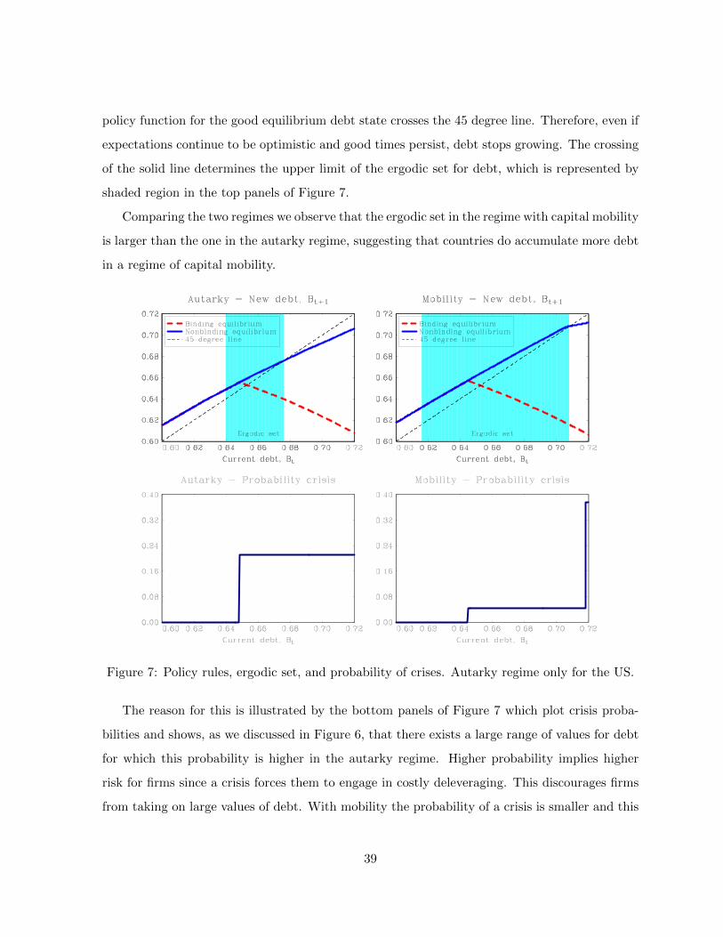
policy function for the good equilibrium debt state crosses the 45 degree line. Therefore, even if

expectations continue to be optimistic and good times persist, debt stops growing. The crossing

of the solid line determines the upper limit of the ergodic set for debt, which is represented by

shaded region in the top panels of Figure 7.

Comparing the two regimes we observe that the ergodic set in the regime with capital mobility

is larger than the one in the autarky regime, suggesting that countries do accumulate more debt

in a regime of capital mobility.

Figure 7: Policy rules, ergodic set, and probability of crises. Autarky regime only for the US.

The reason for this is illustrated by the bottom panels of Figure 7 which plot crisis proba-

bilities and shows, as we discussed in Figure 6, that there exists a large range of values for debt

for which this probability is higher in the autarky regime. Higher probability implies higher

risk for firms since a crisis forces them to engage in costly deleveraging. This discourages firms

from taking on large values of debt. With mobility the probability of a crisis is smaller and this

39

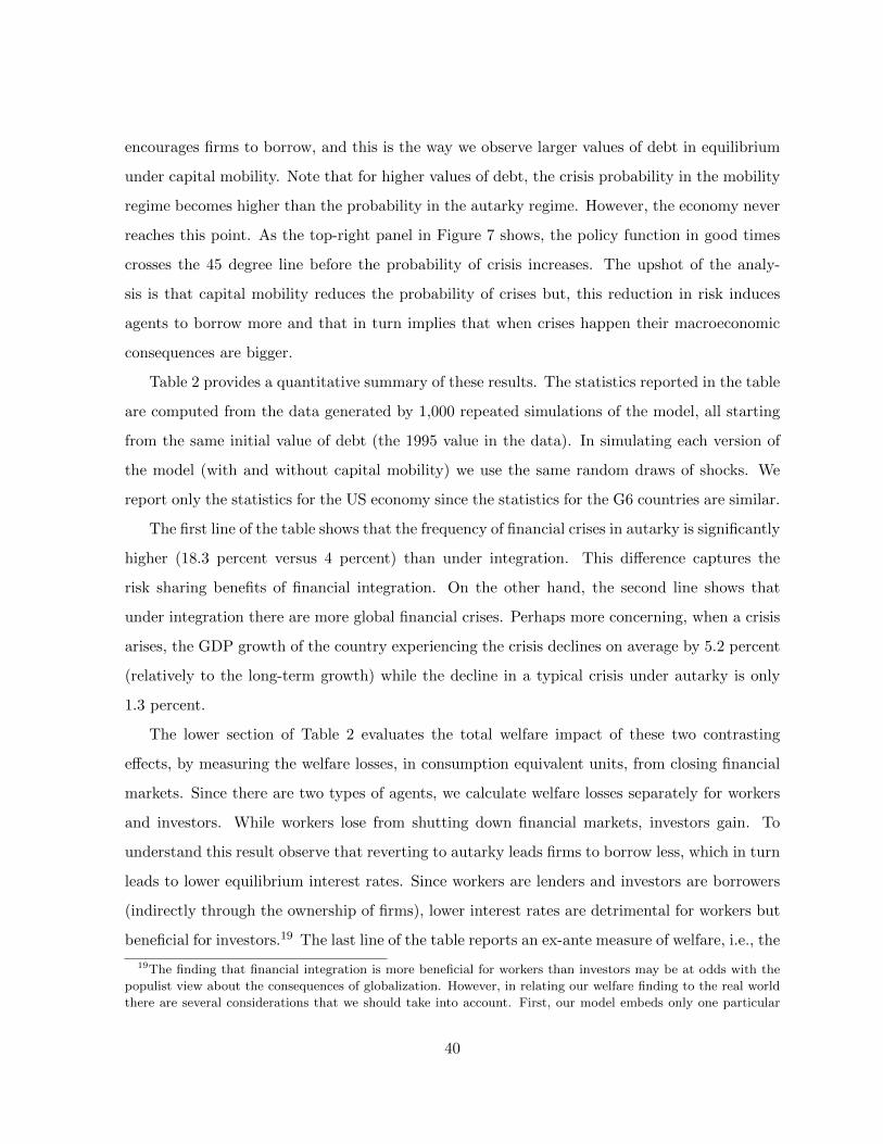
encourages firms to borrow, and this is the way we observe larger values of debt in equilibrium

under capital mobility. Note that for higher values of debt, the crisis probability in the mobility

regime becomes higher than the probability in the autarky regime. However, the economy never

reaches this point. As the top-right panel in Figure 7 shows, the policy function in good times

crosses the 45 degree line before the probability of crisis increases. The upshot of the analy-

sis is that capital mobility reduces the probability of crises but, this reduction in risk induces

agents to borrow more and that in turn implies that when crises happen their macroeconomic

consequences are bigger.

Table 2 provides a quantitative summary of these results. The statistics reported in the table

are computed from the data generated by 1,000 repeated simulations of the model, all starting

from the same initial value of debt (the 1995 value in the data). In simulating each version of

the model (with and without capital mobility) we use the same random draws of shocks. We

report only the statistics for the US economy since the statistics for the G6 countries are similar.

The first line of the table shows that the frequency of financial crises in autarky is significantly

higher (18.3 percent versus 4 percent) than under integration. This difference captures the

risk sharing benefits of financial integration. On the other hand, the second line shows that

under integration there are more global financial crises. Perhaps more concerning, when a crisis

arises, the GDP growth of the country experiencing the crisis declines on average by 5.2 percent

(relatively to the long-term growth) while the decline in a typical crisis under autarky is only

1.3 percent.

The lower section of Table 2 evaluates the total welfare impact of these two contrasting

effects, by measuring the welfare losses, in consumption equivalent units, from closing financial

markets. Since there are two types of agents, we calculate welfare losses separately for workers

and investors. While workers lose from shutting down financial markets, investors gain. To

understand this result observe that reverting to autarky leads firms to borrow less, which in turn

leads to lower equilibrium interest rates. Since workers are lenders and investors are borrowers

(indirectly through the ownership of firms), lower interest rates are detrimental for workers but

beneficial for investors.19 The last line of the table reports an ex-ante measure of welfare, i.e., the

19The finding that financial integration is more beneficial for workers than investors may be at odds with the

populist view about the consequences of globalization. However, in relating our welfare finding to the real world

there are several considerations that we should take into account. First, our model embeds only one particular

40

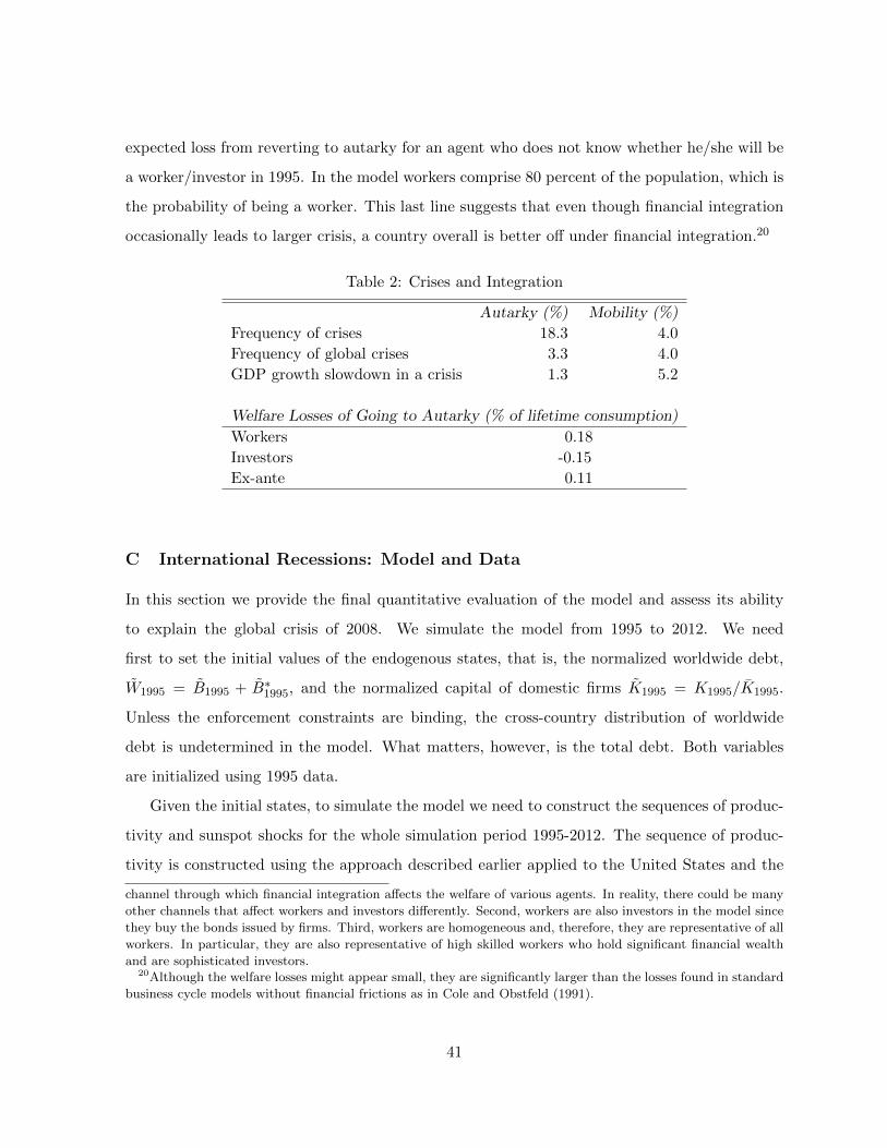
expected loss from reverting to autarky for an agent who does not know whether he/she will be

a worker/investor in 1995. In the model workers comprise 80 percent of the population, which is

the probability of being a worker. This last line suggests that even though financial integration

occasionally leads to larger crisis, a country overall is better off under financial integration.20

Table 2: Crises and Integration

Autarky (%) Mobility (%)

Frequency of crises 18.3 4.0

Frequency of global crises 3.3 4.0

GDP growth slowdown in a crisis 1.3 5.2

Welfare Losses of Going to Autarky (% of lifetime consumption)

Workers 0.18

Investors -0.15

Ex-ante 0.11

C International Recessions: Model and Data

In this section we provide the final quantitative evaluation of the model and assess its ability

to explain the global crisis of 2008. We simulate the model from 1995 to 2012. We need

first to set the initial values of the endogenous states, that is, the normalized worldwide debt,

W1995 = B1995 + B∗1995, and the normalized capital of domestic firms K1995 = K1995/K1995.

Unless the enforcement constraints are binding, the cross-country distribution of worldwide

debt is undetermined in the model. What matters, however, is the total debt. Both variables

are initialized using 1995 data.

Given the initial states, to simulate the model we need to construct the sequences of produc-

tivity and sunspot shocks for the whole simulation period 1995-2012. The sequence of produc-

tivity is constructed using the approach described earlier applied to the United States and the

channel through which financial integration affects the welfare of various agents. In reality, there could be many

other channels that affect workers and investors differently. Second, workers are also investors in the model since

they buy the bonds issued by firms. Third, workers are homogeneous and, therefore, they are representative of all

workers. In particular, they are also representative of high skilled workers who hold significant financial wealth

and are sophisticated investors.20Although the welfare losses might appear small, they are significantly larger than the losses found in standard

business cycle models without financial frictions as in Cole and Obstfeld (1991).

41

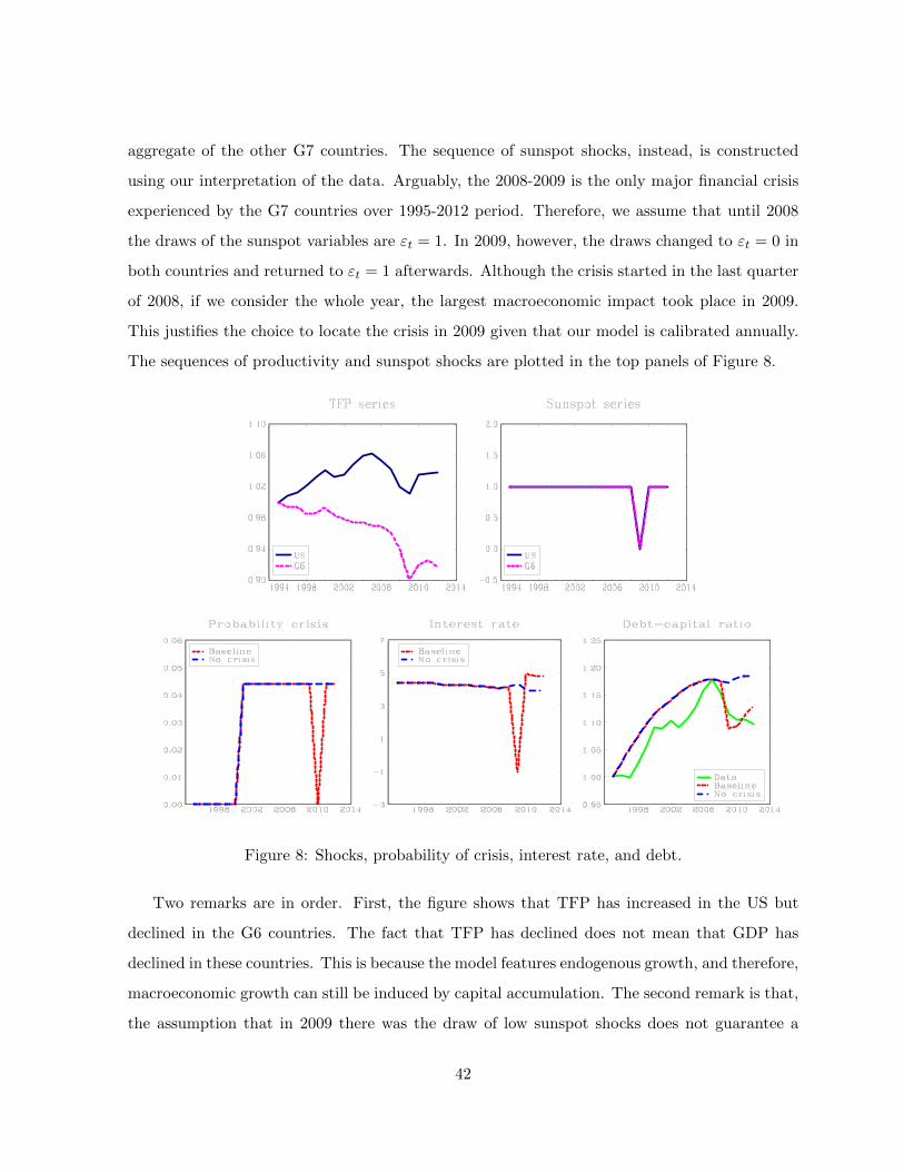
aggregate of the other G7 countries. The sequence of sunspot shocks, instead, is constructed

using our interpretation of the data. Arguably, the 2008-2009 is the only major financial crisis

experienced by the G7 countries over 1995-2012 period. Therefore, we assume that until 2008

the draws of the sunspot variables are εt = 1. In 2009, however, the draws changed to εt = 0 in

both countries and returned to εt = 1 afterwards. Although the crisis started in the last quarter

of 2008, if we consider the whole year, the largest macroeconomic impact took place in 2009.

This justifies the choice to locate the crisis in 2009 given that our model is calibrated annually.

The sequences of productivity and sunspot shocks are plotted in the top panels of Figure 8.

Given the initial states, to simulate the model we need to construct the sequences of produc-

tivity and sunspot shocks for the whole simulation period 1995-2012. The sequence of produc-

tivity is constructed using the approach described earlier applied to the United States and the

aggregate of the other G7 countries. The sequence of sunspot shocks, instead, is constructed

using our interpretation of the data. Arguably, the 2008-2009 is the only major financial crisis

experienced by the G7 countries over 1995-2012 period. Therefore, we assume that until 2008

the draws of the sunspot variables are εt = 1. In 2009, however, the draws changed to εt = 0 in

both countries and returned to εt = 1 afterwards. Although the crisis started in the last quarter

of 2008, if we consider the whole year, the largest macroeconomic impact took place in 2009.

This justifies the choice to locate the crisis in 2009 given that our model is calibrated annually.

The sequences of productivity and sunspot shocks are plotted in the top panels of Figure 8.

Figure 8: Shocks, probability of crisis, interest rate and debt.

Two remarks are in order. First, the figure shows that TFP has increased in the US but

declined in the G6 countries. The fact that the TFP has declined does not mean that GDP

has declined in these countries. This is because the model features endogenous growth, and

therefore, macroeconomic growth can still be induced by capital accumulation.

The second remark is that, the assumption that in 2009 there was the draw of low sunspot

37

Figure 8: Shocks, probability of crisis, interest rate, and debt.

Two remarks are in order. First, the figure shows that TFP has increased in the US but

declined in the G6 countries. The fact that TFP has declined does not mean that GDP has

declined in these countries. This is because the model features endogenous growth, and therefore,

macroeconomic growth can still be induced by capital accumulation. The second remark is that,

the assumption that in 2009 there was the draw of low sunspot shocks does not guarantee a

42

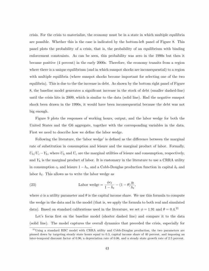
crisis. For the crisis to materialize, the economy must be in a state in which multiple equilibria

are possible. Whether this is the case is indicated by the bottom-left panel of Figure 8. This

panel plots the probability of a crisis, that is, the probability of an equilibrium with binding

enforcement constraints. As can be seen, this probability was zero in the 1990s but then it

became positive (4 percent) in the early 2000s. Therefore, the economy transits from a region

where there is a unique equilibrium (and in which sunspot shocks are inconsequential) to a region

with multiple equilibria (where sunspot shocks become important for selecting one of the two

equilibria). This is due to the the increase in debt. As shown by the bottom right panel of Figure

8, the baseline model generates a significant increase in the stock of debt (smaller dashed-line)

until the crisis hits in 2009, which is similar to the data (solid line). Had the negative sunspot

shock been drawn in the 1990s, it would have been inconsequential because the debt was not

big enough.

Figure 9 plots the responses of working hours, output, and the labor wedge for both the

United States and the G6 aggregate, together with the corresponding variables in the data.

First we need to describe how we define the labor wedge.

Following the literature, the ‘labor wedge’ is defined as the difference between the marginal

rate of substitution in consumption and leisure and the marginal product of labor. Formally,

Uh/Uc−Yh, where Uh and Uc are the marginal utilities of leisure and consumption, respectively,

and Yh is the marginal product of labor. It is customary in the literature to use a CRRA utility

in consumption ct and leisure 1− ht, and a Cobb-Douglas production function in capital kt and

labor ht. This allows as to write the labor wedge as

(23) Labor wedge =φct

1− ht− (1− θ) yt

ht,

where φ is a utility parameter and θ is the capital income share. We use this formula to compute

the wedge in the data and in the model (that is, we apply the formula to both real and simulated

data). Based on standard calibrations used in the literature, we set φ = 1.91 and θ = 0.4.21

Let’s focus first on the baseline model (shorter dashed line) and compare it to the data

(solid line). The model captures the overall dynamics that preceded the crisis, especially for

21Using a standard RBC model with CRRA utility and Cobb-Douglas production, the two parameters are

pinned down by targeting steady state hours equal to 0.3, capital income share of 40 percent, and imposing an

inter-temporal discount factor of 0.96, a depreciation rate of 0.06, and a steady state growth rate of 2.5 percent.

43

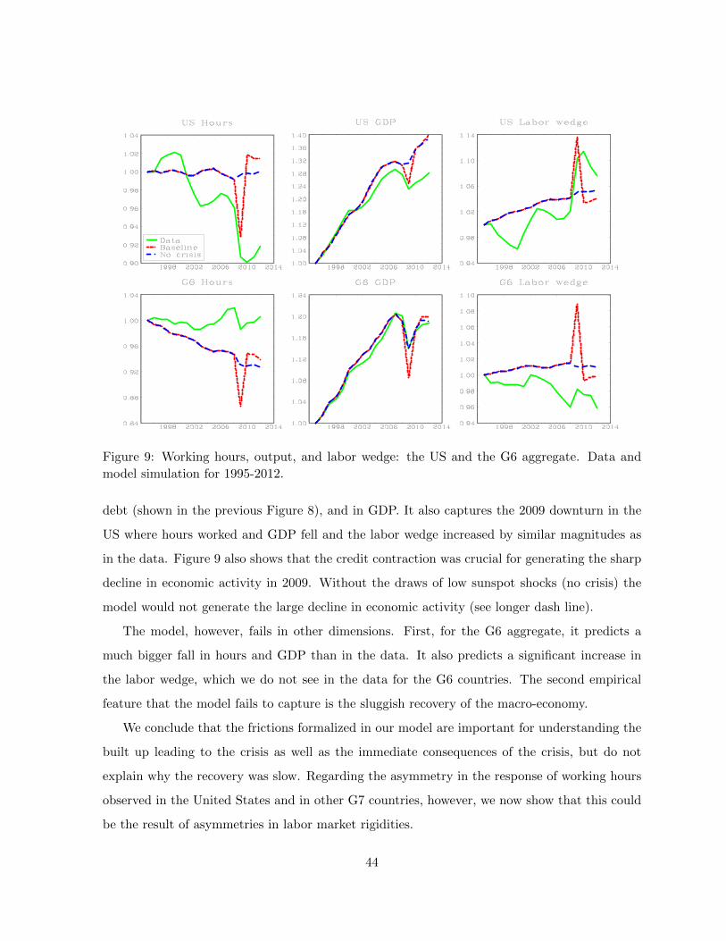
Figure 9: Working hours, output, and labor wedge: the US and the G6 aggregate. Data and

model simulation for 1995-2012.

debt (shown in the previous Figure 8), and in GDP. It also captures the 2009 downturn in the

US where hours worked and GDP fell and the labor wedge increased by similar magnitudes as

in the data. Figure 9 also shows that the credit contraction was crucial for generating the sharp

decline in economic activity in 2009. Without the draws of low sunspot shocks (no crisis) the

model would not generate the large decline in economic activity (see longer dash line).

The model, however, fails in other dimensions. First, for the G6 aggregate, it predicts a

much bigger fall in hours and GDP than in the data. It also predicts a significant increase in

the labor wedge, which we do not see in the data for the G6 countries. The second empirical

feature that the model fails to capture is the sluggish recovery of the macro-economy.

We conclude that the frictions formalized in our model are important for understanding the

built up leading to the crisis as well as the immediate consequences of the crisis, but do not

explain why the recovery was slow. Regarding the asymmetry in the response of working hours

observed in the United States and in other G7 countries, however, we now show that this could

be the result of asymmetries in labor market rigidities.

44

Labor Markets Rigidities. While the baseline model captures relatively well the US cri-

sis, it overpredicts the response of labor and output in the G6 aggregate. It also predicts a

significant increase in the labor wedge of the G6 aggregate which is not present in the data.

The heterogeneous response of hours and labor wedge in the US and other G7 countries is well

known. Ohanian and Raffo (2012) find that, while the US labor wedge dropped dramatically

during the recent crisis, most of the industrialized countries experienced mild declines. At the

same time, while the contraction in GDP was not very different, the contraction in hours was

much stronger in the US. We will now show that the heterogeneous response of labor can be

reconciled, at least in part, with differences in labor market rigidities.

To capture heterogeneous labor market rigidities, we assume that the cost κ(ht − h)2 could

differ between the two countries. We continue to assume that the hiring policy is fully flexible in

the United States (that is, κUS = 0), but it is less so for the G6 aggregate (κG6 > 0). Although in

the baseline model we did not have to calibrate the function A(ht, et) ≡[h%−1%

t + e%−1%

t

] %%−1

, with

labor frictions the calibration of this function becomes important. We choose a relatively high

elasticity of substitution between hours and utilization and set it to % = 5. For the employment

cost we set κG6 = 1 and h to the average value of working hours which we calibrated to 0.3.

The TFP sequence is recalculated using the new parametrization.

Figure 10 compares the simulation of the model with and without hiring frictions. As we

can see, adding labor frictions brings the model much closer to the data for the G6 aggregate,

without changing the predictions for the United States that were already close to the data. In

particular, we now observe that the drop in hours and output in the G6 countries during the

crisis is very similar to the data. What the model does not capture is the increase in G6 hours

before the crisis. Interestingly, now the model does not generate a significant increase in the

labor wedge for the G6 countries. In fact the whole pattern of the labor wedge during the

1995-2012 period is very close to the data.

The stability of the labor wedge during the crisis has a simple intuition. As market conditions

deteriorated in the G6 countries, employers reduced utilization (which remained flexible) rather

than hours (which were costly to change). This generates a significant drop in production but

limited change in hours. For an analyst who looks at the economy through the lens of a standard

real business cycle model with full utilization of labor, this will be interpreted as a large drop

45

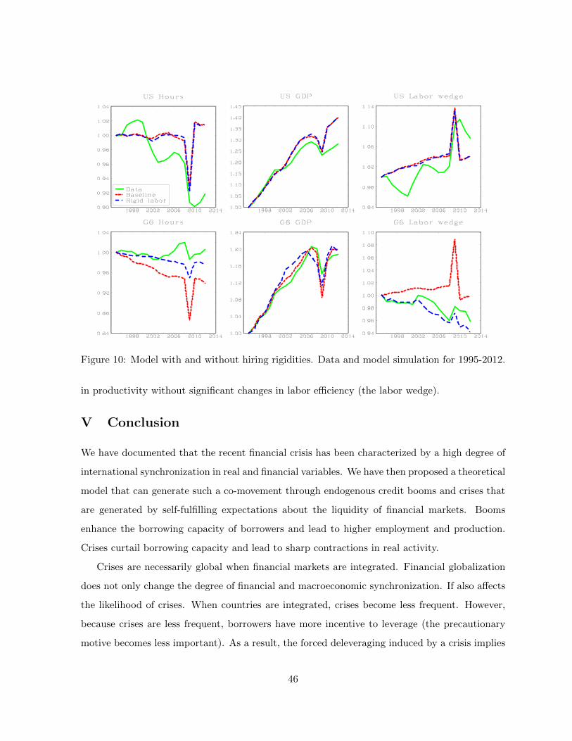
Figure 10: Model with and without hiring rigidities. Data and model simulation for 1995-2012.

in productivity without significant changes in labor efficiency (the labor wedge).

V Conclusion

We have documented that the recent financial crisis has been characterized by a high degree of

international synchronization in real and financial variables. We have then proposed a theoretical

model that can generate such a co-movement through endogenous credit booms and crises that

are generated by self-fulfilling expectations about the liquidity of financial markets. Booms

enhance the borrowing capacity of borrowers and lead to higher employment and production.

Crises curtail borrowing capacity and lead to sharp contractions in real activity.

Crises are necessarily global when financial markets are integrated. Financial globalization

does not only change the degree of financial and macroeconomic synchronization. If also affects

the likelihood of crises. When countries are integrated, crises become less frequent. However,

because crises are less frequent, borrowers have more incentive to leverage (the precautionary

motive becomes less important). As a result, the forced deleveraging induced by a crisis implies

46

larger macroeconomic contractions.

We have explored the quantitative importance of liquidity induced crises by calibrating the

model to the United States and other G7 countries. The simulation over the period 1995-2012

shows that the model captures several features of real and financial data not only during the

crisis but also in the period that preceded the crisis. The setup can also help us understand

a number of macroeconomic features that are hallmarks of financial crises in general and not

specific to the 2008 crisis. An important feature that the model does not capture is the sluggish

recovery observed after the crisis. This suggests that although a liquidity shortage is important

for explaining the initial collapse in economic activity which is typical of a financial crisis, it

cannot explain the sluggish recovery. We think that exploring the potential mechanisms through

which a financial crisis can generate a slow recovery is an important direction for future research.

Although this study focuses on the role of financial factors for generating international co-

movement, it does not exclude the importance of other channels. As far as the recent crisis

is concerned, we do not claim that a credit contraction was the only cause of the crisis. We

have shown, however, that credit market conditions can go a long way in capturing some of

the salient features of the crisis and, especially, its unprecedented international synchronization.

Our findings are also relevant for policy. If crises are driven by global self-fulfilling liquidity

shortages, policies geared toward the provision of liquidity in financial markets could avoid bad

equilibria and have important real effects. Macro-prudential policies similar to those studied in

Bianchi and Mendoza (2013) may also be desirable.

47

References

Arellano, Cristina, Yan Bai, and Patrick J. Kehoe. 2012. “Financial Frictions and Fluctuations

in Volatility.” Federal Reserve Bank of Minneapolis Research Department Staff Report 466.

Bacchetta, Philippe, Kenza Benhima, and Celine Poilly. 2014. “Corporate Cash and Employ-

ment.” Swiss Finance Institute Research Paper No. 14-01.

https://ssrn.com/abstract=2394742.

Bacchetta, Philippe, and Eric van Wincoop. 2016. “The Great Recession: A Self-Fulfilling

Global Panic.” American Economic Journal: Macroeconomics 8 (4): 177-98.

Backus, David K., Patrick J. Kehoe, and Finn E. Kydland. 1992. “International Real Business

Cycles.” Journal of Political Economy 100 (4): 745-75.

Benmelech, Efraim, and Nittai K. Bergman. 2012. “Credit Traps.” American Economic Review

120 (6): 3004-32.

Bentolila, Samuel, Marcel Jansen, Gabriel Jimenez, and Sonia Ruano. 2013. “When Credit

Dries Up: Job Losses in the Great Recession.” IZA Discussion Paper 7807.

Bianchi, Javier. 2011. “Overborrowing and Systemic Externalities in the Business Cycle.” Amer-

ican Economic Review 101 (7): 3400-26.

Bianchi, Javier, and Enrique Mendoza. 2013. “Optimal Time-Consistent Macroprudential

Policy.” NBER Working Paper 19704.

Boissay, Frederic, Fabrice Collard, and Frank Smets. 2013. “Booms and Systemic Banking

Crises.” ECB Working Paper 1514.

Brunnermeier, Markus, and Yuliy Sannikov. 2014. “A Macroeconomic Model with a Financial

Sector.” American Economic Review 104 (2): 379-421.

Cetorelli, Nicola, and Linda S. Goldberg. 2012. “Banking Globalization and Monetary Trans-

mission.” Journal of Finance 67 (5): 1811-43.

48

Chodorow-Reich, Gabriel. 2014. “The Employment Effects of Credit Market Disruptions:

Firm level Evidence from the 2008-9 Financial Crisis.” Quarterly Journal of Economics

129 (1): 1-59.

Christiano, Lawrence J., Roberto Motto, and Massimo Rostagno. 2014. “Risk Shocks.” Amer-

ican Economic Review 104 (1): 27-65.

Claessens, Stijn, Ayhan Kose, and Marco E. Terrones. 2011. “Financial Cycles: What? How?

When?” CEPR Discussion Paper 8379.

Cole, Harold L., and Timothy J. Kehoe. 2000. “Self-Fulfilling Debt Crises.” Review of Eco-

nomic Studies 67 (1): 91-116.

Cole, Harold L., and Maurice Obstfeld. 1991. “Commodity Trade and International Risk

Sharing: How Much Do Financial Markets Matter?” Journal of Monetary Economics 28

(1): 3-24.

Dedola, Luca, and Giovanni Lombardo. 2010. “Financial Frictions, Financial Integration and

the International Propagation of Shocks.” Economic Policy 27 (70): 319-59.

Devereux, Michael B., and Alan Sutherland. 2011. “Evaluating International Financial Inte-

gration under Leverage Constraints.” European Economic Review 55 (3): 427-42.

Devereux, Michael B., and James Yetman. 2010. “Leverage Constraints and the International

Transmission of Shocks.” Journal of Money, Credit and Banking 42 (s1): 71-105.

Diamond, Peter A. 1982. “Aggregate Demand Management in Search Equilibrium.” Journal

of Political Economy 90 (5): 881-94.

Eisfeldt, Andrea L., and Adriano A. Rampini. 2006. “Capital Reallocation and Liquid-

ity.” Journal of Monetary Economics 53 (3): 369-99.

Gao, Pengjie, and Hayong Yun. 2009. “Commercial Paper, Lines of Credit, and the Real

Effects of the Financial Crisis of 2008: Firm-Level Evidence from the Manufacturing In-

dustry.” http://hdl.handle.net/1783.1/72569.

49

Gertler, Mark, and Peter Karadi. 2011. “A Model of Unconventional Monetary Policy.” Journal

of Monetary Economics 58 (1): 17-34.

Goldberg, Jonathan E. 2013. “Credit-Crunch Dynamics with Uninsured Investment Risk.” Fed-

eral Reserve Board Finance and Economics Discussion Series 2013-31.

Goldberg, Linda S., and Charles D. Kolstad. 1995. “Foreign Direct Investment, Exchange Rate

Variability and Demand Uncertainty.” International Economic Review 36 (4): 855-73.

Greenstone, Michael, Alexandre Mas, and Hoai-Luu Nguyen. 2014. “Do Credit Market Shocks

Affect the Real Economy? Quasi-Experimental Evidence from the Great Recession and

Normal Economic Times.” NBER Working Paper 20704.

Guerrieri, Veronica, and Guido Lorenzoni. 2011. “Credit Crises, Precautionary Savings, and

the Liquidity Trap.” NBER Working Paper 17583.

Hart, Oliver, and John Moore. 1994. “A Theory of Debt Based on the Inalienability of Human

Capital.” Quarterly Journal of Economics 109 (4): 841-79.

Imbs, Jean. 2010. “The First Global Recession in Decades.” IMF Economic Review 58 (2):

327-54.

Jermann, Urban J. 1998. “Asset Pricing in Production Economies.” Journal of Monetary

Economics 41 (2): 257-75.

Jermann, Urban, and Vincenzo Quadrini. 2012. “Macroeconomic Effects of Financial Shocks.” Amer-

ican Economic Review 102 (1): 238-71.

Khan, Aubhik, and Julia K. Thomas. 2013. “Credit Shocks and Aggregate Fluctuations in an

Economy with Production Heterogeneity.” Journal of Political Economy 121 (6): 1055-

1107.

Kiyotaki, Nobuhiro, and John Moore. 1997. “Credit Cycles.” Journal of Political Economy

105 (2): 211-48.

50

Kocherlakota, Narayana. 2009. “Bursting Bubbles: Consequences and Cures.” Paper presented

at the Macroeconomic and Policy Challenges Following Financial Meltdowns Conference,

hosted by the International Monetary Fund, Washington, DC.

Kollmann, Robert. 2013. “Global Banks, Financial Shocks, and International Business Cycles:

Evidence from an Estimated Model.” Journal of Money, Credit and Banking 45 (s2):

159-95.

Kollmann, Robert, Zeno Enders, and Gernot J. Muller. 2011. “Global Banking and Interna-

tional Business Cycle.” European Economic Review 55 (3): 407-26.

Lagarde, Christine. 2016. “The Role of Emerging Markets in a New Global Partnership for

Growth.” Speech delivered at the University of Maryland, College Park, MD.

https://www.imf.org/en/News/Articles/2015/09/28/04/53/sp020416.

Liu, Zheng, and Pengfei Wang. 2014. “Credit Constraints and Self-Fulfulling Business Cy-

cles.” American Economic Journal: Macroeconomics 6 (1): 32-69.

Liu, Zheng, Pengfei Wang, and Tao Zha. 2013. “Land-Price Dynamics and Macroeconomic

Fluctuations.” Econometrica 81 (3): 1147-84.

Lucas, Robert E., Jr., and Nancy L. Stokey. 2011. “Liquidity Crises.” Federal Reserve Bank

of Minneapolis Economic Policy Paper 11-3.

Martin, Alberto, and Jaume Ventura. 2012. “Economic Growth with Bubbles.” American

Economic Review 102 (6): 3033-58.

Mendoza, Enrique J. 2010. “Sudden Stops, Financial Crises, and Leverage.” American Eco-

nomic Review 100 (5): 1941-66.

Miao, Jianjun, and Pengfei Wang. 2017. “Asset Bubbles and Credit Constraints.” Unpublished.

Ohanian, Lee E. 2010. “The Economic Crisis from a Neoclassical Perspective.” Journal of

Economic Perspectives 24 (4): 45-66.

51

Ohanian, Lee E., and Andrea Raffo. 2012. “Aggregate Hours Worked in OECD Countries:

New Measurement and Implications for Business Cycles.” Journal of Monetary Economics

59 (1): 40-56.

Reinhart, Carmen M., and Kenneth S. Rogoff. 2009. This Time Is Different: Eight Centuries

of Financial Folly. Princeton, NJ: Princeton University Press.

Schularick, Moritz, and Alan M. Taylor. 2012. “Credit Booms Gone Bust: Monetary Policy,

Leverage Cycles, and Financial Crises, 1870-2008.” American Economic Review 102 (2):

1029-61.

Shleifer, Andrei, and Robert W. Vishny. 1992. “Liquidation Values and Debt Capacity: A

Market Equilibrium Approach.” Journal of Finance 47 (4): 1343-66.

52

Appendix

A Debt Renegotiation

The enforcement constraint is derived from the following assumptions. Default arises at the end of the

period before repaying the intratemporal loan xt = F (ht). In case of default, the firm retains the liquidity

xt and the lender confiscates the physical capital which will be sold at price ξt.

Define the value of the firm recursively as Vt(bt) = dt+Etmt+1Vt+1(bt+1), where mt+1 is the discount

factor, taken as given by an individual firm. Since default takes place at the end of the period, after

paying dividends, the value of not defaulting is Etmt+1Vt+1(bt+1).

In the event of default the parties negotiate a repayment τt. If they reach an agreement, the firm

continues operation and its value is Etmt+1Vt+1(bt+1) + xt − τt. The firm retains its continuation value

Etmt+1Vt+1(bt+1) plus the liquidity xt net of the bargained repayment τt. We are assuming that after

reaching an agrement, the firm pays xt − τt to the shareholders (investors). This is in addition to

the dividends dt paid at the beginning of the period.22 Without an agreement the firm retains only the

divertible liquidity xt (threat value). The value of an agreement is the difference between the renegotiation

value and the threat value, that is,

(A1) Etmt+1Vt+1(bt+1)− τt.

Let’s now consider the lender. With an agreement the lender gets τt + bt+1/Rt. The intertemporal

debt is discounted, since it will be repaid next period. Without an agreement the lender receives the

liquidation value, ξtk (threat value). Thus, the net value from renegotiation is

(A2) τt +bt+1

Rt− ξtk.

The net surplus is the sum of the values for the firm, (A1), and the lender, (A2),

(A3) St(bt+1) = Etmt+1Vt+1(bt+1) +bt+1

Rt− ξtk.

Under the assumption that the firm has all bargaining power, the default value is xt + St(bt+1).

Incentive compatibility requires that the value of not defaulting is (weakly) bigger than the value of

defaulting, that is,

Etmt+1Vt+1(bt+1) ≥ xt + St(bt+1).

Substituting the definition of the net renegotiation surplus St(bt+1) and rearranging, we obtain the

enforcement constraint ξtk = xt + bt+1/Rt.

B First Order Conditions for Problem (4)

Let λt and µt be the Lagrange multipliers for the budget and enforcement constraints. Taking derivatives

with respect to dt, ht and bt+1 we obtain

1− λt = 0

λt

[Fh(ht)− wt

]− µtFh(ht) = 0

Etmt+1Vb(st+1; bt+1) +λtRt− µtRt

= 0.

22We could allow the firm to retain the liquidity xt − τt and invest it in bonds with gross return Rt. The

payment of dividends, however, weakly dominates the investment in bond since RtEtmt+1 ≤ 1 (see equation (7)).

53

Using the envelope condition Vb(st; bt) = −λt to replace the derivative of the value function in the third

equation and eliminating λt using the first equation, we obtain (7) and (8).

C Proof of Proposition 2

Sunspot equilibria arise when, for a given state Bt, two equilibria are possible: the equilibrium with

binding enforcement constraint and low liquidation price ξt = ξ (tight credit) and the equilibrium with

nonbinding enforcement constraint and high liquidation price ξt = ξ (loose credit). When both equilibria

are possible, the actual equilibrium is selected by the random draw of the nonfundamental shock ε ∈ 0, 1.If for a given state Bt only one equilibrium is possible, the random draw of ε ∈ 0, 1 is irrelevant. In

what follows we show that there are B < B for which the ‘loose credit’ equilibrium is unique if Bt < B;

the ‘tight credit’ equilibrium is unique if Bt ≥ B; for B ≤ Bt < B the ‘tight credit’ equilibrium arises

with probability p and the ‘loose credit’ equilibrium with probability 1− p. Furthermore, independently

of the initial state Bt, the debt will reach the multiplicity region. We show this by contradiction.

• Loose credit cannot be a steady state. Suppose that the initial state Bt is such that the

enforcement constraint is not initially binding. Furthermore, suppose that the constraint will not

be binding in all future periods. Therefore, we start with the assumption that the economy remains

in the loose credit equilibrium and the liquidation price is ξt = ξ for all t. Since the liquidation price

remains constant over time, there is no uncertainty and the economy will converge to a steady state.

We now show that in this steady state the enforcement constraint must be binding, contradicting

the assumption that loose credit can persist forever.

From the workers’ first order condition (10) evaluated at the steady state we have δR = 1. From

the firms’ first order condition (7), also evaluated at the steady state, we have βR = 1− µ. Since

δ > β, these two conditions imply that the multiplier associated with the enforcement constraint µ

is strictly positive. Therefore, the enforcement constraint must be binding in a steady state. This

contradicts the assumption that loose credit with ξt = ξ can be a steady state.

• Tight credit cannot be a steady state. If equilibria with tight credit persist forever, the

economy becomes deterministic and converges to a steady state with ξt = ξ. We show now that

if ξ − ξ is sufficiently large, the expectation of a high liquidation price ξt = ξ would make the

enforcement constraint nonbinding and moves the economy to a loose credit equilibrium. This

contradicts the assumption of the existence of a steady state with tight credit.

Consider the enforcement constraint evaluated at the steady state associated with ξt = ξ

F (H) +B

R= ξk,

where H, B, and R are steady state labor, debt, and interest rate. Starting from this equilibrium, if

the expectation for the liquidation price switches to ξt = ξ, but firms keep ht = H and bt+1 = B, the

enforcement constraint is no longer binding. Of course, firms will change ht and bt+1 in response.

In fact, if all firms do not change their policies, the allocation does not change but µt = 0. Then the

first order conditions (7) and (8) would not be satisfied. In particular, firms will increase borrowing

and in aggregate Bt+1 > B.

Let’s consider the effects of changing Bt+1. For the moment we continue to assume that firms

keep (inefficiently) the input of labor constant. From the budget constraint of the firm (5) we can

see that this implies a higher payment of dividends in the current period. Starting from the next

period, however, the dividends will be lower since a higher stock of debt implies higher interest

54

payments. Therefore, the stochastic discount factor mt+1 = βuc(Dt+1)/uc(Dt) increases compared

to the steady state. Let’s look now at the budget constraint of workers, Ct +Bt+1/Rt = Bt +wH

(the wage does not change since we are keeping the demand of labor H constant). From the budget

constraint we can see that workers’ consumption declines in the current period (since workers must

save more in order to satisfy the higher demand for debt from firms) but they will consume more

in the next period when workers receive higher interest payments. From condition (10) we see that

this must be associated to an increase in the interest rate Rt.

We now look more closely at the first order condition (7). Since both Rt and mt+1 increase

compared to the steady state values, the multiplier µt must decline. If the new debt satisfies

F (H) +Bt+1

Rt< ξk,

that is, the enforcement constraint is nonbinding when the market expects a high liquidation price

ξt = ξ, then µt = 0. For this to be the case, the change in the liquidation price must be large so that

the borrowing capacity of the firm increases substantially. This justifies the condition that ξ − ξis sufficiently large. Under this condition, the expectation of a high liquidation price is validated

ex-post by the fact that the expectation will make the enforcement constraint nonbinding. By

assumption, the expectation of ξt = ξ happens with probability p.

So far we have kept ht constant at H. The input of labor also changes but a similar argument

applies even if ht is chosen optimally.

• Sunspot equilibria for Bt ∈ (B,B). We have proved that neither loose credit equilibria with

ξt = ξ nor tight credit equilibria with ξt = ξ can persist in the long run. This implies that sunspot

equilibria in which the economy switches stochastically between tight and loose credit will emerge.

We now show that multiple equilibria are possible only if Bt is not too small or not too large.

Suppose that Bt is very small and the market expects a low liquidation price, ξet = ξ. Therefore,

firms face the enforcement constraint

F (ht) +bt+1

Rt≤ ξk.

Suppose that the policies of the firm, ht and bt+1, are such that the enforcement constraint is

binding, so that µt > 0. From the budget constraint of the firm we can see that, a low value of Btimplies high payments of dividends at time t and lower payments at t + 1 when the beginning of

period debt is higher than today. This implies that mt+1 = βuc(Dt+1)/uc(Dt) will be high. From

the budget constraint of workers, instead, we can see that workers’ consumption will be low at time

t (since they have to save to absorb the increase in the demand for bonds from firms) but will be

higher at time t+ 1. Condition (10) then implies that the interest rate Rt will be high.

Let’s look now at the first order condition of firms, equation (7). Since both Rt and mt+1 are

high, the multiplier µt must be small. Furthermore, the lower the initial debt Bt, the lower the

multiplier. Since µt cannot be negative, if Bt is sufficiently small, µt will be zero, that is, the

enforcement constraint will not be binding. Therefore, the expectation of a low liquidation price

is not rational and the only equilibrium is with loose credit.

A similar argument shows that for Bt sufficiently large, the enforcement constraint must be binding

even if the market expects a high liquidation price. Here the intuition is that, even if the liquidation

price is high, debt has a limit. Therefore, if the initial debt is very high, firms need to reduce their

dividends while workers will increase their consumption at time t. This implies that the discount

factor mt+1 and the interest rate Rt will both be low. The first order condition (7) then implies

that µt > 0, implying that the enforcement constraint is binding. But then the equilibrium with

loose credit cannot exist.

55

To summarize, when the initial state Bt is sufficiently low, only the equilibrium with loose credit

exists. However, even if firms do not borrow up to the limit, they increase the debt, that is, Bt+1 > Bt.

When the initial state Bt is sufficiently large, only the equilibrium with tight credit exists. However, firms

will reduce the debt, that is, Bt+1 < Bt. Eventually, the debt reaches a region with multiple equilibria

(provided that ξ − ξ is sufficiently large).

D Proof of Proposition 3

The first part of the proposition restates Proposition 2 for the autarky regime with proof provided in

Appendix C. With financial integration, the sufficient state is the worldwide stock of debt, that is,

Wt ≡ Bt +B∗t . Depending on Wt, we have three cases:

1. The liquidation price is ξ with probability 1. This arises if we are in a state in which firms borrow

up to the limit independently of the expected price.

2. The liquidation price is ξ with probability 1. This arises if we are in a state in which firms do not

borrow up to the limit independently of the expected price.

3. The liquidation price is ξ with some probability smaller than 1. Two cases are possible:

(a) The liquidation price is ξ with probability p2. This arises if we are in a state Wt in which

firms choose to borrow up to the limit only when the liquidation prices are expected to be

low in both countries, that is, ξet = ξ and ξet∗ = ξ. This happens when εt = 0 and ε∗t = 0.

Since the draw of the sunspot variable in each country is independent, the probability is p2.

(b) The liquidation price is ξ with probability p2 +2p(1− p). This arises if we are in a state Wt in

which firms borrow up to the limit even if the liquidation price is expected to be low in only

one country. For example, ξet = ξ and ξet∗ = ξ, which happens when εt = 0 and ε∗t = 1. The

probability of this event is p(1− p). Cross-country symmetry implies that this is also the case

if the expectation of a low price arises in the other country. Therefore, the probability that

one of the two countries draws ε = 0 is 2p(1− p). Of course, if firms choose to borrow up to

the limit whenever the price is expected to be low in one country, they will also borrow up to

the limit if the price is expected to be low in both countries, that is, ξet = ξ and ξet∗ = ξ. The

probability of this event is p2. Therefore, the probability that firms borrow up to the limit if

the liquidation price is low in at least one country is 2p(1− p) + p2.

The proof that in the mobility regime the equilibrium is unique for Bt < BM and Bt ≥ BM

follows

the same steps of the proof of Proposition 2. To show that the probability of crises is p2 for Bt ∈ (BM , B),

denote by Bt+1/Rt = fM (Bt) the equilibrium borrowing in the mobility regime assuming that firms do

not face the enforcement constraint in the current period (but they will be subject to the enforcement

constraint in future periods) when the current debt is Bt. We refer to this policy as the unconstrained

equilibrium policy. Remember that in the proposition we define Bt as the average per-country debt, that

is, Bt = Wt/2. Now consider the states Bt = BM . By definition,

(D1) ξk + ξk = F (ht) + F (h∗t ) + 2fM (BM ).

In other words, if globalized firms could choose in the current period the optimal policy without being

constrained, they will choose the policy that would make the constraint exactly binding when ξt = ξ∗t = ξ.

Now consider Bt = BM+ε, where ε is a positive but infinitesimally small number. There are two equilibria

at this state since we have already established that multiple equilibria arises when Bt ∈ [BM , BM

).

56

Because the increase in current debt is very small compared to BM , the change in the unconstrained

equilibrium policy cannot be very different. But then, if the credit contraction is only in one country, the

enforcement constraint will not be binding. Formally,

(D2) ξk + ξk > F (ht) + F (h∗t ) + 2fM (BM + ε).

This implies that, the expectation of a low liquidation price in only one country is not sufficient to make

the consolidated enforcement constraint binding. So it cannot induce a crisis. A crisis can only emerge

if the price is expected to be low in both countries and this arises if εt = 0 and ε∗t = 0, that is, both

countries draw a low sunspot shock. The probability of this event is p2.

As we increase Bt, the unconstrained equilibrium borrowing also increases. Therefore, there must be

B > BM that satisfies

(D3) ξk + ξk = F (ht) + F (h∗t ) + fM (B).

The borrowing constraint is satisfied with equality if the liquidation price is expected to be low in only

one country. This implies that the draw of a low sunspot shock in only one country is sufficient to trigger

a crisis. Applying the same logic we can establish that this also applies for Bt = B + ε. Of course, if the

expectation of a low price in only one country is sufficient to make the consolidated enforcement constraint

binding, it will also be binding when the price is expected to be low in both countries. Therefore, for

Bt ∈ [B, BM

), the probability of a crisis is p2 + 2p(1− p) = 2p− p2.

Next we want to show that BM ≤ BA. Consider Bt = BA. By definition

(D4) ξk + ξk = F (ht) + F (h∗t ) + 2fA(BA),

where the function Bt+1/Rt = fA(Bt) defines the equilibrium borrowing in autarky when liquidation

prices are high. Condition (D4) implies that, if liquidation prices are high, firms are not constrained

when Bt = BA. Under the assumption that fA(BA) < fM (B), in the regime with mobility we have

(D5) ξk + ξk < F (ht) + F (h∗t ) + 2fM (BA),

if ht and h∗t are not smaller than the unconstrained equilibrium in autarky. Since borrowing is higher

with mobility, workers’ consumption must be smaller. But smaller consumption increases the supply of

labor as can be seen from (9). Thus, ht and h∗t are not smaller with mobility. Condition (D5) then implies

that at Bt = BA firms would be constrained if the liquidation prices are low. Therefore, BM < BA.

E Data Series and Calibration

The first country in the model represents the United States and the second by the aggregate of other G7

countries. We refer to the other G7 countries as the G6. In order to construct time series for the G6 we

need to aggregate national time series for Canada, Germany, France, Italy, Japan, and UK. Furthermore,

since in the model debt is only determined at the worldwide level and the production function of each

country depends on the worldwide (per-capita) stock of capital, we need to aggregate the debt and capital

series for all the G7 countries. Data is from the OECD statistics. Following is the description of how we

construct the series used in the calibration and simulation of the model.

TFP: Productivity is derived as a residual from the production function

yt = ztK1−θt kθtA(ht, et)

ν ,

57

where yt is per-worker output, Kt is worldwide per-worker capital, kt is per-worker capital, ht and et

are working hours and utilization per-worker. The function A(ht, et) = [h%−1%

t + e%−1%

t ]%

%−1 determines the

effective labor input by combining per-worker hours, ht, and utilization, et.

If we knew et, we could use empirical series for yt, Kt, kt, and ht to construct series for productivity

zt using the production function. Unfortunately, et is not observable. Therefore, we need to derive etindirectly using the first order conditions for ht and et from which we obtain

Ah(ht, et)

Ae(ht, et)= 1 + 2κ(ht − h),

which allows us to determine utilization as a function of hours, et = e(ht). We can then write the effective

input of labor only as a function of hours, that is, = A(ht, e(ht)).

Imposing the equilibrium condition yt = Yt, kt = Kt, and ht = Ht (in equilibrium, individual variables

are equal to aggregate variables) and normalizing by Kt, the production function can be rewritten as

Yt = ztKθtA(Ht, e(Ht))

ν .

We can then use empirical series for Yt, Kt, and Ht to construct the productivity series zt. We describe

next how we construct the empirical measures of Yt, Kt, and Ht for both the United States and the G6.

Capital: We construct capital series using the investment series (Gross Capital Formation). The

investment series are available at current national prices. For each country i, we convert them in constant

PPP dollars using the formula

INV PPP$i,t =

(INV NAT CUR

i,t

GDPNAT CURi,t

)×GDPPPP$

i,t ,

where the superscript PPP$ stands for constant US dollars in PPP terms and NAT CUR stands for

current prices in national currency. Once we have the investment series in constant US dollars for each

of the seven countries, we construct the G6 and G7 aggregate by adding the national figures.

The stock of capital for i = US,G7, G6 is calculated using the formula

CAPPPP$i,t+1 = (1− τ)CAPPPP$

i,t + INV PPP$i,t ,

with the initial stock CAPPPP$i,1995 set to INV PPP$

i,1995 /(τ + g − 1). The depreciation rate is the calibrated

value τ = 0.06 and the gross growth rate is set to g = 1.025. The capital series can then be used to

compute the series

Kt =CAPPPP$

US,t /POPUS,t

CAPPPP$G7,t /POPG7,t

,

where POPi,t is the population of country i at date t.

Output: For output we use GDP at constant US dollars in PPP terms (GDPPPP$i,t ). The number for

the G6 aggregate is obtained by summing the national figures of each country. Then, for i = US,G6we compute the variable of interest

Yt =GDPPPP$

i,t /POPUS,t

CAPPPP$G7,t /POPG7,t

.

58

Hours: The OECD stats database includes annual hours per worker. Since we need a measure of

per-capita hours, that is, the total hours of all employed workers divided by population, we need to make

some adjustments. First we compute total hours of all employed workers as

TOT HOURSi,t = WORKER HOURSi,t × EMPLOY EESi,t.

The G6 aggregate for total hours is obtained by summing the national figures of each country. Then, for

i = US,G6 we can compute per-capita hours as

Ht =TOT HOURSi,t

POPi,t.

Debt: We use Private Sector Debt. OECD stats database provides this variable as a percentage of

GDP. The data is available for all G7 countries starting in 1995. In order to compute an aggregate

worldwide measure of debt, the national figures need to be expressed in comparable units. So we follow a

similar approach as for investment. We first compute national debt at constant US dollars in PPP terms,

DEBTPPP$i,t = DEBT GDPi,t ×GDPPPP$

i,t .

The G7 aggregate is obtained by summing the national figures of all 7 countries. The normalized measure

of debt for the G7 countries is obtained as

Bt + B∗t = Wt =

DEBTPPP$G7,t

CAPPPP$G7,t

.

Calibration of ξ and Initial Simulation Conditions: The 2009 worldwide debt, W2009, is

used to calibrate the low liquidation price ξ. By assuming that the enforcement constraint was binding

in 2009, we have that the liquidation price was ξ2009 = ξ. This assumption also allows us to write the

enforcement constraint as

ξ =Y2009 + Y ∗

2009

g2010+W2010

R2009.

Therefore, using measures of Y2009, Y ∗2009, W2010, R2009, and g2010 we pin down ξ.

In order to simulate the model, we need to initialize the endogenous states Wt and Kt in the first

simulation year, 1995. We use 1995 measures of W and K calculated as described above.

59