international macroeconomic announcements and intraday euro exchange rate volatility

J. Japanese Int. Economies 24 (2010) 552–568

Contents lists available at ScienceDirect

Journal of The Japanese andInternational Economies

journal homepage: www.elsevier .com/locate/ j j ie

International macroeconomic announcements andintraday euro exchange rate volatility

Kevin Evans a, Alan Speight b,⇑a Cardiff Business School, Cardiff University, CF10 3EU, UKb Department of Economics, School of Business & Economics, Swansea University, SA2 8PP, UK

a r t i c l e i n f o a b s t r a c t

Article history:Received 30 August 2009Revised 9 May 2010Available online 21 May 2010

Jel:G12E44E32

Keywords:Intraday volatilityMacroeconomic announcementsExchange rates

0889-1583/$ - see front matter � 2010 Elsevier Indoi:10.1016/j.jjie.2010.05.003

⇑ Corresponding author. Fax: +44 1792 295872.E-mail address: [email protected] (A. Speigh

Evans, Kevin, and Speight, Alan—International macroeconomicannouncements and intraday euro exchange rate volatility

The short-run reaction of Euro returns volatility to a wide range ofmacroeconomic announcements is investigated using 5-min returnsfor spot Euro–Dollar, Euro–Sterling and Euro–Yen exchange rates.The marginal impact of each individual macroeconomic announce-ment on volatility is isolated whilst controlling for the distinct intra-day volatility pattern, calendar effects, and a latent, longer runvolatility factor simultaneously. Macroeconomic news announce-ments from the US are found to cause the vast majority of the statis-tically significant responses in volatility, with US monetary policyand real activity announcements causing the largest reactions ofvolatility across the three rates. ECB interest rate decisions are alsoimportant for all three rates, whilst UK Industrial Production andJapanese GDP cause large responses for the Euro–Sterling andEuro–Yen rates, respectively. Additionally, forward looking indica-tors and regional economic surveys, the release timing of which issuch that they are the first indicators of macroeconomic perfor-mance that traders observe for a particular month, are also foundto play a significant role. J. Japanese Int. Economies 24 (4) (2010)552–568. Cardiff Business School, Cardiff University, CF10 3EU,UK; Department of Economics, School of Business & Economics,Swansea University, SA2 8PP, UK.

� 2010 Elsevier Inc. All rights reserved.

c. All rights reserved.

t).

http://dx.doi.org/10.1016/j.jjie.2010.05.003

mailto:[email protected]

http://dx.doi.org/10.1016/j.jjie.2010.05.003

http://www.sciencedirect.com/science/journal/08891583

http://www.elsevier.com/locate/jjie

K. Evans, A. Speight / J. Japanese Int. Economies 24 (2010) 552–568 553

1. Introduction

Investigation of the way in which news about macroeconomic fundamentals is incorporated into assetprices, and the consequent characterisation of the price discovery process, lies at the heart of empiricalfinance literature concerned with market efficiency and market microstructure. One of the most success-ful innovations in the empirical study of market microstructure and price discovery in recent years hasfollowed from the availability and application of high frequency data. Much of the advance in empiricalwork on high frequency asset return volatility stems from a series of seminal papers by Andersen andBollerslev (1997a,b, 1998) that identify a component structure to high frequency returns volatility andrationalizes the stylised patterns observed in asset price volatility in terms of a theory of public informa-tion arrival. In particular, Andersen and Bollerslev (1997a) propose a general methodology for the extrac-tion of the intraday periodic component of return volatility, whilst Andersen and Bollerslev (1998)provide a robust econometric methodology for capturing distinct volatility components and isolatingmacroeconomic announcement effects simultaneously. Specifically, Andersen and Bollerslev (1998)model the intraday periodicity and long-run dependence found in DEM–USD returns and isolate macro-economic news as the remaining component of volatility. This method has also been applied by Andersenet al. (2000), Bollerslev et al. (2000) to different market settings, including the Japanese stock market andthe US Treasury bond market.1 However, very few other studies tackle the full complexity involved in thesimultaneous modelling of all components of intraday volatility, and many discard valuable informationrelating to macroeconomic announcements by grouping release events into categories according to the typeof announcement, or consider only a limited range of announcements.2

This paper therefore seeks to extend and appraise the earlier results of Andersen and Bollerslev(1998) and others for the DEM–USD to 5-min bid-ask quotes of the EUR–USD, which constitutes anew market that has yet to be investigated in this econometric framework, and using a far wider rangeof individual macroeconomic announcements across countries and economic conditions than has beenconsidered hitherto in the literature.3 Thus, the dataset includes a broad selection of macroeconomic news

1 Andersen and Bollerslev (1998) find that US news regarding the real economy are the most significant news releases, includingthe Employment Report, Trade Balance and Durable Goods orders, while the most important German announcements aremonetary, namely Bundesbank meetings and M3 Money Supply figures. Bollerslev et al. (2000) separate volatility components inthe US Treasury bond market. Regularly scheduled macroeconomic announcements are an important source of volatility at theintraday level, with the Humphrey–Hawkins testimony, the Employment Report, PPI, Employment Costs, Retail Sales and theNational Association of Purchasing Managers (NAPM) Index having the greatest impact. Bollerslev et al. (2000) also uncoverstriking long memory volatility dependencies in the fixed income market. Andersen et al. (2000) characterise volatility in theJapanese stock market in a similar fashion. Again, they identify strong intraday patterns and interday persistence in 5 min Nikkei225 returns, but find that Japanese macroeconomic news releases are of limited importance with only some announcementshaving a significant short term impact on volatility.

2 Payne (1996) analyses the DEM–USD exchange rate and reports large volatility impacts associated with the release of theEmployment Report and Trade figures. Markets are found to quieten in anticipation of news releases, but after the release there is apronounced and persistent impact on volatility. The DEM–USD rate is also the subject of work by Almeida et al. (1998), whoidentify significant impacts of most macroeconomic news announcements within 15 min of the release. The strong, quick impactof macroeconomic news on the exchange rate reflects the anticipated policy reaction by monetary authorities to the piece of newsjust released, showing that the foreign exchange market’s primary concern is with the future likely reaction of the monetaryauthorities. News from German announcements is found to be incorporated more slowly due to differences in the timing andscheduling arrangements of announcements between Germany and the US, and DEM–USD volatility is found to be driven more byUS than German announcements. Chang and Taylor (2003) investigate the DEM–USD exchange rate and find that US and Germanmacroeconomic news and German Bundesbank monetary policy news all have a significant impact on intra-day DEM–USDvolatility. Ehrmann and Fratzscher (2005) analyse the link between economic fundamentals and exchange rates by investigatingthe importance of real-time data. They find that economic news in the US, Germany and Eurozone have been a driving force behinddaily USD–DEM developments, with US news having the largest influence, particularly in periods of large market uncertainty andwhen negative or large shocks occur. DeGennaro and Shrieves (1997) investigate the USD–JPY rate and also conclude that newsreleases affect volatility levels and are important determinants of exchange rate volatility.

3 In the only known study of this type for EUR–USD since European Monetary Union, Bauwens et al. (2005) analyse the impact ofnine categories of news on high frequency EUR–USD volatility, filtered by the average intraday volatility pattern, in the frameworkof ARCH models. In related work, Sager and Taylor (2004) implement higher frequency data and concentrate on the impact ofEuropean Central Bank (ECB) Governing Council interest rate announcements, finding strong evidence that the policyannouncements contain significant news content. Jansen and De Haan (2005) also focus on the ECB, but expand their coverageto include statements as well as policy announcements. The impact of the full range of international macroeconomicannouncements on Euro exchange rate volatility therefore remains to be addressed.

554 K. Evans, A. Speight / J. Japanese Int. Economies 24 (2010) 552–568

announcements emanating from the US, Eurozone, Germany, France, UK and Japan to examine whetherannouncements regarding relative economic performance impact upon bilateral exchange rate volatility.Whilst there have been some studies investigating the effects of macroeconomic news relating to the USand German economies, very few consider the impacts of news from other countries. An important recentcontribution to this literature by Hashimoto and Ito (2010) examines the impact of Japanese macroeco-nomic statistics on the USD–JPY exchange rate returns, volatility and volume. The paper reports a numberof interesting findings: first, a number of announcement surprises have significant impact on returns,which, in some cases last for as much as 15 min; second, a number of (different) announcements increasethe volatility of exchange rate returns; third, news announcements are associated with increased tradingvolume, even if the announcement does not deliver a surprise from consensus expectations. Hashimotoand Ito (2010) investigate the impact of news on the exchange rate using transaction data and order flow,which is an interesting, alternative method to the econometric approach adopted here.4

In addition to seeking to extend previous results for the DEM–USD exchange rate to a new sampleperiod for its EUR–USD successor, we also provide complementary analyses for two of the other majorexchange rates, namely the EUR–GBP and EUR–JPY, which have not yet been considered using theempirical methodology established in the recent high frequency empirical literature. It is also of inter-est to consider the EUR–GBP exchange rate given the status of the UK as an EU member but not a fullparticipant in EMU, in order to determine whether different market microstructure effects prevail inthat scenario. Further, the methodology adopted follows that pioneered by Andersen and Bollerslev(1998) in permitting the simultaneous modelling of the three principal volatility components associ-ated with long memory, intra-day periodicity and macroeconomic announcement effects, as describedabove, but where the complexities of such news effects are more efficiently identified in terms of vol-atility response functions rather than the more common use of simple dummy variables associatedwith categories of grouped news events. Furthermore, the robustness of the results reported isassessed in relation to two different, alternative, means of filtering the intra-day periodicitycomponent of volatility, namely the flexible Fourier form method previously applied in the literatureand a cubic spline approach which has certain advantages in more closely modelling volatility peaksassociated with the opening and closing of regional foreign exchange markets.

The remainder of the paper is structured as follows. Section 2 describes the data and Section 3describes the econometric modelling approach and briefly outlines the intra-day periodicity filtersapplied. Section 4 reports the empirical results for the statistical significance of individual macroeco-nomic announcement effects for each of the three bilateral Euro exchange rates under consideration.Section 5 summarizes our findings and conclusions.

2. Data

This study utilises inter-bank bid-ask quotes for Euro-Dollar (EUR–USD), Euro–Sterling (EUR–GBP)and Euro–Yen (EUR–JPY) spot exchange rates provided by Olsen Data.5 The sample period runs fromJanuary 2002 to July 2003 and so includes a period of global economic recovery following the US reces-sion at the end of 2001, and an unofficial economic slowdown in the summer of 2002 and spring of 2003.The 19-month sample period also includes episodes of monetary policy easing when the Federal Reserve,European Central Bank and Bank of England all reduced interest rates.6 The sample therefore includes aperiod when monetary policy authorities were lowering interest rates and when interest rate announce-ments were surrounded by great uncertainty, making the timing of decisions to cut interest rates and themagnitude of the cuts difficult to predict, particularly for the FOMC and ECB, and also covers the begin-ning of conflict in Iraq. The data set also includes information concerning important macroeconomicannouncements in the US, Europe, the UK and Japan which has been provided by Money Market Services

4 See Ito and Hashimoto (2006a,b) and Hashimoto et al. (2008) for further details of their advances in examining foreignexchange market microstructure, including descriptions of intraday volatility and volume patterns.

5 http://www.olsen.ch.6 Over the sample, the FOMC reduced interest rates three times: by 50 basis points on 30th January 2002; by 50 basis points on

6th November 2002 and by 25 basis points on June 25th 2003, and this period of aggressive monetary policy relaxation causeddramatic movements in the EUR–USD exchange rate.

http://www.olsen.ch


International, including the actual data released and its exact timing to the nearest minute. More specif-ically, this information set contains announcements on 132 separate macroeconomic indicators, com-prising 37 indicators for the US, 21 for the Eurozone, 18 for Germany, 17 for France, 19 for the UKand 20 for Japan.7

In order to construct the returns series, bid and ask quotes were sampled at 5-min intervals from21:00 GMT on 1st January 2002 to 21:00 GMT on 31st July 2003. These data represent the last quotesduring a particular 5-min interval, thus avoiding the problem of linear interpolation, and intervals thatdo not contain any quotes are assigned the same quote as that for the previous interval. The logarithmicprice, log(Pt,n), is defined as the mid-point of the logarithmic bid and ask. Since trading in the FX marketis continuous and trading activity in the world’s major financial centres overlaps, the trading day is 24 hlong, beginning at 21:00 GMT to capture the opening of trading in Sydney and Asia and continuing until21:00 GMT the following day to include the close of trading in the US.8 This produces 288 five-minintervals during the day.9 The nth return within day t, (Rt,n), is calculated as the change in logarithmicprices during the corresponding period, Rt,n = 100 � [log(Pt,n) � log(Pt,n�1)], where t = 1, 2, . . . , T referencesthe trading day and n = 1, 2, . . . , N represents the intraday interval, with T = 412 and N = 288 so the samplecontains TN = 118,656 five-minute returns for each exchange rate.10

7 In full, these announcements are, by country: US – Business Inventories, Challenger Layoffs, Chicago National Activity Index,Chicago PMI, Construction Spending, Consumer Confidence, Consumer Credit, CPI, Current Account, Durable Goods Orders,Employment Report (including Non-Farm Payrolls, Unemployment Rate, Hourly Earnings and Average Work Week), Existing HomeSales, Factory Orders (and Inventories), FOMC, GDP Advance, GDP Preliminary, GDP Final, Housing Completions (and HousingStarts and Building Permits), Import Price Index (and Export Price Index), Industrial Production (and Capacity Utilisation), InitialClaims for Unemployment Benefit, ISM Manufacturing, ISM Non-manufacturing, Leading Indicators, Michigan SentimentPreliminary, Michigan Sentiment Final, M2, NAHB Housing Index, New Home Sales, Personal Income (and ConsumptionExpenditure), Philadelphia Fed Index, PPI, Productivity Preliminary, Productivity Revised, Retail Sales, Trade Balance, TreasuryBudget; EU - Business Climate Index, Consumer Confidence Index (and Business Confidence Index and Sentiment Index), CPI,Current Account, GDP Preliminary, GDP Final, GDP Revised, HCPI, Industrial Production, Labour Costs Preliminary, Labour CostsFinal, Labour Costs Revised, M3, OECD Leading Indicators, PPI, PMI, Retail Sales, Services Index (and Composite Index), TradeBalance Preliminary (and Final), Unemployment, ECB; Germany – Capital Account, COL Preliminary, COL Final, Current Account,Employment, GDP, IFO Business Expectations (with Business Climate and Current Conditions), IFO Manufacturing Survey, ImportPrices, Industrial Production, Manufacturing Orders, PMI, PPI, Retail Sales, Services Index , Trade Balance, Unemployment, ZEWExpectations; France – Business Climate, CPI Final, CPI Preliminary, Current Account, GDP Preliminary, GDP Final, HouseholdConsumption, Household Survey, Industrial Production (and Manufacturing), INSEE Report, Non-Farm Payrolls Preliminary, Non-Farm Payrolls Final, PPI, PMI, Services Index, Trade Balance, Unemployment (with Job Seekers); UK – CIPS Manufacturing Survey,CIPS Services Survey, Consumer Confidence, Consumer Credit, GDP Preliminary, GDP Provisional, GDP Final (with Current Account),Halifax House Prices, Industrial Production (with Manufacturing Output), M4 Provisional, M4 Final, MPC, Nationwide House Prices,PPI Input (and Output), PSNCR, Retail Sales, RPI (with RPIX and HCPI), Trade Balance, Unemployment (with Average Earnings);Japan – Bank of Japan, Coincident Index, Construction Orders (with Construction Starts and Housing Starts), Consumer Confidence,CPI National (with CPI Tokyo), Department Store Sales, FX Reserves, GDP, GDP Revised, Income, Industrial Production, M2, RetailSales, Shipments, Supermarket Sales, Tankan Manufacturing with Tankan Non-manufacturing), Tokyo Department Store Sales,Trade Balance (with Current Account), Tertiary Index, Unemployment (with Job Offers/Job Seekers Ratio).

8 To demonstrate this it is possible to assign subjective trading hours to each trading centre: Wellington, 20:00–4:00; Sydney21:00–6:00; Tokyo, 00:00–8:00; Europe, 6:00–15:00; London, 7:00–16:00 and US, 11:30–20:30.

9 To avoid confounding the data by the inclusion of slower trading periods over weekends, quotes form Friday 21:00 GMT toSunday 21:00 GMT were removed following the weekend definition and adjustment established by Bollerslev and Domowitz(1993). Since weekend quotes between 21:00 GMT on Friday and 21:00 GMT on Sunday are removed, the first return calculated ona Monday morning measures the difference between prices on Friday 21:00 GMT and Sunday 21:05 GMT. This return is likely toreflect information related to geopolitical events gathered on days when the world’s major trading centres are closed. However,closer inspection of the data reveals that there are often gaps in the data in early Monday morning trading, which manifestthemselves as long series of zero returns. These episodes give rise to a large return at 21:05 GMT on Monday which reflects thedifference between the price at the Friday close and the stale price generated by the gap in the data and this tends to be followedby another large return of the opposite sign. Following Andersen and Bollerslev (1998), these episodes of missing data are treatedas market closures and assigned an artificially low, positive return so as not to disrupt any underlying periodicities in intra-dayvolatility.

10 Days during which quoting activity is so low as to render returns unreliable are classified as market closures, and 5-minreturns during these intervals are also assigned an artificially low, positive return. Specifically, these periods are Easter, Christmasand New Year’s Day. In addition, there are some days in the sample during which quoting activity during parts of the trading day islow due to regional public holidays. Such regional holidays affect only a small segment of the trading day and the overlap of tradingin different locations ensures that returns are reliable even if activity is low and so they are maintained in the sample. Full detailsare available from the authors on request. The effect of these regional holidays on volatility is controlled for explicitly in theanalysis below.


3. Econometric method

As noted above, the volatility dynamics of high frequency foreign exchange returns are character-ised by pronounced intra-day periodicity and short-lived intraday announcement effects, as well aslong memory at the daily frequency. In the modelling procedure adopted here, which followsAndersen and Bollerslev (1998), the volatility process is driven by the simultaneous interaction ofthese components associated with predictable calendar effects and intraday patterns, macroeconomicnews announcements and a potentially persistent, unobserved latent factor. The procedure allowsstandard regression techniques to be used to account simultaneously for each separate componentof volatility with the objective of isolating the dynamic behaviour of volatility around macroeconomicnews announcements. In full generality, the model takes the following form:

11 Moestimat1999 toapproacEstimatfrom thvolatilitN = 288

12 Not(3) to vpersistegive ristime-vacalculatappropr

Rt;n � Rt;n ¼ rt;n � st;n � Zt;n; ð1Þ

where Rt;n is the expected 5-min return such that Rt;n � Rt;n measures excess returns, Zt,n is an indepen-dent and identically distributed zero mean and unit variance error term, st,n represents the intradaypattern and also controls for calendar features and macroeconomic announcement effects, and rt,n

denotes the remaining latent, long memory, volatility component. All volatility components areassumed to be independent and non-negative. Note that the components of Eq. (1) are not separatelyidentifiable without additional restrictions. However, squaring and taking logs allows st,n to be isolatedas the sole explanatory variable:

2 log½jRt;n � Rt;nj� � logr2t;n ¼ l0 þ 2 log st;n þ ut;n; ð2Þ

where l0 ¼ E½log Z2t;n� and ut;n ¼ log Z2

t;n � E½log Z2t;n�. Two important empirical features of this expres-

sion are that the use of mean-adjusted 5-min returns annihilates the problem of returns with a valueof zero, while the log transformation eliminates any extreme outliers, rendering the regression anal-ysis more robust.

To obtain an operational regression equation some additional structure is imposed. First, Rt;n is as-sumed constant and well approximated by the sample mean, R. Second, to help control for systematicvolatility movements caused by the latent volatility component, an a priori estimate of the return stan-dard deviation, rt;n, is applied.11 Third, note that since each particular macroeconomic announcement isunique, log st,n will be stochastic. That is, the price and volatility reaction will reflect the news content(the innovation relative to consensus forecasts) of the announcement, the dispersion of beliefs amongtraders and other market conditions at the time of the release. To capture these dynamic features di-rectly, it would be necessary to model a wide information set including expectations and recent returninnovations, for example, amongst other factors. To maintain tractability in estimation, the (log-)volatil-ity response conditional on the type and timing of the announcement and other relevant calendar infor-mation is assumed to have a well defined expected value, E[log st,n]. This average impact is governed bypurely deterministic regressors such that the innovation resulting from a new release, log st,n � E[log st,n]can be isolated. The final restriction is that log rt,n is strictly stationary and has a finite unconditionalmean, E[log rt,n]. The operational regression then becomes12:

re specifically, the potentially highly persistent volatility component, rt;n , is estimated as follows. Daily volatility, rt , ised from a fractionally integrated MA(1)-FIGARCH(1,d,1) model applied to a longer series of daily returns from 2nd January31st July 2003. This follows the approach of Bollerslev et al. (2000), but as a robustness check which follows the earlier

h of Andersen and Bollerslev (1998), a simple MA(1)-GARCH(1,1) model is also used due to its simplicity and popularity.ion results for these various conditional variance models are not shown here in the interests of brevity but are availablee authors on request, and the results of the robustness check are footnoted where appropriate. Assuming that the dailyy component is constant throughout the trading day, the associated intraday estimates are given by rt;n ¼ rt=N1=2, whererepresents the number of 5-min intervals during the trading day.

e that standardisation of the mean-adjusted absolute returns by rt;nallows the daily volatility factor on the left hand side ofary over time thus improving the efficiency of the estimation, and accommodates the volatility clustering and highnce that is prevalent in financial data at the daily frequency. It is important to recognise, however, that this procedure maye to a generated regressors problem which may impart a bias to the standard errors. As a further robustness check, therying estimates are also compared to a constant daily volatility factor, which is free of any generated regressor problem,ed as rt;n ¼ r=N1=2, where r denotes the sample mean of rt . The results of this robustness check are footnoted whereiate.

13 Thasampleallow aan intefilteredGençay

14 Emestimat

15 In lintervacorresptradingnaturecapturecorresppositionwinter


2 logjRt;n � Rj

rt;n¼ l0 þ E½log st;n� þ ut;n; ð3Þ

where l0 ¼ E½log Z2t;n� þ E½log r2

t;n � log r2t;n�, the error process ut;nis stationary, and the term E[log st,n]

represents a choice of parametric function that models the intraday volatility pattern, calendar fea-tures and announcement effects in combination.

Two approaches to the parametric representation imposed on the regressor E[log st,n] are takenhere. A benefit of both these approaches is that they use the entire span of data in fitting the intradaypattern, rather than relying on intraday average absolute returns.13 First, following Andersen and Bol-lerslev (1998), a variant of the flexible Fourier form (FFF) is chosen for the simultaneous modelling of theregular intra-day periodicity in exchange rate volatility and the effects of calendar and scheduled mac-roeconomic announcement events. The augmented FFF specification is defined as follows:

E½log st;n� ¼ l1 þXQ

q¼1

dcos;q � cosq2p

Nnþ dsin;q � sin

q2pN

n� �

þXK

k¼1

kk � Ik;t;n: ð4Þ

This expression is non-linear in the intraday time interval, n, parameterised by a number of sinu-soids that occupy precisely one day. During periods of daylight saving time (DST) the sinusoids aretranslated leftwards by 1 h using a time deformation procedure. The tuning parameter Q refers tothe order of expansion, and l0, kk, dcos,q and dsin,q are the fixed coefficients to be estimated.14 Second,and in order to appraise the robustness of the results to the choice of the FFF intra-day periodicity filter,the analysis is replicated using an alternative cubic spline specification previously utilized by Engle andRussell (1998), Zhang et al. (2001), Taylor (2004a,b), and Giot (2005). This alternative method allows dif-ferent cubic spline functions to be estimated between selected points (termed ‘knots’) in the periodic cy-cle, such as the various market opening and closing times in the 24 h foreign exchange trading cycle, andoffers the potential to more closely match the fitted intraday periodic pattern with the known times ofopening and closing on those markets. As recently advocated by Taylor (2004a,b), a series of third-orderpolynomials are therefore fitted between clearly defined ‘knots’ during the day:" #

E½log st;n� ¼ l1 þXM

m¼1

a1;mDmn� lm

N

� �þ a2;mDm

n� lm

N

� �2

þ a3;mDmn� lm

N

� �3

þXK

k¼1

kk � Ik;t;n; ð5Þ

where lm denotes the interval of the day in which knot m (m = 1,2 , . . . , M) is placed, and these are cho-sen a priori based on the underlying intraday pattern, where Dm are dummy variables taking the value1 if n P lm and 0 otherwise and a1,m, a2,m and a3,m are coefficients to be estimated.15

The Ik,t,n regressors in Eqs. (4) and (5) are indicator dummy variables for an event k occurring duringinterval n on day t associated with weekdays, holidays and other calendar related characteristics.Simple dummy variables are included for each day of the week to account for any potential systematicweekly patterns in exchange rate volatility, and a similar simple dummy is included to allow for

t is, it is possible to adjust the intra-day volatility pattern in returns by standardizing absolute mean-adjusted returns by themean absolute return for a particular intraday interval (Andersen and Bollerslev, 1997a,b). However, this technique does notsufficiently accurate separation of volatility spikes from the underlying intraday pattern since the mean absolute return for

rval immediately following a macroeconomic announcement will be high and the very effect that is to be investigated isaway. There are, of course, further alternative methods available for eliminating the intra-day periodicity. For example,et al. (2001) use a method based on a wavelet multi-scaling approach. We do not pursue such further alternatives here.

pirically, and consistent with results reported in Andersen and Bollerslev (1998), Q = 4 is selected based on the significance ofed coefficients, the Akaike Information Criteria (AIC) and the success of the model in fitting the intraday volatility pattern.ight of the 24 h intra-day volatility pattern, there are five knots imposed in total (M = 5). The first knot is positioned atl 0 (21:00 GMT), l1 = 0, corresponding to the start of the trading day, and l2 = 36 (00:00 GMT) such that the second knotonds to the opening of markets in Tokyo. A cubic spline is therefore fitted to the volatility pattern between the opening ofin Sydney and Tokyo demonstrating that the knots are not chosen arbitrarily, but are chosen to reflect the geographical

of the foreign exchange market that drives the distinctive intraday volatility pattern. Thus l3 = 96 (5:00 GMT) in winter tothe volatility slowdown before the onset of early trading in Europe and this is shifted leftwards by 1 h during DST (l3 = 84

onding to 4:00 GMT). Similarly, l4 = 132 during winter and l4 = 120 during DST (8:00 and 7:00 GMT, respectively) tothe fourth knot at the volatility peak occurring at the overlap of trading in Japan, Europe and the UK, and finally, l5 = 216 in

and 204 in DST (15:00 and 14:00 GMT) at the highest point of the intraday pattern.


systematically higher volatility during DST. Amongst the remaining simple indicators which relate tointraday events, holiday dummies refer to regional holidays that cause volatility slowdowns but stillprovide reliable returns, in the sense that they only affect the portion of the trading day correspondingto the trading activity of the financial centre affected by the holiday.

Further time related characteristic dummies refer to volatility jumps at the opening of markets inTokyo and Hong Kong, Singapore and Malaysia, and volatility slowdowns surrounding weekends,especially during periods of DST. To account properly for these more complex intraday effects, whilstmaintaining the smooth cyclical periodicity of the intraday volatility pattern, a polynomial structure isimposed on the volatility response for these events. As argued by Andersen et al. (2003), the use oflower ordered polynomials constrains the volatility response in helpful ways: by promoting parsi-mony, by retaining flexibility of approximation and by facilitating the imposition of sensible con-straints on the response pattern. In full generality, if an event affects volatility from time t0 to timet0 + X, the impact on volatility can be represented over the event window s = 0, 1, . . . , X bykkðsÞ ¼ kk � pðsÞ using the polynomial p(s) = /0 + /1s + � � � + /PsP. Specifically, enforcing p(0) = 0 en-sures there is no jump in volatility away from the underlying intraday pattern and p(X) = 0 enforcesthe requirement that the impact effect slowly fades to zero. The latter constraint gives the alternativepolynomial: p(s) = /0[1 � (s/X)P] + � � � + /1s[1 � (s/X)P�1] + /P�1sP�1[1 � (s/X)].16

Finally, and given the finding in previous research that foreign exchange markets are highlyresponsive to US macroeconomic announcements, initial controls are also introduced for the averageimpact of all US macroeconomic announcements on each of the bilateral exchange rates analyzed.17

Thereafter, in order to analyse individual US news releases, the announcement in question is removedfrom the control group and allowed to appear as a separate indicator variable regressor in Eqs. (4)and (5), as is the general case for the investigation of non-US macroeconomic announcements.

4. Empirical results

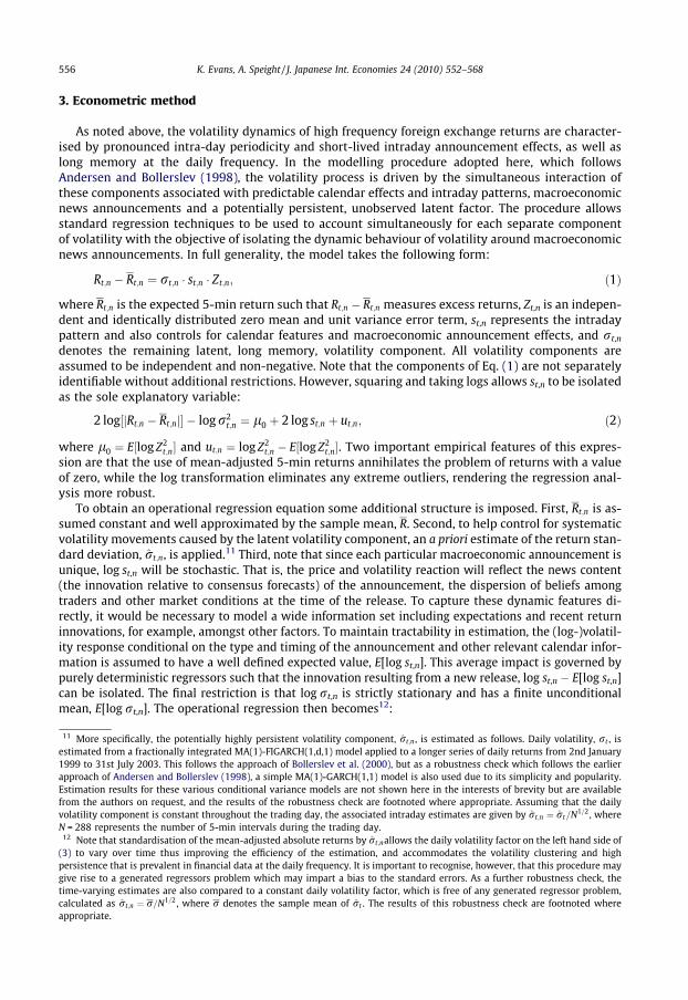
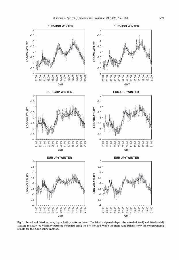
The relative empirical success of the intraday volatility models described in the preceding sectionin modelling the intra-day periodicity in exchange rate volatility may be readily judged by comparingthe fitted patterns to the corresponding sample average patterns.18 Fig. 1 therefore shows the fitted

16 Based on close inspection of the data and the underlying intraday patterns, the Tokyo opening effect is afforded a linearresponse (P = 1) beginning at 00:05 GMT and lasting until 00:30 GMT (X = 6) with the effect fading to zero at 00:35 GMT (p(X) = 0).Identical structure applies to the Hong Kong, Singapore and Malaysia opening effect but the effect begins an hour later at 01:05GMT. To account for a Monday morning slowdown, when traders in Sydney and Wellington are the only participants active in themarket, a second order polynomial (P = 2) is imposed from 21:05 GMT to 23:00 GMT (X = 23) with the restriction that p(X) = 0.Similarly, a Friday night slowdown, when US traders are the only active group, is also modelled by a second order polynomial.Based on the plots in Figure 1, this effect begins at 17:05 GMT in winter time and lasts until 21:00 GMT (X = 47) with the start ofthe effect shifted by 1 h to 16:05 GMT (X = 59) during DST. For this polynomial the restriction that p(0) = 0 ensures that there is nostep away from the intraday pattern at the impact of the event. The leftward shift of the intraday pattern by one hour during DSTgives rise to a hiatus between the close of trading in the US and the opening of trading in Wellington and this is accommodated forby a second order polynomial for each day during DST beginning at 19:05 GMT and lasting until 21:00 GMT (X = 23) with therestrictions p(X) = 0 and p(0) = 0 imposed. The final calendar effect is a winter slowdown which occurs for EUR–USD only, wherebyvolatility tends to be lower in the early part of the trading day and this effect is accounted for by a second order polynomialbeginning at 21:05 GMT on days during winter time lasting until 00:00 GMT (X = 35). The effect of the winter slowdownpolynomial is restricted to reach zero at 00:00 GMT (p(X) = 0).

17 More specifically, and following the findings of Andersen and Bollerslev (1998), Andersen et al. (2000) and Bollerslev et al.(2000), the average volatility dynamics in response to macroeconomic news announcements are approximated by a third-orderpolynomial restricted to equal zero at the end of the response horizon, as represented by P = 3 and X = 12. Each announcement hasa fixed response horizon of one hour (X = 12) except interest rate announcements from the FOMC and the Employment Report,which are afforded a 2 h horizon based on visual inspection of plots of their influence. To calculate this elongated 2 h responsewhilst retaining the benchmark pattern, the s variable is allowed to progress only by a (12/24) fraction of a unit per 5-min interval,rather than a full unit. This time deformation technique stretches the event time scale so that it conforms to the desired horizon.The response pattern is then fixed according to these estimates, leaving kk as the only free parameter to be estimated, whichmeasures the degree to which the event loads onto this pattern.

18 Coefficient estimates and their associated robust t statistics for Eq. (3) in conjunction with the FFF and cubic spline approaches tomodelling the intraday volatility pattern given by Eqs. (4) and (5), respectively, are suppressed here in the interests of brevity but areavailable from the authors on request. Since there is little economic interpretation to be gained from these parameter estimates, they arenot discussed further in the text, and we focus instead on the more easily interpreted plots of the actual and fitted log-volatility seriesand concentrate our discussion on the primary issue of interest, namely the volatility response to macroeconomic announcements.

EUR-USD WINTER

-4

-3.5

-3

-2.5

-2

-1.5

-1

-0.5

0

21:00

23:00

01:00

03:00

05:00

07:00

09:00

11:00

13:00

15:00

17:00

19:00

21:00

GMT

LOG

-VO

LATI

LITY

EUR-USD WINTER

-4

-3.5

-3

-2.5

-2

-1.5

-1

-0.5

0

21:00

23:00

01:00

03:00

05:00

07:00

09:00

11:00

13:00

15:00

17:00

19:00

21:00

GMT

LOG

-VO

LATI

LITY

EUR-GBP WINTER

-4

-3.5

-3

-2.5

-2

-1.5

-1

-0.5

0

21:00

23:00

01:00

03:00

05:00

07:00

09:00

11:00

13:00

15:00

17:00

19:00

21:00

GMT

LOG

-VO

LATI

LITY

EUR-GBP WINTER

-4

-3.5

-3

-2.5

-2

-1.5

-1

-0.5

0

21:00

23:00

01:00

03:00

05:00

07:00

09:00

11:00

13:00

15:00

17:00

19:00

21:00

GMT

LOG

-VO

LATI

LITY

EUR-JPY WINTER

-4

-3.5

-3

-2.5

-2

-1.5

-1

-0.5

0

21:00

23:00

01:00

03:00

05:00

07:00

09:00

11:00

13:00

15:00

17:00

19:00

21:00

GMT

LOG

-VO

LATI

LITY

EUR-JPY WINTER

-4

-3.5

-3

-2.5

-2

-1.5

-1

-0.5

0

21:00

23:00

01:00

03:00

05:00

07:00

09:00

11:00

13:00

15:00

17:00

19:00

21:00

GMT

LOG

-VO

LATI

LITY

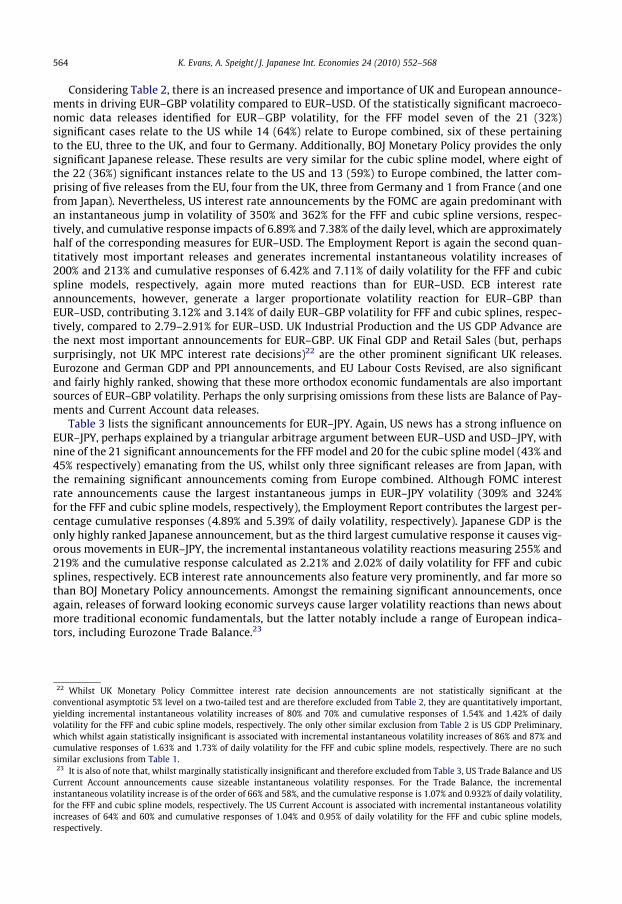
Fig. 1. Actual and fitted intraday log-volatility patterns. Notes: The left-hand panels depict the actual (dotted) and fitted (solid)average intraday log-volatility patterns modelled using the FFF method, while the right hand panels show the correspondingresults for the cubic spline method.



(solid line) and average actual (dotted line) intraday log-volatility pattern for each currency pairing, forthe FFF method in the left-hand panels and the alternative cubic spline method in the right hand pan-els.19 The smooth cyclical nature of the FFF pattern is clearly evident in the left-hand panel plots, andcaptures the rise in volatility when Sydney, Wellington and Tokyo traders are active, then a declinethrough the afternoon in Tokyo before rising again as European traders commence trading. The slow-down in volatility in the morning in the UK and Europe is also apparent, along with a subsequent in-crease to a peak when UK and US trading activity overlaps and then a steady decline through the USafternoon. The Tokyo market opening effect at 00:00 GMT and the effect of the opening of markets inHong Kong, Singapore and Malaysia 1 h later are also clearly shown, being particularly pronounced forEUR–JPY. Superimposing the sample average log-volatility pattern onto the fitted patterns in Fig. 1clearly reveals the relative success of the models in capturing the intraday volatility dynamics, andthe fit is good for all currency pairs.

The corresponding patterns for the cubic spline intraday models in the right hand panels are ingeneral very similar but, with the flexibility of the positioning of the knots, an advantage of the cubicsplines over FFF is that it does not necessarily impose a smooth pattern on intraday volatility but al-lows sharp peaks and troughs. A clear example is the peak during morning trading in Europe and theUK. Although the sharpness of this peak does not diverge greatly from the FFF pattern, this feature maybe of more critical importance at times when the position of the knot at this peak coincides with amacroeconomic news announcement. The fit is particularly good for EUR–USD and EUR–JPY, whilstthe EUR–GBP patterns show wider dispersion. Whilst both the FFF and cubic spline functions showaccurate fits, the cubic spline patterns appear to fit marginally better at the knot positions. The actuallog-volatility patterns in Fig. 1 also provide some initial evidence of the influence of scheduled mac-roeconomic news announcements on volatility. The first plot in the first column of Fig. 1, for example,shows clear spikes for EUR–USD volatility during intervals ending at 12:35, 13:35, 14:05 and 15:05GMT, times that correspond exactly with regularly scheduled announcements of US macroeconomicindicators at 8:30 and 10:00 Eastern Standard Time (EST).

In order to assess the relative importance of each individual macroeconomic announcement, and asdescribed in the previous section, the average effect of all US macroeconomic announcements are con-trolled for throughout while estimating the marginal impact of the release under investigation.20 Inthe case of assessing a US macroeconomic announcement, the release in question is removed from thecontrol group in the empirical estimation of the average effect of all US announcements. Tables 1–3 re-port the resulting coefficient estimates, robust t statistics, the percentage instantaneous jump in volatil-ity, and the cumulative effect on volatility over the response horizon as a percentage of the median dailycumulative absolute returns for all announcements showing a statistically significant positive estimatedloading coefficient,kk.21 These significant announcements are ordered in the tables by their contributionto daily returns variability.

19 The log-volatility patterns illustrated are for winter time GMT only in order to ease diagrammatic comparison, the plots forsummer time for EUR–USD and EUR–GBP being shifted rightwards by 1 h and exhibiting slightly elevated volatility, but areotherwise identical qualitatively.

20 Specifically, the third-order polynomial representation of the volatility pattern following a US macroeconomic announcementis determined by pðsÞ ¼ /0½1� ðs=12Þ3� þ /1s½1� ðs=12Þ2� þ /2s2½1� ðs=12Þ� for s ¼ 0;1;2; . . . ;12. This pattern is calibrated byfitting the three polynomial parameters for the 37 US announcements combined in Eqs. ((4); FFF) and ((5); CS) under therestriction k = 1, for each of the three bilateral exchange rates relative to the EUR. The resulting estimates for ð/0;/1;/2Þ are: USD–FFF (1.2206,�0.4166, 0.0555), USD–CS (1.2498, �0.4093, 0.0543); GBP–FFF (0.6387, �0.1043, 0.0048), GBP–CS (0.6625, �0.1100,0.0065); JPY–FFF (0.6994, �0.2199, 0.0304), JPY–CS (0.7224, �0.2258, 0.0319).

21 Significant announcements are selected as those reporting a loading parameter statistically greater than zero at the 5% levelunder the null hypothesis of a zero loading coefficient at asymptotic significance levels using t-statistics generated using robuststandard errors; see Tables 1–3. Whilst not presented here in full, the results of an alternative version of the model in whichabsolute mean-adjusted returns are standardised using the sample mean of rt;n , and which thus ignores any temporal variation inthis volatility factor, have also been considered. Whilst this version of the model does nothing to alleviate heteroscedasticity at thedaily frequency, it ensures that there is no practical generated regressors problem, which may exist when using rt;n . The parameterestimates are largely unchanged and the qualitative features of the inference unaffected, so the use of rt;n does not, therefore, seemto give rise to a generated regressors problem. As a further robustness check, estimation results for both these versions of themodel that uses rt;n as the daily volatility factor generated from an orthodox MA(1)-GARCH(1,1) model, rather than its fractionallyintegrated counterpart, have also been considered. Again, parameter estimates and inferences are similar to those reported in thetables, and confirm that the intraday features described in the text are not influenced by the choice of the daily volatility measure.

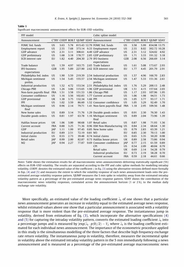
Table 1Significant macroeconomic announcement effects for EUR–USD volatility.

FFF model Cubic spline model

Announcement C’TRY COEFF ROB.T %JUMP %DAY Announcement C’TRY COEFF. ROB.T %JUMP %DAY

FOMC fed. funds US 3.63 5.78 815.43 12.79 FOMC fed. funds US 3.58 5.99 834.98 13.75Employment report US 2.55 7.68 373.14 9.33 Employment report US 2.55 8.02 392.72 10.28GDP advance US 2.31 3.11 308.61 4.49 GDP advance US 2.31 3.12 324.02 4.92GDP preliminary US 1.68 3.18 178.77 2.85 GDP preliminary US 1.71 3.33 191.32 3.18ECB interest rate EU 1.82 4.40 204.30 2.79 IFO business

expectationsGER 2.08 6.56 266.69 3.14

Trade balance US 1.59 4.97 163.75 2.65 Trade balance US 1.61 5.08 173.67 2.93IFO business

expectationsGER 1.95 5.89 227.90 2.62 ECB interest rate EU 1.77 4.45 201.79 2.91

Philadelphia fed. index US 1.90 5.59 219.39 2.54 Industrial production US 1.57 4.96 166.70 2.83Michigan sentiment

prelim.US 1.54 5.45 155.57 2.54 Michigan sentiment

prelim.US 1.47 5.33 151.36 2.61

Industrial production US 1.52 4.72 153.54 2.51 Philadelphia fed. index US 1.76 5.29 200.13 2.48Chicago PMI US 1.26 3.06 115.65 1.96 GDP provisional UK 1.51 4.15 157.64 2.03Non-farm payrolls final FRA 1.51 3.58 151.53 1.86 Chicago PMI US 1.17 2.93 107.96 1.95Consumer confidence US 1.16 3.56 102.83 1.77 Current account US 1.06 1.98 94.51 1.73GDP provisional UK 1.38 3.75 132.34 1.66 PPI US 1.05 3.77 93.17 1.71PPI US 1.02 3.59 86.60 1.52 Consumer confidence US 1.05 3.29 92.49 1.70Michigan sentiment

finalUS 0.96 2.14 79.71 1.41 Non-farm payrolls final FRA 1.18 2.95 109.56 1.48

New home sales US 0.89 3.14 71.76 1.29 Durable goods orders US 0.91 2.30 76.30 1.43Durable goods orders US 0.81 1.97 63.78 1.16 Michigan sentiment

finalUS 0.89 2.04 73.96 1.39

Halifax house prices UK 1.06 3.00 90.68 1.07 Retail sales US 0.87 1.98 71.93 1.36Current account FRA 0.88 3.25 71.36 0.96 ISM Non-Manufacturing US 0.84 2.34 68.64 1.30GDP JAP 1.11 1.99 97.45 0.85 New home sales US 0.79 2.83 63.39 1.21Industrial production EU 0.89 2.51 72.19 0.81 M3 EU 0.85 2.30 70.13 1.00Initial claims US 0.55 2.73 39.48 0.74 Initial claims US 0.65 3.35 50.20 0.98Retail sales JAP 0.99 2.00 82.87 0.73 Halifax house prices UK 0.89 2.58 73.86 0.94M2 JAP 0.94 2.27 77.87 0.69 Consumer confidence JAP 0.77 2.15 61.59 0.89

CPI US 0.54 2.09 40.04 0.79Retail sales UK 0.69 2.14 54.28 0.79Industrial production EU 0.73 2.19 58.28 0.70Current account FRA 0.59 2.18 44.61 0.66

Notes: Table shows the estimation results for all macroeconomic news announcements delivering statistically significant (5%)effects on EUR–USD volatility. The results are separated according to the FFF and cubic spline methods for modelling intradayvolatility. COEFF. denotes the estimated value of the coefficient k in Eq. (3) using the alternative versions defined more formallyin Eqs. (4) and (5) and measures the extent to which the volatility response of each news announcement loads onto the pre-estimated average volatility response pattern. %JUMP measures the 5 min spike in volatility away from the estimated intradayvolatility pattern as a percentage of the pre-estimated average news response pattern. %DAY shows the contribution of themacroeconomic news volatility responses, cumulated across the announcement horizon (1 or 2 h), to the median dailyexchange rate volatility.


More specifically, an estimated value of the loading coefficient kk of one shows that a particularnews announcement generates an increase in volatility equal to the estimated average news response,whilst estimated values above one show that a particular announcement is associated with a volatilityresponse that is more violent than the pre-estimated average response. The instantaneous jump involatility, derived from estimations of Eq. (3), which incorporate the alternative specifications (4)and (5) for capturing the intraday volatility pattern, converts the estimated loading coefficient kk intoa percentage jumps and is measured by ½expðkk � pð0Þ=2Þ � 1�, where kk is the loading coefficient esti-mated for each individual news announcement. The importance of the econometric procedure appliedin this study is the simultaneous modelling of the three factors that describe high frequency exchangerate return volatility. The instantaneous jump in volatility, therefore, measures the incremental spikein volatility above the estimated intraday volatility pattern in the 5 min immediately following a newsannouncement and is measured as a percentage of the pre-estimated average macroeconomic news


response. An estimated value of kk of 1, therefore, is synonymous with a spike in volatility awayfrom the estimated intraday volatility pattern equal to 100% of the pre-estimated average newsresponse.

The volatility response at the sth lag of the announcement window can be calculated as½expðkk � pðsÞ=2Þ � 1� such that the cumulative volatility response over the total announcement hori-zon (1 or 2 h) is given by

Ps¼0;X½expðkk � pðsÞ=2Þ � 1�, where p(s) is the predetermined volatility re-

sponse pattern. Tables 1–3 show the contribution of the cumulative volatility response over theannouncement horizon, for each news announcement, to daily exchange rate volatility. Dailyexchange rate volatility is measured for this purpose as the sum, over each day, of 5-min absolutereturns and so is similar to a measure of realised volatility. We take the median daily exchange ratevolatility over the days in the sample in an attempt to capture a representative day. The contributionof each news announcement to daily exchange rate volatility is then calculated as the ratio of thecumulative volatility response over the announcement horizon to the median daily exchange ratevolatility.

Table 1 shows clearly the dominance of US announcements in impacting EUR–USD volatility. Of thetotal 132 individual international macroeconomic announcements analyzed here, under the FFF model15 of the 25 significant announcements (or 60%) emanate from the US, while for the cubic spline mod-el 19 of the 29 significant announcements (or 66%) are from the US. Interest rate decisions announcedby the FOMC are by far the most important announcement, causing the largest instantaneous jump involatility measuring 815% and 835% for the FFF and cubic spline patterns, respectively, with the asso-ciated cumulative responses calculated as 12.79% and 13.75% of daily volatility. The sample includes aperiod when monetary policy authorities were lowering interest rates and when interest rateannouncements were surrounded by great uncertainty, making the timing of decisions to cut interestrates and the magnitude of the cuts very difficult to predict. In confirmation of the previous findings ofEderington and Lee (1993), Payne (1996), Andersen and Bollerslev (1998), Bollerslev et al. (2000),Andersen et al. (2003), the Employment Report is also an important indicator, causing immediatejumps in volatility of 373% and 393% for FFF and cubic spline versions, respectively, with the associ-ated cumulative volatility response measures of 9.33% and 10.28% of the median daily volatility,respectively. GDP figures are also crucial with the earlier Advance figures causing a more violent re-sponse than the Preliminary figures suggesting that traders learn from the Advance figures and areable to produce more accurate forecasts for the later Preliminary data. Among the remaining signifi-cant announcements, the US Trade Balance features very prominently, confirming the previous find-ings of Ederington and Lee (1993), Payne (1996), Andersen and Bollerslev (1998) and Andersen et al.(2003).

This list of the important macroeconomic news announcements, accompanied by many otherslisted in Table 1, is entirely as we would expect from conventional exchange rate determination the-ories. For example, the monetary model suggests that exchange rates are determined by relativemoney supplies, real incomes and nominal interest rates, whilst the sticky price monetary model al-lows short term overshooting of the exchange rate in compensation of stickiness in prices and output.Furthermore, the portfolio balance model suggests imperfect substitutability between domestic andforeign assets such that in response to differences in interest rates or expected rates of return, inves-tors shift their funds between foreign and domestic investments, thus influencing exchange rates.Also, the Mundell–Fleming large open economy macroeconomic model suggests a crucial role forthe trade balance in determining the exchange rate. Each of these approaches suggests current andanticipated values of fundamentals such as the money supply, output, interest rates and the trade bal-ance determine exchange rates. Assuming that information is fully incorporated into existing currencyvalues, exchange rate changes will be associated with announcements of information related to thesefundamentals.

However, consistent with the findings of Andersen et al. (2003), there remain a number of otherimportant US announcements that are not considered in the traditional exchange rate determinationtheories. Specifically, these are forward looking indices such as the Philadelphia Federal Reserve Index,the University of Michigan Sentiment Index (Preliminary and Final) and Chicago PMI. Aside from theireconomic content and forward looking nature, it is the timing of their release that causes substantialexchange rate volatility. These indices are released very early in each month and are typically the first

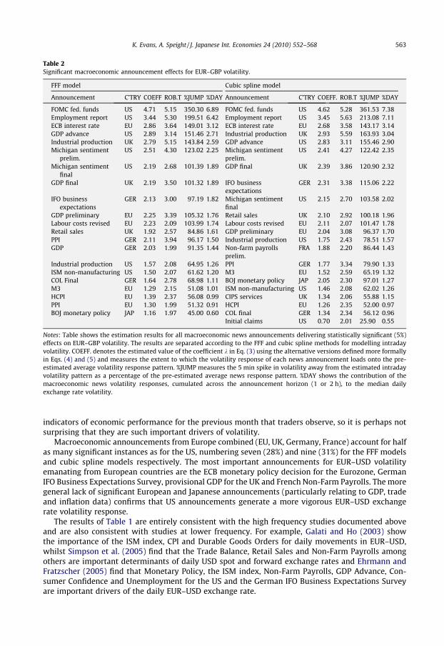
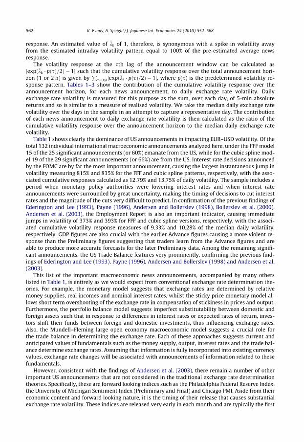
Table 2Significant macroeconomic announcement effects for EUR–GBP volatility.



FOMC fed. funds US 4.71 5.15 350.30 6.89 FOMC fed. funds US 4.62 5.28 361.53 7.38Employment report US 3.44 5.30 199.51 6.42 Employment report US 3.45 5.63 213.08 7.11ECB interest rate EU 2.86 3.64 149.01 3.12 ECB interest rate EU 2.68 3.58 143.17 3.14GDP advance US 2.89 3.14 151.46 2.71 Industrial production UK 2.93 5.59 163.93 3.04Industrial production UK 2.79 5.15 143.84 2.59 GDP advance US 2.83 3.11 155.46 2.90Michigan sentiment

prelim.US 2.51 4.30 123.02 2.25 Michigan sentiment

prelim.US 2.41 4.27 122.42 2.35

Michigan sentimentfinal

US 2.19 2.68 101.39 1.89 GDP final UK 2.39 3.86 120.90 2.32

GDP final UK 2.19 3.50 101.32 1.89 IFO businessexpectations

GER 2.31 3.38 115.06 2.22

IFO businessexpectations

GER 2.13 3.00 97.19 1.82 Michigan sentimentfinal

US 2.15 2.70 103.58 2.02

GDP preliminary EU 2.25 3.39 105.32 1.76 Retail sales UK 2.10 2.92 100.18 1.96Labour costs revised EU 2.23 2.09 103.99 1.74 Labour costs revised EU 2.11 2.07 101.47 1.78Retail sales UK 1.92 2.57 84.86 1.61 GDP preliminary EU 2.04 3.08 96.37 1.70PPI GER 2.11 3.94 96.17 1.50 Industrial production US 1.75 2.43 78.51 1.57GDP GER 2.03 1.99 91.35 1.44 Non-farm payrolls

prelim.FRA 1.88 2.20 86.44 1.43

Industrial production US 1.57 2.08 64.95 1.26 PPI GER 1.77 3.34 79.90 1.33ISM non-manufacturing US 1.50 2.07 61.62 1.20 M3 EU 1.52 2.59 65.19 1.32COL Final GER 1.64 2.78 68.98 1.11 BOJ monetary policy JAP 2.05 2.30 97.01 1.27M3 EU 1.29 2.15 51.08 1.01 ISM non-manufacturing US 1.46 2.08 62.02 1.26HCPI EU 1.39 2.37 56.08 0.99 CIPS services UK 1.34 2.06 55.88 1.15PPI EU 1.30 1.99 51.32 0.91 HCPI EU 1.26 2.35 52.00 0.97BOJ monetary policy JAP 1.16 1.97 45.00 0.60 COL final GER 1.34 2.34 56.12 0.96

Initial claims US 0.70 2.01 25.90 0.55

Notes: Table shows the estimation results for all macroeconomic news announcements delivering statistically significant (5%)effects on EUR–GBP volatility. The results are separated according to the FFF and cubic spline methods for modelling intradayvolatility. COEFF. denotes the estimated value of the coefficient k in Eq. (3) using the alternative versions defined more formallyin Eqs. (4) and (5) and measures the extent to which the volatility response of each news announcement loads onto the pre-estimated average volatility response pattern. %JUMP measures the 5 min spike in volatility away from the estimated intradayvolatility pattern as a percentage of the pre-estimated average news response pattern. %DAY shows the contribution of themacroeconomic news volatility responses, cumulated across the announcement horizon (1 or 2 h), to the median dailyexchange rate volatility.


indicators of economic performance for the previous month that traders observe, so it is perhaps notsurprising that they are such important drivers of volatility.

Macroeconomic announcements from Europe combined (EU, UK, Germany, France) account for halfas many significant instances as for the US, numbering seven (28%) and nine (31%) for the FFF modelsand cubic spline models respectively. The most important announcements for EUR–USD volatilityemanating from European countries are the ECB monetary policy decision for the Eurozone, GermanIFO Business Expectations Survey, provisional GDP for the UK and French Non-Farm Payrolls. The moregeneral lack of significant European and Japanese announcements (particularly relating to GDP, tradeand inflation data) confirms that US announcements generate a more vigorous EUR–USD exchangerate volatility response.

The results of Table 1 are entirely consistent with the high frequency studies documented aboveand are also consistent with studies at lower frequency. For example, Galati and Ho (2003) showthe importance of the ISM index, CPI and Durable Goods Orders for daily movements in EUR–USD,whilst Simpson et al. (2005) find that the Trade Balance, Retail Sales and Non-Farm Payrolls amongothers are important determinants of daily USD spot and forward exchange rates and Ehrmann andFratzscher (2005) find that Monetary Policy, the ISM index, Non-Farm Payrolls, GDP Advance, Con-sumer Confidence and Unemployment for the US and the German IFO Business Expectations Surveyare important drivers of the daily EUR–USD exchange rate.


Considering Table 2, there is an increased presence and importance of UK and European announce-ments in driving EUR–GBP volatility compared to EUR–USD. Of the statistically significant macroeco-nomic data releases identified for EUR�GBP volatility, for the FFF model seven of the 21 (32%)significant cases relate to the US while 14 (64%) relate to Europe combined, six of these pertainingto the EU, three to the UK, and four to Germany. Additionally, BOJ Monetary Policy provides the onlysignificant Japanese release. These results are very similar for the cubic spline model, where eight ofthe 22 (36%) significant instances relate to the US and 13 (59%) to Europe combined, the latter com-prising of five releases from the EU, four from the UK, three from Germany and 1 from France (and onefrom Japan). Nevertheless, US interest rate announcements by the FOMC are again predominant withan instantaneous jump in volatility of 350% and 362% for the FFF and cubic spline versions, respec-tively, and cumulative response impacts of 6.89% and 7.38% of the daily level, which are approximatelyhalf of the corresponding measures for EUR–USD. The Employment Report is again the second quan-titatively most important releases and generates incremental instantaneous volatility increases of200% and 213% and cumulative responses of 6.42% and 7.11% of daily volatility for the FFF and cubicspline models, respectively, again more muted reactions than for EUR–USD. ECB interest rateannouncements, however, generate a larger proportionate volatility reaction for EUR–GBP thanEUR–USD, contributing 3.12% and 3.14% of daily EUR–GBP volatility for FFF and cubic splines, respec-tively, compared to 2.79–2.91% for EUR–USD. UK Industrial Production and the US GDP Advance arethe next most important announcements for EUR–GBP. UK Final GDP and Retail Sales (but, perhapssurprisingly, not UK MPC interest rate decisions)22 are the other prominent significant UK releases.Eurozone and German GDP and PPI announcements, and EU Labour Costs Revised, are also significantand fairly highly ranked, showing that these more orthodox economic fundamentals are also importantsources of EUR–GBP volatility. Perhaps the only surprising omissions from these lists are Balance of Pay-ments and Current Account data releases.

Table 3 lists the significant announcements for EUR–JPY. Again, US news has a strong influence onEUR–JPY, perhaps explained by a triangular arbitrage argument between EUR–USD and USD–JPY, withnine of the 21 significant announcements for the FFF model and 20 for the cubic spline model (43% and45% respectively) emanating from the US, whilst only three significant releases are from Japan, withthe remaining significant announcements coming from Europe combined. Although FOMC interestrate announcements cause the largest instantaneous jumps in EUR–JPY volatility (309% and 324%for the FFF and cubic spline models, respectively), the Employment Report contributes the largest per-centage cumulative responses (4.89% and 5.39% of daily volatility, respectively). Japanese GDP is theonly highly ranked Japanese announcement, but as the third largest cumulative response it causes vig-orous movements in EUR–JPY, the incremental instantaneous volatility reactions measuring 255% and219% and the cumulative response calculated as 2.21% and 2.02% of daily volatility for FFF and cubicsplines, respectively. ECB interest rate announcements also feature very prominently, and far more sothan BOJ Monetary Policy announcements. Amongst the remaining significant announcements, onceagain, releases of forward looking economic surveys cause larger volatility reactions than news aboutmore traditional economic fundamentals, but the latter notably include a range of European indica-tors, including Eurozone Trade Balance.23

22 Whilst UK Monetary Policy Committee interest rate decision announcements are not statistically significant at theconventional asymptotic 5% level on a two-tailed test and are therefore excluded from Table 2, they are quantitatively important,yielding incremental instantaneous volatility increases of 80% and 70% and cumulative responses of 1.54% and 1.42% of dailyvolatility for the FFF and cubic spline models, respectively. The only other similar exclusion from Table 2 is US GDP Preliminary,which whilst again statistically insignificant is associated with incremental instantaneous volatility increases of 86% and 87% andcumulative responses of 1.63% and 1.73% of daily volatility for the FFF and cubic spline models, respectively. There are no suchsimilar exclusions from Table 1.

23 It is also of note that, whilst marginally statistically insignificant and therefore excluded from Table 3, US Trade Balance and USCurrent Account announcements cause sizeable instantaneous volatility responses. For the Trade Balance, the incrementalinstantaneous volatility increase is of the order of 66% and 58%, and the cumulative response is 1.07% and 0.932% of daily volatility,for the FFF and cubic spline models, respectively. The US Current Account is associated with incremental instantaneous volatilityincreases of 64% and 60% and cumulative responses of 1.04% and 0.95% of daily volatility for the FFF and cubic spline models,respectively.

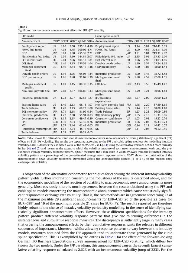
Table 3Significant macroeconomic announcement effects for EUR–JPY volatility.



Employment report US 3.10 5.50 195.19 4.89 Employment report US 3.14 5.84 210.41 5.39FOMC fed. funds US 4.03 4.45 309.02 4.71 FOMC fed. funds US 4.00 4.65 324.11 5.06GDP JAP 3.63 5.30 255.38 2.21 GDP JAP 3.21 5.04 219.31 2.02Philadelphia fed. index US 2.56 5.30 144.84 2.07 Philadelphia fed. index US 2.35 5.04 133.83 2.00ECB interest rate EU 2.04 2.96 104.13 1.81 ECB interest rate EU 1.96 2.98 103.03 1.86COL final GER 2.46 3.95 136.52 1.64 Durable goods orders US 1.99 3.54 105.24 1.62Michigan sentiment

finalUS 1.96 2.54 98.12 1.48 GDP preliminary US 1.90 3.05 98.90 1.54

Durable goods orders US 1.91 3.25 95.05 1.44 Industrial production UK 1.90 3.44 98.72 1.53GDP preliminary US 1.86 2.90 91.67 1.39 Michigan sentiment

finalUS 1.88 2.52 97.08 1.51

Michigan sentimentprelim.

US 1.81 3.15 88.39 1.35 COL final GER 2.13 3.50 115.49 1.47

Non-farm payrolls final FRA 2.08 2.67 106.86 1.33 Michigan sentimentprelim.

US 1.79 3.21 90.96 1.43

Industrial production UK 1.72 2.97 82.58 1.27 IFO businessexpectations

GER 1.57 2.00 76.00 1.22

Existing home sales US 1.49 2.13 68.18 1.07 Non-farm payrolls final FRA 1.75 2.29 87.89 1.15Trade balance EU 1.49 3.73 68.23 1.00 Existing home sales US 1.44 2.15 68.08 1.10BOJ monetary policy JAP 1.71 2.18 81.99 0.84 Trade balance EU 1.23 3.23 56.09 0.86Industrial production EU 1.27 2.38 55.94 0.83 BOJ monetary policy JAP 1.65 2.18 81.31 0.86Consumer confidence US 1.15 2.18 49.47 0.80 Consumer confidence US 1.03 2.03 45.22 0.76PPI GER 1.30 2.93 57.45 0.76 Industrial production EU 1.06 2.07 46.43 0.73M2 JAP 1.37 2.44 61.42 0.65 PPI GER 0.94 2.11 40.42 0.57Household consumption FRA 1.12 2.24 48.12 0.65 M2 JAP 1.11 2.02 49.12 0.55Trade balance JAP 1.33 2.12 59.29 0.63

Notes: Table shows the estimation results for all macroeconomic news announcements delivering statistically significant (5%)effects on EUR–JPY volatility. The results are separated according to the FFF and cubic spline methods for modelling intradayvolatility. COEFF. denotes the estimated value of the coefficient k in Eq. (3) using the alternative versions defined more formallyin Eqs. (4) and (5) and measures the extent to which the volatility response of each news announcement loads onto the pre-estimated average volatility response pattern. %JUMP measures the 5 min spike in volatility away from the estimated intradayvolatility pattern as a percentage of the pre-estimated average news response pattern. %DAY shows the contribution of themacroeconomic news volatility responses, cumulated across the announcement horizon (1 or 2 h), to the median dailyexchange rate volatility.


Comparison of the alternative econometric techniques for capturing the inherent intraday volatilitypattern yields further information concerning the robustness of the results described above, and forthe econometric modelling of the reaction of volatility to macroeconomic news announcements moregenerally. Most obviously, there is much agreement between the results obtained using the FFF andcubic spline models concerning the macroeconomic announcements which cause statistically signifi-cant responses in exchange rate volatility. That is, the two methods are in agreement concerning 22 ofthe maximum possible 29 significant announcements for EUR–USD, 20 of the possible 22 cases forEUR–GBP, and 19 of the maximum possible 21 cases for EUR–JPY. The results reported are thereforehighly robust to the choice of intraday volatility periodicity modelling, in the sense of identifying sta-tistically significant announcement effects. However, these different specifications for the intradaypattern produce different volatility response patterns that give rise to striking differences in theinstantaneous and cumulative response measures. The discrepancy is sufficiently large in many casesthat ordering the announcement effects by their cumulative responses ranks the releases in differentsequences of importance. Moreover, whilst allowing response patterns to vary between the intradaymodels, measures obtained form the FFF approach tend to understate those generated by the cubicspline specification. This is exemplified by the entries in Table 1 for the effect of the forward-lookingGerman IFO Business Expectations survey announcement for EUR–USD volatility, which differs be-tween the two models. Under the FFF paradigm, this announcement causes the seventh largest cumu-lative volatility response calculated as 2.62% with an instantaneous volatility jump of 223%. For the


cubic spline approach, however, this same announcement generates the fifth largest cumulative vol-atility response measuring 3.14% at the daily level and corresponding to an incremental instantaneousvolatility response of 267%. This discrepancy between the volatility response measures also holdsmore generally, with the FFF model results understating the percentage cumulative volatility responsecompared to the cubic spline model in almost all cases in Tables 1–3. Thus, whilst the identification ofsignificant macroeconomic announcements for exchange rate volatility is not sensitive to the choice ofintraday volatility specification, the quantification of that volatility response is sensitive to that choice.

Finally, further evidence to support the use of the cubic spline approach is presented by theR-squared measures of the regressions. Although there is an individual regression for each newsannouncement, the associated R-squared measures fluctuate very little. For the FFF method, adjustedR-squared measures are 0.0378, 0.0201 and 0.0200 for EUR–USD, EUR–GBP and EUR–JPY, respectively.The corresponding figures for the cubic spline method are slightly higher at 0.0382, 0.0206 and 0.0203showing some evidence that the cubic spline method provides a superior fit to the data. In general, theadjusted R-squared measures are quite small, illustrating the difficulty in accurately modelling thedynamics of high frequency exchange rate returns over a 19-month sample. Despite the low R-squaredvalues, the econometric techniques applied in this study show strong evidence that high frequencyexchange rate volatility follows a clear intraday pattern and explains the importance of macroeco-nomic announcements for intraday volatility in two ways. First, there is a substantial, immediate‘jump’ away from the intraday volatility pattern (instantaneous jump) following some important re-leases. Second, this increased volatility persists over a 1 or 2 h announcement horizon to contributesubstantially to daily volatility (contribution of cumulative volatility response to daily volatility).

5. Conclusions

This paper has sought to provide a comprehensive characterisation of Euro exchange rate volatility,focusing on the volatility response to a range of international macroeconomic announcements. Thepaper contributes to the literature in several ways. First, it uses 5-min bid-ask quotes of the Euroagainst the US Dollar, UK Pound sterling and Japanese Yen, which constitutes a new market thathas yet to be investigated. Second, it considers a far wider range of announcements across countriesand economic conditions than has been considered hitherto in the literature, and against a turbulenteconomic and geopolitical background. Third, the complexity of the volatility response to individualmacroeconomic announcements is assessed through volatility response functions rather than the sig-nificance of simple dummy variables for categories of announcement type as typically applied in theprevious literature. Fourth, the empirical methodology which permits simultaneous modelling ofthese announcement effects together with long-memory features and intra-day periodicity utilisestwo approaches to the modelling of the latter, namely the conventional FFF approach and an alterna-tive method using cubic splines.

The largest reactions of volatility across the three exchange rates are found to occur in response toUS announcements. In a sample period of poor global economic performance, the decisions of theFOMC regarding US interest rates generate the largest instantaneous jumps in volatility and oftenthe largest cumulative response over the period immediately following the announcement. Interestrate decisions by the ECB also feature prominently showing that monetary policy decisions are animportant source of exchange rate volatility over the sample, which may have been confounded dur-ing the sample period by the ECB’s monetary policy reactions being difficult to predict accurately. Inconfirmation of previous studies, indicators of real activity such as the US Employment Report andGDP also cause dramatic price reactions, whilst similar measures for the UK (including UK IndustrialProduction), Eurozone, Germany and Japan are among the highest ranking non-US announcements.The US Trade Balance is also found to be important, causing a larger EUR–USD reaction than US infla-tion data. Aside from such traditional macroeconomic information, forward looking indicators and re-gional economic surveys are found to play a crucial and interesting role. These releases include thePhiladelphia Federal Reserve Index, University of Michigan Consumer Sentiment Index, ChicagoPurchasing Managers Index, Consumer Confidence Index and Institute of Supply Management Indexfor the US, and the IFO Business Expectations Index for Germany. The timing of these announcements


is such that they are the first indicators of macroeconomic performance for a particular month thattraders observe, and such releases are therefore likely to generate larger price reactions. By learningfrom this early information, subsequent announcements pertaining to the same month can be forecastwith greater accuracy, such that subsequent announcements cause smaller deviations from expecta-tions and hence do not cause such dramatic volatility movements.

There are several possible avenues for further research. The data sample used in this study is par-ticularly interesting as it covers a period of economic turbulence, geopolitical tension and episodes ofmonetary policy easing. However, it would be appealing to extend the sample to cover differentphases of the business cycle in order to analyse whether markets react symmetrically to good andbad news and whether this reaction is symmetric during economic expansions and contractions. Gi-ven the importance of monetary policy reactions identified, it would also be interesting to relate anysuch asymmetric news effects to the reaction functions of monetary policy authorities. Finally, in thecontext of realised volatility models, the econometrics of quantifying and explaining volatility ‘jumps’is an innovative area of empirical finance research and such ‘jump’ contributions to total volatility maybe linked to macroeconomic announcements and news given the findings reported here.

References

Almeida, A., Goodhart, C., Payne, R., 1998. The effects of macroeconomic news on high frequency exchange rate behaviour.Journal of Financial and Quantitative Analysis 33, 383–408.

Andersen, T.G., Bollerslev, T., 1997a. Intraday periodicity and volatility persistence in financial markets. Journal of EmpiricalFinance 4, 115–158.

Andersen, T.G., Bollerslev, T., 1997b. Heterogeneous information arrivals and return volatility dynamics: uncovering the long-run in high frequency returns. Journal of Finance 52, 975–1005.

Andersen, T.G., Bollerslev, T., 1998. Deutsche mark-dollar volatility: intraday activity patterns, macroeconomic announcements,and longer run dependencies. Journal of Finance 53, 219–265.

Andersen, T.G., Bollerslev, T., Cai, J., 2000. Intraday and interday volatility in the Japanese stock market. Journal of InternationalFinancial Markets, Institutions and Money 10, 107–130.

Andersen, T.G., Bollerslev, T., Diebold, F.X., Vega, C., 2003. Micro effects of macro announcements: real-time price discovery inforeign exchange. American Economic Review 93, 38–62.

Bauwens, L., Omrane, W.B., Giot, P., 2005. News announcements, market activity and volatility in the euro/dollar foreignexchange market. Journal of International Money and Finance 24, 1108–1125.

Bollerslev, T., Domowitz, I., 1993. Trading patterns and prices in the interbank foreign exchange market. Journal of Finance 48,1421–1443.

Bollerslev, T., Cai, J., Song, F.M., 2000. Intraday periodicity, long memory volatility, and macroeconomic announcement effects inthe US treasury bond market. Journal of Empirical Finance 7, 37–55.

Chang, Y., Taylor, S.J., 2003. Information arrivals and intraday exchange rate volatility. Journal of International FinancialMarkets, Institutions and Money 13, 85–112.

DeGennaro, R.P., Shrieves, R.E., 1997. Public information releases, private information arrival and volatility in the foreignexchange market. Journal of Empirical Finance 4, 295–315.

Ederington, L.H., Lee, J.H., 1993. How markets process information: news releases and volatility. Journal of Finance 48, 1161–1191.

Ehrmann, M., Fratzscher, M., 2005. Exchange rates and fundamentals: new evidence from real-time data. Journal ofInternational Money and Finance 24, 317–341.

Engle, R., Russell, J., 1998. Autoregressive conditional duration: a new model for irregularly spaced transaction data.Econometrica 66, 1127–1162.

Galati, G., Ho, C., 2003. Macroeconomic news and the euro/dollar exchange rate. Economic Notes by Banca Monte dei Paschi diSiena SpA 32, 371–398.

Gençay, R., Selçuk, F., Whitcher, B., 2001. Differentiating intraday seasonalities through wavelet multi-scaling. Physica A 289,543–556.

Giot, P., 2005. Market risk models for intraday data. European Journal of Finance 11, 309–324.Hashimoto, Y., Ito, T., 2010. Effects of Japanese macroeconomic statistic announcements on the dollar/yen exchange rate: high

resolution picture. Journal of the Japanese and International Economies 24, 334–354.Hashimoto, Y., Ito, T., Ohnishi, T., Takayasu, M., Takayasu, H. and Watanabe, T., 2008. Random Walk or a Run: Market

Microstructure Analysis of the Foreign Exchange Rate Movements Based on Conditional Probability. NBER Working Paper14160.

Ito, T., Hashimoto, Y., 2006a. Intraday seasonality in activities of the foreign exchange markets: evidence from the electronicbroking system. Journal of the Japanese and International Economies 20, 637–664.

Ito, T., Hashimoto, Y., 2006b. Price impacts of Deals and Predictability of the Exchange Rate Movements. NBER Working Paper12682.

Jansen, D.-J., De Haan, J., 2005. Talking heads: the effects of ECB statements on the euro-dollar exchange rate. Journal ofInternational Money and Finance 24, 343–361.

Payne, R., 1996. Announcement Effects and Seasonality in the Intraday Foreign Exchange Market. Discussion Paper 238,Financial Markets Group, London School of Economics.


Sager, M.J., Taylor, M.P., 2004. The impact of European Central Bank Governing Council announcements on the foreign exchangemarket: a microstructural analysis. Journal of International Money and Finance 23, 1043–1051.

Simpson, M.W., Ramchander, S., Chaudhry, M., 2005. The impact of macroeconomic surprises on spot and forward foreignexchange markets. Journal of International Money and Finance 24, 693–718.

Taylor, N., 2004a. Trading intensity, volatility, and arbitrage activity. Journal of Banking and Finance 28, 1137–1162.Taylor, N., 2004b. Modeling discontinuous periodic conditional volatility: evidence from the commodity futures market. Journal

of Futures Markets 24, 805–834.Zhang, M., Russell, J., Tsay, R., 2001. A nonlinear autoregressive conditional duration model with applications to financial

transaction data. Journal of Econometrics 61, 179–207.

international macroeconomic announcements and intraday euro exchange rate volatility

Documents