interaction of atmospheric chemistry and climate and its impact on stratospheric ozone

C. Schnadt Æ M. Dameris Æ M.Ponater

R. Hein Æ V. Grewe Æ B. Steil

Interaction of atmospheric chemistry andclimate and its impact on stratospheric ozone

Received: 8 March 2001 /Accepted: 21 June 2001 / Published online: 7 December 2001� Springer-Verlag 2001

Abstract The interactively coupled chemistry-climatemodel ECHAM4.L39(DLR)/CHEM is employed insensitivity calculations to investigate feedback mecha-nisms of dynamic, chemical, and radiative processes.Two multi-year model simulations are carried out,which represent recent atmospheric conditions. It isshown that the model is able to reproduce observedfeatures and trends with respect to dynamics andchemistry of the troposphere and lower stratosphere. Inpolar regions it is demonstrated that an increased per-sistence of the winter vortices is mainly due to enhancedgreenhouse gas mixing ratios and to reduced ozoneconcentration in the lower stratosphere. An additionalsensitivity simulation is investigated, concerning a pos-sible future development of the chemical composition ofthe atmosphere and climate. The model results in theSouthern Hemisphere indicate that the adopted furtherincrease of greenhouse gas mixing ratios leads to anintensified radiative cooling in the lower stratosphere.Therefore, Antarctic ozone depletion slightly increasesdue to a larger PSC activity, although stratosphericchlorine is reduced. Interestingly, the behavior in theNorthern Hemisphere is different. During winter, anenhanced activity of planetary waves yields a more dis-turbed stratospheric vortex. This ‘‘dynamical heating’’compensates the additional radiative cooling due toenhanced greenhouse gas concentrations in the polarregion. In connection with reduced stratospheric chlo-rine loading, the ozone layer clearly recovers.

1 Introduction

Extensive investigations have been made of how changesof the concentrations of radiatively and chemically ac-tive gases affect the radiative, chemical, and dynamicbehavior of the stratosphere and their feedback on cli-mate (e.g. Ramanathan et al. 1976; Groves et al. 1978;Boughner 1978; Fels et al. 1980; Shine 1986, 1989). Ofparticular interest has been the mutual effect of ozoneand climate change (e.g. Cariolle et al. 1990; Dameriset al. 1991; Pitari et al. 1992; Graf et al. 1998). Increasedattention has been focused recently on the substantialreduction of the ozone layer during the past two decadesand its relevance for climate change (e.g. Bengtsson et al.1999; Forster 1999; Randel and Wu 1999; Langematz2000). Currently, the timing and the completeness ofozone recovery over the coming years and decades isvery uncertain. On one hand, the recovery of the ozonelayer will depend on the chlorine loading of the strato-sphere, which is expected to decrease during the nextdecades (WMO 1999). On the other hand, climatechange, which is expected as a consequence of the an-ticipated further increase of greenhouse gas concentra-tions, may become relevant for atmospheric ozonechemistry in the future (e.g. Shindell et al. 1998; Danilinet al. 1998; Dameris et al. 1998; Austin et al. 2000).Austin et al. (1992) were the first to discuss the possi-bility of an Arctic ozone hole in a doubled CO2 atmo-sphere as a consequence of a reduced lower stratospherictemperature. Their model study clearly indicated that astrong radiative perturbation in the stratosphere has adistinct effect on ozone destruction. Therefore, investi-gating the interaction of climate change and of ozonerecovery is one of the major scientific challenges ofpresent day climate research.

In fact, long-term temperature measurements show astatistically significant warming of lower troposphericlayers and a pronounced cooling of the stratosphere.Both trends can be partly explained by the observed

Climate Dynamics (2002) 18: 501–517DOI 10.1007/s00382-001-0190-z

C. Schnadt Æ M. Dameris (&) Æ M. PonaterR. Hein Æ V. GreweDLR Institut fur Physik der Atmosphare,Oberpfaffenhofen,82230 Weßling, GermanyE-mail: [email protected]

B. SteilMax-Planck-Institut fur Chemie,Abteilung Luftchemie,55020 Mainz, Germany

increase of greenhouse gas concentrations during thelast century (e.g. Steinbrecht et al. 1998; Pawson et al.1998; Kivi et al. 1999; Santer et al. 1999). The coolingof the Arctic and Antarctic stratosphere is clearly en-hanced due to ozone depletion itself, particularly in latewinter and spring, which is obvious from multi-yeardata records (e.g. Randel and Wu 1999; WMO 1999).These temperature changes are associated with an in-creased stability of the wintertime stratospheric polarvortices and a poleward shift of the westerly wind beltsnear the surface (Hartmann et al. 2000). As other recentfindings point out, the modelling of the atmosphericsystem must not only consider the feedback mecha-nisms of dynamic, chemical, and radiation processes inthe stratosphere as a secluded system, but it must alsotake into account the dynamic coupling between thetroposphere and the stratosphere. This dynamic linkand its importance for the genesis of natural and an-thropogenic climate variations have been intensivelyanalyzed in a series of investigations (e.g. Perlwitz andGraf 1995; Perlwitz et al. 2000). For example, it wasshown that winter seasons characterized by either astrong or a weak stratospheric vortex are associatedwith different tropospheric circulation regimes. On theother hand, upward propagating planetary wavesoriginating in the troposphere have a dominant influ-ence on the dynamic behavior of the stratosphere dueto wave breaking and momentum deposition (e.g. An-drews et al. 1987).

In this study the interactively coupled chemistry-cli-mate model ECHAM4.L39(DLR)/CHEM (hereafterreferred to as E39/C) is used to obtain further knowl-edge about dynamic and chemical key processes in-volved in the recent changes of tropospheric and lowerstratospheric temperature and chemical composition,and to provide indications for the possible developmentof climate and its impact on the ozone layer in the nearfuture. Considering the feedback between dynamic,chemical, and radiative processes establishes a clearconceptional progress for climate change studies com-pared with conventional general circulation models(GCMs), which use fixed climatological mean fields ofshort-lived radiatively active chemical species like ozone(e.g. Bengtsson et al. 1999) in the model’s radiativetransfer scheme. Furthermore, the application of achemistry model that considers relevant chemical speciesand reactions to describe upper troposphere and lowerstratosphere ozone chemistry (instead of much simplerapproaches with parameterized chemistry, e.g. Cariolleet al. 1990; Shindell et al. 1998) in multi-year simula-tions is another step forward to obtain a better under-standing of the reasons for observed changes of climateparameters and the chemical composition of the atmo-sphere.

Our aim is to identify and to investigate importantinteraction mechanisms between dynamic, chemical, andradiative processes in the lower stratosphere. Due totheir importance for polar stratospheric ozone, feedbackmechanisms in the polar stratosphere during winter and

spring are of particular interest. Thus their investigationconstitutes the essential part of this paper. The analysisis based on scenario calculations, which include thechanges of atmospheric composition during recentyears, mainly resulting from greenhouse gas concentra-tion increases and changes of stratospheric chlorineloading. By comparing these numerical experiments,changes of dominant interaction mechanisms and theirimpact on stratospheric ozone can be identified. At first,an adequate comparison between model results of multi-year integrations and respective long-term observationsforms the basis for the analysis of dynamic-chemicalinteraction mechanisms.This indicates the comprehen-siveness of our understanding of the atmospheric sys-tem, and it also shows the abilities and deficiencies of themodel system employed.

Such a comparison of model results to related ob-servations has shown that the model is able to describeimportant dynamic and chemical processes and to re-produce the seasonal and spatial distribution of relevantchemical species (Sect. 3.1) for recent atmospheric con-ditions (Hein et al. 2001, hereafter referred to as H2001).This scenario run will be designated ‘reference simula-tion’. Here, E39/C is used to investigate changes of dy-namics and chemistry in the past and future comparedwith this reference simulation. The work is subdividedinto two parts: first, an extended model valuation ispresented, which shows the model’s performance in re-producing observed stratospheric temperature, ozone,and water vapor trends of the 1980s. The second partdeals with dynamic and chemical changes that arise as aconsequence of enhanced greenhouse gas concentrationsand a slightly reduced stratospheric chlorine abundance(with respect to the reference simulation) in a near futurescenario.

In the following section a brief summary of the modeland the design of the experiments will be presented.Model results will be discussed and compared with ob-servations in Sect. 3. The radiative and dynamic pro-cesses, which are responsible for the behavior of themodel will be investigated in the subsequent section.Conclusions will be given in the last section.

2 Brief model description and design of experiments

2.1 The model

A detailed description of the chemistry-climate model E39/C, theused parameterisations, boundary conditions, as well as naturaland anthropogenic emissions was given in H2001. They also dis-cussed the main features of the model climatology. In this sectionthe model characteristics are briefly summarized.

The atmosphere GCM ECHAM4.L39(DLR) (E39) is appliedwith a horizontal resolution of T30, i.e. dynamic processes havean isotropic resolution of about 670 km. The correspondingGaussian transform latitude-longitude grid, on which the modelphysics, chemistry, and tracer transport are calculated, has a meshsize of 3.75�·3.75�. In the vertical, the model uses 39 layers (L39)from the surface up to the top layer centred at 10 hPa (Land et al.1999). No adjustment of the temperatures, which would improve

502 Schnadt et al.: Interaction of atmospheric chemistry and climate

the agreement with observations has been employed in E39/C tokeep self-consistent results within the fully interactively coupledmodel system. The applied chemistry model CHEM (Steil et al.1998) is based on the family concept. It contains the most relevantchemical compounds and reactions necessary to simulate uppertropospheric and lower stratospheric ozone chemistry, includingheterogeneous chemical reactions on polar stratospheric clouds(PSCs) and sulfate aerosol, as well as tropospheric NOx-HOx-CO-CH4-O3 chemistry. CHEM has been employed in an updatedversion, as described in H2001. It does not consider brominechemistry. Physical, chemical, and transport processes are calcu-lated simultaneously at each time step, which is fixed at 30 min.This is a favourable compromise with respect to similar modelsystems, which employ simplified chemistry parameterizations toenable multi-year simulations. Since E39/C allows us to studychemistry-climate feedback mechanisms in decadal integrations ithas an advantage over model systems which must be restricted toshorter simulations of specific episodes due to a necessary shortertimestep in chemistry.

Nitrogen oxide (NOx=NO+NO2) emissions at the Earth’ssurface (both natural and anthropogenic), from lightning, andfrom aircraft are considered. Methane (CH4), nitrous oxide(N2O), and carbon monoxide (CO) mixing ratios are prescribedat the surface. Monthly mean concentrations of chlorofluoro-carbons (CFCs) depending on latitude and altitude, and upperboundary values for total chlorine (ClX=HCl+ClONO2+ClOx,ClOx=Cl+ClO+ClOH+2ÆCl2O2+2ÆCl2) and total nitrogen(NOy=NOx+N+NO3+2ÆN2O5+HNO4+HNO3) are takenfrom results of the Mainz two-dimensional model of Bruhland Crutzen (1993). The upper boundary conditions accountfor transport and chemical reactions above the model domain.They are largely responsible for the lower stratospheric nitrogenoxides and chlorine concentrations. E39/C includes an onlinefeedback of chemistry, dynamics, and radiative processes:chemical tracers are transported by the simulated winds and thenet heating rates are calculated using the actual concentrationsof the radiatively active gases O3, CH4, N2O, CFCs, and watervapor (H2O).

Sea surface temperature (SST) distributions are prescribed forthe various time slices according to the transient climate changesimulations of Roeckner et al. (1999, see Sect. 2.2). The impact ofstratospheric ozone changes and water vapor changes frommethane oxidation on the troposphere-surface system was notaccounted for in Roeckner et al.’s (1999) simulations and is,hence, not included in the SST changes prescribed for our sce-narios.

2.2 Design of experiments

For the current investigations, E39/C simulations for three timeslices are analyzed. Each model experiment is run in steady state,representing conditions for 1980, 1990, and 2015, respectively.After a spin-up period of four years, each simulation is integrated

over 20 annual cycles. The model data of these 20 years (modelyears 5 to 24) are evaluated. They are compared with observationsand with each other to study the changes of the atmospherecaused by modified concentrations of chemically active com-pounds. The ‘‘1990’’ scenario, which is used as the referencesimulation, has already been analyzed in detail by H2001. Here, avaluation with observations is carried out for the differences be-tween the ‘‘1990’’ and the ‘‘1980’’ experiments, focusing on theability of the coupled model system to reproduce the temporaldevelopment of dynamic and chemical values, especially at polarlatitudes of both hemispheres. The ‘‘2015’’ simulation is applied tostudy the response of the evaluated model system to expectedfuture changes of stratospheric chlorine loading and greenhousegas concentrations.

Table 1 gives an overview of the individual boundary condi-tions for the three scenario simulations. The design of the modelsimulation ‘‘1990’’ and the references for the respective boundaryconditions, as well as the emissions have been described by H2001.They are taken from recognized publications, which are mainlybased on observations. The boundary values of the most relevantgreenhouse gases (CO2, N2O, CH4) for ‘‘1980’’ and ‘‘1990’’ aretaken from IPCC (1990). Respective values for the ‘‘2015’’ sce-nario are prescribed according to the IPCC-scenario IS92a (busi-ness-as-usual, IPCC 1996). The upper boundary values for NOy

and ClX, as well as the zonal CFC fields stem from a transientsimulation of the Mainz 2D model (cf. above) for all three sce-narios. They are adapted to observations for ‘‘1980’’ and ‘‘1990’’and follow projected changes for ‘‘2015’’ (WMO 1999). The de-velopment of the CFC concentrations is prescribed on the basis ofrecent measurements of tropospheric CFC concentrations (e.g.Montzka et al. 1996, 1999), indicating that a decrease from 1990 to2015 of approximately 10% can be expected. This assumption isreflected by the calculated average stratospheric total inorganicchlorine (Cly), which shows a decrease from 3.4 ppbv in ‘‘1990’’ to3.1 ppbv in ‘‘2015’’. The NOx emissions from lightning are cal-culated online in the model, depending on cloud top height, asintroduced by Price and Rind (1992, 1994). The emissions for the‘‘1990’’ simulation have been scaled to provide a global meanvalue of nearly 5 Tg(N)/year, a value, which is in agreement withrecent estimates (e.g. Huntrieser et al. 1998). Moderate changes ofNOx emissions from lightning in the two other simulations arecaused by an altered climate, which modifies the simulated fre-quency and strength of convective events and, therefore, the re-spective NOx production. The annual surface emissions frombiomass burning, industry, and traffic for the ‘‘1980’’ and ‘‘2015’’time slices are constructed on the basis of the data used for the‘‘1990’’ simulation (Benkovitz et al. 1996), considering real pastand expected future global growth rates (IPCC 1999). The globalNOx soil emissions by micro-biological production are identical inthe three simulations. NOx emissions from air traffic are consid-ered, employing the data sets provided by Schmitt and Brunner(1997) for the years 1990 and 2015. For the ‘‘1980’’ simulation anincrease of approximately 7%/year of the world wide civil airtraffic during the 1980s has been assumed (A. Schmitt personalcommunication) yielding roughly a 100% increase from 1980 to1990. The atmospheric aerosol loading is considered to be equal inthe three scenarios.

Climatological mean values of the sea surface temperatures(SSTs) have been calculated from observations for the years 1979–1994 (AMIP period: Gates 1992). They are prescribed in the‘‘1990’’ model simulation. The SSTs for the ‘‘1980’’ and the ‘‘2015’’simulations have been constructed on the basis of a transient cli-mate run with the coupled atmosphere-ocean GCM ECHAM4/OPYC (Roeckner et al. 1999). Their experiment was also run withgreenhouse gas increases according to IS92a, hence the SST trendsprescribed in our scenarios are consistent with the prescribedgreenhouse gas concentrations. Temporal mean SSTs from thetransient ECHAM4/OPYC run have been calculated for two 10-year periods (1976 to 1985, 2011 to 2020). SST differences referringto these periods are added to the SST reference distribution used inour ‘‘1990’’ simulation, yielding the employed SST fields adopted inthe ‘‘1980’’ and the ‘‘2015’’ scenarios.

Table 1 Mixing ratios of greenhouse gases and NOx emissions ofdifferent natural and anthropogenic sources adopted for the modelsimulations

1980 1990 2015

CO2 [ppmv] 337 353 405CH4 [ppmv] 1.57 1.69 2.05N2O [ppbv] 303 310 333Cly [ppbv] 2.3 3.4 3.1NOx lightning (Tg(N)/year) 5.2 5.3 5.6NOx air traffic (Tg(N)/year) 0.3 0.6 1.1NOx surface (total) (Tg(N)/year) 29.9 33.1 43.8NOx surface (industry, traffic) 19.5 22.6 32.9NOx surface (soils) 5.5 5.5 5.5NOx surface (biomass burning) 4.9 5.0 5.4

Schnadt et al.: Interaction of atmospheric chemistry and climate 503

3 Description of model results

3.1 Main features of the reference experiment ‘‘1990’’

The valuation of the ‘‘1990’’ reference simulation(H2001) has generally yielded a satisfactory descriptionof dynamic and chemical processes and parameterdistributions. In particular, in the Northern Hemi-sphere the modelled lower stratospheric dynamics haveshown good agreement with observations, i.e. the highdynamic interannual variability including the occur-rence of stratospheric warmings has been reproduced,as well as the subsidence of air masses inside the wintervortex. The increased number of atmospheric modellayers compared with earlier model versions, particu-larly near the tropopause and in the lower stratosphere,obviously results in improved transport characteristics(Timmreck et al. 1999; Land et al., submitted). Thesimulated distributions of relevant chemical compounds(particularly ozone) have been found to be conformablewith satellite and radiosonde measurements. This is aconsiderable improvement compared with the previ-ously used model version (Steil et al. 1998; Grewe et al.1998) which had a reduced spatial resolution and whichneglected the feedback of dynamic and chemical pro-cesses. Considering the interaction of chemistry andclimate at each time step has yielded a substantialprogress regarding the distribution of stratosphericwater vapor, which is important for a realistic de-scription of polar chemistry.

H2001 have also reported some model deficiencies,many of which appear to be closely related to a cold biasin the polar stratosphere in Southern Hemisphere winterand spring. For example, the too cold and too stableSouthern Hemisphere polar vortex in the stratosphere isassociated with a delayed vortex breakdown (finalwarming) and, therefore, the ozone depletion overAntarctica extends too far into spring. This ‘‘cold-bias’’problem has often been considered as being typical forGCMs with model top at 10 hPa. Sometimes, the use ofsuch models for coupled chemistry-climate simulationshas even been questioned in general (Austin et al. 1997;Rind et al. 1998) due to their inability to give full ac-count of the stratospheric mean meridional circulation(overturning). This verdict does not do justice to thefavourable E39/C results which are gained especially forthe Northern Hemisphere as presented in H2001, whichthey mainly relate to enhanced vertical resolution (seealso Rind et al. 1998). It should also be recalled that thecold bias is present in a number of middle atmosphereGCMs, too (e.g. Austin et al. 2000; Pawson et al. 2000).We will return to the importance of vertical resolutionand location of the model top in the concluding dis-cussion.

While the ‘‘1990’’ reference simulation with E39/Cfairly reproduces many dynamic features that are con-sidered fundamental for a reasonable description of the

distribution of active and passive tracers, this does notassure an equally fair reproduction of observed trends.Thus, a specific trend valuation will be presented in thenext subsection.

3.2 Changes in the past: comparison with observations

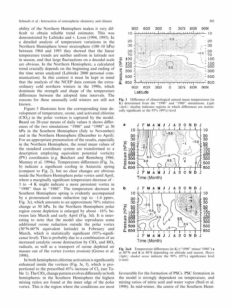
In this section the reference experiment ‘‘1990’’ (H2001)and the ‘‘1980’’ scenario run are used to analyze themodel’s ability to reproduce the temporal developmentof dynamic and chemical parameters and processesduring the most recent past. Emphasis is given tophenomena and processes relevant for stratosphericozone chemistry. Figure 1 shows the differences of thezonal and annual mean temperature between the twosimulations. Negative values indicate a cooling of theatmosphere from ‘‘1980’’ to ‘‘1990’’. Obviously, theresults demonstrate the well-known typical pattern witha warming of the troposphere and a cooling of thestratosphere due to the greenhouse effect (e.g. Rindet al. 1990; Mahfouf et al. 1994; Roeckner et al. 1999;Grewe et al. 2001). Temperature changes in polar re-gions are particularly important for stratospheric ozonedepletion and are, hence, shown in more detail inFig. 2, including the vertical and annual structure. Aunivariate statistical test (t-test) suggests that thetropospheric warming at high latitudes is not significantfor most of the time, either in the Northern Hemisphere(Fig. 2a) or in the Southern Hemisphere (Fig. 2b), ex-cept for the summer months at northern latitudes.Nevertheless, the strength of the middle tropospherictemperature changes is in agreement with observations(e.g. Steinbrecht et al. 1998; WMO 1999). Duringsouthern spring a marked cooling of the Antarcticlower stratosphere is simulated by the model (Fig. 2b).Peak values of –9 K are found at 40 hPa in November.This finding is in agreement with an analysis of Randeland Wu (1999, see their Fig. 11a) whose investigationsof the NCEP re-analysis data (1993–97 minus 1970–79)have shown a similarly strong cooling (–8 K) during thesame month. The Southern Hemisphere cooling patternin model data and observations also looks very similar:The cooling starts at higher altitudes in spring aftersunrise, and it penetrates down to lower atmosphericlayers in the following three months. However, theNCEP data show the strongest cooling around 100hPa, which is clearly below the region of maximumcooling in the model. The significantly enhanced cool-ing is linked to the strong ozone depletion in this region(not shown). Randel and Wu’s (1999) analysis showssimilarly strong temperature decreases in the NorthernHemisphere spring (their Fig. 11b), which are not re-produced by the model (Fig. 2a). Corresponding tem-perature differences calculated from E39/C data(‘‘1990’’ minus ‘‘1980’’) do not indicate a statisticallysignificant change during winter and spring. It must beemphasized that the high dynamic interannual vari-


ability of the Northern Hemisphere makes it very dif-ficult to obtain reliable trend estimates. This wasdemonstrated by Labitzke and v. Loon (1994, 1995). Ina detailed analysis of temperature variations in theNorthern Hemisphere lower stratosphere (100–10 hPa)between 1964 and 1993 they showed that the lineartemperature trends are neither uniform in latitude norin season, and that large fluctuations on a decadal scaleare obvious. In the Northern Hemisphere, a calculatedtrend crucially depends on the beginning and ending ofthe time series analyzed (Labitzke 2000 personal com-munication). In this context it must be kept in mindthat the analysis of the NCEP data contain the extra-ordinary cold northern winters in the 1990s, whichdominate the strength and shape of the temperaturedifferences between the adopted time intervals. Thereasons for these unusually cold winters are still notknown.

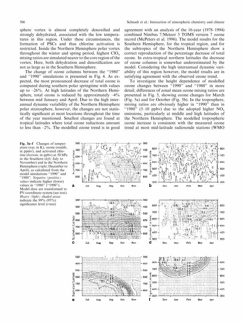
Figure 3 illustrates how the corresponding time de-velopment of temperature, ozone, and activated chlorine(ClOx) in the polar vortices is captured by the model.Based on 20-year means of daily values it shows differ-ences of the two simulations ‘‘1980’’ and ‘‘1990’’ at 50hPa in the Southern Hemisphere (July to November)and in the Northern Hemisphere (December to April).For an appropriate presentation of the results, especiallyin the Northern Hemisphere, the zonal mean values ofthe standard coordinate system are transformed to adescription employing equivalent potential vorticity(PV) coordinates (e.g. Butchart and Remsberg 1986;Manney et al. 1994a). Temperature differences (Fig. 3a,b) indicate a significant cooling in Antarctic spring(compare to Fig. 2), but no clear changes are obviousinside the Northern Hemisphere polar vortex until April,where a marginally significant temperature decrease of –3 to –4 K might indicate a more persistent vortex in‘‘1990’’ than in ‘‘1980’’. The temperature decrease inSouthern Hemisphere spring is evidently accompaniedby a pronounced ozone reduction (up to –1.4 ppmv,Fig. 3c), which amounts to an approximate 70% relativechange at 50 hPa. In the Northern Hemisphere polarregion ozone depletion is enlarged by about –16% be-tween late March and early April (Fig. 3d). It is inter-esting to note that the model also reproduces someadditional ozone reduction outside the polar vortex(30�N-60�N equivalent latitude) in February andMarch, which is statistically significant (95%-signifi-cance level). This is probably due to a combination of anincreased catalytic ozone destruction by ClOx and HOx

radicals, as well as a transport of ozone depleted airmasses out of the vortex (vortex erosion) (Grewe et al.1998).

In both hemispheres chlorine activation is significantlyenhanced inside the vortices (Fig. 3e, f), which is pro-portional to the prescribed 45% increase of Cly (see Ta-ble 1). TheClOx change pattern evolves differently in bothhemispheres: in the Southern Hemisphere the highestmixing ratios are found at the inner edge of the polarvortex. This is the region where the conditions are most

favourable for the formation of PSCs. PSC formation inthe model is strongly dependent on temperature, andmixing ratios of nitric acid and water vapor (Steil et al.1998). In mid-winter, the centre of the Southern Hemi-

Fig. 1 Difference of climatological annual mean temperatures (inK) determined from the ‘‘1990’’ and ‘‘1980’’ simulations. Light(dark) shading indicates regions in which differences are statisti-cally significant at the 95% (99%) level

Fig. 2a,b Temperature differences (in K) (‘‘1990’’ minus‘‘1980’’) aat 80�N and b at 80�S depending on altitude and season. Heavy(light) shaded areas indicate the 99% (95%) significance level(t-test)


sphere vortex is almost completely denoxified andstrongly dehydrated, associated with the low tempera-tures in this region. Under these circumstances, theformation of PSCs and thus chlorine activation isrestricted. Inside the Northern Hemisphere polar vortexthroughout the winter and spring period, highest ClOx

mixing ratios are simulated nearer to the core region of thevortex. Here, both dehydration and denoxification arenot as large as in the Southern Hemisphere.

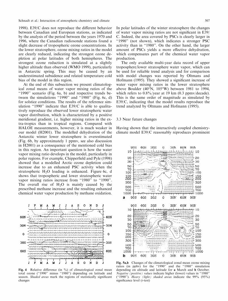
The change of ozone columns between the ‘‘1980’’and ‘‘1990’’ simulations is presented in Fig. 4. As ex-pected, the most pronounced decrease of total ozone iscomputed during southern polar springtime with valuesup to –26%. At high latitudes of the Northern Hemi-sphere, total ozone is reduced by approximately –4%between mid January and April. Due to the high inter-annual dynamic variability of the Northern Hemispherepolar stratosphere, however, the changes are not statis-tically significant at most locations throughout the timeof the year mentioned. Smallest changes are found attropical latitudes where total ozone reductions amountto less than –2%. The modelled ozone trend is in good

agreement with an analysis of the 16-year (1978–1994)combined Nimbus 7/Meteor 3 TOMS version 7 ozonerecord (McPeters et al. 1996). The model results for theSouthern Hemisphere, for the tropical region, and forthe subtropics of the Northern Hemisphere show acorrect reproduction of the percentage decrease of totalozone. In extra-tropical northern latitudes the decreaseof ozone columns is somewhat underestimated by themodel. Considering the high interannual dynamic vari-ability of this region however, the model results are insatisfying agreement with the observed ozone trend.

To investigate the height dependence of modelledozone changes between ‘‘1990’’ and ‘‘1980’’ in moredetail, differences of zonal mean ozone mixing ratios arepresented in Fig. 5, showing ozone changes for March(Fig. 5a) and for October (Fig. 5b). In the troposphere,mixing ratios are obviously higher in ‘‘1990’’ than in‘‘1980’’ (5–10 ppbv) due to the adopted higher NOx

emissions, particularly at middle and high latitudes ofthe Northern Hemisphere. The modelled troposphericozone increase is consistent with the measured ozonetrend at most mid-latitude radiosonde stations (WMO

Fig. 3a–f Changes of temper-ature (top, in K), ozone (middle,in ppmv), and activated chlo-rine (bottom, in ppbv) at 50 hPain the Southern (left; July toNovember) and in the NorthernHemisphere (right; December toApril), as calculated from themodel simulations ‘‘1990’’ and‘‘1980’’. Negative (positive)values indicate higher (lower)values in ‘‘1980’’ (‘‘1990’’).Model data are transformed toPV-coordinate system (see text).Heavy (light) shaded areasindicate the 99% (95%)significance level (t-test)


1998). E39/C does not reproduce the different behaviorbetween Canadian and European stations, as indicatedby the analysis of the period between the years 1970 and1996, where the Canadian radiosonde stations found aslight decrease of tropospheric ozone concentrations. Inthe lower stratosphere, ozone mixing ratios in the modelare clearly reduced, indicating the strongest ozone de-pletion at polar latitudes of both hemispheres. Thestrongest ozone reduction is simulated at a slightlyhigher altitude than observed (WMO 1999), particularlyin Antarctic spring. This may be caused by anunderestimated subsidence and related temperature coldbias of the model in this region.

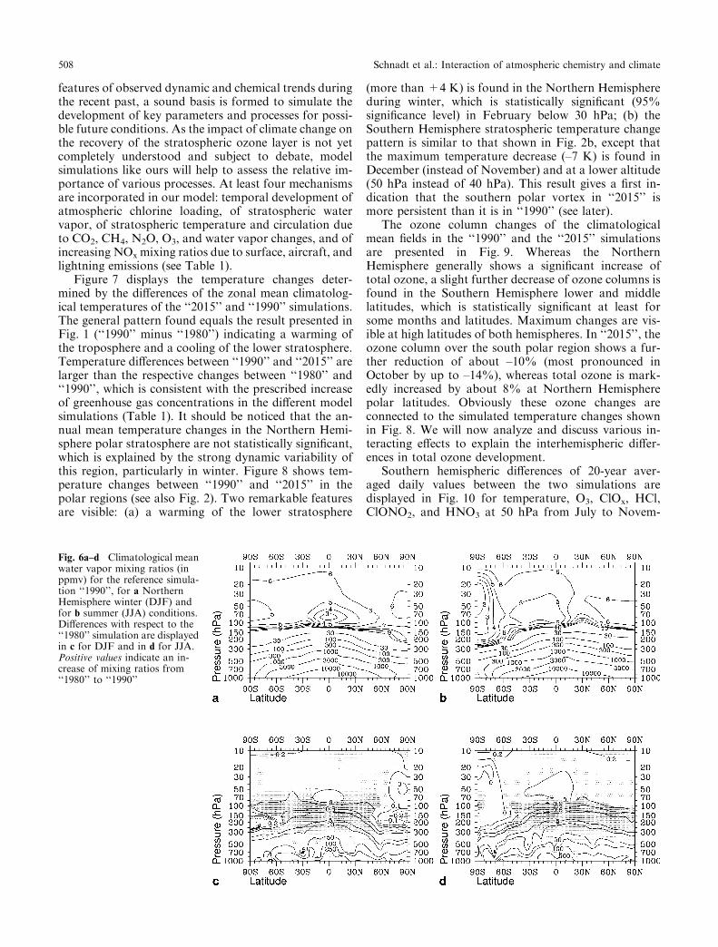
At the end of this subsection we present climatolog-ical zonal means of water vapor mixing ratios of the‘‘1990’’ scenario (Fig. 6a, b) and respective trends be-tween the simulations ‘‘1990’’ and ‘‘1980’’ (Fig. 6c, d)for solstice conditions. The results of the reference sim-ulation ‘‘1990’’ indicate that E39/C is able to qualita-tively reproduce the observed lower stratospheric watervapor distribution, which is characterized by a positivemeridional gradient, i.e. higher mixing ratios in the ex-tra-tropics than in tropical regions. Compared withHALOE measurements, however, it is much weaker inour model (H2001). The modelled dehydration of theAntarctic winter lower stratosphere is overestimated(Fig. 6b, by approximately 1 ppmv, see also discussionin H2001) as a consequence of the mentioned cold biasin this region. An important question is how the watervapor mixing ratio develops in the model, particularly inpolar regions. For example, Chipperfield and Pyle (1998)showed that a modelled Arctic ozone depletion couldincrease due to an enhanced PSC activity when thestratospheric H2O loading is enhanced. Figure 6c, dshows that tropospheric and lower stratospheric watervapor mixing ratios increase from ‘‘1980’’ to ‘‘1990’’.The overall rise of H2O is mainly caused by theprescribed methane increase and the resulting enhancedchemical water vapor production by methane oxidation.

In polar latitudes of the winter stratosphere the changesof water vapor mixing ratios are not significant in E39/C. Indeed, the area covered by PSCs is clearly larger in‘‘1990’’ (not shown), which indicates a stronger PSCactivity than in ‘‘1980’’. On the other hand, the largeramount of PSCs yields a more effective dehydration,which compensates part of the chemical water vaporproduction.

The only available multi-year data record of uppertroposphere/lower stratosphere water vapor, which canbe used for reliable trend analysis and for comparisonwith model changes was reported by Oltmans andHofmann (1995). They showed a significant increase ofwater vapor mixing ratios in the lower stratosphereabove Boulder (40�N, 105�W) between 1981 to 1994,which refers to 0.8%/year at 19 km (0.3 ppmv/decade).This is the same order of magnitude as simulated byE39/C, indicating that the model results reproduce thetrend analyzed by Oltmans and Hofmann (1995).

3.3 Near future changes

Having shown that the interactively coupled chemistry-climate model E39/C reasonably reproduces prominent

Fig. 4 Relative difference (in %) of climatological zonal meantotal ozone (‘‘1990’’ minus ‘‘1980’’) depending on latitude andseason. Shaded areas mark the regions of statistically significantchanges

Fig. 5a,b Changes of the climatological zonal mean ozone mixingratios (in ppbv) for the ‘‘1990’’ and the ‘‘1980’’ simulationdepending on altitude and latitude for a March and b October.Negative (positive) values indicate higher (lower) values in ‘‘1980’’(‘‘1990’’). Heavy (light) shaded areas indicate the 99% (95%)significance level (t-test)


features of observed dynamic and chemical trends duringthe recent past, a sound basis is formed to simulate thedevelopment of key parameters and processes for possi-ble future conditions. As the impact of climate change onthe recovery of the stratospheric ozone layer is not yetcompletely understood and subject to debate, modelsimulations like ours will help to assess the relative im-portance of various processes. At least four mechanismsare incorporated in our model: temporal development ofatmospheric chlorine loading, of stratospheric watervapor, of stratospheric temperature and circulation dueto CO2, CH4, N2O, O3, and water vapor changes, and ofincreasing NOx mixing ratios due to surface, aircraft, andlightning emissions (see Table 1).

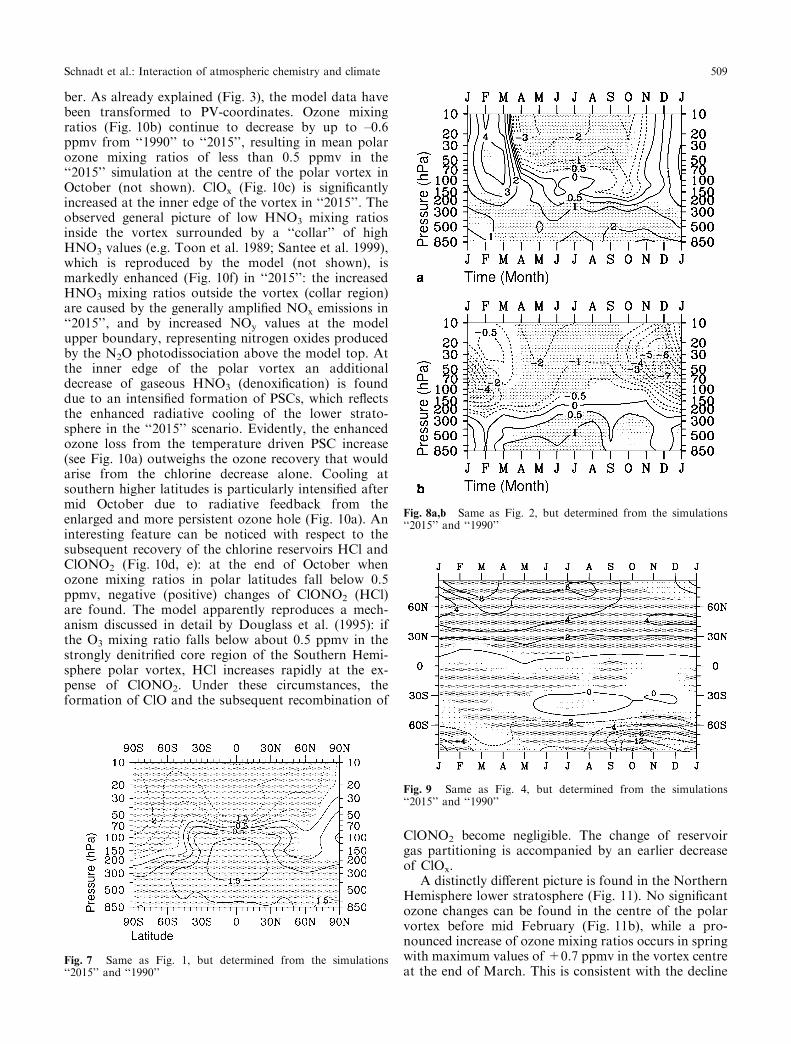
Figure 7 displays the temperature changes deter-mined by the differences of the zonal mean climatolog-ical temperatures of the ‘‘2015’’ and ‘‘1990’’ simulations.The general pattern found equals the result presented inFig. 1 (‘‘1990’’ minus ‘‘1980’’) indicating a warming ofthe troposphere and a cooling of the lower stratosphere.Temperature differences between ‘‘1990’’ and ‘‘2015’’ arelarger than the respective changes between ‘‘1980’’ and‘‘1990’’, which is consistent with the prescribed increaseof greenhouse gas concentrations in the different modelsimulations (Table 1). It should be noticed that the an-nual mean temperature changes in the Northern Hemi-sphere polar stratosphere are not statistically significant,which is explained by the strong dynamic variability ofthis region, particularly in winter. Figure 8 shows tem-perature changes between ‘‘1990’’ and ‘‘2015’’ in thepolar regions (see also Fig. 2). Two remarkable featuresare visible: (a) a warming of the lower stratosphere

(more than +4 K) is found in the Northern Hemisphereduring winter, which is statistically significant (95%significance level) in February below 30 hPa; (b) theSouthern Hemisphere stratospheric temperature changepattern is similar to that shown in Fig. 2b, except thatthe maximum temperature decrease (–7 K) is found inDecember (instead of November) and at a lower altitude(50 hPa instead of 40 hPa). This result gives a first in-dication that the southern polar vortex in ‘‘2015’’ ismore persistent than it is in ‘‘1990’’ (see later).

The ozone column changes of the climatologicalmean fields in the ‘‘1990’’ and the ‘‘2015’’ simulationsare presented in Fig. 9. Whereas the NorthernHemisphere generally shows a significant increase oftotal ozone, a slight further decrease of ozone columns isfound in the Southern Hemisphere lower and middlelatitudes, which is statistically significant at least forsome months and latitudes. Maximum changes are vis-ible at high latitudes of both hemispheres. In ‘‘2015’’, theozone column over the south polar region shows a fur-ther reduction of about –10% (most pronounced inOctober by up to –14%), whereas total ozone is mark-edly increased by about 8% at Northern Hemispherepolar latitudes. Obviously these ozone changes areconnected to the simulated temperature changes shownin Fig. 8. We will now analyze and discuss various in-teracting effects to explain the interhemispheric differ-ences in total ozone development.

Southern hemispheric differences of 20-year aver-aged daily values between the two simulations aredisplayed in Fig. 10 for temperature, O3, ClOx, HCl,ClONO2, and HNO3 at 50 hPa from July to Novem-

Fig. 6a–d Climatological meanwater vapor mixing ratios (inppmv) for the reference simula-tion ‘‘1990’’, for a NorthernHemisphere winter (DJF) andfor b summer (JJA) conditions.Differences with respect to the‘‘1980’’ simulation are displayedin c for DJF and in d for JJA.Positive values indicate an in-crease of mixing ratios from‘‘1980’’ to ‘‘1990’’


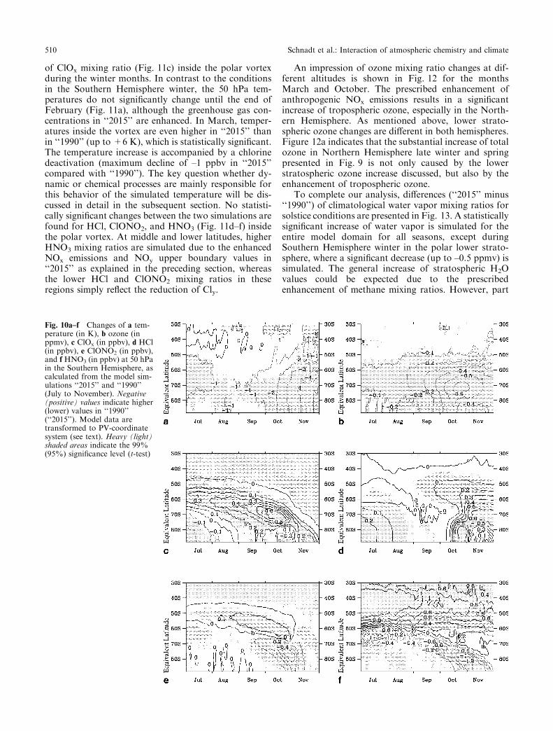
ber. As already explained (Fig. 3), the model data havebeen transformed to PV-coordinates. Ozone mixingratios (Fig. 10b) continue to decrease by up to –0.6ppmv from ‘‘1990’’ to ‘‘2015’’, resulting in mean polarozone mixing ratios of less than 0.5 ppmv in the‘‘2015’’ simulation at the centre of the polar vortex inOctober (not shown). ClOx (Fig. 10c) is significantlyincreased at the inner edge of the vortex in ‘‘2015’’. Theobserved general picture of low HNO3 mixing ratiosinside the vortex surrounded by a ‘‘collar’’ of highHNO3 values (e.g. Toon et al. 1989; Santee et al. 1999),which is reproduced by the model (not shown), ismarkedly enhanced (Fig. 10f) in ‘‘2015’’: the increasedHNO3 mixing ratios outside the vortex (collar region)are caused by the generally amplified NOx emissions in‘‘2015’’, and by increased NOy values at the modelupper boundary, representing nitrogen oxides producedby the N2O photodissociation above the model top. Atthe inner edge of the polar vortex an additionaldecrease of gaseous HNO3 (denoxification) is founddue to an intensified formation of PSCs, which reflectsthe enhanced radiative cooling of the lower strato-sphere in the ‘‘2015’’ scenario. Evidently, the enhancedozone loss from the temperature driven PSC increase(see Fig. 10a) outweighs the ozone recovery that wouldarise from the chlorine decrease alone. Cooling atsouthern higher latitudes is particularly intensified aftermid October due to radiative feedback from theenlarged and more persistent ozone hole (Fig. 10a). Aninteresting feature can be noticed with respect to thesubsequent recovery of the chlorine reservoirs HCl andClONO2 (Fig. 10d, e): at the end of October whenozone mixing ratios in polar latitudes fall below 0.5ppmv, negative (positive) changes of ClONO2 (HCl)are found. The model apparently reproduces a mech-anism discussed in detail by Douglass et al. (1995): ifthe O3 mixing ratio falls below about 0.5 ppmv in thestrongly denitrified core region of the Southern Hemi-sphere polar vortex, HCl increases rapidly at the ex-pense of ClONO2. Under these circumstances, theformation of ClO and the subsequent recombination of

ClONO2 become negligible. The change of reservoirgas partitioning is accompanied by an earlier decreaseof ClOx.

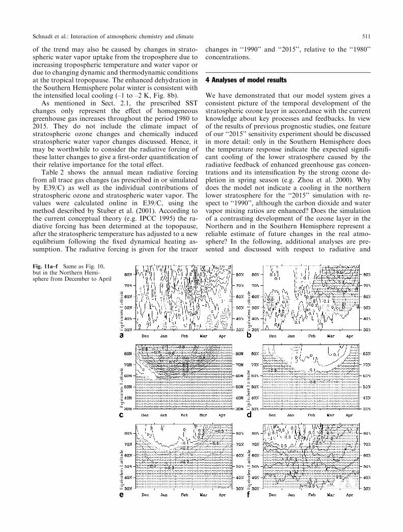
A distinctly different picture is found in the NorthernHemisphere lower stratosphere (Fig. 11). No significantozone changes can be found in the centre of the polarvortex before mid February (Fig. 11b), while a pro-nounced increase of ozone mixing ratios occurs in springwith maximum values of +0.7 ppmv in the vortex centreat the end of March. This is consistent with the decline

Fig. 8a,b Same as Fig. 2, but determined from the simulations‘‘2015’’ and ‘‘1990’’

Fig. 9 Same as Fig. 4, but determined from the simulations‘‘2015’’ and ‘‘1990’’

Fig. 7 Same as Fig. 1, but determined from the simulations‘‘2015’’ and ‘‘1990’’


of ClOx mixing ratio (Fig. 11c) inside the polar vortexduring the winter months. In contrast to the conditionsin the Southern Hemisphere winter, the 50 hPa tem-peratures do not significantly change until the end ofFebruary (Fig. 11a), although the greenhouse gas con-centrations in ‘‘2015’’ are enhanced. In March, temper-atures inside the vortex are even higher in ‘‘2015’’ thanin ‘‘1990’’ (up to +6 K), which is statistically significant.The temperature increase is accompanied by a chlorinedeactivation (maximum decline of –1 ppbv in ‘‘2015’’compared with ‘‘1990’’). The key question whether dy-namic or chemical processes are mainly responsible forthis behavior of the simulated temperature will be dis-cussed in detail in the subsequent section. No statisti-cally significant changes between the two simulations arefound for HCl, ClONO2, and HNO3 (Fig. 11d–f) insidethe polar vortex. At middle and lower latitudes, higherHNO3 mixing ratios are simulated due to the enhancedNOx emissions and NOy upper boundary values in‘‘2015’’ as explained in the preceding section, whereasthe lower HCl and ClONO2 mixing ratios in theseregions simply reflect the reduction of Cly.

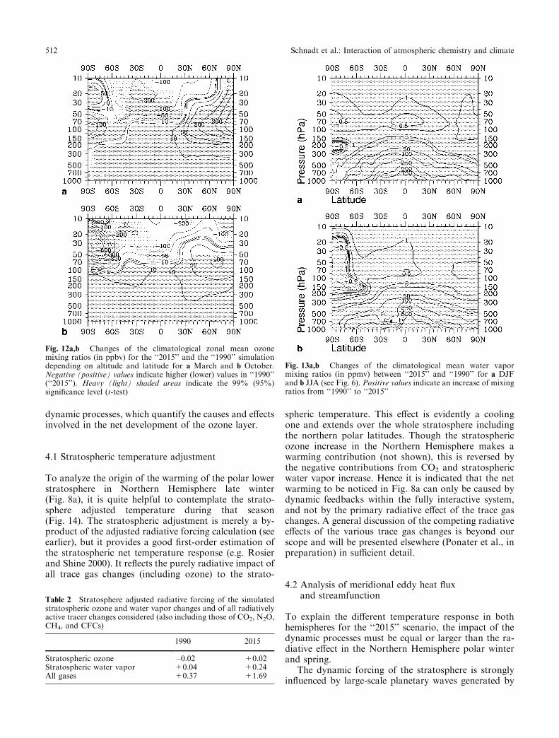
An impression of ozone mixing ratio changes at dif-ferent altitudes is shown in Fig. 12 for the monthsMarch and October. The prescribed enhancement ofanthropogenic NOx emissions results in a significantincrease of tropospheric ozone, especially in the North-ern Hemisphere. As mentioned above, lower strato-spheric ozone changes are different in both hemispheres.Figure 12a indicates that the substantial increase of totalozone in Northern Hemisphere late winter and springpresented in Fig. 9 is not only caused by the lowerstratospheric ozone increase discussed, but also by theenhancement of tropospheric ozone.

To complete our analysis, differences (‘‘2015’’ minus‘‘1990’’) of climatological water vapor mixing ratios forsolstice conditions are presented in Fig. 13. A statisticallysignificant increase of water vapor is simulated for theentire model domain for all seasons, except duringSouthern Hemisphere winter in the polar lower strato-sphere, where a significant decrease (up to –0.5 ppmv) issimulated. The general increase of stratospheric H2Ovalues could be expected due to the prescribedenhancement of methane mixing ratios. However, part

Fig. 10a–f Changes of a tem-perature (in K), b ozone (inppmv), c ClOx (in ppbv), d HCl(in ppbv), e ClONO2 (in ppbv),and f HNO3 (in ppbv) at 50 hPain the Southern Hemisphere, ascalculated from the model sim-ulations ‘‘2015’’ and ‘‘1990’’(July to November). Negative(positive) values indicate higher(lower) values in ‘‘1990’’(‘‘2015’’). Model data aretransformed to PV-coordinatesystem (see text). Heavy (light)shaded areas indicate the 99%(95%) significance level (t-test)


of the trend may also be caused by changes in strato-spheric water vapor uptake from the troposphere due toincreasing tropospheric temperature and water vapor ordue to changing dynamic and thermodynamic conditionsat the tropical tropopause. The enhanced dehydration inthe Southern Hemisphere polar winter is consistent withthe intensified local cooling (–1 to –2 K, Fig. 8b).

As mentioned in Sect. 2.1, the prescribed SSTchanges only represent the effect of homogeneousgreenhouse gas increases throughout the period 1980 to2015. They do not include the climate impact ofstratospheric ozone changes and chemically inducedstratospheric water vapor changes discussed. Hence, itmay be worthwhile to consider the radiative forcing ofthese latter changes to give a first-order quantification oftheir relative importance for the total effect.

Table 2 shows the annual mean radiative forcingfrom all trace gas changes (as prescribed in or simulatedby E39/C) as well as the individual contributions ofstratospheric ozone and stratospheric water vapor. Thevalues were calculated online in E39/C, using themethod described by Stuber et al. (2001). According tothe current conceptual theory (e.g. IPCC 1995) the ra-diative forcing has been determined at the topopause,after the stratospheric temperature has adjusted to a newequlibrium following the fixed dynamical heating as-sumption. The radiative forcing is given for the tracer

changes in ‘‘1990’’ and ‘‘2015’’, relative to the ‘‘1980’’concentrations.

4 Analyses of model results

We have demonstrated that our model system gives aconsistent picture of the temporal development of thestratospheric ozone layer in accordance with the currentknowledge about key processes and feedbacks. In viewof the results of previous prognostic studies, one featureof our ‘‘2015’’ sensitivity experiment should be discussedin more detail: only in the Southern Hemisphere doesthe temperature response indicate the expected signifi-cant cooling of the lower stratosphere caused by theradiative feedback of enhanced greenhouse gas concen-trations and its intensification by the strong ozone de-pletion in spring season (e.g. Zhou et al. 2000). Whydoes the model not indicate a cooling in the northernlower stratosphere for the ‘‘2015’’ simulation with re-spect to ‘‘1990’’, although the carbon dioxide and watervapor mixing ratios are enhanced? Does the simulationof a contrasting development of the ozone layer in theNorthern and in the Southern Hemisphere represent areliable estimate of future changes in the real atmo-sphere? In the following, additional analyses are pre-sented and discussed with respect to radiative and

Fig. 11a–f Same as Fig. 10,but in the Northern Hemi-sphere from December to April


dynamic processes, which quantify the causes and effectsinvolved in the net development of the ozone layer.

4.1 Stratospheric temperature adjustment

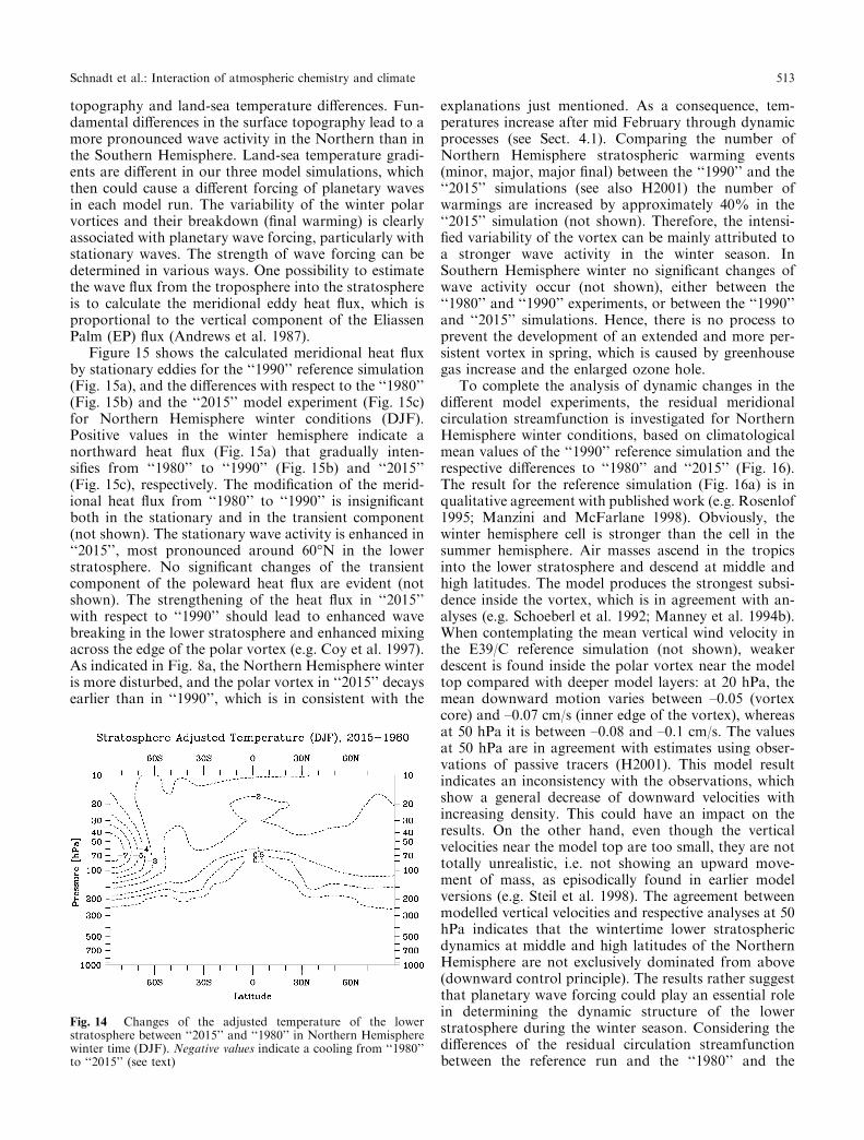
To analyze the origin of the warming of the polar lowerstratosphere in Northern Hemisphere late winter(Fig. 8a), it is quite helpful to contemplate the strato-sphere adjusted temperature during that season(Fig. 14). The stratospheric adjustment is merely a by-product of the adjusted radiative forcing calculation (seeearlier), but it provides a good first-order estimation ofthe stratospheric net temperature response (e.g. Rosierand Shine 2000). It reflects the purely radiative impact ofall trace gas changes (including ozone) to the strato-

spheric temperature. This effect is evidently a coolingone and extends over the whole stratosphere includingthe northern polar latitudes. Though the stratosphericozone increase in the Northern Hemisphere makes awarming contribution (not shown), this is reversed bythe negative contributions from CO2 and stratosphericwater vapor increase. Hence it is indicated that the netwarming to be noticed in Fig. 8a can only be caused bydynamic feedbacks within the fully interactive system,and not by the primary radiative effect of the trace gaschanges. A general discussion of the competing radiativeeffects of the various trace gas changes is beyond ourscope and will be presented elsewhere (Ponater et al., inpreparation) in sufficient detail.

4.2 Analysis of meridional eddy heat fluxand streamfunction

To explain the different temperature response in bothhemispheres for the ‘‘2015’’ scenario, the impact of thedynamic processes must be equal or larger than the ra-diative effect in the Northern Hemisphere polar winterand spring.

The dynamic forcing of the stratosphere is stronglyinfluenced by large-scale planetary waves generated by

Fig. 12a,b Changes of the climatological zonal mean ozonemixing ratios (in ppbv) for the ‘‘2015’’ and the ‘‘1990’’ simulationdepending on altitude and latitude for a March and b October.Negative (positive) values indicate higher (lower) values in ‘‘1990’’(‘‘2015’’). Heavy (light) shaded areas indicate the 99% (95%)significance level (t-test)

Fig. 13a,b Changes of the climatological mean water vapormixing ratios (in ppmv) between ‘‘2015’’ and ‘‘1990’’ for a DJFand b JJA (see Fig. 6). Positive values indicate an increase of mixingratios from ‘‘1990’’ to ‘‘2015’’

Table 2 Stratosphere adjusted radiative forcing of the simulatedstratospheric ozone and water vapor changes and of all radiativelyactive tracer changes considered (also including those of CO2, N2O,CH4, and CFCs)

1990 2015

Stratospheric ozone –0.02 +0.02Stratospheric water vapor +0.04 +0.24All gases +0.37 +1.69


topography and land-sea temperature differences. Fun-damental differences in the surface topography lead to amore pronounced wave activity in the Northern than inthe Southern Hemisphere. Land-sea temperature gradi-ents are different in our three model simulations, whichthen could cause a different forcing of planetary wavesin each model run. The variability of the winter polarvortices and their breakdown (final warming) is clearlyassociated with planetary wave forcing, particularly withstationary waves. The strength of wave forcing can bedetermined in various ways. One possibility to estimatethe wave flux from the troposphere into the stratosphereis to calculate the meridional eddy heat flux, which isproportional to the vertical component of the EliassenPalm (EP) flux (Andrews et al. 1987).

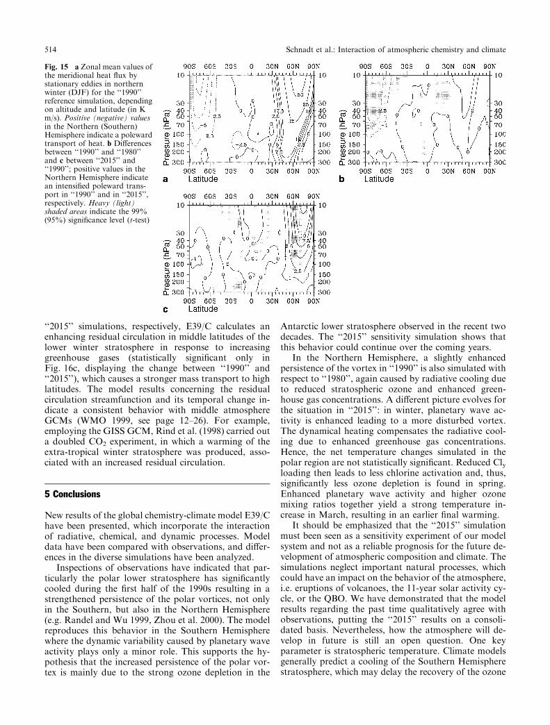
Figure 15 shows the calculated meridional heat fluxby stationary eddies for the ‘‘1990’’ reference simulation(Fig. 15a), and the differences with respect to the ‘‘1980’’(Fig. 15b) and the ‘‘2015’’ model experiment (Fig. 15c)for Northern Hemisphere winter conditions (DJF).Positive values in the winter hemisphere indicate anorthward heat flux (Fig. 15a) that gradually inten-sifies from ‘‘1980’’ to ‘‘1990’’ (Fig. 15b) and ‘‘2015’’(Fig. 15c), respectively. The modification of the merid-ional heat flux from ‘‘1980’’ to ‘‘1990’’ is insignificantboth in the stationary and in the transient component(not shown). The stationary wave activity is enhanced in‘‘2015’’, most pronounced around 60�N in the lowerstratosphere. No significant changes of the transientcomponent of the poleward heat flux are evident (notshown). The strengthening of the heat flux in ‘‘2015’’with respect to ‘‘1990’’ should lead to enhanced wavebreaking in the lower stratosphere and enhanced mixingacross the edge of the polar vortex (e.g. Coy et al. 1997).As indicated in Fig. 8a, the Northern Hemisphere winteris more disturbed, and the polar vortex in ‘‘2015’’ decaysearlier than in ‘‘1990’’, which is in consistent with the

explanations just mentioned. As a consequence, tem-peratures increase after mid February through dynamicprocesses (see Sect. 4.1). Comparing the number ofNorthern Hemisphere stratospheric warming events(minor, major, major final) between the ‘‘1990’’ and the‘‘2015’’ simulations (see also H2001) the number ofwarmings are increased by approximately 40% in the‘‘2015’’ simulation (not shown). Therefore, the intensi-fied variability of the vortex can be mainly attributed toa stronger wave activity in the winter season. InSouthern Hemisphere winter no significant changes ofwave activity occur (not shown), either between the‘‘1980’’ and ‘‘1990’’ experiments, or between the ‘‘1990’’and ‘‘2015’’ simulations. Hence, there is no process toprevent the development of an extended and more per-sistent vortex in spring, which is caused by greenhousegas increase and the enlarged ozone hole.

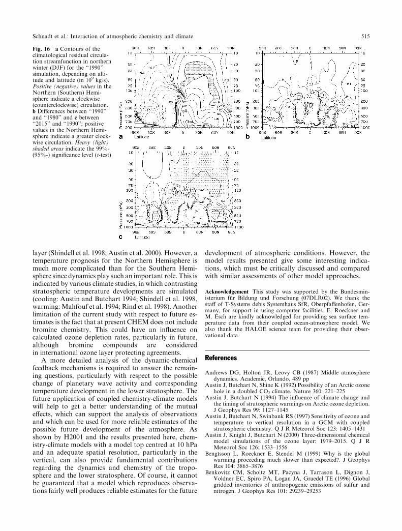
To complete the analysis of dynamic changes in thedifferent model experiments, the residual meridionalcirculation streamfunction is investigated for NorthernHemisphere winter conditions, based on climatologicalmean values of the ‘‘1990’’ reference simulation and therespective differences to ‘‘1980’’ and ‘‘2015’’ (Fig. 16).The result for the reference simulation (Fig. 16a) is inqualitative agreement with published work (e.g. Rosenlof1995; Manzini and McFarlane 1998). Obviously, thewinter hemisphere cell is stronger than the cell in thesummer hemisphere. Air masses ascend in the tropicsinto the lower stratosphere and descend at middle andhigh latitudes. The model produces the strongest subsi-dence inside the vortex, which is in agreement with an-alyses (e.g. Schoeberl et al. 1992; Manney et al. 1994b).When contemplating the mean vertical wind velocity inthe E39/C reference simulation (not shown), weakerdescent is found inside the polar vortex near the modeltop compared with deeper model layers: at 20 hPa, themean downward motion varies between –0.05 (vortexcore) and –0.07 cm/s (inner edge of the vortex), whereasat 50 hPa it is between –0.08 and –0.1 cm/s. The valuesat 50 hPa are in agreement with estimates using obser-vations of passive tracers (H2001). This model resultindicates an inconsistency with the observations, whichshow a general decrease of downward velocities withincreasing density. This could have an impact on theresults. On the other hand, even though the verticalvelocities near the model top are too small, they are nottotally unrealistic, i.e. not showing an upward move-ment of mass, as episodically found in earlier modelversions (e.g. Steil et al. 1998). The agreement betweenmodelled vertical velocities and respective analyses at 50hPa indicates that the wintertime lower stratosphericdynamics at middle and high latitudes of the NorthernHemisphere are not exclusively dominated from above(downward control principle). The results rather suggestthat planetary wave forcing could play an essential rolein determining the dynamic structure of the lowerstratosphere during the winter season. Considering thedifferences of the residual circulation streamfunctionbetween the reference run and the ‘‘1980’’ and the

Fig. 14 Changes of the adjusted temperature of the lowerstratosphere between ‘‘2015’’ and ‘‘1980’’ in Northern Hemispherewinter time (DJF). Negative values indicate a cooling from ‘‘1980’’to ‘‘2015’’ (see text)


‘‘2015’’ simulations, respectively, E39/C calculates anenhancing residual circulation in middle latitudes of thelower winter stratosphere in response to increasinggreenhouse gases (statistically significant only inFig. 16c, displaying the change between ‘‘1990’’ and‘‘2015’’), which causes a stronger mass transport to highlatitudes. The model results concerning the residualcirculation streamfunction and its temporal change in-dicate a consistent behavior with middle atmosphereGCMs (WMO 1999, see page 12–26). For example,employing the GISS GCM, Rind et al. (1998) carried outa doubled CO2 experiment, in which a warming of theextra-tropical winter stratosphere was produced, asso-ciated with an increased residual circulation.

5 Conclusions

New results of the global chemistry-climate model E39/Chave been presented, which incorporate the interactionof radiative, chemical, and dynamic processes. Modeldata have been compared with observations, and differ-ences in the diverse simulations have been analyzed.

Inspections of observations have indicated that par-ticularly the polar lower stratosphere has significantlycooled during the first half of the 1990s resulting in astrengthened persistence of the polar vortices, not onlyin the Southern, but also in the Northern Hemisphere(e.g. Randel and Wu 1999, Zhou et al. 2000). The modelreproduces this behavior in the Southern Hemispherewhere the dynamic variability caused by planetary waveactivity plays only a minor role. This supports the hy-pothesis that the increased persistence of the polar vor-tex is mainly due to the strong ozone depletion in the

Antarctic lower stratosphere observed in the recent twodecades. The ‘‘2015’’ sensitivity simulation shows thatthis behavior could continue over the coming years.

In the Northern Hemisphere, a slightly enhancedpersistence of the vortex in ‘‘1990’’ is also simulated withrespect to ‘‘1980’’, again caused by radiative cooling dueto reduced stratospheric ozone and enhanced green-house gas concentrations. A different picture evolves forthe situation in ‘‘2015’’: in winter, planetary wave ac-tivity is enhanced leading to a more disturbed vortex.The dynamical heating compensates the radiative cool-ing due to enhanced greenhouse gas concentrations.Hence, the net temperature changes simulated in thepolar region are not statistically significant. Reduced Clyloading then leads to less chlorine activation and, thus,significantly less ozone depletion is found in spring.Enhanced planetary wave activity and higher ozonemixing ratios together yield a strong temperature in-crease in March, resulting in an earlier final warming.

It should be emphasized that the ‘‘2015’’ simulationmust been seen as a sensitivity experiment of our modelsystem and not as a reliable prognosis for the future de-velopment of atmospheric composition and climate. Thesimulations neglect important natural processes, whichcould have an impact on the behavior of the atmosphere,i.e. eruptions of volcanoes, the 11-year solar activity cy-cle, or the QBO. We have demonstrated that the modelresults regarding the past time qualitatively agree withobservations, putting the ‘‘2015’’ results on a consoli-dated basis. Nevertheless, how the atmosphere will de-velop in future is still an open question. One keyparameter is stratospheric temperature. Climate modelsgenerally predict a cooling of the Southern Hemispherestratosphere, which may delay the recovery of the ozone

Fig. 15 a Zonal mean values ofthe meridional heat flux bystationary eddies in northernwinter (DJF) for the ‘‘1990’’reference simulation, dependingon altitude and latitude (in Km/s). Positive (negative) valuesin the Northern (Southern)Hemisphere indicate a polewardtransport of heat. b Differencesbetween ‘‘1990’’ and ‘‘1980’’and c between ‘‘2015’’ and‘‘1990’’; positive values in theNorthern Hemisphere indicatean intensified poleward trans-port in ‘‘1990’’ and in ‘‘2015’’,respectively. Heavy (light)shaded areas indicate the 99%(95%) significance level (t-test)


layer (Shindell et al. 1998; Austin et al. 2000). However, atemperature prognosis for the Northern Hemisphere ismuch more complicated than for the Southern Hemi-sphere since dynamics play such an important role. This isindicated by various climate studies, in which contrastingstratospheric temperature developments are simulated(cooling: Austin and Butchart 1994; Shindell et al. 1998,warming: Mahfouf et al. 1994; Rind et al. 1998). Anotherlimitation of the current study with respect to future es-timates is the fact that at present CHEM does not includebromine chemistry. This could have an influence oncalculated ozone depletion rates, particularly in future,although bromine compounds are consideredin international ozone layer protecting agreements.

A more detailed analysis of the dynamic-chemicalfeedback mechanisms is required to answer the remain-ing questions, particularly with respect to the possiblechange of planetary wave activity and correspondingtemperature development in the lower stratosphere. Thefuture application of coupled chemistry-climate modelswill help to get a better understanding of the mutualeffects, which can support the analysis of observationsand which can be used for more reliable estimates of thepossible future development of the atmosphere. Asshown by H2001 and the results presented here, chem-istry-climate models with a model top centred at 10 hPaand an adequate spatial resolution, particularly in thevertical, can also provide fundamental contributionsregarding the dynamics and chemistry of the tropo-sphere and the lower stratosphere. Of course, it cannotbe guaranteed that a model which reproduces observa-tions fairly well produces reliable estimates for the future

development of atmospheric conditions. However, themodel results presented give some interesting indica-tions, which must be critically discussed and comparedwith similar assessments of other model approaches.

Acknowledgement This study was supported by the Bundesmin-isterium fur Bildung und Forschung (07DLR02). We thank thestaff of T-Systems debis Systemhaus SfR, Oberpfaffenhofen, Ger-many, for support in using computer facilities. E. Roeckner andM. Esch are kindly acknowledged for providing sea surface tem-perature data from their coupled ocean-atmosphere model. Wealso thank the HALOE science team for providing their obser-vational data.

References

Andrews DG, Holton JR, Leovy CB (1987) Middle atmospheredynamics. Academic, Orlando, 489 pp

Austin J, Butchart N, Shine K (1992) Possibility of an Arctic ozonehole in a doubled CO2 climate. Nature 360: 221–225

Austin J, Butchart N (1994) The influence of climate change andthe timing of stratospheric warmings on Arctic ozone depletion.J Geophys Res 99: 1127–1145

Austin J, Butchart N, Swinbank RS (1997) Sensitivity of ozone andtemperature to vertical resolution in a GCM with coupledstratospheric chemistry. Q J R Meteorol Soc 123: 1405–1431

Austin J, Knight J, Butchart N (2000) Three-dimensional chemicalmodel simulations of the ozone layer: 1979–2015. Q J RMeteorol Soc 126: 1533–1556

Bengtsson L, Roeckner E, Stendel M (1999) Why is the globalwarming proceeding much slower than expected?. J GeophysRes 104: 3865–3876

Benkovitz CM, Scholtz MT, Pacyna J, Tarrason L, Dignon J,Voldner EC, Spiro PA, Logan JA, Graedel TE (1996) Globalgridded inventories of anthropogenic emissions of sulfur andnitrogen. J Geophys Res 101: 29239–29253

Fig. 16 a Contours of theclimatological residual circula-tion streamfunction in northernwinter (DJF) for the ‘‘1990’’simulation, depending on alti-tude and latitude (in 109 kg/s).Positive (negative) values in theNorthern (Southern) Hemi-sphere indicate a clockwise(counterclockwise) circulation.b Differences between ‘‘1990’’and ‘‘1980’’ and c between‘‘2015’’ and ‘‘1990’’; positivevalues in the Northern Hemi-sphere indicate a greater clock-wise circulation. Heavy (light)shaded areas indicate the 99%-(95%-) significance level (t-test)


Boughner RE (1978) The effect of increased carbon dioxide con-centrations on stratospheric ozone. J Geophys Res 83: 1326–1332

Bruhl C, Crutzen PJ (1993) MPIC two-dimensional model. NASARef Publ 1292: 103–104

Butchart N, Remsberg EE (1986) The area of the stratosphericpolar vortex as a diagnostic for tracer transport on an isen-tropic surface. J Atmos Sci 43: 1319–1339

Cariolle D, Lasserre-Bigorry A, Royer J-F, Geleyn J-F (1990) AGCM simulation of the springtime Antarctic ozone decreaseand its impact on mid-latitudes. J Geophys Res 95: 1883–1898

Chipperfield MP, Pyle JA (1998) Model sensitivity studies of arcticozone depletion. J Geophys Res 103: 28389–28403

Coy L, Nash ER, Newman PA (1997) Meteorology of the polarvortex: spring 1997. Geophys Res Lett 24: 2693–2696

Dameris M, Berger U, Gunther G, Ebel A (1991) The ozone hole:dynamical consequences as simulated with a three-dimensionalmodel of the middle atmosphere. Ann Geophys 9: 661–668

Dameris M, Grewe V, Hein R, Schnadt C, Bruhl C, Steil B (1998)Assessment of the future development of the ozone layer.Geophys Res Lett 25: 3579–3582

Danilin MY, Sze N-D, Ko MKW, Rodriguez JM, Tabazadeh A(1998) Stratospheric cooling and Arctic ozone recovery. Geo-phys Res Lett 25: 2141–2144

Douglass AR, Schoeberl MR, Stolarski RS, Waters JW, Russell IIIJM, Roche AE, Massie ST (1995) Inter-hemispheric differencesin springtime production of HCl and ClONO2 in the polarvortices. J Geophys Res 100: 13967–13978

Fels SB, Mahlmann JD, Schwarzkopf MD, Sinclair RW (1980)Stratospheric sensitivity to perturbations in ozone and carbondioxide: radiative and dynamical response. J Atmos Sci 37:2265–2297

Forster PM de F (1999) Radiative forcing due to stratosphericozone changes 1979–1997, using updated trend estimates.J Geophys Res 104: 24 395–24399

Gates WL (1992) AMIP: the atmosphere model inter-comparisonproject. Bull Am Meteorol Soc 73: 1962–1970

Graf H-F, Kirchner I, Perlwitz J (1998) Changing lower strato-spheric circulation: the role of ozone and greenhouse gases.J Geophys Res 103: 11251–11261

Grewe V, Dameris M, Sausen R, Steil B (1998) Impact of strato-spheric dynamics and chemistry on northern hemisphere mid-latitude ozone loss. J Geophys Res 103: 25417–25433

Grewe V, Dameris M, Hein R, Sausen R, Steil B (2001) Futurechanges of the atmospheric composition and the impact ofclimate change. Tellus 53B: 103–121

Groves KS, Mattingly SR, Tuck AF (1978) Increased atmosphericcarbon dioxide and stratospheric ozone. Nature 273: 711–715

Hartmann DL, Wallace JM, Limpasuvan V, Thomson DWJ,Holton JR (2000) Can ozone depletion and global warminginteract to produce rapid climate change? PNAS 97: 1412–1417

Hein R, Dameris M, Schnadt C, Land C, Grewe V, Kohler I,PonaterM, SausenR, Steil B, Landgraf J, Bruhl C (2001) Resultsof an interactively coupled chemistry-general circulation model:comparison with observations. Ann Geophys 19: 435–457

Huntrieser H, Schlager H, Feigl C, Holler H (1998) The transportand production of NOx in electrified thunderstorms: survey ofprevious studies and new observations at mid-latitudes.J Geophys Res 103: 28247–28264

IPCC (1990) (Intergovernmental Panel on Climate Change) Cli-mate change, The IPCC Scientific Assessment. Houghton JTet al. (eds) Cambridge University Press, Cambridge

IPCC (1995) (Intergovernmental Panel on Climate Change) Cli-mate change 1994, Radiative forcing of climate change.Houghton JT et al. (eds) Cambridge University Press, Cam-bridge

IPCC (1996) (Intergovernmental Panel on Climate Change) Cli-mate change 1995, The science of climate change. Houghton JTet al. (eds) Cambridge University Press, Cambridge

IPCC (1999) (Intergovernmental Panel on Climate Change) Avia-tion and the global atmosphere. Penner JE, Lister DH, Griggs

DJ, Dokken DJ, McFarland M (eds) Cambridge UniversityPress, Cambridge

Kivi R, Kyro E, Turunen T, Ulich T, Turunen E (1999) Atmo-spheric trends above Finland: II. Troposphere and stratosphere.Geophysica 35: 71–85

Labitzke K, van Loon H (1994) Trends of temperature and geo-potential height between 100 and 10 hPa in the northernhemisphere. J Meteorol Soc Japan 72: 643–652

Labitzke K, van Loon H (1995) A note on the distribution oftrends below 10 hPa: the extra-tropical northern hemisphere.J Meteorol Soc Jpn 73: 883–889

Land C, Ponater M, Sausen R, Roeckner E (1999) TheECHAM4.L39(DLR) atmosphere GCM – Technical descrip-tion and model climatology. DLR-Oberpfaffenhofen, Rep1991–31, Wessling, Germany, ISSN 1434–8454

Langematz U (2000) An estimate of the impact of observed ozonelosses on stratospheric temperature. Geophys Res Lett 27:2077–2080

Mahfouf JF, Cariolle D, Royer J-F, Geleyn J-F, Timbal B (1994)Response of the meteo-France climate model to changes in CO2

and the sea surface temperature. Clim Dyn 9: 345–362Manney GL, Zurek RW, Gelman ME, Miller AJ, Nagatani R

(1994a) The anomalous Arctic lower stratospheric polar vortex.Geophys Res Lett 21: 2405–2408

Manney GL, Zurek RW, O’Neill A, Swinbank R (1994b) On themotion of air through the stratospheric polar vortex. J AtmosSci 51: 2973–2994

Manzini E, McFarlane NA (1998) The effect of varying the sourcespectrum of a gravity wave parameterization in a middle at-mosphere general circulation model. J Geophys Res 103:31523–31539

McPeters RD, Hollandsworth SM, Flynn LE, Herman JR, SeftorCJ (1996) Long-term ozone trends derived from the 16-yearcombined Nimbus 7/Meteor 3 TOMS version 7 record. Geo-phys Res Lett 23: 3699–3702

Montzka SA, Butler JH, Myers RC, Thompson TM, Swanson TH,Clarke AD, Lock LT, Elkins JW (1996) Decline in the tropo-spheric abundance of halogen from halocarbons: implicationsfor stratospheric ozone depletion. Science 272: 1318–1322

Montzka SA, Butler JH, Elkins JW, Thompson TM, Clarke AD,Lock LT (1999) Present and future trends in the atmosphericburden of ozone-depleting halogens. Nature 398: 690–694

Oltmans SJ, Hofmann DJ (1995) Increase in lower stratosphericwater vapor at mid-latitude northern hemisphere site from 1981to 1994. Nature 374: 146–149

Pawson S, Labitzke K, Leder S (1998) Stepwise changes instratospheric temperatures. Geophys Res Lett 25: 2157–2160

Pawson S et al. (2000) The GCM-reality inter-comparison projectof SPARC (GRIPS): scientific issues and initial results. Bull AmMeteorol Soc 81: 781–796

Perlwitz J, Graf H-F (1995) The statistical connection betweentropospheric and stratospheric circulation of the northernhemisphere in winter. J Clim 8: 2281–2295

Perlwitz J, Graf H-F, Voss R (2000) The leading mode of thecoupled troposphere-stratosphere winter circulation in differentclimate regimes. J Geophys Res 105: 6915–6926

Pitari G, Palermi S, Visconti G (1992) Ozone response to a CO2

doubling: results from a stratospheric circulation model withheterogeneous chemistry. J Geophys Res 97: 5953–5962

Price C, Rind D (1992) A simple lightning parameterization forcalculating global lightning distributions. J Geophys Res 97:9919–9933

Price C, Rind D (1994) Modeling global lightning distributions in ageneral circulation model. Mon Weather Rev 122: 1930–1937

Ramanathan V, Callis LB, Boughner RE (1976) Sensitivity ofsurface temperature and atmospheric temperature to pertur-bations in the stratospheric concentration of ozone and nitro-gen dioxide. J Atmos Sci 33: 1092–1112

Randel WJ, Wu F (1999) Cooling of the Arctic and Antarctic polarstratosphere due to ozone depletion. J Clim 12: 1467–1479


Rind D, Suozzo R, Balachandran NK, Prather MJ (1990) Climatechange and the middle atmosphere. Part I: the doubled CO2

climate. J Atmos Sci 47: 475–494Rind D, Shindell D, Lonergan P, Balachandran NK (1998) Climate

change and the middle atmosphere: Part III, The doubled CO2

climate revisited. J Clim 11: 876–894Roeckner E, Bengtsson L, Feichter J, Leliefeld J, Rodhe H (1999)

Transient climate change simulations with a coupled atmo-sphere-ocean GCM including the tropospheric sulfur cycle.J Clim 12: 3003–3032

Rosenlof KH (1995) Seasonal cycle of the residual mean meridionalcirculation in the stratosphere. J Geophys Res 100: 5173–5191

Rosier SM, KP Shine (2000) The effect of two decades of ozonechanges on stratospheric temperature as indicated by a generalcirculation model. Geophys Res Lett 27: 2617–2620

Santee ML, Manney GL, Froidevaux L, Read WG, Waters JW(1999) Six years of UARS Microwave Limb Sounder HNO3

observations: seasonal, inter-hemispheric, and inter-annualvariations in the lower stratosphere. J Geophys Res 104: 8225–8246

Santer BD, Hnilo JJ, Wigley TML, Boyle JS, Doutriaux C, FiorinoM, Parker DE, Taylor KE (1999) Uncertainties in observa-tionally based estimates of temperature changes in the freeatmosphere. J Geophys Res 104: 6305–6333

Schmitt A, Brunner B (1997) Emissions from aviation and theirdevelopment over time. In: Schumann U. et al. (ed) Pollutantsfrom air traffic – results from atmospheric research 1992–1997,DLR-Mitteilungen, 97–04, DLR-Koln, Germany, pp 37–52

Schoeberl MR, Lait LR, Newman PA, Rosenfield JE (1992) Thestructure of the polar vortex. J Geophys Res 97: 7859–7882

Shindell DT, Rind D, Lonergan P (1998) Increased polar strato-spheric ozone losses and delayed eventual recovery owing toincreasing greenhouse-gas concentrations. Nature 392:589–592

Shine KP (1986) On the modelled thermal response of the Antarcticstratosphere to a depletion of ozone. Geophys Res Lett 13:1331–1334

Shine KP (1989) Sources and sinks of zonal momentum in themiddle atmosphere using the diabatic circulation. Q J RMeteorol Soc 115: 265–292

Steil B, Dameris M, Bruhl C, Crutzen PJ, Grewe V, Ponater M,Sausen R (1998) Development of a chemistry module forGCMs: first results of a multi-annual integration. Ann Geophys16: 205–228

Steinbrecht W, Claude H, Kohler U, Hoinka KP (1998) Corre-lations between tropopause height and total ozone: implica-tions for long-term changes. J Geophys Res 103: 19183–19192

Stuber N, Sausen R, Ponater M (2001) Stratosphere adjusted ra-diative forcing calculations in a comprehensive climate model.Theor Appl Climatol 68: 125–135

Timmreck C, Graf H-F, Feichter J (1999) Simulation of Mt.Pinatubo volcanic aerosol with the Hamburg climate modelECHAM4. Theor Appl Climatol 62: 85–108

Toon GC, Farmer CB, Lowes LL, Schaper PW, Blavier J-F,Norton RH (1989) Infrared aircraft measurements of strato-spheric composition over Antarctica during September 1987.J Geophys Res 94: 16571–16596

WMO (1998) (World Meteorological Organisation) Assessment oftrends in the vertical distribution of ozone. SPARC Report 1,Ozone Research and Monitoring Project, Report 43

WMO (1999) (World Meteorological Organisation) Scientific as-sessment of ozone depletion: 1998. Global Ozone Research andMonitoring Project, Report 44

Zhou S, Gelman ME, Miller AJ, McCormack JP (2000) An inter-hemispheric comparison of the persistent stratospheric polarvortex. Geophys Res Lett 27: 1123–1126


interaction of atmospheric chemistry and climate and its impact on stratospheric ozone

Documents