integrating hydrogeodetic data and models: towards an assimilative framework jürgen kusche, annette...
TRANSCRIPT
Integrating hydrogeodetic data and models: towards an assimilative
framework
Jürgen Kusche, Annette Eicker, Maike SchumacherBonn University
With input from Petra Döll, Hannes Müller-Schmied (Frankfurt University)
IGCP Workshop, October 29/30, 2012, Johannesburg 1
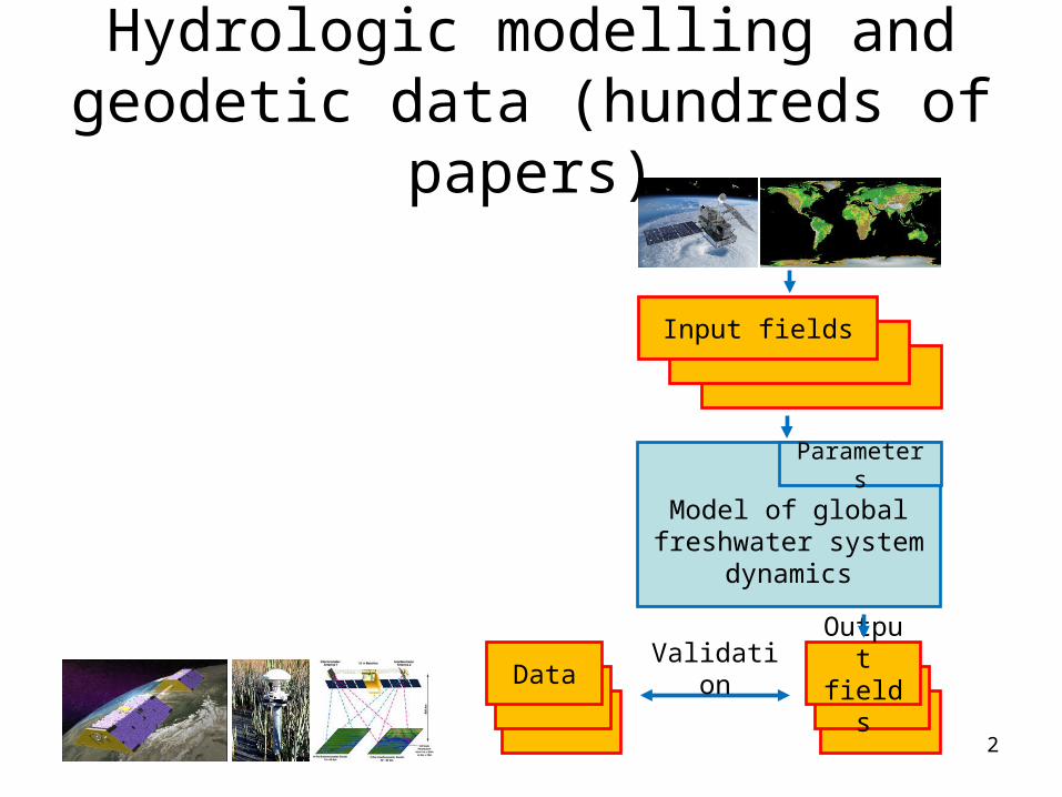
Hydrologic modelling and geodetic data (hundreds of papers)
Model of global freshwater system
dynamics
Input fields
Parameters
Validation Output fields
Data
2

What we now should do
Model of global freshwater system
dynamics
Output fields
Input fields
Parameters
Calibration Data
Assimilation3

Challenges
Model of global freshwater system
dynamics
Output fields
Scenario inputs
Parameters
Climate model scenario
DataNew sensors
New sensors
• Understanding the present state of the global freshwater system– Freshwater as a ressource– Memory function for climate– Being able to reliably
simulate future evolution
• Challenges– Global scale: data problem– Limited representation of
physics / conceptual realism in the models
– Being able to assess the potential of new and future sensors, data sets, models
4
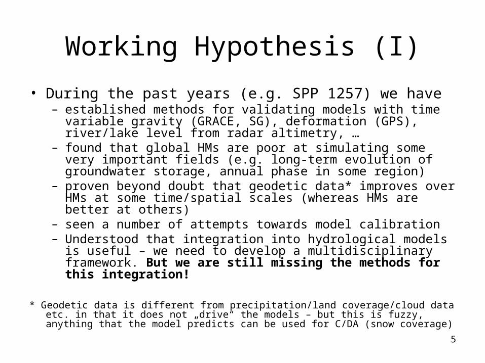
Working Hypothesis (I)
• During the past years (e.g. SPP 1257) we have– established methods for validating models with time variable
gravity (GRACE, SG), deformation (GPS), river/lake level from radar altimetry, …
– found that global HMs are poor at simulating some very important fields (e.g. long-term evolution of groundwater storage, annual phase in some region)
– proven beyond doubt that geodetic data* improves over HMs at some time/spatial scales (whereas HMs are better at others)
– seen a number of attempts towards model calibration– Understood that integration into hydrological models is useful –
we need to develop a multidisciplinary framework. But we are still missing the methods for this integration!
* Geodetic data is different from precipitation/land coverage/cloud data etc. in that it does not „drive“ the models – but this is fuzzy, anything that the model predicts can be used for C/DA (snow coverage)
5
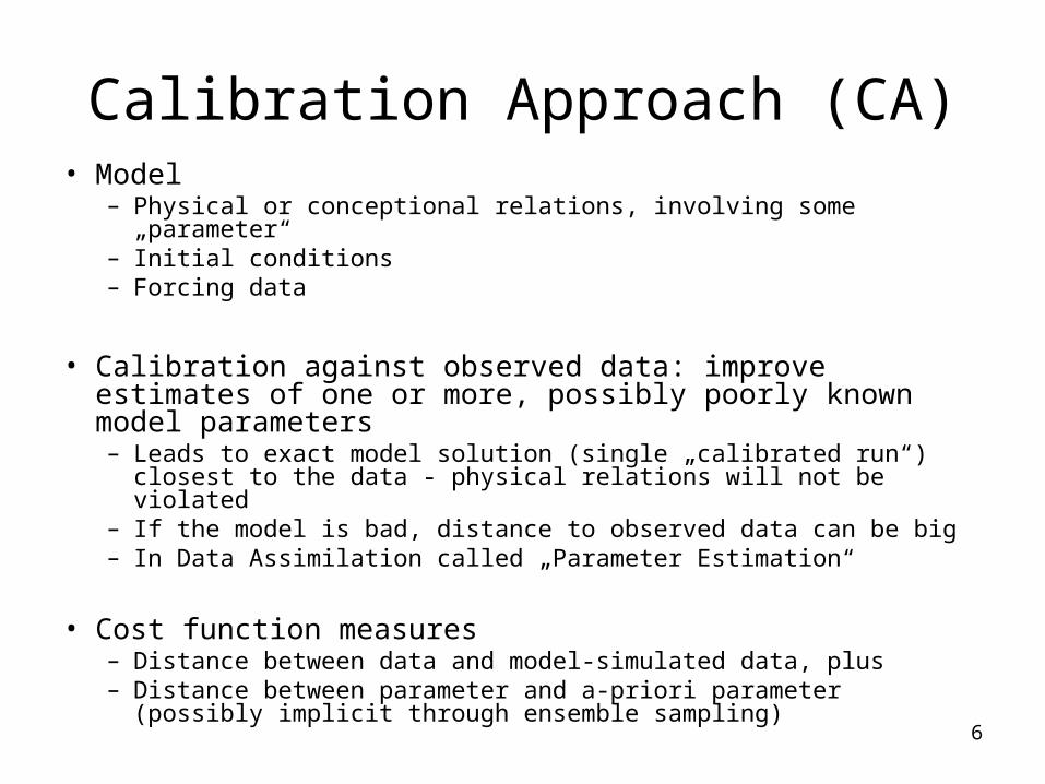
Calibration Approach (CA)• Model
– Physical or conceptional relations, involving some „parameter“– Initial conditions– Forcing data
• Calibration against observed data: improve estimates of one or more, possibly poorly known model parameters– Leads to exact model solution (single „calibrated run“) closest to
the data - physical relations will not be violated– If the model is bad, distance to observed data can be big– In Data Assimilation called „Parameter Estimation“
• Cost function measures– Distance between data and model-simulated data, plus– Distance between parameter and a-priori parameter (possibly
implicit through ensemble sampling) 6

Werth and Güntner (2009, 2010)
• WGHM with ECMWF/GPCC forcing• Select 6-8 most relevant parameters per basin (based on
sensitivity analysis / MC simulation)• Calibration data: GRACE TWS basin average + monthly
mean runoff• Cost function with 2 objectives (TWS and runoff misfit),
Nash-Sutcliffe coefficient• MC optimization, -NSGAII algorithm for ensemble
generation (Kollat and Reed)• Pareto solution
• „…multi-objective improvement of the model states is obtained for most of the river basins, with mean error reductions up to 110 km3/month for discharge and up to 24 mm of a water mass equivalent column…“ 7
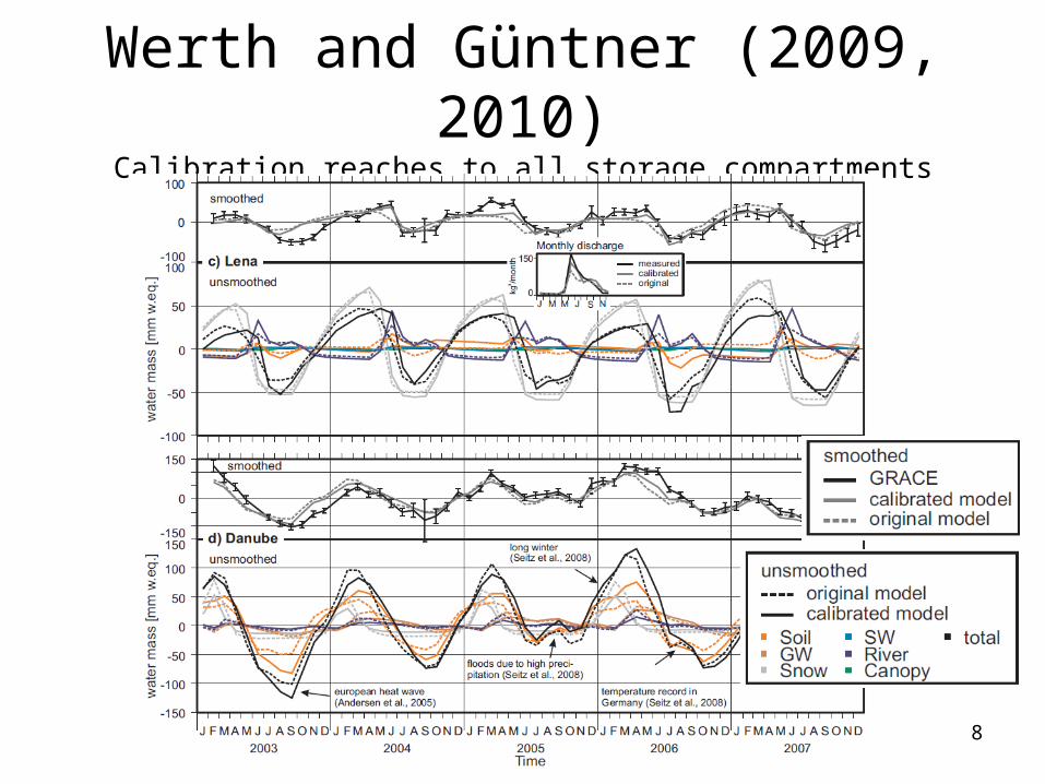
Werth and Güntner (2009, 2010)Calibration reaches to all storage compartments
8
Getirana (2010)
• MGB-IPH model for Amazon basin• Select 8 most relevant parameters based on sensitivity
analysis• Calibration data: ENVISAT altimetry (CTOH GDRs, ICE-1),
local gauge data• Different cost functions with 1-2 objectives (Nash-Sutcliffe
for anomalies, tangent and coefficient of regression)• MC optimization (MOCUM-UA for ensemble generation) • Pareto solution
• „…results demonstrate the potential of spatial altimetry for the automatic calibration of hydrological models in poorly gauged basins…“
9
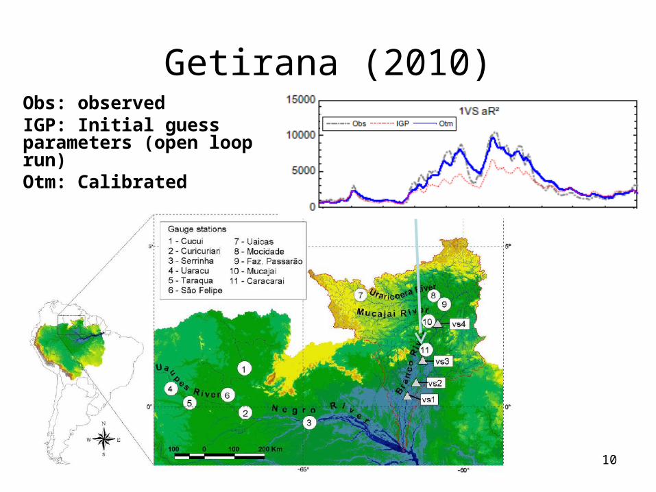
Getirana (2010)Obs: observedIGP: Initial guess parameters (open loop run)Otm: Calibrated
10
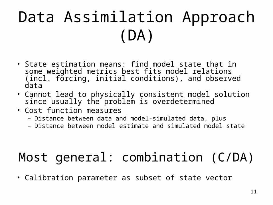
Data Assimilation Approach (DA)
• State estimation means: find model state that in some weighted metrics best fits model relations (incl. forcing, initial conditions), and observed data
• Cannot lead to physically consistent model solution since usually the problem is overdetermined
• Cost function measures– Distance between data and model-simulated data, plus– Distance between model estimate and simulated model state
Most general: combination (C/DA)
• Calibration parameter as subset of state vector 11
Zaitchik, Rodell, Reichle (2008), Li et al. (2012)
• Catchment LSM, works on topographically defined „catchments“ (avg. area 4000 km2), Mississippi, Europe, …
• Meteo forcing data: from GLDAS data base• Calibration data: GRACE basin average for sub-basins, (over-)
simplified error covariance• Validation data: Observed groundwater, river discharge• EnKF for near-realtime, EnKS (iterative application) for optimal
reanalysis, Ensemble: 20 members• Special scheme for temporally disaggregating monthly GRACE data• No explicit parameter calibration ?• State error covariance: includes propagated perturbations in
precipitation,radiation forcing and prognostic variables
• „…assimilation estimates of groundwater variability exhibit enhanced skill with respect to measured groundwater in all four subbasins“
12
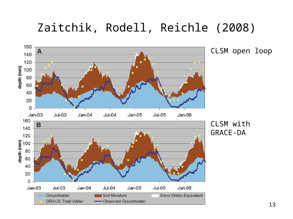
Zaitchik, Rodell, Reichle (2008)
CLSM open loop
CLSM with GRACE-DA
13
Working Hypothesis (II)
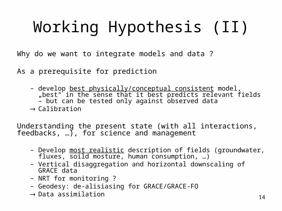
Why do we want to integrate models and data ?
As a prerequisite for prediction
– develop best physically/conceptual consistent model, „best“ in the sense that it best predicts relevant fields – but can be tested only against observed data
Calibration
Understanding the present state (with all interactions, feedbacks, …), for science and management
– Develop most realistic description of fields (groundwater, fluxes, soild mosture, human consumption, …)
– Vertical disaggregation and horizontal downscaling of GRACE data– NRT for monitoring ?– Geodesy: de-alisiasing for GRACE/GRACE-FO Data assimilation 14
Variational Assimilation (3D/4DVAR)
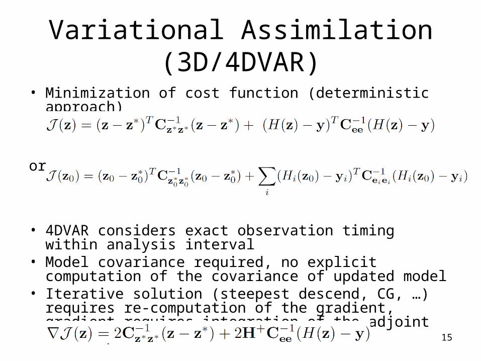
• Minimization of cost function (deterministic approach)
or
• 4DVAR considers exact observation timing within analysis interval
• Model covariance required, no explicit computation of the covariance of updated model
• Iterative solution (steepest descend, CG, …) requires re-computation of the gradient, gradient requires integration of the adjoint model operator H+
15
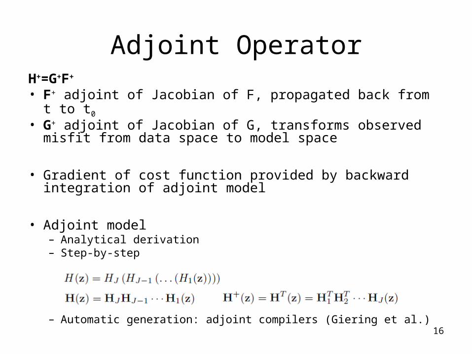
Adjoint OperatorH+=G+F+
• F+ adjoint of Jacobian of F, propagated back from t to t0• G+ adjoint of Jacobian of G, transforms observed misfit
from data space to model space
• Gradient of cost function provided by backward integration of adjoint model
• Adjoint model– Analytical derivation– Step-by-step
– Automatic generation: adjoint compilers (Giering et al.) 16
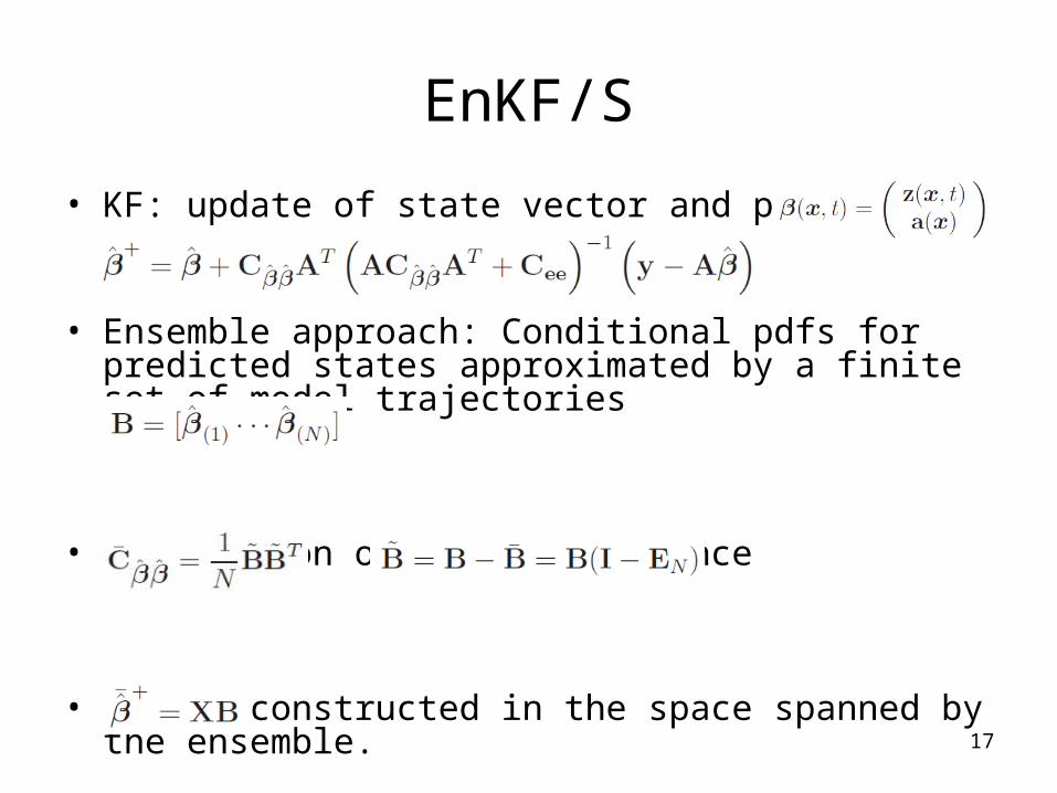
EnKF/S
• KF: update of state vector and parameter
• Ensemble approach: Conditional pdfs for predicted states approximated by a finite set of model trajectories
• Propagation of model covariance
• Update constructed in the space spanned by the ensemble.
17
EnKF/S
• Using future observation for optimal solution: EnKS
• The update is constructed in the space spanned by the ensemble. So, how big should be the ensemble?
• How should we initialize the ensemble in order to optimally „explore“ the model space?
• Though the EnKF involves full nonlinear model propagation and observation equations, it is based on 2nd-order statistics
• Technical issues– Data perturbation approach or square-root approach, for getting the
statistics right– Use assimilative framework (e.g. PDAF, Nerger)?
18
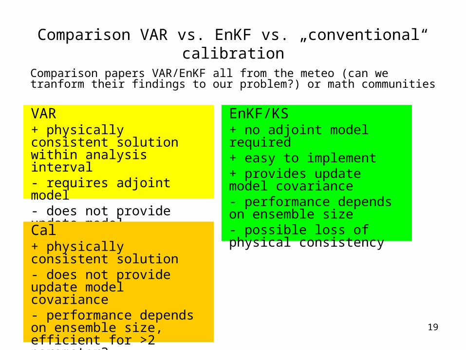
Comparison VAR vs. EnKF vs. „conventional“ calibration
Comparison papers VAR/EnKF all from the meteo (can we tranform their findings to our problem?) or math communities
VAR+ physically consistent solution within analysis interval- requires adjoint model- does not provide update model covariance
EnKF/KS+ no adjoint model required+ easy to implement+ provides update model covariance- performance depends on ensemble size- possible loss of physical consistencyCal
+ physically consistent solution- does not provide update model covariance- performance depends on ensemble size, efficient for >2 parameter?- no state adjustment 19
20
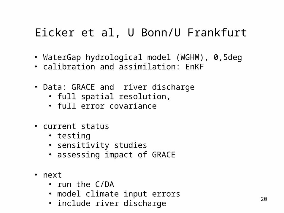
• WaterGap hydrological model (WGHM), 0,5deg• calibration and assimilation: EnKF
• Data: GRACE and river discharge• full spatial resolution, • full error covariance
• current status• testing• sensitivity studies• assessing impact of GRACE
• next• run the C/DA• model climate input errors• include river discharge
Eicker et al, U Bonn/U Frankfurt
20

k k kl A xobservations (GRACE)
llΣwith
Kalman filter
21
Kalman Filter
Total water storage(grid)
1 1k k k
x B xprediction (model):
xxΣwith
Full covariance matrix(grid)
GRACE monthly solutions
• ITG-Grace2010• spherical harm. Nmax=60• full covariance matrix
0.5°x0.5° grid
27 calibration parameters+
CANOPYSNOWSOILLAKE (local)WETLAND (local)LAKE (global)WETLAND (global)RESERVOIRRIVERGROUNDWATER
10 compartments:
21
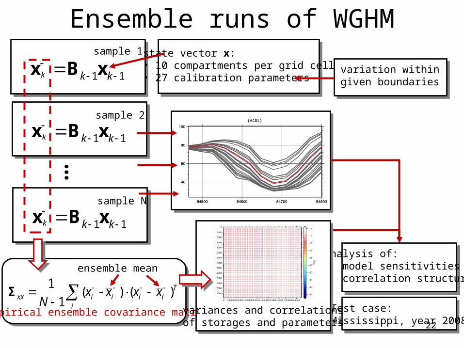
Ensemble runs of WGHM
22
1 1k k k
x B xsample 1
1 1k k k
x B x
1 1k k k
x B x
…
sample 2
sample N
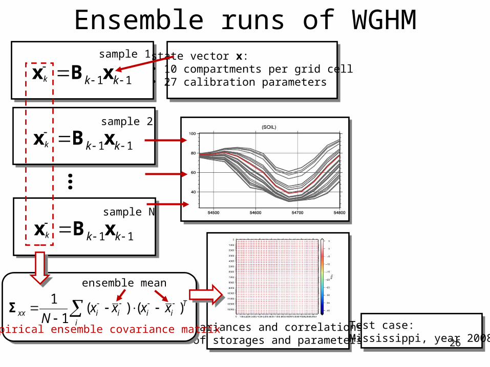
state vector x:• 10 compartments per grid cell• 27 calibration parameters
analysis of:• model sensitivities• correlation structures
Test case:Mississippi, year 2008
empirical ensemble covariance matrix
ensemble mean
Tiii
iixx xxxx
N)()(
1
1
Σvariances and correlations of storages and parameters
variation within given boundaries
22
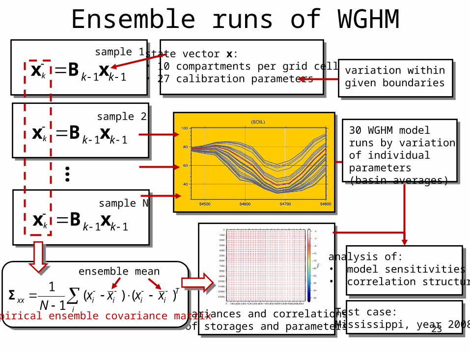
Ensemble runs of WGHM
23
1 1k k k
x B xsample 1
1 1k k k
x B x
1 1k k k
x B x
…
sample 2
sample N
state vector x:• 10 compartments per grid cell• 27 calibration parameters
variances and correlations of storages and parameters
analysis of:• model sensitivities• correlation structures
Test case:Mississippi, year 2008
30 WGHM model runs by variation of individual parameters(basin averages)
empirical ensemble covariance matrix
ensemble mean
Tiii
iixx xxxx
N)()(
1
1
Σ
variation within given boundaries
23
24river
wetland
total water storage
wat
er
hei
ght
[mm
]
date [MJD]
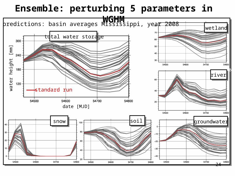
Ensemble: perturbing 5 parameters in WGHM
groundwatersnow soil
standard run
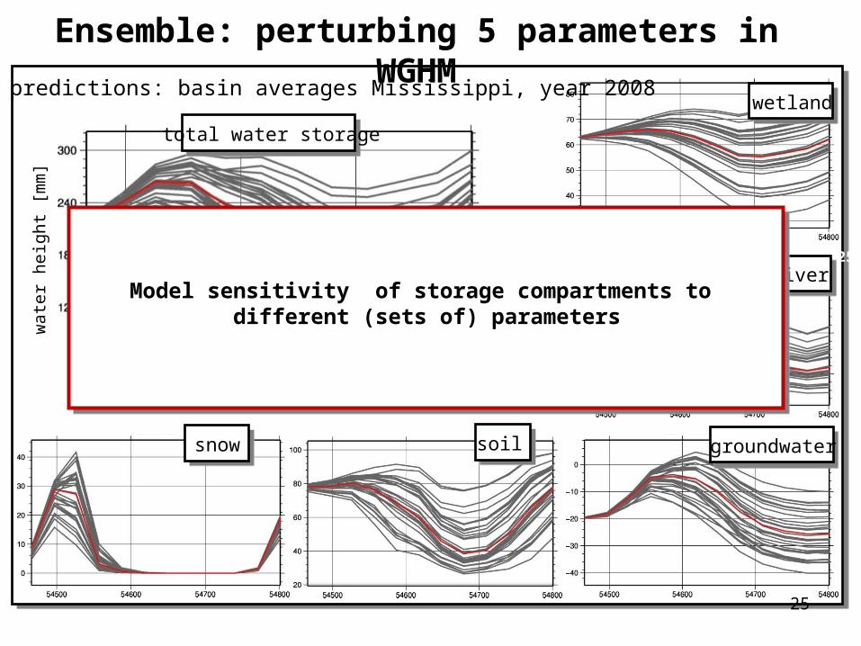
Model predictions: basin averages Mississippi, year 2008
24
25river
wetland
total water storage
wat
er
hei
ght
[mm
]
date [MJD]
groundwatersnow soil
standard run
Model predictions: basin averages Mississippi, year 2008
Model sensitivity of storage compartments to different (sets of) parameters
Ensemble: perturbing 5 parameters in WGHM
25
Ensemble runs of WGHM
26
1 1k k k
x B xsample 1
1 1k k k
x B x
1 1k k k
x B x
…
sample 2
sample N
state vector x:• 10 compartments per grid cell• 27 calibration parameters
variances and correlations of storages and parameters
Test case:Mississippi, year 2008
empirical ensemble covariance matrix
ensemble mean
Tiii
iixx xxxx
N)()(
1
1
Σ
26
Ensemble runs of WGHM
27
1 1k k k
x B xsample 1
1 1k k k
x B x
1 1k k k
x B x
…
sample 2
sample N
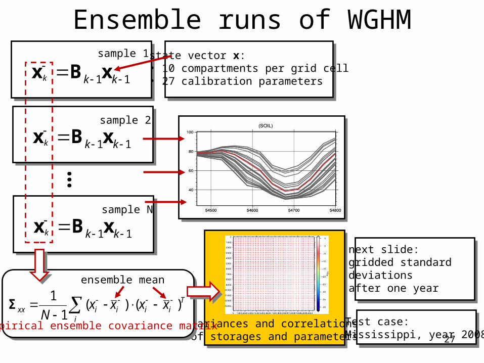
state vector x:• 10 compartments per grid cell• 27 calibration parameters
variances and correlations of storages and parameters
next slide:gridded standard deviationsafter one year
Test case:Mississippi, year 2008
empirical ensemble covariance matrix
ensemble mean
Tiii
iixx xxxx
N)()(
1
1
Σ
27
28
groundwatersnow soil
riverwetland
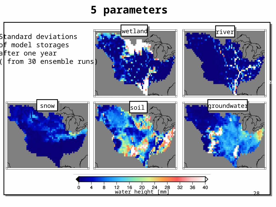
5 parameters
water height [mm]
Standard deviations of model storages after one year( from 30 ensemble runs)
28

29
groundwatersnow soil
riverwetland
5 parameters
water height [mm]
Standard deviations of model storages after one year( from 30 ensemble runs)
Varying spatial distribution of model uncertainties in different compartments
29
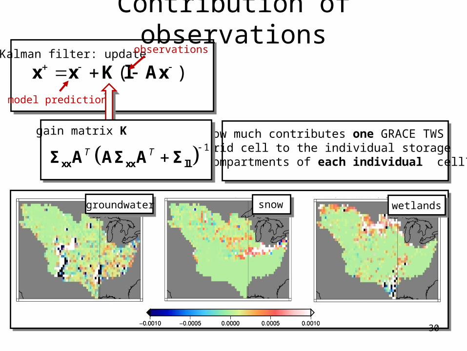
Contribution of observations
30
( ) x x K l AxKalman filter: update observations
model prediction
How much contributes one GRACE TWS grid cell to the individual storage compartments of each individual cell?
groundwater snow wetlands
1T T xx xx llΣ A AΣ A Σ
gain matrix K
30
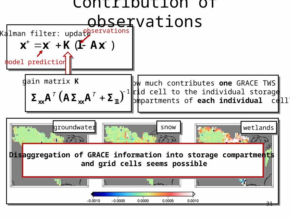
Contribution of observations
31
( ) x x K l AxKalman filter: update observations
model prediction
How much contributes one GRACE TWS grid cell to the individual storage compartments of each individual cell?
groundwater snow wetlands
1T T xx xx llΣ A AΣ A Σ
gain matrix K
Disaggregation of GRACE information into storage compartments and grid cells seems possible
31

Contribution of observations
32
( ) x x K l AxKalman filter: update observations
model prediction
1T T xx xx llΣ A AΣ A Σ
gain matrix K How much contribute all GRACE TWS grid cell to the basin average of each storage compartment?
Apply averaging operator:
( ) Mx Mx MK l Ax
basin averagefor each compartment
contribution of each GRACE cell observation to basin average
sum of weights
32
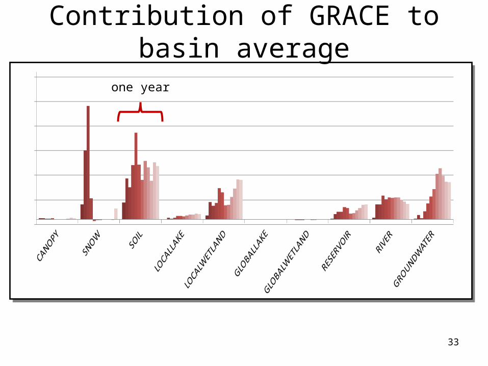
Contribution of GRACE to basin average
33
one year
33
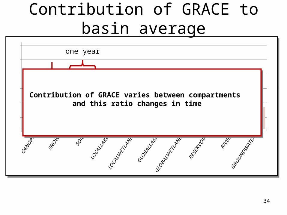
Contribution of GRACE to basin average
34
one year
Contribution of GRACE varies between compartments and this ratio changes in time
34
Key questions
Key questions that need to be answered– How should we use the new types of data (GRACE, altimetric
level, …) cf. new IAG WG Land hydrology from gravimetry– What components of modeling can be improved through C/DA– How will we characterize model noise and forcing data noise– How will we deal with systematic model and forcing data errors– How can we test data-integrated modeling– How far can we improve understanding of the present state of
the freshwater system– How far can we improve simulations
– Can we formulate recommendations for upcoming and future systems (e.g. see current discussion on Sentinel-3 SAR/LRM coverage inland/oceans)
35