integrated navigation, guidance, and control of missile ... · pdf fileunclassified...
TRANSCRIPT

UNCLASSIFIED
Integrated Navigation, Guidance, and Control of Missile Systems: 2-D Dynamic Models
Farhan A. Faruqi
Weapons Systems Division Defence Science and Technology Organisation
DSTO-TR-2706
ABSTRACT In this report mathematical models (2-D Azimuth and Elevation Planes) for multi-party engagement kinematics are derived suitable for developing, implementing and testing modern missile guidance systems. The models developed here are suitable for both conventional and more advanced optimal intelligent guidance schemes including those that arise out of the differential game theory. These models accommodate changes in vehicle body attitude and other non-linear effects such as limits on lateral acceleration and aerodynamic forces.
RELEASE LIMITATION
Approved for public release
UNCLASSIFIED
UNCLASSIFIED
Published by Weapons Systems Division DSTO Defence Science and Technology Organisation PO Box 1500 Edinburgh South Australia 5111 Australia Telephone: (08) 7389 5555 Fax: (08) 7389 6567 © Commonwealth of Australia 2012 AR-015-302 May 2012 APPROVED FOR PUBLIC RELEASE
UNCLASSIFIED
UNCLASSIFIED
UNCLASSIFIED
Integrated Navigation, Guidance, and Control of Missile Systems: 2-D Dynamic Models
Executive Summary In the past, linear kinematics models have been used for development and analysis of guidance laws for missile/target engagements. These models were developed in fixed axis systems under the assumption that the engagement trajectory does not vary significantly from the collision course geometry. While these models take into account autopilot lags and acceleration limits, the guidance commands are applied in fixed axis, and ignore the fact that the missile/target attitude may change significantly during engagement. This latter fact is particularly relevant in cases of engagements where the target implements evasive manoeuvres, resulting in large variations of the engagement trajectory from that of the collision course. The linearised models are convenient for deriving guidance laws (in analytical form), however, the study of their performance characteristics still requires a non-linear model that incorporates changes in body attitudes and implements guidance commands in body axis rather than the fixed axis. In this report, azimuth and elevation plane mathematical models for multi-party engagement kinematics are derived suitable for developing, implementing and testing modern missile guidance systems. The models developed here are suitable for both conventional and more advanced optimal intelligent guidance, particularly those based on the 'game theory' guidance techniques. These models accommodate changes in vehicle body attitude and other non-linear effects, such as, limits on lateral acceleration and aerodynamic forces. The models presented in this report will be found suitable for computer simulation and analysis of multi-party engagements.

UNCLASSIFIED
UNCLASSIFIED
This page is intentionally blank
UNCLASSIFIED
UNCLASSIFIED
Author
Dr. Farhan A. Faruqi Weapons Systems division Farhan A. Faruqi received B.Sc.(Hons) in Mechanical Engineering from the University of Surrey (UK), 1968; M.Sc. in Automatic Control from the University of Manchester Institute of Science and Technology (UK), 1970 and Ph.D from the Imperial College, London University (UK), 1973. He has over 25 years experience in the Aerospace and Defence Industry in UK, Europe and the USA. Prior to joining DSTO in January 1999 he was an Associate Professor at QUT (Australia) 1993-98. Dr. Faruqi is currently with the Guidance and Control Group, Weapons Systems Division, DSTO. His research interests include: Missile Navigation, Guidance and Control, Target Tracking and Precision Pointing Systems, Strategic Defence Systems, Signal Processing, and Optoelectronics.
____________________ ________________________________________________

UNCLASSIFIED
UNCLASSIFIED
This page is intentionally blank
UNCLASSIFIED DSTO-TR-2706
Contents
NOMENCLATURE
1. INTRODUCTION............................................................................................................... 1
2. DEVELOPMENT OF AZIMUTH PLANE ENGAGEMENT KINEMATICS MODEL ................................................................................................................................. 1 2.1 Translational Kinematics for Multi-Vehicle Engagement................................ 1
2.1.1 Vector/Matrix Representation .............................................................. 2 2.2 Constructing Relative Sightline (LOS) Angles and Rates - (Rotational
Kinematics) ................................................................................................................ 3 2.3 Vehicle Navigation Model ...................................................................................... 4 2.4 Vehicle Autopilot Dynamics .................................................................................. 5
3. GUIDANCE LAWS............................................................................................................. 6 3.1 Proportional Navigation (PN) Guidance.............................................................. 6 3.2 Augmented Proportional Navigation (APN) Guidance .................................... 7
4. OVERALL AZIMUTH PLANE STATE SPACE MODEL............................................ 7
5. EXTENSION TO ELEVATION PLANE ENGAGEMENT MODEL.......................... 8 5.1 Translational Kinematics for Multi-Vehicle Engagement................................ 8 5.2 Constructing Relative Sightline (LOS) Angles and Rates - (Rotational
Kinematics) ................................................................................................................ 9 5.3 Vehicle Navigation Model .................................................................................... 10 5.4 Vehicle Autopilot Dynamics ................................................................................ 11 5.5 Guidance Laws-PN and APN Guidance............................................................. 12 5.6 Overall State Space Model in Elevation Plane.................................................. 13
6. CONCLUSIONS................................................................................................................ 14
7. REFERENCES .................................................................................................................... 14
8. ACKNOWLEDGEMENTS .............................................................................................. 14
UNCLASSIFIED
UNCLASSIFIED DSTO-TR-2706
List of Tables
Table 1: Combined (Yaw-Plane) State Space Dynamics Model for Navigation, Seeker, Guidance and Autopilot................................................................................................................ 15 Table 2: Combined (Pitch-Plane) State Space Dynamics Model for Navigation, Seeker, Guidance and Autopilot................................................................................................................ 16
List of Figures
Figure 1: Engagement Geometry for 2-Vehicles ........................................................................ 17 Figure 2: Axis transformation fixed <=>body in pitch-plane .................................................. 17 Figure 3: Body Incidence .............................................................................................................. 18 Figure 4: Axis System Convention............................................................................................... 18 Figure 5: Axis transformation fixed <=>body in pitch-plane .................................................. 19 Figure 6: Yaw-Plane Simulation Model Block Diagram ........................................................... 20 Figure 7: Pitch-Plane Simulation Model Block Diagram .......................................................... 21 Figure A.1. Aerodynamic variables for a missile....................................................................... 25
UNCLASSIFIED

UNCLASSIFIED DSTO-TR-2706
Nomenclature :j,i number of interceptors (pursuers) and targets (evaders) respectively. :z,y,x iii are x , y, z-positions respectively of vehicle i in fixed axis. :w,v,u iii are x, y, z-velocities respectively of vehicle i in fixed axis. :a,a,a
iziyix are x, y, z-accelerations respectively of vehicle i in fixed axis.
:z,y,x jijiji are x, y, z-positions respectively of vehicle j w.r.t i in fixed axis.
:w,v,u jijiji are x, y, z-velocities respectively of vehicle j w.r.t i in fixed axis.
:a,a,ajizjiyjix are x, y, z-accelerations respectively of vehicle j w.r.t i in fixed
axis. :a,u,x iii are x ,y-position, velocity and acceleration vectors of vehicle i in
fixed axis. :a,u,x jijiji are x, y- relative position, velocity and acceleration vectors of vehicle
j w.r.t i in fixed axis. :c,v,y iii
are x, z-position, velocity and acceleration vectors of vehicle i in
fixed axis.
:c,v,y jijiji
are x, z- relative position, velocity and acceleration vectors of vehicle
j w.r.t i in fixed axis. :R ji separation range of vehicle j w.r.t i in fixed axis.
:Vjic closing velocity of vehicle j w.r.t i in fixed axis.
:, jiji are line-of-sight angle (LOS) of vehicle j w.r.t i in yaw and pitch
planes respectively.
:a,a,a biz
biy
bix
x, y, z-accelerations respectively achieved by vehicle i in body axis.
:a,a,a b
dizb
diyb
dix
x, y, z-accelerations respectively demanded by vehicle i in body
axis.
:c,a bi
bi is the achieved missile acceleration vector in body axis.
:c,a bdi
bdi
is the demanded missile acceleration vector in body axis.
:, ii are yaw and pitch body (Euler) angles respectively of the ith vehicle w.r.t the fixed axis.
:T ifb is the transformation matrix from body axis to fixed axis.
:Vi is the velocity of vehicle i. :
ix autopilot's longitudinal time-constant for vehicle i.
:,iziy autopilot's lateral time-constant for vehicle i.
UNCLASSIFIED

UNCLASSIFIED DSTO-TR-2706
UNCLASSIFIED
This page is intentionally blank
UNCLASSIFIED DSTO-TR-2706
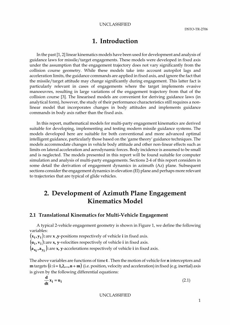
1. Introduction
In the past [1, 2] linear kinematics models have been used for development and analysis of guidance laws for missile/target engagements. These models were developed in fixed axis under the assumption that the engagement trajectory does not vary significantly from the collision course geometry. While these models take into account autopilot lags and acceleration limits, the guidance commands are applied in fixed axis, and ignore the fact that the missile/target attitude may change significantly during engagement. This latter fact is particularly relevant in cases of engagements where the target implements evasive manoeuvres, resulting in large variations of the engagement trajectory from that of the collision course [3]. The linearised models are convenient for deriving guidance laws (in analytical form), however, the study of their performance characteristics still requires a non-linear model that incorporates changes in body attitudes and implements guidance commands in body axis rather than the fixed axis. In this report, mathematical models for multi-party engagement kinematics are derived suitable for developing, implementing and testing modern missile guidance systems. The models developed here are suitable for both conventional and more advanced optimal intelligent guidance, particularly those based on the 'game theory' guidance techniques. The models accommodate changes in vehicle body attitude and other non-linear effects such as limits on lateral acceleration and aerodynamic forces. Body incidence is assumed to be small and is neglected. The models presented in this report will be found suitable for computer simulation and analysis of multi-party engagements. Sections 2-4 of this report considers in some detail the derivation of engagement dynamics in azimuth (Az) plane. Subsequent sections consider the engagement dynamics in elevation (El) plane and perhaps more relevant to trajectories that are typical of glide vehicles.
2. Development of Azimuth Plane Engagement Kinematics Model
2.1 Translational Kinematics for Multi-Vehicle Engagement
A typical 2-vehicle engagement geometry is shown in Figure 1, we define the following variables: :y,x ii are x ,y-positions respectively of vehicle i in fixed axis. :v,u ii are x, y-velocities respectively of vehicle i in fixed axis. :a,a
iyix are x, y-accelerations respectively of vehicle i in fixed axis.
The above variables are functions of time . Then the motion of vehicle for n interceptors and m targets
t mn,...,2,1i:i (i.e. position, velocity and acceleration) in fixed (e.g. inertial) axis
is given by the following differential equations:
ii uxdt
d (2.1)
UNCLASSIFIED 1
UNCLASSIFIED DSTO-TR-2706
ii vydt
d (2.2)
ixi audt
d (2.3)
iyi avdt
d (2.4)
For multiple vehicles i, j engagement, we define the relative variables (states) for ij;m,...,2,1j;n,...,2,1i:i as follows:
:xxx ijji x-position of vehicle j w.r.t i in fixed axis.
:yyy ijji y-position of vehicle j w.r.t i in fixed axis.
:uuu ijji x-velocity of vehicle j w.r.t i in fixed axis.
:vvv ijji y-velocity of vehicle j w.r.t i in fixed axis.
:aaaixjxjix x-acceleration of vehicle j w.r.t i in fixed axis.
:aaa yijyjiy y-acceleration of vehicle j w.r.t i in fixed axis.
2.1.1 Vector/Matrix Representation
We can write equations (2.1)-(2.4), in vector notation as:
ii uxdt
d (2.5)
ii audt
d (2.6)
Where:
:yxx Tiii is the position vector of vehicle i in fixed axis.
:vuu Tiii is the velocity vector of vehicle i in fixed axis.
:aaa Tiyixi is the target acceleration vector of vehicle i in fixed axis.
Similarly, we can write the relative kinematics vector equations as:
jiji uxdt
d (2.7)
ijji aaudt
d (2.8)
Where:
:yxx Tjijiji position vector of vehicle j w.r.t i in fixed axis.
:vuu Tjijiji velocity vector of vehicle j w.r.t i in fixed axis.
:aaaaa ijT
jiyjixji acceleration vector of vehicle j w.r.t i in fixed axis.
UNCLASSIFIED 2
UNCLASSIFIED DSTO-TR-2706
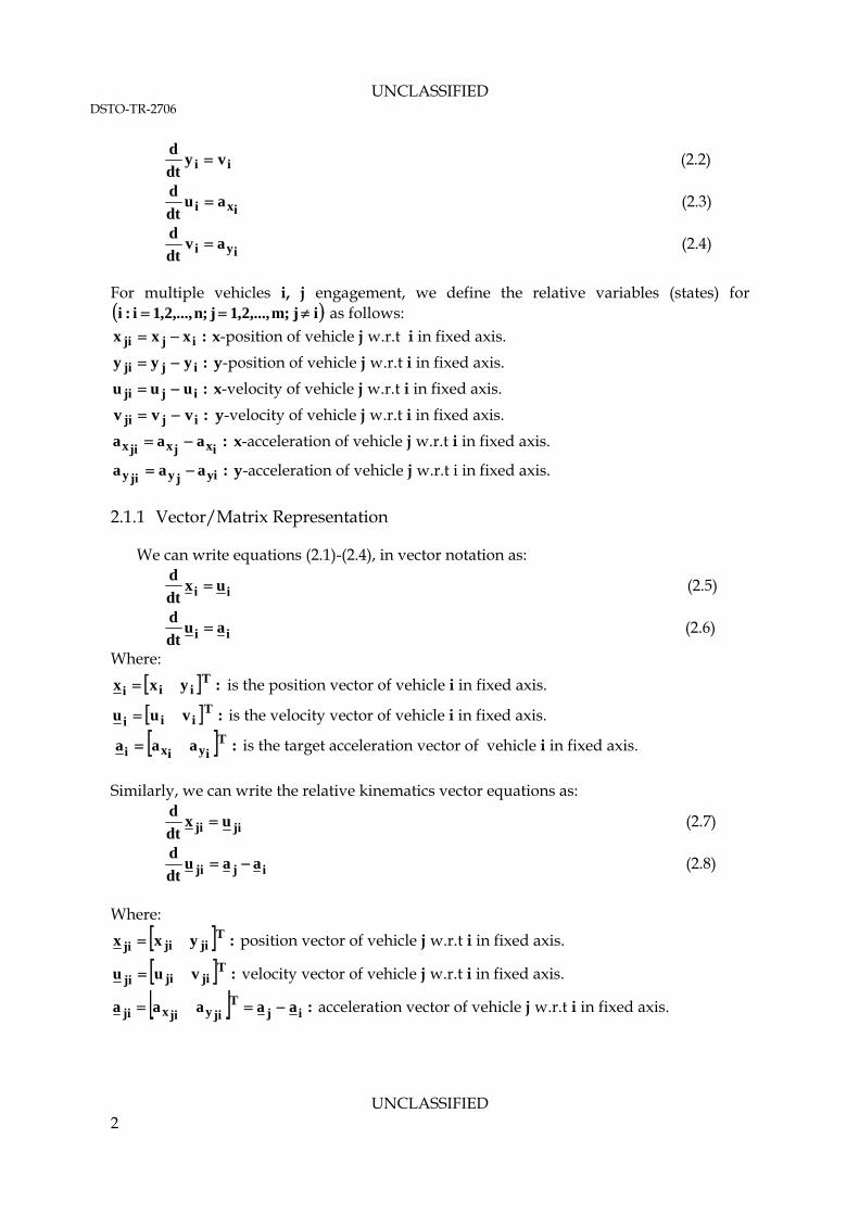
Note: The above formulation admits consideration of engagement where one particular vehicle (interceptor) is fired at another single vehicle (target). In other words we consider one-against-one in a scenario consisting of many vehicles. This consideration can be extended to one-against-many if, for example, i takes on a single value and j is allowed to take on a number of different values. 2.2 Constructing Relative Sightline (LOS) Angles and Rates - (Rotational Kinematics)
The separation range between vehicles j w.r.t i is given by: jiR
2
1
jiT
ji2
12
ji2
jiji xxyxR (2.9)
The range rate is given by: jiR
ji
jiT
ji
ji
jijijijijiji R
ux
R
vyuxRR
dt
d
(2.10)
The Closing Velocity is given by:
jicV
jijic RV (2.11)
The sightline angle of j w.r.t i is given by: ji
ji
jiji x
ytan (2.12)
Differentiating both sides of the equation and simplifying, we get:
2
ji
jiT
ji
2ji
jijijiji
2ji
jiji
2ji
jijijiji
R
uJx
R
uyvx
R
xy
R
xy
dt
d
(2.13)
Where:
01
10J
Note that an approximation to (2.13) is sometimes used, although not recommended for simulation purposes, based on the assumptions that the engagement geometry does not deviate significantly from the collision course; in this case:
gojicjiji TVRx ; ; jicjiji VRx :ttT fgo is the time-to-go.
Substituting this in equation (2.13) gives us:
2go
ji
go
ji
jicji
T
y
T
y
V
1 (2.14)
UNCLASSIFIED 3
UNCLASSIFIED DSTO-TR-2706
The measurements obtained from the seeker that are used to construct the guidance
commands are given by: ji
jijijiˆ
(2.15)
Where:
:ji seeker LOS rate measurement error.
The above relationships (2.9)-(2.15) will also be referred to as the seeker model. 2.3 Vehicle Navigation Model
Let us define the following:
:abix x-acceleration achieved by vehicle i in its body axis.
:abiy y-acceleration achieved by vehicle i in its body axis.
The transformation from fixed to body axis is given by (see Figure 2):
iy
ixi
bf
iy
ix
ii
iib
iy
bix
a
aT
a
a
cossin
sincos
a
a (2.16)
In vector/matrix notation this equation may be written as:
iibf
bi aTa (2.17)
bii
fbi aTa (2.18)
Where:
i : is the yaw (Euler) angle of the ith vehicle w.r.t the fixed axis. It is assumed that the body orientation changes during the engagement. i
:aaaT
biy
bix
bi
is acceleration vector of vehicle i in its body axis.
is the transformation matrix from body axis to fixed axis. :TTT1
ibf
T
ibfi
fb
:cossin
sincosT
ii
iii
fb
is the (direction cosine) transformation matrix from body to fixed
axis. The vehicle velocity is given by:
2
1
iT
i2
12
i2
ii uuvuV (2.19)
UNCLASSIFIED 4
UNCLASSIFIED DSTO-TR-2706
Now the flight path angle (=angle that the velocity vector makes with the fixed axis) is given by:
i
iii u
vtan (2.20)
Where:
:u
vtan
b
b1i
is the azimuth body incidence (side-slip angle), bb v,u are body axis
velocities (Figure A1.1).
Differentiating both sides of equation (2.20) and simplifying we get:
2
i
iT
i2
i
ixiiyi
2i
ii2
i
iiii
V
aJu
V
avau
V
uv
V
uv
(2.21)
Assuming remain small ( ; see also Appendix A), then we may write: ii ,
bb vu
2
i
iT
i2
i
ixiiyi
2i
ii2
i
iii
V
aJu
V
avau
V
uv
V
uv
dt
d
(2.22)
2.4 Vehicle Autopilot Dynamics
Assuming a first order lag for the autopilot, we may write for vehicle i: b
dixixbixix
bix aaa
dt
d (2.23)
b
diyiyb
iyiyb
iy aaadt
d (2.24)
In vector/matrix notation equations (2.23), (2.24) may be written as:
bdii
bii
bi aaa
dt
d (2.25)
Where:
:ix Vehicle i autopilot's longitudinal time-constant.
:iy Vehicle i autopilot's lateral time-constant.
iy
ixi 0
0
:ab
dix x-acceleration demanded by vehicle i in its body axis.
:ab
diy y-acceleration demanded by vehicle i in its body axis.
:aaaT
b
diyb
dixbdi
is the demanded missile acceleration (command input) vector in body
axis.
UNCLASSIFIED 5
UNCLASSIFIED DSTO-TR-2706
Remarks: Detailed consideration of the effects of the aerodynamic forces is contained in
Appendix A. Generally, the longitudinal acceleration i
iib
dix m
DTa
of a missile is not
varied in response to the guidance commands and may be assumed to be zero. However, the
nominal values:
m
DTab
ix
will change due to changes in flight conditions and needs to be
included in the simulation model; this is shown in the block diagram Figure 6. The limits on
the lateral acceleration can be implemented as: maxydiy
b aa (see Appendix A).
3. Guidance Laws
3.1 Proportional Navigation (PN) Guidance
There are at least three versions of PN guidance laws that the author is aware of; these are (for vehicle i - the pursuer against an intercept (target) vehicle j – the evader): 3.1.1. Version 1 (PN-1): This implementation is based on the principle that the demanded body rate of the attacker i is proportional to LOS rate to the target j (see Figure 1); that is:
jidi N (3.1)
Where: is the navigation constant. Thus the demanded attacker lateral acceleration is given by:
:N
jiidiib
diy NVVa (3.2)
i
iib
dix m
DTa
(3.3)
3.1.2. Version 2 (PN-2): This implementation is based on the principle that the demanded lateral acceleration of the attacker i is proportional to the acceleration perpendicular (normal) to the LOS rate to the target j. Now the acceleration normal to the LOS is given by:
jijicjin Va (3.4)
jijicjinb
diy NVNaa (3.5)
i
iib
dix m
DTa
(3.6)
Where:
UNCLASSIFIED 6
UNCLASSIFIED DSTO-TR-2706
:RV jijic is the 'closing velocity' between the attacker and the target.
:ajin is the acceleration normal to the LOS.
3.1.3. Version 3 (PN-3): This type of guidance law is similar to version 2 except that the normal LOS acceleration is resolved along the lateral direction to the attacker body axis first before applying the proportionality principal. Thus, we have:
jijicjin Va (3.7)
giving us the guidance commands:
jijiijicjiijinb
diy cosNVcosNaa (3.8)
i
iib
dix m
DTa
(3.9)
3.2 Augmented Proportional Navigation (APN) Guidance
Finally, a variation of the PN guidance law is the APN that can be implemented as follows:
jibf
bdi
aTNPNGa (3.10)
Where:
:N is the (target) acceleration navigation constant :PNG is the proportional navigation guidance law given in (3.1)-(3.7) Remarks
Seeker errors can be introduced by replacing by in the guidance laws above. ji ji
In certain engagement geometries sin(..),..cos,Vjic and terms in the above equations
may become zero prior to termination of the engagements, particularly for manoeuvring targets, and it may become necessary to apply additional disturbances to achieve successful intercept.
ji
4. Overall Azimuth Plane State Space Model
The overall non-linear state space model (e.g. for APN guidance) that can be used for sensitivity studies and for non-linear or Monte-Carlo analysis is given below:
jiji uxdt
d (4.1)
bii
fb
bjj
fbji aTaTu
dt
d (4.2)
UNCLASSIFIED 7
UNCLASSIFIED DSTO-TR-2706
jiT
ji
jiT
jiji
xx
uJx
dt
d (4.3)
jibf
bdi
aTNPNGa (4.4)
bdii
bii
bi aaa
dt
d (4.5)
i
Ti
iT
iii
uu
aJu
dt
d (4.6)
The overall state space model that can be implemented on the computer is given in Table 4.1, and the block-diagram is shown in Figure 6.
5. Extension to Elevation Plane Engagement Model
The axis transformation diagram is shown in Figure 4. We shall point out the fact that the order of rotation is in the order (yaw, pitch and roll), i.e. . Of course for a 2-D yaw–pitch decoupled model , however, we shall continue to follow this convention for the derivation given in this report. Figures 2 and 5 depict the yaw and pitch transformation diagrams separately. It will be noted, therefore, the key differences in the yaw and the pitch derivation is the transformation matrix, and the steady-state aerodynamic forces acting in the two planes.
0
5.1 Translational Kinematics for Multi-Vehicle Engagement
The development of the elevation (El) plane model follows closely the methodology used in the development of the Az model; we define the following variables: :z,x ii are x ,z-positions respectively of vehicle i in fixed axis. :w,u ii are x, z-velocities respectively of vehicle i in fixed axis. :a,a
izix are x, z-accelerations respectively of vehicle i in fixed axis.
The motion of vehicle for n interceptors and m targets mn,...,2,1i:i (i.e. position, velocity and acceleration) in fixed (e.g. inertial) axis is given by the following differential equations:
ii uxdt
d (5.1)
ii wzdt
d (5.2)
ixi audt
d (5.3)
izi awdt
d (5.4)
UNCLASSIFIED 8
UNCLASSIFIED DSTO-TR-2706
For multiple vehicles i, j engagement, we define the relative variables (states) for m,...,2,1j;n,...,2,1i:i as follows:
:xxx ijji x-position of vehicle j w.r.t i in fixed axis.
:zzz ijji z-position of vehicle j w.r.t i in fixed axis.
:uuu ijji x-velocity of vehicle j w.r.t i in fixed axis.
:www ijji z-velocity of vehicle j w.r.t i in fixed axis.
:aaajxjxjix x-acceleration of vehicle j w.r.t i in fixed axis.
:aaa zijzjiz z-acceleration of vehicle j w.r.t i in fixed axis.
5.1.1. Vector/Matrix Representation We can write equations (5.1)-(5.4), in vector notation as:
iivy
dt
d (5.5)
ii cvdt
d (5.6)
Similarly, we can write the relative kinematics vector equations as:
jijivy
dt
d (5.7)
ijji ccvdt
d (5.8)
Where:
:zxy Tiii
is the position vector of vehicle i in fixed axis.
:wuv Tiii is the velocity vector of vehicle i in fixed axis.
:aac Tizixi is the target acceleration vector of vehicle i in fixed axis.
:zxy Tjijiji
position vector of vehicle j w.r.t i in fixed axis.
:wuv Tjijiji velocity vector of vehicle j w.r.t i in fixed axis.
:ccaac ijT
jizjixji acceleration vector of vehicle j w.r.t i in fixed axis.
5.2 Constructing Relative Sightline (LOS) Angles and Rates - (Rotational Kinematics)
The separation range between vehicles j w.r.t i is given by: jiR
2
1
jiT
ji2
12
ji2
jiji yyzxR
(5.9)
The range rate is given by: jiR
UNCLASSIFIED 9
UNCLASSIFIED DSTO-TR-2706
ji
jiT
ji
ji
jijijijijiji R
vy
R
wzuxRR
dt
d
(5.10)
The Closing Velocity is given by: cjiV
jijic RV (5.11)
The sightline angle of j w.r.t i is given by: ji
ji
jiji x
ztan (5.12)
Differentiating both sides and simplifying, gives us:
2
ji
jiT
ji
2ji
jijijiji
2ji
jiji
2ji
jijijiji
R
vJy
R
uzwx
R
xz
R
xz
dt
d
(5.13)
Note that an approximation to (5.13) is sometimes used, although not recommended for simulation purposes, based on the assumptions that the engagement geometry does not deviate significantly from the collision course; in this case:
gojicjiji TVRx ; ; jicjiji VRx :ttT fgo is the time-to-go.
Substituting this in equation (5.13) gives us:
2go
ji
go
ji
jicji
T
z
T
z
V
1 (5.14)
The measurements obtained from the seeker that are used to construct the guidance
commands are given by: ji
jijijiˆ (5.15)
Where:
:ji seeker LOS rate measurement error.
The above relationships (5.9)-(5.15) will also be referred to as the seeker model. 5.3 Vehicle Navigation Model
Let us define the following:
:abix x-acceleration achieved by vehicle i in its body axis.
:abiz y-acceleration achieved by vehicle i in its body axis.
The transformation from fixed to body axis is given by (see Figure 2):
UNCLASSIFIED 10
UNCLASSIFIED DSTO-TR-2706
iz
ixi
bf
iy
ix
ii
iibiz
bix
a
aT
a
a
cossin
sincos
a
a (5.16)
In vector/matrix notation this equation may be written as:
iibf
bi cTc (5.17)
bii
fbi cTc (5.18)
Where:
i : body (Euler) angle of the ith vehicle w.r.t the fixed axis.
:aacT
biy
bix
bi
is acceleration vector of vehicle i in its body axis.
is the transformation matrix from body axis to fixed axis. :TTT1
ibf
T
ibfi
fb
:cossin
sincosT
ii
iii
fb
is the (direction cosine) transformation matrix.
The vehicle velocity is given by:
2
1
iT
i2
12
i2
ii vvwuV (5.19)
The body flight path angle is given by:
i
iii u
wtan
Where: is the body angle of incidence angle. :i Differentiating both sides and simplifying and assuming (as in section 2.3) that are small, we get:
ii ,
2
i
iT
i2
i
ixiizi
2i
ii2
i
iiii
V
cJv
V
awau
V
uw
V
uw
dt
d
(5.20)
5.4 Vehicle Autopilot Dynamics
Assuming a first order lag for the autopilot, we may write for vehicle i: b
dixixbixix
bix aaa
dt
d (5.21)
b
dizizbiziz
biz aaa
dt
d (5.22)
In vector/matrix notation equations (5.21), (5.22) may be written as:
UNCLASSIFIED 11
UNCLASSIFIED DSTO-TR-2706
bdii
bii
bi ccc
dt
d (5.23)
Where:
:ix Vehicle i autopilot's longitudinal time-constant.
:iz Vehicle i autopilot's lateral time-constant.
iz
ixi 0
0
:ab
dix x-acceleration demanded by vehicle i in its body axis.
:ab
diz y-acceleration demanded by vehicle i in its body axis.
:aacT
b
dizb
dixbdi
is the demanded missile acceleration (command input) vector in body
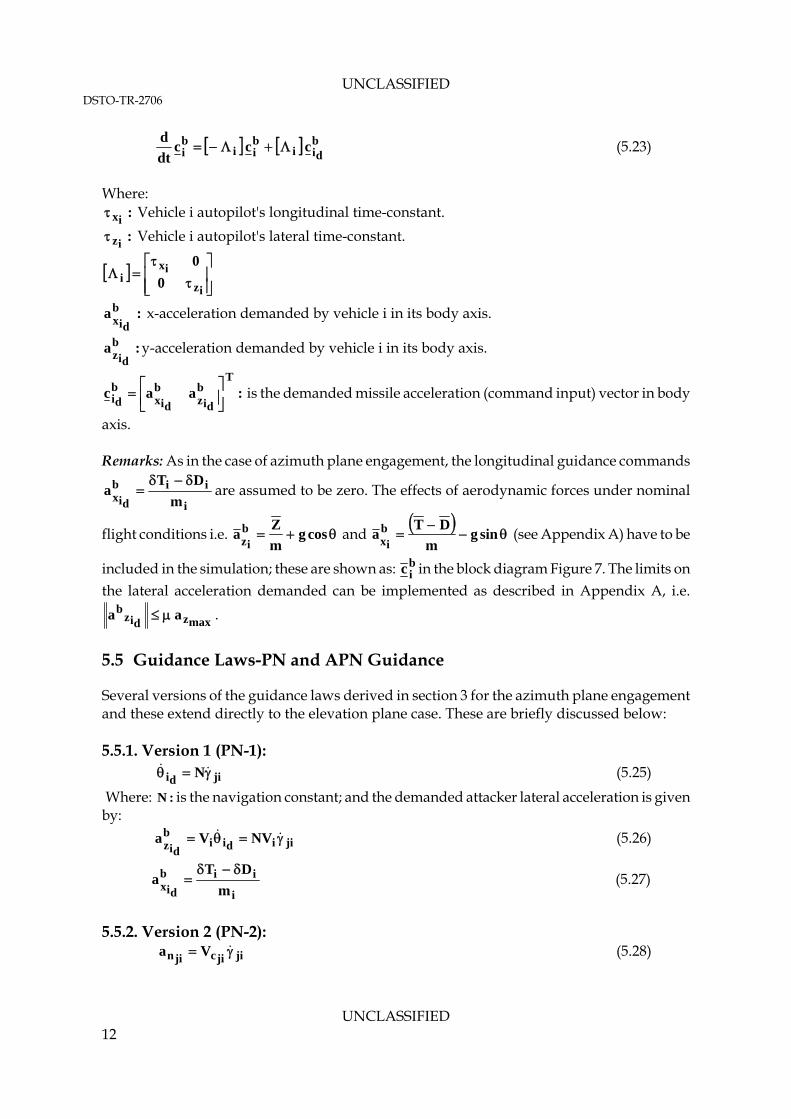
axis. Remarks: As in the case of azimuth plane engagement, the longitudinal guidance commands
i
iib
dix m
DTa
are assumed to be zero. The effects of aerodynamic forces under nominal
flight conditions i.e. cosgm
Zab
iz and
singm
DTab
ix (see Appendix A) have to be
included in the simulation; these are shown as: bic in the block diagram Figure 7. The limits on
the lateral acceleration demanded can be implemented as described in Appendix A, i.e.
maxzdizb aa .
5.5 Guidance Laws-PN and APN Guidance
Several versions of the guidance laws derived in section 3 for the azimuth plane engagement and these extend directly to the elevation plane case. These are briefly discussed below: 5.5.1. Version 1 (PN-1):
jidi N (5.25)
Where: is the navigation constant; and the demanded attacker lateral acceleration is given by:
:N
jiidiib
diz NVVa (5.26)
i
iib
dix m
DTa
(5.27)
5.5.2. Version 2 (PN-2):
jijicjin Va (5.28)
UNCLASSIFIED 12
UNCLASSIFIED DSTO-TR-2706
jijicjinb
diz NVNaa (5.29)
i
iib
dix m
DTa
(5.30)
Where:
:RV jijic is the 'closing velocity' between the attacker and the target.
:ajin is the acceleration normal to the LOS.
5.5.3. Version 3 (PN-3):
jijiijicjiijinb
diz cosNVcosNaa (5.31)
i
iib
dix m
DTa
(5.32)
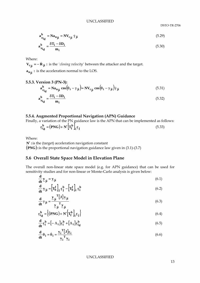
5.5.4. Augmented Proportional Navigation (APN) Guidance Finally, a variation of the PN guidance law is the APN that can be implemented as follows:
jibf
bdi
cTNPNGc (5.33)
Where:
:N is the (target) acceleration navigation constant :PNG is the proportional navigation guidance law given in (3.1)-(3.7) 5.6 Overall State Space Model in Elevation Plane
The overall non-linear state space model (e.g. for APN guidance) that can be used for sensitivity studies and for non-linear or Monte-Carlo analysis is given below:
jijivy
dt
d (6.1)
bii
fb
bjj
fbji cTcTv
dt
d (6.2)
jiT
ji
jiT
jiji
yy
vJy
dt
d (6.3)
jibf
bdi
cTNPNGc (6.4)
bdii
bii
bi ccc
dt
d (6.5)
i
Ti
iT
iii
vv
cJv
dt
d (6.6)
UNCLASSIFIED 13
UNCLASSIFIED DSTO-TR-2706
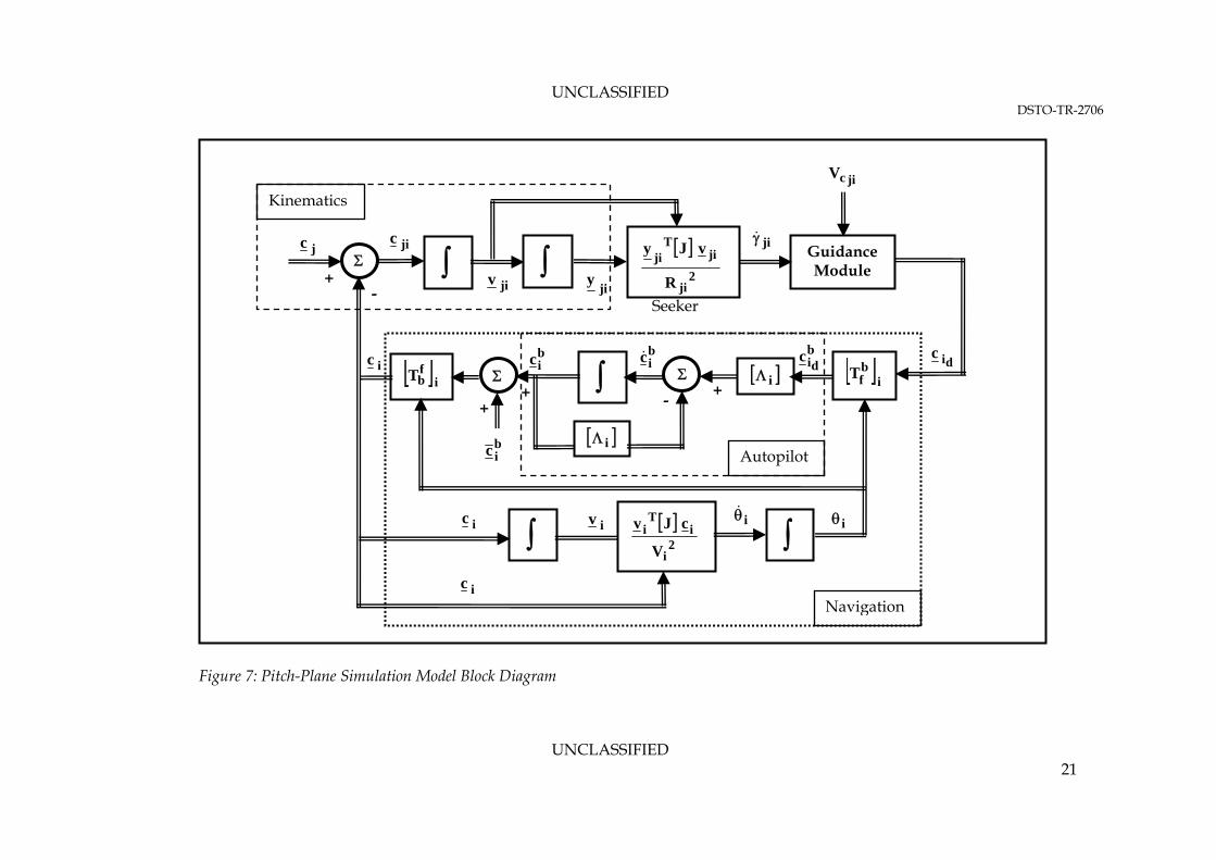
The overall model that can be implemented on the computer is given in Table 5.1. and the block-diagram is shown in Figure 7.
6. Conclusions
In this report mathematical models are derived for multi-vehicle guidance, navigation and control model suitable for developing, implementing and testing modern missile guidance systems. The models allow for incorporating changes in body attitude in addition to autopilot lags, accelerometer limits and aerodynamic effects. These models will be found to be particularly suitable for studying the performance of both the conventional and the modern guidance such as those that arise of game theory and intelligent control theory. The following are considered to be the main contribution of this report:
The models are derived for Az as well as the El plane engagements for multi-vehicle engagement scenarios,
The models incorporate non-linear effects including large changes in vehicle body attitude, autopilot lags, acceleration limits and aerodynamic effects,
The models presented in this report can easily be adapted for multi-run non-linear analysis of guidance performance and for undertaking Monte-Carlo analysis.
7. References
1. Ben-Asher, J.Z., Isaac,Y., Advances in Missile Guidance Theory, Vol. 180 of Progress in Astronautics and Aeronautics, AIAA, 1st ed., 1998. 2. Zarchan, P., Tactical and Strategic Missile Guidance, Vol. 199 of Progress in Astronautics and Aeronautics, AIAA, 2nd ed., 2002. 3. Faruqi F. A., Application of Differential Game Theory to Missile Guidance Problem, DSTO Report (to be published, Dec 2011). 4. Etkin, B.,Lloyd, D.F., Dynamics of Flight, (3rd Ed.), John Wiley & Sons, Inc. New York, 1996.
8. Acknowledgements
The author would like to acknowledge the contribution of Mr. Jim Repo and Mr. Arvind Rajagopalan for their helpful suggestionS and in assisting in the development of computer simulation programming.
UNCLASSIFIED 14

UNCLASSIFIED DSTO-TR-2706
Table 1: Combined (Yaw-Plane) State Space Dynamics Model for Navigation, Seeker, Guidance and Autopilot
ALGORITHM
MODULE NAME
1 ii ux
dt
d
ii audt
d
Kinematics
2
2
1
jiT
jiji xxR
ji
jiT
jijiji R
uxRR
dt
d
jijic RV
2
ji
jiT
jiji
R
uJx
dt
d
jijijiˆ
Seeker
3
1. jiib
dy NVa
2. jijicb
diy NVa
3. jijiijicb
diy cosNVa
4. jibf
bdi
aTNPNGa
Guidance
4 b
diibii
bi aaa
dt
d
Autopilot
5
2
1
iT
ii uuV
2
i
iT
ii
V
aJu
dt
d
ii
iii
fb cossin
sincosT ; T
ibfi
fb TT
bii
fbi aTa
Navigation
UNCLASSIFIED 15
UNCLASSIFIED DSTO-TR-2706
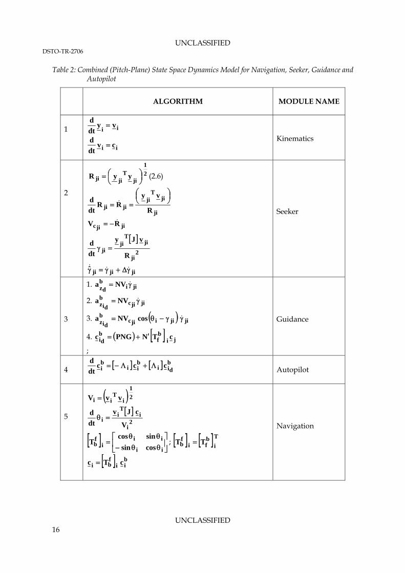
Table 2: Combined (Pitch-Plane) State Space Dynamics Model for Navigation, Seeker, Guidance and Autopilot
ALGORITHM
MODULE NAME
1 ii
vydt
d
ii cvdt
d
Kinematics
2
2
1
jiT
jiji yyR
(2.6)
ji
jiT
jijiji R
vyRR
dt
d
jijic RV
2
ji
jiT
jiji
R
vJy
dt
d
jijijiˆ
Seeker
3
1. jiibdz NVa
2. jijicb
diz NVa
3. jijiijicb
diz cosNVa
4. jibf
bdi
cTNPNGc
;
Guidance
4 b
diibii
bi ccc
dt
d
Autopilot
5
2
1
iT
ii vvV
2
i
iT
ii
V
cJv
dt
d
ii
iii
fb cossin
sincosT ; T
ibfi
fb TT
bii
fbi cTc
Navigation
UNCLASSIFIED 16
UNCLASSIFIED DSTO-TR-2706
Y
2V
X 2x 1x
2y
1y
1V
21R
21na
1
b
d1ya 2
21
Figure 1: Engagement Geometry for 2-Vehicles
iya biya
b
ixa i
i
ixa
Figure 2: Axis transformation fixed <=>body in pitch-plane
UNCLASSIFIED 17
UNCLASSIFIED DSTO-TR-2706
bix
iV i
i
X
Figure 3: Body Incidence
ix
iy
iz
bx
by
bz
Figure 4: Axis System Convention
UNCLASSIFIED 18
UNCLASSIFIED DSTO-TR-2706
UNCLASSIFIED 19
bixa
ixa
iza
biza
i
i
Figure 5: Axis transformation fixed <=>body in pitch-plane
UNCLASSIFIED DSTO-TR-2706
jicV
i
i
i
bfT if
bT
2
i
iT
i
V
aJu
Guidance Module
Kinematics
ji
bia
bdi
a
- +
bia
ia
ia iu
ia
i
ja jia
jiu jix 2ji
jiT
ji
R
uJx
+ -
Seeker
dia
+
bia
+
Autopilot
i
Navigation
Figure 6: Yaw-Plane Simulation Model Block Diagram
UNCLASSIFIED 20
UNCLASSIFIED DSTO-TR-2706
UNCLASSIFIED 21
i
i
i
bfT if
bT
2i
iT
i
V
cJv
Guidance Module
dic
Navigation
jicV
i
bic
bdi
c
Autopilot
ji
i
2
ji
jiT
ji
R
vJy
+
Seeker
-
bic
jiy
iv
Figure 7: Pitch-Plane Simulation Model Block Diagram
+
jiv
bic
+
ic
ic
jic
ic
-
Kinematics
+
jc
UNCLASSIFIED DSTO-TR-2706
Appendix A
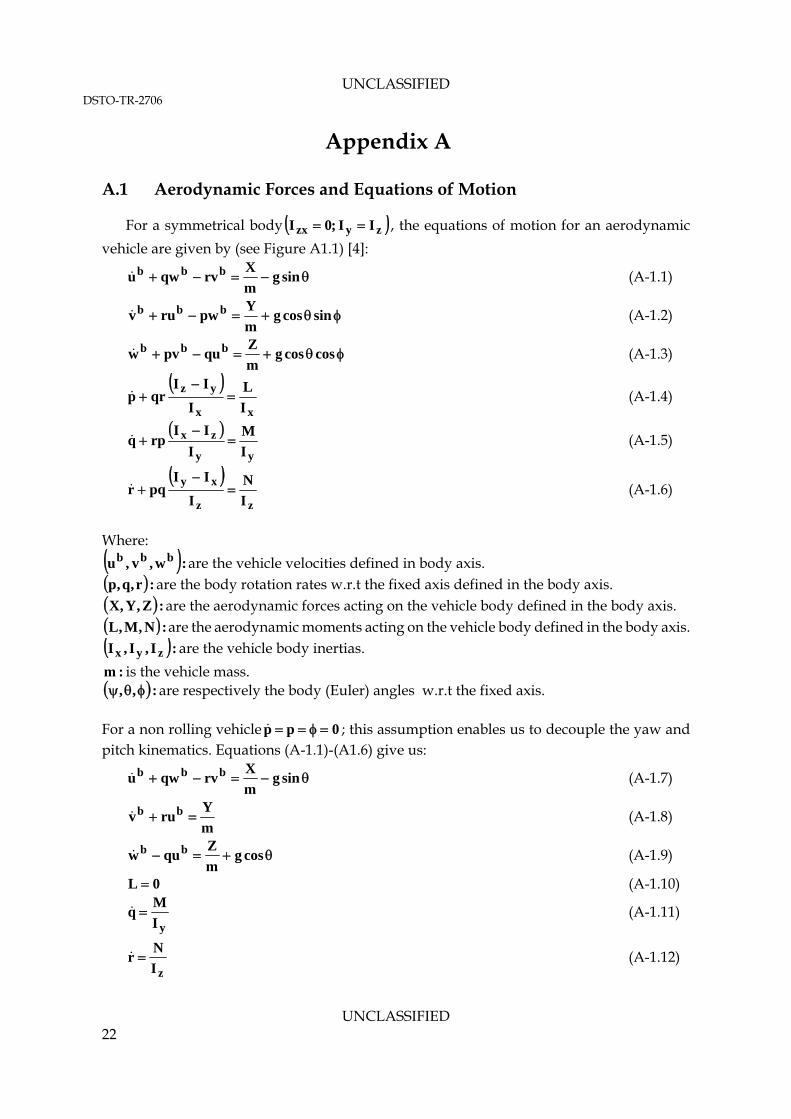
A.1 Aerodynamic Forces and Equations of Motion
For a symmetrical body zyzx II;0I , the equations of motion for an aerodynamic
vehicle are given by (see Figure A1.1) [4]:
singm
Xrvqwu bbb (A-1.1)
sincosgm
Ypwruv bbb (A-1.2)
coscosgm
Zqupvw bbb (A-1.3)
xx
yz
I
L
I
IIqrp
(A-1.4)
yy
zx
I
M
I
IIrpq
(A-1.5)
zz
xy
I
N
I
IIpqr
(A-1.6)
Where:
:w,v,u bbb are the vehicle velocities defined in body axis. :r,q,p are the body rotation rates w.r.t the fixed axis defined in the body axis. :Z,Y,X are the aerodynamic forces acting on the vehicle body defined in the body axis. :N,M,L are the aerodynamic moments acting on the vehicle body defined in the body axis. :I,I,I zyx are the vehicle body inertias.
:m is the vehicle mass. :,, are respectively the body (Euler) angles w.r.t the fixed axis. For a non rolling vehicle ; this assumption enables us to decouple the yaw and pitch kinematics. Equations (A-1.1)-(A1.6) give us:
0pp
singm
Xrvqwu bbb (A-1.7)
m
Yruv bb (A-1.8)
cosgm
Zquw bb (A-1.9)
0L (A-1.10)
yI
Mq (A-1.11)
zI
Nr (A-1.12)
UNCLASSIFIED 22
UNCLASSIFIED DSTO-TR-2706
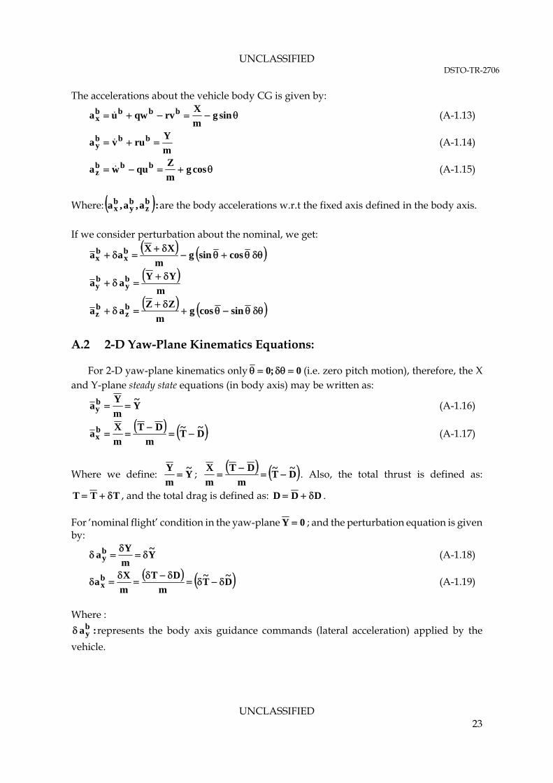
The accelerations about the vehicle body CG is given by:
singm
Xrvqwua bbbb
x (A-1.13)
m
Yruva bbb
y (A-1.14)
cosgm
Zquwa bbb
z (A-1.15)
Where: :a,a,a bz
by
bx are the body accelerations w.r.t the fixed axis defined in the body axis.
If we consider perturbation about the nominal, we get:
cossingm
XXaa b
xbx
m
YYaa b
yby
sincosgm
ZZaa b
zbz
A.2 2-D Yaw-Plane Kinematics Equations:
For 2-D yaw-plane kinematics only 0;0 (i.e. zero pitch motion), therefore, the X and Y-plane steady state equations (in body axis) may be written as:
Y~
m
Yab
y (A-1.16)
D~
T~
m
DT
m
Xab
x
(A-1.17)
Where we define: Y~
m
Y ;
D~
T~
m
DT
m
X
. Also, the total thrust is defined as:
TTT , and the total drag is defined as: DDD . For ‘nominal flight’ condition in the yaw-plane 0Y ; and the perturbation equation is given by:
Y~
m
Yab
y
(A-1.18)
D~
T~
m
DT
m
Xab
x
(A-1.19)
Where :
:aby represents the body axis guidance commands (lateral acceleration) applied by the
vehicle.
UNCLASSIFIED 23
UNCLASSIFIED DSTO-TR-2706
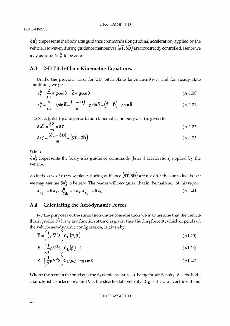
:abx represents the body axis guidance commands (longitudinal acceleration) applied by the
vehicle. However, during guidance manoeuvre D~
,T~ are not directly controlled, Hence we
may assume to be zero. bxa
A.3 2-D Pitch-Plane Kinematics Equations:
Unlike the previous case, for 2-D pitch-plane kinematics 0 , and for steady state conditions, we get:
cosgZ~
cosgm
Zab
z (A-1.20)
singD~
T~
singm
DTsing
m
Xab
x (A-1.21)
The X , Z (pitch)-plane perturbation kinematics (in body axis) is given by:
Z~
m
Zab
z
(A-1.22)
D~
T~
m
DTab
x
(A-1.23)
Where
:abz represents the body axis guidance commands (lateral acceleration) applied by the
vehicle. As in the case of the yaw-plane, during guidance D
~,T
~ are not directly controlled, hence
we may assume to be zero. The reader will recognize, that in the main text of this report: bxa
xb
idx aa , (A-1.24) yb
idy aa zb
idz aa
A.4 Calculating the Aerodynamic Forces
For the purposes of the simulation under consideration we may assume that the vehicle thrust profile tT , say as a function of time, is given; then the drag force D , which depends on the vehicle aerodynamic configuration, is given by:
,CSV
2
1D D
2 (A1.25)
0CSV2
1Y L
2
(A1.26)
cosgCSV
2
1Z L
2 (A1.27)
Where: the term in the bracket is the dynamic pressure; being the air density, is the body
characteristic surface area and
S
V is the steady-state velocity. is the drag coefficient and DC
UNCLASSIFIED 24
UNCLASSIFIED DSTO-TR-2706
UNCLASSIFIED 25
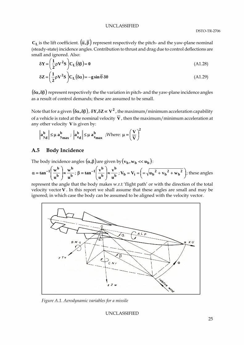
LC is the lift coefficient. , represent respectively the pitch- and the yaw-plane nominal (steady-state) incidence angles. Contribution to thrust and drag due to control deflections are small and ignored. Also:
0CSV2
1Y L
2
(A1.28)
singCSV
2
1Z L
2 (A1.29)
, represent respectively the the variation in pitch- and the yaw-plane incidence angles as a result of control demands; these are assumed to be small.
Note that for a given , , , the maximum/minimum acceleration capability
of a vehicle is rated at the nominal velocity
2VZ,Y
V , then the maximum/minimum acceleration at any other velocity is given by: V
bmaxy
bdy aa ; b
maxzbdz aa ;Where:
2
V
V
A.5 Body Incidence
The body incidence angles are given by, bbb uw,v :
b
b
b
b1
u
w
u
wtan
; b
b
b
b1
u
v
u
vtan
;
2
b2
b2
bib wvuVV ; these angles
represent the angle that the body makes w.r.t ‘flight path’ or with the direction of the total velocity vector . In this report we shall assume that these angles are small and may be ignored; in which case the body can be assumed to be aligned with the velocity vector.
V
Figure A.1. Aerodynamic variables for a missile
Page classification: UNCLASSIFIED
DEFENCE SCIENCE AND TECHNOLOGY ORGANISATION
DOCUMENT CONTROL DATA 1. PRIVACY MARKING/CAVEAT (OF DOCUMENT)
2. TITLE Integrated Navigation, Guidance, and Control of Missile Systems: 2-D Dynamic Models
3. SECURITY CLASSIFICATION (FOR UNCLASSIFIED REPORTS THAT ARE LIMITED RELEASE USE (L) NEXT TO DOCUMENT CLASSIFICATION) Document (U) Title (U) Abstract (U)
4. AUTHOR(S) Farhan A. Faruqi
5. CORPORATE AUTHOR DSTO Defence Science and Technology Organisation PO Box 1500 Edinburgh South Australia 5111 Australia
6a. DSTO NUMBER DSTO-TR-2706
6b. AR NUMBER AR-015-302
6c. TYPE OF REPORT Technical Report
7. DOCUMENT DATE May 2012
8. FILE NUMBER 2012/1001675
9. TASK NUMBER n/a
10. TASK SPONSOR CWSD
11. NO. OF PAGES 19
12. NO. OF REFERENCES 6
DSTO Publications Repository http://dspace.dsto.defence.gov.au/dspace/
14. RELEASE AUTHORITY Chief, Weapons Systems Division
15. SECONDARY RELEASE STATEMENT OF THIS DOCUMENT
Approved for public release OVERSEAS ENQUIRIES OUTSIDE STATED LIMITATIONS SHOULD BE REFERRED THROUGH DOCUMENT EXCHANGE, PO BOX 1500, EDINBURGH, SA 5111 16. DELIBERATE ANNOUNCEMENT No Limitations 17. CITATION IN OTHER DOCUMENTS Yes 18. DSTO RESEARCH LIBRARY THESAURUS Modelling; Missile Guidance; Missile control 19. ABSTRACT In this report mathematical models (2-D Azimuth and Elevation Planes) for multi-party engagement kinematics are derived suitable for developing, implementing and testing modern missile guidance systems. The models developed here are suitable for both conventional and more advanced optimal intelligent guidance schemes including those that arise out of the differential game theory. These models accommodate changes in vehicle body attitude and other non-linear effects such as limits on lateral acceleration and aerodynamic forces.
Page classification: UNCLASSIFIED