integrasi numeris - istiarto.staff.ugm.ac.id integrasi numeris.pdf · fungsi 7 ! fungsi-fungsi yang...
TRANSCRIPT

Numerical Differentiation and Integration
INTEGRASI NUMERIS
http://istiarto.staff.ugm.a.cid
http://istiarto.staff.ugm.ac.id
Integrasi Numeris 2
q Acuan q Chapra, S.C., Canale R.P., 1990, Numerical Methods for Engineers, 2nd
Ed., McGraw-Hill Book Co., New York. n Chapter 15 dan 16, hlm. 459-523.
http://istiarto.staff.ugm.ac.id
Diferensial, Derivatif 3
xi xi +Δx
yi
yi +Δy
Δx
Δy
xi xi +Δx
yi
yi +Δy
xi
yi
(a) (b) (c)
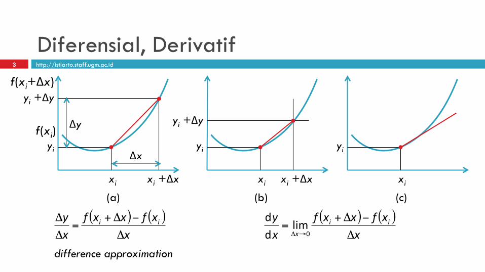
( ) ( )x
xfxxfxy ii
Δ
−Δ+=
Δ
Δ ( ) ( )x
xfxxfxy ii
x Δ
−Δ+=
→Δ 0lim
dd
difference approximation
f(xi+Δx)
f(xi)
http://istiarto.staff.ugm.ac.id
Diferensial, Derivatif 4
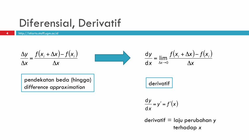
( ) ( )x
xfxxfxy ii
Δ
−Δ+=
Δ
Δ ( ) ( )x
xfxxfxy ii
x Δ
−Δ+=
→Δ 0lim
dd
pendekatan beda (hingga) difference approximation derivatif
( )xfyxy
ʹ′=ʹ′=dd
derivatif = laju perubahan y terhadap x
http://istiarto.staff.ugm.ac.id
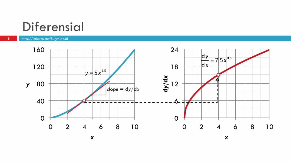
Diferensial
0
40
80
120
160
0 2 4 6 8 10
y
x
slope = dy/dx
0
6
12
18
24
0 2 4 6 8 10
dy/d
x
x
5
5.15xy =
5.05.7dd xxy=
http://istiarto.staff.ugm.ac.id
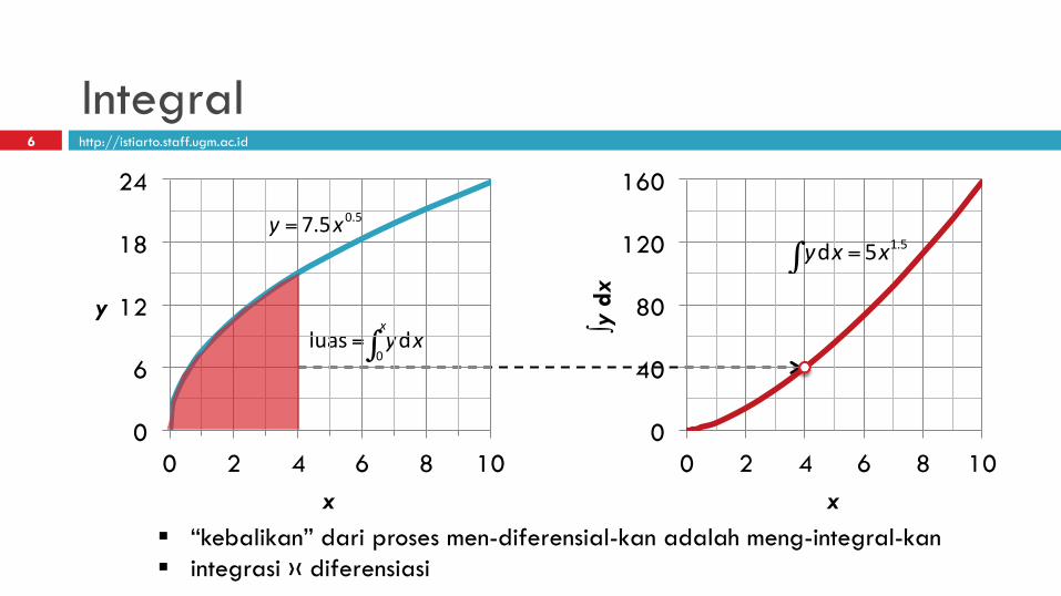
Integral
0
40
80
120
160
0 2 4 6 8 10
∫y d
x
x
6
5.05.7 xy =5.15d xxy =∫
∫=x
xy0dluas
§ “kebalikan” dari proses men-diferensial-kan adalah meng-integral-kan § integrasi ›‹ diferensiasi
0
6
12
18
24
0 2 4 6 8 10
y
x
http://istiarto.staff.ugm.ac.id
Fungsi 7
q Fungsi-fungsi yang di-diferensial-kan atau di-integral-kan dapat berupa: q fungsi kontinu sederhana: polinomial, eksponensial, trigonometri
q fungsi kontinu kompleks yang tidak memungkinkan didiferensialkan atau dintegralkan secara langsung
q fungsi yang nilai-nilainya disajikan dalam bentuk tabel [tabulasi data x vs f(x)]

http://istiarto.staff.ugm.ac.id
Cara mencari nilai integral 8
( )∫ +
++2
0
5.023
dsin5.01
1cos2 xex
x x
x f(x)
0.25 2.599
0.75 2.414
1.25 1.945
1.75 1.993 0
1
2
3
4
0 0.5 1 1.5 2 2.5
A1 A2 A3 A4
∫f(x) dx = luas = ∑Ai
http://istiarto.staff.ugm.ac.id
Derivatif 9
xuun
xy n
dd
dd 1−=
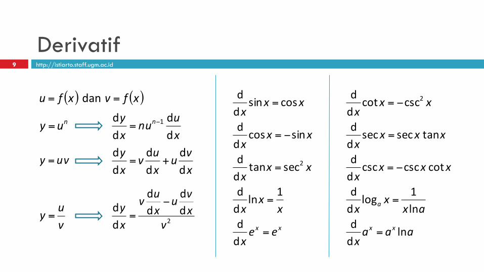
( ) ( )xfvxfu == dan
nuy =
vuy =
vuy =
xvu
xuv
xy
dd
dd
dd
+=
2dd
dd
dd
vxvu
xuv
xy −=
xx eex
xx
x
xxx
xxx
xxx
=
=
=
−=
=
dd
1lndd
sectandd
sincosdd
cossindd
2
aaax
axx
x
xxxx
xxxx
xxx
xx
a
lndd
ln1log
dd
cotcsccscdd
tansecsecdd
csccotdd 2
=
=
−=
=
−=
http://istiarto.staff.ugm.ac.id
Integral 10
( ) ( ) Cbaxa
xbax
Cxxx
aaCab
axa
nCnuvu
uvuvvu
bxbx
nn
++−=+
+=
≠>+=
−≠++
=
−=
∫
∫
∫
∫
∫∫+
cos1dsin
lnd
1,0ln
d
11
d
dd1
( ) ( )
( )
Cxaab
abbxax
Caxaexex
Caexe
Cxxxxx
Cbaxa
xbax
axax
axax
+=+
+−=
+=
+−=
++=+
−∫
∫
∫
∫
∫
12
2
tan1d
1d
d
lndln
sin1dcos
Metode Trapesium Metode Simpson Metode Kuadratur Gauss
Metode Integrasi Newton-Cotes 11
http://istiarto.staff.ugm.ac.id
http://istiarto.staff.ugm.ac.id
Persamaan Newton-Cotes 12
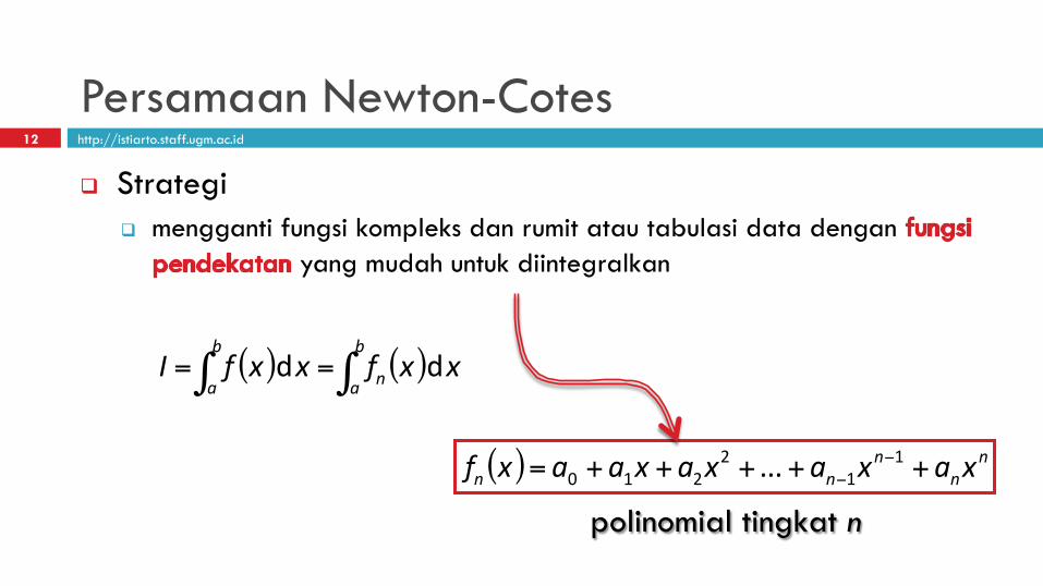
q Strategi q mengganti fungsi kompleks dan rumit atau tabulasi data dengan
yang mudah untuk diintegralkan
( ) ( )∫∫ ==b
a n
b
axxfxxfI dd
( ) nn
nnn xaxaxaxaaxf +++++= −−
11
2210 ...
polinomial tingkat n
http://istiarto.staff.ugm.ac.id
Persamaan Newton-Cotes 13
( )xf
x a b
( )xf
x a b
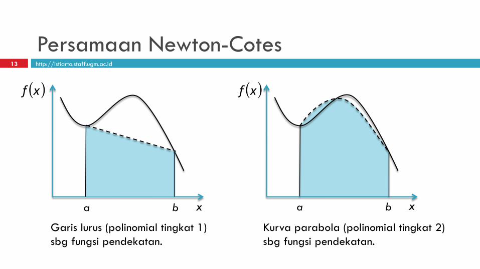
Garis lurus (polinomial tingkat 1) sbg fungsi pendekatan.
Kurva parabola (polinomial tingkat 2) sbg fungsi pendekatan.
http://istiarto.staff.ugm.ac.id
Persamaan Newton-Cotes 14
( )xf
x a b
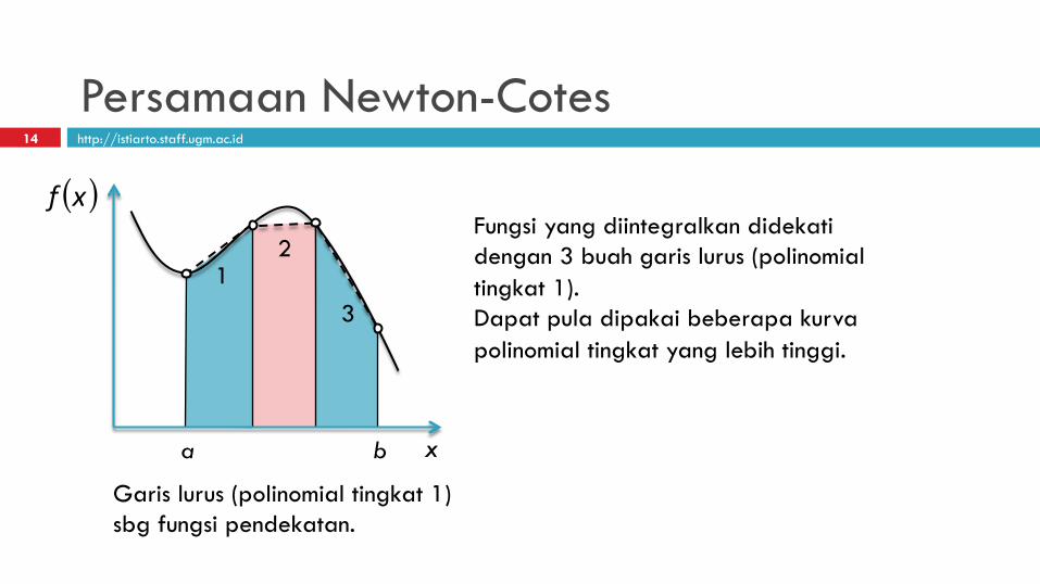
Garis lurus (polinomial tingkat 1) sbg fungsi pendekatan.
1 2
3
Fungsi yang diintegralkan didekati dengan 3 buah garis lurus (polinomial tingkat 1). Dapat pula dipakai beberapa kurva polinomial tingkat yang lebih tinggi.
http://istiarto.staff.ugm.ac.id
Metode Trapesium 15
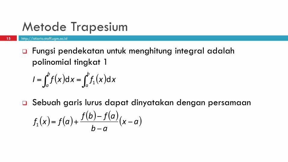
q Fungsi pendekatan untuk menghitung integral adalah polinomial tingkat 1
q Sebuah garis lurus dapat dinyatakan dengan persamaan
( ) ( )∫∫ ==b
a
b
axxfxxfI dd 1
( ) ( ) ( ) ( )( )axabafbfafxf −
−
−+=1
http://istiarto.staff.ugm.ac.id
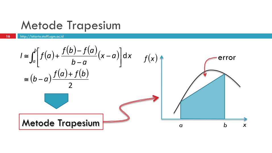
Metode Trapesium 16
( ) ( ) ( )( )
( ) ( ) ( )2
d
bfafab
xaxabafbfafI
b
a
+−≅
⎥⎦⎤
⎢⎣⎡ −
−
−+≅ ∫
Metode Trapesium
( )xf
x a b
error
http://istiarto.staff.ugm.ac.id
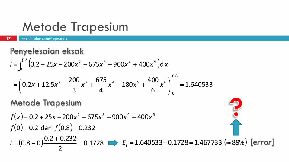
Metode Trapesium 17
( )
640533.16400180
4675
32005.122.0
d400900675200252.08.0
0
65432
8.0
0
5432
=⎟⎠⎞
⎜⎝⎛ +−+−+=
+−+−+= ∫
xxxxxx
xxxxxxI
( )( ) ( ) 232.08.0 dan 2.00
400900675200252.0 5432
==
+−+−+=
ffxxxxxxf
Penyelesaian eksak
Metode Trapesium
( ) 1728.02232.02.008.0 =
+−=I [error] ( )%89467733.11728.0640533.1 ≈=−=tE
http://istiarto.staff.ugm.ac.id
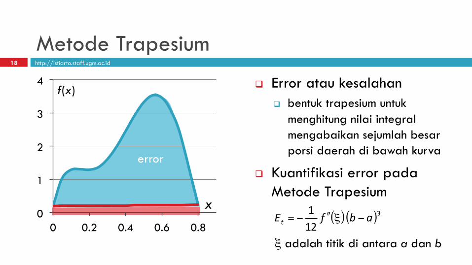
0
1
2
3
4
0 0.2 0.4 0.6 0.8
x
f(x)
Metode Trapesium
q Error atau kesalahan q bentuk trapesium untuk
menghitung nilai integral mengabaikan sejumlah besar porsi daerah di bawah kurva
q Kuantifikasi error pada Metode Trapesium
18
error
( )( )3121 abfEt −ξʹ′ʹ′−=
ξ adalah titik di antara a dan b
http://istiarto.staff.ugm.ac.id
Metode Trapesium
0
1
2
3
4
0 0.2 0.4 0.6 0.8
x
f(x)
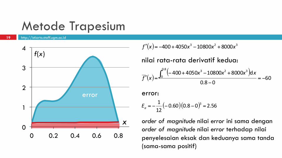
19
error ( )( ) 56.208.060.0
121 3 =−−−=aE
( ) 323 8000108004050400 xxxxf +−+−=ʹ′ʹ′
nilai rata-rata derivatif kedua:
( )( )
6008.0
d80001080040504008.0
0
323
−=−
+−+−=ʹ′ʹ′ ∫ xxxx
xf
error:
order of magnitude nilai error ini sama dengan order of magnitude nilai error terhadap nilai penyelesaian eksak dan keduanya sama tanda (sama-sama positif)
http://istiarto.staff.ugm.ac.id
Trapesium multi pias 20
q Peningkatan akurasi q selang ab dibagi menjadi sejumlah n pias dengan lebar seragam h
nabh −
=
http://istiarto.staff.ugm.ac.id
0
1
2
3
4
0 0.1 0.2 0.3 0.4 0.5 0.6 0.7 0.8
x
f(x)
h = 0.1
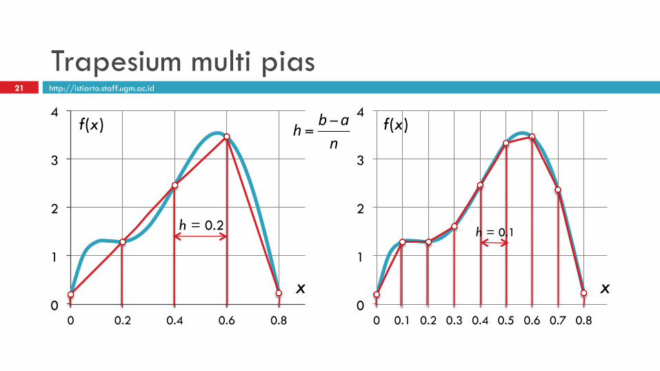
Trapesium multi pias
0
1
2
3
4
0 0.2 0.4 0.6 0.8
x
f(x)
h = 0.2
21
nabh −
=
http://istiarto.staff.ugm.ac.id
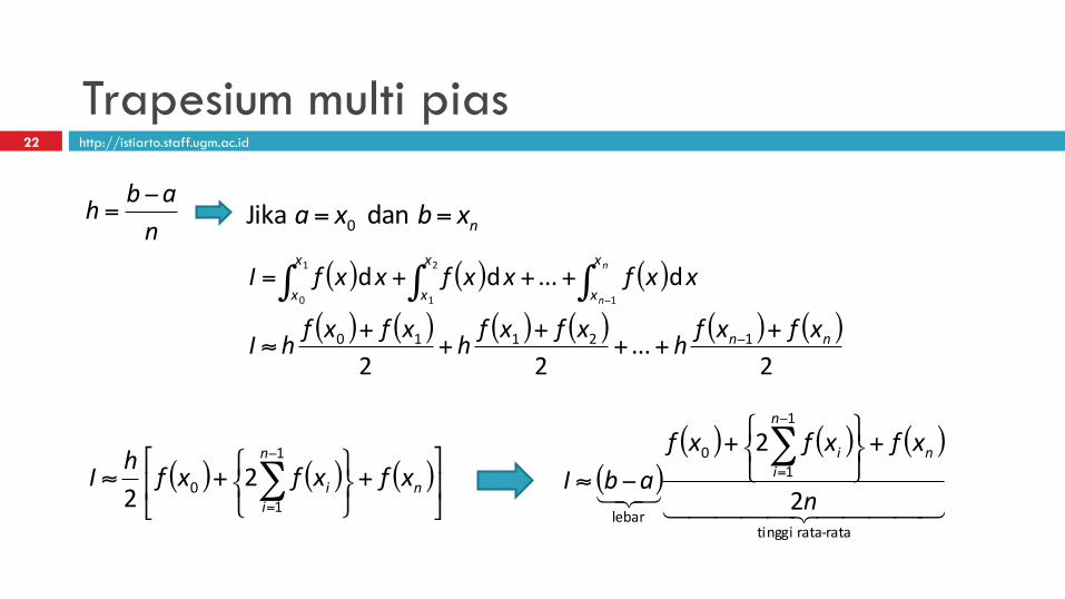
Trapesium multi pias 22
nabh −
=nxbxa == dan Jika 0
( ) ( ) ( )
( ) ( ) ( ) ( ) ( ) ( )2
...22
d...dd
12110
1
2
1
1
0
nn
x
x
x
x
x
x
xfxfhxfxfhxfxfhI
xxfxxfxxfI n
n
+++
++
+≈
+++=
−
∫∫∫−
( ) ( ) ( )⎥⎦
⎤⎢⎣
⎡+
⎭⎬⎫
⎩⎨⎧
+≈ ∑−
=n
n
ii xfxfxfhI
1
10 2
2( )
( ) ( ) ( )
!!!! "!!!! #$"#$rata-‐rata tinggi
1
10
lebar2
2
n
xfxfxfabI
n
n
ii +⎭⎬⎫
⎩⎨⎧
+−≈
∑−
=
http://istiarto.staff.ugm.ac.id
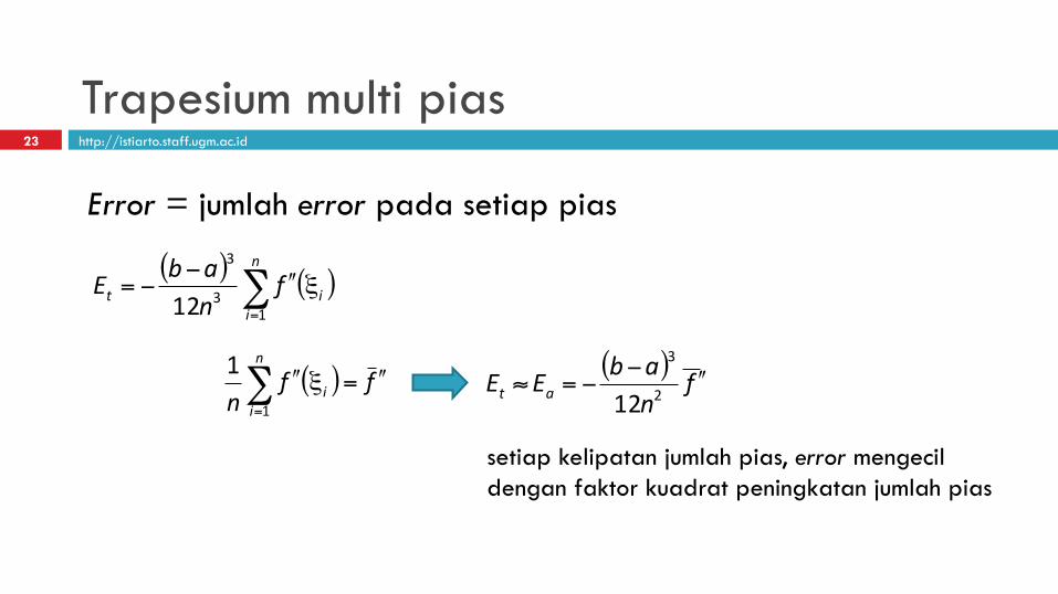
Trapesium multi pias 23
( ) ( )∑=
ξʹ′ʹ′−
−=n
iit f
nabE
13
3
12
Error = jumlah error pada setiap pias
( ) ffn
n
ii ʹ′ʹ′=ξʹ′ʹ′∑
=1
1 ( ) fnabEE at ʹ′ʹ′−
−=≈ 2
3
12
setiap kelipatan jumlah pias, error mengecil dengan faktor kuadrat peningkatan jumlah pias
http://istiarto.staff.ugm.ac.id
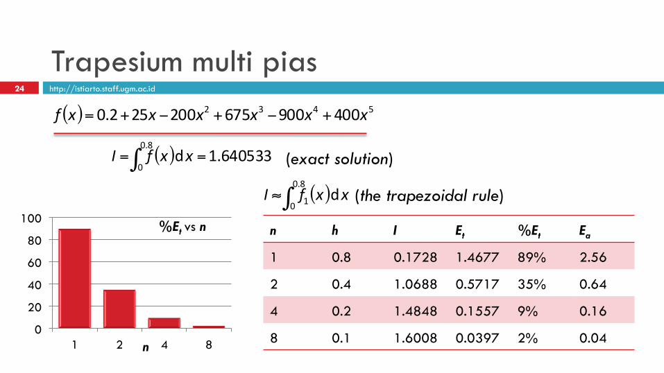
Trapesium multi pias 24
( ) 5432 400900675200252.0 xxxxxxf +−+−+=
n h I Et %Et Ea
1 0.8 0.1728 1.4677 89% 2.56
2 0.4 1.0688 0.5717 35% 0.64
4 0.2 1.4848 0.1557 9% 0.16
8 0.1 1.6008 0.0397 2% 0.04
( ) 640533.1d8.0
0== ∫ xxfI
( )∫≈8.0
0 1 dxxfI (the trapezoidal rule)
(exact solution)
0
20
40
60
80
100
1 2 4 8 n
%Et vs n

http://istiarto.staff.ugm.ac.id
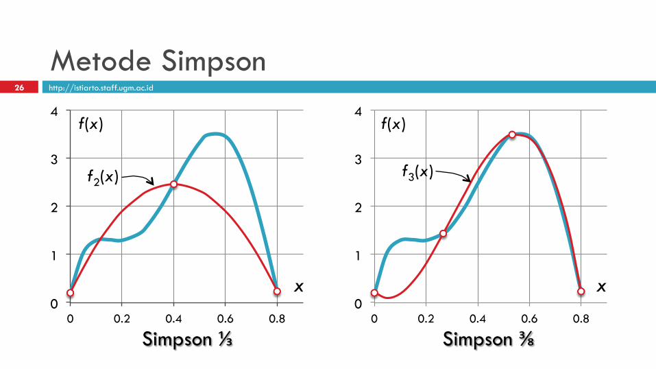
Metode Simpson
q Fungsi pendekatan: polinomial tingkat 1 q Peningkatan ketelitian dpt
dilakukan dengan meningkatkan jumlah pias
q Fungsi pendekatan: polinomial: q tingkat 2: Simpson 1/3
q tingkat 3: Simpson 3/8
25
The trapezoidal rule Simpson’s rules
http://istiarto.staff.ugm.ac.id
Metode Simpson
0
1
2
3
4
0 0.2 0.4 0.6 0.8
x
f(x)
f2(x)
0
1
2
3
4
0 0.2 0.4 0.6 0.8
x
f(x)
f3(x)
26
Simpson ⅓ Simpson ⅜
http://istiarto.staff.ugm.ac.id
Metode Simpson 27
q Polinomial tingkat 2 atau 3 q dicari dengan Metode Newton atau Lagrange (lihat materi tentang
curve fitting)
http://istiarto.staff.ugm.ac.id
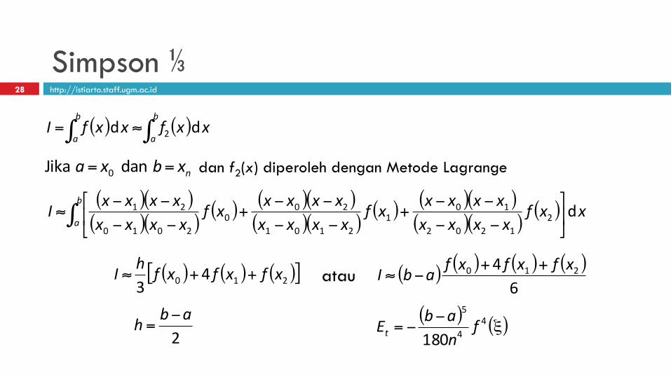
Simpson ⅓ 28
( ) ( )∫∫ ≈=b
a
b
axxfxxfI dd 2
nxbxa == dan Jika 0
( )( )( )( )
( ) ( )( )( )( )
( ) ( )( )( )( )
( )∫ ⎥⎦
⎤⎢⎣
⎡
−−−−
+−−−−
+−−−−
≈b
axxf
xxxxxxxxxf
xxxxxxxxxf
xxxxxxxxI d2
1202
101
2101
200
2010
21
dan f2(x) diperoleh dengan Metode Lagrange
( ) ( ) ( )[ ]210 43
xfxfxfhI ++≈
2abh −
=
( ) ( ) ( ) ( )6
4 210 xfxfxfabI ++−≈atau
( ) ( )ξ−−= 4
4
5
180f
nabEt
http://istiarto.staff.ugm.ac.id
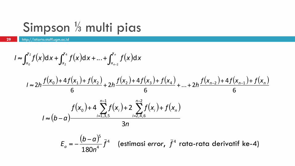
Simpson ⅓ multi pias 29
( ) ( ) ( )∫∫∫−
+++≈n
n
x
x
x
x
x
xxxfxxfxxfI
2
4
2
2
0
d...dd
( ) ( ) ( ) ( ) ( ) ( ) ( ) ( ) ( )6
42...
64
26
42 12432210 nnn xfxfxf
hxfxfxf
hxfxfxf
hI++
++++
+++
≈ −−
( )( ) ( ) ( ) ( )
n
xfxfxfxfabI
n
n
ii
n
ii
3
242
6,4,2
1
5,3,10 +++
−≈∑∑−
=
−
=
( ) 44
5
180f
nabEa
−−= (estimasi error, 4f rata-rata derivatif ke-4)
http://istiarto.staff.ugm.ac.id
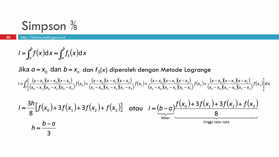
Simpson ⅜ 30
( ) ( )∫∫ ≈=b
a
b
axxfxxfI dd 3
nxbxa == dan Jika 0
( )( )( )( )( )( )
( ) ( )( )( )( )( )( )
( ) ( )( )( )( )( )( )
( ) ( )( )( )( )( )( )
( )∫ ⎥⎦
⎤⎢⎣
⎡
−−−−−−
+−−−−−−
+−−−−−−
+−−−−−−
≈b
axxf
xxxxxxxxxxxxxf
xxxxxxxxxxxxxf
xxxxxxxxxxxxxf
xxxxxxxxxxxxI d3
231303
2102
321202
3101
312101
3200
302010
321
dan f3(x) diperoleh dengan Metode Lagrange
( ) ( ) ( ) ( )[ ]3210 3383 xfxfxfxfhI +++≈
3abh −
=
( ) ( ) ( ) ( ) ( )!!!!! "!!!!! #$"#$
ratarata tinggi
3210
lebar833
−
+++−≈
xfxfxfxfabIatau
http://istiarto.staff.ugm.ac.id
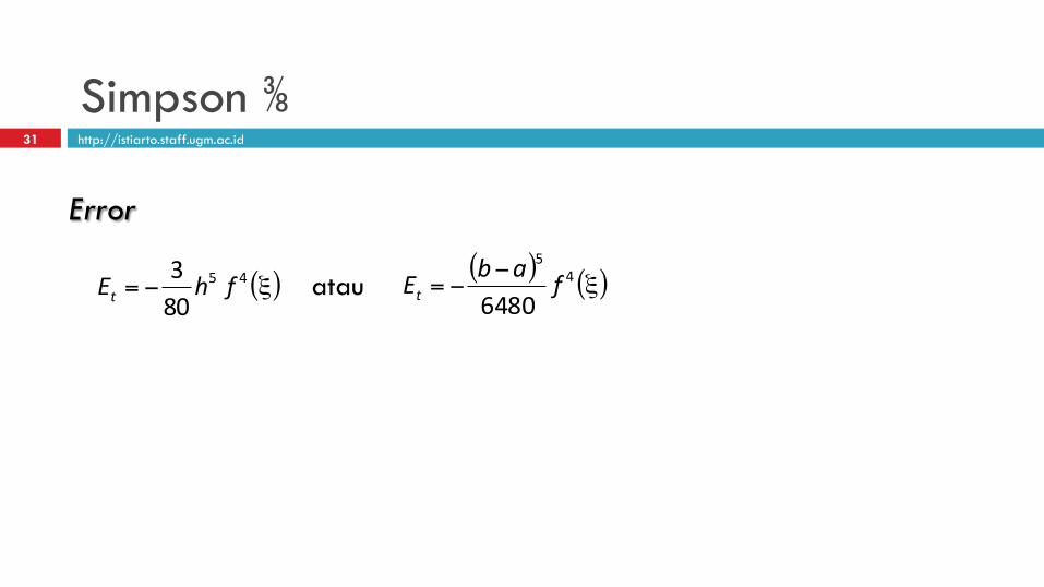
Simpson ⅜ 31
( ) ( )ξ−−= 4
5
6480fabEt
Error
( )ξ−= 45
803 fhEt atau
http://istiarto.staff.ugm.ac.id
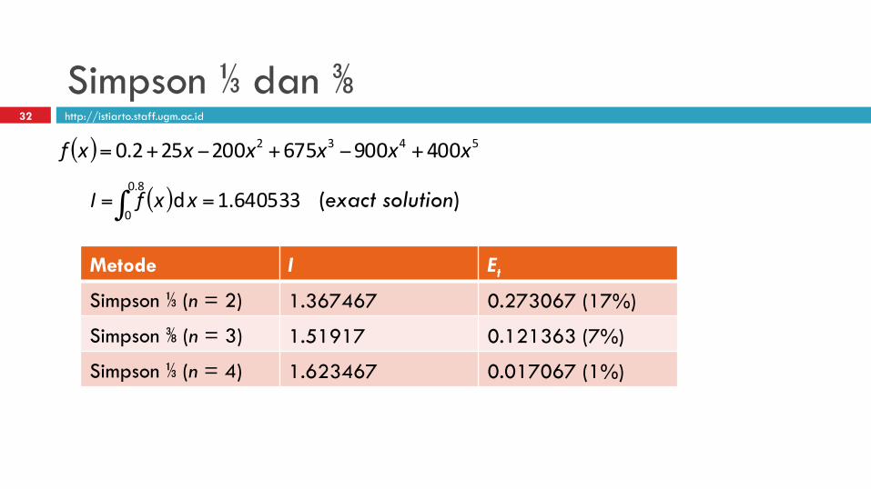
Simpson ⅓ dan ⅜ 32
( ) 5432 400900675200252.0 xxxxxxf +−+−+=
( ) 640533.1d8.0
0== ∫ xxfI (exact solution)
Metode I Et
Simpson ⅓ (n = 2) 1.367467 0.273067 (17%)
Simpson ⅜ (n = 3) 1.51917 0.121363 (7%)
Simpson ⅓ (n = 4) 1.623467 0.017067 (1%)
http://istiarto.staff.ugm.ac.id
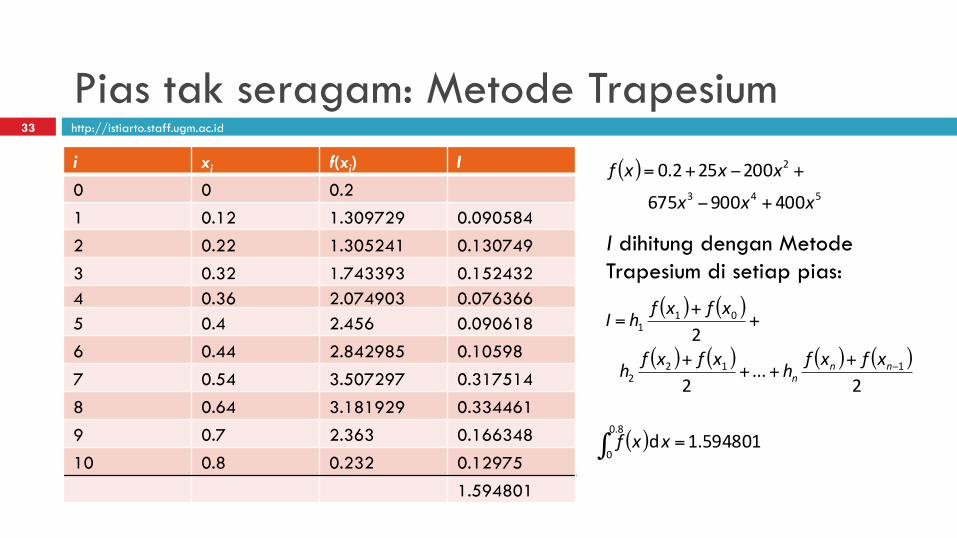
Pias tak seragam: Metode Trapesium 33
( )543
2
400900675
200252.0
xxx
xxxf
+−
+−+=i xi f(xi) I
0 0 0.2
1 0.12 1.309729 0.090584
2 0.22 1.305241 0.130749
3 0.32 1.743393 0.152432 4 0.36 2.074903 0.076366 5 0.4 2.456 0.090618
6 0.44 2.842985 0.10598
7 0.54 3.507297 0.317514
8 0.64 3.181929 0.334461
9 0.7 2.363 0.166348
10 0.8 0.232 0.12975
1.594801
I dihitung dengan Metode Trapesium di setiap pias:
( ) ( )
( ) ( ) ( ) ( )2
...2
2112
2
011
−+++
+
++
=
nnn
xfxfhxfxfh
xfxfhI
( ) 594801.1d8.0
0=∫ xxf
http://istiarto.staff.ugm.ac.id
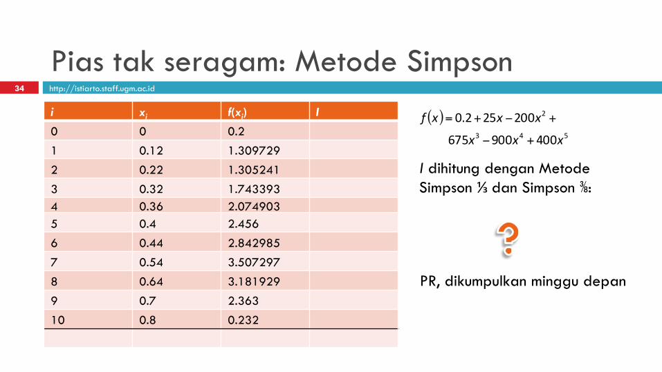
Pias tak seragam: Metode Simpson 34
( )543
2
400900675
200252.0
xxx
xxxf
+−
+−+=i xi f(xi) I
0 0 0.2
1 0.12 1.309729
2 0.22 1.305241
3 0.32 1.743393 4 0.36 2.074903 5 0.4 2.456
6 0.44 2.842985
7 0.54 3.507297
8 0.64 3.181929
9 0.7 2.363
10 0.8 0.232
I dihitung dengan Metode Simpson ⅓ dan Simpson ⅜:
PR, dikumpulkan minggu depan
http://istiarto.staff.ugm.ac.id
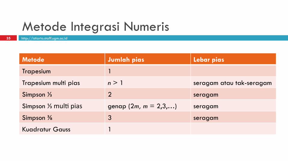
Metode Integrasi Numeris 35
Metode Jumlah pias Lebar pias
Trapesium 1
Trapesium multi pias n > 1 seragam atau tak-seragam
Simpson ⅓ 2 seragam
Simpson ⅓ mul( pias genap (2m, m = 2,3,…) seragam
Simpson ⅜ 3 seragam
Kuadratur Gauss 1
http://istiarto.staff.ugm.ac.id
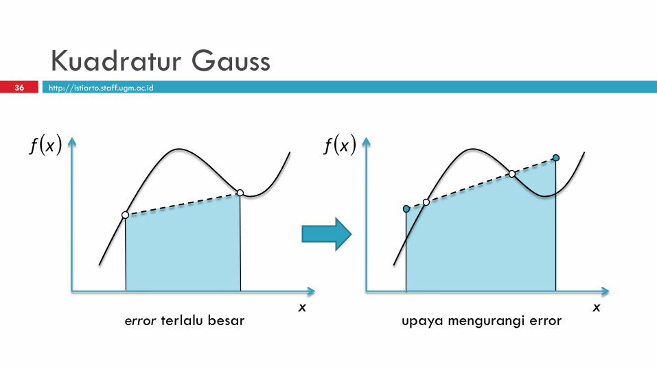
Kuadratur Gauss 36
( )xf
x
( )xf
x error terlalu besar upaya mengurangi error
http://istiarto.staff.ugm.ac.id
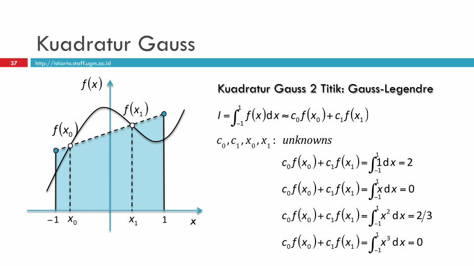
Kuadratur Gauss 37
( )xf
x
( )0xf
( )1xf
0x 1x1− 1
Kuadratur Gauss 2 Titik: Gauss-Legendre
( ) ( ) ( )1100
1
1d xfcxfcxxfI +≈= ∫−
( ) ( )
( ) ( )
( ) ( )
( ) ( ) 0d
32d
0d
2d1
1
1
31100
1
1
21100
1
11100
1
11100
==+
==+
==+
==+
∫
∫
∫
∫
−
−
−
−
xxxfcxfc
xxxfcxfc
xxxfcxfc
xxfcxfc!!c0 ,c1 , x0 , x1 : !!unknowns
http://istiarto.staff.ugm.ac.id
0
0.5
1
1.5
2
-1.5 -1 -0.5 0 0.5 1 1.5 -1.5
-1
-0.5
0
0.5
1
1.5
-1.5 -1 -0.5 0 0.5 1 1.5
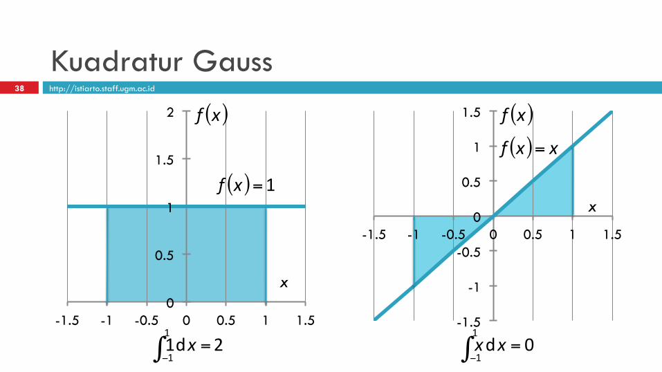
Kuadratur Gauss 38
( )xf
x
( ) 1=xf
( ) xxf =
2d11
1=∫− x 0d
1
1=∫− xx
( )xf
x
http://istiarto.staff.ugm.ac.id
0
1
2
-1.5 -1 -0.5 0 0.5 1 1.5
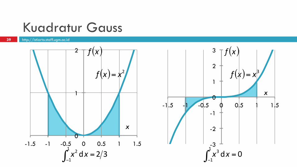
Kuadratur Gauss 39
( )xf
x
( ) 2xxf = ( ) 3xxf =
32d1
1
2 =∫− xx 0d1
1
3 =∫− xx
( )xf
x
-3
-2
-1
0
1
2
3
-1.5 -1 -0.5 0 0.5 1 1.5
http://istiarto.staff.ugm.ac.id
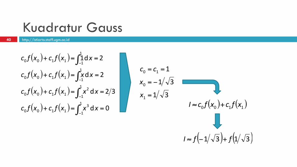
Kuadratur Gauss 40
( ) ( )
( ) ( )
( ) ( )
( ) ( ) 0d
32d
2d
2d1
1
1
31100
1
1
21100
1
11100
1
11100
==+
==+
==+
==+
∫
∫
∫
∫
−
−
−
−
xxxfcxfc
xxxfcxfc
xxxfcxfc
xxfcxfc
( ) ( )1100 xfcxfcI +≈31
31
1
1
0
10
=
−=
==
x
x
cc
( ) ( )3131 ffI +−≈
http://istiarto.staff.ugm.ac.id
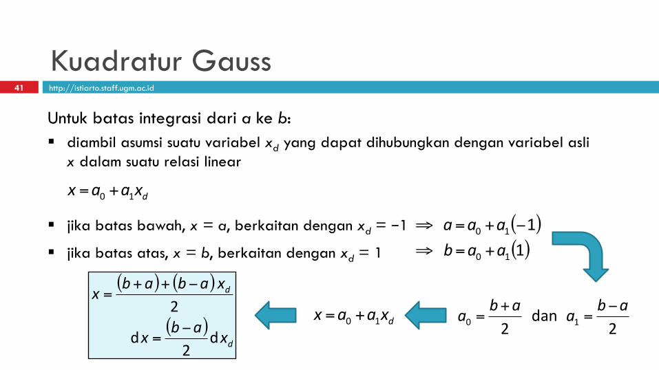
Kuadratur Gauss 41
Untuk batas integrasi dari a ke b: § diambil asumsi suatu variabel xd yang dapat dihubungkan dengan variabel asli
x dalam suatu relasi linear
dxaax 10 +=
§ jika batas bawah, x = a, berkaitan dengan xd = −1
§ jika batas atas, x = b, berkaitan dengan xd = 1
( )110 −+=⇒ aaa( )110 aab +=⇒
2 dan
2 10abaaba −
=+
=
( ) ( )
( )d
d
xabx
xababx
d2
d
2−
=
−++=
dxaax 10 +=
http://istiarto.staff.ugm.ac.id
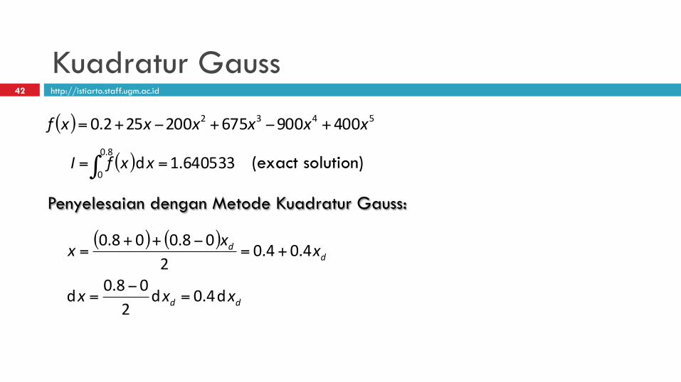
Kuadratur Gauss 42
( ) 5432 400900675200252.0 xxxxxxf +−+−+=
( ) 640533.1d8.0
0== ∫ xxfI (exact solution)
Penyelesaian dengan Metode Kuadratur Gauss:
( ) ( )
dd
dd
xxx
xxx
d4.0d2
08.0d
4.04.02
08.008.0
=−
=
+=−++
=
http://istiarto.staff.ugm.ac.id
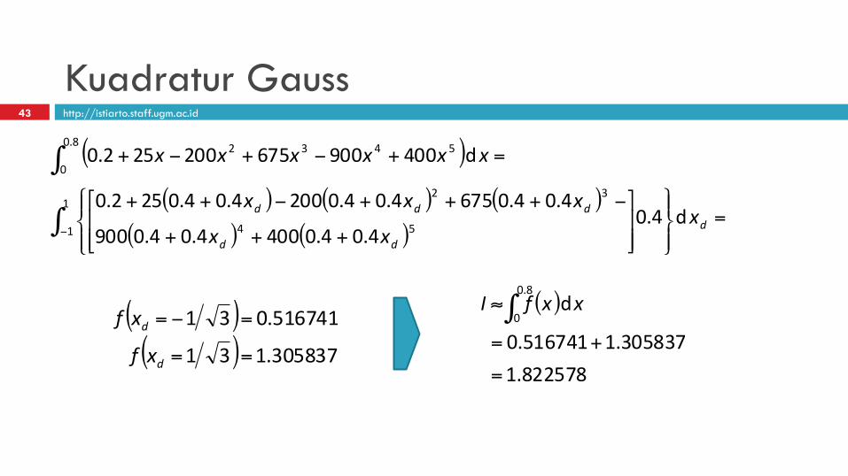
Kuadratur Gauss 43
( )( ) ( ) ( )
( ) ( )=
⎪⎭
⎪⎬⎫
⎪⎩
⎪⎨⎧
⎥⎥⎦
⎤
⎢⎢⎣
⎡
+++
−+++−++
=+−+−+
∫
∫
−
1
1 54
32
8.0
0
5432
d4.04.04.04004.04.0900
4.04.06754.04.02004.04.0252.0
d400900675200252.0
ddd
ddd xxx
xxx
xxxxxx
( )( ) 305837.131
516741.031
==
=−=
d
d
xf
xf( )
822578.1305837.1516741.0
d8.0
0
=
+=
≈ ∫ xxfI

44 http://istiarto.staff.ugm.ac.id