integral calculus with applications to the life sciences · ii leah edelstein-keshet list of...
TRANSCRIPT
Integral Calculus with Applications to theLife Sciences
Leah Edelstein-Keshet
Mathematics Department, University of British Columbia, Vancouver
November 21, 2017
Course Notes for Mathematics 103c© Leah Keshet. Not to be copied, used, distributed or revised
without explicit written permission from the copyright owner.

ii Leah Edelstein-Keshet
List of ContributorsLeah Edelstein-Keshet Department of Mathematics, UBC, Vancouver
Author of course notes.
Justin Martel Department of Mathematics, UBC, VancouverWrote and extended chapters on sequences, series and improper integrals – January2013.
Christoph Hauert Department of Mathematics, UBC, VancouverEdited, restructured and extended chapters on sequences, series and improper inte-grals; wrote section on difference equations and the logistic map; new figures forchapters on sequences, series and improper integrals – February-April 2013.Corrections & inclusion of problems sets – November-December 2014
Wes Maciejewski Department of Mathematics, UBC, VancouverVaccination example, Section 4.6 – April 2013.
Contents
Preface xvii
1 Areas, volumes and simple sums 11.1 Introduction . . . . . . . . . . . . . . . . . . . . . . . . . . . . . . . 11.2 Areas of simple shapes . . . . . . . . . . . . . . . . . . . . . . . . . 1
1.2.1 Example 1: Finding the area of a polygon using triangles:a “dissection” method . . . . . . . . . . . . . . . . . . . 3
1.2.2 Example 2: How Archimedes discovered the area of acircle: dissect and “take a limit” . . . . . . . . . . . . . . 4
1.3 Simple volumes . . . . . . . . . . . . . . . . . . . . . . . . . . . . . 61.3.1 Example 3: The Tower of Hanoi: a tower of disks . . . . 8
1.4 Sigma Notation . . . . . . . . . . . . . . . . . . . . . . . . . . . . . 91.4.1 Formulae for sums of integers, squares, and cubes . . . . 12
1.5 Summing the geometric series . . . . . . . . . . . . . . . . . . . . . . 151.6 Prelude to infinite series . . . . . . . . . . . . . . . . . . . . . . . . . 16
1.6.1 The infinite geometric series . . . . . . . . . . . . . . . . 161.6.2 Example: A geometric series that converges. . . . . . . . 181.6.3 Example: A geometric series that diverges . . . . . . . . 18
1.7 Application of geometric series to the branching structure of the lungs 181.7.1 Assumptions . . . . . . . . . . . . . . . . . . . . . . . . 191.7.2 A simple geometric rule . . . . . . . . . . . . . . . . . . 211.7.3 Total number of segments . . . . . . . . . . . . . . . . . 221.7.4 Total volume of airways in the lung . . . . . . . . . . . . 221.7.5 Total surface area of the lung branches . . . . . . . . . . 231.7.6 Summary of predictions for specific parameter values . . 241.7.7 Exploring the problem numerically . . . . . . . . . . . . 251.7.8 For further independent study . . . . . . . . . . . . . . . 25
1.8 Summary . . . . . . . . . . . . . . . . . . . . . . . . . . . . . . . . . 271.9 Optional Material . . . . . . . . . . . . . . . . . . . . . . . . . . . . 29
1.9.1 How to prove the formulae for sums of squares and cubes 291.10 Exercises . . . . . . . . . . . . . . . . . . . . . . . . . . . . . . . . . 31
2 Areas 392.1 Areas in the plane . . . . . . . . . . . . . . . . . . . . . . . . . . . . 39
iii
iv Contents
2.2 Computing the area under a curve by rectangular strips . . . . . . . . 412.2.1 First approach: Numerical integration using a spreadsheet 412.2.2 Second approach: Analytic computation using Riemann
sums . . . . . . . . . . . . . . . . . . . . . . . . . . . . 422.2.3 Comments . . . . . . . . . . . . . . . . . . . . . . . . . 45
2.3 The area of a leaf . . . . . . . . . . . . . . . . . . . . . . . . . . . . 452.4 Area under an exponential curve . . . . . . . . . . . . . . . . . . . . 472.5 Extensions and other examples . . . . . . . . . . . . . . . . . . . . . 482.6 The definite integral . . . . . . . . . . . . . . . . . . . . . . . . . . . 49
2.6.1 Remarks . . . . . . . . . . . . . . . . . . . . . . . . . . 492.6.2 Examples . . . . . . . . . . . . . . . . . . . . . . . . . . 50
2.7 The area as a function . . . . . . . . . . . . . . . . . . . . . . . . . . 512.8 Summary . . . . . . . . . . . . . . . . . . . . . . . . . . . . . . . . . 522.9 Optional Material . . . . . . . . . . . . . . . . . . . . . . . . . . . . 53
2.9.1 Riemann sums over a general interval: a ≤ x ≤ b . . . . 532.9.2 Riemann sums using left (rather than right) endpoints . . 54
2.10 Exercises . . . . . . . . . . . . . . . . . . . . . . . . . . . . . . . . . 57
3 The Fundamental Theorem of Calculus 633.1 The definite integral . . . . . . . . . . . . . . . . . . . . . . . . . . . 633.2 Properties of the definite integral . . . . . . . . . . . . . . . . . . . . 643.3 The area as a function . . . . . . . . . . . . . . . . . . . . . . . . . . 653.4 The Fundamental Theorem of Calculus . . . . . . . . . . . . . . . . . 67
3.4.1 Fundamental theorem of calculus: Part I . . . . . . . . . 673.4.2 Example: an antiderivative . . . . . . . . . . . . . . . . . 673.4.3 Fundamental theorem of calculus: Part II . . . . . . . . . 67
3.5 Review of derivatives (and antiderivatives) . . . . . . . . . . . . . . . 683.6 Examples: Computing areas with the Fundamental Theorem of Calculus 70
3.6.1 Example 1: The area under a polynomial . . . . . . . . . 703.6.2 Example 2: Simple areas . . . . . . . . . . . . . . . . . 703.6.3 Example 3: The area between two curves . . . . . . . . . 723.6.4 Example 4: Area of land . . . . . . . . . . . . . . . . . . 73
3.7 Qualitative ideas . . . . . . . . . . . . . . . . . . . . . . . . . . . . . 743.7.1 Example: sketching A(x) . . . . . . . . . . . . . . . . . 75
3.8 Prelude to improper integrals . . . . . . . . . . . . . . . . . . . . . . 773.8.1 Function unbounded I . . . . . . . . . . . . . . . . . . . 773.8.2 Function unbounded II . . . . . . . . . . . . . . . . . . . 783.8.3 Example: Function discontinuous or with distinct parts . 783.8.4 Function undefined . . . . . . . . . . . . . . . . . . . . 793.8.5 Integrating over an infinite domain . . . . . . . . . . . . 793.8.6 Regions that need special treatment . . . . . . . . . . . . 80
3.9 Summary . . . . . . . . . . . . . . . . . . . . . . . . . . . . . . . . . 813.10 Exercises . . . . . . . . . . . . . . . . . . . . . . . . . . . . . . . . . 82
4 Applications of the definite integral to velocities and rates 894.1 Introduction . . . . . . . . . . . . . . . . . . . . . . . . . . . . . . . 89
Contents v
4.2 Displacement, velocity and acceleration . . . . . . . . . . . . . . . . 904.2.1 Geometric interpretations . . . . . . . . . . . . . . . . . 904.2.2 Displacement for uniform motion . . . . . . . . . . . . . 914.2.3 Uniformly accelerated motion . . . . . . . . . . . . . . . 914.2.4 Non-constant acceleration and terminal velocity . . . . . 92
4.3 From rates of change to total change . . . . . . . . . . . . . . . . . . 944.3.1 Tree growth rates . . . . . . . . . . . . . . . . . . . . . . 964.3.2 Radius of a tree trunk . . . . . . . . . . . . . . . . . . . 964.3.3 Birth rates and total births . . . . . . . . . . . . . . . . . 99
4.4 Production and removal . . . . . . . . . . . . . . . . . . . . . . . . . 994.5 Average value of a function . . . . . . . . . . . . . . . . . . . . . . . 1024.6 Application: Flu Vaccination . . . . . . . . . . . . . . . . . . . . . . 1044.7 Summary . . . . . . . . . . . . . . . . . . . . . . . . . . . . . . . . . 1074.8 Exercises . . . . . . . . . . . . . . . . . . . . . . . . . . . . . . . . . 109
5 Applications of the definite integral to volume, mass, and length 1195.1 Introduction . . . . . . . . . . . . . . . . . . . . . . . . . . . . . . . 1195.2 Mass distributions in one dimension . . . . . . . . . . . . . . . . . . 120
5.2.1 A discrete distribution: total mass of beads on a wire . . . 1205.2.2 A continuous distribution: mass density and total mass . . 1205.2.3 Example: Actin density inside a cell . . . . . . . . . . . 122
5.3 Mass distribution and the center of mass . . . . . . . . . . . . . . . . 1235.3.1 Center of mass of a discrete distribution . . . . . . . . . . 1235.3.2 Center of mass of a continuous distribution . . . . . . . . 1235.3.3 Example: Center of mass vs average mass density . . . . 124
5.4 Miscellaneous examples and related problems . . . . . . . . . . . . . 1255.4.1 Example: A glucose density gradient . . . . . . . . . . . 1255.4.2 Example: A circular colony of bacteria . . . . . . . . . . 127
5.5 Volumes of solids of revolution . . . . . . . . . . . . . . . . . . . . . 1285.5.1 Volumes of cylinders and shells . . . . . . . . . . . . . . 1285.5.2 Computing the Volumes . . . . . . . . . . . . . . . . . . 129
5.6 Length of a curve: Arc length . . . . . . . . . . . . . . . . . . . . . . 1345.6.1 How the alligator gets its smile . . . . . . . . . . . . . . 1395.6.2 References . . . . . . . . . . . . . . . . . . . . . . . . . 143
5.7 Summary . . . . . . . . . . . . . . . . . . . . . . . . . . . . . . . . . 1435.8 Optional Material . . . . . . . . . . . . . . . . . . . . . . . . . . . . 144
5.8.1 The shell method for computing volumes . . . . . . . . . 1445.9 Exercises . . . . . . . . . . . . . . . . . . . . . . . . . . . . . . . . . 146
6 Techniques of Integration 1536.1 Differential notation . . . . . . . . . . . . . . . . . . . . . . . . . . . 1536.2 Antidifferentiation and indefinite integrals . . . . . . . . . . . . . . . 156
6.2.1 Integrals of derivatives . . . . . . . . . . . . . . . . . . . 1576.3 Simple substitution . . . . . . . . . . . . . . . . . . . . . . . . . . . 158
6.3.1 Example: Simple substitution . . . . . . . . . . . . . . . 1586.3.2 How to handle endpoints . . . . . . . . . . . . . . . . . 159
vi Contents
6.3.3 Examples: Substitution type integrals . . . . . . . . . . . 1596.3.4 When simple substitution fails . . . . . . . . . . . . . . . 1616.3.5 Checking your answer . . . . . . . . . . . . . . . . . . . 162
6.4 More substitutions . . . . . . . . . . . . . . . . . . . . . . . . . . . . 1626.4.1 Example: perfect square in denominator . . . . . . . . . 1636.4.2 Example: completing the square . . . . . . . . . . . . . . 1636.4.3 Example: factoring the denominator . . . . . . . . . . . 164
6.5 Trigonometric substitutions . . . . . . . . . . . . . . . . . . . . . . . 1646.5.1 Example: simple trigonometric substitution . . . . . . . . 1656.5.2 Example: using trigonometric identities (1) . . . . . . . . 1656.5.3 Example: using trigonometric identities (2) . . . . . . . . 1656.5.4 Example: converting to trigonometric functions . . . . . 1666.5.5 Example: The centroid of a two dimensional shape . . . . 1686.5.6 Example: tan and sec substitution . . . . . . . . . . . . . 170
6.6 Partial fractions . . . . . . . . . . . . . . . . . . . . . . . . . . . . . 1706.6.1 Example: partial fractions (1) . . . . . . . . . . . . . . . 1716.6.2 Example: partial fractions (2) . . . . . . . . . . . . . . . 1716.6.3 Example: partial fractions (3) . . . . . . . . . . . . . . . 172
6.7 Integration by parts . . . . . . . . . . . . . . . . . . . . . . . . . . . 1726.8 Summary . . . . . . . . . . . . . . . . . . . . . . . . . . . . . . . . . 1776.9 Optional Material - More tricks & techniques . . . . . . . . . . . . . . 178
6.9.1 Secants and other “hard integrals” . . . . . . . . . . . . . 1786.9.2 A special case of integration by partial fractions . . . . . 179
6.10 Exercises . . . . . . . . . . . . . . . . . . . . . . . . . . . . . . . . . 181
7 Improper integrals 1897.1 Introduction . . . . . . . . . . . . . . . . . . . . . . . . . . . . . . . 1897.2 Integration over an infinite domain . . . . . . . . . . . . . . . . . . . 189
7.2.1 Example: Decaying exponential . . . . . . . . . . . . . . 1907.2.2 Example: The improper integral of 1/x diverges . . . . . 1907.2.3 Example: The improper integral of 1/x2 converges . . . . 1917.2.4 When does the integral of 1/xp converge? . . . . . . . . 192
7.3 Application: Present value of a continuous income stream . . . . . . . 1937.4 Integral comparison test . . . . . . . . . . . . . . . . . . . . . . . . . 1957.5 Integration of an unbounded integrand . . . . . . . . . . . . . . . . . 1967.6 L’Hopital’s rule . . . . . . . . . . . . . . . . . . . . . . . . . . . . . 1987.7 Summary . . . . . . . . . . . . . . . . . . . . . . . . . . . . . . . . . 2017.8 Exercises . . . . . . . . . . . . . . . . . . . . . . . . . . . . . . . . . 203
8 Continuous probability distributions 2078.1 Introduction . . . . . . . . . . . . . . . . . . . . . . . . . . . . . . . 2078.2 Basic definitions and properties . . . . . . . . . . . . . . . . . . . . . 207
8.2.1 Example: probability density and the cumulative function 2098.3 Mean and median . . . . . . . . . . . . . . . . . . . . . . . . . . . . 211
8.3.1 Example: Mean and median . . . . . . . . . . . . . . . . 2128.3.2 How is the mean different from the median? . . . . . . . 214
Contents vii
8.3.3 Example: a nonsymmetric distribution . . . . . . . . . . 2158.4 Applications of continuous probability . . . . . . . . . . . . . . . . . 216
8.4.1 Radioactive decay . . . . . . . . . . . . . . . . . . . . . 2168.4.2 Discrete versus continuous probability . . . . . . . . . . 2198.4.3 Example: Student heights . . . . . . . . . . . . . . . . . 2198.4.4 Example: Age dependent mortality . . . . . . . . . . . . 2208.4.5 Example: Raindrop size distribution . . . . . . . . . . . 222
8.5 Moments of a probability density . . . . . . . . . . . . . . . . . . . . 2258.5.1 Definition of moments . . . . . . . . . . . . . . . . . . . 2258.5.2 Relationship of moments to mean and variance of a prob-
ability density . . . . . . . . . . . . . . . . . . . . . . . 2258.5.3 Example: computing moments . . . . . . . . . . . . . . 227
8.6 Summary . . . . . . . . . . . . . . . . . . . . . . . . . . . . . . . . . 2298.7 Exercises . . . . . . . . . . . . . . . . . . . . . . . . . . . . . . . . . 230
9 Differential Equations 2419.1 Introduction . . . . . . . . . . . . . . . . . . . . . . . . . . . . . . . 2419.2 Unlimited population growth . . . . . . . . . . . . . . . . . . . . . . 242
9.2.1 A simple model for population growth . . . . . . . . . . 2429.2.2 Separation of variables and integration . . . . . . . . . . 243
9.3 Terminal velocity and steady states . . . . . . . . . . . . . . . . . . . 2449.3.1 Ignoring friction: the uniformly accelerated case . . . . . 2459.3.2 Including friction: the case of terminal velocity . . . . . . 2459.3.3 Steady state . . . . . . . . . . . . . . . . . . . . . . . . 248
9.4 Related problems and examples . . . . . . . . . . . . . . . . . . . . . 2489.4.1 Blood alcohol . . . . . . . . . . . . . . . . . . . . . . . 2499.4.2 Chemical kinetics . . . . . . . . . . . . . . . . . . . . . 249
9.5 Emptying a container . . . . . . . . . . . . . . . . . . . . . . . . . . 2509.5.1 Conservation of mass . . . . . . . . . . . . . . . . . . . 2519.5.2 Conservation of energy . . . . . . . . . . . . . . . . . . 2529.5.3 Putting it together . . . . . . . . . . . . . . . . . . . . . 2529.5.4 Solution by separation of variables . . . . . . . . . . . . 2539.5.5 How long will it take the tank to empty? . . . . . . . . . 254
9.6 Density dependent growth . . . . . . . . . . . . . . . . . . . . . . . . 2559.6.1 The logistic equation . . . . . . . . . . . . . . . . . . . . 2559.6.2 Scaling the equation . . . . . . . . . . . . . . . . . . . . 2569.6.3 Separation of variables . . . . . . . . . . . . . . . . . . . 2569.6.4 Application of partial fractions . . . . . . . . . . . . . . 2579.6.5 The solution of the logistic equation . . . . . . . . . . . . 2579.6.6 What this solution tells us . . . . . . . . . . . . . . . . . 258
9.7 Extensions and other population models: the “Law of Mortality” . . . 2609.7.1 Aging and Survival curves for a cohort: . . . . . . . . . . 2619.7.2 Gompertz Model . . . . . . . . . . . . . . . . . . . . . . 261
9.8 Summary . . . . . . . . . . . . . . . . . . . . . . . . . . . . . . . . . 2629.9 Excercises . . . . . . . . . . . . . . . . . . . . . . . . . . . . . . . . 263
viii Contents
10 Sequences 26710.1 Introduction . . . . . . . . . . . . . . . . . . . . . . . . . . . . . . . 26710.2 Sequences . . . . . . . . . . . . . . . . . . . . . . . . . . . . . . . . 267
10.2.1 The index is a ‘dummy’ variable . . . . . . . . . . . . . 26810.2.2 Putting sequences into ‘closed-form’ (g(k))k≥1 . . . . . 26810.2.3 A trick question . . . . . . . . . . . . . . . . . . . . . . 26910.2.4 Examples of Sequences . . . . . . . . . . . . . . . . . . 269
10.3 Convergent and Divergent Sequences . . . . . . . . . . . . . . . . . . 27010.3.1 Examples of convergent and divergent sequences . . . . . 27310.3.2 The ‘head’ of a sequence does not affect convergence . . 27610.3.3 Sequences and Horizontal Asymptotes of Functions . . . 276
10.4 Basic Properties of Convergent Sequences . . . . . . . . . . . . . . . 27810.4.1 Convergent sequences are bounded . . . . . . . . . . . . 27810.4.2 How can a sequence diverge? . . . . . . . . . . . . . . . 27810.4.3 Squeeze Theorem . . . . . . . . . . . . . . . . . . . . . 279
10.5 Newton’s Method: A Reprise . . . . . . . . . . . . . . . . . . . . . . 27910.5.1 Examples . . . . . . . . . . . . . . . . . . . . . . . . . . 281
10.6 Iterated Maps . . . . . . . . . . . . . . . . . . . . . . . . . . . . . . 28310.7 Difference Equations . . . . . . . . . . . . . . . . . . . . . . . . . . 28710.8 Logistic Map . . . . . . . . . . . . . . . . . . . . . . . . . . . . . . . 28810.9 Optional Material . . . . . . . . . . . . . . . . . . . . . . . . . . . . 293
10.9.1 Adding and multiplying convergent sequences . . . . . . 29310.9.2 Continuous functions and convergent sequences . . . . . 293
10.10 Exercises . . . . . . . . . . . . . . . . . . . . . . . . . . . . . . . . . 295
11 Series 29711.1 Introduction . . . . . . . . . . . . . . . . . . . . . . . . . . . . . . . 29711.2 Infinite Series . . . . . . . . . . . . . . . . . . . . . . . . . . . . . . 297
11.2.1 The harmonic series diverges . . . . . . . . . . . . . . . 29811.2.2 Geometric series . . . . . . . . . . . . . . . . . . . . . . 29911.2.3 Telescoping series . . . . . . . . . . . . . . . . . . . . . 301
11.3 Convergence Tests for Infinite Series . . . . . . . . . . . . . . . . . . 30211.3.1 Divergence Test . . . . . . . . . . . . . . . . . . . . . . 30211.3.2 Comparison Test . . . . . . . . . . . . . . . . . . . . . . 30311.3.3 Ratio Test . . . . . . . . . . . . . . . . . . . . . . . . . 305
11.4 Comparing integrals and series . . . . . . . . . . . . . . . . . . . . . 30811.4.1 Integral Test for convergence . . . . . . . . . . . . . . . 30811.4.2 The harmonic series . . . . . . . . . . . . . . . . . . . . 30911.4.3 The p-series . . . . . . . . . . . . . . . . . . . . . . . . 310
11.4.4 The series∞∑
n=2
1
n(lnn)α. . . . . . . . . . . . . . . . . . 311
11.5 Optional Material . . . . . . . . . . . . . . . . . . . . . . . . . . . . 31211.5.1 Absolute and Conditional Convergence . . . . . . . . . . 31211.5.2 Adding and multiplying series . . . . . . . . . . . . . . . 31411.5.3 Alternating Series Test . . . . . . . . . . . . . . . . . . . 314
Contents ix
11.6 Exercises . . . . . . . . . . . . . . . . . . . . . . . . . . . . . . . . . 316
12 Taylor series 32112.1 Introduction . . . . . . . . . . . . . . . . . . . . . . . . . . . . . . . 32112.2 From geometric series to Taylor polynomials . . . . . . . . . . . . . . 321
12.2.1 A simple expansion . . . . . . . . . . . . . . . . . . . . 32312.2.2 A simple substitution . . . . . . . . . . . . . . . . . . . 32312.2.3 An expansion for the logarithm . . . . . . . . . . . . . . 324
12.3 Taylor Series: a systematic approach . . . . . . . . . . . . . . . . . . 32612.3.1 Taylor series for the exponential function, ex . . . . . . . 32712.3.2 Taylor series of sinx . . . . . . . . . . . . . . . . . . . . 32812.3.3 Taylor series of cosx . . . . . . . . . . . . . . . . . . . 328
12.4 Taylor polynomials as approximations . . . . . . . . . . . . . . . . . 32912.4.1 Taylor series centered at a . . . . . . . . . . . . . . . . . 330
12.5 Applications of Taylor series . . . . . . . . . . . . . . . . . . . . . . 33012.5.1 Evaluate an integral using Taylor series . . . . . . . . . . 33112.5.2 Series solution of a differential equation . . . . . . . . . 331
12.6 Summary . . . . . . . . . . . . . . . . . . . . . . . . . . . . . . . . . 33212.7 Optional Material . . . . . . . . . . . . . . . . . . . . . . . . . . . . 334
12.7.1 Airy’s equation . . . . . . . . . . . . . . . . . . . . . . . 33412.8 Exercises . . . . . . . . . . . . . . . . . . . . . . . . . . . . . . . . . 335
13 Solutions 33913.1 Areas, volumes and simple sums . . . . . . . . . . . . . . . . . . . . 33913.2 Areas . . . . . . . . . . . . . . . . . . . . . . . . . . . . . . . . . . . 34113.3 The Fundamental Theorem of Calculus . . . . . . . . . . . . . . . . . 34313.4 Applications of the definite integral to velocities and rates . . . . . . . 34613.5 Applications of the definite integral to volume, mass, and length . . . . 35113.6 Techniques of Integration . . . . . . . . . . . . . . . . . . . . . . . . 35413.7 Improper Integrals . . . . . . . . . . . . . . . . . . . . . . . . . . . . 35913.8 Continuous probability distributions . . . . . . . . . . . . . . . . . . 36013.9 Differential Equations . . . . . . . . . . . . . . . . . . . . . . . . . . 36513.10 Sequences . . . . . . . . . . . . . . . . . . . . . . . . . . . . . . . . 36813.11 Series . . . . . . . . . . . . . . . . . . . . . . . . . . . . . . . . . . . 36913.12 Taylor Series . . . . . . . . . . . . . . . . . . . . . . . . . . . . . . . 371

x Contents
List of Figures
1.1 Planar regions whose areas are given by elementary formulae. . . . . . . 21.2 Dissecting n n-sided polygon into n triangles . . . . . . . . . . . . . . . 31.3 Archimedes’ approximation of the area of a circle . . . . . . . . . . . . 51.4 3-dimensional shapes whose volumes are given by elementary formulae . 71.5 Computing the volume of a set of disks. (This structure is sometimes
called the tower of Hanoi after a mathematical puzzle by the same name.) 81.6 Branched structure of the lung airways . . . . . . . . . . . . . . . . . . 191.7 Volume and surface area of the lung airways . . . . . . . . . . . . . . . 261.8 For problem 1.9 . . . . . . . . . . . . . . . . . . . . . . . . . . . . . . 331.9 For problem 1.12. The cone with approximating N disks. . . . . . . . . 34
2.1 Areas of regions in the plane . . . . . . . . . . . . . . . . . . . . . . . . 392.2 Increasing the number of strips improves the approximation . . . . . . . 402.3 Approximating an area by a set of rectangles . . . . . . . . . . . . . . . 422.4 The area of a leaf . . . . . . . . . . . . . . . . . . . . . . . . . . . . . . 462.5 The area corresponding to the definite integral of the function f(x) . . . 492.6 More areas related to definite integrals . . . . . . . . . . . . . . . . . . . 502.7 The area A(x) considered as a function . . . . . . . . . . . . . . . . . . 512.8 Rectangles attached to left or right endpoints . . . . . . . . . . . . . . . 552.9 Rectangles with left or right corners on the graph of y = x2 . . . . . . . 562.10 Figure for exercise 2.1. . . . . . . . . . . . . . . . . . . . . . . . . . . . 572.11 Figure for problem 2.2 . . . . . . . . . . . . . . . . . . . . . . . . . . . 582.12 Figure for problem 2.3 . . . . . . . . . . . . . . . . . . . . . . . . . . . 582.13 For problem 2.11 . . . . . . . . . . . . . . . . . . . . . . . . . . . . . . 602.14 The shape of a symmetric leaf of length L and width w is approximated
by the quadratic y = Hx(L− x) in problem 2.16. . . . . . . . . . . . . 612.15 The shape of a tapered leaf is approximated by the function y = x2(1−x). 62
3.1 Definite integrals for functions that take on negative values, and proper-ties of the definite integral . . . . . . . . . . . . . . . . . . . . . . . . . 64
3.2 How the area changes when the interval changes . . . . . . . . . . . . . 663.3 The area of a symmetric region . . . . . . . . . . . . . . . . . . . . . . 713.4 The areas A1 and A2 in Example 3 . . . . . . . . . . . . . . . . . . . . 733.5 The “area function” corresponding to a function f(x) . . . . . . . . . . . 753.6 Sketching the antiderivative of f(x) . . . . . . . . . . . . . . . . . . . . 76
xi
xii List of Figures
3.7 Sketches of a functions and its antiderivative . . . . . . . . . . . . . . . 773.8 Splitting up a region to compute an integral . . . . . . . . . . . . . . . . 793.9 Integrating in the y direction . . . . . . . . . . . . . . . . . . . . . . . . 803.10 For problem 3.11 . . . . . . . . . . . . . . . . . . . . . . . . . . . . . . 843.11 For problem 3.14 . . . . . . . . . . . . . . . . . . . . . . . . . . . . . . 853.12 For problem 3.15 . . . . . . . . . . . . . . . . . . . . . . . . . . . . . . 853.13 For problem 3.16 . . . . . . . . . . . . . . . . . . . . . . . . . . . . . . 863.14 For problem 3.17 . . . . . . . . . . . . . . . . . . . . . . . . . . . . . 863.15 For problem 3.18 . . . . . . . . . . . . . . . . . . . . . . . . . . . . . 863.16 For problem 3.19 . . . . . . . . . . . . . . . . . . . . . . . . . . . . . 873.17 The shape of leaves for problem 3.20. . . . . . . . . . . . . . . . . . . . 88
4.1 Displacement and velocity as areas under curves . . . . . . . . . . . . . 914.2 Terminal velocity . . . . . . . . . . . . . . . . . . . . . . . . . . . . . . 944.3 Tree growth rates. . . . . . . . . . . . . . . . . . . . . . . . . . . . . . 964.4 The rate of change of a tree radius . . . . . . . . . . . . . . . . . . . . . 974.5 The tree radius as a function of time . . . . . . . . . . . . . . . . . . . . 984.6 Rates of hormone production and removal . . . . . . . . . . . . . . . . . 1004.7 Approximating hormone production/removal . . . . . . . . . . . . . . . 1024.8 The yearly day length cycle and average day length . . . . . . . . . . . . 1034.9 Flu vaccination - number of infections . . . . . . . . . . . . . . . . . . . 1054.10 Flu vaccination - 5-year average of infections . . . . . . . . . . . . . . . 1064.11 For problem 4.1 . . . . . . . . . . . . . . . . . . . . . . . . . . . . . . 1094.12 For problem 4.8 . . . . . . . . . . . . . . . . . . . . . . . . . . . . . . 1114.13 For problem 4.16 . . . . . . . . . . . . . . . . . . . . . . . . . . . . . . 1134.14 For problem 4.17 . . . . . . . . . . . . . . . . . . . . . . . . . . . . . . 1134.15 For problem 4.18 . . . . . . . . . . . . . . . . . . . . . . . . . . . . . . 114
5.1 Discrete mass distribution . . . . . . . . . . . . . . . . . . . . . . . . . 1205.2 Continuous mass distribution . . . . . . . . . . . . . . . . . . . . . . . 1215.3 The actin cortex of a fish keratocyte cell . . . . . . . . . . . . . . . . . . 1225.4 A glucose gradient in a test tube . . . . . . . . . . . . . . . . . . . . . . 1265.5 A bacterial colony . . . . . . . . . . . . . . . . . . . . . . . . . . . . . 1275.6 Volumes of simple 3D shapes . . . . . . . . . . . . . . . . . . . . . . . 1295.7 Dissecting a solid of revolution into disks . . . . . . . . . . . . . . . . . 1295.8 Volume of one of the disks . . . . . . . . . . . . . . . . . . . . . . . . . 1305.9 Generating a sphere by rotating a semicircle . . . . . . . . . . . . . . . . 1315.10 A paraboloid . . . . . . . . . . . . . . . . . . . . . . . . . . . . . . . . 1335.11 Dissecting a curve into small arcs . . . . . . . . . . . . . . . . . . . . . 1355.12 Elements of arc-length . . . . . . . . . . . . . . . . . . . . . . . . . . . 1355.13 Using the spreadsheet to compute and graph arc-length . . . . . . . . . . 1375.14 Alligator mississippiensis and its teeth . . . . . . . . . . . . . . . . . . . 1415.15 Analysis of distance between successive teeth . . . . . . . . . . . . . . . 1425.16 A cone . . . . . . . . . . . . . . . . . . . . . . . . . . . . . . . . . . . 1445.17 For problem 5.12 . . . . . . . . . . . . . . . . . . . . . . . . . . . . . . 1485.18 For problem 5.15 . . . . . . . . . . . . . . . . . . . . . . . . . . . . . . 149
List of Figures xiii
5.19 For problem 5.20 . . . . . . . . . . . . . . . . . . . . . . . . . . . . . . 150
6.1 Slope of a straight line, m = ∆y/∆x . . . . . . . . . . . . . . . . . . . 1546.2 Figure illustrating differential notation . . . . . . . . . . . . . . . . . . . 1546.3 A helpful triangle . . . . . . . . . . . . . . . . . . . . . . . . . . . . . . 1676.4 A semicircular shape. . . . . . . . . . . . . . . . . . . . . . . . . . . . . 1686.5 As in Figure 6.3 but for example 6.5.6. . . . . . . . . . . . . . . . . . . 1706.6 For problem 6.20 . . . . . . . . . . . . . . . . . . . . . . . . . . . . . . 187
7.1 Improper integrals . . . . . . . . . . . . . . . . . . . . . . . . . . . . . 1917.2 Improper integral, type 2 . . . . . . . . . . . . . . . . . . . . . . . . . . 197
8.1 Probability density and its cumulative function in Example 8.2.1 . . . . . 2118.2 Median for Example 8.3.1 . . . . . . . . . . . . . . . . . . . . . . . . . 2138.3 Mean versus median . . . . . . . . . . . . . . . . . . . . . . . . . . . . 2148.4 Median and median for a nonsymmetric probability density . . . . . . . 2158.5 Refining a histogram by increasing the number of bins leads (eventually)
to the idea of a continuous probability density. . . . . . . . . . . . . . . 2208.6 Raindrop radius and volume probability distributions . . . . . . . . . . . 2238.7 Figures for problem 10.1 (a) and (b). . . . . . . . . . . . . . . . . . . . 2308.8 Figure for problem 10.2 . . . . . . . . . . . . . . . . . . . . . . . . . . 2308.9 For problem 10.7 . . . . . . . . . . . . . . . . . . . . . . . . . . . . . . 2318.10 For problem 10.8 . . . . . . . . . . . . . . . . . . . . . . . . . . . . . . 2328.11 For problem 10.11 . . . . . . . . . . . . . . . . . . . . . . . . . . . . . 2338.12 For problem 10.12 . . . . . . . . . . . . . . . . . . . . . . . . . . . . . 2348.13 For problem 8.24. . . . . . . . . . . . . . . . . . . . . . . . . . . . . . 237
9.1 Terminal velocity . . . . . . . . . . . . . . . . . . . . . . . . . . . . . . 2469.2 Blood alcohol level . . . . . . . . . . . . . . . . . . . . . . . . . . . . . 2509.3 Emptying a container . . . . . . . . . . . . . . . . . . . . . . . . . . . . 2519.4 Height of fluid versus time . . . . . . . . . . . . . . . . . . . . . . . . . 2559.5 Solutions to the logistic equation . . . . . . . . . . . . . . . . . . . . . . 2599.6 Gompertz Law of Mortality . . . . . . . . . . . . . . . . . . . . . . . . 260
10.1 Two sequences coincide . . . . . . . . . . . . . . . . . . . . . . . . . . 26810.2 Convergence of a sequence . . . . . . . . . . . . . . . . . . . . . . . . . 27110.3 The harmonic sequence . . . . . . . . . . . . . . . . . . . . . . . . . . 27310.4 The alternating harmonic sequence . . . . . . . . . . . . . . . . . . . . 27410.5 The alternating sequence ((−1)k)k≥1 . . . . . . . . . . . . . . . . . . . 27410.6 Sequences and horizontal asymptotes . . . . . . . . . . . . . . . . . . . 27710.7 Diverging sequence . . . . . . . . . . . . . . . . . . . . . . . . . . . . . 27710.8 Newton’s method, x1 . . . . . . . . . . . . . . . . . . . . . . . . . . . . 27910.9 Newton’s method, x2 . . . . . . . . . . . . . . . . . . . . . . . . . . . . 28010.10 Newton’s method, xn . . . . . . . . . . . . . . . . . . . . . . . . . . . . 28110.11 Newton’s method, surprising convergence . . . . . . . . . . . . . . . . . 28110.12 Newton’s method, y = x2 . . . . . . . . . . . . . . . . . . . . . . . . . 282
xiv List of Figures
10.13 Newton’s method, y = x2 − 1 . . . . . . . . . . . . . . . . . . . . . . . 28210.14 The technique of cobwebbing . . . . . . . . . . . . . . . . . . . . . . . 28410.15 Cobweb for y = ln(x+ 1) . . . . . . . . . . . . . . . . . . . . . . . . . 28510.16 Cobweb for y = cos( 7
2x) . . . . . . . . . . . . . . . . . . . . . . . . . . 28510.17 Cobwebs, stability of a fixed point p = g(p) . . . . . . . . . . . . . . . . 28610.18 The logistic map, Nt+1 = αNt − γN2
t . . . . . . . . . . . . . . . . . . 28910.19 The logistic map, xt+1 = αxt(1− xt) – extinction and fixed points . . . 29010.20 The logistic map, period doubling route to chaos . . . . . . . . . . . . . 29110.21 Attractors of the logistic map . . . . . . . . . . . . . . . . . . . . . . . 29210.22 Logistic map – α > 4 . . . . . . . . . . . . . . . . . . . . . . . . . . . 293
11.1 Convergence and divergence of an infinite series . . . . . . . . . . . . . 29811.2 Comparison of the harmonic series and a corresponding improper integral 30911.3 A symmetrical snowflake, for problem 11.6 . . . . . . . . . . . . . . . . 317
12.1 Approximating a function . . . . . . . . . . . . . . . . . . . . . . . . . 32212.2 Taylor polynomials for sinx . . . . . . . . . . . . . . . . . . . . . . . . 32913.3 Two acceptable solutions to problem 2.12. . . . . . . . . . . . . . . . . . 34213.4 Solution to problem 3.6 for N = 4 and N = 16. . . . . . . . . . . . . . 34413.5 Solution to problem 3.17 . . . . . . . . . . . . . . . . . . . . . . . . . 34513.6 Solution to problem 3.18 . . . . . . . . . . . . . . . . . . . . . . . . . 34613.7 Solution to problem 3.19 . . . . . . . . . . . . . . . . . . . . . . . . . 34613.8 Solution for problem 4.17. . . . . . . . . . . . . . . . . . . . . . . . . . 34813.9 Solution for problem 4.26 (d) . . . . . . . . . . . . . . . . . . . . . . . 35013.10 Solution for problem 7.4 . . . . . . . . . . . . . . . . . . . . . . . . . . 35113.11 Solution for problem 5.7 . . . . . . . . . . . . . . . . . . . . . . . . . . 35213.12 Solution to problem 5.23. The right panel is a magnification to show that
dl is not constant. . . . . . . . . . . . . . . . . . . . . . . . . . . . . . . 35413.13 Solution for problem 7.11. . . . . . . . . . . . . . . . . . . . . . . . . . 35813.14 Solution for problem ?? . . . . . . . . . . . . . . . . . . . . . . . . . . 35913.15 Solutions to problem 10.1. . . . . . . . . . . . . . . . . . . . . . . . . . 36013.16 Solution for problem 10.13 . . . . . . . . . . . . . . . . . . . . . . . . . 36213.17 Solution for problem 8.21 . . . . . . . . . . . . . . . . . . . . . . . . . 36413.18 Solution for problem 8.26 . . . . . . . . . . . . . . . . . . . . . . . . . 36413.19 Solution to problem 8.33 . . . . . . . . . . . . . . . . . . . . . . . . . . 36613.20 Plot for problem 11.10 . . . . . . . . . . . . . . . . . . . . . . . . . . . 36713.21 Solution for problem 11.2 . . . . . . . . . . . . . . . . . . . . . . . . . 36913.22 Solution to problem 11.4 . . . . . . . . . . . . . . . . . . . . . . . . . . 37013.23 . . . . . . . . . . . . . . . . . . . . . . . . . . . . . . . . . . . . . . . 37113.24 Solution to problem 12.1. . . . . . . . . . . . . . . . . . . . . . . . . . 372
List of Tables
1.1 Typical structure of branched airway passages in lungs. . . . . . . . . . . 201.2 Volume, surface area, scale factors, and other derived quantities . . . . . 241.3 Areas of planar regions . . . . . . . . . . . . . . . . . . . . . . . . . . . 271.4 Volumes of 3D shapes . . . . . . . . . . . . . . . . . . . . . . . . . . . 281.5 Surface areas of 3D shapes . . . . . . . . . . . . . . . . . . . . . . . . . 281.6 Useful summation formulae . . . . . . . . . . . . . . . . . . . . . . . . 28
2.1 Heights and areas of rectangular strips . . . . . . . . . . . . . . . . . . . 43
3.1 Common functions and their antiderivatives . . . . . . . . . . . . . . . . 69
5.1 Arc length calculated using spreadsheet . . . . . . . . . . . . . . . . . . 1385.2 Alligator teeth . . . . . . . . . . . . . . . . . . . . . . . . . . . . . . . 140
xv

xvi List of Tables
Preface
Integral calculus arose originally to solve very practical problems that merchants,landowners, and ordinary people faced on a daily basis. Among such pressing problemswere the following: How much should one pay for a piece of land? If that land has anirregular shape, i.e. is not a simple geometrical shape, how should its area (and therefore,its cost) be calculated? How much olive oil or wine, are you getting when you purchasea barrel-full? Barrels come is a variety of shapes and sizes. If the barrel is not closeto cylindrical, what is its volume (and thus, a reasonable price to pay)? In most suchtransactions, the need to accurately measure an area or a volume went well beyond theavailable results of geometry. (It was known how to compute areas of rectangles, triangles,and polygons. Volumes of cylinders and cubes were also known, but these were at bestcrude approximations to actual shapes and objects encountered in commerce.) This led tomotivation for the development of the topic we now call integral calculus.
Essentially, the approach is based on the idea of “divide and conquer”: that is, cut upthe geometric shape into smaller pieces, and approximate those pieces by regular shapesthat can be quantified using simple geometry. In computing the area of an irregular shape,add up the areas of the (approximately regular) little parts in your “dissection”, to arrive atan approximation of the desired area of the shape. Depending on how fine the dissection(i.e. how many little parts), this approximation could be quite crude, or fairly accurate.The idea of applying a limit to obtain the true dimensions of the object was a flash ofinspiration that led to modern day calculus. Similar ideas apply to computing the volumeof a 3D object by successive subdivisions.
It is the aim of a calculus course to develop the language to deal with such concepts,to make such concepts systematic, and to find convenient and relevant shortcuts that canbe used to solve a variety of problems that have common features. More than that, it isthe purpose of this course to show that ideas developed in the original context of geometry(finding areas or volumes of 2D or 3D shapes) can be generalized and extended to a varietyof applications that have little to do with geometry.
One area of application is that of computing total change given some time-dependentrate of change. We encounter many cases where a process changes at a rate that variesover time: the rate of production of hormone changes over a day, the rate of flow of waterin a river changes over the seasons, or the rate of motion of a vehicle (i.e. its velocity)changes over its path. Computing the total change over some time span turns out to beclosely related to the same underlying concept of “divide and conquer”: namely, subdivide(the time interval) and add up approximate changes over each of the smaller subintervals.The same idea applies to quantities that are distributed not in time but rather over space.
xvii
xviii Preface
We show the connection between material that is spatially distributed in a nonuniform way(e.g. a density that varies from point to point) and total amount of material (obtained bythe same process of integration).
A theme that unites much of the approach is that integral calculus has both analytic(i.e. pencil and paper) calculations - but these apply to a limited set of cases, and analogousnumerical (i.e. computer-enabled) calculations. The two go hand-in-hand, with conceptsthat are closely linked. A set of computer labs using a spreadsheet tool are an importantpart of this course. The importance of seeing calculus from these two distinct but relatedperspectives is stressed: on the one hand, analytic computations can be very powerful andhelpful, but at the same time, many interesting problems are too challenging to be handledby integration techniques. Here is where the same ideas, used in the context of simplecomputer algorithms, comes in handy. For this reason, the importance of understanding theconcepts (not just the technical results, or the “formulae” for integrals) is vital: Ideas used todevelop the analytic techniques on which calculus is based can be adapted to develop goodworking methods for harnessing computer power to solve problems. This is particularlyuseful in cases where the analytic methods are not sufficient or too technically challenging.
This set of lecture notes grew out of many years of teaching of Mathematics 103. Thematerial is organized as follows: In Chapter 1 we develop the basic formulae for areas andvolumes of elementary shapes, and show how to set up summations that describe compoundobjects made up of many such shapes. An example to motivate these ideas is the volumeand surface area of a branching structure. In Chapter 2, we turn attention to the classicproblem of defining and computing the area of a two-dimensional region, leading to thenotion of the definite integral. In Chapter 3, we discuss the linchpin of Integral Calculus,namely the Fundamental Theorem that connects derivatives and integrals. This allows usto find a great shortcut to the analytic computations described in Chapter 2. Applicationsof these ideas to calculating total change from rates of change, and to computing volumesand masses are discussed in Chapters 4 and 5.
To expand our reach to other cases, we discuss the techniques on integration in Chap-ter 6. Here, we find that the chain rule of calculus reappears (in the form of substitutionintegrals), and a variety of miscellaneous tricks are devised to simplify integrals. Amongthese, the most important is integration by parts, a technique that has independent applica-tions in many areas of science.
We study the ideas of probability in Chapter 8 and extend the concept of discreteprobabilities introduced in Math 102 to continuous probability distributions. Here we re-discover the connection between discrete sums and continuous integration, and apply thetechniques to computing expected values for random variables. The connection betweenthe mean (in probability) and the center of mass (of a density distributed in space) is illus-trated.
Many scientific problems are phrased in terms of rules about rates of change. Quiteoften such rules take the form of differential equations. With the methods of integral calcu-lus in hand, we can solve some types of differential equations analytically. This is discussedin Chapter 9.
The course concludes with the development of some notions of infinite sums andconvergence in Chapters 10 & 11 and, of prime importance, the Taylor series is developedand discussed in the concluding Chapter 12.
Chapter 1
Areas, volumes andsimple sums
1.1 IntroductionThis introductory chapter has several aims. First, we concentrate here a number of basicformulae for areas and volumes that are used later in developing the notions of integralcalculus. Among these are areas of simple geometric shapes and formulae for sums ofcertain common sequences. An important idea is introduced, namely that we can use thesum of areas of elementary shapes to approximate the areas of more complicated objects,and that the approximation can be made more accurate by a process of refinement.
We show using examples how such ideas can be used in calculating the volumes orareas of more complex objects. In particular, we conclude with a detailed exploration ofthe structure of branched airways in the lung as an application of ideas in this chapter.
1.2 Areas of simple shapesOne of the main goals in this course will be calculating areas enclosed by curves in theplane and volumes of three dimensional shapes. We will find that the tools of calculus willprovide important and powerful techniques for meeting this goal. Some shapes are simpleenough that no elaborate techniques are needed to compute their areas (or volumes). Webriefly survey some of these simple geometric shapes and list what we know or can easilydetermine about their area or volume.
The areas of simple geometrical objects, such as rectangles, parallelograms, triangles,and circles are given by elementary formulae. Indeed, our ability to compute areas andvolumes of more elaborate geometrical objects will rest on some of these simple formulae,summarized below.
Rectangular areas
Most integration techniques discussed in this course are based on the idea of carving upirregular shapes into rectangular strips. Thus, areas of rectangles will play an importantpart in those methods.
1
2 Chapter 1. Areas, volumes and simple sums
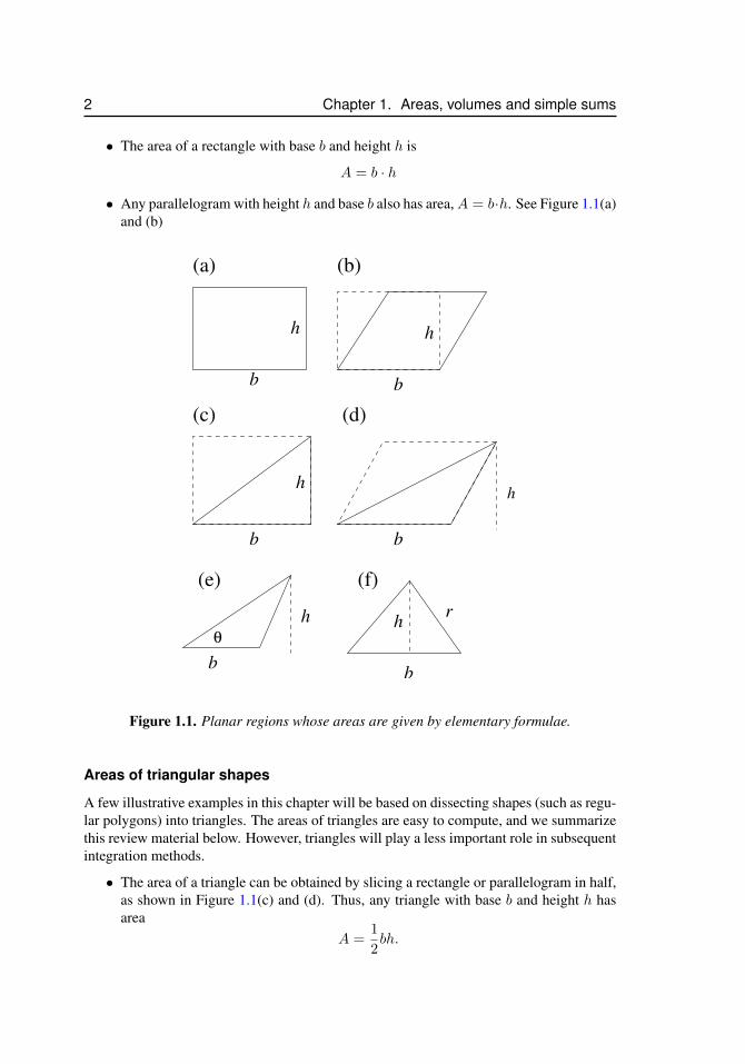
• The area of a rectangle with base b and height h is
A = b · h
• Any parallelogram with height h and base b also has area,A = b·h. See Figure 1.1(a)and (b)
(a)
(c)
(e) (f)
(d)
(b)
b
h
b
h
h
b
b
h r
b
h
b
θ
h
Figure 1.1. Planar regions whose areas are given by elementary formulae.
Areas of triangular shapes
A few illustrative examples in this chapter will be based on dissecting shapes (such as regu-lar polygons) into triangles. The areas of triangles are easy to compute, and we summarizethis review material below. However, triangles will play a less important role in subsequentintegration methods.
• The area of a triangle can be obtained by slicing a rectangle or parallelogram in half,as shown in Figure 1.1(c) and (d). Thus, any triangle with base b and height h hasarea
A =1
2bh.

1.2. Areas of simple shapes 3
• In some cases, the height of a triangle is not given, but can be determined from otherinformation provided. For example, if the triangle has sides of length b and r withenclosed angle θ, as shown on Figure 1.1(e) then its height is simply h = r sin(θ),and its area is
A = (1/2)br sin(θ)
• If the triangle is isosceles, with two sides of equal length, r, and base of length b,as in Figure 1.1(f) then its height can be obtained from Pythagoras’s theorem, i.e.h2 = r2 − (b/2)2 so that the area of the triangle is
A = (1/2)b√r2 − (b/2)2.
1.2.1 Example 1: Finding the area of a polygon usingtriangles: a “dissection” method
Using the simple ideas reviewed so far, we can determine the areas of more complex ge-ometric shapes. For example, let us compute the area of a regular polygon with n equalsides, where the length of each side is b = 1. This example illustrates how a complex shape(the polygon) can be dissected into simpler shapes, namely triangles1.
hθ1
1/2
θ/2
Figure 1.2. An equilateral n-sided polygon with sides of unit length can be dis-sected into n triangles. One of these triangles is shown at right. Since it can be furtherdivided into two Pythagorean triangles, trigonometric relations can be used to find theheight h in terms of the length of the base 1/2 and the angle θ/2.
Solution
The polygon has n sides, each of length b = 1. We dissect the polygon into n isoscelestriangles, as shown in Figure 1.2. We do not know the heights of these triangles, but theangle θ can be found. It is
θ = 2π/n
since together, n of these identical angles make up a total of 360◦ or 2π radians.1This calculation will be used again to find the area of a circle in Section 1.2.2. However, note that in later
chapters, our dissections of planar areas will focus mainly on rectangular pieces.

4 Chapter 1. Areas, volumes and simple sums
Let h stand for the height of one of the triangles in the dissected polygon. Thentrigonometric relations relate the height to the base length as follows:
oppadj
=b/2
h= tan(θ/2)
Using the fact that θ = 2π/n, and rearranging the above expression, we get
h =b
2 tan(π/n)
Thus, the area of each of the n triangles is
A =1
2bh =
1
2b
(b
2 tan(π/n)
).
The statement of the problem specifies that b = 1, so
A =1
2
(1
2 tan(π/n)
).
The area of the entire polygon is then n times this, namely
An-gon =n
4 tan(π/n).
For example, the area of a square (a polygon with 4 equal sides, n = 4) is
Asquare =4
4 tan(π/4)=
1
tan(π/4)= 1,
where we have used the fact that tan(π/4) = 1.As a second example, the area of a hexagon (6 sided polygon, i.e. n = 6) is
Ahexagon =6
4 tan(π/6)=
3
2(1/√
3)=
3√
3
2.
Here we used the fact that tan(π/6) = 1/√
3.
1.2.2 Example 2: How Archimedes discovered the area of acircle: dissect and “take a limit”
As we learn early in school the formula for the area of a circle of radius r, A = πr2.But how did this convenient formula come about? and how could we relate it to what weknow about simpler shapes whose areas we have discussed so far. Here we discuss howthis formula for the area of a circle was determined long ago by Archimedes using a clever“dissection” and approximation trick. We have already seen part of this idea in dissectinga polygon into triangles, in Section 1.2.1. Here we see a terrifically important second stepthat formed the “leap of faith” on which most of calculus is based, namely taking a limit asthe number of subdivisions increases 2.
First, we recall the definition of the constant π:2This idea has important parallels with our later development of integration. Here it involves adding up the
areas of triangles, and then taking a limit as the number of triangles gets larger. Later on, we do much the same,but using rectangles in the dissections.
1.2. Areas of simple shapes 5
Definition of π
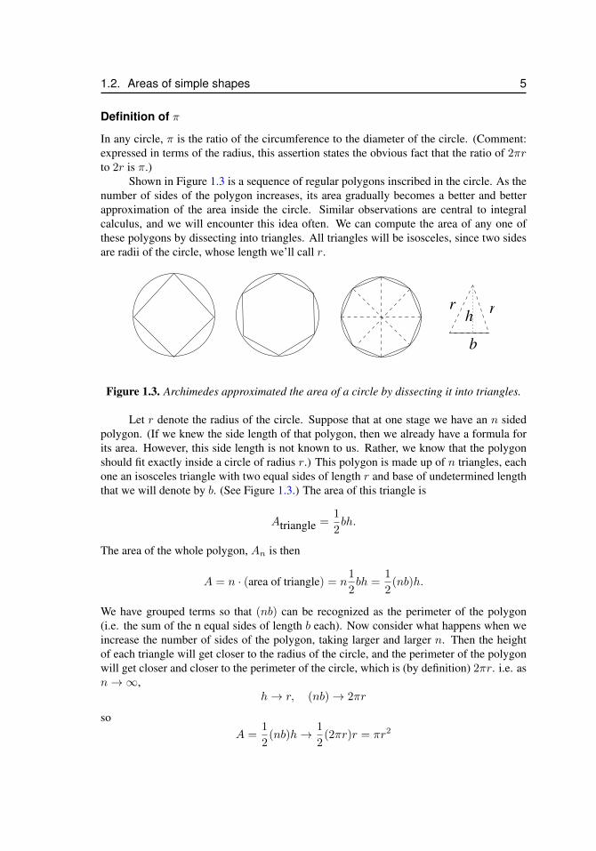
In any circle, π is the ratio of the circumference to the diameter of the circle. (Comment:expressed in terms of the radius, this assertion states the obvious fact that the ratio of 2πrto 2r is π.)
Shown in Figure 1.3 is a sequence of regular polygons inscribed in the circle. As thenumber of sides of the polygon increases, its area gradually becomes a better and betterapproximation of the area inside the circle. Similar observations are central to integralcalculus, and we will encounter this idea often. We can compute the area of any one ofthese polygons by dissecting into triangles. All triangles will be isosceles, since two sidesare radii of the circle, whose length we’ll call r.
r r
b
h
Figure 1.3. Archimedes approximated the area of a circle by dissecting it into triangles.
Let r denote the radius of the circle. Suppose that at one stage we have an n sidedpolygon. (If we knew the side length of that polygon, then we already have a formula forits area. However, this side length is not known to us. Rather, we know that the polygonshould fit exactly inside a circle of radius r.) This polygon is made up of n triangles, eachone an isosceles triangle with two equal sides of length r and base of undetermined lengththat we will denote by b. (See Figure 1.3.) The area of this triangle is
Atriangle =1
2bh.
The area of the whole polygon, An is then
A = n · (area of triangle) = n1
2bh =
1
2(nb)h.
We have grouped terms so that (nb) can be recognized as the perimeter of the polygon(i.e. the sum of the n equal sides of length b each). Now consider what happens when weincrease the number of sides of the polygon, taking larger and larger n. Then the heightof each triangle will get closer to the radius of the circle, and the perimeter of the polygonwill get closer and closer to the perimeter of the circle, which is (by definition) 2πr. i.e. asn→∞,
h→ r, (nb)→ 2πr
soA =
1
2(nb)h→ 1
2(2πr)r = πr2
6 Chapter 1. Areas, volumes and simple sums
We have used the notation “→” to mean that in the limit, as n gets large, the quantity ofinterest “approaches” the value shown. This argument proves that the area of a circle mustbe
A = πr2.
One of the most important ideas contained in this little argument is that by approximating ashape by a larger and larger number of simple pieces (in this case, a large number of trian-gles), we get a better and better approximation of its area. This idea will appear again soon,but in most of our standard calculus computations, we will use a collection of rectangles,rather than triangles, to approximate areas of interesting regions in the plane.
Areas of other shapes
We concentrate here the area of a circle and of other shapes.
• The area of a circle of radius r is
A = πr2.
• The surface area of a sphere of radius r is
Sball = 4πr2.
• The surface area of a right circular cylinder of height h and base radius r is
Scyl = 2πrh.
Units
The units of area can be meters2 (m2), centimeters2 (cm2), square inches, etc.
1.3 Simple volumesLater in this course, we will also be computing the volumes of 3D shapes. As in the caseof areas, we collect below some basic formulae for volumes of elementary shapes. Thesewill be useful in our later discussions.
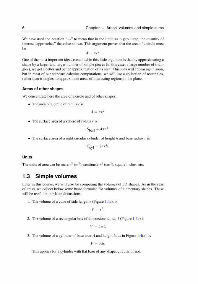
1. The volume of a cube of side length s (Figure 1.4a), is
V = s3.
2. The volume of a rectangular box of dimensions h, w, l (Figure 1.4b) is
V = hwl.
3. The volume of a cylinder of base area A and height h, as in Figure 1.4(c), is
V = Ah.
This applies for a cylinder with flat base of any shape, circular or not.
1.3. Simple volumes 7
r
(a) (b)
(c) (d)
s
w
l
h
A
h
Figure 1.4. 3-dimensional shapes whose volumes are given by elementary formulae
4. In particular, the volume of a cylinder with a circular base of radius r, (e.g. a disk) is
V = h(πr2).
5. The volume of a sphere of radius r (Figure 1.4d), is
V =4
3πr3.
6. The volume of a spherical shell (hollow sphere with a shell of some small thickness,τ ) is approximately
V ≈ τ · (surface area of sphere) = 4πτr2.
7. Similarly, a cylindrical shell of radius r, height h and small thickness, τ has volumegiven approximately by
V ≈ τ · (surface area of cylinder) = 2πτrh.
Units
The units of volume are meters3 (m3), centimeters3 (cm3), cubic inches, etc.
8 Chapter 1. Areas, volumes and simple sums
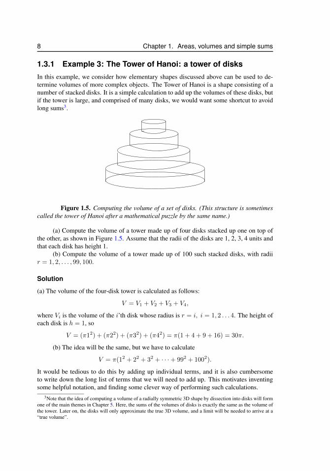
1.3.1 Example 3: The Tower of Hanoi: a tower of disksIn this example, we consider how elementary shapes discussed above can be used to de-termine volumes of more complex objects. The Tower of Hanoi is a shape consisting of anumber of stacked disks. It is a simple calculation to add up the volumes of these disks, butif the tower is large, and comprised of many disks, we would want some shortcut to avoidlong sums3.
Figure 1.5. Computing the volume of a set of disks. (This structure is sometimescalled the tower of Hanoi after a mathematical puzzle by the same name.)
(a) Compute the volume of a tower made up of four disks stacked up one on top ofthe other, as shown in Figure 1.5. Assume that the radii of the disks are 1, 2, 3, 4 units andthat each disk has height 1.
(b) Compute the volume of a tower made up of 100 such stacked disks, with radiir = 1, 2, . . . , 99, 100.
Solution
(a) The volume of the four-disk tower is calculated as follows:
V = V1 + V2 + V3 + V4,
where Vi is the volume of the i’th disk whose radius is r = i, i = 1, 2 . . . 4. The height ofeach disk is h = 1, so
V = (π12) + (π22) + (π32) + (π42) = π(1 + 4 + 9 + 16) = 30π.
(b) The idea will be the same, but we have to calculate
V = π(12 + 22 + 32 + · · ·+ 992 + 1002).
It would be tedious to do this by adding up individual terms, and it is also cumbersometo write down the long list of terms that we will need to add up. This motivates inventingsome helpful notation, and finding some clever way of performing such calculations.
3Note that the idea of computing a volume of a radially symmetric 3D shape by dissection into disks will formone of the main themes in Chapter 5. Here, the sums of the volumes of disks is exactly the same as the volume ofthe tower. Later on, the disks will only approximate the true 3D volume, and a limit will be needed to arrive at a“true volume”.
1.4. Sigma Notation 9
1.4 Sigma NotationLet’s consider the sequence of squared integers
(12, 22, 32, 42, 52, . . .) = (1, 4, 9, 16, 25, . . .)
and let’s add them up. Okay so the sum of the first square is 12 = 1, the sum of the firsttwo squares is 12 + 22 = 5, the sum of the first three squares is 12 + 22 + 32 = 14, etc.Now suppose we want to sum the first fifteen square integers–how should we write out thissum in our notes? Of course, the sum just looks like
12 + 22 + 32 + 42 + 52 + 62 + 72 + 82 + 92 + 102 + 112 + 122 + 132 + 142 + 152
which equals
1 + 4 + 9 + 16 + 25 + 36 + 49 + 64 + 81 + 100 + 121 + 144 + 169 + 196 + 225.
But let’s agree that the above expression is an eyesore. Frankly it occupies morespace than it deserves, is confusing to look at, and is logically redundant. All we wanted todo was ‘sum the first fifteen squared integers’, not ‘sum all the phone numbers that occurin the first fifteen pages of the phone book’. A sum with such a simple internal structureshould have a simple notation. Mathematicians and physicists have such a notation whichis convenient, logical, and simplifies many summations–this is the ‘sigma notation’.
The sum of the elements ak + ak+1 + · · ·+ an will be written∑nj=k aj , i.e.
n∑j=k
aj := ak + ak+1 + · · ·+ an.
The symbol Σ is the Greek letter for ‘S’ – we think of ‘S’ as standing for summation. Theexpression
∑nj=k aj represents the sum of the elements ak, ak+1, . . . , an. The letter ‘j’ is
the index of summation and is a dummy-variable, i.e. you are free to replace it by any letteror symbol you want (like k, `,m, n,♥, ?, . . .). Both
∑2013♣=1 a♣ and
∑20134=1 a4 stand for the
same sum: a1 + a2 + · · ·+ a2013. The notation j = k that appears underneath Σ indicateswhere the sum begins (i.e. which term starts off the series), and the superscript n tells uswhere it ends. We will be interested in getting used to this notation, as well as in actuallycomputing the value of the desired sum using a variety of shortcuts.
Simple examples
1. The convenience of the sigma notation is that the above sum of the first fifteensquared integers has now the more compact form
15∑j=1
j2.
We shall find below a closed-formula for this sum which will be easier to deriveusing the sigma notation.
10 Chapter 1. Areas, volumes and simple sums
2. Suppose we want to form the sum of ten numbers, each equal to 1. We would writethis as
S = 1 + 1 + 1 + . . . 1 ≡10∑k=1
1.
The notation . . . signifies that we have left out some of the terms (out of laziness,or in cases where there are too many to conveniently write down.) We could havejust as well written the sum with another symbol (e.g. n) as the index, i.e. the sameoperation is implied by
10∑n=1
1.
To compute the value of the sum we use the elementary fact that the sum of ten onesis just 10, so
S =
10∑k=1
1 = 10.
3. Sum of squares: Expand and sum the following:
S =
4∑k=1
k2.
Solution:
S =
4∑k=1
k2 = 1 + 22 + 32 + 42 = 1 + 4 + 9 + 16 = 30.
(We have already seen this sum in part (a) of The Tower of Hanoi.)
4. Common factors: Add up the following list of 100 numbers (only a few of them areshown):
S = 3 + 3 + 3 + 3 + · · ·+ 3.
Solution: There are 100 terms, all equal, so we can take out a common factor
S = 3 + 3 + 3 + 3 + · · ·+ 3 =
100∑k=1
3 = 3
100∑k=1
1 = 3(100) = 300.
5. Find the pattern: Write the following terms in summation notation:
S =1
3+
1
9+
1
27+
1
81.
Solution: We recognize that there is a pattern in the sequence of terms, namely, eachone is 1/3 raised to an increasing integer power, i.e.
S =1
3+
(1
3
)2
+
(1
3
)3
+
(1
3
)4
.
1.4. Sigma Notation 11
We can represent this with the “Sigma” notation as follows:
S =
4∑n=1
(1
3
)n.
The “index” n starts at 1, and counts up through 2, 3, and 4, while each term has theform of (1/3)n. This series is a geometric series, to be explored shortly. In mostcases, a standard geometric series starts off with the value 1. We can easily modifyour notation to include additional terms, for example:
S =
5∑n=0
(1
3
)n= 1 +
1
3+
(1
3
)2
+
(1
3
)3
+
(1
3
)4
+
(1
3
)5
.
Learning how to compute the sum of such terms will be important to us, and will bedescribed later on in this chapter.
6. Often there are different but equivalent ways to represent the same sum:
4 + 5 + 6 + 7 + 8 =
8∑j=4
j =
5∑j=1
(3 + j).
7. It is useful to have some dexterity in arranging and rearranging the Sigma notations.For instance, the sum
1− 2 + 3− 4 + 5− 6 + · · ·
has no upper bound and we may write
1− 2 + 3− 4 + 5− 6 + · · · =∞∑j=1
(−1)j+1j =
∞∑j=0
(−1)j(j + 1)
to highlight the fact that this sum has infinitely many terms.
8.
7 + 9 + 11 + 13 + 15 =
4∑j=0
(7 + 2j).
9.n∑j=n
aj = an.
10.1∑
j=10
aj = 0.
12 Chapter 1. Areas, volumes and simple sums
Manipulations of sums
Since addition is commutative and distributive, sums of lists of numbers satisfy many con-venient properties. We give a few examples below:
• Simplify the following expression:
10∑k=1
2k −10∑k=3
2k.
Solution: We have
10∑k=1
2k −10∑k=3
2k = (2 + 22 + 23 + · · ·+ 210)− (23 + · · ·+ 210) = 2 + 22.
Alternatively we could have arrived at this conclusion directly from
10∑k=1
2k −10∑k=3
2k =
2∑k=1
2k = 2 + 22 = 2 + 4 = 6.
The idea is that all but the first two terms in the first sum will cancel. The onlyremaining terms are those corresponding to k = 1 and k = 2.
• Expand the following expression:
5∑n=0
(1 + 3n).
Solution: We have5∑
n=0
(1 + 3n) =
5∑n=0
1 +
5∑n=0
3n.
1.4.1 Formulae for sums of integers, squares, and cubesThe general formulae are:
N∑k=1
k =N(N + 1)
2, (1.1)
N∑k=1
k2 =N(N + 1)(2N + 1)
6(1.2)
N∑k=1
k3 =
(N(N + 1)
2
)2
. (1.3)
We now provide a justification as to why these formulae are valid. The sum of the first Nintegers can perhaps most easily be seen by the following amusing argument.
1.4. Sigma Notation 13
The sum of consecutive integers (Gauss’ formula)
We first show that the sum SN of the first N integers is
SN = 1 + 2 + 3 + · · ·+N =
N∑k=1
k =N(N + 1)
2. (1.4)
The following trick is due to Gauss. By aligning two copies of the above sum, onewritten backwards, we can easily add them up one by one vertically. We see that:
SN = 1 + 2 + . . . + (N − 1) + N+
SN = N + (N − 1) + . . . + 2 + 1
2SN = (1 +N) + (1 +N) + . . . + (1 +N) + (1 +N)
Thus, there are N times the value (N + 1) above, so that
2SN = N(1 +N), so SN =N(1 +N)
2.
Thus, the formula is confirmed.
Example: Adding up the first 1000 integers
Suppose we want to add up the first 1000 integers. This formula is very useful in whatwould otherwise be a huge calculation. We find that
S = 1 + 2 + 3 + · · ·+ 1000 =
1000∑k=1
k =1000(1 + 1000)
2= 500(1001) = 500500.
Sums of squares and cubes
We now present an argument4verifying the above formulae for sums of squares and cubes.First, note that
(k + 1)3 − (k − 1)3 = 6k2 + 2,
son∑k=1
((k + 1)3 − (k − 1)3
)=
n∑k=1
(6k2 + 2).
But looking more carefully at the left hand side (LHS), we see that
n∑k=1
((k+ 1)3− (k−1)3) = 23−03 + 33−13 + 43−23 + 53−33...+ (n+ 1)3− (n−1)3
4contributed to these notes by Robert Israel.
14 Chapter 1. Areas, volumes and simple sums
so most of the terms cancel, leaving only −1 + n3 + (n+ 1)3. This means that
−1 + n3 + (n+ 1)3 = 6
n∑k=1
k2 +
n∑k=1
2,
son∑k=1
k2 =−1 + n3 + (n+ 1)3 − 2n
6=
2n3 + 3n2 + n
6.
Similarly, the formulae for∑nk=1 k and
∑nk=1 k
3, can be obtained by starting with theidentities
(k + 1)2 − (k − 1)2 = 4k, and (k + 1)4 − (k − 1)4 = 8k3 + 8k,
respectively. We encourage the interested reader to carry out these details.An alternative approach using a technique called mathematical induction to verify
the formulae for the sum of squares and cubes of integers is presented at the end of thischapter.
Example: Volume of a Tower of Hanoi, revisited
Armed with the formula for the sum of squares, we can now return to the problem of com-puting the volume of a tower of 100 stacked disks of heights 1 and radii r = 1, 2, . . . , 99, 100.We have
V = π(12+22+32+· · ·+992+1002) = π
100∑k=1
k2 = π100(101)(201)
6= 338, 350π cubic units.
Example
Compute the following sum:
Sa =
20∑k=1
(2− 3k + 2k2).
Solution
We can separate this into three individual sums, each of which can be handled by algebraicsimplification and/or use of the summation formulae developed so far.
Sa =
20∑k=1
(2− 3k + 2k2) = 2
20∑k=1
1− 3
20∑k=1
k + 2
20∑k=1
k2.
Thus, we get
Sa = 2(20)− 3
(20(21)
2
)+ 2
((20)(21)(41)
6
)= 5150.
1.5. Summing the geometric series 15
Example
Compute the following sum:
Sb =
50∑k=10
k.
Solution
We can express the second sum as a difference of two sums:
Sb =
50∑k=10
k =
(50∑k=1
k
)−
(9∑k=1
k
).
Thus
Sb =
(50(51)
2− 9(10)
2
)= 1275− 45 = 1230.
1.5 Summing the geometric seriesConsider a sum of terms that all have the form rk, where r is some real number and k isan integer power. We refer to a series of this type as a geometric series. We have alreadyseen one example of this type in a previous section. Below we will show that the sum ofsuch a series is given by:
SN = 1 + r + r2 + r3 + . . .+ rN =
N∑k=0
rk =1− rN+1
1− r(1.5)
where r 6= 1. We call this sum a (finite) geometric series. We would like to findan expression for terms of this form in the general case of any real number r, and finitenumber of terms N . First we note that there are N + 1 terms in this sum, so that if r = 1then
SN = 1 + 1 + 1 + . . . 1 = N + 1
(a total of N + 1 ones added.) If r 6= 1 we have the following trick:
SN = 1 + r + r2 + . . . + rN
−r SN = r + r2 + . . . + rN+1
Subtracting leads to
SN − r SN = (1 + r + r2 + · · ·+ rN )− (r + r2 + · · ·+ rN + rN+1)
Most of the terms on the right hand side cancel, leaving
SN (1− r) = 1− rN+1.
16 Chapter 1. Areas, volumes and simple sums
Now dividing both sides by 1− r leads to
SN =1− rN+1
1− r,
which was the formula to be established.
Example: Geometric series
Compute the following sum:
Sc =
10∑k=0
2k.
Solution
This is a geometric series
Sc =
10∑k=0
2k =1− 210+1
1− 2=
1− 2048
−1= 2047.
1.6 Prelude to infinite seriesSo far, we have looked at several examples of finite series, i.e. series in which there areonly a finite number of terms, N (where N is some integer). We would like to investigatehow the sum of a series behaves when more and more terms of the series are included. Itis evident that in many cases, such as Gauss’s series (1.4), or sums of squared or cubedintegers (e.g., Eqs. (1.2) and (1.3)), the series simply gets larger and larger as more termsare included. We say that such series diverge as N → ∞. Here we will look specificallyfor series that converge, i.e. have a finite sum, even as more and more terms are included5.
Let us focus again on the geometric series and determine its behaviour when thenumber of terms is increased. Our goal is to find a way of attaching a meaning to theexpression
S =
∞∑k=0
rk,
when the series becomes an infinite series. We will use the following definition:
1.6.1 The infinite geometric seriesDefinition
An infinite series that has a unique, finite sum is said to be convergent. Otherwise it isdivergent.
5Convergence and divergence of series is discussed in fuller depth in Chapter 11. However, these concepts areso important that some preliminary ideas need to be introduced early in the term.
1.6. Prelude to infinite series 17
Definition
Suppose that S is an (infinite) series whose terms are ak. Then the partial sums, Sn, of thisseries are
Sn =
n∑k=0
ak.
We say that the sum of the infinite series is S, and write
S =
∞∑k=0
ak,
provided that
S = limn→∞
n∑k=0
ak.
That is, we consider the infinite series as the limit of the partial sums as the number ofterms n is increased. In this case we also say that the infinite series converges to S.
We will see that only under certain circumstances will infinite series have a finitesum, and we will be interested in exploring two questions:
1. Under what circumstances does an infinite series have a finite sum.
2. What value does the partial sum approach as more and more terms are included.
In the case of a geometric series, the sum of the series, (1.5) depends on the number ofterms in the series, n via rn+1. Whenever r > 1, or r < −1, this term will get bigger inmagnitude as n increases, whereas, for 0 < r < 1, this term decreases in magnitude withn. We can say that
limn→∞
rn+1 = 0 provided |r| < 1.
These observations are illustrated by two specific examples below. This leads to the fol-lowing conclusion:
The sum of an infinite geometric series,
S = 1 + r + r2 + · · ·+ rk + · · · =∞∑k=0
rk,
exists provided |r| < 1 and is
S =1
1− r. (1.6)
Examples of convergent and divergent geometric series are discussed below.
18 Chapter 1. Areas, volumes and simple sums
1.6.2 Example: A geometric series that converges.Consider the geometric series with r = 1
2 , i.e.
Sn = 1 +1
2+
(1
2
)2
+
(1
2
)3
+ . . .+
(1
2
)n=
n∑k=0
(1
2
)k.
Then
Sn =1− (1/2)n+1
1− (1/2).
We observe that as n increases, i.e. as we retain more and more terms, we obtain
limn→∞
Sn = limn→∞
1− (1/2)n+1
1− (1/2)=
1
1− (1/2)= 2.
In this case, we write∞∑n=0
(1
2
)n= 1 +
1
2+ (
1
2)2 + . . . = 2
and we say that “the (infinite) series converges to 2”.
1.6.3 Example: A geometric series that divergesIn contrast, we now investigate the case that r = 2: then the series consists of terms
Sn = 1 + 2 + 22 + 23 + . . .+ 2n =
n∑k=0
2k =1− 2n+1
1− 2= 2n+1 − 1
We observe that as n grows larger, the sum continues to grow indefinitely. In this case, wesay that the sum does not converge, or, equivalently, that the sum diverges.
It is important to remember that an infinite series, i.e. a sum with infinitely manyterms added up, can exhibit either one of these two very different behaviours. It mayconverge in some cases, as the first example shows, or diverge (fail to converge) in othercases. We will see examples of each of these trends again. It is essential to be able todistinguish the two. Divergent series (or series that diverge under certain conditions) mustbe handled with particular care, for otherwise, we may find contradictions or seeminglyreasonable calculations that have meaningless results.
1.7 Application of geometric series to the branchingstructure of the lungs
In this section, we will compute the volume and surface area of the branched airways oflungs6. We use the summation formulae to arrive at the results, and we also illustrate howthe same calculation could be handled using a simple spreadsheet.
6This section provides an example of how to set up a biologically relevant calculation based on geometricseries. It is further studied in the homework problems. A similar example is given as an exercise for the studentin Lab 1 of this calculus course.
1.7. Application of geometric series to the branching structure of the lungs 19
Our lungs pack an amazingly large surface area into a confined volume. Most ofthe oxygen exchange takes place in tiny sacs called alveoli at the terminal branches of theairways passages. The bronchial tubes conduct air, and distribute it to the many smallerand smaller tubes that eventually lead to those alveoli. The principle of this efficient organfor oxygen exchange is that these very many small structures present a very large surfacearea. Oxygen from the air can diffuse across this area into the bloodstream very efficiently.
The lungs, and many other biological “distribution systems” are composed of abranched structure. The initial segment is quite large. It bifurcates into smaller segments,which then bifurcate further, and so on, resulting in a geometric expansion in the number ofbranches, their collective volume, length, etc. In this section, we apply geometric series toexplore this branched structure of the lung. We will construct a simple mathematical modeland explore its consequences. The model will consist in some well-formulated assumptionsabout the way that “daughter branches” are related to their “parent branch”. Based on theseassumptions, and on tools developed in this chapter, we will then predict properties of thestructure as a whole. We will be particularly interested in the volume V and the surfacearea S of the airway passages in the lungs7.
2
l0
r0
Segment 0
1
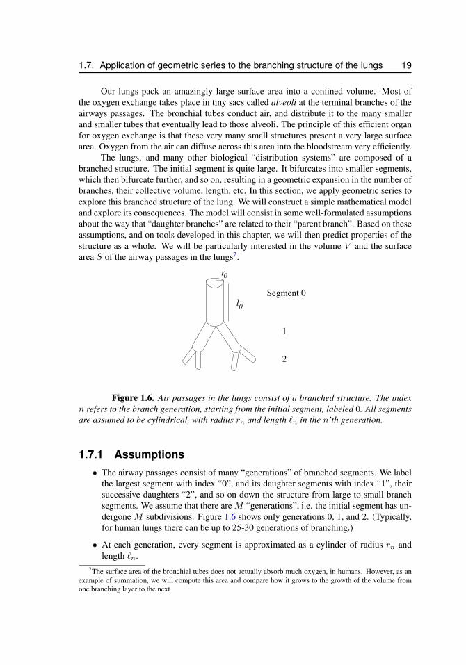
Figure 1.6. Air passages in the lungs consist of a branched structure. The indexn refers to the branch generation, starting from the initial segment, labeled 0. All segmentsare assumed to be cylindrical, with radius rn and length `n in the n’th generation.
1.7.1 Assumptions• The airway passages consist of many “generations” of branched segments. We label
the largest segment with index “0”, and its daughter segments with index “1”, theirsuccessive daughters “2”, and so on down the structure from large to small branchsegments. We assume that there are M “generations”, i.e. the initial segment has un-dergone M subdivisions. Figure 1.6 shows only generations 0, 1, and 2. (Typically,for human lungs there can be up to 25-30 generations of branching.)
• At each generation, every segment is approximated as a cylinder of radius rn andlength `n.
7The surface area of the bronchial tubes does not actually absorb much oxygen, in humans. However, as anexample of summation, we will compute this area and compare how it grows to the growth of the volume fromone branching layer to the next.

20 Chapter 1. Areas, volumes and simple sums
radius of first segment r0 0.5 cmlength of first segment `0 5.6 cmratio of daughter to parent length α 0.9ratio of daughter to parent radius β 0.86number of branch generations M 30average number daughters per parent b 1.7
Table 1.1. Typical structure of branched airway passages in lungs.
• The number of branches grows along the “tree”. On average, each parent branchproduces b daughter branches. In Figure 1.6, we have illustrated this idea for b = 2.A branched structure in which each branch produces two daughter branches is de-scribed as a bifurcating tree structure (whereas trifurcating implies b = 3). In reallungs, the branching is slightly irregular. Not every level of the structure bifurcates,but in general, averaging over the many branches in the structure b is smaller than 2.In fact, the rule that links the number of branches in generation n, here denoted xnwith the number (of smaller branches) in the next generation, xn+1 is
xn+1 = bxn. (1.7)
We will assume, for simplicity, that b is a constant. Since the number of branchesis growing down the length of the structure, it must be true that b > 1. For humanlungs, on average, 1 < b < 2. Here we will take b to be constant, i.e. b = 1.7. Inactual fact, this simplification cannot be precise, because we have just one segmentinitially (x0 = 1), and at level 1, the number of branches x1 should be some smallinteger, not a number like “1.7”. However, as in many mathematical models, someaccuracy is sacrificed to get intuition. Later on, details that were missed and areconsidered important can be corrected and refined.
• The ratios of radii and lengths of daughters to parents are approximated by “pro-portional scaling”. This means that the relationship of the radii and lengths satisfysimple rules: The lengths are related by
`n+1 = α`n, (1.8)
and the radii are related byrn+1 = βrn, (1.9)
with α and β positive constants. For example, it could be the case that the radius ofdaughter branches is 1/2 or 2/3 that of the parent branch. Since the branches decreasein size (while their number grows), we expect that 0 < α < 1 and 0 < β < 1.
Rules such as those given by equations (1.8) and (1.9) are often called self-similar growthlaws. Such concepts are closely linked to the idea of fractals, i.e. theoretical structuresproduced by iterating such growth laws indefinitely. In a real biological structure, the
1.7. Application of geometric series to the branching structure of the lungs 21
number of generations is finite. (However, in some cases, a finite geometric series is well-approximated by an infinite sum.)
Actual lungs are not fully symmetric branching structures, but the above approxi-mations are used here for simplicity. According to physiological measurements, the scalefactors for sizes of daughter to parent size are in the range 0.65 ≤ α, β ≤ 0.9. (K. G.Horsfield, G. Dart, D. E. Olson, and G. Cumming, (1971) J. Appl. Phys. 31, 207-217.) Forthe purposes of this example, we will use the values of constants given in Table 1.1.
1.7.2 A simple geometric ruleThe three equations that govern the rules for successive branching, i.e. equations (1.7), (1.8),and (1.9), are examples of a very generic “geometric progression” recipe. Before returningto the problem at hand, let us examine the implications of this recursive rule, when it isapplied to generating the whole structure. Essentially, we will see that the rule linking twogenerations implies an exponential growth. To see this, let us write out a few first terms inthe progression of the sequence {xn}:
initial value: x0
first iteration: x1= bx0
second iteration: x2= bx1 = b(bx0) = b2x0
third iteration: x3= bx2 = b(b2x0) = b3x0
...
By the same pattern, at the n’th generation, the number of segments will be
n’th iteration: xn = bxn−1 = b(bxn−2) = b(b(bxn−3)) = · · · = (b · b · · · b)︸ ︷︷ ︸n factors
x0 = bnx0.
We have arrived at a simple, but important result, namely:
The rule linking two generations,xn = bxn−1 (1.10)
implies that the n’th generation will have grown by a factor bn, i.e.,
xn = bnx0. (1.11)
This connection between the rule linking two generations and the resulting number ofmembers at each generation is useful in other circumstances. Equation (1.10) is sometimescalled a recursion relation, and its solution is given by equation (1.11). We will use thesame idea to find the connection between the volumes, and surface areas of successivesegments in the branching structure.
22 Chapter 1. Areas, volumes and simple sums
1.7.3 Total number of segmentsWe used the result of Section 1.7.2 and the fact that there is one segment in the 0’th gener-ation, i.e. x0 = 1, to conclude that at the n’th generation, the number of segments is
xn = x0bn = 1 · bn = bn.
For example, if b = 2, the number of segments grows by powers of 2, so that the treebifurcates with the pattern 1, 2, 4, 8, etc.
To determine how many branch segments there are in total, we add up over all gen-erations, 0, 1, . . .M . This is a geometric series, whose sum we can compute. Using equa-tion (1.5), we find
N =
M∑n=0
bn =
(1− bM+1
1− b
).
Given b and M , we can then predict the exact number of segments in the structure. Thecalculation is summarized further on for values of the branching parameter, b, and thenumber of branch generations, M , given in Table 1.1.
1.7.4 Total volume of airways in the lungSince each lung segment is assumed to be cylindrical, its volume is
vn = πr2n`n.
Here we mean just a single segment in the n’th generation of branches. (There are bn suchidentical segments in the n’th generation, and we will refer to the volume of all of themtogether as Vn below.)
The length and radius of segments also follow a geometric progression. In fact, thesame idea developed above can be used to relate the length and radius of a segment in then’th, generation segment to the length and radius of the original 0’th generation segment,namely,
`n = α`n−1 ⇒ `n = αn`0,
andrn = βrn−1 ⇒ rn = βnr0.
Thus the volume of one segment in generation n is
vn = πr2n`n = π(βnr0)2(αn`0) = (αβ2)n (πr2
0`0)︸ ︷︷ ︸v0
.
This is just a product of the initial segment volume v0 = πr20`0, with the n’th power of a
certain factor(α, β). (That factor takes into account that both the radius and the length arebeing scaled down at every successive generation of branching.) Thus
vn = (αβ2)nv0.
1.7. Application of geometric series to the branching structure of the lungs 23
The total volume of all (bn) segments in the n’th layer is
Vn = bnvn = bn(αβ2)nv0 = (bαβ2︸ ︷︷ ︸a
)n v0.
Here we have grouped terms together to reveal the simple structure of the relationship:one part of the expression is just the initial segment volume, while the other is now a“scale factor” that includes not only changes in length and radius, but also in the number ofbranches. Letting the constant a stand for that scale factor, a = (bαβ2) leads to the resultthat the volume of all segments in the n’th layer is
Vn = anv0.
The total volume of the structure is obtained by summing the volumes obtained ateach layer. Since this is a geometric series, we can use the summation formula. i.e.,Equation (1.5). Accordingly, total airways volume is
V =
30∑n=0
Vn = v0
30∑n=0
an = v0
(1− aM+1
1− a
).
The similarity of treatment with the previous calculation of number of branches is appar-ent. We compute the value of the constant a in Table 1.2, and find the total volume inSection 1.7.6.
1.7.5 Total surface area of the lung branchesThe surface area of a single segment at generation n, based on its cylindrical shape, is
sn = 2πrn`n = 2π(βnr0)(αn`0) = (αβ)n (2πr0`0)︸ ︷︷ ︸s0
,
where s0 is the surface area of the initial segment. Since there are bn branches at generationn, the total surface area of all the n’th generation branches is thus
Sn = bn(αβ)ns0 = (bαβ︸︷︷︸c
)ns0,
where we have let c stand for the scale factor c = (bαβ). Thus,
Sn = cns0.
This reveals the similar nature of the problem. To find the total surface area of the airways,we sum up,
S = s0
M∑n=0
cn = s0
(1− cM+1
1− c
).
We compute the values of s0 and c in Table 1.2, and summarize final calculations of thetotal airways surface area in section 1.7.6.
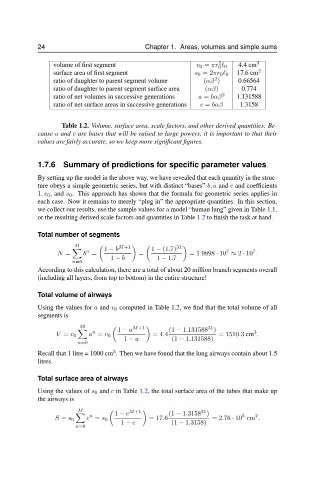
24 Chapter 1. Areas, volumes and simple sums
volume of first segment v0 = πr20`0 4.4 cm3
surface area of first segment s0 = 2πr0`0 17.6 cm2
ratio of daughter to parent segment volume (αβ2) 0.66564ratio of daughter to parent segment surface area (αβ) 0.774ratio of net volumes in successive generations a = bαβ2 1.131588ratio of net surface areas in successive generations c = bαβ 1.3158
Table 1.2. Volume, surface area, scale factors, and other derived quantities. Be-cause a and c are bases that will be raised to large powers, it is important to that theirvalues are fairly accurate, so we keep more significant figures.
1.7.6 Summary of predictions for specific parameter valuesBy setting up the model in the above way, we have revealed that each quantity in the struc-ture obeys a simple geometric series, but with distinct “bases” b, a and c and coefficients1, v0, and s0. This approach has shown that the formula for geometric series applies ineach case. Now it remains to merely “plug in” the appropriate quantities. In this section,we collect our results, use the sample values for a model “human lung” given in Table 1.1,or the resulting derived scale factors and quantities in Table 1.2 to finish the task at hand.
Total number of segments
N =
M∑n=0
bn =
(1− bM+1
1− b
)=
(1− (1.7)31
1− 1.7
)= 1.9898 · 107 ≈ 2 · 107.
According to this calculation, there are a total of about 20 million branch segments overall(including all layers, from top to bottom) in the entire structure!
Total volume of airways
Using the values for a and v0 computed in Table 1.2, we find that the total volume of allsegments is
V = v0
30∑n=0
an = v0
(1− aM+1
1− a
)= 4.4
(1− 1.13158831)
(1− 1.131588)= 1510.3 cm3.
Recall that 1 litre = 1000 cm3. Then we have found that the lung airways contain about 1.5litres.
Total surface area of airways
Using the values of s0 and c in Table 1.2, the total surface area of the tubes that make upthe airways is
S = s0
M∑n=0
cn = s0
(1− cM+1
1− c
)= 17.6
(1− 1.315831)
(1− 1.3158)= 2.76 · 105 cm2.
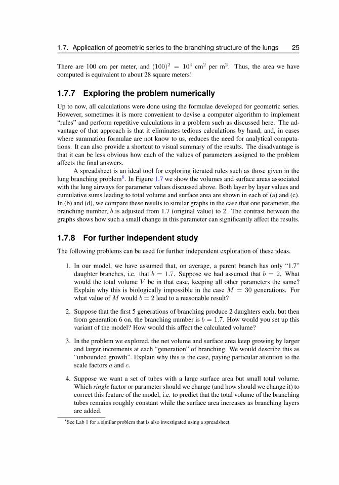
1.7. Application of geometric series to the branching structure of the lungs 25
There are 100 cm per meter, and (100)2 = 104 cm2 per m2. Thus, the area we havecomputed is equivalent to about 28 square meters!
1.7.7 Exploring the problem numericallyUp to now, all calculations were done using the formulae developed for geometric series.However, sometimes it is more convenient to devise a computer algorithm to implement“rules” and perform repetitive calculations in a problem such as discussed here. The ad-vantage of that approach is that it eliminates tedious calculations by hand, and, in caseswhere summation formulae are not know to us, reduces the need for analytical computa-tions. It can also provide a shortcut to visual summary of the results. The disadvantage isthat it can be less obvious how each of the values of parameters assigned to the problemaffects the final answers.
A spreadsheet is an ideal tool for exploring iterated rules such as those given in thelung branching problem8. In Figure 1.7 we show the volumes and surface areas associatedwith the lung airways for parameter values discussed above. Both layer by layer values andcumulative sums leading to total volume and surface area are shown in each of (a) and (c).In (b) and (d), we compare these results to similar graphs in the case that one parameter, thebranching number, b is adjusted from 1.7 (original value) to 2. The contrast between thegraphs shows how such a small change in this parameter can significantly affect the results.
1.7.8 For further independent studyThe following problems can be used for further independent exploration of these ideas.
1. In our model, we have assumed that, on average, a parent branch has only “1.7”daughter branches, i.e. that b = 1.7. Suppose we had assumed that b = 2. Whatwould the total volume V be in that case, keeping all other parameters the same?Explain why this is biologically impossible in the case M = 30 generations. Forwhat value of M would b = 2 lead to a reasonable result?
2. Suppose that the first 5 generations of branching produce 2 daughters each, but thenfrom generation 6 on, the branching number is b = 1.7. How would you set up thisvariant of the model? How would this affect the calculated volume?
3. In the problem we explored, the net volume and surface area keep growing by largerand larger increments at each “generation” of branching. We would describe this as“unbounded growth”. Explain why this is the case, paying particular attention to thescale factors a and c.
4. Suppose we want a set of tubes with a large surface area but small total volume.Which single factor or parameter should we change (and how should we change it) tocorrect this feature of the model, i.e. to predict that the total volume of the branchingtubes remains roughly constant while the surface area increases as branching layersare added.
8See Lab 1 for a similar problem that is also investigated using a spreadsheet.
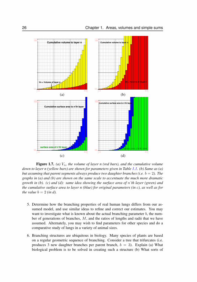
26 Chapter 1. Areas, volumes and simple sums
Cumulative volume to layer n
Vn = Volume of layer n
||V
-0.5 30.5
0.0
1500.0
Cumulative volume to layer n
Vn = Volume of layer n
-0.5 30.5
0.0
1500.0
(a) (b)
Cumulative surface area to n’th layer
surface area of n’th layer
-0.5 30.5
0.0
250000.0
Cumulative surface area to n’th layer
surface area of n’th layer
-0.5 30.5
0.0
250000.0
(c) (d)
Figure 1.7. (a) Vn, the volume of layer n (red bars), and the cumulative volumedown to layer n (yellow bars) are shown for parameters given in Table 1.1. (b) Same as (a)but assuming that parent segments always produce two daughter branches (i.e. b = 2). Thegraphs in (a) and (b) are shown on the same scale to accentuate the much more dramaticgrowth in (b). (c) and (d): same idea showing the surface area of n’th layer (green) andthe cumulative surface area to layer n (blue) for original parameters (in c), as well as forthe value b = 2 (in d).
5. Determine how the branching properties of real human lungs differs from our as-sumed model, and use similar ideas to refine and correct our estimates. You maywant to investigate what is known about the actual branching parameter b, the num-ber of generations of branches, M , and the ratios of lengths and radii that we haveassumed. Alternately, you may wish to find parameters for other species and do acomparative study of lungs in a variety of animal sizes.
6. Branching structures are ubiquitous in biology. Many species of plants are basedon a regular geometric sequence of branching. Consider a tree that trifurcates (i.e.produces 3 new daughter branches per parent branch, b = 3). Explain (a) Whatbiological problem is to be solved in creating such a structure (b) What sorts of
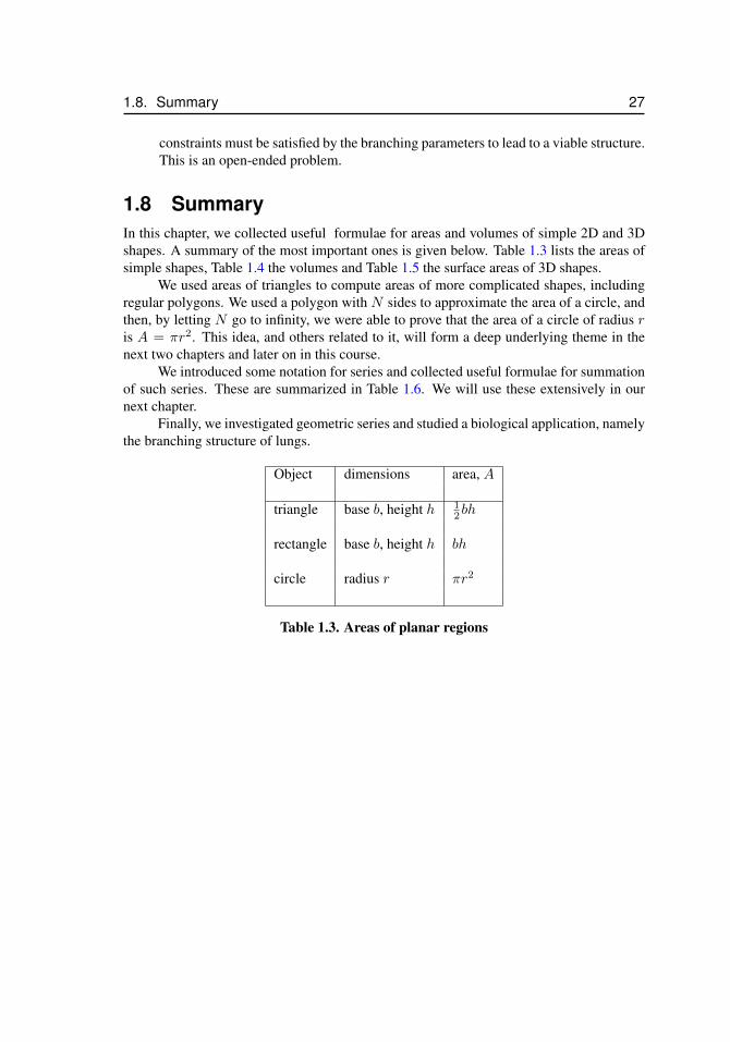
1.8. Summary 27
constraints must be satisfied by the branching parameters to lead to a viable structure.This is an open-ended problem.
1.8 SummaryIn this chapter, we collected useful formulae for areas and volumes of simple 2D and 3Dshapes. A summary of the most important ones is given below. Table 1.3 lists the areas ofsimple shapes, Table 1.4 the volumes and Table 1.5 the surface areas of 3D shapes.
We used areas of triangles to compute areas of more complicated shapes, includingregular polygons. We used a polygon with N sides to approximate the area of a circle, andthen, by letting N go to infinity, we were able to prove that the area of a circle of radius ris A = πr2. This idea, and others related to it, will form a deep underlying theme in thenext two chapters and later on in this course.
We introduced some notation for series and collected useful formulae for summationof such series. These are summarized in Table 1.6. We will use these extensively in ournext chapter.
Finally, we investigated geometric series and studied a biological application, namelythe branching structure of lungs.
Object dimensions area, A
triangle base b, height h 12bh
rectangle base b, height h bh
circle radius r πr2
Table 1.3. Areas of planar regions
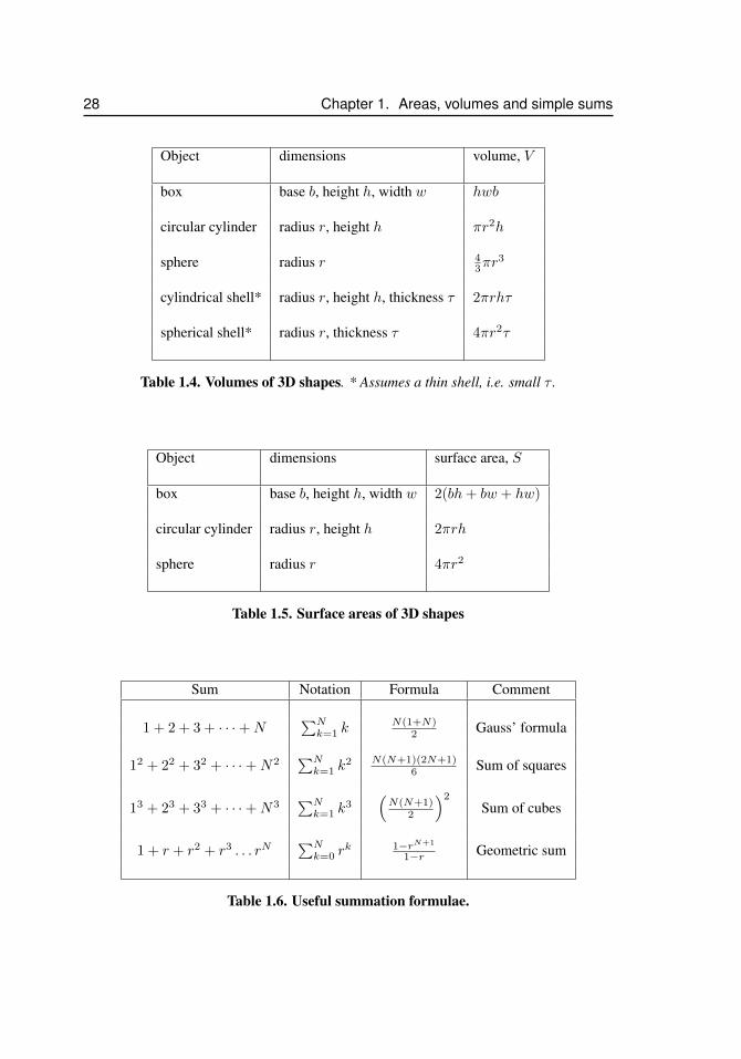
28 Chapter 1. Areas, volumes and simple sums
Object dimensions volume, V
box base b, height h, width w hwb
circular cylinder radius r, height h πr2h
sphere radius r 43πr
3
cylindrical shell* radius r, height h, thickness τ 2πrhτ
spherical shell* radius r, thickness τ 4πr2τ
Table 1.4. Volumes of 3D shapes. * Assumes a thin shell, i.e. small τ .
Object dimensions surface area, S
box base b, height h, width w 2(bh+ bw + hw)
circular cylinder radius r, height h 2πrh
sphere radius r 4πr2
Table 1.5. Surface areas of 3D shapes
Sum Notation Formula Comment
1 + 2 + 3 + · · ·+N∑Nk=1 k
N(1+N)2 Gauss’ formula
12 + 22 + 32 + · · ·+N2∑Nk=1 k
2 N(N+1)(2N+1)6 Sum of squares
13 + 23 + 33 + · · ·+N3∑Nk=1 k
3(N(N+1)
2
)2
Sum of cubes
1 + r + r2 + r3 . . . rN∑Nk=0 r
k 1−rN+1
1−r Geometric sum
Table 1.6. Useful summation formulae.
1.9. Optional Material 29
1.9 Optional Material1.9.1 How to prove the formulae for sums of squares and
cubesMathematicians are concerned with rigorously establishing formulae such as sums of squared(or cubed) integers. While it is not hard to see that these formulae “work” for a few cases,determining that they work in general requires more work. Here we provide a taste of howsuch careful arguments works. We give two examples. The first, based on mathematicalinduction provides a general method that could be used in many similar kinds of proofs.The second argument, also for purposes of illustration uses a “trick”. Devising such tricksis not as straightforward, and depends to some degree on serendipity or experience withnumbers.
Proof by induction
Here, we prove the formula for the sum of square integers,
N∑k=1
k2 =N(N + 1)(2N + 1)
6,
using a technique called induction. The idea of the method is to check that the formulaworks for one or two simple cases (e.g. the “sum” of just one or just two terms of theseries), and then show that whenever it works for one case (summing up to N ), it has toalso work for the next case (summing up to N + 1).
First, we verify that this formula works for a few test cases:N = 1: If there is only one term, then clearly, by inspection,
1∑k=1
k2 = 12 = 1.
The formula indicates that we should get
S =1(1 + 1)(2 · 1 + 1)
6=
1(2)(3)
6= 1,
so this case agrees with the prediction.N = 2:
2∑k=1
k2 = 12 + 22 = 1 + 4 = 5.
The formula would then predict that
S =2(2 + 1)(2 · 2 + 1)
6=
2(3)(5)
6= 5.
So far, elementary computation matches with the result predicted by the formula.Now we show that if this formula holds for any one case, e.g. for the sum of the first N
30 Chapter 1. Areas, volumes and simple sums
squares, then it is also true for the next case, i.e. for the sum of N + 1 squares. So we willassume that someone has checked that for some particular value of N it is true that
SN =
N∑k=1
k2 =N(N + 1)(2N + 1)
6.
Now the sum of the first N + 1 squares will be just a bit bigger: it will have one more termadded to it:
SN+1 =
N+1∑k=1
k2 =
N∑k=1
k2 + (N + 1)2.
Thus
SN+1 =N(N + 1)(2N + 1)
6+ (N + 1)2.
Combining terms, we get
SN+1 = (N + 1)
[N(2N + 1)
6+ (N + 1)
],
SN+1 = (N + 1)2N2 +N + 6N + 6
6= (N + 1)
2N2 + 7N + 6
6.
Simplifying and factoring the last term leads to
SN+1 = (N + 1)(2N + 3)(N + 2)
6.
We want to check that this still agrees with what the formula predicts. To make the notationsimpler, we will let M stand for N + 1. Then, expressing the result in terms of the quantityM = N + 1 we get
SM =
M∑k=1
k2 = (N + 1)[2(N + 1) + 1][(N + 1) + 1]
6= M
[2M + 1][M + 1]
6.
This is the same formula as we started with, only written in terms of M instead of N . Thuswe have verified that the formula works. By Mathematical Induction we find that the resulthas been proved.
1.10. Exercises 31
1.10 ExercisesExercise 1.1 Answer the following questions:
(a) What is the value of the fifth term of the sum S =20∑k=1
(5 + 3k)/k?
(b) How many terms are there in total in the sum S =17∑k=7
ek?
(c) Write out the terms in5∑
n=12n−1.
(d) Write out the terms in4∑
n=02n.
(e) Write the series 1 + 3 + 32 + 33 in summation notation in two equivalent forms.
Exercise 1.2 Summation notation
(a) Write 2 + 4 + 6 + 8 + 10 + 12 + ... in summation notation.
(b) Write 1 + 12 + 1
3 + 14 + ... in summation notation.
(c) Write out the first few terms of100∑i=0
3i
(d) Write out the first few terms of∞∑n=1
1
nn
(e) Simplify∞∑k=5
(1
2
)k+
4∑k=2
(1
2
)k
(f) Simplify50∑x=0
3x −50∑
x=10
3x
(g) Simplify100∑n=0
n+
100∑n=0
n2
(h) Simplify 2
100∑y=0
y +
100∑y=0
y2 +
100∑y=0
1
Exercise 1.3 Show that the following pairs of sums are equivalent:
(a)10∑m=0
(m+ 1)2 and11∑n=1
n2
32 Chapter 1. Areas, volumes and simple sums
(b)4∑
n=1
(n2 − 2n+ 1) and4∑
n=1
(n− 1)2
Exercise 1.4 Compute the following sums: (Some of the calculations will be facilitatedby a calculator)
(a)290∑i=1
1 (b)150∑i=1
2 (c)80∑i=1
3
(d)50∑n=1
n (e)60∑n=1
n (f)60∑
n=10
n
(g)100∑n=20
n (h)25∑n=1
3n2 (i)20∑n=1
2n2
(j)55∑i=1
(i+ 2) (k)75∑i=1
(i+ 1) (l)500∑k=100
k
(m)100∑k=50
k (n)50∑k=2
(k2 − 2k + 1) (o)50∑k=5
(k2 − 2k + 1)
(p)20∑
m=10
m3 (q)15∑m=0
(m+ 1)3
For the solutions to these, we will use several summation formulae, and the notation shownbelow for convenience:
S0(n) =
n∑i=1
1 = n S1(n) =
n∑i=1
i =n(n+ 1)
2
S2(n) =
n∑i=1
i2 =n(n+ 1)(2n+ 1)
6S3(n) =
n∑i=1
i3 =
[n(n+ 1)
2
]2
Exercise 1.5 Use the sigma summation notation to set up the following problems, andthen apply known formulae to compute the sums.
(a) Find the sum of the first 50 even numbers, 2 + 4 + 6 + ...
(b) Find the sum of the first 50 odd numbers, 1 + 3 + ...
(c) Find the sum of the first 50 integers of the form n(n+ 1) where n = 1, 2, .., 50.
(d) Consider all the integers that are of the form n(n− 1) where n = 1, 2, 3 . . .. Find thesum of the first 50 such numbers.
Exercise 1.6 Compute the following sum.
S =
12∑i=1
i(1− i) + 2i
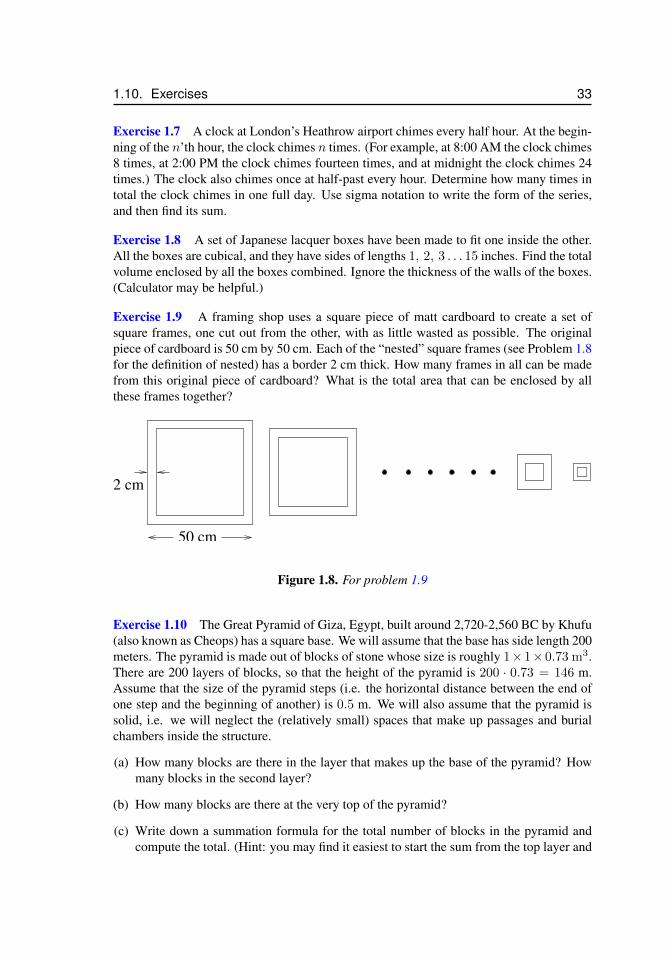
1.10. Exercises 33
Exercise 1.7 A clock at London’s Heathrow airport chimes every half hour. At the begin-ning of the n’th hour, the clock chimes n times. (For example, at 8:00 AM the clock chimes8 times, at 2:00 PM the clock chimes fourteen times, and at midnight the clock chimes 24times.) The clock also chimes once at half-past every hour. Determine how many times intotal the clock chimes in one full day. Use sigma notation to write the form of the series,and then find its sum.
Exercise 1.8 A set of Japanese lacquer boxes have been made to fit one inside the other.All the boxes are cubical, and they have sides of lengths 1, 2, 3 . . . 15 inches. Find the totalvolume enclosed by all the boxes combined. Ignore the thickness of the walls of the boxes.(Calculator may be helpful.)
Exercise 1.9 A framing shop uses a square piece of matt cardboard to create a set ofsquare frames, one cut out from the other, with as little wasted as possible. The originalpiece of cardboard is 50 cm by 50 cm. Each of the “nested” square frames (see Problem 1.8for the definition of nested) has a border 2 cm thick. How many frames in all can be madefrom this original piece of cardboard? What is the total area that can be enclosed by allthese frames together?
50 cm
2 cm
Figure 1.8. For problem 1.9
Exercise 1.10 The Great Pyramid of Giza, Egypt, built around 2,720-2,560 BC by Khufu(also known as Cheops) has a square base. We will assume that the base has side length 200meters. The pyramid is made out of blocks of stone whose size is roughly 1×1×0.73 m3.There are 200 layers of blocks, so that the height of the pyramid is 200 · 0.73 = 146 m.Assume that the size of the pyramid steps (i.e. the horizontal distance between the end ofone step and the beginning of another) is 0.5 m. We will also assume that the pyramid issolid, i.e. we will neglect the (relatively small) spaces that make up passages and burialchambers inside the structure.
(a) How many blocks are there in the layer that makes up the base of the pyramid? Howmany blocks in the second layer?
(b) How many blocks are there at the very top of the pyramid?
(c) Write down a summation formula for the total number of blocks in the pyramid andcompute the total. (Hint: you may find it easiest to start the sum from the top layer and
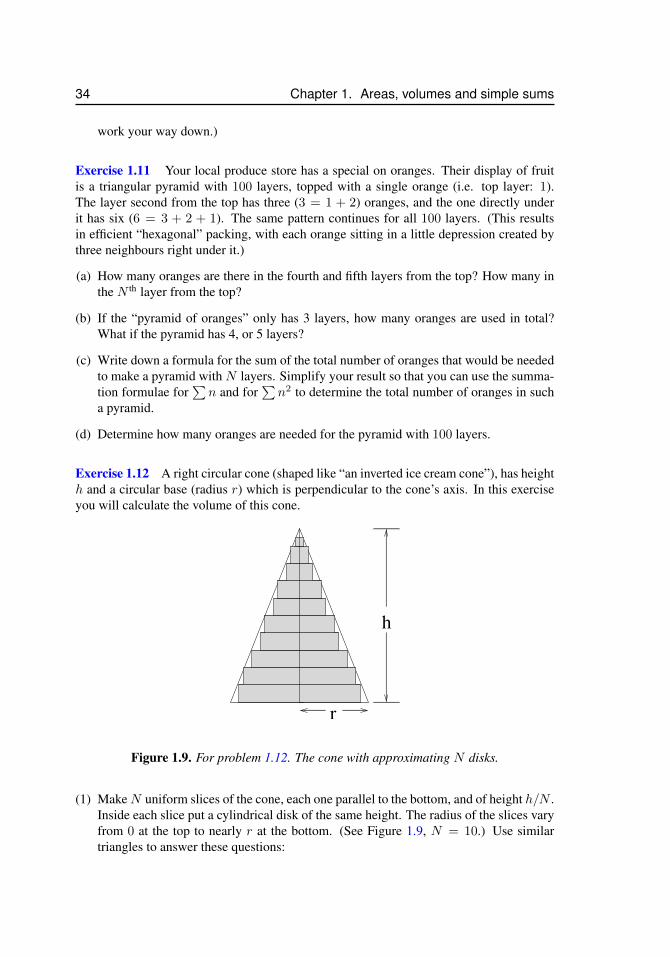
34 Chapter 1. Areas, volumes and simple sums
work your way down.)
Exercise 1.11 Your local produce store has a special on oranges. Their display of fruitis a triangular pyramid with 100 layers, topped with a single orange (i.e. top layer: 1).The layer second from the top has three (3 = 1 + 2) oranges, and the one directly underit has six (6 = 3 + 2 + 1). The same pattern continues for all 100 layers. (This resultsin efficient “hexagonal” packing, with each orange sitting in a little depression created bythree neighbours right under it.)
(a) How many oranges are there in the fourth and fifth layers from the top? How many inthe N th layer from the top?
(b) If the “pyramid of oranges” only has 3 layers, how many oranges are used in total?What if the pyramid has 4, or 5 layers?
(c) Write down a formula for the sum of the total number of oranges that would be neededto make a pyramid with N layers. Simplify your result so that you can use the summa-tion formulae for
∑n and for
∑n2 to determine the total number of oranges in such
a pyramid.
(d) Determine how many oranges are needed for the pyramid with 100 layers.
Exercise 1.12 A right circular cone (shaped like “an inverted ice cream cone”), has heighth and a circular base (radius r) which is perpendicular to the cone’s axis. In this exerciseyou will calculate the volume of this cone.
h
r
Figure 1.9. For problem 1.12. The cone with approximating N disks.
(1) MakeN uniform slices of the cone, each one parallel to the bottom, and of height h/N .Inside each slice put a cylindrical disk of the same height. The radius of the slices varyfrom 0 at the top to nearly r at the bottom. (See Figure 1.9, N = 10.) Use similartriangles to answer these questions:
1.10. Exercises 35
(a) What is the smallest disk radius other than 0?
(b) What is the radius of the kth disk?
(2) Express the total volume of the N disks as a sum and evaluate it.
(3) As N gets larger, what is the limit of this sum? (This is the volume of the cone.)
Exercise 1.13 A (finite) geometric series with k terms is a sum of the form
1 + r + r2 + r3 + ...rk−1 =k−1∑n=0
rn
and is given by the formula
S =1− rk
1− rprovided r 6= 1.
(a) This formula does not work if r = 1. Find the actual value of the series for r = 1.
(b) Express in summation notation and find the sum of the series 1+21 +22 +23 + ..+210.
(c) Express in summation notation and find the sum of the series 1 + (0.5)1 + (0.5)2 +(0.5)3 + ..(0.5)10.
Exercise 1.14 Use the sum of a geometric series to answer this question (use a calculator).
(a) Find the sum of the first 11 numbers of the form 1.1k for k = 0, 1, 2, . . .. Now find thesum of the first 21 such numbers, the first 31 such numbers, the first 41 such numbers,and the first 51 such numbers.
(b) Repeat the process but now find sums of the numbers 0.9k, k = 0, 1, 2...
(c) What do you notice about the pattern of results in part (a) and in part (b) ? Can youexplain what is happening in each of these cases and why they are different?
(d) Now consider the general problem of finding a value for the sum
N∑k=0
rk
when the number N gets larger and larger. Suggest under what circumstances this sumwill stay finite, and what value that finite sum will approach. To do this, you shouldthink about the formula for the finite geometric sum and determine how it behaves forvarious values of r as N gets very large. This idea will be very important when wediscuss infinite series.
36 Chapter 1. Areas, volumes and simple sums
Exercise 1.15 According to legend, the inventor of the game of chess (in Persia) wasoffered a prize for his clever invention. He requested payment in kind, i.e. in kernels ofgrain. He asked to be paid 1 kernel for the first square of the board, two for the second,four for the third, etc. Use a summation formula to determine the total number of kernelsof grain he would have earned in total.(Hint: a chess board has 8× 8 = 64 squares and the first square contains 20 = 1 kernel.)
Exercise 1.16 A branching colony of fungus starts as a single spore with a single segmentof filament growing out of it. This will be called generation 0. The tip of the filamentbranches, producing two new segments. Each tip then branches again and the processrepeats. Suppose there have been 10 such branching events. How many tips will there be?If each segment is the same length (1 unit), what will be the total length of all the segmentscombined after 10 branching events? (Include the length of the initial single segment inyour answer.)
Exercise 1.17 A branching plant and geometric series A plant grows by branching,starting with one segment of length `0 (in the 0’th generation). Every parent branch hasexactly two daughter branches. The length of each daughter branch is (2/5) times the lengthof the parent branch. (Your answers will be in terms of `0.)
(a) Find the total length of just the 12th generation branch segments.
(b) Find the total length of the whole structure including the original segment and all 12successive generations.
(c) Find the approximate total length of all segments in the whole structure if the plantkeeps on branching forever.
Exercise 1.18 Branching airways, continued Consider the branching airways in thelungs. Suppose that the initial bronchial segment has length `0 and radius r0. Let α andβ be the scale factors for the length and radius, respectively, of daughter branches (i.e. ina branching event, assume that `n+1 = α`n and rn+1 = βrn are the relations that linkdaughters to parent branches, and that 0 < α < 1, 0 < β < 1, li > 0, ri > 0 for all i). Letb be the average number of daughters per parent branch. Let Fn = Sn/Vn be the ratio oftotal surface area to total volume in the nth layer of the structure (i.e. for the nth generationbranches).
(a) Find Fn in terms of `0, r0, b, β, α.
(b) In the lungs, it would be reasonable to expect that the surface area to volume ratioshould increase from the initial segment down through the layers. What should be trueof the parameters for this to be the case?
Exercise 1.19 Branching lungs
(a) Consider branched airways that have the following geometric properties (Table a). Findthe total number of branch segments, the volume and the surface area of this branchedstructure. Note that a calculator will be helpful.
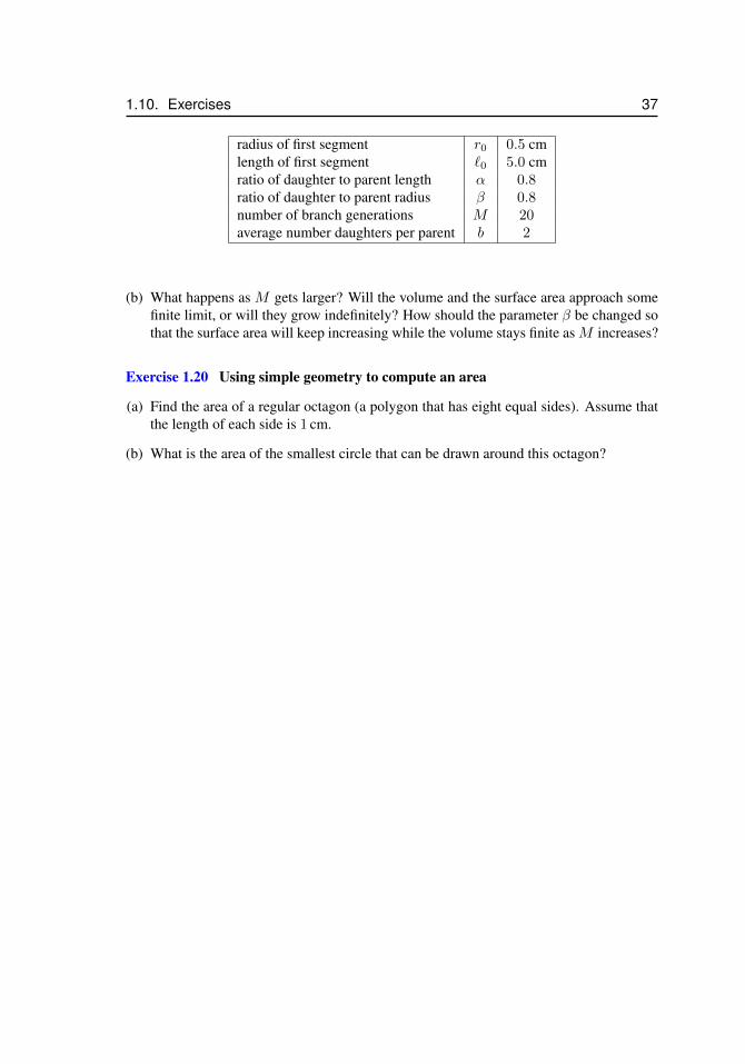
1.10. Exercises 37
radius of first segment r0 0.5 cmlength of first segment `0 5.0 cmratio of daughter to parent length α 0.8ratio of daughter to parent radius β 0.8number of branch generations M 20average number daughters per parent b 2
(b) What happens as M gets larger? Will the volume and the surface area approach somefinite limit, or will they grow indefinitely? How should the parameter β be changed sothat the surface area will keep increasing while the volume stays finite asM increases?
Exercise 1.20 Using simple geometry to compute an area
(a) Find the area of a regular octagon (a polygon that has eight equal sides). Assume thatthe length of each side is 1 cm.
(b) What is the area of the smallest circle that can be drawn around this octagon?

38 Chapter 1. Areas, volumes and simple sums

Chapter 2
Areas
2.1 Areas in the planeA long-standing problem of integral calculus is how to compute the area of a region inthe plane. This type of geometric problem formed part of the original motivation for thedevelopment of calculus techniques, and we will discuss it in many contexts in this course.We have already seen examples of the computation of areas of especially simple geometricshapes in Chapter 1. For triangles, rectangles, polygons, and circles, no advanced methods(beyond simple geometry) are needed. However, beyond these elementary shapes, suchmethods fail, and a new idea is needed. We will discuss such ideas in this chapter, and inChapter 3.
x
y
a b
A
y=f(x)
Figure 2.1. We consider the problem of determining areas of regions suchbounded by the x axis, the lines x = a and x = b and the graph of some function, y = f(x).
We now consider the problem of determining the area of a region in the plane thathas the following special properties: The region is formed by straight lines on three sides,and by a smooth curve on one of its edges, as shown in Figure 2.1. You might imaginethat the shaded portion of this figure is a plot of land bounded by fences on three sides, andby a river on the fourth side. A farmer wishing to purchase this land would want to knowexactly how large an area is being acquired. Here we set up the calculation of that area.
39
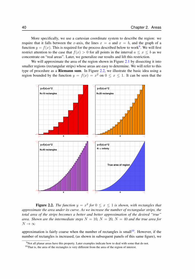
40 Chapter 2. Areas
More specifically, we use a cartesian coordinate system to describe the region: werequire that it falls between the x-axis, the lines x = a and x = b, and the graph of afunction y = f(x). This is required for the process described below to work9. We will firstrestrict attention to the case that f(x) > 0 for all points in the interval a ≤ x ≤ b as weconcentrate on “real areas”. Later, we generalize our results and lift this restriction.
We will approximate the area of the region shown in Figure 2.1 by dissecting it intosmaller regions (rectangular strips) whose areas are easy to determine. We will refer to thistype of procedure as a Riemann sum. In Figure 2.2, we illustrate the basic idea using aregion bounded by the function y = f(x) = x2 on 0 ≤ x ≤ 1. It can be seen that the
y=f(x)=x^2
x
N=10 rectangles
0.0 1.0
0.0
1.0
y=f(x)=x^2
x
N=20 rectangles
0.0 1.0
0.0
1.0
y=f(x)=x^2
x
N=40 rectangles
0.0 1.0
0.0
1.0
y=f(x)=x^2
True area of region
x
N -> infinity
0.0 1.0
0.0
1.0
Figure 2.2. The function y = x2 for 0 ≤ x ≤ 1 is shown, with rectangles thatapproximate the area under its curve. As we increase the number of rectangular strips, thetotal area of the strips becomes a better and better approximation of the desired “true”area. Shown are the intermediate steps N = 10, N = 20, N = 40 and the true area forN →∞
approximation is fairly coarse when the number of rectangles is small10. However, if thenumber of rectangles is increased, (as shown in subsequent panels of this same figure), we
9Not all planar areas have this property. Later examples indicate how to deal with some that do not.10That is, the area of the rectangles is very different from the area of the region of interest.
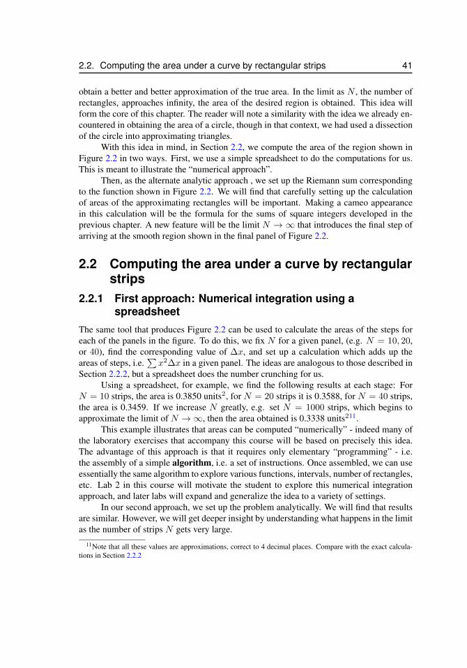
2.2. Computing the area under a curve by rectangular strips 41
obtain a better and better approximation of the true area. In the limit as N , the number ofrectangles, approaches infinity, the area of the desired region is obtained. This idea willform the core of this chapter. The reader will note a similarity with the idea we already en-countered in obtaining the area of a circle, though in that context, we had used a dissectionof the circle into approximating triangles.
With this idea in mind, in Section 2.2, we compute the area of the region shown inFigure 2.2 in two ways. First, we use a simple spreadsheet to do the computations for us.This is meant to illustrate the “numerical approach”.
Then, as the alternate analytic approach , we set up the Riemann sum correspondingto the function shown in Figure 2.2. We will find that carefully setting up the calculationof areas of the approximating rectangles will be important. Making a cameo appearancein this calculation will be the formula for the sums of square integers developed in theprevious chapter. A new feature will be the limit N → ∞ that introduces the final step ofarriving at the smooth region shown in the final panel of Figure 2.2.
2.2 Computing the area under a curve by rectangularstrips
2.2.1 First approach: Numerical integration using aspreadsheet
The same tool that produces Figure 2.2 can be used to calculate the areas of the steps foreach of the panels in the figure. To do this, we fix N for a given panel, (e.g. N = 10, 20,or 40), find the corresponding value of ∆x, and set up a calculation which adds up theareas of steps, i.e.
∑x2∆x in a given panel. The ideas are analogous to those described in
Section 2.2.2, but a spreadsheet does the number crunching for us.Using a spreadsheet, for example, we find the following results at each stage: For
N = 10 strips, the area is 0.3850 units2, for N = 20 strips it is 0.3588, for N = 40 strips,the area is 0.3459. If we increase N greatly, e.g. set N = 1000 strips, which begins toapproximate the limit of N →∞, then the area obtained is 0.3338 units211.
This example illustrates that areas can be computed “numerically” - indeed many ofthe laboratory exercises that accompany this course will be based on precisely this idea.The advantage of this approach is that it requires only elementary “programming” - i.e.the assembly of a simple algorithm, i.e. a set of instructions. Once assembled, we can useessentially the same algorithm to explore various functions, intervals, number of rectangles,etc. Lab 2 in this course will motivate the student to explore this numerical integrationapproach, and later labs will expand and generalize the idea to a variety of settings.
In our second approach, we set up the problem analytically. We will find that resultsare similar. However, we will get deeper insight by understanding what happens in the limitas the number of strips N gets very large.
11Note that all these values are approximations, correct to 4 decimal places. Compare with the exact calcula-tions in Section 2.2.2
42 Chapter 2. Areas
2.2.2 Second approach: Analytic computation using Riemannsums
In this section we consider the detailed steps involved in analytically computing the area ofthe region bounded by the function
y = f(x) = x2, 0 ≤ x ≤ 1.
By this we mean that we use “pen-and-paper” calculations, rather than computational aidsto determine that area.
We set up the rectangles (as shown in Figure 2.2, with detailed labeling in Fig-ures 2.3), determine the heights and areas of these rectangle, sum their total area, andthen determine how this value behaves as the rectangles get more numerous (and thinner).
1
y
y=f(x)=x2
f(x)
∆ x0
f(x )
y
x x x ... ...1 k−1 k N
xx0
y=f(x)
kf(x )
N
Figure 2.3. The region under the graph of y = f(x) for 0 ≤ x ≤ 1 will beapproximated by a set of N rectangles. A rectangle (shaded) has base width ∆x andheight f(x). Since 0 ≤ x ≤ 1, and the all rectangles have the same base width, it followsthat ∆x = 1/N . In the panel on the right, the coordinates of base corners and two typicalheights of the rectangles have been labeled. Here x0 = 0, xN = 1 and xk = k∆x.
The interval of interest in this problem is 0 ≤ x ≤ 1. Let us subdivide this intervalintoN equal subintervals. Then each has width 1/N . (We will refer to this width as ∆x, asshown in Figure 2.3, as it forms a difference of successive x coordinates.) The coordinatesof the endpoints of these subintervals will be labeled x0, x1, . . . , xk, . . . , xN , where thevalue x0 = 0 and xN = 1 are the endpoints of the original interval. Since the points areequally spaced, starting at x0 = 0, the coordinate xk is just k steps of size 1/N alongthe x axis, i.e. xk = k(1/N) = k/N . In the right panel of Figure 2.3, some of thesecoordinates have been labeled. For clarity, we show only the first few points, together witha representative pair xk−1 and xk inside the region.
Let us look more carefully at one of the rectangles. Suppose we look at the rectanglelabeled k. Such a representative k-th rectangle is shown shaded in Figures 2.3. The heightof this rectangle is determined by the value of the function, since one corner of the rectangleis “glued” to the curve. The choice shown in Figure 2.3 is to affix the right corner of each
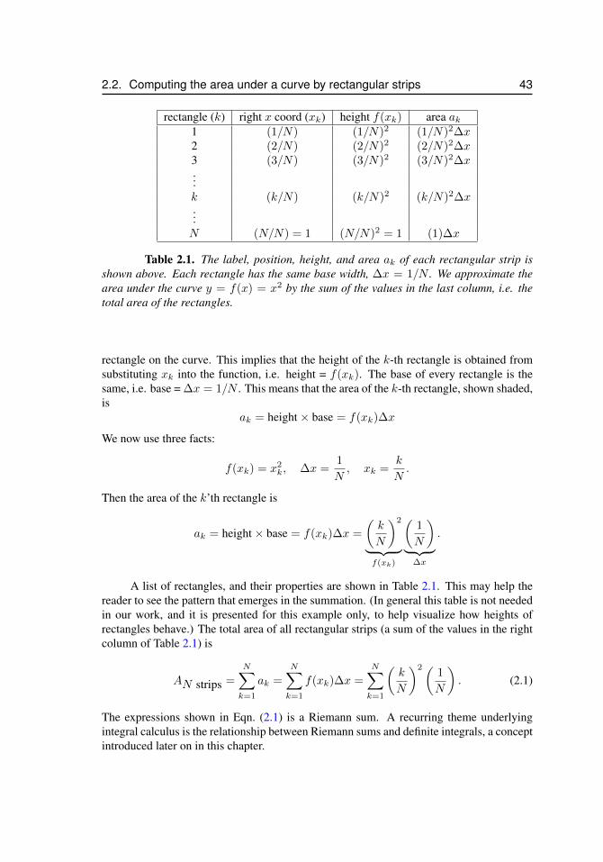
2.2. Computing the area under a curve by rectangular strips 43
rectangle (k) right x coord (xk) height f(xk) area ak1 (1/N) (1/N)2 (1/N)2∆x2 (2/N) (2/N)2 (2/N)2∆x3 (3/N) (3/N)2 (3/N)2∆x...k (k/N) (k/N)2 (k/N)2∆x...N (N/N) = 1 (N/N)2 = 1 (1)∆x
Table 2.1. The label, position, height, and area ak of each rectangular strip isshown above. Each rectangle has the same base width, ∆x = 1/N . We approximate thearea under the curve y = f(x) = x2 by the sum of the values in the last column, i.e. thetotal area of the rectangles.
rectangle on the curve. This implies that the height of the k-th rectangle is obtained fromsubstituting xk into the function, i.e. height = f(xk). The base of every rectangle is thesame, i.e. base = ∆x = 1/N . This means that the area of the k-th rectangle, shown shaded,is
ak = height× base = f(xk)∆x
We now use three facts:
f(xk) = x2k, ∆x =
1
N, xk =
k
N.
Then the area of the k’th rectangle is
ak = height× base = f(xk)∆x =
(k
N
)2
︸ ︷︷ ︸f(xk)
(1
N
)︸ ︷︷ ︸
∆x
.
A list of rectangles, and their properties are shown in Table 2.1. This may help thereader to see the pattern that emerges in the summation. (In general this table is not neededin our work, and it is presented for this example only, to help visualize how heights ofrectangles behave.) The total area of all rectangular strips (a sum of the values in the rightcolumn of Table 2.1) is
AN strips =
N∑k=1
ak =
N∑k=1
f(xk)∆x =
N∑k=1
(k
N
)2(1
N
). (2.1)
The expressions shown in Eqn. (2.1) is a Riemann sum. A recurring theme underlyingintegral calculus is the relationship between Riemann sums and definite integrals, a conceptintroduced later on in this chapter.
44 Chapter 2. Areas
We now rewrite this sum in a more convenient form so that summation formulaedeveloped in Chapter 1 can be used. In this sum, only the quantity k changes from term toterm. All other quantities are common factors, so that
AN strips =
(1
N3
) N∑k=1
k2.
The formula (1.2) for the sum of square integers can be applied to the summation, resultingin
AN strips =
(1
N3
)N(N + 1)(2N + 1)
6=
(N + 1)(2N + 1)
6N2. (2.2)
In the box below, we use Eqn. (2.2) to compute that approximate area for values of Nshown in the first three panels of Fig 2.2. Note that these are comparable to the values weobtained “numerically” in Section 2.2.1. (We plug in the value of N into (2.2) and use acalculator to obtain the results below.)
If N = 10 strips (Figure 2.2a), the width of each strip is 0.1 unit. According to equa-tion 2.2, the area of the 10 strips (shown in red) is
A10 strips =(10 + 1)(2 · 10 + 1)
6 · 102= 0.385.
If N = 20 strips (Figure 2.2b), ∆x = 1/20 = 0.05, and
A20 strips =(20 + 1)(2 · 20 + 1)
6 · 202= 0.35875.
If N = 40 strips (Figure 2.2c), ∆x = 1/40 = 0.025 and
A40 strips =(40 + 1)(2 · 40 + 1)
6 · 402= 0.3459375.
We will define the true area under the graph of the function y = f(x) over the giveninterval to be:
A = limN→∞
AN strips.
This means that the true area is obtained by letting the number of rectangular strips, N , getvery large, (while the width of each one, ∆x = 1/N gets very small.)
In the example discussed in this section, the true area is found by taking the limit asN gets large in equation (2.2), i.e.,
A = limN→∞
(1
N2
)(N + 1)(2N + 1)
6=
1
6limN→∞
(N + 1)(2N + 1)
N2.
To evaluate this limit, note that when N gets very large, we can use the approximations,(N + 1) ≈ N and (2N + 1) ≈ 2N so that (simplifying and cancelling common factors)
limN→∞
(N + 1)(2N + 1)
N2= limN→∞
(N)
N
(2N)
N= 2.
2.3. The area of a leaf 45
The result is:A =
1
6(2) =
1
3≈ 0.333. (2.3)
Thus, the true area of the region (Figure 2.2d) is is 1/3 units2.
2.2.3 CommentsMany student who have had calculus before in highschool, ask “why do we bother withsuch tedious calculations, when we could just use integration?”. Indeed, our developmentof Riemann sums foreshadows and anticipates the idea of a definite integral, and in shortorder, some powerful techniques will help to shortcut such technical calculations. Thereare two reasons why we linger on Riemann sums. First, in order to understand integrationadequately, we must understand the underlying “technology” and concepts; this provesvital in understanding how to use the methods, and when things can go wrong. It also helpsto understand what integrals represent in applications that occur later on. Second, eventhough we will shortly have better tools for analytical calculations, the ideas of setting uparea approximations using rectangular strips is very similar to the way that the spreadsheetcomputations are designed. (However, the summation is handled automatically using thespreadsheet, and no “formulae” are needed.) In Section 2.2.1, we gave only few details ofthe steps involved. The student will find that understanding the ideas of Section 2.2.2 willgo hand-in-hand with understanding the numerical approach of Section 2.2.1.
The ideas outlined above can be applied to more complicated situations. In the nextsection we consider a practical problem in which a similar calculation is carried out.
2.3 The area of a leafLeaves act as solar energy collectors for plants. Hence, their surface area is an importantproperty. In this section we use our techniques to determine the area of a rhododendronleaf, shown in Figure 2.4. For simplicity of treatment, we will first consider a functiondesigned to mimic the shape of the leaf in a simple system of units: we will scale distancesby the length of the leaf, so that its profile is contained in the interval 0 ≤ x ≤ 1. We laterask how to modify this treatment to describe similarly curved leaves of arbitrary length andwidth, and leaves that are less symmetric. As shown in Figure 2.4, a simple parabola, ofthe form
y = f(x) = x(1− x),
provides a convenient approximation to the top edge of the leaf. To check that this is thecase, we observe that at x = 0 and x = 1, the curve intersects the x axis. At 0 < x < 1,the curve is above the axis. Thus, the area between this curve and the x axis, is one half ofthe leaf area.
We set up the computation of approximating rectangular strips as before, by sub-dividing the interval of interest into N rectangular strips. We can set up the calculationsystematically, as follows:
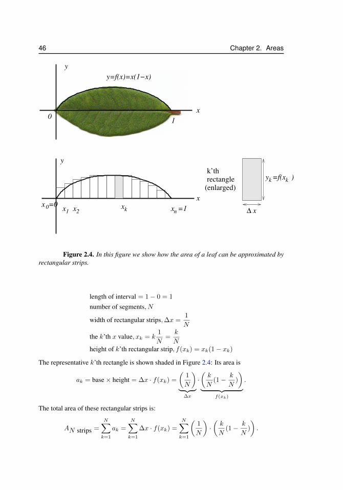
46 Chapter 2. Areas
1
x
y
0
y=f(x)=x(1−x)
x
y
x =00 x1 x2 x =1n
ky =f(x )k
∆ x
k’th rectangle
(enlarged)
xk
Figure 2.4. In this figure we show how the area of a leaf can be approximated byrectangular strips.
length of interval = 1− 0 = 1
number of segments, N
width of rectangular strips,∆x =1
N
the k’th x value, xk = k1
N=
k
Nheight of k’th rectangular strip, f(xk) = xk(1− xk)
The representative k’th rectangle is shown shaded in Figure 2.4: Its area is
ak = base× height = ∆x · f(xk) =
(1
N
)︸ ︷︷ ︸
∆x
·(k
N(1− k
N)
)︸ ︷︷ ︸
f(xk)
.
The total area of these rectangular strips is:
AN strips =
N∑k=1
ak =
N∑k=1
∆x · f(xk) =
N∑k=1
(1
N
)·(k
N(1− k
N)
).

2.4. Area under an exponential curve 47
Simplifying the result (so we can use summation formulae) leads to:
AN strips =
(1
N
) N∑k=1
(k
N(1− k
N)
)=
(1
N2
) N∑k=1
k −(
1
N3
) N∑k=1
k2.
Using the summation formulae (1.4) and(1.2) from Chapter 1 results in:
AN strips =
(1
N2
)(N(N + 1)
2
)−(
1
N3
)((2N + 1)N(N + 1)
6
).
Simplifying, and regrouping terms, we get
AN strips =1
2
((N + 1)
N
)− 1
6
((2N + 1)(N + 1)
N2
).
This is the area for a finite number, N , of rectangular strips. As before, the true area isobtained as the limit as N goes to infinity, i.e. A = limN→∞AN strips. We obtain:
A = limN→∞
1
2
((N + 1)
N
)− limN→∞
1
6
((2N + 1)(N + 1)
N2
)=
1
2− 1
6· 2 =
1
6.
Taking the limit leads to
A =1
2− 1
6· 2 =
1
2− 1
3=
1
6.
Thus the area of the entire leaf (twice this area) is 1/3.
Remark:
The function in this example can be written as y = x − x2. For part of this expression,we have seen a similar calculation in Section 2.2. This example illustrates an importantproperty of sums, namely the fact that we can rearrange the terms into simpler expressionsthat can be summed individually.
In the homework problems accompanying this chapter, we investigate how to de-scribe leaves with arbitrary lengths and widths, as well as leaves with shapes that are ta-pered, broad, or less symmetric than the current example.
2.4 Area under an exponential curveIn the precious examples, we considered areas under curves described by a simple quadraticfunctions. Each of these led to calculations in which sums of integers or square integersappeared. Here we demonstrate an example in which a geometric sum will be used. Recallthat we derived Eqn. (1.5) in Chapter 1, for a finite geometric sum.
We will find the area under the graph of the function y = f(x) = e2x over theinterval between x = 0 and x = 2. In evaluating a limit in this example, we will also usethe fact that the exponential function has a linear approximation as follows:
ez ≈ 1 + z
48 Chapter 2. Areas
(See Linear Approximations in an earlier calculus course.)As before, we subdivide the interval into N pieces, each of width 2/N . Proceeding
systematically as before, we write
length of interval = 2− 0 = 2
number of segments = N
width of rectangular strips,∆x =2
N
the k’th x value, xk = k2
N=
2k
N
height of k’th rectangular strip, f(xk) = e2xk = e2(2k/N) = e4k/N
We observe that the length of the interval (here 2) has affected the details of the calculation.As before, the area of the k’th rectangle is
ak = base× height = ∆x× f(xk) =
(2
N
)e4k/N ,
and the total area of all the rectangles is
AN strips =
(2
N
) N∑k=1
e4k/N =
(2
N
) N∑k=1
rk =
(2
N
)( N∑k=0
rk − r0
),
where r = e4/N . This is a finite geometric series. Because the series starts with k = 1 andnot with k = 0, the sum is
AN strips =
(2
N
)[(1− rN+1)
(1− r)− 1
].
After some simplification and using r = e4/N , we find that
AN strips =
(2
N
)e4/N 1− e4
1− e4/N= 2
1− e4
N(e−4/N − 1).
We need to determine what happens whenN gets very large. We can use the linear approx-imation
e−4/N ≈ 1− 4/N
to evaluate the limit of the term in the denominator, and we find that
A = limN→∞
21− e4
N(e−4/N − 1)= limN→∞
21− e4
−N(1 + 4/N − 1)= 2
e4 − 1
4≈ 26.799.
2.5 Extensions and other examplesMore general interval
To calculate the area under the curve y = f(x) = x2 over the interval 2 ≤ x ≤ 5 usingN rectangles, the width of each one would be ∆x = (5 − 2)/N = 3/N , (i.e., length of

2.6. The definite integral 49
interval divided by N). Since the interval starts at x0 = 2, and increments in units of (3/N),the k’th coordinate is xk = 2 + k(3/N) = 2 + (3k/N). The area of the k’th rectangle isthen AK = f(xk) × ∆x = [(2 + (3k/N))2](3/N), and this is to be summed over k. Asimilar algebraic simplification, summation formulae, and limit is needed to calculate thetrue area.
Other examples
At the end of this chapter we discuss a number of other examples with several modifi-cations: First, we show how to set up a Riemann sum for a more complicated quadraticfunction on a general interval, a ≤ x ≤ b. Second, we show how Riemann sums can be setup for left, rather than right endpoint approximations. The results are entirely analogous.
2.6 The definite integralWe now introduce a central concept that will form an important theme in this course, thatof the definite integral. We begin by defining a new piece of notation relevant to the topicin this chapter, namely the area associated with the graph of a function. For a function y =
x
y
a b
A
y=f(x)
Figure 2.5. The shaded area A corresponds to the definite integral I of the func-tion f(x) over the interval a ≤ x ≤ b.
f(x) > 0 that is bounded and continuous12 on an interval [a, b] (also written a ≤ x ≤ b),we define the definite integral,
I =
∫ b
a
f(x) dx (2.4)
to be the area A of the region under the graph of the function between the endpoints a andb. See Figure 2.5.
2.6.1 Remarks1. The definite integral is a number.
12A function is said to be bounded if its graph stays between some pair of horizontal lines. It is continuous ifthere are no “breaks” in its graph.
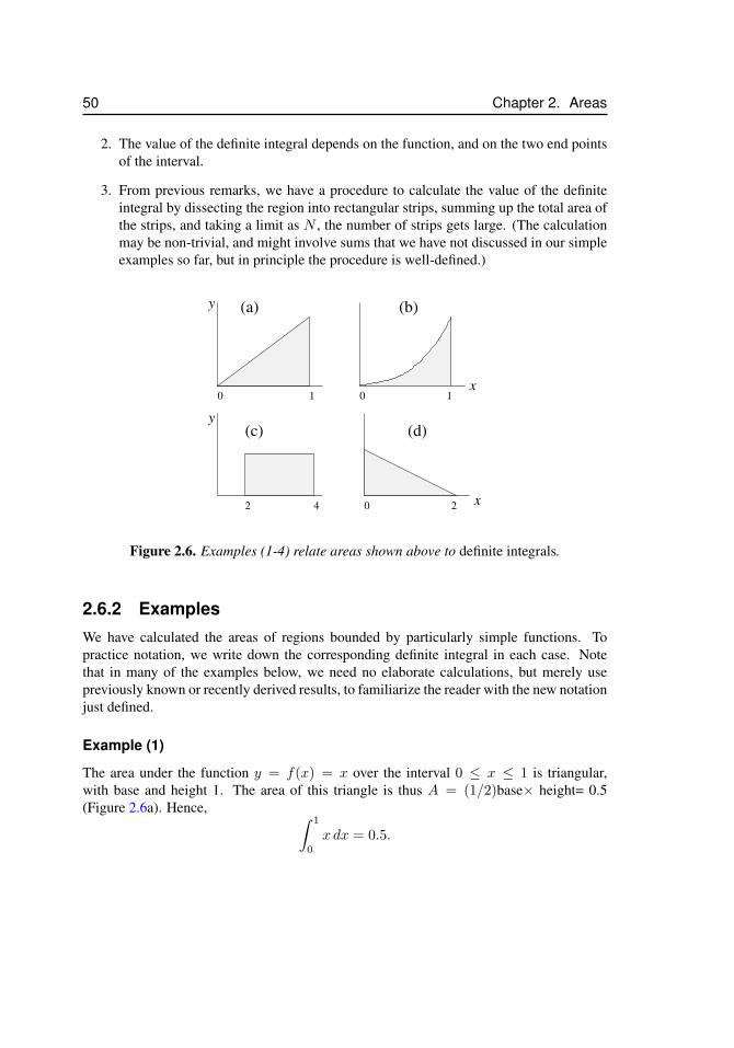
50 Chapter 2. Areas
2. The value of the definite integral depends on the function, and on the two end pointsof the interval.
3. From previous remarks, we have a procedure to calculate the value of the definiteintegral by dissecting the region into rectangular strips, summing up the total area ofthe strips, and taking a limit as N , the number of strips gets large. (The calculationmay be non-trivial, and might involve sums that we have not discussed in our simpleexamples so far, but in principle the procedure is well-defined.)
(a) (b)
(c) (d)
0 1 0
2 4 0 2
1
x
x
y
y
Figure 2.6. Examples (1-4) relate areas shown above to definite integrals.
2.6.2 ExamplesWe have calculated the areas of regions bounded by particularly simple functions. Topractice notation, we write down the corresponding definite integral in each case. Notethat in many of the examples below, we need no elaborate calculations, but merely usepreviously known or recently derived results, to familiarize the reader with the new notationjust defined.
Example (1)
The area under the function y = f(x) = x over the interval 0 ≤ x ≤ 1 is triangular,with base and height 1. The area of this triangle is thus A = (1/2)base× height= 0.5(Figure 2.6a). Hence, ∫ 1
0
x dx = 0.5.
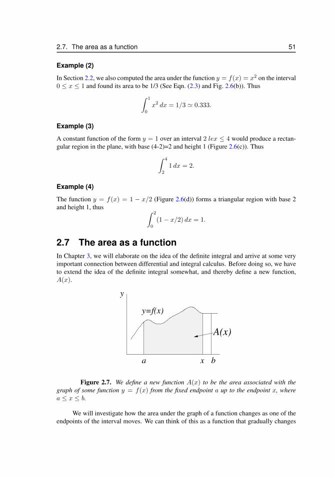
2.7. The area as a function 51
Example (2)
In Section 2.2, we also computed the area under the function y = f(x) = x2 on the interval0 ≤ x ≤ 1 and found its area to be 1/3 (See Eqn. (2.3) and Fig. 2.6(b)). Thus∫ 1
0
x2 dx = 1/3 ' 0.333.
Example (3)
A constant function of the form y = 1 over an interval 2 lex ≤ 4 would produce a rectan-gular region in the plane, with base (4-2)=2 and height 1 (Figure 2.6(c)). Thus∫ 4
2
1 dx = 2.
Example (4)
The function y = f(x) = 1 − x/2 (Figure 2.6(d)) forms a triangular region with base 2and height 1, thus ∫ 2
0
(1− x/2) dx = 1.
2.7 The area as a functionIn Chapter 3, we will elaborate on the idea of the definite integral and arrive at some veryimportant connection between differential and integral calculus. Before doing so, we haveto extend the idea of the definite integral somewhat, and thereby define a new function,A(x).
y
a
y=f(x)
A(x)
bx
Figure 2.7. We define a new function A(x) to be the area associated with thegraph of some function y = f(x) from the fixed endpoint a up to the endpoint x, wherea ≤ x ≤ b.
We will investigate how the area under the graph of a function changes as one of theendpoints of the interval moves. We can think of this as a function that gradually changes
52 Chapter 2. Areas
(i.e. the area accumulates) as we sweep across the interval (a, b) from left to right inFigure 2.1. The function A(x) represents the area of the region shown in Figure 2.7.
Extending our definition of the definite integral, we might be tempted to use thenotation
A(x) =
∫ x
a
f(x) dx.
However, there is a slight problem with this notation: the symbol x is used in slightlyconfusing ways, both as the argument of the function and as the variable endpoint of theinterval. To avoid possible confusion, we will prefer the notation
A(x) =
∫ x
a
f(s) ds.
(or some symbol other than s used as a placeholder instead of x.)An analogue already seen is the sum
N∑k=1
k2
where N denotes the “end” of the sum, and k keeps track of where we are in the processof summation. The symbol s, sometimes called a “dummy variable” is analogous to thesummation symbol k.
In the upcoming Chapter 3, we will investigate properties of this new “area function”A(x) defined above. This will lead us to the Fundamental Theorem of Calculus, and willprovide new and powerful tools to replace the dreary summations that we had to performin much of Chapter 2. Indeed, we are about to discover the amazing connection between afunction, the area A(x) under its curve, and the derivative of A(x).
2.8 SummaryIn this chapter, we showed how to calculate the area of a region in the plane that is boundedby the x axis, two lines of the form x = a and x = b, and the graph of a positive functiony = f(x). We also introduced the terminology “definite integral” (Section 2.6) and thenotation (2.4) to represent that area.
One of our main efforts here focused on how to actually compute that area by thefollowing set of steps:
• Subdivide the interval [a, b] into smaller intervals (width ∆x).
• Construct rectangles whose heights approximate the height of the function above thegiven interval.
• Add up the areas of these approximating rectangles. (Here we often used summationformulae from Chapter 1.) The resulting expression, such as Eqn. (2.1), for example,was denoted a Riemann sum.
• Find out what happens to this total area in the limit when the width ∆x goes to zero(or, in other words, when the number of rectangles N goes to infinity).
2.9. Optional Material 53
We showed both the analytic approach, using Riemann sums and summation formu-lae to find areas, as well as numerical approximations using a spreadsheet tool to arrive atsimilar results. We then used a variety of examples to illustrate the concepts and arrive atcomputed areas.
As a final important point, we noted that the area “under the graph of a function” canitself be considered a function. This idea will emerge as particularly important and will leadus to the key concept linking the geometric concept of areas with the analytic propertiesof antiderivatives. We shall see this link in the Fundamental Theorem of Calculus, inChapter 3.
2.9 Optional MaterialWe take up some issues here that were not yet considered in the context of our examples ofRiemann sums. First, we consider an arbitrary interval a ≤ x ≤ b. Then we comment onother ways of constructing the rectangular strip approximation (that eventually lead to thesame limit when the true area is computed.)
2.9.1 Riemann sums over a general interval: a ≤ x ≤ b
Find the area under the graph of the function
y = f(x) = x2 + 2x+ 1 a ≤ x ≤ b.
Here the interval is a ≤ x ≤ b. Let us leave the values of a, b general for a moment, andconsider how the calculation is set up in this case.13 Then we have
length of interval: b− anumber of segments: N
width of rectangular strips: ∆x =b− aN
the k’th x value: xk = a+ k(b− a)
N
height of k’th rectangular strip: f(xk) = x2k + 2xk + 1
Combining the last two steps, the height of rectangle k is:
f(xk) =
(a+
k(b− a)
N
)2
+ 2
(a+
k(b− a)
N
)+ 1
and its area is
ak = f(xk)×∆x = f(xk)×(b− aN
).
We use the last two equations to express ak in terms of k (and the quantities a, b,N ), thensum over k as before (A = ΣAk). Some algebra is needed to simplify the sums so that
13Example by Lu Fan.
54 Chapter 2. Areas
summation formulae can be applied. The details are left as an exercise for the reader (seeproblem sets). Evaluating the limit N →∞, we finally obtain
A = limN→∞
N∑k=1
ak = (a+ 1)2(b− a) + (a+ 1)(b− a)2 +(b− a)3
3.
as the area under the function f(x) = x2 + 2x + 1, over the interval a ≤ x ≤ b. Observethat the solution depends on a, and b. (The endpoints of the interval influence the totalarea under the curve.) For example, if the given interval happens to be 2 ≤ x ≤ 4. Then,substituting a = 2, b = 4 into the above result for A, leads to
A = (2 + 1)2(4− 2) + (2 + 1)(4− 2)2 +4− 2
3= 18 + 12 +
2
3=
32
3
In the next chapter, we will show that the tools of integration will lead to the same conclu-sion.
2.9.2 Riemann sums using left (rather than right) endpointsSo far, we used the right endpoint of each rectangular strip to assign its height using thegiven function (see Figs. 2.2, 2.3, 2.4). Restated, we “glued” the top right corner of therectangle to the graph of the function. This is the so called right endpoint approxima-tion. We can just as well use the left corners of the rectangles to assign their heights (leftendpoint approximation). A comparison of these for the function y = f(x) = x2 isshown in Figs. 2.8 and 2.9. In the case of the left endpoint approximation, we evaluate theheights of the rectangles starting at x0 (instead of x1, and ending at xN−1 (instead of xN ).There are still N rectangles. To compare, sum of areas of the rectangles in the left versusthe right endpoint approximation is
Right endpoints: AN strips =
N∑k=1
f(xk)∆x.
Left endpoints: AN strips =
N−1∑k=0
f(xk)∆x.
Example: We here look again at a simple example, using the quadratic function,
f(x) = x2, 0 ≤ x ≤ 1,
We now compare the right and left endpoint approximation. These are shown in panels ofFigure 2.9. Note that
∆x =1
N, xk =
k
N,
The area of the k’th rectangle is
ak = f(xk)×∆x = (k/N)2
(1/N) ,
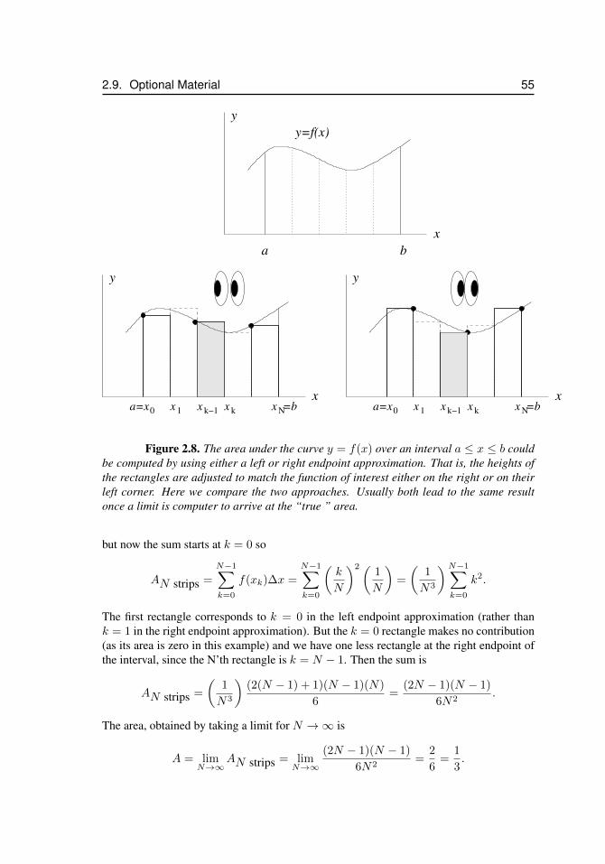
2.9. Optional Material 55
y=f(x)
a b
x
y
x x x1
a=x0 k−1 k N
x =b x x x1
a=x0 k−1 k N
x =bx
y
x
y
Figure 2.8. The area under the curve y = f(x) over an interval a ≤ x ≤ b couldbe computed by using either a left or right endpoint approximation. That is, the heights ofthe rectangles are adjusted to match the function of interest either on the right or on theirleft corner. Here we compare the two approaches. Usually both lead to the same resultonce a limit is computer to arrive at the “true ” area.
but now the sum starts at k = 0 so
AN strips =
N−1∑k=0
f(xk)∆x =
N−1∑k=0
(k
N
)2(1
N
)=
(1
N3
)N−1∑k=0
k2.
The first rectangle corresponds to k = 0 in the left endpoint approximation (rather thank = 1 in the right endpoint approximation). But the k = 0 rectangle makes no contribution(as its area is zero in this example) and we have one less rectangle at the right endpoint ofthe interval, since the N’th rectangle is k = N − 1. Then the sum is
AN strips =
(1
N3
)(2(N − 1) + 1)(N − 1)(N)
6=
(2N − 1)(N − 1)
6N2.
The area, obtained by taking a limit for N →∞ is
A = limN→∞
AN strips = limN→∞
(2N − 1)(N − 1)
6N2=
2
6=
1
3.
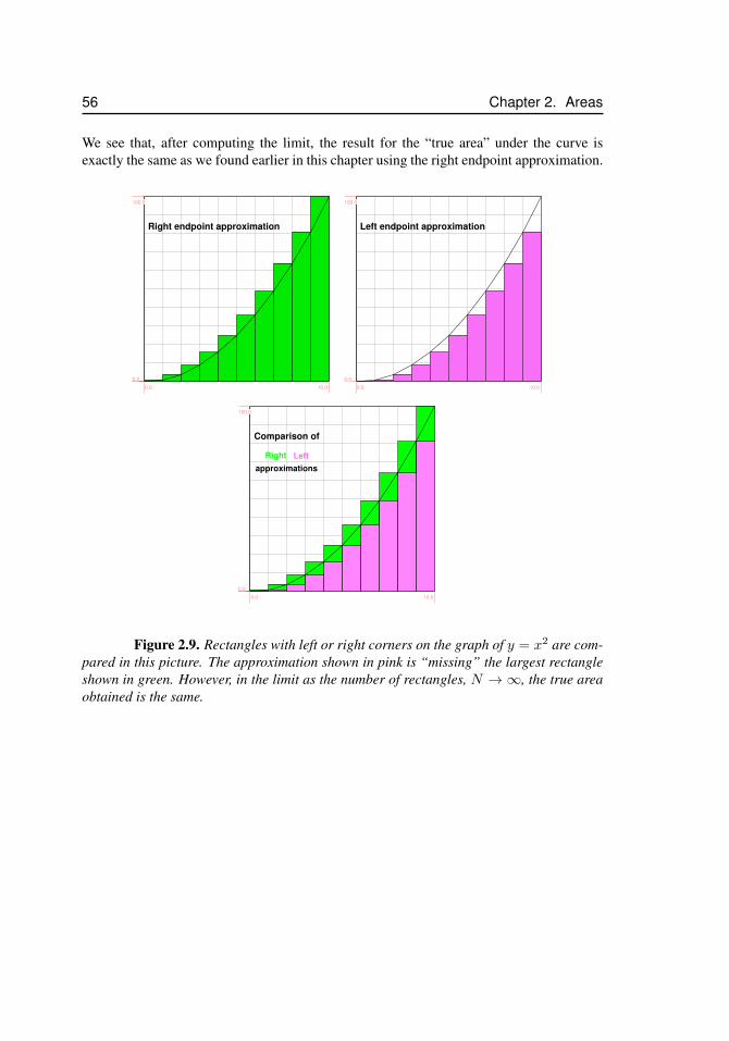
56 Chapter 2. Areas
We see that, after computing the limit, the result for the “true area” under the curve isexactly the same as we found earlier in this chapter using the right endpoint approximation.
Right endpoint approximation
0.0 10.0
0.0
100.0
Left endpoint approximation
0.0 10.0
0.0
100.0
Comparison of
LeftRight
approximations
0.0 10.0
0.0
100.0
Figure 2.9. Rectangles with left or right corners on the graph of y = x2 are com-pared in this picture. The approximation shown in pink is “missing” the largest rectangleshown in green. However, in the limit as the number of rectangles, N → ∞, the true areaobtained is the same.
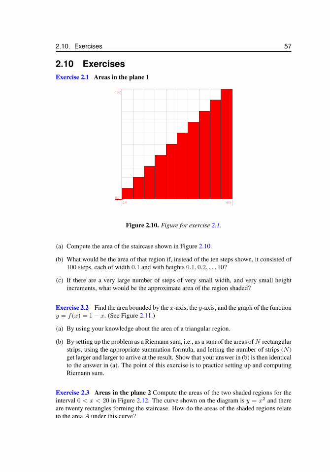
2.10. Exercises 57
2.10 ExercisesExercise 2.1 Areas in the plane 1
0.0 10.00.0
10.0
Figure 2.10. Figure for exercise 2.1.
(a) Compute the area of the staircase shown in Figure 2.10.
(b) What would be the area of that region if, instead of the ten steps shown, it consisted of100 steps, each of width 0.1 and with heights 0.1, 0.2, . . . 10?
(c) If there are a very large number of steps of very small width, and very small heightincrements, what would be the approximate area of the region shaded?
Exercise 2.2 Find the area bounded by the x-axis, the y-axis, and the graph of the functiony = f(x) = 1− x. (See Figure 2.11.)
(a) By using your knowledge about the area of a triangular region.
(b) By setting up the problem as a Riemann sum, i.e., as a sum of the areas ofN rectangularstrips, using the appropriate summation formula, and letting the number of strips (N )get larger and larger to arrive at the result. Show that your answer in (b) is then identicalto the answer in (a). The point of this exercise is to practice setting up and computingRiemann sum.
Exercise 2.3 Areas in the plane 2 Compute the areas of the two shaded regions for theinterval 0 < x < 20 in Figure 2.12. The curve shown on the diagram is y = x2 and thereare twenty rectangles forming the staircase. How do the areas of the shaded regions relateto the area A under this curve?
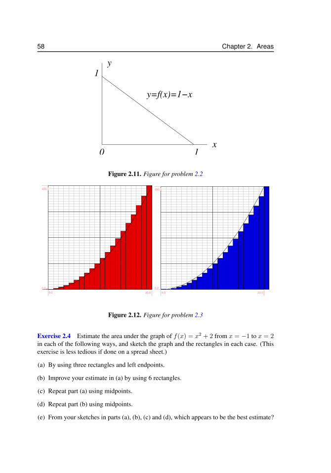
58 Chapter 2. Areas
0x
y
y=f(x)=1−x
1
1
Figure 2.11. Figure for problem 2.2
0.0 20.00.0
400.0
0.0 20.00.0
400.0
Figure 2.12. Figure for problem 2.3
Exercise 2.4 Estimate the area under the graph of f(x) = x2 + 2 from x = −1 to x = 2in each of the following ways, and sketch the graph and the rectangles in each case. (Thisexercise is less tedious if done on a spread sheet.)
(a) By using three rectangles and left endpoints.
(b) Improve your estimate in (a) by using 6 rectangles.
(c) Repeat part (a) using midpoints.
(d) Repeat part (b) using midpoints.
(e) From your sketches in parts (a), (b), (c) and (d), which appears to be the best estimate?
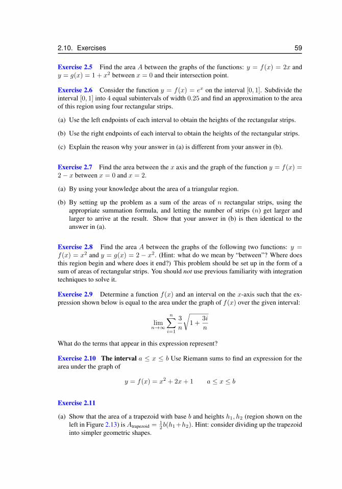
2.10. Exercises 59
Exercise 2.5 Find the area A between the graphs of the functions: y = f(x) = 2x andy = g(x) = 1 + x2 between x = 0 and their intersection point.
Exercise 2.6 Consider the function y = f(x) = ex on the interval [0, 1]. Subdivide theinterval [0, 1] into 4 equal subintervals of width 0.25 and find an approximation to the areaof this region using four rectangular strips.
(a) Use the left endpoints of each interval to obtain the heights of the rectangular strips.
(b) Use the right endpoints of each interval to obtain the heights of the rectangular strips.
(c) Explain the reason why your answer in (a) is different from your answer in (b).
Exercise 2.7 Find the area between the x axis and the graph of the function y = f(x) =2− x between x = 0 and x = 2.
(a) By using your knowledge about the area of a triangular region.
(b) By setting up the problem as a sum of the areas of n rectangular strips, using theappropriate summation formula, and letting the number of strips (n) get larger andlarger to arrive at the result. Show that your answer in (b) is then identical to theanswer in (a).
Exercise 2.8 Find the area A between the graphs of the following two functions: y =f(x) = x2 and y = g(x) = 2 − x2. (Hint: what do we mean by “between”? Where doesthis region begin and where does it end?) This problem should be set up in the form of asum of areas of rectangular strips. You should not use previous familiarity with integrationtechniques to solve it.
Exercise 2.9 Determine a function f(x) and an interval on the x-axis such that the ex-pression shown below is equal to the area under the graph of f(x) over the given interval:
limn→∞
n∑i=1
3
n
√1 +
3i
n
What do the terms that appear in this expression represent?
Exercise 2.10 The interval a ≤ x ≤ b Use Riemann sums to find an expression for thearea under the graph of
y = f(x) = x2 + 2x+ 1 a ≤ x ≤ b
Exercise 2.11
(a) Show that the area of a trapezoid with base b and heights h1, h2 (region shown on theleft in Figure 2.13) isAtrapezoid = 1
2b(h1 +h2). Hint: consider dividing up the trapezoidinto simpler geometric shapes.
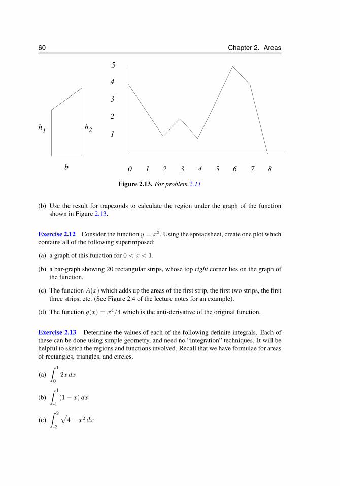
60 Chapter 2. Areas
5
h1
b 0 1 2 3 4 5 6 7 8
1
2
3
4
h2
Figure 2.13. For problem 2.11
(b) Use the result for trapezoids to calculate the region under the graph of the functionshown in Figure 2.13.
Exercise 2.12 Consider the function y = x3.Using the spreadsheet, create one plot whichcontains all of the following superimposed:
(a) a graph of this function for 0 < x < 1.
(b) a bar-graph showing 20 rectangular strips, whose top right corner lies on the graph ofthe function.
(c) The functionA(x) which adds up the areas of the first strip, the first two strips, the firstthree strips, etc. (See Figure 2.4 of the lecture notes for an example).
(d) The function g(x) = x4/4 which is the anti-derivative of the original function.
Exercise 2.13 Determine the values of each of the following definite integrals. Each ofthese can be done using simple geometry, and need no “integration” techniques. It will behelpful to sketch the regions and functions involved. Recall that we have formulae for areasof rectangles, triangles, and circles.
(a)∫ 1
0
2x dx
(b)∫ 1
-1(1− x) dx
(c)∫ 2
-2
√4− x2 dx
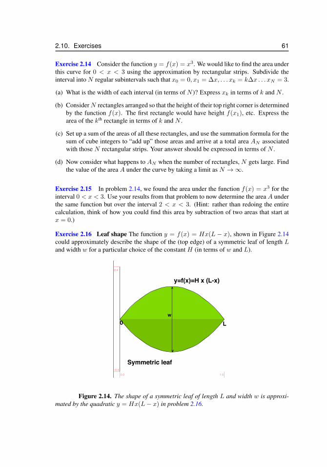
2.10. Exercises 61
Exercise 2.14 Consider the function y = f(x) = x3. We would like to find the area underthis curve for 0 < x < 3 using the approximation by rectangular strips. Subdivide theinterval into N regular subintervals such that x0 = 0, x1 = ∆x, . . . xk = k∆x . . . xN = 3.
(a) What is the width of each interval (in terms of N )? Express xk in terms of k and N .
(b) ConsiderN rectangles arranged so that the height of their top right corner is determinedby the function f(x). The first rectangle would have height f(x1), etc. Express thearea of the kth rectangle in terms of k and N .
(c) Set up a sum of the areas of all these rectangles, and use the summation formula for thesum of cube integers to “add up” those areas and arrive at a total area AN associatedwith those N rectangular strips. Your answer should be expressed in terms of N .
(d) Now consider what happens to AN when the number of rectangles, N gets large. Findthe value of the area A under the curve by taking a limit as N →∞.
Exercise 2.15 In problem 2.14, we found the area under the function f(x) = x3 for theinterval 0 < x < 3. Use your results from that problem to now determine the area A underthe same function but over the interval 2 < x < 3. (Hint: rather than redoing the entirecalculation, think of how you could find this area by subtraction of two areas that start atx = 0.)
Exercise 2.16 Leaf shape The function y = f(x) = Hx(L − x), shown in Figure 2.14could approximately describe the shape of the (top edge) of a symmetric leaf of length Land width w for a particular choice of the constant H (in terms of w and L).
Symmetric leaf
y=f(x)=H x (L-x)
V
^
w
L0
0.0 1.0-0.4
0.4
Figure 2.14. The shape of a symmetric leaf of length L and width w is approxi-mated by the quadratic y = Hx(L− x) in problem 2.16.
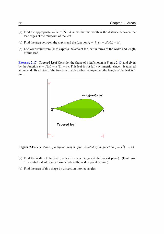
62 Chapter 2. Areas
(a) Find the appropriate value of H . Assume that the width is the distance between theleaf edges at the midpoint of the leaf.
(b) Find the area between the x axis and the function y = f(x) = Hx(L− x).
(c) Use your result from (a) to express the area of the leaf in terms of the width and lengthof this leaf.
Exercise 2.17 Tapered Leaf Consider the shape of a leaf shown in Figure 2.15, and givenby the function y = f(x) = x2(1− x). This leaf is not fully symmetric, since it is taperedat one end. By choice of the function that describes its top edge, the length of the leaf is 1unit.
Tapered leaf
y=f(x)=x^2 (1-x)
0 1
0.0 1.0-0.4
0.4
Figure 2.15. The shape of a tapered leaf is approximated by the function y = x2(1− x).
(a) Find the width of the leaf (distance between edges at the widest place). (Hint: usedifferential calculus to determine where the widest point occurs.)
(b) Find the area of this shape by dissection into rectangles.
Chapter 3
The FundamentalTheorem of Calculus
In this chapter we will formulate one of the most important results of calculus, the Funda-mental Theorem. This result will link together the notions of an integral and a derivative.Using this result will allow us to replace the technical calculations of Chapter 2 by muchsimpler procedures involving antiderivatives of a function.
3.1 The definite integralIn Chapter 2, we defined the definite integral, I , of a function f(x) > 0 on an interval [a, b]as the area under the graph of the function over the given interval a ≤ x ≤ b. We used thenotation
I =
∫ b
a
f(x)dx
to represent that quantity. We also set up a technique for computing areas: the procedurefor calculating the value of I is to write down a sum of areas of rectangular strips and tocompute a limit as the number of strips increases:
I =
∫ b
a
f(x)dx = limN→∞
N∑k=1
f(xk)∆x, (3.1)
where N is the number of strips used to approximate the region, k is an index associatedwith the k’th strip, and ∆x = xk+1 − xk is the width of the rectangle. As the number ofstrips increases (N →∞), and their width decreases (∆x→ 0), the sum becomes a betterand better approximation of the true area, and hence, of the definite integral, I . Exampleof such calculations (tedious as they were) formed the main theme of Chapter 2 .
We can generalize the definite integral to include functions that are not strictly pos-itive, as shown in Figure 3.1. To do so, note what happens as we incorporate strips cor-responding to regions of the graph below the x axis: These are associated with negativevalues of the function, so that the quantity f(xk)∆x in the above sum would be negativefor each rectangle in the “negative” portions of the function. This means that regions of thegraph below the x axis will contribute negatively to the net value of I .
63
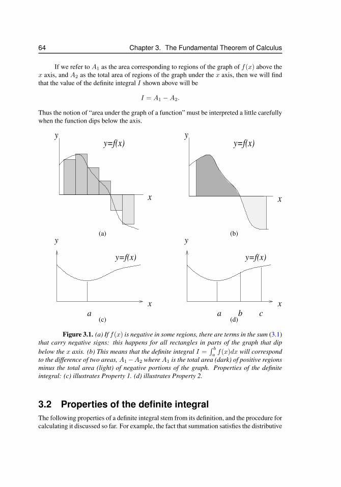
64 Chapter 3. The Fundamental Theorem of Calculus
If we refer to A1 as the area corresponding to regions of the graph of f(x) above thex axis, and A2 as the total area of regions of the graph under the x axis, then we will findthat the value of the definite integral I shown above will be
I = A1 −A2.
Thus the notion of “area under the graph of a function” must be interpreted a little carefullywhen the function dips below the axis.
x
yy=f(x)
x
yy=f(x)
(a) (b)
x
y
a
y=f(x)
x
y
a
y=f(x)
b c(c) (d)
Figure 3.1. (a) If f(x) is negative in some regions, there are terms in the sum (3.1)that carry negative signs: this happens for all rectangles in parts of the graph that dipbelow the x axis. (b) This means that the definite integral I =
∫ baf(x)dx will correspond
to the difference of two areas, A1−A2 where A1 is the total area (dark) of positive regionsminus the total area (light) of negative portions of the graph. Properties of the definiteintegral: (c) illustrates Property 1. (d) illustrates Property 2.
3.2 Properties of the definite integralThe following properties of a definite integral stem from its definition, and the procedure forcalculating it discussed so far. For example, the fact that summation satisfies the distributive
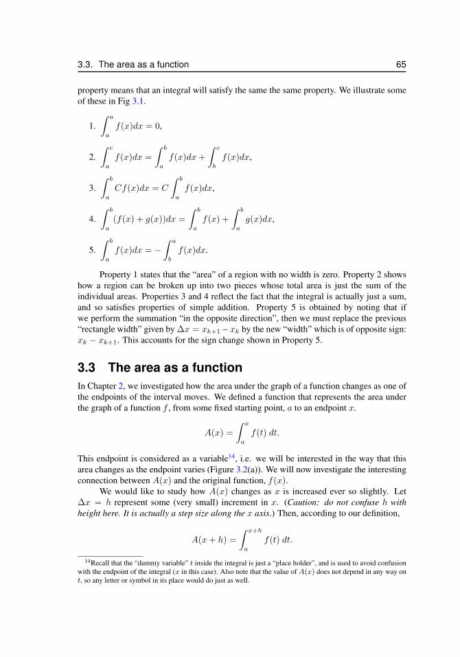
3.3. The area as a function 65
property means that an integral will satisfy the same the same property. We illustrate someof these in Fig 3.1.
1.∫ a
a
f(x)dx = 0,
2.∫ c
a
f(x)dx =
∫ b
a
f(x)dx+
∫ c
b
f(x)dx,
3.∫ b
a
Cf(x)dx = C
∫ b
a
f(x)dx,
4.∫ b
a
(f(x) + g(x))dx =
∫ b
a
f(x) +
∫ b
a
g(x)dx,
5.∫ b
a
f(x)dx = −∫ a
b
f(x)dx.
Property 1 states that the “area” of a region with no width is zero. Property 2 showshow a region can be broken up into two pieces whose total area is just the sum of theindividual areas. Properties 3 and 4 reflect the fact that the integral is actually just a sum,and so satisfies properties of simple addition. Property 5 is obtained by noting that ifwe perform the summation “in the opposite direction”, then we must replace the previous“rectangle width” given by ∆x = xk+1−xk by the new “width” which is of opposite sign:xk − xk+1. This accounts for the sign change shown in Property 5.
3.3 The area as a functionIn Chapter 2, we investigated how the area under the graph of a function changes as one ofthe endpoints of the interval moves. We defined a function that represents the area underthe graph of a function f , from some fixed starting point, a to an endpoint x.
A(x) =
∫ x
a
f(t) dt.
This endpoint is considered as a variable14, i.e. we will be interested in the way that thisarea changes as the endpoint varies (Figure 3.2(a)). We will now investigate the interestingconnection between A(x) and the original function, f(x).
We would like to study how A(x) changes as x is increased ever so slightly. Let∆x = h represent some (very small) increment in x. (Caution: do not confuse h withheight here. It is actually a step size along the x axis.) Then, according to our definition,
A(x+ h) =
∫ x+h
a
f(t) dt.
14Recall that the “dummy variable” t inside the integral is just a “place holder”, and is used to avoid confusionwith the endpoint of the integral (x in this case). Also note that the value of A(x) does not depend in any way ont, so any letter or symbol in its place would do just as well.
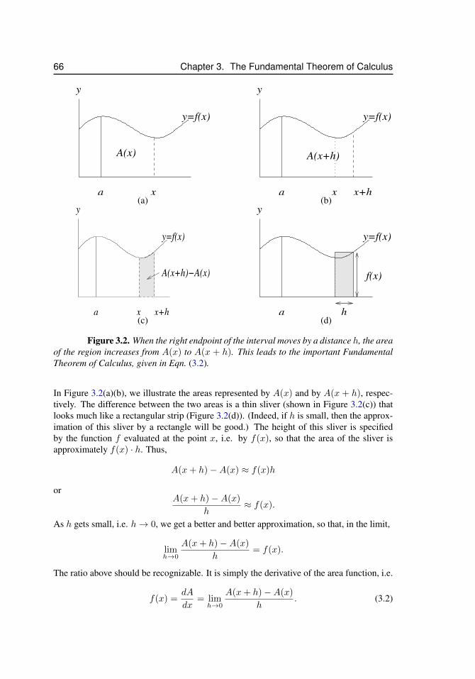
66 Chapter 3. The Fundamental Theorem of Calculus
a x
y
y=f(x)
A(x)
a x
y
y=f(x)
x+h
A(x+h)
(a) (b)
a x
y
y=f(x)
x+h
A(x+h)−A(x)
a
y
y=f(x)
h
f(x)
(c) (d)
Figure 3.2. When the right endpoint of the interval moves by a distance h, the areaof the region increases from A(x) to A(x + h). This leads to the important FundamentalTheorem of Calculus, given in Eqn. (3.2).
In Figure 3.2(a)(b), we illustrate the areas represented by A(x) and by A(x + h), respec-tively. The difference between the two areas is a thin sliver (shown in Figure 3.2(c)) thatlooks much like a rectangular strip (Figure 3.2(d)). (Indeed, if h is small, then the approx-imation of this sliver by a rectangle will be good.) The height of this sliver is specifiedby the function f evaluated at the point x, i.e. by f(x), so that the area of the sliver isapproximately f(x) · h. Thus,
A(x+ h)−A(x) ≈ f(x)h
orA(x+ h)−A(x)
h≈ f(x).
As h gets small, i.e. h→ 0, we get a better and better approximation, so that, in the limit,
limh→0
A(x+ h)−A(x)
h= f(x).
The ratio above should be recognizable. It is simply the derivative of the area function, i.e.
f(x) =dA
dx= limh→0
A(x+ h)−A(x)
h. (3.2)
3.4. The Fundamental Theorem of Calculus 67
We have just given a simple argument in support of an important result, called theFundamental Theorem of Calculus, which is restated below..
3.4 The Fundamental Theorem of Calculus3.4.1 Fundamental theorem of calculus: Part ILet f(x) be a bounded and continuous function on an interval [a, b]. Let
A(x) =
∫ x
a
f(t) dt.
Then for a < x < b,dA
dx= f(x).
In other words, this result says that A(x) is an “antiderivative” (or “anti-derivative”) of theoriginal function, f(x).
Proof
See above argument. and Figure 3.2.
3.4.2 Example: an antiderivativeRecall the connection between functions and their derivatives. Consider the following twofunctions:
g1(x) =x2
2, g2 =
x2
2+ 1.
Clearly, both functions have the same derivative:
g′1(x) = g′2(x) = x.
We would say that x2/2 is an “antiderivative” of x and that (x2/2) + 1 is also an “an-tiderivative” of x. In fact, any function of the form
g(x) =x2
2+ C where C is any constant
is also an “antiderivative” of x.This example illustrates that adding a constant to a given function will not affect
the value of its derivative, or, stated another way, antiderivatives of a given function aredefined only up to some constant. We will use this fact shortly: if A(x) and F (x) are bothantiderivatives of some function f(x), then A(x) = F (x) + C.
3.4.3 Fundamental theorem of calculus: Part IILet f(x) be a continuous function on [a, b]. Suppose F (x) is any antiderivative of f(x).Then for a ≤ x ≤ b,
A(x) =
∫ x
a
f(t) dt = F (x)− F (a).
68 Chapter 3. The Fundamental Theorem of Calculus
Proof
From comments above, we know that a function f(x) could have many different antideriva-tives that differ from one another by some additive constant. We are told that F (x) is anantiderivative of f(x). But from Part I of the Fundamental Theorem, we know that A(x) isalso an antiderivative of f(x). It follows that
A(x) =
∫ x
a
f(t) dt = F (x) + C, where C is some constant. (3.3)
However, by property 1 of definite integrals,
A(a) =
∫ a
a
f(t) = F (a) + C = 0.
Thus,C = −F (a).
Replacing C by −F (a) in equation 3.3 leads to the desired result. Thus
A(x) =
∫ x
a
f(t) dt = F (x)− F (a).
Remark 1: Implications
This theorem has tremendous implications, because it allows us to use a powerful newtool in determining areas under curves. Instead of the drudgery of summations in order tocompute areas, we will be able to use a shortcut: find an antiderivative, evaluate it at thetwo endpoints a, b of the interval of interest, and subtract the results to get the area. In thecase of elementary functions, this will be very easy and convenient.
Remark 2: Notation
We will often use the notation
F (t)|xa = F (x)− F (a)
to denote the difference in the values of a function at two endpoints.
3.5 Review of derivatives (and antiderivatives)By remarks above, we see that integration is related to “anti-differentiation”. This moti-vates a review of derivatives of common functions. Table 3.1 lists functions f(x) and theirderivatives f ′(x) (in the first two columns) and functions f(x) and their antiderivativesF (x) in the subsequent two columns. These will prove very helpful in our calculations ofbasic integrals.
As an example, consider the polynomial
p(x) = a0 + a1x+ a2x2 + a3x
3 + . . .
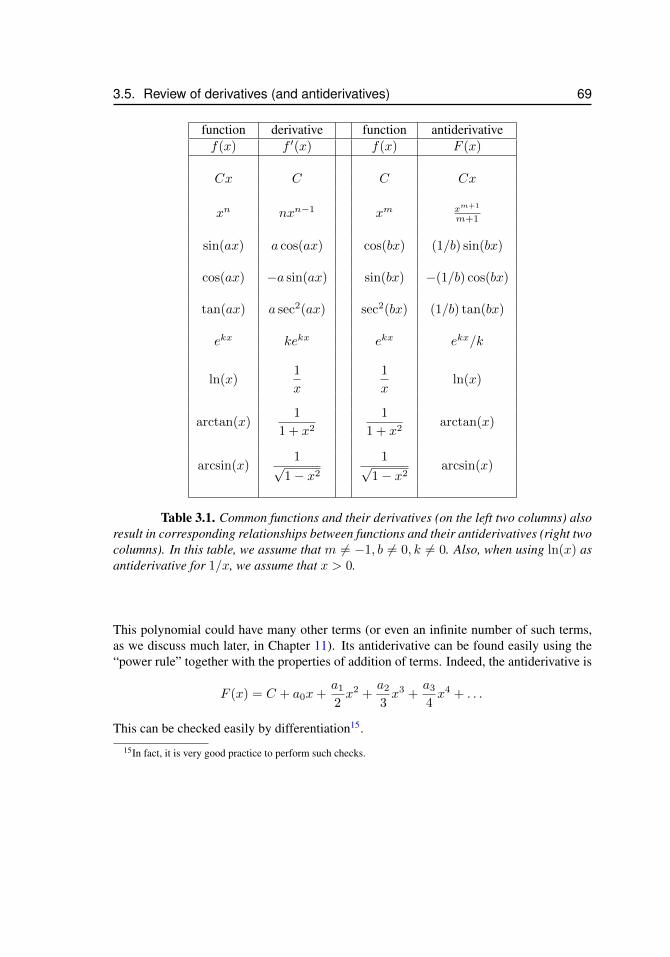
3.5. Review of derivatives (and antiderivatives) 69
function derivative function antiderivativef(x) f ′(x) f(x) F (x)
Cx C C Cx
xn nxn−1 xm xm+1
m+1
sin(ax) a cos(ax) cos(bx) (1/b) sin(bx)
cos(ax) −a sin(ax) sin(bx) −(1/b) cos(bx)
tan(ax) a sec2(ax) sec2(bx) (1/b) tan(bx)
ekx kekx ekx ekx/k
ln(x)1
x
1
xln(x)
arctan(x)1
1 + x2
1
1 + x2arctan(x)
arcsin(x)1√
1− x2
1√1− x2
arcsin(x)
Table 3.1. Common functions and their derivatives (on the left two columns) alsoresult in corresponding relationships between functions and their antiderivatives (right twocolumns). In this table, we assume that m 6= −1, b 6= 0, k 6= 0. Also, when using ln(x) asantiderivative for 1/x, we assume that x > 0.
This polynomial could have many other terms (or even an infinite number of such terms,as we discuss much later, in Chapter 11). Its antiderivative can be found easily using the“power rule” together with the properties of addition of terms. Indeed, the antiderivative is
F (x) = C + a0x+a1
2x2 +
a2
3x3 +
a3
4x4 + . . .
This can be checked easily by differentiation15.
15In fact, it is very good practice to perform such checks.
70 Chapter 3. The Fundamental Theorem of Calculus
3.6 Examples: Computing areas with theFundamental Theorem of Calculus
3.6.1 Example 1: The area under a polynomialConsider the polynomial
p(x) = 1 + x+ x2 + x3.
(Here we have taken the first few terms from the example of the last section with coeffi-cients all set to 1.) Then, computing
I =
∫ 1
0
p(x) dx
leads to
I =
∫ 1
0
(1 + x+ x2 + x3) dx = (x+1
2x2 +
1
3x3 +
1
4x4)
∣∣∣∣10
= 1 +1
2+
1
3+
1
4≈ 2.083.
3.6.2 Example 2: Simple areasDetermine the values of the following definite integrals by finding antiderivatives and usingthe Fundamental Theorem of Calculus:
1. I =
∫ 1
0
x2 dx,
2. I =
∫ 1
−1
(1− x2) dx,
3. I =
∫ 1
−1
e−2x dx,
4. I =
∫ 2π
−2π
sin(x
2
)dx,
Solutions
1. An antiderivative of f(x) = x2 is F (x) = (x3/3), thus
I =
∫ 1
0
x2dx = F (x)
∣∣∣∣10
= (1/3)(x3)
∣∣∣∣10
=1
3(13 − 0) =
1
3.
2. An antiderivative of f(x) = (1− x2) is F (x) = x− (x3/3), thus
I =
∫ 1
−1
(1− x2) dx = F (x)
∣∣∣∣1−1
=
(x− x3
3
) ∣∣∣∣1−1
=
(1− 13
3
)−(
(−1)− (−1)3
3
)= 4/3
See comment 1 below for a simpler way to compute this integral.

3.6. Examples: Computing areas with the Fundamental Theorem of Calculus 71
2
−1 0 1x
y=1−x
Figure 3.3. We can exploit the symmetry of the function f(x) = 1 − x2 in thesecond integral of Examples 3.6.2. We can integrate over 0 ≤ x ≤ 1 and double the result.
3. An antiderivative of e−2x is F (x) = (−1/2)e−2x. Thus,
I =
∫ 1
−1
e−2x dx = F (x)
∣∣∣∣1−1
= (−1/2)(e−2x)
∣∣∣∣1−1
= (−1/2)(e−2 − e2).
4. An antiderivative of sin(x/a) is F (x) = − cos(x/a)/(1/a) = −a cos(x/a). Thus
I =
∫ 2π
−2π
sin(x
2
)dx = −2 cos
(x2
) ∣∣∣∣2π−2π
= −2 (cos (π)− cos (−π))
= −2(−1− (−1)) = 0.
See comment 2 below for a simpler way to compute this integral.
Comment 1: The evaluation of Integral 2 in the examples above is tricky only in thatsigns can easily get garbled when we plug in the endpoint at -1. However, we can simplifyour work by noting the symmetry of the function f(x) = 1− x2 on the given interval. Asshown in Fig 3.3, the areas to the right and to the left of x = 0 are the same for the interval−1 ≤ x ≤ 1. This stems directly from the fact that the function considered is even16.Thus, we can immediately write
I =
∫ 1
−1
(1− x2) dx = 2
∫ 1
0
(1− x2) dx = 2
(x− x3
3
) ∣∣∣∣10
= 2
(1− 13
3
)= 4/3.
Note that this calculation is simpler since the endpoint at x = 0 is trivial to plug in.We state the general result we have obtained, which holds true for any function with
even symmetry integrated on a symmetric interval about x = 0:
If f(x) is an even function, then∫ a
−af(x) dx = 2
∫ a
0
f(x) dx. (3.4)
16Recall that a function f(x) is even if f(x) = f(−x) for all x. A function is odd if f(x) = −f(−x).
72 Chapter 3. The Fundamental Theorem of Calculus
Caution: The function f(x) must be integrable, i.e. f(x) must exist and be definedover the entire interval x ∈ [−a, a]. For example, the integrand in
∫ 2
−2x−2dx is even but
requires more careful considerations because it does not exist at x = 0 (see Chapter 7).
Similarly, if f(x) is an odd function then the symmetry yields an even simpler resulton a symmetric interval about x = 0:
If f(x) is an odd function, then∫ a
−af(x) dx = 0 for any a. (3.5)
Caution: Again, f(x) must be integrable over the entire interval x ∈ [−a, a]. For ex-ample, even though the integrand in
∫ 2
−21x dx is odd, the integral requires more careful
considerations because the integrand does not exist at x = 0 (see Chapter 7).
Comment 2: We can exploit symmetries for a simpler evaluation of Integral 4 above:by realizing that sin(x2 ) is an odd function and also noticing that the integration boundsare symmetric about x = 0, we immediately conclude that the integral evaluates to zerowithout requiring any actual calculations.
3.6.3 Example 3: The area between two curvesThe definite integral is an area of a somewhat special type of region, i.e., an axis, twovertical lines (x = a and x = b) and the graph of a function. However, using additive(or subtractive) properties of areas, we can generalize to computing areas of other regions,including those bounded by the graphs of two functions.
(a) Find the area enclosed between the graphs of the functions y = x3 and y = x1/3 in thefirst quadrant.
(b) Find the area enclosed between the graphs of the functions y = x3 and y = x in thefirst quadrant.
(c) What is the relationship of these two areas? What is the relationship of the functionsy = x3 and y = x1/3 that leads to this relationship between the two areas?
Solution
(a) The two curves, y = x3 and y = x1/3, intersect at x = 0 and at x = 1 in the firstquadrant. Thus the interval that we will be concerned with is 0 < x < 1. On thisinterval, x1/3 > x3, so that the area we want to find can be expressed as:
A1 =
∫ 1
0
(x1/3 − x3
)dx.
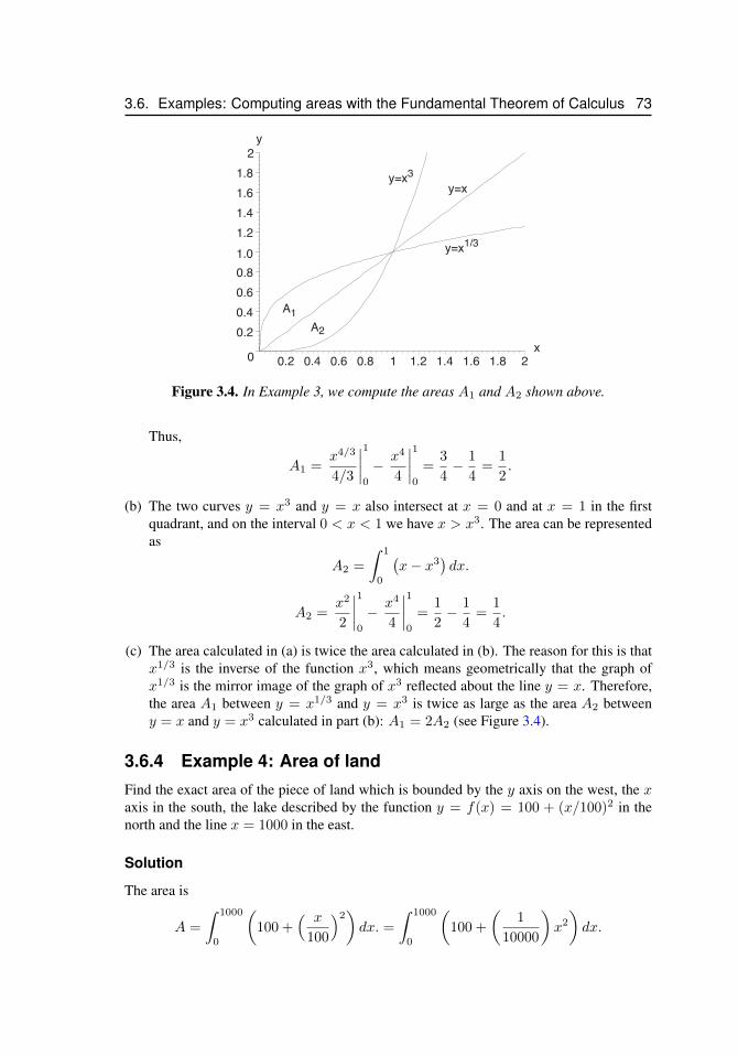
3.6. Examples: Computing areas with the Fundamental Theorem of Calculus 73
A
A
y=x
y=x
y=x
0
0.2
0.4
0.6
0.8
1.0
1.2
1.4
1.6
1.8
2y
0.2 0.4 0.6 0.8 1 1.2 1.4 1.6 1.8 2x
1
2
3
1/3
Figure 3.4. In Example 3, we compute the areas A1 and A2 shown above.
Thus,
A1 =x4/3
4/3
∣∣∣∣10
− x4
4
∣∣∣∣10
=3
4− 1
4=
1
2.
(b) The two curves y = x3 and y = x also intersect at x = 0 and at x = 1 in the firstquadrant, and on the interval 0 < x < 1 we have x > x3. The area can be representedas
A2 =
∫ 1
0
(x− x3
)dx.
A2 =x2
2
∣∣∣∣10
− x4
4
∣∣∣∣10
=1
2− 1
4=
1
4.
(c) The area calculated in (a) is twice the area calculated in (b). The reason for this is thatx1/3 is the inverse of the function x3, which means geometrically that the graph ofx1/3 is the mirror image of the graph of x3 reflected about the line y = x. Therefore,the area A1 between y = x1/3 and y = x3 is twice as large as the area A2 betweeny = x and y = x3 calculated in part (b): A1 = 2A2 (see Figure 3.4).
3.6.4 Example 4: Area of landFind the exact area of the piece of land which is bounded by the y axis on the west, the xaxis in the south, the lake described by the function y = f(x) = 100 + (x/100)2 in thenorth and the line x = 1000 in the east.
Solution
The area is
A =
∫ 1000
0
(100 +
( x
100
)2)dx. =
∫ 1000
0
(100 +
(1
10000
)x2
)dx.
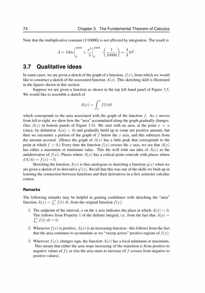
74 Chapter 3. The Fundamental Theorem of Calculus
Note that the multiplicative constant (1/10000) is not affected by integration. The result is
A = 100x
∣∣∣∣1000
0
+x3
3
∣∣∣∣1000
0
·(
1
10000
)=
4
3105.
3.7 Qualitative ideasIn some cases, we are given a sketch of the graph of a function, f(x), from which we wouldlike to construct a sketch of the associated function A(x). This sketching skill is illustratedin the figures shown in this section.
Suppose we are given a function as shown in the top left hand panel of Figure 3.5.We would like to assemble a sketch of
A(x) =
∫ x
a
f(t)dt
which corresponds to the area associated with the graph of the function f . As x movesfrom left to right, we show how the “area” accumulated along the graph gradually changes.(See A(x) in bottom panels of Figure 3.5): We start with no area, at the point x = a(since, by definition A(a) = 0) and gradually build up to some net positive amount, butthen we encounter a portion of the graph of f below the x axis, and this subtracts fromthe amount accrued. (Hence the graph of A(x) has a little peak that corresponds to thepoint at which f = 0.) Every time the function f(x) crosses the x axis, we see that A(x)has either a maximum or minimum value. This fits well with our idea of A(x) as theantiderivative of f(x): Places where A(x) has a critical point coincide with places wheredA/dx = f(x) = 0.
Sketching the function A(x) is thus analogous to sketching a function g(x) when weare given a sketch of its derivative g′(x). Recall that this was one of the skills we built up inlearning the connection between functions and their derivatives in a first semester calculuscourse.
Remarks
The following remarks may be helpful in gaining confidence with sketching the “area”function A(x) =
∫ xaf(t) dt, from the original function f(x):
1. The endpoint of the interval, a on the x axis indicates the place at which A(x) = 0.This follows from Property 1 of the definite integral, i.e. from the fact that A(a) =∫ aaf(t) dt = 0.
2. Whenever f(x) is positive,A(x) is an increasing function - this follows from the factthat the area continues to accumulate as we “sweep across” positive regions of f(x).
3. Wherever f(x), changes sign, the function A(x) has a local minimum or maximum.This means that either the area stops increasing (if the transition is from positive to
negative values of f ), or else the area starts to increase (if f crosses from negative topositive values).
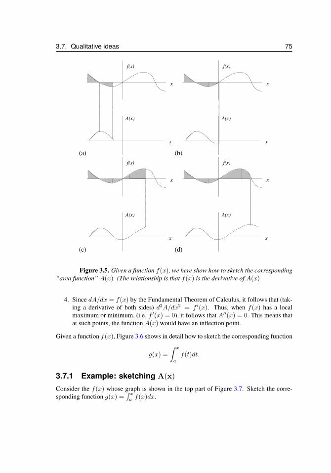
3.7. Qualitative ideas 75
(a)
x
f(x)
x
A(x)
(b)
x
f(x)
x
A(x)
(c)
x
f(x)
x
A(x)
(d)
x
f(x)
x
A(x)
Figure 3.5. Given a function f(x), we here show how to sketch the corresponding“area function” A(x). (The relationship is that f(x) is the derivative of A(x)
4. Since dA/dx = f(x) by the Fundamental Theorem of Calculus, it follows that (tak-ing a derivative of both sides) d2A/dx2 = f ′(x). Thus, when f(x) has a localmaximum or minimum, (i.e. f ′(x) = 0), it follows that A′′(x) = 0. This means thatat such points, the function A(x) would have an inflection point.
Given a function f(x), Figure 3.6 shows in detail how to sketch the corresponding function
g(x) =
∫ x
a
f(t)dt.
3.7.1 Example: sketching A(x)
Consider the f(x) whose graph is shown in the top part of Figure 3.7. Sketch the corre-sponding function g(x) =
∫ xaf(x)dx.
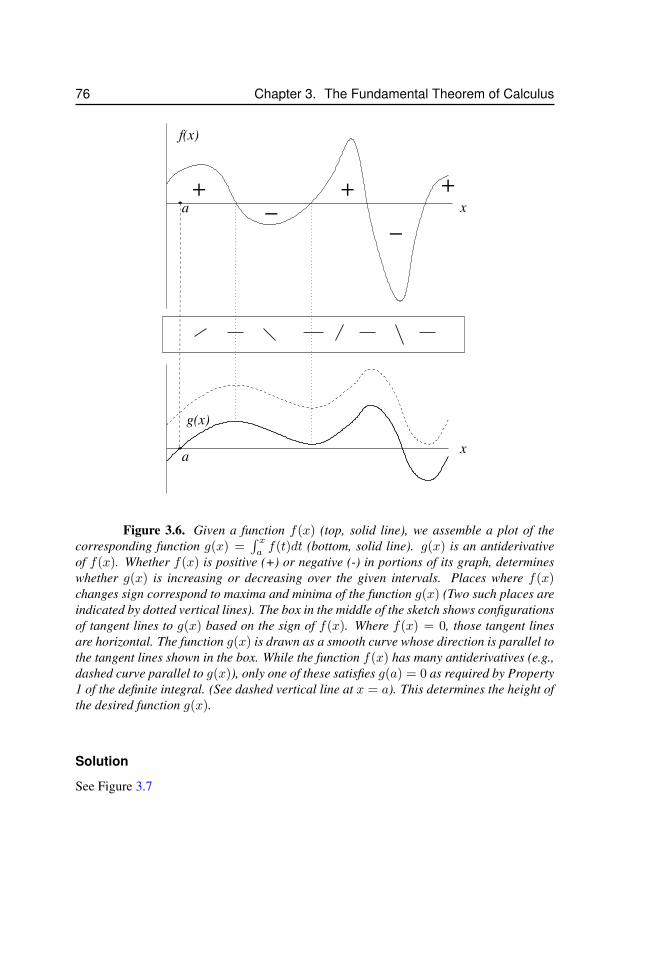
76 Chapter 3. The Fundamental Theorem of Calculus
a
x
x
f(x)
g(x)
+−
+
−
+a
Figure 3.6. Given a function f(x) (top, solid line), we assemble a plot of thecorresponding function g(x) =
∫ xaf(t)dt (bottom, solid line). g(x) is an antiderivative
of f(x). Whether f(x) is positive (+) or negative (-) in portions of its graph, determineswhether g(x) is increasing or decreasing over the given intervals. Places where f(x)changes sign correspond to maxima and minima of the function g(x) (Two such places areindicated by dotted vertical lines). The box in the middle of the sketch shows configurationsof tangent lines to g(x) based on the sign of f(x). Where f(x) = 0, those tangent linesare horizontal. The function g(x) is drawn as a smooth curve whose direction is parallel tothe tangent lines shown in the box. While the function f(x) has many antiderivatives (e.g.,dashed curve parallel to g(x)), only one of these satisfies g(a) = 0 as required by Property1 of the definite integral. (See dashed vertical line at x = a). This determines the height ofthe desired function g(x).
Solution
See Figure 3.7
3.8. Prelude to improper integrals 77
x
+
−
+
f(x)
g(x)
a
a
x
Figure 3.7. The original functions, f(x) is shown above. The correspondingfunctions g(x) is drawn below.
3.8 Prelude to improper integralsThe Fundamental Theorem has a number of restrictions that must be satisfied before itsresults can be applied. In this section we look at some examples in which care must beused. The examples of this section should be compared with our chapter on ImproperIntegrals. In particular one must be careful in applying the Fundamental theorem when theintegrand has a discontinuity within the region of integration.
3.8.1 Function unbounded IConsider the definite integral ∫ 2
0
1
xdx.
The function f(x) = 1x is discontinuous at x = 0, and unbounded on any interval that
contains the point x = 0, i.e. limx→0±1x = ±∞. Hence we cannot directly evaluate this
integral using the Fundamental theorem. However we can show that limε→0+
∫ 2
ε1x dx =
∞. Indeed the integrand is continuous on the interval (ε, 2) for all ε > 0. The Fundamentaltheorem therefore tells us ∫ 2
ε
1
xdx = log(2)− log(ε).
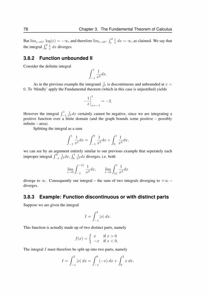
78 Chapter 3. The Fundamental Theorem of Calculus
But limε→0+ log(ε) = −∞, and therefore limε→0+
∫ 2
ε1x dx =∞, as claimed. We say that
the integral∫ 2
01x dx diverges.
3.8.2 Function unbounded IIConsider the definite integral ∫ 1
−1
1
x2dx.
As in the previous example the integrand 1x2 is discontinuous and unbounded at x =
0. To ‘blindly’ apply the Fundamental theorem (which in this case is unjustified) yields
− 1
x
∣∣∣∣1x=−1
= −2.
However the integral∫ 1
−11x2 dx certainly cannot be negative, since we are integrating a
positive function over a finite domain (and the graph bounds some positive – possiblyinfinite – area).
Splitting the integral as a sum∫ 1
−1
1
x2dx =
∫ 0
−1
1
x2dx+
∫ 1
0
1
x2dx,
we can see by an argument entirely similar to our previous example that seperately eachimproper integral
∫ 0
−11x2 dx,
∫ 1
01x2 dx diverges, i.e. both
limε→0
∫ −|ε|−1
1
x2dx, lim
ε→0
∫ 1
|ε|
1
x2dx
diverge to ∞. Consequently our integral – the sum of two integrals diverging to +∞ –diverges.
3.8.3 Example: Function discontinuous or with distinct partsSuppose we are given the integral
I =
∫ 2
−1
|x| dx.
This function is actually made up of two distinct parts, namely
f(x) =
{x if x > 0−x if x < 0.
The integral I must therefore be split up into two parts, namely
I =
∫ 2
−1
|x| dx =
∫ 0
−1
(−x) dx+
∫ 2
0
x dx.
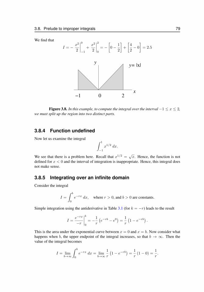
3.8. Prelude to improper integrals 79
We find that
I = − x2
2
∣∣∣∣0−1
+x2
2
∣∣∣∣20
= −[0− 1
2
]+
[4
2− 0
]= 2.5
x
yy= |x|
−1 20
Figure 3.8. In this example, to compute the integral over the interval−1 ≤ x ≤ 2,we must split up the region into two distinct parts.
3.8.4 Function undefinedNow let us examine the integral ∫ 1
−1
x1/2 dx.
We see that there is a problem here. Recall that x1/2 =√x. Hence, the function is not
defined for x < 0 and the interval of integration is inappropriate. Hence, this integral doesnot make sense.
3.8.5 Integrating over an infinite domainConsider the integral
I =
∫ b
0
e−rx dx, where r > 0, and b > 0 are constants.
Simple integration using the antiderivative in Table 3.1 (for k = −r) leads to the result
I =e−rx
−r
∣∣∣∣b0
= −1
r
(e−rb − e0
)=
1
r
(1− e−rb
).
This is the area under the exponential curve between x = 0 and x = b. Now consider whathappens when b, the upper endpoint of the integral increases, so that b → ∞. Then thevalue of the integral becomes
I = limb→∞
∫ b
0
e−rx dx = limb→∞
1
r
(1− e−rb
)=
1
r(1− 0) =
1
r.
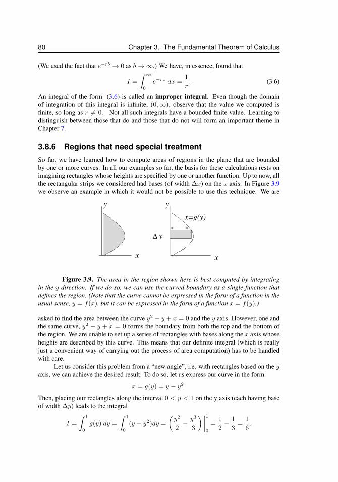
80 Chapter 3. The Fundamental Theorem of Calculus
(We used the fact that e−rb → 0 as b→∞.) We have, in essence, found that
I =
∫ ∞0
e−rx dx =1
r. (3.6)
An integral of the form (3.6) is called an improper integral. Even though the domainof integration of this integral is infinite, (0,∞), observe that the value we computed isfinite, so long as r 6= 0. Not all such integrals have a bounded finite value. Learning todistinguish between those that do and those that do not will form an important theme inChapter 7.
3.8.6 Regions that need special treatmentSo far, we have learned how to compute areas of regions in the plane that are boundedby one or more curves. In all our examples so far, the basis for these calculations rests onimagining rectangles whose heights are specified by one or another function. Up to now, allthe rectangular strips we considered had bases (of width ∆x) on the x axis. In Figure 3.9we observe an example in which it would not be possible to use this technique. We are
∆ y
x=g(y)
x
yy
x
Figure 3.9. The area in the region shown here is best computed by integratingin the y direction. If we do so, we can use the curved boundary as a single function thatdefines the region. (Note that the curve cannot be expressed in the form of a function in theusual sense, y = f(x), but it can be expressed in the form of a function x = f(y).)
asked to find the area between the curve y2 − y + x = 0 and the y axis. However, one andthe same curve, y2 − y + x = 0 forms the boundary from both the top and the bottom ofthe region. We are unable to set up a series of rectangles with bases along the x axis whoseheights are described by this curve. This means that our definite integral (which is reallyjust a convenient way of carrying out the process of area computation) has to be handledwith care.
Let us consider this problem from a “new angle”, i.e. with rectangles based on the yaxis, we can achieve the desired result. To do so, let us express our curve in the form
x = g(y) = y − y2.
Then, placing our rectangles along the interval 0 < y < 1 on the y axis (each having baseof width ∆y) leads to the integral
I =
∫ 1
0
g(y) dy =
∫ 1
0
(y − y2)dy =
(y2
2− y3
3
) ∣∣∣∣10
=1
2− 1
3=
1
6.
3.9. Summary 81
3.9 SummaryIn this chapter we first recapped the definition of the definite integral in Section 3.1, recalledits connection to an area in the plane under the graph of some function f(x), and examinedits basic properties.
If one of the endpoints, x of the integral is allowed to vary, the area it represents,A(x), becomes a function of x. Our construction in Figure 3.2 showed that there is a con-nection between the derivative A′(x) of the area and the function f(x). Indeed, we showedthat A′(x) = f(x) and argued that this makes A(x) an antiderivative of the function f(x).
This important connection between integrals and antiderivatives is the crux of In-tegral Calculus, forming the Fundamental Theorem of Calculus. Its significance is thatfinding areas need not be as tedious and labored as the calculation of Riemann sums thatformed the bulk of Chapter 2. Rather, we can take a shortcut using antidifferentiation.
Motivated by this very important result, we reviewed some common functions andderivatives, and used this to relate functions and their antiderivatives in Table 3.1. Weused these antiderivatives to calculate areas in several examples. Finally, we extended thetreatment to include qualitative sketches of functions and their antiderivatives.
As we will see in upcoming chapters, the ideas presented here have a much widerrange of applicability than simple area calculations. Indeed, we will shortly show that thesame concepts can be used to calculate net changes in continually varying processes, tocompute volumes of various shapes, to determine displacement from velocity, mass fromdensities, as well as a host of other quantities that involve a process of accumulation. Theseideas will be investigated in Chapters 4, and 5.
82 Chapter 3. The Fundamental Theorem of Calculus
3.10 ExercisesExercise 3.1
(a) Give a concise statement of the Fundamental Theorem of Calculus.
(b) Why is it a useful practical tool?
Exercise 3.2 Consider the function y = f(x) = ex on the interval [0, 1].Find the area under the graph of this function over this interval using the Fundamental
Theorem of Calculus.
Exercise 3.3 Determine the values of the integrals shown below, using the FundamentalTheorem of Calculus (i.e. find the anti-derivative of each of the functions and evaluate atthe two endpoints.)
(a)∫ 1
0
2xdx
(b)∫ 1
-1(1− x)dx
Exercise 3.4 Use the Fundamental Theorem of Calculus to compute each of the followingintegrals. The last few are a little more challenging, and will require special care. Some ofthese integrals may not exist. Explain why.
(a)∫ π
0
sin(x) dx (b)∫ π
4
0
2 sin(x) dx (c)∫ π
2
0
cos(x) dx
(d)∫ π
4
−π42 cos(x) dx (e)
∫ 3
2
(x− 2) dx (f)∫ 1
−1
(x− 1) dx
(g)∫ 1
−1
(x2 + 1) dx (h)∫ 4
0
(x+ 1)2 dx (i)∫ 4
0
x1/2 dx
(j)∫ 1
0
3x1/2 dx (k)∫ 4
1
(1 +√x) dx (l)
∫ 2
1
3
xdx
(m)∫ 3
1
2
xdx (n)
∫ 1
0
2ex dx (o)∫ −3
−2
x1/3 dx
(p)∫ 0
−1
x1/2 dx (q)∫ 1
−1
x−2 dx (r)∫ 1
−1
2|x| dx
(s)∫ 2
0
1
xdx (t)
∫ 1
−1
2
x
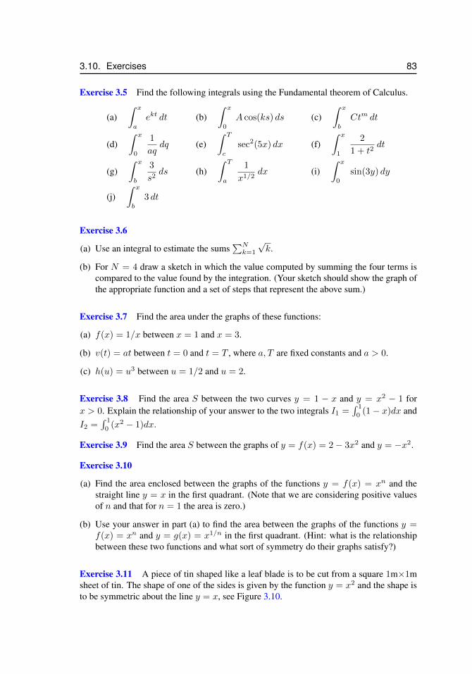
3.10. Exercises 83
Exercise 3.5 Find the following integrals using the Fundamental theorem of Calculus.
(a)∫ x
a
ekt dt (b)∫ x
0
A cos(ks) ds (c)∫ x
b
Ctm dt
(d)∫ x
0
1
aqdq (e)
∫ T
c
sec2(5x) dx (f)∫ x
1
2
1 + t2dt
(g)∫ x
b
3
s2ds (h)
∫ T
a
1
x1/2dx (i)
∫ x
0
sin(3y) dy
(j)∫ x
b
3 dt
Exercise 3.6
(a) Use an integral to estimate the sums∑Nk=1
√k.
(b) For N = 4 draw a sketch in which the value computed by summing the four terms iscompared to the value found by the integration. (Your sketch should show the graph ofthe appropriate function and a set of steps that represent the above sum.)
Exercise 3.7 Find the area under the graphs of these functions:
(a) f(x) = 1/x between x = 1 and x = 3.
(b) v(t) = at between t = 0 and t = T , where a, T are fixed constants and a > 0.
(c) h(u) = u3 between u = 1/2 and u = 2.
Exercise 3.8 Find the area S between the two curves y = 1 − x and y = x2 − 1 forx > 0. Explain the relationship of your answer to the two integrals I1 =
∫ 1
0(1− x)dx and
I2 =∫ 1
0(x2 − 1)dx.
Exercise 3.9 Find the area S between the graphs of y = f(x) = 2− 3x2 and y = −x2.
Exercise 3.10
(a) Find the area enclosed between the graphs of the functions y = f(x) = xn and thestraight line y = x in the first quadrant. (Note that we are considering positive valuesof n and that for n = 1 the area is zero.)
(b) Use your answer in part (a) to find the area between the graphs of the functions y =f(x) = xn and y = g(x) = x1/n in the first quadrant. (Hint: what is the relationshipbetween these two functions and what sort of symmetry do their graphs satisfy?)
Exercise 3.11 A piece of tin shaped like a leaf blade is to be cut from a square 1m×1msheet of tin. The shape of one of the sides is given by the function y = x2 and the shape isto be symmetric about the line y = x, see Figure 3.10.
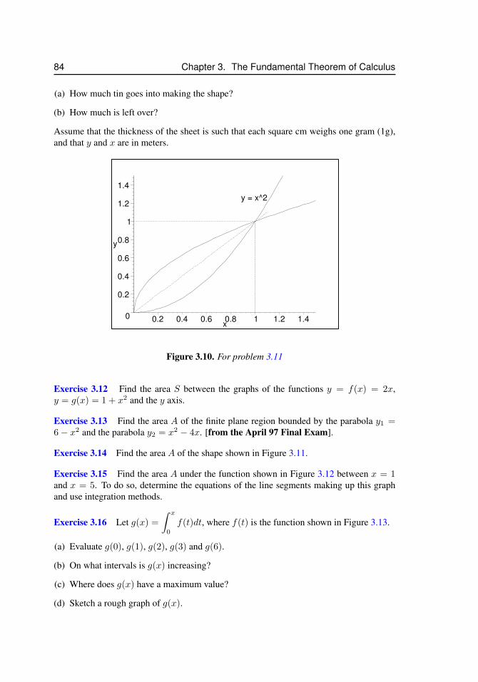
84 Chapter 3. The Fundamental Theorem of Calculus
(a) How much tin goes into making the shape?
(b) How much is left over?
Assume that the thickness of the sheet is such that each square cm weighs one gram (1g),and that y and x are in meters.
y = x^2
0
0.2
0.4
0.6
0.8
1
1.2
1.4
y
0.2 0.4 0.6 0.8 1 1.2 1.4x
Figure 3.10. For problem 3.11
Exercise 3.12 Find the area S between the graphs of the functions y = f(x) = 2x,y = g(x) = 1 + x2 and the y axis.
Exercise 3.13 Find the area A of the finite plane region bounded by the parabola y1 =6− x2 and the parabola y2 = x2 − 4x. [from the April 97 Final Exam].
Exercise 3.14 Find the area A of the shape shown in Figure 3.11.
Exercise 3.15 Find the area A under the function shown in Figure 3.12 between x = 1and x = 5. To do so, determine the equations of the line segments making up this graphand use integration methods.
Exercise 3.16 Let g(x) =
∫ x
0
f(t)dt, where f(t) is the function shown in Figure 3.13.
(a) Evaluate g(0), g(1), g(2), g(3) and g(6).
(b) On what intervals is g(x) increasing?
(c) Where does g(x) have a maximum value?
(d) Sketch a rough graph of g(x).
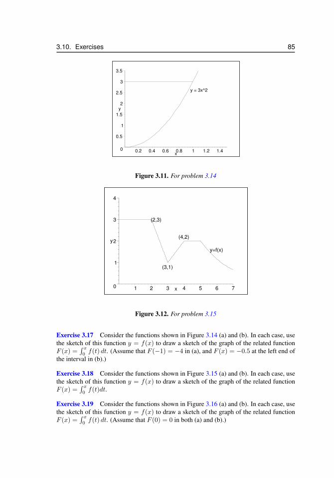
3.10. Exercises 85
y = 3x^2
0
0.5
1
1.5
2
2.5
3
3.5
y
0.2 0.4 0.6 0.8 1 1.2 1.4x
Figure 3.11. For problem 3.14
(2,3)
(4,2)
y=f(x)
(3,1)
0
1
2
3
4
y
1 2 3 4 5 6 7x
Figure 3.12. For problem 3.15
Exercise 3.17 Consider the functions shown in Figure 3.14 (a) and (b). In each case, usethe sketch of this function y = f(x) to draw a sketch of the graph of the related functionF (x) =
∫ x0f(t) dt. (Assume that F (−1) = −4 in (a), and F (x) = −0.5 at the left end of
the interval in (b).)
Exercise 3.18 Consider the functions shown in Figure 3.15 (a) and (b). In each case, usethe sketch of this function y = f(x) to draw a sketch of the graph of the related functionF (x) =
∫ x0f(t)dt.
Exercise 3.19 Consider the functions shown in Figure 3.16 (a) and (b). In each case, usethe sketch of this function y = f(x) to draw a sketch of the graph of the related functionF (x) =
∫ x0f(t) dt. (Assume that F (0) = 0 in both (a) and (b).)
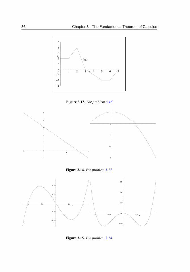
86 Chapter 3. The Fundamental Theorem of Calculus
f (x)
–3
–2
–1
0
1
2
3
4
5
y
1 2 3 4 5 6 7x
Figure 3.13. For problem 3.16
–1
0
1
2
3
4
5
–1 1 2x
–3
–2
–1
0
1
x
Figure 3.14. For problem 3.17
–0.4
–0.2
0.2
0.4
–1 –0.5 0.5 1x
–0.2
0
0.2
0.4
0.6
–1 –0.5 0.5 1x
Figure 3.15. For problem 3.18
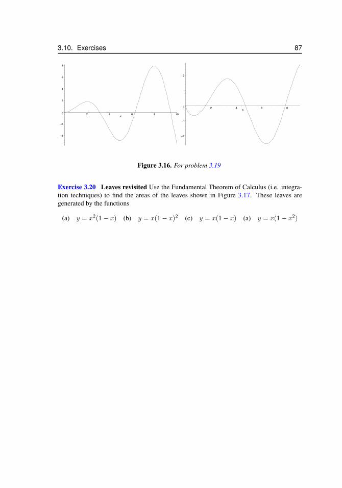
3.10. Exercises 87
–4
–2
0
2
4
6
8
2 4 6 8 10x
–2
–1
0
1
2
2 4 6 8x
Figure 3.16. For problem 3.19
Exercise 3.20 Leaves revisited Use the Fundamental Theorem of Calculus (i.e. integra-tion techniques) to find the areas of the leaves shown in Figure 3.17. These leaves aregenerated by the functions
(a) y = x2(1− x) (b) y = x(1− x)2 (c) y = x(1− x) (a) y = x(1− x2)
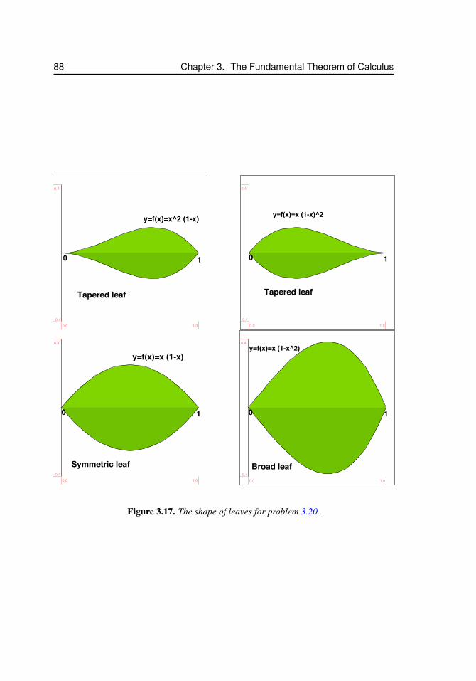
88 Chapter 3. The Fundamental Theorem of Calculus
Tapered leaf
y=f(x)=x^2 (1-x)
0 1
0.0 1.0-0.4
0.4
Tapered leaf
y=f(x)=x (1-x)^2
10
0.0 1.0-0.4
0.4
Symmetric leaf
y=f(x)=x (1-x)
10
0.0 1.0-0.4
0.4
Broad leaf
y=f(x)=x (1-x^2)
10
0.0 1.0-0.4
0.4
Figure 3.17. The shape of leaves for problem 3.20.
Chapter 4
Applications of thedefinite integral tovelocities and rates
4.1 IntroductionIn this chapter, we encounter a number of applications of the definite integral to practicalproblems. We will discuss the connection between acceleration, velocity and displacementof a moving object, a topic we visited in an earlier, Differential Calculus Course. Herewe will show that the notion of antiderivatives and integrals allows us to deduce details ofthe motion of an object from underlying Laws of Motion. We will consider both uniformand accelerated motion, and recall how air resistance can be described, and what effect itinduces.
An important connection is made in this chapter between a rate of change (e.g. rateof growth) and the total change (i.e. the net change resulting from all the accumulation andloss over a time span). We show that such examples also involve the concept of integration,which, fundamentally, is a cumulative summation of infinitesimal changes. This allows usto extend the utility of the mathematical tools to a variety of novel situations. We will seeexamples of this type in Sections 4.3 and 4.4.
Several other important ideas are introduced in this chapter. We encounter for thefirst time the idea of spatial density, and see that integration can also be used to “add up”the total amount of material distributed over space. In Section 5.2.2, this idea is applied tothe density of cars along a highway. We also consider mass distributions and the notion ofa center of mass.
Finally, we also show that the definite integral is useful for determining the averagevalue of a function, as discussed in Section 4.5. In all these examples, the important stepis to properly set up the definite integral that corresponds to the desired net change. Com-putations at this stage are relatively straightforward to emphasize the process of setting upthe appropriate integrals and understanding what they represent.
89
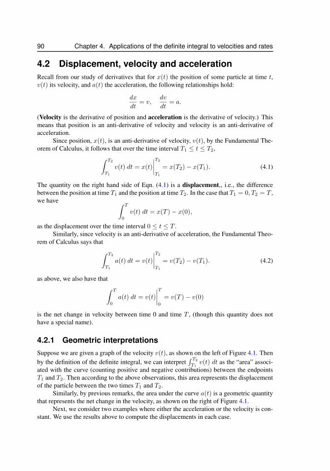
90 Chapter 4. Applications of the definite integral to velocities and rates
4.2 Displacement, velocity and accelerationRecall from our study of derivatives that for x(t) the position of some particle at time t,v(t) its velocity, and a(t) the acceleration, the following relationships hold:
dx
dt= v,
dv
dt= a.
(Velocity is the derivative of position and acceleration is the derivative of velocity.) Thismeans that position is an anti-derivative of velocity and velocity is an anti-derivative ofacceleration.
Since position, x(t), is an anti-derivative of velocity, v(t), by the Fundamental The-orem of Calculus, it follows that over the time interval T1 ≤ t ≤ T2,∫ T2
T1
v(t) dt = x(t)
∣∣∣∣T2
T1
= x(T2)− x(T1). (4.1)
The quantity on the right hand side of Eqn. (4.1) is a displacement,, i.e., the differencebetween the position at time T1 and the position at time T2. In the case that T1 = 0, T2 = T ,we have ∫ T
0
v(t) dt = x(T )− x(0),
as the displacement over the time interval 0 ≤ t ≤ T .Similarly, since velocity is an anti-derivative of acceleration, the Fundamental Theo-
rem of Calculus says that∫ T2
T1
a(t) dt = v(t)
∣∣∣∣T2
T1
= v(T2)− v(T1). (4.2)
as above, we also have that∫ T
0
a(t) dt = v(t)
∣∣∣∣T0
= v(T )− v(0)
is the net change in velocity between time 0 and time T , (though this quantity does nothave a special name).
4.2.1 Geometric interpretationsSuppose we are given a graph of the velocity v(t), as shown on the left of Figure 4.1. Thenby the definition of the definite integral, we can interpret
∫ T2
T1v(t) dt as the “area” associ-
ated with the curve (counting positive and negative contributions) between the endpointsT1 and T2. Then according to the above observations, this area represents the displacementof the particle between the two times T1 and T2.
Similarly, by previous remarks, the area under the curve a(t) is a geometric quantitythat represents the net change in the velocity, as shown on the right of Figure 4.1.
Next, we consider two examples where either the acceleration or the velocity is con-stant. We use the results above to compute the displacements in each case.
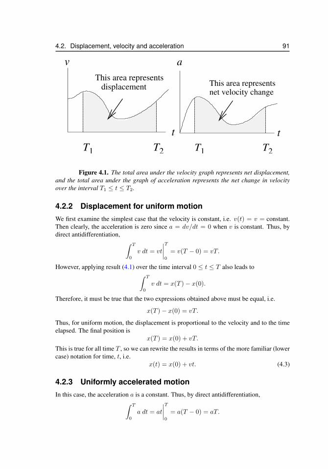
4.2. Displacement, velocity and acceleration 91
T T
v
1 2
t
displacementThis area represents
a
net velocity changeThis area represents
T1 T2
t
Figure 4.1. The total area under the velocity graph represents net displacement,and the total area under the graph of acceleration represents the net change in velocityover the interval T1 ≤ t ≤ T2.
4.2.2 Displacement for uniform motionWe first examine the simplest case that the velocity is constant, i.e. v(t) = v = constant.Then clearly, the acceleration is zero since a = dv/dt = 0 when v is constant. Thus, bydirect antidifferentiation, ∫ T
0
v dt = vt
∣∣∣∣T0
= v(T − 0) = vT.
However, applying result (4.1) over the time interval 0 ≤ t ≤ T also leads to∫ T
0
v dt = x(T )− x(0).
Therefore, it must be true that the two expressions obtained above must be equal, i.e.
x(T )− x(0) = vT.
Thus, for uniform motion, the displacement is proportional to the velocity and to the timeelapsed. The final position is
x(T ) = x(0) + vT.
This is true for all time T , so we can rewrite the results in terms of the more familiar (lowercase) notation for time, t, i.e.
x(t) = x(0) + vt. (4.3)
4.2.3 Uniformly accelerated motionIn this case, the acceleration a is a constant. Thus, by direct antidifferentiation,∫ T
0
a dt = at
∣∣∣∣T0
= a(T − 0) = aT.
92 Chapter 4. Applications of the definite integral to velocities and rates
However, using Equation (4.2) for 0 ≤ t ≤ T leads to∫ T
0
a dt = v(T )− v(0).
Since these two results must match, v(T )− v(0) = aT so that
v(T ) = v(0) + aT.
Let us refer to the initial velocity V (0) as v0. The above connection between velocity andacceleration holds for any final time T , i.e., it is true for all t that:
v(t) = v0 + at. (4.4)
This just means that velocity at time t is the initial velocity incremented by an increase (overthe given time interval) due to the acceleration. From this we can find the displacement andposition of the particle as follows: Let us call the initial position x(0) = x0. Then∫ T
0
v(t) dt = x(T )− x0. (4.5)
But
I =
∫ T
0
v(t) dt =
∫ T
0
(v0 + at) dt =
(v0t+ a
t2
2
) ∣∣∣∣T0
=
(v0T + a
T 2
2
). (4.6)
So, setting Equations (4.5) and (4.6) equal means that
x(T )− x0 = v0T + aT 2
2.
But this is true for all final times, T , i.e. this holds for any time t so that
x(t) = x0 + v0t+ at2
2. (4.7)
This expression represents the position of a particle at time t given that it experienced aconstant acceleration. The initial velocity v0, initial position x0 and acceleration a allowedus to predict the position of the object x(t) at any later time t. That is the meaning ofEqn. (4.7)17.
4.2.4 Non-constant acceleration and terminal velocityIn general, the acceleration of a falling body is not actually uniform, because frictionalforces impede that motion. A better approximation to the rate of change of velocity isgiven by the differential equation
dv
dt= g − kv. (4.8)
17Of course, Eqn. (4.7) only holds so long as the object is accelerating. Once the a falling object hits the ground,for example, this equation no longer holds.
4.2. Displacement, velocity and acceleration 93
We will assume that initially the velocity is zero, i.e. v(0) = 0.This equation is a mathematical statement that relates changes in velocity v(t) to the
constant acceleration due to gravity, g, and drag forces due to friction with the atmosphere.A good approximation for such drag forces is the term kv, proportional to the velocity,with k, a positive constant, representing a frictional coefficient. Because v(t) appears bothin the derivative and in the expression kv, we cannot apply the methods developed in theprevious section directly. That is, we do not have an expression that depends on time whoseantiderivative we would calculate. The derivative of v(t) (on the left) is connected to theunknown v(t) on the right.
Finding the velocity and then the displacement for this type of motion requires specialtechniques. In Chapter 9, we will develop a systematic approach, called Separation ofVariables to find analytic solutions to equations such as (4.8).
Here, we use a special procedure that allows us to determine the velocity in this case.We first recall the following result from first term calculus material:
The differential equation and initial condition
dy
dt= −ky, y(0) = y0 (4.9)
has a solutiony(t) = y0e
−kt. (4.10)
Equation (4.8) implies thata(t) = g − kv(t),
where a(t) is the acceleration at time t. Taking a derivative of both sides of this equationleads to
da
dt= −kdv
dt= −ka.
We observe that this equation has the same form as equation (4.9) (with a replacing y),which implies (according to 4.10) that a(t) is given by
a(t) = C e−kt = a0 e−kt.
Initially, at time t = 0, the acceleration is a(0) = g (since a(t) = g−kv(t), and v(0) = 0).Therefore,
a(t) = g e−kt.
Since we now have an explicit formula for acceleration vs time, we can apply direct inte-gration as we did in the examples in Sections 4.2.2 and 4.2.3. The result is:
∫ T
0
a(t) dt =
∫ T
0
g e−kt dt = g
∫ T
0
e−kt dt = g
[e−kt
−k
] ∣∣∣∣T0
= g(e−kT − 1)
−k=g
k
(1− e−kT
).
In the calculation, we have used the fact that the antiderivative of e−kt is −e−kt/k. (Thiscan be verified by simple differentiation.)
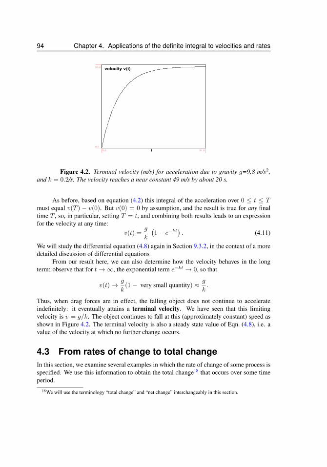
94 Chapter 4. Applications of the definite integral to velocities and rates
t
velocity v(t)
0.0 30.0
0.0
50.0
Figure 4.2. Terminal velocity (m/s) for acceleration due to gravity g=9.8 m/s2,and k = 0.2/s. The velocity reaches a near constant 49 m/s by about 20 s.
As before, based on equation (4.2) this integral of the acceleration over 0 ≤ t ≤ Tmust equal v(T ) − v(0). But v(0) = 0 by assumption, and the result is true for any finaltime T , so, in particular, setting T = t, and combining both results leads to an expressionfor the velocity at any time:
v(t) =g
k
(1− e−kt
). (4.11)
We will study the differential equation (4.8) again in Section 9.3.2, in the context of a moredetailed discussion of differential equations
From our result here, we can also determine how the velocity behaves in the longterm: observe that for t→∞, the exponential term e−kt → 0, so that
v(t)→ g
k(1− very small quantity) ≈ g
k.
Thus, when drag forces are in effect, the falling object does not continue to accelerateindefinitely: it eventually attains a terminal velocity. We have seen that this limitingvelocity is v = g/k. The object continues to fall at this (approximately constant) speed asshown in Figure 4.2. The terminal velocity is also a steady state value of Eqn. (4.8), i.e. avalue of the velocity at which no further change occurs.
4.3 From rates of change to total changeIn this section, we examine several examples in which the rate of change of some process isspecified. We use this information to obtain the total change18 that occurs over some timeperiod.
18We will use the terminology “total change” and “net change” interchangeably in this section.
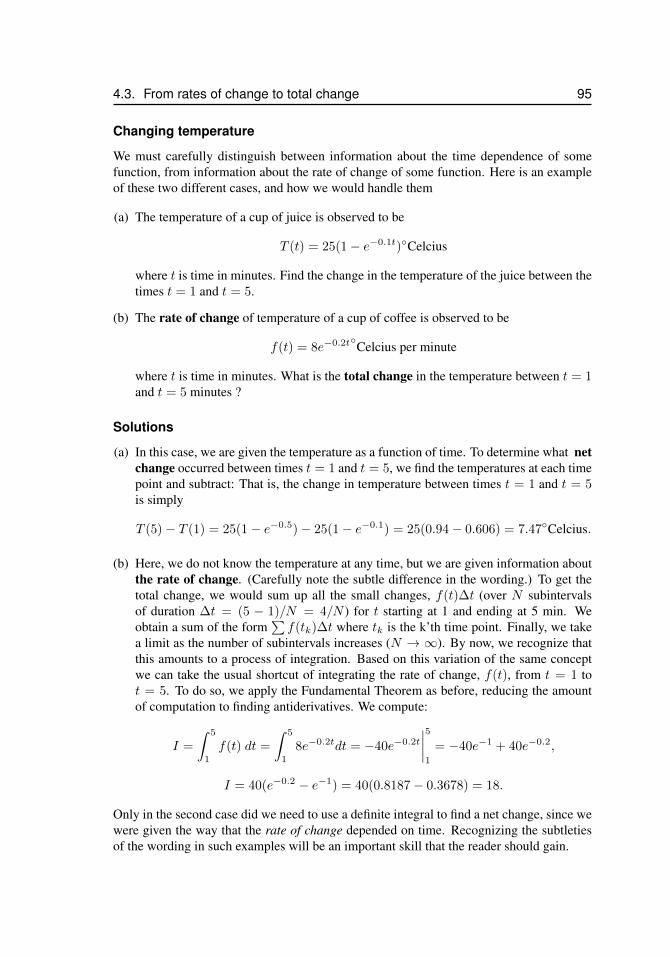
4.3. From rates of change to total change 95
Changing temperature
We must carefully distinguish between information about the time dependence of somefunction, from information about the rate of change of some function. Here is an exampleof these two different cases, and how we would handle them
(a) The temperature of a cup of juice is observed to be
T (t) = 25(1− e−0.1t)◦Celcius
where t is time in minutes. Find the change in the temperature of the juice between thetimes t = 1 and t = 5.
(b) The rate of change of temperature of a cup of coffee is observed to be
f(t) = 8e−0.2t◦Celcius per minute
where t is time in minutes. What is the total change in the temperature between t = 1and t = 5 minutes ?
Solutions
(a) In this case, we are given the temperature as a function of time. To determine what netchange occurred between times t = 1 and t = 5, we find the temperatures at each timepoint and subtract: That is, the change in temperature between times t = 1 and t = 5is simply
T (5)− T (1) = 25(1− e−0.5)− 25(1− e−0.1) = 25(0.94− 0.606) = 7.47◦Celcius.
(b) Here, we do not know the temperature at any time, but we are given information aboutthe rate of change. (Carefully note the subtle difference in the wording.) To get thetotal change, we would sum up all the small changes, f(t)∆t (over N subintervalsof duration ∆t = (5 − 1)/N = 4/N ) for t starting at 1 and ending at 5 min. Weobtain a sum of the form
∑f(tk)∆t where tk is the k’th time point. Finally, we take
a limit as the number of subintervals increases (N → ∞). By now, we recognize thatthis amounts to a process of integration. Based on this variation of the same conceptwe can take the usual shortcut of integrating the rate of change, f(t), from t = 1 tot = 5. To do so, we apply the Fundamental Theorem as before, reducing the amountof computation to finding antiderivatives. We compute:
I =
∫ 5
1
f(t) dt =
∫ 5
1
8e−0.2tdt = −40e−0.2t
∣∣∣∣51
= −40e−1 + 40e−0.2,
I = 40(e−0.2 − e−1) = 40(0.8187− 0.3678) = 18.
Only in the second case did we need to use a definite integral to find a net change, since wewere given the way that the rate of change depended on time. Recognizing the subtletiesof the wording in such examples will be an important skill that the reader should gain.
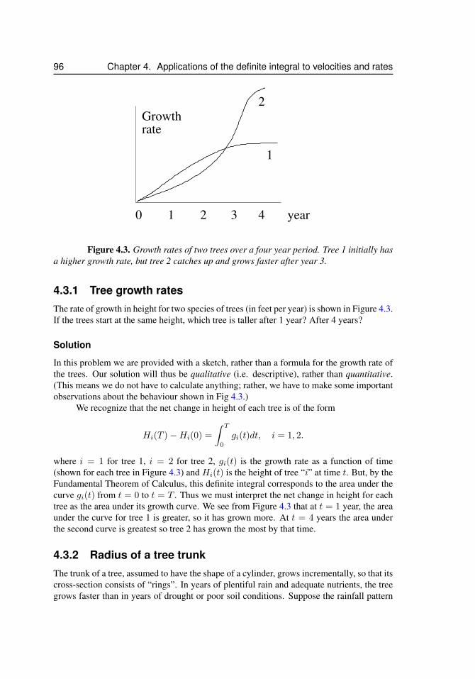
96 Chapter 4. Applications of the definite integral to velocities and rates
2
0 1 2 3
1
rateGrowth
4 year
Figure 4.3. Growth rates of two trees over a four year period. Tree 1 initially hasa higher growth rate, but tree 2 catches up and grows faster after year 3.
4.3.1 Tree growth ratesThe rate of growth in height for two species of trees (in feet per year) is shown in Figure 4.3.If the trees start at the same height, which tree is taller after 1 year? After 4 years?
Solution
In this problem we are provided with a sketch, rather than a formula for the growth rate ofthe trees. Our solution will thus be qualitative (i.e. descriptive), rather than quantitative.(This means we do not have to calculate anything; rather, we have to make some importantobservations about the behaviour shown in Fig 4.3.)
We recognize that the net change in height of each tree is of the form
Hi(T )−Hi(0) =
∫ T
0
gi(t)dt, i = 1, 2.
where i = 1 for tree 1, i = 2 for tree 2, gi(t) is the growth rate as a function of time(shown for each tree in Figure 4.3) and Hi(t) is the height of tree “i” at time t. But, by theFundamental Theorem of Calculus, this definite integral corresponds to the area under thecurve gi(t) from t = 0 to t = T . Thus we must interpret the net change in height for eachtree as the area under its growth curve. We see from Figure 4.3 that at t = 1 year, the areaunder the curve for tree 1 is greater, so it has grown more. At t = 4 years the area underthe second curve is greatest so tree 2 has grown the most by that time.
4.3.2 Radius of a tree trunkThe trunk of a tree, assumed to have the shape of a cylinder, grows incrementally, so that itscross-section consists of “rings”. In years of plentiful rain and adequate nutrients, the treegrows faster than in years of drought or poor soil conditions. Suppose the rainfall pattern
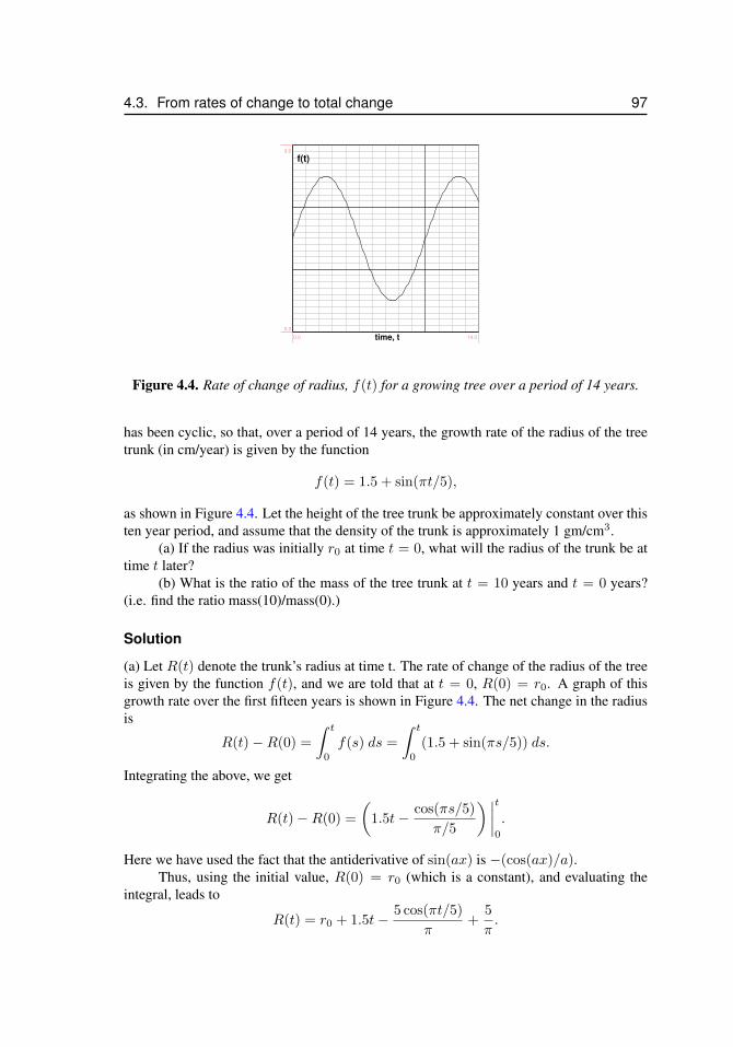
4.3. From rates of change to total change 97
time, t
f(t)
0.0 14.0
0.0
3.0
Figure 4.4. Rate of change of radius, f(t) for a growing tree over a period of 14 years.
has been cyclic, so that, over a period of 14 years, the growth rate of the radius of the treetrunk (in cm/year) is given by the function
f(t) = 1.5 + sin(πt/5),
as shown in Figure 4.4. Let the height of the tree trunk be approximately constant over thisten year period, and assume that the density of the trunk is approximately 1 gm/cm3.
(a) If the radius was initially r0 at time t = 0, what will the radius of the trunk be attime t later?
(b) What is the ratio of the mass of the tree trunk at t = 10 years and t = 0 years?(i.e. find the ratio mass(10)/mass(0).)
Solution
(a) Let R(t) denote the trunk’s radius at time t. The rate of change of the radius of the treeis given by the function f(t), and we are told that at t = 0, R(0) = r0. A graph of thisgrowth rate over the first fifteen years is shown in Figure 4.4. The net change in the radiusis
R(t)−R(0) =
∫ t
0
f(s) ds =
∫ t
0
(1.5 + sin(πs/5)) ds.
Integrating the above, we get
R(t)−R(0) =
(1.5t− cos(πs/5)
π/5
) ∣∣∣∣t0
.
Here we have used the fact that the antiderivative of sin(ax) is −(cos(ax)/a).Thus, using the initial value, R(0) = r0 (which is a constant), and evaluating the
integral, leads to
R(t) = r0 + 1.5t− 5 cos(πt/5)
π+
5
π.
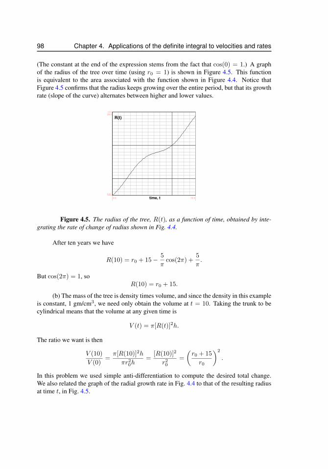
98 Chapter 4. Applications of the definite integral to velocities and rates
(The constant at the end of the expression stems from the fact that cos(0) = 1.) A graphof the radius of the tree over time (using r0 = 1) is shown in Figure 4.5. This functionis equivalent to the area associated with the function shown in Figure 4.4. Notice thatFigure 4.5 confirms that the radius keeps growing over the entire period, but that its growthrate (slope of the curve) alternates between higher and lower values.
time, t
R(t)
0.0 14.0
0.0
25.0
Figure 4.5. The radius of the tree, R(t), as a function of time, obtained by inte-grating the rate of change of radius shown in Fig. 4.4.
After ten years we have
R(10) = r0 + 15− 5
πcos(2π) +
5
π.
But cos(2π) = 1, soR(10) = r0 + 15.
(b) The mass of the tree is density times volume, and since the density in this exampleis constant, 1 gm/cm3, we need only obtain the volume at t = 10. Taking the trunk to becylindrical means that the volume at any given time is
V (t) = π[R(t)]2h.
The ratio we want is then
V (10)
V (0)=π[R(10)]2h
πr20h
=[R(10)]2
r20
=
(r0 + 15
r0
)2
.
In this problem we used simple anti-differentiation to compute the desired total change.We also related the graph of the radial growth rate in Fig. 4.4 to that of the resulting radiusat time t, in Fig. 4.5.

4.4. Production and removal 99
4.3.3 Birth rates and total birthsAfter World War II, the birth rate in western countries increased dramatically. Suppose thatthe number of babies born (in millions per year) was given by
b(t) = 5 + 2t, 0 ≤ t ≤ 10,
where t is time in years after the end of the war.
(a) How many babies in total were born during this time period (i.e in the first 10 yearsafter the war)?
(b) Find the time T0 such that the total number of babies born from the end of the war upto the time T0 was precisely 14 million.
Solution
(a) To find the number of births, we would integrate the birth rate, b(t) over the given timeperiod. The net change in the population due to births (neglecting deaths) is
P (10)−P (0) =
∫ 10
0
b(t) dt =
∫ 10
0
(5+2t) dt = (5t+t2)|100 = 50+100 = 150[million babies].
(b) Denote by T the time at which the total number of babies born was 14 million. Then,[in units of million]
I =
∫ T
0
b(t) dt = 14 =
∫ T
0
(5 + 2t) dt = 5T + T 2
equating I = 14 leads to the quadratic equation, T 2 + 5T − 14 = 0, which can bewritten in the factored form, (T −2)(T + 7) = 0. This has two solutions, but we rejectT = −7 since we are looking for time after the War. Thus we find that T = 2 years,i.e it took two years for 14 million babies to have been born.
While this problem involves simple integration, we had to solve for a quantity (T ) basedon information about behaviour of that integral. Many problems in real application involvesuch slight twists on the ideas of integration.
4.4 Production and removalThe process of integration can be used to convert rates of production and removal into netamounts present at a given time. The example in this section is of this type. We investigatea process in which a substance accumulates as it is being produced, but disappears throughsome removal process. We would like to determine when the quantity of material increases,and when it decreases.
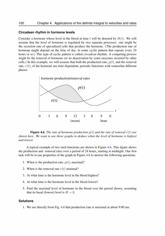
100 Chapter 4. Applications of the definite integral to velocities and rates
Circadean rhythm in hormone levels
Consider a hormone whose level in the blood at time t will be denoted by H(t). We willassume that the level of hormone is regulated by two separate processes: one might bethe secretion rate of specialized cells that produce the hormone. (The production rate ofhormone might depend on the time of day, in some cyclic pattern that repeats every 24hours or so.) This type of cyclic pattern is called circadean rhythm. A competing processmight be the removal of hormone (or its deactivation by some enzymes secreted by othercells.) In this example, we will assume that both the production rate, p(t), and the removalrate, r(t), of the hormone are time-dependent, periodic functions with somewhat differentphases.
126 60 0
(noon)
3 3 99
r(t)
hour
hormone production/removal rates
t
p(t)
Figure 4.6. The rate of hormone production p(t) and the rate of removal r(t) areshown here. We want to use these graphs to deduce when the level of hormone is highestand lowest.
A typical example of two such functions are shown in Figure 4.6. This figure showsthe production and removal rates over a period of 24 hours, starting at midnight. Our firsttask will be to use properties of the graph in Figure 4.6 to answer the following questions:
1. When is the production rate, p(t), maximal?
2. When is the removal rate r(t) minimal?
3. At what time is the hormone level in the blood highest?
4. At what time is the hormone level in the blood lowest?
5. Find the maximal level of hormone in the blood over the period shown, assumingthat its basal (lowest) level is H = 0.
Solutions
1. We see directly from Fig. 4.6 that production rate is maximal at about 9:00 am.
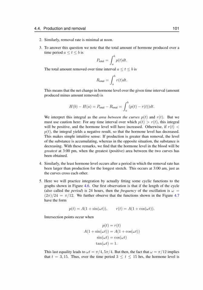
4.4. Production and removal 101
2. Similarly, removal rate is minimal at noon.
3. To answer this question we note that the total amount of hormone produced over atime period a ≤ t ≤ b is
Ptotal =
∫ b
a
p(t)dt.
The total amount removed over time interval a ≤ t ≤ b is
Rtotal =
∫ b
a
r(t)dt.
This means that the net change in hormone level over the given time interval (amountproduced minus amount removed) is
H(b)−H(a) = Ptotal −Rtotal =
∫ b
a
(p(t)− r(t))dt.
We interpret this integral as the area between the curves p(t) and r(t). But wemust use caution here: For any time interval over which p(t) > r(t), this integralwill be positive, and the hormone level will have increased. Otherwise, if r(t) <p(t), the integral yields a negative result, so that the hormone level has decreased.This makes simple intuitive sense: If production is greater than removal, the levelof the substance is accumulating, whereas in the opposite situation, the substance isdecreasing. With these remarks, we find that the hormone level in the blood will begreatest at 3:00 pm, when the greatest (positive) area between the two curves hasbeen obtained.
4. Similarly, the least hormone level occurs after a period in which the removal rate hasbeen larger than production for the longest stretch. This occurs at 3:00 am, just asthe curves cross each other.
5. Here we will practice integration by actually fitting some cyclic functions to thegraphs shown in Figure 4.6. Our first observation is that if the length of the cycle(also called the period) is 24 hours, then the frequency of the oscillation is ω =(2π)/24 = π/12. We further observe that the functions shown in the Figure 4.7have the form
p(t) = A(1 + sin(ωt)), r(t) = A(1 + cos(ωt)).
Intersection points occur when
p(t) = r(t)
A(1 + sin(ωt)) = A(1 + cos(ωt))
sin(ωt) = cos(ωt)
tan(ωt) = 1.
This last equality leads to ωt = π/4, 5π/4. But then, the fact that ω = π/12 impliesthat t = 3, 15. Thus, over the time period 3 ≤ t ≤ 15 hrs, the hormone level is
102 Chapter 4. Applications of the definite integral to velocities and rates
0
0.5
1
1.5
2
5 10 15 20t
Figure 4.7. The functions shown above are trigonometric approximations to therates of hormone production and removal from Figure 4.6
increasing. For simplicity, we will take the amplitude A = 1. (In general, this wouldjust be a multiplicative constant in whatever solution we compute.) Then the netincrease in hormone over this period is calculated from the integral
Htotal =
∫ 15
3
[p(t)− r(t)] dt =
∫ 15
3
[(1 + sin(ωt))− (1 + cos(ωt))] dt
In the problem set, the reader is asked to compute this integral and to show that theamount of hormone that accumulated over the time interval 3 ≤ t ≤ 15, i.e. between3:00 am and 3:00 pm is 24
√2/π.
4.5 Average value of a functionIn this final example, we apply the definite integral to computing the average height ofa function over some interval. First, we define what is meant by average value in thiscontext.19
Given a functiony = f(x)
over some interval a ≤ x ≤ b, we will define average value of the function as follows:
Definition
The average value of f(x) over the interval a ≤ x ≤ b is
f =1
b− a
∫ b
a
f(x)dx. (4.12)
19In Chapters 5 and 8, we will encounter a different type of average (also called mean) that will represent anaverage horizontal position or center of mass. It is important to avoid confusing these distinct notions.
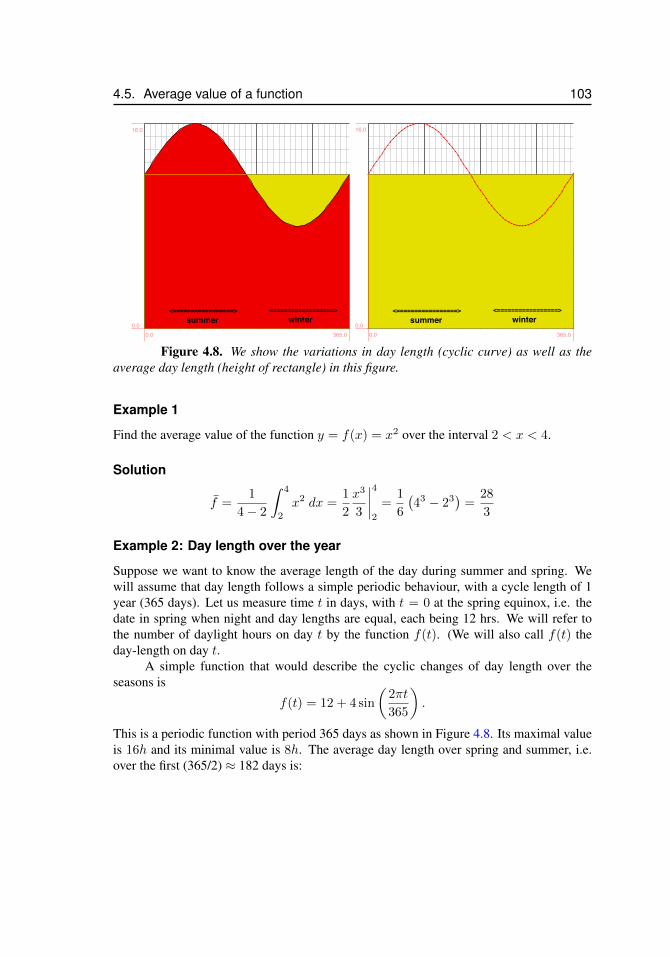
4.5. Average value of a function 103
summer winter<=================> <=================>
0.0 365.00.0
16.0
summer winter<=================> <=================>
0.0 365.00.0
16.0
Figure 4.8. We show the variations in day length (cyclic curve) as well as theaverage day length (height of rectangle) in this figure.
Example 1
Find the average value of the function y = f(x) = x2 over the interval 2 < x < 4.
Solution
f =1
4− 2
∫ 4
2
x2 dx =1
2
x3
3
∣∣∣∣42
=1
6
(43 − 23
)=
28
3
Example 2: Day length over the year
Suppose we want to know the average length of the day during summer and spring. Wewill assume that day length follows a simple periodic behaviour, with a cycle length of 1year (365 days). Let us measure time t in days, with t = 0 at the spring equinox, i.e. thedate in spring when night and day lengths are equal, each being 12 hrs. We will refer tothe number of daylight hours on day t by the function f(t). (We will also call f(t) theday-length on day t.
A simple function that would describe the cyclic changes of day length over theseasons is
f(t) = 12 + 4 sin
(2πt
365
).
This is a periodic function with period 365 days as shown in Figure 4.8. Its maximal valueis 16h and its minimal value is 8h. The average day length over spring and summer, i.e.over the first (365/2) ≈ 182 days is:
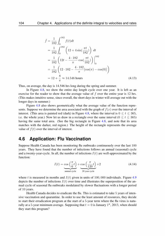
104 Chapter 4. Applications of the definite integral to velocities and rates
f =1
182
∫ 182
0
f(t)dt
=1
182
∫ 182
0
(12 + 4 sin(
πt
182)
)dt
=1
182
(12t− 4 · 182
πcos(
πt
182)
) ∣∣∣∣182
0
=1
182
(12 · 182− 4 · 182
π[cos(π)− cos(0)]
)= 12 +
8
π≈ 14.546 hours (4.13)
Thus, on average, the day is 14.546 hrs long during the spring and summer.In Figure 4.8, we show the entire day length cycle over one year. It is left as an
exercise for the reader to show that the average value of f over the entire year is 12 hrs.(This makes intuitive sense, since overall, the short days in winter will average out with thelonger days in summer.)
Figure 4.8 also shows geometrically what the average value of the function repre-sents. Suppose we determine the area associated with the graph of f(x) over the interval ofinterest. (This area is painted red (dark) in Figure 4.8, where the interval is 0 ≤ t ≤ 365,i.e. the whole year.) Now let us draw in a rectangle over the same interval (0 ≤ t ≤ 365)having the same total area. (See the big rectangle in Figure 4.8, and note that its areamatches with the darker, red region.) The height of the rectangle represents the averagevalue of f(t) over the interval of interest.
4.6 Application: Flu VaccinationSuppose Health Canada has been monitoring flu outbreaks continuously over the last 100years. They have found that the number of infections follows an annual (seasonal) cycleand a twenty-year-cycle. In all, the number of infections I(t) are well-approximated by thefunction:
I(t) = cos(π
6t)
︸ ︷︷ ︸annual cycle
+ cos( π
120t)
︸ ︷︷ ︸20 year cycle
+2 (4.14)
where t is measured in months and I(t) given in units of 100, 000 individuals. Figure 4.9depicts the number of infections I(t) over time and illustrates the superposition of the an-nual cycle of seasonal flu outbreaks modulated by slower fluctuations with a longer periodof 10 years.
Health Canada decides to eradicate the flu. This is estimated to take 5 years of inten-sive vaccination and quarantine. In order to use the least amount of resources, they decideto start their erradication program at the start of a 5-year term where the flu virus is natu-rally at a 5-year minimum average. Supposing that t = 0 is January 1st, 2013, when shouldthey start this program?
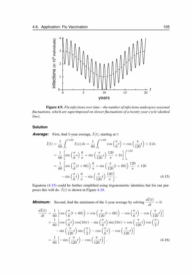
4.6. Application: Flu Vaccination 105
5 10 15 20
1
2
3
4
t
years0
0infe
ctio
ns (in
105 in
divi
dual
s)
Figure 4.9. Flu infections over time – the number of infections undergoes seasonalfluctuations, which are superimposed on slower fluctuations of a twenty-year-cycle (dashedline).
Solution
Average: First, find 5-year average, I(t), starting at t:
I(t) =1
60
∫ t+60
t
I(s) ds =1
60
∫ t+60
t
cos(π
6t)
+ cos( π
120t)
+ 2 ds
=1
60
[sin(π
6s) 6
π+ sin
( π
120s) 120
π+ 2s
] ∣∣∣∣t+60
t
=1
60
[sin(π
6(t+ 60)
) 6
π+ sin
( π
120(t+ 60)
) 120
π+ 120
− sin(π
6t) 6
π− sin
( π
120t) 120
π
]. (4.15)
Equation (4.15) could be further simplified using trigonometric identities but for our pur-poses this will do. I(t) is shown in Figure 4.10.
Minimum: Second, find the minimum of the 5-year average by solvingdI(t)
dt= 0:
dI(t)
dt=
1
60
[cos(π
6(t+ 60)
)+ cos
( π
120(t+ 60)
)− cos
(π6t)− cos
( π
120t)]
=1
60
[cos(π
6t)
cos(10π)− sin(π
6t)
sin(10π) + cos( π
120t)
cos(π
2
)− sin
( π
120t)
sin(π
2
)− cos
(π6t)− cos
( π
120t)]
=1
60
[− sin
( π
120t)− cos
( π
120t)]. (4.16)
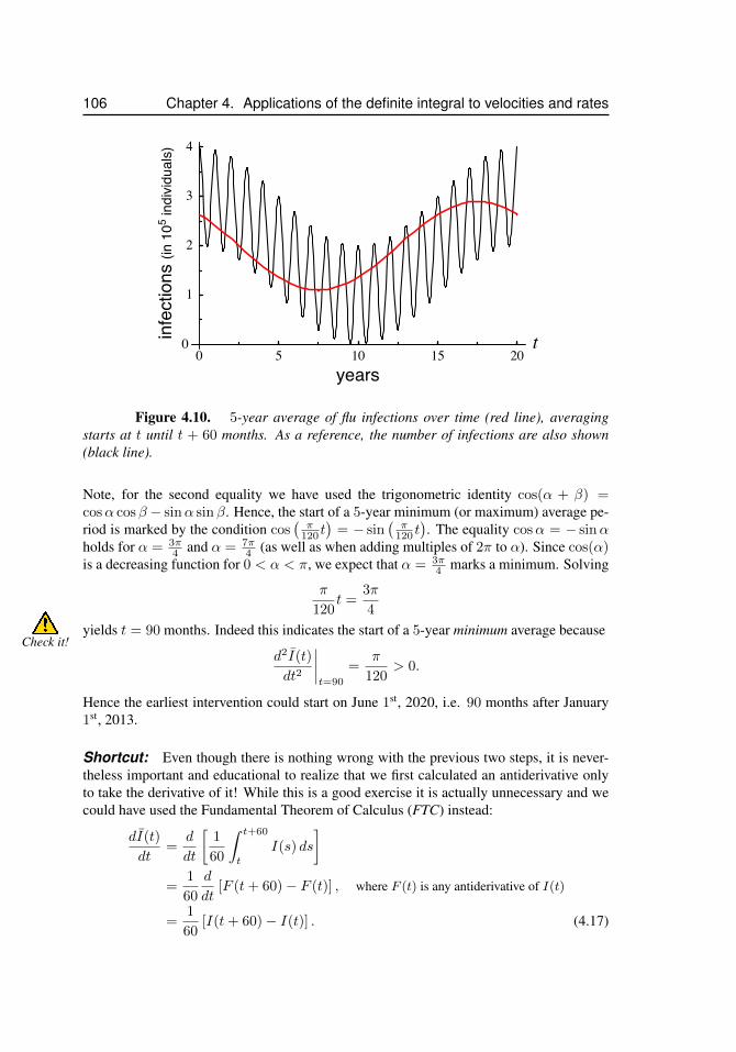
106 Chapter 4. Applications of the definite integral to velocities and rates
5 10 15 20
1
2
3
4
t
years0
0infe
ctio
ns (in
105 in
divi
dual
s)
Figure 4.10. 5-year average of flu infections over time (red line), averagingstarts at t until t + 60 months. As a reference, the number of infections are also shown(black line).
Note, for the second equality we have used the trigonometric identity cos(α + β) =cosα cosβ − sinα sinβ. Hence, the start of a 5-year minimum (or maximum) average pe-riod is marked by the condition cos
(π
120 t)
= − sin(π
120 t). The equality cosα = − sinα
holds for α = 3π4 and α = 7π
4 (as well as when adding multiples of 2π to α). Since cos(α)is a decreasing function for 0 < α < π, we expect that α = 3π
4 marks a minimum. Solving
π
120t =
3π
4
yields t = 90 months. Indeed this indicates the start of a 5-year minimum average becauseCheck it!
d2I(t)
dt2
∣∣∣∣t=90
=π
120> 0.
Hence the earliest intervention could start on June 1st, 2020, i.e. 90 months after January1st, 2013.
Shortcut: Even though there is nothing wrong with the previous two steps, it is never-theless important and educational to realize that we first calculated an antiderivative onlyto take the derivative of it! While this is a good exercise it is actually unnecessary and wecould have used the Fundamental Theorem of Calculus (FTC) instead:
dI(t)
dt=
d
dt
[1
60
∫ t+60
t
I(s) ds
]=
1
60
d
dt[F (t+ 60)− F (t)] , where F (t) is any antiderivative of I(t)
=1
60[I(t+ 60)− I(t)] . (4.17)
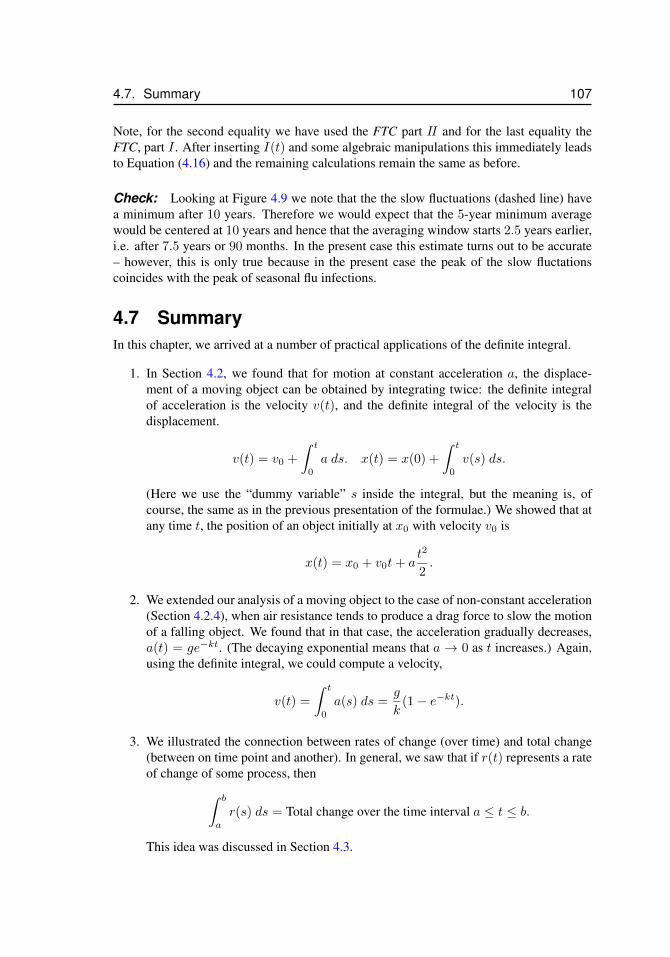
4.7. Summary 107
Note, for the second equality we have used the FTC part II and for the last equality theFTC, part I . After inserting I(t) and some algebraic manipulations this immediately leadsto Equation (4.16) and the remaining calculations remain the same as before.
Check: Looking at Figure 4.9 we note that the the slow fluctuations (dashed line) havea minimum after 10 years. Therefore we would expect that the 5-year minimum averagewould be centered at 10 years and hence that the averaging window starts 2.5 years earlier,i.e. after 7.5 years or 90 months. In the present case this estimate turns out to be accurate– however, this is only true because in the present case the peak of the slow fluctationscoincides with the peak of seasonal flu infections.
4.7 SummaryIn this chapter, we arrived at a number of practical applications of the definite integral.
1. In Section 4.2, we found that for motion at constant acceleration a, the displace-ment of a moving object can be obtained by integrating twice: the definite integralof acceleration is the velocity v(t), and the definite integral of the velocity is thedisplacement.
v(t) = v0 +
∫ t
0
a ds. x(t) = x(0) +
∫ t
0
v(s) ds.
(Here we use the “dummy variable” s inside the integral, but the meaning is, ofcourse, the same as in the previous presentation of the formulae.) We showed that atany time t, the position of an object initially at x0 with velocity v0 is
x(t) = x0 + v0t+ at2
2.
2. We extended our analysis of a moving object to the case of non-constant acceleration(Section 4.2.4), when air resistance tends to produce a drag force to slow the motionof a falling object. We found that in that case, the acceleration gradually decreases,a(t) = ge−kt. (The decaying exponential means that a → 0 as t increases.) Again,using the definite integral, we could compute a velocity,
v(t) =
∫ t
0
a(s) ds =g
k(1− e−kt).
3. We illustrated the connection between rates of change (over time) and total change(between on time point and another). In general, we saw that if r(t) represents a rateof change of some process, then∫ b
a
r(s) ds = Total change over the time interval a ≤ t ≤ b.
This idea was discussed in Section 4.3.

108 Chapter 4. Applications of the definite integral to velocities and rates
4. In the concluding Section 4.5, we discussed the average value of a function f(x)over some interval a ≤ x ≤ b,
f =1
b− a
∫ b
a
f(x)dx.
In the next few chapters we encounters a vast assortment of further examples andpractical applications of the definite integral, to such topics as mass, volumes, length,etc. In some of these we will be called on to “dissect” a geometric shape into piecesthat are not simple rectangles. The essential idea of an integral as a sum of many(infinitesimally) small pieces will, nevertheless be the same.
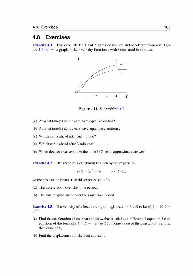
4.8. Exercises 109
4.8 ExercisesExercise 4.1 Two cars, labeled 1 and 2 start side by side and accelerate from rest. Fig-ure 4.11 shows a graph of their velocity functions, with t measured in minutes.
2
2 31 4 t
v
1
Figure 4.11. For problem 4.1
(a) At what time(s) do the cars have equal velocities?
(b) At what time(s) do the cars have equal accelerations?
(c) Which car is ahead after one minute?
(d) Which car is ahead after 3 minutes?
(e) When does one car overtake the other? (Give an approximate answer)
Exercise 4.2 The speed of a car (km/h) is given by the expression
v(t) = 2t2 + 5t, 0 < t < 1
where t is time in hours. Use this expression to find
(a) The acceleration over this time period.
(b) The total displacement over the same time period.
Exercise 4.3 The velocity of a boat moving through water is found to be v(t) = 10(1 −e−t).
(a) Find the acceleration of the boat and show that it satisfies a differential equation, i.e anequation of the form d[a(t)]/dt = −k · a(t) for some value of the constant k (i.e. findthat value of k).
(b) Find the displacement of the boat at time t.
110 Chapter 4. Applications of the definite integral to velocities and rates
Exercise 4.4 A particle in a force field accelerates so that its acceleration is described bythe function
a(t) = t− t2, 0 < t < 1
(a) Find the velocity of the particle v(t) for 0 < t < 1 assuming that it starts at rest.
(b) Find the total displacement of the particle over the time interval 0 < t < 1.
Exercise 4.5 An express mail truck delivers mail to various companies situated along acentral avenue and often goes back and forth as new mail arrives. Over some period oftime, 0 < t < 10, its velocity (in km per hour) can be described by the function:
v(t) = t2 − 9t+ 14.
(a) Find the displacement over this period of time. (Hint: recall that if you leave home inthe morning, travel to work, and then go back home, then your net distance traveled,or total displacement, over this full period of time is zero.)
(b) How much gasoline was consumed during this period of time if the vehicle uses 1/2liters per km. (Hint: To answer (b), you will need to find the total distance that thevehicle actually covered during its trip.)
Exercise 4.6 The reaction time of a driver (time it takes to notice and react to danger inthe road ahead) is about 0.5 seconds. When the brakes are applied, it then takes the carsome time to decelerate and come to a full stop. If the deceleration rate is a = −8 m/sec2,how long would it take the driver to stop from an initial speed of 100 km per hour? (Includeboth reaction time and deceleration time, and use the Fundamental Theorem of Calculus toarrive at your answer.)
Exercise 4.7 You are driving your car quickly (at speed 100 km/h) to catch your flight toHawaii for mid-term break. A pedestrian runs across the road, forcing you to brake hard.Suppose it takes you 1 second to react to the danger, and that when you apply your brakes,you slow down at the rate a = −10 m/s2.
(a) How long will it take you to stop?
(b) How far will your car move from the instant that the danger is sighted until coming toa complete stop?
Use the Fundamental Theorem of Calculus to arrive at your answer.
Exercise 4.8 The growth rate of a pair of twins (in mm/day) is shown in Figure 4.12.Suppose both children have the same weight at time t = 0.
(a) Which one is taller at age 0.5 years?
(b) Which one is taller at age 1 year?
4.8. Exercises 111
2
0 10.5 years
growth
rate1
Figure 4.12. For problem 4.8
Exercise 4.9 The flow rate of blood through the heart can be described approximately asa periodic function of the form F (t) = A(1 + sin(0.15t)), where t is time in seconds andA is a constant in units of cubic cm per second. (Thus, at time t, F (t) cm3 of blood flowthrough the heart per second.) Find the total volume of blood that flows through the heartbetween t = 0 and t = 1. (Express your answer in terms of A.)
Exercise 4.10 During a gambling session lasting 6 hours, the rate of winnings at a casinoin dollars per hour are seen to follow the formula w(t) = 2000t(1− (t/6)). Find the totalwinnings during that whole session.
Exercise 4.11 At time t, an intravenous infusion delivers a flow rate of y = 100(1 −t3) cm3/hr, where t is time in hours. The infusion contains a drug at concentration0.1 mg/cm3. Find the total volume of fluid and the total amount of drug delivered tothe patient over a 1 hour period from t = 0 to t = 1.
Exercise 4.12 Oil leaks out of an oil tanker at the rate f(t) = 10 − 0.2t2 (where f is in10 thousand barrels per hour and t is in hours). (Note: This function only makes sense aslong as f(t) ≥ 0 since a negative flow of oil is meaningless in this case.)
(a) At what time will the flow be zero?
(b) What is the total amount that has leaked out between t = 0 and the time you found in(a)?
Exercise 4.13 After a heavy rainfall, the rate of flow of water into a lake is found to
satisfy the relationship F (t) = 4 −(t
10− 1
)2
where t is time in hours, 0 ≤ t ≤ 30 and
F is in units of 100,000 gallons/h.
(a) Find the time, t1 at which the rate of flow is greatest.

112 Chapter 4. Applications of the definite integral to velocities and rates
(b) Find the time, t2 at which the flow is zero.
(c) Find how much water in total has flowed into the lake between these two times.
Exercise 4.14 The growth rate of a crop is known to depend on temperature during thegrowing season. Suppose the growth rate of the crop in tons per day is given by g(t) =0.1(T (t) − 18) where T (t) is temperature in degrees Celsius. Suppose the temperaturerecord during the 90 days of the season was T (t) = 22 + 0.1t + 4 sin(2πt/60) where tis time in days. Find the total growth (in tons) that would have occurred over the wholeseason.
Exercise 4.15 This question concerns cumulative exposure to radiation experienced bypeople living near nuclear waste disposal sites.
(a) Recall from last term that radioactive material decays according to a negative exponen-tial: m(t) = m0 · e−rt, where m(t) is the mass of the radioactive material at time t,m0 = m(0) is the initial mass at time t = 0, and r is the rate of decay. The half-life isthe time it takes for the material to decay to one half its initial mass. Suppose that t ismeasured in months. Determine the rate of decay r if the half-life is 1 month.
(b) Assume that at any time, the amount of radiation is proportional to the mass of theradioactive material. If initially the radiation level is 0.5 rads per month, how could wedescribe the radiation level as a function of time?
(c) Assume now that there is radioactive material in your backyard of the type consideredin (a) above, i.e. that it has a half-life of one month. Calculate the cumulative exposurein rads that would occur if you lived in your house for 10 years.
Exercise 4.16 The level of glucose in the blood depends on the rate of intake from inges-tion of food and on the rate of clearance due to glucose metabolism. Shown in Figure 4.13are two functions, I(t) and C(t) for the intake and clearance rates over a period of timeafter fasting. Both rates are functions of time t. Suppose that at time 0 there is no glucosein the blood.
(a) Express the level of blood glucose as a definite integral.
(b) At what approximate time was the intake rate maximal?
(c) At what approximate time was the clearance rate maximal?
(d) When was the blood level of glucose maximal?
Exercise 4.17 The rate at which water flows in and out of Capilano Reservoir is describedby two functions. I(t) is the rate at which water flows in to the reservoir (in gallons perday) and O(t) is the rate at which water flows out (in gallons per day). See sketch below inFigure 4.14. Assume that there is water in the reservoir at time t = 0.
(a) Express the quantity of water Q(t) in the reservoir as a definite integral. (i.e. Q(0) >0).
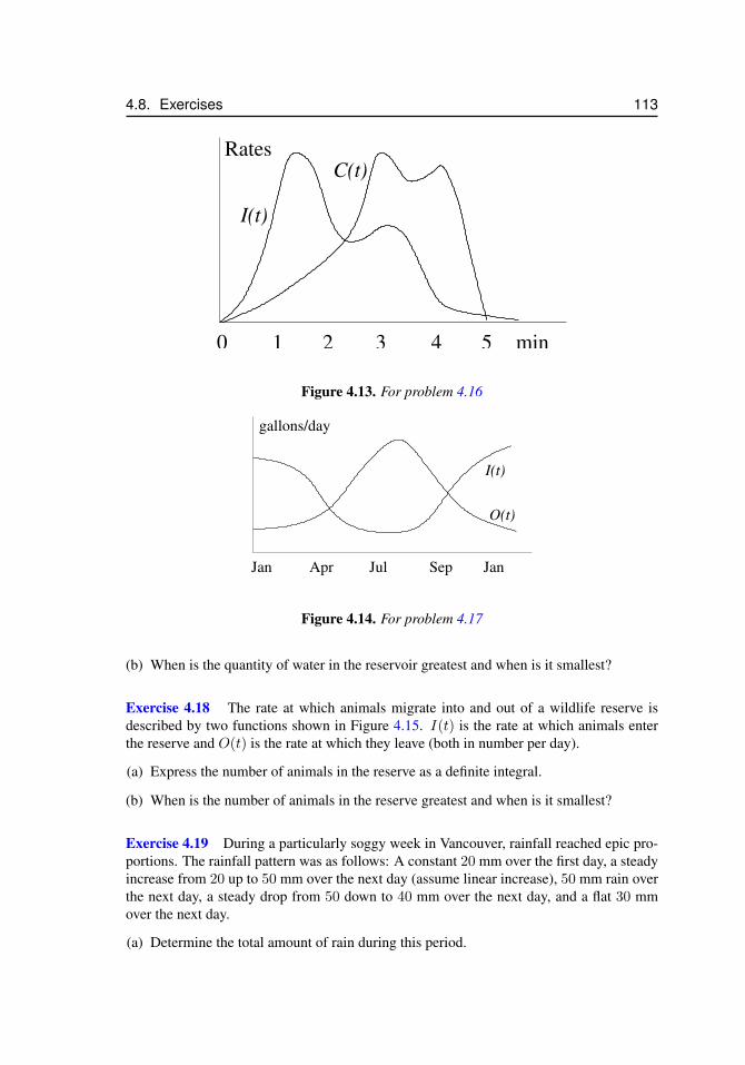
4.8. Exercises 113
C(t)
3 4 50 1
Rates
I(t)
2 min
Figure 4.13. For problem 4.16
O(t)
Jan Apr JanJul Sep
gallons/day
I(t)
Figure 4.14. For problem 4.17
(b) When is the quantity of water in the reservoir greatest and when is it smallest?
Exercise 4.18 The rate at which animals migrate into and out of a wildlife reserve isdescribed by two functions shown in Figure 4.15. I(t) is the rate at which animals enterthe reserve and O(t) is the rate at which they leave (both in number per day).
(a) Express the number of animals in the reserve as a definite integral.
(b) When is the number of animals in the reserve greatest and when is it smallest?
Exercise 4.19 During a particularly soggy week in Vancouver, rainfall reached epic pro-portions. The rainfall pattern was as follows: A constant 20 mm over the first day, a steadyincrease from 20 up to 50 mm over the next day (assume linear increase), 50 mm rain overthe next day, a steady drop from 50 down to 40 mm over the next day, and a flat 30 mmover the next day.
(a) Determine the total amount of rain during this period.
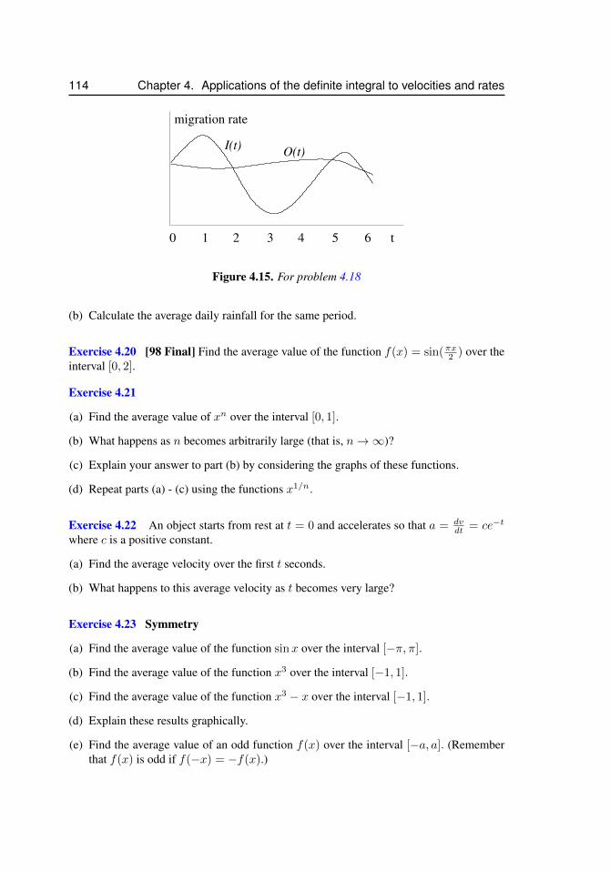
114 Chapter 4. Applications of the definite integral to velocities and rates
t0 1 2 3 4 5 6
I(t)O(t)
migration rate
Figure 4.15. For problem 4.18
(b) Calculate the average daily rainfall for the same period.
Exercise 4.20 [98 Final] Find the average value of the function f(x) = sin(πx2 ) over theinterval [0, 2].
Exercise 4.21
(a) Find the average value of xn over the interval [0, 1].
(b) What happens as n becomes arbitrarily large (that is, n→∞)?
(c) Explain your answer to part (b) by considering the graphs of these functions.
(d) Repeat parts (a) - (c) using the functions x1/n.
Exercise 4.22 An object starts from rest at t = 0 and accelerates so that a = dvdt = ce−t
where c is a positive constant.
(a) Find the average velocity over the first t seconds.
(b) What happens to this average velocity as t becomes very large?
Exercise 4.23 Symmetry
(a) Find the average value of the function sinx over the interval [−π, π].
(b) Find the average value of the function x3 over the interval [−1, 1].
(c) Find the average value of the function x3 − x over the interval [−1, 1].
(d) Explain these results graphically.
(e) Find the average value of an odd function f(x) over the interval [−a, a]. (Rememberthat f(x) is odd if f(−x) = −f(x).)
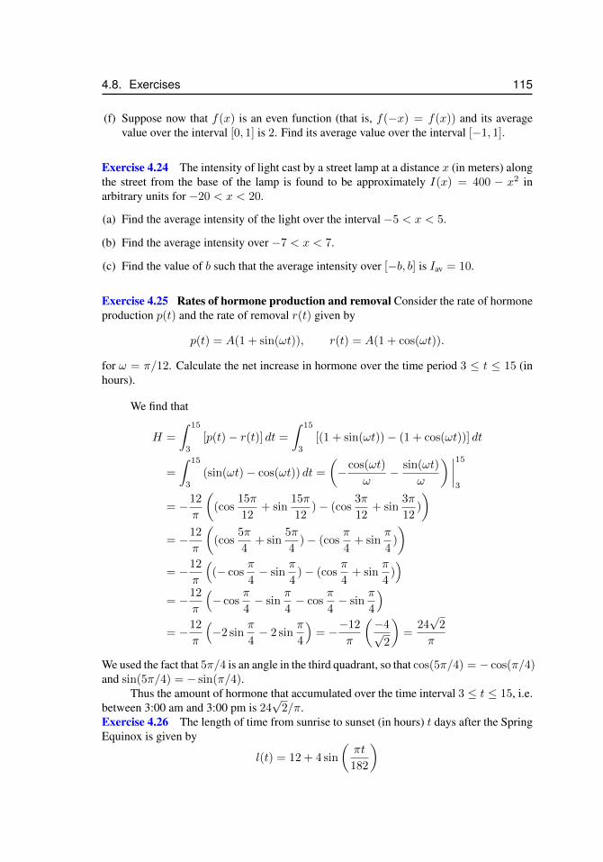
4.8. Exercises 115
(f) Suppose now that f(x) is an even function (that is, f(−x) = f(x)) and its averagevalue over the interval [0, 1] is 2. Find its average value over the interval [−1, 1].
Exercise 4.24 The intensity of light cast by a street lamp at a distance x (in meters) alongthe street from the base of the lamp is found to be approximately I(x) = 400 − x2 inarbitrary units for −20 < x < 20.
(a) Find the average intensity of the light over the interval −5 < x < 5.
(b) Find the average intensity over −7 < x < 7.
(c) Find the value of b such that the average intensity over [−b, b] is Iav = 10.
Exercise 4.25 Rates of hormone production and removal Consider the rate of hormoneproduction p(t) and the rate of removal r(t) given by
p(t) = A(1 + sin(ωt)), r(t) = A(1 + cos(ωt)).
for ω = π/12. Calculate the net increase in hormone over the time period 3 ≤ t ≤ 15 (inhours).
We find that
H =
∫ 15
3
[p(t)− r(t)] dt =
∫ 15
3
[(1 + sin(ωt))− (1 + cos(ωt))] dt
=
∫ 15
3
(sin(ωt)− cos(ωt)) dt =
(−cos(ωt)
ω− sin(ωt)
ω
) ∣∣∣∣15
3
= −12
π
((cos
15π
12+ sin
15π
12)− (cos
3π
12+ sin
3π
12)
)= −12
π
((cos
5π
4+ sin
5π
4)− (cos
π
4+ sin
π
4)
)= −12
π
((− cos
π
4− sin
π
4)− (cos
π
4+ sin
π
4))
= −12
π
(− cos
π
4− sin
π
4− cos
π
4− sin
π
4
)= −12
π
(−2 sin
π
4− 2 sin
π
4
)= −−12
π
(−4√
2
)=
24√
2
π
We used the fact that 5π/4 is an angle in the third quadrant, so that cos(5π/4) = − cos(π/4)and sin(5π/4) = − sin(π/4).
Thus the amount of hormone that accumulated over the time interval 3 ≤ t ≤ 15, i.e.between 3:00 am and 3:00 pm is 24
√2/π.
Exercise 4.26 The length of time from sunrise to sunset (in hours) t days after the SpringEquinox is given by
l(t) = 12 + 4 sin
(πt
182
)
116 Chapter 4. Applications of the definite integral to velocities and rates
(a) Explain the meaning of the word “equinox” and describe what happens on that dayaccording to the above formula.
(b) What is the length of the shortest and the longest day and when do these occur accord-ing to this formula?
(c) How long is one complete cycle in this expression?
(d) Sketch l(t) as a function of t.
(e) Find the average day-length over the month immediately following the equinox.
(f) Find the average day length over the whole year. Explain your result with a simplegeometric or intuitive argument.
Exercise 4.27 Consider the periodic function,
f(t) = sin(2t) + cos(2t).
(a) What is the frequency, the amplitude, and the length of one cycle in this function? (Youare asked to express f(t) in the formA sin(ωt+ϕ). Then we use the terminologyA =amplitude, ϕ = phase shift, ω = frequency.
(b) How would you define the average value of this function over one cycle ?
(c) Compute this average value and show that it is zero. Now explain why this is true usinga geometric argument.
Exercise 4.28 The current in an AC electric circuit is given by
I(t) = A cos(ωt)
The power in the circuit is defined as P (t) = I2(t).
(a) What is meant by one cycle in this situation?
(b) Sketch graphs of I(t) and P (t). Explain why P (t) is always positive, and indicate howits zeros are related to zeros of I(t). What are the maximal and minimal values of eachof these functions?
(c) Find the average power and the average current over half a cycle. (Note: in computingthe average power, you will need to use the trick cos2(ωt) = 1
2 (1 + cos(2ωt))).
Exercise 4.29 Food surplus Thousands of years ago, in the Fertile Crescent, the land wasfertile and food production rate was plentiful and constant over time, but the populationwas growing steadily. Suppose that the rate of food production (in units of kg per year) isdenoted P , and that the population size was N(t) = N0e
rt where t is time in months andr is a per capita growth rate of the population. Assume that each person consumes foodat the rate f kg/year. In year 0, it was realized that there was a food surplus, and a largemud-brick structure was built to store the surplus food. (The surplus food is any food leftover after consumption by the population that year).
4.8. Exercises 117
(a) Write down an expression that represents the rate of accumulation of food surplus (as afunction of time). Use that expression to determine the net surplus, S(t) at time t = T .
(b) At what year was the food production rate the same as the food consumption rate?
(c) When was the food surplus greatest?
(d) How large was the maximal stored surplus?

118 Chapter 4. Applications of the definite integral to velocities and rates
Chapter 5
Applications of thedefinite integral tovolume, mass, andlength
5.1 IntroductionIn this chapter, we consider applications of the definite integral to calculating geometricquantities such as volumes of geometric solids, masses, centers of mass, and lengths ofcurves.
The idea behind the procedure described in this chapter is closely related to those wehave become familiar with in the context of computing areas. That is, we first imagine anapproximation using a finite number of pieces to represent a desired result. Then, a limitingprocess of refinement leads to the desired result. The technology of the definite integral,developed in Chapters 2 and 3 applies directly. This means that we need not re-derivethe link between Riemann Sums and the definite integral, we can use these as we did inChapter 4.
In the first parts of this chapter, we will calculate the total mass of a continuousdensity distribution. In this context, we will also define the concept of a center of mass.We will first motivate this concept for a discrete distribution made up of a number of finitemasses. Then we show how the same concept can be applied in the continuous case. Theconnection between the discrete and continuous representation will form an important linkwith our study of analogous concepts in probability, in Chapter 8.
In the second part of this chapter, we will consider how to dissect certain three dimen-sional solids into a set of simpler parts whose volumes are easy to compute. We will usefamiliar formulae for the volumes of disks and cylindrical shells, and carefully constructa summation to represent the desired volume. The volume of the entire object will thenbe obtained by summing up volumes of a stack of disks or a set of embedded shells, andconsidering the limit as the thickness of the dissection cuts gets thinner. There are some im-portant differences between material in this chapter and in previous chapters. Calculatingvolumes will stretch our imagination, requiring us to visualize 3-dimensional (3D) objects,and how they can be subdivided into shells or slices. Most of our effort will be aimed atunderstanding how to set up the needed integral. We provide a number of examples of thisprocedure, but first we review the basics of elementary volumes that will play the dominantrole in our calculations.
119
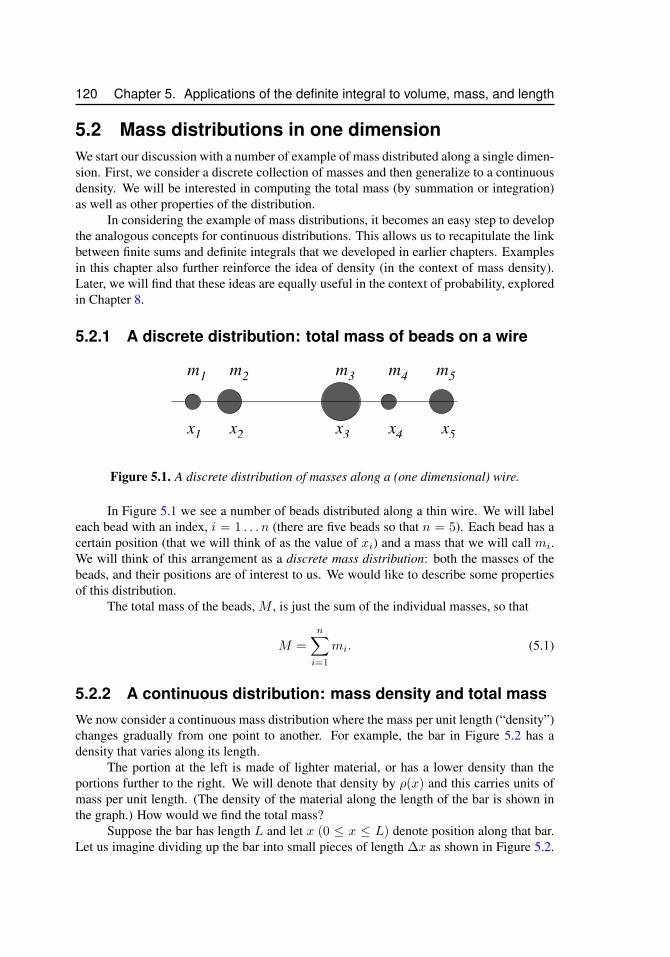
120 Chapter 5. Applications of the definite integral to volume, mass, and length
5.2 Mass distributions in one dimensionWe start our discussion with a number of example of mass distributed along a single dimen-sion. First, we consider a discrete collection of masses and then generalize to a continuousdensity. We will be interested in computing the total mass (by summation or integration)as well as other properties of the distribution.
In considering the example of mass distributions, it becomes an easy step to developthe analogous concepts for continuous distributions. This allows us to recapitulate the linkbetween finite sums and definite integrals that we developed in earlier chapters. Examplesin this chapter also further reinforce the idea of density (in the context of mass density).Later, we will find that these ideas are equally useful in the context of probability, exploredin Chapter 8.
5.2.1 A discrete distribution: total mass of beads on a wire
5
m1
m2
m3
m4
m5
x1
x2
x3
x4
x
Figure 5.1. A discrete distribution of masses along a (one dimensional) wire.
In Figure 5.1 we see a number of beads distributed along a thin wire. We will labeleach bead with an index, i = 1 . . . n (there are five beads so that n = 5). Each bead has acertain position (that we will think of as the value of xi) and a mass that we will call mi.We will think of this arrangement as a discrete mass distribution: both the masses of thebeads, and their positions are of interest to us. We would like to describe some propertiesof this distribution.
The total mass of the beads, M , is just the sum of the individual masses, so that
M =
n∑i=1
mi. (5.1)
5.2.2 A continuous distribution: mass density and total massWe now consider a continuous mass distribution where the mass per unit length (“density”)changes gradually from one point to another. For example, the bar in Figure 5.2 has adensity that varies along its length.
The portion at the left is made of lighter material, or has a lower density than theportions further to the right. We will denote that density by ρ(x) and this carries units ofmass per unit length. (The density of the material along the length of the bar is shown inthe graph.) How would we find the total mass?
Suppose the bar has length L and let x (0 ≤ x ≤ L) denote position along that bar.Let us imagine dividing up the bar into small pieces of length ∆x as shown in Figure 5.2.
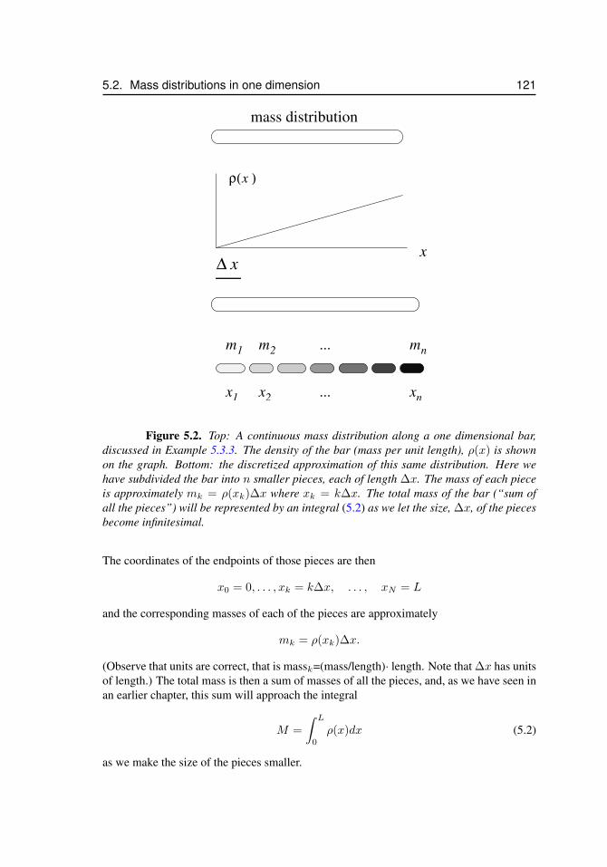
5.2. Mass distributions in one dimension 121
x
mass distribution
ρ( )x
...
∆ x
m1
m2
mn
x1
x2
xn
...
Figure 5.2. Top: A continuous mass distribution along a one dimensional bar,discussed in Example 5.3.3. The density of the bar (mass per unit length), ρ(x) is shownon the graph. Bottom: the discretized approximation of this same distribution. Here wehave subdivided the bar into n smaller pieces, each of length ∆x. The mass of each pieceis approximately mk = ρ(xk)∆x where xk = k∆x. The total mass of the bar (“sum ofall the pieces”) will be represented by an integral (5.2) as we let the size, ∆x, of the piecesbecome infinitesimal.
The coordinates of the endpoints of those pieces are then
x0 = 0, . . . , xk = k∆x, . . . , xN = L
and the corresponding masses of each of the pieces are approximately
mk = ρ(xk)∆x.
(Observe that units are correct, that is massk=(mass/length)· length. Note that ∆x has unitsof length.) The total mass is then a sum of masses of all the pieces, and, as we have seen inan earlier chapter, this sum will approach the integral
M =
∫ L
0
ρ(x)dx (5.2)
as we make the size of the pieces smaller.
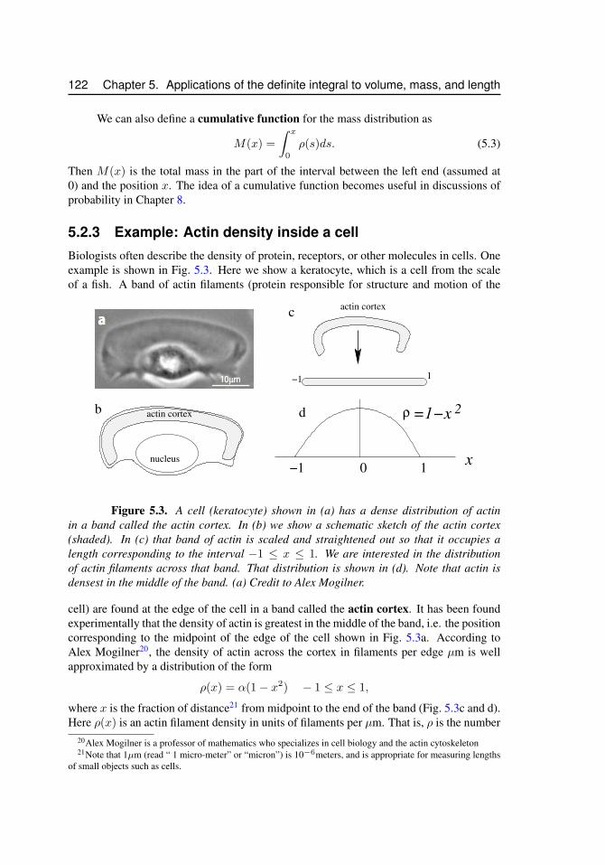
122 Chapter 5. Applications of the definite integral to volume, mass, and length
We can also define a cumulative function for the mass distribution as
M(x) =
∫ x
0
ρ(s)ds. (5.3)
Then M(x) is the total mass in the part of the interval between the left end (assumed at0) and the position x. The idea of a cumulative function becomes useful in discussions ofprobability in Chapter 8.
5.2.3 Example: Actin density inside a cellBiologists often describe the density of protein, receptors, or other molecules in cells. Oneexample is shown in Fig. 5.3. Here we show a keratocyte, which is a cell from the scaleof a fish. A band of actin filaments (protein responsible for structure and motion of the
2
nucleus
actin cortex
actin cortex
b
c
d
−11
−1 0 1x
=1−xρ
Figure 5.3. A cell (keratocyte) shown in (a) has a dense distribution of actinin a band called the actin cortex. In (b) we show a schematic sketch of the actin cortex(shaded). In (c) that band of actin is scaled and straightened out so that it occupies alength corresponding to the interval −1 ≤ x ≤ 1. We are interested in the distributionof actin filaments across that band. That distribution is shown in (d). Note that actin isdensest in the middle of the band. (a) Credit to Alex Mogilner.
cell) are found at the edge of the cell in a band called the actin cortex. It has been foundexperimentally that the density of actin is greatest in the middle of the band, i.e. the positioncorresponding to the midpoint of the edge of the cell shown in Fig. 5.3a. According toAlex Mogilner20, the density of actin across the cortex in filaments per edge µm is wellapproximated by a distribution of the form
ρ(x) = α(1− x2) − 1 ≤ x ≤ 1,
where x is the fraction of distance21 from midpoint to the end of the band (Fig. 5.3c and d).Here ρ(x) is an actin filament density in units of filaments per µm. That is, ρ is the number
20Alex Mogilner is a professor of mathematics who specializes in cell biology and the actin cytoskeleton21Note that 1µm (read “ 1 micro-meter” or “micron”) is 10−6meters, and is appropriate for measuring lengths
of small objects such as cells.
5.3. Mass distribution and the center of mass 123
of actin fibers per unit length.We can find the total number of actin filaments, N in the band by integration, i.e.
N =
∫ 1
−1
α(1− x2) dx = α
∫ 1
−1
(1− x2) dx.
The integral above has already been computed (Integral 2.) in the Examples 3.6.2 of Chap-ter 3 and was found to be 4/3. Thus, we have that there are N = 4α/3 actin filaments inthe band.
5.3 Mass distribution and the center of massIt is useful to describe several other properties of mass distributions. We first define the“center of mass”, x which is akin to an average x coordinate.
5.3.1 Center of mass of a discrete distributionThe center of mass x of a mass distribution is given by:
x =1
M
n∑i=1
ximi .
This can also be written in the form
x =
∑ni=1 ximi∑ni=1mi
.
5.3.2 Center of mass of a continuous distributionWe can generalize the concept of the center of mass for a continuous mass density. Ourusual approach of subdividing the interval 0 ≤ x ≤ L and computing a Riemann sum leadsto
x =1
M
n∑i=1
xiρ(xi)∆x.
As ∆x → dx, this becomes an integral. Based on this, it makes sense to define the centerof mass of the continuous mass distribution as follows:
x =1
M
∫ L
0
xρ(x)dx .
We can also write this in the form
x =
∫ L0xρ(x)dx∫ L
0ρ(x)dx
.
124 Chapter 5. Applications of the definite integral to volume, mass, and length
5.3.3 Example: Center of mass vs average mass densityHere we distinguish between two (potentially confusing) quantities in the context of anexample.
A long thin bar of length L is made of material whose density varies along the lengthof the bar. Let x be distance from one end of the bar. Suppose that the mass density is givenby
ρ(x) = ax, 0 ≤ x ≤ L.
This type of mass density is shown in a panel in Fig. 5.2.
(a) Find the total mass of the bar.
(b) Find the average mass density along the bar.
(c) Find the center of mass of the bar.
(d) Where along the length of the bar should you cut to get two pieces of equal mass?
Solution
(a) From our previous discussion, the total mass of the bar is
M =
∫ L
0
ax dx =ax2
2
∣∣∣∣L0
=aL2
2.
(b) The average mass density along the bar is computed just as one would compute theaverage value of a function: integrate the function over an interval and divide by thelength of the interval. An example of this type appeared in Section 4.5. Thus
ρ =1
L
∫ L
0
ρ(x) dx =1
L
(aL2
2
)=aL
2
A bar having a uniform density ρ = aL/2 would have the same total mass as the barin this example. (This is the physical interpretation of average mass density.)
(c) The center of mass of the bar is
x =
∫ L0xp(x) dx
M=
1
M
∫ L
0
ax2 dx =a
M
x3
3
∣∣∣∣L0
=2a
aL2
L3
3=
2
3L.
Observe that the center of mass is an “average x coordinate”, which is not the same asthe average mass density.
(d) We can use the cumulative function defined in Eqn. (5.3) to figure out where half of themass is concentrated. Suppose we cut the bar at some position x = s. Then the massof this part of the bar is
M1 =
∫ s
0
ρ(x) dx =as2
2,
5.4. Miscellaneous examples and related problems 125
We ask for what values of s is it true that M1 is exactly half the total mass? Using theresult of part (a), we find that for this to be true, we must have
M1 =M
2, ⇒ as2
2=
1
2
aL2
2
Solving for s leads to
s =1√2L =
√2
2L.
Thus, cutting the bar at a distance (√
2/2)L from x = 0 results in two equal masses.
Remark: the position that subdivides the mass into two equal pieces is analogous tothe idea of a median. This concept will appear again in the context of probability inChapter 8.
5.4 Miscellaneous examples and related problemsThe idea of mass density can be extended to related problems of various kinds. We givesome examples in this section.
Up to now, we have seen examples of mass distributed in one dimension: beads on awire, actin density along the edge of a cell, (in Chapter 4), or a bar of varying density. Forthe continuous distributions, we determined the total mass by integration. Underlying theintegral we computed was the idea that the interval could be “dissected” into small parts(of width ∆x), and a sum of pieces transformed into an integral. In the next examples, weconsider similar ideas, but instead of dissecting the region into 1-dimensional intervals, wehave slightly more interesting geometries.
5.4.1 Example: A glucose density gradientA cylindrical test-tube of radius r, and height h, contains a solution of glucose which hasbeen prepared so that the concentration of glucose is greatest at the bottom and decreasesgradually towards the top of the tube. (This is called a density gradient). Suppose that theconcentration c as a function of the depth x is c(x) = 0.1 + 0.5x grams per centimeter3.(x = 0 at the top of the tube, and x = h at the bottom of the tube.) In Figure 5.4 we show aschematic version of what this gradient might look like. (In reality, the transition betweenhigh and low concentration would be smoother than shown in this figure.) Determine thetotal amount of glucose in the tube (in gm). Neglect the “rounded” lower portion of thetube: i.e. assume that it is a simple cylinder.
Solution
We assume a simple cylindrical tube and consider imaginary “slices” of this tube alongits vertical axis, here labeled as the “x” axis. Suppose that the thickness of a slice is ∆x.Then the volume of each of these (disk shaped) slices is πr2∆x. The amount of glucose inthe slice is approximately equal to the concentration c(x) multiplied by the volume of theslice, i.e. the small slice contains an amount πr2∆xc(x) of glucose. In order to sum up the
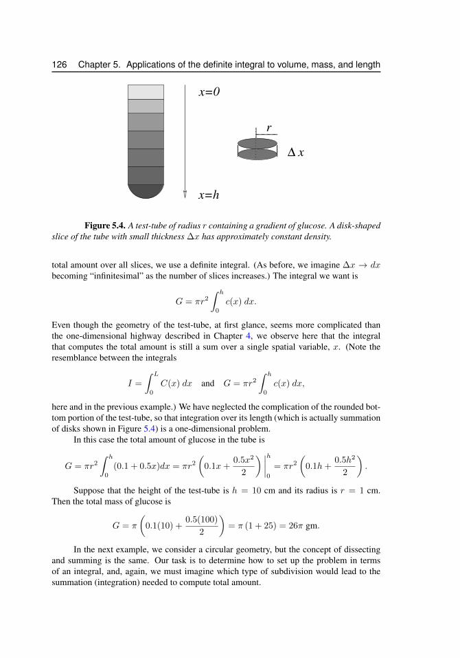
126 Chapter 5. Applications of the definite integral to volume, mass, and length
x=0
r
x=h
∆ x
Figure 5.4. A test-tube of radius r containing a gradient of glucose. A disk-shapedslice of the tube with small thickness ∆x has approximately constant density.
total amount over all slices, we use a definite integral. (As before, we imagine ∆x → dxbecoming “infinitesimal” as the number of slices increases.) The integral we want is
G = πr2
∫ h
0
c(x) dx.
Even though the geometry of the test-tube, at first glance, seems more complicated thanthe one-dimensional highway described in Chapter 4, we observe here that the integralthat computes the total amount is still a sum over a single spatial variable, x. (Note theresemblance between the integrals
I =
∫ L
0
C(x) dx and G = πr2
∫ h
0
c(x) dx,
here and in the previous example.) We have neglected the complication of the rounded bot-tom portion of the test-tube, so that integration over its length (which is actually summationof disks shown in Figure 5.4) is a one-dimensional problem.
In this case the total amount of glucose in the tube is
G = πr2
∫ h
0
(0.1 + 0.5x)dx = πr2
(0.1x+
0.5x2
2
) ∣∣∣∣h0
= πr2
(0.1h+
0.5h2
2
).
Suppose that the height of the test-tube is h = 10 cm and its radius is r = 1 cm.Then the total mass of glucose is
G = π
(0.1(10) +
0.5(100)
2
)= π (1 + 25) = 26π gm.
In the next example, we consider a circular geometry, but the concept of dissectingand summing is the same. Our task is to determine how to set up the problem in termsof an integral, and, again, we must imagine which type of subdivision would lead to thesummation (integration) needed to compute total amount.
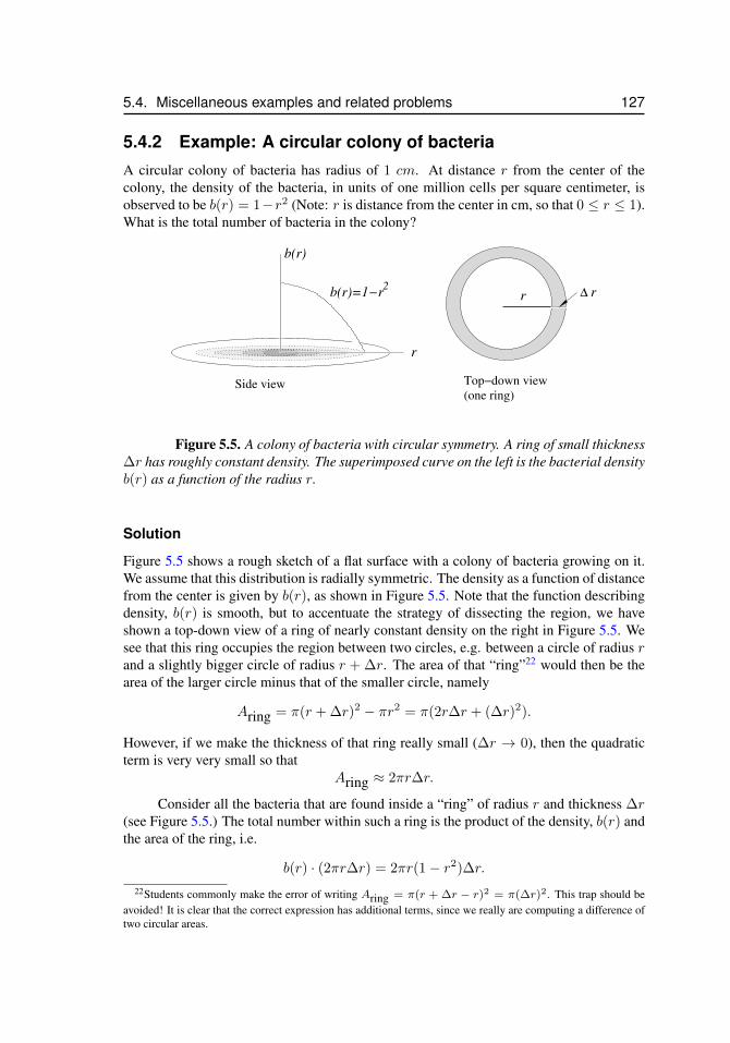
5.4. Miscellaneous examples and related problems 127
5.4.2 Example: A circular colony of bacteriaA circular colony of bacteria has radius of 1 cm. At distance r from the center of thecolony, the density of the bacteria, in units of one million cells per square centimeter, isobserved to be b(r) = 1−r2 (Note: r is distance from the center in cm, so that 0 ≤ r ≤ 1).What is the total number of bacteria in the colony?
(one ring)
∆ r
Side view Top−down view
r
b(r)
b(r)=1−r
r
2
Figure 5.5. A colony of bacteria with circular symmetry. A ring of small thickness∆r has roughly constant density. The superimposed curve on the left is the bacterial densityb(r) as a function of the radius r.
Solution
Figure 5.5 shows a rough sketch of a flat surface with a colony of bacteria growing on it.We assume that this distribution is radially symmetric. The density as a function of distancefrom the center is given by b(r), as shown in Figure 5.5. Note that the function describingdensity, b(r) is smooth, but to accentuate the strategy of dissecting the region, we haveshown a top-down view of a ring of nearly constant density on the right in Figure 5.5. Wesee that this ring occupies the region between two circles, e.g. between a circle of radius rand a slightly bigger circle of radius r + ∆r. The area of that “ring”22 would then be thearea of the larger circle minus that of the smaller circle, namely
Aring = π(r + ∆r)2 − πr2 = π(2r∆r + (∆r)2).
However, if we make the thickness of that ring really small (∆r → 0), then the quadraticterm is very very small so that
Aring ≈ 2πr∆r.
Consider all the bacteria that are found inside a “ring” of radius r and thickness ∆r(see Figure 5.5.) The total number within such a ring is the product of the density, b(r) andthe area of the ring, i.e.
b(r) · (2πr∆r) = 2πr(1− r2)∆r.
22Students commonly make the error of writing Aring = π(r + ∆r − r)2 = π(∆r)2. This trap should beavoided! It is clear that the correct expression has additional terms, since we really are computing a difference oftwo circular areas.
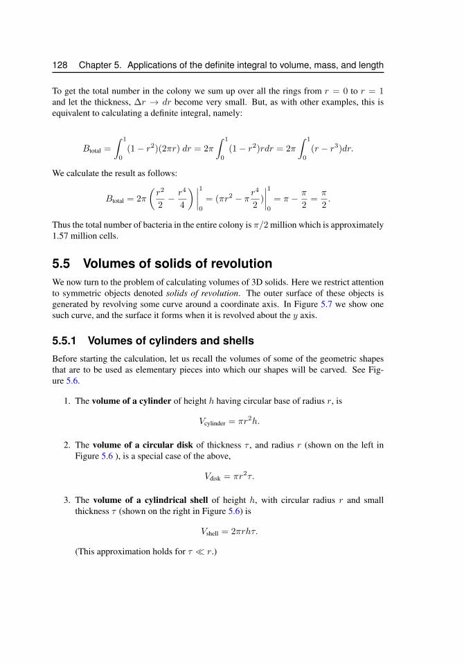
128 Chapter 5. Applications of the definite integral to volume, mass, and length
To get the total number in the colony we sum up over all the rings from r = 0 to r = 1and let the thickness, ∆r → dr become very small. But, as with other examples, this isequivalent to calculating a definite integral, namely:
Btotal =
∫ 1
0
(1− r2)(2πr) dr = 2π
∫ 1
0
(1− r2)rdr = 2π
∫ 1
0
(r − r3)dr.
We calculate the result as follows:
Btotal = 2π
(r2
2− r4
4
) ∣∣∣∣10
= (πr2 − π r4
2)
∣∣∣∣10
= π − π
2=π
2.
Thus the total number of bacteria in the entire colony is π/2 million which is approximately1.57 million cells.
5.5 Volumes of solids of revolutionWe now turn to the problem of calculating volumes of 3D solids. Here we restrict attentionto symmetric objects denoted solids of revolution. The outer surface of these objects isgenerated by revolving some curve around a coordinate axis. In Figure 5.7 we show onesuch curve, and the surface it forms when it is revolved about the y axis.
5.5.1 Volumes of cylinders and shellsBefore starting the calculation, let us recall the volumes of some of the geometric shapesthat are to be used as elementary pieces into which our shapes will be carved. See Fig-ure 5.6.
1. The volume of a cylinder of height h having circular base of radius r, is
Vcylinder = πr2h.
2. The volume of a circular disk of thickness τ , and radius r (shown on the left inFigure 5.6 ), is a special case of the above,
Vdisk = πr2τ.
3. The volume of a cylindrical shell of height h, with circular radius r and smallthickness τ (shown on the right in Figure 5.6) is
Vshell = 2πrhτ.
(This approximation holds for τ � r.)
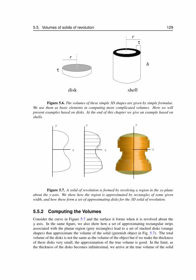
5.5. Volumes of solids of revolution 129
r
h
τ
r
τ
disk shell
Figure 5.6. The volumes of these simple 3D shapes are given by simple formulae.We use them as basic elements in computing more complicated volumes. Here we willpresent examples based on disks. At the end of this chapter we give an example based onshells.
y
x x x
y y
Figure 5.7. A solid of revolution is formed by revolving a region in the xy-planeabout the y-axis. We show how the region is approximated by rectangles of some givenwidth, and how these form a set of approximating disks for the 3D solid of revolution.
5.5.2 Computing the VolumesConsider the curve in Figure 5.7 and the surface it forms when it is revolved about they axis. In the same figure, we also show how a set of approximating rectangular stripsassociated with the planar region (grey rectangles) lead to a set of stacked disks (orangeshapes) that approximate the volume of the solid (greenish object in Fig. 5.7). The totalvolume of the disks is not the same as the volume of the object but if we make the thicknessof these disks very small, the approximation of the true volume is good. In the limit, asthe thickness of the disks becomes infinitesimal, we arrive at the true volume of the solid
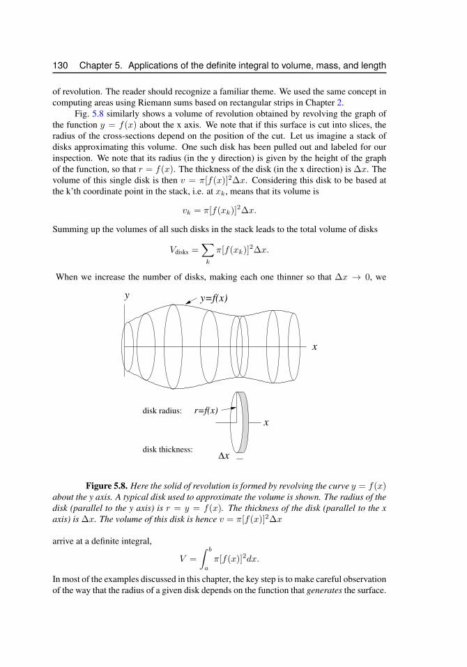
130 Chapter 5. Applications of the definite integral to volume, mass, and length
of revolution. The reader should recognize a familiar theme. We used the same concept incomputing areas using Riemann sums based on rectangular strips in Chapter 2.
Fig. 5.8 similarly shows a volume of revolution obtained by revolving the graph ofthe function y = f(x) about the x axis. We note that if this surface is cut into slices, theradius of the cross-sections depend on the position of the cut. Let us imagine a stack ofdisks approximating this volume. One such disk has been pulled out and labeled for ourinspection. We note that its radius (in the y direction) is given by the height of the graphof the function, so that r = f(x). The thickness of the disk (in the x direction) is ∆x. Thevolume of this single disk is then v = π[f(x)]2∆x. Considering this disk to be based atthe k’th coordinate point in the stack, i.e. at xk, means that its volume is
vk = π[f(xk)]2∆x.
Summing up the volumes of all such disks in the stack leads to the total volume of disks
Vdisks =∑k
π[f(xk)]2∆x.
When we increase the number of disks, making each one thinner so that ∆x → 0, we
disk thickness:
disk radius:
x∆
x
y
x
y=f(x)
r=f(x)
Figure 5.8. Here the solid of revolution is formed by revolving the curve y = f(x)about the y axis. A typical disk used to approximate the volume is shown. The radius of thedisk (parallel to the y axis) is r = y = f(x). The thickness of the disk (parallel to the xaxis) is ∆x. The volume of this disk is hence v = π[f(x)]2∆x
arrive at a definite integral,
V =
∫ b
a
π[f(x)]2dx.
In most of the examples discussed in this chapter, the key step is to make careful observationof the way that the radius of a given disk depends on the function that generates the surface.
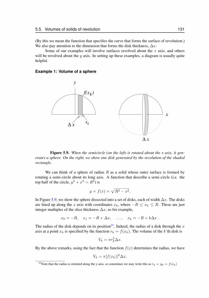
5.5. Volumes of solids of revolution 131
(By this we mean the function that specifies the curve that forms the surface of revolution.)We also pay attention to the dimension that forms the disk thickness, ∆x.
Some of our examples will involve surfaces revolved about the x axis, and otherswill be revolved about the y axis. In setting up these examples, a diagram is usually quitehelpful.
Example 1: Volume of a sphere
k
y
x
f(x )k
∆ x
∆ xx
Figure 5.9. When the semicircle (on the left) is rotated about the x axis, it gen-erates a sphere. On the right, we show one disk generated by the revolution of the shadedrectangle.
We can think of a sphere of radius R as a solid whose outer surface is formed byrotating a semi-circle about its long axis. A function that describe a semi-circle (i.e. thetop half of the circle, y2 + x2 = R2) is
y = f(x) =√R2 − x2.
In Figure 5.9, we show the sphere dissected into a set of disks, each of width ∆x. The disksare lined up along the x axis with coordinates xk, where −R ≤ xk ≤ R. These are justinteger multiples of the slice thickness ∆x, so for example,
x0 = −R, x1 = −R+ ∆x, . . . , xk = −R+ k∆x .
The radius of the disk depends on its position23. Indeed, the radius of a disk through the xaxis at a point xk is specified by the function rk = f(xk). The volume of the k’th disk is
Vk = πr2k∆x.
By the above remarks, using the fact that the function f(x) determines the radius, we have
Vk = π[f(xk)]2∆x,
23Note that the radius is oriented along the y axis, so sometimes we may write this as rk = yk = f(xk)
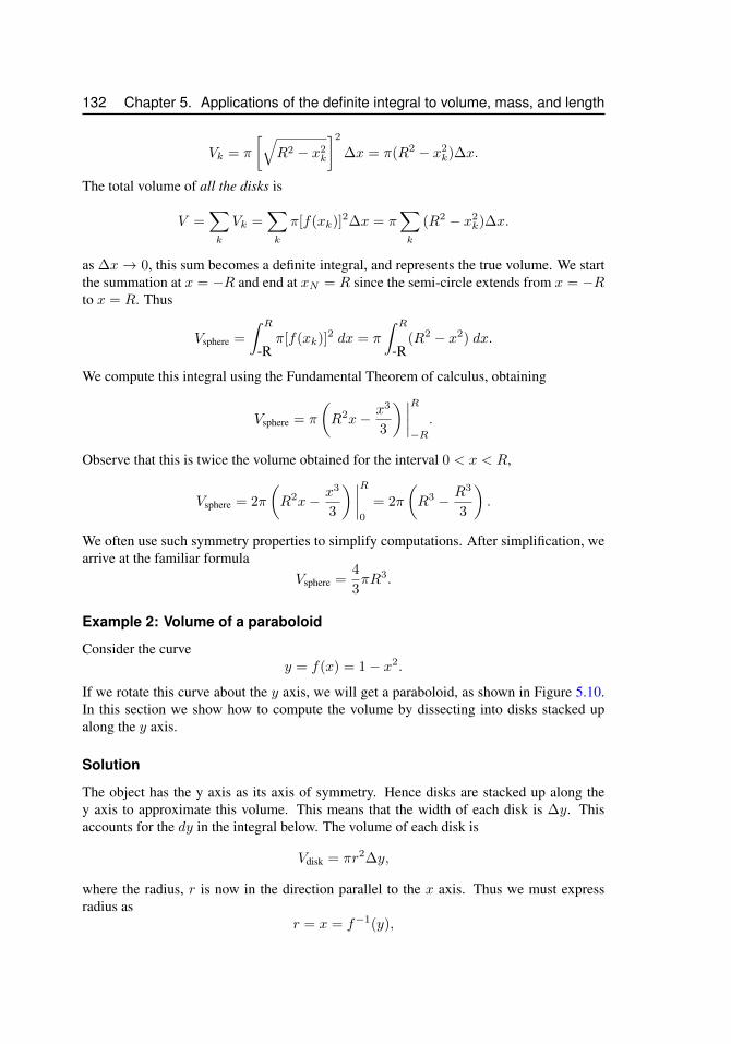
132 Chapter 5. Applications of the definite integral to volume, mass, and length
Vk = π
[√R2 − x2
k
]2
∆x = π(R2 − x2k)∆x.
The total volume of all the disks is
V =∑k
Vk =∑k
π[f(xk)]2∆x = π∑k
(R2 − x2k)∆x.
as ∆x→ 0, this sum becomes a definite integral, and represents the true volume. We startthe summation at x = −R and end at xN = R since the semi-circle extends from x = −Rto x = R. Thus
Vsphere =
∫ R
-Rπ[f(xk)]2 dx = π
∫ R
-R(R2 − x2) dx.
We compute this integral using the Fundamental Theorem of calculus, obtaining
Vsphere = π
(R2x− x3
3
) ∣∣∣∣R−R.
Observe that this is twice the volume obtained for the interval 0 < x < R,
Vsphere = 2π
(R2x− x3
3
) ∣∣∣∣R0
= 2π
(R3 − R3
3
).
We often use such symmetry properties to simplify computations. After simplification, wearrive at the familiar formula
Vsphere =4
3πR3.
Example 2: Volume of a paraboloid
Consider the curvey = f(x) = 1− x2.
If we rotate this curve about the y axis, we will get a paraboloid, as shown in Figure 5.10.In this section we show how to compute the volume by dissecting into disks stacked upalong the y axis.
Solution
The object has the y axis as its axis of symmetry. Hence disks are stacked up along they axis to approximate this volume. This means that the width of each disk is ∆y. Thisaccounts for the dy in the integral below. The volume of each disk is
Vdisk = πr2∆y,
where the radius, r is now in the direction parallel to the x axis. Thus we must expressradius as
r = x = f−1(y),
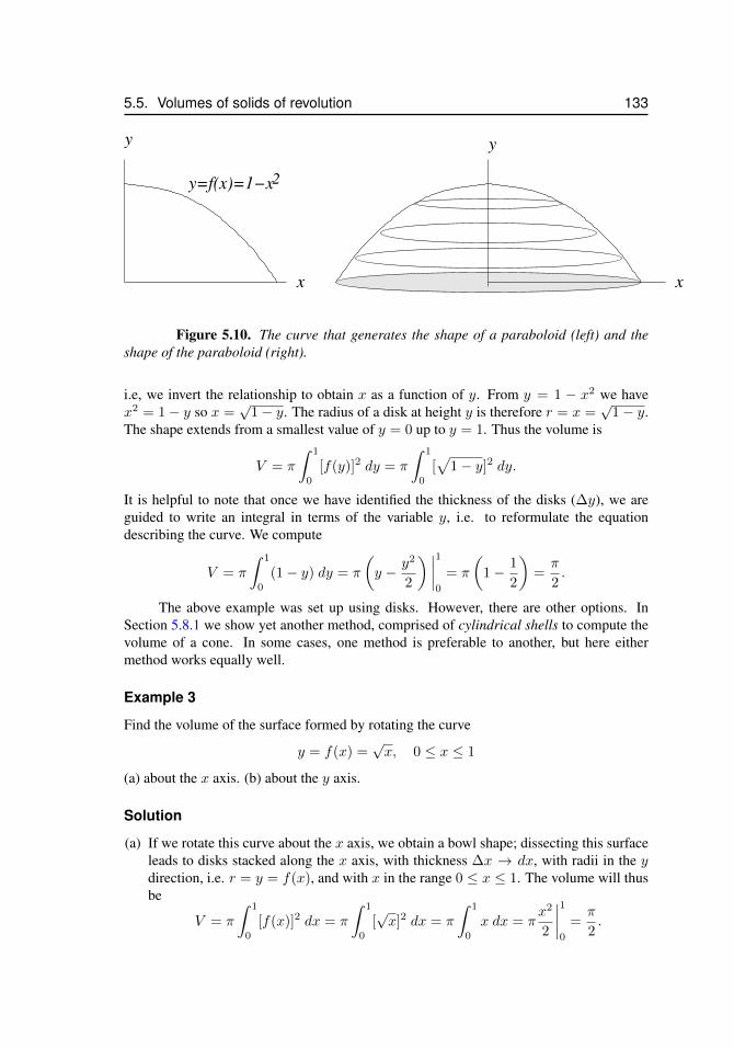
5.5. Volumes of solids of revolution 133
2
y
x x
y
y=f(x)=1−x
Figure 5.10. The curve that generates the shape of a paraboloid (left) and theshape of the paraboloid (right).
i.e, we invert the relationship to obtain x as a function of y. From y = 1 − x2 we havex2 = 1− y so x =
√1− y. The radius of a disk at height y is therefore r = x =
√1− y.
The shape extends from a smallest value of y = 0 up to y = 1. Thus the volume is
V = π
∫ 1
0
[f(y)]2 dy = π
∫ 1
0
[√
1− y]2 dy.
It is helpful to note that once we have identified the thickness of the disks (∆y), we areguided to write an integral in terms of the variable y, i.e. to reformulate the equationdescribing the curve. We compute
V = π
∫ 1
0
(1− y) dy = π
(y − y2
2
) ∣∣∣∣10
= π
(1− 1
2
)=π
2.
The above example was set up using disks. However, there are other options. InSection 5.8.1 we show yet another method, comprised of cylindrical shells to compute thevolume of a cone. In some cases, one method is preferable to another, but here eithermethod works equally well.
Example 3
Find the volume of the surface formed by rotating the curve
y = f(x) =√x, 0 ≤ x ≤ 1
(a) about the x axis. (b) about the y axis.
Solution
(a) If we rotate this curve about the x axis, we obtain a bowl shape; dissecting this surfaceleads to disks stacked along the x axis, with thickness ∆x → dx, with radii in the ydirection, i.e. r = y = f(x), and with x in the range 0 ≤ x ≤ 1. The volume will thusbe
V = π
∫ 1
0
[f(x)]2 dx = π
∫ 1
0
[√x]2 dx = π
∫ 1
0
x dx = πx2
2
∣∣∣∣10
=π
2.
134 Chapter 5. Applications of the definite integral to volume, mass, and length
(b) When the curve is rotated about the y axis, it forms a surface with a sharp point at theorigin. The disks are stacked along the y axis, with thickness ∆y → dy, and radii inthe x direction. We must rewrite the function in the form
x = g(y) = y2.
We now use the interval along the y axis, i.e. 0 < y < 1 The volume is then
V = π
∫ 1
0
[f(y)]2 dy = π
∫ 1
0
[y2]2 dy = π
∫ 1
0
y4 dy = πy5
5
∣∣∣∣10
=π
5.
5.6 Length of a curve: Arc lengthAnalytic geometry provides a simple way to compute the length of a straight line segment,based on the distance formula24. Recall that, given points P1 = (x1, y1) and P2 = (x2, y2),the length of the line joining those points is
d =√
(x2 − x1)2 + (y2 − y1)2.
Things are more complicated for “curves” that are not straight lines, but in many cases, weare interested in calculating the length of such curves. In this section we describe how thiscan be done using the definite integral “technology”.
The idea of dissection also applies to the problem of determining the length of acurve. In Figure 5.11, we see the general idea of subdividing a curve into many small“arcs”. Before we look in detail at this construction, we consider a simple example, shownin Figure 5.12. In the triangle shown, by the Pythagorean theorem we have the length ofthe sloped side related as follows to the side lengths ∆x,∆y:
∆`2 = ∆x2 + ∆y2,
∆` =√
∆x2 + ∆y2 =
(√1 +
∆y2
∆x2
)∆x =
√1 +
(∆y
∆x
)2
∆x.
We now consider a curve given by some function
y = f(x) a < x < b,
as shown in Figure 5.11(a). We will approximate this curve by a set of line segments, asshown in Figure 5.11(b). To obtain these, we have selected some step size ∆x along thex axis, and placed points on the curve at each of these x values. We connect the pointswith straight line segments, and determine the lengths of those segments. (The total lengthof the segments is only an approximation of the length of the curve, but as the subdivisiongets finer and finer, we will arrive at the true total length of the curve.)
We show one such segment enlarged in the circular inset in Figure 5.11. Its slope,shown at right is given by ∆y/∆x. According to our remarks, above, the length of thissegment is given by
∆` =
√1 +
(∆y
∆x
)2
∆x.
24The reader should recall that this formula is a simple application of Pythagorean theorem.
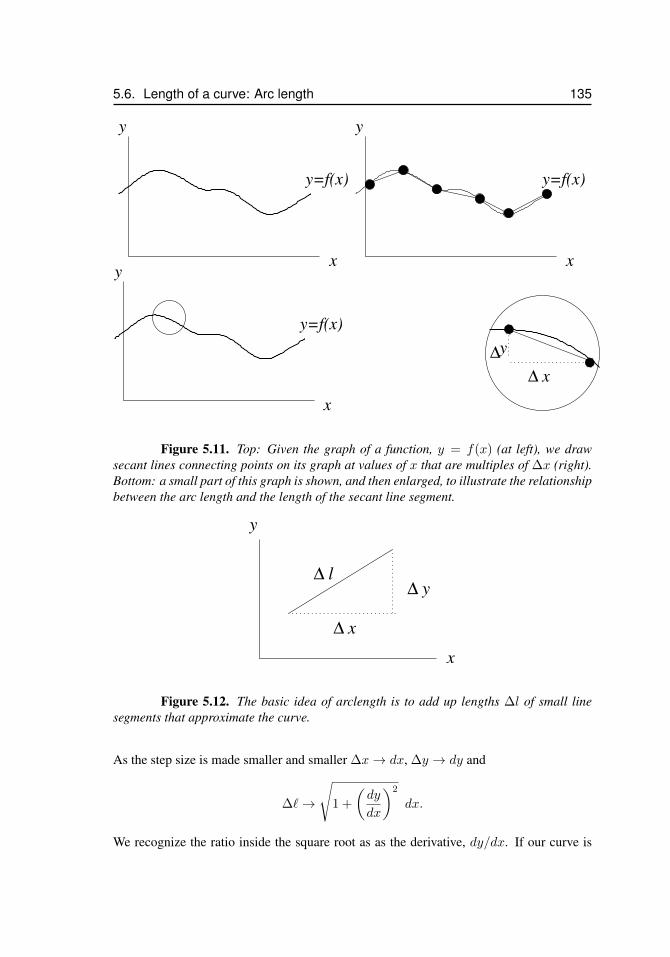
5.6. Length of a curve: Arc length 135
x
y
y=f(x)
x
y
y=f(x)
x
y
y=f(x)
x
y
∆
∆
Figure 5.11. Top: Given the graph of a function, y = f(x) (at left), we drawsecant lines connecting points on its graph at values of x that are multiples of ∆x (right).Bottom: a small part of this graph is shown, and then enlarged, to illustrate the relationshipbetween the arc length and the length of the secant line segment.
y
x
x
y
∆
∆∆ l
Figure 5.12. The basic idea of arclength is to add up lengths ∆l of small linesegments that approximate the curve.
As the step size is made smaller and smaller ∆x→ dx, ∆y → dy and
∆`→
√1 +
(dy
dx
)2
dx.
We recognize the ratio inside the square root as as the derivative, dy/dx. If our curve is
136 Chapter 5. Applications of the definite integral to volume, mass, and length
given by a function y = f(x) then we can rewrite this as
d` =
√1 + (f ′(x))
2dx.
Thus, the length of the entire curve is obtained from summing (i.e. adding up) these smallpieces, i.e.
L =
∫ b
a
√1 + (f ′(x))
2dx. (5.4)
Example 1
Find the length of a line whose slope is−2 given that the line extends from x = 1 to x = 5.
Solution
We could find the equation of the line and use the distance formula. But for the purpose ofthis example, we apply the method of Equation (5.4): we are given that the slope f ′(x) is-2. The integral in question is
L =
∫ 5
1
√1 + (f ′(x))2 dx =
∫ 5
1
√1 + (−2)2 dx =
∫ 1
5
√5 dx.
We get
L =√
5
∫ 5
1
dx =√
5x
∣∣∣∣51
=√
5[5− 1] = 4√
5.
Example 2
Find an integral that represents the length of the curve that forms the graph of the function
y = f(x) = x3, 1 < x < 2.
Solution
We find thatdy
dx= f ′(x) = 3x2.
Thus, the integral is
L =
∫ 2
1
√1 + (3x2)2 dx =
∫ 2
1
√1 + 9x4 dx.
At this point, we will not attempt to find the actual length, as we must first develop tech-niques for finding the anti-derivative for functions such as
√1 + 9x4.
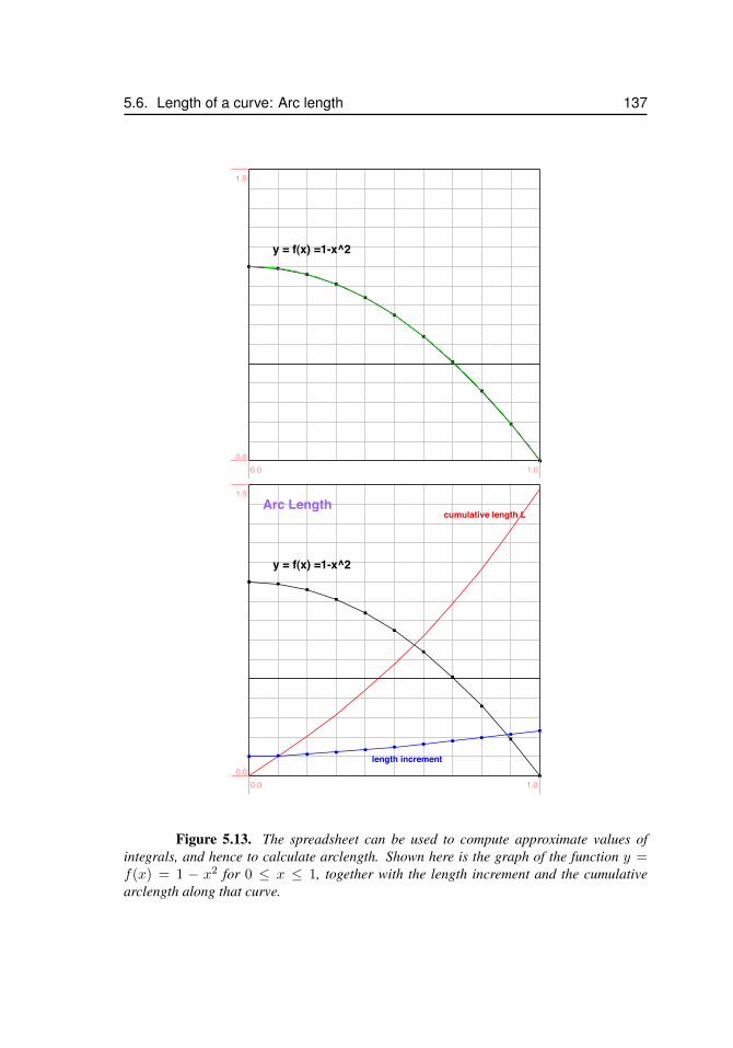
5.6. Length of a curve: Arc length 137
y = f(x) =1-x^2
0.0 1.00.0
1.5
y = f(x) =1-x^2
cumulative length L
length increment
Arc Length
0.0 1.00.0
1.5
Figure 5.13. The spreadsheet can be used to compute approximate values ofintegrals, and hence to calculate arclength. Shown here is the graph of the function y =f(x) = 1 − x2 for 0 ≤ x ≤ 1, together with the length increment and the cumulativearclength along that curve.
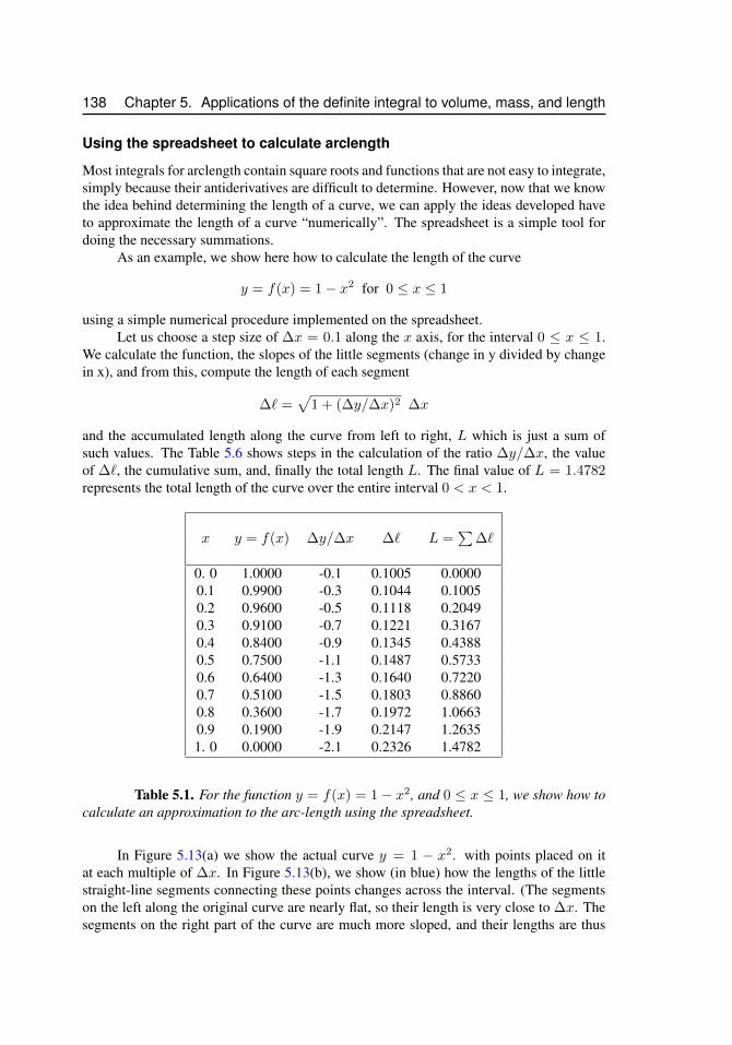
138 Chapter 5. Applications of the definite integral to volume, mass, and length
Using the spreadsheet to calculate arclength
Most integrals for arclength contain square roots and functions that are not easy to integrate,simply because their antiderivatives are difficult to determine. However, now that we knowthe idea behind determining the length of a curve, we can apply the ideas developed haveto approximate the length of a curve “numerically”. The spreadsheet is a simple tool fordoing the necessary summations.
As an example, we show here how to calculate the length of the curve
y = f(x) = 1− x2 for 0 ≤ x ≤ 1
using a simple numerical procedure implemented on the spreadsheet.Let us choose a step size of ∆x = 0.1 along the x axis, for the interval 0 ≤ x ≤ 1.
We calculate the function, the slopes of the little segments (change in y divided by changein x), and from this, compute the length of each segment
∆` =√
1 + (∆y/∆x)2 ∆x
and the accumulated length along the curve from left to right, L which is just a sum ofsuch values. The Table 5.6 shows steps in the calculation of the ratio ∆y/∆x, the valueof ∆`, the cumulative sum, and, finally the total length L. The final value of L = 1.4782represents the total length of the curve over the entire interval 0 < x < 1.
x y = f(x) ∆y/∆x ∆` L =∑
∆`
0. 0 1.0000 -0.1 0.1005 0.00000.1 0.9900 -0.3 0.1044 0.10050.2 0.9600 -0.5 0.1118 0.20490.3 0.9100 -0.7 0.1221 0.31670.4 0.8400 -0.9 0.1345 0.43880.5 0.7500 -1.1 0.1487 0.57330.6 0.6400 -1.3 0.1640 0.72200.7 0.5100 -1.5 0.1803 0.88600.8 0.3600 -1.7 0.1972 1.06630.9 0.1900 -1.9 0.2147 1.26351. 0 0.0000 -2.1 0.2326 1.4782
Table 5.1. For the function y = f(x) = 1− x2, and 0 ≤ x ≤ 1, we show how tocalculate an approximation to the arc-length using the spreadsheet.
In Figure 5.13(a) we show the actual curve y = 1 − x2. with points placed on itat each multiple of ∆x. In Figure 5.13(b), we show (in blue) how the lengths of the littlestraight-line segments connecting these points changes across the interval. (The segmentson the left along the original curve are nearly flat, so their length is very close to ∆x. Thesegments on the right part of the curve are much more sloped, and their lengths are thus
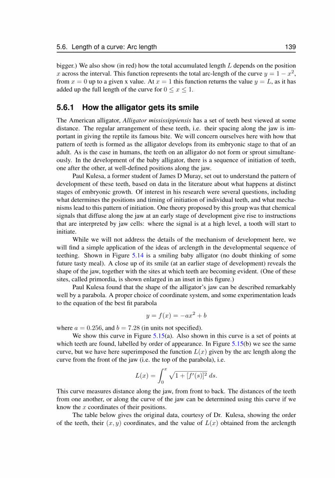
5.6. Length of a curve: Arc length 139
bigger.) We also show (in red) how the total accumulated length L depends on the positionx across the interval. This function represents the total arc-length of the curve y = 1− x2,from x = 0 up to a given x value. At x = 1 this function returns the value y = L, as it hasadded up the full length of the curve for 0 ≤ x ≤ 1.
5.6.1 How the alligator gets its smileThe American alligator, Alligator mississippiensis has a set of teeth best viewed at somedistance. The regular arrangement of these teeth, i.e. their spacing along the jaw is im-portant in giving the reptile its famous bite. We will concern ourselves here with how thatpattern of teeth is formed as the alligator develops from its embryonic stage to that of anadult. As is the case in humans, the teeth on an alligator do not form or sprout simultane-ously. In the development of the baby alligator, there is a sequence of initiation of teeth,one after the other, at well-defined positions along the jaw.
Paul Kulesa, a former student of James D Muray, set out to understand the pattern ofdevelopment of these teeth, based on data in the literature about what happens at distinctstages of embryonic growth. Of interest in his research were several questions, includingwhat determines the positions and timing of initiation of individual teeth, and what mecha-nisms lead to this pattern of initiation. One theory proposed by this group was that chemicalsignals that diffuse along the jaw at an early stage of development give rise to instructionsthat are interpreted by jaw cells: where the signal is at a high level, a tooth will start toinitiate.
While we will not address the details of the mechanism of development here, wewill find a simple application of the ideas of arclength in the developmental sequence ofteething. Shown in Figure 5.14 is a smiling baby alligator (no doubt thinking of somefuture tasty meal). A close up of its smile (at an earlier stage of development) reveals theshape of the jaw, together with the sites at which teeth are becoming evident. (One of thesesites, called primordia, is shown enlarged in an inset in this figure.)
Paul Kulesa found that the shape of the alligator’s jaw can be described remarkablywell by a parabola. A proper choice of coordinate system, and some experimentation leadsto the equation of the best fit parabola
y = f(x) = −ax2 + b
where a = 0.256, and b = 7.28 (in units not specified).We show this curve in Figure 5.15(a). Also shown in this curve is a set of points at
which teeth are found, labelled by order of appearance. In Figure 5.15(b) we see the samecurve, but we have here superimposed the function L(x) given by the arc length along thecurve from the front of the jaw (i.e. the top of the parabola), i.e.
L(x) =
∫ x
0
√1 + [f ′(s)]2 ds.
This curve measures distance along the jaw, from front to back. The distances of the teethfrom one another, or along the curve of the jaw can be determined using this curve if weknow the x coordinates of their positions.
The table below gives the original data, courtesy of Dr. Kulesa, showing the orderof the teeth, their (x, y) coordinates, and the value of L(x) obtained from the arclength
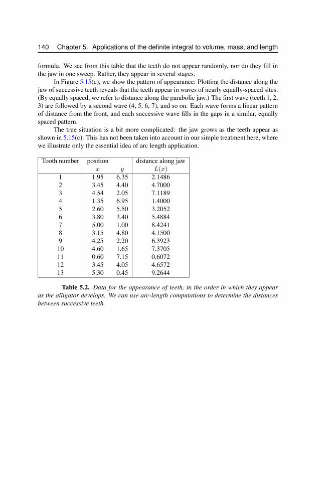
140 Chapter 5. Applications of the definite integral to volume, mass, and length
formula. We see from this table that the teeth do not appear randomly, nor do they fill inthe jaw in one sweep. Rather, they appear in several stages.
In Figure 5.15(c), we show the pattern of appearance: Plotting the distance along thejaw of successive teeth reveals that the teeth appear in waves of nearly equally-spaced sites.(By equally spaced, we refer to distance along the parabolic jaw.) The first wave (teeth 1, 2,3) are followed by a second wave (4, 5, 6, 7), and so on. Each wave forms a linear patternof distance from the front, and each successive wave fills in the gaps in a similar, equallyspaced pattern.
The true situation is a bit more complicated: the jaw grows as the teeth appear asshown in 5.15(c). This has not been taken into account in our simple treatment here, wherewe illustrate only the essential idea of arc length application.
Tooth number position distance along jawx y L(x)
1 1.95 6.35 2.14862 3.45 4.40 4.70003 4.54 2.05 7.11894 1.35 6.95 1.40005 2.60 5.50 3.20526 3.80 3.40 5.48847 5.00 1.00 8.42418 3.15 4.80 4.15009 4.25 2.20 6.3923
10 4.60 1.65 7.370511 0.60 7.15 0.607212 3.45 4.05 4.657213 5.30 0.45 9.2644
Table 5.2. Data for the appearance of teeth, in the order in which they appearas the alligator develops. We can use arc-length computations to determine the distancesbetween successive teeth.
5.6. Length of a curve: Arc length 141
Figure 5.14. Alligator mississippiensis and its teeth

142 Chapter 5. Applications of the definite integral to volume, mass, and length
1
2
3
4
5
6
7
8
9
10
11
12
13
Alligator teeth
-6.0 6.00.0
8.0
jaw y = f(x)
arc length L(x) along jaw
0.0 5.50.0
10.0
(a) (b)
Distance along jaw
1
2
3
4
5
6
7
8
9
10
11
12
13
teeth in order of appearance
0.0 13.00.0
10.0
(c) (d)
Figure 5.15. (a) The parabolic shape of the jaw, showing positions of teeth andnumerical order of emergence. (b) Arc length along the jaw from front to back. (c) Distanceof successive teeth along the jaw. (d) Growth of the jaw.
5.7. Summary 143
5.6.2 References1. P.M. Kulesa and J.D. Murray (1995). Modelling the Wave-like Initiation of Teeth
Primordia in the Alligator. FORMA. Cover Article. Vol. 10, No. 3, 259-280.
2. J.D. Murray and P.M. Kulesa (1996). On A Dynamic Reaction-Diffusion Mechanismfor the Spatial Patterning of Teeth Primordia in the Alligator. Journal of ChemicalPhysics. J. Chem. Soc., Faraday Trans., 92 (16), 2927-2932.
3. P.M. Kulesa, G.C. Cruywagen, S.R. Lubkin, M.W.J. Ferguson and J.D. Murray (1996).Modelling the Spatial Patterning of Teeth Primordia in the Alligator. Acta Biotheo-retica, 44, 153-164.
5.7 SummaryHere are the main points of the chapter:
1. We introduced the idea of a spatially distributed mass density ρ(x) in Section 5.2.2.Here the definite integral represents∫ b
a
ρ(x) dx = Total mass in the interval a ≤ x ≤ b.
2. In this chapter, we defined the center of mass of a (discrete) distribution of n massesby
X =1
M
n∑i=0
ximi. (5.5)
We developed the analogue of this for a continuous mass distribution (distributed inthe interval 0 ≤ x ≤ L). We defined the center of mass of a continuous distributionby the definite integral
x =1
M
∫ L
0
xρ(x)dx . (5.6)
Importantly, the quantities mi in the sum (5.5) carry units of mass, whereas theanalogous quantities in (5.6) are ρ(x)dx. [Recall that ρ(x) is a mass per unit lengthin the case of mass distributed along a bar or straight line.]
3. We defined a cumulative function. In the discrete case, this was defined as In thecontinuous case, it is
M(x) =
∫ x
0
ρ(s)ds.
4. The mean is an average x coordinate, whereas the median is the x coordinate thatsplits the distribution into two equal masses (Geometrically, the median subdividesthe graph of the distribution into two regions of equal areas). The mean and medianare the same only in symmetric distributions. They differ for any distribution that isasymmetric. The mean (but not the median) is influenced more strongly by distantportions of the distribution.
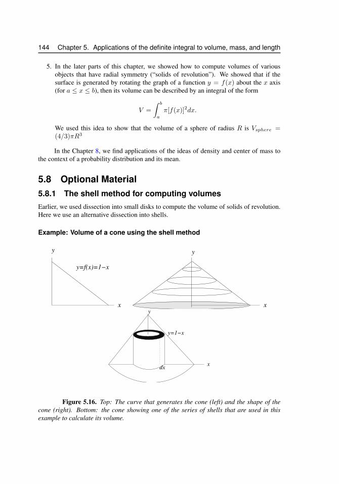
144 Chapter 5. Applications of the definite integral to volume, mass, and length
5. In the later parts of this chapter, we showed how to compute volumes of variousobjects that have radial symmetry (“solids of revolution”). We showed that if thesurface is generated by rotating the graph of a function y = f(x) about the x axis(for a ≤ x ≤ b), then its volume can be described by an integral of the form
V =
∫ b
a
π[f(x)]2dx.
We used this idea to show that the volume of a sphere of radius R is Vsphere =(4/3)πR3
In the Chapter 8, we find applications of the ideas of density and center of mass tothe context of a probability distribution and its mean.
5.8 Optional Material5.8.1 The shell method for computing volumesEarlier, we used dissection into small disks to compute the volume of solids of revolution.Here we use an alternative dissection into shells.
Example: Volume of a cone using the shell method
x
y
y=f(x)=1−x
y
x
x
y
y=1−x
dx
Figure 5.16. Top: The curve that generates the cone (left) and the shape of thecone (right). Bottom: the cone showing one of the series of shells that are used in thisexample to calculate its volume.

5.8. Optional Material 145
We use the shell method to find the volume of the cone formed by rotating the curve
y = 1− x
about the y axis.
Solution
We show the cone and its generating curve in Figure 5.16, together with a representativeshell used in the calculation of total volume. The volume of a cylindrical shell of radius r,height h and thickness τ is
Vshell = 2πrhτ.
We will place these shells one inside the other so that their radii are parallel to the x axis(so r = x). The heights of the shells are determined by their y value (i.e. h = y = 1−x =1− r). For the tallest shell r = 0, and for the flattest shell r = 1. The thickness of the shellis ∆r. Therefore, the volume of one shell is
Vshell = 2πr(1− r) ∆r.
The volume of the object is obtained by summing up these shell volumes. In the limit,as ∆r → dr gets infinitesimally small, we recognize this as a process of integration. Weintegrate over 0 ≤ r ≤ 1, to obtain:
V = 2π
∫ 1
0
r(1− r) dr = 2π
∫ 1
0
(r − r2) dr.
We find that
V = 2π
(r2
2− r3
3
) ∣∣∣∣10
= 2π
(1
2− 1
3
)=π
3.
146 Chapter 5. Applications of the definite integral to volume, mass, and length
5.9 ExercisesExercise 5.1 Five beads are distributed along a thin 1 dimensional wire. Their massesand positions are: m1 = 5, x1 = 0;m2 = 2, x2 = 3;m3 = 1, x3 = 4;m4 = 2, x4 =5;m5 = 10, x5 = 6. (a) Find the total mass M and (b) the center of mass x of this discretemass distribution.
Exercise 5.2 Suppose that the function ρ(x) represents the density of a bar for a ≤ x ≤ b,.Explain the distinction between:
(a) the average density of the bar, ρ
(b) the mass of the bar, M , and
(c) the center of mass (or centroid) of the bar, x.
Exercise 5.3 The mass density of a bar is given by
ρ(x) = 1− x 0 < x < 1
(a) Sketch the density of the bar and the function
M(x) =
∫ x
0
p(s) ds.
Find the total mass of the bar.
(b) Find the average mass density ρ along the bar.
(c) Find the center of mass x of the bar.
(d) Where along the length of the bar should you cut to get two pieces of equal mass?
(e) What fraction of the mass of the bar is found between x = 0 and x = 0.5 ?
Exercise 5.4 The mass density of a bar is given by
ρ(x) = ax2 0 < x < L
(a) Find the total mass M of the bar.
(b) Find the average mass density ρ along the bar.
(c) Find the center of mass x of the bar.
(d) Where along the length of the bar should you cut to get two pieces of equal mass?
Exercise 5.5 The density of a beam is given by the function ρ(x) = xm/n where 0 ≤x ≤ 1.
5.9. Exercises 147
(a) Find the center of mass x.
(b) Explain what happens to the center of mass if m is very large (for n = 1).
(c) What happens to the center of mass if n is very large, (for m = 1)?
Exercise 5.6 Density of cars along a highway At rush hour, the density of cars along ahighway is given by
C(x) = 100x(
1− x
10
)0 ≤ x ≤ L,
where x is distance in kilometers.
(a) What is the largest value of L for which this density makes sense?
(b) Where along the highway is the congestion greatest? What is the car density at thatlocation?
(c) What is the total number of cars along the road?
Exercise 5.7 The density of a band of protein along a one-dimensional strip of gel in anelectrophoresis experiment is given by p(x) = 2(x− 1)(2− x) for 1 ≤ x ≤ 2, where x isthe distance along the strip in cm and p(x) is the protein density (i.e. protein mass per cm)at distance x.
(a) Graph the density p as a function of x.
(b) Find the total mass of the protein in the band for 1 ≤ x ≤ 2.
(Hint: simplify the function first.)
Exercise 5.8 The air density h meters above the earth’s surface is
p(h) = Ae−ahkg/m3.
Find the mass of a cylindrical column of air of radius r = 2 meters and height H = 25000meters. Let A = 1.28 (kg/m3), a = 0.000124 per meter. (Hint: set the integral up as aRiemann sum).
Exercise 5.9 A test-tube contains a solution of glucose which has been prepared so thatthe concentration of glucose is greatest at the bottom and decreases gradually towards thetop of the fluid. (This is called a density gradient). Suppose that the concentration c as afunction of the depth x is c(x) = x/10 (in units of g/cm3). The radius of the tube is 2 cmand the height of the glucose-containing solution is 10 cm. Determine the total amount ofglucose in the tube (in g).
Exercise 5.10 To investigate changes in the Earth’s weather, scientists examine the distri-bution of pollen grains in a 1 dimensional drilled “core sample”, i.e. a sample of the Earth’scrust that contains archaeological deposits of soil from many thousands of years. Assume
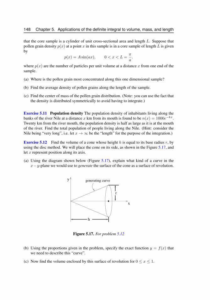
148 Chapter 5. Applications of the definite integral to volume, mass, and length
that the core sample is a cylinder of unit cross-sectional area and length L. Suppose thatpollen grain density p(x) at a point x in this sample is in a core sample of length L is givenby
p(x) = A sin(ax), 0 < x < L =π
a.
where p(x) are the number of particles per unit volume at a distance x from one end of thesample.
(a) Where is the pollen grain most concentrated along this one dimensional sample?
(b) Find the average density of pollen grains along the length of the sample.
(c) Find the center of mass of the pollen grain distribution. (Note: you can use the fact thatthe density is distributed symmetrically to avoid having to integrate.)
Exercise 5.11 Population density The population density of inhabitants living along thebanks of the river Nile at a distance x km from its mouth is found to be n(x) = 1000e−kx.Twenty km from the river mouth, the population density is half as large as it is at the mouthof the river. Find the total population of people living along the Nile. (Hint: consider theNile being “very long”, i.e. let x→∞ be the “length” for the purpose of the integration.)
Exercise 5.12 Find the volume of a cone whose height h is equal to its base radius r, byusing the disc method. We will place the cone on its side, as shown in the Figure 5.17, andlet x represent position along its axis.
(a) Using the diagram shown below (Figure 5.17), explain what kind of a curve in thex−y-plane we would use to generate the surface of the cone as a surface of revolution.
y
x
h
r
generating curve
Figure 5.17. For problem 5.12
(b) Using the proportions given in the problem, specify the exact function y = f(x) thatwe need to describe this “curve”.
(c) Now find the volume enclosed by this surface of revolution for 0 ≤ x ≤ 1.
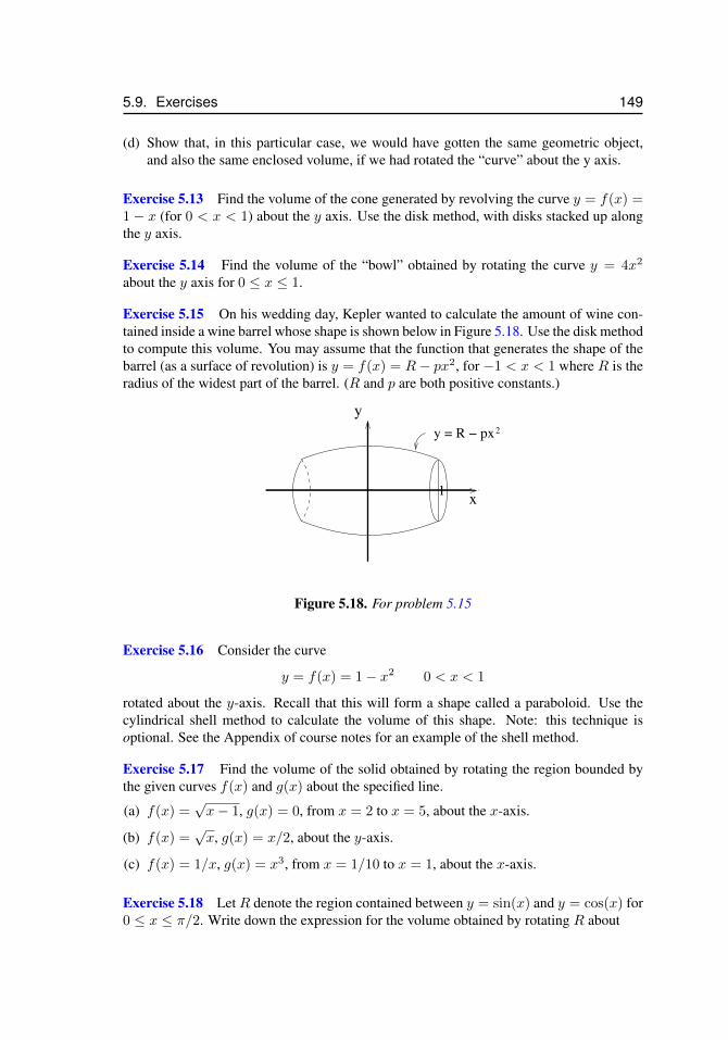
5.9. Exercises 149
(d) Show that, in this particular case, we would have gotten the same geometric object,and also the same enclosed volume, if we had rotated the “curve” about the y axis.
Exercise 5.13 Find the volume of the cone generated by revolving the curve y = f(x) =1 − x (for 0 < x < 1) about the y axis. Use the disk method, with disks stacked up alongthe y axis.
Exercise 5.14 Find the volume of the “bowl” obtained by rotating the curve y = 4x2
about the y axis for 0 ≤ x ≤ 1.
Exercise 5.15 On his wedding day, Kepler wanted to calculate the amount of wine con-tained inside a wine barrel whose shape is shown below in Figure 5.18. Use the disk methodto compute this volume. You may assume that the function that generates the shape of thebarrel (as a surface of revolution) is y = f(x) = R− px2, for −1 < x < 1 where R is theradius of the widest part of the barrel. (R and p are both positive constants.)
x
y
y = R − px2
1
Figure 5.18. For problem 5.15
Exercise 5.16 Consider the curve
y = f(x) = 1− x2 0 < x < 1
rotated about the y-axis. Recall that this will form a shape called a paraboloid. Use thecylindrical shell method to calculate the volume of this shape. Note: this technique isoptional. See the Appendix of course notes for an example of the shell method.
Exercise 5.17 Find the volume of the solid obtained by rotating the region bounded bythe given curves f(x) and g(x) about the specified line.
(a) f(x) =√x− 1, g(x) = 0, from x = 2 to x = 5, about the x-axis.
(b) f(x) =√x, g(x) = x/2, about the y-axis.
(c) f(x) = 1/x, g(x) = x3, from x = 1/10 to x = 1, about the x-axis.
Exercise 5.18 Let R denote the region contained between y = sin(x) and y = cos(x) for0 ≤ x ≤ π/2. Write down the expression for the volume obtained by rotating R about
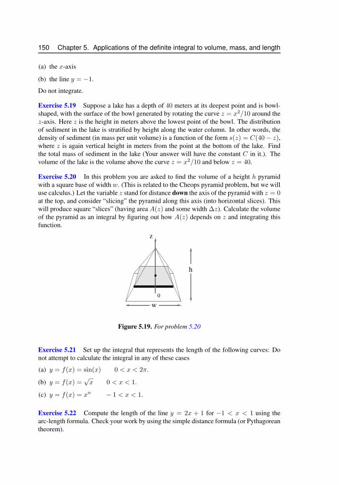
150 Chapter 5. Applications of the definite integral to volume, mass, and length
(a) the x-axis
(b) the line y = −1.
Do not integrate.
Exercise 5.19 Suppose a lake has a depth of 40 meters at its deepest point and is bowl-shaped, with the surface of the bowl generated by rotating the curve z = x2/10 around thez-axis. Here z is the height in meters above the lowest point of the bowl. The distributionof sediment in the lake is stratified by height along the water column. In other words, thedensity of sediment (in mass per unit volume) is a function of the form s(z) = C(40− z),where z is again vertical height in meters from the point at the bottom of the lake. Findthe total mass of sediment in the lake (Your answer will have the constant C in it.). Thevolume of the lake is the volume above the curve z = x2/10 and below z = 40.
Exercise 5.20 In this problem you are asked to find the volume of a height h pyramidwith a square base of width w. (This is related to the Cheops pyramid problem, but we willuse calculus.) Let the variable z stand for distance down the axis of the pyramid with z = 0at the top, and consider “slicing” the pyramid along this axis (into horizontal slices). Thiswill produce square “slices” (having area A(z) and some width ∆z). Calculate the volumeof the pyramid as an integral by figuring out how A(z) depends on z and integrating thisfunction.
z
w
h
0
Figure 5.19. For problem 5.20
Exercise 5.21 Set up the integral that represents the length of the following curves: Donot attempt to calculate the integral in any of these cases
(a) y = f(x) = sin(x) 0 < x < 2π.
(b) y = f(x) =√x 0 < x < 1.
(c) y = f(x) = xn − 1 < x < 1.
Exercise 5.22 Compute the length of the line y = 2x + 1 for −1 < x < 1 using thearc-length formula. Check your work by using the simple distance formula (or Pythagoreantheorem).
5.9. Exercises 151
Exercise 5.23 Spreadsheet assignment You are told that the derivative of a certain func-tion is
f ′(x) = 1− 2 sin2(x/3)
and that f(0) = 0. Use the spreadsheet to create one plot that contains all of the followinggraphs:
(a) The graph of the function y = f(x) (whose derivative is given to you). This should beplotted over the interval from 0 to 9.
(b) The graph of the “element of arc-length” dl =√
1 + (f ′(x))2dx showing how thisvaries across the same interval.
(c) The graph of the cumulative length of the curve L(x). Briefly indicate what you didto find the function in part (a). (You might consider how the spreadsheet would helpyou calculate the values of the desired function, y = f(x), rather than trying to find anexpression for it.)
Exercise 5.24 Work of spring A spring has a natural length of 16 cm. When it is stretchedx cm beyond that, Hooke’s Law states that the spring pulls back with a restoring forceF = kx dyne, where the constant k is called the spring constant, and represents the stiffnessof the spring. For the given spring, 8 dyne of force are required to hold it stretched by2 cm. How much work (dyne-cm) is done in stretching this spring from its natural lengthto a length 24 cm? (Note: use integration to set up this problem.)
Exercise 5.25 Work of pump Calculate the work done in pumping water out of a paraboliccontainer up to the height h = 10 units. Assume that the container is a surface of revolutiongenerated by rotating the curve y = x2 about the y axis, that the height of the water in thecontainer is 10 units, that the density of water is 1 g/cm3 and that the force due to gravityis F = mg where m is mass and g = 9.8 m/s2.

152 Chapter 5. Applications of the definite integral to volume, mass, and length
Chapter 6
Techniques ofIntegration
In this chapter, we expand our repertoire for antiderivatives beyond the “elementary” func-tions discussed so far. A review of the table of elementary antiderivatives (found in Chap-ter 3) will be useful. Here we will discuss a number of methods for finding antiderivatives.We refer to these collected “tricks” as methods of integration. As will be shown, in somecases, these methods are systematic (i.e. with clear steps), whereas in other cases, guess-work and trial and error is an important part of the process.
A primary method of integration to be described is substitution. A close relationshipexists between the chain rule of differential calculus and the substitution method. A secondvery important method is integration by parts. Aside from its usefulness in integrationper se, this method has numerous applications in physics, mathematics, and other sciences.Many other techniques of integration used to form a core of methods taught in such coursesin integral calculus. Many of these are quite technical. Nowadays, with sophisticatedmathematical software packages (including Maple and Mathematica), integration can becarried our automatically via computation called “symbolic manipulation”, reducing ourneed to dwell on these technical methods.
6.1 Differential notationWe begin by familiarizing the reader with notation that appears frequently in substitutionintegrals, i.e. differential notation. Consider a straight line
y = mx+ b.
Recall that the slope of the line, m, is
m =change in ychange in x
=∆y
∆x.
This relationship can also be written in the form
∆y = m∆x.
153
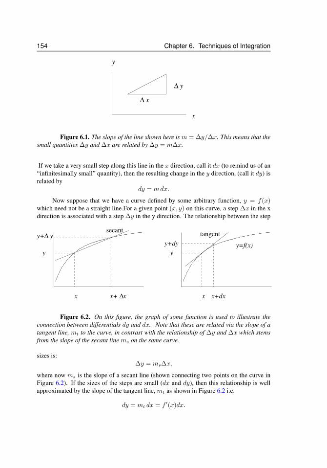
154 Chapter 6. Techniques of Integration
y
x∆
∆
x
y
Figure 6.1. The slope of the line shown here is m = ∆y/∆x. This means that thesmall quantities ∆y and ∆x are related by ∆y = m∆x.
If we take a very small step along this line in the x direction, call it dx (to remind us of an“infinitesimally small” quantity), then the resulting change in the y direction, (call it dy) isrelated by
dy = mdx.
Now suppose that we have a curve defined by some arbitrary function, y = f(x)which need not be a straight line.For a given point (x, y) on this curve, a step ∆x in the xdirection is associated with a step ∆y in the y direction. The relationship between the step
y=f(x)
x
y
x+ ∆x
y+∆ y
x
y
x+dx
y+dy
secanttangent
Figure 6.2. On this figure, the graph of some function is used to illustrate theconnection between differentials dy and dx. Note that these are related via the slope of atangent line, mt to the curve, in contrast with the relationship of ∆y and ∆x which stemsfrom the slope of the secant line ms on the same curve.
sizes is:∆y = ms∆x,
where now ms is the slope of a secant line (shown connecting two points on the curve inFigure 6.2). If the sizes of the steps are small (dx and dy), then this relationship is wellapproximated by the slope of the tangent line, mt as shown in Figure 6.2 i.e.
dy = mt dx = f ′(x)dx.
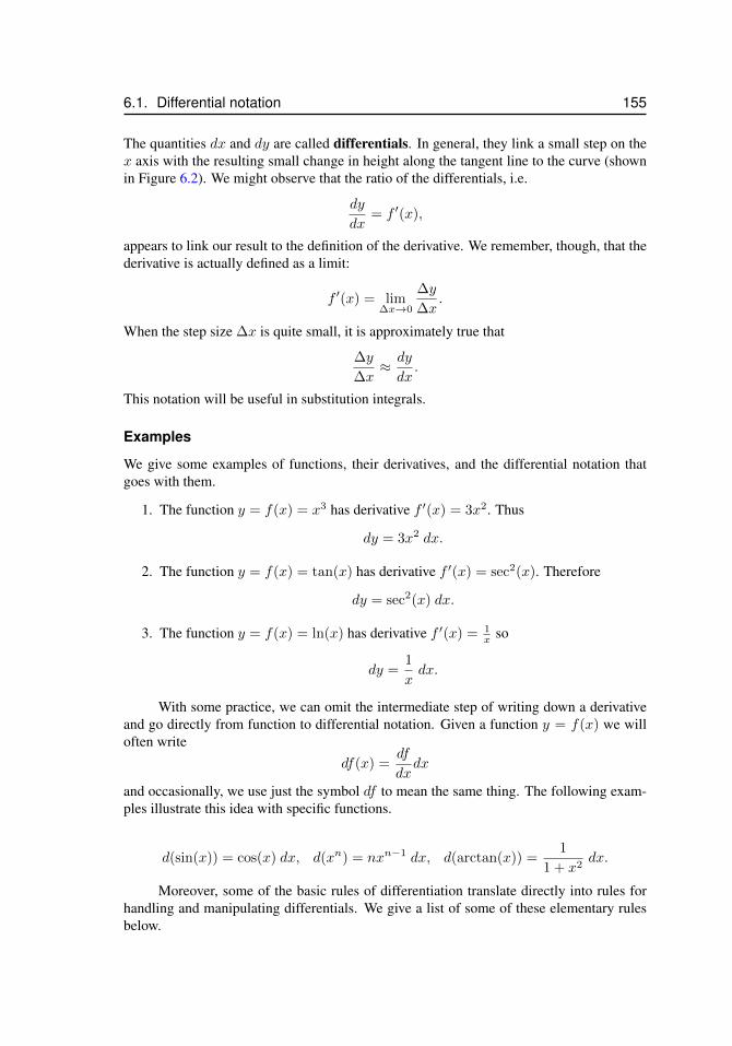
6.1. Differential notation 155
The quantities dx and dy are called differentials. In general, they link a small step on thex axis with the resulting small change in height along the tangent line to the curve (shownin Figure 6.2). We might observe that the ratio of the differentials, i.e.
dy
dx= f ′(x),
appears to link our result to the definition of the derivative. We remember, though, that thederivative is actually defined as a limit:
f ′(x) = lim∆x→0
∆y
∆x.
When the step size ∆x is quite small, it is approximately true that
∆y
∆x≈ dy
dx.
This notation will be useful in substitution integrals.
Examples
We give some examples of functions, their derivatives, and the differential notation thatgoes with them.
1. The function y = f(x) = x3 has derivative f ′(x) = 3x2. Thus
dy = 3x2 dx.
2. The function y = f(x) = tan(x) has derivative f ′(x) = sec2(x). Therefore
dy = sec2(x) dx.
3. The function y = f(x) = ln(x) has derivative f ′(x) = 1x so
dy =1
xdx.
With some practice, we can omit the intermediate step of writing down a derivativeand go directly from function to differential notation. Given a function y = f(x) we willoften write
df(x) =df
dxdx
and occasionally, we use just the symbol df to mean the same thing. The following exam-ples illustrate this idea with specific functions.
d(sin(x)) = cos(x) dx, d(xn) = nxn−1 dx, d(arctan(x)) =1
1 + x2dx.
Moreover, some of the basic rules of differentiation translate directly into rules forhandling and manipulating differentials. We give a list of some of these elementary rulesbelow.
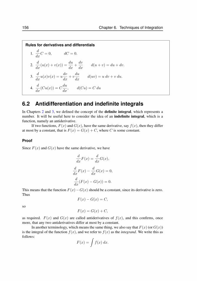
156 Chapter 6. Techniques of Integration
Rules for derivatives and differentials
1.d
dxC = 0, dC = 0.
2.d
dx(u(x) + v(x)) =
du
dx+dv
dxd(u+ v) = du+ dv.
3.d
dxu(x)v(x) = u
dv
dx+ v
du
dxd(uv) = u dv + v du.
4.d
dx(Cu(x)) = C
du
dx, d(Cu) = C du
6.2 Antidifferentiation and indefinite integralsIn Chapters 2 and 3, we defined the concept of the definite integral, which represents anumber. It will be useful here to consider the idea of an indefinite integral, which is afunction, namely an antiderivative.
If two functions, F (x) and G(x), have the same derivative, say f(x), then they differat most by a constant, that is F (x) = G(x) + C, where C is some constant.
Proof
Since F (x) and G(x) have the same derivative, we have
d
dxF (x) =
d
dxG(x),
d
dxF (x)− d
dxG(x) = 0,
d
dx(F (x)−G(x)) = 0.
This means that the function F (x)−G(x) should be a constant, since its derivative is zero.Thus
F (x)−G(x) = C,
soF (x) = G(x) + C,
as required. F (x) and G(x) are called antiderivatives of f(x), and this confirms, oncemore, that any two antiderivatives differ at most by a constant.
In another terminology, which means the same thing, we also say that F (x) (orG(x))is the integral of the function f(x), and we refer to f(x) as the integrand. We write this asfollows:
F (x) =
∫f(x) dx.
6.2. Antidifferentiation and indefinite integrals 157
This notation is sometimes called “an indefinite integral” because it does not denote aspecific numerical value, nor is an interval specified for the integration range. An indefiniteintegral is a function with an arbitrary constant. (Contrast this with the definite integralstudied in our last chapters: in the case of the definite integral, we specified an interval, andinterpreted the result, a number, in terms of areas associated with curves.) We also write∫
f(x) dx = F (x) + C,
if we want to indicate the form of all possible functions that are antiderivatives of f(x). Cis referred to as a constant of integration.
6.2.1 Integrals of derivativesSuppose we are given an integral of the form∫
df
dxdx,
or alternately, the same thing written using differential notation,∫df.
How do we handle this? We reason as follows. The df/dx (a quantity that is, itself, afunction) is the derivative of the function f(x). That means that f(x) is the antiderivativeof df/dx. Then, according to the Fundamental Theorem of Calculus,∫
df
dxdx = f(x) + C.
We can write this same result using the differential of f , as follows:∫df = f(x) + C.
The following examples illustrate the idea with several elementary functions.
Examples
1.∫d(cosx) = cosx+ C.
2.∫dv = v + C.
3.∫d(x3) = x3 + C.
158 Chapter 6. Techniques of Integration
6.3 Simple substitutionIn this section, we observe that the forms of some integrals can be simplified by making ajudicious substitution, and using our familiarity with derivatives (and the chain rule). Theidea rests on the fact that in some cases, we can spot a “helper function”
u = f(x),
such that the quantitydu = f ′(x)dx
appears in the integrand. In that case, the substitution will lead to eliminating x entirely infavour of the new quantity u, and simplification may occur.
6.3.1 Example: Simple substitutionSuppose we are given the function
f(x) = (x+ 1)10.
Then its antiderivative (indefinite integral) is
F (x) =
∫f(x) dx =
∫(x+ 1)10 dx.
We could find an antiderivative by expanding the integrand (x + 1)10 into a degree 10polynomial and using methods already known to us; but this would be laborious. Let usobserve, however, that if we define
u = (x+ 1),
then
du =d(x+ 1)
dxdx =
(dx
dx+d(1)
dx
)dx = (1 + 0)dx = dx.
Now replacing (x+ 1) by u and dx by the equivalent du we get:
F (x) =
∫u10du.
An antiderivative to this can be easily found, namely,
F (x) =u11
11=
(x+ 1)11
11+ C.
In the last step, we converted the result back to the original variable, and included thearbitrary integration constant. A very important point to remember is that we can alwayscheck our results by differentiation:
Check
Differentiate F (x) to obtain
dF
dx=
1
11(11(x+ 1)10) = (x+ 1)10.
6.3. Simple substitution 159
6.3.2 How to handle endpointsWe consider how substitution type integrals can be calculated when we have endpoints, i.e.in evaluating definite integrals. Consider the example:
I =
∫ 2
1
1
x+ 1dx .
This integration can be done by making the substitution u = x+ 1 for which du = dx. Wecan handle the endpoints in one of two ways:
Method 1: Change the endpoints
We can change the integral over entirely to a definite integral in the variable u as follows:Since u = x + 1, the endpoint x = 1 corresponds to u = 2, and the endpoint x = 2corresponds to u = 3, so changing the endpoints to reflect the change of variables leads to
I =
∫ 3
2
1
udu = ln |u|
∣∣∣∣32
= ln 3− ln 2 = ln3
2.
In the last steps we have plugged in the new endpoints (appropriate to u).
Method 2: Change back to x before evaluating at endpoints
Alternately, we could rewrite the antiderivative in terms of x.∫1
udu = ln |u|+ C = ln |x+ 1|+ C
and then evaluate this function at the original endpoints.∫ 2
1
1
x+ 1dx = ln |x+ 1|
∣∣∣∣21
= ln3
2
Here we plugged in the original endpoints (as appropriate to the variable x). Notice thatwhen evaluating the antiderivative at the endpoints the integration constant can be ignoredas it cancels (c.f. second part of Fundamental Theorem of Calculus, Section 3.4.3).
6.3.3 Examples: Substitution type integralsFind a simple substitution and determine the antiderivatives (indefinite or definite integrals)of the following functions:
1. I =
∫2
x+ 2dx.
2. I =
∫ 1
0
x2ex3
dx
160 Chapter 6. Techniques of Integration
3. I =
∫1
(x+ 1)2 + 1dx.
4. I =
∫(x+ 3)
√x2 + 6x+ 10 dx.
5. I =
∫ π
0
cos3(x) sin(x) dx.
6. I =
∫1
ax+ bdx
7. I =
∫1
b+ ax2dx.
Solutions
1. I =
∫2
x+ 2dx. Let u = x+ 2. Then du = dx and we get
I =
∫2
udu = 2
∫1
udu = 2 ln |u| = 2 ln |x+ 2|+ C.
2. I =
∫ 1
0
x2ex3
dx. Let u = x3. Then du = 3x2 dx. Here we use method 2 for
handling endpoints. ∫eudu
3=
1
3eu =
1
3ex
3
+ C.
Then
I =
∫ 1
0
x2ex3
dx =1
3ex
3
∣∣∣∣10
=1
3(e− 1).
(We converted the antiderivative to the original variable, x, before plugging in theoriginal endpoints.)
3. I =
∫1
(x+ 1)2 + 1dx. Let u = x+ 1, then du = dx so we have
I =
∫1
u2 + 1du = arctan(u) = arctan(x+ 1) + C.
4. I =
∫(x+3)
√x2 + 6x+ 10 dx. Let u = x2 +6x+10. Then du = (2x+6) dx =
2(x+ 3) dx. With this substitution we get
I =
∫ √udu
2=
1
2
∫u1/2 du =
1
2
u3/2
3/2=
1
3u3/2 =
1
3(x2 + 6x+ 10)3/2 + C.
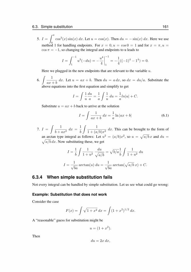
6.3. Simple substitution 161
5. I =
∫ π
0
cos3(x) sin(x) dx. Let u = cos(x). Then du = − sin(x) dx. Here we use
method 1 for handling endpoints. For x = 0, u = cos 0 = 1 and for x = π, u =cosπ = −1, so changing the integral and endpoints to u leads to
I =
∫ −1
1
u3(−du) = −u4
4
∣∣∣∣−1
1
= −1
4((−1)4 − 14) = 0.
Here we plugged in the new endpoints that are relevant to the variable u.
6.∫
1
ax+ bdx. Let u = ax + b. Then du = a dx, so dx = du/a. Substitute the
above equations into the first equation and simplify to get
I =
∫1
u
du
a=
1
a
∫1
udu =
1
aln|u|+ C.
Substitute u = ax+ b back to arrive at the solution
I =
∫1
ax+ bdx =
1
aln |ax+ b| (6.1)
7. I =
∫1
b+ ax2dx =
1
b
∫1
1 + (a/b)x2dx. This can be brought to the form of
an arctan type integral as follows: Let u2 = (a/b)x2, so u =√a/b x and du =√
a/b dx. Now substituting these, we get
I =1
b
∫1
1 + u2
du√a/b
=√b/a
1
b
∫1
1 + u2du
I =1√ba
arctan(u) du =1√ba
arctan(√a/b x) + C.
6.3.4 When simple substitution failsNot every integral can be handled by simple substitution. Let us see what could go wrong:
Example: Substitution that does not work
Consider the case
F (x) =
∫ √1 + x2 dx =
∫(1 + x2)1/2 dx.
A “reasonable” guess for substitution might be
u = (1 + x2).
Thendu = 2x dx,
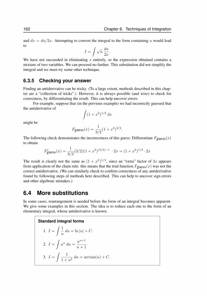
162 Chapter 6. Techniques of Integration
and dx = du/2x. Attempting to convert the integral to the form containing u would leadto
I =
∫ √udu
2x.
We have not succeeded in eliminating x entirely, so the expression obtained contains amixture of two variables. We can proceed no further. This substitution did not simplify theintegral and we must try some other technique.
6.3.5 Checking your answerFinding an antiderivative can be tricky. (To a large extent, methods described in this chap-ter are a “collection of tricks”.) However, it is always possible (and wise) to check forcorrectness, by differentiating the result. This can help uncover errors.
For example, suppose that (in the previous example) we had incorrectly guessed thatthe antiderivative of ∫
(1 + x2)1/2 dx
might be
Fguess(x) =1
3/2(1 + x2)3/2.
The following check demonstrates the incorrectness of this guess: Differentiate Fguess(x)to obtain
F ′guess(x) =1
3/2(3/2)(1 + x2)(3/2)−1 · 2x = (1 + x2)1/2 · 2x
The result is clearly not the same as (1 + x2)1/2, since an “extra” factor of 2x appearsfrom application of the chain rule: this means that the trial function Fguess(x) was not thecorrect antiderivative. (We can similarly check to confirm correctness of any antiderivativefound by following steps of methods here described. This can help to uncover sign errorsand other algebraic mistakes.)
6.4 More substitutionsIn some cases, rearrangement is needed before the form of an integral becomes apparent.We give some examples in this section. The idea is to reduce each one to the form of anelementary integral, whose antiderivative is known.
Standard integral forms
1. I =
∫1
udu = ln |u|+ C.
2. I =
∫un du =
un+1
n+ 1.
3. I =
∫1
1 + u2du = arctan(u) + C.
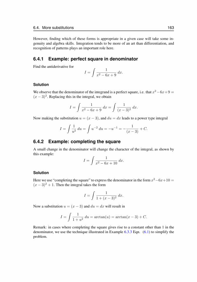
6.4. More substitutions 163
However, finding which of these forms is appropriate in a given case will take some in-genuity and algebra skills. Integration tends to be more of an art than differentiation, andrecognition of patterns plays an important role here.
6.4.1 Example: perfect square in denominatorFind the antiderivative for
I =
∫1
x2 − 6x+ 9dx.
Solution
We observe that the denominator of the integrand is a perfect square, i.e. that x2−6x+9 =(x− 3)2. Replacing this in the integral, we obtain
I =
∫1
x2 − 6x+ 9dx =
∫1
(x− 3)2dx.
Now making the substitution u = (x− 3), and du = dx leads to a power type integral
I =
∫1
u2du =
∫u−2 du = −u−1 = − 1
(x− 3)+ C.
6.4.2 Example: completing the squareA small change in the denominator will change the character of the integral, as shown bythis example:
I =
∫1
x2 − 6x+ 10dx.
Solution
Here we use “completing the square” to express the denominator in the form x2−6x+10 =(x− 3)2 + 1. Then the integral takes the form
I =
∫1
1 + (x− 3)2dx.
Now a substitution u = (x− 3) and du = dx will result in
I =
∫1
1 + u2du = arctan(u) = arctan(x− 3) + C.
Remark: in cases where completing the square gives rise to a constant other than 1 in thedenominator, we use the technique illustrated in Example 6.3.3 Eqn. (6.1) to simplify theproblem.
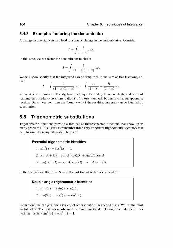
164 Chapter 6. Techniques of Integration
6.4.3 Example: factoring the denominatorA change in one sign can also lead to a drastic change in the antiderivative. Consider
I =
∫1
1− x2dx.
In this case, we can factor the denominator to obtain
I =
∫1
(1− x)(1 + x)dx.
We will show shortly that the integrand can be simplified to the sum of two fractions, i.e.that
I =
∫1
(1− x)(1 + x)dx =
∫A
(1− x)+
B
(1 + x)dx,
whereA,B are constants. The algebraic technique for finding these constants, and hence offorming the simpler expressions, called Partial fractions, will be discussed in an upcomingsection. Once these constants are found, each of the resulting integrals can be handled bysubstitution.
6.5 Trigonometric substitutionsTrigonometric functions provide a rich set of interconnected functions that show up inmany problems. It is useful to remember three very important trigonometric identities thathelp to simplify many integrals. These are:
Essential trigonometric identities
1. sin2(x) + cos2(x) = 1
2. sin(A+B) = sin(A) cos(B) + sin(B) cos(A)
3. cos(A+B) = cos(A) cos(B)− sin(A) sin(B).
In the special case that A = B = x, the last two identities above lead to:
Double angle trigonometric identities
1. sin(2x) = 2 sin(x) cos(x).
2. cos(2x) = cos2(x)− sin2(x).
From these, we can generate a variety of other identities as special cases. We list the mostuseful below. The first two are obtained by combining the double-angle formula for cosineswith the identity sin2(x) + cos2(x) = 1.
6.5. Trigonometric substitutions 165
Useful trigonometric identities
1. cos2(x) =1 + cos(2x)
2.
2. sin2(x) =1− cos(2x)
2.
3. tan2(x) + 1 = sec2(x).
6.5.1 Example: simple trigonometric substitutionFind the antiderivative of
I =
∫sin(x) cos2(x) dx.
Solution
This integral can be computed by a simple substitution, similar to Example 5 of Section 6.3.We let u = cos(x) and du = − sin(x)dx to get the integral into the form
I = −∫u2 du =
−u3
3=− cos3(x)
3+ C.
We need none of the trigonometric identities in this case. Simple substitution is always theeasiest method to use. It should be the first method attempted in each case.
6.5.2 Example: using trigonometric identities (1)Find the antiderivative of
I =
∫cos2(x) dx.
Solution
This is an example in which the “Useful trigonometric identity” 1 leads to a simpler inte-gral. We write
I =
∫cos2(x) dx =
∫1 + cos(2x)
2dx =
1
2
∫(1 + cos(2x)) dx.
Then clearly,
I =1
2
(x+
sin(2x)
2
)+ C.
6.5.3 Example: using trigonometric identities (2)Find the antiderivative of
I =
∫sin3(x) dx.
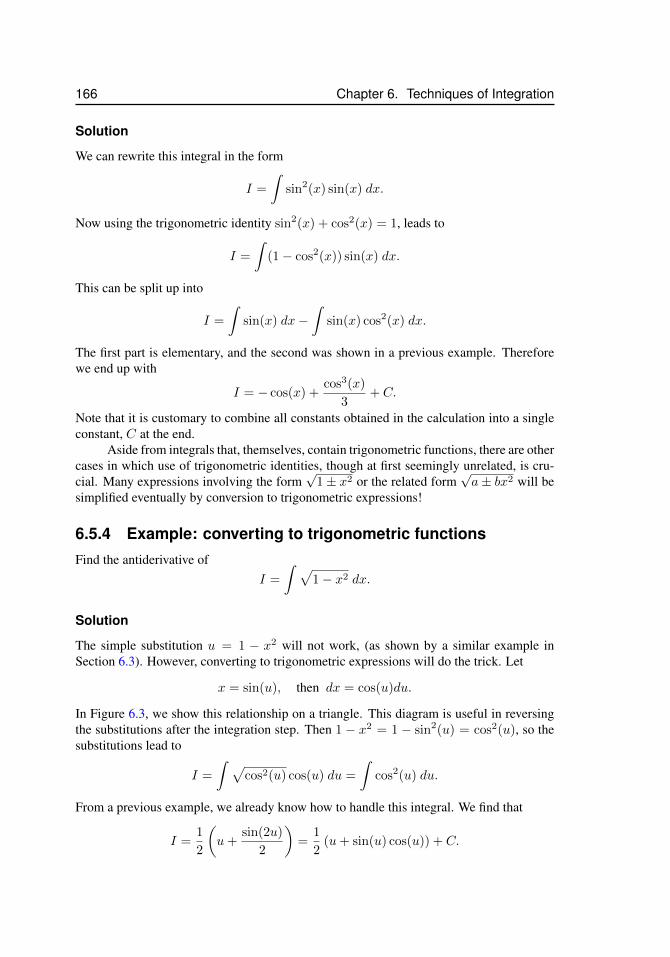
166 Chapter 6. Techniques of Integration
Solution
We can rewrite this integral in the form
I =
∫sin2(x) sin(x) dx.
Now using the trigonometric identity sin2(x) + cos2(x) = 1, leads to
I =
∫(1− cos2(x)) sin(x) dx.
This can be split up into
I =
∫sin(x) dx−
∫sin(x) cos2(x) dx.
The first part is elementary, and the second was shown in a previous example. Thereforewe end up with
I = − cos(x) +cos3(x)
3+ C.
Note that it is customary to combine all constants obtained in the calculation into a singleconstant, C at the end.
Aside from integrals that, themselves, contain trigonometric functions, there are othercases in which use of trigonometric identities, though at first seemingly unrelated, is cru-cial. Many expressions involving the form
√1± x2 or the related form
√a± bx2 will be
simplified eventually by conversion to trigonometric expressions!
6.5.4 Example: converting to trigonometric functionsFind the antiderivative of
I =
∫ √1− x2 dx.
Solution
The simple substitution u = 1 − x2 will not work, (as shown by a similar example inSection 6.3). However, converting to trigonometric expressions will do the trick. Let
x = sin(u), then dx = cos(u)du.
In Figure 6.3, we show this relationship on a triangle. This diagram is useful in reversingthe substitutions after the integration step. Then 1 − x2 = 1 − sin2(u) = cos2(u), so thesubstitutions lead to
I =
∫ √cos2(u) cos(u) du =
∫cos2(u) du.
From a previous example, we already know how to handle this integral. We find that
I =1
2
(u+
sin(2u)
2
)=
1
2(u+ sin(u) cos(u)) + C.
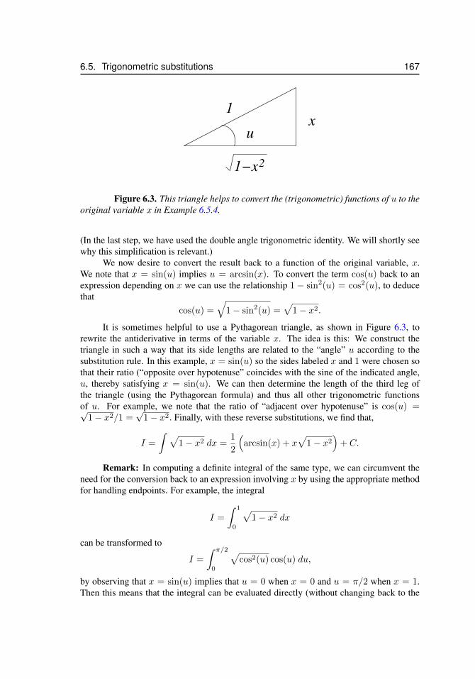
6.5. Trigonometric substitutions 167
x1
1−x2
u
Figure 6.3. This triangle helps to convert the (trigonometric) functions of u to theoriginal variable x in Example 6.5.4.
(In the last step, we have used the double angle trigonometric identity. We will shortly seewhy this simplification is relevant.)
We now desire to convert the result back to a function of the original variable, x.We note that x = sin(u) implies u = arcsin(x). To convert the term cos(u) back to anexpression depending on x we can use the relationship 1 − sin2(u) = cos2(u), to deducethat
cos(u) =
√1− sin2(u) =
√1− x2.
It is sometimes helpful to use a Pythagorean triangle, as shown in Figure 6.3, torewrite the antiderivative in terms of the variable x. The idea is this: We construct thetriangle in such a way that its side lengths are related to the “angle” u according to thesubstitution rule. In this example, x = sin(u) so the sides labeled x and 1 were chosen sothat their ratio (“opposite over hypotenuse” coincides with the sine of the indicated angle,u, thereby satisfying x = sin(u). We can then determine the length of the third leg ofthe triangle (using the Pythagorean formula) and thus all other trigonometric functionsof u. For example, we note that the ratio of “adjacent over hypotenuse” is cos(u) =√
1− x2/1 =√
1− x2. Finally, with these reverse substitutions, we find that,
I =
∫ √1− x2 dx =
1
2
(arcsin(x) + x
√1− x2
)+ C.
Remark: In computing a definite integral of the same type, we can circumvent theneed for the conversion back to an expression involving x by using the appropriate methodfor handling endpoints. For example, the integral
I =
∫ 1
0
√1− x2 dx
can be transformed to
I =
∫ π/2
0
√cos2(u) cos(u) du,
by observing that x = sin(u) implies that u = 0 when x = 0 and u = π/2 when x = 1.Then this means that the integral can be evaluated directly (without changing back to the
168 Chapter 6. Techniques of Integration
variable x) as follows:
I =
∫ π/2
0
√cos2(u) cos(u) du =
1
2
(u+
sin(2u)
2
) ∣∣∣∣π/20
=1
2
(π
2+
sin(π)
2
)=π
4
where we have used the fact that sin(π) = 0.Some subtle points about the domains of definition of inverse trigonometric functions
will not be discussed here in detail. (See material on these functions in a first term calculuscourse.) Suffice it to say that some integrals of this type will be undefined if this endpointconversion cannot be carried out (e.g. if the interval of integration had been 0 ≤ x ≤ 2,we would encounter an impossible relation 2 = sin(u). Since no value of u satisfies thisrelation, such a definite integral has no meaning, i.e. “does not exist”.)
6.5.5 Example: The centroid of a two dimensional shapeWe extend the concept of centroid (center of mass) for a region that has uniform densityin 2D, but where we consider the distribution of mass along the x (or y) axis. Considerthe semicircle shape of uniform thickness, shown in Figure 6.4, and suppose it is balancedalong its horizontal edge. Find the x coordinate c at which the shape balances.
x
y
y= 9 − x 2
Figure 6.4. A semicircular shape.
Solution
The semicircle is one quarter of a circle of radius 3. Its edge is described by the equation
y = f(x) =√
9− x2.
We will assume that the density per unit area is uniform. However, the mass per unitlength along the x axis is not uniform, due to the shape of the object. We apply the idea ofintegration: If we cut the shape at increments of ∆x along the x axis, we get a collectionof pieces whose mass is each proportional to f(x)∆x. Summing up such contributions andletting the widths ∆x→ dx get small, we arrive at the integral for mass. The total mass ofthe shape is thus
M =
∫ 3
0
f(x) dx =
∫ 3
0
√9− x2 dx.
6.5. Trigonometric substitutions 169
Furthermore, if we compute the integral
I =
∫ 3
0
xf(x) dx =
∫ 3
0
x√
9− x2 dx,
we obtain the x coordinate of the center of mass,
x =I
M.
It is evident that the mass is proportional to the area of one quarter of a circle of radius 3:
M =1
4π(3)2 =
9
4π.
(We could also see this by performing a trigonometric substitution integral.) The secondintegral can be done by simple substitution. Consider
I =
∫ 3
0
xf(x) dx =
∫ 3
0
x√
9− x2 dx.
Let u = 9 − x2. Then du = −2x dx. The endpoints are converted as follows: x = 0 ⇒u = 9− 02 = 9 and x = 3⇒ u = 9− 32 = 0 so that we get the integral
I =
∫ 0
9
√u
1
−2du.
We can reverse the endpoints if we switch the sign, and this leads to
I =1
2
∫ 9
0
u1/2 du =
(1
2
)(u3/2
3/2
) ∣∣∣∣90
.
Since 93/2 = (91/2)3 = 33, we get I = (33)/3 = 32 = 9. Thus the x coordinate of thecenter of mass is
x =I
M=
9
(9/4)π=
4
π.
We can similarly find the y coordinate of the center of mass: To do so, we would expressthe boundary of the shape in the form x = f(y) and integrate to find
y =
∫ 3
0
yf(y) dy.
For the semicircle, y2 + x2 = 9, so x = f(y) =√
9− y2. Thus
y =
∫ 3
0
y√
9− y2 dy.
This integral looks identical to the one we wrote down for x. Thus, based on this similarity(or based on the symmetry of the problem) we will find that
y =4
π.
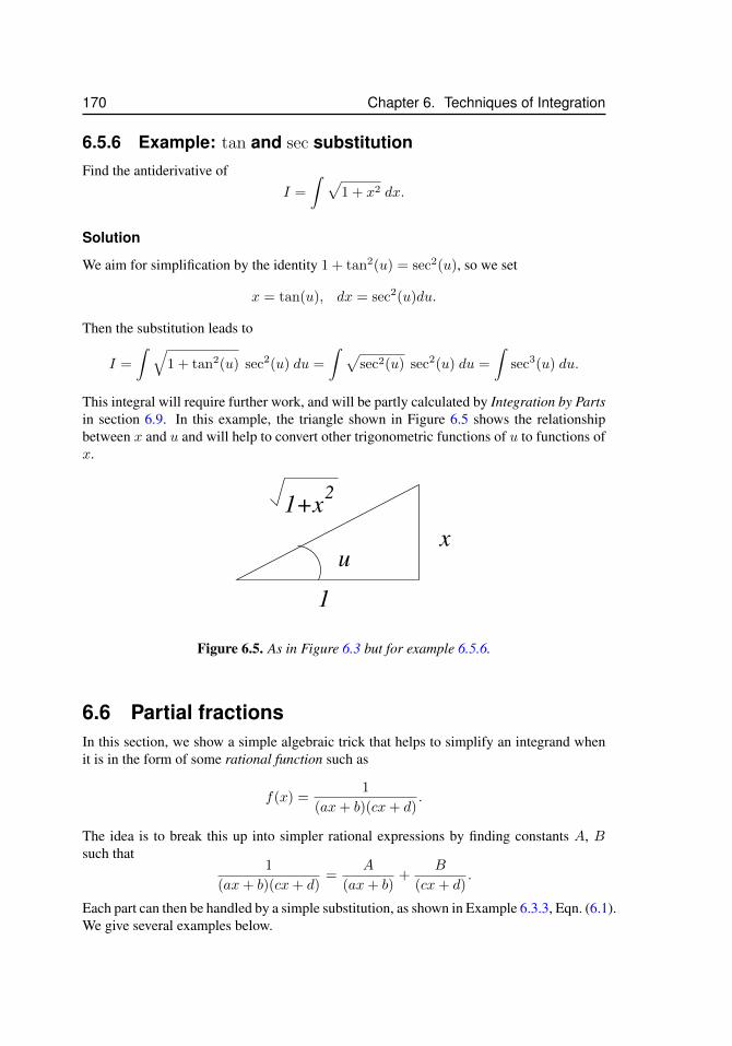
170 Chapter 6. Techniques of Integration
6.5.6 Example: tan and sec substitutionFind the antiderivative of
I =
∫ √1 + x2 dx.
Solution
We aim for simplification by the identity 1 + tan2(u) = sec2(u), so we set
x = tan(u), dx = sec2(u)du.
Then the substitution leads to
I =
∫ √1 + tan2(u) sec2(u) du =
∫ √sec2(u) sec2(u) du =
∫sec3(u) du.
This integral will require further work, and will be partly calculated by Integration by Partsin section 6.9. In this example, the triangle shown in Figure 6.5 shows the relationshipbetween x and u and will help to convert other trigonometric functions of u to functions ofx.
xu
1+x2
1
Figure 6.5. As in Figure 6.3 but for example 6.5.6.
6.6 Partial fractionsIn this section, we show a simple algebraic trick that helps to simplify an integrand whenit is in the form of some rational function such as
f(x) =1
(ax+ b)(cx+ d).
The idea is to break this up into simpler rational expressions by finding constants A, Bsuch that
1
(ax+ b)(cx+ d)=
A
(ax+ b)+
B
(cx+ d).
Each part can then be handled by a simple substitution, as shown in Example 6.3.3, Eqn. (6.1).We give several examples below.
6.6. Partial fractions 171
6.6.1 Example: partial fractions (1)Find the antiderivative of
I =
∫1
x2 − 1.
Factoring the denominator, x2 − 1 = (x − 1)(x + 1), suggests breaking up the integrandinto the form
1
x2 − 1=
A
(x+ 1)+
B
(x− 1).
The two sides are equal provided:
1
x2 − 1=A(x− 1) +B(x+ 1)
x2 − 1.
This means that1 = A(x− 1) +B(x+ 1)
must be true for all x values. We now ask what values of A and B make this equation holdfor any x. Choosing two “easy” values, namely x = 1 and x = −1 leads to isolating oneor the other unknown constants, A,B, with the results:
1 = −2A, 1 = 2B.
Thus B = 1/2, A = −1/2, so the integral can be written in the simpler form
I =1
2
(∫−1
(x+ 1)dx+
∫1
(x− 1)dx
).
(A common factor of (1/2) has been taken out.) Now a simple substitution will work foreach component. (Let u = x+ 1 for the first, and u = x− 1 for the second integral.) Theresult is
I =
∫1
x2 − 1=
1
2(− ln |x+ 1|+ ln |x− 1|) + C.
6.6.2 Example: partial fractions (2)Find the antiderivative of
I =
∫1
x(1− x)dx.
This example is similar to the previous one. We set
1
x(1− x)=A
x+
B
(1− x).
Then1 = A(1− x) +Bx.
This must hold for all x values. In particular, convenient values of x for determining theconstants are x = 0, 1. We find that
A = 1, B = 1.
172 Chapter 6. Techniques of Integration
ThusI =
∫1
x(1− x)dx =
∫1
xdx+
∫1
1− xdx.
Simple substitution now gives
I = ln |x| − ln |1− x|+ C.
6.6.3 Example: partial fractions (3)Find the antiderivative of
I =
∫x
x2 + x− 2.
The rational expression above factors into x2 + x − 2 = (x − 1)(x + 2), leading to theexpression
x
x2 + x− 2=
A
(x− 1)+
B
(x+ 2).
Consequently, it follows that
A(x+ 2) +B(x− 1) = x.
Substituting the values x = 1,−2 into this leads to A = 1/3 and B = 2/3. The usualprocedure then results in
I =
∫x
x2 + x− 2=
1
3ln |x− 1|+ 2
3ln |x+ 2|+ C.
Another example of the technique of partial fractions is provided in section 6.9.2.
6.7 Integration by partsThe method described in this section is important as an additional tool for integration. Italso has independent theoretical stature in many applications in mathematics and physics.The essential idea is that in some cases, we can exchange the task of integrating a functionwith the job of differentiating it.
The idea rests on the product rule for derivatives. Suppose that u(x) and v(x) aretwo differentiable functions. Then we know that the derivative of their product is
d(uv)
dx= v
du
dx+ u
dv
dx,
or, in the differential notation:
d(uv) = v du+ u dv,
Integrating both sides, we obtain∫d(uv) =
∫v du+
∫u dv
6.7. Integration by parts 173
i.e.uv =
∫v du+
∫u dv.
We write this result in the more suggestive form∫u dv = uv −
∫v du.
The idea here is that if we have difficulty evaluating an integral such as∫u dv, we may be
able to “exchange it” for a simpler integral in the form∫v du. This is best illustrated by
the examples below.
Example: Integration by parts (1)
Compute
I =
∫ 2
1
ln(x) dx.
Solution
Let u = ln(x) and dv = dx. Then du = (1/x) dx and v = x.∫ln(x) dx = x ln(x)−
∫x(1/x) dx = x ln(x)−
∫dx = x ln(x)− x.
We now evaluate this result at the endpoints to obtain
I =
∫ 2
1
ln(x) dx = (x ln(x)− x)
∣∣∣∣21
= (2 ln(2)− 2)− (1 ln(1)− 1) = 2 ln(2)− 1.
(Where we used the fact that ln(1) = 0.)
Example: Integration by parts (2)
Compute
I =
∫ 1
0
xex dx.
Solution
At first, it may be hard to decide how to assign roles for u and dv. Suppose we try u = ex
and dv = xdx. Then du = ex dx and v = x2/2. This means that we would get the integralin the form
I =x2
2ex −
∫x2
2ex dx.
This is certainly not a simplification, because the integral we obtain has a higher power ofx, and is consequently harder, not easier to integrate. This suggests that our first attemptwas not a helpful one. (Note that integration often requires trial and error.)
174 Chapter 6. Techniques of Integration
Let u = x and dv = ex dx. This is a wiser choice because when we differentiate u,we reduce the power of x (from 1 to 0), and get a simpler expression. Indeed, du = dx,v = ex so that ∫
xex dx = xex −∫ex dx = xex − ex + C.
To find a definite integral of this kind on some interval (say 0 ≤ x ≤ 1), we compute
I =
∫ 1
0
xex dx = (xex − ex)
∣∣∣∣10
= (1e1 − e1)− (0e0 − e0) = 0 + e0 = e0 = 1.
Note that all parts of the expression are evaluated at the two endpoints.
Example: Integration by parts (2b)
Compute
In =
∫xnex dx.
Solution
We can calculate this integral by repeated application of the idea in the previous example.Letting u = xn and dv = ex dx leads to du = nxn−1 and v = ex. Then
In = xnex −∫nxn−1ex dx = xnex − n
∫xn−1ex dx.
Each application of integration by parts, reduces the power of the term xn inside an integralby one. The calculation is repeated until the very last integral has been simplified, withno remaining powers of x. This illustrates that in some problems, integration by parts isneeded more than once.
Example: Integration by parts (3)
Compute
I =
∫arctan(x) dx.
Solution
Let u = arctan(x) and dv = dx. Then du = (1/(1 + x2)) dx and v = x so that
I = x arctan(x)−∫
1
1 + x2x dx.
The last integral can be done with the simple substitution w = (1 + x2) and dw = 2x dx,giving
I = x arctan(x)− (1/2)
∫(1/w)dw.
We obtain, as a result
I = x arctan(x)− 1
2ln(1 + x2).
6.7. Integration by parts 175
Example: Integration by parts (3b)
Compute
I =
∫tan(x) dx.
Solution
We might try to fit this into a similar pattern, i.e. let u = tan(x) and dv = dx. Thendu = sec2(x) dx and v = x, so we obtain
I = x tan(x)−∫x sec2(x) dx.
This is not really a simplification, and we see that integration by parts will not necessarilywork, even on a seemingly related example. However, we might instead try to rewrite theintegral in the form
I =
∫tan(x) dx =
∫sin(x)
cos(x)dx.
Now we find that a simple substitution will do the trick, i.e. that w = cos(x) and dw =− sin(x) dx will convert the integral into the form
I =
∫1
w(−dw) = − ln |w| = − ln | cos(x)|.
This example illustrates that we should always try substitution, first, before attemptingother methods.
Example: Integration by parts (4)
Compute
I1 =
∫ex sin(x) dx.
We refer to this integral as I1 because a related second integral, that we’ll call I2 will appearin the calculation.
Solution
Let u = ex and dv = sin(x) dx. Then du = ex dx and v = − cos(x) dx. Therefore
I1 = −ex cos(x)−∫
(− cos(x))ex dx = −ex cos(x) +
∫cos(x)ex dx.
We now have another integral of a similar form to tackle. This seems hopeless, as wehave not simplified the result, but let us not give up! In this case, another application ofintegration by parts will do the trick. Call I2 the integral
I2 =
∫cos(x)ex dx,
176 Chapter 6. Techniques of Integration
so thatI1 = −ex cos(x) + I2.
Repeat the same procedure for the new integral I2, i.e. Let u = ex and dv = cos(x) dx.Then du = ex dx and v = sin(x) dx. Thus
I2 = ex sin(x)−∫
sin(x)ex dx = ex sin(x)− I1.
This appears to be a circular argument, but in fact, it has a purpose. We have determinedthat the following relationships are satisfied by the above two integrals:
I1 = −ex cos(x) + I2
I2 = ex sin(x)− I1.
We can eliminate I2, obtaining
I1 = −ex cos(x) + I2 = −ex cos(x) + ex sin(x)− I1.
that is,I1 = −ex cos(x) + ex sin(x)− I1.
Rearranging (taking I1 to the left hand side) leads to
2I1 = −ex cos(x) + ex sin(x),
and thus, the desired integral has been found to be
I1 =
∫ex sin(x) dx =
1
2(−ex cos(x) + ex sin(x)) =
1
2ex(sin(x)− cos(x)) + C.
(At this last step, we have included the constant of integration.) Moreover, we have alsofound that I2 is related, i.e. using I2 = ex sin(x)− I1 we now know that
I2 =
∫cos(x)ex dx =
1
2ex (sin(x) + cos(x)) + C.
6.8. Summary 177
6.8 SummaryIn this chapter, we explored a number of techniques for computing antiderivatives. We heresummarize the most important results:
1. Substitution is the first method to consider. This method works provided the changeof variable results in elimination of the original variable and leads to a simpler, moreelementary integral.
2. When using substitution on a definite integral, endpoints can be converted to thenew variable (Method 1) or the resulting antiderivative can be converted back to itsoriginal variable before plugging in the (original) endpoints (Method 2).
3. The integration by parts formula for functions u(x), v(x) is∫u dv = uv −
∫v du.
Integration by parts is useful when u is easy to differentiate (but not easy to integrate).It is also helpful when the integral contains a product of elementary functions suchas xn and a trigonometric or an exponential function. Sometimes more than oneapplication of this method is needed. Other times, this method is combined withsubstitution or other simplifications.
4. Using integration by parts on a definite integral means that both parts of the formulaare to be evaluated at the endpoints.
5. Integrals involving√
1± x2 can be simplified by making a trigonometric substitu-tion.
6. Integrals with products or powers of trigonometric functions can sometimes be sim-plified by application of trigonometric identities or simple substitution.
7. Algebraic tricks, and many associated manipulations are often applied to twist andturn a complicated integral into a set of simpler expressions that can each be handledmore easily.
8. Even with all these techniques, the problem of finding an antiderivative can be verycomplicated. In some cases, we resort to handbooks of integrals, use symbolic ma-nipulation software packages, or, if none of these work, calculate a given definiteintegral numerically using a spreadsheet.
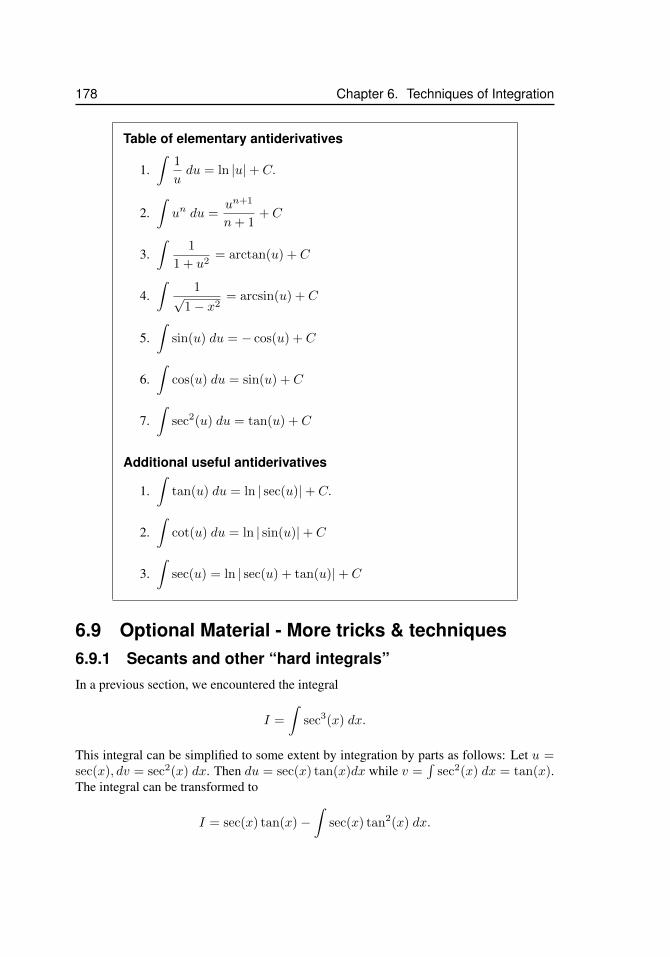
178 Chapter 6. Techniques of Integration
Table of elementary antiderivatives
1.∫
1
udu = ln |u|+ C.
2.∫un du =
un+1
n+ 1+ C
3.∫
1
1 + u2= arctan(u) + C
4.∫
1√1− x2
= arcsin(u) + C
5.∫
sin(u) du = − cos(u) + C
6.∫
cos(u) du = sin(u) + C
7.∫
sec2(u) du = tan(u) + C
Additional useful antiderivatives
1.∫
tan(u) du = ln | sec(u)|+ C.
2.∫
cot(u) du = ln | sin(u)|+ C
3.∫
sec(u) = ln | sec(u) + tan(u)|+ C
6.9 Optional Material - More tricks & techniques6.9.1 Secants and other “hard integrals”In a previous section, we encountered the integral
I =
∫sec3(x) dx.
This integral can be simplified to some extent by integration by parts as follows: Let u =sec(x), dv = sec2(x) dx. Then du = sec(x) tan(x)dx while v =
∫sec2(x) dx = tan(x).
The integral can be transformed to
I = sec(x) tan(x)−∫
sec(x) tan2(x) dx.
6.9. Optional Material - More tricks & techniques 179
The latter can be rewritten:
I1 =
∫sec(x) tan2(x) dx =
∫sec(x)(sec2(x)− 1).
where we have use a trigonometric identity for tan2(x). Then
I = sec(x) tan(x)−∫
sec3(x) dx+
∫sec(x) dx = sec(x) tan(x)− I +
∫sec(x) dx
so (taking both I’s to the left hand side, and dividing by 2)
I =1
2
(sec(x) tan(x) +
∫sec(x) dx
).
We are now in need of an antiderivative for sec(x). No “obvious substitution” or furtherintegration by parts helps here, but it can be checked by differentiation that∫
sec(x) dx = ln | sec(x) + tan(x)|+ C
Then the final result is
I =1
2(sec(x) tan(x) + ln | sec(x) + tan(x)|) + C
6.9.2 A special case of integration by partial fractionsEvaluate this integral25: ∫ 2
1
7x+ 4
6x2 + 7x+ 2dx
This integral involves a rational function (that is, a ratio of two polynomials). The denom-inator is a degree 2 polynomial function that has two roots and that can be factored easily;the numerator is a degree 1 polynomial function. In this case, we can use the followingstrategy. First, factor the denominator:
6x2 + 7x+ 2 = (2x+ 1)(3x+ 2)
Assign A and B in the following way:
A
2x+ 1+
B
3x+ 2=
7x+ 4
(2x+ 1)(3x+ 2)=
7x+ 4
6x2 + 7x+ 2
(Remember, this is how we define A and B.)Next, find the common denominator and rewrite it as a single fraction in terms of A
and B.A
2x+ 1+
B
3x+ 2=
3Ax+ 2A+ 2Bx+B
(2x+ 1)(3x+ 2)
25This section was contributed by Lu Fan
180 Chapter 6. Techniques of Integration
Group like terms in the numerator, and note that this has to match the original fraction, so:
3Ax+ 2A+ 2Bx+B
(2x+ 1)(3x+ 2)=
(3A+ 2B)x+ (2A+B)
(2x+ 1)(3x+ 2)=
7x+ 4
(2x+ 1)(3x+ 2)
The above equation should hold true for all x values; therefore:
3A+ 2B = 7, 2A+B = 4
Solving the system of equations leads to A = 1, B = 2. Using this result, we rewrite theoriginal expression in the form:
7x+ 4
6x2 + 7x+ 2=
7x+ 4
(2x+ 1)(3x+ 2)=
A
2x+ 1+
B
3x+ 2=
1
2x+ 1+
2
3x+ 2
Now we are ready to rewrite the integral:
I =
∫ 2
1
7x+ 4
6x2 + 7x+ 2dx =
∫ 2
1
(1
2x+ 1+
2
3x+ 2
)dx
Simplify:
I =
∫ 2
1
1
2x+ 1dx+ 2
∫ 2
1
1
3x+ 2dx
Now the integral becomes a simple natural log integral that follows the pattern of Eqn. 6.1.Simplify:
I =1
2ln |2x+ 1|
∣∣∣∣21
+2
3ln |3x+ 2|
∣∣∣∣21
.
Simplify further:
I =1
2(ln 5− ln 3) +
2
3(ln 8− ln 5) = −1
6ln 5− 1
2ln 3 +
2
3ln 8.
This method can be used to solve any integral that contain a fraction with a degree 1polynomial in the numerator and a degree 2 polynomial (that has two roots) in the denom-inator.
6.10. Exercises 181
6.10 ExercisesExercise 6.1 Differential Notation The differential of the function y(x) is defined asdy = y′(x)dx, i.e. as the product between y′(x) and the differential of x, dx. For example,given
y(x) = 3x+ sin(2x),
its differential isdy = y′(x)dx = (3 + 2 cos(2x))dx.
Calculate the differentials of the following functions:
(a) f(x) = ex2
(b) f(x) = (x+ 1)2 (c) f(x) =√x
(d) f(x) = arcsin(x) (e) f(x) = x2 + 3x+ 1 (f) f(x) = cos(2x)
(g) y = x6 + 2x4 − 2x (h) y = (x− 2)2(x+ 1)5 (i) y =x
x+ 3
Exercise 6.2 More Differential Notation Given the differential of a function y in termsof the product between its derivative y′(x) and the differential of x, (dx), express the samedifferential in terms of the the differential of y itself, i.e., dy. Then, use the result com-bined with the fundamental theorem of calculus to calculate the corresponding indefiniteintegrals. For example, if we know that the differential of a function y(x) is given by
dy = (3 + 2 sin(2x))dx, (or, equivalently, y(x) =
∫(3 + 2 sin(2x))dx)
we need to figure out that y(x) = 3x− cos(2x) and express the differential given above interms of the differential of y itself
(3 + 2 sin(2x))dx = d(3x− cos(2x)).
Using this result and the fundamental theorem of calculus, we can solve the following∫(3 + 2 sin(2x))dx =
∫d(3x− cos(2x)) = 3x− cos(2x) + C.
(Those marked by a star are a little bit more difficult since they involve composite func-
182 Chapter 6. Techniques of Integration
tions.)
(a) x3 dx =?,
∫x3 dx =? (b) x3/2 dx =?,
∫x3/2 dx =?
(c)1
x3dx =?,
∫1
x3dx =? (d)
√x dx =?,
∫ √x dx =?
(e)1√xdx =?,
∫1√xdx =? (f) e−2x dx =?,
∫e−2x dx =?
(g) (x+ 1)2 dx =?,
∫(x+ 1)2 dx =? (h)
1
(x+ 3)2dx =?,
∫1
(x+ 3)2dx =?
(i) cos(2x) dx =?,
∫cos(2x) dx =? (j) sec2(x) dx =?,
∫sec2(x) dx =?
(k)1
xdx =?,
∫1
xdx =? (l)
1
1 + x2dx =?,
∫1
1 + x2dx =?
(m)∗ 2xex2
dx =?,
∫2xex
2
dx =? (n)∗ 3x2 cos(x3) dx =?,
∫3x2 cos(x3) dx =?
(o)∗2x
1 + x2dx =?,
∫2x
1 + x2dx =? (p)∗
2x
1 + x4dx =?,
∫2x
1 + x4dx =?
Exercise 6.3 Substitutions
(a) Evaluate the following indefinite integrals using the substitution method:
(i) sin(3x) dx (ii)∫
cos(√x)√
xdx
(iii)∫x3√x4 + 1 dx (iv)
∫4
1 + 2xdx
(b) Calculate the following definite integrals using the substitution rule:
(i)∫ 5
0
(√
3 + 2x) dx (ii)∫ π/4
0
sin(4t) dt (iii)∫ √π
0
x cos(x2) dx
Exercise 6.4 More substitutions Compute the following integrals using substitution.
(a)∫ p
1
1
1 + y2dy (b)
∫x2(x3 + 1)6 dx (c)
∫ex√
1 + 2ex dx
(d)∫
1
x ln(x)dx (e)
∫1
1− ydy (f)
∫ S
1
k1
k2 − ndn, k1, k2 > 0
(g)∫
x2
1− x3dx (h)
∫ √3x+ 1 dx (i)
∫x√
4 + x2dx
(j)∫
cos(x) sin5(x) dx (k)∫
3
4 + 5xdx (l)
∫cot(θ) dθ
(m)∫
sec2(x)√2 + tan(x)
dx (n)∫
2
4 + x2dx
6.10. Exercises 183
Exercise 6.5 Trigonometric Substitution The integral∫
sin(x) cos(x)dx can be com-puted in several ways:
(a) using the substitution u = sin(x) (or u = cos(x))
(b) by first using the trigonometric identity sin(2x) = 2 sin(x) cos(x) and then integrating.
Show that the two answers are equivalent. (Hint: you will find that this is a good opportu-nity to review trigonometric identities.)
Exercise 6.6 More Trigonometric substitution The integral∫ 1
0
√1− x2 dx can be
computed using the trigonometric substitution x = sin(u).
(a) Show that this reduces the integral to∫
cos2(u) du.
(b) Use the identity cos2(u) =1 + cos(2u)
2to re-express the integral in a simpler form.
Then integrate.
(c) Explain why the answer is the same as the area of 1/4 of a circle of radius 1.
Exercise 6.7 Partial Fractions Compute the following integrals. Use factoring and/orcompleting the square and partial fractions, or some other technique if necessary.
(a)∫
1
x2 − x− 20dx (b)
∫3
x2 + 6x+ 9dx
(c)∫
−1
x2 + 4x+ 14dx (d)
∫2
x2 − 6x+ 8dx
Exercise 6.8 More Partial Fractions The two integrals shown below may look verysimilar, but in fact they lead to quite different results:
(a)∫
dx
a2 + x2(b)
∫dx
a2 − x2
(Hint: (a) can be reduced to an inverse tangent type integral by a bit of algebraic rearrange-ment and a substitution of the form u = x/a and (b) can be integrated by factoring theexpression a2 − x2 and using the method of partial fractions.)
Exercise 6.9 Integration by Parts Use integration by parts to show that∫xnexdx =
xnex − n∫xn−1exdx
Exercise 6.10 More Integration by Parts First make a substitution and then use integra-
184 Chapter 6. Techniques of Integration
tion by parts to evaluate the following integrals:
(a)∫
sin(√x) dx (b)
∫ 4
1
e√x dx
(c)∫ √π√π/2
x3 cos(x2)dx (d)
∫x5ex
2
dx
Exercise 6.11 Compute the following integrals.
(a)∫
3
x2 + 4x+ 6dx (b)
∫2
(x+ 1)(x+ 2)dx (c)
∫1
x2 + 6x+ 8dx
(d)∫ p
1
1
1− y2dy (e)
∫ T
0
te−2t dt (f)∫ π
0
x sin(x
2
)dx
(g)∫
x2 ln(x) dx
Exercise 6.12 Integration drills Note: some simplifications in a few of these will make
6.10. Exercises 185
your work much easier.
(1)∫
1
xlnx dx (2)
∫2
2 + 3xdx
(3)∫
x2 sin(3x3 + 1
)dx (4)
∫ 2
1
2t e3t2 dt
(5)∫ 1
0
x
1 + x2dx (6)
∫1√
2− 3x2dx
(7)∫
2
3 + 4x2dx (8)
∫1√
25− 4x2dx
(9)∫
x1√
9 + x2dx (10)
∫cos(3x)(1− sin(3x)) dx
(11)∫
cos(2x)(1− sin(2x)) dx (12)∫
sec2(x)√
tan(x) + 1 dx
(13)∫ π/2
0
(1− sin2(t)) sin(t) dt (14)∫
2x(1− sin(2x)) dx
(15)∫
sec(x) tan(x) dx
(Hint: use trig identities)
(16)∫
x sin(x+ 1) dx
(17)∫
(x sin2(x) + x cos2(x))5 dx
(Hint: look carefully!)
(18)∫
sec2(t) dt
(19)∫
1
2x2 + 12x+ 18dx
(Hint: some algebra, please)
(20)∫
1
(x− 5)(x+ 1)dx
(21)∫
1
(x+ 3)(2x− 1)dx (22)
∫1
(x+ 2)(x+ 3)dx
(23)∫
3x2 + 1
x2(x2 + 1)2dx (24)
∫1
x2 − 3x+ 2dx
(Hint: try factoring)
(25)∫
3
x2 + 3x+ 15dx (26)
∫x sec2(x) dx
(27)∫
xex2
dx (28)∫
x2ex dx
(29)∫
arctan(x) dx (30)∫
x cos(x)ex dx
Exercise 6.13 Consider the curve y = f(x) =√
1− x2 (which is a part of a circleof radius 1) over the interval 0 < x < 1. Suppose this curve is rotated about the yaxis to generate the top half of a sphere. Set up an integral which computes the volumeof this hemisphere using the shell method, and compute the volume. (You will need tomake a substitution to simplify the integral. To do this question, some techniques of anti-differentiation are required.)
186 Chapter 6. Techniques of Integration
Exercise 6.14 Let the density of mass along a bar of length L be given by p(x) = e−ax.
(a) Find the total mass of the bar.
(b) Find the average mass density along the bar.
(c) Find the center of mass of the bar.
Exercise 6.15 Find the center of mass of a distribution p(x) = sin(2x) for 0 < x < π2 .
Exercise 6.16 Bacteria are grown in a 1-dimensional tube. The mass density of thebacteria per unit distance along the tube is given by the function b(x) = β
√a2 − x2 for
0 < x < a.
(a) Find the total mass of bacteria in the tube.
(b) Find the center of mass of the bacteria.
Exercise 6.17 Gel electrophoresis is an experimental technique used in molecular biologyto separate proteins (or other molecules) according to their molecular weights and charges.Suppose that in such an experiment, the distribution of protein along a 1-dimensional stripof this gel is found to be p(x) = xe−x/2 where 0 ≤ x ≤ 5 is distance in cm from the endof the strip and p(x), is the density of the protein per unit distance (in arbitrary units).
(a) Sketch a graph of this distribution.
(b) Determine the location x = xc where the density of the protein is greatest. (Indicateon the graph and find using calculus.)
(c) Find the total amount of protein in the region xc − 1 ≤ x ≤ xc + 1.
(d) Find the mean (center of mass) of the distribution, i.e. the average x coordinate of theprotein distribution.
Exercise 6.18 Find the length of the curve y = f(x) = x3/2 for 0 < x < 1. (To do thisquestion, some techniques of anti-differentiation are required.)
Exercise 6.19 To do this question, some techniques of anti-differentiation are required.
(a) Use the chain rule to show that F ′(x) = sec(x) is the derivative of the function F (x) =ln(sec(x) + tan(x)). Therefore, what is the anti-derivative of f(x) = sec(x)?
(b) Use integration by parts to show that∫sec3(x)dx =
1
2(sec(x) tan(x) + ln(sec(x) + tan(x)) + C.
(Hint: recall the trigonometric identity 1 + tan2(x) = sec2(x)).
(c) Set up an integral to compute the arc-length of the curve y = x2/2 for 0 < x < 1.
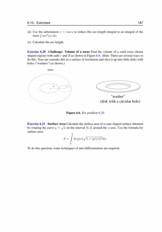
6.10. Exercises 187
(d) Use the substitution x = tanu to reduce this arc-length integral to an integral of theform
∫sec3(u) du.
(e) Calculate the arc-length.
Exercise 6.20 Challenge: Volume of a torus Find the volume of a solid torus (donutshaped region) with radii r and R as shown in Figure 6.6. (Hint: There are several ways todo this. You can consider this as a surface of revolution and slice it up into little disks withholes (“washers”) as shown.)
Rr
torus
"washer"
(disk with a circular hole)
Figure 6.6. For problem 6.20
Exercise 6.21 Surface Area Calculate the surface area of a cone shaped surface obtainedby rotating the curve y =
√x on the interval [0, 2] around the x-axis. Use the formula for
surface area:
S =
2∫0
2πy(x)√
1 + (y′(x))2dx.
To do this question, some techniques of anti-differentiation are required.

188 Chapter 6. Techniques of Integration
Chapter 7
Improper integrals
7.1 IntroductionThe goal of this chapter is to meaningfully extend our theory of integrals to improperintegrals. There are two types of so-called improper integrals: the first involves integratinga function over an infinite domain and the second involves integrands that are undefined atpoints within the domain of integration. In order to integrate over an infinite domain, weconsider limits of the form limb→∞
∫ baf(x)dx. If the integrand is not defined at c (a < c <
b) then we split the integral and consider the limits∫ baf(x)dx = limε→0
∫ c−εa
f(x)dx +
limε→0
∫ bc+ε
f(x)dx. The latter is sometimes also referred to as improper integrals of thesecond kind. Such situations occur, for example, for rational functions f(x) = p(x)/q(x)whenever q(x) has zeroes in the domain of integration.
The notions of convergence and divergence as discussed in Chapter 10 & 11 in thecontext of sequences and series will be very important to determine these limits. Improperintegrals (of both types) arise frequently in applications and in probability. By relatingimproper integrals to infinite series we derive the last convergence test: the Integral Com-parison test. As an application we finally prove that the p-series
∑∞k=1 k
−p converges forp > 1 and diverges otherwise.
7.2 Integration over an infinite domainWe will see that there is a close connection between certain infinite series and improperintegrals, which involve integrals over an infinite domain. We have already encounteredexamples of improper integrals in Section 3.8 and in the context of radioactive decay inSection 8.4. Recall the following definition:
Definition 1 (Improper integral (first kind)). An improper integral of the first kind is anintegral performed over an infinite domain, e.g.∫ ∞
a
f(x) dx.
189
190 Chapter 7. Improper integrals
The value of such an integral is understood to be a limit, as given in the following definition:
∫ ∞a
f(x) dx = limb→∞
∫ b
a
f(x) dx.
We evaluate an improper integral by first computing a definite integral over a finitedomain a ≤ x ≤ b, and then taking a limit as the endpoint b moves off to larger and largervalues. The definite integral can be interpreted as an area under the graph of the function.The essential question being addressed here is whether that area remains bounded when weinclude the “infinite tail” of the function (i.e. as the endpoint b moves to larger values.) Forsome functions (whose values get small enough, fast enough) the answer is “yes”.
Definition 2 (Convergence). If the limit
limb→∞
∫ b
a
f(x) dx
exists, we say that the improper integral converges. Otherwise we say that the improperintegral diverges.
With these definitions in mind, we can compute a number of classic integrals.
7.2.1 Example: Decaying exponentialRecall that the improper integral of a decaying exponential converges – we have seen thisearlier, in Section 3.8.5, and again in applications in Sections 7.3 and 8.4.1. Here werecapitulate this important result in the context of improper integrals. Suppose that r > 0and let
I =
∫ ∞0
e−rt dt ≡ limb→∞
∫ b
0
e−rt dt.
Then
I = limb→∞
−1
re−rt
∣∣∣∣b0
= −1
rlimb→∞
(e−rb − e0) = −1
r( limb→∞
e−rb︸ ︷︷ ︸0
−1) =1
r,
where we have used the fact that limb→∞ e−rb = 0 for r > 0. Thus the limit exists (isfinite) and hence the integral converges. More precisely, it converges to the value I = 1/r.
7.2.2 Example: The improper integral of 1/x divergesWe now consider a classic and counter-intuitive result, and one of the most important resultsin this chapter. Consider the function
y = f(x) =1
x.
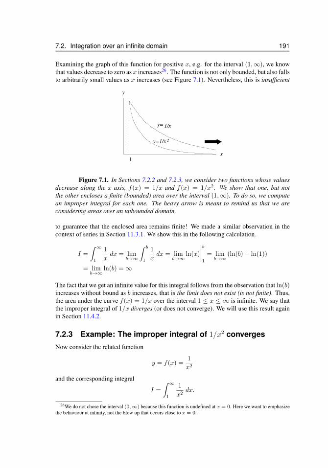
7.2. Integration over an infinite domain 191
Examining the graph of this function for positive x, e.g. for the interval (1,∞), we knowthat values decrease to zero as x increases26. The function is not only bounded, but also fallsto arbitrarily small values as x increases (see Figure 7.1). Nevertheless, this is insufficient
1
x
y
y= 1/x
y=1/x 2
Figure 7.1. In Sections 7.2.2 and 7.2.3, we consider two functions whose valuesdecrease along the x axis, f(x) = 1/x and f(x) = 1/x2. We show that one, but notthe other encloses a finite (bounded) area over the interval (1,∞). To do so, we computean improper integral for each one. The heavy arrow is meant to remind us that we areconsidering areas over an unbounded domain.
to guarantee that the enclosed area remains finite! We made a similar observation in thecontext of series in Section 11.3.1. We show this in the following calculation.
I =
∫ ∞1
1
xdx = lim
b→∞
∫ b
1
1
xdx = lim
b→∞ln(x)
∣∣∣∣b1
= limb→∞
(ln(b)− ln(1))
= limb→∞
ln(b) =∞
The fact that we get an infinite value for this integral follows from the observation that ln(b)increases without bound as b increases, that is the limit does not exist (is not finite). Thus,the area under the curve f(x) = 1/x over the interval 1 ≤ x ≤ ∞ is infinite. We say thatthe improper integral of 1/x diverges (or does not converge). We will use this result againin Section 11.4.2.
7.2.3 Example: The improper integral of 1/x2 convergesNow consider the related function
y = f(x) =1
x2
and the corresponding integral
I =
∫ ∞1
1
x2dx.
26We do not chose the interval (0,∞) because this function is undefined at x = 0. Here we want to emphasizethe behaviour at infinity, not the blow up that occurs close to x = 0.
192 Chapter 7. Improper integrals
Then
I = limb→∞
∫ b
1
x−2 dx = limb→∞
(−x−1)
∣∣∣∣b1
= − limb→∞
(1
b− 1
)= 1.
Thus, the limit exists, and is I = 1. In contrast to the example in Section 7.2.2, this integralconverges.
We observe that the behaviours of the improper integrals of the functions 1/x and1/x2 are very different. The former diverges, while the latter converges. The only differ-ence between these functions is the power of x. As shown in Figure 7.1, that power affectshow rapidly the graph “falls off” to zero as x increases. The function 1/x2 decreases muchfaster than 1/x. Consequently 1/x2 has a sufficiently “slim” infinite “tail”, such that thearea under its graph does not become infinite - not an easy concept to digest! This observa-tions leads us to wonder what power p is needed to make the improper integral of a function1/xp converge. We answer this question below.
7.2.4 When does the integral of 1/xp converge?Here we consider an arbitrary power, p, that can be any real number. We ask when thecorresponding improper integral converges or diverges. Let
I =
∫ ∞1
1
xpdx.
For p = 1 we have already established that this integral diverges (see Section 7.2.2), andfor p = 2 we have seen that it is convergent (see Section 7.2.3). By a similar calculation,we find that
I = limb→∞
x1−p
(1− p)
∣∣∣∣b1
= limb→∞
(1
1− p
)(b1−p − 1
).
Thus, this integral converges provided that the term b1−p does not “blow up” as b increases.For this to be true, we require that the exponent (1− p) should be negative, i.e. 1− p < 0or p > 1. In this case, we have
I =1
p− 1.
To summarize our result,
∫ ∞1
1
xpdx converges if p > 1, and diverges if p ≤ 1.
Examples:
(i) The integral ∫ ∞1
1√xdx, diverges.
We see this from the following argument:√x = x
12 , so p = 1
2 < 1. Thus, by thegeneral result, this integral diverges.
7.3. Application: Present value of a continuous income stream 193
(ii) The integral ∫ ∞1
x−1.01 dx, converges.
Here p = 1.01 > 1, so the result implies convergence of the integral.
7.3 Application: Present value of a continuousincome stream
Here we discuss the value of an annuity, which is a kind of savings account that guaranteesa continuous stream of income. You would like to pay P dollars to purchase an annuity thatwill pay you an income f(t) every year from now on, for t > 0. In some cases, we mightwant a constant income every year, in which case f(t) would be constant. More generally,we can consider the case that at each future year t, we ask for income f(t) that could varyfrom year to year. If the bank interest rate is r, how much should you pay now?
Solution
If we invest P dollars (the “principal” i.e., the amount deposited) in the bank with interestr then the amount A(t) in the account at time t (in years), will grow as follows:
A(t) = P(
1 +r
n
)nt,
where r is the annual interest rate (e.g. 5%) and n is the number of times per year thatinterest is compound (e.g. n = 2 means interest compounded twice per year, n = 12means monthly compounded interest, etc.). Define h = r
n . Then at time t, we have that
A(t) = P (1 + h)1h rt
= P[(1 + h)
1h
]rt≈ Pert for large n or small h.
Here we have used the fact that when h is small (i.e. frequent intervals of compounding)the expression in square brackets above can be approximated by e, the base of the naturallogarithms. Recall that
e = limh→0
[(1 + h)
1h
].
This result was obtained in a first semester calculus course by selecting the base of expo-nentials such that the derivative of ex is just ex itself. Thus, we have found that the amountin the bank at time t will grow as
A(t) = Pert, continually compounded interest. (7.1)
Having established the exponential growth of an investment, we return to the questionof how to set up an annuity for a continuous stream of income in the future. Rewriting
194 Chapter 7. Improper integrals
Eqn. (7.1), the principle amount that we should invest in order to have A(t) to spend attime t is
P = A(t)e−rt.
Suppose we want to have f(t) spending money for each year t. We refer to the presentvalue of year t as the quantity
P = f(t)e−rt,
i.e. we must pay P now, in the present, to get f(t) in a future year t. Summing over all theyears, we find that the present value of the continuous income stream is
P =
L∑t=1
f(t)e−rt · 1︸︷︷︸“∆t”
≈∫ L
0
f(t)e−rt dt,
where L is the expected number of years left in the lifespan of the individual to whom thisannuity will be paid, and where we have approximated a sum of payments by an integral(of a continuous income stream). One problem is that we do not know in advance how longthe lifespan L will be. As a crude approximation, we could assume that this income streamcontinues forever, i.e. that L ≈ ∞. In such an approximation, we have to compute theintegral:
P =
∫ ∞0
f(t)e−rt dt. (7.2)
The integral in Eqn. (7.2) is an improper integral (i.e. integral over an unbounded do-main), as we have already encountered in Section 3.8.5. We shall have more to say aboutthe properties of such integrals, and about their technical definition, existence, and proper-ties in Chapter 7. We refer to the quantity
P =
∫ ∞0
f(t)e−rt dt, (7.3)
as the present value of a continuous income stream f(t).
Example: Setting up an annuity
Suppose we want an annuity that provides us with an annual payment of 10, 000 from thebank, i.e. in this case f(t) = $10, 000 is a function that has a constant value for every year.Then from Eqn (7.3),
P =
∫ ∞0
10000e−rt dt = 10000
∫ ∞0
e−rt dt.
By a previous calculation in Section 3.8.5, we find that
P = 10000 · 1
r,
e.g. if interest rate is 5% (and assumed constant over future years), then
P =10000
0.05= $200, 000.
Therefore, we need to pay $200,000 today to get 10, 000 annually for every future year.
7.4. Integral comparison test 195
7.4 Integral comparison testThe integrals discussed above can be used to make comparisons that help us to identifywhen other improper integrals converge or diverge27. The following important result estab-lishes how these comparisons work:
Suppose we are given two functions, f(x) and g(x), both continuous on someinfinite interval [a,∞). Suppose, moreover, that at all points on this intervalthe first function is smaller than the second, i.e.
0 ≤ f(x) ≤ g(x).
Then the following conclusions can be made:a
(i)∫ ∞a
f(x) dx ≤∫ ∞a
g(x) dx.
The area under f(x) is smaller than the area under g(x).
(ii) If∫ ∞a
g(x) dx converges, then∫ ∞a
f(x) dx converges.
If the larger area is finite, so is the smaller one.
(iii) If∫ ∞a
f(x) dx diverges, then∫ ∞a
g(x) dx diverges.
If the smaller area is infinite, so is the larger one.aThese statements have to be carefully noted. What is assumed and what is concluded works
“one way”. That is the order “if . . . then” is important. Reversing that order leads to a commonerror.
Example: Determine whether the following integral converges:∫ ∞1
x
1 + x3dx.
Solution: by noting that for all x > 0
0 ≤ x
1 + x3≤ x
x3=
1
x2.
Note that for x > 0
0 ≤ x
1 + x3≤ x
x3=
1
x2.
Thus, ∫ ∞1
x
1 + x3dx ≤
∫ ∞1
1
x2dx.
Since the larger integral on the right is known to converge, so does the smaller integral onthe left. ♦
27Similar ideas will be employed for the comparison of infinite series in Chapter 11. A recurring theme in thiscourse is the close connection between series and integrals, for example, recall the Riemann sums in Chapter 2.
196 Chapter 7. Improper integrals
7.5 Integration of an unbounded integrandThe second kind of improper integrals refers to integrands that are undefined at one (ormore) points of the domain of integration [a, b]. Suppose f(x) is continuous on the openinterval (a, b) but becomes infinite at the lower bound, x = a. Then the integral of f(x)over the domain [a+ ε, b] for ε > 0 has a definite value regardless of how small ε is chosen.Therefore, we can consider the limit
limε→0+
∫ b
a+ε
f(x)dx,
where ε → 0+ means that ε approaches 0 from ‘above’, i.e. ε > 0 always holds. If thislimit exists and is equal to L, then we define∫ b
a
f(x)dx = L.
If an anti-derivative of f(x), say F (x) is known, then the fundamental theorem of calculuspermits us to compute ∫ b
a+ε
f(x)dx = F (b)− F (a+ ε).
We are thus led to determine the existence (or nonexistence) of the limit
limε→0+
F (a+ ε).
Example 1: Calculate the following integral for p 6= 1:
I =
∫ b
a
dx
(x− a)p.
Solution: We interpret the integral as the following limit:
I = limε→0+
∫ b
a+ε
dx
(x− a)p= − lim
ε→0+
1
p− 1
[1
(b− a)p−1− 1
εp−1
].
Thus, for p > 1 the term ε1−p becomes arbitrarily large as ε → 0+ and hence the areadiverges and the integral does not exist. Conversely, for p < 1 the term ε1−p converges to0 as ε→ 0+ and hence the improper integral exists and is
I =(b− a)1−p
1− p.
Finally, note that for p = 1 the anti-derivative is undefined and the integral does not exist.Alternatively, for p = 1 we directly see that∫ b
a+ε
dx
x− a= ln
(b− aε
)
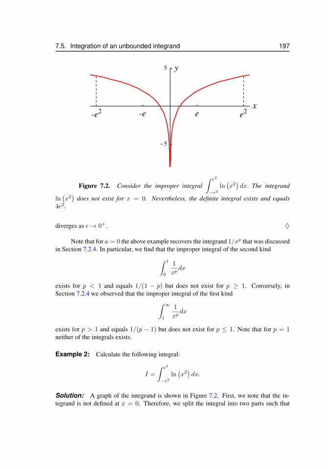
7.5. Integration of an unbounded integrand 197
!e2 !e e e2
!5
5
x
y
e-e2 e2-e
Figure 7.2. Consider the improper integral∫ e2
−e2ln(x2)dx. The integrand
ln(x2)
does not exist for x = 0. Nevertheless, the definite integral exists and equals4e2.
diverges as ε→ 0+. ♦
Note that for a = 0 the above example recovers the integrand 1/xp that was discussedin Section 7.2.4. In particular, we find that the improper integral of the second kind∫ 1
0
1
xpdx
exists for p < 1 and equals 1/(1 − p) but does not exist for p ≥ 1. Conversely, inSection 7.2.4 we observed that the improper integral of the first kind∫ ∞
1
1
xpdx
exists for p > 1 and equals 1/(p − 1) but does not exist for p ≤ 1. Note that for p = 1neither of the integrals exists.
Example 2: Calculate the following integral:
I =
∫ e2
−e2ln(x2)dx.
Solution: A graph of the integrand is shown in Figure 7.2. First, we note that the in-tegrand is not defined at x = 0. Therefore, we split the integral into two parts such that
198 Chapter 7. Improper integrals
the undefined point marks once the upper and once the lower bound and we write the twointegrals as a limit:
I =
∫ e2
−e2ln(x2)dx = lim
ε→0−
∫ ε
−e2ln(x2)dx+ lim
ε→0+
∫ e2
ε
ln(x2)dx,
where ε → 0− means ε approaches 0 from below, i.e. ε < 0 always holds. Second, theintegrand is an even function and the integral runs over a symmetric domain. Hence we get
I = limε→0+
2
∫ e2
ε
ln(x2)dx.
The integral can be solved using the substitution u = x2 followed by an integration byparts. This yields
Check it!
I = limε→0+
2x(ln(x2)− 2)∣∣∣∣e2ε
= 4 limε→0+
x (ln(x)− 1)
∣∣∣∣e2ε
= 4e2 − limε→0+
ε(ln(ε)− 1).
The fact that the limit exists and converges to 0 can be seen by setting ε = 1/k and consid-ering the limit k →∞:
limε→0+
ε(ln(ε)− 1) = limk→∞
1
k(ln(
1
k)− 1) = − lim
k→∞
1
k(ln(k) + 1).
Now we can use either de l’Hopital’s rule or simply recognize that k grows much fasterthan ln k and hence the limit converges to 0. Thus, we find that the improper integral existsand is
I = 4e2.
♦
7.6 L’Hopital’s ruleThis section introduces a powerful method to evaluate tricky limits of the form limx→a
f(x)g(x) .
The rule is named after the French mathematician Guillaume de l’Hopital, who publishedit in the 17th century. For our purposes, the rule is often particularly useful to evaluatethe limits that arise in improper integrals of the first (unbounded domain) and second kind(unbounded integrand).
Consider two functions, f(x) and g(x), and suppose that the following four prereq-uisites are satisfied:
(a) f(x) and g(x) are differentiable near x = a, but not necessarily at x = a.
(b) g′(x) 6= 0 for x near a but x 6= a.
(c) limx→a
f ′(x)
g′(x)exists.
7.6. L’Hopital’s rule 199
(d) and either
(i) limx→a
f(x) = limx→a
g(x) = 0, or
(ii) limx→a
f(x) = ±∞, limx→a
g(x) = ±∞.
Then, l’Hopital’s rule states that
limx→a
f(x)
g(x)= limx→a
f ′(x)
g′(x). (7.4)
Note: values of the limit a can include ±∞.
In loose terms, l’Hopital’s rule can be used if
limx→a
f(x)
g(x)is of type
0
0or ± ∞
∞.
Let us now explore the power of l’Hopital’s rule through several examples.
Example 1: Calculate the following limit:
limx→0
sinx
ex − 1.
Solution: In this example l’Hopital’s rule can be used because limx→0 sinx = 0 andlimx→0(ex − 1) = 0. Thus,
limx→0
sinx
ex − 1= lim
x→0
(sinx)′
(ex − 1)′= limx→0
cosx
ex
=limx→0
cosx
limx→0
ex(because of non-zero denominator)
=cos 0
1= 1.
♦
Example 2: Calculate the following limit:
limt→∞
t ln t
t2 + 1.
200 Chapter 7. Improper integrals
Solution: In this example, we can use l’Hopital’s rule because both the numerator andthe denominator diverge: limt→∞(t ln t) =∞ and limt→∞(t2 + 1) =∞. Thus,
limt→∞
t ln t
t2 + 1= lim
t→∞
(t ln t)′
(t2 + 1)′= limt→∞
ln t+ 1
2t.
Unfortunately, the new limit that results from applying l’Hopital’s rule remains tricky.However, we can simply apply l’Hopital’s rule again because the prerequisites are stillsatisfied. In this case, the numerator and denominator still diverge: limt→∞(ln t+ 1) =∞and limt→∞ 2t =∞. Using l’Hopital’s rule again, we obtain
limt→∞
ln t+ 1
2t= lim
t→∞
(ln t+ 1)′
(2t)′= limt→∞
1t
2=
limt→∞
1
t2
= 0.
Note: As long as all prerequisites of l’Hopital’s rule remain satisfied, the rule can be appliedrepeatedly. ♦
Example 3: Calculate the following limit:
limx→0+
sinx
x2.
Note: a plus-sign (+) added to the limit means that x approaches the limit from above (orfrom the right). In the present case, x > 0 always holds as x approaches zero. Later in thisexample we will see why this subtle point is important. In analogy, a minus-sign (−) addedto the limit means that the limit is approached from below (or from the left). If no sign isadded, it does not matter whether the limit is approached from above, below or even in analternating manner.
Solution: Again, l’Hopital’s rule can be used because limx→0 sinx = 0 and limx→0 x2 =
0. Thus,
limx→0+
sinx
x2= lim
x→0+
(sinx)′
(x2)′= limx→0+
cosx
2x.
In order to evaluate this new limit, we might be tempted to apply l’Hopital’s rule again. Isthis permissible? Stop for a moment and think about why or why not.
Check it! Of course, it is not permissible because the numerator limx→0+ cosx = 1 andhence violates the prerequisites for applying l’Hopital’s rule. Ignoring the prerequisitesand blindly applying l’Hopital’s rule again would yield an incorrect limit of zero. Instead,we get
limx→0+
cosx
2x= lim
x→0+cosx · lim
x→0+
1
2x= +∞.
Hence, the limit does not exist, it diverges to +∞.In order to see why it was important to approach the limit from above, x → 0+,
calculate the limit as x approaches zero from below:Check it!
7.7. Summary 201
limx→0−
sinx
x2.
In contrast to the above result, the limit is now −∞ because x < 0 always holds as xapproaches zero. ♦
Example 4: Calculate the following limit:
lima→0+
a ln a.
Note: The limit of zero can only be approached from above, a → 0+, because ln a isundefined for a < 0.
Solution: At first, this limit does not seem to have the correct form to apply l’Hopital’srule. However, we can use a neat little trick and rewrite the limit as a quotient of twofunctions:
lima→0+
a ln a = lima→0+
ln a1a
.
Once rewritten, it becomes apparent that l’Hopital’s rule can indeed be applied becauseagain both the numerator and the denominator diverge: lima→0+ ln a = −∞ and lima→0+ 1/a =∞. Thus,
lima→0+
ln a1a
= lima→0+
(ln a)′
( 1a )′
= lima→0+
1a
− 1a2
= lima→0+
(−a) = 0.
♦
7.7 SummaryThe main points of this chapter can be summarized as follows:
1. We reviewed the definition of an improper integral (type one) over an infinite domain:∫ ∞a
f(x) dx = limb→∞
∫ b
a
f(x) dx.
2. We computed some examples of improper integrals and discussed their convergenceor divergence. We recalled (from earlier chapters) that
I =
∫ ∞0
e−rt dt converges,
whereas
I =
∫ ∞1
1
xdx diverges.
202 Chapter 7. Improper integrals
3. More generally, we showed that∫ ∞1
1
xpdx converges if p > 1, diverges if p ≤ 1.
4. We reviewed the definition of improper integrals (type two) for integrands that areunbounded at either end of the domain of integration, say x = a:∫ b
a
f(x) dx = limε→0
∫ b
a+ε
f(x) dx.
5. If the integrand is not defined at one (or more) point(s) in the interior of the domainof integration, then the integral is split into two (or more) parts and we proceed asabove.
6. In particular, we showed that∫ 1
0
1
xpdx converges if p < 1, diverges if p ≥ 1.
7. L’Hopital’s rule is a powerful tool to evaluate tricky limits that may arise for improperintegrals of both kinds. It states that
limx→a
f(x)
g(x)= limx→a
f ′(x)
g′(x)
if f(a) = g(a) = 0 or limx→a f(x) = limx→a g(x) = ±∞ as well as some, moresubtle prerequisites.
7.8. Exercises 203
7.8 ExercisesExercise 7.1 Consider the integral
A =
∫ D
1
1
xpdx
(a) Sketch a region in the plane whose area represents this if (i) p > 1 and (ii) p < 1.
(b) Evaluate the integral for p 6= 1.
(c) How does the areaA depend on the value ofD in each of the cases (i) and (ii). Does thearea increase without bound asD increases? Or does the area approach some constant?
(d) With this in mind, how might we try to understand an integral of the form∫ ∞1
1
xpdx
Exercise 7.2 Which of the following improper integrals converge? Give a reason in eachcase.
(a)∫ ∞
1
1
x1.001dx (b)
∫ ∞1
x dx (c)∫ ∞
1
x−3 dx
(d)∫ ∞
0
ex dx (e)∫ ∞
0
e−2x dx (f)∫ ∞
0
x e−x dx
Exercise 7.3 The gravitational force between two objects of mass m1 and m2 is F =Gm1m2/r
2 where r is the distance of separation. Initially the objects are a distance Dapart. The work done in moving an object from position D to position x against a force Fis defined as
W =
∫ x
D
F (r) dr.
Find the total work needed to move one of these objects infinitely far away.
Exercise 7.4 “Gabriel’s Horn” is the surface of revolution formed by rotating the graphof the function y = f(x) = 1/x about the x axis for 1 ≤ x <∞.
(a) Find the volume of air inside this shape and show that it is finite.
(b) When we cut a cross-section of this horn along the x−y-plane, we see a flat area whichis wedged between the curves y = 1/x and y = −1/x. Show that this “cross-sectionalarea” is infinite.
(c) The surface area of a surface of revolution generated by revolving the function y =f(x) for a ≤ x ≤ b about the x-axis is given by
S =
∫ b
a
2πf(x)√
1 + (f ′(x))2 dx
Write down an integral that would represent the surface area of “Gabriel’s Horn”.
204 Chapter 7. Improper integrals
(d) The integral in part (c) is not easy to evaluate explicitly – i.e. we cannot find an anti-derivative. However, we can show that it diverges. Set up a comparison that shows thatthe surface area of Gabriel’s horn is infinite.
Exercise 7.5 Does the integral∫ ∞
0
sin (x)
x4 + x2 + 1dx converge or diverge?
Exercise 7.6 Suppose that an airborne disease is introduced into a large population attime t = 0. At time t > 0, the rate at which this disease is spreading is r (t) = 4000te−4t
new infections per day.
(a) After how long is this disease most infectious?
(b) How many people in total acquire the disease?
(c) What eventually happens to the rate of new infections?
Exercise 7.7 Does the integral∫ 5
0
x− 1
x2 + x− 2dx converge or diverge?
Exercise 7.8 Suppose that you place $1,000,000 in an account that earns 5% annualinterest, and you wish to withdraw z dollars from this account one year from now, 2zdollars two years from now, 3z dollars three years from now, and so on. What is themaximum value of z so that you never run out of money?
Exercise 7.9 For which values of p does the integral∫ ∞
2
1
x (lnx)p dx converge?
Exercise 7.10 Evaluate the following limits:
(a) limx→−∞
xe4x (b) limx→∞
x sin
(1
x
)(c) lim
θ→π2
cos (θ)π2 − θ
Exercise 7.11 Determine the convergence of the following integrals. If they converge,find their values:
(a)∫ ∞
0
xe−x dx (b)∫ 1
0
2x√1− x2
dx (c)∫ 1
0
1
1− x3dx
Exercise 7.12 Convergence of an integral of the form∫ ∞−∞
f (x) dx is determined by
splitting the integral up into two parts:∫ ∞−∞
f (x) dx =
∫ 0
−∞f (x) dx+
∫ ∞0
f (x) dx.

7.8. Exercises 205
The integral∫ ∞−∞
f (x) dx is said to converge if both of these two integrals converge. Can
you come up with an example of a function f (x) for which
limb→∞
∫ b
−bf (x) dx <∞
but the integral∫ ∞−∞
f (x) dx diverges?
Exercise 7.13 Evaluate the integral∫ π
0
cos θ√1− sin3 θ
dθ.
Exercise 7.14 Evaluate the integral∫ ∞
0
e−x sinx dx.

206 Chapter 7. Improper integrals
Chapter 8
Continuous probabilitydistributions
8.1 IntroductionWe begin by extending the idea of a discrete random variable28 to the continuous case.We call x a continuous random variable in a ≤ x ≤ b if x can take on any value in thisinterval. An example of a random variable is the height of a person, say an adult male,selected randomly from a population. (This height typically takes on values in the range0.5 ≤ x ≤ 3 meters, say, so a = 0.5 and b = 3.)
If we select a male subject at random from a large population, and measure his height,we might expect to get a result in the proximity of 1.7-1.8 meters most often - thus, suchheights will be associated with a larger value of probability than heights in some otherinterval of equal length, e.g. heights in the range 2.7 < x < 2.8 meters, say. Unlike thecase of discrete probability, however, the measured height can take on any real numberwithin the interval of interest.
8.2 Basic definitions and propertiesCompared to discrete probability, one of the most important differences is that we now con-sider a probability density, rather than a value of the probability per se. First and foremost,we observe that now p(x) will no longer be a probability, but rather “ a probability perunit x”. This idea is analogous to the connection between the mass of discrete beads and acontinuous mass density, encountered previously in Chapter 5.
Definition
A function p(x) is a probability density provided it satisfies the following properties:
1. p(x) ≥ 0 for all x.
2.∫ bap(x) dx = 1 where the possible range of values of x is a ≤ x ≤ b.
28see Math 102.
207
208 Chapter 8. Continuous probability distributions
The probability that a random variable x takes on values in the interval a1 ≤ x ≤ a2
is defined as
∫ a2
a1
p(x) dx.
The transition to probability density means that the quantity p(x) does not carry the samemeaning as our previous notation for probability of an outcome xi, namely p(xi) in thediscrete case. In fact, p(x)dx, or its approximation p(x)∆x is now associated with theprobability of an outcome whose values is “close to x”.
Unlike our previous discrete probability, we will not ask “what is the probability thatx takes on some exact value?” Rather, we ask for the probability that x is within somerange of values, and this is computed by performing an integral29.
Having generalized the idea of probability, we will now find that many of the asso-ciated concepts have a natural and straight-forward generalization as well. We first definethe cumulative function, and then show how the mean, median, and variance of a contin-uous probability density can be computed. Here we will have the opportunity to practiceintegration skills, as integrals replace the sums in such calculations.
Definition
For experiments whose outcome takes on values on some interval a ≤ x ≤ b, we define acumulative function, F (x), as follows:
F (x) =
∫ x
a
p(s) ds.
Then F (x) represents the probability that the random variable takes on a value in the range(a, x) 30. The cumulative function is simply the area under the probability density (betweenthe left endpoint of the interval, a, and the point x).
The above definition has several implications:
Properties of continuous probability
1. Since p(x) ≥ 0, the cumulative function is an increasing function.
2. The connection between the probability density and its cumulative function can bewritten (using the Fundamental Theorem of Calculus) as
p(x) = F ′(x).
29Remark: the probability that x is exactly equal to b is the integral∫ b
bp(x) dx. But this integral has a value
zero, by properties of the definite integral.30By now, the reader should be comfortable with the use of “s” as the “dummy variable” in this formula, where
x plays the role of right endpoint of the interval of integration.
8.2. Basic definitions and properties 209
3. F (a) = 0. This follows from the fact that
F (a) =
∫ a
a
p(s) ds.
By a property of the definite integral, this is zero.
4. F (b) = 1. This follows from the fact that
F (b) =
∫ b
a
p(s) ds = 1
by Property 2 of the definition of the probability density, p(x).
5. The probability that x takes on a value in the interval a1 ≤ x ≤ a2 is the same as
F (a2)− F (a1).
This follows from the additive property of integrals and the Fundamental Theoremof Calculus:∫ a2
a
p(s) ds−∫ a1
a
p(s) ds =
∫ a2
a1
p(s) ds =
∫ a2
a1
F ′(s) ds = F (a2)− F (a1)
Finding the normalization constant
Not every real-valued function can represent a probability density. For one thing, the func-tion must be positive everywhere. Further, the total area under its graph should be 1, byProperty 2 of a probability density. Given an arbitrary positive function, f(x) ≥ 0, onsome interval a ≤ x ≤ b such that∫ b
a
f(x)dx = A > 0,
we can always define a corresponding probability density, p(x) as
p(x) =1
Af(x), a ≤ x ≤ b.
It is easy to check that p(x) ≥ 0 and that∫ bap(x)dx = 1. Thus we have converted the
original function to a probability density. This process is called normalization, and theconstant C = 1/A is called the normalization constant31.
8.2.1 Example: probability density and the cumulativefunction
Consider the function f(x) = sin (πx/6) for 0 ≤ x ≤ 6.
(a) Normalize the function so that it describes a probability density.
(b) Find the cumulative distribution function, F (x).31The reader should recognize that we have essentially rescaled the original function by dividing it by the “area”
A. This is really what normalization is all about.
210 Chapter 8. Continuous probability distributions
Solution
The function is positive in the interval 0 ≤ x ≤ 6, so we can define the desired probabilitydensity. Let
p(x) = C sin(π
6x).
(a) We must find the normalization constant, C, such that Property 2 of continuous proba-bility is satisfied, i.e. such that
1 =
∫ 6
0
p(x) dx.
Carrying out this computation leads to∫ 6
0
C sin(π
6x)dx = C
6
π
(− cos
(π6x)) ∣∣∣∣6
0
= C6
π(1− cos(π)) = C
12
π
(We have used the fact that cos(0) = 1 in a step here.) But by Property 2, for p(x) tobe a probability density, it must be true that C(12/π) = 1. Solving for C leads to thedesired normalization constant,
C =π
12.
Note that this calculation is identical to finding the area
A =
∫ 6
0
sin(π
6x)dx,
and setting the normalization constant to C = 1/A.
Once we rescale our function by this constant, we get the probability density,
p(x) =π
12sin(π
6x).
This density has the property that the total area under its graph over the interval 0 ≤x ≤ 6 is 1. A graph of this probability density function is shown as the black curve inFigure 8.1.
(b) We now compute the cumulative function,
F (x) =
∫ x
0
p(s) ds =π
12
∫ x
0
sin(π
6s)ds
Carrying out the calculation32 leads to
F (x) =π
12· 6
π
(− cos
(π6s)) ∣∣∣∣x
0
=1
2
(1− cos
(π6x))
.
This cumulative function is shown as a red curve in Figure 8.1.
32Notice that the integration involved in finding F (x) is the same as the one done to find the normalizationconstant. The only difference is the ultimate step of evaluating the integral at the variable endpoint x rather thanthe fixed endpoint b = 6.
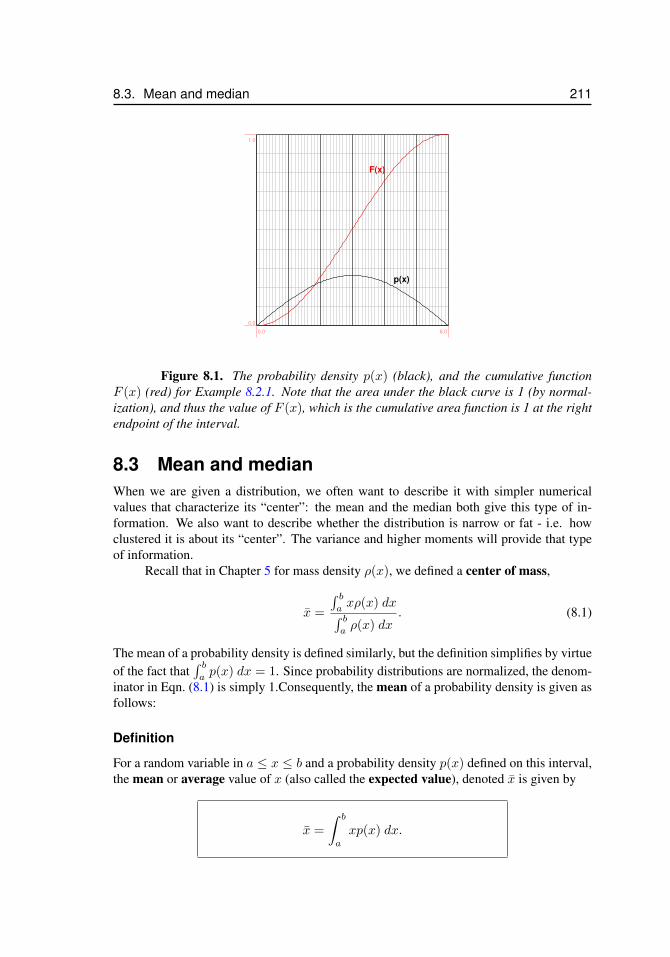
8.3. Mean and median 211
p(x)
F(x)
0.0 6.0
0.0
1.0
Figure 8.1. The probability density p(x) (black), and the cumulative functionF (x) (red) for Example 8.2.1. Note that the area under the black curve is 1 (by normal-ization), and thus the value of F (x), which is the cumulative area function is 1 at the rightendpoint of the interval.
8.3 Mean and medianWhen we are given a distribution, we often want to describe it with simpler numericalvalues that characterize its “center”: the mean and the median both give this type of in-formation. We also want to describe whether the distribution is narrow or fat - i.e. howclustered it is about its “center”. The variance and higher moments will provide that typeof information.
Recall that in Chapter 5 for mass density ρ(x), we defined a center of mass,
x =
∫ baxρ(x) dx∫ baρ(x) dx
. (8.1)
The mean of a probability density is defined similarly, but the definition simplifies by virtueof the fact that
∫ bap(x) dx = 1. Since probability distributions are normalized, the denom-
inator in Eqn. (8.1) is simply 1.Consequently, the mean of a probability density is given asfollows:
Definition
For a random variable in a ≤ x ≤ b and a probability density p(x) defined on this interval,the mean or average value of x (also called the expected value), denoted x is given by
x =
∫ b
a
xp(x) dx.
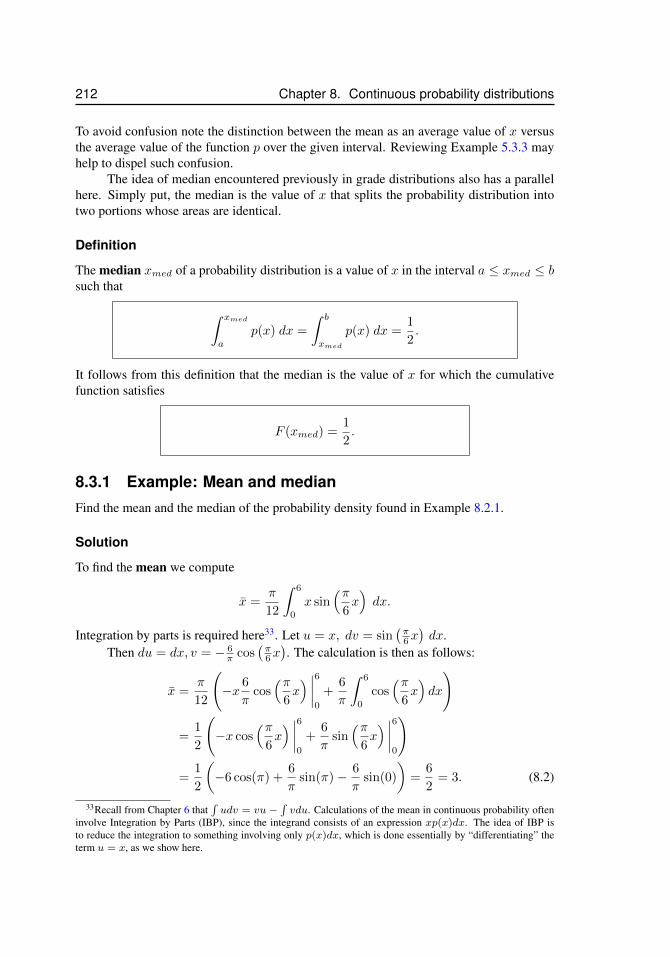
212 Chapter 8. Continuous probability distributions
To avoid confusion note the distinction between the mean as an average value of x versusthe average value of the function p over the given interval. Reviewing Example 5.3.3 mayhelp to dispel such confusion.
The idea of median encountered previously in grade distributions also has a parallelhere. Simply put, the median is the value of x that splits the probability distribution intotwo portions whose areas are identical.
Definition
The median xmed of a probability distribution is a value of x in the interval a ≤ xmed ≤ bsuch that
∫ xmed
a
p(x) dx =
∫ b
xmed
p(x) dx =1
2.
It follows from this definition that the median is the value of x for which the cumulativefunction satisfies
F (xmed) =1
2.
8.3.1 Example: Mean and medianFind the mean and the median of the probability density found in Example 8.2.1.
Solution
To find the mean we compute
x =π
12
∫ 6
0
x sin(π
6x)dx.
Integration by parts is required here33. Let u = x, dv = sin(π6x)dx.
Then du = dx, v = − 6π cos
(π6x). The calculation is then as follows:
x =π
12
(−x 6
πcos(π
6x) ∣∣∣∣6
0
+6
π
∫ 6
0
cos(π
6x)dx
)
=1
2
(−x cos
(π6x) ∣∣∣∣6
0
+6
πsin(π
6x) ∣∣∣∣6
0
)
=1
2
(−6 cos(π) +
6
πsin(π)− 6
πsin(0)
)=
6
2= 3. (8.2)
33Recall from Chapter 6 that∫udv = vu−
∫vdu. Calculations of the mean in continuous probability often
involve Integration by Parts (IBP), since the integrand consists of an expression xp(x)dx. The idea of IBP isto reduce the integration to something involving only p(x)dx, which is done essentially by “differentiating” theterm u = x, as we show here.
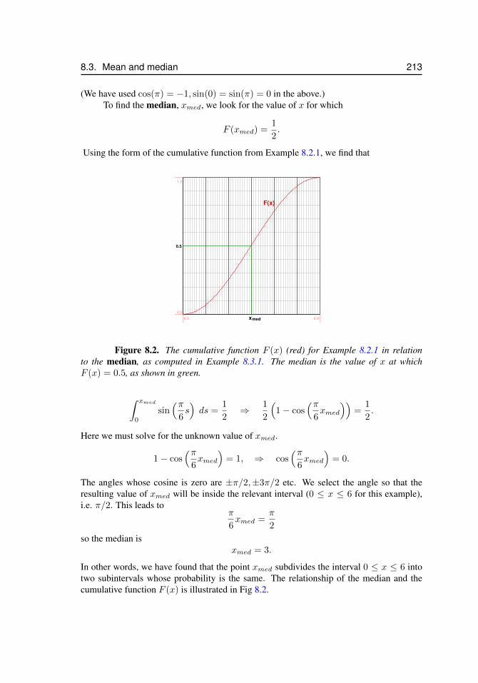
8.3. Mean and median 213
(We have used cos(π) = −1, sin(0) = sin(π) = 0 in the above.)To find the median, xmed, we look for the value of x for which
F (xmed) =1
2.
Using the form of the cumulative function from Example 8.2.1, we find that
F(x)
0.5
xmed0.0 6.0
0.0
1.0
Figure 8.2. The cumulative function F (x) (red) for Example 8.2.1 in relationto the median, as computed in Example 8.3.1. The median is the value of x at whichF (x) = 0.5, as shown in green.
∫ xmed
0
sin(π
6s)ds =
1
2⇒ 1
2
(1− cos
(π6xmed
))=
1
2.
Here we must solve for the unknown value of xmed.
1− cos(π
6xmed
)= 1, ⇒ cos
(π6xmed
)= 0.
The angles whose cosine is zero are ±π/2,±3π/2 etc. We select the angle so that theresulting value of xmed will be inside the relevant interval (0 ≤ x ≤ 6 for this example),i.e. π/2. This leads to
π
6xmed =
π
2
so the median isxmed = 3.
In other words, we have found that the point xmed subdivides the interval 0 ≤ x ≤ 6 intotwo subintervals whose probability is the same. The relationship of the median and thecumulative function F (x) is illustrated in Fig 8.2.
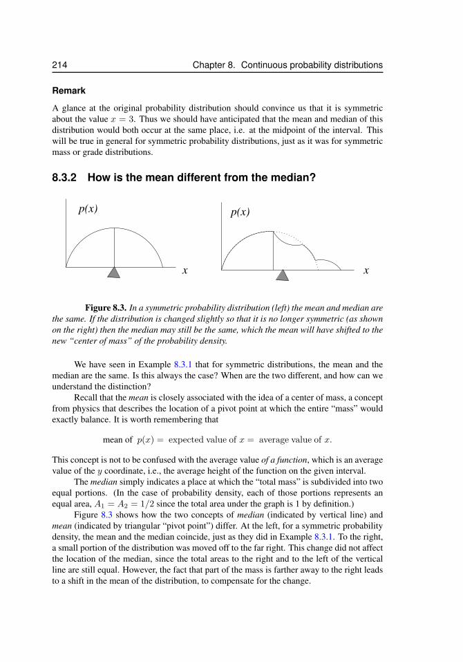
214 Chapter 8. Continuous probability distributions
Remark
A glance at the original probability distribution should convince us that it is symmetricabout the value x = 3. Thus we should have anticipated that the mean and median of thisdistribution would both occur at the same place, i.e. at the midpoint of the interval. Thiswill be true in general for symmetric probability distributions, just as it was for symmetricmass or grade distributions.
8.3.2 How is the mean different from the median?
p(x) p(x)
x x
Figure 8.3. In a symmetric probability distribution (left) the mean and median arethe same. If the distribution is changed slightly so that it is no longer symmetric (as shownon the right) then the median may still be the same, which the mean will have shifted to thenew “center of mass” of the probability density.
We have seen in Example 8.3.1 that for symmetric distributions, the mean and themedian are the same. Is this always the case? When are the two different, and how can weunderstand the distinction?
Recall that the mean is closely associated with the idea of a center of mass, a conceptfrom physics that describes the location of a pivot point at which the entire “mass” wouldexactly balance. It is worth remembering that
mean of p(x) = expected value of x = average value of x.
This concept is not to be confused with the average value of a function, which is an averagevalue of the y coordinate, i.e., the average height of the function on the given interval.
The median simply indicates a place at which the “total mass” is subdivided into twoequal portions. (In the case of probability density, each of those portions represents anequal area, A1 = A2 = 1/2 since the total area under the graph is 1 by definition.)
Figure 8.3 shows how the two concepts of median (indicated by vertical line) andmean (indicated by triangular “pivot point”) differ. At the left, for a symmetric probabilitydensity, the mean and the median coincide, just as they did in Example 8.3.1. To the right,a small portion of the distribution was moved off to the far right. This change did not affectthe location of the median, since the total areas to the right and to the left of the verticalline are still equal. However, the fact that part of the mass is farther away to the right leadsto a shift in the mean of the distribution, to compensate for the change.
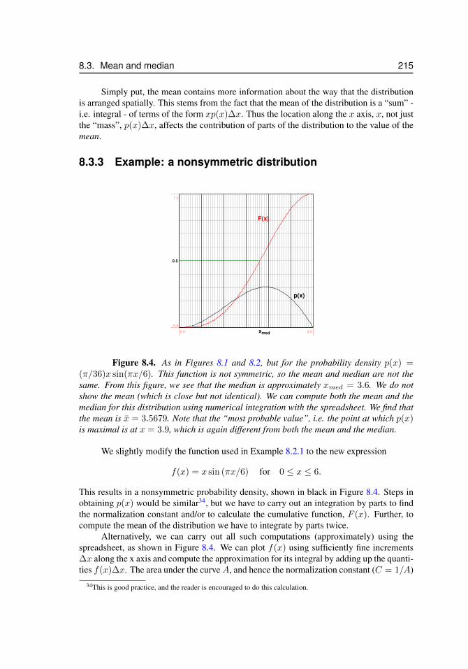
8.3. Mean and median 215
Simply put, the mean contains more information about the way that the distributionis arranged spatially. This stems from the fact that the mean of the distribution is a “sum” -i.e. integral - of terms of the form xp(x)∆x. Thus the location along the x axis, x, not justthe “mass”, p(x)∆x, affects the contribution of parts of the distribution to the value of themean.
8.3.3 Example: a nonsymmetric distribution
F(x)
0.5
xmed
p(x)
0.0 6.0
0.0
1.0
Figure 8.4. As in Figures 8.1 and 8.2, but for the probability density p(x) =(π/36)x sin(πx/6). This function is not symmetric, so the mean and median are not thesame. From this figure, we see that the median is approximately xmed = 3.6. We do notshow the mean (which is close but not identical). We can compute both the mean and themedian for this distribution using numerical integration with the spreadsheet. We find thatthe mean is x = 3.5679. Note that the “most probable value”, i.e. the point at which p(x)is maximal is at x = 3.9, which is again different from both the mean and the median.
We slightly modify the function used in Example 8.2.1 to the new expression
f(x) = x sin (πx/6) for 0 ≤ x ≤ 6.
This results in a nonsymmetric probability density, shown in black in Figure 8.4. Steps inobtaining p(x) would be similar34, but we have to carry out an integration by parts to findthe normalization constant and/or to calculate the cumulative function, F (x). Further, tocompute the mean of the distribution we have to integrate by parts twice.
Alternatively, we can carry out all such computations (approximately) using thespreadsheet, as shown in Figure 8.4. We can plot f(x) using sufficiently fine increments∆x along the x axis and compute the approximation for its integral by adding up the quanti-ties f(x)∆x. The area under the curveA, and hence the normalization constant (C = 1/A)
34This is good practice, and the reader is encouraged to do this calculation.
216 Chapter 8. Continuous probability distributions
will be thereby determined (at the point corresponding to the end of the interval, x = 6).It is then an easy matter to replot the revised function f(x)/A, which corresponds to thenormalized probability density. This is the curve shown in black in Figure 8.4. In the prob-lem sets, we leave as an exercise for the reader how to determine the median and the meanusing the same spreadsheet tool for a related (simpler) example.
8.4 Applications of continuous probabilityIn the next few sections, we explore applications of the ideas developed in this chapterto a variety of problems. We treat the decay of radioactive atoms, consider distribution ofheights in a population, and explore how the distribution of radii is related to the distributionof volumes in raindrop drop sizes. The interpretation of the probability density and thecumulative function, as well as the means and medians in these cases will form the mainfocus of our discussion.
8.4.1 Radioactive decayRadioactive decay is a probabilistic phenomenon: an atom spontaneously emits a particleand changes into a new form. We cannot predict exactly when a given atom will undergothis event, but we can study a large collection of atoms and draw some interesting conclu-sions.
We can define a probability density function that represents the probability per unittime that an atom would decay at time t. It turns out that a good candidate for such afunction is
p(t) = Ce−kt,
where k is a constant that represents the rate of decay (in units of 1/time) of the specificradioactive material. In principle, this function is defined over the interval 0 ≤ t ≤ ∞;that is, it is possible that we would have to wait a “very long time” to have all of the atomsdecay. This means that these integrals have to be evaluated “at infinity”, leading to animproper integral. Using this probability density for atom decay, we can characterize themean and median decay time for the material.
Normalization
We first find the constant of normalization, i.e. find the constant C such that∫ ∞0
p(t) dt =
∫ ∞0
Ce−kt dt = 1.
Recall that an integral of this sort, in which one of the endpoints is at infinity is called animproper integral35. Some care is needed in understanding how to handle such integrals,and in particular when they “exist” (in the sense of producing a finite value, despite the
35We have already encountered such integrals in Sections 3.8.5 and 7.3. See also, Chapter 7 for a more detaileddiscussion of improper integrals.
8.4. Applications of continuous probability 217
infinitely long domain of integration). We will delay full discussion to Chapter 7, and statehere the definition:
I =
∫ ∞0
Ce−kt dt ≡ limT→∞
IT where IT =
∫ T
0
Ce−kt dt.
The idea is to compute an integral over a finite interval 0 ≤ t ≤ T and then take a limit asthe upper endpoint, T goes to infinity (T →∞). We compute:
IT = C
∫ T
0
e−kt dt = C
[e−kt
−k
] ∣∣∣∣T0
=1
kC(1− e−kT ).
Now we take the limit:
I = limT→∞
IT = limT→∞
1
kC(1− e−kT ) =
1
kC(1− lim
T→∞e−kT ). (8.3)
To compute this limit, recall that for k > 0, T > 0, the exponential term in Eqn. 8.3 decaysto zero as T increases, so that
limT→∞
e−kT = 0.
Thus, the second term in braces in the integral I in Eqn. 8.3 will vanish as T →∞ so thatthe value of the improper integral will be
I = limT→∞
IT =1
kC.
To find the constant of normalization C we require that I = 1, i.e.1
kC = 1, which means
thatC = k.
Thus the (normalized) probability density for the decay is
p(t) = ke−kt.
This means that the fraction of atoms that decay between time t1 and t2 is
k
∫ t2
t1
e−kt dt.
Cumulative decays
The fraction of the atoms that decay between time 0 and time t (i.e. “any time up to timet” or “by time t - note subtle wording”36) is
F (t) =
∫ t
0
p(s) ds = k
∫ t
0
e−ks ds.
36Note that the precise English wording is subtle, but very important here. “By time t” means that the eventcould have happened at any time right up to time t.
218 Chapter 8. Continuous probability distributions
We can simplify this expression by integrating:
F (t) = k
[e−ks
−k
] ∣∣∣∣t0
= −[e−kt − e0
]= 1− e−kt.
Thus, the probability of the atoms decaying by time t (which means anytime up to time t)is
F (t) = 1− e−kt.
We note that F (0) = 0 and F (∞) = 1, as expected for the cumulative function.
Median decay time
As before, to determine the median decay time, tm (the time at which half of the atomshave decayed), we set F (tm) = 1/2. Then
1
2= F (tm) = 1− e−ktm ,
so we get
e−ktm =1
2, ⇒ ektm = 2, ⇒ ktm = ln 2, ⇒ tm =
ln 2
k.
Thus half of the atoms have decayed by this time. (Remark: this is easily recognized as thehalf life of the radioactive process from previous familiarity with exponentially decayingfunctions.)
Mean decay time
The mean time of decay t is given by
t =
∫ ∞0
tp(t) dt.
We compute this integral again as an improper integral by taking a limit as the top endpointincreases to infinity, i.e. we first find
IT =
∫ T
0
tp(t) dt,
and then sett = lim
T→∞IT .
To compute IT we use integration by parts:
IT =
∫ T
0
tke−kt dt = k
∫ T
0
te−kt dt.

8.4. Applications of continuous probability 219
Let u = t, dv = e−kt dt. Then du = dt, v = e−kt/(−k), so that
IT = k
[te−kt
(−k)−∫
e−kt
(−k)dt
] ∣∣∣∣T0
=
[−te−kt +
∫e−kt dt
] ∣∣∣∣T0
=
[−te−kt − e−kt
k
] ∣∣∣∣T0
=
[−Te−kT − e−kT
k+
1
k
]Now as T →∞, we have e−kT → 0 so that
t = limT→∞
IT =1
k.
Thus the mean or expected decay time is
t =1
k.
8.4.2 Discrete versus continuous probabilityIn Chapter 5.3, we compared the treatment of two types of mass distributions. We firstexplored a set of discrete masses strung along a “thin wire”. Later, we considered a single“bar” with a continuous distribution of density along its length. In the first case, there wasan unambiguous meaning to the concept of “mass at a point”. In the second case, we couldassign a mass to some section of the bar between, say x = a and x = b. (To do so we hadto integrate the mass density on the interval a ≤ x ≤ b.) In the first case, we talked aboutthe mass of the objects, whereas in the latter case, we were interested in the idea of density(mass per unit distance: Note that the units of mass density are not the same as the units ofmass.)
As we have seen so far in this chapter, the same dichotomy exists in the topic ofprobability. The example below provides some further insight to the connection betweencontinuous and discrete probability. In particular, we will see that one can arrive at theidea of probability density by refining a set of measurements and making the appropriatescaling. We explore this connection in more detail below.
8.4.3 Example: Student heightsSuppose we measure the heights of all UBC students. This would produce about 30,000data values37. We could make a graph and show how these heights are distributed. Forexample, we could subdivide the student body into those students between 0 and 1.5m, andthose between 1.5 and 3 meters. Our bar graph would contain two bars, with the numberof students in each height category represented by the heights of the bars, as shown inFigure 8.5(a).
Suppose we want to record this distribution in more detail. We could divide thepopulation into smaller groups by shrinking the size of the interval or “bin” into whichheight is subdivided. (An example is shown in Figure 8.5(b)). Here, by a “bin” we mean a
37I am grateful to David Austin for developing this example.
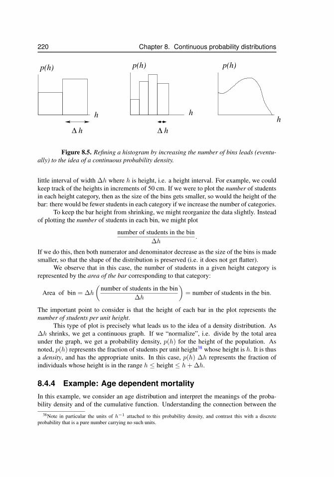
220 Chapter 8. Continuous probability distributions
h
p(h)
∆ h
h
p(h) p(h)
h
∆ h
Figure 8.5. Refining a histogram by increasing the number of bins leads (eventu-ally) to the idea of a continuous probability density.
little interval of width ∆h where h is height, i.e. a height interval. For example, we couldkeep track of the heights in increments of 50 cm. If we were to plot the number of studentsin each height category, then as the size of the bins gets smaller, so would the height of thebar: there would be fewer students in each category if we increase the number of categories.
To keep the bar height from shrinking, we might reorganize the data slightly. Insteadof plotting the number of students in each bin, we might plot
number of students in the bin∆h
.
If we do this, then both numerator and denominator decrease as the size of the bins is madesmaller, so that the shape of the distribution is preserved (i.e. it does not get flatter).
We observe that in this case, the number of students in a given height category isrepresented by the area of the bar corresponding to that category:
Area of bin = ∆h
(number of students in the bin
∆h
)= number of students in the bin.
The important point to consider is that the height of each bar in the plot represents thenumber of students per unit height.
This type of plot is precisely what leads us to the idea of a density distribution. As∆h shrinks, we get a continuous graph. If we “normalize”, i.e. divide by the total areaunder the graph, we get a probability density, p(h) for the height of the population. Asnoted, p(h) represents the fraction of students per unit height38 whose height is h. It is thusa density, and has the appropriate units. In this case, p(h) ∆h represents the fraction ofindividuals whose height is in the range h ≤ height ≤ h+ ∆h.
8.4.4 Example: Age dependent mortalityIn this example, we consider an age distribution and interpret the meanings of the proba-bility density and of the cumulative function. Understanding the connection between the
38Note in particular the units of h−1 attached to this probability density, and contrast this with a discreteprobability that is a pure number carrying no such units.
8.4. Applications of continuous probability 221
verbal description and the symbols we use to represent these concepts requires practice andexperience. Related problems are presented in the homework.
Let p(a) be a probability density for the probability of mortality of a female Canadiannon-smoker at age a, where 0 ≤ a ≤ 120. (We have chosen an upper endpoint of age120 since practically no Canadian female lives past this age at present.) Let F (a) be thecumulative distribution corresponding to this probability density. We would like to answerthe following questions:
(a) What is the probability of dying by age a?
(b) What is the probability of surviving to age a?
(c) Suppose that we are told that F (75) = 0.8 and that F (80) differs from F (75) by 0.11.Interpret this information in plain English. What is the probability of surviving to age80? Which is larger, F (75) or F (80)?
(d) Use the information in part (c) to estimate the probability of dying between the ages of75 and 80 years old. Further, estimate p(80) from this information.
Solution
(a) The probability of dying by age a is the same as the probability of dying any timeup to age a. Restated, this is the probability that the age of death is in the interval0 ≤ age of death ≤ a. The appropriate quantity is the cumulative function, for thisprobability density
F (a) =
∫ a
0
p(x) dx.
Remark: note that, as customary, x is playing the role of a “dummy variable”. We areintegrating over all ages between 0 and a, so we do not want to confuse the notationfor variable of integration, x and endpoint of the interval a. Hence the symbol x ratherthan a inside the integral.
(b) The probability of surviving to age a is the same as the probability of not dying beforeage a. By the elementary properties of probability discussed in the previous chapter,this is
1− F (a).
(c) F (75) = 0.8 means that the probability of dying some time up to age 75 is 0.8. (Thisalso means that the probability of surviving past this age would be 1-0.8=0.2.) Fromthe properties of probability, we know that the cumulative distribution is an increasingfunction, and thus it must be true that F (80) > F (75). Then F (80) = F (75)+0.11 =0.8 + 0.11 = 0.91. Thus the probability of surviving to age 80 is 1-0.91=0.09. Thismeans that 9% of the population will make it to their 80’th birthday.
(d) The probability of dying between the ages of 75 and 80 years old is exactly∫ 80
75
p(x) dx.
222 Chapter 8. Continuous probability distributions
However, we can also state this in terms of the cumulative function, since∫ 80
75
p(x) dx =
∫ 80
0
p(x) dx−∫ 75
0
p(x) dx = F (80)− F (75) = 0.11
Thus the probability of death between the ages of 75 and 80 is 0.11.
To estimate p(80), we use the connection between the probability density and the cu-mulative distribution39:
p(x) = F ′(x). (8.4)
Then it is approximately true that
p(x) ≈ F (x+ ∆x)− F (x)
∆x. (8.5)
(Recall the definition of the derivative, and note that we are approximating the deriva-tive by the slope of a secant line.) Here we have information at ages 75 and 80, so∆x = 80− 75 = 5, and the approximation is rather crude, leading to
p(80) ≈ F (80)− F (75)
5=
0.11
5= 0.022 per year.
Several important points merit attention in the above example. First, informationcontained in the cumulative function is useful. Differences in values of F between x = aand x = b are, after all, equivalent to an integral of the function
∫ bap(x)dx, and are the
probability of a result in the given interval, a ≤ x ≤ b. Second, p(x) is the derivative ofF (x). In the expression (8.5), we approximated that derivative by a small finite difference.Here we see at play many of the themes that have appeared in studying calculus: the con-nection between derivatives and integrals, the Fundamental Theorem of Calculus, and therelationship between tangent and secant lines.
8.4.5 Example: Raindrop size distributionIn this example, we find a rather non-intuitive result, linking the distribution of raindropsof various radii with the distribution of their volumes. This reinforces the caution neededin interpreting and handling probabilities.
During a Vancouver rainstorm, the distribution of raindrop radii is uniform for radii0 ≤ r ≤ 4 (where r is measured in mm) and zero for larger r. By a uniform distributionwe mean a function that has a constant value in the given interval. Thus, we are saying thatthe distribution looks like f(r) = C for 0 ≤ r ≤ 4.
(a) Determine what is the probability density for raindrop radii, p(r)? Interpret the mean-ing of that function.
39In Eqn. (8.4) there is no longer confusion between a variable of integration and an endpoint, so we couldrevert to the notation p(a) = F ′(a), helping us to identify the independent variable as age. However, we haveavoided doing so simply so that the formula in Eqn. (8.5) would be very recognizable as an approximation for aderivative.
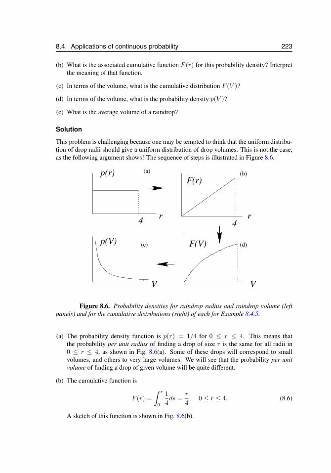
8.4. Applications of continuous probability 223
(b) What is the associated cumulative function F (r) for this probability density? Interpretthe meaning of that function.
(c) In terms of the volume, what is the cumulative distribution F (V )?
(d) In terms of the volume, what is the probability density p(V )?
(e) What is the average volume of a raindrop?
Solution
This problem is challenging because one may be tempted to think that the uniform distribu-tion of drop radii should give a uniform distribution of drop volumes. This is not the case,as the following argument shows! The sequence of steps is illustrated in Figure 8.6.
V
F(r)p(r)
F(V)
r r
V
4 4
(a) (b)
(c) (d)p(V)
Figure 8.6. Probability densities for raindrop radius and raindrop volume (leftpanels) and for the cumulative distributions (right) of each for Example 8.4.5.
(a) The probability density function is p(r) = 1/4 for 0 ≤ r ≤ 4. This means thatthe probability per unit radius of finding a drop of size r is the same for all radii in0 ≤ r ≤ 4, as shown in Fig. 8.6(a). Some of these drops will correspond to smallvolumes, and others to very large volumes. We will see that the probability per unitvolume of finding a drop of given volume will be quite different.
(b) The cumulative function is
F (r) =
∫ r
0
1
4ds =
r
4, 0 ≤ r ≤ 4. (8.6)
A sketch of this function is shown in Fig. 8.6(b).
224 Chapter 8. Continuous probability distributions
(c) The cumulative function F (r) is proportional to the radius of the drop. We use theconnection between radii and volume of spheres to rewrite that function in terms of thevolume of the drop: Since
V =4
3πr3 (8.7)
we have
r =
(3
4π
)1/3
V 1/3.
Substituting this expression into the formula (8.6), we get
F (V ) =1
4
(3
4π
)1/3
V 1/3.
We find the range of values of V by substituting r = 0, 4 into Eqn. (8.7) to getV = 0, 4
3π43. Therefore the interval is 0 ≤ V ≤ 43π43 or 0 ≤ V ≤ (256/3)π. The
function F (V ) is sketched in panel (d) of Fig. 8.6.
(d) We now use the connection between the probability density and the cumulative distri-bution, namely that p is the derivative of F . Now that the variable has been convertedto volume, that derivative is a little more “interesting”:
p(V ) = F ′(V )
Therefore,
p(V ) =1
4
(3
4π
)1/31
3V −2/3.
Thus the probability per unit volume of finding a drop of volume V in 0 ≤ V ≤ 43π43 is
not at all uniform. This probability density is shown in Fig. 8.6(c) This results from thefact that the differential quantity dr behaves very differently from dV , and reinforcesthe fact that we are dealing with density, not with a probability per se. We note thatthis distribution has smaller values at larger values of V .
(e) The range of values of V is
0 ≤ V ≤ 256π
3,
and therefore the mean volume is
V =
∫ 256π/3
0
V p(V )dV =1
12
(3
4π
)1/3 ∫ 256π/3
0
V · V −2/3dV
=1
12
(3
4π
)1/3 ∫ 256π/3
0
V 1/3dV =1
12
(3
4π
)1/33
4V 4/3
∣∣∣∣256π/3
0
=1
16
(3
4π
)1/3(256π
3
)4/3
=64π
3≈ 67mm3.
8.5. Moments of a probability density 225
8.5 Moments of a probability densityWe are now familiar with some of the properties of probability distributions. On this pagewe will introduce a set of numbers that describe various properties of such distributions.Some of these have already been encountered in our previous discussion, but now we willsee that these fit into a pattern of quantities called moments of the distribution.
8.5.1 Definition of momentsLet f(x) be any function which is defined and positive on an interval [a, b]. We might referto the function as a distribution, whether or not we consider it to be a probability density.Then we will define the following moments of this function:
zero’th moment M0 =
∫ b
a
f(x) dx
first moment M1 =
∫ b
a
x f(x) dx
second moment M2 =
∫ b
a
x2 f(x) dx
...
n’th moment Mn =
∫ b
a
xn f(x) dx.
Observe that moments of any order are defined by integrating the distribution f(x)with a suitable power of x over the interval [a, b]. However, in practice we will see thatusually moments up to the second are usefully employed to describe common attributes ofa distribution.
8.5.2 Relationship of moments to mean and variance of aprobability density
In the particular case that the distribution is a probability density, p(x), defined on theinterval a ≤ x ≤ b, we have already established the following :
M0 =
∫ b
a
p(x) dx = 1.
(This follows from the basic property of a probability density.) Thus The zero’th momentof any probability density is 1. Further
M1 =
∫ b
a
x p(x) dx = x = µ.
226 Chapter 8. Continuous probability distributions
That is, The first moment of a probability density is the same as the mean (i.e. expectedvalue) of that probability density. So far, we have used the symbol x to represent the meanor average value of x but often the symbol µ is also used to denote the mean.
The second moment, of a probability density also has a useful interpretation. Fromabove definitions, the second moment of p(x) over the interval a ≤ x ≤ b is
M2 =
∫ b
a
x2 p(x) dx.
We will shortly see that the second moment helps describe the way that density is dis-tributed about the mean. For this purpose, we must describe the notion of variance orstandard deviation.
Variance and standard deviation
Two children of approximately the same size can balance on a teeter-totter by sitting veryclose to the point at which the beam pivots. They can also achieve a balance by sitting at thevery ends of the beam, equally far away. In both cases, the center of mass of the distributionis at the same place: precisely at the pivot point. However, the mass is distributed verydifferently in these two cases. In the first case, the mass is clustered close to the center,whereas in the second, it is distributed further away. We may want to be able to describethis distinction, and we could do so by considering higher moments of the mass distribution.
Similarly, if we want to describe how a probability density distribution is distributedabout its mean, we consider moments higher than the first. We use the idea of the varianceto describe whether the distribution is clustered close to its mean, or spread out over a greatdistance from the mean.
Variance
The variance is defined as the average value of the quantity (distance from mean)2,where the average is taken over the whole distribution. (The reason for the square is thatwe would not like values to the left and right of the mean to cancel out.) For discreteprobability with mean, µ we define variance by
V =∑
(xi − µ)2pi.
For a continuous probability density, with mean µ, we define the variance by
V =
∫ b
a
(x− µ)2 p(x) dx.
The standard deviation
The standard deviation is defined as
8.5. Moments of a probability density 227
σ =√V .
Let us see what this implies about the connection between the variance and the momentsof the distribution.
Relationship of variance to second moment
From the equation for variance we calculate that
V =
∫ b
a
(x− µ)2 p(x) dx =
∫ b
a
(x2 − 2µx+ µ2) p(x) dx.
Expanding the integral leads to:
V =
∫ b
a
x2 p(x)dx−∫ b
a
2µx p(x) dx+
∫ b
a
µ2 p(x) dx
=
∫ b
a
x2 p(x)dx− 2µ
∫ b
a
x p(x) dx+ µ2
∫ b
a
p(x) dx.
We recognize the integrals in the above expression, since they are simply moments of theprobability distribution. Using the definitions, we arrive at
V = M2 − 2µ µ+ µ2.
Thus
V = M2 − µ2.
Observe that the variance is related to the second moment, M2 and to the mean, µ of thedistribution.
Relationship of variance to second moment
Using the above definitions, the standard deviation, σ can be expressed as
σ =√V =
√M2 − µ2.
8.5.3 Example: computing momentsConsider a probability density such that p(x) = C is constant for values of x in the interval[a, b] and zero for values outside this interval40. The area under the graph of this function
40As noted before, this is a uniform distribution. It has the shape of a rectangular band of height C and base(b− a).
228 Chapter 8. Continuous probability distributions
for a ≤ x ≤ b is A = C · (b − a) ≡ 1 (enforced by the usual property of a probabilitydensity), so it is easy to see that the value of the constant C should be C = 1/(b−a). Thus
p(x) =1
b− a, a ≤ x ≤ b.
We compute some of the moments of this probability density
M0 =
∫ b
a
p(x)dx =1
b− a
∫ b
a
1 dx = 1.
(This was already known, since we have determined that the zeroth moment of any proba-bility density is 1.) We also find that
M1 =
∫ b
a
x p(x) dx =1
b− a
∫ b
a
x dx =1
b− ax2
2
∣∣∣∣ba
=b2 − a2
2(b− a).
This last expression can be simplified by factoring, leading to
µ = M1 =(b− a)(b+ a)
2(b− a)=b+ a
2.
The value (b+a)/2 is a midpoint of the interval [a, b]. Thus we have found that the mean µis in the center of the interval, as expected for a symmetric distribution. The median wouldbe at the same place by a simple symmetry argument: half the area is to the left and halfthe area is to the right of this point.
To find the variance we calculate the second moment,
M2 =
∫ b
a
x2 p(x) dx =1
b− a
∫ b
a
x2 dx =
(1
b− a
)x3
3
∣∣∣∣ba
=b3 − a3
3(b− a).
Factoring simplifies this to
M2 =(b− a)(b2 + ab+ a2)
3(b− a)=b2 + ab+ a2
3.
The variance is then
V = M2 − µ2 =b2 + ab+ a2
3− (b+ a)2
4=b2 − 2ab+ a2
12=
(b− a)2
12.
The standard deviation is
σ =(b− a)
2√
3.

8.6. Summary 229
8.6 SummaryIn this chapter, we learned that the continuous probability density is a function specifyingthe probability per unit value (of the variable of interest), so that∫ b
a
p(x)dx = probability that x takes a value in the interval (a, b).
We also defined and studied the cumulative function
F (x) =
∫ x
a
p(s)ds = probability of a value in the interval (a, x).
We noted that by the Fundamental Theorem of Calculus, F (x) is an antiderivative of p(x)(or synonymously, p′(x) = F (x).)
The mean and median are two descriptors for some features of probability densities.For p(x) defined on an interval a ≤ x ≤ b and zero outside, the mean, (x, or sometimescalled µ) is
x =
∫ b
a
xp(x)dx
whereas the median, xmed is the value for which
F (xmed) =1
2.
Both mean and median correspond to the “center” of a symmetric distribution. If the dis-tribution is non-symmetric, a long tail in one direction will shift the mean toward thatdirection more strongly than the median. The variance of a probability density is
V =
∫ b
a
(x− µ)2 p(x) dx,
and the standard deviation isσ =√V .
This quantity describes the “width” of the distribution, i.e. how spread out (large σ) orclumped (small σ) it is.
We defined the n’th moment of a probability density as
Mn =
∫ b
a
xnp(x)dx,
and showed that the first few moments are related to mean and variance of the probability.Most of these concepts are directly linked to the analogous ideas in discrete probability,but in this chapter, we used integration in place of summation, to deal with the continuous,rather than the discrete case.
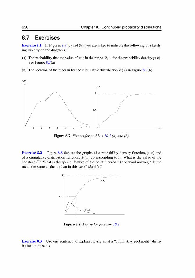
230 Chapter 8. Continuous probability distributions
8.7 ExercisesExercise 8.1 In Figures 8.7 (a) and (b), you are asked to indicate the following by sketch-ing directly on the diagrams.
(a) The probability that the value of x is in the range [2, 4] for the probability density p(x).See Figure 8.7(a)
(b) The location of the median for the cumulative distribution F (x) in Figure 8.7(b)
X
P(X)
1 2 3 4 5 6 7
1
F(X)
1/2
X
Figure 8.7. Figures for problem 10.1 (a) and (b).
Exercise 8.2 Figure 8.8 depicts the graphs of a probability density function, p(x) andof a cumulative distribution function, F (x) corresponding to it. What is the value of theconstant K? What is the special feature of the point marked * (one word answer)? Is themean the same as the median in this case? (Justify!)
P(X)
F(X)
K
K/2
*
Figure 8.8. Figure for problem 10.2
Exercise 8.3 Use one sentence to explain clearly what a “cumulative probability distri-bution” represents.
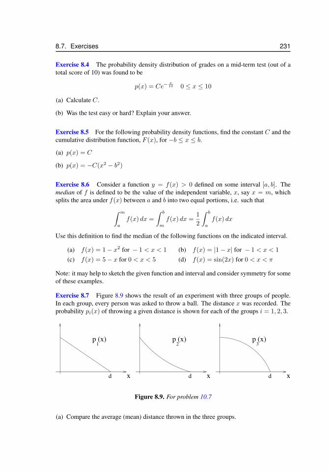
8.7. Exercises 231
Exercise 8.4 The probability density distribution of grades on a mid-term test (out of atotal score of 10) was found to be
p(x) = Ce−x10 0 ≤ x ≤ 10
(a) Calculate C.
(b) Was the test easy or hard? Explain your answer.
Exercise 8.5 For the following probability density functions, find the constant C and thecumulative distribution function, F (x), for −b ≤ x ≤ b.
(a) p(x) = C
(b) p(x) = −C(x2 − b2)
Exercise 8.6 Consider a function y = f(x) > 0 defined on some interval [a, b]. Themedian of f is defined to be the value of the independent variable, x, say x = m, whichsplits the area under f(x) between a and b into two equal portions, i.e. such that∫ m
a
f(x) dx =
∫ b
m
f(x) dx =1
2
∫ b
a
f(x) dx
Use this definition to find the median of the following functions on the indicated interval.
(a) f(x) = 1− x2 for − 1 < x < 1 (b) f(x) = |1− x| for − 1 < x < 1
(c) f(x) = 5− x for 0 < x < 5 (d) f(x) = sin(2x) for 0 < x < π
Note: it may help to sketch the given function and interval and consider symmetry for someof these examples.
Exercise 8.7 Figure 8.9 shows the result of an experiment with three groups of people.In each group, every person was asked to throw a ball. The distance x was recorded. Theprobability pi(x) of throwing a given distance is shown for each of the groups i = 1, 2, 3.
xd
p (x)1
xd
2p (x)
xd
p (x)3
Figure 8.9. For problem 10.7
(a) Compare the average (mean) distance thrown in the three groups.

232 Chapter 8. Continuous probability distributions
(b) Compare the median distances thrown in the three cases.
Exercise 8.8 Shown below is the probability density function which describes how muchof the Earth’s surface is at a given elevation (negative elevation means below sea level).
Figure 8.10. For problem 10.8
(a) Is more of the Earth’s surface above or below sea level? Use the concept of “median”to explain.
(b) Estimate what fraction of the Earth’s surface is below sea level.
Exercise 8.9 Suppose p(x) is the probability that a student in Math 103 gets a grade x.The median of p(x) is that value of x for which a typical student is equally likely to scoreabove as below.
(a) Suppose the range of scores is a ≤ x ≤ b and denote the median by m. Explain why∫ m
a
p(x) dx =
∫ b
m
p(x) dx =1
2
(b) Suppose that the students’ marks are described by the constant probability density func-tion p(x) = 1
100 on the interval 0 ≤ x ≤ 100. Find the average mark and the medianmark. What is the chance that a typical student scores better than the average mark?better than the median? Was the course easy or hard for these students?
(c) Now suppose that the students’ marks are described by p(x) = Cx on the interval0 ≤ x ≤ 100. What is the constant C? Find the average mark and the median. Whatis the chance that a typical student scores better than the average mark? better than themedian? In this case was the course “easier” or “harder” than in part (b). Explain why.
Exercise 8.10 Suppose F (x) is the cumulative distribution function for the height, x, ofNorth American adult males (in cm), and suppose p(x) is the probability density.
(a) What is the meaning of F (200) = 0.9?
(b) Interpret∫ 160
150p(x) dx = 0.2.
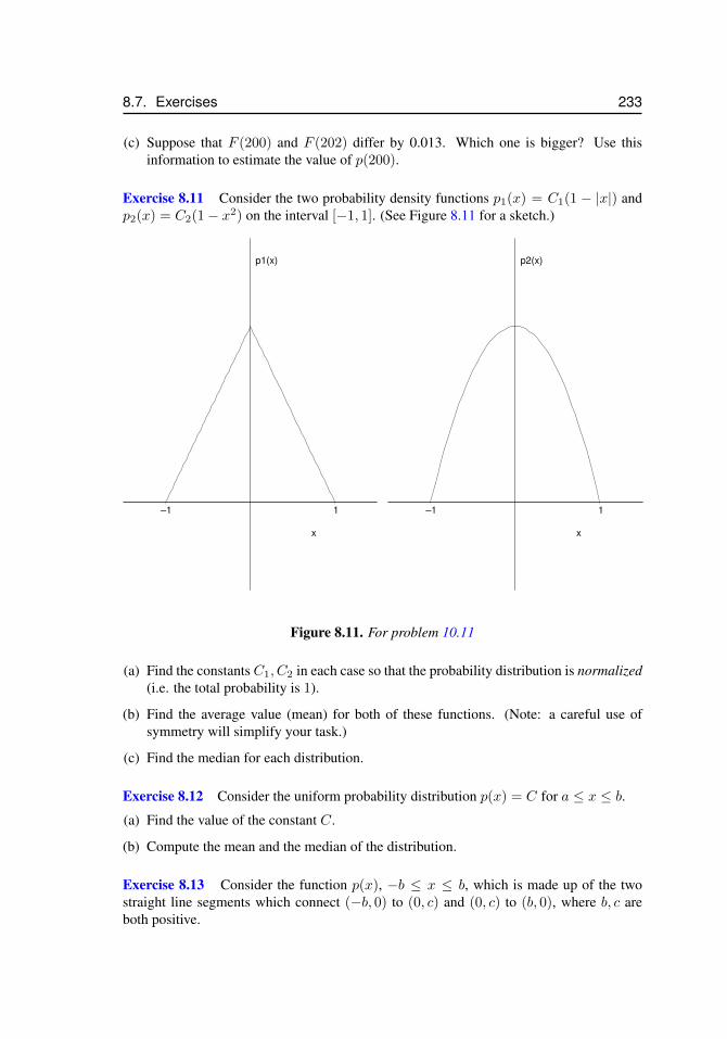
8.7. Exercises 233
(c) Suppose that F (200) and F (202) differ by 0.013. Which one is bigger? Use thisinformation to estimate the value of p(200).
Exercise 8.11 Consider the two probability density functions p1(x) = C1(1 − |x|) andp2(x) = C2(1− x2) on the interval [−1, 1]. (See Figure 8.11 for a sketch.)
p1(x)
–1 1
x
p2(x)
–1 1
x
Figure 8.11. For problem 10.11
(a) Find the constants C1, C2 in each case so that the probability distribution is normalized(i.e. the total probability is 1).
(b) Find the average value (mean) for both of these functions. (Note: a careful use ofsymmetry will simplify your task.)
(c) Find the median for each distribution.
Exercise 8.12 Consider the uniform probability distribution p(x) = C for a ≤ x ≤ b.(a) Find the value of the constant C.
(b) Compute the mean and the median of the distribution.
Exercise 8.13 Consider the function p(x), −b ≤ x ≤ b, which is made up of the twostraight line segments which connect (−b, 0) to (0, c) and (0, c) to (b, 0), where b, c areboth positive.
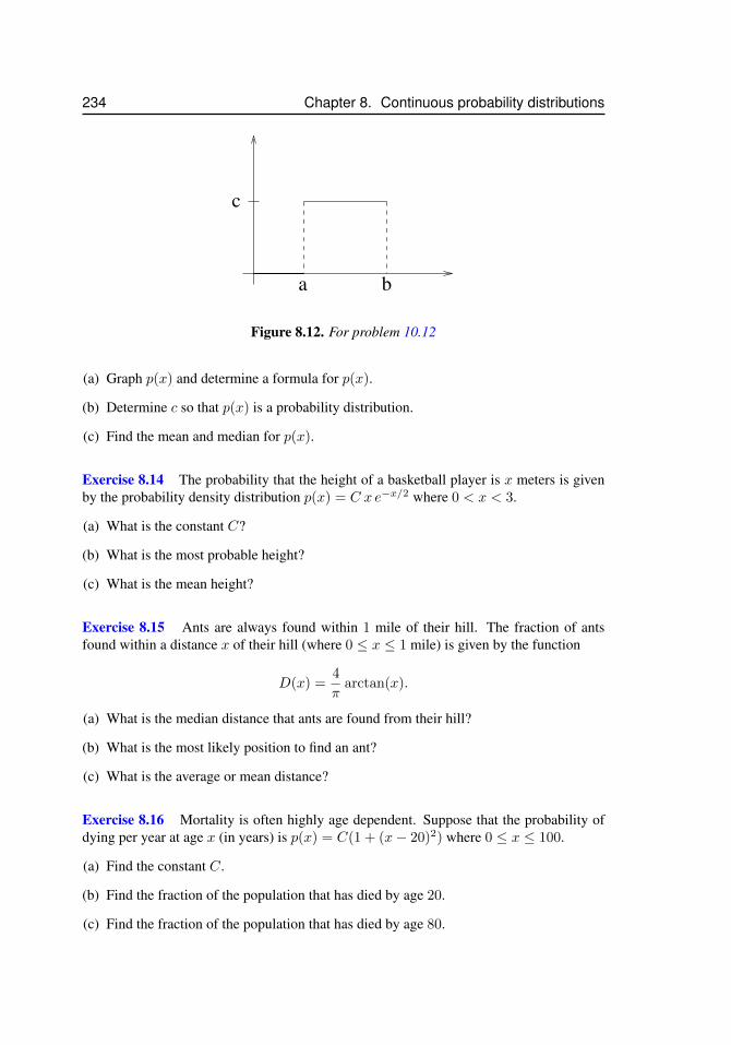
234 Chapter 8. Continuous probability distributions
a b
c
Figure 8.12. For problem 10.12
(a) Graph p(x) and determine a formula for p(x).
(b) Determine c so that p(x) is a probability distribution.
(c) Find the mean and median for p(x).
Exercise 8.14 The probability that the height of a basketball player is x meters is givenby the probability density distribution p(x) = C x e−x/2 where 0 < x < 3.
(a) What is the constant C?
(b) What is the most probable height?
(c) What is the mean height?
Exercise 8.15 Ants are always found within 1 mile of their hill. The fraction of antsfound within a distance x of their hill (where 0 ≤ x ≤ 1 mile) is given by the function
D(x) =4
πarctan(x).
(a) What is the median distance that ants are found from their hill?
(b) What is the most likely position to find an ant?
(c) What is the average or mean distance?
Exercise 8.16 Mortality is often highly age dependent. Suppose that the probability ofdying per year at age x (in years) is p(x) = C(1 + (x− 20)2) where 0 ≤ x ≤ 100.
(a) Find the constant C.
(b) Find the fraction of the population that has died by age 20.
(c) Find the fraction of the population that has died by age 80.
8.7. Exercises 235
(d) What is the mean lifetime in this population?
Exercise 8.17 Nonsymmetric distribution Consider the function
f(x) = cos(π
6x)
for 0 ≤ x ≤ 3.
This function is asymmetric on the given interval.
(a) Find the corresponding (normalized) probability density.
(b) Find the most probable value of x.
(c) Compute the mean and the median.
(d) Use a spreadsheet to determine the mean for this distribution by numerical integration.
(e) Use the spreadsheet to plot p(x) and the corresponding cumulative function F (x) onthe same graph. Using F (x), determine the value of the median.
Exercise 8.18 Suppose that x is a variable that takes on random non-negative values only.
(a) Show that the function below is a probability density distribution.
f(x) =2
(1 + x)3, 0 ≤ x <∞.
Note: the value of x here is not bounded, so you will have to compute an integral whoselimits are from 0 to infinity. Recall that this is called an improper integral. To computeits value, integrate from 0 to b and then consider b→∞.
(b) Find the probability that x takes on values in the interval [1, 4]
Exercise 8.19 The probability density function of a light bulb failing at time t, 0 ≤ t <∞, is given by p(t) = Ce−(0.1)t, where t is in days.
(a) Determine the constant C so that p(t) is a probability density function. In other wordsdetermine C so that
∫∞0C e−t/10 dt = 1 holds. This problem requires calculating an
improper integral.
(b) Find the function that describes the fraction of light bulbs failing by time t.
(c) What fraction of light bulbs are working after 20 days?
(d) Determine the mean and median times of failure.
Exercise 8.20 According to L. Glass and M. Mackey, the authors of a recent book Fromclocks to chaos, the rhythms of life p. 44: “The probability that a cell drawn at random froma large population has divided at time t ≥ 20 (minutes) is p(t) = Re−R(t−20), t ≥ 20,where R > 0 is some constant”. (They assume that cells never divide before time t = 20min.)
236 Chapter 8. Continuous probability distributions
(a) Find the mean time for division.
(b) What fraction of the cells have not divided by time t = 40 min?
Exercise 8.21 Given the probability distribution p(x) = C 1(1+x)2 , defined on 0 ≤ x <
∞.
(a) Find the probability that x takes on values in the interval [1, 4]. (You will first have tofind the value of the constant, C).
(b) Find the cumulative distribution function, F (x), for this probability density. Note thatthis problem involves calculating improper integrals.
(c) Sketch both p(x) and F (x),
Exercise 8.22 The probability that seeds will be dispersed a distance x (meters) awayfrom a parent tree is found to be p(x) = C e−x/10.
(a) Determine the value of the constant C so that p(x) is a probability density function.
(b) Determine the mean and median distances of dispersal.
(c) What is the variance V in the dispersal distance?
(d) Seeds that fall right under the tree (for x < 1 meter) fail to thrive because of com-petition with the parent tree and shading that stunts the growth of the seedling. Whatfraction of the seeds will fail to thrive? (Assume a 1-dimensional arrangement.) Notethat this problem involves calculating improper integrals.
Exercise 8.23 Survival Cells in a tissue culture are treated with an experimental medicine.Let t be the survival time of the cells in hours after receiving the treatment. The probabilitydensity function which describes this situation is p(t) = C e−Ct where 0 ≤ t ≤ ∞. If acell as a 70% chance of surviving two or more hours, find the value of the constant C.
Exercise 8.24 A mixture of cubic crystals of various sizes is made in the laboratory, andtheir sizes are measured. The probability density function, p(x), for the size of a crystal, x,(in millimeters), shown in Figure 8.13, is constant for 1 ≤ x ≤ 4.
(a) Write down the functional form of the probability density p(x) for crystal size and thecorresponding cumulative distribution F (x).
(b) Using the fact that the volume of a cube is V = x3, express this cumulative distributionin terms of the volume, i.e. find F in terms of V . (We’ll call this F (V )).
(c) Using what you have found for F (V ), determine the corresponding probability densityfunction p(V ) for crystal volume. (Hint: what is the connection between F (V ) andp(V )?)
(d) Use your result in (c) to calculate the mean volume, V , of the crystals.
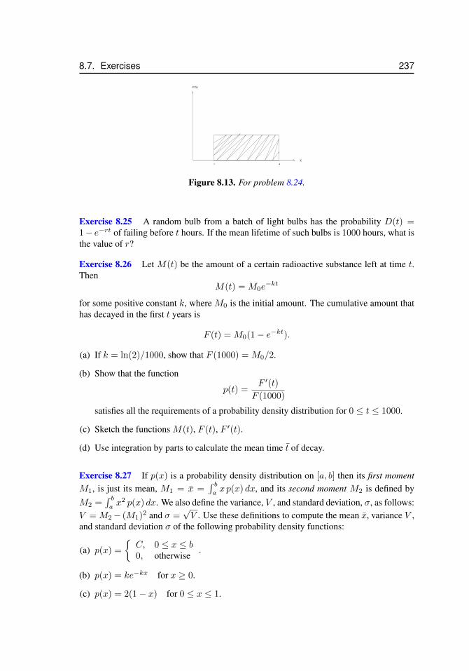
8.7. Exercises 237
X
P(X)
1 4
Figure 8.13. For problem 8.24.
Exercise 8.25 A random bulb from a batch of light bulbs has the probability D(t) =1− e−rt of failing before t hours. If the mean lifetime of such bulbs is 1000 hours, what isthe value of r?
Exercise 8.26 Let M(t) be the amount of a certain radioactive substance left at time t.Then
M(t) = M0e−kt
for some positive constant k, where M0 is the initial amount. The cumulative amount thathas decayed in the first t years is
F (t) = M0(1− e−kt).
(a) If k = ln(2)/1000, show that F (1000) = M0/2.
(b) Show that the function
p(t) =F ′(t)
F (1000)
satisfies all the requirements of a probability density distribution for 0 ≤ t ≤ 1000.
(c) Sketch the functions M(t), F (t), F ′(t).
(d) Use integration by parts to calculate the mean time t of decay.
Exercise 8.27 If p(x) is a probability density distribution on [a, b] then its first momentM1, is just its mean, M1 = x =
∫ bax p(x) dx, and its second moment M2 is defined by
M2 =∫ bax2 p(x) dx. We also define the variance, V , and standard deviation, σ, as follows:
V = M2− (M1)2 and σ =√V . Use these definitions to compute the mean x, variance V ,
and standard deviation σ of the following probability density functions:
(a) p(x) =
{C, 0 ≤ x ≤ b0, otherwise .
(b) p(x) = ke−kx for x ≥ 0.
(c) p(x) = 2(1− x) for 0 ≤ x ≤ 1.
238 Chapter 8. Continuous probability distributions
Exercise 8.28 Consider the uniform probability distribution p(x) = C for a ≤ x ≤ b.
(a) Find the variance and the standard deviation.
(b) Find the cumulative distribution function, F (x) for this probability density.
Exercise 8.29 Consider the function p(x) for −b ≤ x ≤ b, which is given by
p(x) =
c
bx+ c if − b ≤ x ≤ 0
−cbx+ c if 0 < x ≤ b
Find the variance V and the standard deviation σ of p(x).
Exercise 8.30 The function
p(x) = C sin(π
6x), 0 ≤ x ≤ 6,
is the probability density function for a random jump of x units at some large track meeting.
(a) Determine the constant C.
(b) Find the zeroth, the first, and the second moments of this probability distribution, i.e.calculate
I0 =
∫ 6
0
p(x) dx, I1 =
∫ 6
0
x p(x) dx, I2 =
∫ 6
0
x2 p(x) dx.
(c) Use the results of (b) to determine the mean, the variance, and the standard deviationof the jump distance.
Exercise 8.31 Consider the Normal (or Gaussian) distribution function given by
f(x) = Ce−x2
2 , −∞ < x <∞,
and suppose you are told (since it is not easy to calculate) that∫ ∞−∞
e−x2
2 dx =√
2π
(a) What value of the constant C should be used to make this function represent a proba-bility density distribution? This is called the Standard Normal distribution.
(b) Show that the mean and median are both 0.
(c) Show that the variance and the standard deviation are both 1. Note that this probleminvolves calculating improper integrals.
8.7. Exercises 239
Exercise 8.32 Consider the probability density distribution
p(x) =1√2πσ
e−(x−µ)2
2σ2 , −∞ < x <∞.
(a) Show that p(x) is a probability density function. Hint: use the substitution z = (x −µ)/σ.
(b) Show that the mean and median are both µ and the standard deviation is σ.
(c) Show that the most probable value of x occurs at x = µ.
Exercise 8.33 Quantum mechanics tells us that we can never know with complete cer-tainty where a particle is at any particular time. Instead, it gives us a probability densitywhich describes the chances that a particle is at some position. Einstein, as well as manyothers, found this difficult to accept, hence his famous quote “God does not play dice withthe universe.” Nevertheless, quantum mechanics has proven to be a theory which is re-markably consistent with physical observations.
For instance, if we are interested in how far the electron in a hydrogen atom is awayfrom its nucleus, the probability density function is p(r) = 4r2e−2r for 0 ≤ r <∞, wherer is the distance measured in “Bohr radii”. (One Bohr radius is the distance 5.29 · 10−11
meters.)
(a) Verify that p(r) is a probability density function.
(b) Sketch the probability density function by determining p(0), p′(r) and limr→∞ p(r).
(c) Near which value of r is the electron most likely to be found?
(d) Find the mean distance.
(e) Find the cumulative distribution F (r).What is the probability that the electron is foundwithin 1 Bohr radius of the nucleus?

240 Chapter 8. Continuous probability distributions
Chapter 9
Differential Equations
9.1 IntroductionA differential equation is a relationship between some (unknown) function and one of itsderivatives. Examples of differential equations were encountered in an earlier calculuscourse in the context of population growth, temperature of a cooling object, and speed of amoving object subjected to friction. In Section 4.2.4, we reviewed an example of a differ-ential equation for velocity, (4.8), and discussed its solution, but here, we present a moresystematic approach to solving such equations using a technique called separation of vari-ables. In this chapter, we apply the tools of integration to finding solutions to differentialequations. The importance and wide applicability of this topic cannot be overstated.
In this course, since we are concerned only with functions that depend on a singlevariable, we discuss ordinary differential equations (ODE’s), whereas later, after a mul-tivariate calculus course where partial derivatives are introduced, a wider class, of partialdifferential equations (PDE’s) can be studied. Such equations are encountered in many ar-eas of science, and in any quantitative analysis of systems where rates of change are linkedto the state of the system. Most laws of physics are of this form; for example, applyingthe familiar Newton’s law, F = ma, links the position of a pendulum’s mass to its accel-eration (second derivative of position).41 Many biological processes are also described bydifferential equations. The rate of growth of a population dN/dt depends on the size ofthat population at the given time N(t).
Constructing the differential equation that adequately represents a system of interestis an art that takes some thought and experience. In this process, which we call “modeling”,many simplifications are made so that the essential properties of a given system are cap-tured, leaving out many complicating details. For example, friction might be neglected in“modeling” a perfect pendulum. The details of age distribution might be neglected in mod-eling a growing population. Now that we have techniques for integration, we can devise anew approach to computing solutions of differential equations.
Given a differential equation and a starting value, the goal is to make a prediction
41Newton’s law states that force is proportional to acceleration. For a pendulum, the force is due to gravity, andthe acceleration is a second derivative of the x or y coordinate of the bob on the pendulum.
241
242 Chapter 9. Differential Equations
about the future behaviour of the system. This is equivalent to identifying the function thatsatisfies the given differential equation and initial value(s). We refer to such a function asthe solution to the initial value problem (IVP). In differential calculus, our explorationof differential equations was limited to those whose solution could be guessed, or whosesolution was supplied in advance. We also explored some of the fascinating geometric andqualitative properties of such equations and their predictions.
Now that we have techniques of integration, we can find the analytic solution to avariety of simple first-order differential equations (i.e. those involving the first derivativeof the unknown function). We will describe the technique of separation of variables. Thistechnique works for examples that are simple enough that we can isolate the dependentvariable (e.g. y) on one side of the equation, and the independent variable (e.g. time t) onthe other side.
9.2 Unlimited population growthWe start with a simple example that was treated thoroughly in the differential calculussemester of this course. We consider a population with per capita birth and mortality ratesthat are constant, irrespective of age, disease, environmental changes, or other effects. Weask how a population in such ideal circumstances would change over time. We build upa simple model (i.e. a differential equation) to describe this ideal case, and then proceedto find its solution. Solving the differential equation is accomplished by a new techniqueintroduced here, namely separation of variables. This reduces the problem to integrationand algebraic manipulation, allowing us to compute the population size at any time t. Bygoing through this process, we essentially convert information about the rate of change andstarting level of the population to a detailed prediction of the population at later times.42
9.2.1 A simple model for population growthLet y(t) represent the size of a population at time t. We will assume that at time t = 0, thepopulation level is specified, i.e. y(0) = y0 is some given constant. We want to find thepopulation at later times, given information about birth and mortality rates, (both of whichare here assumed to be constant over time).
The population changes through births and mortality. Suppose that b > 0 is the percapita average birth rate, and m > 0 the per capita average mortality rate. The assumptionthat b, m are both constants is a simplification that neglects many biological effects, butwill be used for simplicity in this first example.
The statement that the population increases through births and decreases due to mor-tality, can be restated as
rate of change of y = rate of births− rate of mortality
where the rate of births is given by the product of the per capita average birth rate b and thepopulation size y. Similarly, the rate of mortality is given by my. Translating the rate of
42Of course, we must keep in mind that such predictions are based on simplifying assumptions, and are to betaken as an approximation of any real population growth.
9.2. Unlimited population growth 243
change into the corresponding derivative of y leads to
dy
dt= by −my = (b−m)y.
Let us define the new constant,k = b−m.
Then k is the net per capita growth rate of the population. We can distinguish two possiblecases: b > m means that there are more births then deaths, so we expect the populationto grow. b < m means that there are more deaths than births, so that the population willeventually go extinct. There is also a marginal case that b = m, for which k = 0, where thepopulation does not change at all. To summarize, this simple model of unlimited growthleads to the differential equation and initial condition:
dy
dt= ky, y(0) = y0. (9.1)
Recall that a differential equation together with an initial condition is called an initial valueproblem. To find a solution to such a problem, we look for the function y(t) that describesthe population size at any future time t, given its initial size at time t = 0.
9.2.2 Separation of variables and integrationWe here introduce the technique, separation of variables, that will be used in all theexamples described in this chapter. Since the differential equation (9.1) is relatively simple,this first example will be relatively straightforward. We would like to determine y(t) giventhe differential equation
dy
dt= ky.
Rather than integrating this equation as is43, we use an alternate approach, consid-ering dt and dy as “differentials” in the sense defined in Section 6.1. We rearrange andrewrite the above equation in the form
1
ydy = k dt, (9.2)
This step of putting expressions involving the independent variable t on one side and ex-pressions involving the dependent variable y on the opposite side gives rise to the name“separation of variables”.
Now, the LHS of Eqn. (9.2) depends only on the variable y, and the RHS only on t.The constant k will not interfere with any integration step. Moreover, integrating each sideof Eqn. (9.2) can be carried out independently.
To determine the appropriate intervals for integration, we observe that when timesweeps over some interval 0 ≤ t ≤ T (from initial to final time), the value of y(t) will
43We may be tempted to integrate both sides of this equation with respect to the independent variable t, e.g.writing
∫ dydtdt =
∫ky dt + C, (where C is some constant), but this is not very useful, since the integral on
the right hand side (RHS) can only be carried out if we know the function y = y(t), which we are trying todetermine.
244 Chapter 9. Differential Equations
change over a corresponding interval y0 ≤ y ≤ y(T ). Here y0 is the given starting valueof y (prescribed by the initial condition in (9.1)). We do not yet know y(T ), but our goalis to find that value, i.e to predict the future behaviour of y. Integrating leads to∫ y(T )
y0
1
ydy =
∫ T
0
k dt = k
∫ T
0
dt,
ln |y|∣∣∣∣y(T )
y0
= kt
∣∣∣∣T0
,
ln |y(T )| − ln |y(0)| = k(T − 0),
ln
∣∣∣∣y(T )
y0
∣∣∣∣ = kT,
y(T )
y0= ekT ,
y(T ) = y0ekT .
But this result holds for any arbitrary final time, T . In other words, since this is true for anytime we chose, we can set T = t, arriving at the desired solution
y(t) = y0ekt. (9.3)
The above formula relates the predicted value of y at any time t to its initial value, and toall the parameters of the problem. Observe that plugging in t = 0, we get y(0) = y0e
kt =y0e
0 = y0, so that the solution (9.3) satisfies the initial condition. We leave as an exercisefor the reader44 to validate that the function in(9.3) also satisfies the differential equation in(9.1).
By solving the initial value problem (9.1), we have determined that, under ideal con-ditions, when the net per capita growth rate t is constant, a population will grow expo-nentially with time. Recall that this validates results that we had encountered in our firstcalculus course.
9.3 Terminal velocity and steady statesHere we revisit the equation for velocity of a falling object that we first encountered in Sec-tion 4.2.4. We wish to derive the appropriate differential equation governing that velocity,and find the solution v(t) as a function of time. We will first reconsider the simplest case ofuniformly accelerated motion (i.e. where friction is neglected), as in Section 4.2.3. We theninclude friction, as in Section 4.2.4 and use the new technique of separation of variables toshortcut the method of solution.
44This kind of check is good practice and helps to spot errors. Simply differentiate Eqn. (9.3) and show that theresult is the same as k times the original function, as required by the equation (9.1).
9.3. Terminal velocity and steady states 245
9.3.1 Ignoring friction: the uniformly accelerated caseLet v(t) and a(t) be the velocity and the acceleration, respectively of an object fallingunder the force of gravity at time t. We take the positive direction to be downwards, forconvenience. Suppose that at time t = 0, the object starts from rest, i.e. the initial velocityof the object is known to be v(0) = 0. When friction is neglected, the object will accelerate,
a(t) = g,
which is equivalent to the statement that the velocity increases at a constant rate,
dv
dt= g. (9.4)
Because g is constant, we do not need to use separation of variables, i.e. we can integrateeach side of this equation directly45. Writing∫
dv
dtdt =
∫g dt+ C = g
∫dt+ C,
where C is an integration constant, we arrive at
v(t) = gt+ C. (9.5)
Here we have used (on the LHS) that v is the antiderivative of dv/dt. (equivalently, we cansimplify the integral
∫dvdt dt =
∫dv = v). Plugging in v(0) = 0 into Eqn. (9.5) leads to
0 = g · 0 + C = C, so the constant we need is C = 0 and the velocity satisfies
v(t) = gt.
We have just arrived at a result that parallels Eqn. (4.4) of Section 4.2.3 (in slightly differentnotation).
9.3.2 Including friction: the case of terminal velocityWhen a falling object experiences the force of friction, it cannot accelerate indefinitely. Infact, a frictional force retards the downwards motion. To a good approximation, that forceis proportional to the velocity.
A force balance for the falling object leads to
ma(t) = mg − γv(t),
where γ is the frictional coefficient. For an object of constant mass, we can divide throughby m, so
a(t) = g − γ
mv(t).
45It is important to note the distinction between this simple example and other cases where separation of vari-ables is required. It would not be wrong to use separation of variables to find the solution for Eqn. (9.4), but itwould just be “overkill”, since simple integration of the each side of the equation “as is” does the job.
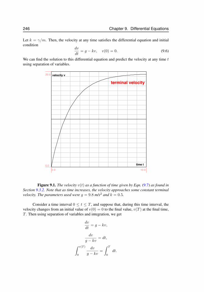
246 Chapter 9. Differential Equations
Let k = γ/m. Then, the velocity at any time satisfies the differential equation and initialcondition
dv
dt= g − kv, v(0) = 0. (9.6)
We can find the solution to this differential equation and predict the velocity at any time tusing separation of variables.
terminal velocity
time t
velocity v
0.0 10.00.0
20.0
Figure 9.1. The velocity v(t) as a function of time given by Eqn. (9.7) as found inSection 9.3.2. Note that as time increases, the velocity approaches some constant terminalvelocity. The parameters used were g = 9.8 m/s2 and k = 0.5.
Consider a time interval 0 ≤ t ≤ T , and suppose that, during this time interval, thevelocity changes from an initial value of v(0) = 0 to the final value, v(T ) at the final time,T . Then using separation of variables and integration, we get
dv
dt= g − kv,
dv
g − kv= dt,∫ v(T )
0
dv
g − kv=
∫ T
0
dt.
9.3. Terminal velocity and steady states 247
Substitute u = g − kv for the integral on the left hand side. Then du = −kdv, dv =(−1/k)du, so we get an integral of the form
−1
k
∫1
udu = −1
kln |u|.
After replacing u by g − kv, we arrive at
−1
kln |g − kv|
∣∣∣∣v(T )
0
= t
∣∣∣∣T0
.
We use the fact that v(0) = 0 to write this as
−1
k(ln |g − kv(T )| − ln |g|) = T,
−1
k
(ln
∣∣∣∣g − kv(T )
g
∣∣∣∣) = T,
ln
∣∣∣∣g − kv(T )
g
∣∣∣∣ = −kT.
We are finished with the integration step, but the function we are trying to find, v(T )is still tangled up inside an expression involving the natural logarithm. Extricating it willinvolve some subtle reasoning about signs because there is an absolute value to contendwith. As a first step, we exponentiate both sides to remove the logarithm.∣∣∣∣g − kv(T )
g
∣∣∣∣ = e−kT ⇒ |g − kv(T )| = ge−kT .
Because the constant g is positive, we could remove absolute values signs from it. Tosimplify further, we have to consider the sign of the term inside the absolute value in thenumerator. In the case we are considering here, v(0) = 0. This will mean that the quantityg− kv(T ) is always be non-negative (i.e. g− kv(T ) ≥ 0). We will verify this fact shortly.For the moment, supposing this is true, we can write
|g − kv(T )| = g − kv(T ) = ge−kT ,
and finally solve for v(T ) to obtain our final result,
v(T ) =g
k(1− e−kT ).
Here we note that v(T ) can never be larger than g/k since the term (1 − e−kT ) is always≤ 1. Hence, we were correct in assuming that g − kv(T ) ≥ 0.
As before, the above formula relating velocity to time holds for any choice of thefinal time T , so we can write, in general,
v(t) =g
k(1− e−kt). (9.7)
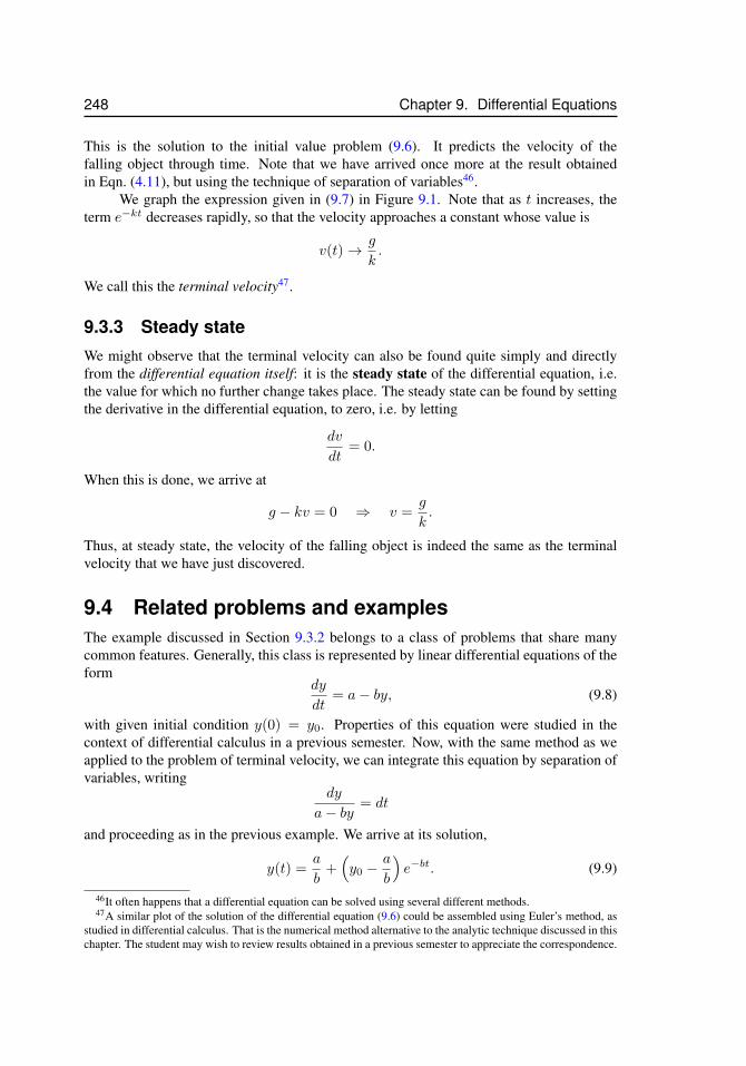
248 Chapter 9. Differential Equations
This is the solution to the initial value problem (9.6). It predicts the velocity of thefalling object through time. Note that we have arrived once more at the result obtainedin Eqn. (4.11), but using the technique of separation of variables46.
We graph the expression given in (9.7) in Figure 9.1. Note that as t increases, theterm e−kt decreases rapidly, so that the velocity approaches a constant whose value is
v(t)→ g
k.
We call this the terminal velocity47.
9.3.3 Steady stateWe might observe that the terminal velocity can also be found quite simply and directlyfrom the differential equation itself: it is the steady state of the differential equation, i.e.the value for which no further change takes place. The steady state can be found by settingthe derivative in the differential equation, to zero, i.e. by letting
dv
dt= 0.
When this is done, we arrive at
g − kv = 0 ⇒ v =g
k.
Thus, at steady state, the velocity of the falling object is indeed the same as the terminalvelocity that we have just discovered.
9.4 Related problems and examplesThe example discussed in Section 9.3.2 belongs to a class of problems that share manycommon features. Generally, this class is represented by linear differential equations of theform
dy
dt= a− by, (9.8)
with given initial condition y(0) = y0. Properties of this equation were studied in thecontext of differential calculus in a previous semester. Now, with the same method as weapplied to the problem of terminal velocity, we can integrate this equation by separation ofvariables, writing
dy
a− by= dt
and proceeding as in the previous example. We arrive at its solution,
y(t) =a
b+(y0 −
a
b
)e−bt. (9.9)
46It often happens that a differential equation can be solved using several different methods.47A similar plot of the solution of the differential equation (9.6) could be assembled using Euler’s method, as
studied in differential calculus. That is the numerical method alternative to the analytic technique discussed in thischapter. The student may wish to review results obtained in a previous semester to appreciate the correspondence.
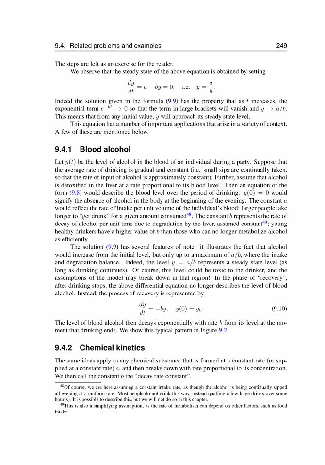
9.4. Related problems and examples 249
The steps are left as an exercise for the reader.We observe that the steady state of the above equation is obtained by setting
dy
dt= a− by = 0, i.e. y =
a
b.
Indeed the solution given in the formula (9.9) has the property that as t increases, theexponential term e−bt → 0 so that the term in large brackets will vanish and y → a/b.This means that from any initial value, y will approach its steady state level.
This equation has a number of important applications that arise in a variety of context.A few of these are mentioned below.
9.4.1 Blood alcoholLet y(t) be the level of alcohol in the blood of an individual during a party. Suppose thatthe average rate of drinking is gradual and constant (i.e. small sips are continually taken,so that the rate of input of alcohol is approximately constant). Further, assume that alcoholis detoxified in the liver at a rate proportional to its blood level. Then an equation of theform (9.8) would describe the blood level over the period of drinking. y(0) = 0 wouldsignify the absence of alcohol in the body at the beginning of the evening. The constant awould reflect the rate of intake per unit volume of the individual’s blood: larger people takelonger to “get drunk” for a given amount consumed48. The constant b represents the rate ofdecay of alcohol per unit time due to degradation by the liver, assumed constant49; younghealthy drinkers have a higher value of b than those who can no longer metabolize alcoholas efficiently.
The solution (9.9) has several features of note: it illustrates the fact that alcoholwould increase from the initial level, but only up to a maximum of a/b, where the intakeand degradation balance. Indeed, the level y = a/b represents a steady state level (aslong as drinking continues). Of course, this level could be toxic to the drinker, and theassumptions of the model may break down in that region! In the phase of “recovery”,after drinking stops, the above differential equation no longer describes the level of bloodalcohol. Instead, the process of recovery is represented by
dy
dt= −by, y(0) = y0. (9.10)
The level of blood alcohol then decays exponentially with rate b from its level at the mo-ment that drinking ends. We show this typical pattern in Figure 9.2.
9.4.2 Chemical kineticsThe same ideas apply to any chemical substance that is formed at a constant rate (or sup-plied at a constant rate) a, and then breaks down with rate proportional to its concentration.We then call the constant b the “decay rate constant”.
48Of course, we are here assuming a constant intake rate, as though the alcohol is being continually sippedall evening at a uniform rate. Most people do not drink this way, instead quaffing a few large drinks over somehour(s). It is possible to describe this, but we will not do so in this chapter.
49This is also a simplifying assumption, as the rate of metabolism can depend on other factors, such as foodintake.
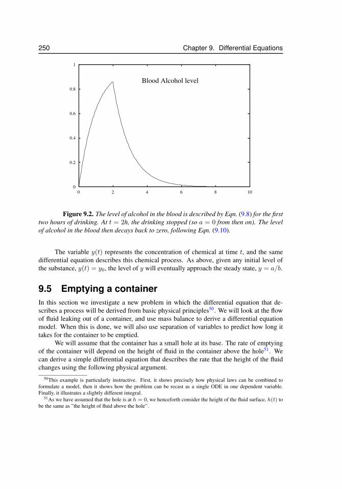
250 Chapter 9. Differential Equations
0
0.2
0.4
0.6
0.8
1
0 2 4 6 8 10
Blood Alcohol level
Figure 9.2. The level of alcohol in the blood is described by Eqn. (9.8) for the firsttwo hours of drinking. At t = 2h, the drinking stopped (so a = 0 from then on). The levelof alcohol in the blood then decays back to zero, following Eqn. (9.10).
The variable y(t) represents the concentration of chemical at time t, and the samedifferential equation describes this chemical process. As above, given any initial level ofthe substance, y(t) = y0, the level of y will eventually approach the steady state, y = a/b.
9.5 Emptying a containerIn this section we investigate a new problem in which the differential equation that de-scribes a process will be derived from basic physical principles50. We will look at the flowof fluid leaking out of a container, and use mass balance to derive a differential equationmodel. When this is done, we will also use separation of variables to predict how long ittakes for the container to be emptied.
We will assume that the container has a small hole at its base. The rate of emptyingof the container will depend on the height of fluid in the container above the hole51. Wecan derive a simple differential equation that describes the rate that the height of the fluidchanges using the following physical argument.
50This example is particularly instructive. First, it shows precisely how physical laws can be combined toformulate a model, then it shows how the problem can be recast as a single ODE in one dependent variable.Finally, it illustrates a slightly different integral.
51As we have assumed that the hole is at h = 0, we henceforth consider the height of the fluid surface, h(t) tobe the same as ”the height of fluid above the hole”.
9.5. Emptying a container 251
A
v t∆
aa
h
Figure 9.3. We investigate the time it takes to empty a container full of fluid byderiving a differential equation model and solving it using the methods developed in thischapter. A is the cross-sectional area of the cylindrical tank, a is the cross-sectional areaof the hole through which fluid drains, v(t) is the velocity of the fluid, and h(t) is the timedependent height of fluid remaining in the tank (indicated by the dashed line). The volumeof fluid leaking out in a time span ∆t is av∆t - see small cylindrical volume indicated onthe right.
9.5.1 Conservation of massSuppose that the container is a cylinder, with a constant cross sectional area A > 0, asshown in Fig. 9.3. Suppose that the area of the hole is a. The rate that fluid leaves throughthe hole must balance with the rate that fluid decreases in the container. This principle iscalled mass balance. We will here assume that the density of water is constant, so that wecan talk about the net changes in volume (rather than mass).
We refer to V (t) as the volume of fluid in the container at time t. Note that for thecylindrical container, V (t) = Ah(t) where A is the cross-sectional area and h(t) is theheight of the fluid at time t. The rate of change of V is
dV
dt= −(rate volume lost as fluid flows out).
(The minus sign indicates that the volume is decreasing).At every second, some amount of fluid leaves through the hole. Suppose we are
told that the velocity of the water molecules leaving the hole is precisely v(t) in units ofcm/sec. (We will find out how to determine this velocity shortly.) Then in one second,those particles have moved a distance v cm/sec · 1 sec = v cm. In fact, all the particles ina little cylinder of length v behind these molecules have also left the hole. Indeed, if weknow the area of the hole, we can determine precisely what volume of water exits throughthe hole each second, namely
rate volume lost as fluid flows out = va.
(The small inset in Fig. 9.3 shows a little “cylindrical unit” of fluid that flows out of thehole per second. The area is a and the length of that little volume is v. Thus the volumeleaving per second is va.)
252 Chapter 9. Differential Equations
So far we have a relationship between the volume of fluid in the tank and the velocityof the water exiting the hole:
dV
dt= −av.
Now we need to determine the velocity v of the flow to complete the formulation of theproblem.
9.5.2 Conservation of energyThe fluid “picks up speed” because it has “dropped” by a height h from the top of the fluidsurface to the hole. In doing so, a small mass of water has simply exchanged some potentialenergy (due to its relative height above the hole) for kinetic energy (expressed by how fastit is moving). Potential energy of a small mass of water (m) at height h will be mgh,whereas when the water flows out of the hole, its kinetic energy is given by (1/2)mv2
where v is velocity. Thus, for these to balance (so that total energy is conserved) we have
1
2mv2 = mgh.
(Here v = v(t) is the instantaneous velocity of the fluid leaving the hole and h = h(t) isthe height of the water column.) This allows us to relate the velocity of the fluid leavingthe hole to the height of the water in the tank, i.e.
v2 = 2gh ⇒ v =√
2gh. (9.11)
In fact, both the height of fluid and its exit velocity are constantly changing as the fluiddrains, so we might write [v(t)]2 = 2gh(t) or v(t) =
√2gh(t). We have arrived at this
result using an energy balance argument.
9.5.3 Putting it togetherWe now combine the various pieces of information to arrive at the model, a differentialequation for a single (unknown) function of time. There are three time-dependent variablesthat were discussed above, the volume V (t), the height h(t), of the velocity v(t). It provesconvenient to express everything in terms of the height of water in the tank, h(t), thoughthis choice is to some extent arbitrary. Keeping units in an equation consistent is essential.Checking for unit consistency can help to uncover errors in equations, including differentialequations.
Recall that the volume of the water in the tank, V (t) is related to the height of fluidh(t) by
V (t) = Ah(t),
whereA > 0 is a constant, the cross-sectional area of the tank. We can simplify as follows:
dV
dt=d(Ah(t))
dt= A
d(h(t))
dt.
But by previous steps and Eqn. (9.11)
dV
dt= −av = −a
√2gh.
9.5. Emptying a container 253
Thus
Ad(h(t))
dt= −a
√2gh,
or simply put,dh
dt= − a
A
√2gh = −k
√h. (9.12)
where k is a constant that depends on the size and shape of the cylinder and its hole:
k =a
A
√2g.
If the area of the hole is very small relative to the cross-sectional area of the tank, thenk will be very small, so that the tank will drain very slowly (i.e. the rate of change in hper unit time will not be large). On a planet with a very high gravitational force, the sametank will drain more quickly. A taller column of water drains faster. Once its height hasbeen reduced, its rate of draining also slows down. We comment that Equation (9.12) hasa minus sign, signifying that the height of the fluid decreases.
Using simple principles such as conservation of mass and conservation of energy,we have shown that the height h(t) of water in the tank at time t satisfies the differentialequation (9.12). Putting this together with the initial condition (height of fluid h0 at timet = 0), we arrive at initial value problem to solve:
dh
dt= −k
√h, h(0) = h0. (9.13)
Clearly, this equation is valid only for h non-negative. We also remark that Eqn. (9.13) isnonlinear52 as it involves the variable h in a nonlinear term,
√h. Next, we use separation
of variables to find the height as a function of time.
9.5.4 Solution by separation of variablesThe equation (9.13) shows how height of fluid is related to its rate of change, but we areinterested in an explicit formula for fluid height h versus time t. To obtain that relationship,we must determine the solution to this differential equation. We do this using separation ofvariables. (We will also use the initial condition h(0) = h0 that accompanies Eqn. (9.13).)As usual, rewrite the equation in the separated form,
dh√h
= −kdt,
We integrate from t = 0 to t = T , during which the height of fluid that started as h0
becomes some new height h(T ) to be determined.∫ h(T )
h0
1√hdh = −k
∫ T
0
dt.
52In many cases, nonlinear differential equations are more challenging than linear ones. However, exampleschosen in this chapter are simple enough that we will not experience the true challenges of such nonlinearities.
254 Chapter 9. Differential Equations
Now integrate both sides and simplify:
h1/2
(1/2)
∣∣∣∣h(T )
h0
= −kT
2(√
h(T )−√h0
)= −kT√
h(T ) = −kT2
+√h0
h(T ) =
(√h0 − k
T
2
)2
.
Since this is true for any time t, we can also write the form of the solution as
h(t) =
(√h0 − k
t
2
)2
. (9.14)
Eqn. (9.14) predicts fluid height remaining in the tank versus time t. In Fig. 9.4 we showsome of the “solution curves”53, i.e. functions of the form Eqn. (9.14) for a variety of initialfluid height values h0. We can also use our results to predict the emptying time, as shownin the next section.
9.5.5 How long will it take the tank to empty?The tank will be empty when the height of fluid is zero. Setting h(t) = 0 in Eqn. 9.14(√
h0 − kt
2
)2
= 0.
Solving this equation for the emptying time te, we get
kte2
=√h0 ⇒ te =
2√h0
k.
The time it takes to empty the tank depends on the initial height of water in the tank. Threeexamples are shown in Figure 9.4 for initial heights of h0 = 2.5, 5, 10. The emptying timedepends on the square-root of the initial height. This means, for instance, that doubling theheight of fluid initially in the tank only increases the time it takes by a factor of
√2 ≈ 1.41.
Making the hole smaller has a more direct “proportional” effect, since we have found thatk = (a/A)
√2g.
53As before, this figure was produced by plotting the analytic solution (9.14). A numerical method alternativewould use Euler’s Method and the spreadsheet to obtain the (approximate) solution directly from the initial valueproblem (9.13).
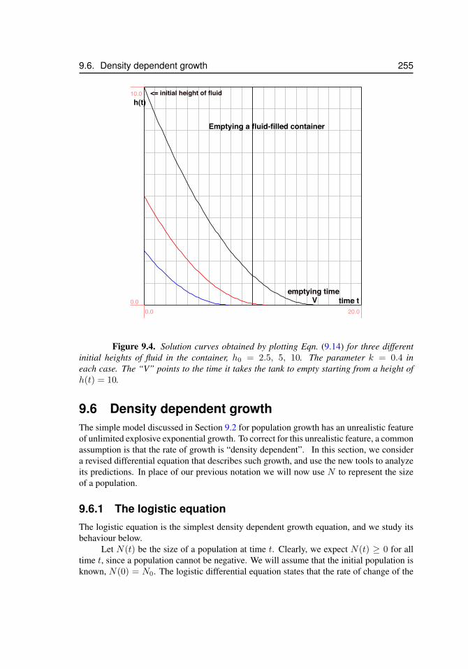
9.6. Density dependent growth 255
h(t)
time t
<= initial height of fluid
emptying timeV
Emptying a fluid-filled container
0.0 20.00.0
10.0
Figure 9.4. Solution curves obtained by plotting Eqn. (9.14) for three differentinitial heights of fluid in the container, h0 = 2.5, 5, 10. The parameter k = 0.4 ineach case. The “V” points to the time it takes the tank to empty starting from a height ofh(t) = 10.
9.6 Density dependent growthThe simple model discussed in Section 9.2 for population growth has an unrealistic featureof unlimited explosive exponential growth. To correct for this unrealistic feature, a commonassumption is that the rate of growth is “density dependent”. In this section, we considera revised differential equation that describes such growth, and use the new tools to analyzeits predictions. In place of our previous notation we will now use N to represent the sizeof a population.
9.6.1 The logistic equationThe logistic equation is the simplest density dependent growth equation, and we study itsbehaviour below.
Let N(t) be the size of a population at time t. Clearly, we expect N(t) ≥ 0 for alltime t, since a population cannot be negative. We will assume that the initial population isknown, N(0) = N0. The logistic differential equation states that the rate of change of the
256 Chapter 9. Differential Equations
population is given bydN
dt= rN
(K −NK
). (9.15)
Here r > 0 is called the intrinsic growth rate and K > 0 is called the carrying capacity.K reflects that size of the population that can be sustained by the given environment. Wecan understand this equation as a modified growth law in which the “density dependent”term, r(K −N)/K, replaces the previous constant net growth rate k.
9.6.2 Scaling the equationThe form of the equation can be simplified if we measure the population in units of thecarrying capacity, instead of “numbers of individuals”. i.e. if we define a new quantity
y(t) =N(t)
K.
This procedure is called scaling. To see this, consider dividing each side of the logisticequation (9.15) by the constant K. Then
1
K
dN
dt=
r
KN
(K −NK
).
We now group terms conveniently, forming
d(NK )
dt= r
(N
K
)(1−
(N
K
)).
Replacing (N/K) by y in each case, we obtain the scaled equation and initial conditiongiven by
dy
dt= ry(1− y), y(0) = y0. (9.16)
Now the variable y(t) measures population size in “units” of the carrying capacity, andy0 = N0/K is the scaled initial population level. Here again is an initial value problem,like Eqn. (9.13), but unlike Eqn. (9.1), the logistic differential equation is nonlinear. Thatis, the variable y appears in a nonlinear expression (in fact a quadratic) in the equation.
9.6.3 Separation of variablesHere we will solve Eqn. (9.16) by separation of variables. The idea is essentially the sameas our previous examples, but is somewhat more involved. To show an alternative methodof handling the integration, we will treat both sides as indefinite integrals. Separating thevariables leads to
1
y(1− y)dy = r dt∫
1
y(1− y)dy =
∫r dt+K.
9.6. Density dependent growth 257
The integral on the right will lead to rt + K where K is some constant of integration thatwe need to incorporate since we do not have endpoints on our integrals. But we must workharder to evaluate the integral on the left. We can do so by partial fractions, the techniquedescribed in Section 6.6. Details are given in Section 9.6.4.
9.6.4 Application of partial fractionsLet
I =
∫1
y(1− y)dy.
Then for some constants A,B we can write
I =
∫A
y+
B
1− ydy = A ln |y| −B ln |1− y|.
(The minus sign in front of B stems from the fact that letting u = 1 − y would lead todu = −dy.) We can find A,B from the fact that
A
y+
B
1− y=
1
y(1− y),
so thatA(1− y) +By = 1.
This must be true for all y, and in particular, substituting in y = 0 and y = 1 leads toA = 1, B = 1 so that
I = ln |y| − ln |1− y| = ln
∣∣∣∣ y
1− y
∣∣∣∣.9.6.5 The solution of the logistic equationWe now have to extract the quantity y from the equation
ln
∣∣∣∣ y
1− y
∣∣∣∣ = rt+ C0.
That is, we want y as a function of t. After exponentiating both sides we need to removethe absolute value. We will now assume that y is initially smaller than 1, and show that itremains so. In that case, everything inside the absolute value is positive, and we can write
y(t)
1− y(t)= ert+C0 = eC0ert = Cert.
In the above step, we have simply renamed the constant, eC0 by the new name C forsimplicity. C > 0 is now also an arbitrary constant whose value will be determined fromthe initial conditions. Indeed, if we substitute t = 0 into the most recent equation, we findthat
y(0)
1− y(0)= Ce0 = C,
258 Chapter 9. Differential Equations
so thatC =
y0
1− y0.
We will use this fact shortly. What remains now is some algebra to isolate the desiredfunction y(t)
y(t) = (1− y(t))Cert
y(t)(1 + Cert
)= Cert
y(t) =Cert
(1 + Cert)=
11C e−rt + 1
. (9.17)
The desired function is now expressed in terms of the time t, and the constants r, C. Wecan also express it in terms of the initial value of y, i.e. y0, by using what we know to betrue about the constant C, i.e. C = y0/(1− y0). When we do so, we arrive at
y(t) =1
1−y0y0
e−rt + 1=
y0
y0 + (1− y0)e−rt. (9.18)
Some typical solution curves of the logistic equation are shown in Fig. 9.5.
9.6.6 What this solution tells usWe have arrived at the function that describes the scaled population as a function of timeas predicted by the scaled logistic equation, (9.16). The level of population (in units of thecarrying capacity K) follows the time-dependent function
y(t) =y0
y0 + (1− y0)e−rt. (9.19)
We can convert this result to an equivalent expression for the unscaled total populationN(t)by recalling that y(t) = N(t)/K. Substituting this for y(t), and noting that y0 = N0/Kleads to
N(t) =N0
N0 + (K −N0)e−rtK. (9.20)
It is left as an exercise for the reader to check this claim.Check it! Now recall that r > 0. This means that e−rt is a decreasing function of time. There-
fore, (9.19) implies that, after a long time, the term e−rt in the denominator will be negli-gibly small, and so
y(t)→ y0
y0= 1,
so that y will approach the value 1. This means that
N
K→ 1 or simply N(t)→ K.
The population will thus settle into a constant level, i.e., a steady state, at which no furtherchange will occur.
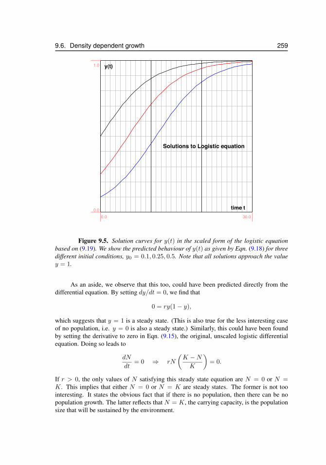
9.6. Density dependent growth 259
y(t)
time t
Solutions to Logistic equation
0.0 30.00.0
1.0
Figure 9.5. Solution curves for y(t) in the scaled form of the logistic equationbased on (9.19). We show the predicted behaviour of y(t) as given by Eqn. (9.18) for threedifferent initial conditions, y0 = 0.1, 0.25, 0.5. Note that all solutions approach the valuey = 1.
As an aside, we observe that this too, could have been predicted directly from thedifferential equation. By setting dy/dt = 0, we find that
0 = ry(1− y),
which suggests that y = 1 is a steady state. (This is also true for the less interesting caseof no population, i.e. y = 0 is also a steady state.) Similarly, this could have been foundby setting the derivative to zero in Eqn. (9.15), the original, unscaled logistic differentialequation. Doing so leads to
dN
dt= 0 ⇒ rN
(K −NK
)= 0.
If r > 0, the only values of N satisfying this steady state equation are N = 0 or N =K. This implies that either N = 0 or N = K are steady states. The former is not toointeresting. It states the obvious fact that if there is no population, then there can be nopopulation growth. The latter reflects that N = K, the carrying capacity, is the populationsize that will be sustained by the environment.

260 Chapter 9. Differential Equations
In summary, we have shown that the behaviour of the logistic equation for populationgrowth is more realistic than the simpler exponential growth we studied earlier. We sawin Figure 9.5, that a small population will grow, but only up to some constant level (thecarrying capacity). Integration, and in particular the use of partial fractions allowed us tomake a full prediction of the behaviour of the population level as a function of time, givenby Eqn. (9.20).
9.7 Extensions and other population models: the“Law of Mortality”
There are many variants of the logistic model that are used to investigate the growth ormortality of a population. Here we extend tools to another example, the gradual decline ofa group of individuals born at the same time. Such a group is called a “cohort”.54. In 1825,Gompertz suggested that the rate of mortality, m would depend on the age of the individu-als. Because we consider a group of people who were born at the same time, we can trade”age” for ”time”. Essentially, Gompertz assumed that mortality is not constant: it is lowat first, and increase as individuals age. Gompertz argued that mortality increases expo-nentially. This turns out to be equivalent to the assumption that the logarithm of mortalityincreases linearly with time.55 It is easy to see that these two statements are equivalent:Suppose we assume that for some constants A > 0, µ > 0,
ln(m(t)) = A+ µt. (9.21)
Then Eqn. (9.21) means that
t
ln( )m
A
slope µ
log mortality
age,
Figure 9.6. In the Gompertz Law of Mortality, it is assumed that the log of mor-tality increases linearly with time, as depicted by Eqn. 9.21 and by the solid curve in thisdiagram. Here the slope of ln(m) versus time (or age) is µ. For real populations, themortality looks more like the dashed curve.
54This section was formulated with help from Lu Fan55In actual fact, this is likely true for some range of ages. Infant mortality is generally higher than mortality
for young children, whereas mortality levels off or even decreases slightly for those oldest old who have survivedpast the average lifespan.
9.7. Extensions and other population models: the “Law of Mortality” 261
m(t) = eA+µt = eAeµt
SinceA is constant, so is eA. For simplicity we define Let us definem0 = eA. (m0 = m(0)is the so-called “birth mortality” i.e. value of m at age 0.) Thus, the time-dependentmortality is
m = m(t) = m0eµt. (9.22)
9.7.1 Aging and Survival curves for a cohort:We now study a population model having Gompertz mortality, together with the followingadditional assumptions.
1. All individuals are assumed to be identical.
2. There is “natural” mortality, but no other type of removal. This means we ignore themortality caused by epidemics, by violence and by wars.
3. We consider a single cohort, and assume that no new individuals are introduced (e.g.by immigration)56.
We will now study the size of a “cohort”, i.e. a group of people who were born in the sameyear. We will denote by N(t) the number of people in this group who are alive at time t,where t is time since birth, i.e. age. Let N(0) = N0 be the initial number of individuals inthe cohort.
9.7.2 Gompertz ModelAll the people in the cohort were born at time (age) t = 0, and there were N0 of them atthat time. That number changes with time due to mortality. Indeed,
The rate of change of cohort size = −[number of deaths per unit time]= −[mortality rate] · [cohort size]
Translating to mathematical notation, we arrive at the differential equation
dN(t)
dt= −m(t)N(t),
and using information about the size of the cohort at birth leads to the initial condition,N(0) = N0. Together, this leads to the initial value problem
dN(t)
dt= −m(t)N(t), N(0) = N0.
Note similarity to Eqn. (9.1), but now mortality is time-dependent.In the Problem set, we apply separation of variables and integrate over the time in-
terval [0, T ]: to show that the remaining population at age t is
N(t) = N0e−m0
µ (eµt−1).
56Note that new births would contribute to other cohorts.
262 Chapter 9. Differential Equations
9.8 SummaryIn this chapter, we used integration methods to find the analytical solutions to a variety ofdifferential equations where initial values were prescribed.
We investigated a number of population growth models:
1. Exponential growth, given by dydt = ky, with initial population level y(0) = y0
was investigated (Eqn. (9.1)). This model had an unrealistic feature that growth isunlimited.
2. The Logistic equation dNdt = rN
(K−NK
)was analyzed (Eqn. (9.15)), showing that
density-dependent growth can correct for the above unrealistic feature.
3. The Gompertz equation, dN(t)dt = −m(t)N(t), was solved to understand how age-
dependent mortality affects a cohort of individuals.
In each of these cases, we used separation of variables to “integrate” the differentialequation, and predict the population as a function of time.
We also investigated several other physical models in this chapter, including thevelocity of a falling object subject to drag force. This led us to study a differential equationof the form dy
dt = a − by. By slight reinterpretation of terms in this equation, we can useresults to understand chemical kinetics and blood alcohol levels, as well as a host of otherscientific applications.
Section 9.5, the “centerpiece” of this chapter, illustrated the detailed steps that go intothe formulation of a differential equation model for flow of liquid out of a container. Herewe saw how conservation statements and simplifying assumptions are interpreted together,to arrive at a differential equation model. Such ideas occur in many scientific problems, inchemistry, physics, and biology.
9.9. Excercises 263
9.9 ExcercisesExercise 9.1 Use separation of variables to solve the following differential equations withgiven initial conditions.
(a) dydt = −2t y, y(0) = 10
(b) dydt = y(1− y), y(0) = 0.5. (Hint: 1
y(y−1) = 1y−1 −
1y .)
Exercise 9.2 Consider the differential equation dydt = 1− y and initial condition y(0) =
0.5.
(a) Solve for y as a function of t using separation of variables.
(b) Use the initial condition to find the value of C.
Exercise 9.3 Consider the differential equation dydt = 1 + y2 and initial condition y(0) =
0.5.
(a) Solve for y as a function of t using separation of variables.
(b) Use the initial condition to find the value of C.
Exercise 9.4 Consider the differential equation dydt = 1− y2 and initial condition y(0) =
0.5. Solve using separation of variables (Hint: use partial fractions.)
Exercise 9.5 Solve the following differential equation dydt = ky2/3 and initial condition
y(0) = y0, assuming that k > 0 is a constant.
Exercise 9.6 A certain cylindrical water tank has a hole in the bottom, out of which waterflows. The height of water in the tank, h(t), can be described by the differential equationdhdt = −k
√h where k is a positive constant. If the height of the water is initially h0,
determine how much time elapses before the tank is empty.
Exercise 9.7 The position of a particle is described by
dx
dt=√
1− x2, 0 ≤ t ≤ π
2
(a) Find the position as a function of time given that the particle starts at x = 0 initially.
(b) Where is the particle when t = π/2?
(c) At which position(s) is the particle moving the fastest? The slowest?
Exercise 9.8 In an experiment involving yeast cells, it was determined that mortality ofthe cells increased at a linear rate, i.e. that at time t after the beginning of the experimentthe mortality rate was m(t) = m0 + r t. The experiment was started with N0 cells at timet = 0. Let N(t) represent the population size of the cells at time t.
264 Chapter 9. Differential Equations
(a) If no “birth” occurs, thendN(t)
dt= −m(t)N(t).
Solve this differential equation by separation of variables, i.e find N(t) as a functionof time.
(b) Suppose cells are “born” at a constant rate b, so that the differential equation is
dN(t)
dt= −m(t)N(t) + bN(t).
Determine how this affects the population size at time t.
Exercise 9.9 Muscle cells are known to be powered by filaments of the protein actinwhich slide past one another. The filaments are moved by cross-bridges of myosin, that actlike little motors, which attach, pull the filaments, and then detach. Let n be the fraction ofmyosin cross-bridges that are attached at time t. A model for cross-bridge attachment is:
dn
dt= k1(1− n)− k2n, n(0) = n0
where k1 > 0, k2 > 0 are constants.
(a) Solve this differential equation and determine the fraction of attached cross-bridgesn(t) as a function of time t.
(b) What value does n(t) approach after a long time?
(c) Suppose k1 = 1.0 and k2 = 0.2. Starting from n(0) = 0, how long does it take for50% of the cross-bridges to become attached ?
Exercise 9.10 The velocity of an object falling under the effect of gravity and air re-sistance is given by: dv
dt = f(v) = g − kv with v(0) = v0, where g > 0 denotes theacceleration due to gravity and k > 0 is a frictional coefficient (both constant).
(a) Sketch the function f(v) as a function of v. Identify a value of v = v∗ for which nochange occurs, i.e., for which f(v∗) = 0. This is called a steady state value of thevelocity or a fixed point. Interpret what this value represents.
(b) Explain what happens if the initial velocity is larger or smaller than this steady statevalue. Will the velocity increase or decrease? (Recall that the sign of the derivativedv/dt tells us whether v(t) is an increasing or decreasing function of t).
(c) Use separation of variables to find the function v(t).
Exercise 9.11 A model for the velocity of a sky diver (slightly different from the modelwe have already studied) is
dv
dt= 9− v2
9.9. Excercises 265
(a) What is this skydiver’s “terminal velocity”, v∞? That is, near what velocity will thesky diver eventually stabilize?
(b) Starting from rest, how long will it take to reach half of v∞?
Exercise 9.12 Newton’s Law of Cooling Consider the differential equation for Newton’sLaw of Cooling
dT
dt= −k(T − E)
for a constant k > 0, temperature of the environment E and the initial condition: T (0) =T0. Solve this differential equation by the method of separation of variables i.e. find T (t).Interpret your result.
Exercise 9.13 Let V (t) be the volume of a spherical cell that is expanding by absorbingwater from its surface area. Suppose that the rate of increase of volume is simply pro-portional to the surface area of the sphere, and that, initially, the volume is V0. Find adifferential equation that describes the way that V changes. Use the connection betweensurface area and volume in a sphere to rewrite your differential equation in terms of thevolume alone. You should get an equation in the form
dV
dt= kV 2/3,
where k is some constant. Solve the differential equation to show how the volume changesas a function of the time. (Hint: recall that for a sphere, V = (4/3)πr3, S = 4πr2.)
Exercise 9.14 According to Klaassen and Lindstrom (1996) J theor. Biol. 183:29-34, the“fuel load” (nectar) carried by a hummingbird, F (t) depends on the rate of intake (fromflowers) and the rate of consumption due to metabolism. They assume that intake takesplace at a constant rate α. They also assume that consumption increases when the bird isheavier (carrying more fuel). Suppose that fuel is consumed at a rate proportional to theamount of fuel being carried (with proportionality constant β).
(a) What features are being neglected or simplified in this model?
(b) Write down the differential equation model for F (t).
(c) Find F (t) as a function of time t.
(d) Klaassen and Lindstrom determined that for a hummingbird, α = 0.48 g fuel per dayand β = 0.09 per day. Determine the steady state level of fuel carried by the bird.(Note: use the fact that at steady state, the rate of change of the fuel level is zero.)
Exercise 9.15 Gompertz growth law The Gompertz growth equation for a cohort withage-dependent mortality is
dN(t)
dt= −m(t)N(t),
266 Chapter 9. Differential Equations
where m(t) = m0eµt. Use separation of variables to find N(t), given that the starting
population is N(0) = N0.
Exercise 9.16 Bacterial growth In an experiment involving a bacteria population, letN(t) represent the size of the population (measured in thousands of individuals) as a func-tion of time, starting at t = 0. The initial population is N(0) = N0.
(a) Suppose the population growth is governed by the diferential equation
dN
dt=
N
t+ 1
Find N(t) given that N(0) = 2.
(b) Suppose the population growth is governed by the diferential equation
dN
dt=
N2
(t+ 1)2.
Find N(t) if N(0) = 2.
(c) What happens to the solution from part (b) as t→ 0? Can you find an initial populationN0 for which this problem doesn’t occur for any time t?
Chapter 10
Sequences
10.1 IntroductionThis chapter has several important and challenging goals. The first of these is to develop thenotion of convergent and divergent sequences. As an application of sequences we presenta quick excursion into difference equations and the logistic map which reveals importantinsights into the ecological dynamics of populations.
10.2 SequencesIn this course, a sequence is an ordered list (a0, a1, a2, a3, . . .) of real numbers. By a listwe mean something similar to a grocery list {milk, eggs, bread, bananas, . . . }, or the rosterof a basketball team, or the digits of a phone number. A list is ordered, if the order, in whichthe items of the list occurs, is important. Typically a grocery list is not ordered: we see thetwo grocery lists {milk, eggs, bread, bananas} and {eggs, bananas, milk, bread } as equal.A phone number is however an instance of an ordered list: the two phone numbers 604-123-4567 and 604-456-7123 are distinct. We will not exactly be speaking about grocerylists or phone numbers in this course mainly because these are finite lists. Together we shallfocus on ordered lists (i.e. sequences) which have an infinite number of terms. Arrangingthe natural numbers according to their natural ordering 0 < 1 < 2 < 3 < 4 < . . . yields themost important infinite sequence: (0, 1, 2, 3, 4, . . .). Let us remark that according to thesedefinitions we distinguish the two sequences (0, 1, 2, 3, . . .) and (1, 0, 2, 3, . . .) as beingdistinct.
As a convenient shorthand notation to denote the infinite sequence
(a0, a1, . . . , a2012, a2013, . . .)
we write (ak)k≥0 (or sometimes (ak)∞k=0). This notation is especially convenient when theterms of the sequence a0, a1, a2, . . . have a predictable form. For instance the sequenceof natural numbers (0, 1, 2, 3, . . .) can be written as (k)k≥0. Or we could express the se-quence (0,−1, 2,−3, 4,−5, 6,−7, . . .) as ((−1)kk)k≥0. On the other hand, the repeatingsequence (1, 2, 3, 1, 2, 3, . . .) would, in practice, likely be written ‘as-is’. Nonetheless, we
267
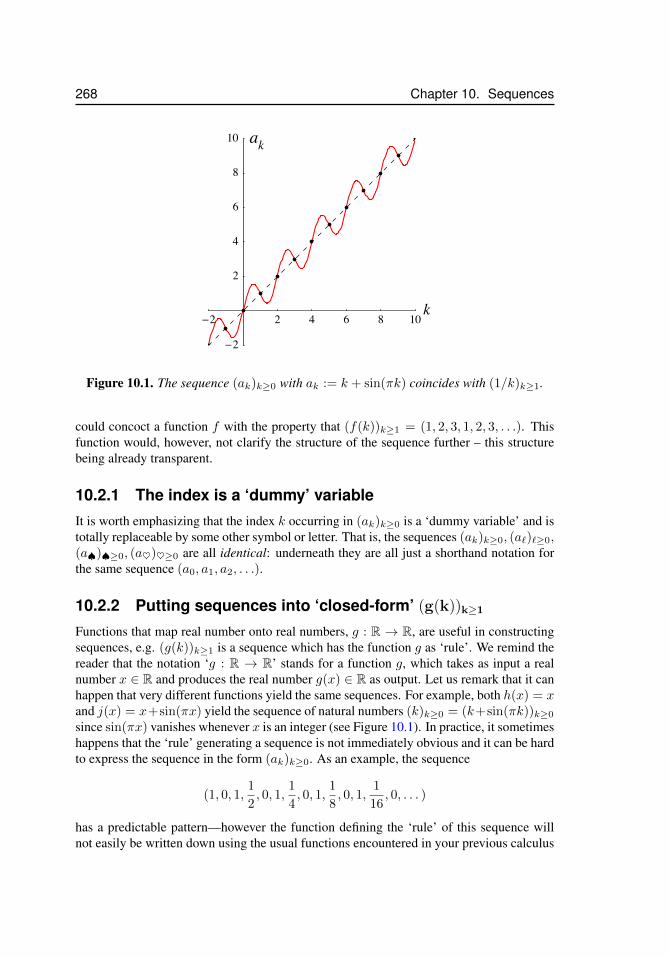
268 Chapter 10. Sequences
k!2 2 4 6 8 10
!2
2
4
6
8
10 ak
Figure 10.1. The sequence (ak)k≥0 with ak := k + sin(πk) coincides with (1/k)k≥1.
could concoct a function f with the property that (f(k))k≥1 = (1, 2, 3, 1, 2, 3, . . .). Thisfunction would, however, not clarify the structure of the sequence further – this structurebeing already transparent.
10.2.1 The index is a ‘dummy’ variableIt is worth emphasizing that the index k occurring in (ak)k≥0 is a ‘dummy variable’ and istotally replaceable by some other symbol or letter. That is, the sequences (ak)k≥0, (a`)`≥0,(a♠)♠≥0, (a♥)♥≥0 are all identical: underneath they are all just a shorthand notation forthe same sequence (a0, a1, a2, . . .).
10.2.2 Putting sequences into ‘closed-form’ (g(k))k≥1Functions that map real number onto real numbers, g : R → R, are useful in constructingsequences, e.g. (g(k))k≥1 is a sequence which has the function g as ‘rule’. We remind thereader that the notation ‘g : R → R’ stands for a function g, which takes as input a realnumber x ∈ R and produces the real number g(x) ∈ R as output. Let us remark that it canhappen that very different functions yield the same sequences. For example, both h(x) = xand j(x) = x+sin(πx) yield the sequence of natural numbers (k)k≥0 = (k+sin(πk))k≥0
since sin(πx) vanishes whenever x is an integer (see Figure 10.1). In practice, it sometimeshappens that the ‘rule’ generating a sequence is not immediately obvious and it can be hardto express the sequence in the form (ak)k≥0. As an example, the sequence
(1, 0, 1,1
2, 0, 1,
1
4, 0, 1,
1
8, 0, 1,
1
16, 0, . . . )
has a predictable pattern—however the function defining the ‘rule’ of this sequence willnot easily be written down using the usual functions encountered in your previous calculus
10.2. Sequences 269
courses. Hence although we understand the pattern generating the sequence (we could eas-ily write the first thousand terms of the sequence), it would be difficult to exhibit a functiondefining the sequence’s ‘rule’. Finding the ‘rule’ generating a sequence can be sometimes avery important problem: before one can run computer experiments on a sequence, one mustfirst know how to communicate the sequence to the computer. This will require knowingsome deterministic procedure to produce the sequence.
10.2.3 A trick questionLet us take a moment to get into some mischief: if we were feeling somewhat obnoxious,then we could pose the following ‘trick question’: “What are the next three terms t4, t5, t6in the sequence
(t1, t2, t3, . . .) := (1, 2, 3, . . .)?”
Of course, if we weren’t looking for mischief, then we would concede that t4 = 4, t5 = 5,t6 = 6, and that the sequence we had in mind was the expected (1, 2, 3, . . .) = (k)k≥1.However we could also claim that we really had the sequence (m(k))k≥1 in mind, wherewe deviantly defined the polynomial
m(x) =1
2(2− x)(3− x)− 2(1− x)(3− x) +
3
2(1− x)(2− x).
This yieldsCheck it!(m(k))k≥1 = (1, 2, 3,−14,−1, 6, . . .).
Most mathematicians (or calculus professors) are not so devilish nor have such a poor tastein jokes. Hence one can generally assume that the first terms of a sequence are writtenprecisely to aid the reader in discovering the ‘rule’ generating the sequence. So the readershould be at ease – the dots ‘. . .’ occurring in the sequence (1, 5, 9, 13, . . .) have a functionsimilar to the literary ‘etc’, meaning ‘and so forth’ or ‘continuing in the same way’, and, inthis case, gently direct towards the series (4k + 1)k≥0 = (1, 5, 9, 13, 17, 21, . . .).
10.2.4 Examples of SequencesThe following are among the basic examples of infinite sequences:
(i) the constant sequence (α, α, α, . . .) for any number α ∈ R.
(ii) the sequence of natural numbers: (0, 1, 2, . . .) = (n)n≥0;
(iii) the sequence of ‘harmonic numbers’: (1, 12 ,
13 , . . . ,
1n , . . .) = ( 1
k )k≥1.
(iv) the sequence of ‘geometric numbers’: (r0, r1, r2, r3, . . .) = (rk)k≥0 for any numberr ∈ R.
(v) an alternating sequence (+1,−1,+1,−1, . . .) = ((−1)k)k≥0;
These next sequences are perhaps a bit more curious:
(vi) the sequence (1, 1, 0, 1, 0, 0, 0, 1, 0, 0, 0, 0, 0, 0, 0, 1, . . .) = (εk)k≥1, where εk = 1whenever k is a power of 2, and εk = 0 otherwise.
270 Chapter 10. Sequences
(vii) the Fibonacci sequence (1, 1, 2, 3, 5, 8, 13, . . .) = (fn)n≥0, where f0, f1 = 1 andfk+2 := fk + fk+1 for k ≥ 0;
(viii) the sequence of squared integers (02, 12, 22, 32, . . .) = (0, 1, 4, 9, . . .) = (k2)k≥0;
(ix) Newton’s method yields the sequence (xk)k≥0 where xk+1 := xk − f(xk)f ′(xk) for a
differentiable function f : R→ R and a point x0 ∈ R (see section 10.5).
(x) Sequence of iterates (x0, f(x0), f(f(x0)), f(f(f(x0))), . . .), for any function f :R→ R and a point x0 ∈ R (see Section 10.6).
10.3 Convergent and Divergent SequencesConvergence and divergence are core concepts in mathematics (pure and applied) and thenatural sciences. One might say that a behaviour is convergent if, in the long-run, this be-haviour becomes fixed. Divergent behaviour is, in contrast, one which never settles. Ourinterests in convergence and divergence concern the long-time behaviour of sequences ofreal numbers. Our emphasis is on concrete examples and determining which basic se-quences converge or diverge.
We present two definitions of convergence. The first definition is a precise mathemat-ical statement – it is a piece of real mathematics that took over a hundred years to isolateand refine. However, we shall not require such sharp precision and thus present an alterna-tive, simpler and more intuitive formulation, which will serve as the working definition offor course.
Definition 3 (rigorous). The sequence (ak)k≥0 converges to the limit a∞ as k →∞ if, forany δ > 0, a number N(δ) exists such that for all values of k > N(δ), the |ak − a∞| < δholds.
The precise definition is provided for the simple reason to illustrate that rigorousmathematical definitions are not menacing. This concept of a convergent sequence is de-picted in Figure 10.2. Rephrasing Definition 3 in a more cavalier manner yields our work-ing definition:
Definition 4 (working version). An infinite sequence (ak)k≥0 converges to a∞ if for every‘error tolerance’ the terms ak of the sequence are eventually indistinguishable, i.e. liewithin that given error tolerance, from a∞.
In other words, regardless of any preassigned ‘error-tolerance’ the sequence (ak)k≥0
is eventually indistinguishable – up to that ‘error-tolerance’ – from the constant sequence(a∞, a∞, a∞, . . .).
The meaning of the expression ‘error tolerance’ requires clarification. How often dowe confuse the numbers 0 and 1 as being equal? One coffee mug rarely looks like no coffeemug. One 99 B-Line bus rarely looks like no 99 B-Line bus. On the other hand, one antvery often looks like no ant, and one coffee mug – as seen from a sufficiently far distance,say from the moon’s surface – will almost always look like no coffee mug. Our eyesight
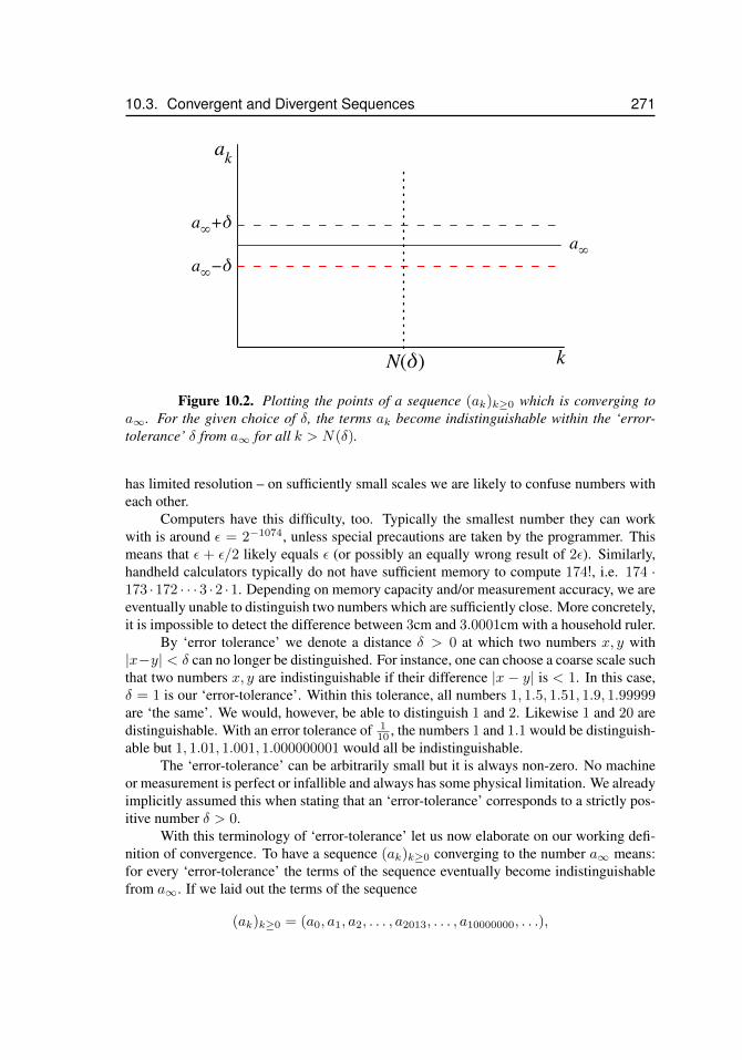
10.3. Convergent and Divergent Sequences 271
ak
k
a∞+δ
a∞−δa∞
N(δ)
Figure 10.2. Plotting the points of a sequence (ak)k≥0 which is converging toa∞. For the given choice of δ, the terms ak become indistinguishable within the ‘error-tolerance’ δ from a∞ for all k > N(δ).
has limited resolution – on sufficiently small scales we are likely to confuse numbers witheach other.
Computers have this difficulty, too. Typically the smallest number they can workwith is around ε = 2−1074, unless special precautions are taken by the programmer. Thismeans that ε + ε/2 likely equals ε (or possibly an equally wrong result of 2ε). Similarly,handheld calculators typically do not have sufficient memory to compute 174!, i.e. 174 ·173 ·172 · · · 3 ·2 ·1. Depending on memory capacity and/or measurement accuracy, we areeventually unable to distinguish two numbers which are sufficiently close. More concretely,it is impossible to detect the difference between 3cm and 3.0001cm with a household ruler.
By ‘error tolerance’ we denote a distance δ > 0 at which two numbers x, y with|x−y| < δ can no longer be distinguished. For instance, one can choose a coarse scale suchthat two numbers x, y are indistinguishable if their difference |x − y| is < 1. In this case,δ = 1 is our ‘error-tolerance’. Within this tolerance, all numbers 1, 1.5, 1.51, 1.9, 1.99999are ‘the same’. We would, however, be able to distinguish 1 and 2. Likewise 1 and 20 aredistinguishable. With an error tolerance of 1
10 , the numbers 1 and 1.1 would be distinguish-able but 1, 1.01, 1.001, 1.000000001 would all be indistinguishable.
The ‘error-tolerance’ can be arbitrarily small but it is always non-zero. No machineor measurement is perfect or infallible and always has some physical limitation. We alreadyimplicitly assumed this when stating that an ‘error-tolerance’ corresponds to a strictly pos-itive number δ > 0.
With this terminology of ‘error-tolerance’ let us now elaborate on our working defi-nition of convergence. To have a sequence (ak)k≥0 converging to the number a∞ means:for every ‘error-tolerance’ the terms of the sequence eventually become indistinguishablefrom a∞. If we laid out the terms of the sequence
(ak)k≥0 = (a0, a1, a2, . . . , a2013, . . . , a10000000, . . .),
272 Chapter 10. Sequences
and if we saw ourselves ‘walking along’ with the terms of the sequence, i.e. walkingfrom the first term to the second, to the third, fourth, etc., then there would be a termin the sequence (a point in time during our walk) after which all future terms would beindistinguishable within our ‘error-tolerance’ from a∞. In Definition 3 this term (or ‘point-in-time’) corresponds to N(δ). Note that for a smaller ‘error tolerance’, δ′ with δ > δ′ > 0then N(δ) ≤ N(δ′). In other words, a finer ‘error-tolerance’ will require us to walk furtheralong the sequence before the terms become indistinguishable.
A basic example of a convergent sequence in which the δ’s and N(δ)’s can be madetotally explicit is in the harmonic sequence (1/n)n≥0 with limn→∞ 1/n = 0. For anychoice of δ > 0 we can set N(δ) = 1/δ. Thus for δ very small, N(δ) = 1/δ will be verylarge. All this follows from seeing that 1/n < δ if and only if n > 1/δ.
Notation
If a sequence (ak)k≥0 converges to the limit a∞, we write
limk→∞
ak = a∞,
or for brevity, if there is no ambiguity, simply
ak → a∞.
The expression k →∞ means “as k tends to∞”.A sequence (ak)k≥0 is divergent if it does not converge to any real number. More
precisely, for every real number L there exists δ > 0 such that infinitely many terms in thesequence differ from L by more than δ. Or, negating the above definitions of convergence,divergence means that for some ’error-tolerances’, δ, some terms in the sequence will al-ways differ from any a∞ by more than δ, no matter how far we walk along the sequence.
Terminology
When describing sequences, the following terminology is useful:
(i) A sequence (ak)k≥0 is bounded if there exists a number M > 0 such that |ak| ≤ Mfor all k ≥ 0.
(ii) A sequence (ak)k≥0 is monotone or monotonic if either (i) a0 ≤ a1 ≤ a2 ≤ . . . or(ii) a0 ≥ a1 ≥ a2 ≥ . . .; in case (i) we say the sequence is monotonically increasing,and in case (ii) it is monotonically decreasing.
For example, the sequence
(i) ( 1k )k≥1 is bounded by M = 1 (actually any M ≥ 1) and monotonically decreasing;
(ii) (cos(πk ))k≥1 is bounded by M = 1 and monotonically increasing;
(iii) ( (−1)k
k2 )k≥1 is bounded by M = 1 and is not monotonic;
(iv) of natural numbers (1, 2, 3, . . .) is not bounded and is monotonically increasing;
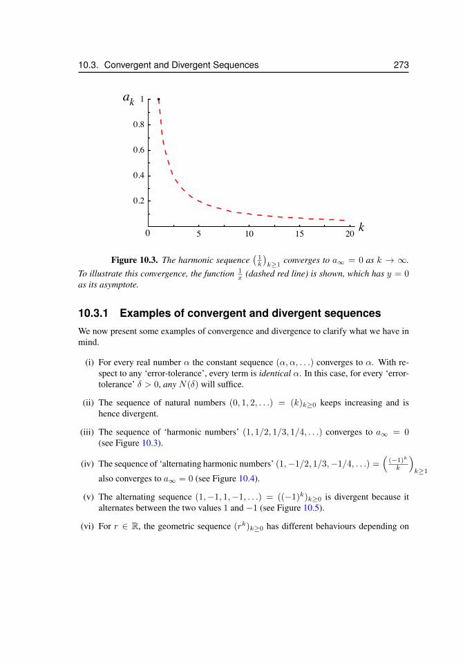
10.3. Convergent and Divergent Sequences 273
5 10 15 20
0.2
0.4
0.6
0.8
1
k
ak
0
Figure 10.3. The harmonic sequence(
1k
)k≥1
converges to a∞ = 0 as k → ∞.To illustrate this convergence, the function 1
x (dashed red line) is shown, which has y = 0as its asymptote.
10.3.1 Examples of convergent and divergent sequencesWe now present some examples of convergence and divergence to clarify what we have inmind.
(i) For every real number α the constant sequence (α, α, . . .) converges to α. With re-spect to any ‘error-tolerance’, every term is identical α. In this case, for every ‘error-tolerance’ δ > 0, any N(δ) will suffice.
(ii) The sequence of natural numbers (0, 1, 2, . . .) = (k)k≥0 keeps increasing and ishence divergent.
(iii) The sequence of ‘harmonic numbers’ (1, 1/2, 1/3, 1/4, . . .) converges to a∞ = 0(see Figure 10.3).
(iv) The sequence of ‘alternating harmonic numbers’ (1,−1/2, 1/3,−1/4, . . .) =(
(−1)k
k
)k≥1
also converges to a∞ = 0 (see Figure 10.4).
(v) The alternating sequence (1,−1, 1,−1, . . .) = ((−1)k)k≥0 is divergent because italternates between the two values 1 and −1 (see Figure 10.5).
(vi) For r ∈ R, the geometric sequence (rk)k≥0 has different behaviours depending on
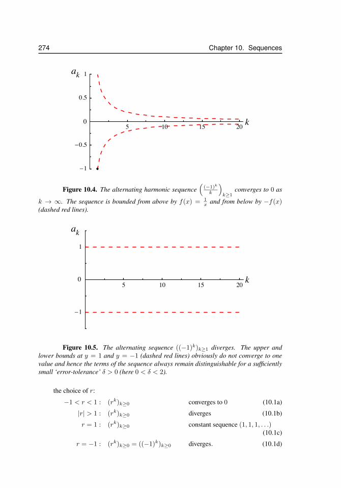
274 Chapter 10. Sequences
5 10 15 20
!1
!0.5
0.5
1
k
ak
0
Figure 10.4. The alternating harmonic sequence(
(−1)k
k
)k≥1
converges to 0 as
k → ∞. The sequence is bounded from above by f(x) = 1x and from below by −f(x)
(dashed red lines).
5 10 15 20
!1
1
k
ak
0
Figure 10.5. The alternating sequence ((−1)k)k≥1 diverges. The upper andlower bounds at y = 1 and y = −1 (dashed red lines) obviously do not converge to onevalue and hence the terms of the sequence always remain distinguishable for a sufficientlysmall ‘error-tolerance’ δ > 0 (here 0 < δ < 2).
the choice of r:
−1 < r < 1 : (rk)k≥0 converges to 0 (10.1a)
|r| > 1 : (rk)k≥0 diverges (10.1b)
r = 1 : (rk)k≥0 constant sequence (1, 1, 1, . . .)(10.1c)
r = −1 : (rk)k≥0 = ((−1)k)k≥0 diverges. (10.1d)
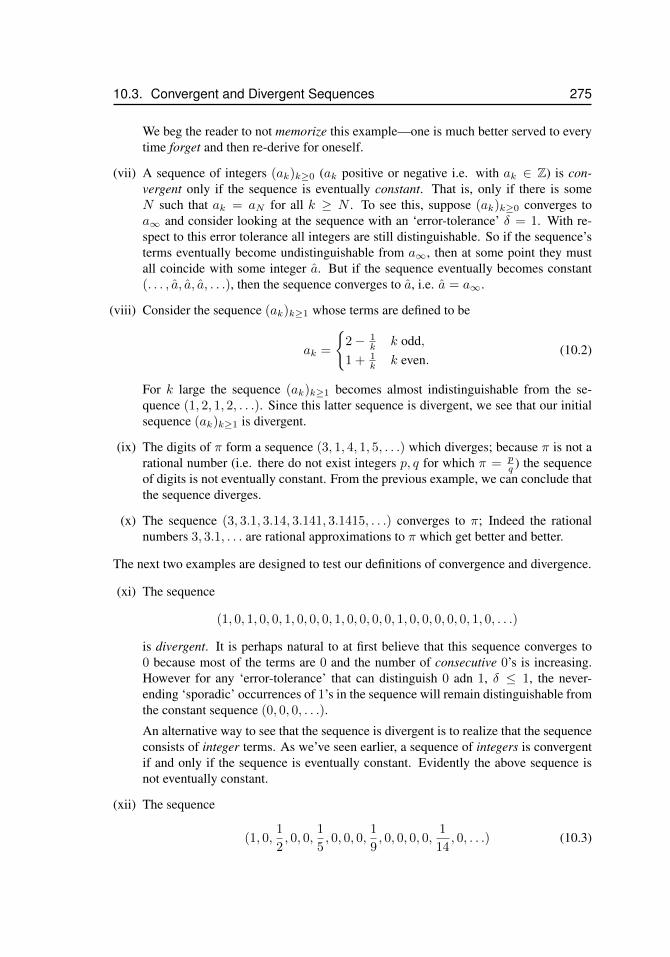
10.3. Convergent and Divergent Sequences 275
We beg the reader to not memorize this example—one is much better served to everytime forget and then re-derive for oneself.
(vii) A sequence of integers (ak)k≥0 (ak positive or negative i.e. with ak ∈ Z) is con-vergent only if the sequence is eventually constant. That is, only if there is someN such that ak = aN for all k ≥ N . To see this, suppose (ak)k≥0 converges toa∞ and consider looking at the sequence with an ‘error-tolerance’ δ = 1. With re-spect to this error tolerance all integers are still distinguishable. So if the sequence’sterms eventually become undistinguishable from a∞, then at some point they mustall coincide with some integer a. But if the sequence eventually becomes constant(. . . , a, a, a, . . .), then the sequence converges to a, i.e. a = a∞.
(viii) Consider the sequence (ak)k≥1 whose terms are defined to be
ak =
{2− 1
k k odd,1 + 1
k k even.(10.2)
For k large the sequence (ak)k≥1 becomes almost indistinguishable from the se-quence (1, 2, 1, 2, . . .). Since this latter sequence is divergent, we see that our initialsequence (ak)k≥1 is divergent.
(ix) The digits of π form a sequence (3, 1, 4, 1, 5, . . .) which diverges; because π is not arational number (i.e. there do not exist integers p, q for which π = p
q ) the sequenceof digits is not eventually constant. From the previous example, we can conclude thatthe sequence diverges.
(x) The sequence (3, 3.1, 3.14, 3.141, 3.1415, . . .) converges to π; Indeed the rationalnumbers 3, 3.1, . . . are rational approximations to π which get better and better.
The next two examples are designed to test our definitions of convergence and divergence.
(xi) The sequence
(1, 0, 1, 0, 0, 1, 0, 0, 0, 1, 0, 0, 0, 0, 1, 0, 0, 0, 0, 0, 1, 0, . . .)
is divergent. It is perhaps natural to at first believe that this sequence converges to0 because most of the terms are 0 and the number of consecutive 0’s is increasing.However for any ‘error-tolerance’ that can distinguish 0 adn 1, δ ≤ 1, the never-ending ‘sporadic’ occurrences of 1’s in the sequence will remain distinguishable fromthe constant sequence (0, 0, 0, . . .).
An alternative way to see that the sequence is divergent is to realize that the sequenceconsists of integer terms. As we’ve seen earlier, a sequence of integers is convergentif and only if the sequence is eventually constant. Evidently the above sequence isnot eventually constant.
(xii) The sequence
(1, 0,1
2, 0, 0,
1
5, 0, 0, 0,
1
9, 0, 0, 0, 0,
1
14, 0, . . .) (10.3)
276 Chapter 10. Sequences
converges to 0. We know the sequence (1, 12 ,
15 ,
19 , . . .) converges to 0 – for example
because each term is smaller than that of the converging harmonic series (see Fig-ure 10.3). This means that regardless of any prescribed ‘error-tolerance’, the sequenceeventually becomes indistinguishable from the constant zero sequence (0, 0, 0, . . .).Likewise, our sequence (10.3) will eventually become indistinguishable from the con-stant zero sequence and hence converges.
While the sequence (10.3) has never-ending sporadic occurrences of nonzero positivenumbers, the magnitude of these ‘outbursts’ are decaying. Very far into the sequence,say after the ten millionth term, these sporadic outbursts are just ‘whispers’ – they arevery nearly zeros themselves.
10.3.2 The ‘head’ of a sequence does not affect convergenceFor any sequence (ak)k≥0 the first, say, million terms can be altered without altering eitherits convergence or divergence. Moreover, if the original sequence converges to a numbera∞, then any sequence obtained by altering, again say, the first million terms, yields anothersequence but still converging to a∞. The convergence or divergence of a sequence is astatement about its terms ‘ad infinitum’, i.e. in the (infinitely) long run.
It is perhaps helpful to consider sequences, (ak)k≥0, as having two parts: a head anda tail. The finite sequence (a0, . . . , ak) the is called the head, and the infinite sequence(ak, ak+1, ak+2, . . .) the tail. A sequence is like a worm stretching from your feet to thehorizon. Every segment of the worm’s torso contains a number. A choice of segment, ak(choice of worm-saddle), then determines the head and tail of the worm. The head is thefinite part in front of the saddle, and the tail is the infinite part trailing behind the saddle.Convergence concerns only the tail, i.e. what happens to those numbers on the torso as wemove further along the worm towards the horizon.
10.3.3 Sequences and Horizontal Asymptotes of FunctionsOur discussion of convergent and divergent sequences should invoke some memories ofyour differential calculus course and similar discussions in relation to functions. The verydefinition of derivative itself requires the convergence of a sequence of secants, i.e. thederivative was originally defined by Newton as the limit
limx→a
f(x)− f(a)
x− a=: f ′(a).
Alternatively we could use the recipe: tangent = lim secants. Here we briefly show howyour previous experience with functions and limits can be used in understanding convergentsequences.
If the terms in a sequence (ak)k≥0 have the form ak = f(k) for some function f(x)then the sequence converges if and only if the function f(x) has a horizontal asymptote asx→ +∞. Specifically, if limx→∞ f(x) = L, then ak → L.
As an example, consider the function f(x) = 2x3−1x3+1 , which has the line y = 2 as
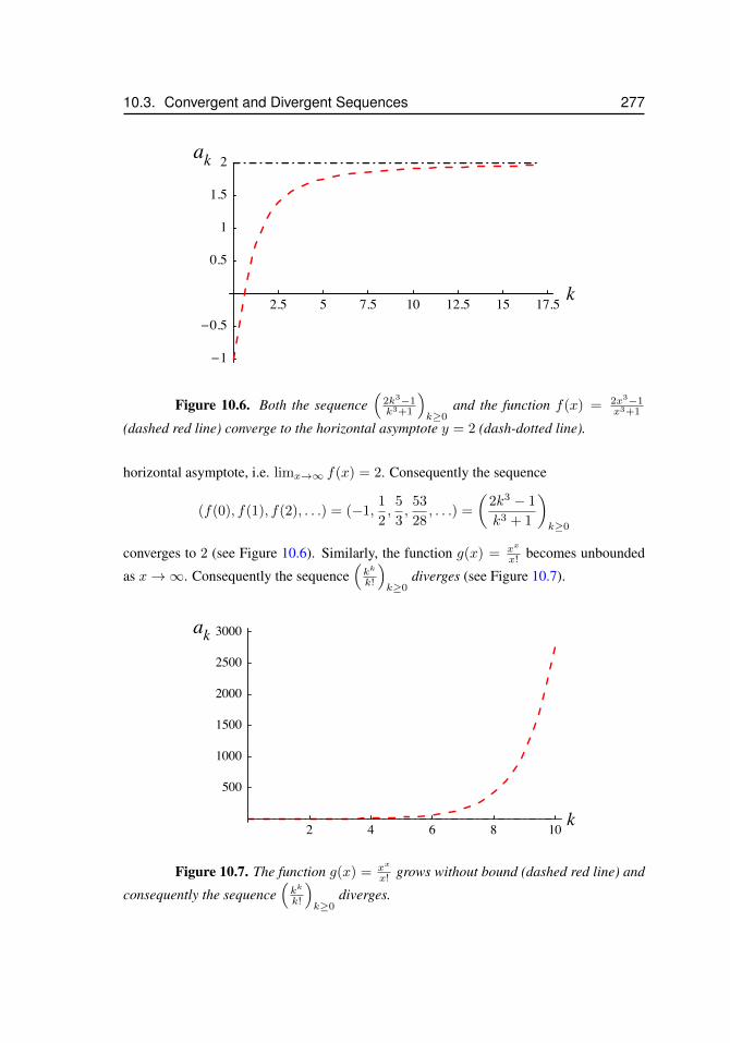
10.3. Convergent and Divergent Sequences 277
2.5 5 7.5 10 12.5 15 17.5
!1
!0.5
0.5
1
1.5
2
k
ak
Figure 10.6. Both the sequence(
2k3−1k3+1
)k≥0
and the function f(x) = 2x3−1x3+1
(dashed red line) converge to the horizontal asymptote y = 2 (dash-dotted line).
horizontal asymptote, i.e. limx→∞ f(x) = 2. Consequently the sequence
(f(0), f(1), f(2), . . .) = (−1,1
2,
5
3,
53
28, . . .) =
(2k3 − 1
k3 + 1
)k≥0
converges to 2 (see Figure 10.6). Similarly, the function g(x) = xx
x! becomes unbounded
as x→∞. Consequently the sequence(kk
k!
)k≥0
diverges (see Figure 10.7).
2 4 6 8 10
500
1000
1500
2000
2500
3000
k
ak
Figure 10.7. The function g(x) = xx
x! grows without bound (dashed red line) and
consequently the sequence(kk
k!
)k≥0
diverges.
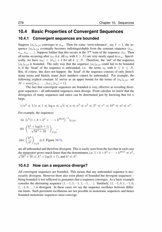
278 Chapter 10. Sequences
10.4 Basic Properties of Convergent Sequences10.4.1 Convergent sequences are boundedSuppose (ak)k≥0 converges to a∞. Then for some ‘error-tolerance’, say δ = 1, the se-quence (ak)k≥0 eventually becomes indistinguishable from the constant sequence (a∞,a∞, a∞, . . .). Suppose further that this occurs at the N th term of the sequence, aN . Thenall terms occurring after aN (i.e. all ak with k > N ) are very nearly equal to a∞. Specif-ically, we have |ak| < |a∞| + δ for all k ≥ N . Therefore, the ‘tail’ of the sequence(ak)k≥0 is bounded. The only way that the sequence (ak)k≥0 could fail to be boundedis if the ‘head’ of the sequence is unbounded, i.e. the terms ak with 0 ≤ k ≤ N .But, of course, this does not happen: the ‘head’ of the sequence consists of only finitelymany terms and finitely many finite numbers cannot be unbounded. For example, thefollowing explicit constant M serves as an upper bound for the terms of (ak)k≥0: setM = max{|a1|, . . . , |aN |, |a∞|+ 1}.
The fact that convergent sequences are bounded is very effective at revealing diver-gent sequences – all unbounded sequences must diverge. From calculus we know that thedivergence of many sequences and ratios can be determined just by knowing that for nlarge,
1/n2 � 1/n� 1� log n�√n� n� n2 � n3 � 2n � en � 10n � n!� nn.
For example, the sequences
(i)(ek(1 + k + k2 + · · ·+ k2013
)−1)k≥0,
(ii)(k4 + log(k + 1)√
5k7 + 16
)k≥0
,
(iii)(kk
k!
)k≥0
(c.f. Figure 10.7),
are all unbounded and therefore divergent. This is easily seen from the fact that in each casethe numerator grows much faster than the denominator, i.e. 1+k+k2 + · · ·+k2013 � ek,√
5k7 + 16� k4 + log(k + 1), and k!� kk.
10.4.2 How can a sequence diverge?All convergent sequences are bounded. This means that any unbounded sequence is nec-essarily divergent. However there also exist plenty of bounded but divergent sequences –being bounded is not sufficient to guarantee that a sequence converges. As a basic exampleconsider the alternating sequence (1,−1, 1,−1, 1,−1, . . .). Similarly, (1,−1, 0, 1,−1, 0,1,−1, 0, . . .) is divergent. In these cases we say the sequence oscillates between differ-ent limits. Such persistent oscillations are not possible in monotonic sequences and hencebounded monotonic sequences must converge.
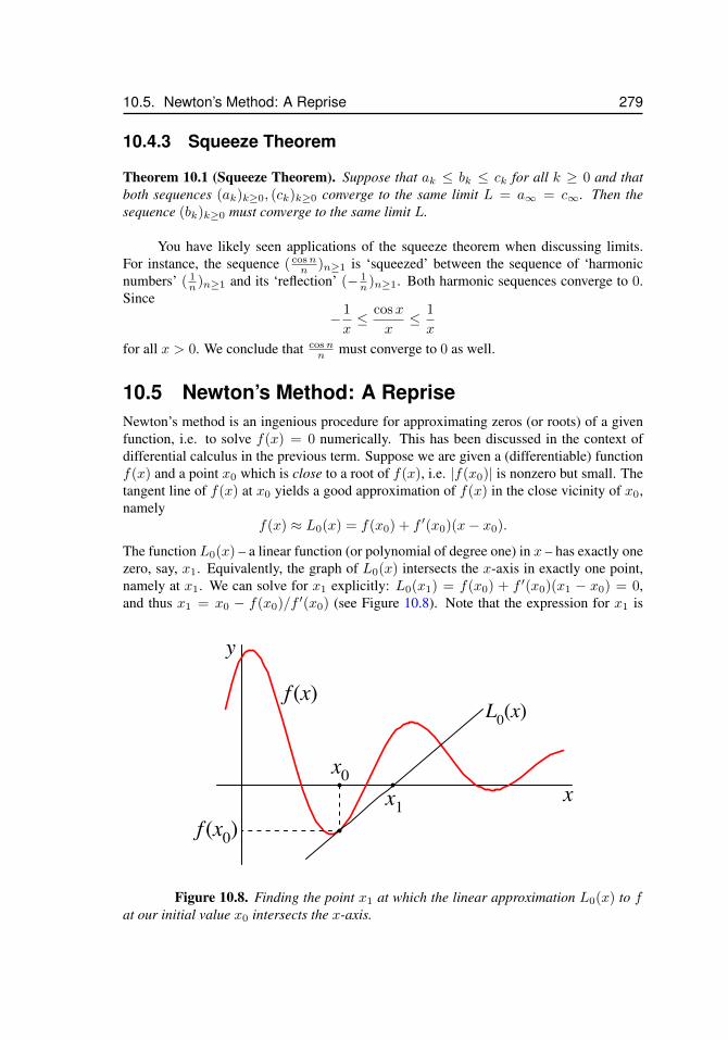
10.5. Newton’s Method: A Reprise 279
10.4.3 Squeeze Theorem
Theorem 10.1 (Squeeze Theorem). Suppose that ak ≤ bk ≤ ck for all k ≥ 0 and thatboth sequences (ak)k≥0, (ck)k≥0 converge to the same limit L = a∞ = c∞. Then thesequence (bk)k≥0 must converge to the same limit L.
You have likely seen applications of the squeeze theorem when discussing limits.For instance, the sequence ( cosn
n )n≥1 is ‘squeezed’ between the sequence of ‘harmonicnumbers’ ( 1
n )n≥1 and its ‘reflection’ (− 1n )n≥1. Both harmonic sequences converge to 0.
Since− 1
x≤ cosx
x≤ 1
x
for all x > 0. We conclude that cosnn must converge to 0 as well.
10.5 Newton’s Method: A RepriseNewton’s method is an ingenious procedure for approximating zeros (or roots) of a givenfunction, i.e. to solve f(x) = 0 numerically. This has been discussed in the context ofdifferential calculus in the previous term. Suppose we are given a (differentiable) functionf(x) and a point x0 which is close to a root of f(x), i.e. |f(x0)| is nonzero but small. Thetangent line of f(x) at x0 yields a good approximation of f(x) in the close vicinity of x0,namely
f(x) ≈ L0(x) = f(x0) + f ′(x0)(x− x0).
The function L0(x) – a linear function (or polynomial of degree one) in x – has exactly onezero, say, x1. Equivalently, the graph of L0(x) intersects the x-axis in exactly one point,namely at x1. We can solve for x1 explicitly: L0(x1) = f(x0) + f ′(x0)(x1 − x0) = 0,and thus x1 = x0 − f(x0)/f ′(x0) (see Figure 10.8). Note that the expression for x1 is
x
y
f (x)
x0
f (x0)x1
L0(x)
Figure 10.8. Finding the point x1 at which the linear approximation L0(x) to fat our initial value x0 intersects the x-axis.
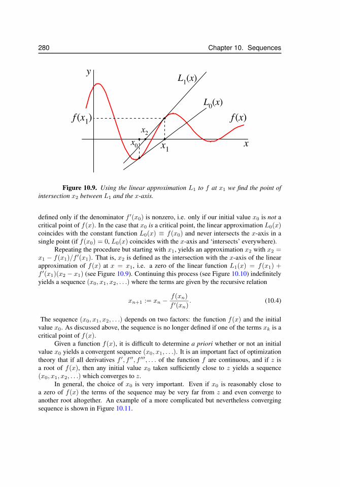
280 Chapter 10. Sequences
x
y
f (x)
x0
f (x1)
x1
x2
L0(x)
L1(x)
Figure 10.9. Using the linear approximation L1 to f at x1 we find the point ofintersection x2 between L1 and the x-axis.
defined only if the denominator f ′(x0) is nonzero, i.e. only if our initial value x0 is not acritical point of f(x). In the case that x0 is a critical point, the linear approximation L0(x)coincides with the constant function L0(x) ≡ f(x0) and never intersects the x-axis in asingle point (if f(x0) = 0, L0(x) coincides with the x-axis and ‘intersects’ everywhere).
Repeating the procedure but starting with x1, yields an approximation x2 with x2 =x1 − f(x1)/f ′(x1). That is, x2 is defined as the intersection with the x-axis of the linearapproximation of f(x) at x = x1, i.e. a zero of the linear function L1(x) = f(x1) +f ′(x1)(x2 − x1) (see Figure 10.9). Continuing this process (see Figure 10.10) indefinitelyyields a sequence (x0, x1, x2, . . .) where the terms are given by the recursive relation
xn+1 := xn −f(xn)
f ′(xn). (10.4)
The sequence (x0, x1, x2, . . .) depends on two factors: the function f(x) and the initialvalue x0. As discussed above, the sequence is no longer defined if one of the terms xk is acritical point of f(x).
Given a function f(x), it is difficult to determine a priori whether or not an initialvalue x0 yields a convergent sequence (x0, x1, . . .). It is an important fact of optimizationtheory that if all derivatives f ′, f ′′, f ′′′, . . . of the function f are continuous, and if z isa root of f(x), then any initial value x0 taken sufficiently close to z yields a sequence(x0, x1, x2, . . .) which converges to z.
In general, the choice of x0 is very important. Even if x0 is reasonably close toa zero of f(x) the terms of the sequence may be very far from z and even converge toanother root altogether. An example of a more complicated but nevertheless convergingsequence is shown in Figure 10.11.
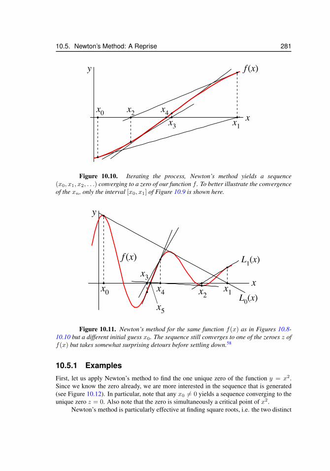
10.5. Newton’s Method: A Reprise 281
x
y f (x)
x0x1
x2x3
x4
Figure 10.10. Iterating the process, Newton’s method yields a sequence(x0, x1, x2, . . .) converging to a zero of our function f . To better illustrate the convergenceof the xn, only the interval [x0, x1] of Figure 10.9 is shown here.
x
y
f (x)
x0L0(x)
L1(x)
x1x2
x3
x5
x4
Figure 10.11. Newton’s method for the same function f(x) as in Figures 10.8-10.10 but a different initial guess x0. The sequence still converges to one of the zeroes z off(x) but takes somewhat surprising detours before settling down.58
10.5.1 ExamplesFirst, let us apply Newton’s method to find the one unique zero of the function y = x2.Since we know the zero already, we are more interested in the sequence that is generated(see Figure 10.12). In particular, note that any x0 6= 0 yields a sequence converging to theunique zero z = 0. Also note that the zero is simultaneously a critical point of x2.
Newton’s method is particularly effective at finding square roots, i.e. the two distinct
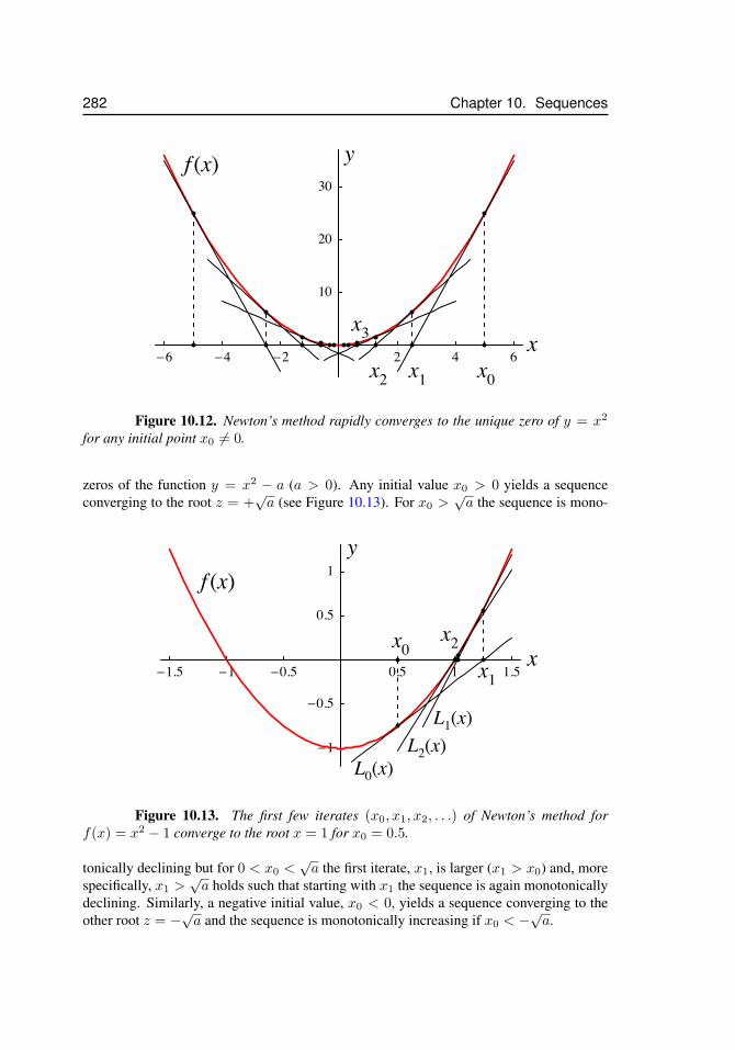
282 Chapter 10. Sequences
!6 !4 !2 2 4 6
10
20
30
x0x1x2
x3 x
yf (x)
Figure 10.12. Newton’s method rapidly converges to the unique zero of y = x2
for any initial point x0 6= 0.
zeros of the function y = x2 − a (a > 0). Any initial value x0 > 0 yields a sequenceconverging to the root z = +
√a (see Figure 10.13). For x0 >
√a the sequence is mono-
!1.5 !1 !0.5 0.5 1 1.5
!1
!0.5
0.5
1
x
yf (x)
x0x1
x2
L0(x)
L1(x)L2(x)
Figure 10.13. The first few iterates (x0, x1, x2, . . .) of Newton’s method forf(x) = x2 − 1 converge to the root x = 1 for x0 = 0.5.
tonically declining but for 0 < x0 <√a the first iterate, x1, is larger (x1 > x0) and, more
specifically, x1 >√a holds such that starting with x1 the sequence is again monotonically
declining. Similarly, a negative initial value, x0 < 0, yields a sequence converging to theother root z = −
√a and the sequence is monotonically increasing if x0 < −
√a.
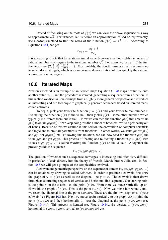
10.6. Iterated Maps 283
Instead of focussing on the roots of f(x) we can view the above sequence as a wayto approximate
√a. For instance, let us derive an approximation of
√3 or, equivalently,
use Newton’s method to find the zeros of the function f(x) = x2 − 3. According toEquation (10.4) we get
xk+1 =x2k + 3
2xk.
It is interesting to note that for a rational initial value, Newton’s method yields a sequence ofrational numbers converging to the irrational number
√3. For example, for x0 = 2 the first
few terms are (2, 74 ,
9756 ,
1881710864 , . . .). Most notably, the fourth term is already accurate up
to seven decimal digits, which is an impressive demonstration of how quickly the rationalapproximation converges.
10.6 Iterated MapsNewton’s method is an example of an iterated map: Equation (10.4) maps a value xk ontoanother value xk+1 and the procedure is iterated, generating a sequence from a function. Inthis section we discuss iterated maps from a slightly more general perspective and introducean interesting and fun technique to graphically generate sequences based on iterated maps,called cobwebs.
To begin, pick your favourite function g = g(x) and your favourite real number v.Evaluating the function g(x) at the value v then yields g(v) – some other number, whichtypically is different from our initial v. Now we can feed the function g(x) this new valueg(v) to obtain g(g(v)). If we keep doing this the number of brackets involved gets easily outof hands. Because of this we assume in this section the convention of computer scientistsand logicians to omit all parenthesis from functions. In other words, we write gv for g(v)and ggv for g(g(v)) etc. Following this notation, we can now feed the function g(x) thevalue ggv and get gggv. This process of feeding and re-feeding a function g = g(x) withvalues v, gv, ggv, . . . is called iterating the function g(x) on the value v. Altogether theprocess yields the sequence
(v, gv, ggv, gggv, . . .).
The question of whether such a sequence converges is interesting and often very difficult.In particular, it leads directly into the theory of fractals, Mandelbrot & Julia sets. In Sec-tion 10.8 we will get a glimpse of the complexities involved.
A convenient geometric perspective on the sequence of iterates (v, gv, ggv, gggv, . . .)can be obtained by drawing so-called cobwebs. In order to produce a cobweb, first drawthe graph of y = g(x) as well as the diagonal line y = x. The cobweb is then drawnthrough an alternating sequence of vertical and horizontal line segments. Our starting pointis the point v on the x-axis, i.e. the point (v, 0). From there we move vertically up un-til we hit the graph of g(x). This is the point (v, gv). Now we move horizontally untilwe reach the diagonal line at the point (gv, gv). These are the first two segments of yourcobweb (see Figure 10.14a). Next we move again vertically to the graph g(x) to find thepoint (gv, ggv) and then horizontally to meet the diagonal at the point (ggv, ggv) (seeFigure 10.14b). This process is iterated (see Figure 10.14c, d): vertical to (ggv, gggv),horizontal to (gggv, gggv), vertical to (gggv, ggggv) etc.
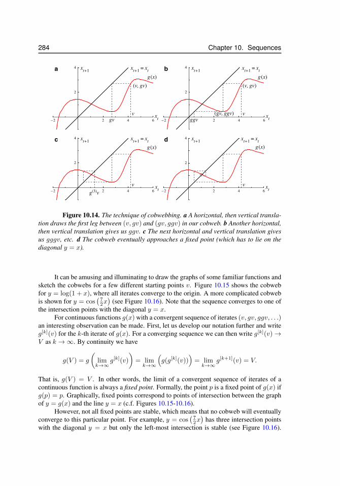
284 Chapter 10. Sequences
!2 2 4 6
2
4
vgv
(v, gv)
xt
xt+1 xt+1 = xtg (x)
!2 2 4 6
2
4
(v, gv)
(gv, ggv)ggv
v xt
xt+1 xt+1 = xtg (x)
!2 2 4 6
2
4
g(3)vv xt
xt+1 xt+1 = xtg (x)
!2 2 4 6
2
4
v xt
xt+1 xt+1 = xtg (x)
a b
c d
Figure 10.14. The technique of cobwebbing. a A horizontal, then vertical transla-tion draws the first leg between (v, gv) and (gv, ggv) in our cobweb. b Another horizontal,then vertical translation gives us ggv. c The next horizontal and vertical translation givesus gggv, etc. d The cobweb eventually approaches a fixed point (which has to lie on thediagonal y = x).
It can be amusing and illuminating to draw the graphs of some familiar functions andsketch the cobwebs for a few different starting points v. Figure 10.15 shows the cobwebfor y = log(1 + x), where all iterates converge to the origin. A more complicated cobwebis shown for y = cos
(72x)
(see Figure 10.16). Note that the sequence converges to one ofthe intersection points with the diagonal y = x.
For continuous functions g(x) with a convergent sequence of iterates (v, gv, ggv, . . .)an interesting observation can be made. First, let us develop our notation further and writeg[k](v) for the k-th iterate of g(x). For a converging sequence we can then write g[k](v)→V as k →∞. By continuity we have
g(V ) = g
(limk→∞
g[k](v)
)= limk→∞
(g(g[k](v))
)= limk→∞
g[k+1](v) = V.
That is, g(V ) = V . In other words, the limit of a convergent sequence of iterates of acontinuous function is always a fixed point. Formally, the point p is a fixed point of g(x) ifg(p) = p. Graphically, fixed points correspond to points of intersection between the graphof y = g(x) and the line y = x (c.f. Figures 10.15-10.16).
However, not all fixed points are stable, which means that no cobweb will eventuallyconverge to this particular point. For example, y = cos
(72x)
has three intersection pointswith the diagonal y = x but only the left-most intersection is stable (see Figure 10.16).
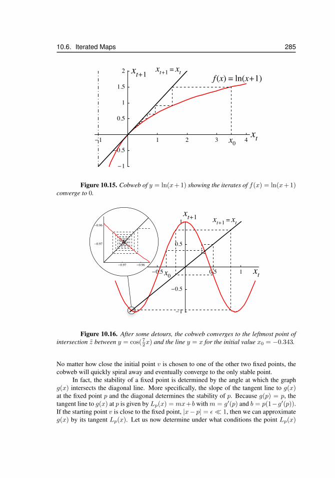
10.6. Iterated Maps 285
!1 1 2 3 4
!1
!0.5
0.5
1
1.5
2 xt+1
xt
f (x) = ln(x+1)
x0
xt+1 = xt
Figure 10.15. Cobweb of y = ln(x+ 1) showing the iterates of f(x) = ln(x+ 1)converge to 0.
!1 !0.5 0.5 1
!1
!0.5
0.5
1
!0.97 !0.96
!0.97
!0.96
xt
xt+1 xt+1 = xt
x0
Figure 10.16. After some detours, the cobweb converges to the leftmost point ofintersection z between y = cos( 7
2x) and the line y = x for the initial value x0 = −0.343.
No matter how close the initial point v is chosen to one of the other two fixed points, thecobweb will quickly spiral away and eventually converge to the only stable point.
In fact, the stability of a fixed point is determined by the angle at which the graphg(x) intersects the diagonal line. More specifically, the slope of the tangent line to g(x)at the fixed point p and the diagonal determines the stability of p. Because g(p) = p, thetangent line to g(x) at p is given by Lp(x) = mx+b withm = g′(p) and b = p(1−g′(p)).If the starting point v is close to the fixed point, |x− p| = ε� 1, then we can approximateg(x) by its tangent Lp(x). Let us now determine under what conditions the point Lp(x)
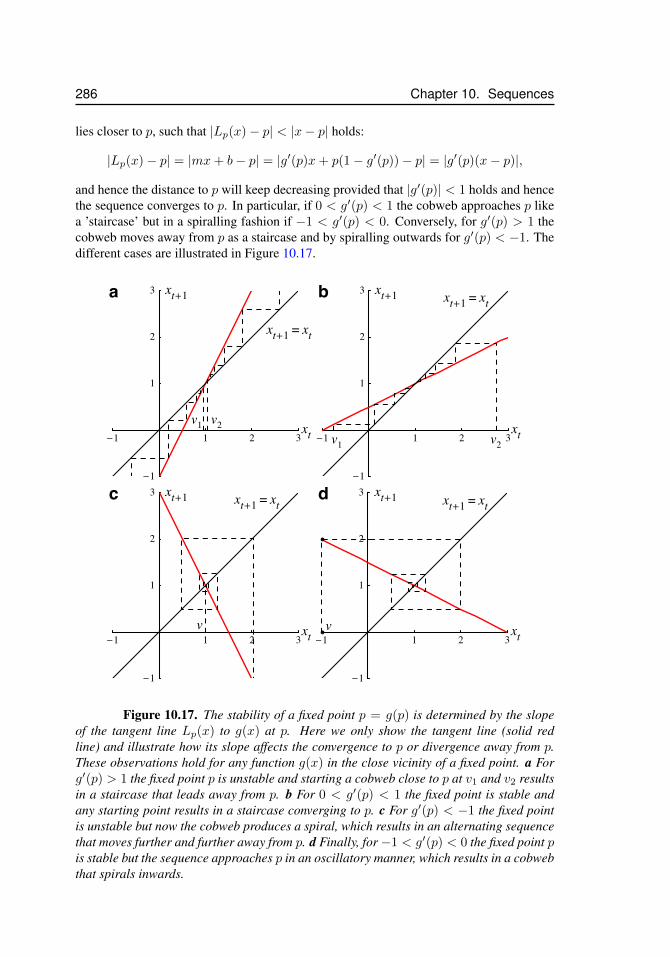
286 Chapter 10. Sequences
lies closer to p, such that |Lp(x)− p| < |x− p| holds:
|Lp(x)− p| = |mx+ b− p| = |g′(p)x+ p(1− g′(p))− p| = |g′(p)(x− p)|,
and hence the distance to p will keep decreasing provided that |g′(p)| < 1 holds and hencethe sequence converges to p. In particular, if 0 < g′(p) < 1 the cobweb approaches p likea ’staircase’ but in a spiralling fashion if −1 < g′(p) < 0. Conversely, for g′(p) > 1 thecobweb moves away from p as a staircase and by spiralling outwards for g′(p) < −1. Thedifferent cases are illustrated in Figure 10.17.
!1 1 2 3
!1
1
2
3xt+1 = xt
xt
xt+1
v
!1 1 2 3
!1
1
2
3
xt+1 = xt
xt
xt+1
v1 v2
a
!1 1 2 3
!1
1
2
3 xt+1 = xt
xt
xt+1
v1 v2
b
!1 1 2 3
!1
1
2
3 xt+1 = xt
xt
xt+1
v
c d
Figure 10.17. The stability of a fixed point p = g(p) is determined by the slopeof the tangent line Lp(x) to g(x) at p. Here we only show the tangent line (solid redline) and illustrate how its slope affects the convergence to p or divergence away from p.These observations hold for any function g(x) in the close vicinity of a fixed point. a Forg′(p) > 1 the fixed point p is unstable and starting a cobweb close to p at v1 and v2 resultsin a staircase that leads away from p. b For 0 < g′(p) < 1 the fixed point is stable andany starting point results in a staircase converging to p. c For g′(p) < −1 the fixed pointis unstable but now the cobweb produces a spiral, which results in an alternating sequencethat moves further and further away from p. d Finally, for−1 < g′(p) < 0 the fixed point pis stable but the sequence approaches p in an oscillatory manner, which results in a cobwebthat spirals inwards.
10.7. Difference Equations 287
A function may not have any fixed points, i.e. does not intersect the diagonal line,and even if it does, the fixed point may not be stable. Only functions that have at leastone stable fixed point can yield convergent sequences at least for some starting points. Thecobweb of a convergent sequence is bounded but not all bounded cobwebs are convergent.Just as diverging bounded sequences must have two or more subsequences that convergeto different limits, bounded cobwebs that do not converge must visit two or more pointsrepeatedly – this gives rise to periodic cycles. A topic that will be briefly addressed in thenext section in the context of population dynamics.
10.7 Difference EquationsModelling the dynamics of populations is among the most basic problems in theoreticalecology. Let the number of individuals in a population at time t be Nt. If, in one unit oftime, every individual produces, on average, α offspring then the population size at timet+ 1 is given by
Nt+1 = αNt. (10.5)
Note that Nt does not need to be an integer number – it represents the average or expectednumber of individuals in the population. Also note that in sexual populations a simpletrick is to count only females because the production of eggs and/or the gestation periodusually present the limiting factors for population growth. If the sex ratio is known for thespecies under consideration then it is straight forward to determine the entire populationsize. Equation (10.5) is the simplest difference equation. More specifically, the differencein population size at time t and t+ 1 is given by
Nt+1 −Nt = (α− 1)Nt.
Instead of incrementing the time by one unit, we could, for example, increment the time by∆t and get
Nt+∆t −Nt = (α∆t − 1)Nt.
Note that α is the (net) number of offspring per unit time and so there are α∆t offspring inthe time interval ∆t. Now we can divide both sides by ∆t and take the limit ∆t → 0 torecover the differential equation
d
dtN(t) = ln(α)N(t), (10.6)
where we have used de l’Hopital’s rule to calculate the right hand limit. In this limit, thenumber of offspring per individual (or per capita, i.e. per ‘head’) per time step,Nt+1/Nt =α, turns into a per capita rate of reproduction ln(α). This short transformation illustratesthat difference equations and differential equations share common features but as we willsee they also exhibit very distinct characteristics.
After this brief excursion, let us return to the difference Equation (10.5). So, if thereareNt+1 individuals at time t+1 then, at time t+2 the population size isNt+2 = αNt+1 =
288 Chapter 10. Sequences
α2Nt. By extension, k time steps later there are Nt+k = αkNt individuals. Alternatively,for an initial population size of N0, the number of individuals at time t is given by
Nt = αtN0. (10.7)
Equation (10.7) provides an explicit solution to the difference Equation (10.7). This is arare exception as difference equations tend to be more difficult to solve than differentialequations. The corresponding solution to the differential Equation (10.6) is N(t) = N0α
t.Check it! It is easy to see that for α > 1 the population size keeps increasing without bound.
Conversely, for α < 1 the population size decreases and Nt converges to 0 for t → ∞,which means the population goes extinct. Only for α = 1 the population size remainsconstant. More precisely, any population size remains unchanged. However, small changesin the environment or mutations in the offspring result in marginal changes α but no matterhow small the change is, the population would quickly explode or be driven to extinction.
10.8 Logistic MapIn nature, the growth of real populations is, of course, limited by the amount of resourcesavailable – the most important resources being food and space. Shortage of resourcesresults in competition among individuals (as well as between species). Let us denote thestrength of competition by γ. This leads to an improved model for the population dynamics:
Nt+1 = αNt − γN2t . (10.8)
The per capita number of offspring in each time step is no longer a constant but given byNt+1/Nt = α − γNt. Hence the reproductive output decreases linearly as the populationincreases due to competition for resources (see Figure 10.18). Despite its apparent sim-plicity, this model results in fascinating population dynamics and is know as the logisticdifference equation or, simply, the logistic map.
As we have seen before, the population grows if the per capita number of offspringper unit time is greater than 1, shrinks if it is less than 1 and remains constant if it is exactly1. Equation (10.8) yields a per capita growth of one for N∗ = (α − 1)/γ. It is easy toverify that for:
Check it!(i) Nt < N∗: the per capita growth is > 1 and hence the population size increases;
(ii) Nt > N∗: the per capita growth is < 1 and the population size declines;
(iii) Nt = N∗: the population size does not change. In every time step, each individualproduces (on average) one offspring. This means the environment can sustain a pop-ulation of size N∗ indefinitely. For this reason N∗ is called the carrying capacity andusually denoted by the symbol K = N∗.
For larger and larger populations, fewer and fewer individuals manage to reproducedue to the increased competition. In particular, competition may become so strong thatno one reproduces, Nt+1/Nt = 0, and hence the population collapses and goes extinct.This occurs for a population of size α − γNt = 0 or Nt = Q = α/γ (see Figure 10.18).The extinction size Q represents a hard upper limit for the population size in our model.
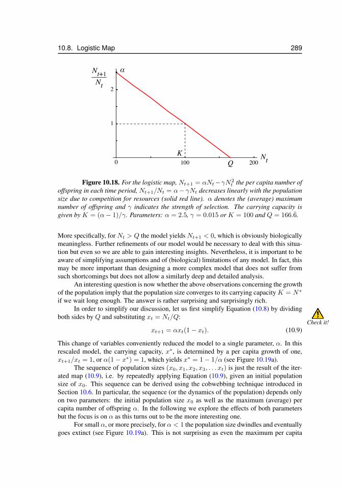
10.8. Logistic Map 289
100 200
1
2
Nt
Nt+1Nt
K0 Q
α
Figure 10.18. For the logistic map, Nt+1 = αNt−γN2t the per capita number of
offspring in each time period, Nt+1/Nt = α− γNt decreases linearly with the populationsize due to competition for resources (solid red line). α denotes the (average) maximumnumber of offspring and γ indicates the strength of selection. The carrying capacity isgiven by K = (α− 1)/γ. Parameters: α = 2.5, γ = 0.015 or K = 100 and Q = 166.6.
More specifically, for Nt > Q the model yields Nt+1 < 0, which is obviously biologicallymeaningless. Further refinements of our model would be necessary to deal with this situa-tion but even so we are able to gain interesting insights. Nevertheless, it is important to beaware of simplifying assumptions and of (biological) limitations of any model. In fact, thismay be more important than designing a more complex model that does not suffer fromsuch shortcomings but does not allow a similarly deep and detailed analysis.
An interesting question is now whether the above observations concerning the growthof the population imply that the population size converges to its carrying capacityK = N∗
if we wait long enough. The answer is rather surprising and surprisingly rich.In order to simplify our discussion, let us first simplify Equation (10.8) by dividing
both sides by Q and substituting xt = Nt/Q:Check it!
xt+1 = αxt(1− xt). (10.9)
This change of variables conveniently reduced the model to a single parameter, α. In thisrescaled model, the carrying capacity, x∗, is determined by a per capita growth of one,xt+1/xt = 1, or α(1− x∗) = 1, which yields x∗ = 1− 1/α (see Figure 10.19a).
The sequence of population sizes (x0, x1, x2, x3, . . . xt) is just the result of the iter-ated map (10.9), i.e. by repeatedly applying Equation (10.9), given an initial populationsize of x0. This sequence can be derived using the cobwebbing technique introduced inSection 10.6. In particular, the sequence (or the dynamics of the population) depends onlyon two parameters: the initial population size x0 as well as the maximum (average) percapita number of offspring α. In the following we explore the effects of both parametersbut the focus is on α as this turns out to be the more interesting one.
For small α, or more precisely, for α < 1 the population size dwindles and eventuallygoes extinct (see Figure 10.19a). This is not surprising as even the maximum per capita
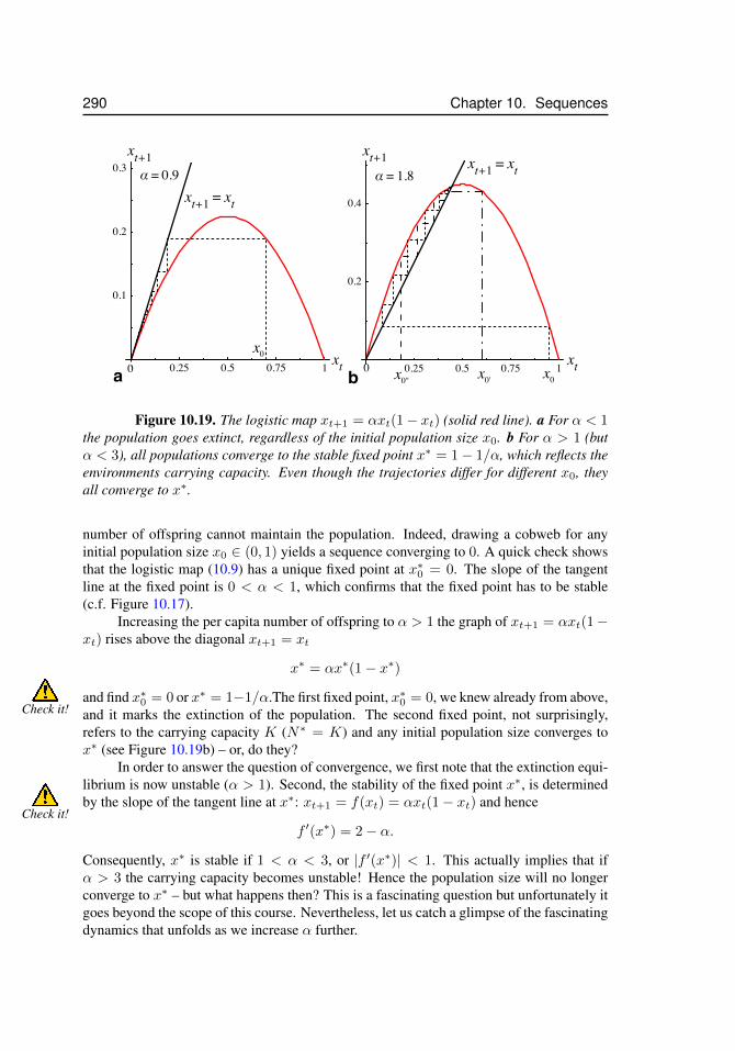
290 Chapter 10. Sequences
0.25 0.5 0.75 1
0.1
0.2
0.3
xt+1 = xt
α = 0.9
xt
xt+1
x0
0 0ba 0.25 0.5 0.75 1
0.2
0.4
xt
xt+1α = 1.8
x0x0'x0"
xt+1 = xt
Figure 10.19. The logistic map xt+1 = αxt(1− xt) (solid red line). a For α < 1the population goes extinct, regardless of the initial population size x0. b For α > 1 (butα < 3), all populations converge to the stable fixed point x∗ = 1− 1/α, which reflects theenvironments carrying capacity. Even though the trajectories differ for different x0, theyall converge to x∗.
number of offspring cannot maintain the population. Indeed, drawing a cobweb for anyinitial population size x0 ∈ (0, 1) yields a sequence converging to 0. A quick check showsthat the logistic map (10.9) has a unique fixed point at x∗0 = 0. The slope of the tangentline at the fixed point is 0 < α < 1, which confirms that the fixed point has to be stable(c.f. Figure 10.17).
Increasing the per capita number of offspring to α > 1 the graph of xt+1 = αxt(1−xt) rises above the diagonal xt+1 = xt
x∗ = αx∗(1− x∗)
and find x∗0 = 0 or x∗ = 1−1/α.The first fixed point, x∗0 = 0, we knew already from above,Check it! and it marks the extinction of the population. The second fixed point, not surprisingly,
refers to the carrying capacity K (N∗ = K) and any initial population size converges tox∗ (see Figure 10.19b) – or, do they?
In order to answer the question of convergence, we first note that the extinction equi-librium is now unstable (α > 1). Second, the stability of the fixed point x∗, is determinedby the slope of the tangent line at x∗: xt+1 = f(xt) = αxt(1− xt) and hence
Check it!f ′(x∗) = 2− α.
Consequently, x∗ is stable if 1 < α < 3, or |f ′(x∗)| < 1. This actually implies that ifα > 3 the carrying capacity becomes unstable! Hence the population size will no longerconverge to x∗ – but what happens then? This is a fascinating question but unfortunately itgoes beyond the scope of this course. Nevertheless, let us catch a glimpse of the fascinatingdynamics that unfolds as we increase α further.
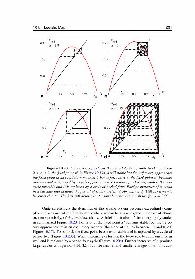
10.8. Logistic Map 291
0.25 0.5 0.75 1
0.25
0.5
0.75α = 3.1xt+1
xtx000.25 0.5 0.75 1
0.25
0.5
0.75xt+1α = 2.8
xtx00a b
c d0.25 0.5 0.75 1
0.5
1 xt+1α = 3.5
xtx0
0 0.25 0.5 0.75 1
0.5
1
α = 3.99xt+1
xtx00
Figure 10.20. Increasing α produces the period doubling route to chaos. a For2 < α < 3, the fixed point x∗ in Figure 10.19b is still stable but the trajectory approachesthe fixed point in an oscillatory manner. b For α just above 3, the fixed point x∗ becomesunstable and is replaced by a cycle of period two. c Increasing α further, renders the two-cycle unstable and it is replaced by a cycle of period four. Further increases of α resultin a cascade that doubles the period of stable cycles. d For αcritical & 3.56 the dynamicbecomes chaotic. The first 100 iterations of a sample trajectory are shown for α = 3.99.
Quite surprisingly the dynamics of this simple system becomes exceedingly com-plex and was one of the first systems where researchers investigated the onset of chaos,or, more precisely, of deterministic chaos. A brief illustration of the emerging dynamicsin summarized Figure 10.20. For α > 2, the fixed point x∗ remains stable, but the trajec-tory approaches x∗ in an oscillatory manner (the slope at x∗ lies between −1 and 0, c.f.Figure 10.17). For α > 3, the fixed point becomes unstable and is replaced by a cycle ofperiod two (Figure 10.20b). When increasing α further, the two-cycle become unstable aswell and is replaced by a period four cycle (Figure 10.20c). Further increases of α producelarger cycles with period 8, 16, 32, 64 . . . for smaller and smaller changes of α. This cas-
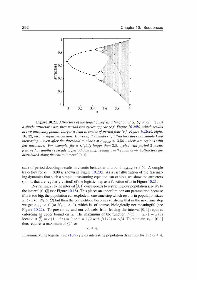
292 Chapter 10. Sequences
α
attractors
1
0.8
0.6
0.4
0.2
03 3.2 3.4 3.6 3.8 4
Figure 10.21. Attractors of the logistic map as a function of α. Up to α = 3 justa single attractor exist, then period two cycles appear (c.f. Figure 10.20b), which resultsin two attracting points. Larger α lead to cycles of period four (c.f. Figure 10.20c), eight,16, 32, etc. in rapid succession. However, the number of attractors does not simply keepincreasing – even after the threshold to chaos at αcritical ≈ 3.56 – there are regions withfew attractors. For example, for α slightly larger than 3.8, cycles with period 3 occur,followed by another cascade of period doublings. Finally, in the limit α→ 4 attractors aredistributed along the entire interval [0, 1].
cade of period doublings results in chaotic behaviour at around αcritical ≈ 3.56. A sampletrajectory for α = 3.99 is shown in Figure 10.20d. As a last illustration of the fascinat-ing dynamics that such a simple, unassuming equation can exhibit, we show the attractors(points that are regularly visited) of the logistic map as a function of α in Figure 10.21.
Restricting xt to the interval [0, 1] corresponds to restricting our population sizeNt tothe interval [0, Q] (see Figure 10.18). This places an upper limit on our parameter α becauseif α is too big, the population can explode in one time step which results in population sizesxt > 1 (or Nt > Q) but then the competition becomes so strong that in the next time stepwe get xt+1 < 0 (or Nt+1 < 0), which is, of course, biologically not meaningful (seeFigure 10.22). To prevent xt and our cobwebs from leaving the interval [0, 1] requiresenforcing an upper bound on α. The maximum of the function f(x) = αx(1 − x) islocated at df
dx = α(1 − 2x) = 0 or x = 1/2 with f(1/2) = α/4. To maintain xt ∈ [0, 1]thus requires a maximum of ≤ 1 or
α ≤ 4.
In summary, the logistic map (10.9) yields interesting population dynamics for 1 < α ≤ 4.
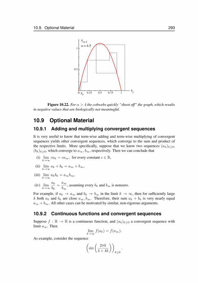
10.9. Optional Material 293
0.25 0.5 0.75 1
0.5
1
xt+1α = 4.5
xtx00
Figure 10.22. For α > 4 the cobwebs quickly “shoot off” the graph, which resultsin negative values that are biologically not meaningful.
10.9 Optional Material10.9.1 Adding and multiplying convergent sequencesIt is very useful to know that term-wise adding and term-wise multiplying of convergentsequences yields other convergent sequences, which converge to the sum and product ofthe respective limits. More specifically, suppose that we know two sequences (ak)k≥0,(bk)k≥0, which converge to a∞, b∞, respectively. Then we can conclude that
(i) limk→∞
cak = ca∞, for every constant c ∈ R,
(ii) limk→∞
ak + bk = a∞ + b∞,
(iii) limk→∞
akbk = a∞b∞,
(iv) limk→∞
akbk
=a∞b∞
, assuming every bk and b∞ is nonzero.
For example, if ak → a∞ and bk → b∞ in the limit k → ∞, then for sufficiently largek both ak and bk are close a∞, b∞. Therefore, their sum ak + bk is very nearly equala∞ + b∞. All other cases can be motivated by similar, non-rigorous arguments.
10.9.2 Continuous functions and convergent sequencesSuppose f : R → R is a continuous function, and (ak)k≥0 a convergent sequence withlimit a∞. Then
limk→∞
f(ak) = f(a∞).
As example, consider the sequence(sin
(2πk
4 + 4k
))k≥0
.
294 Chapter 10. Sequences
We have limk→∞2πk
4+4k = π2 . Since sinx is a continuous function, we know
limk→∞
sin
(2πk
4 + 4k
)= sin
(limk→∞
2πk
4 + 4k
)= sin(
π
2) = 1.
Therefore, our sequence is convergent with limk→∞ ak = 1.
10.10. Exercises 295
10.10 ExercisesExercise 10.1 Determine which of the following sequences converge or diverge
(a) {en} (b) {2−n} (c) {ne−2n} (d){
2
n
}(e)
{n2
}(f) {ln(n)}
Exercise 10.2 Does the sequence{
log
(2 + 3k + k2
3 + 2k + k2
)}k>0
converge or diverge? If it
converges, what is its limit?
Exercise 10.3 Does the sequence{
2 sin (k) cos (2k) + k2
k2 + 3k + 7
}k6−1
converge or diverge?
If it converges, what is its limit?
Exercise 10.4 Which of the following sequences are monotonic? Which are bounded?
(a){e−2k
}k>0
(b) {sin (k) cos (k)}k>0 (c) {k2}k>−3 (d){k2 + 1
k2 + 2
}k>0
Exercise 10.5 Suppose that you deposit $1000 into a bank account that earns 6% annualinterest (compounded once yearly). How long will you have to wait until the balance ofyour account reaches $2000? What is your balance after n years?
Exercise 10.6 A sequence {ak}k>0 is called arithmetic if ak+1 − ak does not depend onk; that is, ak+1 − ak is the same for each k > 0. If {ak}k>0 is an arithmetic sequencesatisfying a5 = 16 and a7 = 22, what is a30? Can you find a formula for ak?
Exercise 10.7 Imagine that two people sit down to share a pie. In the first division of thepie, a third of the pie is given to the first person and a third of what remains is given to thesecond. This process then repeats forever; in each division, the first person takes a third ofthe remaining pie and then the second person takes a third of what’s left after that. In thekth division, what fraction of the total pie does each person eat?
Exercise 10.8 Determine whether or not the following sequences converge (and the limitsif they do converge):
(a){
lnn
ln (lnn)
}n>0
(b){√
n2 + n+ 1− n}n>0
Exercise 10.9 Consider the sequence {ak}k>0 with a0 = 2 that satisfies
ak+1 =1
2(ak + 1)
for k > 0. Is this sequence bounded (from above or below)? Is it monotone?

296 Chapter 10. Sequences
Exercise 10.10 Let a > 0. Using Newton’s method, write down a sequence {xk}k>0 thatconverges to 3
√a. What are the first few terms in this sequence for a = 2?
Exercise 10.11 The Gauss map is defined by x 7→ e−αx2
+ β for some α and β. Forα = β = 1, use Newton’s method to approximate the fixed point of this map, ie. the valuex∗ such that x∗ = e−α(x∗)2 + β. How did you choose your initial point, x0?
Exercise 10.12 You are contracted to work for a week, working 8 hours a day for 5 daystotal. In the first hour of work, you earn $7. In each subsequent hour of work your hourlysalary goes up by $0.20. How much do you make in your last hour of work for the week?
Exercise 10.13 For the sequence an =n!
2n, determine lim
n→∞
anan+1
.
Exercise 10.14 For fixed a and d, consider the sequence an := a+ nd. Using
N∑n=0
n =1
2N (N + 1) ,
find a formula for∑Nn=0 an. What does the worker of Problem 10.12 earn for the week?
Exercise 10.15 Suppose that you try out a new technique to increase the amount of timeyou can spend concentrating on your homework. Before you try this new technique, youcan spend only 20 minutes working before getting distracted. After each day of using thismethod, the amount of time you can focus increases by 2%. After some amount of time,you find that you are finally able to spend one uninterrupted hour on your homework beforelooking for something else to do. Unfortunately, by this point, you’ve forgotten how longago you started using this new method. For how many days have you been using it?
Chapter 11
Series
11.1 IntroductionThis chapter builds on the concept of converging and diverging sequences developed inChapter 10 to understand when an infinite series
∑∞j=0 aj converges. Infinite series are
just sums over an infinite sequence of terms. If, for example, the sequence of terms doesnot converge, we know already that the series, or sum over this sequence, will not convergeeither. More specifically, we develop several convergence tests for infinite series. Theseconvergence tests – the so-called Divergence test, Ratio test, Series Comparison test, Inte-gral Comparison test and the optional Alternating Series test – are accompanied by severalexamples.
11.2 Infinite SeriesSeries simply represent the sum over an infinite sequence of terms. In particular, take yourfavourite infinite sequence (ak)k≥0 = (a0, a1, a2, . . .) and define a new sequence (Sn)n≥0
by setting
S0 := a0,
S1 := a0 + a1,
S2 := a0 + a1 + a2,...
Sn := a0 + a1 + a2 + · · ·+ an =
n∑j=0
aj ,...
As n → ∞ we see the term Sn as being a better and better approximation to theinfinite series
∑∞j=0 aj . Suppose that this sequence (Sn)n≥0 converges with limit S∞, i.e.
Sn → S∞. Then we interpret this limit S∞ as the sum of the infinite series∑∞j=0 aj . This
297
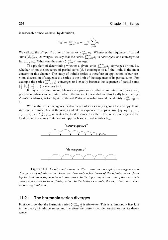
298 Chapter 11. Series
is reasonable since we have, by definition,
S∞ := limn→∞
Sn = limn→∞
n∑j=0
aj .
We call Sn the nth partial sum of the series∑∞j=0 aj . Whenever the sequence of partial
sums (Sn)n≥0 converges, we say that the series∑∞j=0 aj is convergent and converges to
limn→∞ Sn. Otherwise the series∑∞j=0 aj diverges.
The problem of determining whether a given series∑∞j=0 aj converges or not, i.e.
whether or not the sequence of partial sums (Sn) converges to a finite limit, is the mainconcern of this chapter. The study of infinite series is therefore an application of our pre-vious discussion of sequences: a series is the limit of the sequence of its partial sums. Forexample the series
∑∞j=1
12j converges to 1 exactly because the sequence of partial sums
( 12 ,
34 ,
78 ,
1516 , . . .) converges to 1.
It may at first seem incredible (or even paradoxical) that an infinite sum of non-zero,positive numbers can be finite. Indeed, the ancient Greeks did find this totally bewildering:Zeno’s paradoxes, as told by Aristotle and Plato, all revolve around the identity
∑∞j=1
12j =
1.We can think of convergence or divergence of series using a geometric analogy. If we
start on the number line at the origin and take a sequence of steps of size {a0, a1, a2, . . . ,ak, . . . }, then
∑∞k=0 ak indicates the total distance travelled. The series converges if the
total distance remains finite and we approach some fixed number S∞.
"divergence"
"convergence"
Figure 11.1. An informal schematic illustrating the concept of convergence anddivergence of infinite series. Here we show only a few terms of the infinite series: fromleft to right, each step is a term in the series. In the top example, the sum of the steps getscloser and closer to some (finite) value. In the bottom example, the steps lead to an everincreasing total sum.
11.2.1 The harmonic series divergesFirst we show that the harmonic series
∑∞n=1
1n is divergent. This is an important first fact
in the theory of infinite series and therefore we present two demonstrations of its diver-gence.
11.2. Infinite Series 299
Demonstration 1: Suppose to the contrary that∑∞n=1
1n is convergent. Then we can
rearrange the series into a sum of two convergent infinite series as shown below:
1 +1
2+
1
3+ · · · =
(1 +
1
3+
1
5+ · · ·
)+
1
2
(1 +
1
2+
1
3+ · · ·
)or, equivalently, by subtracting the second term on the right from both sides
1
2+
1
4+
1
6+ · · · = 1 +
1
3+
1
5+
1
7+ · · · .
But this this last equality is absurd because each term on the right-hand-side is strictlylarger than the corresponding term on the left-hand-side:
1/2 < 1,
1/4 < 1/3,
1/6 < 1/5, etc.
and therefore1
2+
1
4+
1
6+ · · · < 1 +
1
3+
1
5+ · · · .
Consequently, the claim that∑∞n=1
1n converges is untenable and leads to a contradiction.
Thus we conclude that the series, in fact, diverges. �
Demonstration 2: Let us consider the partial sums of the harmonic series∑∞n=1
1n
more closely. The sum of the first four terms is
1 +1
2+
1
3+
1
4> 1 +
1
2+
2
4= 1 +
1
2+
1
2.
The sum of the next four terms is
1
5+
1
6+
1
7+
1
8>
4
8=
1
2;
the sum of the next eight terms is greater than 8/16 = 1/2, and so on. Therefore the sumof the first 4 + 4 + 8 + 16 + · · ·+ 2n = 2n+1 terms of the harmonic series (i.e. S2n+1 ) isgreater than
2 +1
2+
1
2+
1
2+ · · ·+ 1
2=
1
2(n+ 3),
and, since even this lower bound grows beyond all limits for n → ∞, the harmonic seriesmust diverge, too. �
11.2.2 Geometric seriesConsider the series whose summands are obtained by repeatedly multiplying an initial terma0 by a constant factor r:
∞∑j=0
a0rj = a0(1 + r + r2 + · · · ).
300 Chapter 11. Series
For a0 = 1 we encountered this series already in chapter 1. Let us determine explicitlythe N th partial sum SN = a0(1 + r + · · · + rN ) of this series. Noting that SN − rSN =a0(1− rN+1), we find
SN = a01− rN+1
1− r.
For |r| < 1 the limit limN→∞1−rN+1
1−r exists and we have
∞∑j=0
a0rj = a0
1
1− r, whenever |r| < 1. (11.1)
The geometric series diverges whenever |r| ≥ 1 (and a0 6= 0) because the sequence(a0r
j)j≥0 does not converge to zero. In fact, for |r| > 1 and a0 > 0 we have∑Nj=0 a01j ≤∑N
j=0 a0rj , and already the left-hand-side grows without bound as N →∞.
Example: Evaluate∞∑k=2
4k−2
5k−1.
Solution:∞∑k=2
4k−2
5k−1=
1
5
∞∑k=2
4k−2
5k−2=
1
5
∞∑k=2
(4
5
)k−2
.
Reindexing the series yields
1
5
∞∑k=2
(4
5
)k−2
=1
5
∞∑k=0
(4
5
)k=
1
5
1
1− 4/5= 1.
♦Note that the restriction |r| < 1 in Equation (11.1) is important. For example, for
r = 1, Equation (11.1) yields the questionable result
∞∑j=0
1?=
1
0,
but at least we can interpret this result in the limit r → 1 and then the expression becomesmore ‘meaningful’ – both sides of the expressions diverge to∞. For r = −1 the formulayields another suspicious identity
∞∑j=0
(−1)j?=
1
2.
Of course, it is nonsensical because the series∑∞j=0(−1)j is divergent. Indeed, the se-
quence of partial sums is the divergent sequence (1, 0, 1, 0, 1, 0, . . .).
11.2. Infinite Series 301
11.2.3 Telescoping seriesCertain series have significant cancellation between successive terms. For instance oneimmediately computes
∞∑j=1
(1
k7− 1
(k + 1)7
)= 1.
Indeed, the series has the partial sums SN :
S1 =1
1− 1
27
S2 =
(1
1− 1
27
)+
(1
27− 1
37
)= 1− 1
37
S3 =
(1
1− 1
27
)+
(1
27− 1
37
)+
(1
37− 1
47
)= 1− 1
47
...
SN = 1− 1
(N + 1)7.
Therefore, limN→∞
SN = limN→∞
(1− 1
(N+1)7
)= 1.
The type of cancellation occuring in the partial sums of the series leads us to often call∞∑j=1
(1k7 −
1(k+1)7
)a telescoping series. These types of series frequently arise from partial
fraction decompositions and lead to very convenient and direct summation formulas.
Example: Consider the series
S =
∞∑k=2
1
k2 − 1.
Solution: Using the identity 1x2−1 = 1
2
(1
x−1 −1
x+1
)therefore yields
∑k≥2
1
k2 − 1=
1
2
∑k≥2
(1
k − 1− 1
k + 1
).
Note that this series is telescoping and we get
S =
(1− 1
2
)+
(1
2− 1
3
)+
(1
3− 1
4
)+
(1
4− 1
5
)+ · · · = 1.
♦
302 Chapter 11. Series
11.3 Convergence Tests for Infinite Series11.3.1 Divergence Test
If the series∑∞j=0 aj converges, then the sequence (ak)k≥0 converges to 0,
i.e. the summands ak converge to zero.
Conversely, if the summands do not converge to zero, then the series diverges. The diver-gence test is a simple way to detect the divergence of a series.
Justification: The difference between two successive partial sums is SN+1 − SN =aN+1. If the partial sums converge to ∞, i.e. SN → S∞, then necessarily the differenceSN+1 − SN must be converging to 0 and hence aN+1 → 0. �
Warning: There are many, many, many (!) divergent series∑∞j=0 aj with the
property that ak → 0. The simplest instance is the divergent harmonic series∑∞k=1
1k . The point is: knowing that a series has terms converging to zero is
not sufficient to guarantee that the series converges!
Example 1: Determine the convergence or divergence of the series
∞∑k=0
arctan(k).
Solution: Sincelimk→∞
arctan(k) =π
26= 0,
we know immediately that the series is divergent. ♦
Example 2: Does the following series converge
∞∑k=0
k√k2 + 1
?
Solution: We havelimk→∞
k√k2 + 1
= 1 6= 0,
and therefore the series is divergent. ♦
Example 3: Does the geometric series converge
∞∑k=0
(2
3
)k?
11.3. Convergence Tests for Infinite Series 303
Solution: We have
limk→∞
(2
3
)k= 0,
and hence we cannot answer the question based on the divergence test. Although, fromprevious discussions we already know that this geometric series indeed converges. ♦
11.3.2 Comparison Test
If |ak| ≤ bk and∞∑k=0
bk converges to b∞, then∞∑j=0
aj converges with limit
a∞ ≤ b∞.
Justification: The assumptions imply that the partial sums SN of the series∑∞j=0 |aj |
are increasing monotonically and bounded from above by b∞. But a bounded monotonicsequence converges. That is to say, S∞ exists and is ≤ b∞. So the series
∑∞j=0 aj con-
verges (more precisely, converges absolutely, see Section 11.5.1) with limit a∞ ≤ S∞ ≤b∞, as desired. �
For example the series∑∞n=1
1n2 converges (Euler discovered that the series con-
verges to π2
6 ). By comparison, we conclude, for example, that the series∑∞n=1
11+n2 also
converges.
Example 1: Determine whether the following series converges
∞∑k=1
1√1 + k2
.
Solution: We havelimk→∞
1√1 + k2
= 0,
so the series possibly converges. Note that k2 ≤ k2 + 1 ≤ 2k2, and therefore k ≤√1 + k2 ≤ k
√2. So we have
1√2
∞∑k=1
1
k≤∑k≥1
1√1 + k2
.
Knowing that the harmonic series∑∞k=1 k
−1 diverges, we find∞ ≤∑k≥1
1√1+k2
. Hencethe series diverges. ♦
Example 2: Determine whether the following series converges
∞∑k=1
√k√
1 + k2.
304 Chapter 11. Series
Solution: We have
limk→∞
√k√
1 + k2= 0
and hence the series may possibly converge. However, recognizing that k−1/2 ≥ k−1
whenever k ≥ 1, we get∑∞k=0 k
−1/2 ≥∑∞k=0 k
−1 but the right-hand-side is simply thediverging harmonic series and hence our series must diverge as well.
Alternatively, for large k our series is comparable to∑∞k=1
1√k
. In Chapter 7 weidentify the series
∑∞k=0 k
p as a so-called p-series, and show that for p = −1/2 it isdivergent based on the Integral Comparison test (see Section 11.4). ♦
Example 3: Determine whether the following series converges:
∞∑k=0
1
2k + 1.
Solution: Evidently limk→∞1
2k+1 = 0, so the series may possibly converge. Considerthe identity
∞∑k=1
1
k=
∞∑k=0
1
2k + 1+
∞∑k=1
1
2k,
where, of course, the series on the left-hand-side is the divergent harmonic series. There-fore we know that at least one (or possibly both) of the series
∑∞k=0
12k+1 ,
∑∞k=1
12k must
diverge. Otherwise the sum of two finite numbers would have to be infinite, which is im-possible. Note that because of
1 >1
2>
1
3>
1
4>
1
5>
1
6>
1
7>
1
8>
1
9>
1
10> · · ·
we have∞∑k=0
1
2k + 1>
∞∑k=1
1
2k>
∞∑k=1
1
2k + 1.
Therefore, the series∑∞k=0
12k+1 and
∑∞k=1
12k either both converge or both diverge. That
is, their ‘fates’ are inseparable. Since we already know that at least one of them is diver-gent, we necessarily conclude that both are divergent. In particular, the series
∑k≥0
12k+1
diverges. ♦
11.3. Convergence Tests for Infinite Series 305
11.3.3 Ratio Test
Given a series∑∞j=0 aj , set
ρ := limk→∞
∣∣∣∣ak+1
ak
∣∣∣∣ .If ρ < 1, then the series converges (absolutely, see Section 11.5.1). If ρ > 1,then the series diverges. If ρ = 1 or ρ does not exist, then the test fails:the series could converge (absolutely or conditionally, see Section 11.5.1), ordiverge.
Justification: We show that∑∞j=0 aj converges if ρ exists and ρ < 1 holds. In particu-
lar, we compare∑∞j=0 aj to the convergent geometric series
∑∞j=0 ρ
j . Because ρ exists, wehave |ak+1| ≈ ρ|ak| for sufficiently large k. Then the series
∑∞j=k |aj | ≈ |ak|
∑∞j=0 ρ
j .But ρ < 1 means
∑∞j=0 ρ
j converges. Therefore,
∞∑j=0
|aj | =k∑j=0
|aj |+∞∑
j=k+1
|aj |,
but both sums on the right are finite – the first is a finite sum and the second is convergentbecause it can be approximated by a geometric series. Hence,
∑∞j=0 |aj | converges, and
consequently∑∞j=0 aj converges. �
Example 1: Determine whether the exponential series converges:
∞∑n=1
1
n!.
Solution: This series has
ρ = limn→∞
n!
(n+ 1)!= limn→∞
1
n+ 1= 0
and hence the series converges. In Chapter 12 we will discover why this series is called theexponential series. ♦
Example 2: Consider the convergence of the p-series:∑k=1
k−p.
306 Chapter 11. Series
Solution: The ‘p’-series yields
ρ = limk→∞
(k + 1
k
)p= 1.
Therefore the ratio test is inconclusive. For p = 1, the series is the divergent harmonicseries. For p = 2, the series has the form 1 + 2−2 + 3−2 + · · · . In Chapter 7 we will showthat the series
∑∞n=1 n
−p is convergent for p > 1 and divergent otherwise using anothertest, the Integral Comparison test (see Section 11.4). ♦
Similarly, the ratio test is inconclusive for the series
∞∑k=1
1
k(k + 1)
or, more generally,∞∑k=1
1
k(k + 1) · · · (k + p)
for any integer p > 0. Again, the Integral Comparison test will reveal that these seriesconverge.
Example 3: Consider the series∑∞j=0 aj where the terms aj are defined recursively as
follows: set a0 = 1 and define
ak+1 =1 + cos(k)√
kak
for k ≥ 0. Use the ratio test to determine whether or not the series converges.
Solution: The series converges because
ρ = limk→∞
∣∣∣∣ak+1
ak
∣∣∣∣ = limk→∞
∣∣∣∣1 + cos(k)√k
∣∣∣∣ = 0 < 1.
♦
Example 4: Determine all values of λ for which the following series converges:
∞∑k=1
(λ− 1)k(k + 2)
2k(k + 3).
Solution: Appealing directly to the Ratio test we evaluate
ρ = limk→∞
∣∣∣∣∣∣(λ−1)k+1(k+3)
2k+1(k+4)
(λ−1)k(k+2)2k(k+3)
∣∣∣∣∣∣ =
∣∣∣∣λ− 1
2
∣∣∣∣ .
11.3. Convergence Tests for Infinite Series 307
Convergence is ensured if ρ < 1, i.e. for −1 < λ < 3 (or |λ− 1| < 2) and divergence forλ > 3 and λ < −1. For λ = 3 and λ = −1 the Ratio test is inconclusive. However, forλ = 3 the terms of the series are
(λ− 1)k(k + 2)
2k(k + 3)=
2k(k + 2)
2k(k + 3)=k + 2
k + 3
and evidently these summands converge to 1 as k → ∞. From the Divergence test (seeSection 11.3.1) we conclude that the series diverges for λ = 3. Similarly, for λ = −1 theterms are
(−1)kk + 2
k + 3
and hence alternate between 1 and −1 in the limit k → ∞. Again, the Divergence teststates that the series diverges. In conclusion, the series converges only for λ in the openinterval (−1, 3) and diverges for all other values, including the boundaries −1 and 3. ♦
Example 5: Determine whether the following series converges:
∞∑k=1
kk
(3k)!.
Solution: Based on the Ratio test we get
ρ = limk→∞
∣∣∣∣ (k + 1)k+1
(3k + 3)!· (3k)!
kk
∣∣∣∣= limk→∞
∣∣∣∣ (k + 1)k
kk· k + 1
(3k + 1)(3k + 2)(3k + 3)
∣∣∣∣= limk→∞
∣∣∣∣ (k + 1)k
kk
∣∣∣∣︸ ︷︷ ︸=e
· limk→∞
∣∣∣∣ k + 1
(3k + 1)(3k + 2)(3k + 3)
∣∣∣∣︸ ︷︷ ︸=0
= 0 (11.2)
Since ρ = 0 < 1, the Ratio test permits to conclude that∑∞k=1
kk
(3k)! converges. ♦
The first limit in Equation (11.2) warrants a closer look:
limk→∞
(k + 1)k
kk= limk→∞
(1 + 1
k
)k= limk→∞
ek ln(1+1/k) = e.
Note that historically this limit limk→∞(1 + 1k )k actually serves as the definition of the
constant e. For the last equality, consider the limit of the exponent and rewrite as
limk→∞
k ln(1 + 1/k) = limk→∞
ln(1 + 1/k)1k
= limm→0
ln(1 +m)
m= limm→0
11+m
1= 1
where we used de l’Hopital’s rule and a change of variables setting m = 1/k and consid-ering the limit m→ 0.
308 Chapter 11. Series
11.4 Comparing integrals and seriesThe first principle of integrals interpreted as Riemann sums is that the area under the curvecan be arbitrarily well approximated by thin rectangles. In particular, the Riemann sumdefines the integral
∫ baf(x)dx as a limit of finite sums. More specifically, for any partition
[x0, x1], [x1, x2], . . . , [xN−1, xN ] of the interval [a, b] with a = x0 < x1 < · · · < xN−1 <xN = b, we get ∫ b
a
f(x)dx ≈N∑j=1
f(xj)(xj+1 − xj).
Now consider the improper integral∫ ∞1
f(x)dx = limb→∞
∫ b
a
f(x)dx.
Taking the ‘unit’ partition [1, 2], [2, 3], . . . , [n−1, n], . . . of the interval [0,∞), the ‘infinite’Riemann sum
∞∑k=1
f(k)((k + 1)− k) =
∞∑k=1
f(k)
represents an approximation of the indefinite integral∫∞
1f(x)dx. Conversely, the im-
proper integral∫∞
1f(x)dx represents an approximation of the infinite series
∑∞k=1 ak with
ak = f(k). In this sense improper integrals are comparable to infinite series.This relation between series and improper integrals can often be exploited to deter-
mine the convergence/divergence of an integral given the convergence/divergence of theseries – or vice versa.
11.4.1 Integral Test for convergenceMore specifically, based on the above observations we find that for a monotone decreasing,positive-valued function f(x) that∫ ∞
a
f(x) dx ≤∞∑k=a
f(k),
i.e., the improper integral provides a lower bound for the infinite series (see Figure 11.2).Hence, if the integral does not exist (diverges) then the series diverges as well. Similarly,an upper bound for the series can be derived and we get
Check it! ∫ ∞a
f(x) dx ≤∞∑k=a
f(k) ≤ f(a) +
∫ ∞a
f(x) dx.
This is the gist of the integral test for convergence:
The series∞∑k=a
f(k) converges if and only if the improper integral∫ ∞a
f(x) dx converges.
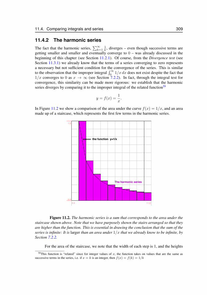
11.4. Comparing integrals and series 309
11.4.2 The harmonic seriesThe fact that the harmonic series,
∑∞k=1
1k , diverges – even though successive terms are
getting smaller and smaller and eventually converge to 0 – was already discussed in thebeginning of this chapter (see Section 11.2.1). Of course, from the Divergence test (seeSection 11.3.1) we already know that the terms of a series converging to zero representsa necessary but not sufficient condition for the convergence of the series. This is similarto the observation that the improper integral
∫∞0
1/x dx does not exist despite the fact that1/x converges to 0 as x → ∞ (see Section 7.2.2). In fact, through the integral test forconvergence, this similarity can be made more rigorous: we establish that the harmonicseries diverges by comparing it to the improper integral of the related function59
y = f(x) =1
x.
In Figure 11.2 we show a comparison of the area under the curve f(x) = 1/x, and an areamade up of a staircase, which represents the first few terms in the harmonic series.
The harmonic series
<==== the function y=1/x
0.0 11.00.0
1.0
Figure 11.2. The harmonic series is a sum that corresponds to the area under thestaircase shown above. Note that we have purposely shown the stairs arranged so that theyare higher than the function. This is essential in drawing the conclusion that the sum of theseries is infinite: It is larger than an area under 1/x that we already know to be infinite, bySection 7.2.2.
For the area of the staircase, we note that the width of each step is 1, and the heights
59This function is “related” since for integer values of x, the function takes on values that are the same assuccessive terms in the series, i.e. if x = k is an integer, then f(x) = f(k) = 1/k
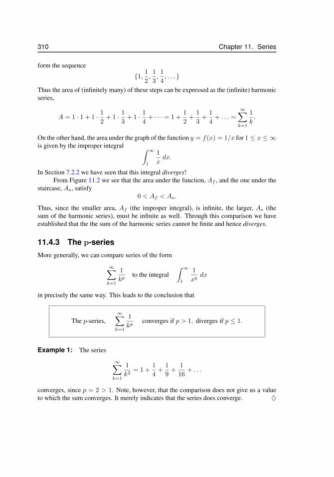
310 Chapter 11. Series
form the sequence
{1, 1
2,
1
3,
1
4, . . . }
Thus the area of (infinitely many) of these steps can be expressed as the (infinite) harmonicseries,
A = 1 · 1 + 1 · 1
2+ 1 · 1
3+ 1 · 1
4+ · · · = 1 +
1
2+
1
3+
1
4+ . . . =
∞∑k=1
1
k.
On the other hand, the area under the graph of the function y = f(x) = 1/x for 1 ≤ x ≤ ∞is given by the improper integral ∫ ∞
1
1
xdx.
In Section 7.2.2 we have seen that this integral diverges!From Figure 11.2 we see that the area under the function, Af , and the one under the
staircase, As, satisfy0 < Af < As.
Thus, since the smaller area, Af (the improper integral), is infinite, the larger, As (thesum of the harmonic series), must be infinite as well. Through this comparison we haveestablished that the the sum of the harmonic series cannot be finite and hence diverges.
11.4.3 The p-seriesMore generally, we can compare series of the form
∞∑k=1
1
kpto the integral
∫ ∞1
1
xpdx
in precisely the same way. This leads to the conclusion that
The p-series,∞∑k=1
1
kpconverges if p > 1, diverges if p ≤ 1.
Example 1: The series
∞∑k=1
1
k2= 1 +
1
4+
1
9+
1
16+ . . .
converges, since p = 2 > 1. Note, however, that the comparison does not give us a valueto which the sum converges. It merely indicates that the series does converge. ♦
11.4. Comparing integrals and series 311
Example 2: Even though the relation between series and improper integrals only indi-cates convergence/divergence of one or the other, we can exploit this relation to determineupper and lower bounds for one or the other, in case they do converge. For example, forthe above convergent series we have
S =
∞∑k=1
1
k2= 1 +
∞∑k=2
1
k2.
Interpreting the series∑∞k=2 1/k2 as a Riemann sum, we find that it approximates the
improper integral∫∞
11/x2. More precisely, if the Riemann sum uses the right endpoints
of the subintervals to approximate the area under the curve 1/x2, then
∞∑k=2
1
k2<
∫ ∞1
1
x2dx
must hold. The improper integral easily evaluates to 1. Hence the integral provides anupper bound for S and we find that S < 2 must hold. Similarly,
∞∑k=2
1
k2>
∫ ∞1
1
(x+ 1)2dx =
∫ ∞2
1
x2dx,
again assuming that the Riemann sum uses the right endpoints of the subintervals to ap-proximate the area. This time the improper integral evaluates to 1/2, which provides alower bound for the limit of the series and hence S > 3/2. Using improper integrals wecan determine upper and lower bounds for the limit of the series
∑∞k=2 1/k2 and find that
3/2 < S < 2 must hold. Indeed, the series actually converges to S = π2/6 ≈ 1.645. ♦
11.4.4 The series∞∑
n=2
1
n(lnn)α
As a last example, let us consider the function
f(x) =1
x(lnx)α,
where lnx denotes the natural logarithm (base e) and α > 0. For α 6= 1 we have by thefundamental theorem of calculus∫ b
2
dx
x(lnx)α= − 1
α− 1
[(ln b)1−α − (ln 2)1−α] .
Now we have limb→∞(ln b)1−α = 0 if α > 1 and the limit is divergent otherwise (i.e. forα < 1). In the particular case α = 1 we see that
1
x lnx=
d
dxln lnx
312 Chapter 11. Series
(recall that ddx ln f = f ′
f ) and thus by the fundamental theorem of calculus∫ b
2
dx
x lnx= ln ln b− ln ln 2.
So evidently
limb→∞
∫ b
2
dx
x lnx=∞.
Finally, by comparison, we see that the series∞∑n=2
1
n(lnn)α=
1
2(ln 2)α+
1
3(ln 3)α+ · · ·+ 1
n(lnn)α+ · · ·
converges if α > 1 and diverges if α < 1.
11.5 Optional Material11.5.1 Absolute and Conditional ConvergenceSuppose (ak)k≥0 is an arbitrary sequence of possibly both negative and positive real num-bers, for example,
(cos(n2 + 1))n≥0
or((−1)bπncn−2)n≥0.
Note that bxc is also called the floor-function and denotes the largest integer smaller orequal to x. For every sequence we can define another sequence (|ak|)k≥0, and the twocorresponding series
∞∑j=0
aj ,
∞∑j=0
|aj |.
Obviously, we have
|∞∑j=0
aj | ≤∞∑j=0
|aj |.
Therefore, if the series∑∞j=0 |aj | converges with limit a∞, then
∑∞j=0 aj converges with a
limit a∞, which must satisfy |a∞| ≤ a∞. We call a series∑∞j=0 aj conditionally conver-
gent (or, converges conditionally) if∑∞j=0 aj converges but
∑j≥0 |aj | diverges; a series∑∞
j=0 aj is absolutely convergent (or, converges absolutely) if the sum of the absolute val-ues,
∑∞j=0 |aj |, converges.
The basic example of a conditionally convergent sequence is∑∞n=1
(−1)n
n and theconvergence will be shown as an example of the Alternating Series test (see Section 11.5.3).On the other hand the harmonic series
∑∞n=1
1n is one of our favourite divergent series.
Examples of absolutely converging series are∞∑k=0
(−1)k
k!
11.5. Optional Material 313
or the geometric series∞∑j=0
(−1
2013
)j.
A rearrangement of the series∑∞j=0 aj is another series, which has exactly the same
terms, but not necessarily in the same order. That is, we rearrange the order in whichthe elements of the sequence (ak)k≥0 occur and thus rearrange the order of summation.Summing over a finite set of numbers, rearrangements yield the same sum. To be fancy,this is called the commutativity property of real numbers, i.e. 1+3+5+7 = 1+5+3+7 =7 + 1 + 5 + 3. It is, perhaps, a surprising fact that this no longer holds for infinite series.To be precise, if the series
∑∞j=0 aj converges absolutely then all rearrangements have
the same sum. However, if the series∑∞j=0 aj converges only conditionally then the sum
can change dramatically as the following example demonstrates. This behaviour was quitepuzzling to early mathematicians and philosophers studying calculus.
Example: Rearranging a conditionally convergent sequence
As an example60 the series
1
2− 1
2+
1
2− 1
2+
1
3− 1
3+
1
3− 1
3+
1
3− 1
3+
1
4− 1
4+
1
4− 1
4+
1
4− 1
4+
1
4− 1
4+
1
4− 1
4+ · · ·
has partial sums
1
2, 0,
1
2, 0,
1
3, 0,
1
3, 0,
1
3, 0,
1
4, 0,
1
4, 0,
1
4, 0,
1
4, 0, . . .
converging to 0. However the rearrangement
1
2+
1
2− 1
2− 1
2+
1
3+
1
3− 1
3− 1
3+
1
3+
1
3− 1
4− 1
4+
1
4+
1
4− 1
4− 1
4+
1
4+
1
4− 1
4− 1
4+ · · ·
has partial sums
1
2, 1,
1
2, 0,
1
3,
2
3, 1,
2
3,
1
3, 0,
1
4,
1
2,
3
4, 1,
3
4,
1
2,
1
4, 0, . . .
which diverges since they oscillate between 0 and 1. Therefore, rearrangements of the firstseries (which was converging to 0) may yield a divergent series. ♦
Given a conditionally convergent series (ak)k≥0, one might ask ‘What limits can weget from rearranging the series?’ The surprising fact is that we can get all limits! This is thecontent of the following famous theorem in the folklore of mathematics (without proof):
Theorem 11.1 (Riemann’s Rearrangement Theorem). Suppose that the series∑∞j=0 aj
converges conditionally. Then its terms can be rearranged to converge to any given limit.60Taken from Frank Morgan’s AMS textbook Real Analysis, 2005.
314 Chapter 11. Series
11.5.2 Adding and multiplying seriesArithmetic operations on infinite series only make sense if the series are convergent. When-ever this is true, then (and only then) it is true that we can exchange the order of operations.Here we write
∑k ak for an infinite series with index variable k and an unspecified lower
boundary. If two series converge absolutely,∑k ak = S and
∑k bk = T , then
(i)∑k
cak = c∑k
ak = cS, for any constant c ∈ R,
(ii)∑k
(ak + bk) =∑k
ak +∑k
bk = S + T ,
(iii) the product
(∑k
ak
)·
∑j
bj
=∑k
∑j
akbj = S · T .
Example:∞∑k=0
∞∑j=0
1
2k1
3j=
∞∑k=0
1
2k·∞∑j=0
1
3j=
(1 +
1
2+
1
4+ . . .
)(1 +
1
3+
1
9+ . . .
)=
1
1− 12
· 1
1− 13
= 2 · 3
2= 3.
11.5.3 Alternating Series Test
If the terms of a series∑∞j=0 aj alternate in sign and |ak| decreases monoton-
ically with limit zero,
|a0| ≥ |a1| ≥ |a2| . . . |ak| ≥ |ak+1| . . .→ 0,
then the series∑∞j=0 aj converges.
Justification: The partial sums SN of an alternating series∑∞k=0(−1)kak, where ak >
0, have the property that
S1 < S3 < · · · < Sodd < · · · < Seven < · · · < S2 < S0.
The odd partial sums form a bounded, monotonically increasing sequence and the evenpartial sums form a bounded, monotonically decreasing sequence. Hence, the sequences ofodd and even partial sums (S2k+1)k≥0 and (S2k)k≥0 are convergent, with limits Sodd
∞ andSeven∞ . This yields
S1 < S3 < · · · < Sodd∞ ≤ Seven
∞ < · · · < S2 < S0.
The difference between these two limits |Sodd∞ −Seven
∞ |must be less than the limit limk→∞ |S2k+1−S2k|. However, this limit goes to 0 because ak → 0. Therefore, |Sodd
∞ −Seven∞ | = 0. Finally,
since the odd and even limits are equal, the series converges. �
11.5. Optional Material 315
Example 1: The alternating series
(i)∞∑k=1
(−1)k+1 1
k
(ii)∞∑k=1
(−1)k√k
(iii)∞∑k=1
(−1)k√k +√a
(iv)∞∑k=1
(−1)k
(√k +√a)2
with a > 0 all pass the Alternating Series test and are hence conditionally convergent, i.e.the sum over the corresponding absolute values diverges. ♦
Example 2: Determine for which p the ‘translated’ alternating harmonic series con-verges:
∞∑k=1
(−1)k
k − p.
Solution: We omit the values p = 1, 2, 3, . . . because for k = p the summand is unde-fined. For p 6= 1, 2, 3, . . ., let p = dpe be the smallest integer larger than p and p = bpc bethe largest integer smaller than p. Therefore, the series
∞∑k=1
(−1)k
k − p=
p∑k=1
(−1)k
k − p+
∞∑k=p
(−1)k
k − p
converges because the first sum on the right is finite and the second sum satisfies AlternatingSeries test and consequently converges. ♦
316 Chapter 11. Series
11.6 ExercisesExercise 11.1 Which of the following series converge and which diverge? Give a reason.
(a)∞∑n=0
1−n (b)∞∑n=0
3−n (c)∞∑n=1
3
n
(d)∞∑n=0
0.1n (e)∞∑n=0
0.1−n (f)∞∑n=1
(3
n
)2
Exercise 11.2 Using the spreadsheet or a hand-drawn sketch, compare the areas repre-sented by the following integral and series.∫ ∞
1
1
x2dx,
∞∑k=1
1
k2.
Draw a sketch such that the convergence of the integral implies convergence of the series.(Hint: what kind of comparison should be set up? This will determine how you sketch thebar graph representing the series alongside the function y = f(x) = 1/x2.)
Exercise 11.3 Use the spreadsheet to show the first 100 terms in the alternating harmonicseries,
S =
100∑k=1
(−1)k+1 1
k= 1− 1
2+
1
3− 1
4+ . . . .
(You can use a bar graph to represent these terms.) On the same graph, show the first 100“partial sums”, i.e. the graph of
Sn =
n∑k=1
(−1)k+1 1
k.
To what value does this alternating harmonic series converge?
Exercise 11.4 Use the spreadsheet to show the first 100 terms in the series,
S =
100∑k=1
(−1)k+1 1
2k − 1= 1− 1
3+
1
5− 1
7+ . . . .
(You can use a bar graph to represent these terms.) On the same graph, show the first 100“partial sums” multiplied by 4, i.e. the graph of
4SN = 4
(N∑k=1
(−1)k+1 1
2k − 1
).
Show that this converges to π. Find how many correct decimal places are achieved byadding up the first one-thousand terms of this series.
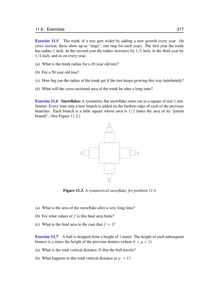
11.6. Exercises 317
Exercise 11.5 The trunk of a tree gets wider by adding a new growth every year. (Incross section, these show up as “rings”, one ring for each year). The first year the trunkhas radius 1 inch. In the second year the radius increases by 1/2 inch, in the third year by1/4 inch, and so on every year.
(a) What is the trunk radius for a 20 year old tree?
(b) For a 50 year old tree?
(c) How big can the radius of the trunk get if the tree keeps growing this way indefinitely?
(d) What will the cross-sectional area of the trunk be after a long time?
Exercise 11.6 Snowflakes A symmetric flat snowflake starts out as a square of size 1 mil-limeter. Every time step a new branch is added on the furthest edge of each of the previousbranches. Each branch is a little square whose area is 1/f times the area of its “parentbranch”. (See Figure 11.3.)
Figure 11.3. A symmetrical snowflake, for problem 11.6
(a) What is the area of the snowflake after a very long time?
(b) For what values of f is this final area finite?
(c) What is the final area in the case that f = 4?
Exercise 11.7 A ball is dropped from a height of 1 meter. The height of each subsequentbounce is p times the height of the previous bounce (where 0 < p < 1).
(a) What is the total vertical distance D that the ball travels?
(b) What happens to this total vertical distance as p→ 1?
318 Chapter 11. Series
(c) The time it takes to complete one bounce of height h is k√h where k > 0 is a constant.
What is the total time taken for the ball to travel the distance you found in part (a)?
Exercise 11.8 Does∞∑n=1
1
n2 + 5n+ 6converge? If so, find its value.
Exercise 11.9 Suppose that you wish to set up an annuity that will pay you $1,000 peryear, starting one year from now, and will continue forever. If the annual interest rate is 5%(compounded once yearly), how much will it cost you to set up this annuity?
Exercise 11.10 Does∞∑n=0
n
2n2 converge or diverge? Why?
Exercise 11.11 The integral test can also be used in reverse to establish the convergenceor divergence of improper integrals (Chapter 7). Use the integral test to determine whetheror not ∫ ∞
0
2−x2
dx
converges.
Exercise 11.12 Four people sit down to share a single pizza. The first person takes 1/2 ofthe pizza, the second takes 1/2 of what remains, the third person takes 1/2 of what remainsafter the second person, and so on. The four people continue to alternate turns taking 1/2of what remains until there is no pizza left. How much of the pizza does each person eat?
Exercise 11.13 Find integers a and b such that a/b = 0.076923, where the bar indicatesthat the sequence of numbers beneath it repeats, ie. 0.076923 = 0.076923076923076923 . . . .
Exercise 11.14 The series∑∞n=1 (−1)
n+1 1n converges by the alternating series test.
Using the fact that
∞∑n=0
rn =1
1− r
for |r| < 1, find the value of∑∞n=1 (−1)
n 1n . (Hint: integration may help.)
Exercise 11.15 Leibniz gave the following formula for calculating π:
π
4= 1− 1
3+
1
5− 1
7+ · · · =
∞∑n=0
(−1)n
(1
2n+ 1
).
Find an integer N such that the partial sum, SN =∑Nn=0 (−1)
n(
12n+1
), agrees with π/4

11.6. Exercises 319
to the first three digits beyond the decimal point. That is, find N such that∣∣∣∣∣π4 −N∑n=0
(−1)n
(1
2n+ 1
)∣∣∣∣∣ < 10−3.
(The value you find does not need to be the smallest such N , but you do need to justifywhy your answer works.)
Exercise 11.16 Consider the sequence {ak}k>0 defined by a0 = 2 and
ak+1 = ak +1
2k+1+
1
3k+1
for k > 0. Does this sequence converge? If so, what is its limit?

320 Chapter 11. Series
Chapter 12
Taylor series
12.1 IntroductionThe topic of this chapter is find approximations of functions in terms of power series,also called Taylor series. Such series can be described informally as infinite polynomials(i.e. polynomials containing infinitely many terms). Understanding when these objects aremeaningful is also related to the issue of convergence, so our discussions will rely on thebackground assembled in the previous chapters.
The theme of approximation has appeared often in our calculus course. In a previoussemester, we discussed a linear approximation to a function. The idea was to approximatethe value of the function close to a point on its graph using a straight line (the tangent line).We noted in doing so that the approximation was good only close to the point of tangency.In general, further away, the graph of the functions curves away from that straight line.This leads naturally to the question: can we improve this approximation if we include otherterms to describe this “curving away”? Here we extend such linear approximation methods.Our goal is to increase the accuracy of the linear approximation by including higher orderterms (quadratic, cubic, etc), i.e. to find a polynomial that approximates the given function(see Figure 12.1). This idea forms an important goal in this chapter.
12.2 From geometric series to Taylor polynomialsIn studying calculus, we explored a variety of functions. Among the most basic are poly-nomials, i.e. functions such as
p(x) = x5 + 2x2 + 3x+ 2.
Our introduction to differential calculus started with such functions for a reason: thesefunctions are convenient and simple to handle. We found long ago that it is easy to computederivatives of polynomials. The same can be said for integrals. One of our first examples,in Section 3.6.1 was the integral of a polynomial. We needed only use a power rule tointegrate each term. An additional convenience of polynomials is that “evaluating” thefunction, (i.e. plugging in an x value and determining the corresponding y value) can be
321
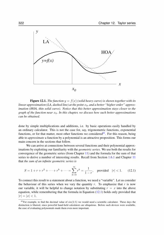
322 Chapter 12. Taylor series
HOA
x
y
y=f(x)
x0
LA
Figure 12.1. The function y = f(x) (solid heavy curve) is shown together with itslinear approximation (LA, dashed line) at the point x0, and a better “higher order” approx-imation (HOA, thin solid curve). Notice that this better approximation stays closer to thegraph of the function near x0. In this chapter, we discuss how such better approximationscan be obtained.
done by simple multiplications and additions, i.e. by basic operations easily handled byan ordinary calculator. This is not the case for, say, trigonometric functions, exponentialfunctions, or for that matter, most other functions we considered61. For this reason, beingable to approximate a function by a polynomial is an attractive proposition. This forms ourmain concern in the sections that follow.
We can arrive at connections between several functions and their polynomial approx-imations by exploiting our familiarity with the geometric series. We use both the results forconvergence of the geometric series (from Chapter 11) and the formula for the sum of thatseries to derive a number of interesting results. Recall from Section 1.6.1 and Chapter 11that the sum of an infinite geometric series is
S = 1 + r + r2 + · · ·+ rk + · · · =∞∑k=0
rk =1
1− r, provided |r| < 1. (12.1)
To connect this result to a statement about a function, we need a “variable”. Let us considerthe behaviour of this series when we vary the quantity r. To emphasize that r is nowour variable, it will be helpful to change notation by substituting r = x into the aboveequation, while remembering that the formula in Equation (12.1) holds only provided that|r| = |x| < 1.
61For example, to find the decimal value of sin(2.5) we would need a scientific calculator. These days thedistinction is blurred, since powerful hand-held calculators are ubiquitous. Before such devices were available,the ease of evaluating polynomials made them even more important.
12.2. From geometric series to Taylor polynomials 323
12.2.1 A simple expansionSubstitute the variable x = r into the series (12.1). Then formally, rewriting the above withthis substitution, leads to the conclusion that
1
1− x= 1 + x+ x2 + . . . (12.2)
We can think of this result as follows: Let
f(x) =1
1− x(12.3)
Then for −1 < x < 1, it is true that f(x) can be approximated in terms of the polynomial
p(x) = 1 + x+ x2 + . . . (12.4)
In other words, by Equation (12.1), the two expressions “are the same” for |x| < 1, in thesense that the polynomial converges to the value of the function.
We refer to this p(x) as an (infinite) Taylor polynomial62 or simply a Taylor seriesfor the function f(x). The usefulness of this kind of result can be illustrated by a simpleexample.
Example: Compute the value of the function f(x) = 1/(1 − x) for x = 0.1 withoutusing a calculator.
Solution: Plugging in the value x = 0.1 into the function directly leads to 1/(1−0.1) =1/0.9, whose evaluation with no calculator requires long division.63 Using the polynomialrepresentation, we have a simpler method:
p(0.1) = 1 + 0.1 + 0.12 + · · · = 1 + 0.1 + 0.01 + · · · = 1.11 . . .
♦
We provide a few other examples based on substitutions of various sorts using the geometricseries as a starting point.
12.2.2 A simple substitutionWe make the substitution r = −t, then |r| < 1 means that | − t| = |t| < 1, so that theformula (12.1) for the sum of a geometric series implies that:
1
1− (−t)= 1 + (−t) + (−t)2 + (−t)3 + . . .
1
1 + t= 1− t+ t2 − t3 + t4 + . . . provided |t| < 1 (12.5)
This means that we have produced a series expansion for the function 1/(1+ t). We can gofarther with this example by a new manipulation, whereby we integrate both sides to arriveat a new function and its expansion, shown next.
62A Taylor polynomial contains finitely many terms, n, whereas a Taylor series has n→∞.63This example is slightly “trivial”, in the sense that evaluating the function itself is not very difficult. However,
in other cases, we will find that the polynomial expansion is the only way to find the desired value.
324 Chapter 12. Taylor series
12.2.3 An expansion for the logarithmWe use the result of Equation (12.5) and integrate both sides. On the left, we integratethe function f(t) = 1/(1 + t) (to arrive at a logarithm type integral) and on the right weintegrate the power terms of the expansion. We are permitted to integrate the power seriesterm by term provided that the series converges. This is an important restriction that weemphasize:
Important: Manipulation of infinite series by integration, differentiation, ad-dition, multiplication, or any other “term by term” computation makes senseonly so long as the original series converges.
Provided |t| < 1, we have that∫ x
0
1
1 + tdt =
∫ x
0
(1− t+ t2 − t3 + t4 − . . .) dt
ln(1 + x) = x− x2
2+x3
3− x4
4+ . . .
This procedure has allowed us to find a series representation for a new function, ln(1 + x).
ln(1 + x) = x− x2
2+x3
3− x4
4+ . . . =
∞∑k=1
(−1)k+1xk
k. (12.6)
The sigma notation appended on the right is a compact formula that represents the pat-tern of the terms. Recall that in Chapter 1, we have gotten thoroughly familiar with suchsummation notation.64
Example: Evaluate the logarithm ln(1 + x) for x = 0.25.An expansion for the logarithm is definitely useful, in the sense that (without a scien-
tific calculator or log-tables) it is not possible to easily calculate the value of this functionat a given point. Or, of course, if you wanted to program a scientific calculator.
For x = 0.25, we cannot find ln(1.25) using simple operations. However, the valueof the first few terms of the series are computable by simple multiplication, division, andaddition: 0.25− 0.252
2 + 0.253
3 ≈ 0.2239. A scientific calculator gives ln(1.25) ≈ 0.2231,so the approximation produced by only three terms of the series is already quite good. ♦
Example: For which x is the series for ln(1 + x) in Equation (12.6) expected to con-verge?
Retracing our steps from the beginning (see Section 12.2.2), we note that the valueof t is not permitted to leave the interval |t| < 1 so we also need |x| < 1 in the integrationstep.65 We certainly cannot expect the series for ln(1 + x) to converge when |x| > 1.
64The summation notation is not crucial and should certainly not be memorized. We are usually interested onlyin the first few terms of such a series in any approximation of practical value. More important is the procedurethat lead to the different series.
65Strictly speaking, we should have ensured that we are inside this interval of convergence before we computedthe last example.
12.2. From geometric series to Taylor polynomials 325
Indeed, for x = −1, we have ln(1 + x) = ln(0), which is undefined. Also note that forx = −1 the right hand side of (12.6) becomes
−(
1 +1
2+
1
3+
1
4+ . . .
).
This is, of course, the harmonic series (multiplied by -1). But we already know fromSection 11.4.2 that the harmonic series diverges. Thus, we must avoid x = −1, sincethe expansion will not converge there, and neither is the function defined. This exam-ple illustrates that outside the interval of convergence, the series and the function become“meaningless”. ♦
Example: An expansion for ln(2).Strictly speaking, our analysis does not predict what happens if we substitute x = 1
into the expansion of the function found in Section 12.2.3, because this value of x is outsideof the permitted range −1 < x < 1 in which the Taylor series can be guaranteed toconverge. It takes some deeper mathematics (Abel’s theorem) to prove that the result ofthis substitution actually makes sense, and converges, i.e. that
ln(2) = 1− 1
2+
1
3− 1
4+ . . .
We state without proof here that the alternating harmonic series converges to ln(2). ♦
Example: An expansion for arctan(x).Suppose we make the substitution r = −t2 into the geometric series formula, and
recall that we need |r| < 1 for convergence. Then
1
1− (−t2)= 1 + (−t2) + (−t2)2 + (−t2)3 + . . .
1
1 + t2= 1− t2 + t4 − t6 + t8 + . . . =
∞∑k=0
(−1)nt2n
This series converges provided |t| < 1. Now integrate both sides, and recall that theantiderivative of the function 1/(1 + t2) is arctan(t). Then∫ x
0
1
1 + t2dt =
∫ x
0
(1− t2 + t4 − t6 + t8 + . . .) dt
arctan(x) = x− x3
3+x5
5− x7
7+ . . . =
∞∑k=1
(−1)k+1 x(2k−1)
(2k − 1). (12.7)
♦
Example: An expansion for π.For a particular application, consider plugging in x = 1 into Equation (12.7). Then
arctan(1) = 1− 1
3+
1
5− 1
7+ . . .
326 Chapter 12. Taylor series
But arctan(1) = π/4. Thus, we have found a way of computing the irrational number π,namely
π = 4
(1− 1
3+
1
5− 1
7+ . . .
)= 4
( ∞∑k=1
(−1)k+1 1
(2k − 1)
).
While it is true that this series converges, the convergence is slow. Check this by adding upthe first 100 or 1000 terms of this series with a spreadsheet or other computer software. Thismeans that it is not practical to use such a series as an approximation for π. In particular,there are other series that converge to π very rapidly. Those are used in any practicalapplication – including software packages, where it is not enough to store the first 16 or sodigits.
12.3 Taylor Series: a systematic approachIn Section 12.2, we found a variety of Taylor series expansions directly from manipulationsof the geometric series. Here we ask how such Taylor series can be constructed moresystematically, if we are given a function that we want to approximate. 66
Suppose we have a function which we want to represent by a power series,
f(x) = a0 + a1x+ a2x2 + a3x
3 + . . . =
∞∑k=0
akxk.
Here we will use the function f(x) to directly determine the coefficients ak. To calculatea0, let x = 0 and note that
f(0) = a0 + a10 + a202 + a303 + . . . = a0.
We conclude thata0 = f(0).
By differentiating both sides we find the following:
f ′(x) = a1 + 2a2x+ 3a3x2 + . . .+ kakx
k−1 + . . .
f ′′(x) = 2a2 + 2 · 3a3x+ . . .+ (k − 1)kakxk−2 + . . .
f ′′′(x) = 2 · 3a3 + . . .+ (k − 2)(k − 1)kakxk−3 + . . .
f (k)(x) = 1 · 2 · 3 · 4 . . . kak + . . .
Here we have used the notation f (k)(x) to denote the k’th derivative of the function. Nowevaluate each of the above derivatives at x = 0. Then
f ′(0) = a1 ⇒ a1 = f ′(0)
f ′′(0) = 2a2 ⇒ a2 =f ′′(0)
2
f ′′′(0) = 2 · 3a3 ⇒ a3 =f ′′′(0)
2 · 3
f (k)(0) = k! ak ⇒ ak =f (k)(0)
k!66The development of this section was motivated by online notes by David Austin.

12.3. Taylor Series: a systematic approach 327
This gives us a recipe for calculating all coefficients ak. This means that if we can computeall the derivatives of the function f(x), then we know the coefficients of the Taylor seriesas well:
f(x) =
∞∑k=0
f (k)(0)
k!xk (12.8)
Because we have evaluated all the coefficients by the substitution x = 0, we say that theresulting power series is the Taylor series of the function centered at x = 0, which issometimes also called the Maclaurin series.
12.3.1 Taylor series for the exponential function, ex
Consider the function f(x) = ex. All the derivatives of this function are equal to ex. Inparticular,
f (k)(x) = ex ⇒ f (k)(0) = 1.
So that the coefficients of the Taylor series are
ak =f (k)(0)
k!=
1
k!.
Therefore the Taylor series for ex about x = 0 is
1 + x+x2
2+x3
6+x4
24+ . . .+
xk
k!+ . . . =
∞∑k=0
xk
k!
This is a very interesting series. We state here without proof that this series converges forall values of x. Further, the function defined by the series is in fact equal to ex that is,
ex = 1 + x+x2
2+x3
6+ . . . =
∞∑k=0
xk
k!(12.9)
The implication is that the function ex is completely determined (for all x values)by its behaviour (i.e. derivatives of all orders) at x = 0. In other words, the value of thefunction at x = 1, 000, 000 is determined by the behaviour of the function around x = 0.This means that ex is a very special function with superior “predictable features”. If afunction f(x) agrees with its Taylor polynomial on a region (−a, a), as was the case here,we say that f is analytic on this region. It is known that ex is analytic for all x.
Exercise: We can use the results of Equation (12.9) to establish the fact that the expo-nential function grows “faster” than any power function xn. That is the same as saying thatthe ratio of ex to xn (for any power n) increases with x. We leave this as an exercise forthe reader. ♦
328 Chapter 12. Taylor series
We can also easily obtain a Taylor series expansion for functions related to ex, with-out assembling the derivatives. We start with the result that
eu = 1 + u+u2
2+u3
6+ . . . =
∞∑k=0
uk
k!
Then, for example, the substitution u = x2 leads to
ex2
= 1 + x2 +(x2)2
2+
(x2)3
6+ . . . =
∞∑k=0
(x2)k
k!
12.3.2 Taylor series of sinxIn this section we derive the Taylor series for sinx. The function and its derivatives are
f(x) = sinx, f ′(x) = cosx, f ′′(x) = − sinx, f ′′′(x) = − cosx, f (4)(x) = sinx, . . .
After this, the cycle repeats, i.e. f(x) = f (4)(x), f ′(x) = f (5)(x), etc. This means that
f(0) = 0, f ′(0) = 1, f ′′(0) = 0, f ′′′(0) = −1, . . .
and so on in a cyclic fashion. In other words,
a0 = 0, a1 = 1, a2 = 0, a3 = − 1
3!, a4 = 0, a5 =
1
5!, . . .
Thus,
sinx = x− x3
3!+x5
5!− x7
7!+ . . . =
∞∑n=0
(−1)nx2n+1
(2n+ 1)!.
Note that all polynomials of the Taylor series of sinx contain only odd powers of x. Thisstems from the fact that sinx is an odd function, i.e. its graph is symmetric to rotationabout the origin, a concept we discussed in an earlier term. We state here without proofthat the function sinx is analytic, so that the expansion converges to the function for all x.
12.3.3 Taylor series of cosxThe Taylor series for cosx could be found by a similar sequence of steps. But in thiscase, this is unnecessary: We already know the expansion for sinx, so we can find theTaylor series for cosx by simple term by term differentiation. Since sinx is analytic, thisis permitted for all x. We leave it as an exercise for the reader to show that
cos(x) = 1− x2
2+x4
4!− x6
6!+ . . . =
∞∑n=0
(−1)nx2n
(2n)!.
Since cos(x) has symmetry properties of an even function, we find that its Taylor series iscomposed of even powers of x only.
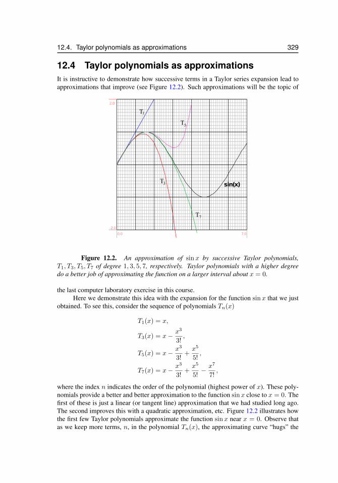
12.4. Taylor polynomials as approximations 329
12.4 Taylor polynomials as approximationsIt is instructive to demonstrate how successive terms in a Taylor series expansion lead toapproximations that improve (see Figure 12.2). Such approximations will be the topic of
sin(x)
0.0 7.0
-2.0
2.0
T1
T
T
T
5
3
7
Figure 12.2. An approximation of sinx by successive Taylor polynomials,T1, T3, T5, T7 of degree 1, 3, 5, 7, respectively. Taylor polynomials with a higher degreedo a better job of approximating the function on a larger interval about x = 0.
the last computer laboratory exercise in this course.Here we demonstrate this idea with the expansion for the function sinx that we just
obtained. To see this, consider the sequence of polynomials Tn(x)
T1(x) = x,
T3(x) = x− x3
3!,
T5(x) = x− x3
3!+x5
5!,
T7(x) = x− x3
3!+x5
5!− x7
7!,
where the index n indicates the order of the polynomial (highest power of x). These poly-nomials provide a better and better approximation to the function sinx close to x = 0. Thefirst of these is just a linear (or tangent line) approximation that we had studied long ago.The second improves this with a quadratic approximation, etc. Figure 12.2 illustrates howthe first few Taylor polynomials approximate the function sinx near x = 0. Observe thatas we keep more terms, n, in the polynomial Tn(x), the approximating curve “hugs” the
330 Chapter 12. Taylor series
graph of sinx over a longer and longer range. The student will be asked to use the spread-sheet, together with some calculations as done in this section, to produce a composite graphsimilar to Figure 12.2 for other functions.
Example: Estimating the error of approximations. For a given value of x close to thebase point (at x = 0), the error in the approximation between the polynomials and thefunction is the vertical distance between the graphs of the polynomial and the function,here again choose sinx as an illustration. For example, at x = 2 radians sin(2) = 0.9093(as found on a scientific calculator). The approximations are:
(a) T1(2) = 2, which is very inaccurate,
(b) T3(2) = 2− 23/3! ≈ 0.667 which is too small,
(c) T5(2) ≈ 0.9333 that is much closer and
(d) T7(2) ≈ .9079 that is closer still.
In general, we can approximate the size of the error using the next term that would occur inthe polynomial if we kept a higher order expansion. The details of estimating such errorsis omitted from our discussion. ♦
12.4.1 Taylor series centered at aAll Taylor series discussed so far were centered at x = 0. Now we want to extend theconcept of Taylor series to derive a polynomial representation of a function f(x) centeredat an arbitrary point x = a. The crucial idea for the derivation of the Taylor series was thatf(x) and its derivatives are subsequently evaluated at x = 0 in order to obtain polynomialsthat represent better and better approximations of f(x) in the vicinity of 0. In exactly thesame spirit we can approximate f(x) at an arbitrary point x = a:
f(x) =
∞∑k=0
f (k)(a)
k!(x− a)k. (12.10)
Alternatively, you can imagine to translate f(x) horizontally by distance a and apply theTaylor expansion centered at y = 0 for the translated function f(y) with y = x− a.
12.5 Applications of Taylor seriesIn this section we illustrate some of the applications of Taylor series to problems that maybe difficult to solve using other conventional methods. Some functions do not have anantiderivative that can be expressed in terms of other simple functions. Integrating thesefunctions can be a problem, as we cannot use the Fundamental Theorem of Calculus. How-ever, in some cases, we can approximate the value of the definite integral using a Taylorseries. Another application of Taylor series is to compute an approximate solution to dif-ferential equations.
12.5. Applications of Taylor series 331
12.5.1 Evaluate an integral using Taylor seriesEvaluate the definite integral ∫ 1
0
sin(x2) dx.
A simple substitution (e.g. u = x2) will not work here, and we cannot find an antideriva-tive. Here is how we might approach the problem using Taylor series: We know that theseries expansion for sin(t) is
sin t = t− t3
3!+t5
5!− t7
7!+ . . .
Substituting t = x2, we have
sin(x2) = x2 − x6
3!+x10
5!− x14
7!+ . . .
In spite of the fact that we cannot find an anti-derivative of the function, we can derive theanti-derivative of the Taylor series, term by term – just as we would for a long polynomial:∫ 1
0
sin(x2) dx =
∫ 1
0
(x2 − x6
3!+x10
5!− x14
7!+ . . .) dx
=
(x3
3− x7
7 · 3!+
x11
11 · 5!− x15
15 · 7!+ . . .
) ∣∣∣∣10
=1
3− 1
7 · 3!+
1
11 · 5!− 1
15 · 7!+ . . .
This is an alternating series with terms of decreasing magnitude and so we know that itconverges. After adding up the first few terms, the pattern becomes clear and with somepatience we find that the series converges to 0.310268.
12.5.2 Series solution of a differential equationWe are already familiar with the differential equation and initial condition that describesunlimited exponential growth.
dy
dx= y,
y(0) = 1.
Indeed, from previous work, we know that the solution of this differential equation andinitial condition is y(x) = ex, but we will pretend that we do not know this fact to illustratethe usefulness of Taylor series. In some cases, where separation of variables does not work,this option has great practical value.
Let us express the “unknown” solution to the differential equation as
y = a0 + a1x+ a2x2 + a3x
3 + a4x4 + . . .
332 Chapter 12. Taylor series
Our task is to determine values for the coefficients ai.Since this function satisfies the condition y(0) = 1, we must have y(0) = a0 = 1.
Differentiating this power series leads to
dy
dx= a1 + 2a2x+ 3a3x
2 + 4a4x3 + . . .
But according to the differential equation, dydx = y. Hence, the two Taylor series must
match, i.e.
a0 + a1x+ a2x2 + a3x
3 + a4x4 + . . . = a1 + 2a2x+ 3a3x
2 + 4a4x3 + . . .
In particular, this equality must hold for all values of x. However, this can only happenif the coefficients of like terms are the same, i.e. if the constant terms on either side ofthe equation are equal, if the terms of equal power of x on either side are equal. Equatingcoefficients, we obtain:
a0 = a1 = 1, ⇒ a1 = 1,
a1 = 2a2, ⇒ a2 =a1
2=
1
2,
a2 = 3a3, ⇒ a3 =a2
3=
1
2 · 3,
a3 = 4a4, ⇒ a4 =a3
4=
1
2 · 3 · 4,
an−1 = nan, ⇒ an =an−1
n=
1
1 · 2 · 3 . . . n=
1
n!. (12.11)
This means that
y = 1 + x+x2
2!+x3
3!+ . . .+
xn
n!+ . . . = ex,
which, as we have seen, is the expansion for the exponential function. This agrees withthe solution we have been expecting. In the example here shown, we would hardly needto use series to arrive at the right conclusion. However, another example is discussed inthe optional material, Section 12.7.1, where we would not find it as easy to discover thesolution by other techniques discussed previously.
12.6 SummaryThe main points of this chapter can be summarized as follows:
1. We discussed Taylor series and showed that some can be found using the formulafor convergent geometric series. Two examples of Taylor series that were obtainedin this way are
ln(1 + x) = x− x2
2+x3
3− x4
4+ . . . for |x| < 1
and
arctan(x) = x− x3
3+x5
5− x7
7+ . . . for |x| < 1
12.6. Summary 333
2. For Taylor series, we considered:
(a) For what range of values of x can we expect the series to converges?
(b) Suppose we approximate the function on the right by a finite number of terms onthe left. How good is that approximation?
(c) If we include more and more such terms, does that approximation get better andbetter? (i.e., does the series converge to the function?)
(d) Is the convergence rate rapid?
Some of these questions occupy the attention of mathematicians, and are beyond thescope of an introductory calculus course.
3. More generally, we showed that the Taylor series for a function about x = 0,
f(x) = a0 + a1x+ a2x2 + a3x
3 + . . . =
∞∑k=0
akxk.
can be found by computing the coefficients
ak =f (k)(0)
k!
4. As applications we discussed Taylor series to approximate a function, to find an ap-proximation for a definite integral of a function, and to solve a differential equation.
334 Chapter 12. Taylor series
12.7 Optional Material12.7.1 Airy’s equationAiry’s equation arises in the study of optics, and (with initial conditions) is as follows:
y′′ = xy, y(0) = 1, y′(0) = 0.
This differential equation cannot be easily solved using the integration techniques discussedin this course. However, we can solve it using Taylor series. As in Section 12.5.2, we writethe solution as an arbitrary series:
y = a0 + a1x+ a2x2 + a3x
3 + a4x4 + a5x
5 + . . .
Using the information from the initial conditions, we get y(0) = a0 = 1 and y′(0) = a1 =0. Now we can write down the derivatives:
y′ = a1 + 2a2x+ 3a3x2 + 4a4x
3 + 5a5x4 + . . .
y′′ = 2a2 + 2 · 3x+ 3 · 4x2 + 4 · 5x3 + . . .
The equation then gives
y′′ = xy
2a2 + 2 · 3a3x+ 3 · 4a4x2 + 4 · 5a5x
3 + . . . = x(a0 + a1x+ a2x2 + a3x
3 + . . .)
2a2 + 2 · 3a3x+ 3 · 4a4x2 + 4 · 5a5x
3 + . . . = a0x+ a1x2 + a2x
3 + a3x4 + . . .
Again, we can equate the coefficients of x, and use a0 = 1 and a1 = 0, to obtain
2a2 = 0⇒ a2 = 0,
2 · 3a3 = a0 ⇒ a3 =1
2 · 3,
3 · 4a4 = a1 ⇒ a4 = 0,
4 · 5a5 = a2 ⇒ a5 = 0,
5 · 6a6 = a3 ⇒ a6 =1
2 · 3 · 5 · 6.
This gives us the first few terms of the solution:
y = 1 +x3
2 · 3+
x6
2 · 3 · 5 · 6+ . . .
If we continue in this way, we can determine any number of terms of the series.
12.8. Exercises 335
12.8 ExercisesExercise 12.1 The Taylor series for the function sin(x) is given by
sin(x) = x− x3
3!+x5
5!− x7
7!+ . . . .
Find the Taylor series ofy = cos(x)
by differentiating this function. Using the spreadsheet, plot the following functions (on thesame graph):
y = cos(x), y = T1(x), y = T2(x), y = T3(x), y = T4(x)
where Tk is the polynomial made up of the first k (non-zero) terms in the Taylor series forcos(x).
Exercise 12.2 An expansion for the function ex is given by
ex = 1 + x+x2
2+x3
6+ . . . =
∞∑n=0
xk
k!.
Use the first seven terms of this series to estimate the value of the base of natural logarithms,i.e. of e1.
Exercise 12.3 Find the Taylor series for each of the following functions about x = 0:
(a) f(x) = x cos(x),
(b) e−x2
(c)sin(x)
x
(d) Use your results to find a Taylor series representation for the following integrals:
(i)∫ x
0
x cos(x) dx (ii)∫ x
0
e−x2
dx
Exercise 12.4 Find the Taylor series at x = 0 of the following functions:
(a) f(x) = e−x2/2 (b) f(x) = ln(1 + x)
(c) f(x) =√x sin
√x (d) f(x) =
ex + e−x
2
Exercise 12.5 Using the Taylor series of f(x) near a point x∗, the value of a smoothfunction f(x) in the vicinity of x∗ can be approximated by f(x∗) and f (k)(x∗) (wheref (k)(x) is the kth derivative of f(x)), and the distance between x and x∗, ∆x = x− x∗:
f(x) = f(x∗)+f ′(x∗)∆x+f ′′(x∗)
2!(∆x)2 +
f ′′′(x∗)
3!(∆x)3 + · · ·+ f (k)(x∗)
k!(∆x)k+ · · ·
336 Chapter 12. Taylor series
where k! = k · (k − 1) · (k − 2) · · · 3 · 2 · 1 is called the factorial of the integer k.If |∆x| � 1 (i.e., x is very close to x∗), (∆x)k becomes negligibly small. When
keeping only the first k terms of the series, the error arising from throwing away all theterms subsequent to the kth term typically has a magnitude of the same order as |∆x|k+1.This error can be made arbitrarily small by keeping more terms in the series. Thus, Taylorseries is often used in calculating the approximate value of a function that is not a polyno-mial.
For example, knowing that√
25 = 5, we can calculate an approximate value of√
26by using the Taylor series. Note that,
√26 =
√25 + 1 =
√25(1 +
1
25) = 5
√1 +
1
25.
Now let x∗ = 1 and x = 1 + 125 , thus ∆x = x − x∗ = 1
25 = 0.04 which is small. Nowusing the Taylor series and keeping the first three terms:
√x ≈√x∗ + [(
√x)′]|x=x∗∆x+
[(√x)′′]|x=x∗
2!(∆x)2
which yields √1 +
1
25≈ 1 +
1
20.04− 1
80.042 = 1.0198.
Thus,√
26 = 5
√1 +
1
25≈ 5 · 1.0198 = 5.099.
Using a calculator, we find√
26 = 5.0990195 . . . , which is identical for the first 4 digits.Use the first 3 terms of Taylor series to estimate the values of the following functions.
Calculate by hand and compare the result with that obtained by a scientific calculator!
(a)√
110 (Hint: 110 = 100 + 10 and√
100 = 10)
(b) e0.1 (Hint: 0.1 = 0 + 0.1 and e0 = 1)(c) cos(3) (Hint: 3 = π − (π − 3) ≈ π − 0.14 and cos(π) = −1)
(d) arctan(1.1) (Hint: arctan(1) = π/4, (arctan(x))′ = 1/(1 + x2))
Exercise 12.6 Find the Taylor series at x = 0, up to and including the xn term, for thefollowing functions:
(a) f(x) = tanx, n = 3 (b) f(x) = (x+ 1)ex, n = 4
(c) f(x) = ex2−2x, n = 3 (d) f(x) = (sinx)2, n = 6
Exercise 12.7
(a) Find a Taylor series for the function f(x) = 1/(1 + x3) about x = 0. Show that thiscan be done by making the substitution r = −x3 into the sum of a geometric series(S =
∑rk = 1
1−r ).
12.8. Exercises 337
(b) Use the same idea to find the Taylor series for the function f(t) =1
1 + t2.
(c) Use your result in part (b) to find a Taylor series for the function arctan(x). (Hint:
recall that arctan(x) =
∫ x
0
1
1 + t2dt).
Exercise 12.8 Let E(x) be the function defined by
E(x) =
∫ x
0
e−t − 1
tdt.
(a) Use the Taylor series about t = 0 for the function e−t to write down the analogousTaylor series about t = 0 for the function e−t−1
t .
(b) Use your result in part (a) to determine the Taylor series about x = 0 for the integralE(x).
Exercise 12.9 Growth of the exponential function Consider the exponential functiony = f(x) = ex. Write down a Taylor Series series expansion for this function. Divide bothsides by xn. Now examine the terms for the quantity ex/xn. Use this expansion to arguethat the exponential function grows faster than any power function.
Exercise 12.10 Find a Taylor series about x = 0 for
F (x) =
∫ x
0
ln(1 + t2) dt.
Exercise 12.11 Use a Taylor series representation to find the function y(t) that satisfiesthe differential equation y′(t) = y + b t with the initial condition y(0) = 1. This type ofequation is called a non-homogeneous differential equation. Show that when b = 0 youranswer agrees with the known exponential solution of the equation y′(t) = y.
Exercise 12.12 Use Taylor series to find the function that satisfies the following secondorder differential equation and initial conditions:
d2y
dt2+ y = 0, y(0) = 0, y′(0) = 1.
A second order differential equation is one in which a second derivative appears. Noticethat this type of differential equation comes with two initial conditions. Your answer shoulddisplay y(t) as a Taylor series expansion of the desired function. (You may be able to thenguess what elementary function has this expansion as its Taylor series.)

338 Chapter 12. Taylor series
Chapter 13
Solutions
13.1 Areas, volumes and simple sumsSolution to 1.1
(a) a5 = 4 (b) 11terms (c) 1 + 2 + 22 + 23 + 24
(d) 1 + 2 + 22 + 23 + 24 (e)3∑
n=0
3n
Solution to 1.2
(a)∞∑n=1
2n (b)∞∑n=1
1
n
(c) 1 + 3 + 9 + 27 + 81 + 243 + . . . (d) 1 +1
22+
1
33+
1
44+ . . .
(e)∞∑k=2
(1
2
)k(f)
9∑x=0
3x
(g)100∑n=0
(n+ n2) (h)100∑y=0
(y + 1)2
Solution to 1.3
(a) each sum represents 1 + 22 + 32 + 42 + 52 + ...+ 112
(b) each sum represents 0 + 1 + 4 + 9
Solution to 1.4
(a) 290 (b) 300 (c) 240 (d) 1275 (e) 1830
(f) 1785 (g) 4860 (h) 16575 (i) 5740 (j) 1650
(k) 2925 (l) 120300 (m) 3825 (n) 40425 (o) 40411
(p) 42075 (q) 18496
339
340 Chapter 13. Solutions
Solution to 1.5
(a) 2550 (b) 2500 (c) 44200 (d) 41650
Solution to 1.6 S = 7618
Solution to 1.7 The clock chimes 324 times.
Solution to 1.8 The total enclosed volume is 14400 cubic inches.
Solution to 1.9 12 frames can be made enclosing a total of 9200 cm2
Solution to 1.10
(a) 39601 (b) 1 (c) 2, 686, 700
Solution to 1.11
(a)k(k + 1)
2(b) 10, 20, 35 (c)
N(N + 1)(N + 2)
6(d) 171700
Solution to 1.12
(1) (a) The radius of the smallest disk is r1 =r
N.
(b) The radius of the k-th disk is rk =kr
N.
(2) V = π
N∑k=1
(kr
N
)2h
N= πr2h
2N2 + 3N + 1
6N2.
(3) The volume converges to V → 1
3πr2h.
Solution to 1.13
(a) k (b) 2047 (c) 2
(1− 1
211
)
Solution to 1.14
(a) Approximately 18.531, 64.002, 181.943, 487.852, and 1281.299, respectively.
(b) Approximately 6.862, 8.906, 9.618, 9.867, and 9.954, respectively.
(c) In (a), for |r| > 1, the sums increase (rapidly) with N whereas in (b), for |r| < 1, theyincrease only very slowly.
13.2. Areas 341
(d) For N →∞, the sum converges for |r| < 1 and diverges otherwise.
Solution to 1.15 If there had been enough grain on Earth, the inventor would have received264 − 1 ≈ 1.845 1019 grains.
Solution to 1.16 The total length of segments is 2047 units.
Solution to 1.17
(a)(
4
5
)12
`0 (b)1−
(45
)13
1− 45
`0 (c) 5`0
Solution to 1.18
(a) Fn =2
r0βn(b) β < 1
Solution to 1.19
(a) 2097151 branches; volume 105.6 cm3; surface 9950.57 cm2
(b) 0.625 < β < 0.7905
Solution to 1.20
(a) A = 4.829 cm2 (b) A = 5.36 cm2
13.2 AreasSolution to 2.1
(a) 55 (b) 50.5 (c) 50
Solution to 2.2
(a)1
2(b) lim
N→∞1− 1
2+
1
2N2=
1
2
Solution to 2.3 2470 < A < 2870
Solution to 2.4
(a) 8 (b) 8.375 (c) 8.75
(d) 8.9375 (e) (d)
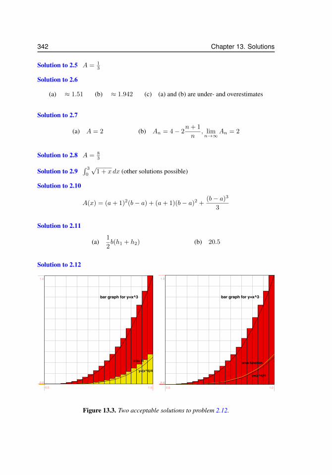
342 Chapter 13. Solutions
Solution to 2.5 A = 13
Solution to 2.6
(a) ≈ 1.51 (b) ≈ 1.942 (c) (a) and (b) are under- and overestimates
Solution to 2.7
(a) A = 2 (b) An = 4− 2n+ 1
n, limn→∞
An = 2
Solution to 2.8 A = 83
Solution to 2.9∫ 3
0
√1 + x dx (other solutions possible)
Solution to 2.10
A(x) = (a+ 1)2(b− a) + (a+ 1)(b− a)2 +(b− a)3
3
Solution to 2.11
(a)1
2b(h1 + h2) (b) 20.5
Solution to 2.12
bar graph for y=x^3
y=(x^4)/4
area fn
0.0 1.00.0
1.0
bar graph for y=x^3
area function
y=(x^4)/4
0.0 1.00.0
1.0
Figure 13.3. Two acceptable solutions to problem 2.12.

13.3. The Fundamental Theorem of Calculus 343
Solution to 2.13
(a) 1 (b) 2 (c) 2π
Solution to 2.14
(a) xk =3k
N(b)
(3
N
)4
k3 (c)34
4
(N + 1
N
)2
(d) 182.25
Solution to 2.15 A = 16.25
Solution to 2.16
(a)2w
L2(b)
HL3
6(c)
wL
3
Solution to 2.17
(a)2
3
(1−
(2
3
) 12
)(b)
1
6
13.3 The Fundamental Theorem of CalculusSolution to 3.1
(a) The Fundamental Theorem of Calculus states that if F (x) is any anti-derivative of f(x)
then∫ baf(x)dx = F (b)− F (a)
(b) the Fundamental Theorem of Calculus provides a shortcut for calculating integrals.Without it, we would have to use tedious summation and limits to compute areas,volumes, etc. of irregular regions.
Solution to 3.2 e− 1
Solution to 3.3
(a) 1 (b) 2
Solution to 3.4
(a) 2 (b) 2−√
2 (c) 1 (d) 2√
2 (e)1
2
(f) − 2 (g)8
3(h)
124
3(i)
16
3(j) 2
(k)23
3(l) 3 ln 2 (m) 2 ln(3) (n) 2(e− 1) (o)
3
4
(3 · 31/3 − 2 · 21/3
)(q) DNE (q) DNE (r) 2 (s) DNE (t) DNE
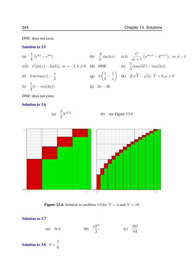
344 Chapter 13. Solutions
DNE: does not exist.
Solution to 3.5
(a)1
k
(ekx − eka
)(b)
A
ksin(kx) (c1)
C
m+ 1
(xm+1 − bm+1
), m 6= −1
(c2) C(ln(x)− ln(b)), m = −1, b 6= 0 (d) DNE (e)1
5(tan(5T )− tan(5c))
(f) 2 arctan(x)− π
2(g) 3
(1
b− 1
x
)(h) 2(
√T −√a), T > 0, a > 0
(i)1
3(1− cos(3x)) (j) 3x− 3b
DNE: does not exist.
Solution to 3.6
(a)2
3N3/2 (b) see Figure 13.4
0.0 4.00.0
2.0
0.0 16.00.0
4.0
Figure 13.4. Solution to problem 3.6 for N = 4 and N = 16.
Solution to 3.7
(a) ln 3 (b)aT 2
2(c)
255
64
Solution to 3.8 S =7
6
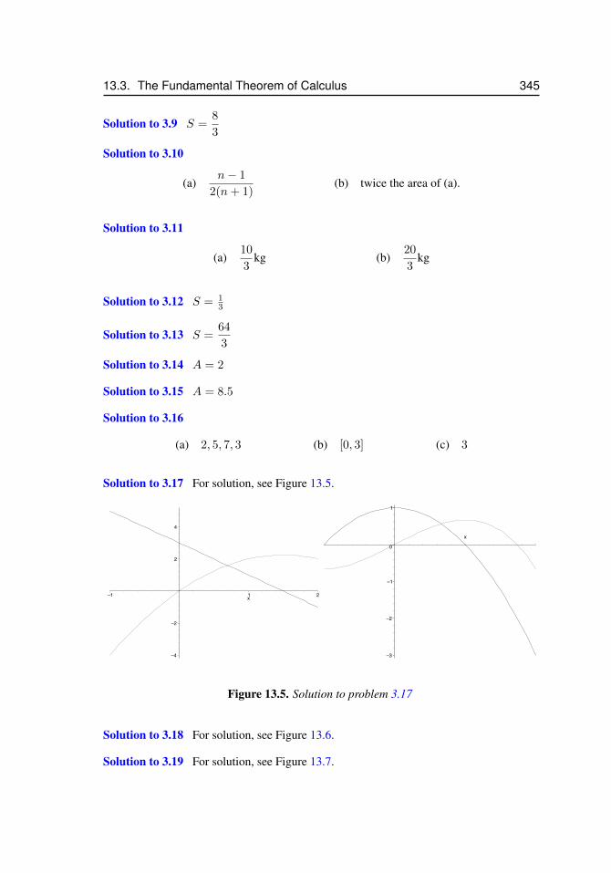
13.3. The Fundamental Theorem of Calculus 345
Solution to 3.9 S =8
3
Solution to 3.10
(a)n− 1
2(n+ 1)(b) twice the area of (a).
Solution to 3.11
(a)10
3kg (b)
20
3kg
Solution to 3.12 S = 13
Solution to 3.13 S =64
3
Solution to 3.14 A = 2
Solution to 3.15 A = 8.5
Solution to 3.16
(a) 2, 5, 7, 3 (b) [0, 3] (c) 3
Solution to 3.17 For solution, see Figure 13.5.
–4
–2
2
4
–1 1 2x
–3
–2
–1
0
1
x
Figure 13.5. Solution to problem 3.17
Solution to 3.18 For solution, see Figure 13.6.
Solution to 3.19 For solution, see Figure 13.7.
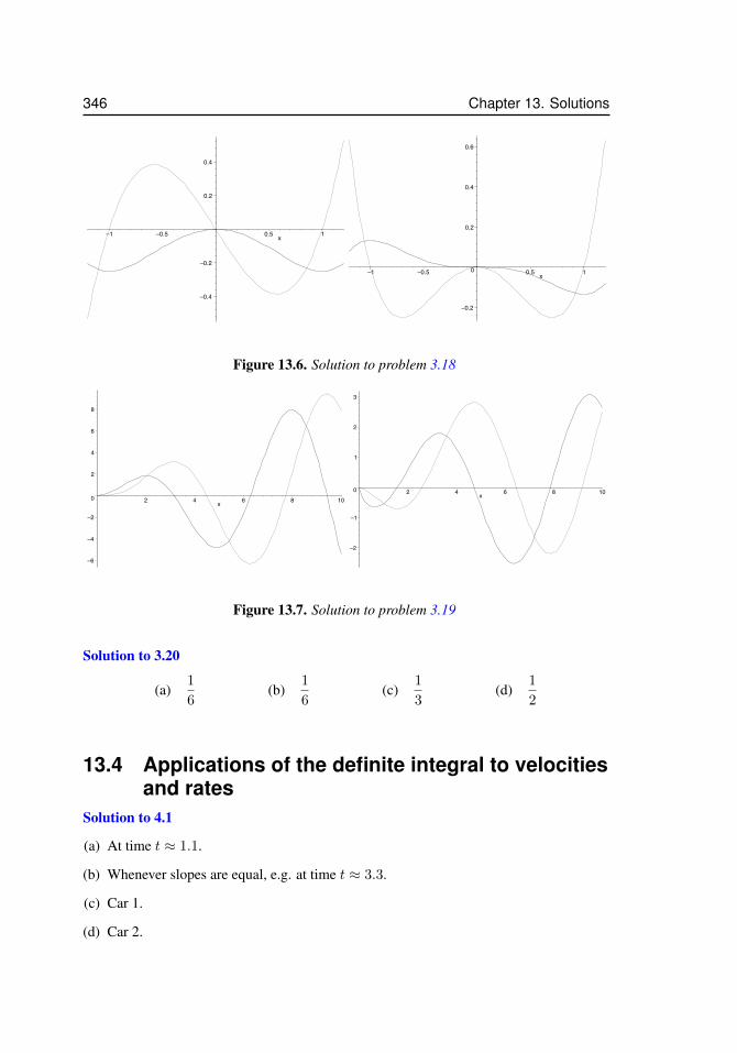
346 Chapter 13. Solutions
–0.4
–0.2
0.2
0.4
–1 –0.5 0.5 1x
–0.2
0
0.2
0.4
0.6
–1 –0.5 0.5 1x
Figure 13.6. Solution to problem 3.18
–6
–4
–2
0
2
4
6
8
2 4 6 8 10x
–2
–1
0
1
2
3
2 4 6 8 10x
Figure 13.7. Solution to problem 3.19
Solution to 3.20
(a)1
6(b)
1
6(c)
1
3(d)
1
2
13.4 Applications of the definite integral to velocitiesand rates
Solution to 4.1
(a) At time t ≈ 1.1.
(b) Whenever slopes are equal, e.g. at time t ≈ 3.3.
(c) Car 1.
(d) Car 2.
13.4. Applications of the definite integral to velocities and rates 347
(e) At time t ≈ 2.2.
Solution to 4.2
(a) a(t) = 4t+ 5 (b)19
6
Solution to 4.3
(a) k = 1 (b) 10(e−t + t− 1)
Solution to 4.4
(a) v(t) =t2
2− t3
3(b)
1
12
Solution to 4.5
(a) 231
3km (b) 32.5l
Solution to 4.6143
36
Solution to 4.7
(a)34
9s (b)
5375
81m
Solution to 4.8
(a) child2 (b) child1
Solution to 4.9 A
(23
3− 3
20cos(0.15)
)Solution to 4.10 12000$
Solution to 4.11 7.5 mg
Solution to 4.12
(a) t = 5√
2h (b)100√
2
3≈ 471.4 · 103 barrels
Solution to 4.13
(a) t = 10 h (b) t2 = 30 h (c)160
3105 gal
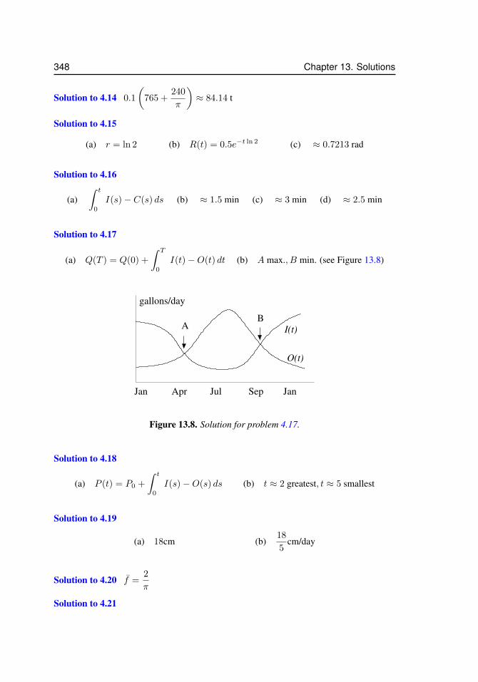
348 Chapter 13. Solutions
Solution to 4.14 0.1
(765 +
240
π
)≈ 84.14 t
Solution to 4.15
(a) r = ln 2 (b) R(t) = 0.5e−t ln 2 (c) ≈ 0.7213 rad
Solution to 4.16
(a)∫ t
0
I(s)− C(s) ds (b) ≈ 1.5 min (c) ≈ 3 min (d) ≈ 2.5 min
Solution to 4.17
(a) Q(T ) = Q(0) +
∫ T
0
I(t)−O(t) dt (b) A max., B min. (see Figure 13.8)
B
Jan Apr JanJul Sep
gallons/day
I(t)
O(t)
A
Figure 13.8. Solution for problem 4.17.
Solution to 4.18
(a) P (t) = P0 +
∫ t
0
I(s)−O(s) ds (b) t ≈ 2 greatest, t ≈ 5 smallest
Solution to 4.19
(a) 18cm (b)18
5cm/day
Solution to 4.20 f =2
π
Solution to 4.21
13.4. Applications of the definite integral to velocities and rates 349
(a) f =1
n+ 1, for n 6= −1.
(b) f → 0.
(c) area under curve decreases.
(d) g =n
n+ 1, for n 6= −1; g → 1; area under curve approaches 1.
Solution to 4.22
(a) v = c
(1 +
e−t
t− 1
t
)m/s (b) v → cm/s
Solution to 4.23
(a) 0 (b) 0 (c) 0
(d) odd functions (symmetric about origin) (e) 0 (f) 2
Solution to 4.24
(a) I =1175
3(b) I =
1151
3(c) b =
√1170
Solution to 4.25 24
√2
π
Solution to 4.26
(a) Equal length of day and night, i.e. 12 h, and hence t = 0 (spring) or t = 182 (fall).
(b) Longest day has 16 h at t = 91; shortest day has 8 h at t = 273.
(c) 364
(d) See Figure 13.9.
(e) 12 +364
15π
(1− cos
(15π
91
))≈ 13 h.
(f) 12 h for 364 days; 12.0009 h for 365 days.
Solution to 4.27
(a) ϕ =π
4, A =
√2, ω = 2
(b) f =1
π
∫ π
0
sin(2t) + cos(2t) dt.
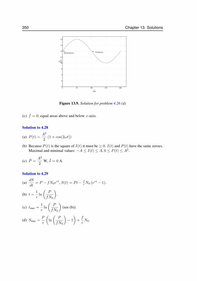
350 Chapter 13. Solutions
0 91 182 273 3640
2
4
6
8
10
12
14
16
tdays
l(t)
ho
urs
Spring Equinox Fall Equinox
Figure 13.9. Solution for problem 4.26 (d)
(c) f = 0; equal areas above and below x-axis.
Solution to 4.28
(a) P (t) =A2
2(1 + cos(2ωt))
(b) Because P (t) is the square of I(t) it must be≥ 0. I(t) and P (t) have the same zeroes.Maximal and minimal values: −A ≤ I(t) ≤ A, 0 ≤ P (t) ≤ A2.
(c) P =A2
2W, I = 0 A.
Solution to 4.29
(a)dS
dt= P − fN0e
rt, S(t) = Pt− frN0 (ert − 1).
(b) t =1
rln
(P
fN0
).
(c) tmax =1
rln
(P
fN0
)(see (b)).
(d) Smax =P
r
(ln
(P
fN0
)− 1
)+f
rN0.
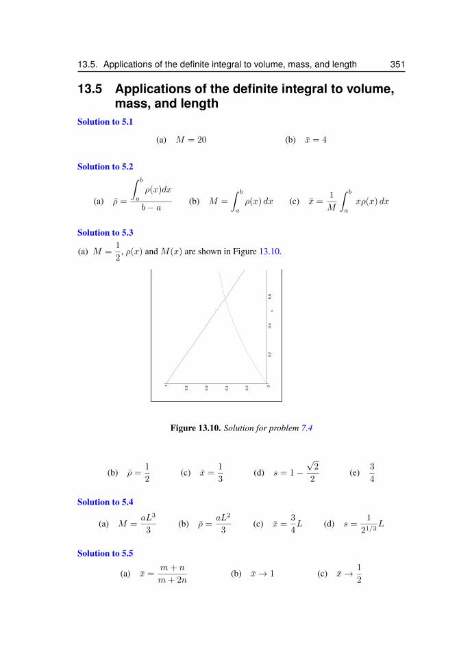
13.5. Applications of the definite integral to volume, mass, and length 351
13.5 Applications of the definite integral to volume,mass, and length
Solution to 5.1
(a) M = 20 (b) x = 4
Solution to 5.2
(a) ρ =
∫ b
a
ρ(x)dx
b− a(b) M =
∫ b
a
ρ(x) dx (c) x =1
M
∫ b
a
xρ(x) dx
Solution to 5.3
(a) M =1
2, ρ(x) and M(x) are shown in Figure 13.10.
0
0.2
0.4
0.6
0.8
1
0.2
0.4
0.6
0.8
x
Figure 13.10. Solution for problem 7.4
(b) ρ =1
2(c) x =
1
3(d) s = 1−
√2
2(e)
3
4
Solution to 5.4
(a) M =aL3
3(b) ρ =
aL2
3(c) x =
3
4L (d) s =
1
21/3L
Solution to 5.5
(a) x =m+ n
m+ 2n(b) x→ 1 (c) x→ 1
2
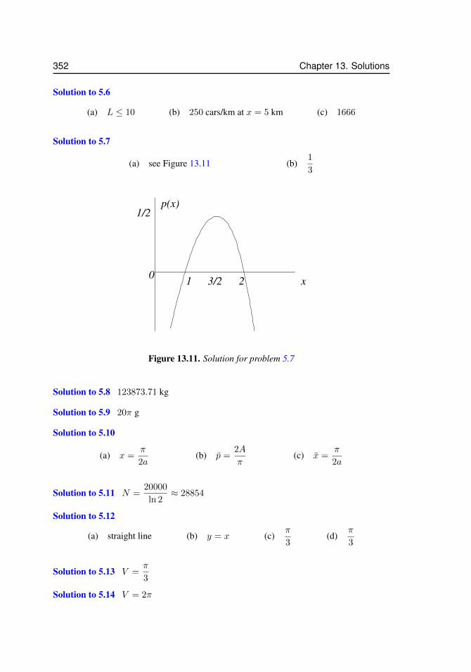
352 Chapter 13. Solutions
Solution to 5.6
(a) L ≤ 10 (b) 250 cars/km at x = 5 km (c) 1666
Solution to 5.7
(a) see Figure 13.11 (b)1
3
3/2 x
p(x)
0
1/2
1 2
Figure 13.11. Solution for problem 5.7
Solution to 5.8 123873.71 kg
Solution to 5.9 20π g
Solution to 5.10
(a) x =π
2a(b) p =
2A
π(c) x =
π
2a
Solution to 5.11 N =20000
ln 2≈ 28854
Solution to 5.12
(a) straight line (b) y = x (c)π
3(d)
π
3
Solution to 5.13 V =π
3
Solution to 5.14 V = 2π
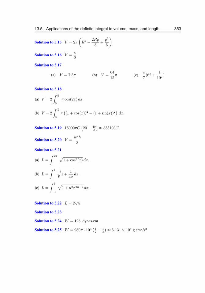
13.5. Applications of the definite integral to volume, mass, and length 353
Solution to 5.15 V = 2π
(R2 − 2Rp
3+p2
5
)Solution to 5.16 V =
π
2
Solution to 5.17
(a) V = 7.5π (b) V =64
15π (c)
π
7(62 +
1
107)
Solution to 5.18
(a) V = 2
∫ π4
0
π cos(2x) dx.
(b) V = 2
∫ π4
0
π((1 + cos(x))2 − (1 + sin(x))2
)dx.
Solution to 5.19 16000πC(20− 40
3
)≈ 335103C
Solution to 5.20 V =w2h
3
Solution to 5.21
(a) L =
∫ 2π
0
√1 + cos2(x) dx.
(b) L =
∫ 1
0
√1 +
1
4xdx.
(c) L =
∫ 1
−1
√1 + n2x2n−2 dx.
Solution to 5.22 L = 2√
5
Solution to 5.23
Solution to 5.24 W = 128 dynes·cm
Solution to 5.25 W = 980π · 103(
12 −
13
)≈ 5.131× 10⁵ g cm2/s2
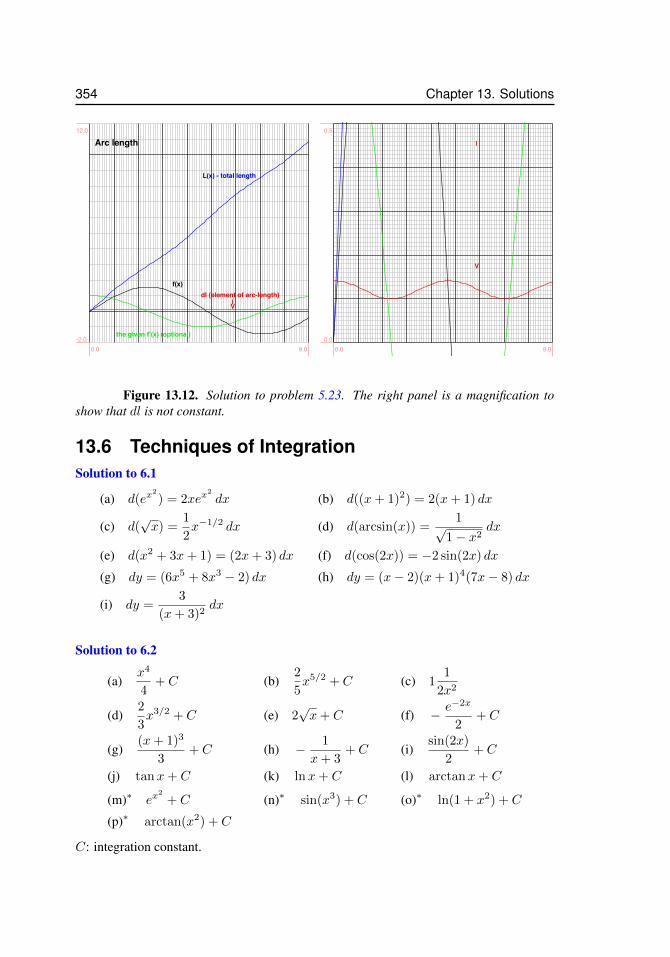
354 Chapter 13. Solutions
the given f’(x) (optional)
f(x)dl (element of arc-length)
V|
L(x) - total length
Arc length
0.0 9.0-2.0
12.0
V
|
0.0 9.00.0
0.5
Figure 13.12. Solution to problem 5.23. The right panel is a magnification toshow that dl is not constant.
13.6 Techniques of IntegrationSolution to 6.1
(a) d(ex2
) = 2xex2
dx (b) d((x+ 1)2) = 2(x+ 1) dx
(c) d(√x) =
1
2x−1/2 dx (d) d(arcsin(x)) =
1√1− x2
dx
(e) d(x2 + 3x+ 1) = (2x+ 3) dx (f) d(cos(2x)) = −2 sin(2x) dx
(g) dy = (6x5 + 8x3 − 2) dx (h) dy = (x− 2)(x+ 1)4(7x− 8) dx
(i) dy =3
(x+ 3)2dx
Solution to 6.2
(a)x4
4+ C (b)
2
5x5/2 + C (c) 1
1
2x2
(d)2
3x3/2 + C (e) 2
√x+ C (f) − e−2x
2+ C
(g)(x+ 1)3
3+ C (h) − 1
x+ 3+ C (i)
sin(2x)
2+ C
(j) tanx+ C (k) lnx+ C (l) arctanx+ C
(m)∗ ex2
+ C (n)∗ sin(x3) + C (o)∗ ln(1 + x2) + C
(p)∗ arctan(x2) + C
C: integration constant.
13.6. Techniques of Integration 355
Solution to 6.3
(a)
(i) − cos(3x)
3+ C (ii) 2 sin(
√x) + C
(iii)1
6(x4 + 1)3/2 + C (iv) 2 ln |1 + 2x|+ C
(b)
(i) ≈ 13.89 (ii)1
2(iii) 0
Solution to 6.4
(a) arctan(p)− π
4(b)
1
21(x3 + 1)7 + C (c)
1
3(1 + 2ex)3/2 + C
(d) ln | ln |x||+ C (e) − ln |1− y|+ C (f) k1 ln
∣∣∣∣ k2 − 1
k2 − S
∣∣∣∣(g) − 1
3ln∣∣1− x3
∣∣+ C (h)2
9(3x+ 1)3/2 + C (i)
√4 + x2 + C
(j)1
6sin6 x+ C (k)
3
5ln |4 + 5x|+ C (l) ln | sin(θ)|+ C
(m) 2(2 + tanx)1/2 + C (n) arctan(x
2) + C
Solution to 6.51
2sin2 x+ C
Solution to 6.6
(a) substitute x = sin(u).
(b) I =1
2
∫(1 + cos(2u)) du ⇒ I =
1
2(arcsinx+ x
√1− x2)
∣∣10
=π
4.
(c) f(x) =√
1− x2 forms a half-circle of radius 1 for −1 < x < 1.
Solution to 6.7
(a)1
9ln
∣∣∣∣x− 5
x+ 4
∣∣∣∣+ C (b) − 3
x+ 3+ C
(c) − 1√10
arctan
(x+ 2√
10
)+ C (d) ln
∣∣∣∣x− 4
x− 2
∣∣∣∣+ C
Solution to 6.8
(a)1
aarctan
(xa
)+ C (b)
1
2aln
∣∣∣∣a+ x
a− x
∣∣∣∣+ C

356 Chapter 13. Solutions
Solution to 6.9 Set u = xn and dv = ex.
Solution to 6.10
(a) − 2√x cos
(√x)
+ 2 sin(√x)
+ C (b) 2e2
(c) − π
4− 1
2(d)
1
2ex
2 (x4 − 2x2 + 2
)+ C
Solution to 6.11
(a)3√2
arctan
(x+ 2√
2
)+ C (b) 2 ln
∣∣∣∣x+ 1
x+ 2
∣∣∣∣+ C (c)1
2ln
∣∣∣∣x+ 2
x+ 4
∣∣∣∣+ C
(d) DNE (e)1
4
(1− 2Te−2T − e−2T
)(f) 4
(g) ln |x|x3
3− x3
9+ C
DNE: does not exist.
13.6. Techniques of Integration 357
Solution to 6.12
(1)ln(x)2
2+ C (2)
2
3ln |2 + 3x|+ C
(3) − 1
9cos(3x3 + 1) + C (4)
1
3
(e12 − e3
)(5)
1
2ln 2 (6)
1√3
arcsin
(√6
2x
)+ C
(7)1√3
arctan
(2x√
3
)+ C (8)
1
2arcsin
(2x
5
)+ C
(9)√
9 + x2 + C (10) − 1
6(sin2(3x)− 2 sin(3x)) + C
(11)sin(2x)
2+
cos(4x)
8+ C (12)
2
3(tanx+ 1)3/2 + C
(13)1
3(14) x2 + x cos(2x)− sin(2x)
2+ C
(15) secx+ C (16) − x cos(x+ 1) + sin(x+ 1) + C
(17)x6
6+ C (18) tan t+ C
(19) − 1
2(x+ 3)+ C (20)
1
6ln
∣∣∣∣x− 5
x+ 1
∣∣∣∣+ C
(21) − 1
7ln
∣∣∣∣ x+ 3
2x− 1
∣∣∣∣+ C (22) ln
∣∣∣∣x+ 2
x+ 3
∣∣∣∣+ C
(23) − 1
x3 + x+ C (24) ln
∣∣∣∣x− 2
x− 1
∣∣∣∣+ C
(25)2√
51
17arctan
(1√51
(2x+ 3)
)+ C (26) x tanx+ ln | cosx|+ C
(27)1
2ex
2
+ C (28) ex(x2 − 2x+ 2) + C
(29) x arctanx− 1
2ln(1 + x2) + C (30)
ex
2(x cosx+ x sinx− sinx) + C
Solution to 6.13 V =2
3π
Solution to 6.14
(a) M =1
a(1− e−aL) (b) p =
1
aL(1− e−aL) (c) x =
aL e−aL + e−aL − 1
a(e−aL − 1)
Solution to 6.15 x =π
4.

358 Chapter 13. Solutions
Solution to 6.16
(a) M = βa2π
4(b) x =
4a
3π
Solution to 6.17
(a) See Figure 13.13 (b) xc = 2
(c) Mc = −10e−3/2 + 6e−1/2 (d) x =2− 7e−5/2
8− 53e−5/2≈ 2.56
0
0.1
0.2
0.3
0.4
0.5
0.6
0.7
1 2 3 4 5x
Figure 13.13. Solution for problem 7.11.
Solution to 6.18 L =1
27(13√
13− 8) ≈ 1.44
Solution to 6.19
(a) F (x) (b) statement is true
(c) L =
∫ 1
0
√1 + x2 dx (d) substitution does indeed the trick
(e) L =1
2(√
2 + ln(1 +√
2)) ≈ 1.478
Solution to 6.20 V = 2π2r2R
Solution to 6.21 S =13
3π
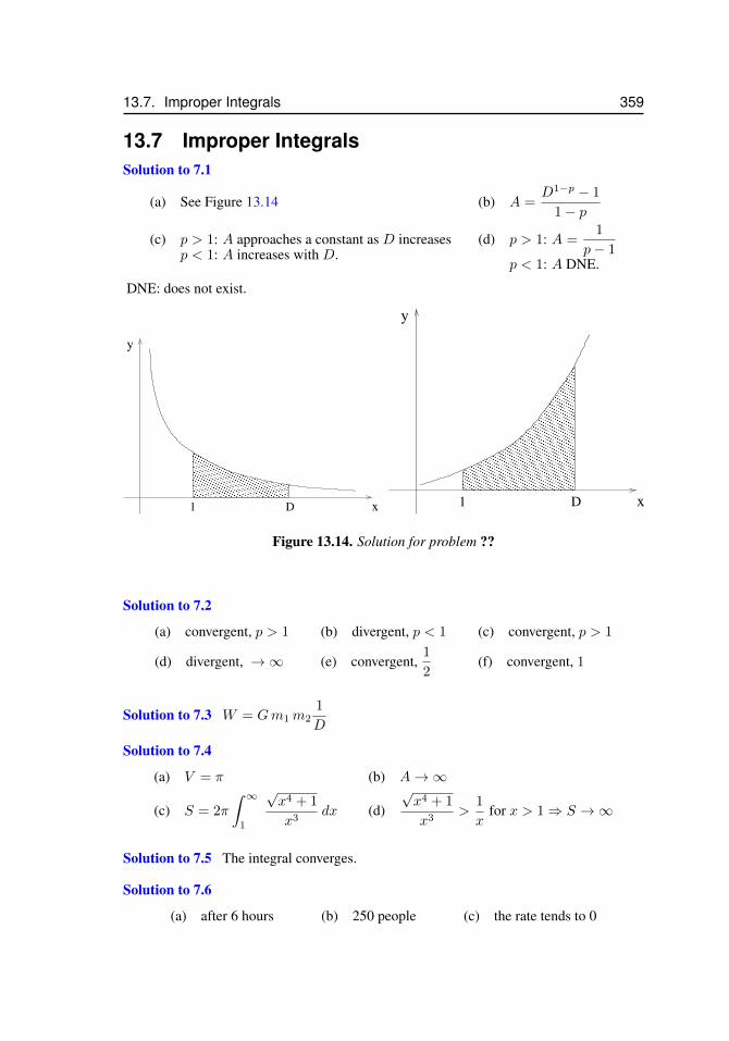
13.7. Improper Integrals 359
13.7 Improper IntegralsSolution to 7.1
(a) See Figure 13.14 (b) A =D1−p − 1
1− p
(c) p > 1: A approaches a constant as D increasesp < 1: A increases with D.
(d) p > 1: A =1
p− 1p < 1: A DNE.
DNE: does not exist.
������������������������������������������������������������������������������������������
������������������������������������������������������������������������������������������
x
y
1 D
������������������������������������������������������������������������������������������������������������������������������������������������������������������������������������������������������������������
������������������������������������������������������������������������������������������������������������������������������������������������������������������������������������������������������������������
D1 x
y
Figure 13.14. Solution for problem ??
Solution to 7.2
(a) convergent, p > 1 (b) divergent, p < 1 (c) convergent, p > 1
(d) divergent, →∞ (e) convergent,1
2(f) convergent, 1
Solution to 7.3 W = Gm1m21
D
Solution to 7.4
(a) V = π (b) A→∞
(c) S = 2π
∫ ∞1
√x4 + 1
x3dx (d)
√x4 + 1
x3>
1
xfor x > 1⇒ S →∞
Solution to 7.5 The integral converges.
Solution to 7.6
(a) after 6 hours (b) 250 people (c) the rate tends to 0
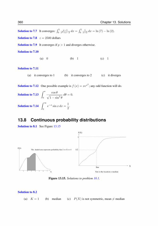
360 Chapter 13. Solutions
Solution to 7.7 It converges:∫ 5
0x−1
x2+x−2 dx =∫ 5
01
x+2 dx = ln (7)− ln (2).
Solution to 7.8 z = 2500 dollars
Solution to 7.9 It converges if p > 1 and diverges otherwise.
Solution to 7.10
(a) 0 (b) 1 (c) 1
Solution to 7.11
(a) it converges to 1 (b) it converges to 2 (c) it diverges
Solution to 7.12 One possible example is f (x) = xex2
; any odd function will do.
Solution to 7.13∫ π
0
cos θ√1− sin3 θ
dθ = 0.
Solution to 7.14∫ ∞
0
e−x sinx dx =1
2.
13.8 Continuous probability distributionsSolution to 8.1 See Figure 13.15
����������������
����������������
���������������������
���������������������
1 2 3 4 5 6 7
The shaded area represents probability that 2 <= X <= 4P(X)
X
F(X)
1
1/2
XmX
Xm is the location o median
Figure 13.15. Solutions to problem 10.1.
Solution to 8.2
(a) K = 1 (b) median (c) P (X) is not symmetric, mean 6= median
13.8. Continuous probability distributions 361
Solution to 8.3 The cumulative probability distribution, F (x), for a < x < b denotes theprobability that the outcome lies in [a, x].
Solution to 8.4
(a) C =e
10(e− 1)≈ 0.158 (b) hard, density highest at low end.
Solution to 8.5
(a) C =1
2b, F (x) =
x+ b
2b(b) C =
3
4b3, F (x) =
x3 − 3b2x− 2b3
2b3
Solution to 8.6
(a) m = 0 (b) m = 1−√
2 (c) m = 5
(1− 1√
2
)(d) m =
π
6
Solution to 8.7
(a) p2 < p1 < p3 (b) m2 < m1 < m3
Solution to 8.8
(a) more below sea level (b) ≈ 3
4
Solution to 8.9
(a) Because p(x) is normalized and the median cuts the distribution into two equal propor-tions, each has to be 1/2.
(b) x = m = 50. With 50% chance a student scores better than the mean or median of 50points. A median of 50 points is generally fairly low and so many students found thecourse hard.
(c) C =1
5000, x =
200
3≈ 66.667,m =
√5000 ≈ 70.71. The chance that a student did
better than the mean was 5/9. The chance to do better than the median is always 1/2(by definition). Half the class scored 70.71 points or better and hence the course waseasier than the one in (b).
Solution to 8.10
(a) 90% of all adult males are 200 cm or less.
(b) 20% of all adult males are between 150 cm to 160 cm tall.
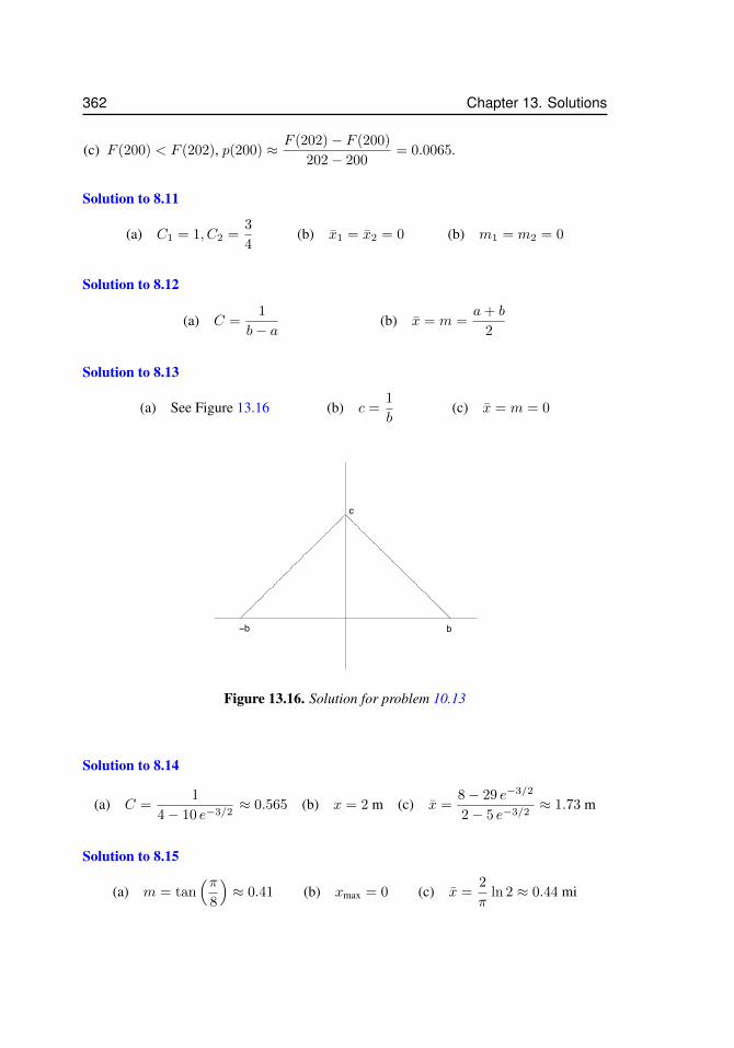
362 Chapter 13. Solutions
(c) F (200) < F (202), p(200) ≈ F (202)− F (200)
202− 200= 0.0065.
Solution to 8.11
(a) C1 = 1, C2 =3
4(b) x1 = x2 = 0 (b) m1 = m2 = 0
Solution to 8.12
(a) C =1
b− a(b) x = m =
a+ b
2
Solution to 8.13
(a) See Figure 13.16 (b) c =1
b(c) x = m = 0
−b b
c
Figure 13.16. Solution for problem 10.13
Solution to 8.14
(a) C =1
4− 10 e−3/2≈ 0.565 (b) x = 2 m (c) x =
8− 29 e−3/2
2− 5 e−3/2≈ 1.73 m
Solution to 8.15
(a) m = tan(π
8
)≈ 0.41 (b) xmax = 0 (c) x =
2
πln 2 ≈ 0.44 mi
13.8. Continuous probability distributions 363
Solution to 8.16
(a) C =3
520300≈ 5.766 · 10−6 (b)
8060
3C ≈ 1.549 · 10−2
(c) ≈ 43% (d) ≈ 78.83 years
Solution to 8.17
(a) p(x) =π
6cos(π
6x)
(b) x = 0 (c) x = 3π − 2
π, m = 1
(d) & (e) not shown
Solution to 8.18
(a)∫ ∞
0
f(x) dx = 1 and f(x) ≥ 0 for x ≥ 0 (b)21
100
Solution to 8.19
(a) C =1
10(b) F (t) = 1− e−t/10 (c) e−2 ≈ 13.53% (d) t = 10 days
Solution to 8.20
(a) t = 20 +1
R(b) e−20R
Solution to 8.21
(a) C = 1,3
10(b) F (x) =
x
1 + x(c) see Figure 13.17
Solution to 8.22
(a) C =1
10(1− e−1)≈ 0.158 (b) x = 10 m,m = 10 ln
(2
1 + e−1
)≈ 3.799
(c) V = 100 (d) 1− e−0.1 ≈ 9.5%
Solution to 8.23 C = −1
2ln(0.7) ≈ 0.178
Solution to 8.24
(a) p(x) =1
3, F (x) =
1
3(x− 1), 1 ≤ x ≤ 4 (b) F (V ) =
1
3(V 1/3 − 1), 1 ≤ V ≤ 43
(c) p(V ) =1
9V −2/3, 1 ≤ V ≤ 43 (d) V =
85
4= 21.25 mm3
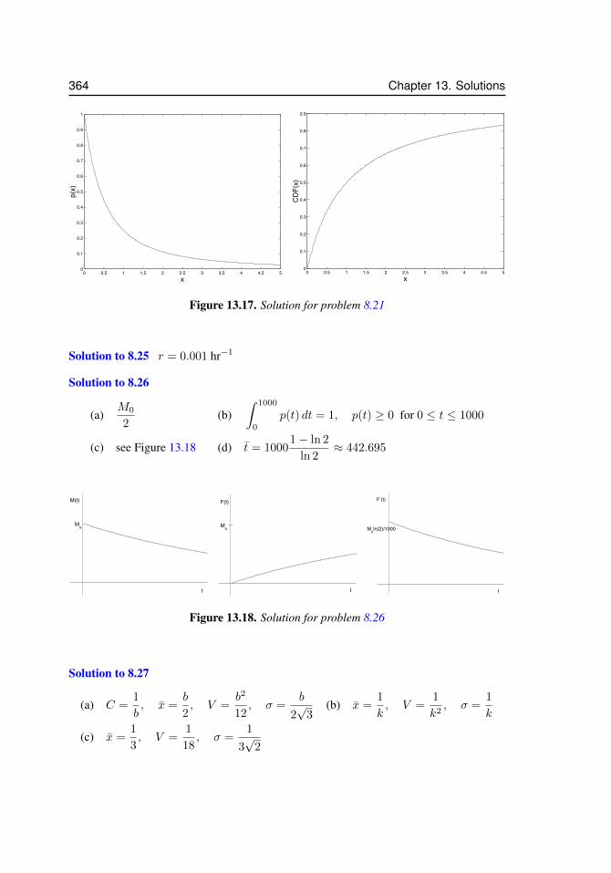
364 Chapter 13. Solutions
0 0.5 1 1.5 2 2.5 3 3.5 4 4.5 50
0.1
0.2
0.3
0.4
0.5
0.6
0.7
0.8
0.9
1
x
p(x)
0 0.5 1 1.5 2 2.5 3 3.5 4 4.5 50
0.1
0.2
0.3
0.4
0.5
0.6
0.7
0.8
0.9
x
CDF(x)
Figure 13.17. Solution for problem 8.21
Solution to 8.25 r = 0.001 hr−1
Solution to 8.26
(a)M0
2(b)
∫ 1000
0
p(t) dt = 1, p(t) ≥ 0 for 0 ≤ t ≤ 1000
(c) see Figure 13.18 (d) t = 10001− ln 2
ln 2≈ 442.695
Mo
t
M(t)
t
F(t)
Mo
t
Fv(t)
Moln(2)/1000
Figure 13.18. Solution for problem 8.26
Solution to 8.27
(a) C =1
b, x =
b
2, V =
b2
12, σ =
b
2√
3(b) x =
1
k, V =
1
k2, σ =
1
k
(c) x =1
3, V =
1
18, σ =
1
3√
2
13.9. Differential Equations 365
Solution to 8.28
(a) V =(b− a)2
12, σ =
b− a2√
3(b) F (x) =
x− ab− a
Solution to 8.29 V =b2
6, σ =
b√6
Solution to 8.30
(a) C =π
12(b) I0 = 1, I1 = 3, I2 = 18
π2 − 4
π2(c) V = 9
π2 − 8
π2, σ =
√V
Solution to 8.31
(a) C =1√2π
(b) f(x) is even (c) V = σ = 1
Solution to 8.32
(a) reduce to integral in problem 8.31 (b) mean and median at z = 0 or x = µ
(c) M2 = σ2 + µ2 ⇒ V = σ2 (d) x = µ
Solution to 8.33
(a)∫ ∞
0
p(r) dr = 1 and p(r) ≥ 0 for0 ≤ x <∞
(b) p(0) = 0, rmin = 0, rmax = 1, limr→∞
p(r) = 0, see Figure 13.19
(c) r = 1 (d) µ =3
2
(e) F (r) = 1− (1 + 2r + 2r2)e−2r, F (1) = 1− 5e−2 ≈ 32%
13.9 Differential EquationsSolution to 9.1
(a) y(t) = 10e−t2
(b) y(t) =1
1 + e−t
Solution to 9.2
(a) y(t) = 1− C e−t (b) C =1
2
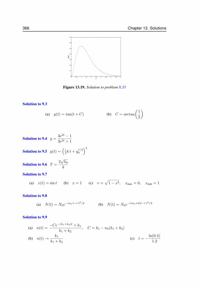
366 Chapter 13. Solutions
0 0.5 1 1.5 2 2.5 3 3.5 4 4.5 50
0.1
0.2
0.3
0.4
0.5
0.6
0.7
r
p(r)
Figure 13.19. Solution to problem 8.33
Solution to 9.3
(a) y(t) = tan(t+ C) (b) C = arctan
(1
2
)
Solution to 9.4 y =3e2t − 1
3e2t + 1
Solution to 9.5 y(t) =(
13k t+ y
1/30
)3
Solution to 9.6 T =2√h0
k
Solution to 9.7
(a) x(t) = sin t (b) x = 1 (c) v =√
1− x2, xmax = 0, xmin = 1
Solution to 9.8
(a) N(t) = N0e−m0 t−r t2/2 (b) N(t) = N0e
−(m0+b)t−r t2/2
Solution to 9.9
(a) n(t) =−Ce−(k1+k2)t + k1
k1 + k2, C = k1 − n0(k1 + k2)
(b) n(t)→ k1
k1 + k2(c) t = − ln(0.4)
1.2
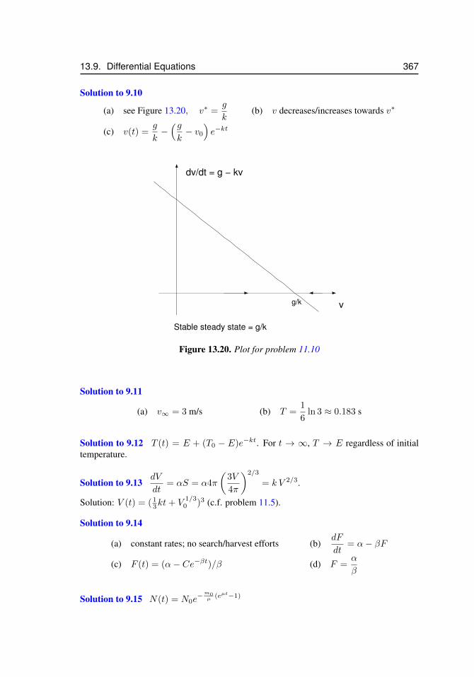
13.9. Differential Equations 367
Solution to 9.10
(a) see Figure 13.20, v∗ =g
k(b) v decreases/increases towards v∗
(c) v(t) =g
k−(gk− v0
)e−kt
dv/dt = g − kv
v
Stable steady state = g/k
g/k
Figure 13.20. Plot for problem 11.10
Solution to 9.11
(a) v∞ = 3 m/s (b) T =1
6ln 3 ≈ 0.183 s
Solution to 9.12 T (t) = E + (T0 − E)e−kt. For t → ∞, T → E regardless of initialtemperature.
Solution to 9.13dV
dt= αS = α4π
(3V
4π
)2/3
= k V 2/3.
Solution: V (t) = ( 13kt+ V
1/30 )3 (c.f. problem 11.5).
Solution to 9.14
(a) constant rates; no search/harvest efforts (b)dF
dt= α− βF
(c) F (t) = (α− Ce−βt)/β (d) F =α
β
Solution to 9.15 N(t) = N0e−m0
µ (eµt−1)
368 Chapter 13. Solutions
Solution to 9.16
(a) N(t) = 2(t+ 1) (b) N(t) =2(t+ 1)
t− 1
(c) C(t+ 1) 6= 1 must hold – true because 0 ≤ C = 1− 1
N0< 1
13.10 SequencesSolution to 10.1
(a) divergent (b) convergent (c) convergent(d) convergent (e) divergent (f) divergent
Solution to 10.2 The sequence is convergent, and its limit is 0.
Solution to 10.3 The sequence is convergent, and its limit is 1.
Solution to 10.4
(a) monotonically decreasing, bounded (b) bounded, not monotonic(c) neither bounded nor monotonic (d) monotonically decreasing, bounded
Solution to 10.5 ≈ 11.9 years; after n years, the balance is 1000 (1.06)n
Solution to 10.6 The formula is ak = 1 + 3k, and a30 = 91.
Solution to 10.7 In the kth division, the first person eats(
13
) (23
)2kof the pie and the
second person eats(
13
) (23
)2k+1of the pie.
Solution to 10.8
(a) diverges (b) converges (to 1/2)
Solution to 10.9 The sequence is monotone decreasing, bounded from above by 2, andfrom below by 1.
Solution to 10.10 {xn}n>0 satisfies xn+1 =2x3
n + a
3x2n
. If x0 = a = 2, then the first
several terms in this sequence are 2, 3/2, 35/27, 125116/99225, . . . .
Solution to 10.11 The fixed point is x∗ ≈ 1.2237.
Solution to 10.12 Your pay for the nth hour of work is an = 7 + 0.20 (n− 1), so yourpay for the last hour of the week is a40 = 14.80.
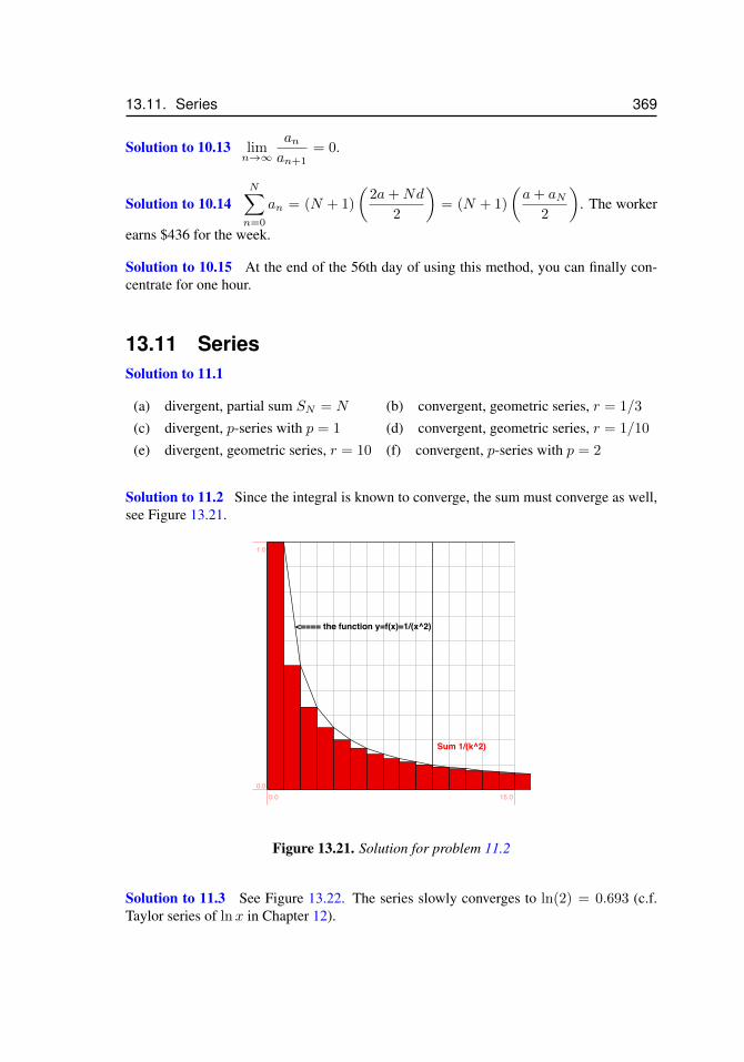
13.11. Series 369
Solution to 10.13 limn→∞
anan+1
= 0.
Solution to 10.14N∑n=0
an = (N + 1)
(2a+Nd
2
)= (N + 1)
(a+ aN
2
). The worker
earns $436 for the week.
Solution to 10.15 At the end of the 56th day of using this method, you can finally con-centrate for one hour.
13.11 SeriesSolution to 11.1
(a) divergent, partial sum SN = N (b) convergent, geometric series, r = 1/3
(c) divergent, p-series with p = 1 (d) convergent, geometric series, r = 1/10
(e) divergent, geometric series, r = 10 (f) convergent, p-series with p = 2
Solution to 11.2 Since the integral is known to converge, the sum must converge as well,see Figure 13.21.
<==== the function y=f(x)=1/(x^2)
Sum 1/(k^2)
0.0 15.00.0
1.0
Figure 13.21. Solution for problem 11.2
Solution to 11.3 See Figure 13.22. The series slowly converges to ln(2) = 0.693 (c.f.Taylor series of lnx in Chapter 12).
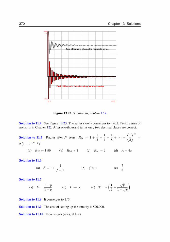
370 Chapter 13. Solutions
First 100 terms in the alternating harmonic series
Sum of terms in alternating harmonic series
0.0 100.0-0.5
1.0
Figure 13.22. Solution to problem 11.4
Solution to 11.4 See Figure 13.23. The series slowly converges to π (c.f. Taylor series ofarctanx in Chapter 12). After one-thousand terms only two decimal places are correct.
Solution to 11.5 Radius after N years: RN = 1 +1
2+
1
4+
1
8+ · · · +
(1
2
)N=
2(1− 2−N−1
).
(a) R20 ≈ 1.99 (b) R50 ≈ 2 (c) R∞ = 2 (d) A = 4π
Solution to 11.6
(a) S = 1 +4
f − 1(b) f > 1 (c)
7
3
Solution to 11.7
(a) D =1 + p
1− p(b) D →∞ (c) T = k
(1
2+
√p
1−√p
)
Solution to 11.8 It converges to 1/3.
Solution to 11.9 The cost of setting up the annuity is $20,000.
Solution to 11.10 It converges (integral test).
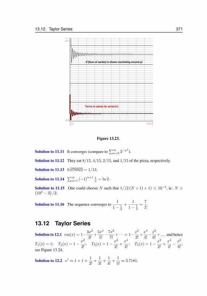
13.12. Taylor Series 371
Terms in series for arctan(1)
4*[Sum of series] is shown oscillating around pi
0.0 100.0-0.4
4.0
Figure 13.23.
Solution to 11.11 It converges (compare to∑∞n=0 2−n
2
).
Solution to 11.12 They eat 8/15, 4/15, 2/15, and 1/15 of the pizza, respectively.
Solution to 11.13 0.076923 = 1/13.
Solution to 11.14∑∞n=1 (−1)
n+1 1n = ln 2.
Solution to 11.15 One could choose N such that 1/ (2 (N + 1) + 1) < 10−3, ie. N >(103 − 3
)/2.
Solution to 11.16 The sequence converges to1
1− 12
+1
1− 13
=7
2.
13.12 Taylor Series
Solution to 12.1 cos(x) = 1− 3x2
3!+
5x4
5!− 7x6
7!+· · · = 1−x
2
2!+x4
4!−x
6
6!+. . . and hence
T1(x) = 1; T2(x) = 1− x2
2!; T3(x) = 1− x2
2!+x4
4!; T4(x) = 1− x2
2!+x4
4!− x6
6!,
see Figure 13.24.
Solution to 12.2 e1 ≈ 1 + 1 +1
2!+
1
3!+
1
4!+
1
5!≈ 2.7181.
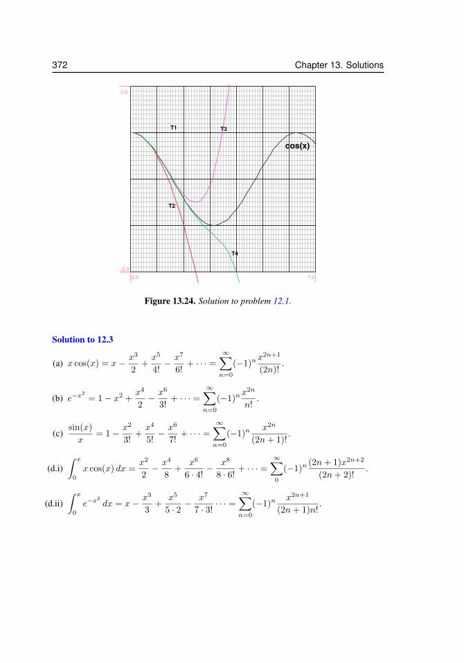
372 Chapter 13. Solutions
cos(x)
T1
T2
T3
T4
0.0 7.0-2.0
2.0
Figure 13.24. Solution to problem 12.1.
Solution to 12.3
(a) x cos(x) = x− x3
2+x5
4!− x7
6!+ · · · =
∞∑n=0
(−1)nx2n+1
(2n)!.
(b) e−x2
= 1− x2 +x4
2− x6
3!+ · · · =
∞∑n=0
(−1)nx2n
n!.
(c)sin(x)
x= 1− x2
3!+x4
5!− x6
7!+ · · · =
∞∑n=0
(−1)nx2n
(2n+ 1)!.
(d.i)∫ x
0
x cos(x) dx =x2
2− x4
8+
x6
6 · 4!− x8
8 · 6!+ · · · =
∞∑0
(−1)n(2n+ 1)x2n+2
(2n+ 2)!.
(d.ii)∫ x
0
e−x2
dx = x− x3
3+
x5
5 · 2− x7
7 · 3!· · · =
∞∑n=0
(−1)nx2n+1
(2n+ 1)n!.
13.12. Taylor Series 373
Solution to 12.4
(a) e−x2/2 =
∞∑n=0
(−1)n
2nn!x2n (b) ln(1 + x) =
∞∑n=1
(−1)n−1
nxn
(c)√x sin
(√x)
=
∞∑n=0
(−1)n
(2n+ 1)!xn+1 (d)
ex + e−x
2=
∞∑n=0
1
(2n)!x2n
Solution to 12.5
(a)√
110 = 10√
1 + 0.1 ≈ 10.4875 (calculator: 10.488088).
(b) e0.1 = e0+0.1 ≈ 1.105 (calculator: 1.1051709).
(c) cos(3) = cos(π + (−0.14)) ≈ −0.9902 (calculator: −0.9899925).
(d) arctan(1.1) = arctan(1 + 0.1) ≈ 0.83289816 (calculator: 0.83298127).
Solution to 12.6
(a) x+1
3x3 (b) 1 + 2x+
3
2x2 +
2
3x3 +
5
24x4
(c) 1− 2x+ 3x2 − 10
3x3 (d) x2 − x4
3+
2x6
45
Solution to 12.7
(a) S =1
1 + x3=
∞∑n=0
(−1)nx3n (b) S =1
1 + t2=
∞∑n=0
(−1)nt2n
(c) S = arctan(x) =
∫ x
0
1
1 + t2dt =
∞∑n=0
(−1)nx2n+1
2n+ 1
Solution to 12.8
(a)e−t − 1
t=
∞∑n=1
(−1)n
n!tn−1 (b) E(x) =
∞∑n=1
(−1)nxn
n · n!
Solution to 12.9ex
xn>
x
(n+ 1)!. For fixed n, the lower bound becomes arbitrarily large
for x→∞ and hence ex must grow faster than xn for any n.
Solution to 12.10 F (x) =
∞∑n=1
(−1)n−1 x2n+1
n(2n+ 1).
374 Chapter 13. Solutions
Solution to 12.11 y(t) = 1 + (1 + b)t+1
2(1 + b)t2 +
1
6(1 + b)t3 + . . . .
Setting b = 0 yields y(t) = 1 + t+ 12 t
2 + 16 t
3 + · · · = et, as it should.
Solution to 12.12 y(t) = t− 1
3!t3 +
1
5!t5 + · · · = sin t.