integral boundary layer methods for wind turbine aerodynamics · integral boundary layer methods...

ECN-C--04-004

INTEGRAL BOUNDARY LAYERMETHODS FOR WIND TURBINE

AERODYNAMICS

A Literature Survey

A. van Garrel

December 2003

INTEGRAL BOUNDARY LAYER METHODS FOR WIND TURBINE AERODYNAMICS

Abstract

The simulation of wind turbine rotor aerodynamics can be improved upon by increasing thephysics content in the underlying approximations. The current effort is targeted at an aerody-namics model in which the flow field is decomposed into two domains. The inviscid externalflow domain is modeled with a “panel method” type of flow solver and the viscous regions aremodeled with an integral boundary layer model. For the simulation of separated flows the twomodels are coupled in strong interaction. The technology for the “panel method” flow solveris considered common knowledge and is not expected to raise serious problems during its de-velopment. In this report the possibilities and difficulties in the development of the integralboundary layer solver are investigated. The feasibility of the development of the rotor aero-dynamics simulation code is shown through a discussion of succesful integral boundary layerapproaches based on the conservation form of the boundary layer equations and the impact oftime-dependency and rotor blade rotation related terms on the system of equations. In additiona number of possible boundary layer velocity profiles is described. As a result the developmentof the targeted wind turbine rotor aerodynamics simulation code is recommended. Due to thevast amount of possible solution strategies it is advised to develop the boundary layer solver inclose cooperation with experts in the field of computational fluid dynamics.

Acknowledgement This report is part of the project “preRotorFlow” in which the possibil-ities and risks areas in the development of an integral boundary layer solver for windturbinerotor applications are investigated.

The project is partly funded by Novem, the Netherlands Agency for Energy and the Environ-ment, contract number 2020-02-13-20-008. Additional funding is provided by ECN, projectnumber 7.4188.

ii ECN-C--04-004

CONTENTS

NOMENCLATURE 1

1 INTRODUCTION 3

1.1 Context . . . . . . . . . . . . . . . . . . . . . . . . . . . . . . . . . . . . . . 3

1.2 Outline . . . . . . . . . . . . . . . . . . . . . . . . . . . . . . . . . . . . . . 4

2 THREE DIMENSIONAL BOUNDARY LAYER 5

2.1 Introduction . . . . . . . . . . . . . . . . . . . . . . . . . . . . . . . . . . . . 5

2.2 3D Integral Boundary Layer Formulation . . . . . . . . . . . . . . . . . . . . 5

2.3 Rotation and Time Dependency . . . . . . . . . . . . . . . . . . . . . . . . . . 11

3 CLOSURE RELATIONS 15

3.1 Introduction . . . . . . . . . . . . . . . . . . . . . . . . . . . . . . . . . . . . 15

3.2 Streamwise Flow . . . . . . . . . . . . . . . . . . . . . . . . . . . . . . . . . 15

3.3 Crossflow . . . . . . . . . . . . . . . . . . . . . . . . . . . . . . . . . . . . . 16

4 CONCLUSIONS AND RECOMMENDATIONS 19

4.1 Conclusions . . . . . . . . . . . . . . . . . . . . . . . . . . . . . . . . . . . . 19

4.2 Recommendations . . . . . . . . . . . . . . . . . . . . . . . . . . . . . . . . . 20

BIBLIOGRAPHY 21

ECN-C--04-004 iii


iv ECN-C--04-004

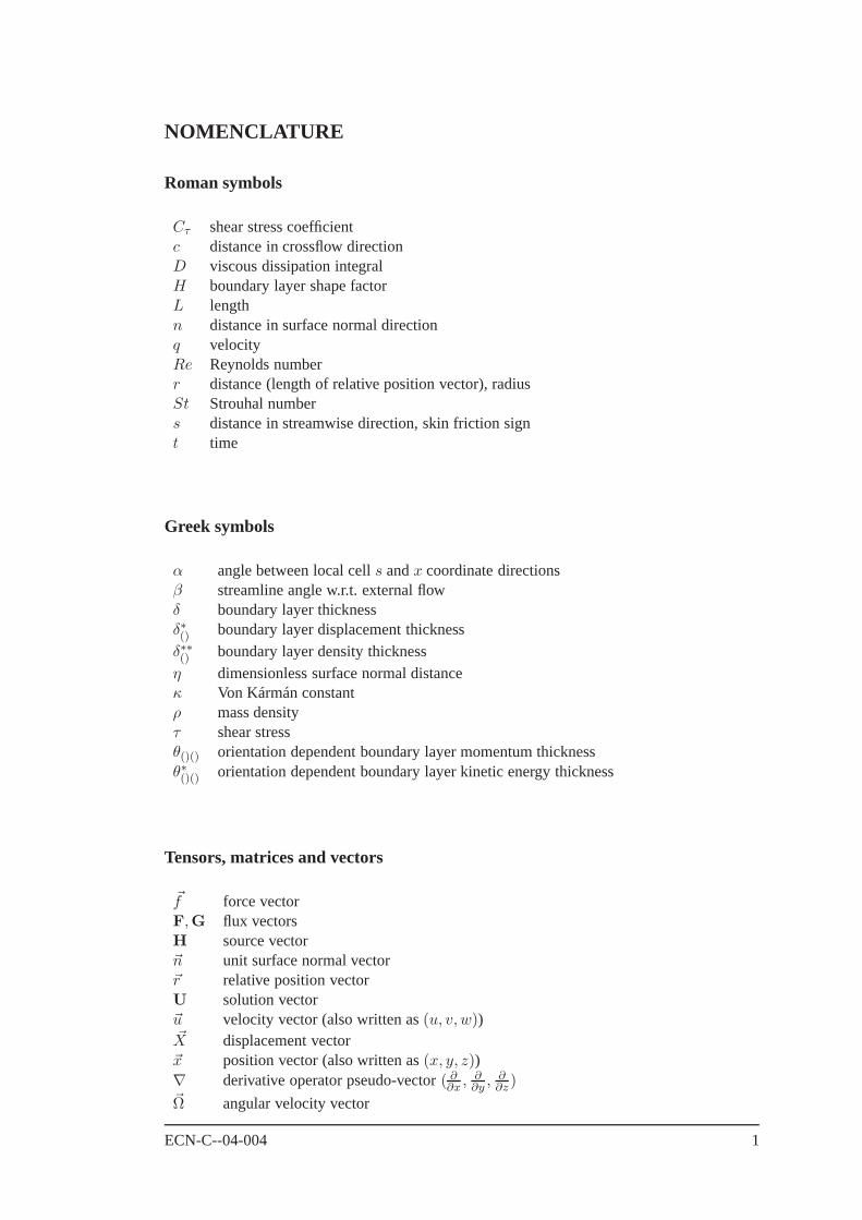
NOMENCLATURE

Roman symbols

Cτ shear stress coefficientc distance in crossflow directionD viscous dissipation integralH boundary layer shape factorL lengthn distance in surface normal directionq velocityRe Reynolds numberr distance (length of relative position vector), radiusSt Strouhal numbers distance in streamwise direction, skin friction signt time

Greek symbols

α angle between local cell s and x coordinate directionsβ streamline angle w.r.t. external flowδ boundary layer thicknessδ∗() boundary layer displacement thicknessδ∗∗() boundary layer density thicknessη dimensionless surface normal distanceκ Von Kármán constantρ mass densityτ shear stressθ()() orientation dependent boundary layer momentum thicknessθ∗()() orientation dependent boundary layer kinetic energy thickness

Tensors, matrices and vectors

f force vectorF,G flux vectorsH source vectorn unit surface normal vectorr relative position vectorU solution vectoru velocity vector (also written as (u, v,w))X displacement vectorx position vector (also written as (x, y, z))∇ derivative operator pseudo-vector ( ∂

∂x , ∂∂y , ∂

∂z )Ω angular velocity vector

ECN-C--04-004 1


Subscripts, superscripts and accents

()c value in crossflow direction()e value at the boundary layer edge()eq equilibrium value()n value or derivative in surface normal direction()ref reference value()s value in streamwise flow direction()w value at the wall()x value in x-direction()y value in y-direction() averaged quantity()′ fluctuating quantity

Acronyms

BC Boundary ConditionBL Boundary LayerCFD Computational Fluid DynamicsFEM Finite Element MethodFVM Finite Volume MethodIBL Integral Boundary LayerRANS Reynolds-Averaged Navier-StokesVII Viscous-Inviscid Interaction2D Two-Dimensional3D Three-Dimensional

2 ECN-C--04-004

1 INTRODUCTION

1.1 Context

The current trend in wind turbine design is towards larger and larger rotor diameters and anaccompanying increase in power output. Associated with this trend is a demand for moreaccurate and reliable wind turbine rotor aerodynamics simulation codes. The currently usedrotor aerodynamics simulation codes can roughly be subdivided into two groups of models,each with its own merits and disadvantages:

1. In the first group of simulation codes available aerodynamic data tables for two dimen-sional (2D) airfoils, for example obtained by wind tunnel experiments, form the basisof the method. Correction formulas are introduced to take into account the effects ofthe physics that are left out. Among the correction formulas are those that take into ac-count the influence of the rotor wake, the effects of yaw misalignment, dynamic inflow,dynamic stall and tip effects. The advantages of this group of codes are the very shortsimulation times and the low demand on user expertise making it possible to incorporatethem into structural dynamics simulation codes. The disadvantages are the inherent inac-curacies and uncertainties in the computed results introduced by the correction formulasand the little detailed information computed by the methods. This group of simulationcodes is used on a regular basis in wind turbine design practice.

2. The second group of simulation codes is based on a more fundamental description ofthe physics involved in time-dependent, three-dimensional, viscous flows around gen-eral configurations; the so called Reynolds averaged Navier-Stokes (RANS) equations.Only turbulence is approximated by a model. It should be noted that currently availableturbulence models are open to improvements for wind turbine rotor applications. Advan-tages are the general applicability of the method, the extensive amount of informationcomputed and the elimination of correction factors. Disadvantages are the great demandput on computer resources and the large effort required for input preparation and postprocessing. This group of rotor aerodynamics codes is currently used for isolated testcases in research environments where specialized expertise is available.

xxxxxxxxxxxxxxxxxxxxxxxxxxxxxxxxxxxxxxxxxxxxxxxxxxxxxxxxxxxxxxxxxxxxxxxxxxxxxxxxxxxxxxxxxxxxxxxxxxxxxxxxxxxxxxxxxxxxxxxxxxxxxxxxxxxxxxxxxxxxxxxxxxxxxxxxxxxxxxxxxxxxxxxxxxxxxxxxxxxxxxxxxxxxxxxxxxxxxxxxxxxxxxxxxxxxxxxxxxxxxxxxxxxxxxxxxxxxxxxxxxxxxxxxxxxxxxxxxxxxxxxxxxxxxxxxxxxxxxxxxxxxxxxxxxxxxxxxxxxxxxxxxxxxxxxxxxxxxxxxxxxxxxxxxxxxxxxxxxxxxxxxxxxxxxxxxxxxxxxxxxxxxxxxxxxxxxxxxxxxxxxxxxxxxxxxxxxxxxxxxxxxxxxxxxxxxxxxxxxxxxxxxxxxxxxxxxxxxxxxxxxxxxxxxxxxxxxxxxxxxxxxxxxxxxxxxxxxxxxxxxxxxxxxxxxxxxxxxxxxxxxxxxxxxxxxxxxxxxxxxxxxxxxxxxxxxxxxxxxxxxxxxxxxxxxxxxxxxxxxxxxxxxxxxxxxxxxxxxxxxxxxxxxxxxxxxxxxxxxxxxxxxxxxxxxxxxxxxxxxxxxxxxxxxxxxxxxxxxxxxxxxxxxxxxxxxxxxxxxxxxxxxxxxxxxxxxxxxxxxxxxxxxxxxxxxxxxxxxxxxxxxxxxxxxxxxxxxxxxxxxxxxxxxxxxxxxxxxxxxxxxxxxxxxxxxxxxxxxxxxxxxxxxxxxxxxxxxxxxxxxxxxxxxxxxxxxxxxxxx

Inviscid Flow

Viscous Flow

Figure 1: Flow domain decomposition into external inviscid flow and viscous boundary layerflow regions.

ECN-C--04-004 3


The goal of the current project is to investigate the technical possibilities and risk areas inthe development of a new wind turbine rotor aerodynamics simulation code that requires littleuser expertise and computer power, but can compute in detail the unsteady aerodynamic char-acteristics of rotor blades. The simulation of separated flow and the coupling with structuraldynamics simulation programs should be feasible.

This new rotor aerodynamics simulation program will be a combination of a “panel method”flow solver for the incompressible inviscid external flow and an integral boundary layer (IBL)solver for the three-dimensional (3D) viscous flow near the blade surface (see figure 1). Thestrong interaction between these two flow regimes in mildly separated flows will be accountedfor by a so called viscous-inviscid interaction (VII) algorithm. The viability of this approachwas confirmed positively by Veldman [40].

The technology for the “panel method” flow solver is considered common knowledge andis not expected to raise serious problems during its development. The feasibility of the de-velopment of the targeted rotor aerodynamics simulation code will be investigated through adiscussion of existing succesfull IBL approaches and the effects caused by the introduction oftime-dependency and rotor blade rotation related terms in the boundary layer equations.

1.2 Outline

In this project a large amount of literature on integral boundary layer theory was surveyed.It quickly became clear that the mathematics involved in the development of an IBL methodcapable of handling 3D separated flows about rotor blades, is of comparable complexity asthose in the development of a RANS code. Many of the choices and problems encounteredin the discretization of volume based RANS and Euler fluid dynamics codes transfer to theIBL equations also. A further obstacle was the large variation in notation schemes used in thevarious IBL articles.

Time constraints made it unfeasible to get, with the literature at hand, a complete roadmapor outline of the practical development of an IBL method for wind turbine rotor applications.As a result, in this report a concise survey is given of the available discretization and solutionschemes for IBL methods that have proven themselves in practical computations of separatedflows. Special attention is given to existing approaches for handling the effects introduced byblade rotation and unsteady flow features.

The current report makes significant use of the results from the research by Mughal reported in[20], [21] and the subsequent research by Nishida [24], [25], Milewski [19], Mughal [22] andCoenen [1].

The integral boundary layer equations and existing successful solution strategies are discussedin Chapter 2 together with the effects of introducing additional terms in the boundary layerequations to account for rotation and time dependency.

Some available velocity profile families for streamwise and crosswise laminar and turbulentflow are reported in Chapter 3.

In Chapter 4 some concluding remarks and recommendations regarding future developmentsare given.

4 ECN-C--04-004

2 THREE DIMENSIONAL BOUNDARY LAYER

2.1 Introduction

In this chapter existing solution methods for the 3D IBL equations are discussed. The effectsof rotation and translation of the frame of reference on the system of equations are indicatedtogether with the possibilities offered by the inclusion of time dependent terms. It shouldbe mentioned that the IBL equations included in this chapter serve as illustration along withthe text. No attempt is made to be complete in the definitions and describe the componentsin the boundary layer (BL) equations in detail. The interested reader is referred to the citedreferences.

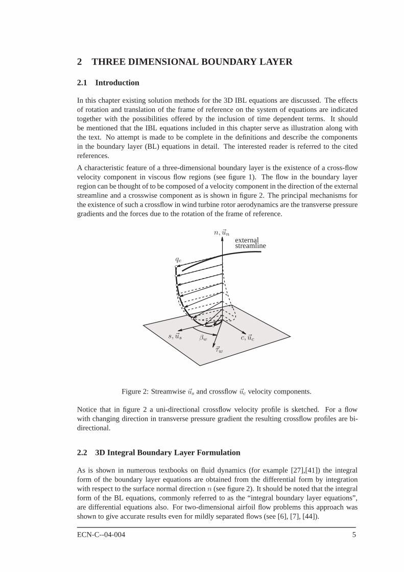
A characteristic feature of a three-dimensional boundary layer is the existence of a cross-flowvelocity component in viscous flow regions (see figure 1). The flow in the boundary layerregion can be thought of to be composed of a velocity component in the direction of the externalstreamline and a crosswise component as is shown in figure 2. The principal mechanisms forthe existence of such a crossflow in wind turbine rotor aerodynamics are the transverse pressuregradients and the forces due to the rotation of the frame of reference.

s, us c, uc

n, un

qe

τw

βw

externalstreamline

Figure 2: Streamwise us and crossflow uc velocity components.

Notice that in figure 2 a uni-directional crossflow velocity profile is sketched. For a flowwith changing direction in transverse pressure gradient the resulting crossflow profiles are bi-directional.

2.2 3D Integral Boundary Layer Formulation

As is shown in numerous textbooks on fluid dynamics (for example [27],[41]) the integralform of the boundary layer equations are obtained from the differential form by integrationwith respect to the surface normal direction n (see figure 2). It should be noted that the integralform of the BL equations, commonly referred to as the “integral boundary layer equations”,are differential equations also. For two-dimensional airfoil flow problems this approach wasshown to give accurate results even for mildly separated flows (see [6], [7], [44]).

ECN-C--04-004 5


The choice for an integral method formulation over a differential field method for the solutionof the 3D boundary layer equations is based on the following observations:

1. The combination of an IBL method formulation, a panel method solver for the externalflow and a viscous-inviscid interaction (VII) algorithm is more frequently encountered.

2. The IBL formulation can be shown to be hyperbolic in nature which facilitates the designof stable spatial discretization schemes. Integral methods tend to be more robust and arebetter suited for viscous-inviscid interaction.

3. The integral method formulation only requires a surface grid; possibly the same grid usedby the solver for the inviscid external flow. Field method BL solvers require a separatevolume grid around the domain of interest. Associated disadvantages are the increase inrequired user expertise for grid generation and the increase in number of unknowns tobe solved for.

4. There are more opportunities to tune the IBL method to measurements because of thedirect dependence on BL closure relationships. Field method BL solvers can be tunedonly indirectly through the turbulence model.

Prior to the solution method introduced in [20],[21], the IBL equations were mostly written ina finite difference curvi-linear formulation for non-orthogonal grids. The resulting equationsare analytically rather involved and contain a vast amount of metric coefficients and geodesiccurvature terms. Examples of this approach can be found in [2], [15], [23], [28], [30], [31] and[42].

Mughal, 1992

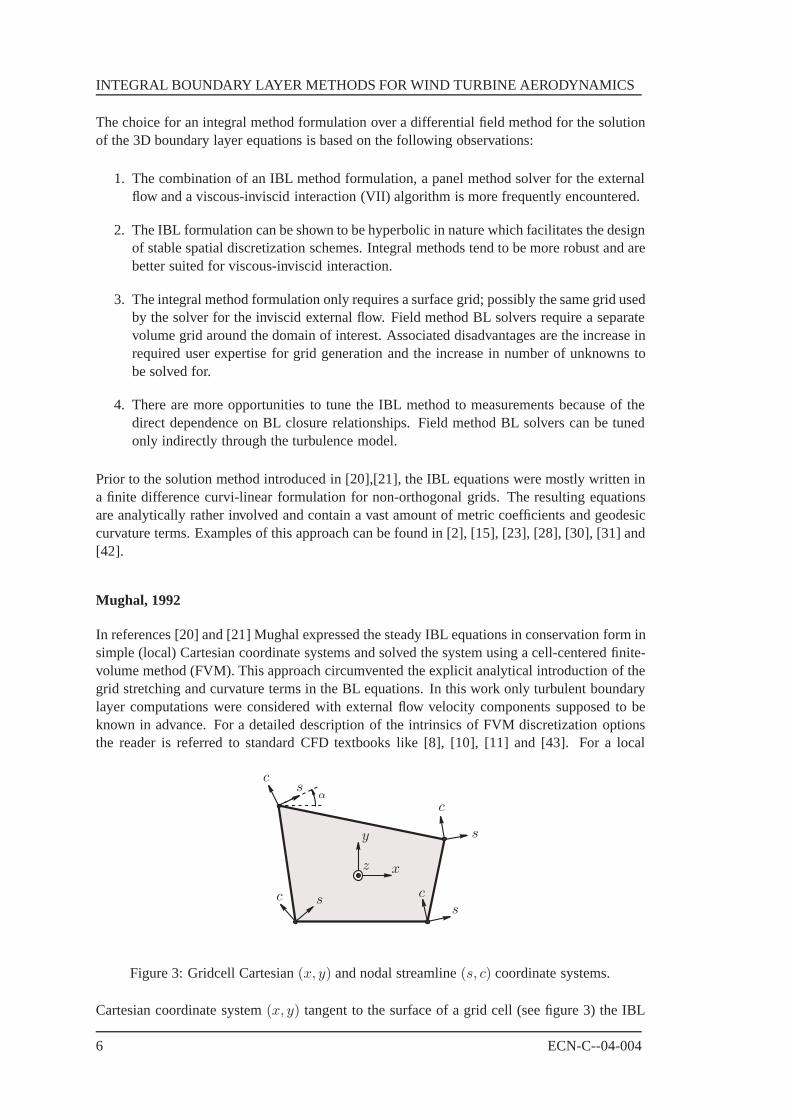
In references [20] and [21] Mughal expressed the steady IBL equations in conservation form insimple (local) Cartesian coordinate systems and solved the system using a cell-centered finite-volume method (FVM). This approach circumvented the explicit analytical introduction of thegrid stretching and curvature terms in the BL equations. In this work only turbulent boundarylayer computations were considered with external flow velocity components supposed to beknown in advance. For a detailed description of the intrinsics of FVM discretization optionsthe reader is referred to standard CFD textbooks like [8], [10], [11] and [43]. For a local

αs

ss

s

c

c

c

c

x

y

z

Figure 3: Gridcell Cartesian (x, y) and nodal streamline (s, c) coordinate systems.

Cartesian coordinate system (x, y) tangent to the surface of a grid cell (see figure 3) the IBL

6 ECN-C--04-004


equations read:

∂

∂x(ρeq

2eθxx) +

∂

∂y(ρeq

2eθxy) + ρeqeδ

∗x

∂ue

∂x+ ρeqeδ

∗y

∂ue

∂y= τwx , (1)

∂

∂x(ρeq

2eθyx) +

∂

∂y(ρeq

2eθyy) + ρeqeδ

∗x

∂ve

∂x+ ρeqeδ

∗y

∂ve

∂y= τwy , (2)

∂

∂x(ρeq

3eθ

∗x) +

∂

∂y(ρeq

3eθ

∗y) + ρeqeδ

∗∗x

∂q2e

∂x+ ρeqeδ

∗∗y

∂q2e

∂y= 2D. (3)

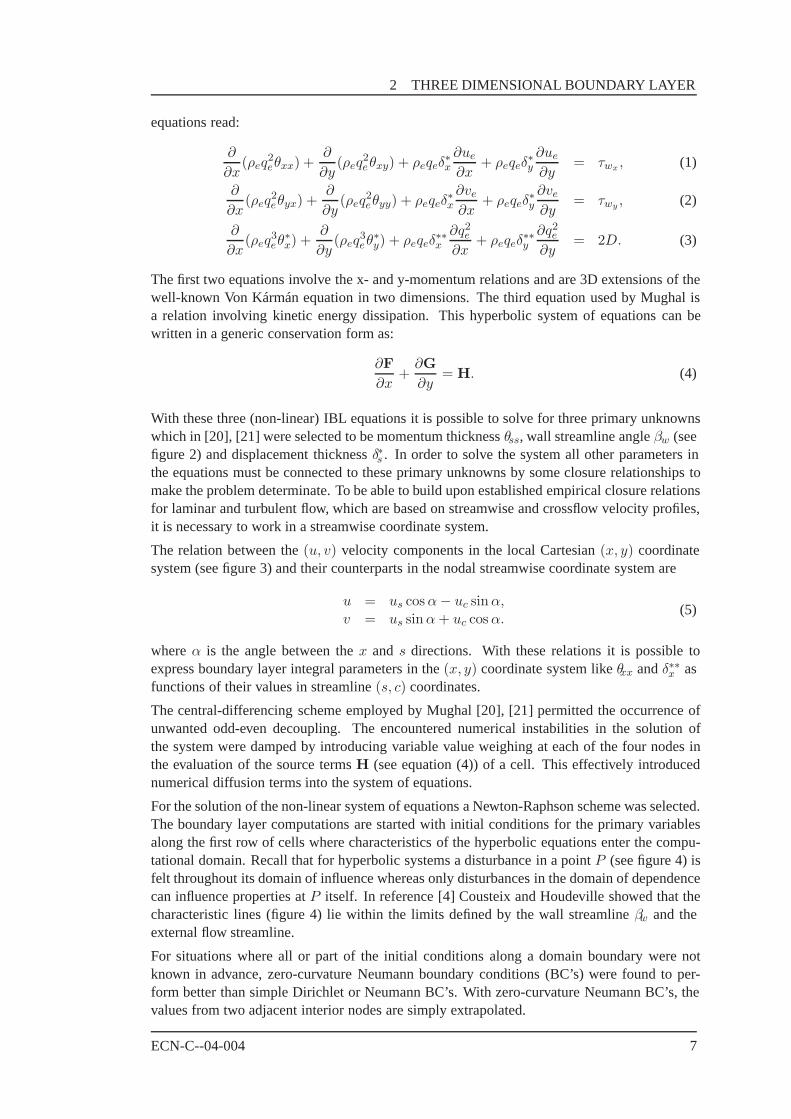
The first two equations involve the x- and y-momentum relations and are 3D extensions of thewell-known Von Kármán equation in two dimensions. The third equation used by Mughal isa relation involving kinetic energy dissipation. This hyperbolic system of equations can bewritten in a generic conservation form as:

∂F∂x

+∂G∂y

= H. (4)

With these three (non-linear) IBL equations it is possible to solve for three primary unknownswhich in [20], [21] were selected to be momentum thickness θss, wall streamline angle βw (seefigure 2) and displacement thickness δ∗s . In order to solve the system all other parameters inthe equations must be connected to these primary unknowns by some closure relationships tomake the problem determinate. To be able to build upon established empirical closure relationsfor laminar and turbulent flow, which are based on streamwise and crossflow velocity profiles,it is necessary to work in a streamwise coordinate system.

The relation between the (u, v) velocity components in the local Cartesian (x, y) coordinatesystem (see figure 3) and their counterparts in the nodal streamwise coordinate system are

u = us cos α − uc sin α,v = us sin α + uc cos α.

(5)

where α is the angle between the x and s directions. With these relations it is possible toexpress boundary layer integral parameters in the (x, y) coordinate system like θxx and δ∗∗x asfunctions of their values in streamline (s, c) coordinates.

The central-differencing scheme employed by Mughal [20], [21] permitted the occurrence ofunwanted odd-even decoupling. The encountered numerical instabilities in the solution ofthe system were damped by introducing variable value weighing at each of the four nodes inthe evaluation of the source terms H (see equation (4)) of a cell. This effectively introducednumerical diffusion terms into the system of equations.

For the solution of the non-linear system of equations a Newton-Raphson scheme was selected.The boundary layer computations are started with initial conditions for the primary variablesalong the first row of cells where characteristics of the hyperbolic equations enter the compu-tational domain. Recall that for hyperbolic systems a disturbance in a point P (see figure 4) isfelt throughout its domain of influence whereas only disturbances in the domain of dependencecan influence properties at P itself. In reference [4] Cousteix and Houdeville showed that thecharacteristic lines (figure 4) lie within the limits defined by the wall streamline βw and theexternal flow streamline.

For situations where all or part of the initial conditions along a domain boundary were notknown in advance, zero-curvature Neumann boundary conditions (BC’s) were found to per-form better than simple Dirichlet or Neumann BC’s. With zero-curvature Neumann BC’s, thevalues from two adjacent interior nodes are simply extrapolated.

ECN-C--04-004 7


xxxxxx

Domain ofDomain ofDependence

InfluenceP

Figure 4: Hyperbolic equation domains of dependence and influence.

In his conclusions Mughal [20] recommends to replace the ad hoc source-term weighing ap-proach by an upwind based discretization scheme. Further suggestions made are, the inclusionof the method in a viscous-inviscid interaction code, the addition of a more accurate model fornon-equilibrium boundary layers and the extension of the method to laminar flows with theassociated need for laminar-turbulent transition modeling. Very short computer CPU times of15 seconds are reported in reference [22] for a swept wing test case with 112 chordwise and22 spanwise grid cells. However, the results exhibit some spanwise oscillations.

Nishida, 1996

Nishida [24], [25] extended the original system of equations used by Mughal with an extraturbulent shear stress lag equation as derived by Green, Weeks and Brooman [9]:

δ

Cτ

∂Cτ

∂ξ= Kc

(C

12τeq − C

12τ

). (6)

The shear stress direction ξ was approximated and set to be the chordwise direction. The fourselected independent boundary layer variables were the shear stress coefficient factor C

1/2τ ,

the momentum thickness θss and the two displacement thicknesses δ∗s and δ∗c . The systemof equations was discretized using a weighed residual Petrov-Galerkin finite element method(FEM). In this approach the upwind-biased weight function, different from the shape function,provided for a stable discretization scheme. For a description of FEM discretization solutionsused in CFD codes the reader is referred to reference [10] and [11]. The IBL equations werecoupled in full simultaneous interaction with a full-potential solver for the external flow. ANewton-Raphson method was applied for the combined solution of the non-linear equationsfor the external flow and the boundary layer region.

Boundary layer computations are started with initial conditions specified for the primary vari-ables along the attachment line. Zero-curvature Neumann BC’s applied in a test case wherenot all initial conditions along a domain boundary were known in advance, were shown to giveanomalous results. Nishida states that the correct BC’s should specify all incoming charac-teristic variables. However, this was considered too difficult to implement and a modified BCwas constructed in which one of the primary variables was allowed to float, Nishida chose thecrossflow displacement thickness δ∗c , while all others were explicitly specified.

An additional set of BL parameter closure relationships was included to enable the simula-tion of laminar boundary layers. Laminar-turbulent transition was assumed to occur at pre-determined chordwise locations. The effect of boundary layer displacement thickness on theexternal flow was accounted for by a surface normal transpiration velocity.

Impressive results for separated transonic flow about a swept wing were shown in reference[24]. However, some difficulties with the robustness of the code were reported that could be

8 ECN-C--04-004


attributed to the specific handling of the kinetic energy equation (3). The fully simultaneouscoupling scheme for the viscous and inviscid flow regions was found to put large demandsupon computer CPU time and memory allocation.

Milewski, 1997

Milewski’s work in reference [19] was based on Nishida’s formulation with the essential dif-ference being the handling of the external flow by a first order accurate panel method insteadof a full-potential code. An explicit numerical dissipation term was added to the x- and y-momentum IBL equations (1) and (2) to prevent spanwise oscillations in the solution thatoccurred in cases with coarse spanwise grid resolution. For a swept wing test case good agree-ment with experiment was found for the overal lift force, even in 3D separated flow. Computedpressure distributions for a circular duct were compared with experimental data and, apartfrom some discrepancies at the trailing edge, found to be in good agreement. Drag forces weregenerally underpredicted.

In his recommendations, Milewski mentions the large computational requirements that resultfrom the assembly and inversion of the Jacobian matrix used in the Newton-Raphson scheme.Another suggestion made is to examine in more detail the finite trailing edge loading that wasbelieved to be caused by the algorithm used to compute the external velocities at the trailingedge nodes.

Mughal, 1998

A more fundamental study of the mathematical aspects of 3D integral boundary layer approx-imations was reported in the PhD. thesis of Mughal [22]. The derivation of all relevant IBLequations was based on the differential form of the boundary layer equations for conservationof mass and x- and y-momentum:

∂ρ

∂t+ ∇ · (ρu) = 0, (7)

ρ∂u

∂t+ ρu · ∇u +

∂p

∂x=

∂τx

∂z, τx = µ

∂u

∂z− ρu′w′, (8)

ρ∂v

∂t+ ρu · ∇v +

∂p

∂y=

∂τy

∂z, τy = µ

∂v

∂z− ρv′w′. (9)

The time dependent version of any set of IBL equations was written in a generic conservationform (see also equation (4)) as:

∂U∂t

+∂F∂x

+∂G∂y

= H. (10)

In this equation U is the solution vector, F and G are flux vectors and H is a source vector.It is mentioned here that all results shown by Mughal in reference [22] were actually based onthe steady form of the BL equations.

A number of streamwise and crossflow velocity profile families for laminar and turbulent flowwere considered. Normally these velocity profiles are used to derive some explicit closurerelationships between boundary layer parameters. However, Mughal computed the closure re-lations on the fly from the assumed set of BL velocity profiles. This gives greater flexibility forthe choice of streamwise and crossflow velocity profile families. A drawback of this approachis the loss of direct control of the closure functions. Based on the nature of the unsteady dif-ferential form of the BL equations, a justification for the requirement for hyperbolicity of the

ECN-C--04-004 9


complete resulting IBL sytem was given (i.e. BL equations plus closure relations). It should bementioned that only for some simple closure functions the hyperbolic character of the IBL sys-tem can be proven. In practice, hyperbolicity of the system is assumed. A method to enforcehyperbolicity by constraining the closure relationships was devised but discarded for actualimplementation. Several strategies for the solution of the system of steady and unsteady IBLequations were suggested. The Petrov-Galerkin FEM method from Nishida (references [24]and [25]) was enhanced with a more sophisticated upwinding based weight function. In orderto be able to compute bi-directional crossflows (see figure 5) the system of momentum equa-tions and total kinetic energy equation was extended with a mixed velocity component kineticenergy equation.

uc

c

n

Figure 5: Uni-directional and bi-directional crossflow velocity profiles uc .

A demonstration computer program was constructed, employing a fully simultaneous couplingof the steady 3D IBL equation model and a first order accurate panel method for the externalflow. The method, flexible in the choice of applied velocity profiles, was demonstrated to beable to compute 3D separated flows. For the theory of panel methods, also known as boundaryelement methods or linear potential flow solvers, the interested reader is referred to references[12], [13] and [14].

In the conclusions of reference [22], Mughal recommends to refine and implement the schemeto enforce hyperbolicity of the combined system of IBL equations and closure functions. Fur-ther suggestions made are the implementation of laminar-turbulent transition criteria and thereplacement of the CPU-intensive direct matrix inversion method by an iterative solver in con-junction with a sparse matrix approximation for the full residual Jacobian matrix. In addition,to simplify the data structure for the BL parameters, it is proposed to integrate the differentialBL equations themselves numerically on the fly. The rotation of BL thicknesses can then beimplemented by just decomposing the velocity vectors in streamwise and crossflow direction.

Coenen, 2000

The main topic of the work by Coenen [1] was the interaction scheme for the coupling of theexternal flow model and an IBL method for the viscous flow region. In the 3D IBL method thekinetic energy integral equation (3) was replaced by an entrainment equation:

1qe

∂

∂x(ueδ − qeδ

∗x) +

1qe

∂

∂y(veδ − qeδ

∗y) = CE. (11)

For the solution of this system of equations the momentum thickness θss, the shape factorH (where H = δ∗s/θss), and the limiting wall streamline angle βw were selected to be the

10 ECN-C--04-004


independent variables. The hyperbolic nature of the IBL equations was taken into accountby the use of upwind discretizations for the derivative terms in the cell-vertex FVM. Alongthe attachment line initial conditions are specified for the primary variables. Symmetry BC’swere applied at the wing root section and for the tip section the variables were determined byextrapolation of values at interior nodes.

For the laminar part of the boundary layer a very simple 2D integral method was used. Theposition of natural transition to turbulent flow was predicted with a simple empirical criterionand the effect of a possible laminar separation bubble on starting conditions for the turbulentboundary layer was taken into account. The IBL equations were coupled, with the quasi-simultaneous interaction algorithm by Veldman [38], to a first order accurate panel methodfor the external flow. The coupled system of boundary layer, external flow and interactionequations was solved using a Newton-Raphson method. For some 3D wing aerodynamics testcases the pressure distributions and boundary layer parameters were found to be in reasonableagreement with experimental data. Some discrepancies were noticed in the trailing edge regionthat were attributed to the inaccurate modeling of the Kutta condition in the panel method.For an overview of viscous-inviscid interaction techniques the interested reader is referred toreference [17].

2.3 Rotation and Time Dependency

The momentum equations so far are formulated for an inertial coordinate system. For a steadilyrotating frame of reference two force vector terms have to be added to H in the right hand sideof equation (10). The first is the Coriolis force term

ρf1 = −2ρ(Ω × u), (12)

and the second is a centrifugal force term:

ρf2 = −ρΩ × (Ω × r). (13)

When incompressible flow is assumed and the rotation associated velocity component u =Ω × r is incorporated in the pressure formula, the centrifugal force term does not have toappear explicitly in the momentum equations (see [30]).

For an arbitrarily translating and rotating frame of reference two more force vectors are in-troduced in the momentum equations. Due to the time dependency of the translation velocity∂ X/∂t, a force term is introduced:

ρf3 = −ρ∂2 X

∂t2, (14)

and the time dependency of the angular velocity gives rise to another force vector:

ρf4 = −ρ∂Ω∂t

× r. (15)

In compressible flow all four force terms will appear in the source term H of equation (10) andwill merely add inhomogeneities to the problem. No additional discretization difficulties areexpected in the implementation of these terms.

Wind turbine rotor blades generally operate in low frequency periodic flows with small char-acteristic Strouhal numbers

St = Lref/(tref qref ).

ECN-C--04-004 11


As a result, the flow can be considered to be quasi-steady: at any point in time the solutionbehaves as the corresponding steady solution with the instantaneous outer flow (see [27]). Thismeans that periodicity effects on the assumed set of BL velocity profiles can be neglected.

In flutter conditions with small amplitude, high frequency oscillations, the flow cannot be con-sidered quasi-steady and unsteady flow effects should be reflected in the assumed set of BLvelocity profiles. A possible approach is to combine the basis set of velocity profiles with avelocity profile family typical for oscilating boundaries. In figure 6 such a profile family isshown: Stokes’ steady state solution (see [27]) for BL flow near an in-plane oscillating wallwith velocity uw = sin T .

0

1

2

3

4

5

-1 -0.5 0 0.5 1

T = 0.00πT = 0.25πT = 0.50πT = 0.75πT = 1.00πT = 1.25πT = 1.50πT = 1.75πT = 2.00π

u

n

Figure 6: Stokes’ steady state solution for flow near an in-plane oscillating plate.

A crucial step towards solving the set of time-dependent IBL equations (see the system ofequations (10)), is to recognize that the spatially discretized problem represents a non-linearsystem of ordinary differential equations. As was mentioned by Mughal [22], the solutionof this unsteady IBL system can be accomplished by integrating the equations in time. Forthe discretization a multitude of options are available with differences in accuracy, stability,robustness, efficiency and complexity. Many of the schemes can be found in textbooks like[8], [10], [11] and [43]. A discussion of these numerical algorithms is outside the scope of thisproject.

Swafford [33] and Swafford and Whitfield [35] derived the unsteady form of the momentumand kinetic energy IBL equations for compressible flow in a non-orthogonal curvilinear co-ordinate system. The unsteady IBL equations were used to obtain solutions for steady flowproblems. Two- and four-stage explicit Runge-Kutta time-stepping schemes were used for in-tegration in time. Local time steps were used to accelerate convergence to steady state. For thespatial discretization an upwind scheme was found to give the best results.

The differential form of the unsteady IBL equations was used by Van der Wees and VanMuijden [42] in strong interaction with a full-potential flow solver. They stated that an im-portant advantage of using the unsteady boundary layer equations for solving steady boundarylayer flow is the robustness of such an approach. For the time integration scheme a fully im-plicit backward Euler method was selected. In later reports the code was demonstrated for testcases with mildly separated flow. For the VII scheme the steady form of the quasi-simultaneousinteraction algorithm was used.

The unsteady version of the quasi-simultaneous VII scheme was found by Coenen [1] to lead

12 ECN-C--04-004


to a better conditioned interaction problem than its steady counterpart. This conclusion waspositively confirmed by Veldman [40].

ECN-C--04-004 13

14 ECN-C--04-004

3 CLOSURE RELATIONS

3.1 Introduction

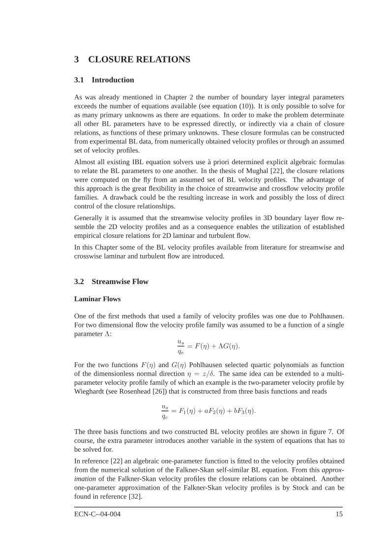
As was already mentioned in Chapter 2 the number of boundary layer integral parametersexceeds the number of equations available (see equation (10)). It is only possible to solve foras many primary unknowns as there are equations. In order to make the problem determinateall other BL parameters have to be expressed directly, or indirectly via a chain of closurerelations, as functions of these primary unknowns. These closure formulas can be constructedfrom experimental BL data, from numerically obtained velocity profiles or through an assumedset of velocity profiles.

Almost all existing IBL equation solvers use à priori determined explicit algebraic formulasto relate the BL parameters to one another. In the thesis of Mughal [22], the closure relationswere computed on the fly from an assumed set of BL velocity profiles. The advantage ofthis approach is the great flexibility in the choice of streamwise and crossflow velocity profilefamilies. A drawback could be the resulting increase in work and possibly the loss of directcontrol of the closure relationships.

Generally it is assumed that the streamwise velocity profiles in 3D boundary layer flow re-semble the 2D velocity profiles and as a consequence enables the utilization of establishedempirical closure relations for 2D laminar and turbulent flow.

In this Chapter some of the BL velocity profiles available from literature for streamwise andcrosswise laminar and turbulent flow are introduced.

3.2 Streamwise Flow

Laminar Flows

One of the first methods that used a family of velocity profiles was one due to Pohlhausen.For two dimensional flow the velocity profile family was assumed to be a function of a singleparameter Λ:

us

qe= F (η) + ΛG(η).

For the two functions F (η) and G(η) Pohlhausen selected quartic polynomials as functionof the dimensionless normal direction η = z/δ. The same idea can be extended to a multi-parameter velocity profile family of which an example is the two-parameter velocity profile byWieghardt (see Rosenhead [26]) that is constructed from three basis functions and reads

us

qe= F1(η) + aF2(η) + bF3(η).

The three basis functions and two constructed BL velocity profiles are shown in figure 7. Ofcourse, the extra parameter introduces another variable in the system of equations that has tobe solved for.

In reference [22] an algebraic one-parameter function is fitted to the velocity profiles obtainedfrom the numerical solution of the Falkner-Skan self-similar BL equation. From this approx-imation of the Falkner-Skan velocity profiles the closure relations can be obtained. Anotherone-parameter approximation of the Falkner-Skan velocity profiles is by Stock and can befound in reference [32].

ECN-C--04-004 15


0

0.2

0.4

0.6

0.8

1

-0.4 -0.2 0 0.2 0.4 0.6 0.8 1

F12F2

10F3

η

Us/Ue

Figure 7: Wieghardt’s streamwise velocity functions [26].

Of course the closure relationships could also have been constructed from the numerical re-sults of the Falkner-Skan equation directly. In his thesis Drela [6] obtained a number of one-parameter curve fits that way.

Turbulent Flows

For turbulent flows exact numerical solutions to the BL equations are not possible. Veloc-ity profiles for turbulent boundary layers therefore have been constructed with the help ofexperimental data. Multiple layers can be distinguished in a turbulent velocity profile and aone-parameter velocity profile family is inadequate to describe all turbulent boundary layers.

Noticeable two-parameter models for complete turbulent velocity profiles, able to representseparated flow, are due to Swafford [34] and Cross [5] which respectively take the form

us

qe=

s

0.09u+e

arctan(0.09y+) +(

1 − sπ

0.18u+e

) √tanh(aηb),

andus

qe=

uτ cos βw

κ

(12

ln(Rδuτη)2 + A

)+ Bs sinχs

(π

2η

).

As was mentioned in the introduction of this chapter, except for Mughal [22], the velocity pro-file models are almost exclusively used to obtain algebraic closure relations. Closure relationsthat were derived from Swafford’s model were used by Drela [6], Mughal [20], Nishida [24]and Milewski [19].

3.3 Crossflow

Laminar Flows

As in Pohlhausen’s approximation of streamwise laminar profiles it is possible to construct one-or multi-parameter velocity profiles for crosswise flow. In reference [32], Stock constructeda two-parameter crossflow velocity profile family allowing for bidirectional crossflows. Thespecific form of the two basis functions G1 and G2, shown in figure 8, was established with thehelp of results from a 3D differential BL solver. In the same figure some resulting crossflowvelocity profiles uc = cG1(η) + dG2(η) are shown.

16 ECN-C--04-004

3 CLOSURE RELATIONS

0

0.2

0.4

0.6

0.8

1

-2.5 -2 -1.5 -1 -0.5 0 0.5 1 1.5 2 2.5

50G1G2

η

Uc/Ue

Figure 8: Stock’s crossflow velocity functions [32] .

A two-parameter model taken from reference [22] uses the streamwise velocity profile in itsdefinition:

uc

qe= (1 − us

qe)(cη + dη2).

To solve for the second unknown parameter an extra equation is required. In reference [22]Mughal examined a system of equations and obtained results comparable with those from adifferential type of BL solver for a laminar flow problem with the crosswise pressure gradientalternating along the streamlines.

Turbulent Flows

A common approach in modeling crossflow velocity profiles is to base them on the scaling ofthe streamwise velocity profile. Two frequently used models are due to Johnston and Mager.The model of Johnston, used by Mughal [20], Nishida [24] and Swafford [34], reads:

uc

qe=

usqe

tan βw η ≤ η∗,c(1 − us

q ) η > η∗.

Mager’s model was used by Coenen in reference [1]. The model uses a simple parabolic scalingfunction and is expressed as

uc

qe=

us

qe(1 − η)2 tan βw.

In reference [36] Tai suggested a modification of Mager’s function that prevents the unrealisticincrease in velocity magnitude in the combined velocity profile at large crossflow angles.

A model for the complete crossflow velocity profile was defined in reference [5] by Cross. Itsuse was recommended by Coenen [1] over Mager’s model which was established for fairlysmall limiting crossflow angles βw.

uc

qe=

uτ sin βw

κ

(12

ln(Rδuτη)2 + A

)+ Bc sinχc

(π

2η

).

ECN-C--04-004 17

18 ECN-C--04-004

4 CONCLUSIONS AND RECOMMENDATIONS

In this report the feasibility of a rotor aerodynamics simulation code composed of a “panelmethod” solver for the external flow and an integral boundary layer method for the viscousflow regions is shown through a discussion of existing succesfull integral boundary layer ap-proaches and the impact of time-dependency and rotor blade rotation related terms on the sys-tem of equations. As a result, the development of the targeted wind turbine rotor aerodynamicssimulation code is recommended.

Some detailed conclusions and recommendations are given below.

4.1 Conclusions

A concise survey is given of the available theories and solution approaches for integral bound-ary layer methods that have proven themselves in practical computations of separated flows.(see [1], [19], [20], [21], [22], [24], [25], [42]).

The viability of an aerodynamic simulation model employing the unsteady quasi-simultaneouscoupling of an IBL method for the viscous flow and a panel method for the inviscid externalflow was confirmed positively by Veldman [40].

The conservation form of the integral boundary layer equations was first employed by Mughalin reference [20] and [21]. The finite volume method that was used for the solution of theequations circumvents the explicit introduction of awkward metric coefficients and geodesiccurvature terms.

From the options to suppress instabilities and oscillations in the solution of the integral bound-ary layer equations the upwind discretization schemes are preferred over central schemes withexplicit numerical damping terms.

Time-dependent terms in the integral boundary layer equations and in the quasi-simultaneousinteraction scheme both enhance the robustness of the flow solver.

The fully simultaneous coupling scheme for the interaction between viscous and inviscid flowregions is expensive with regard to the allocation of computer resources.

For a steadily rotating frame of reference, Coriolis force and centrifugal force vectors must beadded to the source term of the momentum equations. In case of an arbitrarily translating androtating frame of reference two more force vectors should be included in addition.

Both Coenen [1] and Milewski [19] employed a panel method for the external flow about winggeometries and reported difficulties in the interaction with the boundary layer solver at thetrailing edge. The problem was attributed to the pressure difference across the trailing edge ascomputed by the panel method.

Most of the existing integral boundary layer solvers use à priori determined explicit algebraicclosure relations to render the system of equations determinate. An exception is the approachtaken by Mughal [22] where the closure relations were computed on the fly from an assumedset of boundary layer velocity profiles.

In reference [22] a method was devised to enforce hyperbolicity of the system of boundarylayer equations by constraining the closure relationships. It was recommended to refine thescheme and implement it in the integral boundary layer solver.

Laminar-turbulent transition modeling is a topic that received very little attention in the re-viewed reports.

For the temporal and spatial discretization of hyperbolic unsteady integral boundary layer equa-

ECN-C--04-004 19


tions with finite volume or finite element methods a vast amount of schemes is available eachwith its own characteristics regarding accuracy, stability, robustness, efficiency and complexity.This vastness of options poses a problem for the selection of the “right” discretization schemes.

4.2 Recommendations

For the development of an integral boundary layer solver, to be coupled in strong interactionwith a panel method for the external flow, some recommendations can be given:

• Employ a Finite Volume Method or a Finite Element Method to solve the conservationform of the time-dependent integral boundary layer equations.

• The vast amount of available solution strategies for the time-dependent integral bound-ary layer equations strongly suggests to do code development in close cooperation withexperts in the field of computational fluid dynamics.

• Separated flow about wind turbine rotor blades exhibit large crossflow components. Thissuggests the use of an advanced model for the turbulent crossflow velocity profile familylike the model by Cross [5].

• In order to avoid problems with the viscous-inviscid interaction scheme at the trailingedge, the implementation of a zero pressure difference Kutta condition in the panelmethod is recommended.

• If a coupling of the integral boundary layer solver with a compressible flow solver isanticipated, the compressible form of the boundary layer equations should be used.

• Laminar-turbulent transition modeling is a topic that should be part of the developmentof an integral boundary layer solver.

• Mughal [22] integrated the boundary layer velocity profiles on the fly, avoiding the needfor explicit boundary layer closure functions. In addition, a recommendation was tointegrate the differential equations over the boundary layer thickness in the course of thesimulation. Both ideas are worth investigating.

20 ECN-C--04-004

REFERENCES

[1] E.G.M. Coenen, Viscous-Inviscid Interaction Method for 2D and 3D Aerodynamic Flow,PhD. Thesis, Rijksuniversiteit Groningen, 2001

[2] J. Cousteix, Theoretical Analysis and Prediction Means of a Three-Dimensional Turbu-lent Boundary Layer, ONERA Publication No. 157 (in French), 1974

[3] J. Cousteix, Three-Dimensional Boundary Layers. Introduction to Calculation Methods,AGARD R-741, paper 1, pp.1-48, 1986

[4] J. Cousteix, R. Houdeville, Singularities in Three-Dimensional Turbulent BoundaryLayer Calculations and Separation Phenomena, AIAA J., Vol.19, No.8, pp.976-985,1981

[5] A.G.T. Cross, Boundary Layer Calculation and Viscous-Inviscid Coupling, ICAS-86-2.4.1, 1986

[6] M. Drela, Two-Dimensional Transonic Aerodynamic Design and Analysis using the EulerEquations, PhD. Thesis, Massachusetts Institute of Technology, 1985

[7] M. Drela, XFOIL: An Analysis and Design System for Low Reynolds Number Airfoils,in “Conference on Low Reynolds Number Aerodynamics”, University of Notre Dame,1989

[8] J.H. Ferziger, M. Peric, Computational Methods for Fluid Dynamics Springer, 1996

[9] J.E. Green, D.J. Weeks, J.W.F. Brooman, Prediction of Turbulent Boundary Layers andWakes in Compressible Flow by a Lag-Entrainment Method, R&M 3791, R.A.E., 1973

[10] C. Hirsch, Numerical Computation of Internal and External Flows. Volume 1. Funda-mentals of Numerical Discretization, John Wiley & Sons, 1992

[11] C. Hirsch, Numerical Computation of Internal and External Flows. Volume 2. Computa-tional Methods for Inviscid and Viscous Flows, John Wiley & Sons, 1992

[12] H.W.M. Hoeijmakers, Panel Methods for Aerodynamic Analysis and Design, In:AGARD-FDP/VKI Special Course on Engineering Methods in Aerodynamic Analysisand Design of Aircraft, AGARD Report R-783, NLR TP 91404 L, 1991.

[13] B. Hunt, The Panel Method for Subsonic Aerodynamic Flows: A Survey of Mathemat-ical Formulations and Numerical Models and an Outline of the New British AerospaceScheme, VKI Lecture Series 1978-4, 1978.

[14] J. Katz, A. Plotkin, Low-Speed Aerodynamics: From Wing Theory to Panel Methods,McGraw-Hill, 1991.

[15] J.C. Le Balleur, Numerical Viscous-Inviscid Interaction in Steady and Unsteady Flows,Numerical and Physical Aspects of Aerodynamic Flows II, Ch.13, 1984.

[16] J.C. Le Balleur, New Possibilities of Viscous-Inviscid Numerical Techniques for SolvingViscous Flow Equations with Massive Separation, ONERA TP-1989-24, 1989

[17] R.C. Lock, B.R. Williams, Viscous-Inviscid Interaction in External Aerodynamics, Prog.Aerospace Sci., Vol.24, pp.51-171, 1987

ECN-C--04-004 21


[18] A. Mager, Generalization of Boundary-Layer Momentum-Integral Equations to Three-Dimensional Flows Including those of Rotating Systems, NACA TR 1067, 1952

[19] W.M. Milewski, Three-Dimensional Viscous Flow Computations Using the BoundaryLayer Equations Simultaneously Coupled with a Low Order Panels Method, PhD. Thesis,Massachusetts Institute of Technology, 1997

[20] B. Mughal, A Calculation Method for the Three-Dimensional Boundary-Layer Equationsin Integral Form, MSc. Thesis, Massachusetts Institute of Technology, 1992

[21] B. Mughal, M. Drela, A Calculation Method for the Three-Dimensional Boundary-LayerEquations in Integral Form, AIAA 93-0786, 1993

[22] B. Mughal, Integral Methods for Three-Dimensional Boundary-Layers, PhD. Thesis,Massachusetts Institute of Technology, 1998

[23] D.F. Myring, An Integral Prediction Method for Threedimensional Turbulent BoundaryLayers in Incompressible Flow, Technical Report 70147, Royal Aircraft Establishment,1970

[24] B.A. Nishida, Fully Simultaneous Coupling of the Full Potential Equation and the Inte-gral Boundary Layer Equations in Three Dimensions, PhD. Thesis, Massachusetts Insti-tute of Technology, 1996

[25] B. Nishida, M. Drela, Fully Simultaneous Coupling for Three-Dimensional Vis-cous/Inviscid Flows, AIAA 95-1806, 1995

[26] L. Rosenhead, Laminar Boundary Layers, Oxford University Press, 1963

[27] H. Schlichting, K. Gersten, Boundary Layer Theory, Springer, 2000

[28] P.D. Smith, An Integral Prediction Method for Three-Dimensional Compressible Turbu-lent Boundary Layers, Aeronautical Research Council, R&M 3739, 1974

[29] H. Snel, R. Houwink, J. Bosschers, Sectional Prediction of Lift Coefficients on RotatingWind Turbine Blades in Stall, ECN-C--93-052, 1994

[30] J.N. Sørensen, Prediction of Three-Dimensional Stall on Wind Turbine Blade usingThree-Level, Viscous-Inviscid Interaction Model, EWEC ’86, European Wind Energy As-sociation Conference and Exhibition, pp.429-435, 1986

[31] H.W. Stock, Integral Method for the Calulation of Three-Dimensional, Laminar and Tur-bulent Boundary Layers, NASA TM 75320, 1978

[32] H.W. Stock, H.P. Horton, Ein Integralverfahren zur Berechnung dreidimensionaler, lam-inarer, kompressibler, adiabater Grenzschichten, Z. Flugwiss. Weltraumforsch. 9 (1985),Heft 2, pp.101-110

[33] T.W. Swafford, Three dimensional, Time-Dependent, Compressible, Turbulent, IntegralBoundary-Layer Equations in General Curvilinear Coordinates and Their Numerical So-lution, PhD. Thesis, Mississippi State University, 1983.

[34] Swafford, T.W. , Analytical approximation of two-dimensional separated turbulentboundary-layer velocity profiles, AIAA Journal, Vol.21, No.6, pp.923-926, 1983.

22 ECN-C--04-004

REFERENCES

[35] T.W. Swafford, D.L. Whitfield, Time-Dependent Solution of Three-Dimensional Com-pressible Turbulent Integral Boundary-Layer Equations, AIAA J., Vol.23, No.7, pp.1005-1013, 1985

[36] T.C. Tai, An Integral Method for Three-Dimensional Turbulent Boundary Layer withLarge Crossflow, AIAA-87-1254, 1987

[37] B. Thwaites, Approximate Calculation of the Laminar Boundary Layer, The Aeron.Quart., Vol.1, pp.245-280, 1949

[38] A.E.P. Veldman, The Calculation of Incompressible Boundary Layers with StrongViscous-Inviscid Interaction, AGARD CP-291, paper 12, 1980

[39] A.E.P. Veldman, New, Quasi-Simultaneous Method to Calculate Interacting BoundaryLayers, AIAA J., Vol.19, pp.79-85, 1981

[40] A.E.P. Veldman, Personal communication, 2003

[41] Z.U.A. Warsi, Fluid Dynamics, Theoretical and Computational Approaches, CRC Press,1998

[42] A.J. van der Wees, J. van Muijden, A Robust Quasi-Simultaneous Interaction Method fora Full Potential Flow with a Boundary Layer with Application to Wing/Body Configu-rations, In “Proc. 5th Symp. on Num. and Phys. Aspects of Aerodynamic Flows”, LongBeach, California, U.S.A., January 13-15, 1992

[43] P. Wesseling, Principles of Computational Fluid Dynamics, Springer, 2001

[44] B.A. Wolles, Computational Viscid-Inviscid Interaction Modelling of the Flow aboutAerofoils, PhD. Thesis, University of Twente, 1999

ECN-C--04-004 23


24 ECN-C--04-004

Date: December 2003 Number of report: ECN-C--04-004Title INTEGRAL BOUNDARY LAYER METHODS FOR

WIND TURBINE AERODYNAMICSSubtitle A Literature SurveyAuthor(s) A. van GarrelPrincipal(s) Novem BV.ECN project number 7.4188Principal(s) project number 2020-02-13-20-008Programme(s) BSE DEN 2002AbstractThe simulation of wind turbine rotor aerodynamics can be improved upon by increasing thephysics content in the underlying approximations. The current effort is targeted at an aerody-namics model in which the flow field is decomposed into two domains. The inviscid externalflow domain is modeled with a “panel method” type of flow solver and the viscous regions aremodeled with an integral boundary layer model. For the simulation of separated flows the twomodels are coupled in strong interaction. The technology for the “panel method” flow solveris considered common knowledge and is not expected to raise serious problems during its de-velopment. In this report the possibilities and difficulties in the development of the integralboundary layer solver are investigated. The feasibility of the development of the rotor aero-dynamics simulation code is shown through a discussion of succesful integral boundary layerapproaches based on the conservation form of the boundary layer equations and the impact oftime-dependency and rotor blade rotation related terms on the system of equations. In additiona number of possible boundary layer velocity profiles is described. As a result the developmentof the targeted wind turbine rotor aerodynamics simulation code is recommended. Due to thevast amount of possible solution strategies it is advised to develop the boundary layer solver inclose cooperation with experts in the field of computational fluid dynamics.

Keywords wind turbines, aerodynamics, boundary layers, viscous-inviscidinteraction

Authorization Name Signature DateChecked D. WinkelaarApproved H. SnelAuthorized H.J.M. Beurskens

integral boundary layer methods for wind turbine aerodynamics · integral boundary layer methods...

Documents