instruments and controls - website cá nhân giáo viêns standard... · instruments and controls...
TRANSCRIPT
Section 16Instruments and Controls
BY
O. MULLER-GIRARD Consulting Engineer, RochesGREGORY V. MURPHY Process Control ConsultanW. DAVID TETER Professor, Department of Civil E
University of Delaware.
Counting Events . . . . . . . . . . . . . . . . . . . . . . . . . . . . . . . . .Time and Frequency Measurement . . . . . . . . . . . . . . . . . .Mass and Weight Measurement . . . . . . . . . . . . . . . . . . . . .Measurement of Linear and Angular Displacement . . . . .Measurement of Area . . . . . . . . . . . . . . . . . . . . . . . . . . . . .Measurement of Fluid Volume . . . . . . . . . . . . . . . . . . . . .Force and Torque Measurement . . . . . . . . . . . . . . . . . . . . . .
Copyright (C) 1999 by The McGraw-Hill Companies, Inc. All rights reserved. Use ofthis product is subject to the terms of its License Agreement. Click here to view.
ter, NY.t, DuPont Co.ngineering, College of Engineering,
lements . . . . . . . . . . . . . . . . . . . . . . . . . . . . . . . . . . . . . . . . . 16-30
16.1 INSTRUMENTSby Otto Muller-Girard
Introduction to Measurement . . . . . . . . . . . . . . . . . . . . . . . . . . . . . . . . . . . . . 16-2 Final Control E
. . . . . . . . . . . . . . 16-2. . . . . . . . . . . . . . 16-3. . . . . . . . . . . . . . 16-3. . . . . . . . . . . . . . 16-4. . . . . . . . . . . . . . 16-7. . . . . . . . . . . . . . 16-7. . . . . . . . . . . . . 16-7Hydraulic-Control Systems . . . . . . . . . . . . . . . . . . . . . . . . . . . . . . . . . . . . . 16-30Steady-State Performance . . . . . . . . . . . . . . . . . . . . . . . . . . . . . . . . . . . . . . 16-32Closed-Loop Block Diagram . . . . . . . . . . . . . . . . . . . . . . . . . . . . . . . . . . . . 16-32Frequency Response . . . . . . . . . . . . . . . . . . . . . . . . . . . . . . . . . . . . . . . . . . . 16-33Graphical Display of Frequency Response . . . . . . . . . . . . . . . . . . . . . . . . . 16-34Nyquist Plot . . . . . . . . . . . . . . . . . . . . . . . . . . . . . . . . . . . . . . . . . . . . . . . . . 16-34Bode Diagram . . . . . . . . . . . . . . . . . . . . . . . . . . . . . . . . . . . . . . . . . . . . . . . . 16-34Controllers on the Bode Plot . . . . . . . . . . . . . . . . . . . . . . . . . . . . . . . . . . . . 16-37Stability and Performance of an Automatic Control . . . . . . . . . . . . . . . . . . 16-37
Pressure and Vacuum Measurement . . . . . . . . . . . . . . . . . . . . . . . . . . . . . . . 16-8Liquid-Level Measurement . . . . . . . . . . . . . . . . . . . . . . . . . . . . . . . . . . . . . . 16-9Temperature Measurement . . . . . . . . . . . . . . . . . . . . . . . . . . . . . . . . . . . . . . . 16-9Measurement of Fluid Flow Rate . . . . . . . . . . . . . . . . . . . . . . . . . . . . . . . . . 16-13Power Measurement . . . . . . . . . . . . . . . . . . . . . . . . . . . . . . . . . . . . . . . . . . . 16-15Electrical Measurements . . . . . . . . . . . . . . . . . . . . . . . . . . . . . . . . . . . . . . . 16-16Velocity and Acceleration Measurement . . . . . . . . . . . . . . . . . . . . . . . . . . . 16-17Measurement of Physical and Chemical Properties . . . . . . . . . . . . . . . . . . . 16-18Nuclear Radiation Instruments . . . . . . . . . . . . . . . . . . . . . . . . . . . . . . . . . . . 16-19Indicating, Recording, and Logging . . . . . . . . . . . . . . . . . . . . . . . . . . . . . . . 16-19Information Transmission . . . . . . . . . . . . . . . . . . . . . . . . . . . . . . . . . . . . . . 16-20
16.2 AUTOMATIC CONTROLSby Gregory V. Murphy
Introduction . . . . . . . . . . . . . . . . . . . . . . . . . . . . . . . . . . . . . . . . . . . . . . . . . 16-22Basic Automatic-Control System . . . . . . . . . . . . . . . . . . . . . . . . . . . . . . . . . 16-22Process as Part of the System . . . . . . . . . . . . . . . . . . . . . . . . . . . . . . . . . . . . 16-23Transient Analysis of a Control System . . . . . . . . . . . . . . . . . . . . . . . . . . . 16-24Time Constants . . . . . . . . . . . . . . . . . . . . . . . . . . . . . . . . . . . . . . . . . . . . . . . 16-26Block Diagrams . . . . . . . . . . . . . . . . . . . . . . . . . . . . . . . . . . . . . . . . . . . . . . 16-27Signal-Flow Representation . . . . . . . . . . . . . . . . . . . . . . . . . . . . . . . . . . . . . 16-28Controller Mechanisms . . . . . . . . . . . . . . . . . . . . . . . . . . . . . . . . . . . . . . . . 16-28
Sampled-Data Control Systems . . . . . . . . . . . . . . . . . . . . . . . . . . . . . . . . . . 16-38Modern Control Techniques . . . . . . . . . . . . . . . . . . . . . . . . . . . . . . . . . . . . . 16-39Mathematics and Control Background . . . . . . . . . . . . . . . . . . . . . . . . . . . . . 16-41Evaluating Multivariable Performance and Stability Robustness of
a Control System Using Singular Values . . . . . . . . . . . . . . . . . . . . . . . . . 16-41Review of Optimal Control Theory . . . . . . . . . . . . . . . . . . . . . . . . . . . . . . . 16-43Procedure for LQG/LTR Compensator Design . . . . . . . . . . . . . . . . . . . . . . 16-44Example Controller Design for a Deaerator . . . . . . . . . . . . . . . . . . . . . . . . 16-45Analysis of Singular-Value Plots . . . . . . . . . . . . . . . . . . . . . . . . . . . . . . . . . 16-48Technology Review . . . . . . . . . . . . . . . . . . . . . . . . . . . . . . . . . . . . . . . . . . . 16-49
16.3 SURVEYINGby W. David Teter
Introduction . . . . . . . . . . . . . . . . . . . . . . . . . . . . . . . . . . . . . . . . . . . . . . . . . 16-50Horizontal Distance . . . . . . . . . . . . . . . . . . . . . . . . . . . . . . . . . . . . . . . . . . . 16-50Vertical Distance . . . . . . . . . . . . . . . . . . . . . . . . . . . . . . . . . . . . . . . . . . . . . 16-51Angular Measurement . . . . . . . . . . . . . . . . . . . . . . . . . . . . . . . . . . . . . . . . . 16-53Special Problems in Surveying and Mensuration . . . . . . . . . . . . . . . . . . . . 16-56Global Positioning System . . . . . . . . . . . . . . . . . . . . . . . . . . . . . . . . . . . . . . 16-58
16-1
16.1 INSTRUMENTSby Otto Muller-Girard
REFERENCES: ASME publications: ‘‘Instruments and Apparatus Supplement toPerformance Test Codes (PTC 19.1–19.20)’’; ‘‘Fluid Meters, pt. II, Applica-tion.’’ ASTM, ‘‘Manual on the Use of Thermocouples in Temperature Measure-ment,’’ STP 470B. ISA publications: ‘‘Standards and Recommended Practices forInstrumentation and Controls,’’ 11 ed. Spitzer, ‘‘Flow Measurement.’’ Preston-Thomas, The International Temperature Scale of 1990 (ITS-90), Metrologia, 27,3–10 (1990), Springer-Verlag. NIST Monograph 175, ‘‘Temperature-Electromo-tive Force Reference Functions and Tables for the Letter-Desigple Types Based on the ITS-90,’’ Government Printing OSchooley, (ed.), ‘‘Temperature, Its Measurement and Controldustry,’’ Vol. 6, Pts. 1 and 2, American Institute of Physics. T
sured variable. Random errors are those due to causes which cannot bedirectly established because of random variations in the system.
Standards for measurement are established by the National Instituteof Standards and Technology. Secondary standards are prepared byvery precise comparison with these primary standards and, in turn, formthe basis for calibrating instruments in use. A well-known example is
on gage blocks for the calibration of measuring instru-ne tools.e essential parts to an instrument: the sensing element,eans, and the output or indicating element. The sensing
Copyright (C) 1999 by The McGraw-Hill Companies, Inc. All rights reserved. Use ofthis product is subject to the terms of its License Agreement. Click here to view.
nated Thermocou-ffice, April 1993.in Science and In-ime and frequency
the use of precisiments and machi
There are threthe transmitting m
services offered by the National Institute of Standards and Technology (NIST).Lombardi and Beehler, NIST, paper 37-93. Beckwith, et al., ‘‘Mechanical Mea-surements,’’ Addison-Wesley. Considine, ‘‘Encyclopedia of Instrumentation andControl,’’ Krieger reprint. Considine, ‘‘Handbook of Applied Instrumentation,’’McGraw-Hill, Krieger reprint. Dally, et al., ‘‘Instrumentation for EngineeringMeasurements,’’ Wiley. Doebelin, ‘‘Measurement Systems, Application and De-sign,’’ McGraw-Hill. Erikson and Graber, Harris et al., ‘‘Shock and VibrationControl Handbook,’’ McGraw-Hill. Holman, ‘‘Experimental Methods for Engi-neers,’’ McGraw-Hill. Jones (ed.), ‘‘Instrument Science and Technology, Vol. 1,Measurement of Pressure, Level, Flow and Temperature,’’ Heyden. Lion, ‘‘In-strumentation in Scientific Research, Electrical Input Transducers,’’ McGraw-Hill. Sheingold, (ed.), ‘‘Transducer Interfacing Handbook,’’ Analog Devices, Inc.Norwood, MA. Snell, ‘‘Nuclear Instruments and Their Uses,’’ Wiley. Spink,‘‘Principles and Practice of Flow Meter Engineering,’’ Foxboro Co. Stout, ‘‘BasicElectrical Measurements,’’ Prentice-Hall. Periodicals: Instruments & ControlSystems, monthly, Chilton Co. InTech, monthly, ISA. Measurements & Control,bimonthly, Measurements and Data Corp., Pittsburgh. Sensors, monthly, HelmersPublishing. Test & Measurement World, Cahners.
INTRODUCTION TO MEASUREMENT
An instrument, as referred to in the following discussion, is a device fordetermining the value or magnitude of a quantity or variable. The vari-ables of interest are those which help describe or define an object,system, or process. Thus, in a manufacturing operation, product qualityis related to measurements of its various dimensions and physical prop-erties such as hardness and surface finish. In an industrial process,measurement and control of temperature, pressure, flow rates, etc., de-termine quality and efficiency of production.
Measurements may be direct, e.g., using a micrometer to measure adimension, or indirect, e.g., determining moisture in steam by measur-ing the temperature in a throttling calorimeter.
Because of physical limitations of the measuring device and the sys-tem under study, practical measurements always have some error. Theaccuracy of an instrument is the closeness with which its reading ap-proaches the true value of the variable being measured. Accuracy iscommonly expressed as a percentage of measurement span, measure-ment value, or full-scale value. Span is the difference between the full-scale and the zero scale value. Uncertainty, the sum of the errors at workto make the measured value different from the true value, is the accu-racy of measurement standards. Uncertainty is expressed in parts permillion (ppm) of a measurement value. Precision refers to the reproduci-bility of the measurements, i.e., with a fixed value of the variable, howmuch successive readings differ from one another. Sensitivity is the ratioof output signal or response of the instrument to a change in input ormeasured variable. Resolution relates to the smallest change in measuredvalue to which the instrument will respond.
Error may be classified as systematic or random. Systematic errorsare those due to assignable causes. These may be static or dynamic.Static errors are caused by limitations of the measuring device or thephysical laws governing its behavior. Dynamic errors are caused by theinstrument not responding fast enough to follow the changes in mea-
16-2
element responds directly to the measured quantity, producing a relatedmotion, pressure, or electrical signal. This is transmitted by linkage,tubing, wiring, etc., to a device for display, recording, and/or control.Displays include motion of a pointer or pen on a calibrated scale, chart,oscilloscope screen, or direct numerical indication. Recording formsinclude writing on a chart and storage on magnetic tape or disk. Theinstrument may be actuated by mechanical, hydraulic, pneumatic, elec-trical, optical, or other energy medium. Often a combination of severalenergy modes is employed to obtain the accuracy, sensitivity, or form ofoutput desired.
The transmission of measurements to distant indicators and controlsis industrially accomplished by using the standardized electrical currentsignal of 4 to 20 mA; 4 mA represents the zero scale value and 20 mAthe full-scale value of the measurement range. A pressure of 3 to 15lb/in2 is commonly used for pneumatic transmission of signals.
COUNTING EVENTS
Event counters are used to measure the number of items passing on aconveyor line, the number of operations of a machine, etc. Coupled withtime measurements, they yield measures of average rate or frequency.They find important application, therefore, in inventory control, pro-duction analysis, and in the sequencing control of automatic machines.
Choice of the proper counting device depends on the kind of eventsbeing counted, the necessary counting speed, and the disposition of themeasurement; i.e., whether it is to be indicated remotely, used to actuatea machine, etc. Errors in the total count may be introduced by eventsbeing too close together or by too much nonuniformity in the itemsbeing counted.
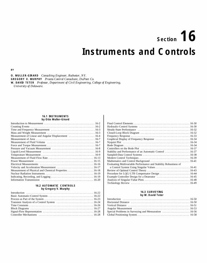
The mechanical counter is shown in Fig. 16.1.1. Motion of the eventbeing counted deflects the arm, which through an appropriate linkageadvances the count register one unit. Alternatively, motion of the actu-
Fig. 16.1.1 Mechanical counter.
MASS AND WEIGHT MEASUREMENT 16-3
ating arm may close an electrical switch which energizes a relay coil toadvance the count register one step.
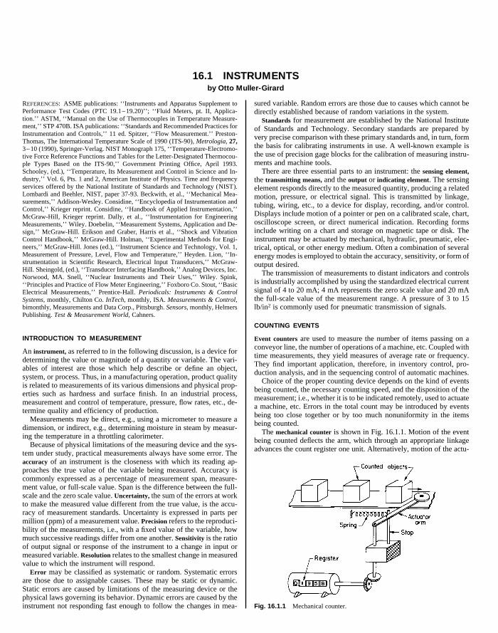
Where there is a desire to avoid contact or close proximity with theobject being counted, the photoelectric cell or diode, in conjunctionwith a lamp, a light-emitting diode (LED), or a laser light source, isemployed in the transmitted or reflected light mode (Fig. 16.1.2). Asignal to a counter is generated whenever the received light level isaltered by the passing objects. Objects may be very small and very highcounting speeds may be achieved with electronic counters.
to a fixed time. These include timers based on the charging time of acondenser (e.g., type 555 integrated circuit), and the flow of oil or otherfluid through a restriction.
Timing devices can be calibrated by comparison with a standard in-strument or by reference to the National Institute of Standards andTechnology timed radio signals, carrier frequencies and audio modula-tion of radio stations WWV and WWVB, Colorado, and WWVH,Hawaii. WWV and WWVH broadcast with carrier frequencies of 2.5, 5,10, and 15 MHz. WWV also broadcasts on 20 MHz. Broadcasts providesecond, minute, and hour marks with once-per-minute time announce-
Copyright (C) 1999 by The McGraw-Hill Companies, Inc. All rights reserved. Use ofthis product is subject to the terms of its License Agreement. Click here to view.
Fig. 16.1.2 Photoelectric counter.
Sensing methods based on electrical capacitance, magnetic, andeddy-current effects are extremely sensitive and fast acting, and aresuitable for objects in close proximity to the sensor. The capaci-tive probe senses dielectrics other than air, such as glass and plasticparts. The magnetic pickup, by induction, responds to the motion ofiron and nickel. The eddy-current sensor, by energy absorption, detectsnonmagnetic conductors. All are suitable for counting machine opera-tions.
The count is displayed by either a mechanical register as in Fig.16.1.1, a dial-type register (as on the household watthour meter), or anelectronic pulse counter with either number indicators or digital printingoutput. Electronic counters can operate accurately at rates exceeding 1million counts per second.
TIME AND FREQUENCY MEASUREMENT
Measurement of time is basic to time and motion studies, time programcontrols, and the measurements of velocity, frequency, and flow rate.(See also Sec. 1.)
Mechanical clocks, chronometers, and stopwatches measure time interms of the natural oscillation period of a system such as a pendulum,or hairspring balance-wheel combination. The minimum resolution isone-half period. Since this period is somewhat affected by temperature,precise timepieces employ a compensating element to maintain timingaccuracies over long periods. Stopwatches may be obtained to read tobetter than 0.1 s. The major limitation, however, is in the response timeof the user.
Electric timers are simple, inexpensive, and readily adaptable to re-mote-control operations. The majority of these are ac synchronousmotors geared in the proper ratio to the indicator. These depend for theiraccuracy on the frequency of the line voltage. Consequently, care mustbe exercised in using such devices for precise short-time measurements.
Electronic timers are started and stopped by electrical pulses andhence are not limited by the observer’s reaction time. They may bemade extremely accurate and capable of measuring to less than 1 ms.These measure time by counting the number of cycles in a high-fre-quency signal generated internally by means of a quartz crystal. Stop-watch versions read at 0.01 s. Commercial instruments offer one ormore functions: counting, measurement of frequency, period, and timeintervals. Microprocessor-equipped versions increase versatility.
There are a variety of timing devices designed to indicate or control
ments by voice and binary-coded decimal (BCD) signal on a 100-Hzsubcarrier. Standard audio frequencies of 440, 500, and 600 Hz areprovided. Station WWVB uses a 60-kHz carrier and provides secondand minute marks and BCD time and date. Time services are also issuedby NIST from geostationary satellites of the National Oceanographicand Atmospheric Administration (NOAA) on frequencies of 468.8375MHz for the 75° west satellite and 468.825 MHz for the 105° westsatellite. Automated Computer Time Service (ACTS) is available to300- or 1200-baud modems via phone number 303-494-4774. (See alsoSec. 1.2.)
Fast-moving, repetitive motions may be timed and studied by the useof stroboscopes which generate brilliant, very brief flashes of light at anadjustable rate.
The frequency of the observed motion is measured by adjusting thestroboscopic frequency until the system appears to stand still. The fre-quency of the motion is then equal to the stroboscope frequency or aninteger multiple of it.
Many other means exist for measuring vibrational or rotational fre-quencies. These include timing a fixed number of rotations or oscilla-tions of the moving member. Contact sensing can be done by an at-tached switch, or noncontact sensing can be done by magnetic or opticalmeans. The pulses can be counted by an electronic counter or displayedon an oscilloscope or recorder and compared with a known frequency.Also used are reeds which vibrate when the measured oscillation excitestheir natural frequencies, flyball devices which respond directly to an-gular velocity, and generator-type tachometers which generate a voltageproportional to the speed.
MASS AND WEIGHT MEASUREMENT
Mass is the measure of the quantity of matter. The fundamental unit isthe kilogram. The U.S. customary unit is the pound; 1 lb 5 0.4536 kg(see Sec. 1.2, ‘‘Measuring Units’’). Weight is a measure of the force ofgravity acting on a mass (see ‘‘Units of Force and Mass’’ in Sec. 4).
A general equation relating weight W and mass M is W/g 5 M/gc ,where g is the local acceleration of gravity, and gc 5 32.174 lbm ? ft/(lbf) (s2) [(1 kg ?m/(N) (s2)] is a property of the unit system. Then W 5Mg/gc . The specific weight w and the mass density p are related by w 5pg/gc . Masses are conveniently compared by comparing their weights,and masses are often loosely referred to as weights. Indeed, almost allpractical measures of mass are based on weight.
Weighing devices fall into two major categories: balances and force-deflection systems. The device may be batch or continuous weighing,automatic or manual. Accuracies are expected to be of the order of 0.1to better than 0.0001 percent, depending on the type and application ofthe scale. Calibration is normally performed by use of standard weights(masses) with calibrations traceable to the National Institute of Stan-dards and Technology.
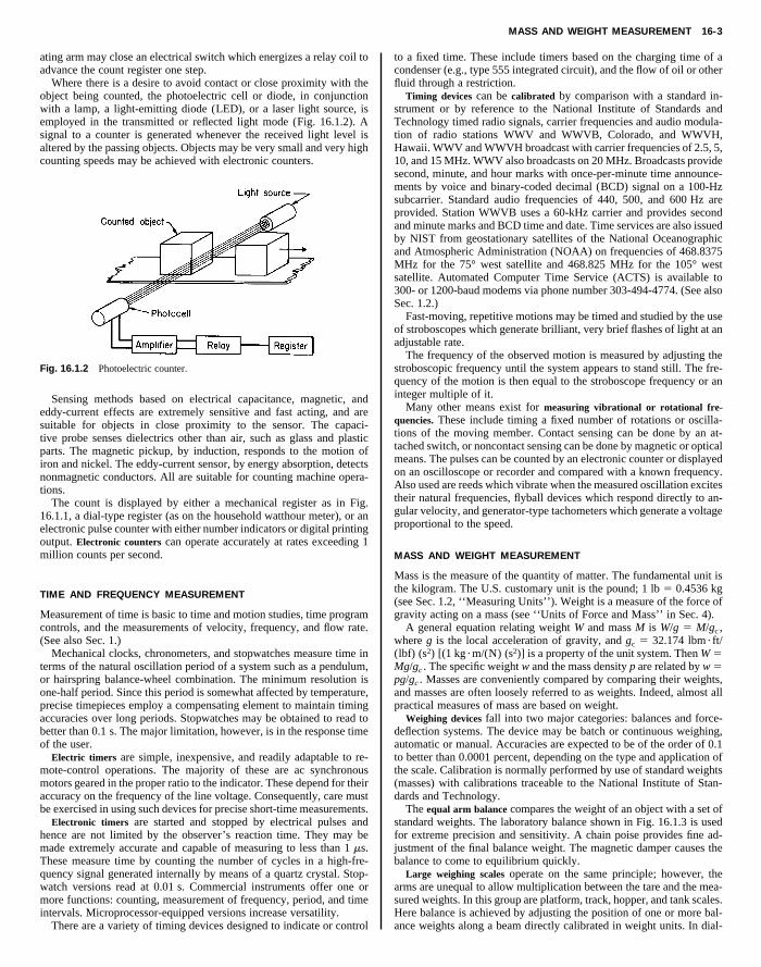
The equal arm balance compares the weight of an object with a set ofstandard weights. The laboratory balance shown in Fig. 16.1.3 is usedfor extreme precision and sensitivity. A chain poise provides fine ad-justment of the final balance weight. The magnetic damper causes thebalance to come to equilibrium quickly.
Large weighing scales operate on the same principle; however, thearms are unequal to allow multiplication between the tare and the mea-sured weights. In this group are platform, track, hopper, and tank scales.Here balance is achieved by adjusting the position of one or more bal-ance weights along a beam directly calibrated in weight units. In dial-
16-4 INSTRUMENTS
indicating-type scales, balance is achieved automatically through thedeflection of calibrated pendulum weights from the vertical. The de-flection is greatly magnified by the pointer-actuating mechanism, pro-viding a direct-reading weight indication on the dial.
In continuous weighers, a section of conveyor belt is balanced on aweigh beam (Fig. 16.1.5). The belt is driven at a constant speed; hence,if the total weight is held constant, the weight rate of material fedthrough the scale is fixed. Unbalance of the weight beam causes the rateof material flow onto the belt to be changed in the direction of restoringbalance. This is accomplished by a mechanical adjustment of the feedgate or by varying the speed of a belt or screw feeder drive.
Copyright (C) 1999 by The McGraw-Hill Companies, Inc. All rights reserved. Use ofthis product is subject to the terms of its License Agreement. Click here to view.
Fig. 16.1.3 Laboratory balance.
Since the deflection of a spring (within its design range) is directlyproportional to the applied force, a calibrated spring serves as a simpleand inexpensive weighing device. Applications include the spring scaleand torsion balance. These are subject to hysteresis and temperatureerrors and are not used for precise work.
Other force-sensing elements are adaptable to weight measurement.Strain-gage load cells eliminate pivot maintenance and moving partsand provide an electrical output which can be used for direct recordingand control purposes. Pneumatic pressure cells are also used with simi-lar advantages.
In production processes, continuous and automatic operating scales areemployed. In one type, the balancing weight is positioned by a revers-ible electric motor. Deflection of the beam makes an electrical contactwhich drives the motor in the proper direction to restore balance. Thefinal balance position is translated by means of a potentiometer or digi-tal encoding disk into a signal which is used for recording or controlpurposes.
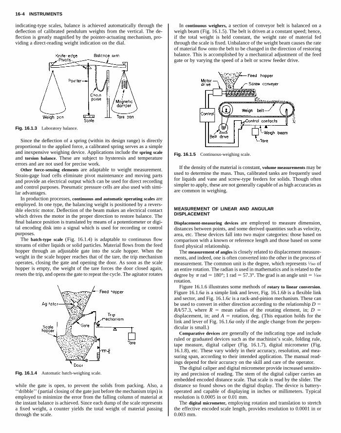
The batch-type scale (Fig. 16.1.4) is adaptable to continuous flowstreams of either liquids or solid particles. Material flows from the feedhopper through an adjustable gate into the scale hopper. When theweight in the scale hopper reaches that of the tare, the trip mechanismoperates, closing the gate and opening the door. As soon as the scalehopper is empty, the weight of the tare forces the door closed again,resets the trip, and opens the gate to repeat the cycle. The agitator rotates
Fig. 16.1.4 Automatic batch-weighing scale.
while the gate is open, to prevent the solids from packing. Also, a‘‘dribble’’ (partial closing of the gate just before the mechanism trips) isemployed to minimize the error from the falling column of material atthe instant balance is achieved. Since each dump of the scale representsa fixed weight, a counter yields the total weight of material passingthrough the scale.
Fig. 16.1.5 Continuous-weighing scale.
If the density of the material is constant, volume measurements may beused to determine the mass. Thus, calibrated tanks are frequently usedfor liquids and vane and screw-type feeders for solids. Though oftensimpler to apply, these are not generally capable of as high accuracies asare common in weighing.
MEASUREMENT OF LINEAR AND ANGULARDISPLACEMENT
Displacement-measuring devices are employed to measure dimension,distances between points, and some derived quantities such as velocity,area, etc. These devices fall into two major categories: those based oncomparison with a known or reference length and those based on somefixed physical relationship.
The measurement of angles is closely related to displacement measure-ments, and indeed, one is often converted into the other in the process ofmeasurement. The common unit is the degree, which represents 1⁄360 ofan entire rotation. The radian is used in mathematics and is related to thedegree by p rad 5 180°; 1 rad 5 57.3°. The grad is an angle unit 5 1⁄400
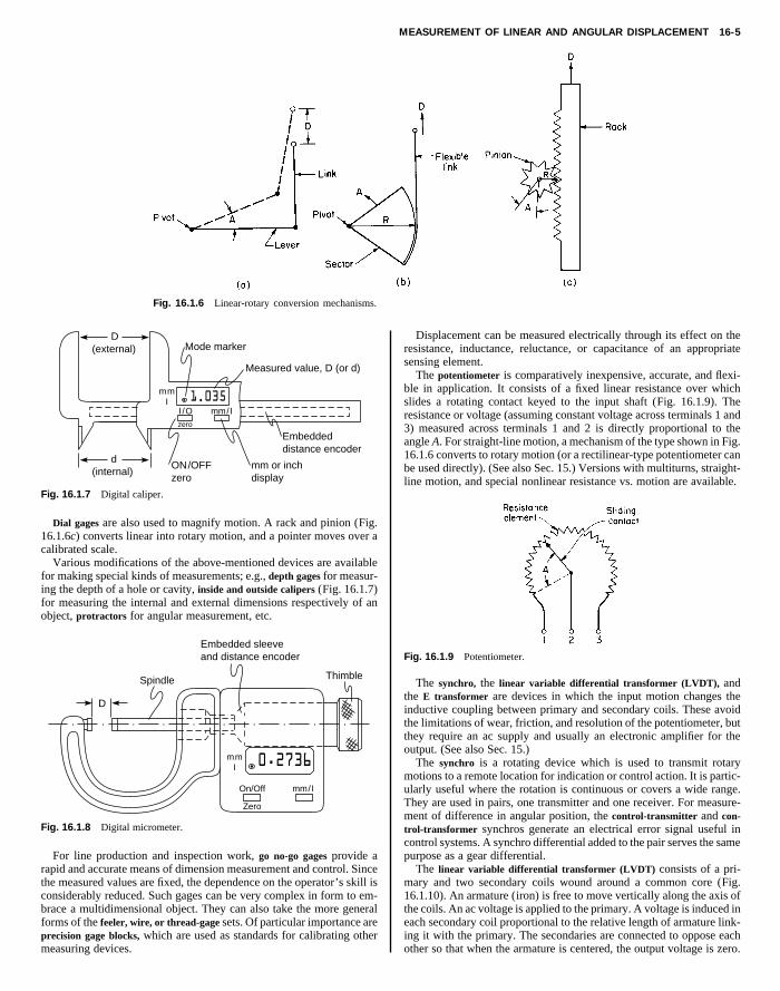
rotation.Figure 16.1.6 illustrates some methods of rotary to linear conversion.
Figure 16.1.6a is a simple link and lever, Fig. 16.1.6b is a flexible linkand sector, and Fig. 16.1.6c is a rack-and-pinion mechanism. These canbe used to convert in either direction according to the relationship D 5RA/57.3, where R 5 mean radius of the rotating element, in; D 5displacement, in; and A 5 rotation, deg. (This equation holds for thelink and lever of Fig. 16.1.6a only if the angle change from the perpen-dicular is small.)
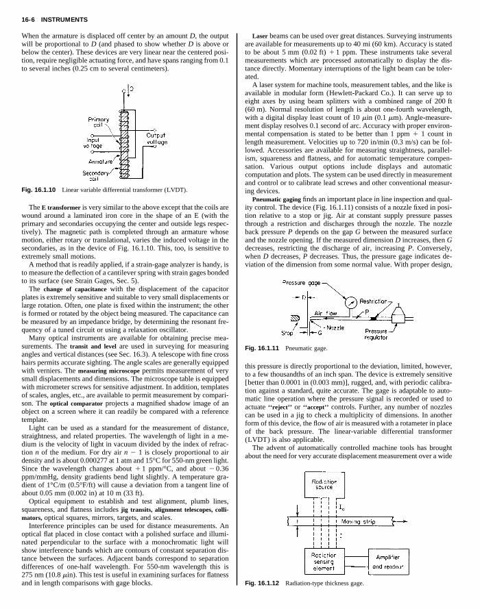
Comparative devices are generally of the indicating type and includeruled or graduated devices such as the machinist’s scale, folding rule,tape measure, digital caliper (Fig. 16.1.7), digital micrometer (Fig.16.1.8), etc. These vary widely in their accuracy, resolution, and mea-suring span, according to their intended application. The manual read-ings depend for their accuracy on the skill and care of the operator.
The digital caliper and digital micrometer provide increased sensitiv-ity and precision of reading. The stem of the digital caliper carries anembedded encoded distance scale. That scale is read by the slider. Thedistance so found shows on the digital display. The device is battery-operated and capable of displaying in inches or millimeters. Typicalresolution is 0.0005 in or 0.01 mm.
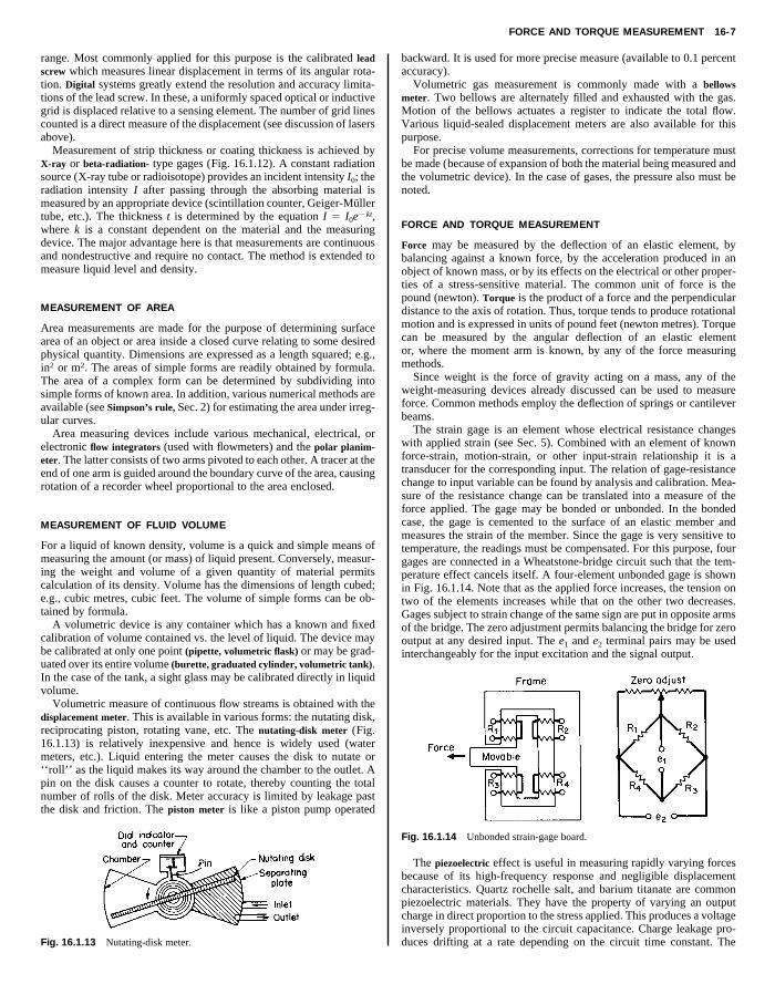
The digital micrometer, employing rotation and translation to stretchthe effective encoded scale length, provides resolution to 0.0001 in or0.003 mm.
MEASUREMENT OF LINEAR AND ANGULAR DISPLACEMENT 16-5
Fig. 16.1.6 Linear-rotary conversion mechanisms.
Mode marker
mmI
I/Ozero
mm/I
Embeddeddistance encoder
Measured value, D (or d)
D(external)
d
1.035
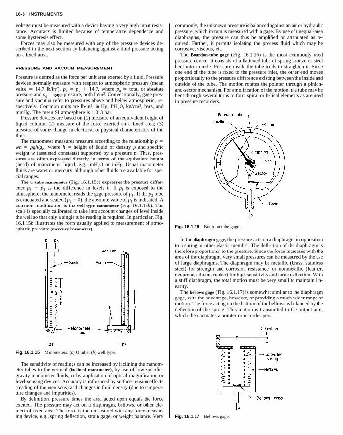
Displacement can be measured electrically through its effect on theresistance, inductance, reluctance, or capacitance of an appropriatesensing element.
The potentiometer is comparatively inexpensive, accurate, and flexi-ble in application. It consists of a fixed linear resistance over whichslides a rotating contact keyed to the input shaft (Fig. 16.1.9). Theresistance or voltage (assuming constant voltage across terminals 1 and3) measured across terminals 1 and 2 is directly proportional to theangle A. For straight-line motion, a mechanism of the type shown in Fig.16.1.6 converts to rotary motion (or a rectilinear-type potentiometer can
Copyright (C) 1999 by The McGraw-Hill Companies, Inc. All rights reserved. Use ofthis product is subject to the terms of its License Agreement. Click here to view.
mm or inchdisplay
ON/OFFzero
(internal)
Fig. 16.1.7 Digital caliper.
Dial gages are also used to magnify motion. A rack and pinion (Fig.16.1.6c) converts linear into rotary motion, and a pointer moves over acalibrated scale.
Various modifications of the above-mentioned devices are availablefor making special kinds of measurements; e.g., depth gages for measur-ing the depth of a hole or cavity, inside and outside calipers (Fig. 16.1.7)for measuring the internal and external dimensions respectively of anobject, protractors for angular measurement, etc.
mmI
mm/IOn/Off
Zero
D
Spindle
Embedded sleeveand distance encoder
Thimble
0.2736
. . . . . . . . . .
Fig. 16.1.8 Digital micrometer.
For line production and inspection work, go no-go gages provide arapid and accurate means of dimension measurement and control. Sincethe measured values are fixed, the dependence on the operator’s skill isconsiderably reduced. Such gages can be very complex in form to em-brace a multidimensional object. They can also take the more generalforms of the feeler, wire, or thread-gage sets. Of particular importance areprecision gage blocks, which are used as standards for calibrating othermeasuring devices.
be used directly). (See also Sec. 15.) Versions with multiturns, straight-line motion, and special nonlinear resistance vs. motion are available.
Fig. 16.1.9 Potentiometer.
The synchro, the linear variable differential transformer (LVDT), andthe E transformer are devices in which the input motion changes theinductive coupling between primary and secondary coils. These avoidthe limitations of wear, friction, and resolution of the potentiometer, butthey require an ac supply and usually an electronic amplifier for theoutput. (See also Sec. 15.)
The synchro is a rotating device which is used to transmit rotarymotions to a remote location for indication or control action. It is partic-ularly useful where the rotation is continuous or covers a wide range.They are used in pairs, one transmitter and one receiver. For measure-ment of difference in angular position, the control-transmitter and con-trol-transformer synchros generate an electrical error signal useful incontrol systems. A synchro differential added to the pair serves the samepurpose as a gear differential.
The linear variable differential transformer (LVDT) consists of a pri-mary and two secondary coils wound around a common core (Fig.16.1.10). An armature (iron) is free to move vertically along the axis ofthe coils. An ac voltage is applied to the primary. A voltage is induced ineach secondary coil proportional to the relative length of armature link-ing it with the primary. The secondaries are connected to oppose eachother so that when the armature is centered, the output voltage is zero.
16-6 INSTRUMENTS
When the armature is displaced off center by an amount D, the outputwill be proportional to D (and phased to show whether D is above orbelow the center). These devices are very linear near the centered posi-tion, require negligible actuating force, and have spans ranging from 0.1to several inches (0.25 cm to several centimeters).
Laser beams can be used over great distances. Surveying instrumentsare available for measurements up to 40 mi (60 km). Accuracy is statedto be about 5 mm (0.02 ft) 1 1 ppm. These instruments take severalmeasurements which are processed automatically to display the dis-tance directly. Momentary interruptions of the light beam can be toler-ated.
A laser system for machine tools, measurement tables, and the like isavailable in modular form (Hewlett-Packard Co.). It can serve up toeight axes by using beam splitters with a combined range of 200 ft(60 m). Normal resolution of length is about one-fourth wavelength,
Copyright (C) 1999 by The McGraw-Hill Companies, Inc. All rights reserved. Use ofthis product is subject to the terms of its License Agreement. Click here to view.
Fig. 16.1.10 Linear variable differential transformer (LVDT).
The E transformer is very similar to the above except that the coils arewound around a laminated iron core in the shape of an E (with theprimary and secondaries occupying the center and outside legs respec-tively). The magnetic path is completed through an armature whosemotion, either rotary or translational, varies the induced voltage in thesecondaries, as in the device of Fig. 16.1.10. This, too, is sensitive toextremely small motions.
A method that is readily applied, if a strain-gage analyzer is handy, isto measure the deflection of a cantilever spring with strain gages bondedto its surface (see Strain Gages, Sec. 5).
The change of capacitance with the displacement of the capacitorplates is extremely sensitive and suitable to very small displacements orlarge rotation. Often, one plate is fixed within the instrument; the otheris formed or rotated by the object being measured. The capacitance canbe measured by an impedance bridge, by determining the resonant fre-quency of a tuned circuit or using a relaxation oscillator.
Many optical instruments are available for obtaining precise mea-surements. The transit and level are used in surveying for measuringangles and vertical distances (see Sec. 16.3). A telescope with fine crosshairs permits accurate sighting. The angle scales are generally equippedwith verniers. The measuring microscope permits measurement of verysmall displacements and dimensions. The microscope table is equippedwith micrometer screws for sensitive adjustment. In addition, templatesof scales, angles, etc., are available to permit measurement by compari-son. The optical comparator projects a magnified shadow image of anobject on a screen where it can readily be compared with a referencetemplate.
Light can be used as a standard for the measurement of distance,straightness, and related properties. The wavelength of light in a me-dium is the velocity of light in vacuum divided by the index of refrac-tion n of the medium. For dry air n 2 1 is closely proportional to airdensity and is about 0.000277 at 1 atm and 15°C for 550-nm green light.Since the wavelength changes about 1 1 ppm/°C, and about 2 0.36ppm/mmHg, density gradients bend light slightly. A temperature gra-dient of 1°C/m (0.5°F/ft) will cause a deviation from a tangent line ofabout 0.05 mm (0.002 in) at 10 m (33 ft).
Optical equipment to establish and test alignment, plumb lines,squareness, and flatness includes jig transits, alignment telescopes, colli-mators, optical squares, mirrors, targets, and scales.
Interference principles can be used for distance measurements. Anoptical flat placed in close contact with a polished surface and illumi-nated perpendicular to the surface with a monochromatic light willshow interference bands which are contours of constant separation dis-tance between the surfaces. Adjacent bands correspond to separationdifferences of one-half wavelength. For 550-nm wavelength this is275 nm (10.8 min). This test is useful in examining surfaces for flatnessand in length comparisons with gage blocks.
with a digital display least count of 10 min (0.1 mm). Angle-measure-ment display resolves 0.1 second of arc. Accuracy with proper environ-mental compensation is stated to be better than 1 ppm 1 1 count inlength measurement. Velocities up to 720 in/min (0.3 m/s) can be fol-lowed. Accessories are available for measuring straightness, parallel-ism, squareness and flatness, and for automatic temperature compen-sation. Various output options include displays and automaticcomputation and plots. The system can be used directly in measurementand control or to calibrate lead screws and other conventional measur-ing devices.
Pneumatic gaging finds an important place in line inspection and qual-ity control. The device (Fig. 16.1.11) consists of a nozzle fixed in posi-tion relative to a stop or jig. Air at constant supply pressure passesthrough a restriction and discharges through the nozzle. The nozzleback pressure P depends on the gap G between the measured surfaceand the nozzle opening. If the measured dimension D increases, then Gdecreases, restricting the discharge of air, increasing P. Conversely,when D decreases, P decreases. Thus, the pressure gage indicates de-viation of the dimension from some normal value. With proper design,
Fig. 16.1.11 Pneumatic gage.
this pressure is directly proportional to the deviation, limited, however,to a few thousandths of an inch span. The device is extremely sensitive[better than 0.0001 in (0.003 mm)], rugged, and, with periodic calibra-tion against a standard, quite accurate. The gage is adaptable to auto-matic line operation where the pressure signal is recorded or used toactuate ‘‘reject’’ or ‘‘accept’’ controls. Further, any number of nozzlescan be used in a jig to check a multiplicity of dimensions. In anotherform of this device, the flow of air is measured with a rotameter in placeof the back pressure. The linear-variable differential transformer(LVDT) is also applicable.
The advent of automatically controlled machine tools has broughtabout the need for very accurate displacement measurement over a wide
Fig. 16.1.12 Radiation-type thickness gage.
FORCE AND TORQUE MEASUREMENT 16-7
range. Most commonly applied for this purpose is the calibrated leadscrew which measures linear displacement in terms of its angular rota-tion. Digital systems greatly extend the resolution and accuracy limita-tions of the lead screw. In these, a uniformly spaced optical or inductivegrid is displaced relative to a sensing element. The number of grid linescounted is a direct measure of the displacement (see discussion of lasersabove).
Measurement of strip thickness or coating thickness is achieved byX-ray or beta-radiation- type gages (Fig. 16.1.12). A constant radiationsource (X-ray tube or radioisotope) provides an incident intensity I0; the
backward. It is used for more precise measure (available to 0.1 percentaccuracy).
Volumetric gas measurement is commonly made with a bellowsmeter. Two bellows are alternately filled and exhausted with the gas.Motion of the bellows actuates a register to indicate the total flow.Various liquid-sealed displacement meters are also available for thispurpose.
For precise volume measurements, corrections for temperature mustbe made (because of expansion of both the material being measured andthe volumetric device). In the case of gases, the pressure also must be
Copyright (C) 1999 by The McGraw-Hill Companies, Inc. All rights reserved. Use ofthis product is subject to the terms of its License Agreement. Click here to view.
radiation intensity I after passing through the absorbing material ismeasured by an appropriate device (scintillation counter, Geiger-Mullertube, etc.). The thickness t is determined by the equation I 5 I0e2 kt,where k is a constant dependent on the material and the measuringdevice. The major advantage here is that measurements are continuousand nondestructive and require no contact. The method is extended tomeasure liquid level and density.
MEASUREMENT OF AREA
Area measurements are made for the purpose of determining surfacearea of an object or area inside a closed curve relating to some desiredphysical quantity. Dimensions are expressed as a length squared; e.g.,in2 or m2. The areas of simple forms are readily obtained by formula.The area of a complex form can be determined by subdividing intosimple forms of known area. In addition, various numerical methods areavailable (see Simpson’s rule, Sec. 2) for estimating the area under irreg-ular curves.
Area measuring devices include various mechanical, electrical, orelectronic flow integrators (used with flowmeters) and the polar planim-eter. The latter consists of two arms pivoted to each other. A tracer at theend of one arm is guided around the boundary curve of the area, causingrotation of a recorder wheel proportional to the area enclosed.
MEASUREMENT OF FLUID VOLUME
For a liquid of known density, volume is a quick and simple means ofmeasuring the amount (or mass) of liquid present. Conversely, measur-ing the weight and volume of a given quantity of material permitscalculation of its density. Volume has the dimensions of length cubed;e.g., cubic metres, cubic feet. The volume of simple forms can be ob-tained by formula.
A volumetric device is any container which has a known and fixedcalibration of volume contained vs. the level of liquid. The device maybe calibrated at only one point (pipette, volumetric flask) or may be grad-uated over its entire volume (burette, graduated cylinder, volumetric tank).In the case of the tank, a sight glass may be calibrated directly in liquidvolume.
Volumetric measure of continuous flow streams is obtained with thedisplacement meter. This is available in various forms: the nutating disk,reciprocating piston, rotating vane, etc. The nutating-disk meter (Fig.16.1.13) is relatively inexpensive and hence is widely used (watermeters, etc.). Liquid entering the meter causes the disk to nutate or‘‘roll’’ as the liquid makes its way around the chamber to the outlet. Apin on the disk causes a counter to rotate, thereby counting the totalnumber of rolls of the disk. Meter accuracy is limited by leakage pastthe disk and friction. The piston meter is like a piston pump operated
Fig. 16.1.13 Nutating-disk meter.
noted.
FORCE AND TORQUE MEASUREMENT
Force may be measured by the deflection of an elastic element, bybalancing against a known force, by the acceleration produced in anobject of known mass, or by its effects on the electrical or other proper-ties of a stress-sensitive material. The common unit of force is thepound (newton). Torque is the product of a force and the perpendiculardistance to the axis of rotation. Thus, torque tends to produce rotationalmotion and is expressed in units of pound feet (newton metres). Torquecan be measured by the angular deflection of an elastic elementor, where the moment arm is known, by any of the force measuringmethods.
Since weight is the force of gravity acting on a mass, any of theweight-measuring devices already discussed can be used to measureforce. Common methods employ the deflection of springs or cantileverbeams.
The strain gage is an element whose electrical resistance changeswith applied strain (see Sec. 5). Combined with an element of knownforce-strain, motion-strain, or other input-strain relationship it is atransducer for the corresponding input. The relation of gage-resistancechange to input variable can be found by analysis and calibration. Mea-sure of the resistance change can be translated into a measure of theforce applied. The gage may be bonded or unbonded. In the bondedcase, the gage is cemented to the surface of an elastic member andmeasures the strain of the member. Since the gage is very sensitive totemperature, the readings must be compensated. For this purpose, fourgages are connected in a Wheatstone-bridge circuit such that the tem-perature effect cancels itself. A four-element unbonded gage is shownin Fig. 16.1.14. Note that as the applied force increases, the tension ontwo of the elements increases while that on the other two decreases.Gages subject to strain change of the same sign are put in opposite armsof the bridge. The zero adjustment permits balancing the bridge for zerooutput at any desired input. The e1 and e2 terminal pairs may be usedinterchangeably for the input excitation and the signal output.
Fig. 16.1.14 Unbonded strain-gage board.
The piezoelectric effect is useful in measuring rapidly varying forcesbecause of its high-frequency response and negligible displacementcharacteristics. Quartz rochelle salt, and barium titanate are commonpiezoelectric materials. They have the property of varying an outputcharge in direct proportion to the stress applied. This produces a voltageinversely proportional to the circuit capacitance. Charge leakage pro-duces drifting at a rate depending on the circuit time constant. The
16-8 INSTRUMENTS
voltage must be measured with a device having a very high input resis-tance. Accuracy is limited because of temperature dependence andsome hysteresis effect.
Forces may also be measured with any of the pressure devices de-scribed in the next section by balancing against a fluid pressure actingon a fixed area.
PRESSURE AND VACUUM MEASUREMENT
Pressure is defined as the force per unit area exerted by a fluid. Pressure
commonly, the unknown pressure is balanced against an air or hydraulicpressure, which in turn is measured with a gage. By use of unequal-areadiaphragms, the pressure can thus be amplified or attenuated as re-quired. Further, it permits isolating the process fluid which may becorrosive, viscous, etc.
The Bourdon-tube gage (Fig. 16.1.16) is the most commonly usedpressure device. It consists of a flattened tube of spring bronze or steelbent into a circle. Pressure inside the tube tends to straighten it. Sinceone end of the tube is fixed to the pressure inlet, the other end movesproportionally to the pressure difference existing between the inside and
Copyright (C) 1999 by The McGraw-Hill Companies, Inc. All rights reserved. Use ofthis product is subject to the terms of its License Agreement. Click here to view.
devices normally measure with respect to atmospheric pressure (meanvalue 5 14.7 lb/in2), pa 5 pg 1 14.7, where pa 5 total or absolutepressure and pg 5 gage pressure, both lb/in2. Conventionally, gage pres-sure and vacuum refer to pressures above and below atmospheric, re-spectively. Common units are lb/in2, in Hg, ftH2O, kg/cm2, bars, andmmHg. The mean SI atmosphere is 1.013 bar.
Pressure devices are based on (1) measure of an equivalent height ofliquid column; (2) measure of the force exerted on a fixed area; (3)measure of some change in electrical or physical characteristics of thefluid.
The manometer measures pressure according to the relationship p 5wh 5 rgh/gc , where h 5 height of liquid of density r and specificweight w (assumed constants) supported by a pressure p. Thus, pres-sures are often expressed directly in terms of the equivalent height(head) of manometer liquid, e.g., inH2O or inHg. Usual manometerfluids are water or mercury, although other fluids are available for spe-cial ranges.
The U-tube manometer (Fig. 16.1.15a) expresses the pressure differ-ence p1 2 p2 as the difference in levels h. If p2 is exposed to theatmosphere, the manometer reads the gage pressure of p1 . If the p2 tubeis evacuated and sealed (p2 5 0), the absolute value of p1 is indicated. Acommon modification is the well-type manometer (Fig. 16.1.15b). Thescale is specially calibrated to take into account changes of level insidethe well so that only a single tube reading is required. In particular, Fig.16.1.15b illustrates the form usually applied to measurement of atmo-spheric pressure (mercury barometer).
Fig. 16.1.15 Manometers. (a) U tube; (b) well type.
The sensitivity of readings can be increased by inclining the manom-eter tubes to the vertical (inclined manometer), by use of low-specific-gravity manometer fluids, or by application of optical-magnification orlevel-sensing devices. Accuracy is influenced by surface-tension effects(reading of the meniscus) and changes in fluid density (due to tempera-ture changes and impurities).
By definition, pressure times the area acted upon equals the forceexerted. The pressure may act on a diaphragm, bellows, or other ele-ment of fixed area. The force is then measured with any force-measur-ing device, e.g., spring deflection, strain gage, or weight balance. Very
outside of the tube. The motion rotates the pointer through a pinion-and-sector mechanism. For amplification of the motion, the tube may bebent through several turns to form spiral or helical elements as are usedin pressure recorders.
Fig. 16.1.16 Bourdon-tube gage.
In the diaphragm gage, the pressure acts on a diaphragm in oppositionto a spring or other elastic member. The deflection of the diaphragm istherefore proportional to the pressure. Since the force increases with thearea of the diaphragm, very small pressures can be measured by the useof large diaphragms. The diaphragm may be metallic (brass, stainlesssteel) for strength and corrosion resistance, or nonmetallic (leather,neoprene, silicon, rubber) for high sensitivity and large deflection. Witha stiff diaphragm, the total motion must be very small to maintain lin-earity.
The bellows gage (Fig. 16.1.17) is somewhat similar to the diaphragmgage, with the advantage, however, of providing a much wider range ofmotion. The force acting on the bottom of the bellows is balanced by thedeflection of the spring. This motion is transmitted to the output arm,which then actuates a pointer or recorder pen.
Fig. 16.1.17 Bellows gage.
TEMPERATURE MEASUREMENT 16-9
The motion (or force) of the pressure element can be converted intoan electrical signal by use of a differential transformer or strain-gageelement or into an air-pressure signal through the action of a nozzle andpilot. The signal is then used for transmission, recording, or control.
The dead-weight tester is used as a standard for calibrating gages.Known hydraulic or gas pressures are generated by means of weightsloaded on a calibrated piston. The useful range is from 5 to 5,000 lb/in2
(0.3 to 350 bar). For low pressures, the water or mercury manometerserves as a reference.
For many applications (fluid flow, liquid level), it is important to
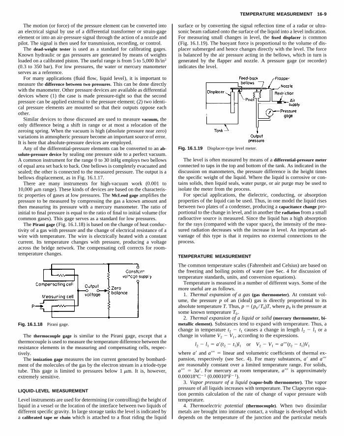
surface or by converting the signal reflection time of a radar or ultra-sonic beam radiated onto the surface of the liquid into a level indication.For measuring small changes in level, the fixed displacer is common(Fig. 16.1.19). The buoyant force is proportional to the volume of dis-placer submerged and hence changes directly with the level. The forceis balanced by the air pressure acting in the bellows, which in turn isgenerated by the flapper and nozzle. A pressure gage (or recorder)indicates the level.
Copyright (C) 1999 by The McGraw-Hill Companies, Inc. All rights reserved. Use ofthis product is subject to the terms of its License Agreement. Click here to view.
measure the difference between two pressures. This can be done directlywith the manometer. Other pressure devices are available as differentialdevices where (1) the case is made pressure-tight so that the secondpressure can be applied external to the pressure element; (2) two identi-cal pressure elements are mounted so that their outputs oppose eachother.
Similar devices to those discussed are used to measure vacuum, theonly difference being a shift in range or at most a relocation of thezeroing spring. When the vacuum is high (absolute pressure near zero)variations in atmospheric pressure become an important source of error.It is here that absolute-pressure devices are employed.
Any of the differential-pressure elements can be converted to an ab-solute-pressure device by sealing one pressure side to a perfect vacuum.A common instrument for the range 0 to 30 inHg employs two bellowsof equal area set back to back. One bellows is completely evacuated andsealed; the other is connected to the measured pressure. The output is abellows displacement, as in Fig. 16.1.17.
There are many instruments for high-vacuum work (0.001 to10,000 mm range). These kinds of devices are based on the characteris-tic properties of gases at low pressures. The McLeod gage amplifies thepressure to be measured by compressing the gas a known amount andthen measuring its pressure with a mercury manometer. The ratio ofinitial to final pressure is equal to the ratio of final to initial volume (forcommon gases). This gage serves as a standard for low pressures.
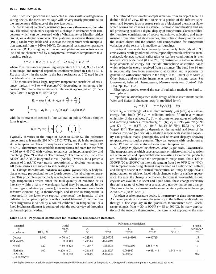
The Pirani gage (Fig. 16.1.18) is based on the change of heat conduc-tivity of a gas with pressure and the change of electrical resistance of awire with temperature. The wire is electrically heated with a constantcurrent. Its temperature changes with pressure, producing a voltageacross the bridge network. The compensating cell corrects for room-temperature changes.
Fig. 16.1.18 Pirani gage.
The thermocouple gage is similar to the Pirani gage, except that athermocouple is used to measure the temperature difference between theresistance elements in the measuring and compensating cells, respec-tively.
The ionization gage measures the ion current generated by bombard-ment of the molecules of the gas by the electron stream in a triode-typetube. This gage is limited to pressures below 1 mm. It is, however,extremely sensitive.
LIQUID-LEVEL MEASUREMENT
Level instruments are used for determining (or controlling) the height ofliquid in a vessel or the location of the interface between two liquids ofdifferent specific gravity. In large storage tanks the level is indicated bya calibrated tape or chain which is attached to a float riding the liquid
Fig. 16.1.19 Displacer-type level meter.
The level is often measured by means of a differential-pressure meterconnected to taps in the top and bottom of the tank. As indicated in thediscussion on manometers, the pressure difference is the height timesthe specific weight of the liquid. Where the liquid is corrosive or con-tains solids, then liquid seals, water purge, or air purge may be used toisolate the meter from the process.
For special applications, the dielectric, conducting, or absorptionproperties of the liquid can be used. Thus, in one model the liquid risesbetween two plates of a condenser, producing a capacitance change pro-portional to the change in level, and in another the radiation from a smallradioactive source is measured. Since the liquid has a high absorptionfor the rays (compared with the vapor space), the intensity of the mea-sured radiation decreases with the increase in level. An important ad-vantage of this type is that it requires no external connections to theprocess.
TEMPERATURE MEASUREMENT
The common temperature scales (Fahrenheit and Celsius) are based onthe freezing and boiling points of water (see Sec. 4 for discussion oftemperature standards, units, and conversion equations).
Temperature is measured in a number of different ways. Some of themore useful are as follows.
1. Thermal expansion of a gas (gas thermometer). At constant vol-ume, the pressure p of an (ideal) gas is directly proportional to itsabsolute temperature T. Thus, p 5 (p0 /T0)T, where p0 is the pressure atsome known temperature T0 .
2. Thermal expansion of a liquid or solid (mercury thermometer, bi-metallic element). Substances tend to expand with temperature. Thus, achange in temperature t2 2 t1 causes a change in length l2 2 l1 or achange in volume V2 2 V1 , according to the expressions.
l2 2 l1 5 a9(t2 2 t1)l1 or V2 2 V1 5 a999(t2 2 t1)V1
where a9 and a999 5 linear and volumetric coefficients of thermal ex-pansion, respectively (see Sec. 4). For many substances, a9 and a999are reasonably constant over a limited temperature range. For solids,a999 5 3a9. For mercury at room temperature, a999 is approximately0.00018°C2 1 (0.00010°F2 1).
3. Vapor pressure of a liquid (vapor-bulb thermometer). The vaporpressure of all liquids increases with temperature. The Clapeyron equa-tion permits calculation of the rate of change of vapor pressure withtemperature.
4. Thermoelectric potential (thermocouple). When two dissimilarmetals are brought into intimate contact, a voltage is developed whichdepends on the temperature of the junction and the particular metals
16-10 INSTRUMENTS
used. If two such junctions are connected in series with a voltage-mea-suring device, the measured voltage will be very nearly proportional tothe temperature difference of the two junctions.
5. Variation of electrical resistance (resistance thermometer, thermis-tor). Electrical conductors experience a change in resistance with tem-perature which can be measured with a Wheatstone- or Mueller-bridgecircuit, or a digital ohmmeter. The platinum resistance thermometer(PRT) can be very stable and is used as the temperature scale interpola-tion standard from 2 160 to 660°C. Commercial resistance temperaturedetectors (RTD) using copper, nickel, and platinum conductors are in
The infrared thermometer accepts radiation from an object seen in adefinite field of view, filters it to select a portion of the infrared spec-trum, and focuses it on a sensor such as a blackened thermistor flake,which warms and changes resistance. Electronic amplification and sig-nal processing produce a digital display of temperature. Correct calibra-tion requires consideration of source emissivity, reflection, and trans-mission from other radiation sources, atmospheric absorption betweenthe source object and the sensor, and compensation for temperaturevariation at the sensor’s immediate surroundings.
Electrical nonconductors generally have fairly high (about 0.95)
ec
BC/
.30
.95
55
13
Copyright (C) 1999 by The McGraw-Hill Companies, Inc. All rights reserved. Use ofthis product is subject to the terms of its License Agreement. Click here to view.
use and are characterized by a polynomial resistance-temperature rela-tionship, such as
t 5 A 1 B 3 Rt 1 C 3 Rt2 1 D 3 Rt
3 1 E 3 Rt4
where Rt 5 resistance at prevailing temperature t in °C. A, B, C, D, andE are range- and material-dependent coefficients listed in Table 16.1.1.R0 , also shown in the table, is the base resistance at 0°C used in theidentification of the sensor.
The thermistor has a large, negative temperature coefficient of resis-tance, typically 2 3 to 2 6 percent /°C, decreasing as temperature in-creases. The temperature-resistance relation is approximated (to per-haps 0.01° in range 0 to 100°C) by:
Rt 5 expSA0 1 A1 /t 1A2
t21
A3
t3Dand
l
t5 a0 1 a1 ln Rt 1 a2(ln Rt)2 1 a3(ln Rt)3
with the constants chosen to fit four calibration points. Often a simplerform is given:
R 5 R0 expHbFSl
tD 2S l
t0DGJ
.Typically b varies in the range of 3,000 to 5,000 K. The referencetemperature t0 is usually 298 K(5 25°C, 77°F), and R0 is the resistanceat that temperature. The error may be as small as 0.3°C in the range of 0°to 50°C. Thermistors are available in many forms and sizes for use from2 196 to 1 450°C with various tolerances on interchangeability andmatching. (See ‘‘Catalog of Thermistors,’’ Thermometrics, Inc.) TheAD590 and AD592 integrated circuit (Analog Devices, Inc.) passes acurrent of 1 mA/°K very nearly proportional to absolute temperature.All these sensors are subject to self-heating error.
6. Change in radiation (radiation and optical pyrometers). A body ra-diates energy proportional to the fourth power of its absolute tempera-ture. This principle is particularly adaptable to the measurement of veryhigh temperatures where either the total quantity of radiation or itsintensity within a narrow wavelength band may be measured. In theformer type (radiation pyrometer), the radiation is focused on a heat-sensitive element, e.g., a thermocouple, and its rise in temperature ismeasured. In the latter type (optical pyrometer) the intensity of theradiation is compared optically with a heated filament. Either the fila-ment brightness is varied by a control calibrated in temperature, or afixed brightness filament is compared with the source viewed through acalibrated optical wedge.
Table 16.1.1 Polynomial Coefficients for Resistance Temperature Det
A,°C °
Materialof
conductor ID R0 , V
Usefulrange,°C
Copper 9.042 2 70 to 0 2 225.64 2310V @25°C 0 to 150 2 234.69 25
Nickel 120 2 80 to 320 2 199.47 1.9
Platinum 100 2 200 to 0 2 241.86 2.2
DIN/IEC 0 to 850 2 236.06 2.215a 5 0.00385/°C
* For higher accuracy consult the table or equation furnished by the manufacturer of the specific
emissivities, while good conductors (especially smooth, reflective metalsurfaces), do not; special calibration or surface conditioning is thenneeded. Very wide band (0.7 to 20 mm) instruments gather relativelylarge amounts of energy but include atmospheric absorption bandswhich reduce the energy received from a distance. The band 8 to 14 mmis substantially free from atmospheric absorption and is popular forgeneral use with source objects in the range 32 to 1,000°F (0 to 540°C).Other bands and two-color instruments are used in some cases. SeeBonkowski, Infrared Thermometry, Measurements and Control, Feb.1984, pp. 152–162.
Fiber-optics probes extend the use of radiation methods to hard-to-reach places.
Important relationships used in the design of these instruments are theWien and Stefan-Boltzmann laws (in modified form):
lm 5 k1/T q 5 k2«A(T42 2 T4
1)
where lm 5 wavelength of maximum intensity, mm (nm); q 5 radiantenergy flux, Btu/h (W); A 5 radiation surface, ft2 (m2); « 5 meanemissivity of the surfaces; T2 , T1 5 absolute temperatures of radiatingand receiving surfaces, respectively, °R (K); k1 5 5215 mm. °R (2898mm ?K); k2 5 0.173 3 102 8 Btu/(h ? ft2 ?°R4) [5.73 3 102 8
W/(m2 ?K4)]. The emissivity depends on the material and form of thesurfaces involved (see Sec. 4). Radiation sensors with scanning capabil-ity can produce maps, photographs, and television displays showingtemperature-distribution patterns. They can operate with resolutions tounder 1°C and at temperatures below room temperature.
7. Change in physical or chemical state (Seger cones, Tempilsticks).The temperatures at which substances melt or initiate chemical reactionare often known and reproducible characteristics. Commercial productsare available which cover the temperature range from about 120 to3600°F (50 to 2000°C) in intervals ranging from 3 to 70°F (2 to 40°C).The temperature-sensing element may be used as a solid which softensand changes shape at the critical temperature, or it may be applied as apaint, crayon, or stick-on label which changes color or surface appear-ance. For most the change is permanent; for some it is reversible. Liquidcrystals are available in sheet and liquid form: these change reversiblythrough a range of colors over a relatively narrow temperature range.They are suitable for showing surface-temperature patterns in the range20 to 50°C (68 to 122°F).
An often used temperature device is the mercury-in-glass thermometer.As the temperature increases, the mercury in the bulb expands and risesthrough a fine capillary in the graduated thermometer stem. Usefulrange extends from 2 30 to 900°F (2 35 to 500°C). In many applica-tions of the mercury thermometer, the stem is not exposed to the mea-
tors
Polynomial coefficients
, C, D, E,V °C/V2 °C/V3 °C/V4
Typicalaccuracy,*
°C
735 1 0.246864 2 0.00715 1.5508 1.5
336 2 0.00266 1.88E 2 6 1
927 0.002867 2 9.8E 2 6 1.64E 2 8 1
142 0.001455 0.5RTD being used. Temperatures per ITS-90, resistances per SI-90.
TEMPERATURE MEASUREMENT 16-11
sured temperature; hence a correction is required (except where thethermometer has been calibrated for partial immersion). Recommendedformula for the correction K to be added to the thermometer reading isK 5 0.00009 D(t1 2 t2), where D 5 number of degrees of exposedmercury filament, °F; t1 5 thermometer reading, °F; t2 5 the tempera-ture at about middle of the exposed portion of stem, °F. For Celsiusthermometers the constant 0.00009 becomes 0.00016.
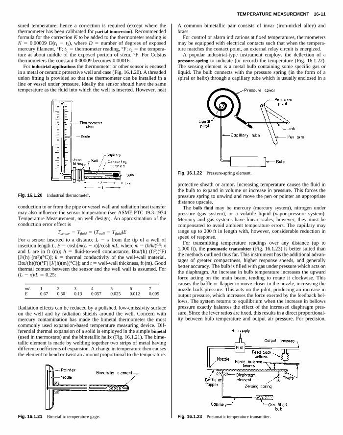
For industrial applications the thermometer or other sensor is encasedin a metal or ceramic protective well and case (Fig. 16.1.20). A threadedunion fitting is provided so that the thermometer can be installed in a
A common bimetallic pair consists of invar (iron-nickel alloy) andbrass.
For control or alarm indications at fixed temperatures, thermometersmay be equipped with electrical contacts such that when the tempera-ture matches the contact point, an external relay circuit is energized.
A popular industrial-type instrument employs the deflection of apressure-spring to indicate (or record) the temperature (Fig. 16.1.22).The sensing element is a metal bulb containing some specific gas orliquid. The bulb connects with the pressure spring (in the form of aspiral or helix) through a capillary tube which is usually enclosed in a
Copyright (C) 1999 by The McGraw-Hill Companies, Inc. All rights reserved. Use ofthis product is subject to the terms of its License Agreement. Click here to view.
line or vessel under pressure. Ideally the sensor should have the sametemperature as the fluid into which the well is inserted. However, heat
Fig. 16.1.20 Industrial thermometer.
conduction to or from the pipe or vessel wall and radiation heat transfermay also influence the sensor temperature (see ASME PTC 19.3-1974Temperature Measurement, on well design). An approximation of theconduction error effect is
Tsensor 2 Tfluid 5 (Twall 2 Tfluid)E
For a sensor inserted to a distance L 2 x from the tip of a well ofinsertion length L, E 5 cosh[m(L 2 x)]/cosh mL, where m 5 (h/kt)0.5; xand L are in ft (m); h 5 fluid-to-well conductance, Btu/(h) (ft2)(°F)[J/(h) (m2)(°C)]; k 5 thermal conductivity of the well-wall material.Btu/(h)(ft)(°F) [J/(h)(m)(°C)]; and t 5 well-wall thickness, ft (m). Goodthermal contact between the sensor and the well wall is assumed. For(L 2 x)/L 5 0.25:
mL 1 2 3 4 5 6 7E 0.67 0.30 0.13 0.057 0.025 0.012 0.005
Radiation effects can be reduced by a polished, low-emissivity surfaceon the well and by radiation shields around the well. Concern withmercury contamination has made the bimetal thermometer the mostcommonly used expansion-based temperature measuring device. Dif-ferential thermal expansion of a solid is employed in the simple bimetal(used in thermostats) and the bimetallic helix (Fig. 16.1.21). The bime-tallic element is made by welding together two strips of metal havingdifferent coefficients of expansion. A change in temperature then causesthe element to bend or twist an amount proportional to the temperature.
Fig. 16.1.21 Bimetallic temperature gage.
Fig. 16.1.22 Pressure-spring element.
protective sheath or armor. Increasing temperature causes the fluid inthe bulb to expand in volume or increase in pressure. This forces thepressure spring to unwind and move the pen or pointer an appropriatedistance upscale.
The bulb fluid may be mercury (mercury system), nitrogen underpressure (gas system), or a volatile liquid (vapor-pressure system).Mercury and gas systems have linear scales; however, they must becompensated to avoid ambient temperature errors. The capillary mayrange up to 200 ft in length with, however, considerable reduction inspeed of response.
For transmitting temperature readings over any distance (up to1,000 ft), the pneumatic transmitter (Fig. 16.1.23) is better suited thanthe methods outlined thus far. This instrument has the additional advan-tages of greater compactness, higher response speeds, and generallybetter accuracy. The bulb is filled with gas under pressure which acts onthe diaphragm. An increase in bulb temperature increases the upwardforce acting on the main beam, tending to rotate it clockwise. Thiscauses the baffle or flapper to move closer to the nozzle, increasing thenozzle back pressure. This acts on the pilot, producing an increase inoutput pressure, which increases the force exerted by the feedback bel-lows. The system returns to equilibrium when the increase in bellowspressure exactly balances the effect of the increased diaphragm pres-sure. Since the lever ratios are fixed, this results in a direct proportional-ity between bulb temperature and output air pressure. For precision,
Fig. 16.1.23 Pneumatic temperature transmitter.
16-12 INSTRUMENTS
compensating elements are built into the instrument to correct for theeffects of changes in barometric pressure and ambient temperature.
Electrical systems based on the thermocouple or resistance thermome-ter are particularly applicable where many different temperatures are tobe measured, where transmission distances are large, or where highsensitivity and rapid response are required. The thermocouple is usedwith high temperatures; the resistance thermometer for low tempera-tures and high accuracy requirements.
The choice of thermocouple depends on the temperature range, desiredaccuracy, and the nature of the atmosphere to which it is to be exposed.
mocouple voltage to temperature nonlinearities being stored in and ap-plied to the analog-to-digital converter (A/D) by a read-only memory(ROM) chip.
The resistance thermometer employs the same circuitry as describedabove, with the resistance element (RTD) being placed external to theinstrument and the cold junction being omitted (Fig. 16.1.26). Threetypes of RTD connections are in use: two wire, three wire, and fourwire. The two-wire connection makes the measurement sensitive to lead
20
8°CF (1F (2F (2F (2
1
Copyright (C) 1999 by The McGraw-Hill Companies, Inc. All rights reserved. Use ofthis product is subject to the terms of its License Agreement. Click here to view.
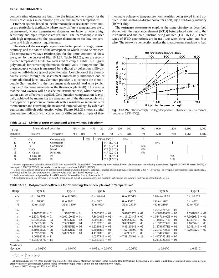
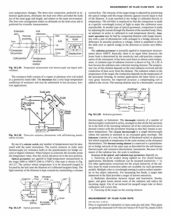
The temperature-voltage relationships for the more common of theseare given by the curves of Fig. 16.1.24. Table 16.1.2 gives the recom-mended temperature limits, for each kind of couple. Table 16.1.3 givespolynomials for converting thermocouple millivolts to temperature. Thethermocouple voltage is measured by a digital or deflection millivolt-meter or null-balance type of potentiometer. Completion of the thermo-couple circuit through the instrument immediately introduces one ormore additional junctions. Common practice is to connect the thermo-couple (hot junction) to the instrument with special lead wire (whichmay be of the same materials as the thermocouple itself). This assuresthat the cold junction will be inside the instrument case, where compen-sation can be effectively applied. Cold junction compensation is typi-cally achieved by measuring the temperature of the thermocouple wireto copper wire junctions or terminals with a resistive or semiconductorthermometer and correcting the measured terminal voltage by a derivedequivalent millivolt cold junction value. Figure 16.1.25 shows a digitaltemperature indicator with correction for different ANSI types of ther-
Table 16.1.2 Limits of Error on Standard Wires without Selection*†
Materials and polarities
Positive NegativeANSI
symbol‡
°F: 2 150 2 75 32
°C: 2 101 2 59 0
T Cu Constantan§ 2% 1.5°F (0.E Ni-Cr Constantan 3°J Fe Constantan 4°
K Ni-Cr Ni-Al 4°N Ni-Cr-Si Ni-SiMn 4°
R Pt-13% Rh Pt 3°F (1S Pt-10% Rh Pt 3°F (1* Protect copper from oxidation above 600°F; iron above 900°F. Protect Ni-Al from reducing atmused up to 3,200°F(1,700°C). Its standard error is 1⁄2 percent above 1,470°F (800°C).
† Closer tolerances are obtainable by selection and calibration. Consult makers’ catalogs. TungstenReference Tables for Low-Temperature Thermocouples. Natl. Bur. Stand. Monogr. 124.
‡ Individual wires are designated by the ANSI symbol followed by P or N; thus iron is JP.§ Constantan is 55% Cu, 45% Ni. The nickel-chromium and nickel-aluminum alloys are available
Table 16.1.3 Polynomial Coefficients for Converting Thermocouple emf
Range Type E Type J Type K
mV 0 to 76.373 0 to 42.919 0 to 20.644
°C 0 to 1000° 0 to 760° 0 to 500°°F 32 to 1832° 32 to 1400° 32 to 932°
a0 0 0 0a1 1.7057035E 1 01 1.978425E 1 01 2.508355E 1 01a2 2 2.3301759E 2 01 2 2.001204E 2 01 7.860106E 2 02a3 6.5435585E 2 03 1.036969E 2 02 2 2.503131E 2 01a4 2 7.3562749E 2 05 2 2.549687E 2 04 8.315270E 2 02a5 2 1.7896001E 2 06 3.585153E 2 06 2 1.228034E 2 02a6 8.4036165E 2 08 2 5.344285E 2 08 9.804036E 2 04a7 2 1.3735879E 2 09 5.099890E 2 10 2 4.413030E 2 05a8 1.0629823E 2 11 1.057734E 2 06a9 2 3.2447087E 2 14 2 1.052755E 2 08
Maximumdeviation 6 0.02°C 6 0.04°C 2 0.05 to 1 0.04°
* T (°C) 5 Oni 5 0
ai 3 (mV )i
All temperatures are ITS-1990 and all voltages are SI-1990 values. Maximum deviation is that frgreatly outside of given ranges. Consult source for thermocouple types B and R and for other milliv
SOURCE: NIST Monograph 175, April 1993.
Fig. 16.1.24 Thermocouple voltage-temperature characteristics [referencejunction at 32°F (0°C)].
0 530 600 700 1,000 1,400 2,300 2,700
93 277 316 371 538 760 1,260 1,482
) 3⁄4%.7°C) 1⁄2%.2°C) 3⁄4%.2°C) 3⁄4%.2°C) 3⁄4%
.5°C) ⁄4%.5°C) 1⁄4%ospheres. Protect platinum from nonreducing atmospheres. Type B (Pt-30% Rh versus Pt-6%) is
-rhenium alloys are in use up to 5,000°F (2,760°C). For cryogenic thermocouples see Sparks et al.,
as Chromel and Alumel, trademarks of Hoskins Mfg. Co.
to Temperature*
Type N Type S Type T
0 to 47.513 1.874 to 11.95 0 to 20.872
0 to 1300° 250 to 1200° 0 to 400°32 to 2372° 482 to 2192° 32 to 752°
0 1.291507177E 1 01 03.8783277E 1 01 1.466298863E 1 02 2.592800E 1 01
2 1.1612344E 1 00 2 1.534713402E 1 01 2 7.602961E 2 016.9525655E 2 02 3.145945973E 1 00 4.637791E 2 02
2 3.0090077E 2 03 2 4.163257839E 2 01 2 2.165394E 2 038.8311584E 2 05 3.187963771E 2 02 6.048144E 2 05
2 1.6213839E 2 06 2 1.291637500E 2 03 2 7.293422E 2 071.6693362E 2 08 2.183475087E 2 05
2 7.3117540E 2 11 2 1.447379511E 2 078.211272125E 2 09
C 6 0.06°C 6 0.01°C 6 0.03°C
om the ITS-1990 tables; thermocouple wire error is additional. Computed temperature deviatesolt ranges.
MEASUREMENT OF FLUID FLOW RATE 16-13
wire temperature changes. The three-wire connection, preferred in in-dustrial applications, eliminates the lead wire effect provided the leadsare of the same gage and length, and subject to the same environment.The four-wire arrangement makes no demands on the lead wires and ispreferred for scientific measurements.
LinearizationROM
Ref.
Voltreference
Thermalproximity
Extensionwire
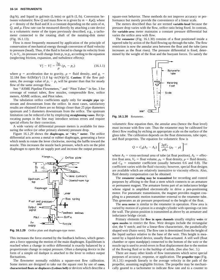
current flow. The intensity of the target image is adjusted by positioningthe optical wedge until the image intensity appears exactly equal to thatof the filament. A scale attached to the wedge is calibrated directly intemperature. The red filter is employed so that the comparison is madeat a specific wavelength (color) of light to make the calibration morereproducible. In another type of optical pyrometer, comparison is madeby adjusting the current through the filament of the standard lamp. Here,an ammeter in series is calibrated to read temperature directly. Auto-matic operation may be had by comparing filament with image intensi-ties with a pair of photoelectric cells arranged in a bridge network. A
Copyright (C) 1999 by The McGraw-Hill Companies, Inc. All rights reserved. Use ofthis product is subject to the terms of its License Agreement. Click here to view.
Iron A/D
(2)Display driver
converter
1In
Com.
Pre-amp.
T
Temperaturesensitiveresistor
Cold junction
Constantanhot junction
Fig. 16.1.25 Temperature measurement with thermocouple and digital milli-voltmeter.
The resistance bulb consists of a copper or platinum wire coil sealedin a protective metal tube. The thermistor has a very large temperaturecoefficient of resistance and may be substituted in low-accuracy, low-cost applications.
Fig. 16.1.26 Three-wire resistance thermometer with self-balancing potenti-ometer recorder.
By use of a selector switch, any number of temperatures may be mea-sured with the same instrument. The switch connects in order eachthermocouple (or resistance bulb) to the potentiometer (or bridge cir-cuit) or digital voltmeter. When balance is achieved, the recorder printsthe temperature value, then the switch advances on to the next position.
Optical pyrometers are applied to high-temperature measurement inthe range 1000 to 5000°F (540 to 2760°C). One type is shown in Fig.16.1.27. The surface whose temperature is to be measured (target) isfocused by the lens onto the filament of a calibrated tungsten lamp. Thelight intensity of the filament is kept constant by maintaining a constant
Fig. 16.1.27 Optical pyrometer.
difference in intensity produces a voltage, which is amplified to drivethe slide wire or optical wedge in the direction to restore zero differ-ence.
The radiation pyrometer is normally applied to temperature measure-ments above 1000°F. Basically, there is no upper limit; however, thelower limit is determined by the sensitivity and cold-junction compen-sation of the instrument. It has been used down to almost room temper-ature. A common type of radiation receiver is shown in Fig. 16.1.28. Alens focuses the radiation onto a thermal sensing element. The tempera-ture rise of this element depends on the total radiation received and theconduction of heat away from the element. The radiation relates to thetemperature of the target; the conduction depends on the temperature ofthe pyrometer housing. In normal applications the latter factor is notvery great; however, for improved accuracy a compensating coil isadded to the circuit. The sensing element may be a thermopile, vacuum
Fig. 16.1.28 Radiation pyrometer.
thermocouple, or bolometer. The thermopile consists of a number ofthermocouples connected in series, arranged so that all the hot junctionslie in the field of the incoming radiation; all of the cold junctions are inthermal contact with the pyrometer housing so that they remain at am-bient temperature. The vacuum thermocouple is a single thermocouplewhose hot junction is enclosed in an evacuated glass envelope. Thebolometer consists of a very thin strip of blackened nickel or platinumfoil which responds to temperature in the same manner as the resistancethermometer. The thermal sensing element is connected to a potentiome-ter or bridge network of the same type as described for the self-balancethermocouple and resistance-thermometer instruments. Because of thenature of the radiation law, the scale is nonlinear.
Accuracy of the optical- and radiation-type pyrometers depends on:1. Emissivity of the surface being sighted on. For closed furnace
applications, blackbody conditions can be assumed (emissivity 5 1).For other applications corrections for the actual emissivity of the sur-face must be made (correction tables are available for each pyrometermodel). Multiple color or wavelength sensing is used to reduce sensitiv-ity to hot object emissivity. For measuring hot fluids, a target tubeimmersed in the fluid provides a target of known emissivity.
2. Radiation absorption between target and instrument. Smoke,gases, and glass lenses absorb some of the radiation and reduce theincoming signal. Use of an enclosed (or purged) target tube or directcalibration will correct this.
3. Focusing of the target on the sensing element.
MEASUREMENT OF FLUID FLOW RATE(See also Secs. 3 and 4.)
Flow is expressed in volumetric or mass units per unit time. Thus gasesare generally measured in ft3/min (m3/min) or ft3/h (m3/h), steam in lb/h
16-14 INSTRUMENTS
(kg/h), and liquid in gal/min (L/min) or gal/h (L/h). Conversion be-tween volumetric flow Q and mass flow m is given by m 5 KrQ, wherer 5 density of the fluid and K is a constant depending on the units of m,Q, and r. Flow rate can be measured directly by attaching a rate deviceto a volumetric meter of the types previously described, e.g., a tacho-meter connected to the rotating shaft of the nutating-disk meter(Fig. 16.1.13).
Flow is most frequently measured by application of the principle ofconservation of mechanical energy through conversion of fluid velocityto pressure (head). Thus, if the fluid is forced to change its velocity from
square-root behavior. These methods do not improve accuracy or per-formance but merely provide the convenience of a linear scale.
The meters described thus far are termed variable-head because thepressure drop varies with the flow, orifice ratio being fixed. In contrast,the variable-area meter maintains a constant pressure differential butvaries the orifice area with flow.
The rotameter (Fig. 16.1.30) consists of a float positioned inside atapered tube by action of the fluid flowing up through the tube. The flowrestriction is now the annular area between the float and the tube (areaincreases as the float rises). The pressure differential is fixed, deter-
Copyright (C) 1999 by The McGraw-Hill Companies, Inc. All rights reserved. Use ofthis product is subject to the terms of its License Agreement. Click here to view.
V1 to V2 , its pressure will change from p1 to p2 according to the equation(neglecting friction, expansion, and turbulence effects):
V22 2 V1
2 52gc
r(p1 2 p2 ) (16.1.1)
where g 5 acceleration due to gravity, r 5 fluid density, and gc 532.184 lbm ? ft/(lbf)(s2) [1.0 kg ?m/(N)(s2)]. Caution: If the flow pul-sates, the average value of p1 2 p2 will be greater than that for steadyflow of the same average flow.
See ‘‘ASME Pipeline Flowmeters,’’ and ‘‘Pitot Tubes’’ in Sec. 3 forcoverage of venturi tubes, flow nozzles, compressible flow, orificemeters, ASME orifices, and Pitot tubes.
The tabulation orifice coefficients apply only for straight pipe up-stream and downstream from the orifice. In most cases, satisfactoryresults are obtained if there are no fittings closer than 25 pipe diametersupstream and 5 diameters downstream from the orifice. The upstreamlimitation can be reduced a bit by employing straightening vanes. Recip-rocating pumps in the line may introduce serious errors and requirespecial efforts for their correction.
A wide variety of differential pressure meters is available for mea-suring the orifice (or other primary element) pressure drop.
Figure 16.1.29 shows the diaphragm, or ‘‘dry,’’ meter. The orificedifferential acts across a metal or rubber diaphragm, generating a forcewhich tends to rotate the lever clockwise, moving the baffle toward thenozzle. This increases the nozzle back pressure, which acts on the pilotdiaphragm to open the air supply port and increase the output pressure.
Fig. 16.1.29 Orifice plate and diaphragm-type meter.
This increases the force exerted by the feedback bellows, which gener-ates a force opposing the motion of the main diaphragm. Equilibrium isreached when a change in orifice differential is exactly balanced by aproportionate change in output pressure. Often a damping device in theform of a simple oil dashpot is attached to the lever to reduce outputfluctuations.
The flowmeter normally exhibits a square-root flow calibration.Some meters are designed to take out the square root by use of cams,characterized floats or displacers (Ledoux bell) or devices which describe a
mined by the weight of the float and the buoyant forces. To satisfy the
Fig. 16.1.30 Rotameter.
volumetric flow equation then, the annular area (hence the float level)must increase with flow rate. Thus the rotameter may be calibrated fordirect flow reading by etching an appropriate scale on the surface of theglass tube. The calibration depends on the float dimensions, tube taper,and fluid properties. The equation for volumetric flow is
Q 5 CR(AT 2 AF) F2gVF
rAF
(rF 2 r)G1/2
where AT 5 cross-sectional area of tube (at float position), AF 5 effec-tive float area, VF 5 float volume, rF 5 float density, r 5 fluid density,and CR 5 rotameter coefficient (usually between 0.6 and 0.8). Thecoefficient varies with the fluid viscosity; however, special float designsare available which are relatively insensitive to viscosity effects. Also,fluid density compensation can be obtained.
The rotameter reading may be transmitted for recording and controlpurposes by affixing to the float a stem which connects to an armatureor permanent magnet. The armature forms part of an inductance bridgewhose signal is amplified electronically to drive a pen-positioningmotor. For pneumatic transmission, the magnet provides magnet cou-pling to a pneumatic motion transmitter external to the rotameter tube.This generates an air pressure proportional to the height of the float.
The area meter is similar to the rotameter in operation. Flow area isvaried by motion of a piston in a straight cylinder with openings cut intothe wall. The piston position is transmitted as above by an armature andinductance bridge circuit.
Primary elements for flow in open channels usually employ weirs oropen nozzles to restrict the flow. Weir designs include the rectangularslot; the V notch; and for a linear-flow characteristic, the parabolicallyshaped weir (Sutro weir). The flow rate is determined from the height ofthe liquid surface relative to the base of the weir. This height is mea-sured by a liquid-level device, usually float-actuated. A still well (floatchamber or open standpipe) connected to the bottom of the weir or thenozzle tap is used to avoid errors in float displacement due to the motionof the flowing fluid or to the buildup of solids. (See also Sec. 3.)
There are many other kinds of flow instruments which serve specialpurposes of accuracy, response, or application. The propeller type (Fig.16.1.31) responds linearly to the average velocity in the path of thepropeller, assuming negligible friction. The propeller may be mechani-cally geared to a tachometer to indicate flow rate and to a counter to
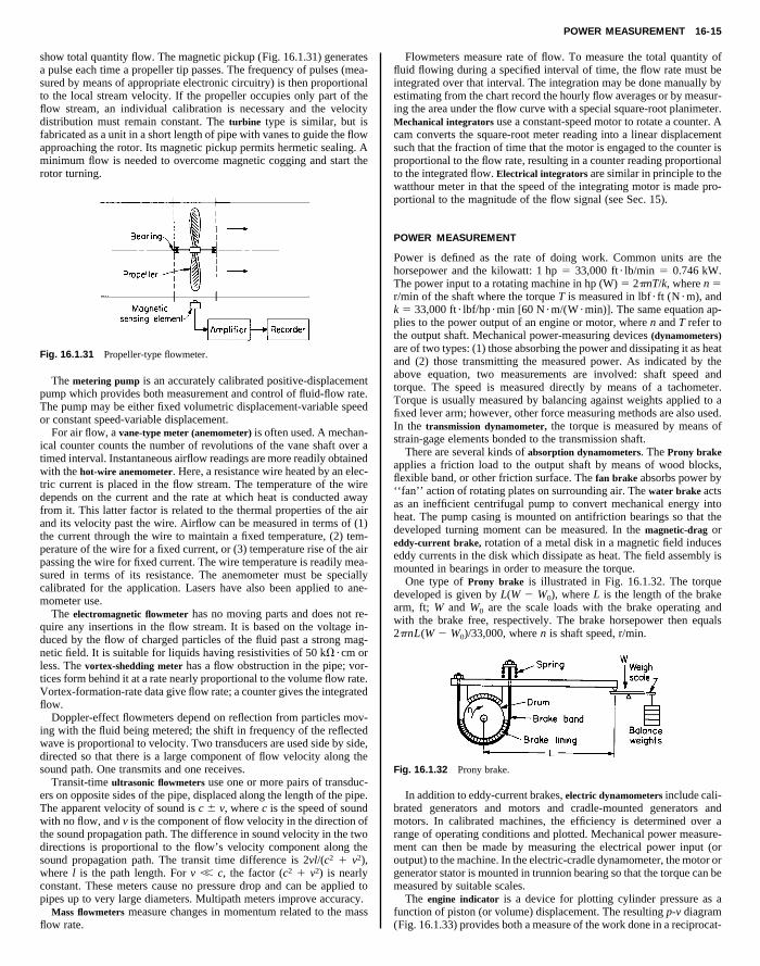
POWER MEASUREMENT 16-15
show total quantity flow. The magnetic pickup (Fig. 16.1.31) generatesa pulse each time a propeller tip passes. The frequency of pulses (mea-sured by means of appropriate electronic circuitry) is then proportionalto the local stream velocity. If the propeller occupies only part of theflow stream, an individual calibration is necessary and the velocitydistribution must remain constant. The turbine type is similar, but isfabricated as a unit in a short length of pipe with vanes to guide the flowapproaching the rotor. Its magnetic pickup permits hermetic sealing. Aminimum flow is needed to overcome magnetic cogging and start therotor turning.
Flowmeters measure rate of flow. To measure the total quantity offluid flowing during a specified interval of time, the flow rate must beintegrated over that interval. The integration may be done manually byestimating from the chart record the hourly flow averages or by measur-ing the area under the flow curve with a special square-root planimeter.Mechanical integrators use a constant-speed motor to rotate a counter. Acam converts the square-root meter reading into a linear displacementsuch that the fraction of time that the motor is engaged to the counter isproportional to the flow rate, resulting in a counter reading proportionalto the integrated flow. Electrical integrators are similar in principle to the
Copyright (C) 1999 by The McGraw-Hill Companies, Inc. All rights reserved. Use ofthis product is subject to the terms of its License Agreement. Click here to view.
Fig. 16.1.31 Propeller-type flowmeter.
The metering pump is an accurately calibrated positive-displacementpump which provides both measurement and control of fluid-flow rate.The pump may be either fixed volumetric displacement-variable speedor constant speed-variable displacement.
For air flow, a vane-type meter (anemometer) is often used. A mechan-ical counter counts the number of revolutions of the vane shaft over atimed interval. Instantaneous airflow readings are more readily obtainedwith the hot-wire anemometer. Here, a resistance wire heated by an elec-tric current is placed in the flow stream. The temperature of the wiredepends on the current and the rate at which heat is conducted awayfrom it. This latter factor is related to the thermal properties of the airand its velocity past the wire. Airflow can be measured in terms of (1)the current through the wire to maintain a fixed temperature, (2) tem-perature of the wire for a fixed current, or (3) temperature rise of the airpassing the wire for fixed current. The wire temperature is readily mea-sured in terms of its resistance. The anemometer must be speciallycalibrated for the application. Lasers have also been applied to ane-mometer use.
The electromagnetic flowmeter has no moving parts and does not re-quire any insertions in the flow stream. It is based on the voltage in-duced by the flow of charged particles of the fluid past a strong mag-netic field. It is suitable for liquids having resistivities of 50 kV?cm orless. The vortex-shedding meter has a flow obstruction in the pipe; vor-tices form behind it at a rate nearly proportional to the volume flow rate.Vortex-formation-rate data give flow rate; a counter gives the integratedflow.
Doppler-effect flowmeters depend on reflection from particles mov-ing with the fluid being metered; the shift in frequency of the reflectedwave is proportional to velocity. Two transducers are used side by side,directed so that there is a large component of flow velocity along thesound path. One transmits and one receives.
Transit-time ultrasonic flowmeters use one or more pairs of transduc-ers on opposite sides of the pipe, displaced along the length of the pipe.The apparent velocity of sound is c 6 v, where c is the speed of soundwith no flow, and v is the component of flow velocity in the direction ofthe sound propagation path. The difference in sound velocity in the twodirections is proportional to the flow’s velocity component along thesound propagation path. The transit time difference is 2vl/(c2 1 v2),where l is the path length. For v ,, c, the factor (c2 1 v2) is nearlyconstant. These meters cause no pressure drop and can be applied topipes up to very large diameters. Multipath meters improve accuracy.
Mass flowmeters measure changes in momentum related to the massflow rate.
watthour meter in that the speed of the integrating motor is made pro-portional to the magnitude of the flow signal (see Sec. 15).
POWER MEASUREMENT
Power is defined as the rate of doing work. Common units are thehorsepower and the kilowatt: 1 hp 5 33,000 ft ? lb/min 5 0.746 kW.The power input to a rotating machine in hp (W) 5 2pnT/k, where n 5r/min of the shaft where the torque T is measured in lbf ? ft (N ?m), andk 5 33,000 ft ? lbf/hp ?min [60 N ?m/(W ?min)]. The same equation ap-plies to the power output of an engine or motor, where n and T refer tothe output shaft. Mechanical power-measuring devices (dynamometers)are of two types: (1) those absorbing the power and dissipating it as heatand (2) those transmitting the measured power. As indicated by theabove equation, two measurements are involved: shaft speed andtorque. The speed is measured directly by means of a tachometer.Torque is usually measured by balancing against weights applied to afixed lever arm; however, other force measuring methods are also used.In the transmission dynamometer, the torque is measured by means ofstrain-gage elements bonded to the transmission shaft.
There are several kinds of absorption dynamometers. The Prony brakeapplies a friction load to the output shaft by means of wood blocks,flexible band, or other friction surface. The fan brake absorbs power by‘‘fan’’ action of rotating plates on surrounding air. The water brake actsas an inefficient centrifugal pump to convert mechanical energy intoheat. The pump casing is mounted on antifriction bearings so that thedeveloped turning moment can be measured. In the magnetic-drag oreddy-current brake, rotation of a metal disk in a magnetic field induceseddy currents in the disk which dissipate as heat. The field assembly ismounted in bearings in order to measure the torque.
One type of Prony brake is illustrated in Fig. 16.1.32. The torquedeveloped is given by L(W 2 W0), where L is the length of the brakearm, ft; W and W0 are the scale loads with the brake operating andwith the brake free, respectively. The brake horsepower then equals2pnL(W 2 W0)/33,000, where n is shaft speed, r/min.
Fig. 16.1.32 Prony brake.
In addition to eddy-current brakes, electric dynamometers include cali-brated generators and motors and cradle-mounted generators andmotors. In calibrated machines, the efficiency is determined over arange of operating conditions and plotted. Mechanical power measure-ment can then be made by measuring the electrical power input (oroutput) to the machine. In the electric-cradle dynamometer, the motor orgenerator stator is mounted in trunnion bearing so that the torque can bemeasured by suitable scales.
The engine indicator is a device for plotting cylinder pressure as afunction of piston (or volume) displacement. The resulting p-v diagram(Fig. 16.1.33) provides both a measure of the work done in a reciprocat-
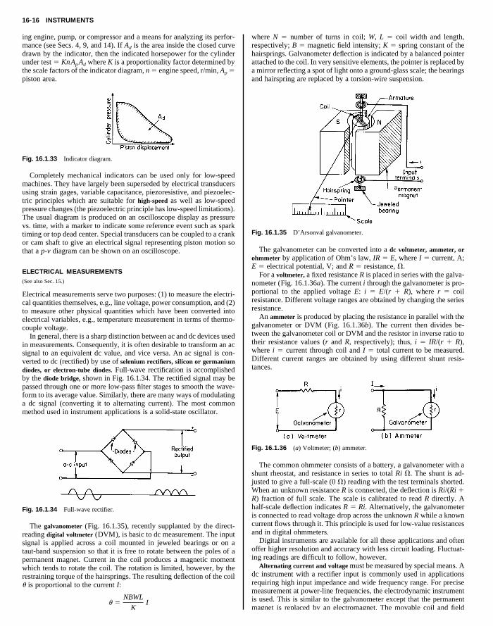
16-16 INSTRUMENTS
ing engine, pump, or compressor and a means for analyzing its perfor-mance (see Secs. 4, 9, and 14). If Ad is the area inside the closed curvedrawn by the indicator, then the indicated horsepower for the cylinderunder test 5 KnApAd where K is a proportionality factor determined bythe scale factors of the indicator diagram, n 5 engine speed, r/min, Ap 5piston area.
where N 5 number of turns in coil; W, L 5 coil width and length,respectively; B 5 magnetic field intensity; K 5 spring constant of thehairsprings. Galvanometer deflection is indicated by a balanced pointerattached to the coil. In very sensitive elements, the pointer is replaced bya mirror reflecting a spot of light onto a ground-glass scale; the bearingsand hairspring are replaced by a torsion-wire suspension.
Copyright (C) 1999 by The McGraw-Hill Companies, Inc. All rights reserved. Use ofthis product is subject to the terms of its License Agreement. Click here to view.
Fig. 16.1.33 Indicator diagram.
Completely mechanical indicators can be used only for low-speedmachines. They have largely been superseded by electrical transducersusing strain gages, variable capacitance, piezoresistive, and piezoelec-tric principles which are suitable for high-speed as well as low-speedpressure changes (the piezoelectric principle has low-speed limitations).The usual diagram is produced on an oscilloscope display as pressurevs. time, with a marker to indicate some reference event such as sparktiming or top dead center. Special transducers can be coupled to a crankor cam shaft to give an electrical signal representing piston motion sothat a p-v diagram can be shown on an oscilloscope.
ELECTRICAL MEASUREMENTS(See also Sec. 15.)
Electrical measurements serve two purposes: (1) to measure the electri-cal quantities themselves, e.g., line voltage, power consumption, and (2)to measure other physical quantities which have been converted intoelectrical variables, e.g., temperature measurement in terms of thermo-couple voltage.
In general, there is a sharp distinction between ac and dc devices usedin measurements. Consequently, it is often desirable to transform an acsignal to an equivalent dc value, and vice versa. An ac signal is con-verted to dc (rectified) by use of selenium rectifiers, silicon or germaniumdiodes, or electron-tube diodes. Full-wave rectification is accomplishedby the diode bridge, shown in Fig. 16.1.34. The rectified signal may bepassed through one or more low-pass filter stages to smooth the wave-form to its average value. Similarly, there are many ways of modulatinga dc signal (converting it to alternating current). The most commonmethod used in instrument applications is a solid-state oscillator.
Fig. 16.1.34 Full-wave rectifier.
The galvanometer (Fig. 16.1.35), recently supplanted by the direct-reading digital voltmeter (DVM), is basic to dc measurement. The inputsignal is applied across a coil mounted in jeweled bearings or on ataut-band suspension so that it is free to rotate between the poles of apermanent magnet. Current in the coil produces a magnetic momentwhich tends to rotate the coil. The rotation is limited, however, by therestraining torque of the hairsprings. The resulting deflection of the coilu is proportional to the current I:
u 5NBWL
KI
Fig. 16.1.35 D’Arsonval galvanometer.
The galvanometer can be converted into a dc voltmeter, ammeter, orohmmeter by application of Ohm’s law, IR 5 E, where I 5 current, A;E 5 electrical potential, V; and R 5 resistance, V.
For a voltmeter, a fixed resistance R is placed in series with the galva-nometer (Fig. 16.1.36a). The current i through the galvanometer is pro-portional to the applied voltage E: i 5 E/(r 1 R), where r 5 coilresistance. Different voltage ranges are obtained by changing the seriesresistance.
An ammeter is produced by placing the resistance in parallel with thegalvanometer or DVM (Fig. 16.1.36b). The current then divides be-tween the galvanometer coil or DVM and the resistor in inverse ratio totheir resistance values (r and R, respectively); thus, i 5 IR/(r 1 R),where i 5 current through coil and I 5 total current to be measured.Different current ranges are obtained by using different shunt resis-tances.
Fig. 16.1.36 (a) Voltmeter; (b) ammeter.
The common ohmmeter consists of a battery, a galvanometer with ashunt rheostat, and resistance in series to total Ri V. The shunt is ad-justed to give a full-scale (0 V) reading with the test terminals shorted.When an unknown resistance R is connected, the deflection is Ri/(Ri 1R) fraction of full scale. The scale is calibrated to read R directly. Ahalf-scale deflection indicates R 5 Ri. Alternatively, the galvanometeris connected to read voltage drop across the unknown R while a knowncurrent flows through it. This principle is used for low-value resistancesand in digital ohmmeters.
Digital instruments are available for all these applications and oftenoffer higher resolution and accuracy with less circuit loading. Fluctuat-ing readings are difficult to follow, however.
Alternating current and voltage must be measured by special means. Adc instrument with a rectifier input is commonly used in applicationsrequiring high input impedance and wide frequency range. For precisemeasurement at power-line frequencies, the electrodynamic instrumentis used. This is similar to the galvanometer except that the permanentmagnet is replaced by an electromagnet. The movable coil and field
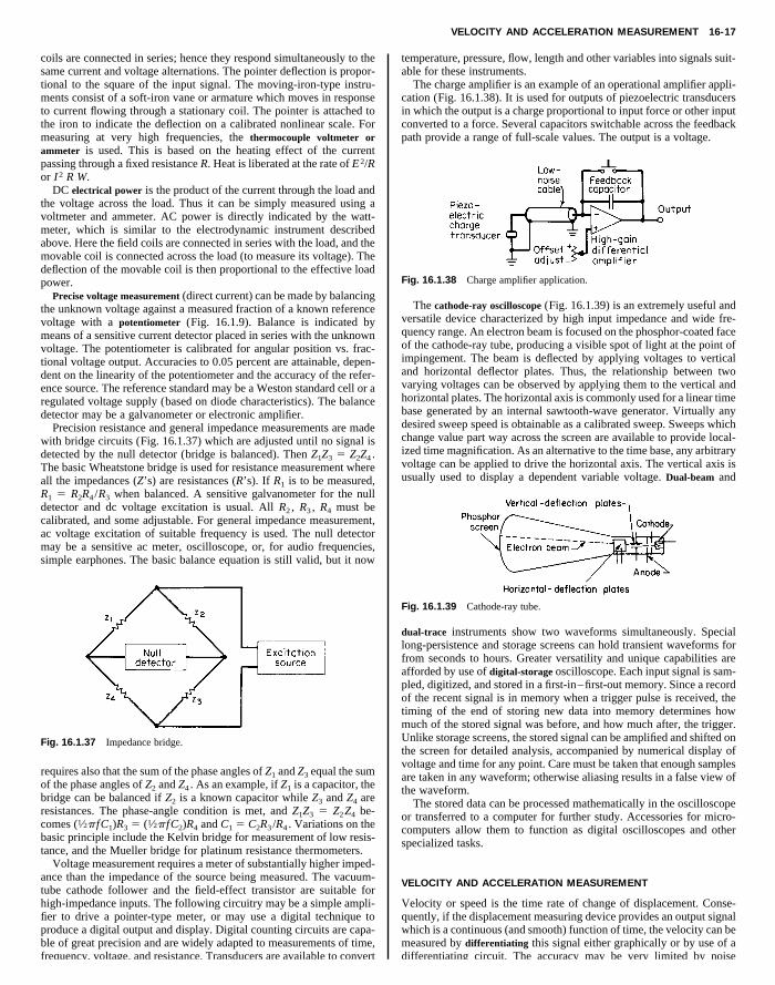
VELOCITY AND ACCELERATION MEASUREMENT 16-17
coils are connected in series; hence they respond simultaneously to thesame current and voltage alternations. The pointer deflection is propor-tional to the square of the input signal. The moving-iron-type instru-ments consist of a soft-iron vane or armature which moves in responseto current flowing through a stationary coil. The pointer is attached tothe iron to indicate the deflection on a calibrated nonlinear scale. Formeasuring at very high frequencies, the thermocouple voltmeter orammeter is used. This is based on the heating effect of the currentpassing through a fixed resistance R. Heat is liberated at the rate of E2/Ror I2 R W.
temperature, pressure, flow, length and other variables into signals suit-able for these instruments.
The charge amplifier is an example of an operational amplifier appli-cation (Fig. 16.1.38). It is used for outputs of piezoelectric transducersin which the output is a charge proportional to input force or other inputconverted to a force. Several capacitors switchable across the feedbackpath provide a range of full-scale values. The output is a voltage.
Copyright (C) 1999 by The McGraw-Hill Companies, Inc. All rights reserved. Use ofthis product is subject to the terms of its License Agreement. Click here to view.
DC electrical power is the product of the current through the load andthe voltage across the load. Thus it can be simply measured using avoltmeter and ammeter. AC power is directly indicated by the watt-meter, which is similar to the electrodynamic instrument describedabove. Here the field coils are connected in series with the load, and themovable coil is connected across the load (to measure its voltage). Thedeflection of the movable coil is then proportional to the effective loadpower.
Precise voltage measurement (direct current) can be made by balancingthe unknown voltage against a measured fraction of a known referencevoltage with a potentiometer (Fig. 16.1.9). Balance is indicated bymeans of a sensitive current detector placed in series with the unknownvoltage. The potentiometer is calibrated for angular position vs. frac-tional voltage output. Accuracies to 0.05 percent are attainable, depen-dent on the linearity of the potentiometer and the accuracy of the refer-ence source. The reference standard may be a Weston standard cell or aregulated voltage supply (based on diode characteristics). The balancedetector may be a galvanometer or electronic amplifier.
Precision resistance and general impedance measurements are madewith bridge circuits (Fig. 16.1.37) which are adjusted until no signal isdetected by the null detector (bridge is balanced). Then Z1Z3 5 Z2Z4 .The basic Wheatstone bridge is used for resistance measurement whereall the impedances (Z’s) are resistances (R’s). If R1 is to be measured,R1 5 R2R4 /R3 when balanced. A sensitive galvanometer for the nulldetector and dc voltage excitation is usual. All R2 , R3 , R4 must becalibrated, and some adjustable. For general impedance measurement,ac voltage excitation of suitable frequency is used. The null detectormay be a sensitive ac meter, oscilloscope, or, for audio frequencies,simple earphones. The basic balance equation is still valid, but it now
Fig. 16.1.37 Impedance bridge.
requires also that the sum of the phase angles of Z1 and Z3 equal the sumof the phase angles of Z2 and Z4 . As an example, if Z1 is a capacitor, thebridge can be balanced if Z2 is a known capacitor while Z3 and Z4 areresistances. The phase-angle condition is met, and Z1Z3 5 Z2Z4 be-comes (1⁄2p fC1)R3 5 (1⁄2p fC2)R4 and C1 5 C2R3 /R4 . Variations on thebasic principle include the Kelvin bridge for measurement of low resis-tance, and the Mueller bridge for platinum resistance thermometers.
Voltage measurement requires a meter of substantially higher imped-ance than the impedance of the source being measured. The vacuum-tube cathode follower and the field-effect transistor are suitable forhigh-impedance inputs. The following circuitry may be a simple ampli-fier to drive a pointer-type meter, or may use a digital technique toproduce a digital output and display. Digital counting circuits are capa-ble of great precision and are widely adapted to measurements of time,frequency, voltage, and resistance. Transducers are available to convert
Fig. 16.1.38 Charge amplifier application.
The cathode-ray oscilloscope (Fig. 16.1.39) is an extremely useful andversatile device characterized by high input impedance and wide fre-quency range. An electron beam is focused on the phosphor-coated faceof the cathode-ray tube, producing a visible spot of light at the point ofimpingement. The beam is deflected by applying voltages to verticaland horizontal deflector plates. Thus, the relationship between twovarying voltages can be observed by applying them to the vertical andhorizontal plates. The horizontal axis is commonly used for a linear timebase generated by an internal sawtooth-wave generator. Virtually anydesired sweep speed is obtainable as a calibrated sweep. Sweeps whichchange value part way across the screen are available to provide local-ized time magnification. As an alternative to the time base, any arbitraryvoltage can be applied to drive the horizontal axis. The vertical axis isusually used to display a dependent variable voltage. Dual-beam and
Fig. 16.1.39 Cathode-ray tube.
dual-trace instruments show two waveforms simultaneously. Speciallong-persistence and storage screens can hold transient waveforms forfrom seconds to hours. Greater versatility and unique capabilities areafforded by use of digital-storage oscilloscope. Each input signal is sam-pled, digitized, and stored in a first-in–first-out memory. Since a recordof the recent signal is in memory when a trigger pulse is received, thetiming of the end of storing new data into memory determines howmuch of the stored signal was before, and how much after, the trigger.Unlike storage screens, the stored signal can be amplified and shifted onthe screen for detailed analysis, accompanied by numerical display ofvoltage and time for any point. Care must be taken that enough samplesare taken in any waveform; otherwise aliasing results in a false view ofthe waveform.
The stored data can be processed mathematically in the oscilloscopeor transferred to a computer for further study. Accessories for micro-computers allow them to function as digital oscilloscopes and otherspecialized tasks.
VELOCITY AND ACCELERATION MEASUREMENT
Velocity or speed is the time rate of change of displacement. Conse-quently, if the displacement measuring device provides an output signalwhich is a continuous (and smooth) function of time, the velocity can bemeasured by differentiating this signal either graphically or by use of adifferentiating circuit. The accuracy may be very limited by noise

16-18 INSTRUMENTS
(high-frequency fluctuations), however. More commonly, the output ofan accelerometer is integrated to yield the velocity of the moving mem-ber. Average speed over a time interval can be determined by measuringthe time required for the moving body to pass two fixed points a knowndistance apart. Here photoelectric or other rapid sensing devices may beused to trigger the start and stop of the timer. Rotational speed may besimilarly measured by counting the number of rotations in a fixed timeinterval.
The tachometer provides a direct measure of angular velocity. Oneform is essentially a small permanent-magnet-type generator coupled to
measurements: infrared absorption spectra, ultraviolet and visible emissionspectra, mass spectrometry, and gas chromatography. These are specific toparticular types of compounds and molecular configurations and henceare very powerful in the analysis of complex mixtures. As examples,infrared analyzers are in use to measure low-concentration contami-nants in engine oils resulting from wear and in hydraulic oils to detectdeterioration. X-ray diffraction has many applications in the analysis ofcrystalline solids, metals, and solid solutions.
Of special importance in the realm of composition measurements isthe determination of moisture content. A common laboratory procedure
the rotating element; the voltage induced in the armature coil is directlyproportional to the speed. The principle is also extended to rectilinearmotions (restricted to small displacements) by using a straight coilmoving in a fixed magnetic field.
Angular velocity can also be measured by magnetic drag-cup andcentrifugal-force devices (flyball governor). The force may be balancedagainst a spring with the resulting deflection calibrated in terms of theshaft speed. Alternatively, the force may be balanced against the airpressure generated by a pneumatic nozzle-baffle assembly (similar toFig. 16.1.23).
Vibration velocity pickups may use a coil which moves relative to amagnet. The voltage generated in the coil has the same frequency as thevibration and, for sine motion, a magnitude proportional to the productof vibration frequency and amplitude. Vibration acceleration pickupscommonly use strain-gage, piezoresistive, or piezoelectric elements tosense a force F 5 Ma/gc . The maximum usable frequency of an acce-lerometer is about one-fifth of the pickup’s natural frequency (see Sec.3.4). The minimum usable frequency depends on the type of pickup andthe associated circuitry. The output of an accelerometer can be inte-grated to obtain a velocity signal; a velocity signal can be integrated toobtain a displacement signal. The operational amplifier is a versatileelement which can be connected as an integrator for this use.
Holography is being applied to the study of surface vibration patterns.
MEASUREMENT OF PHYSICAL AND CHEMICALPROPERTIES
Physical and chemical measurements are important in the control ofproduct quality and composition. In the case of manufactured items,such properties as color, hardness, surface, roughness, etc., are of inter-est. Color is measured by means of a colorimeter, which provides com-parison with color standards, or by means of a spectrophotometer, whichanalyzes the color spectrum. The Brinell and Rockwell testers measuresurface hardness in terms of the depth of penetration of a hardened steelball or special stylus. Testing machines with strain-gage elements pro-vide measurement of the strength and elastic properties of materials.Profilometers are used to measure surface characteristics. In one type,the surface contour is magnified optically and the image projected ontoa screen or viewer; in another, a stylus is employed to translate thesurface irregularities into an electrical signal which may be recorded inthe form of a highly magnified profile of the surface or presented as anaveraged roughness-factor reading.
For liquids, attributes such as density, viscosity, melting point, boil-ing point, transparency, etc., are important. Density measurements havealready been discussed. Viscosity is measured with a viscosimeter, ofwhich there are three main types: flow through an orifice or capillary(Saybolt), viscous drag on a cylinder rotating in the fluid (MacMichael),damping of a vibrating reed (Ultrasonic) (see Secs. 3 and 4). Plasticityand consistency are related properties which are determined with spe-cial apparatus for heating or cooling the material and observing thetemperature-time curve. The photometer, reflectometer, and turbidimeterare devices for measuring transparency or turbidity of nonopaque liq-uids and solids.
A variety of properties can be measured for determining chemicalcomposition. Electrical properties include pH, conductivity, dielectricconstant, oxidation potential, etc. Physical properties include density,refractive index, thermal conductivity, vapor pressure, melting andboiling points, etc. Of increasing industrial application are spectroscopic
measures the loss of weight of the oven-dried sample. More rapid meth-ods employ electrical conductance or capacitance measurements, basedon the relatively high conductivity and dielectric constant values forordinary water.
Water vapor in air (humidity) is measured in terms of its physicalproperties or effects on materials (see also Secs. 4 and 12). (1) Thepsychrometer is based on the cooling effect of water evaporating into theairstream. It consists of two thermal elements exposed to a steady air-flow; one is dry, the other is kept moist. See Sec. 4 for psychrometriccharts. (2) The dew-point recorder measures the temperature at whichwater just starts to condense out of the air. (3) The hygrometer measuresthe change in length of such humidity-sensitive elements as hair andwood. (4) Electric sensing elements employ a wire-wound coil impreg-nated with a hygroscopic salt (one that maintains an equilibrium be-tween its moisture content and the air humidity) such that the resistanceof the coil is related to the humidity.
The throttling calorimeter (Fig. 16.1.40) is most commonly used fordetermining the moisture in steam. A sampling nozzle is located prefer-ably in a vertical section of steampipe far removed from any fittings.Steam enters the calorimeter through a throttling orifice and into a well-insulated expansion chamber. The steam quality x (fraction dry steam)is determined from the equation x 5 (hc 2 hf) / hfg , where hc is theenthalpy of superheated steam at the temperature and pressure measured
Fig. 16.1.40 Throttling calorimeter.
in the calorimeter; hf and hfg are, respectively, the liquid enthalpy andthe heat of vaporization corresponding to line pressure. The chamber isconveniently exhausted to atmospheric pressure; then only line pressureand temperature of the throttled steam need be measured. The range ofthe throttling calorimeter is limited to small percentages of moisture; aseparating calorimeter may be employed for larger moisture contents.
The Orsat apparatus is generally used for chemical analysis of fluegases. It consists of a graduated tube or burette designed to receive andmeasure volumes of gas (at constant temperature). The gas is analyzedfor CO2 , O2 , CO, and N2 by bubbling through appropriate absorbingreagents and measuring the resulting change in volume. The reagentsnormally employed are KOH solution for CO2, pyrogallic acid and
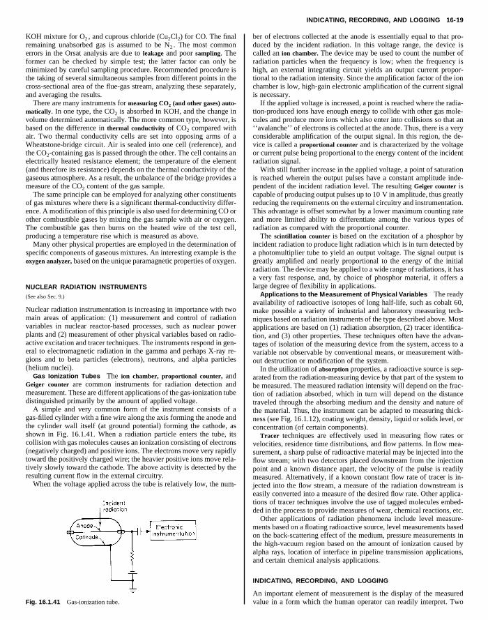
INDICATING, RECORDING, AND LOGGING 16-19
KOH mixture for O2 , and cuprous chloride (Cu2Cl2) for CO. The finalremaining unabsorbed gas is assumed to be N2 . The most commonerrors in the Orsat analysis are due to leakage and poor sampling. Theformer can be checked by simple test; the latter factor can only beminimized by careful sampling procedure. Recommended procedure isthe taking of several simultaneous samples from different points in thecross-sectional area of the flue-gas stream, analyzing these separately,and averaging the results.
There are many instruments for measuring CO2 (and other gases) auto-matically. In one type, the CO2 is absorbed in KOH, and the change in
ber of electrons collected at the anode is essentially equal to that pro-duced by the incident radiation. In this voltage range, the device iscalled an ion chamber. The device may be used to count the number ofradiation particles when the frequency is low; when the frequency ishigh, an external integrating circuit yields an output current propor-tional to the radiation intensity. Since the amplification factor of the ionchamber is low, high-gain electronic amplification of the current signalis necessary.
If the applied voltage is increased, a point is reached where the radia-tion-produced ions have enough energy to collide with other gas mole-
volume determined automatically. The more common type, however, isbased on the difference in thermal conductivity of CO2 compared withair. Two thermal conductivity cells are set into opposing arms of aWheatstone-bridge circuit. Air is sealed into one cell (reference), andthe CO2-containing gas is passed through the other. The cell contains anelectrically heated resistance element; the temperature of the element(and therefore its resistance) depends on the thermal conductivity of thegaseous atmosphere. As a result, the unbalance of the bridge provides ameasure of the CO2 content of the gas sample.
The same principle can be employed for analyzing other constituentsof gas mixtures where there is a significant thermal-conductivity differ-ence. A modification of this principle is also used for determining CO orother combustible gases by mixing the gas sample with air or oxygen.The combustible gas then burns on the heated wire of the test cell,producing a temperature rise which is measured as above.
Many other physical properties are employed in the determination ofspecific components of gaseous mixtures. An interesting example is theoxygen analyzer, based on the unique paramagnetic properties of oxygen.
NUCLEAR RADIATION INSTRUMENTS(See also Sec. 9.)
Nuclear radiation instrumentation is increasing in importance with twomain areas of application: (1) measurement and control of radiationvariables in nuclear reactor-based processes, such as nuclear powerplants and (2) measurement of other physical variables based on radio-active excitation and tracer techniques. The instruments respond in gen-eral to electromagnetic radiation in the gamma and perhaps X-ray re-gions and to beta particles (electrons), neutrons, and alpha particles(helium nuclei).
Gas Ionization Tubes The ion chamber, proportional counter, andGeiger counter are common instruments for radiation detection andmeasurement. These are different applications of the gas-ionization tubedistinguished primarily by the amount of applied voltage.
A simple and very common form of the instrument consists of agas-filled cylinder with a fine wire along the axis forming the anode andthe cylinder wall itself (at ground potential) forming the cathode, asshown in Fig. 16.1.41. When a radiation particle enters the tube, itscollision with gas molecules causes an ionization consisting of electrons(negatively charged) and positive ions. The electrons move very rapidlytoward the positively charged wire; the heavier positive ions move rela-tively slowly toward the cathode. The above activity is detected by theresulting current flow in the external circuitry.
When the voltage applied across the tube is relatively low, the num-
Fig. 16.1.41 Gas-ionization tube.
cules and produce more ions which also enter into collisions so that an‘‘avalanche’’ of electrons is collected at the anode. Thus, there is a veryconsiderable amplification of the output signal. In this region, the de-vice is called a proportional counter and is characterized by the voltageor current pulse being proportional to the energy content of the incidentradiation signal.
With still further increase in the applied voltage, a point of saturationis reached wherein the output pulses have a constant amplitude inde-pendent of the incident radiation level. The resulting Geiger counter iscapable of producing output pulses up to 10 V in amplitude, thus greatlyreducing the requirements on the external circuitry and instrumentation.This advantage is offset somewhat by a lower maximum counting rateand more limited ability to differentiate among the various types ofradiation as compared with the proportional counter.
The scintillation counter is based on the excitation of a phosphor byincident radiation to produce light radiation which is in turn detected bya photomultiplier tube to yield an output voltage. The signal output isgreatly amplified and nearly proportional to the energy of the initialradiation. The device may be applied to a wide range of radiations, it hasa very fast response, and, by choice of phosphor material, it offers alarge degree of flexibility in applications.
Applications to the Measurement of Physical Variables The readyavailability of radioactive isotopes of long half-life, such as cobalt 60,make possible a variety of industrial and laboratory measuring tech-niques based on radiation instruments of the type described above. Mostapplications are based on (1) radiation absorption, (2) tracer identifica-tion, and (3) other properties. These techniques often have the advan-tages of isolation of the measuring device from the system, access to avariable not observable by conventional means, or measurement with-out destruction or modification of the system.
In the utilization of absorption properties, a radioactive source is sep-arated from the radiation-measuring device by that part of the system tobe measured. The measured radiation intensity will depend on the frac-tion of radiation absorbed, which in turn will depend on the distancetraveled through the absorbing medium and the density and nature ofthe material. Thus, the instrument can be adapted to measuring thick-ness (see Fig. 16.1.12), coating weight, density, liquid or solids level, orconcentration (of certain components).
Tracer techniques are effectively used in measuring flow rates orvelocities, residence time distributions, and flow patterns. In flow mea-surement, a sharp pulse of radioactive material may be injected into theflow stream; with two detectors placed downstream from the injectionpoint and a known distance apart, the velocity of the pulse is readilymeasured. Alternatively, if a known constant flow rate of tracer is in-jected into the flow stream, a measure of the radiation downstream iseasily converted into a measure of the desired flow rate. Other applica-tions of tracer techniques involve the use of tagged molecules embed-ded in the process to provide measures of wear, chemical reactions, etc.
Other applications of radiation phenomena include level measure-ments based on a floating radioactive source, level measurements basedon the back-scattering effect of the medium, pressure measurements inthe high-vacuum region based on the amount of ionization caused byalpha rays, location of interface in pipeline transmission applications,and certain chemical analysis applications.
INDICATING, RECORDING, AND LOGGING
An important element of measurement is the display of the measuredvalue in a form which the human operator can readily interpret. Two
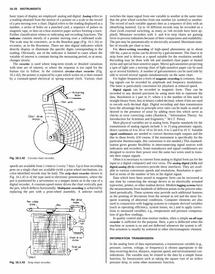
16-20 INSTRUMENTS
basic types of display are employed: analog and digital. Analog refers toa reading obtained from the motion of a pointer on a scale or the recordof a pen moving over a chart. Digital refers to the reading displayed as anumber, a series of holes on a punched card, a sequence of pulses onmagnetic tape, or dots on a heat sensitive paper surface forming a trace.Further classification relates to indicating and recording functions. Theindicator consists merely of a pointer moving over a calibrated scale.The scale may be concentric, as in the Bourdon gage (Fig. 16.1.16) oreccentric, as in the flowmeter. There are also digital indicators whichdirectly display or illuminate the specific digits corresponding to the
switches the input signal from one variable to another at the same timethat the print wheel switches from one number (or symbol) to another.The record of each variable appears then as a sequence of dots with anidentifying numeral. Up to 16 different records may be recorded on achart (with external switching, as many as 144 records have been ap-plied). Miniature recorders with 3- and 4-in strip charts are gainingfavor in process industries because of their compactness and readability.The pen may be pneumatically or electrically actuated. Maximum num-ber of records per chart is two.
For direct-writing recording of high-speed phenomena up to about
Copyright (C) 1999 by The McGraw-Hill Companies, Inc. All rights reserved. Use ofthis product is subject to the terms of its License Agreement. Click here to view.
reading. Obviously, use of the indicator is limited to cases where thevariable of interest is constant during the measuring period, or at most,changes slowly.
The recorder is used where long-term trends or detailed variationswith time are of interest, or where the response is too rapid for thehuman eye to follow. In the common circular-chart recorder (Fig.16.1.42), the pointer is replaced by a pen which writes on a chart rotatedby a constant-speed electrical or spring-wound clock. Various chart
Fig. 16.1.42 Circular-chart recorder.
speeds are available from 1 r/min to 1 every 7 days. Up to four recordingpens on a single chart are available (with a print-wheel mechanism, sixcolor-identified records may be had). The strip-chart recorder shown inFig. 16.1.43 is of the type used in electronic potentiometers, where thepen is positioned by a servomotor or a stepper motor as in the case of adigital recorder. A constant-speed motor drives the chart vertically pastthe pen, which deflects horizontally. Multipoint recording is achieved byreplacing the pen with a print-wheel assembly. A selector switch
Fig. 16.1.43 Strip-chart recorder.
100 Hz, a pen or stylus can be driven by a galvanometer. The chart is instrip form and is driven at a speed suitable for the resolution needed.Recording may be done with ink and standard chart paper or heatedstylus and special heat-sensitive paper. Mirror galvanometers projectinga spot of light onto a moving chart of light-sensitive paper can be usedup to several kilohertz. A number of galvanometers can be used side byside to record several signals simultaneously on the same chart.
For higher frequencies a form of magnetic recording is common. Ana-log signals can be recorded by amplitude and frequency modulation.The latter is particularly convenient for playback at reduced speed.
Digital signals can be recorded in magnetic form. They can berecorded to any desired precision by using more bits to represent thedata. Resolution is 1 part in 2n, where n is the number of bits used instraight binary form, less in binary-coded decimal, where 4 bits are usedto encode each decimal digit. Digital recording and data transmissionhave the advantage that in principle error rates can be made as small asdesired in the presence of noise by adding more bits which serve aschecks in error correcting codes (Raisbeck, ‘‘Information Theory: AnIntroduction for Scientists and Engineers,’’ M.I.T. Press).
Most physical variables are in analog form. Popular standards for thetransmission of analog signals include 3- to 15-psig pneumatic signals,direct currents of 4 to 20 or 10 to 50 mA, 0 to 5 and 0 to 10 V. Suitablesignal conditioners are needed to convert thermocouple outputs and thelike to these levels. (Of course, if the instrument is specifically for theparticular thermocouple, this conversion is not needed.) This standard-ization gives greater flexibility in interconnecting signal sources withindicators and recorders. Some transducers and signal conditioners aredesigned to receive their power over the same two wires used to trans-mit their output signals.
Often it is necessary to convert from analog to digital form (as for theinput to a digital computer) and vice versa. The analog-digital (A/D) anddigital-analog (D/A) converters provide these interfaces. They are avail-able in various conversion speeds and resolutions. Resolution is speci-fied in terms of the number of bits in the digital signal.
Data which have been stored in magnetic form can be recovered atany time by connecting the storage device to an electrically actuatedtypewriter, printer, or other readout device. Modern logging systems havethe measurements from hundreds of different points in the process tabu-lated periodically. These systems may provide such additional featuresas the printing of deviations from the normal in red and the more fre-quent scanning of abnormal conditions. Computer elements are alsoused in conjunction with logging systems to compute derived variables(such as operating efficiency, system losses, etc.) and to apply correc-tions to measured variables, e.g., temperature and pressure compensa-tion of gas-flow readings.
In quality control and time-motion studies, often a simple on-off-typerecorder is sufficient for the purpose. Here, a pen is deflected when themachine or system is on and not deflected whenever the system is off.Pen actuation is usually by solenoid or other electromagnetic element.
INFORMATION TRANSMISSION
In the analog form of data representation, a transmission variable (e.g.,pressure, current, voltage, or frequency) is chosen appropriate to thedata receiving device, distance, response speed, and environmental con-siderations. The variable may be related to the data by a simple linearfunction, by linearization such as taking the square root of an orificepressure drop, or some other monotonic function.
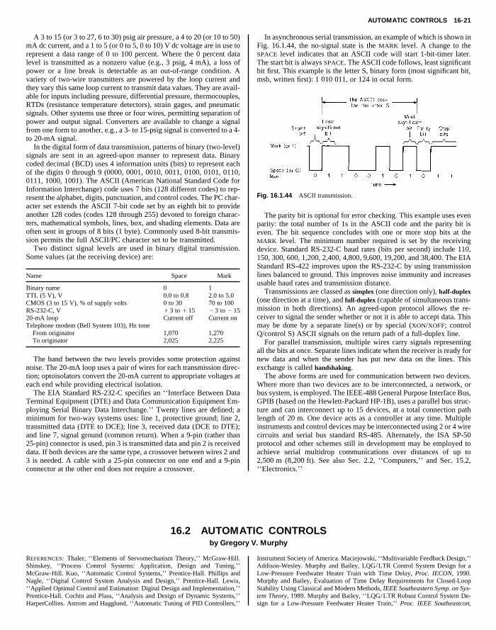
AUTOMATIC CONTROLS 16-21
A 3 to 15 (or 3 to 27, 6 to 30) psig air pressure, a 4 to 20 (or 10 to 50)mA dc current, and a 1 to 5 (or 0 to 5, 0 to 10) V dc voltage are in use torepresent a data range of 0 to 100 percent. Where the 0 percent datalevel is transmitted as a nonzero value (e.g., 3 psig, 4 mA), a loss ofpower or a line break is detectable as an out-of-range condition. Avariety of two-wire transmitters are powered by the loop current andthey vary this same loop current to transmit data values. They are avail-able for inputs including pressure, differential pressure, thermocouples,RTDs (resistance temperature detectors), strain gages, and pneumaticsignals. Other systems use three or four wires, permitting separation of
In asynchronous serial transmission, an example of which is shown inFig. 16.1.44, the no-signal state is the MARK level. A change to theSPACE level indicates that an ASCII code will start 1-bit-timer later.The start bit is always SPACE. The ASCII code follows, least significantbit first. This example is the letter S, binary form (most significant bit,msb, written first): 1 010 011, or 124 in octal form.
TIy V
Copyright (C) 1999 by The McGraw-Hill Companies, Inc. All rights reserved. Use ofthis product is subject to the terms of its License Agreement. Click here to view.
power and output signal. Converters are available to change a signalfrom one form to another, e.g., a 3- to 15-psig signal is converted to a 4-to 20-mA signal.
In the digital form of data transmission, patterns of binary (two-level)signals are sent in an agreed-upon manner to represent data. Binarycoded decimal (BCD) uses 4 information units (bits) to represent eachof the digits 0 through 9 (0000, 0001, 0010, 0011, 0100, 0101, 0110,0111, 1000, 1001). The ASCII (American National Standard Code forInformation Interchange) code uses 7 bits (128 different codes) to rep-resent the alphabet, digits, punctuation, and control codes. The PC char-acter set extends the ASCII 7-bit code set by an eighth bit to provideanother 128 codes (codes 128 through 255) devoted to foreign charac-ters, mathematical symbols, lines, box, and shading elements. Data areoften sent in groups of 8 bits (1 byte). Commonly used 8-bit transmis-sion permits the full ASCII/PC character set to be transmitted.
Two distinct signal levels are used in binary digital transmission.Some values (at the receiving device) are:
Name Space Mark
Binary name 0 1TTL (5 V), V 0.0 to 0.8 2.0 to 5.0CMOS (3 to 15 V), % of supply volts 0 to 30 70 to 100RS-232-C, V 1 3 to 1 15 2 3 to 2 1520-mA loop Current off Current onTelephone modem (Bell System 103), Hz tone
From originator 1,070 1,270To originator 2,025 2,225
The band between the two levels provides some protection againstnoise. The 20-mA loop uses a pair of wires for each transmission direc-tion; optoisolators convert the 20-mA current to appropriate voltages ateach end while providing electrical isolation.
The EIA Standard RS-232-C specifies an ‘‘Interface Between DataTerminal Equipment (DTE) and Data Communication Equipment Em-ploying Serial Binary Data Interchange.’’ Twenty lines are defined; aminimum for two-way systems uses: line 1, protective ground; line 2,transmitted data (DTE to DCE); line 3, received data (DCE to DTE);and line 7, signal ground (common return). When a 9-pin (rather than25-pin) connector is used, pin 3 is transmitted data and pin 2 is receiveddata. If both devices are the same type, a crossover between wires 2 and3 is needed. A cable with a 25-pin connector on one end and a 9-pinconnector at the other end does not require a crossover.
16.2 AUTOMAby Gregor
REFERENCES: Thaler, ‘‘Elements of Servomechanism Theory,’’ McGraw-Hill.
Shinskey, ‘‘Process Control Systems: Application, Design and Tuning,’’McGraw-Hill. Kuo, ‘‘Automatic Control Systems,’’ Prentice-Hall. Phillips andNagle, ‘‘Digital Control System Analysis and Design,’’ Prentice-Hall. Lewis,‘‘Applied Optimal Control and Estimation: Digital Design and Implementation,’’Prentice-Hall. Cochin and Plass, ‘‘Analysis and Design of Dynamic Systems,’’HarperCollins. Astrom and Hagglund, ‘‘Automatic Tuning of PID Controllers,’’Fig. 16.1.44 ASCII transmission.
The parity bit is optional for error checking. This example uses evenparity: the total number of 1s in the ASCII code and the parity bit iseven. The bit sequence concludes with one or more stop bits at theMARK level. The minimum number required is set by the receivingdevice. Standard RS-232-C baud rates (bits per second) include 110,150, 300, 600, 1,200, 2,400, 4,800, 9,600, 19,200, and 38,400. The EIAStandard RS-422 improves upon the RS-232-C by using transmissionlines balanced to ground. This improves noise immunity and increasesusable baud rates and transmission distance.
Transmissions are classed as simplex (one direction only), half-duplex(one direction at a time), and full-duplex (capable of simultaneous trans-mission in both directions). An agreed-upon protocol allows the re-ceiver to signal the sender whether or not it is able to accept data. Thismay be done by a separate line(s) or by special (XON/XOFF; controlQ/control S) ASCII signals on the return path of a full-duplex line.
For parallel transmission, multiple wires carry signals representingall the bits at once. Separate lines indicate when the receiver is ready fornew data and when the sender has put new data on the lines. Thisexchange is called handshaking.
The above forms are used for communication between two devices.Where more than two devices are to be interconnected, a network, orbus system, is employed. The IEEE-488 General Purpose Interface Bus,GPIB (based on the Hewlett-Packard HP-1B), uses a parallel bus struc-ture and can interconnect up to 15 devices, at a total connection pathlength of 20 m. One device acts as a controller at any time. Multipleinstruments and control devices may be interconnected using 2 or 4 wirecircuits and serial bus standard RS-485. Alternately, the ISA SP-50protocol and other schemes still in development may be employed toachieve serial multidrop communications over distances of up to2,500 m (8,200 ft). See also Sec. 2.2, ‘‘Computers,’’ and Sec. 15.2,‘‘Electronics.’’
C CONTROLS. Murphy
Instrument Society of America. Maciejowski, ‘‘Multivariable Feedback Design,’’
Addison-Wesley. Murphy and Bailey, LQG/LTR Control System Design for aLow-Pressure Feedwater Heater Train with Time Delay, Proc. IECON, 1990.Murphy and Bailey, Evaluation of Time Delay Requirements for Closed-LoopStability Using Classical and Modern Methods, IEEE Southeastern Symp. on Sys-tem Theory, 1989. Murphy and Bailey, ‘‘LQG/LTR Robust Control System De-sign for a Low-Pressure Feedwater Heater Train,’’ Proc. IEEE Southeastcon,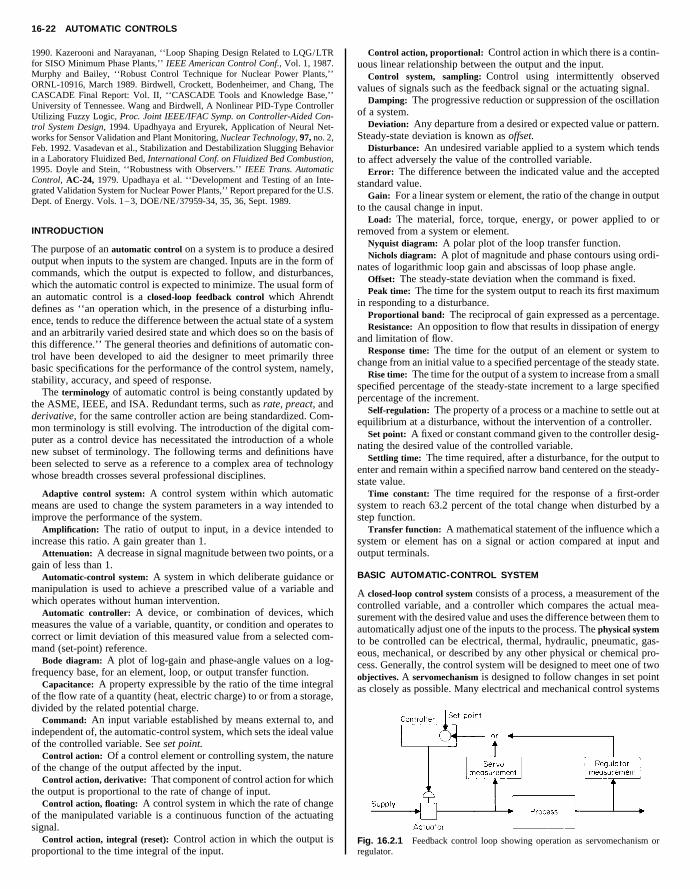
16-22 AUTOMATIC CONTROLS
1990. Kazerooni and Narayanan, ‘‘Loop Shaping Design Related to LQG/LTRfor SISO Minimum Phase Plants,’’ IEEE American Control Conf., Vol. 1, 1987.Murphy and Bailey, ‘‘Robust Control Technique for Nuclear Power Plants,’’ORNL-10916, March 1989. Birdwell, Crockett, Bodenheimer, and Chang, TheCASCADE Final Report: Vol. II, ‘‘CASCADE Tools and Knowledge Base,’’University of Tennessee. Wang and Birdwell, A Nonlinear PID-Type ControllerUtilizing Fuzzy Logic, Proc. Joint IEEE/IFAC Symp. on Controller-Aided Con-trol System Design, 1994. Upadhyaya and Eryurek, Application of Neural Net-works for Sensor Validation and Plant Monitoring, Nuclear Technology, 97, no. 2,Feb. 1992. Vasadevan et al., Stabilization and Destabilization Slugging Behaviorin a Laboratory Fluidized Bed, International Conf. on Fluidized Bed Combustion,
Control action, proportional: Control action in which there is a contin-uous linear relationship between the output and the input.
Control system, sampling: Control using intermittently observedvalues of signals such as the feedback signal or the actuating signal.
Damping: The progressive reduction or suppression of the oscillationof a system.
Deviation: Any departure from a desired or expected value or pattern.Steady-state deviation is known as offset.
Disturbance: An undesired variable applied to a system which tendsto affect adversely the value of the controlled variable.
Copyright (C) 1999 by The McGraw-Hill Companies, Inc. All rights reserved. Use ofthis product is subject to the terms of its License Agreement. Click here to view.
1995. Doyle and Stein, ‘‘Robustness with Observers.’’ IEEE Trans. AutomaticControl, AC-24, 1979. Upadhaya et al. ‘‘Development and Testing of an Inte-grated Validation System for Nuclear Power Plants,’’ Report prepared for the U.S.Dept. of Energy. Vols. 1–3, DOE/NE/37959-34, 35, 36, Sept. 1989.
INTRODUCTION
The purpose of an automatic control on a system is to produce a desiredoutput when inputs to the system are changed. Inputs are in the form ofcommands, which the output is expected to follow, and disturbances,which the automatic control is expected to minimize. The usual form ofan automatic control is a closed-loop feedback control which Ahrendtdefines as ‘‘an operation which, in the presence of a disturbing influ-ence, tends to reduce the difference between the actual state of a systemand an arbitrarily varied desired state and which does so on the basis ofthis difference.’’ The general theories and definitions of automatic con-trol have been developed to aid the designer to meet primarily threebasic specifications for the performance of the control system, namely,stability, accuracy, and speed of response.
The terminology of automatic control is being constantly updated bythe ASME, IEEE, and ISA. Redundant terms, such as rate, preact, andderivative, for the same controller action are being standardized. Com-mon terminology is still evolving. The introduction of the digital com-puter as a control device has necessitated the introduction of a wholenew subset of terminology. The following terms and definitions havebeen selected to serve as a reference to a complex area of technologywhose breadth crosses several professional disciplines.
Adaptive control system: A control system within which automaticmeans are used to change the system parameters in a way intended toimprove the performance of the system.
Amplification: The ratio of output to input, in a device intended toincrease this ratio. A gain greater than 1.
Attenuation: A decrease in signal magnitude between two points, or again of less than 1.
Automatic-control system: A system in which deliberate guidance ormanipulation is used to achieve a prescribed value of a variable andwhich operates without human intervention.
Automatic controller: A device, or combination of devices, whichmeasures the value of a variable, quantity, or condition and operates tocorrect or limit deviation of this measured value from a selected com-mand (set-point) reference.
Bode diagram: A plot of log-gain and phase-angle values on a log-frequency base, for an element, loop, or output transfer function.
Capacitance: A property expressible by the ratio of the time integralof the flow rate of a quantity (heat, electric charge) to or from a storage,divided by the related potential charge.
Command: An input variable established by means external to, andindependent of, the automatic-control system, which sets the ideal valueof the controlled variable. See set point.
Control action: Of a control element or controlling system, the natureof the change of the output affected by the input.
Control action, derivative: That component of control action for whichthe output is proportional to the rate of change of input.
Control action, floating: A control system in which the rate of changeof the manipulated variable is a continuous function of the actuatingsignal.
Control action, integral (reset): Control action in which the output isproportional to the time integral of the input.
Error: The difference between the indicated value and the acceptedstandard value.
Gain: For a linear system or element, the ratio of the change in outputto the causal change in input.
Load: The material, force, torque, energy, or power applied to orremoved from a system or element.
Nyquist diagram: A polar plot of the loop transfer function.Nichols diagram: A plot of magnitude and phase contours using ordi-
nates of logarithmic loop gain and abscissas of loop phase angle.Offset: The steady-state deviation when the command is fixed.Peak time: The time for the system output to reach its first maximum
in responding to a disturbance.Proportional band: The reciprocal of gain expressed as a percentage.Resistance: An opposition to flow that results in dissipation of energy
and limitation of flow.Response time: The time for the output of an element or system to
change from an initial value to a specified percentage of the steady state.Rise time: The time for the output of a system to increase from a small
specified percentage of the steady-state increment to a large specifiedpercentage of the increment.
Self-regulation: The property of a process or a machine to settle out atequilibrium at a disturbance, without the intervention of a controller.
Set point: A fixed or constant command given to the controller desig-nating the desired value of the controlled variable.
Settling time: The time required, after a disturbance, for the output toenter and remain within a specified narrow band centered on the steady-state value.
Time constant: The time required for the response of a first-ordersystem to reach 63.2 percent of the total change when disturbed by astep function.
Transfer function: A mathematical statement of the influence which asystem or element has on a signal or action compared at input andoutput terminals.
BASIC AUTOMATIC-CONTROL SYSTEM
A closed-loop control system consists of a process, a measurement of thecontrolled variable, and a controller which compares the actual mea-surement with the desired value and uses the difference between them toautomatically adjust one of the inputs to the process. The physical systemto be controlled can be electrical, thermal, hydraulic, pneumatic, gas-eous, mechanical, or described by any other physical or chemical pro-cess. Generally, the control system will be designed to meet one of twoobjectives. A servomechanism is designed to follow changes in set pointas closely as possible. Many electrical and mechanical control systems
Fig. 16.2.1 Feedback control loop showing operation as servomechanism orregulator.
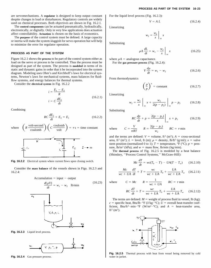
PROCESS AS PART OF THE SYSTEM 16-23
are servomechanisms. A regulator is designed to keep output constantdespite changes in load or disturbances. Regulatory controls are widelyused on chemical processes. Both objectives are shown in Fig. 16.2.1.
The control components can be actuated pneumatically, hydraulically,electronically, or digitally. Only in very few applications does actuationaffect controllability. Actuation is chosen on the basis of economics.
The purpose of the control system must be defined. A large capacityor inertia will make the system sluggish for servo operation but will helpto minimize the error for regulator operation.
For the liquid level process (Fig. 16.2.3):
V 5 A L (16.2.4)
Linearizing
w2 5w2
xU
ss
x
Substituting
dL w2
Copyright (C) 1999 by The McGraw-Hill Companies, Inc. All rights reserved. Use ofthis product is subject to the terms of its License Agreement. Click here to view.
PROCESS AS PART OF THE SYSTEM
Figure 16.2.1 shows the process to be part of the control system either asload on the servo or process to be controlled. Thus the process must bedesigned as part of the system. The process is modeled in terms of itsstatic and dynamic gains in order that it be incorporated into the systemdiagram. Modeling uses Ohm’s and Kirchhoff’s laws for electrical sys-tems, Newton’s laws for mechanical systems, mass balances for fluid-flow systems, and energy balances for thermal systems.
Consider the electrical system in Fig. 16.2.2
i 5E1 2 E2
R
i 5 CdE2
dt
(16.2.1)
Combining
RCdE2
dt1 E2 5 E1 (16.2.2)
where SRvolt-second
coulomb DSCcoulomb
volt D 5 t s 5 time constant
Fig. 16.2.2 Electrical system where current flows upon closing switch.
Consider the mass balance of the vessels shown in Figs. 16.2.3 and16.2.4:
Accumulation 5 input 2 output
d(rV)
dt5 w1 2 w2 lb/min
(16.23)
Fig. 16.2.3 Liquid level process.
Fig. 16.2.4 Gas pressure process.
rAdt
5 w1 2xU
ss
x (16.25)
where rA 5 analogous capacitance.For the gas pressure process (Fig. 16.2.4):
Vdr
dt5 w1 2 w2 (16.2.6)
From thermodynamics
Sr
pDn
5 constant (16.2.7)
Linearizing
w2 5w2
x Uss
x 1w2
2(p 2 p2) Uss
p 2 p2 (16.2.8)
Substituting
RCdp
dt1 p 5
2(p 2 p2)
x Uss
x 1 p2 (16.2.9)
where C 5V
nRTR 5
2(p 2 p2)
w2
RC 5 t min
and the terms are defined: V 5 volume, ft3 (m3); A 5 cross-sectionalarea, ft2 (m2); L 5 level, ft (m); r 5 density, lb/ft3 (g/ml); x 5 valvestem position (normalized 0 to 1); T 5 temperature, °F (°C); p 5 pres-sure, lb/in2 (kPa); and w 5 mass flow, lb/min (kg/min).
The thermal process of Fig. 16.2.5 is modeled by a heat balance(Shinskey, ‘‘Process Control Systems,’’ McGraw-Hill):
McdT
dt5 wc(T0 2 T ) 2 UA(T 2 Tw) (16.2.10)
Mc
wc 1 UA
dT
dt1 T 5
wc
wc 1 UAT0 1
UA
wc 1 UATw (16.2.11)
where C 5 Mc R 51
wc 1 UARC 5 t min
RCdT
dt1 T 5
wc
wc 1 UAT0 1
UA
wc 1 UATw (16.2.12)
The terms are defined: M 5 weight of process fluid in vessel, lb (kg);c 5 specific heat, Btu/lb ?°F (J/kg ?°C); U 5 overall heat-transfer coef-ficient, Btu/ft2 ?min ?°F (W/m2 ?°C); and A 5 heat-transfer area,ft2 (m2).
Fig. 16.2.5 Thermal process with heat from vessel being removed by coldwater in jacket.
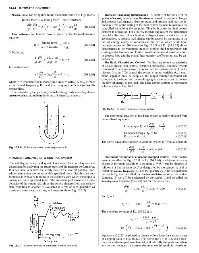
16-24 AUTOMATIC CONTROLS
Newton’s laws can be applied to the manometer shown in Fig. 16.2.6.
Inertia force 5 restoring force 2 flow resistance
Alr
gc
d2h
dt25 ASp 2 2hr
g
gcD 2 RA
dh
dt(16.2.13)
Flow resistance for laminar flow is given by the Hagen-Poiseuilleequation:
R 5driving force
5321m
2(16.2.14)
Transient-Producing Disturbances A number of factors affect thequality of control, among them disturbances caused by set-point changesand process-load changes. Both set point and process load may be de-fined in terms of the setting of the final control element to maintain thecontrolled variable at the set point. Thus both cause the final controlelement to reposition. For a purely mechanical system the disturbancemay take the form of a vibration, a displacement, a velocity, or anacceleration. A process-load change can be caused by variations in therate of energy supply or variations in the rate at which work flowsthrough the process. Reference to Fig. 16.2.5 and Eq. (16.2.12) shows
rate of transfer d gcSubstituting
1
2g
d2h
dt21
161m
rdg2
dh
dt1 h 5 hi (16.2.15)
In standard form
t 2c
d2h
dt21 2tcz
dh
dt1 h 5 hi (16.2.16)
where tc 5 characteristic response time, min, 5 1/[(60) (2p)vn] wherevn 5 natural frequency, Hz; and z 5 damping coefficient (ratio), di-mensionless.
The variables tc and z are very valuable design aids since they definesystem response and stability in terms of system parameters.
Fig. 16.2.6 Filled manometer measuring pressure P.
TRANSIENT ANALYSIS OF A CONTROL SYSTEM
The stability, accuracy, and speed of response of a control system aredetermined by analyzing the steady-state and the transient performance.It is desirable to achieve the steady state in the shortest possible time,while maintaining the output within specified limits. Steady-state per-formance is evaluated in terms of the accuracy with which the output iscontrolled for a specified input. The transient performance, i.e., thebehavior of the output variable as the system changes from one steady-state condition to another, is evaluated in terms of such quantities asmaximum overshoot, rise time, and response time (Fig. 16.2.7).
Fig. 16.2.7 System response to a unit step-function command.
disturbances to be variations in inlet process fluid temperature andcooling-water temperature. Further linearization would show variationsin process flow and the overall heat-transfer coefficient to also be dis-turbances.
The Basic Closed-Loop Control To illustrate some characteristicsof a basic closed-loop control, consider a mechanical, rotational systemcomposed of a prime mover or motor, a total system inertia J, and aviscous friction f. To control the system’s output variable uo , a com-mand signal ui must be supplied, the output variable measured andcompared to the input, and the resulting signal difference used to controlthe flow of energy to the load. The basic control system is representedschematically in Fig. 16.2.8.
Fig. 16.2.8 A basic closed-loop control system.
The differential equation of this basic system is readily obtained fromthe idealized equations
Load torque TL 5 Jd2uo
dt21 f
duo
dt(16.2.17)
Developed torque TD 5 K« (16.2.18)Error « 5 ui 2 uo (16.2.19)
The above equations combine to yield the system differential equation:
Jd2uo
dt21 f
duo
dt1 Kuo 5 Kui (16.2.20)
Step-Input Response of a Viscous-Damped Control If the controlsystem described in Fig. 16.2.8 by Eq. (16.2.20) is subjected to a stepchange in the input variable ui , a solution uo 5 uo(t) can be obtained asfollows. (1) Let the ratio √K/J be designated by the symbol vn and becalled the natural frequency. (2) Let the quantity 2√JK be designated bythe symbol fc and be called the friction coefficient required for criticaldamping. (3) Let f /fc be designated by the symbol z and be called thedamping ratio. Equation (16.2.20) can then be written as
d2uo
dt21 2zvn
duo
dt1 v2
nuo 5 v2nui (16.2.21)
For ui 5 1:
uo 5 0 andduo
dt5 0 at t 5 0
The complete solution of Eq. (16.2.21) is
uo 5 1 2exp (2zvnt)
√1 2 z 2
sin S√1 2 z 2vnt 1 tan21√1 2 z 2
zD (16.2.22)
Equation (16.2.22) is plotted in dimensionless form for various valuesof damping ratio in Fig. 16.2.9. The curves for z 5 0.1, 2, and 1 illus-trate the underdamped, overdamped, and critically damped case, whereany further decrease in system damping would result in overshoot.
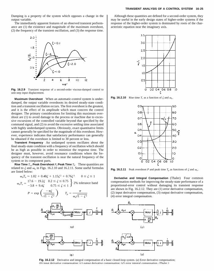
TRANSIENT ANALYSIS OF A CONTROL SYSTEM 16-25
Damping is a property of the system which opposes a change in theoutput variable.
The immediately apparent features of an observed transient perform-ance are (1) the existence and magnitude of the maximum overshoot,(2) the frequency of the transient oscillation, and (3) the response time.
Although these quantities are defined for a second-order system, theymay be useful in the early design states of higher-order systems if theresponse of the higher-order system is dominated by roots of the char-acteristic equation near the imaginary axis.
Copyright (C) 1999 by The McGraw-Hill Companies, Inc. All rights reserved. Use ofthis product is subject to the terms of its License Agreement. Click here to view.
Fig. 16.2.9 Transient response of a second-order viscous-damped control tounit-step input displacement.
Maximum Overshoot When an automatic-control system is under-damped, the output variable overshoots its desired steady-state condi-tion and a transient oscillation occurs. The first overshoot is the greatest,and it is the effect of its amplitude which must concern the controldesigner. The primary considerations for limiting this maximum over-shoot are (1) to avoid damage to the process or machine due to exces-sive excursions of the controlled variable beyond that specified by thecommand signal, and (2) to avoid the excessive settling time associatedwith highly underdamped systems. Obviously, exact quantitative limitscannot generally be specified for the magnitude of this overshoot. How-ever, experience indicates that satisfactory performance can generallybe obtained if the overshoot is limited to 30 percent or less.
Transient Frequency An undamped system oscillates about thefinal steady-state condition with a frequency of oscillation which shouldbe as high as possible in order to minimize the response time. Thedesigner must, however, avoid resonance conditions where the fre-quency of the transient oscillation is near the natural frequency of thesystem or its component parts.
Rise Time Tn , Peak Overshoot P, Peak Time TP These quantities arerelated to z and vn in Figs. 16.2.10 and 16.2.11. Some useful formulasare listed below:
vnTn ' 1.02 1 0.48z 1 1.15z 2 1 0.76z 3 0 # z # 1
vnTs 517.6 2 19.2z 0.2 # z # 0.75
23.8 1 9.4z 0.75 # z # 1J 2% tolerance band
P 5 expS 2pz
√1 2 z 2D Tp 5
p
vn√1 2 z 2
Fig. 16.2.12 Derivative and integral compensation of a bas(b) input derivative compensation; (c) output derivative comp
Fig. 16.2.10 Rise time Tr as a function of z and vn .
Fig. 16.2.11 Peak overshoot P and peak time Tp as functions of z and vn .
Derivative and Integral Compensation (Thaler) Four commoncompensation methods for improving the steady-state performance of aproportional-error control without damaging its transient responseare shown in Fig. 16.2.12. They are (1) error derivative compensation,(2) input derivative compensation, (3) output derivative compensation,(4) error integral compensation.
ic closed-loop system. (a) Error derivative compensation;ensation; (d ) error integral compensation. (Thaler.)
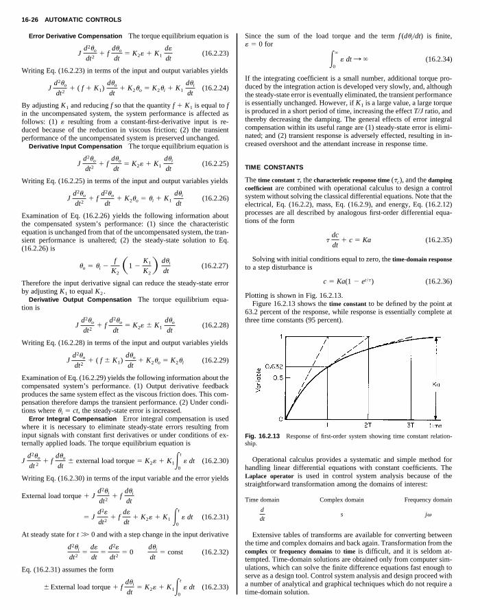
16-26 AUTOMATIC CONTROLS
Error Derivative Compensation The torque equilibrium equation is
Jd2uo
dt21 f
duo
dt5 K2« 1 K1
d«
dt(16.2.23)
Writing Eq. (16.2.23) in terms of the input and output variables yields
Jd2uo
dt21 ( f 1 K1)
duo
dt1 K2uo 5 K2ui 1 K1
dui
dt(16.2.24)
By adjusting K1 and reducing f so that the quantity f 1 K1 is equal to f
Since the sum of the load torque and the term f (dui/dt) is finite,« 5 0 for
E`
0
« dt : ` (16.2.34)
If the integrating coefficient is a small number, additional torque pro-duced by the integration action is developed very slowly, and, althoughthe steady-state error is eventually eliminated, the transient performanceis essentially unchanged. However, if K1 is a large value, a large torqueis produced in a short period of time, increasing the effect T/J ratio, and
in the uncompensated system, the system performance is affected asfollows: (1) « resulting from a constant-first-derivative input is re-duced because of the reduction in viscous friction; (2) the transientperformance of the uncompensated system is preserved unchanged.
Derivative Input Compensation The torque equilibrium equation is
Jd2uo
dt21 f
duo
dt5 K2« 1 K1
dui
dt(16.2.25)
Writing Eq. (16.2.25) in terms of the input and output variables yields
Jd2uo
dt21 f
d2uo
dt1 K2uo 5 ui 1 K1
dui
dt(16.2.26)
Examination of Eq. (16.2.26) yields the following information aboutthe compensated system’s performance: (1) since the characteristicequation is unchanged from that of the uncompensated system, the tran-sient performance is unaltered; (2) the steady-state solution to Eq.(16.2.26) is
uo 5 ui 2f
K2S1 2
K1
K2D dui
dt(16.2.27)
Therefore the input derivative signal can reduce the steady-state errorby adjusting K1 to equal K2 .
Derivative Output Compensation The torque equilibrium equa-tion is
Jd2uo
dt21 f
d2uo
dt5 K2« 6 K1
duo
dt(16.2.28)
Writing Eq. (16.2.28) in terms of the input and output variables yields
Jd2uo
dt21 ( f 6 K1)
duo
dt1 K2uo 5 K2ui (16.2.29)
Examination of Eq. (16.2.29) yields the following information about thecompensated system’s performance. (1) Output derivative feedbackproduces the same system effect as the viscous friction does. This com-pensation therefore damps the transient performance. (2) Under condi-tions where ui 5 ct, the steady-state error is increased.
Error Integral Compensation Error integral compensation is usedwhere it is necessary to eliminate steady-state errors resulting frominput signals with constant first derivatives or under conditions of ex-ternally applied loads. The torque equilibrium equation is
Jd2uo
dt 21 f
duo
dt6 external load torque 5 K2« 1 K1Et
0
« dt (16.2.30)
Writing Eq. (16.2.30) in terms of the input variable and the error yields
External load torque 1 Jd2ui
dt21 f
dui
dt
5 Jd2«
dt21 f
d«
dt1 K2« 1 K1 Et
0
« dt (16.2.31)
At steady state for t .. 0 and with a step change in the input derivative
d2ui
dt25
d«
dt5
d2«
dt25 0
dui
dt5 const (16.2.32)
Eq. (16.2.31) assumes the form
6 External load torque 1 fdui
dt5 K2« 1 K1Et
0
« dt (16.2.33)
thereby decreasing the damping. The general effects of error integralcompensation within its useful range are (1) steady-state error is elimi-nated; and (2) transient response is adversely effected, resulting in in-creased overshoot and the attendant increase in response time.
TIME CONSTANTS
The time constant t, the characteristic response time (tc), and the dampingcoefficient are combined with operational calculus to design a controlsystem without solving the classical differential equations. Note that theelectrical, Eq. (16.2.2), mass, Eq. (16.2.9), and energy, Eq. (16.2.12)processes are all described by analogous first-order differential equa-tions of the form
tdc
dt1 c 5 Ka (16.2.35)
Solving with initial conditions equal to zero, the time-domain responseto a step disturbance is
c 5 Ka(1 2 et /t ) (16.2.36)
Plotting is shown in Fig. 16.2.13.Figure 16.2.13 shows the time constant to be defined by the point at
63.2 percent of the response, while response is essentially complete atthree time constants (95 percent).
Fig. 16.2.13 Response of first-order system showing time constant relation-ship.
Operational calculus provides a systematic and simple method forhandling linear differential equations with constant coefficients. TheLaplace operator is used in control system analysis because of thestraightforward transformation among the domains of interest:
Time domain Complex domain Frequency domain
d
dts jv
Extensive tables of transforms are available for converting betweenthe time and complex domains and back again. Transformation from thecomplex or frequency domains to time is difficult, and it is seldom at-tempted. Time-domain solutions are obtained only from computer sim-ulations, which can solve the finite difference equations fast enough toserve as a design tool. Control system analysis and design proceed witha number of analytical and graphical techniques which do not require atime-domain solution.
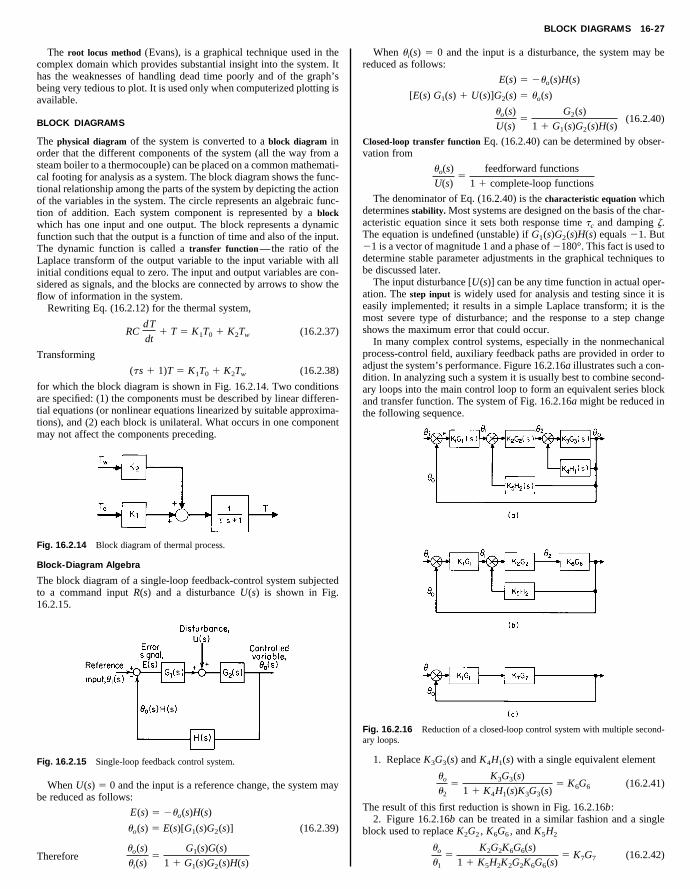
BLOCK DIAGRAMS 16-27
The root locus method (Evans), is a graphical technique used in thecomplex domain which provides substantial insight into the system. Ithas the weaknesses of handling dead time poorly and of the graph’sbeing very tedious to plot. It is used only when computerized plotting isavailable.
BLOCK DIAGRAMS
The physical diagram of the system is converted to a block diagram inorder that the different components of the system (all the way from a
When ui(s) 5 0 and the input is a disturbance, the system may bereduced as follows:
E(s) 5 2uo(s)H(s)
[E(s) G1(s) 1 U(s)]G2(s) 5 uo(s)
uo(s)
U(s)5
G2(s)
1 1 G1(s)G2(s)H(s)(16.2.40)
Closed-loop transfer function Eq. (16.2.40) can be determined by obser-vation from
steam boiler to a thermocouple) can be placed on a common mathemati-cal footing for analysis as a system. The block diagram shows the func-tional relationship among the parts of the system by depicting the actionof the variables in the system. The circle represents an algebraic func-tion of addition. Each system component is represented by a blockwhich has one input and one output. The block represents a dynamicfunction such that the output is a function of time and also of the input.The dynamic function is called a transfer function—the ratio of theLaplace transform of the output variable to the input variable with allinitial conditions equal to zero. The input and output variables are con-sidered as signals, and the blocks are connected by arrows to show theflow of information in the system.
Rewriting Eq. (16.2.12) for the thermal system,
RCdT
dt1 T 5 K1T0 1 K2Tw (16.2.37)
Transforming
(ts 1 1)T 5 K1T0 1 K2Tw (16.2.38)
for which the block diagram is shown in Fig. 16.2.14. Two conditionsare specified: (1) the components must be described by linear differen-tial equations (or nonlinear equations linearized by suitable approxima-tions), and (2) each block is unilateral. What occurs in one componentmay not affect the components preceding.
Fig. 16.2.14 Block diagram of thermal process.
Block-Diagram Algebra
The block diagram of a single-loop feedback-control system subjectedto a command input R(s) and a disturbance U(s) is shown in Fig.16.2.15.
Fig. 16.2.15 Single-loop feedback control system.
When U(s) 5 0 and the input is a reference change, the system maybe reduced as follows:
E(s) 5 2uo(s)H(s)
uo(s) 5 E(s)[G1(s)G2(s)] (16.2.39)
uo(s)
ui(s)5
G1(s)G(s)
1 1 G1(s)G2(s)H(s)Therefore
uo(s)
U(s)5
feedforward functions
1 1 complete-loop functions
The denominator of Eq. (16.2.40) is the characteristic equation whichdetermines stability. Most systems are designed on the basis of the char-acteristic equation since it sets both response time tc and damping z.The equation is undefined (unstable) if G1(s)G2(s)H(s) equals 21. But21 is a vector of magnitude 1 and a phase of 2180°. This fact is used todetermine stable parameter adjustments in the graphical techniques tobe discussed later.
The input disturbance [U(s)] can be any time function in actual oper-ation. The step input is widely used for analysis and testing since it iseasily implemented; it results in a simple Laplace transform; it is themost severe type of disturbance; and the response to a step changeshows the maximum error that could occur.
In many complex control systems, especially in the nonmechanicalprocess-control field, auxiliary feedback paths are provided in order toadjust the system’s performance. Figure 16.2.16a illustrates such a con-dition. In analyzing such a system it is usually best to combine second-ary loops into the main control loop to form an equivalent series blockand transfer function. The system of Fig. 16.2.16a might be reduced inthe following sequence.
Fig. 16.2.16 Reduction of a closed-loop control system with multiple second-ary loops.
1. Replace K3G3(s) and K4H1(s) with a single equivalent element
uo
u2
5K3G3(s)
1 1 K4H1(s)K3G3(s)5 K6G6 (16.2.41)
The result of this first reduction is shown in Fig. 16.2.16b:2. Figure 16.2.16b can be treated in a similar fashion and a single
block used to replace K2G2 , K6G6 , and K5H2
uo
u1
5K2G2K6G6(s)
1 1 K5H2K2G2K6G6(s)5 K7G7 (16.2.42)
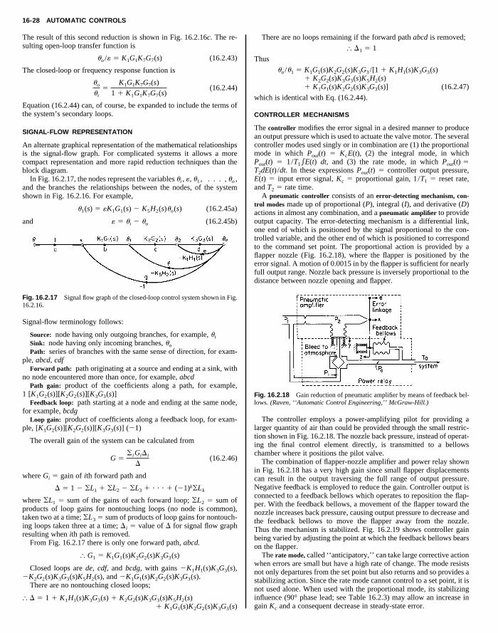
16-28 AUTOMATIC CONTROLS
The result of this second reduction is shown in Fig. 16.2.16c. The re-sulting open-loop transfer function is
uo /« 5 K1G1K7G7(s) (16.2.43)
The closed-loop or frequency response function is
uo
ui
5K1G1K7G7(s)
1 1 K1G1K7G7(s)(16.2.44)
Equation (16.2.44) can, of course, be expanded to include the terms ofthe system’s secondary loops.
There are no loops remaining if the forward path abcd is removed;
[ D1 5 1
Thus
uo /u1 5 K1G1(s)K2G2(s)K3G3 /[1 1 K1H1(s)K3G3(s)1 K2G2(s)K3G3(s)K5H2(s)1 K1G1(s)K2G2(s)K3G3(s)] (16.2.47)
which is identical with Eq. (16.2.44).
CONTROLLER MECHANISMS
Copyright (C) 1999 by The McGraw-Hill Companies, Inc. All rights reserved. Use ofthis product is subject to the terms of its License Agreement. Click here to view.
SIGNAL-FLOW REPRESENTATION
An alternate graphical representation of the mathematical relationshipsis the signal-flow graph. For complicated systems it allows a morecompact representation and more rapid reduction techniques than theblock diagram.
In Fig. 16.2.17, the nodes represent the variables ui , «, u1 , . . . , uo ,and the branches the relationships between the nodes, of the systemshown in Fig. 16.2.16. For example,
u1(s) 5 «K1G1(s) 2 K5H2(s)uo(s) (16.2.45a)
and « 5 ui 2 uo (16.2.45b)
Fig. 16.2.17 Signal flow graph of the closed-loop control system shown in Fig.16.2.16.
Signal-flow terminology follows:
Source: node having only outgoing branches, for example, ui
Sink: node having only incoming branches, uo
Path: series of branches with the same sense of direction, for exam-ple, abcd, cdf
Forward path: path originating at a source and ending at a sink, withno node encountered more than once, for example, abcd
Path gain: product of the coefficients along a path, for example,1 [K1G2(s)][K2G2(s)][K3G3(s)]
Feedback loop: path starting at a node and ending at the same node,for example, bcdg
Loop gain: product of coefficients along a feedback loop, for exam-ple, [K1G2(s)][K2G2(s)][K3G3(s)] (21)
The overall gain of the system can be calculated from
G 5oiGiDi
D(16.2.46)
where Gi 5 gain of ith forward path and
D 5 1 2 oL1 1 oL2 2 oL3 1 ? ? ? 1 (21)koLk
where oL1 5 sum of the gains of each forward loop; oL2 5 sum ofproducts of loop gains for nontouching loops (no node is common),taken two at a time; oL3 5 sum of products of loop gains for nontouch-ing loops taken three at a time; Di 5 value of D for signal flow graphresulting when ith path is removed.
From Fig. 16.2.17 there is only one forward path, abcd.
[ G1 5 K1G1(s)K2G2(s)K3G3(s)
Closed loops are de, cdf, and bcdg, with gains 2K1H1(s)K3G3(s),2K2G2(s)K3G3(s)K5H2(s), and 2K1G1(s)K2G2(s)K3G3(s).
There are no nontouching closed loops;
[ D 5 1 1 K1H1(s)K3G3(s) 1 K2G2(s)K3G3(s)K5H2(s)1 K1G1(s)K2G2(s)K3G3(s)
The controller modifies the error signal in a desired manner to producean output pressure which is used to actuate the valve motor. The severalcontroller modes used singly or in combination are (1) the proportionalmode in which Pout(t) 5 KcE(t), (2) the integral mode, in whichPout(t) 5 1/T1eE(t) dt, and (3) the rate mode, in which Pout(t) 5T2dE(t) /dt. In these expressions Pout(t) 5 controller output pressure,E(t) 5 input error signal, Kc 5 proportional gain, 1/T1 5 reset rate,and T2 5 rate time.
A pneumatic controller consists of an error-detecting mechanism, con-trol modes made up of proportional (P), integral (I), and derivative (D)actions in almost any combination, and a pneumatic amplifier to provideoutput capacity. The error-detecting mechanism is a differential link,one end of which is positioned by the signal proportional to the con-trolled variable, and the other end of which is positioned to correspondto the command set point. The proportional action is provided by aflapper nozzle (Fig. 16.2.18), where the flapper is positioned by theerror signal. A motion of 0.0015 in by the flapper is sufficient for nearlyfull output range. Nozzle back pressure is inversely proportional to thedistance between nozzle opening and flapper.
Fig. 16.2.18 Gain reduction of pneumatic amplifier by means of feedback bel-lows. (Raven, ‘‘Automatic Control Engineering,’’ McGraw-Hill.)
The controller employs a power-amplifying pilot for providing alarger quantity of air than could be provided through the small restric-tion shown in Fig. 16.2.18. The nozzle back pressure, instead of operat-ing the final control element directly, is transmitted to a bellowschamber where it positions the pilot valve.
The combination of flapper-nozzle amplifier and power relay shownin Fig. 16.2.18 has a very high gain since small flapper displacementscan result in the output traversing the full range of output pressure.Negative feedback is employed to reduce the gain. Controller output isconnected to a feedback bellows which operates to reposition the flap-per. With the feedback bellows, a movement of the flapper toward thenozzle increases back pressure, causing output pressure to decrease andthe feedback bellows to move the flapper away from the nozzle.Thus the mechanism is stabilized. Fig. 16.2.19 shows controller gainbeing varied by adjusting the point at which the feedback bellows bearson the flapper.
The rate mode, called ‘‘anticipatory,’’ can take large corrective actionwhen errors are small but have a high rate of change. The mode resistsnot only departures from the set point but also returns and so provides astabilizing action. Since the rate mode cannot control to a set point, it isnot used alone. When used with the proportional mode, its stabilizinginfluence (90° phase lead; see Table 16.2.3) may allow an increase ingain Kc and a consequent decrease in steady-state error.
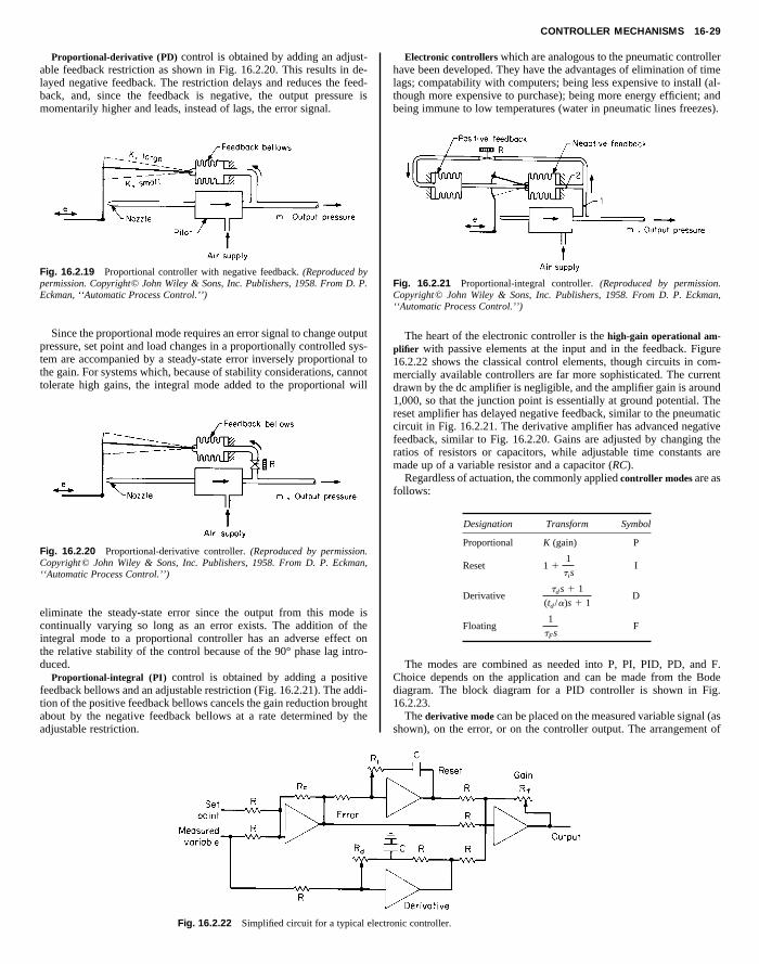
CONTROLLER MECHANISMS 16-29
Proportional-derivative (PD) control is obtained by adding an adjust-able feedback restriction as shown in Fig. 16.2.20. This results in de-layed negative feedback. The restriction delays and reduces the feed-back, and, since the feedback is negative, the output pressure ismomentarily higher and leads, instead of lags, the error signal.
Electronic controllers which are analogous to the pneumatic controllerhave been developed. They have the advantages of elimination of timelags; compatability with computers; being less expensive to install (al-though more expensive to purchase); being more energy efficient; andbeing immune to low temperatures (water in pneumatic lines freezes).
Copyright (C) 1999 by The McGraw-Hill Companies, Inc. All rights reserved. Use ofthis product is subject to the terms of its License Agreement. Click here to view.
Fig. 16.2.19 Proportional controller with negative feedback. (Reproduced bypermission. Copyright© John Wiley & Sons, Inc. Publishers, 1958. From D. P.Eckman, ‘‘Automatic Process Control.’’)
Since the proportional mode requires an error signal to change outputpressure, set point and load changes in a proportionally controlled sys-tem are accompanied by a steady-state error inversely proportional tothe gain. For systems which, because of stability considerations, cannottolerate high gains, the integral mode added to the proportional will
Fig. 16.2.20 Proportional-derivative controller. (Reproduced by permission.Copyright© John Wiley & Sons, Inc. Publishers, 1958. From D. P. Eckman,‘‘Automatic Process Control.’’)
eliminate the steady-state error since the output from this mode iscontinually varying so long as an error exists. The addition of theintegral mode to a proportional controller has an adverse effect onthe relative stability of the control because of the 90° phase lag intro-duced.
Proportional-integral (PI) control is obtained by adding a positivefeedback bellows and an adjustable restriction (Fig. 16.2.21). The addi-tion of the positive feedback bellows cancels the gain reduction broughtabout by the negative feedback bellows at a rate determined by theadjustable restriction.
Fig. 16.2.22 Simplified circuit for a typical electr
Fig. 16.2.21 Proportional-integral controller. (Reproduced by permission.Copyright© John Wiley & Sons, Inc. Publishers, 1958. From D. P. Eckman,‘‘Automatic Process Control.’’)
The heart of the electronic controller is the high-gain operational am-plifier with passive elements at the input and in the feedback. Figure16.2.22 shows the classical control elements, though circuits in com-mercially available controllers are far more sophisticated. The currentdrawn by the dc amplifier is negligible, and the amplifier gain is around1,000, so that the junction point is essentially at ground potential. Thereset amplifier has delayed negative feedback, similar to the pneumaticcircuit in Fig. 16.2.21. The derivative amplifier has advanced negativefeedback, similar to Fig. 16.2.20. Gains are adjusted by changing theratios of resistors or capacitors, while adjustable time constants aremade up of a variable resistor and a capacitor (RC).
Regardless of actuation, the commonly applied controller modes are asfollows:
Designation Transform Symbol
Proportional K (gain) P
Reset 1 11
tisI
Derivativetds 1 1
(td /a)s 1 1D
Floating1
tFsF
The modes are combined as needed into P, PI, PID, PD, and F.Choice depends on the application and can be made from the Bodediagram. The block diagram for a PID controller is shown in Fig.16.2.23.
The derivative mode can be placed on the measured variable signal (asshown), on the error, or on the controller output. The arrangement of
onic controller.
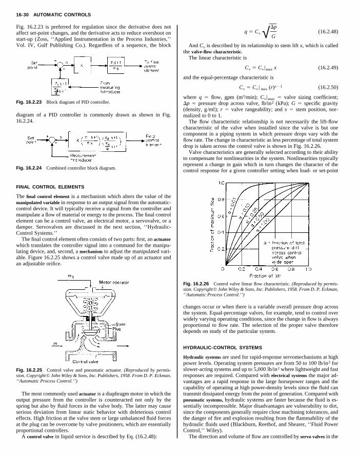
16-30 AUTOMATIC CONTROLS
Fig. 16.2.23 is preferred for regulation since the derivative does notaffect set-point changes, and the derivative acts to reduce overshoot onstart-up (Zoss, ‘‘Applied Instrumentation in the Process Industries,’’Vol. IV, Gulf Publishing Co.). Regardless of a sequence, the block
q 5 Cv √Dp
G(16.2.48)
And Cv is described by its relationship to stem lift x, which is calledthe valve-flow characteristic.
The linear characteristic is
Cv 5 Cv |max x (16.2.49)
and the equal-percentage characteristic is
Copyright (C) 1999 by The McGraw-Hill Companies, Inc. All rights reserved. Use ofthis product is subject to the terms of its License Agreement. Click here to view.
Fig. 16.2.23 Block diagram of PID controller.
diagram of a PID controller is commonly drawn as shown in Fig.16.2.24.
Fig. 16.2.24 Combined controller block diagram.
FINAL CONTROL ELEMENTS
The final control element is a mechanism which alters the value of themanipulated variable in response to an output signal from the automatic-control device. It will typically receive a signal from the controller andmanipulate a flow of material or energy to the process. The final controlelement can be a control valve, an electrical motor, a servovalve, or adamper. Servovalves are discussed in the next section, ‘‘Hydraulic-Control Systems.’’
The final control element often consists of two parts: first, an actuatorwhich translates the controller signal into a command for the manipu-lating device, and, second, a mechanism to adjust the manipulated vari-able. Figure 16.2.25 shows a control valve made up of an actuator andan adjustable orifice.
Fig. 16.2.25 Control valve and pneumatic actuator. (Reproduced by permis-sion. Copyright© John Wiley & Sons, Inc. Publishers, 1958. From D. P. Eckman,‘‘Automatic Process Control.’’)
The most commonly used actuator is a diaphragm motor in which theoutput pressure from the controller is counteracted not only by thespring but also by fluid forces in the valve body. The latter may causeserious deviation from linear static behavior with deleterious controleffects. High friction at the valve stem or large unbalanced fluid forcesat the plug can be overcome by valve positioners, which are essentiallyproportional controllers.
A control valve in liquid service is described by Eq. (16.2.48):
Cv 5 Cv | max (r)x21 (16.2.50)
where q 5 flow, gpm (m3/min); Cv |max 5 valve sizing coefficient;Dp 5 pressure drop across valve, lb/in2 (kPa); G 5 specific gravity(density, g/ml); r 5 valve rangeability; and x 5 stem position, nor-malized to 0 to 1.
The flow characteristic relationship is not necessarily the lift-flowcharacteristic of the valve when installed since the valve is but onecomponent in a piping system in which pressure drops vary with theflow rate. The change in characteristic as less percentage of total systemdrop is taken across the control valve is shown in Fig. 16.2.26.
Valve characteristics are generally selected according to their abilityto compensate for nonlinearities in the system. Nonlinearities typicallyrepresent a change in gain which in turn changes the character of thecontrol response for a given controller setting when load- or set-point
Fig. 16.2.26 Control valve linear flow characteristic. (Reproduced by permis-sion. Copyright© John Wiley & Sons, Inc. Publishers, 1958. From D. P. Eckman,‘‘Automatic Process Control.’’)
changes occur or when there is a variable overall pressure drop acrossthe system. Equal-percentage valves, for example, tend to control overwidely varying operating conditions, since the change in flow is alwaysproportional to flow rate. The selection of the proper valve thereforedepends on study of the particular system.
HYDRAULIC-CONTROL SYSTEMS
Hydraulic systems are used for rapid-response servomechanisms at highpower levels. Operating system pressures are from 50 to 100 lb/in2 forslower-acting systems and up to 5,000 lb/in2 where lightweight and fastresponses are required. Compared with electrical systems the major ad-vantages are a rapid response in the large horsepower ranges and thecapability of operating at high power-density levels since the fluid cantransmit dissipated energy from the point of generation. Compared withpneumatic systems, hydraulic systems are faster because the fluid is es-sentially incompressible. Major disadvantages are vulnerability to dirt,since the components generally require close machining tolerances, andthe danger of fire and explosion resulting from the flammability of thehydraulic fluids used (Blackburn, Reethof, and Shearer, ‘‘Fluid PowerControl,’’ Wiley).
The direction and volume of flow are controlled by servo valves in the
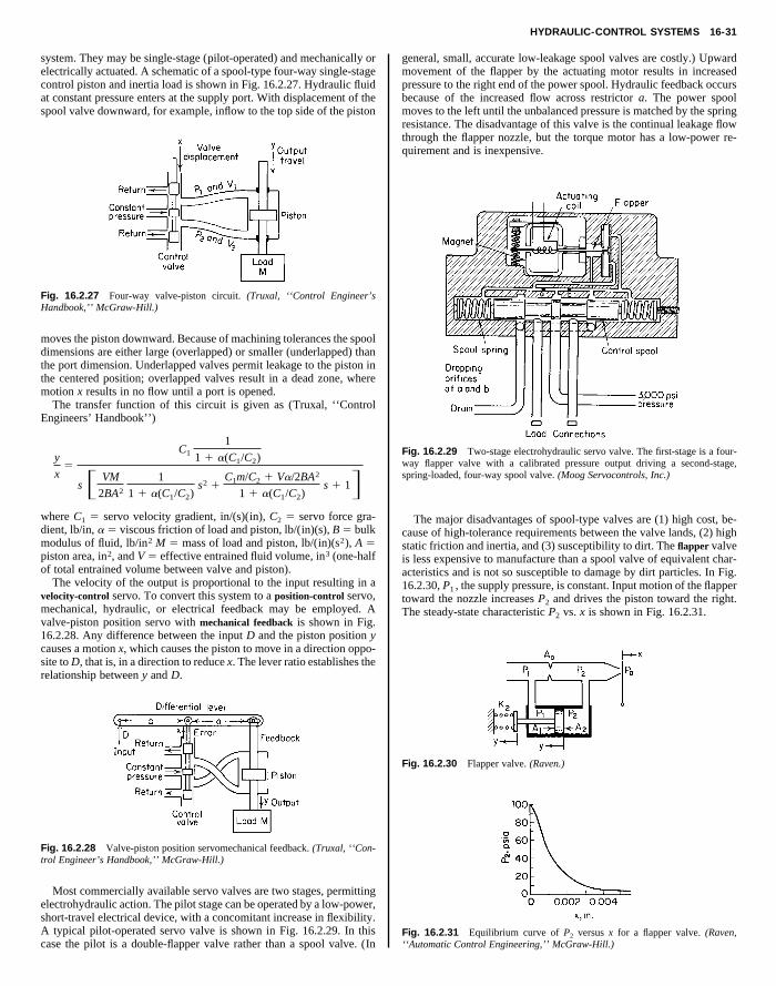
HYDRAULIC-CONTROL SYSTEMS 16-31
system. They may be single-stage (pilot-operated) and mechanically orelectrically actuated. A schematic of a spool-type four-way single-stagecontrol piston and inertia load is shown in Fig. 16.2.27. Hydraulic fluidat constant pressure enters at the supply port. With displacement of thespool valve downward, for example, inflow to the top side of the piston
general, small, accurate low-leakage spool valves are costly.) Upwardmovement of the flapper by the actuating motor results in increasedpressure to the right end of the power spool. Hydraulic feedback occursbecause of the increased flow across restrictor a. The power spoolmoves to the left until the unbalanced pressure is matched by the springresistance. The disadvantage of this valve is the continual leakage flowthrough the flapper nozzle, but the torque motor has a low-power re-quirement and is inexpensive.
Copyright (C) 1999 by The McGraw-Hill Companies, Inc. All rights reserved. Use ofthis product is subject to the terms of its License Agreement. Click here to view.
Fig. 16.2.27 Four-way valve-piston circuit. (Truxal, ‘‘Control Engineer’sHandbook,’’ McGraw-Hill.)
moves the piston downward. Because of machining tolerances the spooldimensions are either large (overlapped) or smaller (underlapped) thanthe port dimension. Underlapped valves permit leakage to the piston inthe centered position; overlapped valves result in a dead zone, wheremotion x results in no flow until a port is opened.
The transfer function of this circuit is given as (Truxal, ‘‘ControlEngineers’ Handbook’’)
y
x5
C1
1
1 1 a(C1/C2)
s F VM
2BA2
1
1 1 a(C1/C2)s2 1
C1m/C2 1 Va/2BA2
1 1 a(C1/C2)s 1 1G
where C1 5 servo velocity gradient, in/(s)(in), C2 5 servo force gra-dient, lb/in, a 5 viscous friction of load and piston, lb/(in)(s), B 5 bulkmodulus of fluid, lb/in2 M 5 mass of load and piston, lb/(in)(s2), A 5piston area, in2, and V 5 effective entrained fluid volume, in3 (one-halfof total entrained volume between valve and piston).
The velocity of the output is proportional to the input resulting in avelocity-control servo. To convert this system to a position-control servo,mechanical, hydraulic, or electrical feedback may be employed. Avalve-piston position servo with mechanical feedback is shown in Fig.16.2.28. Any difference between the input D and the piston position ycauses a motion x, which causes the piston to move in a direction oppo-site to D, that is, in a direction to reduce x. The lever ratio establishes therelationship between y and D.
Fig. 16.2.28 Valve-piston position servomechanical feedback. (Truxal, ‘‘Con-trol Engineer’s Handbook,’’ McGraw-Hill.)
Most commercially available servo valves are two stages, permittingelectrohydraulic action. The pilot stage can be operated by a low-power,short-travel electrical device, with a concomitant increase in flexibility.A typical pilot-operated servo valve is shown in Fig. 16.2.29. In thiscase the pilot is a double-flapper valve rather than a spool valve. (In
Fig. 16.2.29 Two-stage electrohydraulic servo valve. The first-stage is a four-way flapper valve with a calibrated pressure output driving a second-stage,spring-loaded, four-way spool valve. (Moog Servocontrols, Inc.)
The major disadvantages of spool-type valves are (1) high cost, be-cause of high-tolerance requirements between the valve lands, (2) highstatic friction and inertia, and (3) susceptibility to dirt. The flapper valveis less expensive to manufacture than a spool valve of equivalent char-acteristics and is not so susceptible to damage by dirt particles. In Fig.16.2.30, P1 , the supply pressure, is constant. Input motion of the flappertoward the nozzle increases P2 and drives the piston toward the right.The steady-state characteristic P2 vs. x is shown in Fig. 16.2.31.
Fig. 16.2.30 Flapper valve. (Raven.)
Fig. 16.2.31 Equilibrium curve of P2 versus x for a flapper valve. (Raven,‘‘Automatic Control Engineering,’’ McGraw-Hill.)
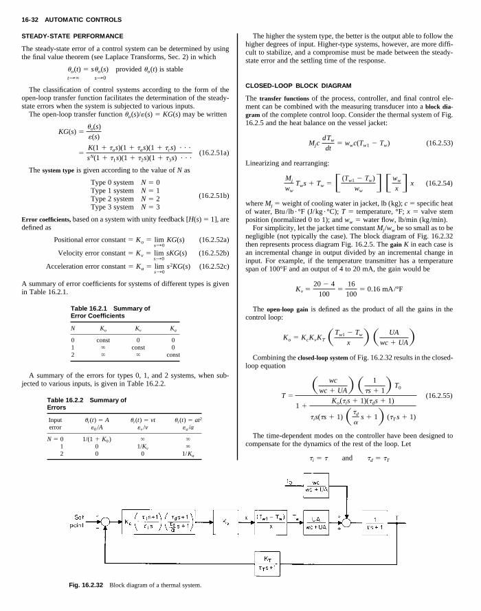
16-32 AUTOMATIC CONTROLS
STEADY-STATE PERFORMANCE
The steady-state error of a control system can be determined by usingthe final value theorem (see Laplace Transforms, Sec. 2) in which
uo(t) 5 suo(s) provided uo(t) is stablet:` s:0
The classification of control systems according to the form of theopen-loop transfer function facilitates the determination of the steady-state errors when the system is subjected to various inputs.
The higher the system type, the better is the output able to follow thehigher degrees of input. Higher-type systems, however, are more diffi-cult to stabilize, and a compromise must be made between the steady-state error and the settling time of the response.
CLOSED-LOOP BLOCK DIAGRAM
The transfer functions of the process, controller, and final control ele-ment can be combined with the measuring transducer into a block dia-
Copyright (C) 1999 by The McGraw-Hill Companies, Inc. All rights reserved. Use ofthis product is subject to the terms of its License Agreement. Click here to view.
The open-loop transfer function uo(s)/«(s) 5 KG(s) may be written
KG(s) 5uo(s)
«(s)
5K(1 1 tas)(1 1 tas)(1 1 tcs) ? ? ?
sN(1 1 t1s)(1 1 t2s)(1 1 t3s) ? ? ?(16.2.51a)
The system type is given according to the value of N as
Type 0 system N 5 0Type 1 system N 5 1Type 2 system N 5 2Type 3 system N 5 3
(16.2.51b)
Error coefficients, based on a system with unity feedback [H(s) 5 1], aredefined as
Positional error constant 5 Ko 5 lims:0
KG(s) (16.2.52a)
Velocity error constant 5 Kv 5 lims:0
sKG(s) (16.2.52b)
Acceleration error constant 5 Ka 5 lims:0
s2KG(s) (16.2.52c)
A summary of error coefficients for systems of different types is givenin Table 16.2.1.
Table 16.2.1 Summary ofError Coefficients
N Ko Kv Ka
0 const 0 01 ` const 02 ` ` const
A summary of the errors for types 0, 1, and 2 systems, when sub-jected to various inputs, is given in Table 16.2.2.
Table 16.2.2 Summary ofErrors
Input ui (t) 5 A ui (t) 5 vt ui (t) 5 at2
error «0 /A «v /v «a /a
N 5 0 1/(1 1 K0 ) ` `1 0 1/Kv `2 0 0 1/Ka
Fig. 16.2.32 Block diagram of a thermal system.
gram of the complete control loop. Consider the thermal system of Fig.16.2.5 and the heat balance on the vessel jacket:
MjcdTw
dt5 wwc(Tw1 2 Tw) (16.2.53)
Linearizing and rearranging:
Mj
ww
Tws 1 Tw 5F(Tw1 2 Tw)
wwGFww
x G x (16.2.54)
where Mj 5 weight of cooling water in jacket, lb (kg); c 5 specific heatof water, Btu/lb ?°F (J/kg ?°C); T 5 temperature, °F; x 5 valve stemposition (normalized 0 to 1); and ww 5 water flow, lb/min (kg/min).
For simplicity, let the jacket time constant Mj/ww be so small as to benegligible (not typically the case). The block diagram of Fig. 16.2.32then represents process diagram Fig. 16.2.5. The gain K in each case isan incremental change in output divided by an incremental change ininput. For example, if the temperature transmitter has a temperaturespan of 100°F and an output of 4 to 20 mA, the gain would be
Kt 520 2 4
1005
16
1005 0.16 mA/°F
The open-loop gain is defined as the product of all the gains in thecontrol loop:
Ko 5 KcKvKTSTw1 2 Tw
x DS UA
wc 1 UADCombining the closed-loop system of Fig. 16.2.32 results in the closed-
loop equation
T 5
S wc
wc 1 UAD S 1
ts 1 1D T0
1 1Ko(tis 1 1)(tds 1 1)
tis(ts 1 1)Std
as 1 1D (tT s 1 1)
(16.2.55)
The time-dependent modes on the controller have been designed tocompensate for the dynamics of the rest of the loop. Let
ti 5 t and td 5 tT
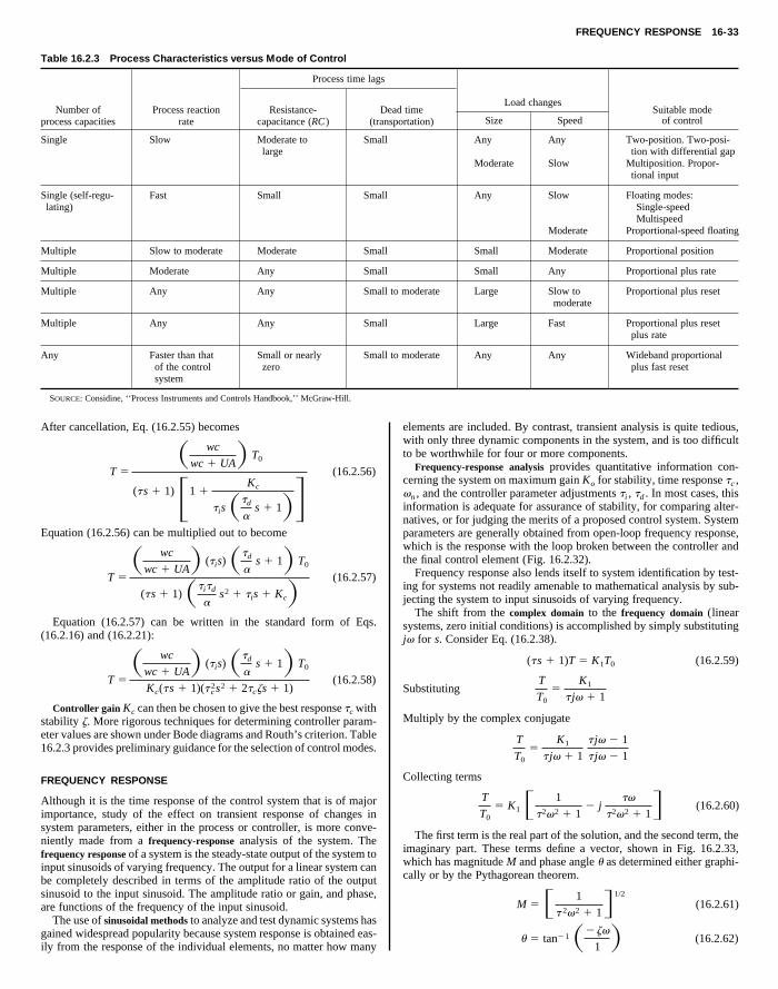
FREQUENCY RESPONSE 16-33
Table 16.2.3 Process Characteristics versus Mode of Control
Process time lags
Number of Process reaction Resistance- Dead time Suitable modeprocess capacities rate capacitance (RC ) (transportation)
Load changes
Size Speed of control
Single Slow Moderate tolarge
Small Any Any Two-position. Two-posi-tion with differential gap
Moderate Slow Multiposition. Propor-tional input
Single (self-regu-lating)
Fast Small Small Any Slow Floating modes:Single-speedMultispeed
Moderate Proportional-speed floating
Multiple Slow to moderate Moderate Small Small Moderate Proportional position
Multiple Moderate Any Small Small Any Proportional plus rate
Multiple Any Any Small to moderate Large Slow tomoderate
Proportional plus reset
Multiple Any Any Small Large Fast Proportional plus resetplus rate
Any Faster than thatof the controlsystem
Small or nearlyzero
Small to moderate Any Any Wideband proportionalplus fast reset
SOURCE: Considine, ‘‘Process Instruments and Controls Handbook,’’ McGraw-Hill.
After cancellation, Eq. (16.2.55) becomes
T 5
S wc
wc 1 UAD T0
(ts 1 1)F1 1Kc
tisStd
as 1 1DG
(16.2.56)
Equation (16.2.56) can be multiplied out to become
elements are included. By contrast, transient analysis is quite tedious,with only three dynamic components in the system, and is too difficultto be worthwhile for four or more components.
Frequency-response analysis provides quantitative information con-cerning the system on maximum gain Ko for stability, time response tc ,vn , and the controller parameter adjustments ti , td . In most cases, thisinformation is adequate for assurance of stability, for comparing alter-natives, or for judging the merits of a proposed control system. Systemparameters are generally obtained from open-loop frequency response,which is the response with the loop broken between the controller and
Copyright (C) 1999 by The McGraw-Hill Companies, Inc. All rights reserved. Use ofthis product is subject to the terms of its License Agreement. Click here to view.
T 5
S wc
wc 1 UAD (tis) Std
as 1 1D T0
(ts 1 1)Stitd
as2 1 tis 1 KcD (16.2.57)
Equation (16.2.57) can be written in the standard form of Eqs.(16.2.16) and (16.2.21):
T 5
S wc
wc 1 UAD (tis) Std
as 1 1D T0
Kc(ts 1 1)(t c2s2 1 2tczs 1 1)
(16.2.58)
Controller gain Kc can then be chosen to give the best response tc withstability z. More rigorous techniques for determining controller param-eter values are shown under Bode diagrams and Routh’s criterion. Table16.2.3 provides preliminary guidance for the selection of control modes.
FREQUENCY RESPONSE
Although it is the time response of the control system that is of majorimportance, study of the effect on transient response of changes insystem parameters, either in the process or controller, is more conve-niently made from a frequency-response analysis of the system. Thefrequency response of a system is the steady-state output of the system toinput sinusoids of varying frequency. The output for a linear system canbe completely described in terms of the amplitude ratio of the outputsinusoid to the input sinusoid. The amplitude ratio or gain, and phase,are functions of the frequency of the input sinusoid.
The use of sinusoidal methods to analyze and test dynamic systems hasgained widespread popularity because system response is obtained eas-ily from the response of the individual elements, no matter how many
the final control element (Fig. 16.2.32).Frequency response also lends itself to system identification by test-
ing for systems not readily amenable to mathematical analysis by sub-jecting the system to input sinusoids of varying frequency.
The shift from the complex domain to the frequency domain (linearsystems, zero initial conditions) is accomplished by simply substitutingjv for s. Consider Eq. (16.2.38).
(ts 1 1)T 5 K1T0 (16.2.59)
SubstitutingT
T0
5K1
t jv 1 1
Multiply by the complex conjugate
T
T0
5K1
t jv 1 1
t jv 2 1
t jv 2 1
Collecting terms
T
T0
5 K1F 1
t2v2 1 12 j
tv
t2v2 1 1G (16.2.60)
The first term is the real part of the solution, and the second term, theimaginary part. These terms define a vector, shown in Fig. 16.2.33,which has magnitude M and phase angle u as determined either graphi-cally or by the Pythagorean theorem.
M 5F 1
t 2v2 1 1G1/2
(16.2.61)
u 5 tan21S2zv
1 D (16.2.62)
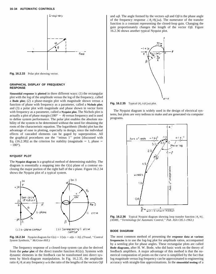
16-34 AUTOMATIC CONTROLS
and ab. The angle formed by the vectors ab and Ob is the phase angleof the frequency response /uo/ui( jv). The numerator of the transferfunction is a constant representing the closed-loop gain. Changing thegain proportionately changes the length of the vector Ob. Figure16.2.36 shows another typical Nyquist plot.
Copyright (C) 1999 by The McGraw-Hill Companies, Inc. All rights reserved. Use ofthis product is subject to the terms of its License Agreement. Click here to view.
Fig. 16.2.33 Polar plot showing vector.
GRAPHICAL DISPLAY OF FREQUENCYRESPONSE
Sinusoidal response is plotted in three different ways: (1) the rectangularplot with the log of the amplitude versus the log of the frequency, calleda Bode plot; (2) a phase-margin plot with magnitude shown versus afunction of phase with frequency as a parameter, called a Nichols plot;and (3) a polar plot with magnitude and phase shown in vector formwith frequency as a parameter, called a Nyquist plot. The Nichols plot isactually a plot of phase margin (180° 2 u) versus frequency and is usedto define system performance. The polar plot enables the absolute sta-bility of the system to be determined without the need for obtaining theroots of the characteristic equation. The logarithmic (Bode) plot has theadvantage of ease in plotting, especially in design, since the individualeffects of cascaded elements can be gaged by superposition. Allthe graphical procedures use the ‘‘minus 1’’ point [discussed withEq. (16.2.38)] as the criterion for stability (magnitude 5 1, phase 52180°).
NYQUIST PLOT
The Nyquist diagram is a graphical method of determining stability. Thediagram is essentially a mapping into the G(s) plane of a contour en-closing the major portion of the right half of the s plane. Figure 16.2.34shows the Nyquist plot of a typical system.
Fig. 16.2.34 Nyquist diagram for G(s) 5 1/[s(s 1 a)(s 1 b)]. (Truxal, ‘‘ControlSystem Synthesis,’’ McGraw-Hill.)
The frequency response of a closed-loop system can also be derivedfrom the polar plot of the direct transfer function KG(s). Systems withdynamic elements in the feedback can be transformed into direct sys-tems by block-diagram manipulation. In Fig. 16.2.35, the amplituderatio uo/ui at any frequency v is the ratio of the lengths of the vectors Ob
Fig. 16.2.35 Typical (uo /«)/( jv) plot.
The Nyquist diagram is widely used in the design of electrical sys-tems, but plots are very tedious to make and are generated via computerprograms.
Fig. 16.2.36 Typical Nyquist diagram showing loop transfer function |uo /ui |.(ASME, ‘‘Terminology for Automatic Control,’’ Pub. ASA C85.1-1963.)
BODE DIAGRAM
The most common method of presenting the response data at variousfrequencies is to use the log-log plot for amplitude ratios, accompaniedby a semilog plot for phase angles. These rectangular plots are calledBode diagrams, after H. W. Bode, who did basic work on the theory offeedback amplifiers. A major advantage of this method is that the nu-merical computation of points on the curve is simplified by the fact thatlog magnitude versus log frequency can be approximated to engineeringaccuracy with straight-line approximations. In the sinusoidal testing of a
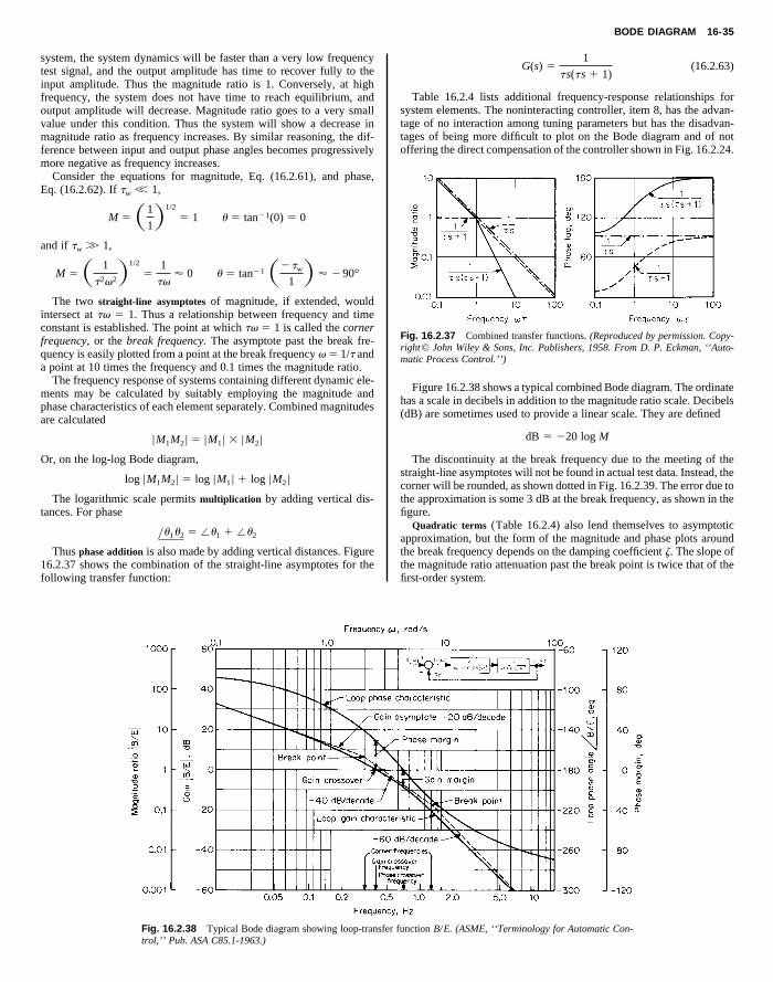
BODE DIAGRAM 16-35
system, the system dynamics will be faster than a very low frequencytest signal, and the output amplitude has time to recover fully to theinput amplitude. Thus the magnitude ratio is 1. Conversely, at highfrequency, the system does not have time to reach equilibrium, andoutput amplitude will decrease. Magnitude ratio goes to a very smallvalue under this condition. Thus the system will show a decrease inmagnitude ratio as frequency increases. By similar reasoning, the dif-ference between input and output phase angles becomes progressivelymore negative as frequency increases.
Consider the equations for magnitude, Eq. (16.2.61), and phase,
G(s) 51
ts(ts 1 1)(16.2.63)
Table 16.2.4 lists additional frequency-response relationships forsystem elements. The noninteracting controller, item 8, has the advan-tage of no interaction among tuning parameters but has the disadvan-tages of being more difficult to plot on the Bode diagram and of notoffering the direct compensation of the controller shown in Fig. 16.2.24.
Copyright (C) 1999 by The McGraw-Hill Companies, Inc. All rights reserved. Use ofthis product is subject to the terms of its License Agreement. Click here to view.
Eq. (16.2.62). If tw ,, 1,
M 5S1
1D1/2
5 1 u 5 tan21(0) 5 0
and if tw .. 1,
M 5S 1
t2v2D1/2
51
tv' 0 u 5 tan21 S2tw
1 D ' 2 90°
The two straight-line asymptotes of magnitude, if extended, wouldintersect at tv 5 1. Thus a relationship between frequency and timeconstant is established. The point at which tv 5 1 is called the cornerfrequency, or the break frequency. The asymptote past the break fre-quency is easily plotted from a point at the break frequency v 5 1/t anda point at 10 times the frequency and 0.1 times the magnitude ratio.
The frequency response of systems containing different dynamic ele-ments may be calculated by suitably employing the magnitude andphase characteristics of each element separately. Combined magnitudesare calculated
|M1M2 | 5 |M1 | 3 |M2 |
Or, on the log-log Bode diagram,
log |M1M2 | 5 log |M1 | 1 log |M2 |
The logarithmic scale permits multiplication by adding vertical dis-tances. For phase
yu1u2 5 /u1 1 /u2
Thus phase addition is also made by adding vertical distances. Figure16.2.37 shows the combination of the straight-line asymptotes for thefollowing transfer function:
Fig. 16.2.38 Typical Bode diagram showing loop-transfertrol,’’ Pub. ASA C85.1-1963.)
Fig. 16.2.37 Combined transfer functions. (Reproduced by permission. Copy-right© John Wiley & Sons, Inc. Publishers, 1958. From D. P. Eckman, ‘‘Auto-matic Process Control.’’)
Figure 16.2.38 shows a typical combined Bode diagram. The ordinatehas a scale in decibels in addition to the magnitude ratio scale. Decibels(dB) are sometimes used to provide a linear scale. They are defined
dB 5 220 log M
The discontinuity at the break frequency due to the meeting of thestraight-line asymptotes will not be found in actual test data. Instead, thecorner will be rounded, as shown dotted in Fig. 16.2.39. The error due tothe approximation is some 3 dB at the break frequency, as shown in thefigure.
Quadratic terms (Table 16.2.4) also lend themselves to asymptoticapproximation, but the form of the magnitude and phase plots aroundthe break frequency depends on the damping coefficient z. The slope ofthe magnitude ratio attenuation past the break point is twice that of thefirst-order system.
function B/E. (ASME, ‘‘Terminology for Automatic Con-
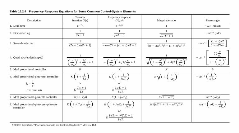
Table 16.2.4 Frequency-Response Equations for Some Common Control-System Elements
Transfer Frequency responseDescription function G (s) G ( jv) Magnitude ratio Phase angle
1. Dead time «2TLs «2j vTL 1 2 vTL radians
2. First-order lag1
Ts 1 1
1
jvT 1 1
1
√v2T2 1 12 tan21 (vT )
3. Second-order lag1
(Ts 1 1)(aTs 1 1)
1
2 av2T2 1 j (1 1 a)vT 1 1
1
√(1 2 av2T2)2 1 (1 1 a)2v2T22 tan21F (1 1 a)vT
1 2 aT2v2G
4. Quadratic (underdamped)1
S s
vnD2
12z
vn
s 1 1
1
2S v
vnD2
1 j 2zv
vn
1 1
1
√S1 2v2
vn2D2
1 4z 2S v
vnD2
2 tan21F 2zv
vn
1 2S v
vnD2G
5. Ideal proportional controller K K K 0
6. Ideal proportional-plus-reset controller
Ti 51
r
r 5 reset rate
KS1 11
TisD
or
KTis 1 1
Tis
KS1 11
j vTiD
or
Kj vTi 1 1
j vTi
K √1 1S 1
vTiD2
2 tan21S 1
vTiD
7. Ideal proportional-plus-rate controller K(1 1 Tds) K(1 1 j vTd) K √1 1 v2Td2 tan21 (vTd)
8. Ideal proportional-plus-reset-plus-ratecontroller
KS1 1 Tds 11
TisD KS1 1 j vTd 1
1
j vTiD
or
Kj vTi 2 v2TdTi 1 1
j vTi
K √(vTi)2 1 (1 2 v2TdTi)2 tan21SvTd 21
vTiD
SOURCE: Considine, ‘‘Process Instruments and Controls Handbook,’’ McGraw-Hill.
16-36
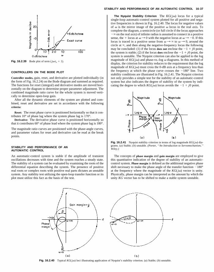
STABILITY AND PERFORMANCE OF AN AUTOMATIC CONTROL 16-37
Fig. 16.2.39 Bode plot of term ( jvta 1 1).
CONTROLLERS ON THE BODE PLOT
Controller modes, gain, reset, and derivative are plotted individually (inthe form of Fig. 16.2.24) on the Bode diagram and summed as required.The functions for reset (integral) and derivative modes are moved hori-zontally on the diagram to determine proper parameter adjustment. Thecombined magnitude ratio curve for the whole system is moved verti-cally to determine open-loop gain.
After all the dynamic elements of the system are plotted and com-bined, reset and derivative are set in accordance with the following
The Nyquist Stability Criterion The KG( jv) locus for a typicalsingle-loop automatic-control system plotted for all positive and nega-tive frequencies is shown in Fig. 16.2.40. The locus for negative valuesof v is the mirror image of the positive v locus in the real axis. Tocomplete the diagram, a semicircle (or full circle if the locus approaches2` on the real axis) of infinite radius is assumed to connect in a positivesense, the 1 locus at v : 0 with the negative locus at v : 20. If thislocus is traced in a positive sense from v : ` to v : 0, around thecircle at `, and then along the negative-frequency locus the followingmay be concluded: (1) if the locus does not enclose the 21 1 j0 point,
Copyright (C) 1999 by The McGraw-Hill Companies, Inc. All rights reserved. Use ofthis product is subject to the terms of its License Agreement. Click here to view.
criteria:
Reset: The reset phase curve is positioned horizontally so that it con-tributes 10° of phase lag where the system phase lag is 170°.
Derivative: The derivative phase curve is positioned horizontally sothat it contributes 60° of phase lead where the system phase lag is 180°.
The magnitude ratio curves are positioned with the phase-angle curves,and parameter values for reset and derivative can be read at the breakpoints.
STABILITY AND PERFORMANCE OF ANAUTOMATIC CONTROL
An automatic-control system is stable if the amplitude of transientoscillations decreases with time and the system reaches a steady state.The stability of a system can be evaluated by examining the roots of thedifferential equation describing the system. The presence of positivereal roots or complex roots with positive real parts dictates an unstablesystem. Any stability test utilizing the open-loop transfer function or itsplot must utilize this fact as the basis of the test.
Fig. 16.2.40 Typical KG( jv) loci illustrating application o
the system is stable; (2) if the locus does enclose the 21 1 j0 point, thesystem is unstable. The Nyquist criterion can also be applied to the logmagnitude of KG( jv) and phase-vs.-log v diagrams. In this method ofdisplay, the criterion for stability reduces to the requirement that the logmagnitude of KG( jv) must cross the 0-dB axis at a frequency less thanthe frequency at which the phase curve crosses the 2180° line. Twostability conditions are illustrated in Fig. 16.2.41. The Nyquist criterionnot only provides a simple test for the stability of an automatic-controlsystem but also indicates the degree of stability of the system by indi-cating the degree to which KG( jv) locus avoids the 21 1 j0 point.
Fig. 16.2.41 Nyquist stability criterion in terms of log magnitude KG( jv) dia-grams. (a) Stable; (b) unstable. (Porter, ‘‘An Introduction to Servomechanism,’’Wiley.)
The concepts of phase margin and gain margin are employed to givethis quantitative indication of the degree of stability of an automatic-control system. Phase margin is defined as the additional negative phaseshift necessary to make the phase angle of the transfer function 2180°at the frequency where the magnitude of the KG( jv) vector is unity.Physically, phase margin can be interpreted as the amount by which theunity KG vector has to be shifted to make a stable system unstable.
f Nyquist’s stability criterion. (a) Stable; (b) unstable.
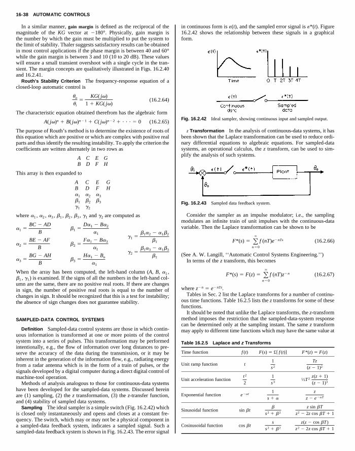
16-38 AUTOMATIC CONTROLS
In a similar manner, gain margin is defined as the reciprocal of themagnitude of the KG vector at 2180°. Physically, gain margin isthe number by which the gain must be multiplied to put the system tothe limit of stability. Thaler suggests satisfactory results can be obtainedin most control applications if the phase margin is between 40 and 60°while the gain margin is between 3 and 10 (10 to 20 dB). These valueswill ensure a small transient overshoot with a single cycle in the tran-sient. The margin concepts are qualitatively illustrated in Figs. 16.2.40and 16.2.41.
Routh’s Stability Criterion The frequency-response equation of a
in continuous form is «(t), and the sampled error signal is «*(t). Figure16.2.42 shows the relationship between these signals in a graphicalform.
Copyright (C) 1999 by The McGraw-Hill Companies, Inc. All rights reserved. Use ofthis product is subject to the terms of its License Agreement. Click here to view.
closed-loop automatic control is
uo
ui
5KG( jv)
1 1 KG( jv)(16.2.64)
The characteristic equation obtained therefrom has the algebraic form
A( jv)n 1 B( jv)n21 1 C( jv)n22 1 ? ? ? 5 0 (16.2.65)
The purpose of Routh’s method is to determine the existence of roots ofthis equation which are positive or which are complex with positive realparts and thus identify the resulting instability. To apply the criterion thecoefficients are written alternately in two rows as
A C E GB D F H
This array is then expanded to
A C E GB D F Ha1 a2 a3
b1 b2 b3
g1 g2
where a1 , a2 , a3 , b1 , b2 , b3 , g1 and g2 are computed as
a1 5BC 2 AD
B
a2 5BE 2 AF
B
a3 5BG 2 AH
B
b1 5Da1 2 Ba2
a1
b2 5Fa1 2 Ba3
a1
b3 5Ha1 2 Bo
a1
g1 5b1a2 2 a1b2
b1
g2 5b1a3 2 a1b3
b1
When the array has been computed, the left-hand column (A, B, a1 ,b1 , g1) is examined. If the signs of all the numbers in the left-hand col-umn are the same, there are no positive real roots. If there are changesin sign, the number of positive real roots is equal to the number ofchanges in sign. It should be recognized that this is a test for instability;the absence of sign changes does not guarantee stability.
SAMPLED-DATA CONTROL SYSTEMS
Definition Sampled-data control systems are those in which contin-uous information is transformed at one or more points of the controlsystem into a series of pulses. This transformation may be performedintentionally, e.g., the flow of information over long distances to pre-serve the accuracy of the data during the transmission, or it may beinherent in the generation of the information flow, e.g., radiating energyfrom a radar antenna which is in the form of a train of pulses, or thesignals developed by a digital computer during a direct digital control ofmachine-tool operation.
Methods of analysis analogous to those for continuous-data systemshave been developed for the sampled-data systems. Discussed hereinare (1) sampling, (2) the z transformation, (3) the z-transfer function,and (4) stability of sampled data systems.
Sampling The ideal sampler is a simple switch (Fig. 16.2.42) whichis closed only instantaneously and opens and closes at a constant fre-quency. The switch, which may or may not be a physical component ina sampled-data feedback system, indicates a sampled signal. Such asampled-data feedback system is shown in Fig. 16.2.43. The error signal
Fig. 16.2.42 Ideal sampler, showing continuous input and sampled output.
z Transformation In the analysis of continuous-data systems, it hasbeen shown that the Laplace transformation can be used to reduce ordi-nary differential equations to algebraic equations. For sampled-datasystems, an operational calculus, the z transform, can be used to sim-plify the analysis of such systems.
Fig. 16.2.43 Sampled data feedback system.
Consider the sampler as an impulse modulator; i.e., the samplingmodulates an infinite train of unit impulses with the continuous-datavariable. Then the Laplace transformation can be shown to be
F*(s) 5 O`n50
f (nT)e2nTs (16.2.66)
(See A. W. Langill, ‘‘Automatic Control Systems Engineering.’’)In terms of the z transform, this becomes
F*(s) 5 F(z) 5 O`n50
f (nT)z2n (16.2.67)
where z2n 5 e2nTs.Tables in Sec. 2 list the Laplace transforms for a number of continu-
ous time functions. Table 16.2.5 lists the z transforms for some of thesefunctions.
It should be noted that unlike the Laplace transforms, the z-transformmethod imposes the restriction that the sampled-data-system responsecan be determined only at the sampling instant. The same z transformmay apply to different time functions which may have the same value at
Table 16.2.5 Laplace and z Transforms
Time function f (t) F(s) 5 £[ f (t)] F*(z) 5 F (z)
Unit ramp function t1
s2
Tz
(z 2 1)2
Unit acceleration functiont2
2
1
s31⁄2T2
z(z 1 1)
(z 2 1)3
Exponential function e2at1
s 1 a
z
z 2 e2aT
Sinusoidal function sin btb
s2 1 b2
z sin bT
z2 2 2z cos bT 1 1
Cosinusoidal function cos bts
s2 1 b2
z(z 2 cos bT )
z2 2 2z cos bT 1 1
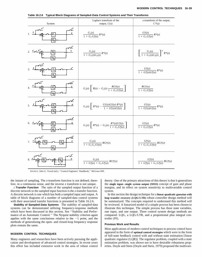
MODERN CONTROL TECHNIQUES 16-39
Table 16.2.6 Typical Block Diagrams of Sampled-Data Control Systems and Their Transforms
Laplace transform of the z-transform of the output,System output, C(s) C*(z)
1. G1(s)
1 1 G1G2*(z)R*(z)
G1*(z)
1 1 G1G2*(z)R*(z)
2. G1(s)
1 1 G1(s)G2(s)R*(z) F G1(s)
1 1 G1(s)G2(s)G*R*(z)
3. G1*(z)
1 1 G1*(z)G2*(z)R*(z)
4. G1(s)FR(s) 2 G2(s)RG1*(z)
1 1 G1G2*(z)G RG1*(s)
1 1 G1G2*(s)
5. G1(s)FR*(z) 2G1*(z)G2*(z) R*(z)
1 1 G1*(z)G2*(z) G G1*(z)
1 1 G1*(z)G2*(z)R*(z)
6.G1(s)FR*(z) 2 G2(s)
R*(z)G1*(z)
1 1 G1G2*(z)G G1*(z)
1 1 G1G2*(z)R*(z)
7. G2(s)
1 1 G1G2G3*(z)RG1*(z)
G2*(z)
1 1 G1G2G3*(z)RG1*(z)
8. G2(s)
1 1 G2*(z) 1 G1G2*(z)RG1*(z)
G2*(z)
1 1 G2*(z) 1 G1G2*(z)RG1*(z)
SOURCE: John G. Truxal (ed.), ‘‘Control Engineers’ Handbook,’’ McGraw-Hill.
the instant of sampling. The z-transform function is not defined, there-fore, in a continuous sense, and the inverse z transform is not unique.
z Transfer Function The ratio of the sampled output function of adiscrete network to the sampled input function is the z-transfer function.A discrete network is one which has both a sampled input and output. Atable of block diagrams of a number of sampled-data control systemswith their associated transfer functions is presented in Table 16.2.6.
Stability of Sampled-Data Systems The stability of sampled-datasystems can be demonstrated utilizing frequency-response methodswhich have been discussed in this section. See ‘‘Stability and Perfor-
theory. One of the primary attractions of this theory is that it generalizesthe single input–single system output (SISO) concept of gain and phasemargins, and its effect on system sensitivity to multivariable controlsystem.
In this section the design technique for a linear quadratic gaussian withloop transfer recovery (LQG/LTR) robust controller design method willbe summarized. The concepts required to understand this method willbe reviewed. A linearized model of a simple process has been chosen toillustrate this technique. The simple process has three state variables,one input, and one output. Three control system design methods are
Copyright (C) 1999 by The McGraw-Hill Companies, Inc. All rights reserved. Use ofthis product is subject to the terms of its License Agreement. Click here to view.
mance of an Automatic Control.’’ The Nyquist stability criterion againapplies with the same conclusions relative to the 21 point, and themethods of generalizing the open- and closed-loop frequency responseplots remain the same.
MODERN CONTROL TECHNIQUES
Many engineers and researchers have been actively pursuing the appli-cation and development of advanced control strategies. In recent yearsthis effort has included extensive work in the area of robust control
compared: LQG, a LQG/LTR, and a proportional plus integral con-troller (PI).
Previous Work and Results
Most applications of modern control techniques to process control haveappeared in the form of optimal control strategies which were in the formof full-state feedback control with and without state estimation [linearquadratic regulator (LQR)]. The regulator problem, coupled with a stateestimation problem, was shown not to have desirable robustness prop-erties. Doyle and Stein (Doyle and Stein, 1979) proposed the multivari-
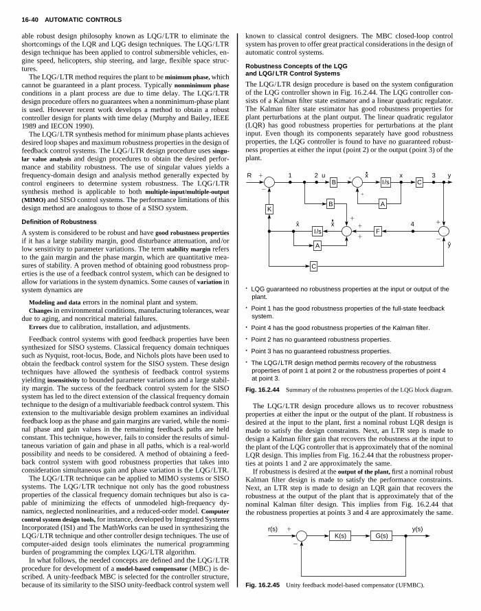
16-40 AUTOMATIC CONTROLS
able robust design philosophy known as LQG/LTR to eliminate theshortcomings of the LQR and LQG design techniques. The LQG/LTRdesign technique has been applied to control submersible vehicles, en-gine speed, helicopters, ship steering, and large, flexible space struc-tures.
The LQG/LTR method requires the plant to be minimum phase, whichcannot be guaranteed in a plant process. Typically nonminimum phaseconditions in a plant process are due to time delay. The LQG/LTRdesign procedure offers no guarantees when a nonminimum-phase plantis used. However recent work develops a method to obtain a robust
known to classical control designers. The MBC closed-loop controlsystem has proven to offer great practical considerations in the design ofautomatic control systems.
Robustness Concepts of the LQGand LQG/LTR Control Systems
The LQG/LTR design procedure is based on the system configurationof the LQG controller shown in Fig. 16.2.44. The LQG controller con-sists of a Kalman filter state estimator and a linear quadratic regulator.The Kalman filter state estimator has good robustness properties for
·
·
····
Copyright (C) 1999 by The McGraw-Hill Companies, Inc. All rights reserved. Use ofthis product is subject to the terms of its License Agreement. Click here to view.
controller design for plants with time delay (Murphy and Bailey, IEEE1989 and IECON 1990).
The LQG/LTR synthesis method for minimum phase plants achievesdesired loop shapes and maximum robustness properties in the design offeedback control systems. The LQG/LTR design procedure uses singu-lar value analysis and design procedures to obtain the desired perfor-mance and stability robustness. The use of singular values yields afrequency-domain design and analysis method generally expected bycontrol engineers to determine system robustness. The LQG/LTRsynthesis method is applicable to both multiple-input/multiple-output(MIMO) and SISO control systems. The performance limitations of thisdesign method are analogous to those of a SISO system.
Definition of Robustness
A system is considered to be robust and have good robustness propertiesif it has a large stability margin, good disturbance attenuation, and/orlow sensitivity to parameter variations. The term stability margin refersto the gain margin and the phase margin, which are quantitative mea-sures of stability. A proven method of obtaining good robustness prop-erties is the use of a feedback control system, which can be designed toallow for variations in the system dynamics. Some causes of variation insystem dynamics are
Modeling and data errors in the nominal plant and system.Changes in environmental conditions, manufacturing tolerances, wear
due to aging, and noncritical material failures.Errors due to calibration, installation, and adjustments.
Feedback control systems with good feedback properties have beensynthesized for SISO systems. Classical frequency domain techniquessuch as Nyquist, root-locus, Bode, and Nichols plots have been used toobtain the feedback control system for the SISO system. These designtechniques have allowed the synthesis of feedback control systemsyielding insensitivity to bounded parameter variations and a large stabil-ity margin. The success of the feedback control system for the SISOsystem has led to the direct extension of the classical frequency domaintechnique to the design of a multivariable feedback control system. Thisextension to the multivariable design problem examines an individualfeedback loop as the phase and gain margins are varied, while the nomi-nal phase and gain values in the remaining feedback paths are heldconstant. This technique, however, fails to consider the results of simul-taneous variation of gain and phase in all paths, which is a real-worldpossibility and needs to be considered. A method of obtaining a feed-back control system with good robustness properties that takes intoconsideration simultaneous gain and phase variation is the LQG/LTR.
The LQG/LTR technique can be applied to MIMO systems or SISOsystems. The LQG/LTR technique not only has the good robustnessproperties of the classical frequency domain techniques but also is ca-pable of minimizing the effects of unmodeled high-frequency dy-namics, neglected nonlinearities, and a reduced-order model. Computercontrol system design tools, for instance, developed by Integrated SystemsIncorporated (ISI) and The MathWorks can be used in synthesizing theLQG/LTR technique and other controller design techniques. The use ofcomputer-aided design tools eliminates the numerical programmingburden of programming the complex LQG/LTR algorithm.
In what follows, the needed concepts are defined and the LQG/LTRprocedure for development of a model-based compensator (MBC) is de-scribed. A unity-feedback MBC is selected for the controller structure,because of its similarity to the SISO unity-feedback control system well
plant perturbations at the plant output. The linear quadratic regulator(LQR) has good robustness properties for perturbations at the plantinput. Even though its components separately have good robustnessproperties, the LQG controller is found to have no guaranteed robust-ness properties at either the input (point 2) or the output (point 3) of theplant.
RB
A
A
C
LQG guaranteed no robustness properties at the input or output of the plant.
Point 1 has the good robustness properties of the full-state feedback system.
Point 4 has the good robustness properties of the Kalman filter.
Point 2 has no guaranteed robustness properties.
Point 3 has no guaranteed robustness properties.
The LQG/LTR design method permits recovery of the robustness properties of point 1 at point 2 or the robustness properties of point 4 at point 3.
BK
I/s
I /s F
C1 2 3
4
1
2
1
1
1
11
21
u x x y
y
xx
ˆ
Fig. 16.2.44 Summary of the robustness properties of the LQG block diagram.
The LQG/LTR design procedure allows us to recover robustnessproperties at either the input or the output of the plant. If robustness isdesired at the input to the plant, first a nominal robust LQR design ismade to satisfy the design constraints. Next, an LTR step is made todesign a Kalman filter gain that recovers the robustness at the input tothe plant of the LQG controller that is approximately that of the nominalLQR design. This implies from Fig. 16.2.44 that the robustness proper-ties at points 1 and 2 are approximately the same.
If robustness is desired at the output of the plant, first a nominal robustKalman filter design is made to satisfy the performance constraints.Next, an LTR step is made to design an LQR gain that recovers therobustness at the output of the plant that is approximately that of thenominal Kalman filter design. This implies from Fig. 16.2.44 thatthe robustness properties at points 3 and 4 are approximately the same.
r(s) y(s)G(s)K(s)
1
2
Fig. 16.2.45 Unity feedback model-based compensator (UFMBC).
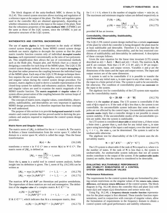
STABILITY ROBUSTNESS 16-41
The block diagram of the unity-feedback MBC is shown in Fig.16.2.45. This control system structure allows tracking and regulation ofa reference input at the output of the plant. The filter and regulator gainsused in the controller R(s) are obtained appropriately, depending onwhether robustness is desired at the input or the output of the plant. Notethat the robustness properties of the unity-feedback MBC (UFMBC) arethe same as those of the LQG system, since the UFMBC is just analternative structure of the LQG system.
for 1 # i # k, where k is the number of singular values 5 min (m, n).The maximum and minimum singular values are defined respectively as
s (A) 5 ||A||2 (16.2.74)
and s (A) 5 maxxÞ0
||Ax||
||x ||25
1||A21||2
(16.2.75)
provided A has an inverse.
Controllability, Observability, Stabilizability,and Detectability
Copyright (C) 1999 by The McGraw-Hill Companies, Inc. All rights reserved. Use ofthis product is subject to the terms of its License Agreement. Click here to view.
MATHEMATICS AND CONTROL BACKGROUND
The use of matrix algebra is very important in the study of MIMOcontrol system design methods. Some MIMO control system designmethods use matrix algebra to decouple the system so that the plantmatrix transfer function consists only of individual decoupled transferfunctions, each represented conventionally as the ratio of two polynomi-als. This simplification then allows the use of conventional methodssuch as the Bode plot, Nyquist plot, and Nichols chart as a means ofdesigning a controller for each loop of the MIMO plant. The LQG/LTRcontrol system design method, however, does not require decoupling ofthe plant but rather preserves the coupling between the individual loopsof the MIMO plant. Each step of the LQG/LTR design technique there-fore requires the use of some matrix algebra, vector and matrix norms,and singular values during the control system design procedure. Forinstance, matrix algebra is used to derive a suitable representation of theclosed-loop system for stability and robustness analysis. Matrix normsand singular values are used to examine the matrix magnitude of theMIMO transfer function. The matrix magnitude or singular values of asystem allows preservation of the coupling between the various loops ofthe MIMO control system.
The concepts of matrix norm, singular values, controllability, observ-ability, stabilizability, and detectability are very important in applyingMIMO design procedures. It is therefore important that these conceptsbe well understood.
The purpose of this section is to provide background material in math-ematics and control systems that has proved useful in deriving the pro-cedures and analysis required to implement the control system designprocedure.
Matrix Norm and Singular Values
The matrix norm of ||A||2 is defined for the m 3 n matrix A. The matrixA defines a linear transformation from the vector space V, called thedomain to a vector space W, which is called the range. Thus the lineartransformation
A(x) 5 Ax (16.2.68)
transforms a vector x in V [ Cn into a vector A(x) in W [ Cm. Thematrix norm of ||A||2 is defined as
||A||2 5 maxxÞ0
||A||2||x ||2
5 l2 norm (16.2.69)
Since the l2 norm is a useful tool in control system analysis, furtherinsight into its definition is given. The l2 norm of Eq. (16.2.69) can bewritten as
||A||2 5 maxi
[li(AHA)]1/2 i 5 1, 2, ? ? ? , n (16.2.70)
||A||2 5 maxi
[li(AAH)]1/2 i 5 1, 2, ? ? ? , n (16.2.71)
The matrices AHA and AAH are Hermitian and positive semidefinite.The eigenvalues of these matrices are real and nonnegative. The defini-tion of the singular value of a complex matrix A [ Cn3n is
si (A) 5 [li(AHA)]1/2
5 [li(AAH)]1/2 $ 0 i 5 1, 2, ? ? ? , n (16.2.72)
If A [ Cm3n, which indicates that A is a nonsquare matrix, then
si (A) 5 [li(AHA)]1/2 5 [li(AAH)]1/2 (16.2.73)
The LQG/LTR control system design method has a certain requirementof the plant for which the controller is being designed: the plant must beat least stabilizable and detectable. Therefore it is important that theconditions of controllability, observability, and the less restricted con-ditions of stabilizability and detectability be understood. A descriptionof these concepts follows.
Given the state equation for the linear time invariant (LTI) systemdescribed as ~x(t) 5 Ax(t) 1 Bu(t) and y(t) 5 Cx(t). The matrices A, B,and C are constant. Note that x [ Rn, n [ Rp, and y [ Rp are respec-tively the state, input, and output vectors. Variables n and p are thedimensions of the states and the input and output vectors. The input andoutput vectors are of the same dimension.
A system is said to be controllable if it is possible to transfer thesystem from any initial state x0 in state space to any other state xF usingthe input in a finite period of time. The system is said to be uncontrolla-ble otherwise. The condition of controllability places no constraint onthe input in the system.
The algebraic test for controllability of the LTI system state equationuses the controllability matrix
Q 5 [B AB ? ? ? An21B] (16.2.76)
where n is the number of states. The LTI system is controllable if therank of Q is equal to n. If the rank of Q is less than n, the system is notcontrollable. An uncontrollable system indicates that some modes orpoles are not affected by the control input. Uncontrollable systems withunstable modes imply that a controller design is not possible to ensuresystem stability. If the uncontrollable modes of the uncontrollable sys-tem are stable, then the system is stabilizable.
An LTI system is considered observable at initial time t0 if there existsa finite time t1 greater than t0 such that for any initial state x0 in statespace using knowledge of the input u and output y over the time intervalt0 , t , t1 , the state x0 can be determined. The system is said to beunobservable otherwise.
The algebraic test for observability of the LTI system uses the ob-servability matrix
N 5 [CT ATCT ? ? ? (AT)n21CT] (16.2.77)
The LTI system is observable if the rank of N is equal to n, where n isthe number of states. If the rank of N is less than n, the system isunobservable. An unobservable system indicates that not all systemmodes contribute to the output of the system. If the unobservable modes(states) are stable, then the system is considered to be detectable.
EVALUATING MULTIVARIABLE PERFORMANCEAND STABILITY ROBUSTNESS OF A CONTROLSYSTEM USING SINGULAR VALUES
Performance Robustness
The requirements for the control system design are formulated by plac-ing certain restrictions on the singular values of the return ratio, returndifference, and inverse return difference of the control system. The blockdiagram in Fig. 16.2.46 shows the controller K(s) and plant G(s) withinput dI(s) and output do(s) disturbances and sensor noise n(s).
Using Fig. 16.2.46, a frequency-domain transfer function representa-tion for the plant output is first obtained. These transfer function repre-sentations, used in conjunction with concepts of singular values, allowthe formulation of requirements in the frequency domain to obtain acontrol system with good performance and stability robustness.
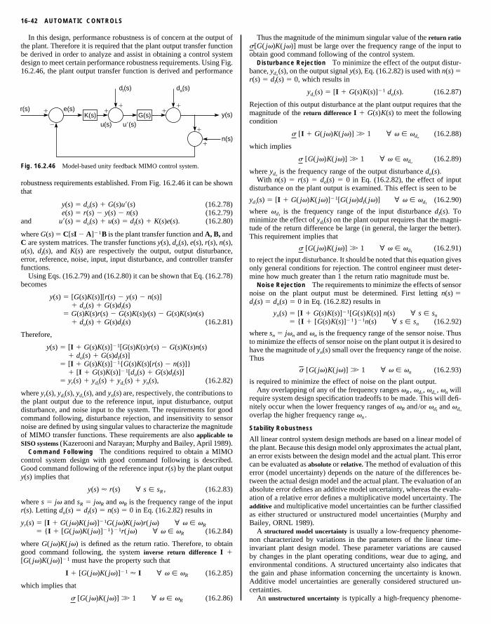
16-42 AUTOMATIC CONTROLS
In this design, performance robustness is of concern at the output ofthe plant. Therefore it is required that the plant output transfer functionbe derived in order to analyze and assist in obtaining a control systemdesign to meet certain performance robustness requirements. Using Fig.16.2.46, the plant output transfer function is derived and performance
r(s)
dI(s) do(s)
e(s)1 11
11
Thus the magnitude of the minimum singular value of the return ratios[G( jv)K( jv)] must be large over the frequency range of the input toobtain good command following of the control system.
Disturbance Rejection To minimize the effect of the output distur-bance, ydo
(s), on the output signal y(s), Eq. (16.2.82) is used with n(s) 5r(s) 5 dI(s) 5 0, which results in
ydo(s) 5 [I 1 G(s)K(s)]21 do(s). (16.2.87)
Rejection of this output disturbance at the plant output requires that themagnitude of the return difference I 1 G(s)K(s) to meet the followingc
w
w
d
y
wmtT
tom
nd
wthT
i
rno
S
AtacetaaaaB
nibetAc
n(s)
y(s)K(s) G(s)u(s) u9(s)2
1
1
Fig. 16.2.46 Model-based unity feedback MIMO control system.
robustness requirements established. From Fig. 16.2.46 it can be shownthat
y(s) 5 do(s) 1 G(s)u9(s) (16.2.78)e(s) 5 r(s) 2 y(s) 2 n(s) (16.2.79)
and u9(s) 5 do(s) 1 u(s) 5 dI(s) 1 K(s)e(s). (16.2.80)
where G(s) 5 C[sI 2 A]21B is the plant transfer function and A, B, andC are system matrices. The transfer functions y(s), do(s), e(s), r(s), n(s),u(s), dI(s), and K(s) are respectively the output, output disturbance,error, reference, noise, input, input disturbance, and controller transferfunctions.
Using Eqs. (16.2.79) and (16.2.80) it can be shown that Eq. (16.2.78)becomes
y(s) 5 [G(s)K(s)][r(s) 2 y(s) 2 n(s)]1 do(s) 1 G(s)dI(s)
5 G(s)K(s)r(s) 2 G(s)K(s)y(s) 2 G(s)K(s)n(s)1 do(s) 1 G(s)dI(s) (16.2.81)
Therefore,
y(s) 5 [I 1 G(s)K(s)]21[G(s)K(s)r(s) 2 G(s)K(s)n(s)1 do(s) 1 G(s)dI(s)]
5 [I 1 G(s)K(s)]21{G(s)K(s)[r(s) 2 n(s)]}1 [I 1 G(s)K(s)]21[do(s) 1 G(s)dI(s)]
5 yr(s) 1 ydI(s) 1 ydo
(s) 1 yn(s), (16.2.82)
where yr(s), ydI(s), ydo
(s), and yn(s) are, respectively, the contributions tothe plant output due to the reference input, input disturbance, outputdisturbance, and noise input to the system. The requirements for goodcommand following, disturbance rejection, and insensitivity to sensornoise are defined by using singular values to characterize the magnitudeof MIMO transfer functions. These requirements are also applicable toSISO systems (Kazerooni and Narayan; Murphy and Bailey, April 1989).
Command Following The conditions required to obtain a MIMOcontrol system design with good command following is described.Good command following of the reference input r(s) by the plant outputy(s) implies that
y(s) ' r(s) ∀ s [ sR , (16.2.83)
where s 5 jv and sR 5 jvR and vR is the frequency range of the inputr(s). Letting do(s) 5 dI(s) 5 n(s) 5 0 in Eq. (16.2.82) results in
yr(s) 5 [I 1 G( jv)K( jv)]21G( jv)K( jv)r( jv) ∀ v [ vR
5 {I 1 [G( jv)K( jv)]21}21r( jv) ∀ v [ vR (16.2.84)
where G( jv)K( jv) is defined as the return ratio. Therefore, to obtaingood command following, the system inverse return difference I 1[G( jv)K( jv)]21 must have the property such that
I 1 [G( jv)K( jv)]21 ' I ∀ v [ vR (16.2.85)
which implies that
s [G( jv)K( jv)] .. 1 ∀ v [ vR (16.2.86)
ondition
s [I 1 G( jv)K( jv)] .. 1 ∀ v [ vdo(16.2.88)
hich implies
s [G( jv)K( jv)] .. 1 ∀ v [ vdo(16.2.89)
here ydois the frequency range of the output disturbance do(s).
With n(s) 5 r(s) 5 do(s) 5 0 in Eq. (16.2.82), the effect of inputisturbance on the plant output is examined. This effect is seen to be
dI(s) 5 [I 1 G( jv)K( jv)]21[G( jv)dI( jv)] ∀ v [ vdI
(16.2.90)
here vdIis the frequency range of the input disturbance dI(s). To
inimize the effect of ydI(s) on the plant output requires that the magni-
ude of the return difference be large (in general, the larger the better).his requirement implies that
s [G( jv)K( jv)] .. 1 ∀ v [ vdI(16.2.91)
o reject the input disturbance. It should be noted that this equation givesnly general conditions for rejection. The control engineer must deter-ine how much greater than 1 the return ratio magnitude must be.Noise Rejection The requirements to minimize the effects of sensor
oise on the plant output must be determined. First letting n(s) 5
I(s) 5 do(s) 5 0 in Eq. (16.2.82) results in
yn(s) 5 [I 1 G(s)K(s)]21[G(s)K(s)] n(s) ∀ s [ sn
5 {I 1 [G(s)K(s)]21}21n(s) ∀ s [ sn (16.2.92)
here sn 5 jvn and vn is the frequency range of the sensor noise. Thuso minimize the effects of sensor noise on the plant output it is desired toave the magnitude of yn(s) small over the frequency range of the noise.hus
s [G( jv)K( jv)] .. 1 ∀ v [ vn (16.2.93)
s required to minimize the effect of noise on the plant output.Any overlapping of any of the frequency ranges vR , vdI
, vdo, vn will
equire system design specification tradeoffs to be made. This will defi-itely occur when the lower frequency ranges of vR and/or vdI
and vdo
verlap the higher frequency range vn .
tability Robustness
ll linear control system design methods are based on a linear model ofhe plant. Because this design model only approximates the actual plant,n error exists between the design model and the actual plant. This erroran be evaluated as absolute or relative. The method of evaluation of thisrror (model uncertainty) depends on the nature of the differences be-ween the actual design model and the actual plant. The evaluation of anbsolute error defines an additive model uncertainty, whereas the evalu-tion of a relative error defines a multiplicative model uncertainty. Thedditive and multiplicative model uncertainties can be further classifieds either structured or unstructured model uncertainties (Murphy andailey, ORNL 1989).A structured model uncertainty is usually a low-frequency phenome-
on characterized by variations in the parameters of the linear time-nvariant plant design model. These parameter variations are causedy changes in the plant operating conditions, wear due to aging, andnvironmental conditions. A structured uncertainty also indicates thathe gain and phase information concerning the uncertainty is known.dditive model uncertainties are generally considered structured un-
ertainties.An unstructured uncertainty is typically a high-frequency phenome-
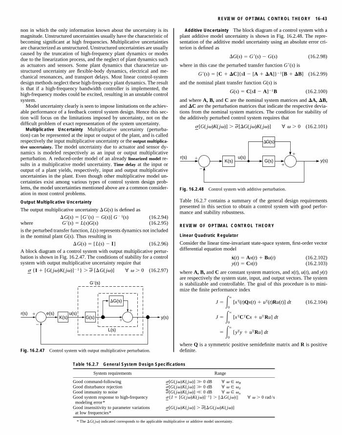
REVIEW OF OPTIMAL CONTROL THEORY 16-43
non in which the only information known about the uncertainty is itsmagnitude. Unstructured uncertainties usually have the characteristic ofbecoming significant at high frequencies. Multiplicative uncertaintiesare characterized as unstructured. Unstructured uncertainties are usuallycaused by the truncation of high-frequency plant dynamics or modesdue to the linearization process, and the neglect of plant dynamics suchas actuators and sensors. Some plant dynamics that characterize un-structured uncertainty are flexible-body dynamics, electrical and me-chanical resonances, and transport delays. Most linear control-systemdesign methods neglect these high-frequency plant dynamics. The result
Additive Uncertainty The block diagram of a control system with aplant additive model uncertainty is shown in Fig. 16.2.48. The repre-sentation of the additive model uncertainty using an absolute error cri-terion is defined as
DG(s) 5 G9(s) 2 G(s) (16.2.98)
where in this case the perturbed transfer function G9(s) is
G9(s) 5 [C 1 DC]{sI 2 [A 1 DA]}21[B 1 DB] (16.2.99)
ca
G(G(G(I 1
G(
is that if a high-frequency bandwidth controller is implemented, thehigh-frequency modes could be excited, resulting in an unstable controlsystem.
Model uncertainty clearly is seen to impose limitations on the achiev-able performance of a feedback control system design. Hence this sec-tion will focus on the limitations imposed by uncertainty, not on thedifficult problem of exact representation of the system uncertainty.
Multiplicative Uncertainty Multiplicative uncertainty (perturba-tion) can be represented at the input or output of the plant, and is calledrespectively the input multiplicative uncertainty or the output multiplica-tive uncertainty. The model uncertainty due to actuator and sensor dy-namics is modeled respectively as an input or output multiplicativeperturbation. A reduced-order model of an already linearized model re-sults in a multiplicative model uncertainty. Time delay at the input oroutput of a plant yields, respectively, input and output multiplicativeuncertainties in the plant. Even though other multiplicative model un-certainties exist among various types of control system design prob-lems, the model uncertainties mentioned above are a common consider-ation in most control problems.
Output Multiplicative Uncertainty
The output multiplicative uncertainty DG(s) is defined as
DG(s) 5 [G9(s) 2 G(s)] G21(s) (16.2.94)where G9(s) 5 L(s)G(s) (16.2.95)
is the perturbed transfer function, L(s) represents dynamics not includedin the nominal plant G(s). Thus resulting in
DG(s) 5 [L(s) 2 I] (16.2.96)
A block diagram of a control system with output multiplicative pertur-bation is shown in Fig. 16.2.47. The conditions of stability for a controlsystem with output multiplicative uncertainty require that
s {I 1 [G( jv)K( jv)]21} . s [DG( jv)] ∀ v . 0 (16.2.97)
1
2
1
1
r(s) e(s) u(s)K(s) G(s) y(s)
G9(s)
L(s)
DG(s)
Fig. 16.2.47 Control system with output multiplicative perturbation.
Table 16.2.7 General System Design Specifi
System requirements
Good command-following s[Good disturbance rejection s[Good immunity to noise s[Good system response to high-frequencymodeling error*
s{
Good insensitivity to parameter variations s[
at low frequencies** The DG( jv) indicated corresponds to the applicable multipli
and the nominal plant transfer function G(s) is
G(s) 5 C[sI 2 A]21B (16.2.100)
and where A, B, and C are the nominal system matrices and DA, DB,and DC are the perturbation matrices that indicate the respective devia-tions from the nominal system matrices. The condition for stability ofthe additively perturbed control system requires that
s [G( jv)K( jv)] . s [DG( jv)K( jv)] ∀ v . 0 (16.2.101)
r(s) u(s)y(s)K(s) G(s)
DG(s)
1
1
1
2
Fig. 16.2.48 Control system with additive perturbation.
Table 16.2.7 contains a summary of the general design requirementspresented in this section to obtain a control system with good perfor-mance and stability robustness.
REVIEW OF OPTIMAL CONTROL THEORY
Linear Quadratic Regulator
Consider the linear time-invariant state-space system, first-order vectordifferential equation model
~x(t) 5 Ax(t) 1 Bu(t) (16.2.102)y(t) 5 Cx(t) (16.2.103)
where A, B, and C are constant system matrices, and x(t), u(t), and y(t)are respectively the system state, input, and output vectors. The systemis stabilizable and controllable. The goal of this procedure is to mini-mize the finite performance index
J 5 E`
0
[xT(t)Qx(t) 1 uT(t)Ru(t)] dt (16.2.104)
J 5 E`
0
[xTCTCx 1 uTRu] dt
5 E`
0
[yTy 1 uTRu] dt
where Q is a symmetric positive semidefinite matrix and R is positivedefinite.
tions
Range
jv)K( jv)] .. 0 dB ∀ v [ vR
jv)K( jv)] .. 0 dB ∀ v [ vd
jv)K( jv)] ,, 0 dB ∀ v [ vn
[G( jv)K( jv)]21} . ||DG( jv) || ∀ v . 0 rad/s
jv)K( jv)] . s[DG( jv)K( jv)]
cative or additive model uncertainty.
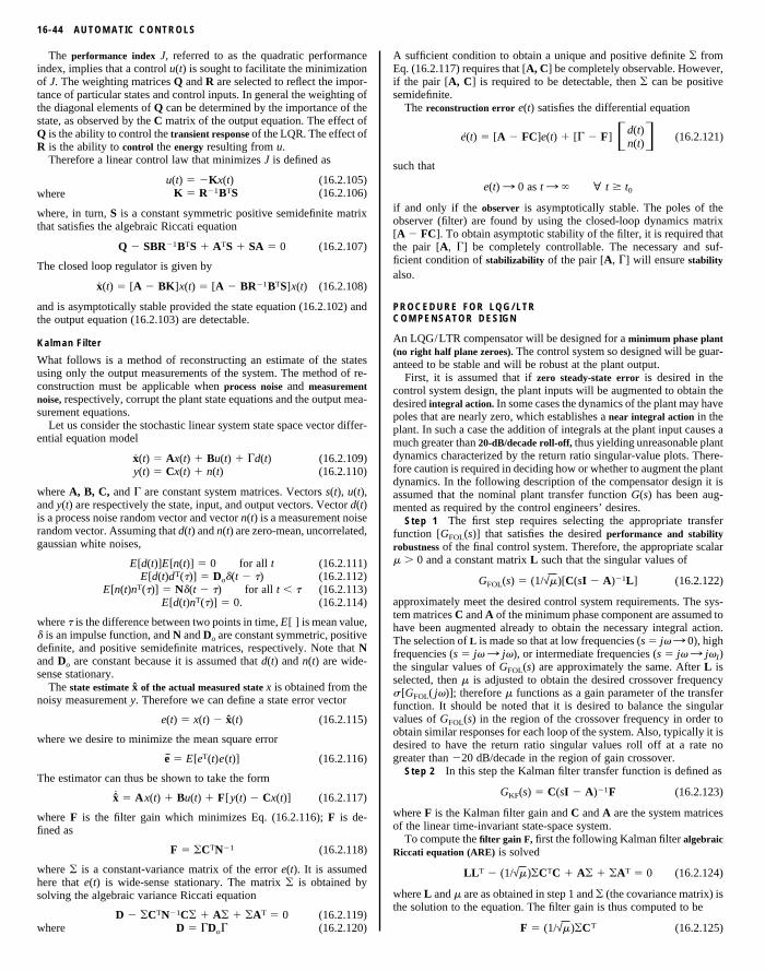
16-44 AUTOMATIC CONTROLS
The performance index J, referred to as the quadratic performanceindex, implies that a control u(t) is sought to facilitate the minimizationof J. The weighting matrices Q and R are selected to reflect the impor-tance of particular states and control inputs. In general the weighting ofthe diagonal elements of Q can be determined by the importance of thestate, as observed by the C matrix of the output equation. The effect ofQ is the ability to control the transient response of the LQR. The effect ofR is the ability to control the energy resulting from u.
Therefore a linear control law that minimizes J is defined as
A sufficient condition to obtain a unique and positive definite o fromEq. (16.2.117) requires that [A, C] be completely observable. However,if the pair [A, C] is required to be detectable, then o can be positivesemidefinite.
The reconstruction error e(t) satisfies the differential equation
~e(t) 5 [A 2 FC]e(t) 1 [G 2 F] Fd(t)n(t)G (16.2.121)
such that
u(t) 5 2Kx(t) (16.2.105)K 5 R21BTS (16.2.106)where
where, in turn, S is a constant symmetric positive semidefinite matrixthat satisfies the algebraic Riccati equation
Q 2 SBR21BTS 1 ATS 1 SA 5 0 (16.2.107)
The closed loop regulator is given by
~x(t) 5 [A 2 BK]x(t) 5 [A 2 BR21BTS]x(t) (16.2.108)
and is asymptotically stable provided the state equation (16.2.102) andthe output equation (16.2.103) are detectable.
Kalman Filter
What follows is a method of reconstructing an estimate of the statesusing only the output measurements of the system. The method of re-construction must be applicable when process noise and measurementnoise, respectively, corrupt the plant state equations and the output mea-surement equations.
Let us consider the stochastic linear system state space vector differ-ential equation model
~x(t) 5 Ax(t) 1 Bu(t) 1 Gd(t) (16.2.109)y(t) 5 Cx(t) 1 n(t) (16.2.110)
where A, B, C, and G are constant system matrices. Vectors s(t), u(t),and y(t) are respectively the state, input, and output vectors. Vector d(t)is a process noise random vector and vector n(t) is a measurement noiserandom vector. Assuming that d(t) and n(t) are zero-mean, uncorrelated,gaussian white noises,
E[d(t)]E[n(t)] 5 0 for all t (16.2.111)E[d(t)dT(t)] 5 Dod(t 2 t) (16.2.112)
E[n(t)nT(t)] 5 Nd(t 2 t) for all t , t (16.2.113)E[d(t)nT(t)] 5 0. (16.2.114)
where t is the difference between two points in time, E[ ] is mean value,d is an impulse function, and N and Do are constant symmetric, positivedefinite, and positive semidefinite matrices, respectively. Note that Nand Do are constant because it is assumed that d(t) and n(t) are wide-sense stationary.
The state estimate x of the actual measured state x is obtained from thenoisy measurement y. Therefore we can define a state error vector
e(t) 5 x(t) 2 x(t) (16.2.115)
where we desire to minimize the mean square error
e 5 E[eT(t)e(t)] (16.2.116)
The estimator can thus be shown to take the form
~x 5 Ax(t) 1 Bu(t) 1 F[y(t) 2 Cx(t)] (16.2.117)
where F is the filter gain which minimizes Eq. (16.2.116); F is de-fined as
F 5 oCTN21 (16.2.118)
where o is a constant-variance matrix of the error e(t). It is assumedhere that e(t) is wide-sense stationary. The matrix o is obtained bysolving the algebraic variance Riccati equation
D 2 oCTN21Co 1 Ao 1 oAT 5 0 (16.2.119)where D 5 GDoG (16.2.120)
e(t) : 0 as t : ` ∀ t $ t0
if and only if the observer is asymptotically stable. The poles of theobserver (filter) are found by using the closed-loop dynamics matrix[A 2 FC]. To obtain asymptotic stability of the filter, it is required thatthe pair [A, G] be completely controllable. The necessary and suf-ficient condition of stabilizability of the pair [A, G] will ensure stability
also.
PROCEDURE FOR LQG/LTRCOMPENSATOR DESIGN
An LQG/LTR compensator will be designed for a minimum phase plant(no right half plane zeroes). The control system so designed will be guar-anteed to be stable and will be robust at the plant output.
First, it is assumed that if zero steady-state error is desired in thecontrol system design, the plant inputs will be augmented to obtain thedesired integral action. In some cases the dynamics of the plant may havepoles that are nearly zero, which establishes a near integral action in theplant. In such a case the addition of integrals at the plant input causes amuch greater than 20-dB/decade roll-off, thus yielding unreasonable plantdynamics characterized by the return ratio singular-value plots. There-fore caution is required in deciding how or whether to augment the plantdynamics. In the following description of the compensator design it isassumed that the nominal plant transfer function G(s) has been aug-mented as required by the control engineers’ desires.
Step 1 The first step requires selecting the appropriate transferfunction [GFOL(s)] that satisfies the desired performance and stabilityrobustness of the final control system. Therefore, the appropriate scalarm . 0 and a constant matrix L such that the singular values of
GFOL(s) 5 (1/√m)[C(sI 2 A)21L] (16.2.122)
approximately meet the desired control system requirements. The sys-tem matrices C and A of the minimum phase component are assumed tohave been augmented already to obtain the necessary integral action.The selection of L is made so that at low frequencies (s 5 jv : 0), highfrequencies (s 5 jv : jv), or intermediate frequencies (s 5 jv : jvI)the singular values of GFOL(s) are approximately the same. After L isselected, then m is adjusted to obtain the desired crossover frequencys [GFOL( jv)]; therefore m functions as a gain parameter of the transferfunction. It should be noted that it is desired to balance the singularvalues of GFOL(s) in the region of the crossover frequency in order toobtain similar responses for each loop of the system. Also, typically it isdesired to have the return ratio singular values roll off at a rate nogreater than 220 dB/decade in the region of gain crossover.
Step 2 In this step the Kalman filter transfer function is defined as
GKF(s) 5 C(sI 2 A)21F (16.2.123)
where F is the Kalman filter gain and C and A are the system matricesof the linear time-invariant state-space system.
To compute the filter gain F, first the following Kalman filter algebraicRiccati equation (ARE) is solved
LLT 2 (1/√m)oCTC 1 Ao 1 oAT 5 0 (16.2.124)
where L and m are as obtained in step 1 and o (the covariance matrix) isthe solution to the equation. The filter gain is thus computed to be
F 5 (1/√m)oCT (16.2.125)
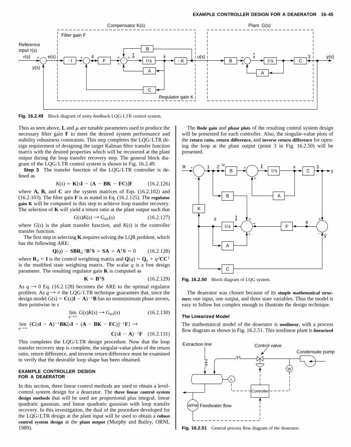
EXAMPLE CONTROLLER DESIGN FOR A DEAERATOR 16-45
r(s) e(s) u(s)
y(s)
y(s)3x4CBF 2K2I I /sI /s
B
A
C
A
Filter gain F
Compensator K(s) Plant G(s)
Regulator gain K
Referenceinput r(s)
1 1 1 1 1
1122
xx
Fig. 16.2.49 Block diagram of unity-feedback LQG/LTR control system.
Thus as seen above, L and m are tunable parameters used to produce thenecessary filter gain F to meet the desired system performance andstability robustness constraints. This step completes the LQG/LTR de-sign requirement of designing the target Kalman filter transfer functionmatrix with the desired properties which will be recovered at the plantoutput during the loop transfer recovery step. The general block dia-gram of the LQG/LTR control system is shown in Fig. 16.2.49.
Step 3 The transfer function of the LQG/LTR controller is de-fined as
The Bode gain and phase plots of the resulting control system designwill be presented for each controller. Also, the singular-value plots ofthe return ratio, return difference, and inverse return difference for open-ing the loop at the plant output (point 3 in Fig. 16.2.50) will bepresented.
RB C yI/s
1 2 3xxu1 1
12
Copyright (C) 1999 by The McGraw-Hill Companies, Inc. All rights reserved. Use ofthis product is subject to the terms of its License Agreement. Click here to view.
K(s) 5 K[sI 2 (A 2 BK 2 FC)]F (16.2.126)
where A, B, and C are the system matrices of Eqs. (16.2.102) and(16.2.103). The filter gain F is as stated in Eq. (16.2.125). The regulatorgain K will be computed in this step to achieve loop transfer recovery.The selection of K will yield a return ratio at the plant output such that
G(s)K(s) : GKF(s) (16.2.127)
where G(s) is the plant transfer function, and K(s) is the controllertransfer function.
The first step in selecting K requires solving the LQR problem, whichhas the following ARE:
Q(q) 2 SBR021BTS 1 SA 1 ATS 5 0 (16.2.128)
where R0 5 I is the control weighting matrix and Q(q) 5 Q0 1 q2CCT
is the modified state weighting matrix. The scalar q is a free designparameter. The resulting regulator gain K is computed as
K 5 BTS (16.2.129)
As q : 0 Eq. (16.2.128) becomes the ARE to the optimal regulatorproblem. As q : ` the LQG/LTR technique guarantees that, since thedesign model G(s) 5 C(s)I 2 A)21B has no nonminimum phase zeroes,then pointwise in s
limq:`
G(s)K(s) : GKF(s) (16.2.130)
limq:`
{C(sI 2 A)21BK[sI 2 (A 2 BK 2 FC)]21F} :
C(sI 2 A)21F (16.2.131)
This completes the LQG/LTR design procedure. Now that the looptransfer recovery step is complete, the singular-value plots of the returnratio, return difference, and inverse return difference must be examinedto verify that the desirable loop shape has been obtained.
EXAMPLE CONTROLLER DESIGNFOR A DEAERATOR
In this section, three linear control methods are used to obtain a level-control system design for a deaerator. The three linear control systemdesign methods that will be used are proportional plus integral, linearquadratic gaussian, and linear quadratic gaussian with loop transferrecovery. In this investigation, the dual of the procedure developed forthe LQG/LTR design at the plant input will be used to obtain a robustcontrol system design at the plant output (Murphy and Bailey, ORNL1989).
A
A
B
K
C
FI/s4
1 11
1 2
x
y
x
Fig. 16.2.50 Block diagram of LQG system.
The deaerator was chosen because of its simple mathematical struc-ture; one input, one output, and three state variables. Thus the model iseasy to follow but complex enough to illustrate the design technique.
The Linearized Model
The mathematical model of the deaerator is nonlinear, with a processflow diagram as shown in Fig. 16.2.51. This nonlinear plant is linearized
Control valve
Feedwater flowWFW
L
W
Controller
Condensate pump
Extraction line
Fig. 16.2.51 General process flow diagram of the deaerator.
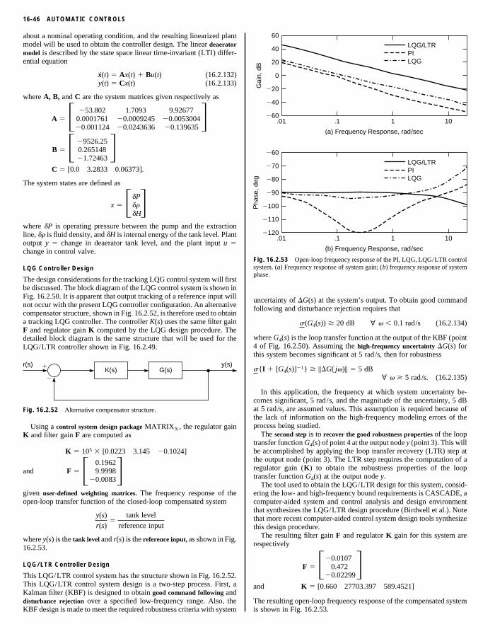
16-46 AUTOMATIC CONTROLS
about a nominal operating condition, and the resulting linearized plantmodel will be used to obtain the controller design. The linear deaeratormodel is described by the state space linear time-invariant (LTI) differ-ential equation
~x(t) 5 Ax(t) 1 Bu(t) (16.2.132)y(t) 5 Cx(t) (16.2.133)
where A, B, and C are the system matrices given respectively as
253.802 1.7093 9.92677
Gai
n, d
B
260
240
220
0
20
40
60
LQG/LTRPILQG
A 5F 0.0001761 20.0009245 20.0053004G20.001124 20.0243636 20.139635
29526.25B 5F 0.265148 G
21.72463
C 5 [0.0 3.2833 0.06373].
The system states are defined as
dPx 5FdrG
dH
where dP is operating pressure between the pump and the extractionline, dr is fluid density, and dH is internal energy of the tank level. Plantoutput y 5 change in deaerator tank level, and the plant input u 5change in control valve.
LQG Controller Design
The design considerations for the tracking LQG control system will firstbe discussed. The block diagram of the LQG control system is shown inFig. 16.2.50. It is apparent that output tracking of a reference input willnot occur with the present LQG controller configuration. An alternativecompensator structure, shown in Fig. 16.2.52, is therefore used to obtaina tracking LQG controller. The controller K(s) uses the same filter gainF and regulator gain K computed by the LQG design procedure. Thedetailed block diagram is the same structure that will be used for theLQG/LTR controller shown in Fig. 16.2.49.
r(s) y(s)G(s)K(s)1
2
Fig. 16.2.52 Alternative compensator structure.
Using a control system design package MATRIXX , the regulator gainK and filter gain F are computed as
K 5 105 3 [0.0223 3.145 20.1024]
0.1962F 5F 9.9998G
20.0083and
given user-defined weighting matrices. The frequency response of theopen-loop transfer function of the closed-loop compensated system
y(s)
r(s)5
tank level
reference input
where y(s) is the tank level and r(s) is the reference input, as shown in Fig.16.2.53.
LQG/LTR Controller Design
This LQG/LTR control system has the structure shown in Fig. 16.2.52.This LQG/LTR control system design is a two-step process. First, aKalman filter (KBF) is designed to obtain good command following anddisturbance rejection over a specified low-frequency range. Also, theKBF design is made to meet the required robustness criteria with system
Pha
se, d
eg
2120
2110
2100
290
280
270
260
LQG/LTRPILQG
(b) Frequency Response, rad/sec
10.01 .1 1
(a) Frequency Response, rad/sec
10.01 .1 1
Fig. 16.2.53 Open-loop frequency response of the PI, LQG, LQG/LTR controlsystem. (a) Frequency response of system gain; (b) frequency response of systemphase.
uncertainty of DG(s) at the system’s output. To obtain good commandfollowing and disturbance rejection requires that
s (G4(s)) $ 20 dB ∀ v , 0.1 rad/s (16.2.134)
where G4(s) is the loop transfer function at the output of the KBF (point4 of Fig. 16.2.50). Assuming the high-frequency uncertainty DG(s) forthis system becomes significant at 5 rad/s, then for robustness
s{I 1 [G4(s)]21} $ ||DG( jv)|| 5 5 dB∀ v $ 5 rad/s. (16.2.135)
In this application, the frequency at which system uncertainty be-comes significant, 5 rad/s, and the magnitude of the uncertainty, 5 dBat 5 rad/s, are assumed values. This assumption is required because ofthe lack of information on the high-frequency modeling errors of theprocess being studied.
The second step is to recover the good robustness properties of the looptransfer function G4(s) of point 4 at the output node y (point 3). This willbe accomplished by applying the loop transfer recovery (LTR) step atthe output node (point 3). The LTR step requires the computation of aregulator gain (K) to obtain the robustness properties of the looptransfer function G4(s) at the output node y.
The tool used to obtain the LQG/LTR design for this system, consid-ering the low- and high-frequency bound requirements is CASCADE, acomputer-aided system and control analysis and design environmentthat synthesizes the LQG/LTR design procedure (Birdwell et al.). Notethat more recent computer-aided control system design tools synthesizethis design procedure.
The resulting filter gain F and regulator K gain for this system arerespectively
20.0107F 5F 0.472 G
20.02299
K 5 [0.660 27703.397 589.4521]and
The resulting open-loop frequency response of the compensated systemis shown in Fig. 16.2.53.
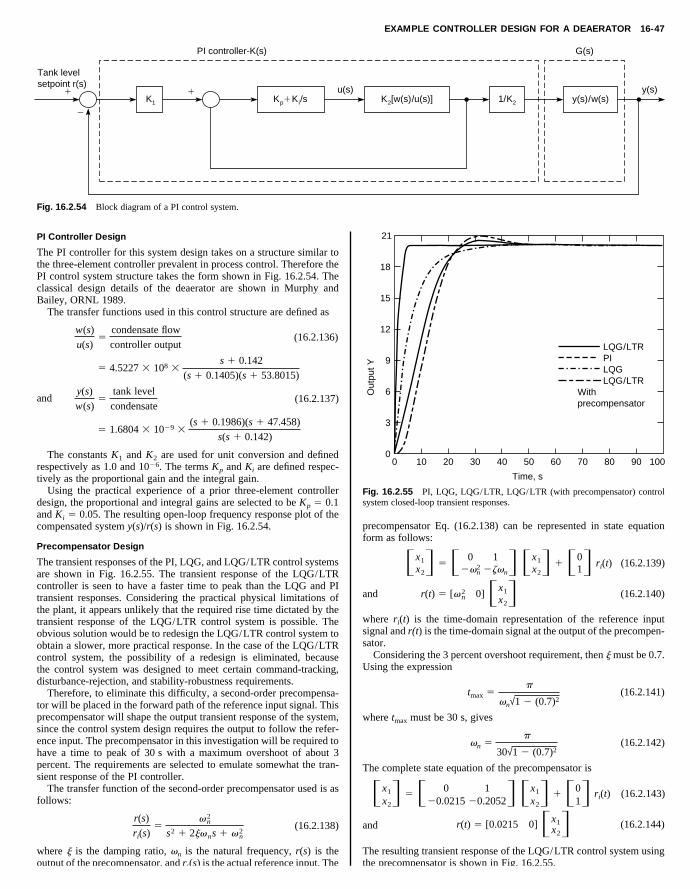
EXAMPLE CONTROLLER DESIGN FOR A DEAERATOR 16-47
y(s)
G(s)PI controller-K(s)
Tank levelsetpoint r(s)
u(s)11
1
2
K1 1/K2Kp K2[w(s)/u(s)] y(s)/w(s)Ki/s
Fig. 16.2.54 Block diagram of a PI control system.
PI Controller Design
The PI controller for this system design takes on a structure similar tothe three-element controller prevalent in process control. Therefore thePI control system structure takes the form shown in Fig. 16.2.54. Theclassical design details of the deaerator are shown in Murphy andBailey, ORNL 1989.
The transfer functions used in this control structure are defined as
w(s)
u(s)5
condensate flow
controller output(16.2.136)
12
15
18
21
LQG/LTR
Copyright (C) 1999 by The McGraw-Hill Companies, Inc. All rights reserved. Use ofthis product is subject to the terms of its License Agreement. Click here to view.
5 4.5227 3 108 3s 1 0.142
(s 1 0.1405)(s 1 53.8015)
y(s)
w(s)5
tank level
condensate(16.2.137)and
5 1.6804 3 1029 3(s 1 0.1986)(s 1 47.458)
s(s 1 0.142)
The constants K1 and K2 are used for unit conversion and definedrespectively as 1.0 and 1026. The terms Kp and Ki are defined respec-tively as the proportional gain and the integral gain.
Using the practical experience of a prior three-element controllerdesign, the proportional and integral gains are selected to be Kp 5 0.1and Ki 5 0.05. The resulting open-loop frequency response plot of thecompensated system y(s)/r(s) is shown in Fig. 16.2.54.
Precompensator Design
The transient responses of the PI, LQG, and LQG/LTR control systemsare shown in Fig. 16.2.55. The transient response of the LQG/LTRcontroller is seen to have a faster time to peak than the LQG and PItransient responses. Considering the practical physical limitations ofthe plant, it appears unlikely that the required rise time dictated by thetransient response of the LQG/LTR control system is possible. Theobvious solution would be to redesign the LQG/LTR control system toobtain a slower, more practical response. In the case of the LQG/LTRcontrol system, the possibility of a redesign is eliminated, becausethe control system was designed to meet certain command-tracking,disturbance-rejection, and stability-robustness requirements.
Therefore, to eliminate this difficulty, a second-order precompensa-tor will be placed in the forward path of the reference input signal. Thisprecompensator will shape the output transient response of the system,since the control system design requires the output to follow the refer-ence input. The precompensator in this investigation will be required tohave a time to peak of 30 s with a maximum overshoot of about 3percent. The requirements are selected to emulate somewhat the tran-sient response of the PI controller.
The transfer function of the second-order precompensator used is asfollows:
r(s)
ri(s)5
vn2
s2 1 2jvns 1 vn2
(16.2.138)
where j is the damping ratio, vn is the natural frequency, r(s) is theoutput of the precompensator, and ri(s) is the actual reference input. The
Out
put Y
0
3
6
9
1009080706050403020100
Time, s
PILQGLQG/LTR
Withprecompensator
Fig. 16.2.55 PI, LQG, LQG/LTR, LQG/LTR (with precompensator) controlsystem closed-loop transient responses.
precompensator Eq. (16.2.138) can be represented in state equationform as follows:
Fx1
x2G 5F 0
2v2n
12zvn
G Fx1
x2G 1F0
1G ri(t) (16.2.139)
and r(t) 5 [v2n 0]Fx1
x2G (16.2.140)
where ri(t) is the time-domain representation of the reference inputsignal and r(t) is the time-domain signal at the output of the precompen-sator.
Considering the 3 percent overshoot requirement, then j must be 0.7.Using the expression
tmax 5p
vn√1 2 (0.7)2(16.2.141)
where tmax must be 30 s, gives
vn 5p
30√1 2 (0.7)2(16.2.142)
The complete state equation of the precompensator is
Fx1
x2G 5F 0
20.02151
20.2052GFx1
x2G 1F0
1G ri(t) (16.2.143)
r(t) 5 [0.0215 0]Fx1x2G (16.2.144)and
The resulting transient response of the LQG/LTR control system usingthe precompensator is shown in Fig. 16.2.55.
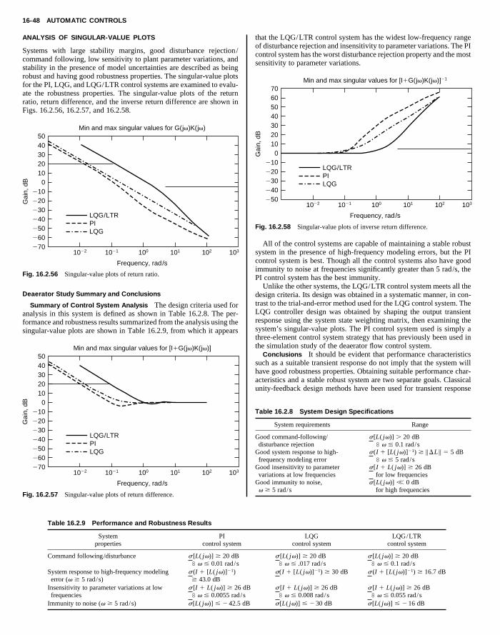
16-48 AUTOMATIC CONTROLS
ANALYSIS OF SINGULAR-VALUE PLOTS
Systems with large stability margins, good disturbance rejection/command following, low sensitivity to plant parameter variations, andstability in the presence of model uncertainties are described as beingrobust and having good robustness properties. The singular-value plotsfor the PI, LQG, and LQG/LTR control systems are examined to evalu-ate the robustness properties. The singular-value plots of the returnratio, return difference, and the inverse return difference are shown inFigs. 16.2.56, 16.2.57, and 16.2.58.
that the LQG/LTR control system has the widest low-frequency rangeof disturbance rejection and insensitivity to parameter variations. The PIcontrol system has the worst disturbance rejection property and the mostsensitivity to parameter variations.
40506070
Min and max singular values for [I1G(jv)K(jv)]21
B
Copyright (C) 1999 by The McGraw-Hill Companies, Inc. All rights reserved. Use ofthis product is subject to the terms of its License Agreement. Click here to view.
Gai
n, d
B
260270
250240230220210
01020304050
1022 1021 100 101 102 103
Frequency, rad/s
Min and max singular values for G(jv)K(jv)
LQG/LTRPILQG
Fig. 16.2.56 Singular-value plots of return ratio.
Deaerator Study Summary and Conclusions
Summary of Control System Analysis The design criteria used foranalysis in this system is defined as shown in Table 16.2.8. The per-formance and robustness results summarized from the analysis using thesingular-value plots are shown in Table 16.2.9, from which it appears
Gai
n, d
B
260270
250240230220210
01020304050
1022 1021 100 101 102 103
Frequency, rad/s
Min and max singular values for [I1G(jv)K(jv)]
LQG/LTRPILQG
Fig. 16.2.57 Singular-value plots of return difference.
Table 16.2.9 Performance and Robustness Results
System PIproperties control system
Command following/disturbance s [L( jv)] $ 20 dB8 v # 0.01 rad/s
System response to high-frequency modelingerror (v $ 5 rad/s)
s (I 1 [L( jv)]21)$ 43.0 dB
Insensitivity to parameter variations at low s [I 1 L( jv)] $ 26 d
frequencies 8 v # 0.0055 rad/sImmunity to noise (v $ 5 rad/s) s[L( jv)] # 2 42.5 dB
Gai
n, d
B
240250
230220210
0102030
1022 1021 100 101 102 103
Frequency, rad/s
LQG/LTRPILQG
Fig. 16.2.58 Singular-value plots of inverse return difference.
All of the control systems are capable of maintaining a stable robustsystem in the presence of high-frequency modeling errors, but the PIcontrol system is best. Though all the control systems also have goodimmunity to noise at frequencies significantly greater than 5 rad/s, thePI control system has the best immunity.
Unlike the other systems, the LQG/LTR control system meets all thedesign criteria. Its design was obtained in a systematic manner, in con-trast to the trial-and-error method used for the LQG control system. TheLQG controller design was obtained by shaping the output transientresponse using the system state weighting matrix, then examining thesystem’s singular-value plots. The PI control system used is simply athree-element control system strategy that has previously been used inthe simulation study of the deaerator flow control system.
Conclusions It should be evident that performance characteristicssuch as a suitable transient response do not imply that the system willhave good robustness properties. Obtaining suitable performance char-acteristics and a stable robust system are two separate goals. Classicalunity-feedback design methods have been used for transient response
Table 16.2.8 System Design Specifications
System requirements Range
Good command-following/disturbance rejection
s[L( jv)] . 20 dB8 v # 0.1 rad/s
Good system response to high-frequency modeling error
s(I 1 [L( jv)]21) $ ||DL || 5 5 dB8 v # 5 rad/s
Good insensitivity to parametervariations at low frequencies
s[I 1 L( jv)] $ 26 dBfor low frequencies
Good immunity to noise,v $ 5 rad/s
s[L( jv)] ,, 0 dBfor high frequencies
LQG LQG/LTRcontrol system control system
s [L( jv)] $ 20 dB8 v # .017 rad/s
s [L( jv)] $ 20 dB8 v # 0.1 rad/s
s(I 1 [L( jv)]21) $ 30 dB s (I 1 [L( jv)]21) $ 16.7 dB
s [I 1 L( jv)] $ 26 dB s [I 1 L( jv)] $ 26 dB
8 v # 0.008 rad/s 8 v # 0.055 rad/ss[L( jv)] # 2 30 dB s[L( jv)] # 2 16 dB
TECHNOLOGY REVIEW 16-49
shaping, with little consideration for robustness properties. The mainadvantage of a closed-loop feedback system is that good performanceand stability robustness properties are obtainable. As has been shown,transient response shaping can be obtained easily using a precompensa-tor. Therefore it appears that the goal of the control system designer isfirst to design a stable robust system and then use prefiltering to obtainthe desired transient response.
Optimal control methods as demonstrated by the LQG control systemdo not guarantee good robustness properties when applied systemati-cally to meet minimization requirements of a performance index. Meth-
troller structure (Wang and Birdwell), which utilizes a fuzzy rule baseto generate gains for a PID controller. Other similar approaches havebeen reported in the literature. An advantage of this approach is theability to establish theoretical results on closed loop stability, which areotherwise lacking for fuzzy controllers.
Signal Validation Technology
Continuous monitoring of instrument channels in a process industryfacility serves many purposes during plant operation. In order toachieve the desired operating condition, the system states must be mea-
Copyright (C) 1999 by The McGraw-Hill Companies, Inc. All rights reserved. Use ofthis product is subject to the terms of its License Agreement. Click here to view.
ods such as pole placement emphasize transient response characteristicswithout regard to robustness, which could be detrimental to the systemintegrity in the presence of model uncertainties.
TECHNOLOGY REVIEW
Fuzzy Control
Fuzzy controllers are a popular method for construction of simple con-trol systems from intuitive knowledge of a process. They generally takethe form of a set of IF . . . THEN . . . rules, where the conditionalparts of the rules have the structure ‘‘Variable i is ,fuzzy value 1.AND Variable j is ,fuzzy value 2. . . . .’’ Here the ,fuzzy value.refers to a membership function, which defines a range of values in whichthe variable may lie and a number between zero and one for each ele-ment of that range specifying the possibility (where certainty is one)that the variable takes that value. Most fuzzy control applications use anerror signal and the rate of change of an error signal as the two variablesto be tested in the conditionals.
The actions of the rules, specified after THEN, take a similar form.Because only a finite collection of membership functions is used, theycan be named by mnemonics which convey meaning to the designer.For example, a fuzzy controller’s rule base might contain the followingrules:
IF temperature-error is high and temperature-error-rate is slowTHEN fuel-rate is negative.
IF temperature-error is zero and temperature-error-rate is slowTHEN fuel-rate is zero.
Fuzzy controllers are an attractive control design approach because ofthe ease with which fuzzy rules can be interpreted and can be made tofollow a designer’s intuitive knowledge regarding the control structure.They are inherently nonlinear, so it is easy to incorporate effects whichmimic variable gains by adjusting either the rules or the definitions ofthe membership functions. Fuzzy controller technology is attractive, inpart because of its intuitive appeal and its nonlinear nature, but alsobecause of the frequent claim that fuzzy rules can be utilized to approxi-mate arbitrary continuous functional relationships. While this is true, infact it would require substantial complexity to construct a fuzzy rulebase to mimic a desired function sufficiently well for most engineers tolabel it an approximation. Herein also lie the potential liabilities offuzzy controller technology: there is very little theoretical guidance onhow rules and membership functions should be specified. Fuzzy con-troller design is an intuitive process; if intuition fails the designer, one isleft with very little beyond trial and error.
One remedy for this situation is the use of machine, or automatedlearning technology to infer fuzzy controller rules from either collecteddata or simulation of a process model. This process is inference, ratherthan deductive reasoning, in that proper operation of the controller islearning by example, so if the examples do not adequately describe theprocess, problems can occur. This inference process, however, is quitesimilar to the methods of system identification, which also infer modelstructure from examples, and which is an accepted method of modelconstruction. Machine learning technology enables utilization of morecomplex controller structures as well, which introduce additional de-grees of freedom in the design process but also enhance the capabilitiesof the controller. One example of this approach is the Fuzzy PID con-
sured accurately. This may be accomplished by implementing a reliablesignal validation procedure during both normal and transient operations.Such a system would help reduce challenges on control systems, mini-mize plant downtime, and help plan maintenance tasks. Examples ofmeasurements include pressure, temperature, flow, liquid level, electri-cal parameters, machinery vibration, and many others. The performanceof control, safety, and plant monitoring systems depends on the accu-racy of signals being used in these systems. Signal validation is definedas the detection, isolation, and characterization of faulty signals. Thistechnique must be applicable to systems with redundant or single sensorconfiguration.
Various methods have been developed for signal validation in aero-space, power, chemical, metals, and other process industries. Most ofthe early development was in the aerospace industry. The signal valida-tion techniques vary in complexity depending on the level of informa-tion to be extracted. Both model-based and direct data-based techniquesare now available. The following is a list of techniques often imple-mented for signal validation:
Consistency checking of redundant sensorsSequential probability ratio testing for incipient fault detectionProcess empirical modeling (static and dynamic) for state estimationComputational neural networks for state estimationKalman filtering technique for state estimation in both linear and
nonlinear systemsTime-series modeling techniques for sensor response time estimation
and frequency bandwidth monitoring
PC-based signal validation systems (Upadhyaya, 1989) are now avail-able and are being implemented on-line in various industries. The com-puter software system consists of one or more of the above signal pro-cessing modules, with a decision maker that provides sensor statusinformation to the operator.
An example of signal validation (Upadhyaya and Eryurek) in a powerplant is the monitoring of water level in a steam generator. The objec-tive is to estimate the water level using other related measurements andcompare this with the measured level. An empirical model, a neuralnetwork model, or the Kalman filtering technique may be used. Forexample, the inputs to an empirical model consist of steam generatormain feedwater flow rate, steam generator pressure, and inlet and outlettemperatures of the primary water through the steam generator. Such amodel would be developed during normal plant operation, and is gener-ally referred to as the training phase. The signal estimation modelsshould be updated according to the plant operational status. The use ofmultiple signal validation modules provides a high degree of confidencein the results.
Chaos
Recent advances in dynamical process analysis have revealed that non-linear interactions in simple deterministic processes can often result inhighly complex, aperiodic, sometimes apparently ‘‘random’’ behavior.Processes which exhibit such behavior are said to be exhibit determinis-tic chaos. The term chaos is perhaps unfortunate for describing thisbehavior. It evokes images of purely erratic behavior, but this phenom-enon actually involves highly structured patterns. It is now recognizedthat deterministic chaos dominates many engineering systems of practi-cal interest, and that, in many cases, it may be possible to exploit previ-ously unrecognized deterministic structure for improved understandingand control.
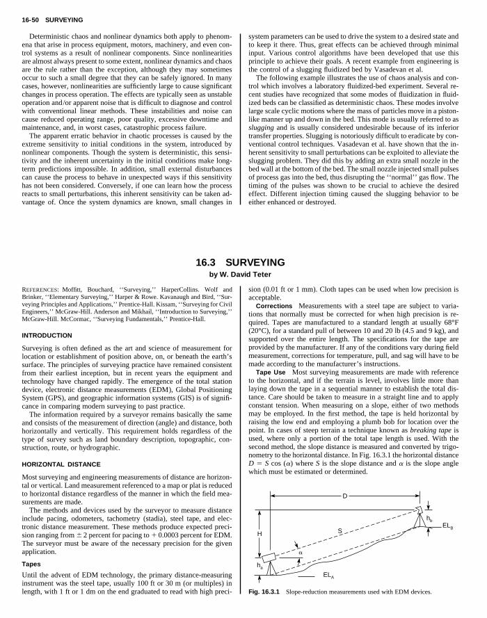
16-50 SURVEYING
Deterministic chaos and nonlinear dynamics both apply to phenom-ena that arise in process equipment, motors, machinery, and even con-trol systems as a result of nonlinear components. Since nonlinearitiesare almost always present to some extent, nonlinear dynamics and chaosare the rule rather than the exception, although they may sometimesoccur to such a small degree that they can be safely ignored. In manycases, however, nonlinearities are sufficiently large to cause significantchanges in process operation. The effects are typically seen as unstableoperation and/or apparent noise that is difficult to diagnose and controlwith conventional linear methods. These instabilities and noise can
system parameters can be used to drive the system to a desired state andto keep it there. Thus, great effects can be achieved through minimalinput. Various control algorithms have been developed that use thisprinciple to achieve their goals. A recent example from engineering isthe control of a slugging fluidized bed by Vasadevan et al.
The following example illustrates the use of chaos analysis and con-trol which involves a laboratory fluidized-bed experiment. Several re-cent studies have recognized that some modes of fluidization in fluid-ized beds can be classified as deterministic chaos. These modes involvelarge scale cyclic motions where the mass of particles move in a piston-
Rav
Copyright (C) 1999 by The McGraw-Hill Companies, Inc. All rights reserved. Use ofthis product is subject to the terms of its License Agreement. Click here to view.
cause reduced operating range, poor quality, excessive downtime andmaintenance, and, in worst cases, catastrophic process failure.
The apparent erratic behavior in chaotic processes is caused by theextreme sensitivity to initial conditions in the system, introduced bynonlinear components. Though the system is deterministic, this sensi-tivity and the inherent uncertainty in the initial conditions make long-term predictions impossible. In addition, small external disturbancescan cause the process to behave in unexpected ways if this sensitivityhas not been considered. Conversely, if one can learn how the processreacts to small perturbations, this inherent sensitivity can be taken ad-vantage of. Once the system dynamics are known, small changes in
16.3 SUby W. D
REFERENCES: Moffitt, Bouchard, ‘‘Surveying,’’ HarperCollins. Wolf and
Brinker, ‘‘Elementary Surveying,’’ Harper & Rowe. Kavanaugh and Bird, ‘‘Sur-veying Principles and Applications,’’ Prentice-Hall. Kissam, ‘‘Surveying for CivilEngineers,’’ McGraw-Hill. Anderson and Mikhail, ‘‘Introduction to Surveying,’’McGraw-Hill. McCormac, ‘‘Surveying Fundamentals,’’ Prentice-Hall.INTRODUCTION
Surveying is often defined as the art and science of melocation or establishment of position above, on, or benea
like manner up and down in the bed. This mode is usually referred to asslugging and is usually considered undesirable because of its inferiortransfer properties. Slugging is notoriously difficult to eradicate by con-ventional control techniques. Vasadevan et al. have shown that the in-herent sensitivity to small perturbations can be exploited to alleviate theslugging problem. They did this by adding an extra small nozzle in thebed wall at the bottom of the bed. The small nozzle injected small pulsesof process gas into the bed, thus disrupting the ‘‘normal’’ gas flow. Thetiming of the pulses was shown to be crucial to achieve the desiredeffect. Different injection timing caused the slugging behavior to beeither enhanced or destroyed.
VEYINGid Teter
sion (0.01 ft or 1 mm). Cloth tapes can be used when low precision is
acceptable.Corrections Measurements with a steel tape are subject to varia-tions that normally must be corrected for when high precision is re-quired. Tapes are manufactured to a standard length at usually 68°F(20°C), for a standard pull of between 10 and 20 lb (4.5 and 9 kg), and
the entire length. The specifications for the tape areanufacturer. If any of the conditions vary during field
rrections for temperature, pull, and sag will have to be
asurement forth the earth’ssupported overprovided by the mmeasurement, co
made according to the manufacturer’s instructions. surface. The principles of surveying practice have remained consistentfrom their earliest inception, but in recent years the equipment andtechnology have changed rapidly. The emergence of the total stationdevice, electronic distance measurements (EDM), Global PositioningSystem (GPS), and geographic information systems (GIS) is of signifi-cance in comparing modern surveying to past practice.
The information required by a surveyor remains basically the sameand consists of the measurement of direction (angle) and distance, bothhorizontally and vertically. This requirement holds regardless of thetype of survey such as land boundary description, topographic, con-struction, route, or hydrographic.
HORIZONTAL DISTANCE
Most surveying and engineering measurements of distance are horizon-tal or vertical. Land measurement referenced to a map or plat is reducedto horizontal distance regardless of the manner in which the field mea-surements are made.
The methods and devices used by the surveyor to measure distanceinclude pacing, odometers, tachometry (stadia), steel tape, and elec-tronic distance measurement. These methods produce expected preci-sion ranging from 6 2 percent for pacing to 1 0.0003 percent for EDM.The surveyor must be aware of the necessary precision for the givenapplication.
Tapes
Until the advent of EDM technology, the primary distance-measuringinstrument was the steel tape, usually 100 ft or 30 m (or multiples) inlength, with 1 ft or 1 dm on the end graduated to read with high preci-
Tape Use Most surveying measurements are made with referenceto the horizontal, and if the terrain is level, involves little more thanlaying down the tape in a sequential manner to establish the total dis-tance. Care should be taken to measure in a straight line and to applyconstant tension. When measuring on a slope, either of two methodsmay be employed. In the first method, the tape is held horizontal byraising the low end and employing a plumb bob for location over thepoint. In cases of steep terrain a technique known as breaking tape isused, where only a portion of the total tape length is used. With thesecond method, the slope distance is measured and converted by trigo-nometry to the horizontal distance. In Fig. 16.3.1 the horizontal distanceD 5 S cos (a) where S is the slope distance and a is the slope anglewhich must be estimated or determined.
D
H
ELA
ELB
hb
ha
S
a
Fig. 16.3.1 Slope-reduction measurements used with EDM devices.
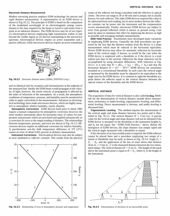
VERTICAL DISTANCE 16-51
Electronic Distance Measurement
Modern surveying practice employs EDM technology for precise andrapid distance measurement. A representation of an EDM device isshown in Fig 16.3.2. The principle of EDM is based on the comparisonof the modulated wavelength of an electromagnetic energy source(beam) to the time required for the beam to travel to and return from apoint at an unknown distance. The EDM devices may be of two types:(1) electrooptical devices employing light transmission within or justbeyond the visible region or (2) devices transmitting in the microwave
center of the reflector not being coincident with the effective or opticalcenter. The error can range to 30 or 40 mm and is unique, but is usuallyknown, for each reflector. The older EDM devices required this value tobe subtracted from each reading, but in more modern devices the reflec-tor constant can be preset into the instrument and the compensationoccurs automatically. Finally, microwave EDM devices are subject toerror from ground reflection which is known as ground swing. Caremust be taken to minimize this effect by deploying the devices as highas possible and averaging multiple measurements.
EDM Field Practice Practitioners have developed many variations
Copyright (C) 1999 by The McGraw-Hill Companies, Inc. All rights reserved. Use ofthis product is subject to the terms of its License Agreement. Click here to view.
spectrum. Electrooptical devices require an active transmitter and apassive reflector, while microwave devices require an active transmitter
Fig. 16.3.2 Electronic distance meter (EDM). (PENTAX Corp.)
and an identical unit for reception and retransmission at the endpoint ofthe measured line. Ideally the EDM beam would propagate at the veloc-ity of light; however, the actual velocity of propagation is affected bythe index of refraction of the atmosphere. As a result, the atmosphericconditions of temperature, pressure, and humidity must be monitored inorder to apply corrections to the measurements. Advances in electroop-tical technology have made microwave devices, which are highly sensi-tive to atmospheric relative humidity, nearly obsolete.
Atmospheric Corrections EDM devices built prior to about 1982require a manual computation for atmospheric correction; however, themore modern instruments allow for keystroke entry of values for tem-perature and pressure which are processed and applied automatically asa correction for error to the output reading of distance. The relationshipsbetween temperature, pressure, and error are shown in Fig. 16.3.3. Mi-crowave devices require an additional correction for relative humidity.A psychrometer wet-dry bulb temperature difference of 3°F (2°C)causes an error of about 0.001 percent in distance measurement.
Instrument Corrections Electrooptical devices may also be subjectto error attributed to reflector constant. This results from the physical
T, °
C
25
20
15
10
02.002 2.001 0 .001 .002
P, m
mH
g
Error, %
810
785
760
735
710
T P
TP
Fig. 16.3.3 Relationship of error to atmospheric pressure and temperature.
in employing EDM devices. Generally the field procedures are gov-erned by the fact that the distance readout from the device is a slopemeasurement which must be reduced to the horizontal equivalent.Newer EDM devices may allow for automatic reduction by keystrokeinput of the vertical angle, if known, as would be the case when theEDM device is employed with a theodolite or if the device is a totalstation (see later in the section). Otherwise the slope reduction can beaccomplished by using elevation differences. With reference to Fig.16.3.1, it is seen that H 5 (ELA 1 ha) 2 (ELB 1 hb ) and that thehorizontal distance D 5 (S2 2 H2)1/2. EDM devices are sometimesmounted on a conventional theodolite. In such cases the vertical angleas measured by the theodolite must be adjusted to be equivalent to theangle seen by the EDM device. It is common to sight the theodolite at apoint below the reflector equal to the vertical distance between theoptical centers of the theodolite and the EDM device.
VERTICAL DISTANCE
The acquisition of data for vertical distance is also called leveling. Meth-ods for the determination of vertical distance include direct measure-ment, tachometry or stadia leveling, trigonometric leveling, and differ-ential leveling. Direct measurement is obvious, and stadia leveling isdiscussed later.
Trigonometric Leveling This method requires the measurement ofthe vertical angle and slope distance between two points and is illus-trated in Fig. 16.3.1. The vertical distance H 5 S sin (a). A precisevalue for the vertical angle and slope distance will not be obtained if theEDM device is mounted on the theodolite or the instrument heights ha
and hb are not equal. See ‘‘EDM Field Practice,’’ above. Before theemergence of EDM devices, the slope distance was simply taped andthe vertical angle measured with a theodolite or transit.
If the elevation of an inaccessible point is required, the EDM reflectorcannot be placed there and a procedure employing two setups of atransit or theodolite may be used, as shown in Fig. 16.3.4. Angle Z3 5Z1 2 Z2 , and the application of the law of sines shows that distanceA/sin Z2 5 C/sin Z3 . C is the measured distance between the two instru-ment setups. The vertical distance H 5 A sin Z1 . The height of the stackabove the instrument point is equal to H 1 h1 , where h1 is the height ofthe instrument.
C
AB H
Z2 Z1
Z3
h1
Fig. 16.3.4 Determination of elevation of an inaccessible point.
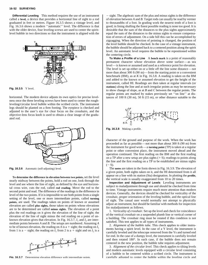
16-52 SURVEYING
Differential Leveling This method requires the use of an instrumentcalled a level, a device that provides a horizontal line of sight to a rodgraduated in feet or metres. Figure 16.3.5 shows a vintage level, andFig. 16.3.6 shows a modern ‘‘automatic’’ level. The difference is thatwith the older device, four leveling screws are used to center the spirit-level bubble in two directions so that the instrument is aligned with the
2 sight. The algebraic sum of the plus and minus sights is the differenceof elevation between A and B. Target rods can usually be read by vernierto thousandths of a foot. In grading work the nearest tenth of a foot isgood; in lining shafting the finest possible reading is none too good. It isdesirable that the sum of the distances to the plus sights approximatelyequal the sum of the distances to the minus sights to ensure compensa-tion of errors of adjustment. On a side hill this can be accomplished byzigzagging. When the direction of pointing is changed, the position ofthe level bubble should be checked. In the case of a vintage instrument,the bubble should be adjusted back to a centered position along the spirit
Copyright (C) 1999 by The McGraw-Hill Companies, Inc. All rights reserved. Use ofthis product is subject to the terms of its License Agreement. Click here to view.
Fig. 16.3.5 Y level.
horizontal. The modern device adjusts its own optics for precise level-ness once the three leveling screws have been used to center the rough-leveling/circular level bubble within the scribed circle. The instrumentlegs should be planted on a firm footing. The eyepiece is checked andadjusted to the user’s eye for clear focus on the crosshairs, and theobjective-lens focus knob is used to obtain a clear image of the gradu-ated rod.
Fig. 16.3.6 Automatic (self-adjusting) level.
To determine the difference in elevation between two points, set the levelnearly midway between the points, hold a rod on one, look through thelevel and see where the line of sight, as defined by the eye and horizon-tal cross wire, cuts the rod, called rod reading. Move the rod to thesecond point and read. The difference of the readings is the difference inlevel of the two points. If it is impossible to see both points from a singlesetting of the level, one or more intermediate points, called turningpoints, are used. The readings taken on points of known or assumedelevation are called plus sights, those taken on points whose elevationsare to be determined are called minus sights. The elevation of a pointplus the rod readings on it gives the elevation of the line of sight; theelevation of the line of sight minus the rod reading on a point of un-known elevation gives that elevation. In Fig. 16.3.7, I1 and I2 are inter-mediate points between A and B. The setups are numbered. Assuming Ato be of known elevation, the reading on A is a 1 sight; the reading on I1
from 1 is a 2 sight; the reading on I1 from 2 is a 1 sight and on I2 is a
Fig. 16.3.7 Determining elevation difference with intermediate points.
level. An automatic level requires the bubble to be repositioned withinthe centering circle.
To Make a Profile of a Line A bench mark is a point of reasonablypermanent character whose elevation above some surface—as sealevel—is known or assumed and used as a reference point for elevation.The level is set up either on or a little off the line some distance—notmore than about 300 ft (90 m)—from the starting point or a convenientbenchmark (BM), as at K in Fig. 16.3.8. A reading is taken on the BMand added to the known or assumed elevation to get the height of theinstrument, called HI. Readings are then taken at regular intervals (orstations) along the line and at such irregular points as may be necessaryto show change of slope, as at B and C between the regular points. Theregular points are marked by stakes previously set ‘‘on line’’ at dis-tances of 100 ft (30 m), 50 ft (15 m), or other distance suitable to the
Fig. 16.3.8 Making a profile.
character of the ground and purpose of the work. When the work hasproceeded as far as possible—not more than about 300 ft (90 m) fromthe instrument for good work—a turning point (TP) is taken at a regularpoint or other convenient place, the instrument moved ahead and theoperation continued. The first reading on the BM and the first readingon a TP after a new setup are plus sights (1 S); readings to points alongthe line and the first reading on a TP to be established are minus sights(2 S).
The notes are taken in the form shown in Fig. 16.3.9. The elevation ofa given point, both sights taken on it, and the HI determined from it allappear on a line with its station (Sta) designation. In plotting the profile,the vertical scale is usually exaggerated from 10 to 20 times.
Inspection and Adjustment of Levels Leveling instruments aresubject to maladjustment through use and should be checked from timeto time. Vintage instruments require much more attention than moderndevices. Generally, the devices should be checked for verticality of thecrosshair, proper orientation of the leveling bubble, and the optical lineof sight. The casual user would normally not attempt to physicallyadjust an instrument, but should be familiar with methods for inspectionfor maladjustment as follows.
1. Verticality of crosshair. Set up the level and check for coincidenceof the vertical crosshair on a suspended plumb line or vertical corner ofa building. The crosshair ring must be rotated if this condition is notsatisfied. This test applies to all types of instruments.
2. Alignment of the bubble tube. This check applies to older instru-ments having a spirit level. In the case of a Y level, the instrument iscarefully leveled and the telescope removed from the Ys and turned endfor end. In the case of a dumpy level, the instrument is carefully leveledand then rotated 180°. In each case, if the bubble does not remaincentered in the new position, the bubble tube requires adjustment.
3. Alignment of the circular level. This check applies to tilting levelsand modern automatic levels equipped with a circular level consistingof a bubble to be centered within a scribed circle. The instrument iscarefully adjusted to center the bubble within the leveling circle and
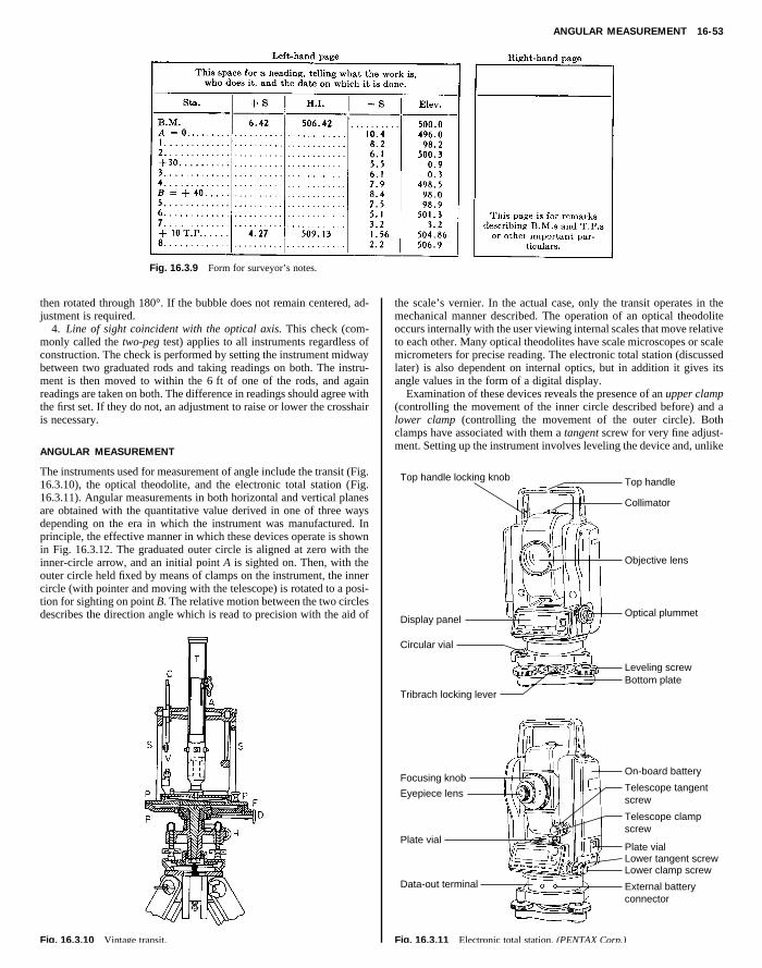
ANGULAR MEASUREMENT 16-53
Fig. 16.3.9 Form for surveyor’s notes.
then rotated through 180°. If the bubble does not remain centered, ad-justment is required.
4. Line of sight coincident with the optical axis. This check (com-monly called the two-peg test) applies to all instruments regardless ofconstruction. The check is performed by setting the instrument midwaybetween two graduated rods and taking readings on both. The instru-ment is then moved to within the 6 ft of one of the rods, and againreadings are taken on both. The difference in readings should agree withthe first set. If they do not, an adjustment to raise or lower the crosshairis necessary.
the scale’s vernier. In the actual case, only the transit operates in themechanical manner described. The operation of an optical theodoliteoccurs internally with the user viewing internal scales that move relativeto each other. Many optical theodolites have scale microscopes or scalemicrometers for precise reading. The electronic total station (discussedlater) is also dependent on internal optics, but in addition it gives itsangle values in the form of a digital display.
Examination of these devices reveals the presence of an upper clamp(controlling the movement of the inner circle described before) and alower clamp (controlling the movement of the outer circle). Both
Copyright (C) 1999 by The McGraw-Hill Companies, Inc. All rights reserved. Use ofthis product is subject to the terms of its License Agreement. Click here to view.
ANGULAR MEASUREMENT
The instruments used for measurement of angle include the transit (Fig.16.3.10), the optical theodolite, and the electronic total station (Fig.16.3.11). Angular measurements in both horizontal and vertical planesare obtained with the quantitative value derived in one of three waysdepending on the era in which the instrument was manufactured. Inprinciple, the effective manner in which these devices operate is shownin Fig. 16.3.12. The graduated outer circle is aligned at zero with theinner-circle arrow, and an initial point A is sighted on. Then, with theouter circle held fixed by means of clamps on the instrument, the innercircle (with pointer and moving with the telescope) is rotated to a posi-tion for sighting on point B. The relative motion between the two circlesdescribes the direction angle which is read to precision with the aid of
Fig. 16.3.10 Vintage transit.
clamps have associated with them a tangent screw for very fine adjust-ment. Setting up the instrument involves leveling the device and, unlike
Top handle locking knob Top handle
Display panel
Focusing knob
Eyepiece lens
Plate vial
Data-out terminal
Circular vial
Tribrach locking lever
Collimator
Telescope tangentscrew
Objective lens
Optical plummet
Leveling screwBottom plate
On-board battery
Plate vial
Telescope clampscrew
Lower clamp screwLower tangent screw
External batteryconnector
Fig. 16.3.11 Electronic total station. (PENTAX Corp.)
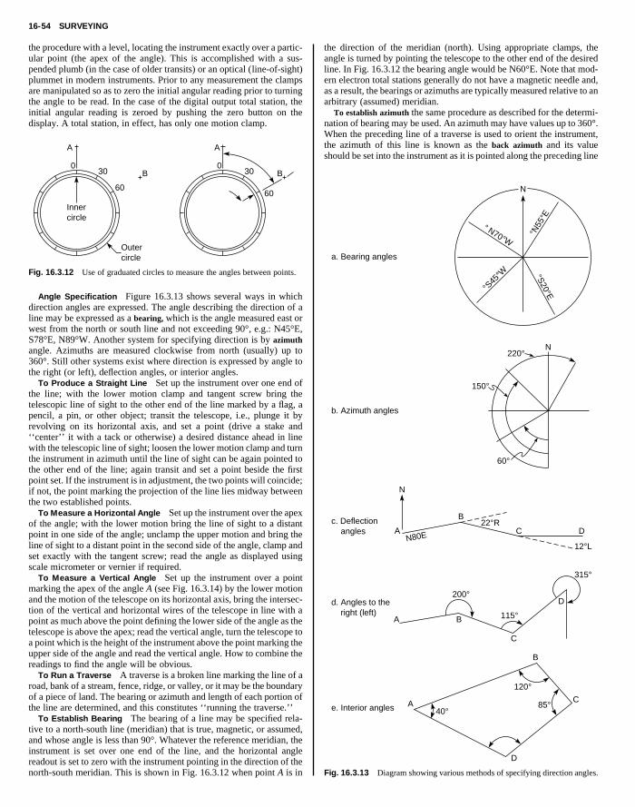
16-54 SURVEYING
the procedure with a level, locating the instrument exactly over a partic-ular point (the apex of the angle). This is accomplished with a sus-pended plumb (in the case of older transits) or an optical (line-of-sight)plummet in modern instruments. Prior to any measurement the clampsare manipulated so as to zero the initial angular reading prior to turningthe angle to be read. In the case of the digital output total station, theinitial angular reading is zeroed by pushing the zero button on thedisplay. A total station, in effect, has only one motion clamp.
A A
the direction of the meridian (north). Using appropriate clamps, theangle is turned by pointing the telescope to the other end of the desiredline. In Fig. 16.3.12 the bearing angle would be N60°E. Note that mod-ern electron total stations generally do not have a magnetic needle and,as a result, the bearings or azimuths are typically measured relative to anarbitrary (assumed) meridian.
To establish azimuth the same procedure as described for the determi-nation of bearing may be used. An azimuth may have values up to 360°.When the preceding line of a traverse is used to orient the instrument,the azimuth of this line is known as the back azimuth and its value
Copyright (C) 1999 by The McGraw-Hill Companies, Inc. All rights reserved. Use ofthis product is subject to the terms of its License Agreement. Click here to view.
B B0
30
60
030
60
Innercircle
Outercircle
Fig. 16.3.12 Use of graduated circles to measure the angles between points.
Angle Specification Figure 16.3.13 shows several ways in whichdirection angles are expressed. The angle describing the direction of aline may be expressed as a bearing, which is the angle measured east orwest from the north or south line and not exceeding 90°, e.g.: N45°E,S78°E, N89°W. Another system for specifying direction is by azimuthangle. Azimuths are measured clockwise from north (usually) up to360°. Still other systems exist where direction is expressed by angle tothe right (or left), deflection angles, or interior angles.
To Produce a Straight Line Set up the instrument over one end ofthe line; with the lower motion clamp and tangent screw bring thetelescopic line of sight to the other end of the line marked by a flag, apencil, a pin, or other object; transit the telescope, i.e., plunge it byrevolving on its horizontal axis, and set a point (drive a stake and‘‘center’’ it with a tack or otherwise) a desired distance ahead in linewith the telescopic line of sight; loosen the lower motion clamp and turnthe instrument in azimuth until the line of sight can be again pointed tothe other end of the line; again transit and set a point beside the firstpoint set. If the instrument is in adjustment, the two points will coincide;if not, the point marking the projection of the line lies midway betweenthe two established points.
To Measure a Horizontal Angle Set up the instrument over the apexof the angle; with the lower motion bring the line of sight to a distantpoint in one side of the angle; unclamp the upper motion and bring theline of sight to a distant point in the second side of the angle, clamp andset exactly with the tangent screw; read the angle as displayed usingscale micrometer or vernier if required.
To Measure a Vertical Angle Set up the instrument over a pointmarking the apex of the angle A (see Fig. 16.3.14) by the lower motionand the motion of the telescope on its horizontal axis, bring the intersec-tion of the vertical and horizontal wires of the telescope in line with apoint as much above the point defining the lower side of the angle as thetelescope is above the apex; read the vertical angle, turn the telescope toa point which is the height of the instrument above the point marking theupper side of the angle and read the vertical angle. How to combine thereadings to find the angle will be obvious.
To Run a Traverse A traverse is a broken line marking the line of aroad, bank of a stream, fence, ridge, or valley, or it may be the boundaryof a piece of land. The bearing or azimuth and length of each portion ofthe line are determined, and this constitutes ‘‘running the traverse.’’
To Establish Bearing The bearing of a line may be specified rela-tive to a north-south line (meridian) that is true, magnetic, or assumed,and whose angle is less than 90°. Whatever the reference meridian, theinstrument is set over one end of the line, and the horizontal anglereadout is set to zero with the instrument pointing in the direction of thenorth-south meridian. This is shown in Fig. 16.3.12 when point A is in
should be set into the instrument as it is pointed along the preceding line
N
N
N
A
B
B
C
C
A
A
B
C
D
D
D
220°
150°
60°
a. Bearing angles
b. Azimuth angles
c. Deflection angles
d. Angles to the right (left)
e. Interior angles
°N55
°E
°S20°E°S
45°W
° N70°W
N80E
22°R
200°
40°85°
120°
115°
315°
12°L
Fig. 16.3.13 Diagram showing various methods of specifying direction angles.
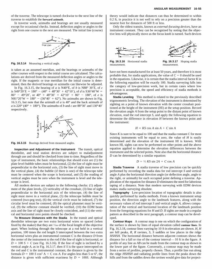
ANGULAR MEASUREMENT 16-55
of the traverse. The telescope is turned clockwise to the next line of thetraverse to establish the forward azimuth.
In traverse work, azimuths and bearings are not usually measuredexcept for occasional checks. Instead, deflection angles or angles to theright from one course to the next are measured. The initial line (course)
theory would indicate that distances can thus be determined to within0.2 ft, in practice it is not well to rely on a precision greater than thenearest foot for distances of 500 ft or less.
Only the oldest transits, known as external-focusing devices, have aninstrument constant. They can be recognized by noting that the objec-tive lens will physically move as the focus knob is turned. Such devices
Copyright (C) 1999 by The McGraw-Hill Companies, Inc. All rights reserved. Use ofthis product is subject to the terms of its License Agreement. Click here to view.
Fig. 16.3.14 Measuring a vertical angle.
is taken as an assumed meridian, and the bearings or azimuths of theother courses with respect to the initial course are calculated. The calcu-lations are derived from the measured deflection angles or angles to theright. If the magnetic or true meridian for the initial course is deter-mined, then the derived bearings or azimuths can likewise be adjusted.
In Fig. 16.3.15, the bearing of a is N40°E, of b is N88° 309E, of cis S49°209E 5 180° 2 (40° 1 48°309 1 42°109), of d is S36°409W 586° 2 49°209, or 40° 1 48°309 1 42°109 1 86° 2 180°, of e isN81°209W 5 180° 2 (36°409 1 62°). No azimuths are shown in Fig.16.3.15, but note that the azimuth of a is 40° and the back azimuth ofa is 220° (40°1 180°). The azimuths of b and c are 88°309 and 130°409respectively.
Fig. 16.3.15 Bearings derived from measured angles.
Inspection and Adjustment of the Instrument The transit, opticaltheodolite, and total station devices are subject to maladjustmentthrough use and should be checked from time to time. Regardless of thetype of instrument, the basic relationships that should exist are (1) theplate level-bubble tubes must be horizontal, (2) the line of sight must beperpendicular to the horizontal axis, (3) the line of sight must move inthe vertical plane, (4) the bubble (if there is one) of the telescope tubemust be centered when the scope is horizontal, and (5) the reading ofvertical angles must be zero when the instrument is level and the tele-scope is level.
All modern devices are subject to the following checks: (1) adjust-ment of the plate levels, (2) verticality of the crosshair, (3) line of sightperpendicular to the horizontal axis of the telescope, (4) the line ofsight must move in a vertical plane, (5) the telescope bubble must becentered (two-peg test), (6) the vertical circle must be indexed, (7) thecircular level must be centered, (8) the optical plummet must be verti-cal, (9) the reflector constant should be verified, (10) the EDM beamaxis and the line of sight must be closely coincident, and (11) the verti-cal and horizontal zero points should be checked.
To Measure Distances with the Stadia In the transit and opticaltheodolite telescope are two extra horizontal wires so spaced (whenfixed by the maker) that they are 1⁄100 of the focal length of the objectiveapart. When looking through the telescope at a rod held in a verticalposition, 100 times the rod length S intercepted between the two extrahorizontal wires plus an instrumental constant C is the distance D fromthe center of the instrument to the rod if the line of sight is horizontal, orD 5 100 S 1 C (see Fig. 16.3.16). If the line of sight is inclined by avertical angle A, as in Fig. 16.3.17, then if S is the space intercepted onthe rod and C is the instrumental constant, the distance is given by theformula D 5 100 S cos2 A 1 C cos A. For angles less than 5 or 6°, thedistance is given with sufficient exactness by D 5 100S. Although
Fig. 16.3.16 Horizontal stadiameasurement.
Fig. 16.3.17 Sloping stadiameasurement.
have not been manufactured for at least 50 years, and therefore it is mostprobable that, for stadia applications, the value of C 5 0 should be usedin the equations. Likewise, it is certain that the stadia interval factor K inthe following equation will be exactly 100. Stadia surveying falls intothe category of low-precision work, but in certain cases where lowprecision is acceptable, the speed and efficiency of stadia methods isadvantageous.
Stadia Leveling This method is related to the previously describedtrigonometric leveling. The elevation of the instrument is determined bysighting on a point of known elevation with the center crosshair posi-tioned at the height of the instrument (HI) at the setup position. Recordthe elevation angle A from the setup point to the distant point of knownelevation, read the rod intercept S, and apply the following equation todetermine the difference in elevation H between the known point andthe instrument:
H 5 KS cos A sin A 1 C sin A
Since K is sure to be equal to 100 and that the stadia constant C for mostexisting instruments will be equal to zero, the value of H is easilydetermined and the elevation of the instrument HI is known. Withknown HI, sights can now be performed on other points and the aboveequation applied to determine the elevation differences between theinstrument and the selected points. Note also that the horizontal distanceD can be determined by a similar equation:
D 5 1⁄2 KS sin 2A 1 C cos A
Stadia Traverse A stadia traverse of low precision can be quicklyperformed by recording the stadia data for rod intercept S and verticalangle A plus the horizontal direction angle (or deflection angle, angle tothe right, or azimuth) for each occupied point defining a traverse. Ap-plication of the equation for distance D eliminates the need for laborioustaping of a distance. Note that modern surveying with EDM devicesmakes stadia surveying obsolete.
Topography Low-precision location of topographic details is alsoquickly performed by stadia methods. From a known instrument setupposition, the direction angle to the landmark features, along with thenecessary values of rod intercept S and vertical angle A, allows compu-tation of the vertical and horizontal location of the landmark positionfrom the foregoing equations for H and D. If sights are made in a regularpattern as described in the next paragraph, a contour map can be devel-oped.
Contour Maps A contour map is one on which the configuration ofthe surface is shown by lines of equal elevation called contour lines. InFig. 16.3.18, contour lines varying by 10 ft in elevation are shown. H, Hare hill peaks, R, R ravines, S, S saddles or low places in the ridgeHSHSH. The horizontal distance between adjacent contours shows thedistance for a fall or rise of the contour interval—10 ft in the figure. Aprofile of any line as AB can be made from the contour map as shown inthe lower part of the figure. Conversely, a contour map may be madefrom a series of profiles, properly chosen. Thus, a profile line run alongthe ridge HSHSH and radiating profile lines from the peaks down thehills and from the saddles down the ravines would give data for project-
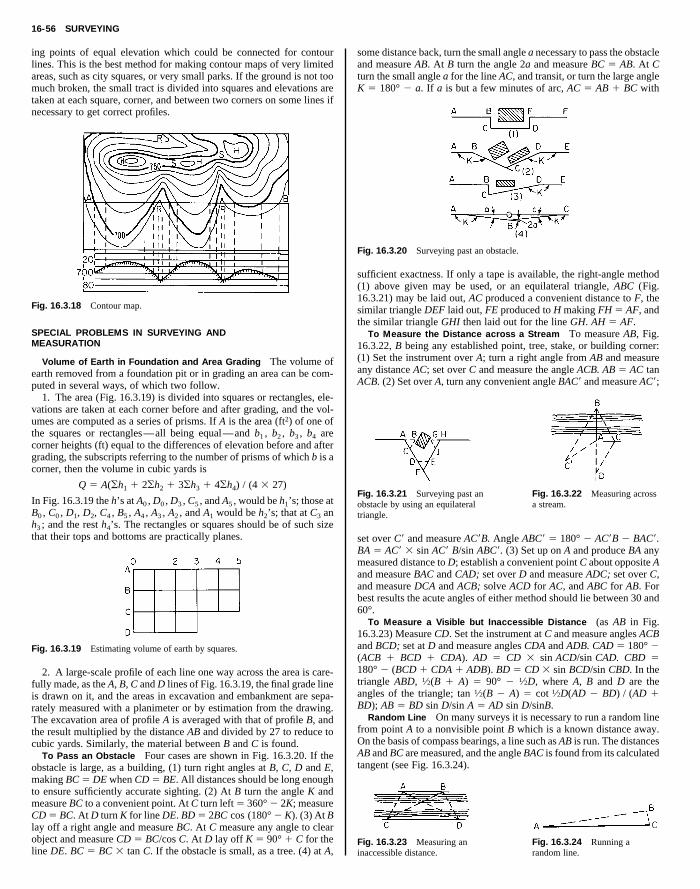
16-56 SURVEYING
ing points of equal elevation which could be connected for contourlines. This is the best method for making contour maps of very limitedareas, such as city squares, or very small parks. If the ground is not toomuch broken, the small tract is divided into squares and elevations aretaken at each square, corner, and between two corners on some lines ifnecessary to get correct profiles.
some distance back, turn the small angle a necessary to pass the obstacleand measure AB. At B turn the angle 2a and measure BC 5 AB. At Cturn the small angle a for the line AC, and transit, or turn the large angleK 5 180° 2 a. If a is but a few minutes of arc, AC 5 AB 1 BC with
Fig. 16.3.18 Contour map.
SPECIAL PROBLEMS IN SURVEYING ANDMEASURATION
Volume of Earth in Foundation and Area Grading The volume ofearth removed from a foundation pit or in grading an area can be com-puted in several ways, of which two follow.
1. The area (Fig. 16.3.19) is divided into squares or rectangles, ele-vations are taken at each corner before and after grading, and the vol-umes are computed as a series of prisms. If A is the area (ft2) of one ofthe squares or rectangles—all being equal—and b1 , b2 , b3 , b4 arecorner heights (ft) equal to the differences of elevation before and aftergrading, the subscripts referring to the number of prisms of which b is acorner, then the volume in cubic yards is
Q 5 A(oh1 1 2oh2 1 3oh3 1 4oh4) / (4 3 27)
In Fig. 16.3.19 the h’s at A0 , D0 , D3 , C5 , and A5 , would be h1’s; those atB0 , C0 , D1, D2, C4 , B5 , A4 , A3 , A2 , and A1 would be h2’s; that at C3 anh3 ; and the rest h4’s. The rectangles or squares should be of such sizethat their tops and bottoms are practically planes.
Fig. 16.3.19 Estimating volume of earth by squares.
2. A large-scale profile of each line one way across the area is care-fully made, as the A, B, C and D lines of Fig. 16.3.19, the final grade lineis drawn on it, and the areas in excavation and embankment are sepa-rately measured with a planimeter or by estimation from the drawing.The excavation area of profile A is averaged with that of profile B, andthe result multiplied by the distance AB and divided by 27 to reduce tocubic yards. Similarly, the material between B and C is found.
To Pass an Obstacle Four cases are shown in Fig. 16.3.20. If theobstacle is large, as a building, (1) turn right angles at B, C, D and E,making BC 5 DE when CD 5 BE. All distances should be long enoughto ensure sufficiently accurate sighting. (2) At B turn the angle K andmeasure BC to a convenient point. At C turn left 5 360°2 2K; measureCD 5 BC. At D turn K for line DE. BD 5 2BC cos (180°2 K). (3) At Blay off a right angle and measure BC. At C measure any angle to clearobject and measure CD 5 BC/cos C. At D lay off K 5 90° 1 C for theline DE. BC 5 BC 3 tan C. If the obstacle is small, as a tree. (4) at A,
Fig. 16.3.20 Surveying past an obstacle.
sufficient exactness. If only a tape is available, the right-angle method(1) above given may be used, or an equilateral triangle, ABC (Fig.16.3.21) may be laid out, AC produced a convenient distance to F, thesimilar triangle DEF laid out, FE produced to H making FH 5 AF, andthe similar triangle GHI then laid out for the line GH. AH 5 AF.
To Measure the Distance across a Stream To measure AB, Fig.16.3.22, B being any established point, tree, stake, or building corner:(1) Set the instrument over A; turn a right angle from AB and measureany distance AC; set over C and measure the angle ACB. AB 5 AC tanACB. (2) Set over A, turn any convenient angle BAC9 and measure AC9;
Fig. 16.3.21 Surveying past anobstacle by using an equilateraltriangle.
Fig. 16.3.22 Measuring acrossa stream.
set over C9 and measure AC9B. Angle ABC9 5 180° 2 AC9B 2 BAC9.BA 5 AC9 3 sin AC9 B/sin ABC9. (3) Set up on A and produce BA anymeasured distance to D; establish a convenient point C about opposite Aand measure BAC and CAD; set over D and measure ADC; set over C,and measure DCA and ACB; solve ACD for AC, and ABC for AB. Forbest results the acute angles of either method should lie between 30 and60°.
To Measure a Visible but Inaccessible Distance (as AB in Fig.16.3.23) Measure CD. Set the instrument at C and measure angles ACBand BCD; set at D and measure angles CDA and ADB. CAD 5 180° 2(ACB 1 BCD 1 CDA). AD 5 CD 3 sin ACD/sin CAD. CBD 5180° 2 (BCD 1 CDA 1 ADB). BD 5 CD 3 sin BCD/sin CBD. In thetriangle ABD, 1⁄2(B 1 A) 5 90° 2 1⁄2D, where A, B and D are theangles of the triangle; tan 1⁄2(B 2 A) 5 cot 1⁄2D(AD 2 BD) / (AD 1BD); AB 5 BD sin D/sin A 5 AD sin D/sinB.
Random Line On many surveys it is necessary to run a random linefrom point A to a nonvisible point B which is a known distance away.On the basis of compass bearings, a line such as AB is run. The distancesAB and BC are measured, and the angle BAC is found from its calculatedtangent (see Fig. 16.3.24).
Fig. 16.3.23 Measuring aninaccessible distance.
Fig. 16.3.24 Running arandom line.
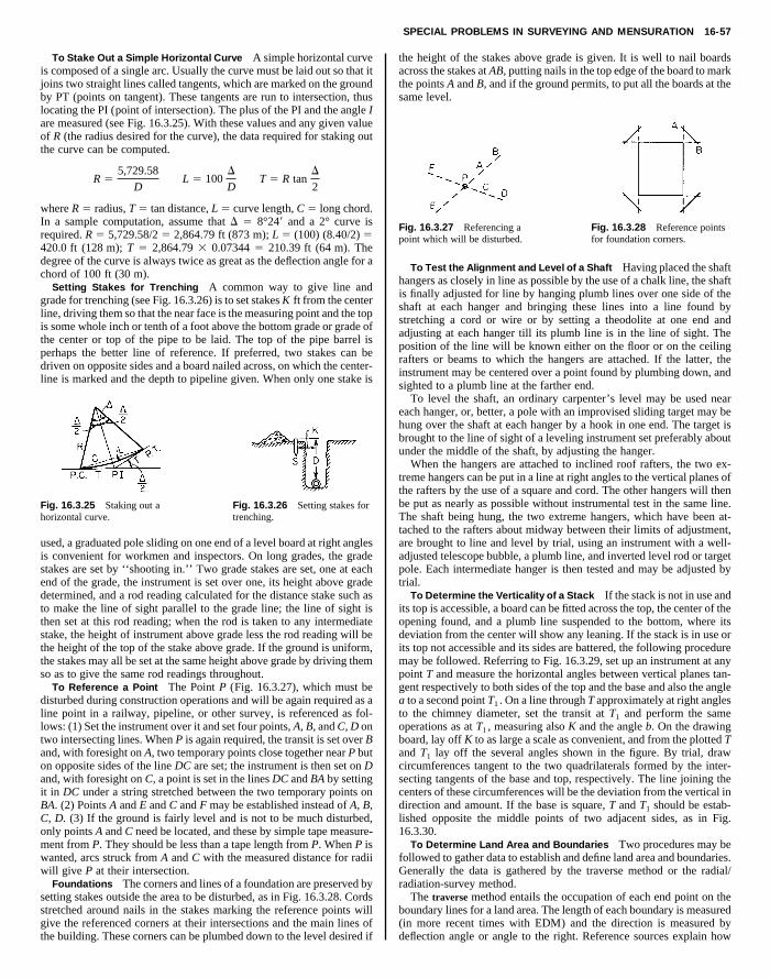
SPECIAL PROBLEMS IN SURVEYING AND MENSURATION 16-57
To Stake Out a Simple Horizontal Curve A simple horizontal curveis composed of a single arc. Usually the curve must be laid out so that itjoins two straight lines called tangents, which are marked on the groundby PT (points on tangent). These tangents are run to intersection, thuslocating the PI (point of intersection). The plus of the PI and the angle Iare measured (see Fig. 16.3.25). With these values and any given valueof R (the radius desired for the curve), the data required for staking outthe curve can be computed.
R 55,729.58
L 5 100D
T 5 R tanD
the height of the stakes above grade is given. It is well to nail boardsacross the stakes at AB, putting nails in the top edge of the board to markthe points A and B, and if the ground permits, to put all the boards at thesame level.
Copyright (C) 1999 by The McGraw-Hill Companies, Inc. All rights reserved. Use ofthis product is subject to the terms of its License Agreement. Click here to view.
D D 2
where R 5 radius, T 5 tan distance, L 5 curve length, C 5 long chord.In a sample computation, assume that D 5 8°249 and a 2° curve isrequired. R 5 5,729.58/2 5 2,864.79 ft (873 m); L 5 (100) (8.40/2) 5420.0 ft (128 m); T 5 2,864.79 3 0.07344 5 210.39 ft (64 m). Thedegree of the curve is always twice as great as the deflection angle for achord of 100 ft (30 m).
Setting Stakes for Trenching A common way to give line andgrade for trenching (see Fig. 16.3.26) is to set stakes K ft from the centerline, driving them so that the near face is the measuring point and the topis some whole inch or tenth of a foot above the bottom grade or grade ofthe center or top of the pipe to be laid. The top of the pipe barrel isperhaps the better line of reference. If preferred, two stakes can bedriven on opposite sides and a board nailed across, on which the center-line is marked and the depth to pipeline given. When only one stake is
Fig. 16.3.25 Staking out ahorizontal curve.
Fig. 16.3.26 Setting stakes fortrenching.
used, a graduated pole sliding on one end of a level board at right anglesis convenient for workmen and inspectors. On long grades, the gradestakes are set by ‘‘shooting in.’’ Two grade stakes are set, one at eachend of the grade, the instrument is set over one, its height above gradedetermined, and a rod reading calculated for the distance stake such asto make the line of sight parallel to the grade line; the line of sight isthen set at this rod reading; when the rod is taken to any intermediatestake, the height of instrument above grade less the rod reading will bethe height of the top of the stake above grade. If the ground is uniform,the stakes may all be set at the same height above grade by driving themso as to give the same rod readings throughout.
To Reference a Point The Point P (Fig. 16.3.27), which must bedisturbed during construction operations and will be again required as aline point in a railway, pipeline, or other survey, is referenced as fol-lows: (1) Set the instrument over it and set four points, A, B, and C, D ontwo intersecting lines. When P is again required, the transit is set over Band, with foresight on A, two temporary points close together near P buton opposite sides of the line DC are set; the instrument is then set on Dand, with foresight on C, a point is set in the lines DC and BA by settingit in DC under a string stretched between the two temporary points onBA. (2) Points A and E and C and F may be established instead of A, B,C, D. (3) If the ground is fairly level and is not to be much disturbed,only points A and C need be located, and these by simple tape measure-ment from P. They should be less than a tape length from P. When P iswanted, arcs struck from A and C with the measured distance for radiiwill give P at their intersection.
Foundations The corners and lines of a foundation are preserved bysetting stakes outside the area to be disturbed, as in Fig. 16.3.28. Cordsstretched around nails in the stakes marking the reference points willgive the referenced corners at their intersections and the main lines ofthe building. These corners can be plumbed down to the level desired if
Fig. 16.3.27 Referencing apoint which will be disturbed.
Fig. 16.3.28 Reference pointsfor foundation corners.
To Test the Alignment and Level of a Shaft Having placed the shafthangers as closely in line as possible by the use of a chalk line, the shaftis finally adjusted for line by hanging plumb lines over one side of theshaft at each hanger and bringing these lines into a line found bystretching a cord or wire or by setting a theodolite at one end andadjusting at each hanger till its plumb line is in the line of sight. Theposition of the line will be known either on the floor or on the ceilingrafters or beams to which the hangers are attached. If the latter, theinstrument may be centered over a point found by plumbing down, andsighted to a plumb line at the farther end.
To level the shaft, an ordinary carpenter’s level may be used neareach hanger, or, better, a pole with an improvised sliding target may behung over the shaft at each hanger by a hook in one end. The target isbrought to the line of sight of a leveling instrument set preferably aboutunder the middle of the shaft, by adjusting the hanger.
When the hangers are attached to inclined roof rafters, the two ex-treme hangers can be put in a line at right angles to the vertical planes ofthe rafters by the use of a square and cord. The other hangers will thenbe put as nearly as possible without instrumental test in the same line.The shaft being hung, the two extreme hangers, which have been at-tached to the rafters about midway between their limits of adjustment,are brought to line and level by trial, using an instrument with a well-adjusted telescope bubble, a plumb line, and inverted level rod or targetpole. Each intermediate hanger is then tested and may be adjusted bytrial.
To Determine the Verticality of a Stack If the stack is not in use andits top is accessible, a board can be fitted across the top, the center of theopening found, and a plumb line suspended to the bottom, where itsdeviation from the center will show any leaning. If the stack is in use orits top not accessible and its sides are battered, the following proceduremay be followed. Referring to Fig. 16.3.29, set up an instrument at anypoint T and measure the horizontal angles between vertical planes tan-gent respectively to both sides of the top and the base and also the anglea to a second point T1 . On a line through T approximately at right anglesto the chimney diameter, set the transit at T1 and perform the sameoperations as at T1 , measuring also K and the angle b. On the drawingboard, lay off K to as large a scale as convenient, and from the plotted Tand T1 lay off the several angles shown in the figure. By trial, drawcircumferences tangent to the two quadrilaterals formed by the inter-secting tangents of the base and top, respectively. The line joining thecenters of these circumferences will be the deviation from the vertical indirection and amount. If the base is square, T and T1 should be estab-lished opposite the middle points of two adjacent sides, as in Fig.16.3.30.
To Determine Land Area and Boundaries Two procedures may befollowed to gather data to establish and define land area and boundaries.Generally the data is gathered by the traverse method or the radial/radiation-survey method.
The traverse method entails the occupation of each end point on theboundary lines for a land area. The length of each boundary is measured(in more recent times with EDM) and the direction is measured bydeflection angle or angle to the right. Reference sources explain how
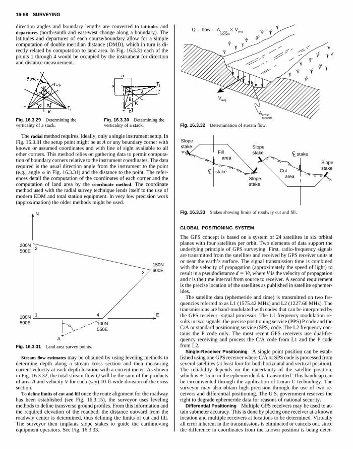
16-58 SURVEYING
direction angles and boundary lengths are converted to latitudes anddepartures (north-south and east-west change along a boundary). Thelatitudes and departures of each course/boundary allow for a simplecomputation of double meridian distance (DMD), which in turn is di-rectly related by computation to land area. In Fig. 16.3.31 each of thepoints 1 through 4 would be occupied by the instrument for directionand distance measurement.
Vavg3Q 5 flow 5 Acrosssection
Copyright (C) 1999 by The McGraw-Hill Companies, Inc. All rights reserved. Use ofthis product is subject to the terms of its License Agreement. Click here to view.
Fig. 16.3.29 Determining theverticality of a stack.
Fig. 16.3.30 Determining theverticality of a stack.
The radial method requires, ideally, only a single instrument setup. InFig. 16.3.31 the setup point might be at A or any boundary corner withknown or assumed coordinates and with line of sight available to allother corners. This method relies on gathering data to permit computa-tion of boundary corners relative to the instrument coordinates. The datarequired is the usual direction angle from the instrument to the point(e.g., angle a in Fig. 16.3.31) and the distance to the point. The refer-ences detail the computation of the coordinates of each corner and thecomputation of land area by the coordinate method. The coordinatemethod used with the radial survey technique lends itself to the use ofmodern EDM and total station equipment. In very low precision work(approximation) the older methods might be used.
200N500E
100N500E
150N600E
100N550E
2
1 E
A
4
3
N
a
Fig. 16.3.31 Land area survey points.
Stream flow estimates may be obtained by using leveling methods todetermine depth along a stream cross section and then measuringcurrent velocity at each depth location with a current meter. As shownin Fig. 16.3.32, the total stream flow Q will be the sum of the productsof area A and velocity V for each (say) 10-ft-wide division of the crosssection.
To define limits of cut and fill once the route alignment for the roadwayhas been established (see Fig. 16.3.15), the surveyor uses levelingmethods to define transverse ground profiles. From this information andthe required elevation of the roadbed, the distance outward from theroadway center is determined, thus defining the limits of cut and fill.The surveyor then implants slope stakes to guide the earthmovingequipment operators. See Fig. 16.3.33.
Vavg
Acrosssection
Fig. 16.3.32 Determination of stream flow.
Slopestake Slope
stakeFill area
Cut areaSlope
stake
CL
Slopestake
stake
CL stake
Fig. 16.3.33 Stakes showing limits of roadway cut and fill.
GLOBAL POSITIONING SYSTEM
The GPS concept is based on a system of 24 satellites in six orbitalplanes with four satellites per orbit. Two elements of data support theunderlying principle of GPS surveying. First, radio-frequency signalsare transmitted from the satellites and received by GPS receiver units ator near the earth’s surface. The signal transmission time is combinedwith the velocity of propagation (approximately the speed of light) toresult in a pseudodistance d 5 Vt, where V is the velocity of propagationand t is the time interval from source to receiver. A second requirementis the precise location of the satellites as published in satellite ephemer-ides.
The satellite data (ephemeride and time) is transmitted on two fre-quencies referred to as L1 (1575.42 MHz) and L2 (1227.60 MHz). Thetransmissions are band-modulated with codes that can be interpreted bythe GPS receiver–signal processor. The L1 frequency modulation re-sults in two signals: the precise positioning service (PPS) P code and theC/A or standard positioning service (SPS) code. The L2 frequency con-tains the P code only. The most recent GPS receivers use dual-fre-quency receiving and process the C/A code from L1 and the P codefrom L2.
Single-Receiver Positioning A single point position can be estab-lished using one GPS receiver where C/A or SPS code is processed fromseveral satellites (at least four for both horizontal and vertical position).The reliability depends on the uncertainty of the satellite position,which is 1 15 m in the ephemeride data transmitted. This handicap canbe circumvented through the application of Loran C technology. Thesurveyor may also obtain high precision through the use of two re-ceivers and differential positioning. The U.S. government reserves theright to degrade ephemeride data for reasons of national security.
Differential Positioning Multiple GPS receivers may be used to at-tain submeter accuracy. This is done by placing one receiver at a knownlocation and multiple receivers at locations to be determined. Virtuallyall error inherent in the transmissions is eliminated or cancels out, sincethe difference in coordinates from the known position is being deter-
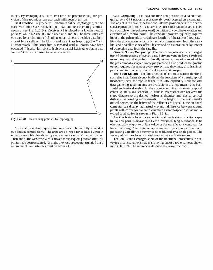
GLOBAL POSITIONING SYSTEM 16-59
mined. By averaging data taken over time and postprocessing, the pre-cision of this technique can approach millimeter precision.
Field Practice A procedure, sometimes called leapfrogging, can beused with three GPS receivers (R1, R2, and R3) operating simulta-neously (see Fig. 16.3.34). Receiver R1 is placed at a known controlpoint P, while R2 and R3 are placed at L and M. The three units areoperated for a minimum of 15 min to obtain time and position data fromat least four satellites. The R1 at P and R2 at L are leapfrogged to N andO respectively. This procedure is repeated until all points have beenoccupied. It is also desirable to include a partial leapfrog to obtain data
GPS Computing The data for time and position of a satellite ac-quired by a GPS station is subsequently postprocessed on a computer.The object is to convert the time and satellite-position data to the earth-surface position of the GPS receiver. At least four satellites are neededfor a complete (three-dimensional) definition of coordinate location andelevation of a control point. The computer program typically requiresinput of the ephemerides-coordinate location of the (at least) four satel-lites, the propagation velocity of the radio transmission from the satel-lite, and a satellite-clock offset determined by calibration or by receiptof correction data from the satellite.
Copyright (C) 1999 by The McGraw-Hill Companies, Inc. All rights reserved. Use ofthis product is subject to the terms of its License Agreement. Click here to view.
for the OP line if a closed traverse is wanted.
L
P
M
N
O
Fig. 16.3.34 Determining positions by leapfrogging.
A second procedure requires two receivers to be initially located attwo known control points. The units are operated for at least 15 min inorder to establish data defining the relative location of the two points.Then one of the GPS receivers is moved to subsequent positions until allpoints have been occupied. As in the previous procedure, signals from aminimum of four satellites must be acquired.
General Survey Computing The microcomputer is now an integralpart of the processing of survey data. Software vendors have developedmany programs that perform virtually every computation required bythe professional surveyor. Some programs will also produce the graphicoutput required for almost every survey: site drawings, plat drawings,profile and transverse sections, and topographic maps.
The Total Station The construction of the total station device issuch that it performs electronically all the functions of a transit, opticaltheodolite, level, and tape. It has built-in EDM capability. Thus the totaldata-gathering requirements are available in a single instrument: hori-zontal and vertical angles plus the distance from the instrument’s opticalcenter to the EDM reflector. A built-in microprocessor converts theslope distance to the desired horizontal distance, and also to verticaldistance for leveling requirements. If the height of the instrument’soptical center and the height of the reflector are keyed in, the on-boardcomputer can display that actual elevation difference between groundpoints with correction for earth curvature and atmospheric refraction. Atypical total station is shown in Fig. 16.3.11.
Another feature found in some total stations is data-collection capa-bility. This permits data as read by the instrument (angle, distance) to beelectronically output to a data collector for transfer to a computer forlater processing. A total station operating in conjunction with a remote-processing unit allows a survey to be conducted by a single person. Thevariety of features found on total station devices is enormous.
The total station changes some of the traditional procedures in sur-veying practice. An example is the laying out of a route curve as shownin Fig. 16.3.24. The references describe the newer methods.