insights into the geometry of the gaussian kernel and an ... · the geometry of problems formulated...

Insights into the Geometry of the Gaussian Kernel

and an Application in Geometric Modeling

Master Thesis

Michael Eigensatz

Advisor: Joachim Giesen

Professor: Mark Pauly

Swiss Federal Institute of Technology Zurich

March 13, 2006

Contents

1 Introduction 5

2 Kernels and Nonlinear Feature Maps 7

2.1 Nonlinear Feature Maps . . . . . . . . . . . . . . . . . . . . . . . . 7

2.2 Positive (Semi-)Definite Kernels . . . . . . . . . . . . . . . . . . . . 8

2.2.1 Gram Matrices and Positive Definiteness . . . . . . . . . . . 8

2.2.2 Kernel Induced Feature Spaces and the Kernel Trick . . . . 9

2.2.3 RBF Kernels . . . . . . . . . . . . . . . . . . . . . . . . . . 10

2.3 Conditionally Positive Semidefinite Kernels . . . . . . . . . . . . . 12

3 Surface Modeling with the SlabSVM 13

3.1 The SlabSVM . . . . . . . . . . . . . . . . . . . . . . . . . . . . . . 13

3.1.1 Problem Formulation . . . . . . . . . . . . . . . . . . . . . 13

3.1.2 The Solution of the SlabSVM . . . . . . . . . . . . . . . . . 15

3.1.3 The Geometry of the SlabSVM . . . . . . . . . . . . . . . . 22

3.2 The OpenSlabSVM . . . . . . . . . . . . . . . . . . . . . . . . . . . 22


3.2.2 The Solution of the OpenSlabSVM . . . . . . . . . . . . . . 24

3.2.3 The Geometry of the OpenSlabSVM Using the Gaussian Kernel 25

3.3 The ZeroSlabSVM . . . . . . . . . . . . . . . . . . . . . . . . . . . 27


3.3.2 The Solution of the ZeroSlabSVM . . . . . . . . . . . . . . 29

3.3.3 The Geometry of the ZeroSlabSVM Using the Gaussian Kernel 30

3.3.4 The ZeroSlabSVM and Shape Reconstruction Using Radial Basis Functions 32

3.3.5 Solving the ZeroSlabSVM . . . . . . . . . . . . . . . . . . . 33

3.4 The Geometry of the SlabSVM Revisited . . . . . . . . . . . . . . 34

4 Center-of-Ball Approximation Algorithm 37

4.1 The Algorithm . . . . . . . . . . . . . . . . . . . . . . . . . . . . . 37

4.1.1 Basic Two-Phase Iteration Algorithm . . . . . . . . . . . . 37

4.1.2 Geometric Interpretation . . . . . . . . . . . . . . . . . . . 38

4.1.3 Refined Algorithm . . . . . . . . . . . . . . . . . . . . . . . 40

4.2 Remarks . . . . . . . . . . . . . . . . . . . . . . . . . . . . . . . . . 42

3

4 CONTENTS

4.2.1 Convergence and Complexity . . . . . . . . . . . . . . . . . 424.2.2 Kernel Induced Feature Spaces . . . . . . . . . . . . . . . . 434.2.3 Off-Surface Points . . . . . . . . . . . . . . . . . . . . . . . 454.2.4 Orthogonalization . . . . . . . . . . . . . . . . . . . . . . . 47

4.3 Results . . . . . . . . . . . . . . . . . . . . . . . . . . . . . . . . . . 47

5 Feature-Coefficient Correlation 515.1 Features of a Shape . . . . . . . . . . . . . . . . . . . . . . . . . . . 515.2 Feature-Coefficient Correlation . . . . . . . . . . . . . . . . . . . . 51

Chapter 1

Introduction

Since the introduction of the Support Vector Machines, kernel techniques havebecome an important instrument for a number of tasks in machine learning andstatistics. Each kernel defines an implicit transformation from objective space intoa (usually higher dimensional) feature space. Depending on the chosen kernel, thegeometry of this induced feature space can be very specific. Using RBF kernelsfor example, the points in feature space all lie on a hypersphere around the origin.Our goal was to analyze the geometric constraints of the feature space inducedby a RBF kernel (and the Gaussian kernel in particular) and its implications onthe geometry of problems formulated with such kernels. We demonstrate in theexample of shape reconstruction using the SlabSVM that those implications canthen be used to restate or even improve algorithms performed in kernel featurespaces.Note that the techniques presented in this thesis as kernels or Support Vector Ma-chines, are mainly used in machine learning. However, our research focus is not somuch the analysis of learning related concepts (as risk and loss functions or otherelements of statistical learning theory) but rather to investigate the properties(especially the geometric ones) of these techniques and to gain insights possiblyleading to new perspectives.

Chapter 2 gives a short introduction into the basic concepts crucial for thesucceeding chapters as nonlinear feature maps and kernels. In chapter 3 the Slab-SVM is introduced as a method for shape reconstruction, along with a study ofthe solution properties, interesting special cases and geometric interpretations.Chapter 4 offers an in-depth analysis of a new algorithm for a special case of theSlabSVM, which exploits geometric insights gained so far.Finally, chapter 5 sheds some light on the interesting observation that the solutionof the SlabSVM seems to correlate with features of the shape as ridges, ravines orsharp edges.

5

6 CHAPTER 1. INTRODUCTION

Chapter 2

Kernels and Nonlinear FeatureMaps

2.1 Nonlinear Feature Maps

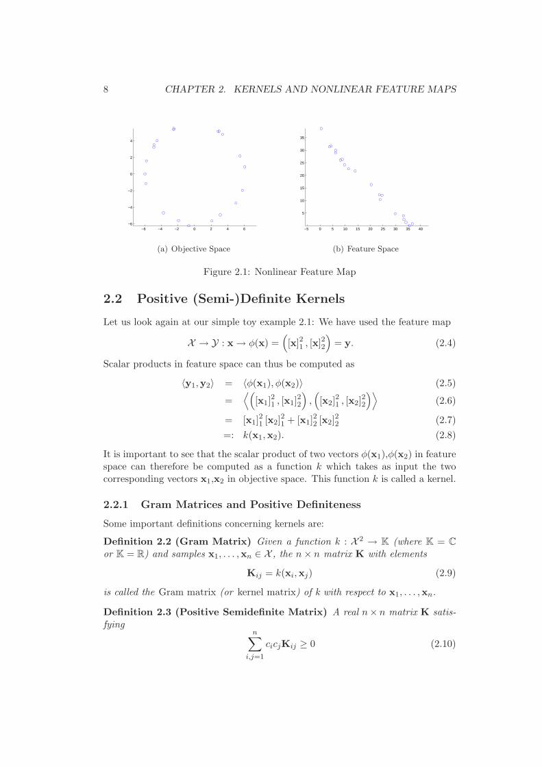
A nonlinear feature map can be written as a nonlinear transformation functionφ, which transforms any point x ∈ X to a corresponding point φ(x) ∈ Y. Thespace X of the original samples is then called objective space and Y is calledfeature space. Nonlinear feature maps can be useful for many applications. Thisis demonstrated by the following symbolic example:

Example 2.1 Given is a set of sample points xi = ([xi]1 , [xi]2) ∈ R2 approxi-

mately arranged on a circle around the origin (fig. 2.1(a)). We now want to fit acurve through these points. To this end, we apply the feature map

φ(x) =(

[x]21 , [x]22

)

∈ R2. (2.1)

In Objective space, points x on circles centered at the origin meet the condition

[x]21 + [x]22 = const. (2.2)

For the corresponding points φ(x) = y in feature space it consequently holds

[y]1 + [y]2 = const., (2.3)

which means that they lie on a straight line. Using the described feature map, thetransformed sample points will thus approximately form a linear shape in featurespace (fig. 2.1(b)), which is easier to learn.

Of course this simple toy example is somewhat artificial and it may seem oversim-plified. Nevertheless, it is sufficient to highlight the important fact that nonlinearfeature maps can linearize problems and therefore reduce their solution complexity.

7

8 CHAPTER 2. KERNELS AND NONLINEAR FEATURE MAPS

−6 −4 −2 0 2 4 6−6

−4

−2

0

2

4

(a) Objective Space

−5 0 5 10 15 20 25 30 35 40

5

10

15

20

25

30

35

(b) Feature Space

Figure 2.1: Nonlinear Feature Map

2.2 Positive (Semi-)Definite Kernels

Let us look again at our simple toy example 2.1: We have used the feature map

X → Y : x → φ(x) =(

[x]21 , [x]22

)

= y. (2.4)

Scalar products in feature space can thus be computed as

〈y1,y2〉 = 〈φ(x1), φ(x2)〉 (2.5)

=⟨(

[x1]21 , [x1]

22

)

,(

[x2]21 , [x2]

22

)⟩

(2.6)

= [x1]21 [x2]

21 + [x1]

22 [x2]

22 (2.7)

=: k(x1,x2). (2.8)

It is important to see that the scalar product of two vectors φ(x1),φ(x2) in featurespace can therefore be computed as a function k which takes as input the twocorresponding vectors x1,x2 in objective space. This function k is called a kernel.

2.2.1 Gram Matrices and Positive Definiteness

Some important definitions concerning kernels are:

Definition 2.2 (Gram Matrix) Given a function k : X 2 → K (where K = C

or K = R) and samples x1, . . . ,xn ∈ X , the n × n matrix K with elements

Kij = k(xi,xj) (2.9)

is called the Gram matrix (or kernel matrix) of k with respect to x1, . . . ,xn.

Definition 2.3 (Positive Semidefinite Matrix) A real n× n matrix K satis-fying

n∑

i,j=1

cicjKij ≥ 0 (2.10)

2.2. POSITIVE (SEMI-)DEFINITE KERNELS 9

for all ci ∈ R is called positive semidefinite. If equality in (2.10) only holds forc1 = . . . = cn = 0 then it is called positive definite.

Definition 2.4 (Positive Semidefinite Kernel) Let X be a nonempty set. Afunction k on X × X which for all n ∈ N and all x1, . . . ,xn ∈ X gives rise toa positive semidefinite Gram matrix is called a positive semidefinite kernel. Ifequality in (2.10) only holds for c1 = . . . = cn = 0 then it is called a positivedefinite kernel.

Note that positive definiteness is a special case of positive semidefiniteness andtherefore every property stated for positive semidefinite kernels also holds forpositive definite ones.Another class of kernels are the conditionally positive semidefinite kernels, definedin section 2.3, which play an important role in Computer Graphics. Since positive(semi)definite kernels give rise to nice geometric interpretations, they will be ourmain interest. Unless noted otherwise, a kernel will therefore always mean apositive (semi)definite kernel. However, we will discuss the use of conditionallypositive semidefinite kernels for surface reconstruction using radial basis functionswhen we study the ZeroSlabSVM in section 3.3.

2.2.2 Kernel Induced Feature Spaces and the Kernel Trick

In the beginning of this section we saw that we can compute scalar products inthe feature space of our simple toy example 2.1 by an evaluation of a kernel k onthe samples in objective space.In fact, for every positive semidefinite kernel it holds

k(x1,x2) = 〈φ(x1), φ(x2)〉 , (2.11)

for some feature map φ. It can therefore be stated that every positive semidefinitekernel implicitly defines a feature map φ into some Hilbert space. For our examplethis means that the kernel

k(x1,x2) = [x1]21 [x2]

21 + [x1]

22 [x2]

22 (2.12)

implicitly defines the feature map (2.4). This second statement indicates the powerof kernels: Let us assume we have given some sample points in objective spaceand we want to perform an algorithm on these samples (e.g. learning the shapedescribed by those samples). Since the structure of the samples is nonlinear, wewould like to apply a feature transformation φ into a feature space in order tolinearize the problem. Then we will perform the algorithm in feature space. Letus now further assume that this algorithm in feature space uses the scalar productas its sole basic operation. We know that there exists a kernel k, which implicitlydefines the used feature map φ and computes scalar products in the feature spaceas a function on points in the objective space. Using this kernel it is thus possible


to formulate our algorithm, which operates in feature space, directly in objectivespace, without the need of performing the feature transformation explicitly! Thiscan result in a massive reduction in complexity, especially when the feature spaceis very high (or even infinite) dimensional. An example of how this is done inpractice is the SlabSVM introduced in chapter 3.

Of course this ”Kernel Trick” only works when the algorithm in feature spaceonly depends on scalar products. Fortunately, due to the power of the scalarproduct, many interesting problems can be solved by algorithms fulfilling thiscondition. Consequently there exists quite a number of well-investigated kernelsused for a variety of problems in machine learning and many other fields. Thenext sections will introduce some kernels important for the following chapters. Foran in-depth analysis of kernels, their definitions and properties and applications,the interested reader is referred to the extensive literature including [1],[2],[3].

2.2.3 RBF Kernels

Radial basis function (RBF) kernels follow the form

k(x1,x1) = f (d(x1,x2)) (2.13)

where f is a function on R+0 and d is a metric in X , for which the usual choice is

d(x1,x2) = ‖x1 − x2‖ . (2.14)

The fact that for every metric d(x,x) = 0 gives rise to a first geometric statement:

Proposition 2.5 (Geometry of RBF Kernels) The transformed points φ(x)in the feature space induced by a positive semidefinite RBF kernel are equidistantto the origin and thus all lie on a hypersphere with radius k(x, x) = f(0) aroundthe origin.

The Gaussian Kernel

A very popular choice of a positive definite RBF kernel in machine learning is theGaussian kernel:

k(x1,x2) = exp

(

−‖x1 − x2‖

2

2σ2

)

, σ > 0. (2.15)

It was mentioned before that when using positive semidefinite RBF kernels thetransformed points in feature space all lie on a hypersphere around the origin. Forthe Gaussian kernel it holds

‖φ(xi)‖2 = 〈φ(xi), φ(xi)〉 = k(xi,xi) = 1. (2.16)

Therefore the hypersphere has radius one in this case.The Gaussian kernel has another very important property:

2.2. POSITIVE (SEMI-)DEFINITE KERNELS 11

Theorem 2.6 (Full Rank of Gaussian Gram Matrices)Suppose that x1, . . ., xn ∈ X are distinct points, and σ 6= 0. The matrix given by

Kij = exp

(

−‖xi − xj‖

2

2σ2

)

(2.17)

has full rank.

This leads to two crucial implications:

• The transformed feature points φ(x1), . . . , φ(xn) are linearly independent.

• In principle, the feature space induced by a Gaussian kernel is infinite dimen-sional. For geometric considerations however, it is usually sufficient to lookat the n dimensional subspace spanned by the feature points φ(x1), . . . , φ(xn).

The n points φ(xi) also lie on an n − 1 dimensional hyperball, which of courseis trivial since n linearly independent points always do. With only three points,the geometric setup in feature space is indicated in figure 2.2: The feature pointsφi = φ(xi), i = 1, 2, 3 lie on the three dimensional unit sphere around the originand can be interpolated by a circle on this sphere.

φ

φ

φ1

2

3

0

Figure 2.2: Feature space of Gaussian kernel with three sample points.


2.3 Conditionally Positive Semidefinite Kernels

Let us conclude the chapter with some notes on conditionally positive semidefinitekernels.

Definition 2.7 (Conditionally Positive Definite Kernels of Order q)A symmetric kernel X × X → R is called conditionally positive semidefinite oforder q on X ⊆ R

d if for any distinct points x1, . . . ,xn ∈ Rd it holds for the

quadratic formn∑

i,j=1

αiαjk(xi,xj) ≥ 0, (2.18)

provided that the coefficients α1, . . . , αn satisfy

n∑

i=1

αip(xi) = 0, (2.19)

for all polynomials p(x) on Rd of degree lower than q. If equality in (2.18) only

holds for α1 = . . . = αn = 0 then it is called conditionally positive definite.

Note that (unconditional) positive definiteness is identical to conditional positivedefiniteness of order zero and that conditional positive definiteness of order qimplies conditional positive definiteness of any larger order.Examples of conditionally positive definite radial kernels are:

k(x1,x2) = (−1)⌈β/2⌉(

c2 + ‖x1 − x2‖2)β/2

,

order q = ⌈β/2⌉ , β > 0, β /∈ 2N (2.20)

k(x1,x2) = (−1)k+1 ‖x1 − x2‖2k log ‖x1 − x2‖ ,

order q = k + 1, k ∈ N (2.21)

Conditionally positive semidefinite kernels of order larger than zero do not directlydefine a dot product in some feature space anymore and geometric considerationsof spaces induced by such kernels are not as straightforward as they are in the caseof order zero. Thus they are not the focus of this thesis. However, their use inthe context of shape reconstruction using radial basis functions will be discussedbriefly in subsection 3.3.4.

Chapter 3

Surface Modeling with theSlabSVM

This chapter studies shape reconstruction using the Slab Support Vector Machine(SlabSVM). Section 3.1 introduces the SlabSVM and shows some interesting as-pects and properties. As special cases of the SlabSVM, the OpenSlabSVM andZeroSlabSVM are presented in section 3.2 and 3.3 together with some relationsto shape reconstruction using radial basis functions as done in computer graphicsand geometric insights which will eventually lead to the algorithm introduced inchapter 4.

3.1 The SlabSVM

3.1.1 Problem Formulation

Assume we have given n sample points x1, . . . ,xn ∈ X as a sampling of an un-known shape, where usually but not necessarily X = R

2 or X = R3. We now want

to reconstruct this shape by learning a function f(x), which implicitly defines thelearned shape by one of its level-sets {x ∈ X : f(x) = c}. The SlabSVM was in-troduced in [4] as a kernel method for such an implicit surface modeling. Withoutthe use of outliers it can be stated as the optimization problem

minw,ρ

1

2‖w‖2 − ρ (3.1)

s.t. δ ≤ 〈w, φ(xi)〉 − ρ ≤ δ∗, ∀i (3.2)

defining the following geometric setup (fig. 3.1):We first apply a feature map φ(x) in order to linearize the problem. We will

later see that it will not be necessary to perform this transformation explicitly,since the kernel trick will be applicable (read chapter 2 for an introduction ofthese important concepts). The goal is then to find a slab, defined by two parallelhyperplanes orthogonal to the solution vector w, enclosing all the sample points

13

14 CHAPTER 3. SURFACE MODELING WITH THE SLABSVM

o

o

w

o

o

o

o

o

||w||(ρ+δ)/

.

||w||(ρ+δ )/*

Figure 3.1: Setup SlabSVM

φ(xi). The width of the slab has to be given in advance. Having found the solutionvector w, we can then reconstruct the shape as a level-set of the function

f(x) = 〈w, φ(x)〉 . (3.3)

In feature space, this represents a hyperplane parallel to those defining the slab.The level-set value is usually chosen such that this hyperplane lies within the slab,which holds for values in the interval [ρ + δ, ρ + δ∗]. Also for the evaluation of thefunction f , the use of a kernel will be of great help, as shown later.

To solve the optimization problem (3.1)-(3.2) we compute the generalized La-grangian function as

L(w, ρ,α, α∗) =1

2‖w‖2 − ρ −

n∑

i=1

αi (〈w, φ(xi)〉 − ρ − δ)

+

n∑

i=1

α∗i (〈w, φ(xi)〉 − ρ − δ∗) . (3.4)

The solution of our primal optimization problem is then equivalent to the one ofthe Lagrangian dual problem defined as

maxα,α∗

θ(α, α∗) (3.5)

subject to α ≥ 0 (3.6)

α∗ ≥ 0, (3.7)

where θ(α, α∗) = infw,ρ L(w, ρ,α, α∗).To compute the infimum of L with respect to the primal variables w and ρ we setthe corresponding derivatives to zero

∂L(w, ρ,α, α∗)

∂w= 0 ⇒ w =

n∑

i=1

(αi − α∗i ) φ(xi) (3.8)

3.1. THE SLABSVM 15

∂L(w, ρ,α, α∗)

∂ρ= 0 ⇒

n∑

i=1

(αi − α∗i ) = 1 (3.9)

and use the resulting equations to replace the primal variables in L by functionsof the dual variables αi and α∗

i . The dual problem can then be formulated as

minα,α∗

1

2

n∑

i,j=1

(αi − α∗i )(αj − α∗

j

)〈φ(xi), φ(xj)〉

− δ

n∑

i=1

αi + δ∗n∑

i=1

α∗i (3.10)

s.t. α(∗) ≥ 0 (3.11)

andn∑

i=1

(αi − α∗i ) = 1. (3.12)

Since the only operation performed on the feature points φ(xi) is the scalar prod-uct, we can apply the kernel trick and replace it by kernel evaluations, which leadsto the final problem formulation of the SlabSVM:

minα,α∗

1

2

n∑

i,j=1

(αi − α∗i )(αj − α∗

j

)k(xi,xj) − δ

n∑

i=1

αi + δ∗n∑

i=1

α∗i (3.13)

s.t. α(∗) ≥ 0 (3.14)

andn∑

i=1

(αi − α∗i ) = 1. (3.15)

This is a good example of how the use of kernels saves us from having to com-pute the feature map φ explicitly, because it does not appear in the optimizationproblem anymore. Instead, the feature transformation is implicitly defined by thechosen kernel k.The result is a convex quadratic program, which can be solved using standardtechniques.

3.1.2 The Solution of the SlabSVM

As mentioned earlier, the shape is reconstructed as a level-set of the function f(equation (3.3)). Since f too is defined only using scalar products, the use ofkernels becomes possible also here and with equation (3.8) we get

f(x) = 〈w, φ(x)〉 (3.16)

=

⟨n∑

i=1

(αi − α∗i )φ(xi), φ(x)

⟩

(3.17)

=n∑

i=1

(αi − α∗i ) 〈φ(xi), φ(x)〉 (3.18)


=n∑

i=1

(αi − α∗i ) k(xi,x). (3.19)

Thus, an explicit transformation into the feature space is at no point neededwhen reconstructing a shape with the SlabSVM, since we can perform all itscomputations directly in objective space.

Properties of the Solution Using a Gaussian Kernel

When we use a Gaussian kernel, the solution function f becomes

f(x) =n∑

i=1

(αi − α∗i ) exp

(

−‖xi − x‖2

2σ2

)

. (3.20)

There is a ”Gaussian Bell” located at each sample point xi contributing to theoverall value of f . The kernel parameter sigma controls the breadth of thosebells, also called the support of the kernel. The dual variables αi and α∗

i specifythe amount of the contribution of the bell located at sample point xi to f . Thereconstructed shape is then a level-set of this weighted sum of Gaussians. Tostudy some interesting properties of such a sum, let us investigate the followingexample:

Example 3.1 (Circular shape in 2D) Given samples x1, . . . ,xn ∈ R2, n ≥ 2

uniformly arranged on a circle with radius r around the origin (fig. 3.2):

xi =

(r cos

(2πn (i − 1)

)

r sin(

2πn (i − 1)

)

)

, where i = 1, . . . , n (3.21)

To interpolate these points with a level-set of a function described by equation(3.20), we can choose uniform weights 1 (remember that they have to fulfill equa-tion (3.15)):

(αi − α∗i ) =

1

n. (3.22)

Proof: Due to the symmetry of the setup, the function f(x) will take the samevalue at each sample point xi and therefore the shape defined by the level-set{x : f(x) = f(xi)} for any i will interpolate every sample point correctly. q.e.d.

The resulting function f is therefore

f(x) =1

n

n∑

i=1

exp

−

∥∥∥∥

(r cos

(2πn (i − 1)

)

r sin(

2πn (i − 1)

)

)

− x

∥∥∥∥

2

2σ2

(3.23)

1This would actually be the result of the ZeroSlabSVM applied to this setup, which is explainedin section 3.3.

3.1. THE SLABSVM 17

-4 4

x1

x2

60

-4

2

-6

2

-6

6

-2

-2

4

0

Figure 3.2: Points uniformly distributed on a circle.

and only depends on the number of sampling data n, the circle radius r and thekernel parameter σ. Figure 3.3 shows the plot of such a function for some values ofthe remaining parameters. Considering the level-sets of f for different parametervalues, two cases can be observed:

1. The function f decreases again and forms a valley in the middle of thecircle, causing a second (inner) ring to appear in the level-set (figures 3.3(a)-3.3(d)).

2. The function does not sink below the level-set value again in the middle ofthe circle and thus only the outer, point-interpolating ring lies in the level-set(figures 3.3(e)-3.3(f)).

Restating f to

f(x) =1

n

n∑

i=1

exp

−

r2

∥∥∥∥

(cos(

2πn (i − 1)

)

sin(

2πn (i − 1)

)

)

− x

r

∥∥∥∥

2

2σ2

, (3.24)

one can easily see that σ has the exact inverse influence to f as r has, when werescale with each change of r the evaluation points x such that they occupy the samerelative position with respect to the circle. Thus, for the qualitative description off , increasing r has the same effect as decreasing σ.In order to investigate the two observed cases in a more mathematical manner, letus compare the values of f at a sample point and the value of f at the origin (the


-8-8

-4

0.04

-4

00x1

0.08

x244

88

0.12

0.16

(a) σ = 2.5

x1

x2

60

2

-4

-6

4

2

6

-2

-2

-6

4

0-4

(b)

-8-8

-4-4

0.1

00x1x2

0.15

44

88

0.2

0.25

(c) σ = 3.5

-6

0-4

x1

x2

4-6 60

2

4

-2

6

-2

2

-4

(d)

-8-80.15

-4

0.2

-4

0.25

00x1x2

0.3

44

0.35

88

0.4

0.45

(e) σ = 5

x1

4

2

x2

640

-6

-4

6

-2

-2-6

-4

20

(f)

Figure 3.3: The function f with r = 6, n = 8 and different values for σ and thecorresponding reconstructed shapes.

3.1. THE SLABSVM 19

center of the circle). At the center, f becomes

f((0, 0)) =1

n

n∑

i=1

exp

−

r2

∥∥∥∥

(cos(

2πn (i − 1)

)

sin(

2πn (i − 1)

)

)∥∥∥∥

2

2σ2

(3.25)

=1

n

n∑

i=1

exp

(

−r2

2σ2

)

(3.26)

= exp

(

−r2

2σ2

)

. (3.27)

Since f takes on the same value for every sample point, we are free to choose apoint, for example x1 = (r, 0):

f((r, 0)) =1

n

n∑

i=1

exp

−

r2

∥∥∥∥

(cos(

2πn (i − 1)

)

sin(

2πn (i − 1)

)

)

−

(10

)∥∥∥∥

2

2σ2

(3.28)

=1

n

n∑

i=1

exp

(

−r2(2 − 2 cos

(2πn (i − 1)

))

2σ2

)

(3.29)

=1

nexp

(

−r2

2σ2

) n∑

i=1

exp

(

r2(2 cos

(2πn (i − 1)

)− 1)

2σ2

)

(3.30)

= f((0, 0))1

n

n∑

i=1

exp

((rσ

)2 (2 cos

(2πn (i − 1)

)− 1)

2

)

(3.31)

=: f((0, 0)) g(

n,r

σ

)

. (3.32)

We derived that f((r, 0)) has the value f((0, 0)) multiplied by a factor g which isa function in n and r

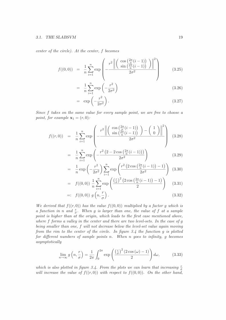
σ . When g is larger than one, the value of f at a samplepoint is higher than at the origin, which leads to the first case mentioned above,where f forms a valley in the center and there are two level-sets. In the case of gbeing smaller than one, f will not decrease below the level-set value again movingfrom the rim to the center of the circle. In figure 3.4 the function g is plottedfor different numbers of sample points n. When n goes to infinity, g becomesasymptotically

limn→∞

g(

n,r

σ

)

=1

2π

∫ 2π

0exp

((rσ

)2(2 cos (ω) − 1)

2

)

dω, (3.33)

which is also plotted in figure 3.4. From the plots we can learn that increasing rσ

will increase the value of f((r, 0)) with respect to f((0, 0)). On the other hand,


2

2

1.5

1

1.50.5

10.50

g

3

r / sigma

2.5

n=2

n=3

n=4

n=5

n->inf

Figure 3.4: The function g for different values of n.

when rσ lies in the range of 0 and about 1 to 1.7 (depending on n) f((r, 0)) will be

less than f((0, 0)). Thus, increasing σ or decreasing r will change f from a valley-type structure into more of a hill-type one and it will make the second, inner ringdisappear from the level-set. It will also smoothen the outer ring of the level-set.

Let us conclude this example with an analysis of one last question: We saw thatfor a certain range of r

σ f gets a hill-type structure and the inner ring observedearlier (fig. 3.3) disappears from our level-set. Is it also possible to increase r

σenough, such that the inner and outer rings of our level-set coincide? In thequalitative geography of f this would mean that the level-set lies exactly on theridge of the hills arranged around the circle and forming the valley in its center(figures 3.3(a) and 3.3(c)). To investigate this matter we form the gradient of fat an arbitrary sample point, for example at x1 = (r, 0):

∂f(x)

[x]1

∣∣∣∣x=(r,0)

=

r

nσ2

n∑

i=1

(

cos

(2π(i − 1)

n

)

− 1

)

exp

r2(

cos(

2π(i−1)n

)

− 1)

σ2

(3.34)

3.1. THE SLABSVM 21

∂f(x)

[x]2

∣∣∣∣x=(r,0)

=

r

nσ2

n∑

i=1

sin

(2π(i − 1)

n

)

exp

r2(

cos(

2π(i−1)n

)

− 1)

σ2

. (3.35)

Due to the symmetry of the problem and because n ≥ 2 equation (3.35) will alwaysbe zero. Since exp(x) > 0 and

(

cos

(2π(i − 1)

n

)

− 1

)

≤ 0, i = 1, . . . , n (3.36)

where equality only holds for i = 1, equation (3.34) will always be less than zerofor n ≥ 2. Therefore the gradient always points to the center of the circle andhas a nonzero length. This proves that f cannot have a maximum at any samplepoint and thus the case that the level-set lies exactly on the ridge of f cannot occur.Equation (3.34) also tells us that for very high values of r

σ the gradient will be verysmall and in any numerical setup the case becomes possible. However, when weincrease r

σ too much with respect to the number of sample points, the learned shapewill fall apart into several subshapes (fig. 3.5), which is usually not a satisfactoryresult.

-8-80.02

-4-4

0.04

00

0.06

x1x2

0.08

44

0.1

88

0.12

0.14

0.16

(a) σ = 2.3

x1

4

2

x2

640

-6

-4

6

-2

-2-6

-4

20

(b)

Figure 3.5: For too small values of rσ the reconstructed shape falls apart.

This extensive example reveals quite a number of interesting properties of thesolution as a level-set of a weighted sum of Gaussians. Of course all the com-putations only hold for a uniform sampling of circles but they provide insightsand intuitions very useful to understand the solutions for arbitrary shapes. Welearned for example that for certain parameter settings the resulting level-set can


contain additional shapes (as the additional inner ring in the example) or evendisintegrate, which we actually wish to avoid. This can be done by increasing thevalue of σ and changing f from a valley-type to a hill-type structure. Also, toalgorithmically find the level-set (i.e. in a rendering process) such a hill-structurewould be preferable, since level-sets are better found when the function is steeparound the iso-value. Unfortunately, as will be discussed later, increasing σ usu-ally introduces severe numerical difficulties and thus reduces the quality of thereconstructed shape.

3.1.3 The Geometry of the SlabSVM

Until now we have not yet studied the geometric implications to the SlabSVMwhen using feature spaces induced by specific kernels, as for example the Gaus-sian kernel. To do so, we will first consider some interesting special cases of theSlabSVM in the following sections. We will then return to the SlabSVM in sec-tion 3.4 and try to incorporate the insights from these special cases into a furtheranalysis of the SlabSVM itself.

3.2 The OpenSlabSVM


In section 3.1 we defined the SlabSVM as finding a slab, such that all sample pointsin feature space lie within this slab and its distance to the origin is maximal. Thespecial case presented in the current section is the one when the slab width isset to infinity. We have therefore only one remaining hyperplane to consider, forwhich we request that all the sample points lie on its side not containing the origin.Again, its distance to the origin is maximized (fig. 3.6). We therefore want tosolve the following optimization problem:

o

o

w

o

o

o

o

o.

||w||ρ /

Figure 3.6: Setup OpenSlabSVM

3.2. THE OPENSLABSVM 23

minw,ρ

1

2‖w‖2 − ρ (3.37)

s.t. 〈w, φ(xi)〉 ≥ ρ, ∀i (3.38)

As before, the sample points in objective space are denoted x1, . . . ,xn ∈ X andφ : X → Y is a feature map into some feature space.In machine learning, this problem is also called the OneClassSVM or Single-ClassSVM [1].To solve the problem, we can again form the generalized Lagrangian

L(w, ρ,α) =1

2‖w‖2 − ρ −

n∑

i=1

αi (〈w, φ(xi)〉 − ρ) (3.39)

set its derivatives to zero

∂L(w, ρ,α)

∂w= 0 ⇒ w =

n∑

i=1

αiφ(xi) (3.40)

∂L(w, ρ,α)

∂ρ= 0 ⇒

n∑

i=1

αi = 1 (3.41)

and state the dual problem

minα

1

2

n∑

i,j=1

αiαj 〈φ(xi), φ(xj)〉 (3.42)

s.t. α ≥ 0 (3.43)

andn∑

i=1

αi = 1. (3.44)

Again, we can use the kernel trick to replace the scalar products, which ultimatelyleads to the problem

minα

1

2

n∑

i,j=1

αiαjk(xi,xj) (3.45)

s.t. α ≥ 0 (3.46)

andn∑

i=1

αi = 1. (3.47)

As for the SlabSVM we have found a convex quadratic program to solve theOpenSlabSVM.


5 10 15 20 25 30

5

10

15

20

25

Figure 3.7: Solution of an OpenSlabSVM.

3.2.2 The Solution of the OpenSlabSVM

The solution of the OpenSlabSVM is the hyperplane defined by

〈w, φ(x)〉 = ρ, (3.48)

fulfilling the conditions stated in equations (3.37) - (3.38). In objective space, thepoints x for which (3.48) holds will not necessarily form a hyperplane anymore.They will rather define an arbitrary nonlinear shape enclosing the sample pointsxi (fig. 3.7).Using (3.40) this shape is defined as a level-set of the function

f(x) =

⟨n∑

i=1

αiφ(xi), φ(x)

⟩

(3.49)

=n∑

i=1

αi 〈φ(xi), φ(x)〉 (3.50)

=n∑

i=1

αik(xi,x). (3.51)

Note that the use of kernels here, and for the quadratic program in the last sub-section, once more saved us from having to compute any feature transformationdirectly. The level-set value is ρ, which can be computed by

ρ = mini

f(xi) (3.52)

since it is the lower bound of the inequality (3.38) and because there will alwaysbe a sample point where equality holds.Using a Gaussian kernel, f will again be a weighted sum of Gaussians as discussedin subsection 3.1.2.

3.2. THE OPENSLABSVM 25

φ

φ

φ

w1

2

3

0

Figure 3.8: Geometric setup of the OpenSlabSVM in Gaussian feature space withthree sample points.

3.2.3 The Geometry of the OpenSlabSVM Using the GaussianKernel

When we combine equation (3.40) and the quadratic program obtained at the endof subsection 3.2.1 we get another optimization problem for the OpenSlabSVM,namely

minw

1

2‖w‖2 (3.53)

s.t. α ≥ 0 (3.54)∑

i

αi = 1 (3.55)

w =∑

i

αiφ(xi). (3.56)

This alternative formulation reveals some nice geometric insights into the solutionw in feature space (fig. 3.8):

• Equation (3.56) tells us that w is a linear combination of the feature pointsφ(xi). The constraints (3.54) and (3.55) on the coefficients αi of this linearcombination narrow the solution region of w to points in the convex hull ofthe feature points φ(xi).

• Because of the objective function (3.53), w will be the point closest to theorigin in this convex hull.


There is another interesting geometric property of the OpenSlabSVM when thefeature map φ is defined implicitly by a Gaussian kernel:

Proposition 3.2 (OpenSlabSVM - MiniBall Analogy) In the feature spaceinduced by a Gaussian kernel, solving the OpenSlabSVM (which means finding thepoint w ∈ ConvexHull({φ(xi)}) closest to the origin) is equivalent to finding thecenter w of the minimal enclosing ball for the points φ(xi).

In fact, this analogy even holds for positive semidefinite RBF kernels in general.

Proof: The validity of this geometric analogy could actually be read off directlyfrom the implications of proposition 2.5 on the geometric setup. For a mathemat-ical proof let us state the problem of finding the center of the minimal enclosingball of the points φ(xi) as

minR∈R,w

R2 (3.57)

s.t. ‖φ(xi) − w‖2 ≤ R2, ∀i. (3.58)

We can express the squared norm in (3.58) by dot products

‖φ(xi) − w‖2 = 〈φ(xi), φ(xi)〉 + 〈w,w〉 − 2 〈φ(xi),w〉 (3.59)

As done before, we state the generalized Lagrangian as

L(w, R, α) = R2 − R2n∑

i=1

αi + 〈w,w〉n∑

i=1

αi +

n∑

i=1

αi 〈φ(xi), φ(xi)〉 − 2n∑

i=1

αi 〈φ(xi),w〉 , (3.60)

set its partial derivatives with respect to the primal variables to zero

∂L(w, R, α)

∂R= 0 ⇒

n∑

i=1

αi = 1 (3.61)

∂L(w, R, α)

∂w= 0 ⇒ w =

n∑

i=1

αiφ(xi), (3.62)

use the resulting equations to substitute the primal variables and introduce akernel to compute the dot product. The resulting dual problem then becomes:

minα

n∑

i,j=1

αiαjk(φ(xi), φ(xj)) −

n∑

i=1

αik(φ(xi), φ(xi)) (3.63)

s.t. α ≥ 0 (3.64)

andn∑

i=1

αi = 1 (3.65)

3.3. THE ZEROSLABSVM 27

Because of proposition 2.5, using an RBF kernel will render the linear term in theobjective function (3.63) constant and it is easy to see that as a consequence theMiniBall problem stated with (3.63)-(3.65) and its solution (3.62) become equiv-alent to the OpenSlabSVM defined in (3.45)-(3.47) and (3.40). q.e.d.

Taking these geometric insights into account, an alternative approach to theOpenSlabSVM could be a geometric algorithm solving the corresponding Mini-Ball problem, which is well studied in theoretical computer science (i.e. [5]).

3.3 The ZeroSlabSVM


In the last section we presented the OpenSlabSVM as a special case of the Slab-SVM when the slab width is set to infinity. Let us now consider the other extremecase reducing the slab width to zero and call that case the ZeroSlabSVM. Thiscan be formulated as to find a hyperplane orthogonal to w ∈ Y which exactlyinterpolates the sample points φ(x1), . . . , φ(xn) ∈ Y and has maximal distance tothe origin (fig. 3.9). Because of the nonlinear feature map φ : X → Y the samples

o

o

w

o

o

o

o

o

.

||w||ρ /

Figure 3.9: Setup ZeroSlabSVM

x1, . . . ,xn ∈ X in objective space do not necessarily have to form a linear shape.In the context of geometric modeling and shape reconstruction, the ZeroSlabSVMseems more interesting than the OpenSlabSVM, since the learned shape will in-terpolate the given sample points exactly.The problem of the ZeroSlabSVM can be stated as

minw,ρ

1

2‖w‖2 − ρ (3.66)

s.t. 〈w, φ(xi)〉 = ρ, ∀i. (3.67)

Note that the only difference to the OpenSlabSVM is an equality in (3.67) insteadof the inequality in (3.38). Because of this, only equality constraints are involved


and solving the problem with Lagrangian optimization theory becomes easier:Necessary and sufficient conditions for the solution are that the partial derivativesof the Lagrangian function

L(w, ρ,α) =1

2‖w‖2 − ρ −

n∑

i=1

αi (〈w, φ(xi)〉 − ρ) (3.68)

be zero. Thus:

∂L(w, ρ,α)

∂w= 0 ⇒ w =

n∑

i=1

αiφ(xi) (3.69)

∂L(w, ρ,α)

∂ρ= 0 ⇒

n∑

i=1

αi = 1 (3.70)

∂L(w, ρ,α)

∂αj= 0 ⇒ 〈w, φ(xj)〉 = ρ (3.71)

⇒n∑

i=1

αi 〈φ(xi), φ(xj)〉 = ρ, ∀j (3.72)

By introducing a variable transformation

βi :=αi

ρ(3.73)

and replacing the scalar product with a kernel, we get the new system of equations

w =∑

i

αiφ(xi) (3.74)

α = ρβ (3.75)n∑

i=1

βi =1

ρ(3.76)

n∑

i=1

βik(xi,xj) = 1, ∀j. (3.77)

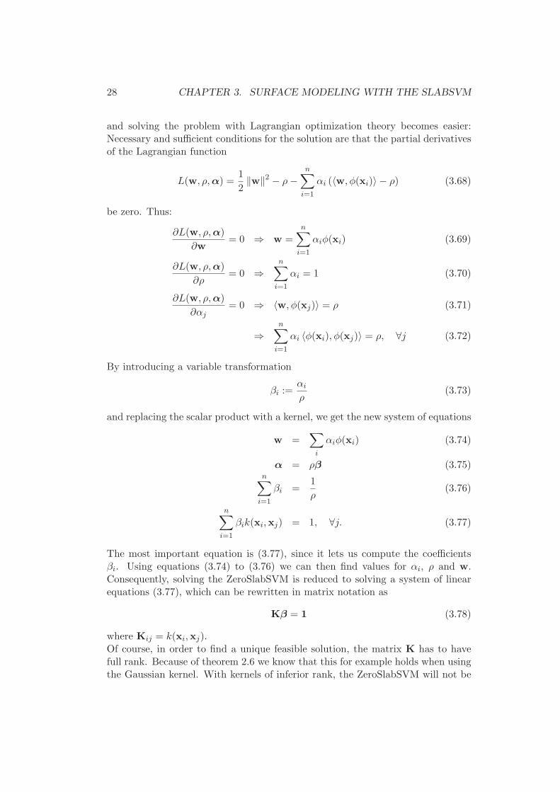
The most important equation is (3.77), since it lets us compute the coefficientsβi. Using equations (3.74) to (3.76) we can then find values for αi, ρ and w.Consequently, solving the ZeroSlabSVM is reduced to solving a system of linearequations (3.77), which can be rewritten in matrix notation as

Kβ = 1 (3.78)

where Kij = k(xi,xj).Of course, in order to find a unique feasible solution, the matrix K has to havefull rank. Because of theorem 2.6 we know that this for example holds when usingthe Gaussian kernel. With kernels of inferior rank, the ZeroSlabSVM will not be


solvable (except with the trivial solution w = 0 2). This can also be understoodin the geometry of the kernel induced feature space: The ZeroSlabSVM tries tointerpolate the endpoints of n vectors in the space spanned by the vectors by ahyperplane. In general this is only possible if the vectors are linearly independent,i.e., their endpoints are affinely independent and define a hyperplane. A necessaryand sufficient condition for the linear independence of the samples in a kernelinduced feature space is the full rank of its kernel.

3.3.2 The Solution of the ZeroSlabSVM

The solution of the ZeroSlabSVM is the hyperplane defined by

〈w, φ(x)〉 = ρ (3.79)

interpolating the sample points φ(x1), . . . , φ(xn) in feature space. In objectivespace, this hyperplane corresponds to a more complex shape interpolating theoriginal sample points x1, . . . ,xn. Using (3.69) it can be computed as the level-setof the function

f(x) =

⟨n∑

i=1

αiφ(xi), φ(x)

⟩

(3.80)

=n∑

i=1

αi 〈φ(xi), φ(x)〉 (3.81)

=n∑

i=1

αik(xi,x). (3.82)

Once more the use of kernels here and for the linear equation system in the lastsubsection saved us from having to compute any feature transformation explicitlywhen solving the ZeroSlabSVM, since all computations can be performed directlyin objective space. The level-set value is ρ, which can be computed for examplewith (3.76).Using a Gaussian kernel, f will again be a weighted sum of Gaussians as discussedin subsection 3.1.2. The solution (3.22) suggested in example 3.1 was in fact thesolution of the ZeroSlabSVM applied to the 2D-circle scenario, since the resultingshape interpolated all the points exactly. It should now be clear that when thesetup is as symmetric as it was in example 3.1, the rows of the matrix K aresimply permutations of each other and thus choosing the weights uniformly willsolve the system of linear equations (3.78).

2In this case the variable transformation (3.73) is no longer valid and (3.78) does not holdanymore, since ρ = 0.


3.3.3 The Geometry of the ZeroSlabSVM Using the GaussianKernel

Let us consider an approach to the problem of the ZeroSlabSVM (3.66)-(3.67)slightly different than the one in the last subsection. Again using Lagrangianoptimization theory and equations (3.68),(3.69) and (3.70) we can formulate itsdual problem:

minw

1

2‖w‖2 (3.83)

s.t.∑

i

αi = 1 (3.84)

w =∑

i

αiφ(xi) (3.85)

As for the OpenSlabSVM, this alternative formulation leads to some interestinginsights into the geometry of the ZeroSlabSVM. In fact, if we compare (3.83)-(3.85) with (3.53)-(3.56) from subsection 3.2.3 they look surprisingly similar. Theonly difference is the missing nonnegativity constraint (3.54) on the dual variablesin the case of the ZeroSlabSVM. Therefore the only consequence of changing theinequality of the OpenSlabSVM in (3.38) to an equality for the ZeroSlabSVMin (3.67) is the loss of this nonnegativity constraint. What are the geometricimplications of this observation? The alternative formulation of the ZeroSlabSVMstated above gives rise to the following geometric properties (fig. 3.10):

• Because of (3.85), w is a linear combination of the feature points φ(xi).(3.84) restricts w to lie in the affine hull of the feature points φ(xi) (comparedto the convex hull for the OpenSlabSVM).

• Because of the objective function (3.83), w will be the point closest to theorigin. Therefore it will be the projection of the origin onto the affine hullof {φ(xi)}.

In subsection 3.2.3 we proved the analogy of the OpenSlabSVM and the MiniBallproblem, when a Gaussian kernel is used. For the ZeroSlabSVM, a very similarstatement can be made:

Proposition 3.3 (ZeroSlabSVM - Center of Ball Analogy) In the featurespace induced by a Gaussian kernel, solving the ZeroSlabSVM (which means find-ing the point w ∈ AffineHull({φ(xi)}) closest to the origin) is equivalent to findingthe center w of the ball with the smallest radius interpolating the points φ(xi).

Also this analogy holds for positive semidefinite RBF kernels in general.

Proof: Compared to proposition 3.2, proposition 3.3 is even easier to understandby just combining the above geometric insights with proposition 2.5 or simply bylooking at figure 3.10. The mathematical proof is very similar to the one for the


φ

φ

φ

w

1

2

3

0

Figure 3.10: Geometric setup of the ZeroSlabSVM in Gaussian feature space withthree sample points.

OpenSlabSVM: The problem of finding the center of the ball with the smallestradius interpolating the points φ(xi) can be formulated as

minR∈R,w

R2 (3.86)

s.t. ‖φ(xi) − w‖2 = R2, ∀i. (3.87)

We can again express the squared norm in (3.87) by dot products

‖φ(xi) − w‖2 = 〈φ(xi), φ(xi)〉 + 〈w,w〉 − 2 〈φ(xi),w〉 . (3.88)

Stating the Lagrangian function

L(w, R, α) = R2 − R2n∑

i=1

αi + 〈w,w〉

n∑

i=1

αi +

n∑

i=1

αi 〈φ(xi), φ(xi)〉 − 2n∑

i=1

αi 〈φ(xi),w〉 , (3.89)

setting its partial derivatives to zero

∂L(w, R, α)

∂R= 0 ⇒

n∑

i=1

αi = 1 (3.90)

∂L(w, R, α)

∂w= 0 ⇒ w =

n∑

i=1

αiφ(xi) (3.91)


∂L(w, R, α)

∂αj= 0 ⇒ 2

n∑

i=1

αi 〈φ(xi), φ(xj)〉 =

n∑

s,t=1

αsαt 〈φ(xs), φ(xt)〉 +

〈φ(xj), φ(xj)〉 − R2, ∀j (3.92)

and introducing a kernel to compute the dot product we get the necessary andsufficient conditions:

w =∑

i

αiφ(xi) (3.93)

n∑

i=1

αi = 1 (3.94)

n∑

i=1

αik(xi,xj) =1

2

n∑

s,t=1

αsαtk(xs,xt) + k(xj ,xj) − R2

=: cj , ∀j (3.95)

Because of proposition 2.5, using an RBF kernel will render cj in (3.95) constantfor all j and it is easy to see that as a consequence the center of ball problem statedwith (3.93)-(3.95) becomes equivalent to the ZeroSlabSVM defined in (3.69)-(3.71),where cj corresponds to ρ. q.e.d.

3.3.4 The ZeroSlabSVM and Shape Reconstruction Using RadialBasis Functions

A well known technique in computer graphics for implicit surface modeling isshape reconstruction with radial basis functions ([6],[7]). In this context a radialbasis function with respect to the sample points x1, . . . ,xn ∈ R

d is a function ofthe form

f(x) = p(x) +n∑

i=1

αig(‖x − xi‖) (3.96)

where p is a polynomial and the basic function g is a real valued function on [0,∞).Usually, g is a conditionally positive definite RBF kernel k

g(‖x − xi‖) = k(x,xi) (3.97)

of order q (see subsection 2.3) and p is a polynomial of degree lower than q.We will now show a connection between shape reconstruction with such radial basisfunctions and the ZeroSlabSVM. Given a set of sample points x1, . . . ,xn ∈ R

d, the


problem of shape reconstruction using radial basis functions with a conditionallypositive definite RBF kernel of order q is formulated as the interpolation problem

f(xi) = yi, ∀i (3.98)n∑

i=1

αis(xi) = 0, for all polynomials s of degree smaller than q (3.99)

where yi are given values for f at the sample points xi, for example yi = 0 foron-surface points and yi = ǫi 6= 0 for off-surface points. The reconstructed shapeis then implicitly defined by f as one of its level-sets.Let k be a conditionally positive definite RBF kernel and let {p1, . . . , pl} be a basisfor polynomials of degree smaller than q and

p(x) =l∑

i=1

cipi(x). (3.100)

Then the interpolation problem (3.98)-(3.99) can be written as the following linearsystem:

(K PPT 0

)(α

c

)

=

(y0

)

(3.101)

where

Kij = k(xi,xj), i, j = 1, . . . , n (3.102)

Pij = pj(xi), i = 1, . . . , n; j = 1, . . . , l (3.103)

When the used kernel is even positive definite (as for example the Gaussian kernel)and thus has order q = 0, the polynomial p is not required anymore and the linearsystem becomes

Kα = y. (3.104)

Note that this is - up to a multiplicative factor - exactly the system of linearequations we derived for the ZeroSlabSVM in subsection 3.3.1 (yet we did notuse off-surface points for the ZeroSlabSVM). While in computer graphics theseequations were stated directly as an interpolation problem, it is interesting to seethat for certain kernels they can also be derived as a special case of the SlabSVM.

3.3.5 Solving the ZeroSlabSVM

In the last few subsections we have presented different ways of approaching theZeroSlabSVM. An obvious way to find its solution is to solve the linear equationsystem (3.78) using standard techniques. However, the Gram matrix K is notori-ously ill conditioned, especially for a high number of data points (n > 1000). Itscondition also strongly depends on the kernel parameter(s) and the used kernel.In the case of the Gaussian kernel, increasing σ typically leads to a very poor con-dition. Choosing σ too small on the other hand, can decrease the quality of the


reconstructed shape. For reconstructions with radial basis functions in computergraphics, the multipole method ([6],[7]) is used to deal with this problem. It quitesuccessfully solves the problem approximatively but is not easy to implement.In this thesis we present a different approach for the case when the Gaussian ker-nel (or any other full-rank RBF kernel) is used: exploiting the geometric insightsgained in subsection 3.3.3 we introduce a purely geometric algorithm, which ap-proximately finds the solution w as the center of the ball with the smallest radiusinterpolating the points φ(x1), . . . , φ(xn) in feature space. This algorithm is dis-cussed in detail in chapter 4 and is a good example of how the geometric analysisof kernel methods can lead to new solution strategies, approaching the problemfrom a different angle.

3.4 The Geometry of the SlabSVM Revisited

So far we have studied in detail the two extreme cases of the SlabSVM, theirgeometric properties and the geometric implications when a Gaussian kernel isused. Let us now conclude this chapter by gaining some understanding of thegeometry of the SlabSVM with a Gaussian kernel itself. Equations (3.8) and (3.9)tell us that, independent of the chosen slab width, the solution w will alwayslie in the affine hull of the samples φ(x1), . . . , φ(xn) in feature space. We haveseen that it is the point wOpenSlab closest to the origin within the convex hull ofthose points when the slab width goes to infinity and it is the point wZeroSlab

closest to the origin within the whole affine hull when the slab width is set to zero.Thus, solutions for slab widths between those extreme cases must lie on someparametrized curve starting at wOpenSlab and leading to wZeroSlab. An open issueis the formal description of this curve. For only three sample points, this curveis a straight line (fig. 3.11). It is possible that similar arguments as in [8] applyhere, proving that the whole solution path of the SlabSVM - from wOpenSlab towZeroSlab - is piecewise linear in the slab width. However, this is only an intuitionand remains to be proven.It is not surprising that an analogy in the spirit of propositions 3.2 and 3.3 canalso be found for the SlabSVM:

Proposition 3.4 (SlabSVM - Spherical Slab Analogy) In the feature spaceinduced by a Gaussian kernel, solving the SlabSVM (which means finding the pointw ∈ AffineHull({φ(xi)}) fulfilling (3.1)-(3.2)) is equivalent to finding the centerw of the spherical slab with the smallest radius and a given slab width, defined bytwo hyperballs for which the points φ(xi) lie outside the inner and inside the outerball.

Also this analogy even holds for positive semidefinite RBF kernels in general.

3.4. THE GEOMETRY OF THE SLABSVM REVISITED 35

OpenSlab

φ

φ

φ

w1

2

3

0

ZeroSlabw

Figure 3.11: In the feature space induced by a Gaussian kernel and only threepoints, the solutions w of the SlabSVM for different slab widths will lie on astraight line between the solutions of its extreme cases.

Proof: The problem of finding the center of the spherical slab with the smallestradius for the points φ(xi) can be stated as

minR∈R,w

R2 (3.105)

s.t. R2 + ǫ∗ ≤ ‖φ(xi) − w‖2 ≤ R2 + ǫ, ∀i. (3.106)

As done before, we can express the squared norm in (3.106) by dot products

‖φ(xi) − w‖2 = 〈φ(xi), φ(xi)〉 + 〈w,w〉 − 2 〈φ(xi),w〉 , (3.107)

state the generalized Lagrangian

L(w, R, α, α∗) =

R2 +n∑

i=1

αi

(〈φ(xi), φ(xi)〉 + 〈w,w〉 − 2 〈φ(xi),w〉 − R2 − ǫ

)−

n∑

i=1

α∗i

(〈φ(xi), φ(xi)〉 + 〈w,w〉 − 2 〈φ(xi),w〉 − R2 − ǫ∗

), (3.108)

set its partial derivatives with respect to the primal variables to zero

∂L(w, R, α, α∗)

∂R= 0 ⇒

n∑

i=1

(αi − α∗i ) = 1 (3.109)


∂L(w, R, α, α∗)

∂w= 0 ⇒ w

n∑

i=1

(αi − α∗i ) =

n∑

i=1

(αi − α∗i )φ(xi) (3.110)

⇒ w =n∑

i=1

(αi − α∗i )φ(xi), (3.111)

use the resulting equations to substitute its primal variables and introduce a kernelto compute the dot product. The resulting dual problem then becomes:

minα,α∗

n∑

i,j=1

(αi − α∗i )(αj − α∗

j )k(φ(xi), φ(xj)) (3.112)

+ ǫn∑

i=1

αi − ǫ∗∑

i=1

α∗i (3.113)

−n∑

i=1

(αi − α∗i )k(φ(xi), φ(xi)) (3.114)

s.t. α(∗) ≥ 0 (3.115)

andn∑

i=1

(αi − α∗i ) = 1. (3.116)

Due to proposition 2.5, using an RBF kernel will render the linear term (3.114) con-stant and the problem stated with (3.112)-(3.116) and its solution (3.111) becomesequivalent to the SlabSVM stated in (3.13)-(3.15) and (3.8), where ǫ(∗) = −2δ(∗).q.e.d.

Chapter 4

Center-of-Ball ApproximationAlgorithm

Proposition 3.3 stated that for positive semidefinite RBF kernels, solving the Ze-roSlabSVM is equivalent to finding the center of the ball with the smallest radiusinterpolating the points in the kernel induced feature space. In this chapter weintroduce a geometric algorithm to approximate this center, which exploits thegeometric insights into the problem gained in subsection 3.3.3. The algorithmthus computes the point w with minimal but equal distance to n sample pointsφ1, . . . ,φn in a Hilbert space, which all have the same distance from the origin.w is also the projection of the origin onto the affine hull of the samples {φi}.

Section 4.1 first presents the algorithm by stating its basic steps in subsection4.1.1 and explaining their geometric role in subsection 4.1.2 and eventually in-vestigates some implementation details in subsection 4.1.3 refining the algorithmto its final form. In Section 4.2 it is shown how the algorithm can be computeddirectly in objective space when using kernels, along with implications using theGaussian kernel, interesting remarks, observations and open questions. Section4.3 concludes the chapter with some results and examples.

4.1 The Algorithm

4.1.1 Basic Two-Phase Iteration Algorithm

Given: n points φ1, . . . ,φn with equal distance r to the origin.Goal: Find the center w of the ball with the smallest radius interpolating thesample points.Remarks: We can express any point p on the affine hull of {φi} as a linearcombination

p =n∑

i=1

αiφi, wheren∑

i=1

αi = 1 (4.1)

37

38 CHAPTER 4. CENTER-OF-BALL APPROXIMATION ALGORITHM

Since the points are equidistant to the origin, w can be viewed as the projectionof the origin onto the affine hull of {φi}.Definitions: In each iteration step k, the actual approximation of the center ofball is described by

ck =n∑

i=1

αki φi,

n∑

i=1

αki = 1. (4.2)

Initialization (k = 0):

α0i =

1

n, ∀i (4.3)

Iteration Step (k → k + 1):

Phase 1: choose φsk

In each step we find

sk = arg maxj

∣∣(φj − ck)(−ck)

∣∣

∥∥φj − ck

∥∥

(4.4)

Phase 2: update ck → ck+1

Then we update

ck+1 = ck +(φsk

− ck)(−ck)∥∥φsk

− ck

∥∥

(φsk− ck)

∥∥φsk

− ck

∥∥

(4.5)

=: ck + fk(φsk− ck) (4.6)

For the coefficients αi this means

αk+1sk

= (1 − fk)αksk

+ fk (4.7)

αk+1i6=sk

= (1 − fk)αki (4.8)

4.1.2 Geometric Interpretation

The current approximation of the center in each iteration is ck. It lies in the affinehull AH of {φi}, since we have chosen 1

n as initial value for α0i and the update

rules (4.7)-(4.8) will thus never violate∑n

i=1 αk+1i = 1. Also the solution w lies in

AH, being the projection of the origin onto AH. We now want to move to a pointck+1 closer to the center w. For this we consider the directions (φj − ck) definedfor every sample point, which allow us to move within AH. There are now twoquestions to be answered:

1. Which direction (φj − ck) should we choose?

4.1. THE ALGORITHM 39

2. How far should we move in this direction to define our new approximationck+1?

We will start by answering the second question and then investigate the first one.One may find it helpful to study (fig. 4.1), which demonstrates the followingconsiderations graphically in a three dimensional example.

0

j

i

i

w

φ

φ

φ

ck

ck+1

ck-ck-

Figure 4.1: k-th Iteration Step

How far should we move?

Let us assume we have already found the optimal direction (φsk−ck). Starting at

ck and moving in this direction we cannot move closer to w than the projectionof w onto the line l(t) = ck + t(φsk

− ck) defined by the chosen direction. Wecannot, of course, compute this projection directly, because w is the solution toour problem and we do not know it in advance. However, using the fact that w isthe projection of the origin onto AH, the projection of w onto l(t) is equivalentto the projection of the origin onto l(t) (the projection point, w and the originspan a plane orthogonal to l(t)). We can reach this projection point, which willbe our new center approximation ck+1, by projecting the length of the vector −ck

onto (φsk− ck) which gives us the distance to move in this direction, starting at

ck. This step is performed by phase two (4.5) of the algorithm.

Which direction should we choose?

It remains to find the direction (φsk− ck) in which we will move as described

above. This is the purpose of phase one (4.4). We have seen that the distance‖ck+1 − ck‖ we will move in phase two is the projection of −ck onto the direction


(φsk− ck). Since ck, ck+1 and w form a triangle with a right angle at ck+1, the

direction which will bring us closest to w in one step is the one with the highestvalue for the resulting moving distance ‖ck+1 − ck‖. Therefore, in phase one (4.4)the direction (φsk

− ck) maximizing this distance is chosen.

4.1.3 Refined Algorithm

In subsection 4.1.1 the basic steps defining the algorithm have been presented.This subsection shows how to reduce the complexity by computing the terms inequations 4.4 and 4.5 iteratively. To this end we define

dkj :=

⟨φj , ck

⟩=

n∑

i=1

αki

⟨φi, φj

⟩(4.9)

and

ek := 〈ck, ck〉 =

n∑

i=1

n∑

j=1

αki α

kj

⟨φi, φj

⟩. (4.10)

We can then rewrite the two phases of the algorithm replacing the correspondingterms in equations 4.4 and 4.5:Phase 1

sk = arg maxj

∣∣∣ek − dk

j

∣∣∣

√

r2 − 2dkj + ek

(4.11)

Phase 2

ck+1 = ck +ek − dk

sk

r2 − 2dksk

+ ek(φsk

− ck) (4.12)

=: ck + fk(φsk− ck) (4.13)

Iterative update of dj and eSince we know, how the αi are updated every step (equations (4.7)-(4.8)), we cannow also compute dj and e iteratively:

ek+1 =n∑

i=1

n∑

j=1

αk+1i αk+1

j

⟨φi, φj

⟩(4.14)

=∑

i6=sk

∑

j 6=sk

(1 − fk)2αk

i αkj

⟨φi, φj

⟩

+∑

i6=sk

(

(1 − fk)αki ((1 − fk)α

ksk

+ fk)⟨φi, φsk

⟩)

+∑

j 6=sk

((1 − fk)αksk

+ fk)(1 − fk)αkj

⟨φsk

, φj

⟩

4.1. THE ALGORITHM 41

+ ((1 − fk)αksk

+ fk)2⟨φsk

, φsk

⟩(4.15)

= (1 − fk)2∑

i6=sk

n∑

j=1

αki α

kj

⟨φi, φj

⟩+ (1 − fk)fk

∑

i6=sk

αki

⟨φi, φsk

⟩

+ (1 − fk)2∑

j 6=sk

αksk

αkj

⟨φsk

, φj

⟩+ (1 − fk)fk

∑

j 6=sk

αkj

⟨φsk

, φj

⟩

+ (1 − fk)2(αk

sk)2⟨φsk

, φsk

⟩+ 2(1 − fk)fkα

ksk

⟨φsk

, φsk

⟩

+ f2k

⟨φsk

, φsk

⟩(4.16)

= (1 − fk)2

n∑

i=1

n∑

j=1

αki α

kj

⟨φi, φj

⟩

︸︷︷︸

ek

+ 2fk(1 − fk)n∑

i=1

αki

⟨φsk

, φi

⟩

︸︷︷︸

dksk

+r2f2k (4.17)

= (1 − fk)2ek + 2fk(1 − fk)d

ksk

+ r2f2k (4.18)

dk+1j =

n∑

i=1

αk+1i

⟨φi, φj

⟩(4.19)

=∑

i6=sk

αki (1 − fk)

⟨φi, φj

⟩+ (αk

sk(1 − fk) + fk)

⟨φsk

, φj

⟩(4.20)

= (1 − fk)∑

i6=sk

αki

⟨φi, φj

⟩+ (1 − fk)α

ksk

⟨φsk

, φj

⟩

+ fk

⟨φsk

, φj

⟩(4.21)

= (1 − fk)n∑

i=1

αki

⟨φi, φj

⟩+ fk

⟨φsk

, φj

⟩(4.22)

= (1 − fk)dkj + fk

⟨φsk

, φj

⟩(4.23)


Final Algorithm

Taking all the above into account, the algorithm becomes:Init:

α0i =

1

n, ∀i (4.24)

d0i =

1

n

n∑

j=1

⟨φj , φi

⟩, ∀i (4.25)

e0 =1

n

n∑

i=1

d0i (4.26)

Step (k → k + 1):

(phase1 : search)

sk = arg maxj

∣∣∣ek − dk

j

∣∣∣

√

r2 − 2dkj + ek

(4.27)

=: arg maxj

gkj (4.28)

(phase2 : step)

fk :=ek − dk

sk

r2 − 2dksk

+ ek(4.29)

αk+1sk

= (1 − fk)αksk

+ fk (4.30)

αk+1i6=sk

= (1 − fk)αki (4.31)

ek+1 = (1 − fk)2ek + 2fk(1 − fk)d

ksk

+ r2f2k (4.32)

dk+1j = (1 − fk)d

kj + fk

⟨φsk

, φj

⟩, ∀j (4.33)

4.2 Remarks

4.2.1 Convergence and Complexity

Lemma 4.1 (Convergence) The solution ck of each iteration step described by(4.27)-(4.33) converges to the center w of the smallest ball interpolating the samplepoints φ1, . . . ,φn.

Proof: In phase two of the iteration step we move from ck to the projection ofw onto l(t) = ck + t(φsk

− ck). Therefore the triangle defined by w, ck and ck+1

has a right angle at ck+1 and

‖w − ck+1‖ ≤ ‖w − ck‖ . (4.34)

4.2. REMARKS 43

Equality only holds for two cases: Either ‖w − ck‖ equals zero, or the movingdistance ‖ck+1 − ck‖ equals zero. In the first case we have reached the solution wexactly and are done. The second case implies that the directions (φj − ck) forevery φj are orthogonal to (w−ck). This can only occur when ck is the projectionof the origin onto the affine hull AH of the points {φj} and thus also in the secondcase it holds w = ck. By this we have shown that the approximation ck+1 of eachiteration step lies strictly closer to w until w is reached exactly.It now remains to prove that ck cannot converge to any other point c# 6= w. Letus assume there exists such a limit point c#. We have seen that if we choose ck tobe c#, ck+1 will lie a certain distance d > 0 closer to w. Since c# is a convergencepoint, we can get arbitrarily close to it. But since the moving distance ‖ck+1 − ck‖is a continuous function in ck, for a point ck arbitrarily close to c#, virtually thesame step as for ck = c# will be performed and we get to a point ck+1 which isd > 0 closer to w and further away from c#. Thus, c# cannot be a convergencepoint. q.e.d.

The speed of the convergence remains an open issue. Consequently this also holdsfor the overall complexity of the algorithm. The complexity per iteration is O(n)(search for the best of n directions and update coefficients α1, . . . , αn). A goodalternative of the overall complexity would be the approximation strength of thealgorithm, as how well the samples are interpolated after n steps. However, sucha measure is not easily found and depends on the geometric setup of the originalproblem and the used kernel (see subsection 4.2.2). Additionally, the quality of thesolution highly depends on numerical issues. Since shape reconstruction usuallyworks with a large number of samples (and thus with a high dimensional kernelinduced feature space) numerical errors will be inevitable. Therefore, the solutionck will always remain an approximation. For reasons shown in subsection 4.2.2,when using kernels, their parameters will play an important role in the numericalcondition of the problem. We have already discussed the numerical difficulties ofthe ZeroSlabSVM in subsection 3.3.5 to solve it with a system of linear equations.Our hope is that the presented algorithm exploiting geometric insights increasesthe numerical stability of finding a sufficient approximation in short time.

4.2.2 Kernel Induced Feature Spaces

The algorithm introduced in section 4.1 can, of course, perform on a set of samplepoints in any Hilbert space, meeting the condition that the points have to beequidistant to the origin and thus lie on a hypersphere centered at the origin.Due to proposition 3.3, it can also be used as an alternative method to solve theZeroSlabSVM presented in section 3.3, when a positive semidefinite RBF kernel ischosen. In that case, the space is the kernel induced feature space which becauseof proposition 2.5 fulfills the hypersphere-constraint mentioned above. The samplepoints φi can then be seen as a nonlinear transformation φ(xi) of some points xi

in objective space and we can compute their scalar products directly in objective


space as a kernel evaluation of those objective points:

⟨φi, φj

⟩= 〈φ(xi), φ(xj)〉 = k(xi,xj) (4.35)

Since the geometric algorithm uses the scalar product as its sole operation on thesample points φi, the kernel trick is applicable. Therefore, also with the algorithmpresented in this chapter, the ZeroSlabSVM can be computed entirely in objectivespace.In section 3.3 we have seen that for the ZeroSlabSVM the Gram matrix (s. def-inition 2.2) of the used kernel must have full rank. If this is not the case, thealgorithm will find the trivial solution w = 0. An example of a full rank RBFkernel is the Gaussian kernel. In that case the value for r used in section 4.1 willbe 1 (see subsection 2.2.3). As indicated earlier, the parameter σ of the Gaus-sian kernel has a strong influence on the geometric setup in feature space and theresulting numerical stability of the problem. Increasing σ will decrease the dis-tances of the points φ(xi) in feature space. It is clear that the algorithm performsbetter on points broadly scattered on the hyperball. As shown in figure 4.2, whensome points lie close together it is possible that the algorithm quickly reaches apoint with approximately the same distance to the sample points but then entersa phase where it continues to approach the correct solution w only slowly and thusneeds many iteration steps. Moreover, small displacements of two close sample

2 3 4 5 6 7

1

1.5

2

2.5

3

3.5

4

Figure 4.2: Two points lying close together can already strongly influence thespeed of convergence.

points (for example due to a small numerical error in the computation of the scalarproduct) can move the center w to an entirely different place in feature space (fig.4.3). On the other hand, as discussed in subsection 3.1.2, the shape reproductionquality of the solution using too small values for σ can be poor. Thus, also when

4.2. REMARKS 45

φ

φφ

w

1

23

0

φ2‘

w‘

Figure 4.3: Small displacements of close sample points can relocate the solution.

using the algorithm described in section 4.1, in order to obtain a moderate nu-merical condition and a satisfactory reproduction quality, the kernel parameter σneeds to be chosen wisely.

4.2.3 Off-Surface Points

In computer graphics, besides the sample points defining the surface, often addi-tional off-surface points are used for shape reconstruction. For the resulting func-tion f , implicitly defining the surface as one of its level-sets, the values f(xoffsurf )at these off-surface points then provide additional constraints. For example we candemand that all the surface points lie in one level-set of f and that the off-surfacepoints inside and outside the shape each lie in another one. We will not go intodetail of the theory of off-surface points and how to generate them. However, weshortly demonstrate a way to solve the shape reconstruction problem with off-surface points using the algorithm introduced in this chapter:We have seen that the algorithm can solve linear equation systems of the form

Kα = c (4.36)

where c is a vector with constant entries c and K is a Gram matrix for a positivesemidefinite RBF kernel with respect to some sample points x1, . . . ,xn. Theentries of the vector c can have any constant value other than zero, since we canalways solve (4.36) with c∗ = λc as right side by setting α∗

i = λαi. Introducing


off-surface points, the system slightly changes to

Kα =

cl

cm + ǫm

cn − ǫn

(4.37)

where cx and ǫx are x-dimensional vectors of constant entries c and ǫ. K againdenotes the Gram matrix of a positive semidefinite RBF kernel now with re-spect to the on-surface points x1, . . . ,xl and the inner and outer off-surface pointsxl+1, . . . ,xl+m, xl+m+1, . . . ,xl+m+n. The level-set value of f at the inner andouter off-surface points will thus be c + ǫ and c − ǫ where the level-set value forthe on-surface points will be c. How can we now solve (4.37) using the algorithmpresented in section 4.1? A possible way is to decompose it into components as

Kα = Kα1 +1

2(Kα2 − Kα3) (4.38)

and to solve

Kα1 = cl+m+n (4.39)

Kα2 =

ǫl

ǫm

−ǫn

(4.40)

Kα3 =

ǫl

−ǫm

ǫn

(4.41)

The solution can then be found as

α = α1 +1

2(α2 − α3) . (4.42)

As stated before, the geometric algorithm is able to solve linear equation systemsof the form (4.36). The first system (4.39) has already that form. To solve thesecond system (4.40), we transform it into

K∗α∗2 = ǫl+m+n (4.43)

with

K∗ :=

{−Kij if (i ≤ l + m, j > l + m) or (i > l + m, j ≤ l + m)Kij else

(4.44)

[α∗2]i :=

{− [α2]i if i > l + m[α2]i else

(4.45)

(4.43) has now the requested form for the geometric algorithm. The third system(4.41) can be solved analogically.The geometric interpretation of this transformation is that we have reflected the

4.3. RESULTS 47

points φ(xl+m+1), . . . , φ(xl+m+n) in feature space, corresponding to the off-surfacepoints xl+m+1, . . . ,xl+m+n, at the origin. All the points therefore still lie on thehyperball in feature space and K is still a matrix of pairwise scalar products ofthis new set of partially reflected points.

One problem of this approach to solve the shape reconstruction problem withoff-surface points using our geometric algorithm is that the numerical difficultiesdiscussed in subsection 4.2.2 can get worse. If we use the Gaussian kernel forexample, we saw that for increasing values of σ, the points in feature space will liecloser together. When we now reflect some of these points at the origin, the affinehull of the points will inevitably be very close to the origin. Thus the solution wwill also be very close to the origin and the values for f(x) = 〈w, φ(x)〉 will all bevery small. Increasing this value by scaling α (which will scale w correspondingly)will also increase the numerical error and reduce the quality of the reconstructedshape. Consequently for a reasonable number of sample data this approach doesnot seem feasible.

4.2.4 Orthogonalization

In the geometric interpretation (subsection 4.1.2) of the algorithm we have seenthat in every step the direction (φsk

− ck), which brings us closest to the solutionw in one step, is chosen. This resembles a steepest descent approach except thatwe only use a finite set of n possible directions. Similar to the idea of the conjugategradient method we could also orthogonalize the next direction to all previouslychosen directions in every step. This would lead to the solution w in maximal n(=number of samples) steps. We believe however, that this would introduce thesame numerical difficulties as when we attempted to solve the problem throughthe linear equation system presented in subsection 3.3.1. Due to numerical er-rors especially in the last iterations the solution would still be an approximation.Furthermore the complexity would increase and the argument that we reach asatisfactory solution in reasonable time would be weakened.

4.3 Results

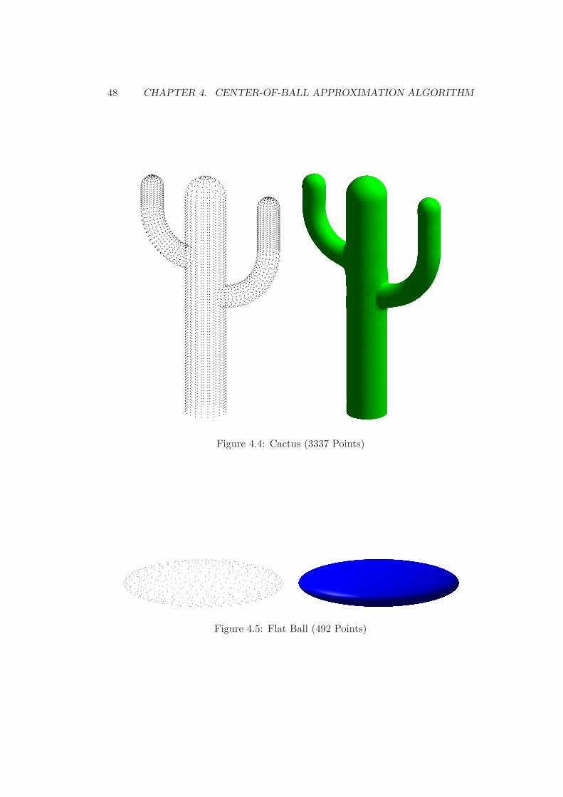
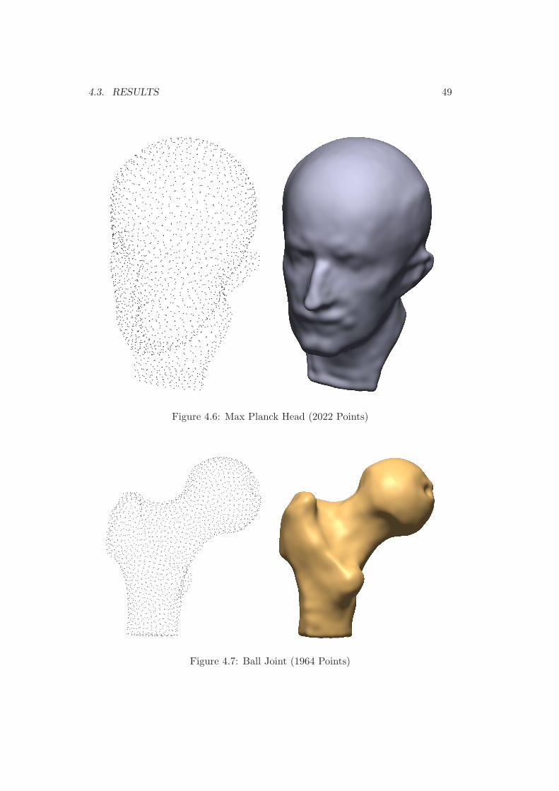
Figures 4.4 to 4.7 show some examples of shape reconstruction with the ZeroSlab-SVM using the algorithm introduced in the current chapter and a Gaussian kernel.As already mentioned in subsection 3.1.2, the kernel parameter σ should not bechosen too large in order to maintain a feasible numerical condition. Note that onethen has to find a good rendering strategy to visualize the level-set of the resultingfunction f defining the shape, since f will be more of a valley-type structure, whichcan impose some problems to standard rendering techniques for implicit surfacesas marching cubes. To address these problems, one can for example slightly de-crease the level-set value. However, changing the level-set value also reduces theinterpolation quality of the shape.


Figure 4.4: Cactus (3337 Points)

Figure 4.5: Flat Ball (492 Points)

4.3. RESULTS 49

Figure 4.6: Max Planck Head (2022 Points)

Figure 4.7: Ball Joint (1964 Points)

Chapter 5

Feature-Coefficient Correlation

5.1 Features of a Shape

In the context of pattern recognition, computer vision, medical imagery and free-form shape design, the work with features of a shape have become increasinglyimportant. The two features ridge and ravine are defined as local positive maximaof the maximal and local negative minima of the minimal principal curvature alongtheir associated principal curvature lines ([9],[10]). Ridges and ravines are deeplyconnected with interesting properties of a shape as its medial axis or its distancefunction.

5.2 Feature-Coefficient Correlation

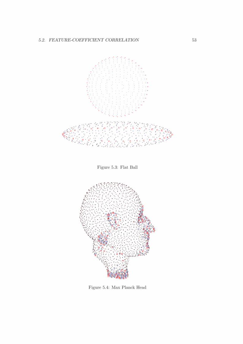
The observation was already made in [4] that features seem to correlate with thecoefficients (αi−α∗

i ) obtained from the solution of the SlabSVM using a Gaussiankernel. As we have seen in chapter 3 such a coefficient (αi−α∗

i ) is assigned to everysample point xi. The observation was that the coefficients with the highest valuesand the ones with negative values seem to correspond with ridges and ravines ofthe shape. This is shown in the figures 5.1-5.2, where the samples are color codedaccording to their corresponding coefficients.We now made the same observation for the ZeroSlabSVM. Figures 5.3-5.5 showsome examples, where the sample points are again color coded according to theirassociated coefficients αi, now stemming from the solution of the ZeroSlabSVM.

In figure 5.5 we can see that not only features as ridges, ravines or sharp edgesbut also the sampling density influences the values of those coefficients. A changeof sampling density on both arms of the cactus can for example produce negativecoefficients at points where no features exist.We know that the coefficients are the weights of a sum of Gaussians (see sub-section 3.1.2) which implicitly defines the reconstructed shape through one of itslevel-sets. It is therefore not difficult to gain some intuition on why the highest

51

52 CHAPTER 5. FEATURE-COEFFICIENT CORRELATION

Figure 5.1: Bunny

Figure 5.2: Rocker Arm

5.2. FEATURE-COEFFICIENT CORRELATION 53

Figure 5.3: Flat Ball

Figure 5.4: Max Planck Head

54 CHAPTER 5. FEATURE-COEFFICIENT CORRELATION

Figure 5.5: Cactus

and lowest coefficients will result at regions where the shape changes frequentlyor changes sharply. The coefficients will also automatically encode some localdensity information of the sample points, since the weighted sum must maintaina constant value on all sample points.An open task for future work would be to reach a better mathematical under-standing of these phenomena. However, such a mathematical investigation seemsto be quite involved. A good idea would probably be to first consider the specialcase of the ZeroSlabSVM, since it contains no open variables (as the slab size)and it approaches the shape reconstruction problem more directly. It would alsobe interesting to see whether the geometric insights gained so far could be usedto approach these challenging questions geometrically in the kernel induced highdimensional feature space.

Bibliography

[1] B. Scholkopf and A. Smola. Learning with Kernels: Support Vector Machines,Regularization, Optimization, and Beyond (Adaptive Computation and Ma-chine Learning). MIT Press, 2001.

[2] H. Wendland and R. Schaback. Kernel techniques: From machine learningto meshless methods. To appear in: Acta Numerica, 2006.

[3] B. Scholkopf, C. Burges, and V. Vapnik. Extracting support data for a giventask. In KDD, pages 252–257, 1995.

[4] S. Spalinger B. Scholkopf, J. Giesen. Kernel methods for implicit surfacemodeling. In NIPS, 2004.

[5] K. Fischer, B. Gartner, and M. Kutz. Fast smallest-enclosing-ball computa-tion in high dimensions. In Proceedings of the 11th Annual European Sympo-sium on Algorithms (ESA). Springer-Verlag, 2003.

[6] J. C. Carr, R. K. Beatson, J. B. Cherrie, T. J. Mitchell, W. R. Fright, B. C.McCallum, and T. R. Evans. Reconstruction and representation of 3D objectswith radial basis functions. In Eugene Fiume, editor, SIGGRAPH 2001, Com-puter Graphics Proceedings, pages 67–76. ACM Press / ACM SIGGRAPH,2001.

[7] H. Wendland. Scattered Data Approximation. Cambridge Monographs onApplied and Computational Mathematics. Cambridge University Press, 2005.

[8] T. Hastie, S. Rosset, R. Tibshirani, and J. Zhu. The entire regularizationpath for the support vector machine. Journal of Machine Learning Research,5:1391–1415, 2005.

[9] A. G. Belyaev, E. V. Anoshkina, and T. L. Kunii. Ridges, ravines and singu-larities. A. T. Fomenko and T. L. Kunii, Topological modeling for visualiza-tion, page Chapter 18, 1997.

[10] A. G. Belyaev, A. A. Pasko, and T. L. Kunii. Ridges and ravines on implicitsurfaces. In Proceedings of CGI’98, pages 530–535, 1998.

55

insights into the geometry of the gaussian kernel and an ... · the geometry of problems formulated...

Documents