1

Input Data Analysis: Specifying Model Parameters &

Distributions

Christos AlexopoulosDavid Goldsman

School of Industrial & Systems EngineeringGeorgia Tech

2

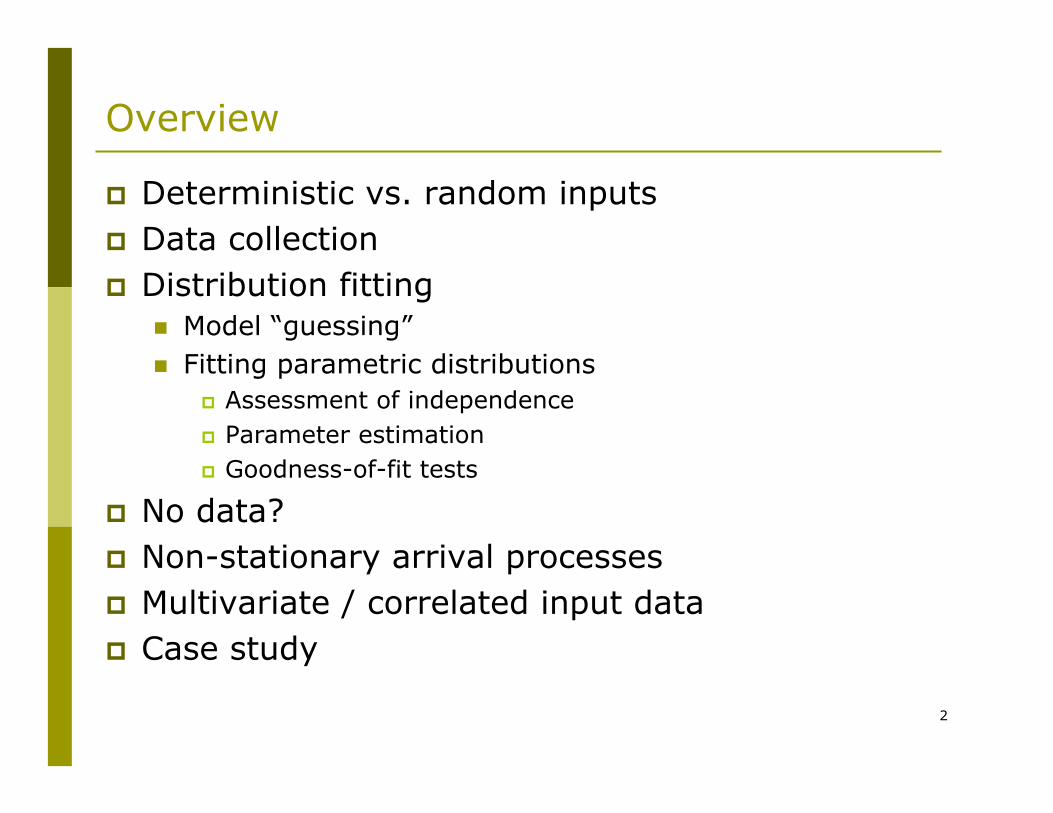
Overview

Deterministic vs. random inputsData collectionDistribution fitting

Model “guessing”Fitting parametric distributions

Assessment of independenceParameter estimationGoodness-of-fit tests

No data?Non-stationary arrival processesMultivariate / correlated input dataCase study

3

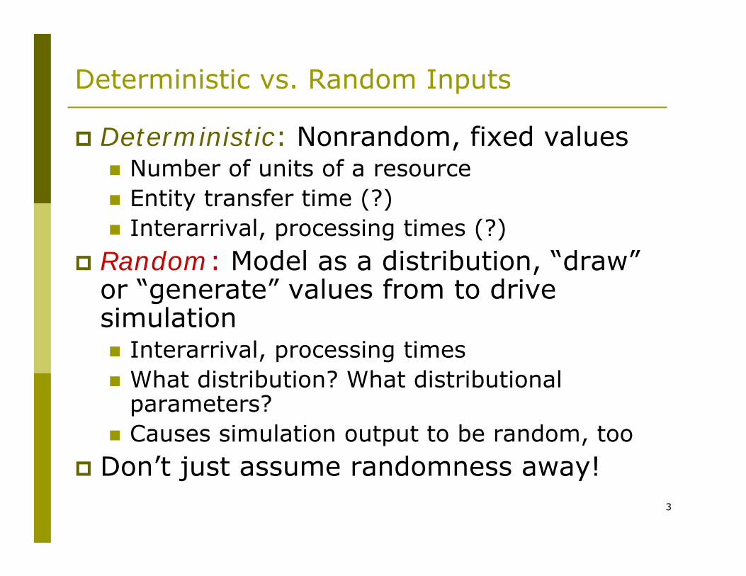
Deterministic vs. Random Inputs

Deterministic: Nonrandom, fixed valuesNumber of units of a resourceEntity transfer time (?)Interarrival, processing times (?)

Random: Model as a distribution, “draw”or “generate” values from to drive simulation

Interarrival, processing timesWhat distribution? What distributional parameters?Causes simulation output to be random, too

Don’t just assume randomness away!

4

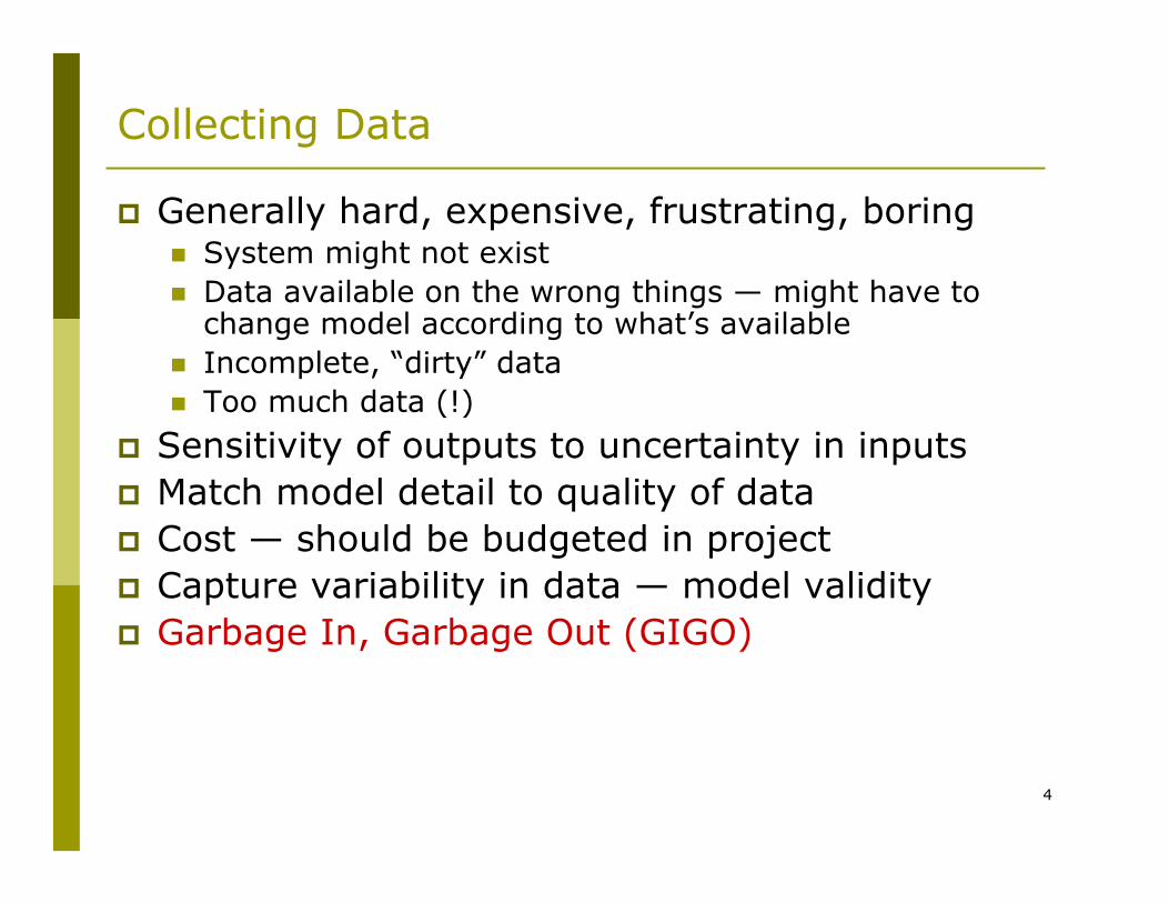
Collecting Data

Generally hard, expensive, frustrating, boringSystem might not existData available on the wrong things — might have to change model according to what’s availableIncomplete, “dirty” dataToo much data (!)

Sensitivity of outputs to uncertainty in inputsMatch model detail to quality of dataCost — should be budgeted in projectCapture variability in data — model validityGarbage In, Garbage Out (GIGO)

5

Using Data:Alternatives and Issues

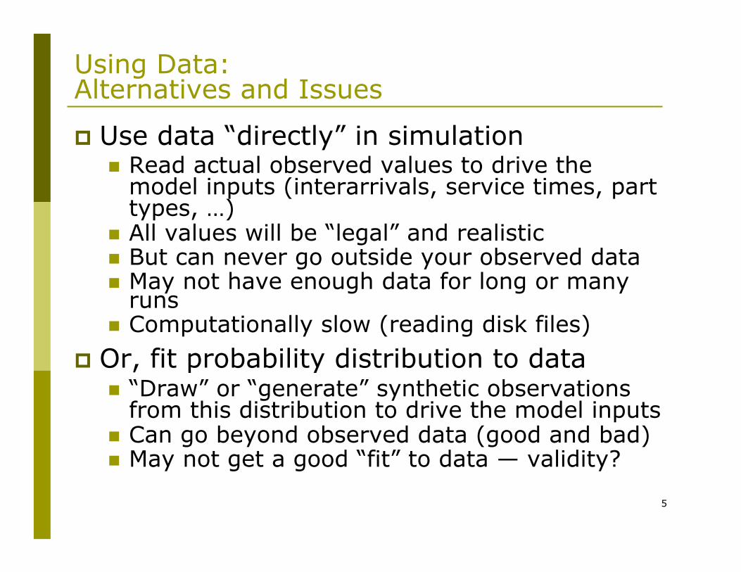
Use data “directly” in simulationRead actual observed values to drive the model inputs (interarrivals, service times, part types, …)All values will be “legal” and realisticBut can never go outside your observed dataMay not have enough data for long or many runsComputationally slow (reading disk files)

Or, fit probability distribution to data“Draw” or “generate” synthetic observations from this distribution to drive the model inputsCan go beyond observed data (good and bad)May not get a good “fit” to data — validity?

6

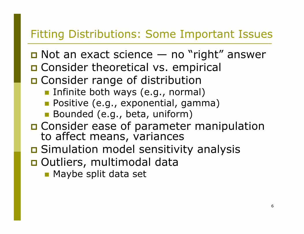
Fitting Distributions: Some Important Issues

Not an exact science — no “right” answerConsider theoretical vs. empiricalConsider range of distribution

Infinite both ways (e.g., normal)Positive (e.g., exponential, gamma)Bounded (e.g., beta, uniform)

Consider ease of parameter manipulation to affect means, variancesSimulation model sensitivity analysisOutliers, multimodal data

Maybe split data set

7

Main Steps (continued)

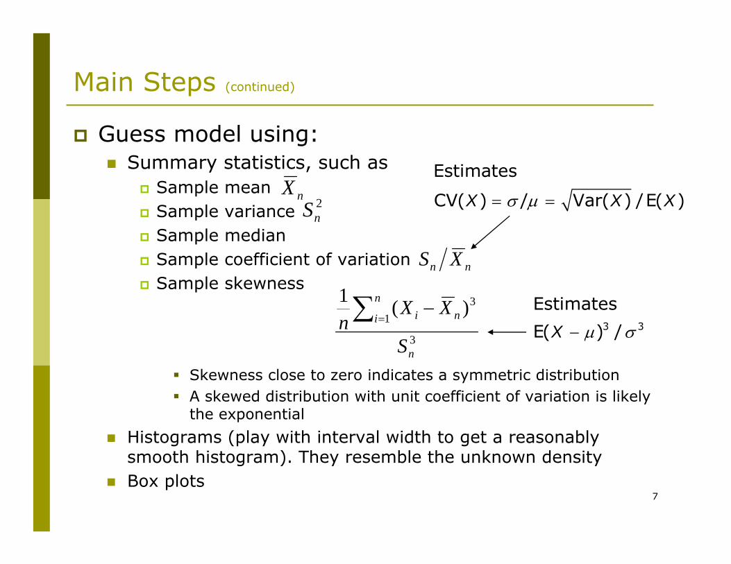
Guess model using:Summary statistics, such as

Sample meanSample varianceSample medianSample coefficient of variationSample skewness

Skewness close to zero indicates a symmetric distributionA skewed distribution with unit coefficient of variation is likely the exponential

Histograms (play with interval width to get a reasonably smooth histogram). They resemble the unknown densityBox plots

nX2nS

nn XS

3

13)(1

n

n

i ni

S

XXn ∑ =

−

Estimates

CV( ) / Var( ) /E( )X X Xσ µ= =

3 3

Estimates

E( ) /X µ σ−

8

Main Steps (continued)

If a parametric models seems plausible:Estimate parametersTest goodness-of-fit

9

Fitting Parametric Distributions

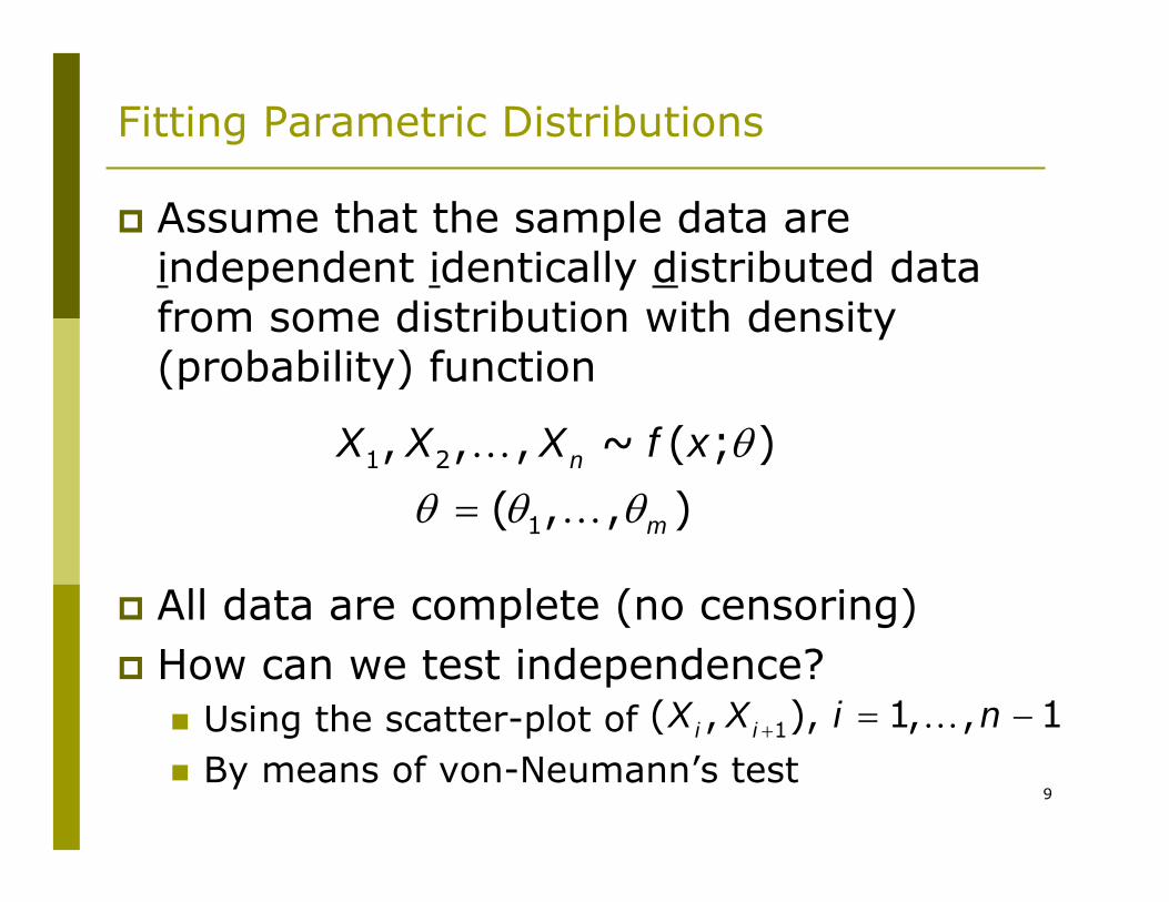
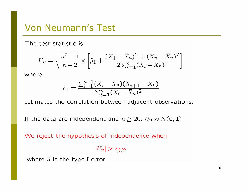
Assume that the sample data are independent identically distributed data from some distribution with density (probability) function

All data are complete (no censoring)How can we test independence?

Using the scatter-plot of By means of von-Neumann’s test

θθ θ θ=

K

K

1 2

1

, , , ~ ( ; )

( , , )n

m

X X X f x

+ = −K1( , ), 1, , 1i iX X i n

10

Von Neumann’s Test

11

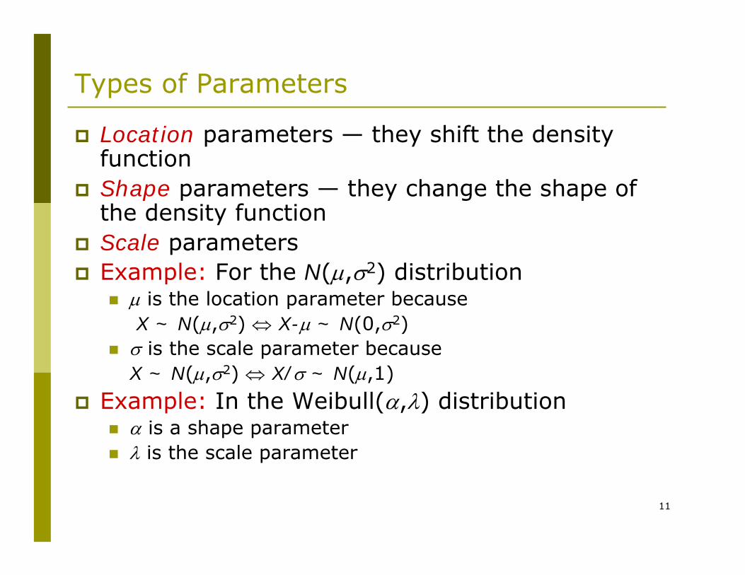
Types of Parameters

Location parameters — they shift the density functionShape parameters — they change the shape of the density functionScale parametersExample: For the N(µ,σ2) distribution

µ is the location parameter becauseX ~ N(µ,σ2) ⇔ X-µ ~ N(0,σ2)

σ is the scale parameter becauseX ~ N(µ,σ2) ⇔ X/σ ~ N(µ,1)

Example: In the Weibull(α,λ) distributionα is a shape parameterλ is the scale parameter

12

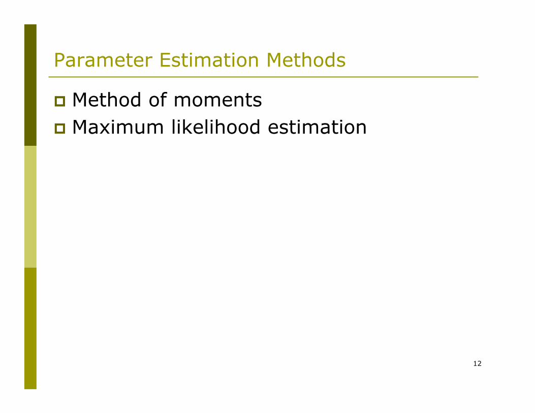
Parameter Estimation Methods

Method of momentsMaximum likelihood estimation

13

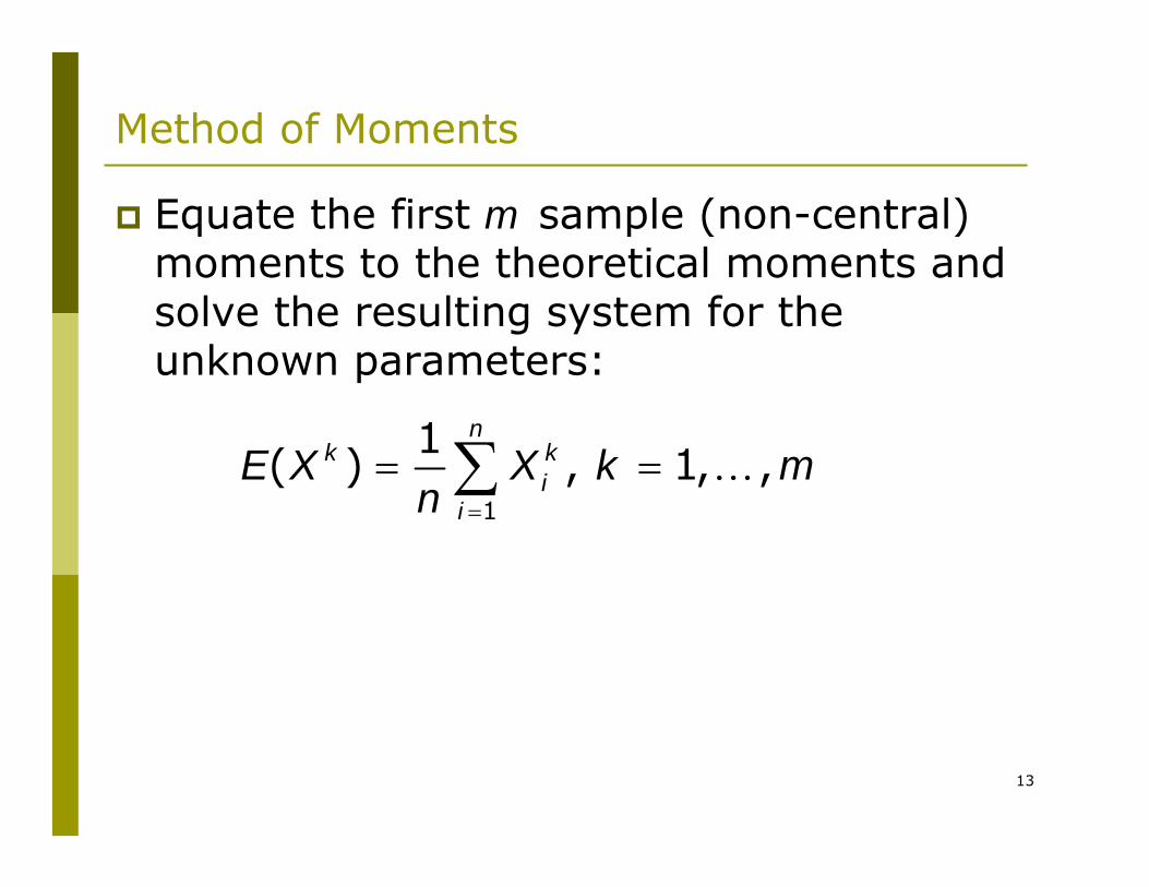
Method of Moments

Equate the first m sample (non-central) moments to the theoretical moments and solve the resulting system for the unknown parameters:

=

= =∑ K1

1( ) , 1, ,

nk k

ii

E X X k mn

14

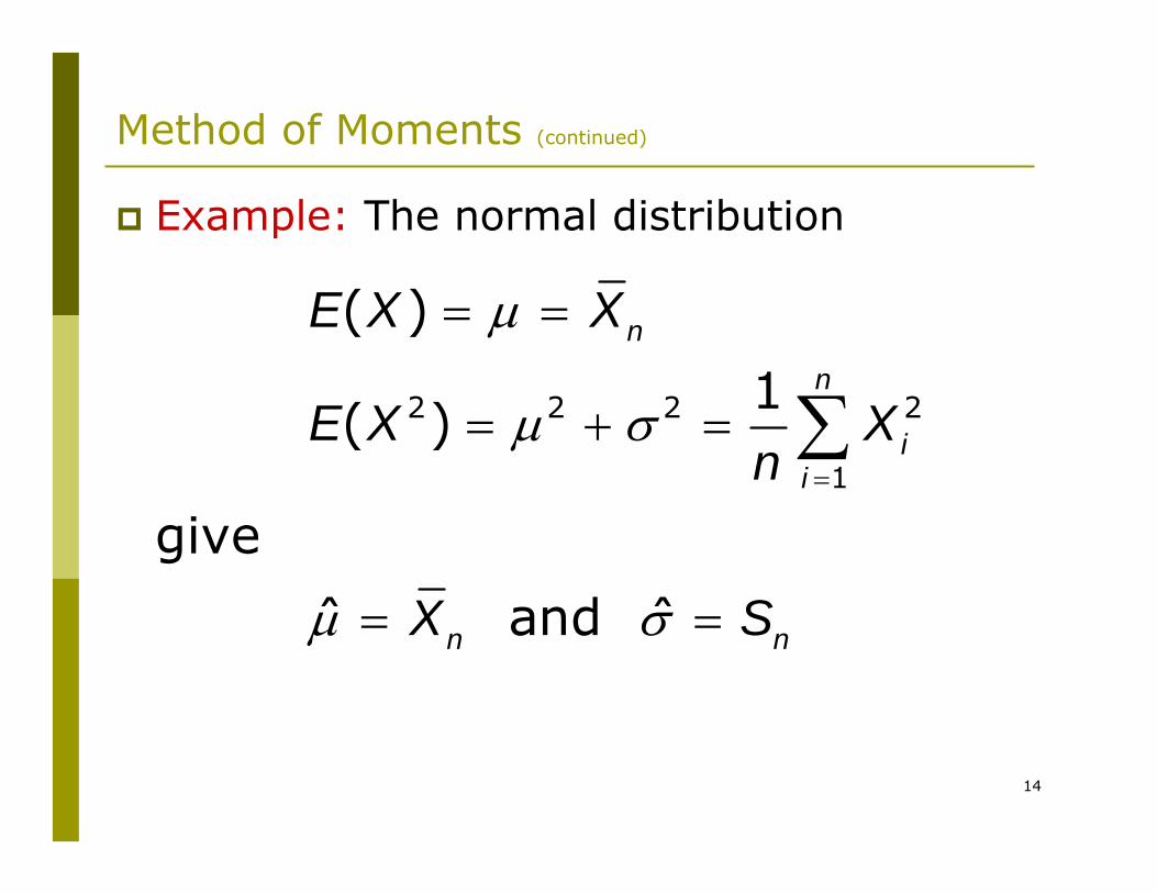
Method of Moments (continued)

Example: The normal distribution

µ

µ σ

µ σ

=

= =

= + =

= =

∑2 2 2 2

1

( )

1( )

give

and ˆ ˆ

n

n

ii

n n

E X X

E X Xn

X S

15

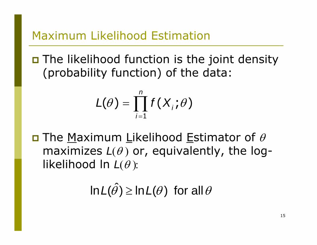
Maximum Likelihood Estimation

The likelihood function is the joint density (probability function) of the data:

The Maximum Likelihood Estimator of θmaximizes L(θ ) or, equivalently, the log-likelihood ln L(θ ):

θ θ=

= ∏1

( ) ( ; )n

ii

L f X

θθθ all for )(ln)ˆ(ln LL ≥

16

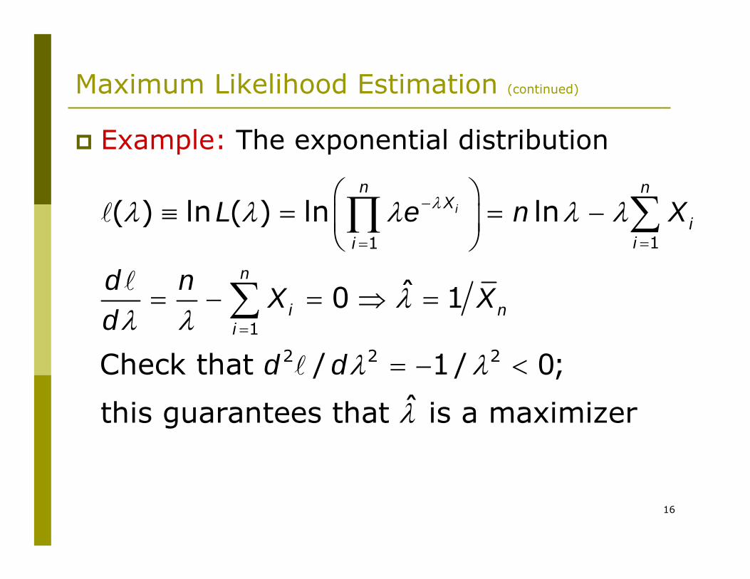
Maximum Likelihood Estimation (continued)

Example: The exponential distribution

λλ λ λ λ λ

λλ λ

λ λ

λ

−

==

=

⎛ ⎞≡ = = −⎜ ⎟

⎝ ⎠

= − = ⇒ =

= − <

∑∏

∑

l

l

l

11

1

2 2 2

( ) ln ( ) ln ln

ˆ0 1

Check that / 1 / 0;

ˆthis guarantees that is a maximizer

i

n nX

iii

n

i ni

L e n X

d nX X

d

d d

17

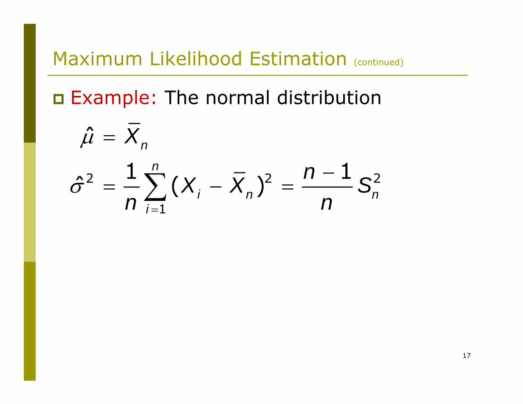
Maximum Likelihood Estimation (continued)

Example: The normal distribution

µ

σ=

=

−= − =∑2 2 2

1

ˆ

1 1( )ˆ

n

n

i n ni

X

nX X S

n n

18

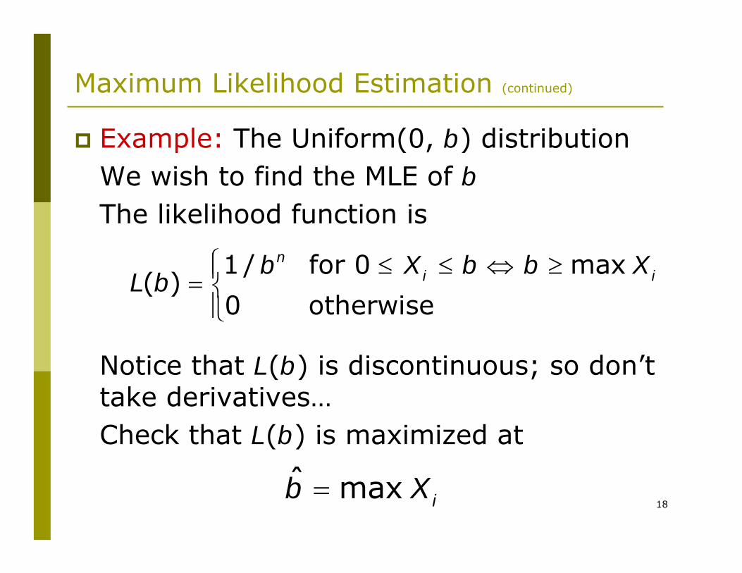
Maximum Likelihood Estimation (continued)

Example: The Uniform(0, b) distributionWe wish to find the MLE of bThe likelihood function is

Notice that L(b) is discontinuous; so don’t take derivatives…Check that L(b) is maximized at

1 / for 0 max( )

0 otherwise

ni ib X b b X

L b⎧ ≤ ≤ ⇔ ≥⎪= ⎨⎪⎩

ˆ max ib X=

19

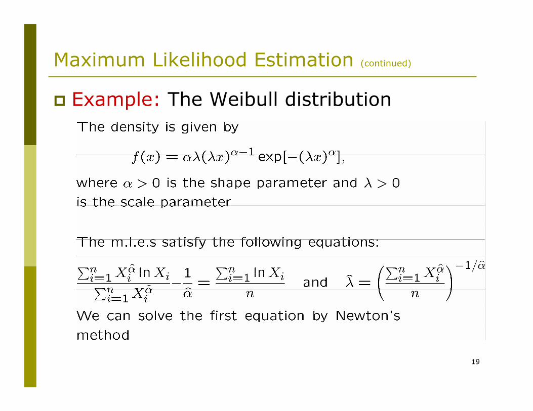
Maximum Likelihood Estimation (continued)

Example: The Weibull distribution

20

Maximum Likelihood Estimation (continued)

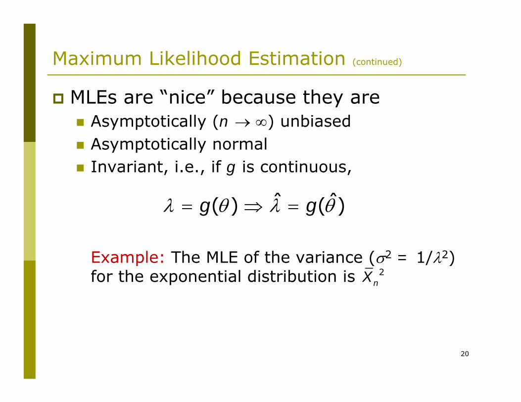
MLEs are “nice” because they areAsymptotically (n → ∞) unbiasedAsymptotically normalInvariant, i.e., if g is continuous,

Example: The MLE of the variance (σ2 = 1/λ2)for the exponential distribution is

λ θ λ θ= ⇒ =ˆ ˆ( ) ( )g g

2nX

21

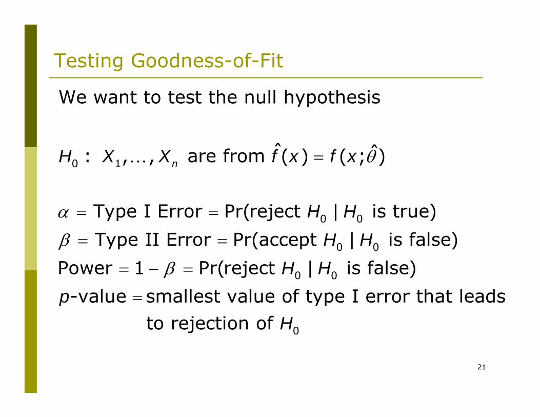
Testing Goodness-of-Fit

θ

αβ

β

=

= =

= =

= − =

=

K0 1

0 0

0 0

0 0

We want to test the null hypothesis

ˆ ˆ: , , are from ( ) ( ; )

Type I Error Pr(reject | is true)

Type II Error Pr(accept | is false)

Power 1 Pr(reject | is false)

-value smallest

nH X X f x f x

H H

H H

H H

p

0

value of type I error that leads to rejection of H

22

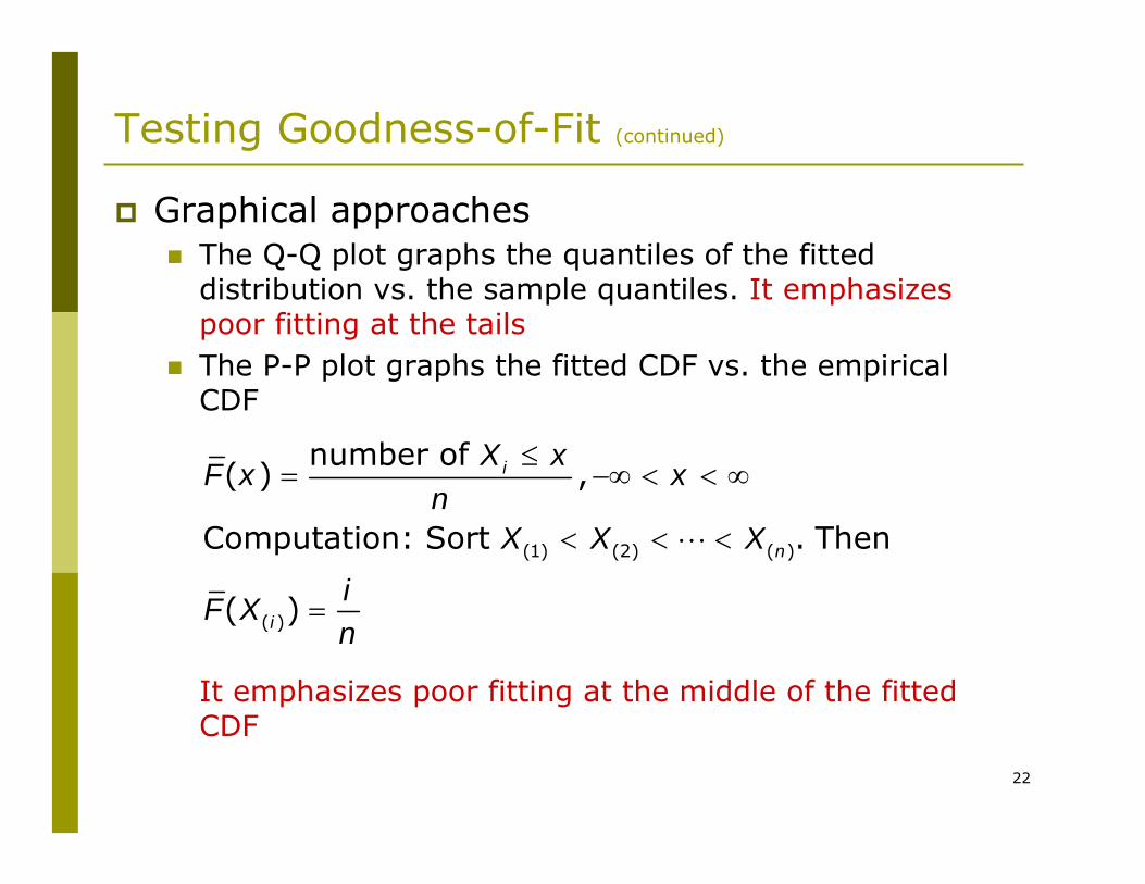
Testing Goodness-of-Fit (continued)

Graphical approachesThe Q-Q plot graphs the quantiles of the fitted distribution vs. the sample quantiles. It emphasizes poor fitting at the tailsThe P-P plot graphs the fitted CDF vs. the empirical CDF

It emphasizes poor fitting at the middle of the fitted CDF

≤= −∞ < < ∞

< < <

=

L(1) (2) ( )

( )

number of ( ) ,

Computation: Sort . Then

( )

i

n

i

X xF x x

nX X X

iF X

n

23

Testing Goodness-of-Fit (continued)

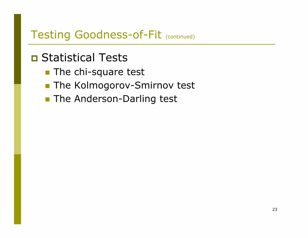
Statistical TestsThe chi-square testThe Kolmogorov-Smirnov testThe Anderson-Darling test

24

The Chi-square Test

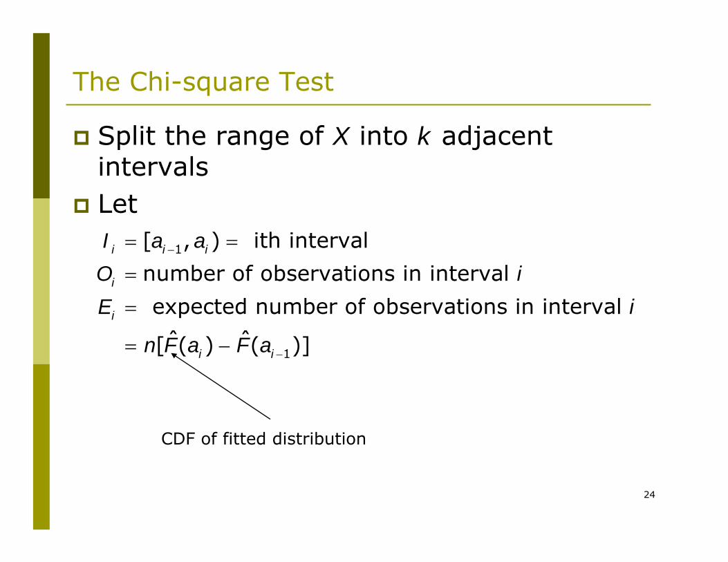
Split the range of X into k adjacent intervalsLet

1

1

[ , ) ith interval

number of observations in interval

expected number of observations in interval

ˆ ˆ[ ( ) ( )]

i i i

i

i

i i

I a a

O i

E i

n F a F a

−

−

= =

=

=

= −

CDF of fitted distribution

25

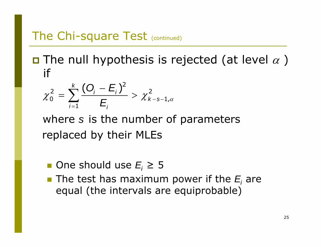
The Chi-square Test (continued)

The null hypothesis is rejected (at level α ) if

One should use Ei ≥ 5The test has maximum power if the Ei are equal (the intervals are equiprobable)

αχ χ − −=

−= >∑

22 20 1,

1

( )

where is the number of parameters replaced by their MLEs

ki i

k si i

O EE

s

26

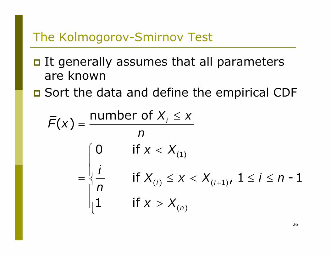
The Kolmogorov-Smirnov Test

It generally assumes that all parameters are knownSort the data and define the empirical CDF

+

≤=

<⎧⎪⎪= ≤ < ≤ ≤⎨⎪

>⎪⎩

(1)

( ) ( 1)

( )

number of ( )

0 if

if , 1 -1

1 if

i

i i

n

X xF x

nx X

iX x X i n

nx X

27

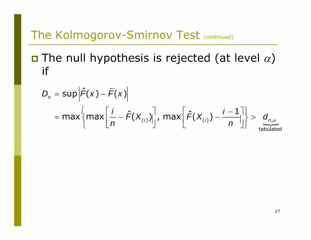
The Kolmogorov-Smirnov Test (continued)

The null hypothesis is rejected (at level α) if

{( ) ( ) ,

tabulated

ˆsup ( ) ( )

1ˆ ˆmax max ( ) , max ( )

n

i i n

D F x F x

i iF X F X d

n n α

= −

⎧ ⎫−⎡ ⎤ ⎡ ⎤= − − >⎨ ⎬⎢ ⎥ ⎢ ⎥⎣ ⎦ ⎣ ⎦⎩ ⎭

28

The Kolmogorov-Smirnov Test (continued)

We usually simplify the above inequality by computing a modified test statistic and a modified critical value :

When parameters are replaced by MLEs modified K-S test statistics exist for the following distributions:

NormalExponentialWeibullLog-logistic

{α>tabulated

Adjusted Test Statistic c

αc

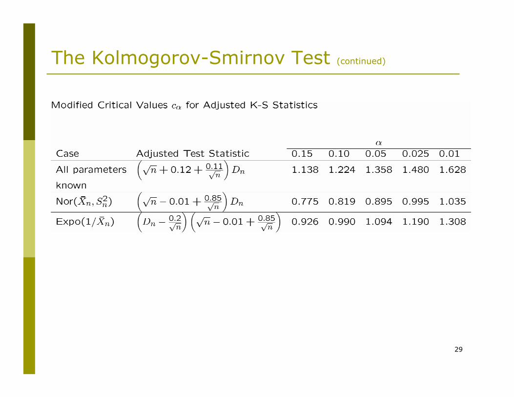
29

The Kolmogorov-Smirnov Test (continued)

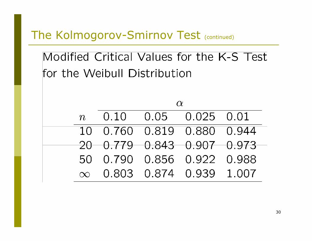
30

The Kolmogorov-Smirnov Test (continued)

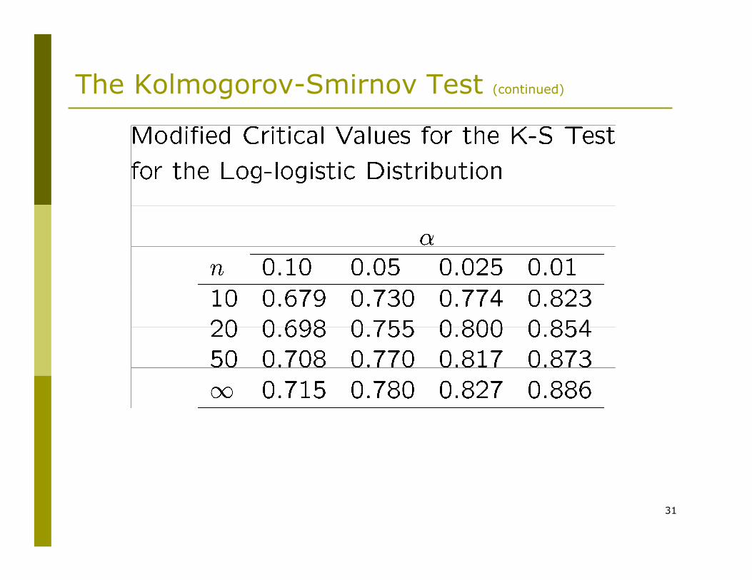
31

The Kolmogorov-Smirnov Test (continued)

32

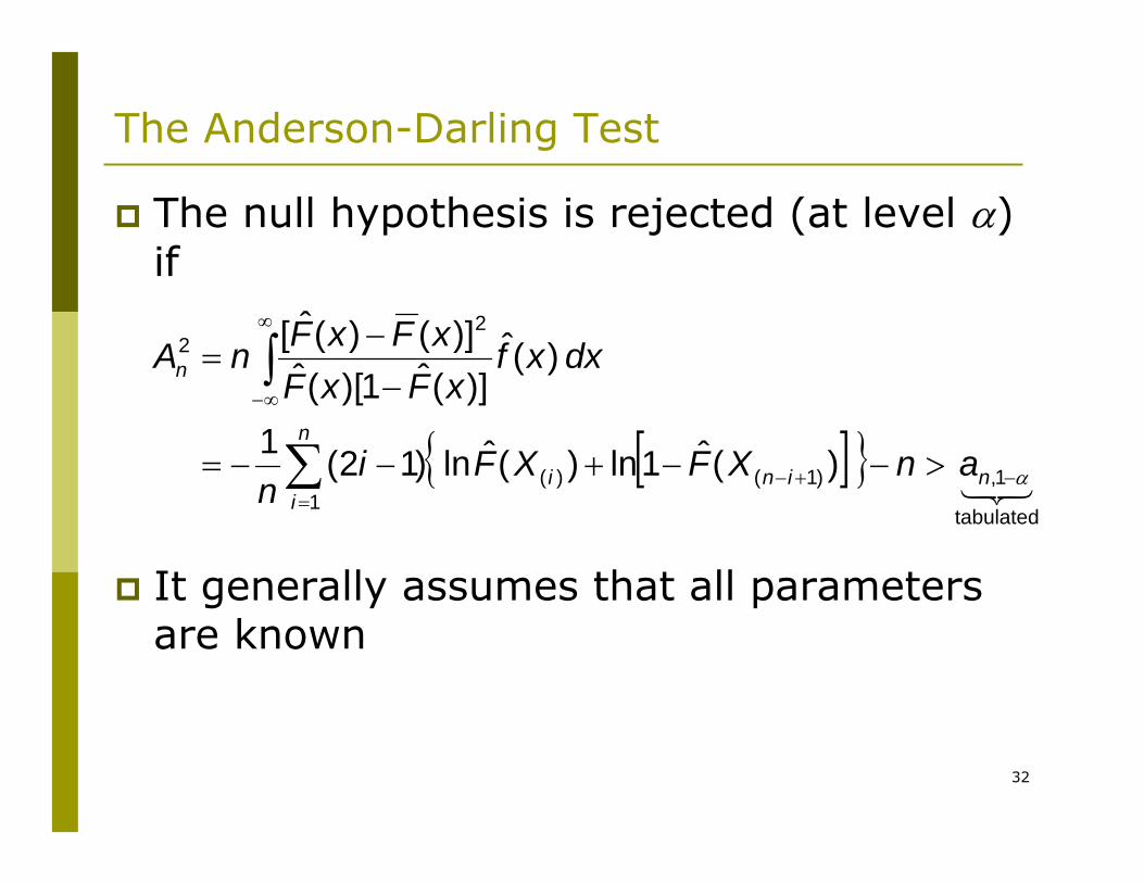
The Anderson-Darling Test

The null hypothesis is rejected (at level α) if

It generally assumes that all parameters are known

[ ]{ }∑

∫

=−+−

∞

∞−

>−−+−−=

−−

=

n

inini

n

anXFXFin

dxxfxFxF

xFxFnA

1tabulated

1,)1()(

22

)(ˆ1ln)(ˆln )12(1

)(ˆ)](ˆ1)[(ˆ

)]()(ˆ[

321 α

33

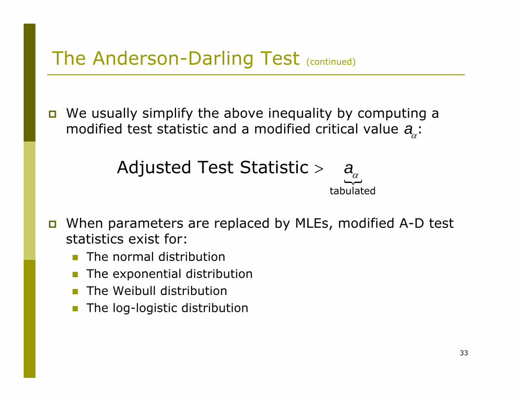
The Anderson-Darling Test (continued)

We usually simplify the above inequality by computing a modified test statistic and a modified critical value :

When parameters are replaced by MLEs, modified A-D test statistics exist for:

The normal distributionThe exponential distributionThe Weibull distributionThe log-logistic distribution

αa

{α>tabulated

Adjusted Test Statistic a

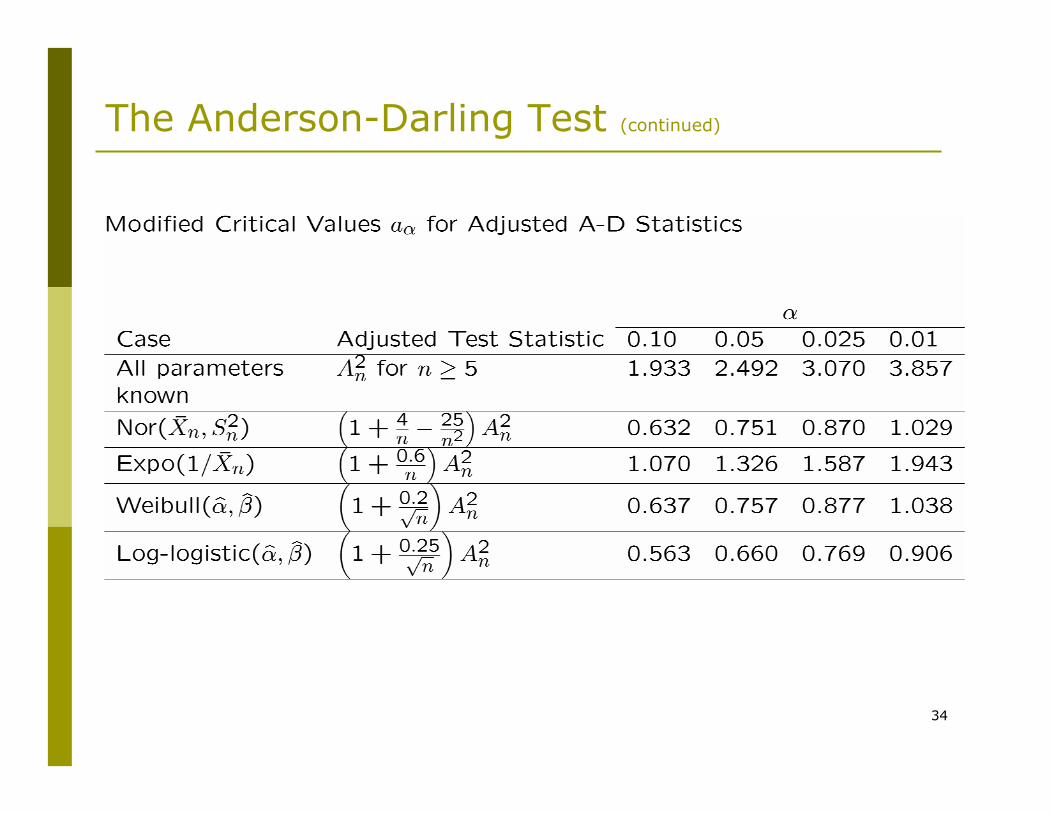
34

The Anderson-Darling Test (continued)

35

No Data?

Happens more often than you would likeNo good solution; some (bad) options:

Interview “experts”Min, Max: UniformAverage, % error or absolute error: UniformMin, Mode, Max: Triangular

Mode can be different from Mean — allows asymmetry (skewness)

Interarrivals — independent, stationaryExponential — still need some value for mean

Number of “random” events in an interval: PoissonSum of independent “pieces”: normalProduct of independent “pieces”: lognormal

36

Non-stationary Arrival Processes

External events (often arrivals) whose rate varies over time

Lunchtime at fast-food restaurantsRush-hour traffic in citiesTelephone call centersSeasonal demands for a manufactured product

It can be critical to model this non-stationarity for model validity

Ignoring peaks, valleys can mask important behaviorCan miss rush hours, etc.

Good model: Non-stationary Poisson process

37

Non-stationary Arrival Processes (continued)

Two issues:How to specify/estimate the rate functionHow to generate from it properly during the simulation (will be discussed during the Output Analysis session)

Several ways to estimate rate function — we’ll just do the piecewise-constant method

Divide time frame of simulation into subintervals of time over which you think rate is fairly flatCompute observed rate within each subintervalBe very careful about time units!

Model time units = minutesSubintervals = half hour (= 30 minutes)45 arrivals in the half hour; rate = 45/30 = 1.5 per minute

38

Multivariate and Correlated Input Data

Usually we assume that all generated random observations across a simulation are independent (though from possibly different distributions)Sometimes this isn’t true:

A “difficult” part may require longer service times by a set of machinesThis indicates positive correlation

Ignoring such relations can invalidate model

39

Case Study: Times-to-Failure

A data set contains 200 times-to-failure for a piece of equipmentWe use ExpertFit®

To assess independence, we create a scatter plot

40

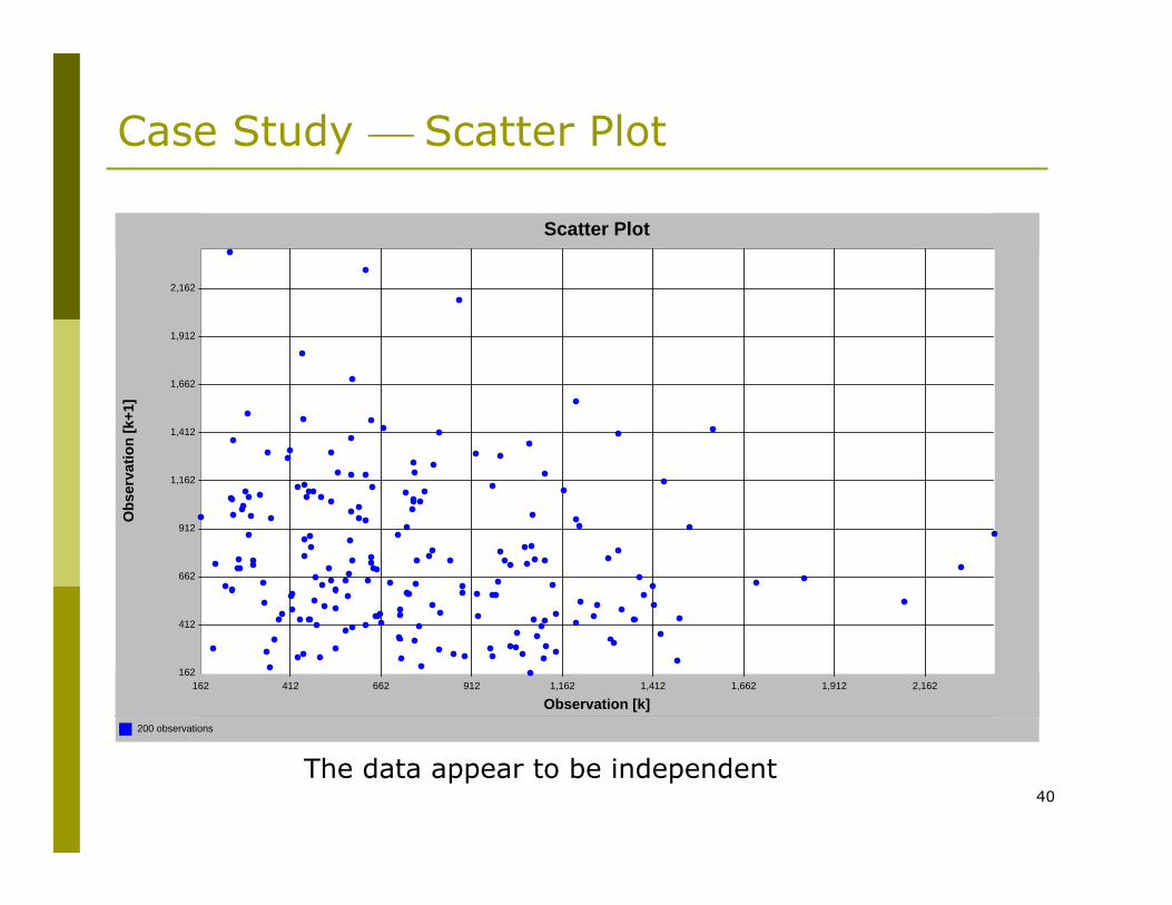
Case Study ⎯ Scatter Plot

200 observations

162 412 662 912 1,162 1,412 1,662 1,912 2,162162

412

662

912

1,162

1,412

1,662

1,912

2,162

Scatter Plot

Observation [k]

Obs

erva

tion

[k+1

]

The data appear to be independent

41

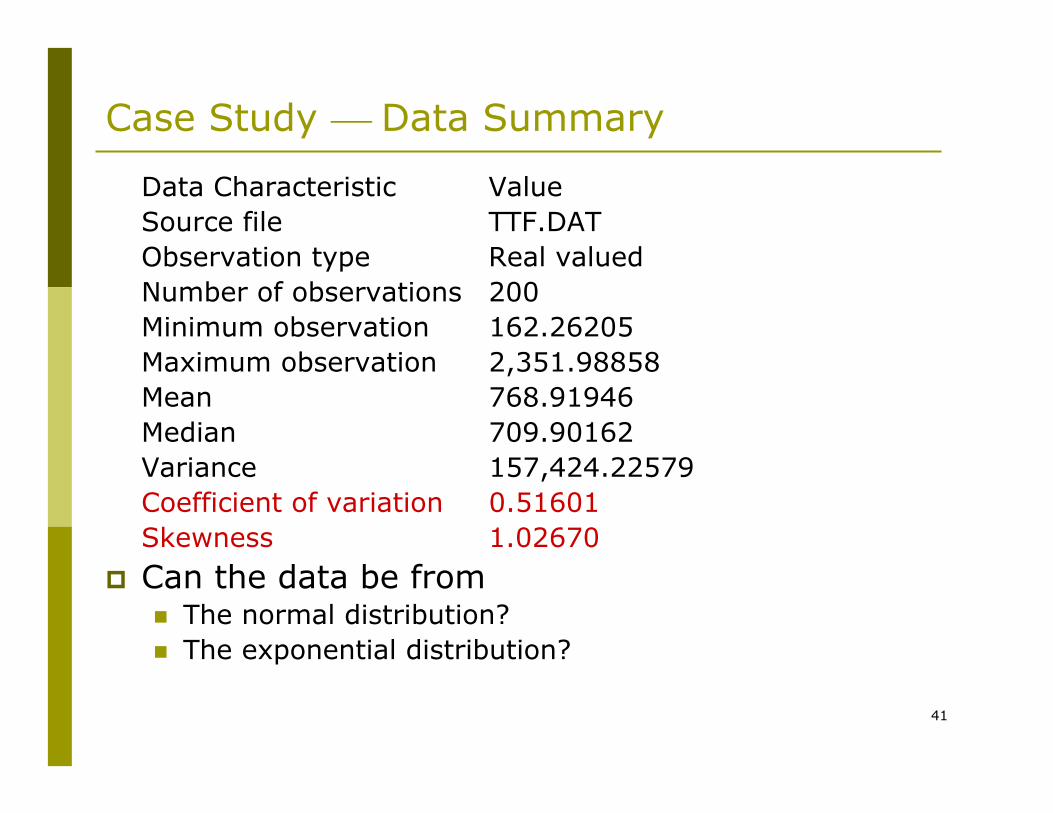
Case Study ⎯ Data Summary

Data Characteristic ValueSource file TTF.DATObservation type Real valuedNumber of observations 200Minimum observation 162.26205Maximum observation 2,351.98858Mean 768.91946Median 709.90162Variance 157,424.22579Coefficient of variation 0.51601Skewness 1.02670

Can the data be fromThe normal distribution?The exponential distribution?

42

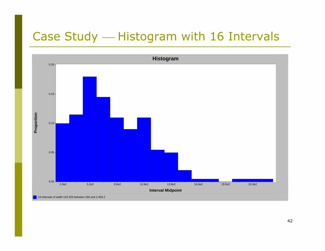
Case Study ⎯ Histogram with 16 Intervals

16 intervals of width 143.325 between 160 and 2,453.2

0.00

0.05

0.10

0.15

0.20

Histogram

Interval Midpoint

Prop

ortio

n

2.3e2 5.2e2 8.0e2 10.9e2 13.8e2 16.6e2 19.5e2 22.4e2

43

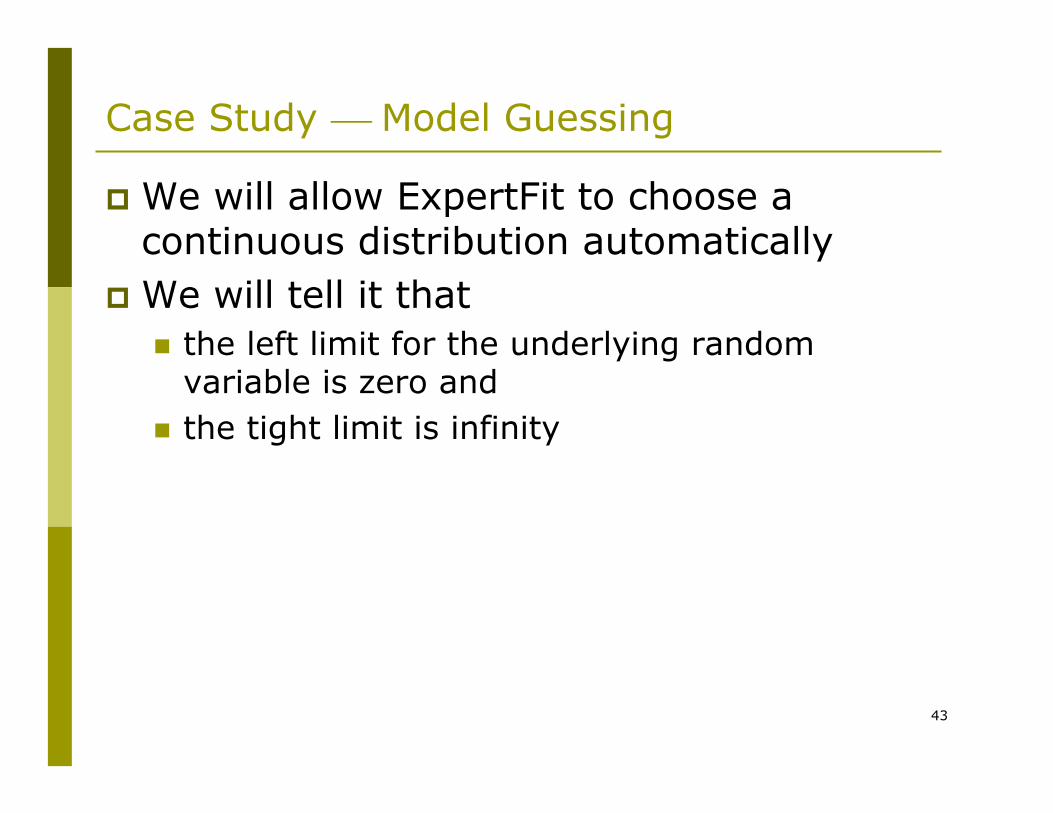
Case Study ⎯ Model Guessing

We will allow ExpertFit to choose a continuous distribution automaticallyWe will tell it that

the left limit for the underlying random variable is zero andthe tight limit is infinity

44

Case Study ⎯ ExpertFit’s Choice…

Weibull(E): Weibulldistribution with a location parameter

45

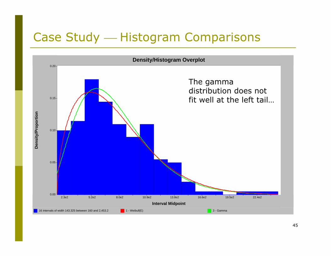
Case Study ⎯ Histogram Comparisons

16 intervals of width 143.325 between 160 and 2,453.2 1 - Weibull(E) 3 - Gamma

0.00

0.05

0.10

0.15

0.20

Density/Histogram Overplot

Interval Midpoint

Den

sity

/Pro

port

ion

2.3e2 5.2e2 8.0e2 10.9e2 13.8e2 16.6e2 19.5e2 22.4e2

The gamma distribution does not fit well at the left tail…

46

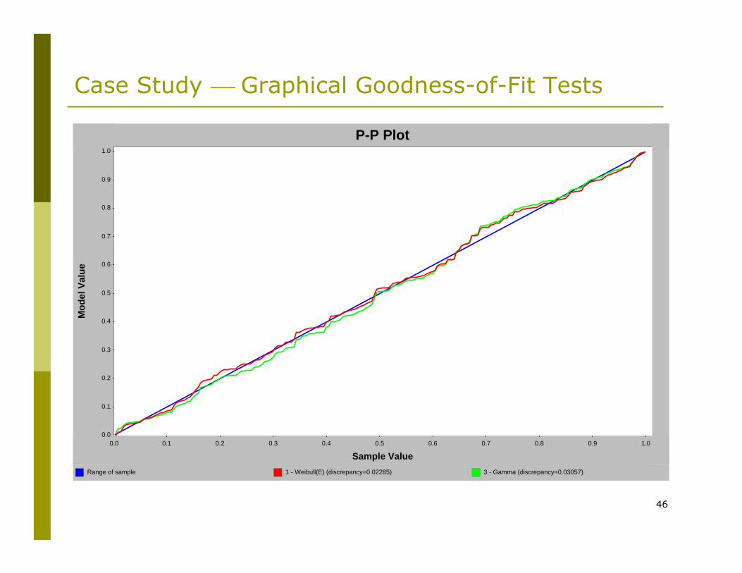
Case Study ⎯ Graphical Goodness-of-Fit Tests

Range of sample 1 - Weibull(E) (discrepancy=0.02285) 3 - Gamma (discrepancy=0.03057)

0.0 0.1 0.2 0.3 0.4 0.5 0.6 0.7 0.8 0.9 1.00.0

0.1

0.2

0.3

0.4

0.5

0.6

0.7

0.8

0.9

1.0

P-P Plot

Sample Value

Mod

el V

alue

47

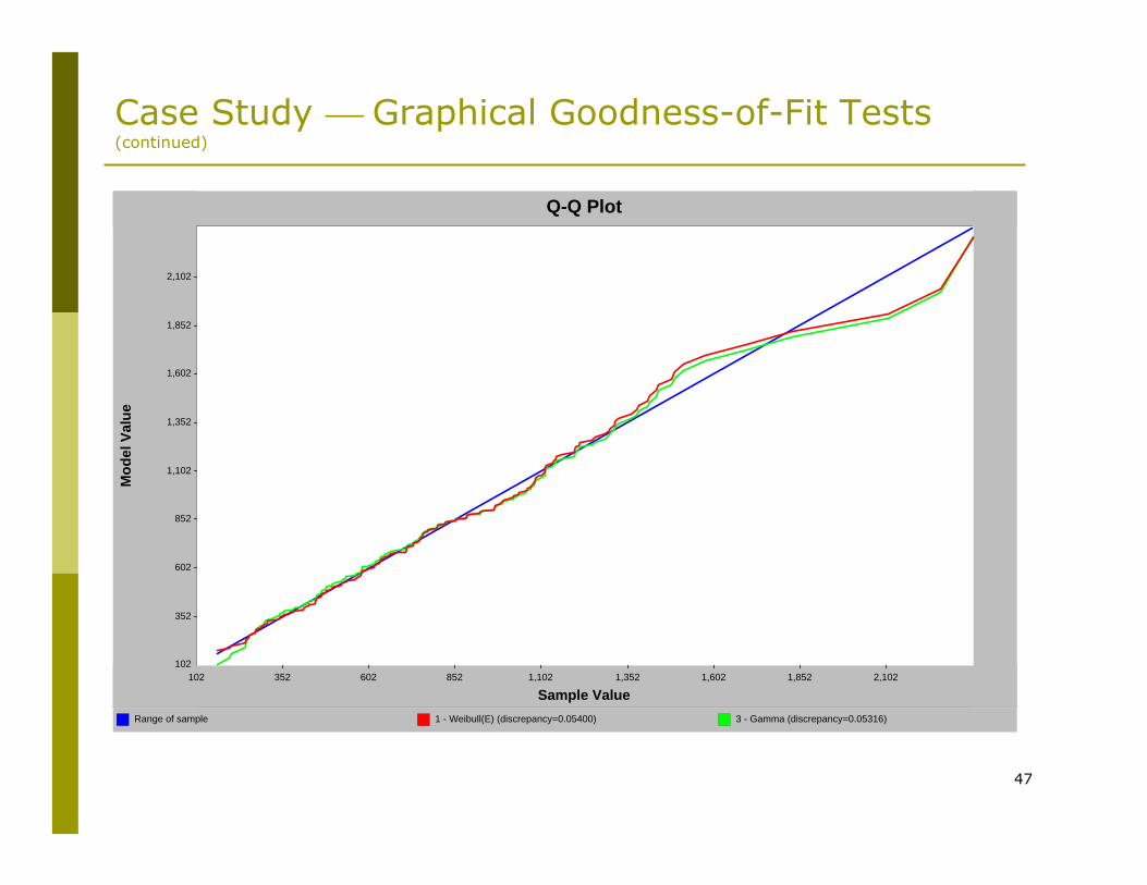
Case Study ⎯ Graphical Goodness-of-Fit Tests (continued)

Range of sample 1 - Weibull(E) (discrepancy=0.05400) 3 - Gamma (discrepancy=0.05316)

102 352 602 852 1,102 1,352 1,602 1,852 2,102102

352

602

852

1,102

1,352

1,602

1,852

2,102

Q-Q Plot

Sample Value

Mod

el V

alue

48

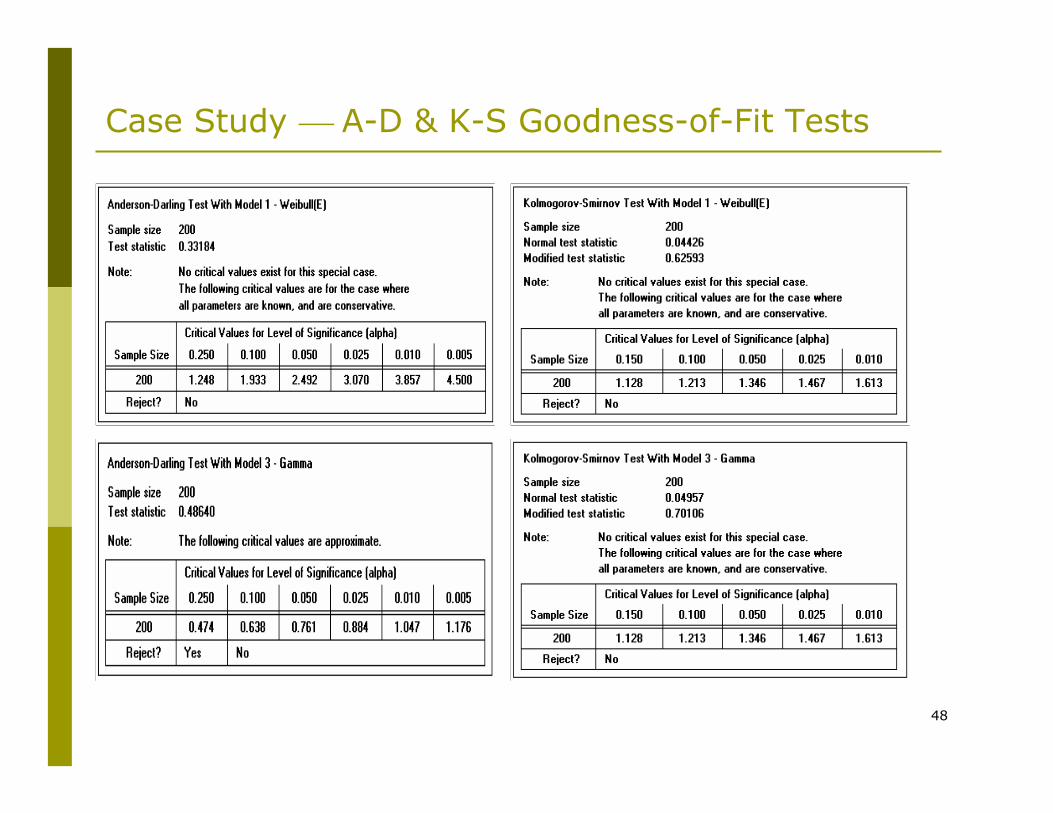
Case Study ⎯ A-D & K-S Goodness-of-Fit Tests

49

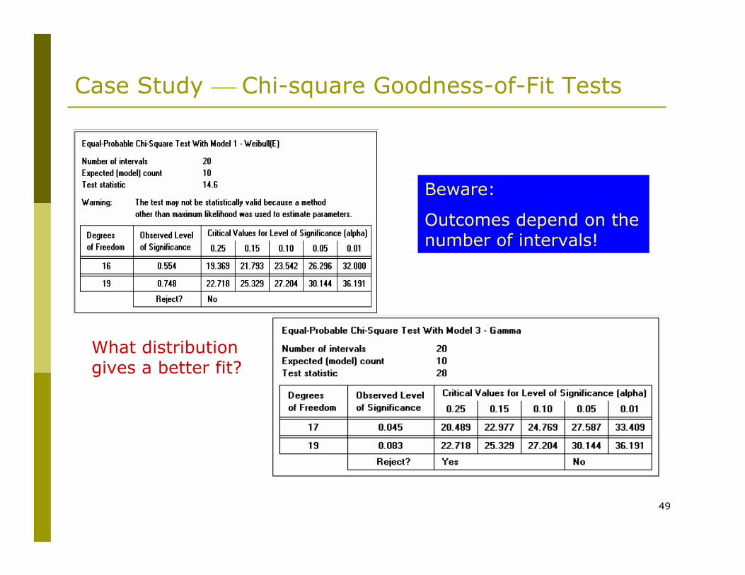
Case Study ⎯ Chi-square Goodness-of-Fit Tests

What distribution gives a better fit?

Beware:

Outcomes depend on the number of intervals!

50

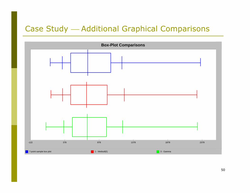
Case Study ⎯ Additional Graphical Comparisons

7-point sample box plot 1 - Weibull(E) 3 - Gamma

-122 378 878 1378 1878 2378

Box-Plot Comparisons

51

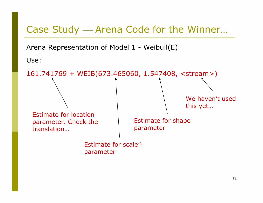
Case Study ⎯ Arena Code for the Winner…

Arena Representation of Model 1 - Weibull(E)

Use:

161.741769 + WEIB(673.465060, 1.547408, <stream>)

Estimate for location parameter. Check the translation…

Estimate for scale-1

parameter

Estimate for shape parameter

We haven’t used this yet…