Department of Engineering Physicsand Mathematics

Tero Tuominen

Information Model of an Electricity Procurement Plan-ning System

Master’s thesis submitted in partial fulfillment of the requirements for thedegree of Master of Science in Technology

Helsinki, December 2005

Supervisor: Professor Ahti SaloInstructor: M.Sc. Otso Ojanen

ii

HELSINKI UNIVERSITY OF TECHNOLOGY ABSTRACT OF MASTER’S THESISAuthor: Tero TuominenDepartment: Department of Engineering Physics and MathematicsMajor subject: Systems Analysis and Operations ResearchMinor subject: Corporate Strategy and International BusinessTitle: Information Model of Electricity Procurement

Planning SystemChair: Mat-2 Applied MathematicsSupervisor: Professor Ahti SaloInstructor: M.Sc. Otso Ojanen

Balance responsible (BR) is the player on rather turbulent deregulated energy markets whocarries a financial responsibility of the physical energy balance within his balance area. Main-taining the balance between generation and consumption — procurement and delivery obliga-tions — is further complicated by combined heat and power generation. In rapidly changingmarkets BR thus faces an optimization problem whose difficulty arises from two sources: first,the technicalities of the optimization itself and secondly, the management of the informationfrom multiple independent sources. The latter one is of interest in this thesis.

This thesis has two-fold objectives: first, to develop an extensive energy procurement modelfor BR, and secondly, to create a structured representation of the prerequisite information thatthe optimization algorithms need in order to be able to provide the decision support for BR.The underlying decision support system is assumed to be structured so that the system andthe actual optimization algorithms are separated and the supported algorithms are not fixedbeforehand. The treatment is thus algorithm-independent.

The aim of the first task is to lay down the basis both for the simulation model to be laterused e.g. for verification purposes and to identify the information needs of the optimizationalgorithms. The level of detail of the model is to largely set by the simulation needs; theresulting model is inevitably far too complex to be optimized as such. The actual modeling isbased both on the component models found in the literature and author’s own choices. Specialattention is paid to the hydropower system model. The information needs of the system, onthe other hand, are set based on the same mathematical model taking care that all the relevantinformation is incorporated irrespective of the chosen algorithms.

The information modeling aims to lay down the foundation for structuring the algorithm-independent information so that its rendering into an interface file between the computer ap-plications is straightforward. Thus the ultimate aim of the information modeling is to providea common access to the algorithm-independent information relevant to the BR’s procurementplanning in a standardized manner. Generally the information modeling begins by creating anontology on the domain and identifying the relationships between the entities. In this case thestarting point is the mathematical model and the task is thus rather exceptional from the in-formation modeling point of view. Beginning from mathematical model both the ontology andrelationships turn out to be quite readily available and the task proceeds straightforwardly intoconceptual schemas of the model components.

N. of pages: viii+75 Keywords: energy procurement, information modelingDepartment fillsApproved: Library code:

iii

TEKNILLINEN KORKEAKOULU DIPLOMITYÖN TIIVISTELMÄTekijä: Tero TuominenOsasto: Teknillisen fysiikan ja matematiikan osastoPääaine: Systeemi- ja operaatiotutkimusSivuaine: Yritysstrategia ja kansainvälinen liiketoimintaTyön nimi: Sähkönhankinnan tukijärjestelmän tietomalliProfessuuri: Mat-2 Sovellettu matematiikkaValvoja: Professori Ahti SaloOhjaaja: DI, KTM Otso Ojanen

Tasevastaava (TV) toimii sangen turbulenteilla vapautuneilla energiamarkkinoilla, ja kantaataloudellisen vastuun oman tasealueensa fyysisestä energiataseesta. Kulutuksen ja tuotannon— hankinnan ja toimitusvelvoitteiden — välisen tasapainon ylläpitämistä vaikeuttaa edelleenyhdistetty sähkön ja lämmöntuotanto. Nopeasti muuttuvilla markkinoilla TV kohtaa täten op-timointiongelman, jonka vaikeus on peräisin kahdesta lähteestä: toisaalta itse optimoinninteknisistä ongelmista, toisaalta ongelmalle useista riippumattomista lähteistä peräisin olevanoleellisen informaation jäsentämisestä ja hallinnasta. Tässä diplomityössä keskitytään jälkim-mäiseen.

Diplomityöllä on kaksi tavoitetta: ensinnäkin kehittää kattava TV:n energian hankintamalli, jatoiseksi luoda strukturoitu esitysmuoto sille informaatiolle, jonka optimointialgoritmit tarvit-sevat toimiakseen TV:n päätöksenteon tukena. Tarkasteltavan päätöksenteon tukijärjestelmänoletetaan rakentuvan siten, että itse järjestelmä ja optimointialgoritmit ovat erotettu toisistaan.Algoritmeja ei valita etukäteen, vaan aiheen käsittely on algoritmeista riippumaton.

Ensimmäisen tavoitteen tarkoituksena on luoda perusta sekä simulointimallille, jota voidaanmyöhemmin käyttää esim. optimointitulosten verifiointiin, että tunnistaa optimointialgoritmieninformaatiotarpeet. Mallin yksityiskohtaisuuden taso määräytyy pitkälti simulointitarpeidenmukaan; malli on väistämättä liian monimutkainen optimoitavaksi sellaisenaan. Itse malli pe-rustuu kirjallisuudessa esiintyviin komponenttimalleihin ja tekijän omiin valintoihin. Erityisenhuomion kohteena on ollut vesivoimamalli. Toisaalta myös järjestelmän informaatiotarpeet kar-toitetaan saman matemaattisen mallin pohjalta, jolloin käytetystä algoritmista riippumatta kaik-ki tarvittava tieto voidaan sisällyttää informaatiomalliin.

Informaatiomallinnuksen tavoitteena on luoda pohja algoritmista riippumattoman tiedon struk-turoimiseksi siten, että järjestelmän ja optimointimoduulien välisen rajapintatiedoston lu-ominen sen pohjalta on suoraviivaista. Täten informaatiomallinnuksen lopullisena tavoit-teena on yleinen standardoitu pääsy TV:n hankinnansuunnitteluongelman oleelliseen algo-ritmiriippumattomaan informaatioon. Yleisesti informaatiomallinnus alkaa luomalla ontolo-gia tarkasteltavasta aiheesta ja tunnistamalla sen entiteettien väliset riippuvuussuhteet. Tässätapauksessa lähtökohtana kuitenkin on ongelman matemaattinen malli ja siten tehtävä poikkeaatyypillisestä informattiomallinnusongelmasta. Lähdettäessä liikkeelle matemaattisesta mallistasekä erilliset entiteetit (ontologia) että riippuvuussuhteet ovat helposti tunnistettavissa ja mallinkomponenttien käsitemallit syntyvät suoraviivaisesti.

Sivumäärä: viii+75 Avainsanat: energian hankinta, informaatiomallinnusOsasto täyttääHyväksytty: Kirjastokoodi:

Acknowledgements

This Master’s thesis has been done at Process Vision Ltd. I want to thank Simo Makkonen forthis opportunity and my instructor Otso Ojanen for the insights and guidance. I wish to thankalso my supervisor professor Ahti Salo. My gratitude goes also to my colleague Sami Niemeläat Process Vision Ltd. for inspiring conversations.

Finally, I would like to thank Reetta for both her patience and encouragement, and, mostimportantly, my parents, Marja and Reijo, for their support throughout my studies.

Tero Tuominen

Helsinki, December 2005

iv

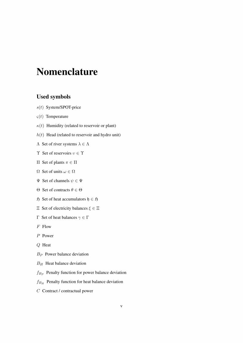
Nomenclature

Used symbols

s(t) System/SPOT-price

ς(t) Temperature

κ(t) Humidity (related to reservoir or plant)

h(t) Head (related to reservoir and hydro unit)

Λ Set of river systems λ ∈ Λ

Υ Set of reservoirs υ ∈ Υ

Π Set of plants π ∈ Π

Ω Set of units ω ∈ Ω

Ψ Set of channels ψ ∈ Ψ

Θ Set of contracts θ ∈ Θ

H Set of heat accumulators h ∈ H

Ξ Set of electricity balances ξ ∈ Ξ

Γ Set of heat balances γ ∈ Γ

F Flow

P Power

Q Heat

BP Power balance deviation

BH Heat balance deviation

fBPPenalty function for power balance deviation

fBHPenalty function for heat balance deviation

C Contract / contractual power

v

b Soft limit penalty function

K Characteristic area

x Corner point of the characteristic

m Number of convex sub areas of characteristic

n Number of corner points in convex sub area

q Heat energy within heat accumulator

qA Heat flow into heat accumulator

fq Loss heat flow function of heat accumulator

fs Area price sensitivity function

fC Cost function of procurement contract

fW Water value function of reservoir

W Water values of reseroivoir

u Status binary ∈ 0, 1

σ Spillage decision ∈ [0, 1]

η Pump decision ∈ 0, 1

δ Discharge flow of single unit

Fσ Spilled from from reservoir

Fp Pumped flow

Fr Total release from a reservoir =∑δ + Fσ − Fp

FI Local inflow to reservoir

Fc Local inflow to channel

D Channel’s time delay

Ff Total flow in channel = Fr + Fc

Fe Evaporation flow from reservoir

V Reservoir volume

h1 Reservoir water level

h2 Tail water level

fp Pump’s efficiency curve

vi

Contents

Abstract (English) ii

Abstract (Finnish) iii

Acknowledgements iv

Nomenclature v

1 Introduction 11.1 Background . . . . . . . . . . . . . . . . . . . . . . . . . . . . . . . . . . . . 11.2 Objectives and Scope of the thesis . . . . . . . . . . . . . . . . . . . . . . . . 31.3 Structure of the thesis . . . . . . . . . . . . . . . . . . . . . . . . . . . . . . . 4

2 Operational environment and business processes of balance responsible 62.1 Nordic market description . . . . . . . . . . . . . . . . . . . . . . . . . . . . 6

2.1.1 Market participants . . . . . . . . . . . . . . . . . . . . . . . . . . . . 62.1.2 Energy exchange and contracts . . . . . . . . . . . . . . . . . . . . . . 9

2.2 Description of BR’s business processes . . . . . . . . . . . . . . . . . . . . . 122.2.1 Procurement portfolio . . . . . . . . . . . . . . . . . . . . . . . . . . 122.2.2 Balance management . . . . . . . . . . . . . . . . . . . . . . . . . . . 132.2.3 Strategic planning . . . . . . . . . . . . . . . . . . . . . . . . . . . . 142.2.4 Tactical planning . . . . . . . . . . . . . . . . . . . . . . . . . . . . . 152.2.5 Operational planning . . . . . . . . . . . . . . . . . . . . . . . . . . . 15

2.3 Decision-support needs of BR . . . . . . . . . . . . . . . . . . . . . . . . . . 162.3.1 Strategic level . . . . . . . . . . . . . . . . . . . . . . . . . . . . . . . 162.3.2 Tactical and operational level . . . . . . . . . . . . . . . . . . . . . . . 16

3 Modeling of energy procurement 183.1 Notation . . . . . . . . . . . . . . . . . . . . . . . . . . . . . . . . . . . . . . 193.2 Market price and price areas . . . . . . . . . . . . . . . . . . . . . . . . . . . 193.3 Electricity and heat balance . . . . . . . . . . . . . . . . . . . . . . . . . . . . 203.4 Power and heat plants . . . . . . . . . . . . . . . . . . . . . . . . . . . . . . . 22

3.4.1 CHP plants . . . . . . . . . . . . . . . . . . . . . . . . . . . . . . . . 223.4.2 Condensing power plants and heat plants . . . . . . . . . . . . . . . . 253.4.3 Heat accumulators . . . . . . . . . . . . . . . . . . . . . . . . . . . . 263.4.4 Additional constraints in plant and unit models . . . . . . . . . . . . . 27

3.5 Unit status profiles . . . . . . . . . . . . . . . . . . . . . . . . . . . . . . . . 27

vii

3.6 Contracts . . . . . . . . . . . . . . . . . . . . . . . . . . . . . . . . . . . . . 283.6.1 Delivery contracts . . . . . . . . . . . . . . . . . . . . . . . . . . . . 293.6.2 Procurement contracts . . . . . . . . . . . . . . . . . . . . . . . . . . 29

3.7 Hydropower systems . . . . . . . . . . . . . . . . . . . . . . . . . . . . . . . 303.7.1 Reservoir model . . . . . . . . . . . . . . . . . . . . . . . . . . . . . 313.7.2 Channel and spillway models . . . . . . . . . . . . . . . . . . . . . . 343.7.3 Unit and plant models . . . . . . . . . . . . . . . . . . . . . . . . . . 373.7.4 Overall hydro system model . . . . . . . . . . . . . . . . . . . . . . . 403.7.5 Hydropower optimization sub-problem . . . . . . . . . . . . . . . . . 42

3.8 Overall model and problem formulation . . . . . . . . . . . . . . . . . . . . . 433.9 Model simplifications and assumptions . . . . . . . . . . . . . . . . . . . . . . 46

4 Information model of procurement planning problem 474.1 Theoretical overview of the information modeling . . . . . . . . . . . . . . . . 49

4.1.1 Chen’s ER model . . . . . . . . . . . . . . . . . . . . . . . . . . . . . 494.1.2 Overview of ontologies . . . . . . . . . . . . . . . . . . . . . . . . . . 514.1.3 Representation . . . . . . . . . . . . . . . . . . . . . . . . . . . . . . 524.1.4 XML and MathML . . . . . . . . . . . . . . . . . . . . . . . . . . . . 53

4.2 Information modeling applied to procurement planning problem . . . . . . . . 554.2.1 Purpose and required scope of conceptualization . . . . . . . . . . . . 554.2.2 Parametric schemas: ontology and relationships . . . . . . . . . . . . . 564.2.3 Reusability of schemas . . . . . . . . . . . . . . . . . . . . . . . . . . 56

4.3 Model component schemas . . . . . . . . . . . . . . . . . . . . . . . . . . . . 574.3.1 Abstract model components — basic entities . . . . . . . . . . . . . . 574.3.2 Constraints and soft limits . . . . . . . . . . . . . . . . . . . . . . . . 604.3.3 Markets, balances and contracts . . . . . . . . . . . . . . . . . . . . . 614.3.4 Non-hydro components . . . . . . . . . . . . . . . . . . . . . . . . . . 624.3.5 Hydro components . . . . . . . . . . . . . . . . . . . . . . . . . . . . 63

5 Discussion 65

A Overall procurement planning problem 68

B Model component schemas 70

Bibliography 75

viii

Chapter 1

Introduction

1.1 Background

Balance responsibles face a challenging problem when planning their short-term procurement.The problem is challenging for two reasons. First, the mathematical structure of the procurementplanning problem is complex despite the details of its exact formulation. Numerous technicalproblems arise with all of them, not the least being the computational burden. The second diffi-culty — the one studied in this thesis — is related to the amount and variety of the prerequisitealgorithm-independent information that plays crucial role in obtaining the solution.

Balance responsible (BR) is a player in rather turbulent electricity markets. BR carries aneconomical responsibility of physical balance between consumption and procurement within hisown balance area. This balance equilibrium sets an operational constraint, which has to be met inall situations. The operational freedom, on the other hand, is vast: BR may use any componentsavailable in his procurement portfolio — from power exchange purchases to nuclear powergeneration — to meet the balance equilibrium. However, the operational costs of different waysof procurement differ significantly. Finding the optimal strategy to utilize one’s procurementportfolio in a given situation is here referred to as BR’s procurement planning problem.

Technically procurement planning problem is very difficult. Several possible formulation ofthe overall problem or its different subsets can be found in the literature, see e.g. [1], [2], [3], [4],[5], [6], [7], [8], [9] and the references therein. Formulations as well as even the objectives varysignificantly. Generally, each formulation is custom-made for each specific solution algorithmchosen. In other words, the algorithm to be used to solve the problem is first fixed and after thata suitable model is built around that choice. Hence, as long as no specific algorithm is fixed,there is no certainty about what information is needed, that is, the information required in eachcase is formulation and algorithm specific. Besides, no general and systematic treatment of thisalgorithm-independent information has been offered.

The other source of difficulties in procurement planning problem arise from the high num-ber of different information sources that play significant roles and have profound effects on theplanning problem. That is, the high amount of essential algorithm-independent information rep-resents a considerable difficulty. Outside temperatures, spot-price forecasts, number of convexsubsets of characteristic operating areas of power units, operational limitations of units due toemissions constraints, to name just a few. All of them have to be included into inputs of an

1

optimization application as long as no specific algorithm/formulation is chosen. Maintainingan up-to-date set of all this information intelligently becomes a challenging task. Furthermore,making this information commonly available for all the necessary applications and other partiesrequires standardization of its representation. This subject has a focal part in this thesis and isaddressed in more detail shortly.

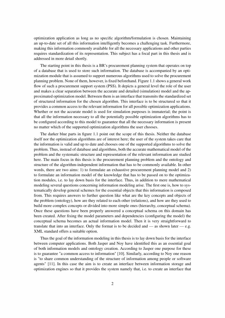
The starting point in this thesis is a BR’s procurement planning system that operates on topof a database that is used to store such information. The database is accompanied by an opti-mization module that is assumed to support numerous algorithms used to solve the procurementplanning problem. None of them, however, is fixed beforehand. Figure 1.1 shows a general workflow of such a procurement support system (PSS). It depicts a general level the role of the userand makes a clear separation between the accurate and detailed (simulation) model and the ap-proximated optimization model. Between them is an interface that transmits the standardized setof structured information for the chosen algorithm. This interface is to be structured so that itprovides a common access to the relevant information for all possible optimization applications.Whether or not the accurate model is used for simulation purposes is immaterial; the point isthat all the information necessary to all the potentially possible optimization algorithms has tobe configured according to this model to guarantee that all the necessary information is presentno matter which of the supported optimization algorithms the user chooses.

The darker blue parts in figure 1.1 point out the scope of this thesis. Neither the databaseitself nor the optimization algorithms are of interest here; the user of the system takes care thatthe information is valid and up to date and chooses one of the supported algorithms to solve theproblem. Thus, instead of database and algorithms, both the accurate mathematical model of theproblem and the systematic structure and representation of the relevant information are studiedhere. The main focus in this thesis is the procurement planning problem and the ontology andstructure of the algorithm-independent information that has to be commonly available. In otherwords, there are two aims: 1) to formulate an exhaustive procurement planning model and 2)to formulate an information model of the knowledge that has to be passed on to the optimiza-tion modules, i.e. to lay down basis for the interface. Thus, in addition to mere mathematicalmodeling several questions concerning information modeling arise. The first one is, how to sys-tematically develop general schemes for the essential objects that this information is composedfrom. This requires answers to further question like what are the key concepts and objects ofthe problem (ontology), how are they related to each other (relations), and how are they used tobuild more complex concepts or divided into more simple ones (hierarchy, conceptual schema).Once these questions have been properly answered a conceptual schema on this domain hasbeen created. After fixing the model parameters and dependencies (configuring the model) theconceptual schema becomes an actual information model. Then it is very straightforward totranslate that into an interface. Only the format is to be decided and — as shown later — e.g.XML standard offers a suitable option.

Thus the goal of the information modeling in this thesis is to lay down basis for the interfacebetween computer applications. Both Jasper and Noy have identified this as an essential goalof both information models and ontology creation. According to Jasper one purpose for theseis to guarantee "a common access to information" [10]. Similarly, according to Noy one reasonis "to share common understanding of the structure of information among people or softwareagents" [11]. In this case the aim is to create an interface between information storage andoptimization engines so that it provides the system namely that, i.e. to create an interface that

2

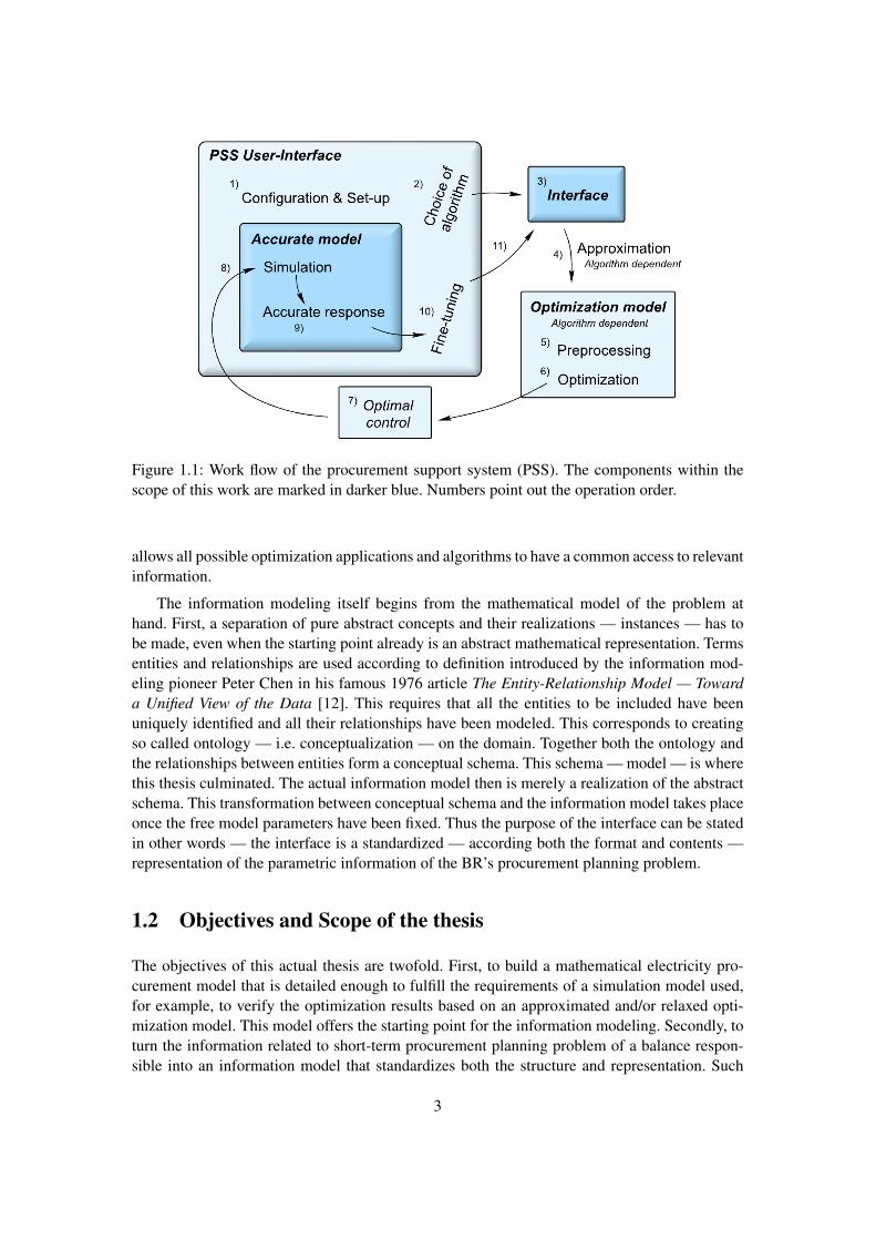
Figure 1.1: Work flow of the procurement support system (PSS). The components within thescope of this work are marked in darker blue. Numbers point out the operation order.

allows all possible optimization applications and algorithms to have a common access to relevantinformation.

The information modeling itself begins from the mathematical model of the problem athand. First, a separation of pure abstract concepts and their realizations — instances — has tobe made, even when the starting point already is an abstract mathematical representation. Termsentities and relationships are used according to definition introduced by the information mod-eling pioneer Peter Chen in his famous 1976 article The Entity-Relationship Model — Towarda Unified View of the Data [12]. This requires that all the entities to be included have beenuniquely identified and all their relationships have been modeled. This corresponds to creatingso called ontology — i.e. conceptualization — on the domain. Together both the ontology andthe relationships between entities form a conceptual schema. This schema — model — is wherethis thesis culminated. The actual information model then is merely a realization of the abstractschema. This transformation between conceptual schema and the information model takes placeonce the free model parameters have been fixed. Thus the purpose of the interface can be statedin other words — the interface is a standardized — according both the format and contents —representation of the parametric information of the BR’s procurement planning problem.

1.2 Objectives and Scope of the thesis

The objectives of this actual thesis are twofold. First, to build a mathematical electricity pro-curement model that is detailed enough to fulfill the requirements of a simulation model used,for example, to verify the optimization results based on an approximated and/or relaxed opti-mization model. This model offers the starting point for the information modeling. Secondly, toturn the information related to short-term procurement planning problem of a balance respon-sible into an information model that standardizes both the structure and representation. Such

3

an information model can then rather easily be used as an interface between a database andoptimization algorithms.

Stated more accurately in the order that they appear in this thesis, the objectives are to

1. Formulate a mathematical model of the procurement planning problem. The model is tobe detailed enough to work as a starting point for simulation model and fixes the scopefor the information modeling.

2. Identify the essential concepts — both entities and their relationships — of the problemand formulate an extensive conceptual schema to cover these. The schema is to be for-mulated bearing in mind that the information model based on it will be rendered to aninterface file using some chosen format, e.g. XML.

The problem is approached from the point of view of Nordic electricity balance responsible.This introduces some limitations on the scope of the work but generally BR may occupy multipleroles (trader, producer, etc.) and thus a rather wide perspective is gained.

Furthermore, all forecasted time series such as future spot-prices are treated as deterministicmodel parameters and no attention at all is paid on how these forecasts have been established.The model formulation is purely deterministic. This naturally implies that the model is valid onlyas a short-term planning support tool. The longer the time horizon becomes the lesser value dothese forecasts have. Of course, such hard forecast can be used as a sort of benchmarking toolsin longer time horizon planning, too. The clearest limitation in the scope of this thesis is to focusonly on the information and ignore optimization algorithms and database structures.

1.3 Structure of the thesis

The thesis is structured as follows. First, the second chapter offers the essential backgroundinformation of the BR’s operation environment and puts all things into context. The chapteroffers an overview of the electricity markets and the key players on the field. The business pro-cesses of the balance responsible are described in detail and care is taken to depict the processessignificant for procurement planning. After this the key decision the balance responsible facesduring the procurement planning are sketched, i.e. the decision support need of BR are pointedout. This acts as background information when justifying the choices made during the actualmodeling.

Chapter three takes a closer look at the components of the BR’s procurement portfolio thatplay salient roles in the procurement. Each of these is described in detail. Then a mathematicalmodel of these is formulated. The modeling is based both on literature and author’s own choices.No more than the relevant features of the model are incorporated. These the discussion proceedsto intertwine these independent model components together to formulate an overall procure-ment model. At this point this model should incorporate all the relevant information about BR’sprocurement portfolio and operation environment.

The chapter four covers the information modeling part of this thesis. It introduces the es-sential theoretical foundations and concepts. It also discusses the effects that the interface asthe goal of the information modeling sets on the scope of this task. Finally, necessary distinct

4

entities are identified and their interconnections pointed out. This results in both text format andpartly graphical representation of each model components. Together these capture both the mod-ularity and the hierarchy of the components. Rendering from this representation into interfaceimplemented in any SGML based language — e.g. XML — should be obvious.

In the last chapter the thesis is evaluated as a whole. The chapter summarizes the key aspectsand offers a critical point of view of them. It also briefly lists the made assumptions. Directionsfor further study are pointed out.

5

Chapter 2

Operational environment and businessprocesses of balance responsible

2.1 Nordic market description

2.1.1 Market participants

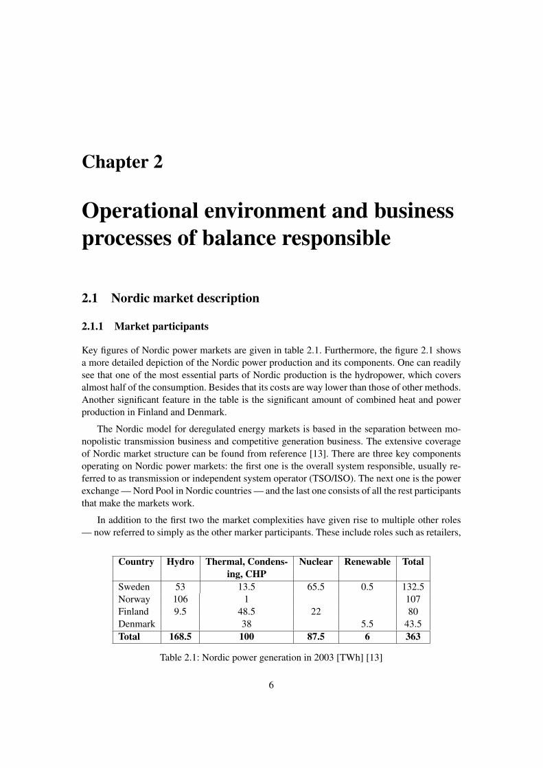
Key figures of Nordic power markets are given in table 2.1. Furthermore, the figure 2.1 showsa more detailed depiction of the Nordic power production and its components. One can readilysee that one of the most essential parts of Nordic production is the hydropower, which coversalmost half of the consumption. Besides that its costs are way lower than those of other methods.Another significant feature in the table is the significant amount of combined heat and powerproduction in Finland and Denmark.

The Nordic model for deregulated energy markets is based in the separation between mo-nopolistic transmission business and competitive generation business. The extensive coverageof Nordic market structure can be found from reference [13]. There are three key componentsoperating on Nordic power markets: the first one is the overall system responsible, usually re-ferred to as transmission or independent system operator (TSO/ISO). The next one is the powerexchange — Nord Pool in Nordic countries — and the last one consists of all the rest participantsthat make the markets work.

In addition to the first two the market complexities have given rise to multiple other roles— now referred to simply as the other marker participants. These include roles such as retailers,

Country Hydro Thermal, Condens- Nuclear Renewable Totaling, CHP

Sweden 53 13.5 65.5 0.5 132.5Norway 106 1 107Finland 9.5 48.5 22 80Denmark 38 5.5 43.5Total 168.5 100 87.5 6 363

Table 2.1: Nordic power generation in 2003 [TWh] [13]

6

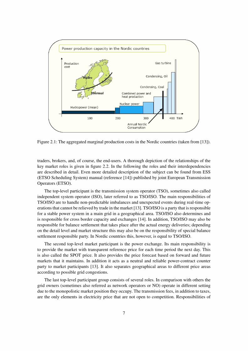
Figure 2.1: The aggregated marginal production costs in the Nordic countries (taken from [13]).

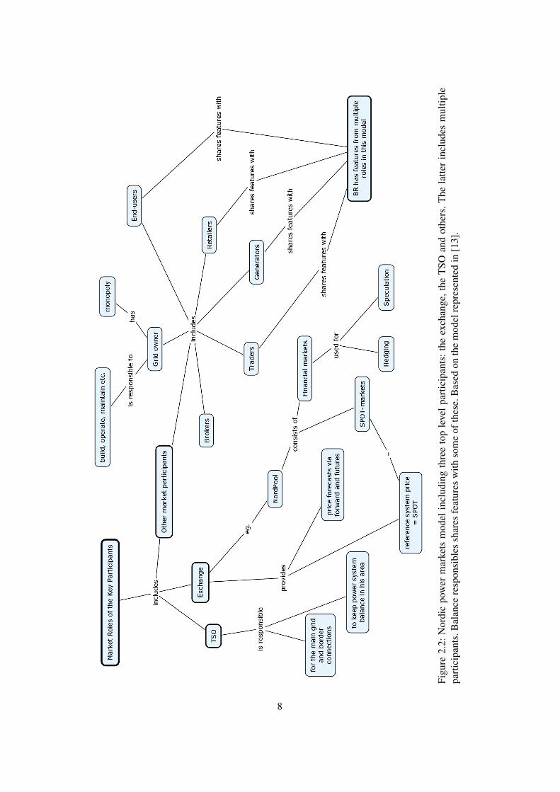
traders, brokers, and, of course, the end-users. A thorough depiction of the relationships of thekey market roles is given in figure 2.2. In the following the roles and their interdependenciesare described in detail. Even more detailed description of the subject can be found from ESS(ETSO Scheduling System) manual (reference [14]) published by joint European TransmissionOperators (ETSO).

The top-level participant is the transmission system operator (TSO), sometimes also calledindependent system operator (ISO), later referred to as TSO/ISO. The main responsibilities ofTSO/ISO are to handle non-predictable imbalances and unexpected events during real-time op-erations that cannot be relieved by trade in the market [13]. TSO/ISO is a party that is responsiblefor a stable power system in a main grid in a geographical area. TSO/ISO also determines andis responsible for cross border capacity and exchanges [14]. In addition, TSO/ISO may also beresponsible for balance settlement that takes place after the actual energy deliveries; dependingon the detail level and market structure this may also be on the responsibility of special balancesettlement responsible party. In Nordic countries this, however, is equal to TSO/ISO.

The second top-level market participant is the power exchange. Its main responsibility isto provide the market with transparent reference price for each time period the next day. Thisis also called the SPOT price. It also provides the price forecast based on forward and futuremarkets that it maintains. In addition it acts as a neutral and reliable power-contract counterparty to market participants [13]. It also separates geographical areas to different price areasaccording to possible grid congestions.

The last top-level participant group consists of several roles. In comparison with others thegrid owners (sometimes also referred as network operators or NO) operate in different settingdue to the monopolistic market position they occupy. The transmission fees, in addition to taxes,are the only elements in electricity price that are not open to competition. Responsibilities of

7

Figu

re2.

2:N

ordi

cpo

wer

mar

kets

mod

elin

clud

ing

thre

eto

ple

velp

artic

ipan

ts:t

heex

chan

ge,t

heT

SOan

dot

hers

.The

latte

rin

clud

esm

ultip

lepa

rtic

ipan

ts.B

alan

cere

spon

sibl

essh

ares

feat

ures

with

som

eof

thes

e.B

ased

onth

em

odel

repr

esen

ted

in[1

3].

8

the grid owners are merely to build, operate and maintain their networks covering geographicalareas [13]. In addition they also provide customers with connection to the grid and both gatherand submit the hourly metered values to TSO/ISO from grid’s area.

Generators usually operate both in wholesale and exchange markets. They use the latter tofine-tune their schedules as the delivery moment comes closer. Retailers (RET) may have theirown generation capacity. Hence they typically serve end-users by providing them with powereither purchased from exchange or based on their own generation. Traders do not have anyclearly defined roles since they may operate in many different market positions. In fact, all ofthe roles described here can be partly seen as traders. Traders can buy power from generator andsell it to retailers; they can buy it from other retailer and sell to another. Brokers are like tradersbut act merely as intermediates. They do not own the commodity at any moment. They, however,do not play significant role in this work. End-users on their behalf either buy their power fromretailer or if they have the necessary resources may also operate in the wholesale markets.

It is well possible that market participants have features from multiple roles sketched above.As depicted in figure 2.2 the balance responsible (BR) party may have features from generators,retailers, traders and end-users. The exact definition of the balance responsible party is that ithas an open supply contract with its TSO/ISO. This implies merely that BR has an economicresponsibility to guarantee the balance between consumption and procurement in his own bal-ance area. Balance area, on the other hand, is defined as a geographical area consisting of one ormore grid areas with common market rules and common pricing for imbalance. They are used toisolate bottlenecks between different grids [14]. This happens by introducing separate balancearea specific area prices on each of them. The prices are set on the level which is supposed toeffectively prevent the bottlenecks.

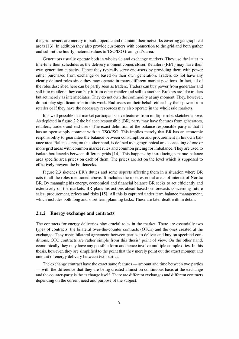
Figure 2.3 sketches BR’s duties and some aspects affecting them in a situation where BRacts in all the roles mentioned above. It includes the most essential areas of interest of NordicBR. By managing his energy, economical and financial balance BR seeks to act efficiently andextensively on the markets. BR plans his actions ahead based on forecasts concerning futuresales, procurement, prices and risks [15]. All this is captured under term balance management,which includes both long and short term planning tasks. These are later dealt with in detail.

2.1.2 Energy exchange and contracts

The contracts for energy deliveries play crucial roles in the market. There are essentially twotypes of contracts: the bilateral over-the-counter contracts (OTCs) and the ones created at theexchange. They mean bilateral agreement between parties to deliver and buy on specified con-ditions. OTC contracts are rather simple from this thesis’ point of view. On the other hand,economically they may have any possible form and hence involve multiple complexities. In thisthesis, however, they are simplified to the point that they merely point out the exact moment andamount of energy delivery between two parties.

The exchange contract have the exact same features — amount and time between two parties— with the difference that they are being created almost on continuous basis at the exchangeand the counter-party is the exchange itself. There are different exchanges and different contractsdepending on the current need and purpose of the subject.

9

Figure 2.3: Tasks of balance responsible in Nordic power markets. (Modified with additionsfrom [15].)

In Nordic countries the TSO/ISOs have established a company called Nord Pool that op-erates both the SPOT exchange Nord Pool ASA and the derivative markets. In addition, thereis also a market called ELBAS market for hour-ahead power where players from Sweden, Fin-land and Eastern Denmark can adjust their daily balances. The Nord Pool’s market environmentand general energy market flows can be seen in figure 2.4. It clearly depicts the focal position ofpower exchange in the markets and links together many of the participants described in previoussection.

Nord Pool’s spot price (ELSPOT) is based on the auction principle. Each day by 12.00 CETparticipants leave their price dependent bids for the next day. Once the bids have been receivedthe exchange computes the system price for every hour of the day to come. The system price isa so called market clearing price for it makes the offers meet the demand. Later it is referred asthe spot price.

BR’s actions on the energy exchange are not simple. Taken his role as economically re-sponsible the exchange and especially the spot price offer him a baseline to which compare hisown production costs. Figure 2.5 shows two Spot trading scenarios depending on the amountof energy from other sources. The picture clearly shows the dependence of BR’s actions on thecurrent price level. The mathematical model to be formulated has to be able to incorporate thesetypes of relationships seamlessly.

10

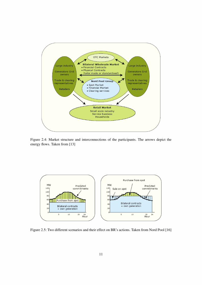
Figure 2.4: Market structure and interconnections of the participants. The arrows depict theenergy flows. Taken from [13]

Figure 2.5: Two different scenarios and their effect on BR’s actions. Taken from Nord Pool [16]

11

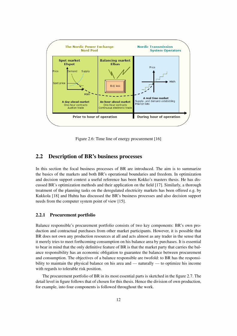
Figure 2.6: Time line of energy procurement [16]

2.2 Description of BR’s business processes

In this section the focal business processes of BR are introduced. The aim is to summarizethe basics of the markets and both BR’s operational boundaries and freedom. In optimizationand decision support context a useful reference has been Kokko’s masters thesis. He has dis-cussed BR’s optimization methods and their application on the field [17]. Similarly, a thoroughtreatment of the planning tasks on the deregulated electricity markets has been offered e.g. byKukkola [18] and Huhta has discussed the BR’s business processes and also decision supportneeds from the computer system point of view [15].

2.2.1 Procurement portfolio

Balance responsible’s procurement portfolio consists of two key components: BR’s own pro-duction and contractual purchases from other market participants. However, it is possible thatBR does not own any production resources at all and acts almost as any trader in the sense thatit merely tries to meet forthcoming consumption on his balance area by purchases. It is essentialto bear in mind that the only definitive feature of BR is that the market party that carries the bal-ance responsibility has an economic obligation to guarantee the balance between procurementand consumption. The objectives of a balance responsible are twofold: to BR has the responsi-bility to maintain the physical balance on his area and — naturally — to optimize his incomewith regards to tolerable risk position.

The procurement portfolio of BR in its most essential parts is sketched in the figure 2.7. Thedetail level in figure follows that of chosen for this thesis. Hence the division of own production,for example, into four components is followed throughout the work.

12

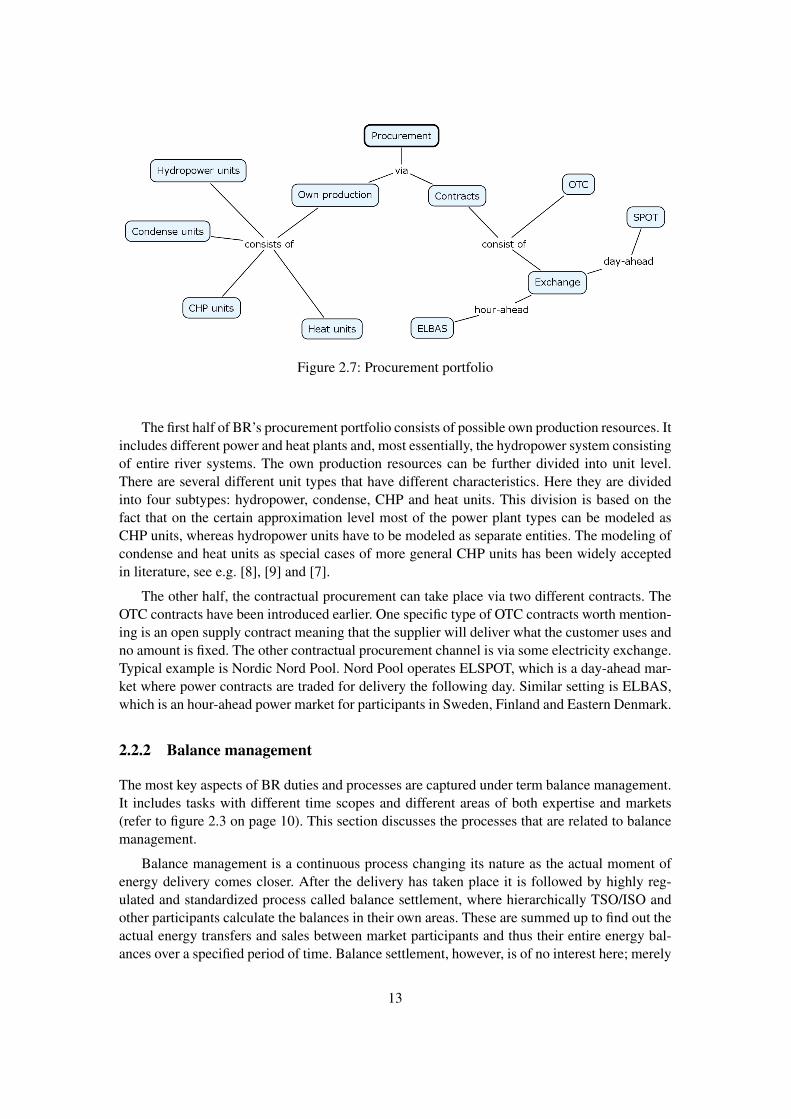
Figure 2.7: Procurement portfolio

The first half of BR’s procurement portfolio consists of possible own production resources. Itincludes different power and heat plants and, most essentially, the hydropower system consistingof entire river systems. The own production resources can be further divided into unit level.There are several different unit types that have different characteristics. Here they are dividedinto four subtypes: hydropower, condense, CHP and heat units. This division is based on thefact that on the certain approximation level most of the power plant types can be modeled asCHP units, whereas hydropower units have to be modeled as separate entities. The modeling ofcondense and heat units as special cases of more general CHP units has been widely acceptedin literature, see e.g. [8], [9] and [7].

The other half, the contractual procurement can take place via two different contracts. TheOTC contracts have been introduced earlier. One specific type of OTC contracts worth mention-ing is an open supply contract meaning that the supplier will deliver what the customer uses andno amount is fixed. The other contractual procurement channel is via some electricity exchange.Typical example is Nordic Nord Pool. Nord Pool operates ELSPOT, which is a day-ahead mar-ket where power contracts are traded for delivery the following day. Similar setting is ELBAS,which is an hour-ahead power market for participants in Sweden, Finland and Eastern Denmark.

2.2.2 Balance management

The most key aspects of BR duties and processes are captured under term balance management.It includes tasks with different time scopes and different areas of both expertise and markets(refer to figure 2.3 on page 10). This section discusses the processes that are related to balancemanagement.

Balance management is a continuous process changing its nature as the actual moment ofenergy delivery comes closer. After the delivery has taken place it is followed by highly reg-ulated and standardized process called balance settlement, where hierarchically TSO/ISO andother participants calculate the balances in their own areas. These are summed up to find out theactual energy transfers and sales between market participants and thus their entire energy bal-ances over a specified period of time. Balance settlement, however, is of no interest here; merely

13

the economical performance of BR’s procurement planning is measured in balance settlement.

Here the tasks related to balance management are divided according to the time horizonconsidered. The treatment follows that of Dyner’s [19] and the time period division is adoptedfrom him. Other sources use the same names but the exact length and duration of the periodsis not always the same. The time periods have different characteristics and require differentcustomized planning methodologies. Beginning from the most difficult and far-reaching theperiods are strategic, tactical and operational. The strategic planning includes the most long-range decisions like business alliances, capacity investments and long-term contracts. Tacticaldecisions include aspects like short-term contracts, brand management and fuel contracts. Thelast level is operational, which includes short-term — almost real-time — decision like biddingprices and strategies and real-time balance monitoring.

In the following each of these main time horizons is dealt individually. With each of thetime horizons also the general methodologies applicable to such planning tasks are briefly stated.Used planning methods critically depend on the time horizon: on the long-term the only suitablemethods are hard modeling , strategic simulation and scenario analysis. At the short-term levelhard modeling might be accompanied by different gaming analysis. The following discussion ismostly based on the overview offered by Dyner [19].

2.2.3 Strategic planning

Strategic planning is a wide-ranging process including aspects from the entire organization. Itmight include time horizons from one year even to over a decade. Hence concentrating merelyon balance management related strategic decision is difficult if not impossible. The huge uncer-tainties that the BR faces in long-term planning rise from several sources: the uncertainties inweather, production, consumption, and prices.

Typical strategic decisions organizations face are related to acquisitions, alliances and otheroperations that have a strong effect on company’s market position affecting long periods of time.In case of balance responsible and especially its balance management the most evident strategicdecisions are related to capacity investments and possible long-term contracts [15].

Due to the long time period it concerns and enormous uncertainties the applicable strategicplanning methodologies are limited. According to Dyner [19] the most suitable methodologicalapproaches consist of strategic simulation, scenario analysis and to some extent of hard model-ing techniques, i.e. traditional optimization methods. The scope of the latter, however, is limitedand serves best as a sort of benchmarking method. Hence, Dyner’s comments do not encour-age the procurement optimization point of view adopted in this study to be used for strategicplanning.

The inputs into strategic level planning depend both on the time horizon included and onthe focus and the subject under study. Within shorter-term inspections decision maker mightbe interested in things like future price developments, currency rates and interest levels. On alonger level, though, these aspects might turn out to be merely unnecessary details. In the lattercase the only inputs might be total production capacity and overall market parameters such aslong-term price changes and possible government policy changes.

The decision maker looking this far into future seeks to find insight into effects of drasticchanges in market parameters that he both is and is not able to have an effect on. Hence scenario

14

analysis plays a crucial role in investigations like this. Scenario analyses combined with hardmodeling used for benchmarking purposes are what the solutions offered in this study are bestaimed for.

2.2.4 Tactical planning

BR’s tactical level — medium level — planning deals with issues such as short-term contracts,fuel contracts, brand management, risk management, insurance costs, hedging, budgeting andplant revision schedules [15]. It includes time horizons from a few weeks to year level. Primarilyit aims at accumulation of deep understanding of the markets and its dynamics. According toDyner neither this can be done exclusively with hard simulation methods.

Planning on yearly level and especially with longer time horizon deals more or less withspeculative issues and what-if situations. Since the time scope efficiently prohibits any exactinformation the planning on this level still has substantial uncertainties and hence tends to berather qualitative on its nature. The main focus is rather to be on risk management. Thus thedifferences compared with strategic planning are rather conceptual yet clear.

The key aspects on this level are forecasts for price developments, the procurement basedon it and reserved resources [15]. Essential issues directly related to production and hence alsoto procurement are the plant revisions. As the market price level forecasts gain accuracy BR isable to forecast his forthcoming obligations and begin to plan his production and contractualprocurement to reduce the gap between those.

Risk management relates to this level planning seamlessly, yet it is left out of scope of thisstudy. The market instruments used with this purpose in mind include financial contracts likefutures and options.

Inputs into tactical level planning include future price forecasts, already fixed plant revi-sion schedules, reserved production resources and overall view of market situation includinghydrological aspects [15]. All these are more or less inherently stochastic variables and mod-els. Output is used as guidance in more subtle investigations as the moment of energy deliverycomes closer.

2.2.5 Operational planning

The operational level planning — or short-term planning — is the most proper ground for hardmodeling techniques like the procurement optimization methods developed here [19]. The timehorizon of interest here ranges from almost real-time operations to a few weeks and deals with amultitude of aspects. The main interest is more clearly on the optimal use of BR’s procurementportfolio as in the two previous levels have concentrated more on optimal form of this portfolio.

The key concepts and inputs on this level are BR’s own production forecast, spot salesforecast, the current OTC contracts [15] and other consumption related issues such as weatherforecasts and fuel reserve status [6]. At the later point in time these forecast will turn into realizedtime series, yet the nature of the optimization in this work hardly changes since all stochasticcharacteristics are ignored in the first place. Based on the mentioned inputs the daily bids aresubmitted to the exchange and other market participants informed according to regulation rules.

15

Once the exchange trading has realized BR’s planning faces drastic changes as the plansthat this far were based on forecasted market price now change into real physical and econom-ical obligations. From procurement point of view the change, however, is profound. The dailyrealization of spot trading into concrete obligations also brings a new input into the model: therealized obligations now have to be dealt with different attitude than they were before.

Once the spot based contracts are known the trading may still continue depending on themarket setting. The possible regulation energy deliveries take place when ordered by TSO/ISOwith hour-ahead markets like those on ELBAS. Furthermore, depending on the market settingit might also be possible — like in Finland, for example — to adjust one’s own generationportfolio real-time in seek for optimal balance results.

The last time level to deal with is the real time operations. The real-time balance manage-ment includes possible ELBAS trading, responses to regulation energy demands from TSO/ISOand overall balance bias monitoring. These aspects, however, do not play significant roles in thisthesis because the time horizon simply becomes too short for any decision support consideredhere.

2.3 Decision-support needs of BR

Depending on the planning time horizon the BR faces different and recurrent key decisions. Herewe summarize those and point out the ones that the procurement planning solution presentedhere is applicable.

2.3.1 Strategic level

Two most fundamental issues arising in strategic planning context are capacity investments andall sorts of long-term contracts. The first includes all capital-intensive investment decisions thathave an effect on company’s long-term competitive status.

The other category of long-term planning composes different scenarios that are used to try,speculate, and iterate different market scenarios. Adjusting market parameters and investigatingcompany’s performance in multitude of cases helps decision makers to gain insight into thedynamic relations on the market. Scenario analysis combined with hard modeling techniquesand possible different decision trajectories provides at least a valuable tool for benchmarkingleast acceptable performance measures [19].

In brief the key decision on strategic planning level are 1) whether or not to invest and whento invest on new capacity, 2) what are the long-term consequences of certain contracts, 3) whatare the consequences of changes in certain market parameters, and 4) what are the joint effectsof possibly all these issues.

2.3.2 Tactical and operational level

Key decisions on tactical planning level concentrate on more concrete decision problems thanthe more speculative and qualitative strategic ones. Planning of the plant revision schedules inadvance is essential part of this level operations. Due to possibly high shut-down and start-up

16

costs the revision schedules have significant impact on the financial figures of the BR. Anotherissue are the contracts. Both medium-term OTC and fuel contracts have to be included in theanalysis. OTC contracts play an essential role here. They set the essential boundary conditionsto all succeeding decisions. Long-term fuel price changes are, of course, of strategic interest;here, however, decision maker is more interest on short-term effects of price fluctuations and hiscontractual position.

In addition, also hedging and general risk management are of interest on this level of plan-ning. Significant uncertainties and risks are introduced by several independent factor such ascurrency and Spot-price variations, credit and operational risks, to name of few. Most of this,however, is included under the term risk management. It is inseparably intertwined with strate-gic planning and utilizes a vast set of different methods. In this thesis it is not considered anyfurther.

As the time horizon becomes shorter the BR’s hands become more and more tightly tied. Atthe same time the amount of essential details increases but the forecast gain more accuracy. Twoessential categories of decisions in short-term planning are the bidding on the Spot-markets andthe exact running directives of the components in BR’s procurement portfolio. The first one isan art on itself and no further attention is paid for it.

Establishing accurate running directives for the production resources in changing environ-ment is the problem studied closely in this thesis. To put it briefly: the main issue on operationallevel is how to use BR’s procurement portfolio in an optimal manner given the forecasted marketconditions.

17

Chapter 3

Modeling of energy procurement

The detailed model of the procurement planning problem is developed here. The purpose ofthe model is twofold: first, it sets basis for an extensive simulation model used, for example, toverify the results given by approximated optimization models. Secondly, it reveals the essentialalgorithm-independent information needs of the general optimization application, that is, theontology of the planning problem is formulated based on information that comes up here. Inother words, the model is used to introduce the essential focal bits of information in meaningfulcontext.

The model will be complex. There are several different components and all of them havedifferent characteristics. Many different constraints and equations will be found. To keep trackof them all poses an additional problem on used notation. Thus excessive care is taken to ensurethat the notation will be both compact yet versatile.

The chapter is structured as follows. The discussion is divided into sections and each ofthem covers a single component of the procurement portfolio. First, however, market-relatedsubjects are treated. Both electricity and heat balances are introduced. Then the typical thermalproduction plants are presented. They are followed by both delivery and procurement contracts.The most important and complex part of the chapter is the hydropower model. It is discussedthoroughly because it forms an important yet independent component in the procurement port-folio.

In the last section all the components are intertwined and a general BR’s procurement plan-ning problem in formulated. The formulation, however, is not a waterproof optimization prob-lem even though it quite closely resembles one. It is merely meant to be a way to introduce theessential characteristics of the problem, i.e. to point out which variables are model parametersand which decision variables.

The formulated model is continuous in time. This choice cannot be justified from the op-timization point of view; the time-continuous model would be dramatically too complex andcomputationally expensive to be optimized in practice. However, in this case the choice is basedon the compactness and intuitively appealing representation. The transformation from contin-uous model into discrete is rather trivial. Besides, the continuous model is straightforward tosimulate even if some of its functions were discontinuous.

18

3.1 Notation

Since the main emphasis in this thesis is to develop an information model an extensive care istaken to formulate the presentation bearing this aim in mind. In practise, this means that thenotation is close to both relational and object-oriented way to represent information. Hence thenotational power within the mathematical set theory is used; a division between classes andtheir instances is made right from the beginning. This also corresponds to the treatment laterin the information modeling part, where distinction between abstract entity classes and theirrealizations — instances — is made.

For example, in hydropower context class symbol Υ (Greek capital upsilon) is used to rep-resent collection of all reservoirs. Specifying a single river system λ all reservoirs belonging tothis particular river system can be denoted by Υλ where the lower index is used to point out thatthe class in question is a subset of the original class. A single reservoir is denoted as an instanceof this class: υ ∈ Υ. To point out a specific reservoir a lower index i is used: υi ∈ Υ. Now,with each reservoir there is an associated power plant. The collection of all power plants withinmodel is notated with Π. Each power plant, on its behalf, consists of arbitrary number of units— collection of whose is notated as Ω. With agreed notation it is easy to express things like allunits of the plant π: ω ∈ Ωπ.

For the sake of conformity and readability the notation has been extended to include func-tional relationships and other parameters that come up in the model. Functions are generallyreferred to with letter f . It has two subscripts, e.g:

fh1,υi(t)

the first one specifies the function, e.g h1 meaning that the function is related to a reservoir’swater level h1. The second one specifies to which particular object the function refers to, e.g υimeaning that the reservoir in question is υi.

Similarly, flow notationFf,ψj

(t)

stands for the flow within channel ψj (capital F for flow, f for particularly flow within channel).As a general rule capital P denotes power, C contractual power (equivalently contract) and bpenalty function from soft limit violation. Similarly, K stands for a characteristic area of a unit.

Refer to the Abbreviations and acronyms-page in the beginning of this thesis for completelist of used notation.

3.2 Market price and price areas

The starting point for procurement optimization is the market price s(t). However, there areseveral different price areas that all have their own market prices, referred to as area prices.Differences in area prices are due to transmission limitations and thus introducing price areasone does not have to worry about limitations in transmission capacity. Finland, for example,consists of a single price area.

19

Set of all price areas is referred to as Ξ. Each price area ξi ∈ Ξ has its own area price sξi(t).Since there is a one-to-one correspondence between price areas and area prices the price areagroup Ξ is equivalent to a group of area prices.

The market price of each price area is taken as a parameter in the model. It is assumed tobe a fully deterministic time series and no further attention is paid on how this forecast hasbeen established. The markets are modeled simply via the market price sensitivity to the totalproduction of the BR. In case of a BR that is small in terms of his own production capacitythe most suitable approximation is naturally market price that has no dependency on the BR’sproduction. On the other hand, in the case of a significant producer the market price may varysubstantially due to the changes in BR’s forecasted production. Mathematically, in the mostgeneral form possible, this dependency is given as a function that maps the situation on whichthe price estimate was based and the deviation from it onto the new market price. The newsystem price in the price area ξ is then

sξ(t) = fs,ξ(sold,ξ(t), Pold,ξ(t), Pnew,ξ(t)) (3.1)

where sold,ξ(t) denotes the old price forecast on price area ξ given the old production planPold,ξ(t).Once net amount of own production changes to Pnew,ξ(t) this function gives the new price levelestimate.

3.3 Electricity and heat balance

There are two types of balances in this work. In addition to power balances also the heat balancesplay crucial roles from a point of view of a Nordic BR. Significant amount of combined heatand power production in Nordic countries (see table 2.1) is an additional limitation to operationof CHP plants and also other plants within the same power and heat balances: BR has to alwaysconsider also the heat generation and the features it incorporates into the model.

A power balance is an equation that binds the production and consumption together, i.e.procurement equals to consumption. This is due to the physical fact that it is not possible to storeelectrical energy in significant amounts. Heat, ont the other hand, is more complex commoditysince it can be stored to be used later. The heat storage is called a heat accumulator and isdiscussed later in subsection 3.4.2.

The optimization problem BR faces is how to harvest one’s procurement portfolio in orderto meet the forecasted consumption that is due to contractual obligations. BR either producesthe power himself or buys it; compare to figure 2.7 on page 13.

Denoting BR’s total own production into the grid at time t by P (t) and similarly the netexchange trade by S(t) one can represent the power balance equation as

P (t) + S(t) = C(t)

where C(t) stands for consumption —or more accurately: physical contractual position— attime t. In practice, this means that the trade S(t) is a decision variable that denotes the amountof power that is either sold to or bought from others at market price via power exchange. S < 0obviously means that the BR produces more than obligated and the excess is sold. Consideringthe BR’s work flow introduced in the previous chapter it also is evident that no exchange trade

20

at the market price is possible after the spot-trading has ended for the day, i.e. S(t) = 0 t <tspot end time. This neglects the possibility of the ELBAS type of trading but modeling this isconsidered to be out of the scope here. C(t), on the other hand, represents sum of both allrealized contracts that have become obligations and the set of available procurement contracts.The latter may involve decision variables, i.e. decisions how much to harvest one particularprocurement contract. This is more thoroughly discussed in section 3.6 As daily SPOT-tradingrealizes into contractual obligations they are not any longer present in the trading term S butinstead appear in contractual position C. This becomes more evident in section 3.8 when thegeneral procurement optimization problem is formulated.

The contractual obligations C(t) consist of both bilateral and spot contracts — and bothdelivery and procurement contracts. Even though the delivery obligations are not completelyknown all of them — and hence also the entire term C(t) — are assumed to be fully determin-istic time series. Thus it does not make any difference whether they are thought of as forecastsor deterministic time series; the consumption related to them is simply taken for granted.

In fact, the above balance equation naturally holds for each of the separate balances, that is,for each balance area ξ:

Pξ(t) + Sξ(t) = Cξ(t) ∀ ξ ∈ Ξ (3.2)

The notation should be trivial.

Unlike with power balance BR’s hands are more tightly tied with heat balance. A single heatbalance is denoted by γ whereas the set of all heat balances is Γ. There is no general marketplace where to buy or sell heat; heat can be transferred only within the local district heatingnetwork. Thus the production and net heat flow of the accumulators have to be equal to the heatload forecast of the balance γ which is denoted by CH,γ(t) — it is taken as a fully deterministictime series similarly as the contractual power position C(t) is. Heat accumulators h ∈ H bringa little more flexibility.

Denoting the total heat production into the balance γ by Qγ(t) and the net flow into theaccumulators within this balance by qA,γ(t) the balance equation for each balance can be writtenas

Qγ(t) + qA,γ(t) = CH,γ(t) ∀ γ ∈ Γ (3.3)

The above power and heat balance equations turn out in practise to be quite idealistic. Firstof all, such ideal situation hardly can be found in real life; unexpected balance biases are likelyto emerge. Secondly, considering the mathematical model only, an additional problem arises:sudden discontinuities in contractual position, for example, may force the other variables tounrealistically dramatic sudden changes when the system is trying to compensate them. Thereare limits on the change rate of the output levels of the units, naturally. Thus the only way tointroduce corresponding discontinuities in the production side as well may result in unnecessaryunit start-ups or shut-downs. The third issue worth considering within this context is that quitenaturally BRs may encounter situations where meeting the heat balance, for example, simply isnot possible or rational.

With the three points in mind it is now justified to introduce an additional deviation term inthe balance equations to relax them to be more functional in such cases. Hence, the equations

21

get the form

Pξ(t) + Sξ(t) = Cξ(t) +BP,ξ(t) ∀ ξ ∈ Ξ (3.4)

Qγ(t) + qA,γ(t) = CH,γ(t) +BH,γ(t) ∀ γ ∈ Γ (3.5)

where BP,ξ(t) and BH,γ(t) represent the deviation in the power and heat balances, correspond-ingly.

The balance deviations have to be penalized but the realistic penalties are not trivial. Inelectricity case the cost of the balance power delivered by TSO/ISO (found out in balance set-tlement) offers natural and easily justified option because the price of the balance power is setso that it is not economically reasonable to use it [20]. Hence, given current balance power priceestimate fBP ,ξ(sξ(t)) the balance deviation can be penalized in the objective functional.

In case of the heat balance the cost of balance deviations is not that straightforward. Hence,rather generally, in this case it is just assumed that a corresponding penalty function fBH ,γ(t)can be formed.

3.4 Power and heat plants

In comparison with the hydropower system represented later the other power components of theprocurement portfolio constitute a rather more static entity. Unlike in hydropower case here thepower plants are relatively independent, Their only intertwining concepts are the power and heatbalances and the market prices.

There are three types of non-hydro power plants and units in this model: pure power sources(condensing plants), pure heat sources, and their combination, i.e. CHP plants. Since the firsttwo can be treated as a special case of the last one (this becomes obvious later) the descriptionnaturally begins with the CHP plants.

Each unit type has different characteristics both in production and its costs. Production isdiscussed with each plant type in the following. The discussion ends with introduction of the socalled characteristic area of the power units that is a widely accepted model of the power units.

3.4.1 CHP plants

Combined heat and power (CHP) production facilities represent the most general and exten-sive power plants within this model. They play focal roles in the optimization problems thatincorporate both the heat and power balances. Since the heat and power outputs of the plant areintertwined their running programs are more complex than those with only one output.

A plant πj is merely a collection of units ωi ∈ Ωπj . Still it has its own part in the model sincethere exists constraints for the whole plant in addition to those of units. In practise, however,there typically exists only one unit per plant in non-hydro cases. In hydropower context thesituation is different and thus the seemingly useless plant-unit-division is utilized here, too.

Each CHP unit is capable of producing both heat Q and power P . Hence, the pair (P,Q)could be directly taken as decision variable; or more clearly both the power and heat outputcould be decision variables.

22

The set of the possible combinations of power P and heat Q is called the feasible operationregion of the unit. Formally, its is a subset of the (P,Q)-plane and is called the characteristicarea — or briefly, the characteristic Kω — of the unit ω:

Kω (P,Q) (3.6)

For now the characteristic is allowed to be of any form but in the following subsection a differentformulation is introduced.

CHP units modeled via partially convex characteristics

Modeling the CHP plants via characteristic is a widely accepted way to represent the cost infor-mation and operational limitations of a CHP plant [1] [2], [17]. Here, however, it is also requiredto compose of finite number of convex sub areas. In other words, the characteristic K is not re-quired to be convex itself but it is assumed that it is possible to decompose it into finite numberof convex sub areas. This approach is originally discussed by Makkonen and Lahdelma in [2].

Each unit ω has its own status binary uω(t). This binary is a decision variable that determineswhether the corresponding unit is up and running, i.e.

uω(t) ∈ 0, 1 ∀ t (3.7)

There are several aspects and difficulties in actually determining the optimal status profiles ofthe units. These are discussed in more detail later.

Now, suppose that the characteristic Kω is decomposed into mω convex subareas. These arenumbered from 1 tomω and each of them has a corresponding area binary variable vω,i(t) : i ∈1, . . . ,mω, where each vω,i(t) ∈ 0, 1 ∀t. This binary is used to point out on which of thesubareas the plant currently operates.

Now, requiring that the sum of all area binaries equals to the status binary, i.e.

mω∑j=1

vω,j(t) = uω(t) (3.8)

guarantees two things: first that the unit operates only on one subarea at a time, and secondlythat while the unit is down it does not operate on any of them.

Furthermore, suppose the sub area i composes of nω,i corner points xω,i,j(t) : j ∈1, . . . , nω,i. These corner points are defines as elements in R2:

xω,i,j(t) = [Pω,i,j(t), Qω,i,j(t)]> (3.9)

Thus the subarea is defined by this set of its corner points. The operating point within the singlesub area can hence be given as the convex combination of these points as

x(t) =nω,i∑j=1

wω,i,j(t) xω,i,j(t), (3.10)

wherewω,i,j’s are the convex coefficients of the combination andwω,i,j ≥ 0 ∀i, j and∑ni

j=1wω,i,j =1 ∀i. The resulting operation point can thus be decomposed into xω(t) = [Pω(t), Qω(t)]>.

23

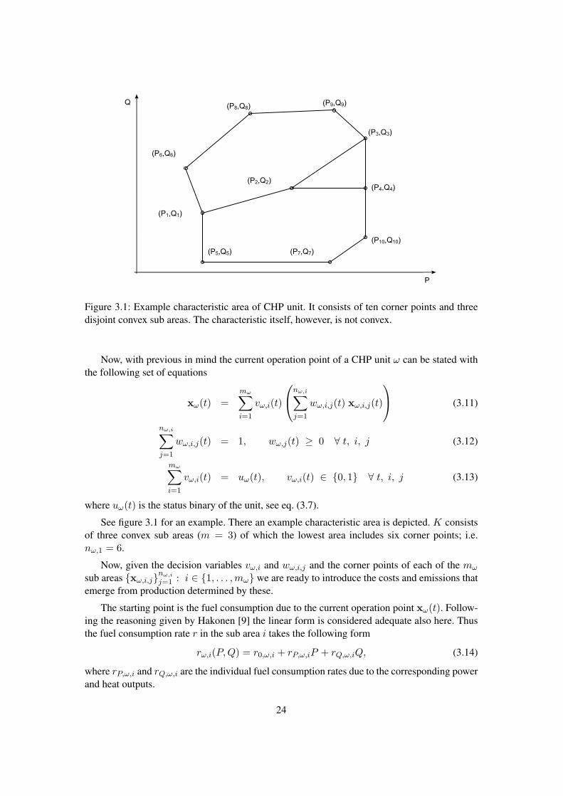
Figure 3.1: Example characteristic area of CHP unit. It consists of ten corner points and threedisjoint convex sub areas. The characteristic itself, however, is not convex.

Now, with previous in mind the current operation point of a CHP unit ω can be stated withthe following set of equations

xω(t) =mω∑i=1

vω,i(t)

nω,i∑j=1

wω,i,j(t) xω,i,j(t)

(3.11)

nω,i∑j=1

wω,i,j(t) = 1, wω,j(t) ≥ 0 ∀ t, i, j (3.12)

mω∑i=1

vω,i(t) = uω(t), vω,i(t) ∈ 0, 1 ∀ t, i, j (3.13)

where uω(t) is the status binary of the unit, see eq. (3.7).

See figure 3.1 for an example. There an example characteristic area is depicted. K consistsof three convex sub areas (m = 3) of which the lowest area includes six corner points; i.e.nω,1 = 6.

Now, given the decision variables vω,i and wω,i,j and the corner points of each of the mω

sub areas xω,i,jnω,i

j=1 : i ∈ 1, . . . ,mω we are ready to introduce the costs and emissions thatemerge from production determined by these.

The starting point is the fuel consumption due to the current operation point xω(t). Follow-ing the reasoning given by Hakonen [9] the linear form is considered adequate also here. Thusthe fuel consumption rate r in the sub area i takes the following form

rω,i(P,Q) = r0,ω,i + rP,ω,iP + rQ,ω,iQ, (3.14)

where rP,ω,i and rQ,ω,i are the individual fuel consumption rates due to the corresponding powerand heat outputs.

24

The cost resulting from this is then given as

cω,i(r) = c0,ω,i + cr,ω,i r (3.15)

After defining rω,i = [rP,ω,i, rQ,ω,i]> and substituting equation (3.14) into (3.15) we obtain thefollowing form for the current operation cost of the unit ω operating in sub area i

cω,i(t) = c0,ω,i + cr,ω,i(r0,ω,i + r>ω,i xω(t)) (3.16)

Furthermore, using the area binaries vω,i(t) the overall operation cost of the unit ω can be givenas

cω(t) =mω∑i=1

vω,i cω,i(t). (3.17)

This formulation — rather implicitly — guarantees that the operation cost of unit is zero whileit is off-line, i.e eq. (3.13) requires

∑mωi=1 vω,i(t) = uω(t) = 0.

It is easy to extend the previous discussion to cover also the emissions resulting from theproduction. It is quite natural to assume that the emissions emerge only from fuel usage, i.e theyare directly proportional to the fuel consumption. Hence, analogically to eq. (3.15) the currentemission are expressed as

eω,i(r) = e0,ω,i + er,ω,i r (3.18)

and similarly — following eq. (3.17) — the total emissions

eω(t) =mω∑i=1

vω,i eω,i(t). (3.19)

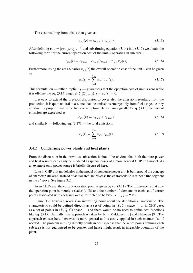
3.4.2 Condensing power plants and heat plants

From the discussion in the previous subsection it should be obvious that both the pure powerand heat sources can easily be modeled as special cases of a more general CHP unit model. Asan example only power source is briefly discussed here.

Like in CHP unit model, also in the model of condense power unit is built around the conceptof characteristic area. Instead of actual area, in this case the characteristic is rather a line segmentin the P space. See figure 3.2.

As in CHP case, the current operation point is given by eq. (3.11). The difference is that nowthe operation point is merely a scalar (∈ R) and the number of elements in each set of cornerpoints associated with each sub area is restricted to be two, i.e. nω,i = 2 ∀ i.

Figure 3.2, however, reveals an interesting point about the definition characteristic. Thecharacteristic could be defined directly as a set of points in (P,C)-space — or in CHP case,as a set of points in (P,Q,C)-space — and there would be no need to define cost functionslike eq. (3.17). Actually, this approach is taken by both Makkonen [2] and Hakonen [9]. Theapproach chosen here, however, is more general and is easily applied in such manner also ifneeded. The problem in using directly points in cost space is that the set of points defining eachsub area is not guaranteed to be convex and hence might result in infeasible operation of theplant.

25

Figure 3.2: Example characteristic area of a pure power unit with mapping from this area on tocost space c. The characteristic area is in this case only the range of the feasible region on the P -axis. It consists of four corner points and three disjoint convex sub areas (m = 3). Compare withfig. 3.1. Here, also the area and corner point indexes are visible.

3.4.3 Heat accumulators

The heat accumulators are a way to store heat energy to be used at a more appropriate time.They hence introduce a mechanism to make more rapid changes possible in power production.Single heat accumulators are denoted by h whereas the set of accumulators is H.

Formally, a heat accumulator h has a state describing the energy it contains, here denotedby qh(t). It is associated with the decision variable qA,h(t) that tells the heat flow into the ac-cumulator — and the with negative sign the flow out from the accumulator. In addition to thisthere are some heat losses that depend on the outside temperature.

With these the system equation of a heat accumulator with the initial value gets the form

qh(t) = qA,h(t)− fq,h(qh(t), ς(t)), qh(0) = q0,h (3.20)

The amount of energy that can be stored in accumulator is naturally bounded. Equally, alsothe input and out-take rates are bounded:

qh(t) ∈ [ qminh (t) , qmax

h (t) ] (3.21)

qA,h(t) ∈ [ qminA,h(t) , q

maxA,h (t) ] (3.22)

The same applies to the control variable as well. They, however, may also depend on thecurrent value of the state variable qh(t):

qA,h(t) ∈ [ dqminA,h(qh(t), t) , dq

maxA,h (qh(t), t) ] (3.23)

In practice, this constraint guarantees that the optimization does not result in bang-bang controls.

In the following the also the notation qA,γ(t) for net flow into all accumulators within heatbalance γ is used.

26

3.4.4 Additional constraints in plant and unit models

In addition to the constraints laid down to limit each unit’s feasible operation region in (P,Q)-plane (eqs. (3.12) and (3.13) on page 24) there are a few other significant constraints to beincluded into the model.

The essential dynamic constraints set limits on the change rates of the units. Formally, theseare naturally derivative constraints on the power and heat outputs of the units:

∂Pω(t)∂t

∈ [ dPminω (t) , dPmax

ω (t) ] (3.24)

∂Qω(t)∂t

∈ [ dQminω (t) , dQmax

ω (t) ] (3.25)

In the case of pure power or heat sources the partial derivatives simply reduce to time derivatives.

The derivative constraints are time dependent to guarantee the most general setting for theinformation model. Possible hardware upgrades, for example, may result in changes in theselimits during planning period. Hence the time dependency is grounded. If not necessary theycan simply be replaced with constants.

In some countries there are tax consequences if the plant’s yearly power output exceedssome specific amount. Thus, in such cases it is important for the decision maker to be able totake these aspects into account in the long-term planning.

Formally, such a restriction for plant π can be stated as∫ t2

t1

∑ω∈Ωπ

Pω(t) dt ≤ Pmax,π, (3.26)

where Pω(t) is the first element of the vector xω(t) in eq. (3.11) and Pmax,ω is a parameter ofthe model.

Alternatively, the restriction can be treated as a soft constraint with an additional penaltyterm incorporated into the objective functional. This case, however, is not included here.

Another significant restriction on the plant π is the need to restrict its cumulative yearlyemissions. Formally the constraint is of the form∫ t2

t1

∑ω∈Ωπ

eω(t) dt ≤ emax,π, (3.27)

where eω(t) comes from the eq. (3.19) and emax,ω is a parameter of the model.

3.5 Unit status profiles

Scheduling the plant and unit revision is generally referred to as the unit commitment problem.It is a typical dynamic programming problem [21]. The difficulty lies in the fact the the problemis inherently dynamical and the traditional dynamic programming formulations suffer from thecurse of dimensionality [22].

27

Here each unit has its own unit status profile (binary) uω(t) ∈ 0, 1 ∀t. See eq. (3.7) onpage 23 and the following material for its role in the unit modeling. Here the properties of thestatus profile are examined further.

Each moment of time that the unit ω changes its status is denoted either as the shut-downtime td,ω or start-up time tu,ω [9]. The time interval between them is — correspondingly —called either down- or up-time. These are unit-dependent constants that impose constraints onthe units status behavior. The minimum down-time after shut-down and before the next start-upis denoted by tmin

d,ω . Correspondingly, the minimum up-time is tminu,ω. Physically they arise from

the mechanical properties of the units that require certain time of steady operation before thenext status change is possible [8].

Depending on the length of the time interval tu − td between the shut-down and start-upthere are costs associated with the start-up. They cover two things. First, the direct costs dueto the increased fuel consumption during start-up and secondly, also the indirect costs that aregenerated because the start-up results as an additional load on the machinery that hence requiresmore maintenance. The colder the unit gets — i.e. the longer it stays down — the more the nextstart-up is going to cost [8].

The start-up costs hence are essential to realistically take into account the physical lim-itations of the units and also the prevent the optimization solution from converging towardsunrealistic bang-bang controls, i.e. rapid and continuous status changes.

Here the start-up cost of unit ω as a function the the down-time are denoted by cs,ω(td,ω, tu,ω).Kakko [8] has introduced an exponential formulation of the cost function as

cs,ω(td,ω, tu,ω) = cs1,ω(1− e−cs2,ω(td,ω ,tu,ω)) + cs3,ω, (3.28)

where cs1,ω stands for the cold-start-up cost of the boiler, cs2,ω is the time constant of the boiler’stemperature loss and the cs3,ω is the start-up cost of the turbine. This formulation is adopted here,also.

A similar situation arises later with the pumping binary η(t) in hydro power context, also.The pumps, however, play minor role here and hence they are not treated with similar detail.The discussion, however, could be applied to them, too.

As the unit status binaries actually are state variables of the model there naturally has to beat least the initial values for them. Hence, for each unit also the value u0,ω ∈ 0, 1 is defined.Possibly, there also may be the end condition u1,ω ∈ 0, 1. In case the entire plant π is to bescheduled off-line for some reason then simply uω = 0 ∀ ω ∈ Ωπ.

The actual optimization model incorporating these aspects, however, is not formulated here.Since the model presented here is used merely to point out the information needs of the infor-mation model and to simulation purposes there is no need for that. The latter can be achievedeven without explicit modeling of these aspects. Simply the knowledge about the status profileis all that is needed.

3.6 Contracts

In addition to own production the other side of the BR’s procurement portfolio consists of con-tracts. Despite that only BR’s energy procurement has been discussed so far, here also the con-

28

tractual delivery obligations are considered. There are two types of contracts that are of interestin this case First, there are the delivery contracts, that is, BR has a contractual obligation todeliver energy. The time profile of the delivered power may depend on the usage of the counter-party and thus at the best BR has only a forecast of the amount to be delivered. In this case,however, these forecasts are treated as deterministic time series. The other set of contracts arethe procurement contracts, that is, BR has right to take energy from the counter-party. The con-tracts may fix the time and the power profile or —- more general case — they may be modeledas BR’s decision variables. Formally, this means that the contractual C(t) position is dividedinto two parts:

C(t) = Cd(t)− Cp(t)

where Cd(t) refers to delivery obligations and Cp(t) to procurement contracts. As shown abovethe net contractual position is their sum. A thorough treatment of contracts on energy sector isgiven by Lahtinen [23].

Notationally, the set of all contracts is denoted by Φ, where naturally one contract is φ ∈ Φ.Likewise, the set of contracts on price area ξ is a subset of entire Φ denoted by Φξ. Hence, thecontractual net position on price area ξ is

Cξ(t) = Cd,ξ(t)− Cp,ξ(t)

As the contracts are modeled as time series there is no need to take into account the validitytimes of the contracts. After the contract expires the associated volumes and constraints is simplyreplaced with zeros.

3.6.1 Delivery contracts

The contractual delivery obligation refer to contract φ where BR has promised to deliver powerprofile Cd,φ(t) at time t. In case of delivery contracts that do not exactly fix the amount tobe delivered (e.g. the open supply contracts) the delivery contract profiles simply have to bereplaced with forecasts and, as said earlier, these forecast are here treated simply as deterministictime series.

The total sum of delivery obligations on balance area ξ is

Cd,ξ(t) =∑φ∈Φξ

Cd,φ(t). (3.29)

It forms the total delivery obligation that has to be met either by market price trading, own pro-duction or contractual bilateral procurement from other market participants. Noteworthy case ofdelivery contracts are the SPOT-contracts that after being realized turn into contractual obliga-tions and are added to Cd(t).

3.6.2 Procurement contracts

The procurement contracts are close to other power sources such as units. There are some dif-ferences, naturally. The power profile of contract φ is denoted by Cp,φ(t). This, however, maybe a decision variable depending on the contract; there are contracts that allow the other partyuse power within certain limits that may vary [23]. Hence, for generality the power procured

29

from each procurement contract is treated as a decision variable but in some cases it is restrictedto equal to constant Cp,φ.

Generally the contractual procurement power from contract φ is a decision variable Cp,φ(t).It has constraints for maximum and minimum power

Cp,φ(t) ∈ [Cminp,φ (t), Cmax

p,φ (t)] (3.30)

and for the rate of changeCp,φ(t) ∈ [dCmin

p,φ (t), dCmaxp,φ (t)] (3.31)

In case the contract offers only fixed power profile these naturally reduce to

Cp,φ(t) = Cp,φ Cp,φ(t) = dCp,φ ∀ t (3.32)

In addition to these, there also may be one particular constraint imposed on the procurementcontracts: the cumulative amount of procured power over some time period is typically bounded.Formally ∫ t2

t1

Cp,φ(t) dt ≤ Cmaxp,φ (3.33)

The costs associated with contracts are generally assumed to be sunken costs; the moneyhas already changed hands. In such cases the power procurement via such contract is seeminglyfree. In some cases, however, the costs may depend on the usage, i.e. BR pays for what hetakes [23]. Depending on the contract there is a functional mapping from procured power ontocost that gives the variable costs to included into optimization

cφ(t) = fC,φ(Cp,φ(t))

Thus, if BR uses such a contract to meet the balance equation (3.4) the corresponding cost has tobe subtracted from the objective functional. Overall effect of contracts like these for one specificprice area ξ is expressed via term

cΦ,ξ(t) =∑φ∈Φξ

fC,φ(Cp,φ(t)).

Finally, the corresponding total sum of contractual procurement power for the price area ξ is

Cp,ξ(t) =∑φ∈Φξ

Cp,φ(t)

and this together with the total sum of delivery contracts determines BR’s physical contractualposition C(t).

3.7 Hydropower systems

The hydropower system represents a completely different dynamical setting within the energyprocurement model. Due to its highly dynamic nature an entire river system has to be consideredas a whole. An overall model of one river system is developed in this section.

30

The hydropower model consists of several components interacting with each other with dif-ferent levels and time delays. The dynamic properties require that all interactions are taken intoaccount simultaneously. In the following these components are described and their characteris-tics and constraints discussed. Refer to the figures 3.3 and 3.4 during the discussion. The firstfigure depicts the essential components and flows that constitute the key objects in the model.The latter one gives an overview of all interactions of the components.

The hydrological power system incorporates an entire river system λ; however, the plantswithin it may belong to several different balance areas. Decisions made at a given moment havevery complicated effects on the feasible set of possible decisions to be made in the future. Focalcomponents of the system are water reservoirs υ, which are interconnected to other reservoirsvia channels ψ. Interconnected reservoirs are here assumed to form a treelike structure. A powerplant π, a spillway and possibly a pump accompany each reservoir. Each power plant composesof possibly several units ω (i.e. turbines) that transform the potential energy stored in reservoirsinto electricity. See figure 3.3. Decision variables of the system are the discharge flow of eachunit δ ∈ R, spillage index σ ∈ [ 0, 1 ] and decision to turn on or shut down the pump η ∈ 0, 1.An alternative set of decision variable would have included the power output of each unit insteadof its discharge flow. This approach was taken for example by Yi et al. [3]. Here, however, usingthe discharge is considered more general and in addition the resulting model is easier to simulate.

In the following each of the model components are described. After a component-wise de-scription a general formulation of the entire hydropower model is presented. The aim is not tolay down an optimization model but instead a wall-to-wall description of the interconnections ofthe components and the possible functional relationships. This results in a model that is assumedto be accurate enough for e.g. simulation purposes but is way too complex to be optimized assuch. The idea is to give an option to include extensive functional relationships into the model;if these relationships — for some reason — are not to be modeled they can simply be replacedwith constants — the model will still remain coherent.

The highly dynamical nature of the hydropower sub-problem results in limited choices forsolution methods. Due to its very special nature and obnoxious solvability properties it is hardto seamlessly incorporate into the overall procurement model. At least some sort of over-levelcoordination is required. Labadie [5] gives an overview of the current state-of-the-art of multiplemethods applied on the hydropower sub-problem. Typically, the problem is formulated either assequential linear program or directly as a non-linear program. Also dynamic programming iswidely applied.

3.7.1 Reservoir model

A focal component in the model is a water reservoir. Depending on its characteristics it is ca-pable of storing significant amounts of water to be released later at a more appropriate time.Water cumulates into a reservoir via multiple inward flows and, correspondingly, is releasedto down-stream channel when necessary. The channel then takes the water to the next reservoir.Reservoir’s characteristics and the modeled flows are described in the following; first the inwardflows, then the outward ones. Refer to the figure 3.3 during discussion.

State of the reservoir υi is fully described by its current volume Vυi(t). It also determinesthe reservoir’s water level h1,υi(t) = fh1,υi

(Vυi(t)) and surface area = fA,υi(Vυi(t)).

31

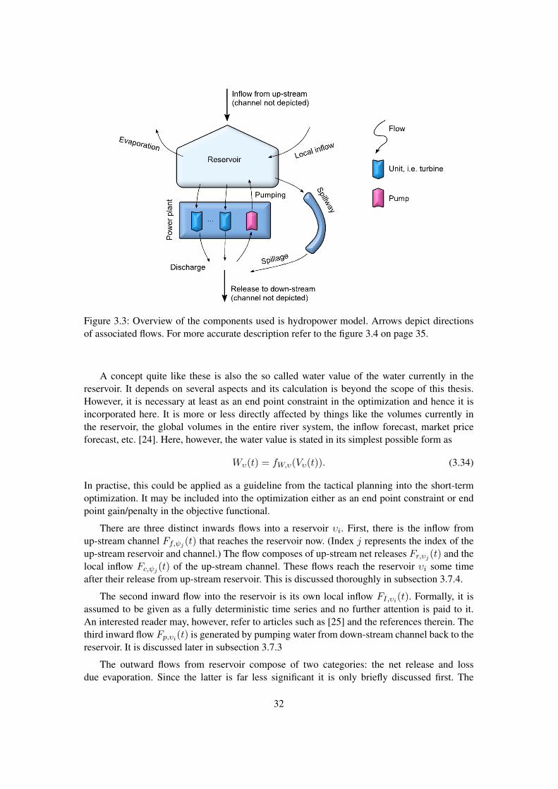
Figure 3.3: Overview of the components used is hydropower model. Arrows depict directionsof associated flows. For more accurate description refer to the figure 3.4 on page 35.

A concept quite like these is also the so called water value of the water currently in thereservoir. It depends on several aspects and its calculation is beyond the scope of this thesis.However, it is necessary at least as an end point constraint in the optimization and hence it isincorporated here. It is more or less directly affected by things like the volumes currently inthe reservoir, the global volumes in the entire river system, the inflow forecast, market priceforecast, etc. [24]. Here, however, the water value is stated in its simplest possible form as

Wυ(t) = fW,υ(Vυ(t)). (3.34)

In practise, this could be applied as a guideline from the tactical planning into the short-termoptimization. It may be included into the optimization either as an end point constraint or endpoint gain/penalty in the objective functional.

There are three distinct inwards flows into a reservoir υi. First, there is the inflow fromup-stream channel Ff,ψj

(t) that reaches the reservoir now. (Index j represents the index of theup-stream reservoir and channel.) The flow composes of up-stream net releases Fr,υj (t) and thelocal inflow Fc,ψj

(t) of the up-stream channel. These flows reach the reservoir υi some timeafter their release from up-stream reservoir. This is discussed thoroughly in subsection 3.7.4.

The second inward flow into the reservoir is its own local inflow FI,υi(t). Formally, it isassumed to be given as a fully deterministic time series and no further attention is paid to it.An interested reader may, however, refer to articles such as [25] and the references therein. Thethird inward flow Fp,υi(t) is generated by pumping water from down-stream channel back to thereservoir. It is discussed later in subsection 3.7.3

The outward flows from reservoir compose of two categories: the net release and lossdue evaporation. Since the latter is far less significant it is only briefly discussed first. The

32

evaporation from the reservoir depends on reservoir’s surface area, current air temperature(at the reservoir) ςυi(t) and humidity κυi(t). Formally the relationship is given as Fe,υi(t) =Fe,υi(fA,υi(Vυi(t)), ςυi(t), κυi(t)).

The net release from the reservoir υi is notated as Fr,υi(t). It composes of three parts: 1)sum of all discharges, 2) spilled flow (spillage) and 3) pumping back to reservoir. The last onehas an opposite direction compared to others.

Discharge of unit ωi unit is notated by δωi(t). Hence the total discharge of the plant πj canbe given as

∑i:ωi∈Ωπj

δωi(t), now referred to as simply∑δ(t). Practically, discharge is an ad-

justable flow; mathematically it is a decision variable. It is further discussed in subsection 3.7.3.

The second part in release is the spilled flow, i.e. spillage Fσ,υi(t). It means the flow spilledfrom the reservoir via spillway. Economically talking, spillage is always wasted energy andhence it is typically used only for regulation purposes. It is further discussed in subsection 3.7.2.

The last flow of net release has opposite direction as the previous two. Pumped flow Fp,υi(t)is included into net release for notational convenience, and is further discussed later.

Constraints in reservoir model

In addition to functional relationships and interconnections there naturally are several con-straints for parameters in the reservoir model. In the reservoir’s case the constraints are as-sociated with its level and the change rate of the level, i.e. time derivative.

There are two types of constraints for the water level in the reservoir υi. First there arethe physical hard constraints that ensure that the level stays within acceptable limits. Theseconstraints include physical limits of the system and other limits due to all the stakeholders. Nodeviation from these is allowed.

Second category of the limits are the soft constraints that are set to guide operation to staywithin recommended limits yet to allow deviations if needed. These include all sorts of limits,e.g the ones that come from tactical planning. Generally, soft limits are used for many purposesbut simultaneously to guarantee flexibility of the system. There is an associated penalty fromviolation. Typically the penalty is a function of the deviation. Here it is also assumed that thepenalty is symmetric in a sense that being under the lower limit is as bad a violation as beingsame amount on top of the upper limit. The penalties are generally denoted with b that has lowerindexes to point out the context.

The hard constraints for the water level h1(t) are here denoted as follows. A lower index h1

is used to point out that the constraint is associated with level h1 and υ to point out whichreservoir is in question. The upper index tells whether it is a lower or upper limit. Hence

h1,υi(t) ∈ [ hmin1,υi

(t) , hmax1,υi

(t) ] ∀ t and ∀ i

Explicit time dependency is used to allow limits that vary with time. If this is not the case or itis considered useless time-dependent constraints can naturally be replaced with constants.

Similarly, there are hard constraints for change rate of the water level:

h1,υi(t) ∈ [ dhmin1,υi

(t) , dhmax1,υi

(t) ] ∀ t and ∀ i

33

where letter d tells that the limit is associated with level’s derivative.

Finally, there are the soft limits; the water level —though it has a desired target range— isallowed to deviate from it somewhat. The associated penalty is considered a loss and weakensthe value of the objective functional. The dependency between magnitude of the penalty andthe deviation is given via function bh1,υi

. Notationally, the soft limits are as hard ones but anadditional symbol ∼ is added on top of them to point out that the limit is soft. The penalty fromsoft limit violations is given as

bh1,υi(t) =

bh1,υi

(hmin1,υi

(t)− h1,υi(t)), h1,υi(t) < hmin1,υi

(t);0, hmin

1,υi(t) ≤ h1,υi(t) ≤ hmax

1,υi(t);

bh1,υi(h1,υi(t)− hmax

1,υi(t)), h1,υi(t) > hmax

1,υi(t);

where naturally hmin1,υi

(t) < hmin1,υi

(t) < hmax1,υi

(t) < hmax1,υi

(t).

Run-of-the-river cases

In the context of reservoir it is natural to briefly discuss so called run-of-the-river cases. Itrefers to cases where there practically is no reservoir in front of the power plant and thus thetotal release through the plant equals the incoming flow from the up-stream river. The modeldeveloped here can incorporate such cases in two ways. The first and most straightforwardmethod is to simply introduce an additional constraint that forces the net release to equal theinflow. In such case, this is merely an additional constraint on the decision variables.

Another way is simply to introduce a sort of a virtual reservoir whose properties guaranteethat there is no practical possibility to store water: both the water level as a function of reservoirvolume and the constraints for the level are set so that it is not possible to let the net releasesignificantly deviate from inflow.

3.7.2 Channel and spillway models

Channels bind reservoirs together. Once the water has been released from a reservoir it flowswithin a channel to next reservoir; generally, there always is one channel for one reservoir.Hence, channels inherit reservoirs index, i.e. the channel originating from reservoir υi is notatedby ψi.

There are two types of inflows into the channel ψi: 1) the net release from up-stream reser-voir υi and 2) channel’s own local inflow Fc,ψi

(t). The latter is treated here similarly as reser-voir’s local inflow, i.e. it is assumed to be fully deterministic time series. The net release intothe channel, on the other hand, is specified in the previous subsection 3.7.1. Correspondingly,the only outward flow related to channel is a part of the net release, i.e. pumped flow. See 3.7.1and 3.7.3.

The flow within channel ψi is referred to as Ff,ψi(t). It is the sum of net release and chan-

nels local inflow Fr,υi(t) + Fc,ψi(t). Now, consider a river with a known area of cross-section,

velocity and flow. An increase in flow results in an increase either in the area of cross-section orvelocity — or practically both. In practice, the first means that the surface level of the river rises.In this thesis it is assumed that rivers have constant velocity (reasoning for this can be found from

34

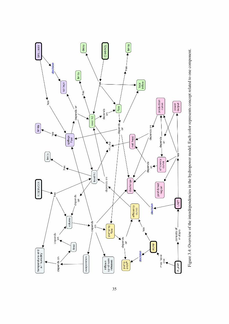
Figu

re3.

4:O

verv

iew

ofth

ein

terd

epen

denc

ies

inth

ehy

drop

ower

mod

el.E

ach

colo

rrep

rese

nts

conc

eptr

elat

edto

one

com

pone

nt.

35

the end of this subsection 3.7.2). Hence, increase in flow results in increase in channel’s level h2.Channel’s level may, however, be also dependent on the surface level of the following reservoir.This case is particularly important when the channel combining two reservoirs is either veryshort or purely virtual. In addition, the flow components (net release and local inflow) are givenan option to have different effects.

The functional form of the relationship between channel’s flow and its level is then given as

h2,ψi(t) = fh2,ψi

(Fr,υi(t), Fc,ψi(t), h1,υj (t))

Since there are no dynamic features in this approximation one must be careful with the magni-tude of the changes that this introduces into level h2. This approximation is one of the weakestpoints in the present model, yet its effects are considered minor. It is introduced in the first placeto allow the incorporation of effect of tail water level into power production via net head.

Another property that channels have is the delay they introduce to the model. Since the riversdo have a finite length and velocity they also introduce delays in the flows between the reservoirs.Since no interest is paid for length or velocity in this work, their contribution is incorporated viadelays. Generally, delay due to channel ψi is denoted byDψi

. See the reasoning behind assumedconstant delays at the end of this subsection.

A spillway is an object quite similar to a channel. On the other hand it is simpler, on theother their flow is adjustable. The decision variable συi(t) ∈ [0, 1] is set by the decision makerand it results in spillage flow Fσ,υi(t). The resulting flow, however, may be dependent both onreservoir’s water level h1,υi(t) and channel’s water level h2,ψi

(t). This relationship is given as

Fσ,υi(t) = Fσ,υi(συi(t), h1,υi(t), h2,ψi(t)).

Whether or not the tail water level plays any role is case-specific.

Reasoning behind assumed constant delays

The reasoning behind assumed constant delays —and equally constant river velocities— lieswithin the structure of the system equations presented in subsection 3.7.4 (see eq. (3.36) onpage 41). As a counter example consider flow-dependent channel delays Dψi

(Ff,ψi) and net

release Fr,υi(t1) at time t1. The flow will reach the following reservoir after time Dψi(Ff,ψi

),i.e. at some time t3 > t1. Hence, the delay can be seen as a mapping from release time t1to some time in future t3. This mapping, however, is not one-to-one mapping (bijection) sincedepending on the flow it is possible that flow released at some other time t2: t1 < t2 < t3 mightreach the next reservoir also at time t3. This poses a problem in system equation when trying tolist the flows from the up-stream channel that reach the reservoir at some time t. It is naturallypossible to overcome this problem but in this context it is not considered worth the resultingcomplications in the model.

Constraints in channel and spillway models

As with reservoir model (the previous subsection 3.7.1) there are both hard and soft constraintsin the channel model, too. For spillway there are only hard limits for its flow.

36

The hard constraints for the channel’s flow Ff,ψi(t) are

Ff,ψi(t) ∈ [ Fmin

f,ψi(t) , Fmax

f,ψi(t) ] ∀ t and ∀ i.

The soft limits for the flow are expressed as in previous sections and the penalty for its violationis given as

bFf ,ψi(t) =

bFf ,ψi

(Fminf,ψi

(t)− Ff,ψi(t)), Ff,ψi

(t) < Fminf,ψi

(t);0, Fmin

f,ψi(t) ≤ Ff,ψi

(t) ≤ Fmaxf,ψi

(t);bFf ,ψi

(Ff,ψi(t)− Fmax

f,ψi(t)), Ff,ψi

(t) > Fmaxf,ψi

(t);

where Fminf,ψi

(t) < Fminf,ψi

(t) < Fmaxf,ψi

(t) < Fmaxf,ψi

(t). Similarly, the hard constraints for the changerate of the flow are

Ff,ψi(t) ∈ [ dFmin

f,ψi(t) , dFmax

f,ψi(t) ] ∀ t and ∀ i.

Furthermore, there naturally are hard limits for channel level h2:

h2,ψi(t) ∈ [ hmin

2,ψi(t) , hmax

2,ψi(t) ] ∀ t and ∀ i

and similarly for the spillage Fσ,υi :

Fσ,υi(t) ∈ [ Fminσ,υi

(t) , Fmaxσ,υi

(t) ] ∀ t and ∀ i.

Converging/branching rivers

Although the developed model implicitly assumes that there is only one channel per reservoirit is possible to include also cases where two rivers starting from different reservoirs converge.In case of converging rivers there simply is an own set of constraints for the joint river part: inaddition to constraints of each river alone, the joint river has to fulfil its own requirements. Inpractice this means that there are constraints for the sum of the flows in distinct rivers.

3.7.3 Unit and plant models

Formally, a plant is merely a collection of units. Hierarchically, also the pump is associated witha plant. In practice, however, there are limitations to entire plants and thus they are treated asentities instead of merely a set of units (see the end of this subsection).

In the hydropower context here a unit is synonym to a turbine. Units are the componentsthat generate economical income. This income —in addition to market price s(t), naturally—depends on power output Pω(t) of the unit. The power output, on its behalf, depends on dis-charge flow δω(t) through the unit via some specific functional relationship. Naturally, poweroutput also depends on unit’s current efficiency.

Since the discharge flow δω(t) is treated as a decision variable the power output can begiven using the two following functions. In addition to discharge also the net head (differencebetween reservoir’s and down-stream channel’s level) hπi(t) = h1,υi(t) − h2,ψi

(t) affects the

37

output. Hierarchically, net head is considered a plant property. The production and efficiencyfunctions are

production function : fprod,ωi(δωi(t), hπi(t))

andefficiency function : feff,ωi(δωi(t), hπi(t))

With these the power output can be given as

Pωi(t) = fprod,ωi(δωi(t), hπi(t)) · feff,ωi(δωi(t), hπi(t))

A plant may have a pump used to pump water back to reservoir from down-stream channel.The pump is associated with the plant and it is assumed to have a constant power Ppump,πi . Thusthe flow it generates Fp,πi(t) depends on the water levels within the channel and reservoir. Thedecision related to the pump is simply whether it is on or off; the pump decision is ηπi(t) ∈0, 1. Functionally, the pumped flow is given by

Fp,πi(t) = ηπi(t) · fp,πi(h1,υi(t), h2,ψi(t)).

Constraints in plant and unit models

Physical transmission restrictions set hard constraints for the total power output of power plants.Defining the total power output of plant πj as

Pπj (t) ≡∑

i:ωi∈Ωπj

Pωi(t)

the constraints can be expressed compactly as

Pπj (t) ∈ [ Pminπj

(t), Pmaxπj

(t) ] ∀ t and ∀ j.

Since discharge is directly a decision variable of the system the constraints affecting it aredirect control constraints. Like with most of the constraints there are both soft and hard limitsin this context, too. Briefly —as in the previous cases— the hard physical constraints for bothdischarge and its change rate can be expressed as

δωi(t) ∈ [ δminωi

(t), δmaxωi

(t) ]

andδωi(t) ∈ [ dδmin

ωi(t), dδmax

ωi(t) ]

The discharge constraints, however, are more complex than those of other variables. Yi [3]has considered a case where these so called prohibited operation regions of turbines —regionswhere physical phenomena such as cavitation and resonances limit the acceptable operationregion— are given on power output vs. net head plane (using notation adopted here in (Pω, hπ)-plane). See figure 3.5 for an example used by Yi. Now, since on a given net head hπj there isa mapping from discharge flow to power output the representation used by Yi can be translatedinto a similar constrained region on (δω, hπ)-plane. Practically, this means that the allowedregions for discharge depend on the current net head hπj .

38

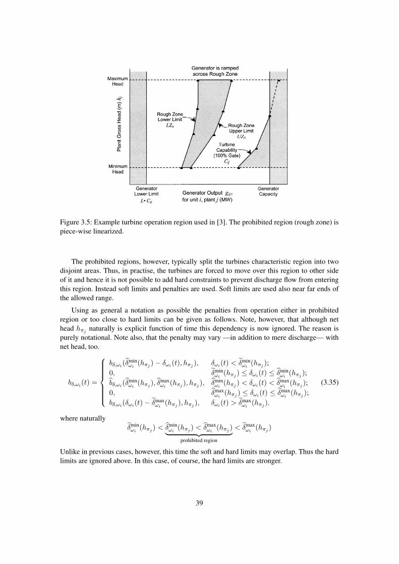
Figure 3.5: Example turbine operation region used in [3]. The prohibited region (rough zone) ispiece-wise linearized.

The prohibited regions, however, typically split the turbines characteristic region into twodisjoint areas. Thus, in practise, the turbines are forced to move over this region to other sideof it and hence it is not possible to add hard constraints to prevent discharge flow from enteringthis region. Instead soft limits and penalties are used. Soft limits are used also near far ends ofthe allowed range.

Using as general a notation as possible the penalties from operation either in prohibitedregion or too close to hard limits can be given as follows. Note, however, that although nethead hπj naturally is explicit function of time this dependency is now ignored. The reason ispurely notational. Note also, that the penalty may vary —in addition to mere discharge— withnet head, too.

bδ,ωi(t) =

bδ,ωi(δminωi

(hπj )− δωi(t), hπj ), δωi(t) < δminωi

(hπj );0, δmin

ωi(hπj ) ≤ δωi(t) ≤ δmin

ωi(hπj );

bδ,ωi(δminωi

(hπj ), δmaxωi

(hπj ), hπj ), δminωi

(hπj ) < δωi(t) < δmaxωi

(hπj );0, δmax

ωi(hπj ) ≤ δωi(t) ≤ δmax

ωi(hπj );

bδ,ωi(δωi(t)− δmax

ωi(hπj ), hπj ), δωi(t) > δmax

ωi(hπj ).

(3.35)

where naturallyδminωi

(hπj ) < δminωi

(hπj ) < δmaxωi

(hπj )︸ ︷︷ ︸prohibited region

< δmaxωi

(hπj )

Unlike in previous cases, however, this time the soft and hard limits may overlap. Thus the hardlimits are ignored above. In this case, of course, the hard limits are stronger.

39

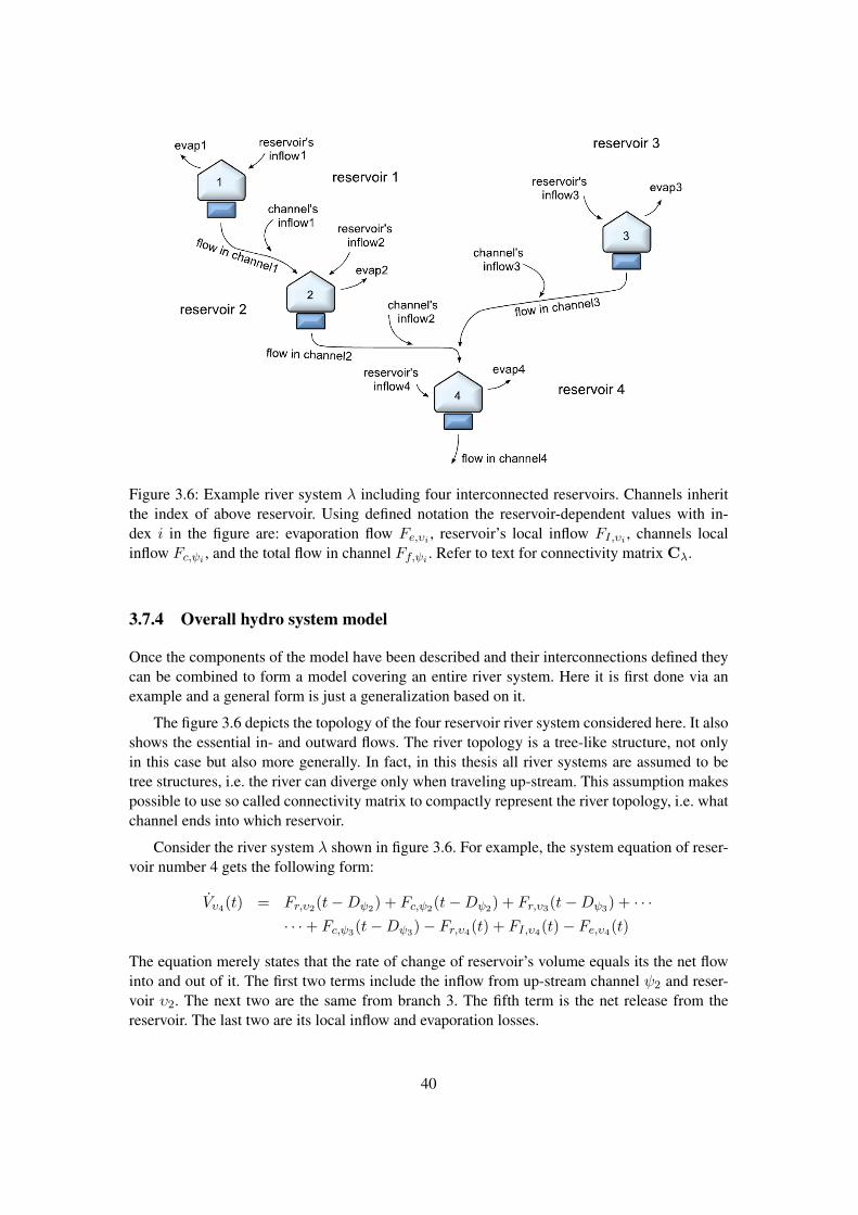
Figure 3.6: Example river system λ including four interconnected reservoirs. Channels inheritthe index of above reservoir. Using defined notation the reservoir-dependent values with in-dex i in the figure are: evaporation flow Fe,υi , reservoir’s local inflow FI,υi , channels localinflow Fc,ψi

, and the total flow in channel Ff,ψi. Refer to text for connectivity matrix Cλ.

3.7.4 Overall hydro system model

Once the components of the model have been described and their interconnections defined theycan be combined to form a model covering an entire river system. Here it is first done via anexample and a general form is just a generalization based on it.

The figure 3.6 depicts the topology of the four reservoir river system considered here. It alsoshows the essential in- and outward flows. The river topology is a tree-like structure, not onlyin this case but also more generally. In fact, in this thesis all river systems are assumed to betree structures, i.e. the river can diverge only when traveling up-stream. This assumption makespossible to use so called connectivity matrix to compactly represent the river topology, i.e. whatchannel ends into which reservoir.

Consider the river system λ shown in figure 3.6. For example, the system equation of reser-voir number 4 gets the following form:

Vυ4(t) = Fr,υ2(t−Dψ2) + Fc,ψ2(t−Dψ2) + Fr,υ3(t−Dψ3) + · · ·· · ·+ Fc,ψ3(t−Dψ3)− Fr,υ4(t) + FI,υ4(t)− Fe,υ4(t)

The equation merely states that the rate of change of reservoir’s volume equals its the net flowinto and out of it. The first two terms include the inflow from up-stream channel ψ2 and reser-voir υ2. The next two are the same from branch 3. The fifth term is the net release from thereservoir. The last two are its local inflow and evaporation losses.

40

Rather generally, the balance of a single reservoir υi can be expressed as a sum of threeterms:

Vυi(t) =∑j

Fr+c,υj (t−Dψj)− Fr,υi(t) + FI,e,υi(t)

The first term represents sum of all inflows from up-stream channel that reach the reservoir υiat time t, i.e. channel-dependent time Dψj

after release from up-stream reservoir υj . Note, thatalso local inflows of the interconnecting channels are incorporated and they are also delayed.This is done for notational convenience and has no further implications than a need to shiftchannel’s inflow by some channel-dependent amount. Index j is used merely to point out theup-stream channels that end into reservoir υi. The second term includes current net release fromthe reservoir. The last term includes both the reservoir’s local inflow and evaporation losses. Theused notation will become evident shortly.

The number of above system equations is equal to the number of reservoirs in the riversystem. Expression of the system equations of a large system would thus turn out to be ratherspace consuming. Introducing a so called connectivity matrix Cλ for river system λ makes thepresentation more compact. The idea of connectivity matrix is taken from [5] but it is applied indifferent and more complex setting.

Now, considering river system λ in figure 3.6 define a vector Vλ(t) = [V1 V2 V3 V4]>

containing the volumes of each reservoir. Naturally then Vλ(t) = [V1 V2 V3 V4]>. Further-more, define vectors

Fr,λ(t) =

Fr,υ1(t)Fr,υ2(t)Fr,υ3(t)Fr,υ4(t)

FI,e,λ(t) =

FI,υ1(t)− Fe,υ1(t)FI,υ2(t)− Fe,υ2(t)FI,υ3(t)− Fe,υ3(t)FI,υ4(t)− Fe,υ4(t)

The first one includes all releases from every reservoir at time t. Correspondingly, the secondincludes each reservoir’s net flow due to local inflow and evaporation. Next, define vector

Fr+c,λ(t−Dψ) =

Fr,υ1(t−Dψ1) + Fc,ψ1(t−Dψ1)Fr,υ2(t−Dψ2) + Fc,ψ2(t−Dψ2)Fr,υ3(t−Dψ3) + Fc,ψ3(t−Dψ3)Fr,υ4(t−Dψ4) + Fc,ψ4(t−Dψ4)

which includes the total flows within channels delayed by each channel’s inherent delay param-eter Dψi

.

Finally, define a river system-dependent connectivity matrix Cλ ∈ R4×4. In this case it takesthe following form

Cλ =

1

1 1

Now, the system equations of the river system in figure 3.6 can be expressed briefly as

Vλ(t) = Cλ · Fr+c,λ(t−Dψ)− I · Fr,λ(t) + FI,e,λ(t), (3.36)

where I is an identity matrix ∈ R4×4.

41

In addition to this, also the initial states of the state variables are naturally needed:

Vλ(t = 0) = V0,λ. (3.37)

Generally, the above equation (3.36) with river system-specific connectivity matrix Cλ givesa general characterization of the dynamics of an entire river system. The representation is com-pact, yet extensive.

3.7.5 Hydropower optimization sub-problem

In this section an objective functional for the hydropower optimization sub-problem is formu-lated. Barros has given several possible objective formulations of possible objective functionsand functional for independent hydropower optimization sub-problem [4]. In this case only onespecial form is considered, namely the market value of the production over some given time in-terval. However, things are a bit more complicated for also the possibility that production plantsalong the run of the entire river system may belong to different balance areas.

Consider the river system λ, the balance/price area ξ, the reservoir υ, the associated plant π,and the unit ω. The set of units of the plant π is Ωπ. Similarly, the set of the reservoirs withinthe river system λ is denoted by Υλ. Furthermore, the set of balance/price areas over which theriver system λ spans is denoted by Ξλ.

The power output of the unit ω belonging to the plant π is given by the function

Pω(t) = feff(δω(t), hπ(t)) · fprod(δω(t), hπ(t)).

The net power output of the plant π is the sum of outputs of its units subtracted by the (constant)power of its pump Ppump,π, i.e:

Pπ(t) =∑ω∈Ωπ

Pω(t)− ηπ(t) · Ppump,π

Next, consider the balance area ξ. The set of plants that simultaneously belong to bothbalance area ξ and the river system λ is denoted by Πλ∩ξ. The instantaneous net power outputof the plants of the river system λ that belong to the balance area ξ equals to∑

π∈Πλ∩ξ

Pπ(t).

Thus, the overall market value of the power output from the river system λ over the time intervalt ∈ [ t1, t2 ] is ∫ t2

t1

∑ξ∈Ξλ

sξ(t)

∑π∈Πλ∩ξ

Pπ(t)

dt (3.38)

However, more common situation — especially in Nordic power markets — is that all theplant along one river system belong to one single balance area. In such cases the above notationreduces to summation over all the plants that belong to river system λ, i.e∫ t2

t1

sξ(t)

∑π∈Πλ

Pπ(t)

dt

42

In addition to the mere market value of the production (eq. (3.38)), the objective functionalhas to include also the following two terms:

1. Penalties from violations of the soft limits

2. End value terms for value at the end of the considered time period

The first ones are discussed along the model formulation. They are used either as concretepenalties or as a method to drive the optimal policies towards more suitable directions. Theend values, however, play important role in preventing the optimization from short-sightedlyutilizing all the scarce resources during the optimization time interval.

In hydropower context the term including the penalties from the soft limits violations con-sists of the following parts:

1. levels in the reservoirs bh1,υ

2. flows in the channels bFf ,ψ

3. the rough zones of the turbines bδ,ω

Together they form the following term for the entire river system λ over the optimization timeinterval

bλ =∫ t2

t1

∑υ∈Υλ

bh1,υ(t) +∑ψ∈Ψλ

bFf ,ψ(t) +∑ω∈Ωλ

bδ,ω(t)

dt (3.39)

The end values, on the other hand, compose only of the water values within each reservoirat the end of the optimization time period t2, see eq (3.34). For the river system λ this term getsthe form ∑

υ∈Υλ

Wυ(t2) (3.40)

This — together with the market value (3.38) and the penalties (3.39) — form the overall ob-jective functional for the hydropower sub-problem

∫ t2

t1

∑ξ∈Ξλ

sξ(t)

∑π∈Πλ∩ξ

Pπ(t)

dt+ bλ +∑υ∈Υλ

Wυ(t2) (3.41)

3.8 Overall model and problem formulation

The description of the focal parts of the model is given in the previous sections 3.2 through 3.7.In this section these are combined into an extensive overall procurement planning problem.

The objective function(al) is as essential as the model of the system itself. In this case theobjective functional has to incorporate information about the following aspects:

1. Market price

43

2. Own production

3. Contractual position

4. Cost of procurement

5. Start-up costs

6. Penalties

7. End values

In addition to these the objective functional has to be able to take into account all the possibleroles the BR may occupy. Practically speaking, this means that the possibility of both the positiveand negative contractual positions has to be included.

A natural assumption at this point is that the money associated with the agreed contracts hasalready changed hands. Thus the objective is simply to maximize the market value of BR’s ownproduction. Consider a single price area and the following term

s(t)× [P (t)− C(t)] , (3.42)

where P (t) stands for the total own production within the price area under consideration.Equally, C(t) is used to denote the net contractual position within the price area. Now, thereare three distinct cases:

P(t)=C(t) Own production equals the contractual position. In this case no trade takes place atthis time and hence the there is no power to be sold to markets. Thus, there is no income.This is the case in after-spot situation because there is no possibility to participate in thetrading anymore1.

P(t)>C(t) Own production is greater that the contractual position. The excess power is sold inthe exchange at the current market price. The amount of this power is P (t)−C(t) and itsmarket value naturally is s(t)[P (t)− C(t)]

P(t)<C(t) Own production is less than the contractual position. To meet the obligations the BRhas to buy the missing power C(t)− P (t) from the exchange at the current market price.

With these it become evident that eq. (3.42) fully characterizes the different aspects of BR’sroles.

The incorporation of the costs of own production is straightforward. Denoting the total costof production within one price area by c(t) one can write the objective functional as

s(t)× [P (t)− C(t)]− c(t). (3.43)

Now, only the start-up costs, penalties and the end values are missing. They are naturallyassumed to commensurable and hence merely added at the end of the equation.

1This is a drastic simplification: in real life there naturally is is a possibility to participate in ELBAS trading andboth balance and regulation energy markets. However, in this model these alternatives are not included.

44

The end values concern the state variables of the system, i.e. reservoir volumes Vλ(t) ∀λand heat accumulator charges qh(t) ∀H. In addition to these there also are the unit status profilebinaries uω(t) but no end values are associated with them. Similarly, in this case no end valuesare associated with heat accumulators, either. Thus the end values incorporated in this case arethe water values within reservoirs, see eq. (3.40).

Hence, the overall procurement planning objective functional is the time integral over sum ofthe unit-wise equations (3.43) over the price areas added with the end state costs and subtractedby the penalties and start-up costs:∫ t2

t1

∑ξ∈Ξ

sξ(t)× [Pξ(t)− Cξ(t)]− cξ(t) dt + · · ·

· · ·+∑ω∈Ω

cs,ω(uω(t)) +∑υ∈Υ

Wυ(t2) −∑λ∈Λ

bλ (3.44)

The last penalty term is originally presented on page 43 (eq. (3.39)).

The set of the decision variables in the problem is denoted by D. It consists of the followingvariables:

1. Convex combination coefficients per unitvi(t), wi,j(t)ni

j=1

mω

i=1∀ ω ∈ Ω

2. Unit status profile uω(t) ∀ ω ∈ Ω

3. Discharge per hydro unit δω(t) ∀ ω ∈ Ω

4. Spillage per hydro plant σπ(t) ∀ π ∈ Π

5. Pumping per hydro plant ηπ(t) ∀ π ∈ Π

6. Usage per procurement contract Cp,φ(t) ∀ φ ∈ Φ

7. Heat accumulator input qA,h(t) ∀ h ∈ H

This seamlessly applies to the after-spot situation also because once no trading is possible (i.e.P (t) = C(t)) the functional reduces to cost minimization

maxD

∫ ∑ξ∈Ξ

sξ(t)× 0− cξ(t) dt = minD

∫ ∑ξ∈Ξ

cξ(t) dt (3.45)

With the objectives functional, the constraints and the above in mind it is obvious that the result-ing overall procurement planning problem is a rather complex example of what generally knownas non-linear, non-convex, highly dynamical MIP. Practically, it contains all the difficult char-acteristics that an optimization problem can [26]. As such, it would easily be characterized hardif not practically impossible. Hard solution time constraints require substantial approximations.The summary of the overall planning problem is presented in the appendixes, see appendix A.

45

3.9 Model simplifications and assumptions

Simplifications and assumptions that affect the scope of the plausible domain of the model arelisted below2 .

Generalized CHP plants The condense power plants and heat sources are modeled as specialcases of a general CHP model. The most general unit model in this thesis is that of CHPunit. It is modeling via partially convex characteristic area and thus leads essentially toMIP problem.

Only two commodity balances included No steam or fuel balance have been included, onlytwo commodity plants and balances have been modeled. Addition of more complex com-modity characteristics requires changes of the model.

No trading or transfers between balances Balances do not interact with each other in anyother ways than possibly via exchange prices that affect prices on other price areas, too.Neither inter-balance trading nor transmissions are possible. However, the different areaprices should effectively eliminate the need for these aspects.

No after-spot trading or regulation power The possibility for e.g. ELBAS trading has notbeen included; the after-spot trading is not possible. The regulation power reservoir andtheir valuation have not been included. However, their incorporation into the model wouldhave been difficult and its value questionable.

Unit status changes no adequately included in the optimization model The formulated op-timization problem does not readily include unit status change model. Its model has beenseparately incorporated to ensure that its information needs will be fulfilled.

Simple channel model Channels are modeled as collective units and do not include furtherriver properties. In addition, the hydropower model assumes that there are constant, flow-independent delays that the channels introduce. The lack of flow-delay dependence maylimit the validity of the model.

Of these the first three ones are the most restricting; there are several cases where two commod-ity model combined with simple one unit plant model are not capable of incorporating relevantproperties of the modeled plants. For example, plants with multiple different steam sources andbalances pose problems on the chosen model. However, with appropriate mathematical modelthe information modeling and resulting conceptual schemas of such systems can be quite easilyformulated. In some real world cases also the inability to count for the transfer between balancesmay introduce unnecessary inflexibility to the model.

2The critical simplification of the modeling approach also was that all the forecasts were treated as fully deter-ministic and no stochastic characteristics at were incorporated into the model. However, this is not included into thelist below for it is more of an inherent property of the chosen approach than simply an approximation of the model.

46

Chapter 4

Information model of procurementplanning problem

In this chapter the components of the mathematical procurement planning model are turned intoconceptually distinct entities. They are identified and given descriptive names; this correspondsto creating an ontology on this domain. Similarly, relationships of these entities are identified.Together the entities and relationships result in a conceptual schema that covers this domain.The conceptual schema as such is rather close to the actual information model; the difference isthat instead of composing of abstracts concepts the information model is a concrete instance —a concretization — of its conceptual schema.

The figure 4.1 offers a summarizing overview of the process and the concepts. It depicts thefocal concepts and their interconnections. The starting point for these is the mathematical modelof the procurement planning problem formulated in the previous chapter. The enumerated stepsin the figure are discussed in the following:

1. Conceptually distinct entities of the mathematical model are identified and named, that is,ontology on this domain is created.

2. Relationships of the mathematical model are identified and named. In this case all therelationships will turn out to be either is-part-of or belongs-to relations.

3. Together the ontology and the relations constitute the overall conceptual schema of theprocurement planning problem. Also the representation method has to be fixed here.

4. Once the user configures the model, i.e. fixes the free parameters of the model all theentities become concrete instances of the abstracts concepts defined in the previous step.

5. The information model is the concretization of the conceptual schema, i.e. its instance.

6. Interface is the concrete instance of the information model, e.g an XML rendered repre-sentation of the information model

The first step on the way is to identify the conceptually distinct entities and name them. Thiscorresponds to creating an ontology, which can be defined as follows:

47

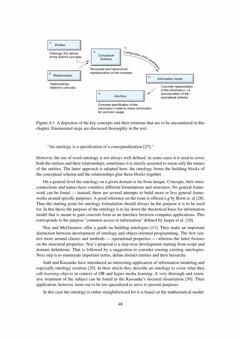
Figure 4.1: A depiction of the key concepts and their relations that are to be encountered in thischapter. Enumerated steps are discussed thoroughly in the text.

"An ontology is a specification of a conceptualization [27]."

However, the use of word ontology is not always well defined: in some cases it is used to coverboth the entities and their relationships, sometimes it is strictly assumed to mean only the namesof the entities. The latter approach is adopted here; the ontology forms the building blocks ofthe conceptual schema and the relationships glue these blocks together.

On a general level the ontology on a given domain is far from unique. Concepts, their inter-connections and names have countless different formulations and structures. No general frame-work can be found — instead, there are several attempts to build more or less general frame-works around specific purposes. A good reference on the issue is offered e.g by Borst et. al [28].Thus the starting point for ontology formulation should always be the purpose it is to be usedfor. In this thesis the purpose of the ontology is to lay down the theoretical basis for informationmodel that is meant to gain concrete form as an interface between computer applications. Thiscorresponds to the purpose "common access to information" defined by Jasper et al. [10].

Noy and McGuinness offer a guide on building ontologies [11]. They make an importantdistinction between development of ontology and object-oriented programming. The first cen-ters more around classes and methods — operational properties — whereas the latter focuseson the structural properties. Noy’s proposal is a step-wise development starting from scope anddomain definitions. That is followed by a suggestion to consider reusing existing ontologies.Next step is to enumerate important terms, define distinct entities and their hierarchy.

Suhl and Kassanke have introduced an interesting application of information modeling andespecially ontology creation [29]. In their article they describe an ontology to cover what theycall learning objects in context of OR and hyper media learning. A very thorough and exten-sive treatment of the subject can be found in the Kassanke’s doctoral dissertation [30]. Theirapplication, however, turns out to be too specialized to serve to present purposes.

In this case the ontology is rather straightforward for it is based on the mathematical model.

48

The names given to the model components in the previous chapter can be used rather easily inthis context, too. Only minor changes will be introduced. Following Noy’s guidelines the firstnatural step is the identification and fixing of the component names. The specific properties ofthe relationships are discussed nearly simultaneously.

In this chapter first a general overview of the widespread information modeling methodcalled Entity-Relationship (ER) model is offered. In the same context XML and MathML for-mats are also briefly discussed. The idea is to show that the combination of these formats andthe ER-based information model/conceptual schema is suitable choice for the interface once aproper tagging (naming) is introduced. In fact, the ER model turns out to be even too sophisti-cated and is in this thesis actually reduced to a subset of the original method.

After the general discussion covering the theoretical aspects of the information modeling theontological needs of the problem are discussed. The main emphasis is on the special purposeat hand in this thesis: the interface to transmit the parametric information between computerapplications. Also an overview of possible ways to represent the finding in a graphical and textformats is included. This is followed by descriptions of the entities and their relationships, i.e.the actual schema of the domain. The representation methods discussed earlier are used here.A distinction between abstract mathematical and more concrete model entities is made and thediscussion proceeds following this idea.

4.1 Theoretical overview of the information modeling

4.1.1 Chen’s ER model

There are several ways to define and structure conceptual schemas and information models.The used terminology is not very accurate and the terms are sometimes used interchangeably.In this thesis the definitions given in the previous introduction are followed. In this section theso-called Entity-Relationship model is discussed more thoroughly; it gives a general overviewof the theories behind information modeling and is a suitable method to model both entities andrelationships. As such it results in a conceptual schema on the domain.

Edgar F. Codd and Peter Chen, among others, laid down theoretical foundations of moderninformation modeling in the 70’s. Codd wrote the fundamental article A Relational Model ofData for Large Shared Data Banks [31] that laid down the basis for relational informationmodeling. Later Chen offered more general view of the subject in his 1976 article The Entity-Relationship Model — Toward a Unified View of the Data [12]. The latter is considered thetheoretical basis of the modern UML standard, for example.

Quoting Chen, his work concentrates on the two identified levels of views of data:

1. Information concerning entities and relationships exist in our minds

2. Information structure — organization of information in which entities and relationshipsare represented by data

In practice, this separates the two levels of view of data: the first one is rather intuitive andnatural representation in our minds, the other is the first one turned into a structured model. This

49

is exactly what this thesis is about: identifying the essential concepts and their relationships andturning them into an abstract conceptual schema.

The essential aim of information models is to offer a systematic way to represent informationin such a manner that the integrity and logical structure are preserved. This naturally leads toabstract representations of entities and relationships between them. One of the original ideasin Chen’s Entity-Relationship model is to separate information about entities from informationabout relationships.

Two main categories in Chen’s work — entities and relationships — are defined as follows:

"An entity is a thing which can be distinctly identified."

"A relationship is an association among entities."

It is a matter of definition which things are seen as entities and which as relationships. Chen’sexample is marriage. It can be seen as relationship between two person-entities or as an entity.

Chen defines following concepts to back his discussion. We briefly refer them here to offer areference point for these repetitive concepts. For more accurate and extensive treatment see [12].

Entity and entity set Entity belongs to an entity set, e.g. for units ω ∈ Ω in our model. Natu-rally Ω is an entity set —set of all units— and ω is an single entity —unit— in it.

Relationship, role and relationship set Relationship set consists of all possible relationshipsbetween entities, whereas single ordered set of relationships (within relationship set) is arelationship. Role is a function that performs the relationship; using the role it is no longernecessary to use ordering in the relationships; its purpose is mainly semantic.

Attribute, value, and values set Information about entity or relationship is expressed by attribute-value pairs. Values are naturally classified into different value sets. An attribute is definedas a function mapping from either entity or relationship sets into value set or a Cartesianproduct of value sets.

In this thesis term entity refers to any distinct concept. It should not be mixed with termcomponent that refers to physical parts of both the procurement portfolio and mathematicalmodel of the problem. These are also referred to with term object. However, from now on termentity is used to refer to any conceptually distinct information bit. Also more complex thingsthat compose of entities are still entities.

Chen’s model represents a general and very extensive characterization of data representingentities and relationships. In the case of BR’s procurement planning problem the Chen’s modelis greatly simplified and is only partially utilized. Most of the relationships encountered herewill turn out to be simple inclusion relationships: entities belong-to — or are part-of — otherentities. This will become evident shortly.

Chen also introduces concept of entity keys: they are a set of attributes that can be usedto represent entities in more abstract form. Conceptually, they are related to the second levelview of information described earlier. A special case of entity keys is an entity primary key. Itis chosen so that there exists a semantically meaningful one-to-one mapping between entity setand the corresponding attribute value set. It corresponds to one single entity and can be used tosingle it out in every other context.

50

In figures 4.3 and 4.4 there are partial depictions of key entities and relationships in BR’sprocurement planning model. The depictions are only partial since the full incorporation of theentities present in the model would have resulted in rather large and complex figure. However,these figures depict the essential relationships between upper-level entities like balances andriver systems. Besides, as shown shortly, there is a better way to represent most of the relation-ships.

4.1.2 Overview of ontologies

Noy and McGuinness have discussed both the purpose of ontologies and the steps included intheir developments process [11]. The very first step is to carefully examine the purpose to whichthe ontology is to be applied. Its purpose not only points out the needs but also helps to findout the possible scope limitations that prevent wasting resources into useless aspects within theontology.

Also Jasper and Uschold have discussed the reasons for ontology creation [10]. They havepointed out the essential application fields and a noteworthy point is that the lists of both Jasperand Noy include the purpose that this thesis concentrates on. Noy puts it as follows:

"To share common understanding of the structure of information among people orsoftware agents"

whereas Jasper says it somewhat more generally:

"Common access to information: Information is required by one or more personsor computer applications, but is expressed using unfamiliar vocabulary, or in aninaccessible format. The ontology helps render the information intelligible by pro-viding a shared understanding of the terms, or by mapping between sets of terms.Benefits of this approach include inter-operability, and more effective use and reuseof knowledge resources."

Furthermore, also Uschold and Gruninger have discussed ontologies as ways to provide com-mon access to information [32]. They also offer several case studies of successful applicationsin different fields. In addition to the previously mentioned aspects Uschold divides the applica-tion fields of ontologies into three areas: 1) communications, 2) inter-operability and 3) systemsengineering. The last one covers specification, reliability and reusability. He sees ontologies as asort of inter-lingua and thus within the scope of this thesis one of the key goals to achieve usingontology is consistency and lack of ambiguity: "One of the most important roles an ontologyplays in communications is that it provides unambiguous definitions for terms used in a softwaresystem . . . [32]."

Noy’s guide to building ontologies [11] starts from scope and domain definitions. That isfollowed by a suggestion to consider reusing existing ontologies. Next step is to enumerateimportant terms, define distinct entities and their hierarchy. In this case the ontology is ratherstraightforward for it is based on the mathematical model. The names given to the model compo-nents in the previous chapter can be used rather easily in this context, too. Only minor changeswill be introduced. Following Noy’s guidelines the first natural step is the identification and

51

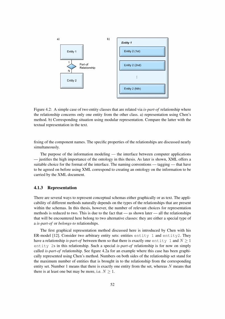
Figure 4.2: A simple case of two entity classes that are related via is-part-of relationship wherethe relationship concerns only one entity from the other class. a) representation using Chen’smethod. b) Corresponding situation using modular representation. Compare the latter with thetextual representation in the text.

fixing of the component names. The specific properties of the relationships are discussed nearlysimultaneously.

The purpose of the information modeling — the interface between computer applications— justifies the high importance of the ontology in this thesis. As later is shown, XML offers asuitable choice for the format of the interface. The naming conventions — tagging — that haveto be agreed on before using XML correspond to creating an ontology on the information to becarried by the XML document.

4.1.3 Representation

There are several ways to represent conceptual schemas either graphically or as text. The appli-cability of different methods naturally depends on the types of the relationships that are presentwithin the schemas. In this thesis, however, the number of relevant choices for representationmethods is reduced to two. This is due to the fact that — as shown later — all the relationshipsthat will be encountered here belong to two alternative classes: they are either a special type ofa is-part-of or belongs-to relationships.

The first graphical representation method discussed here is introduced by Chen with hisER-model [12]. Consider two arbitrary entity sets: entities entity 1 and entity2. Theyhave a relationship is-part-of between them so that there is exactly one entity 1 and N ≥ 1entity 2s in this relationship. Such a special is-part-of relationship is for now on simplycalled is-part-of relationship. See figure 4.2a for an example where this case has been graphi-cally represented using Chen’s method. Numbers on both sides of the relationship set stand forthe maximum number of entities that is brought in to the relationship from the correspondingentity set. Number 1 means that there is exactly one entity from the set, whereas N means thatthere is at least one but may be more, i.e. N ≥ 1.

52

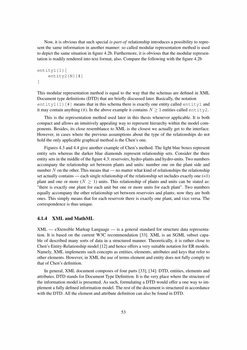
Now, it is obvious that such special is-part-of relationship introduces a possibility to repre-sent the same information in another manner: so called modular representation method is usedto depict the same situation in figure 4.2b. Furthermore, it is obvious that the modular represen-tation is readily rendered into text format, also. Compare the following with the figure 4.2b

entity11[entity2N[#]

]

This modular representation method is equal to the way that the schemas are defined in XMLDocument type definitions (DTD) that are briefly discussed later. Basically, the notationentity11[#] means that in this schema there is exactly one entity called entity1 andit may contain anything (#). In the above example it contains N ≥ 1 entities called entity2.

This is the representation method used later in this thesis whenever applicable. It is bothcompact and allows an intuitively appealing way to represent hierarchy within the model com-ponents. Besides, its close resemblance to XML is the closest we actually get to the interface.However, in cases where the previous assumptions about the type of the relationships do nothold the only applicable graphical method is the Chen’s one.

Figures 4.3 and 4.4 give another example of Chen’s method. The light blue boxes represententity sets whereas the darker blue diamonds represent relationship sets. Consider the threeentity sets in the middle of the figure 4.3: reservoirs, hydro-plants and hydro-units. Two numbersaccompany the relationship set between plants and units: number one on the plant side andnumber N on the other. This means that — no matter what kind of relationships the relationshipset actually contains — each single relationship of the relationship set includes exactly one (=1)plant and one or more (N ≥ 1) units. This relationship of plants and units can be stated as:"there is exactly one plant for each unit but one or more units for each plant". Two numbersequally accompany the other relationship set between reservoirs and plants; now they are bothones. This simply means that for each reservoir there is exactly one plant, and vice versa. Thecorrespondence is thus unique.

4.1.4 XML and MathML

XML — eXtensible Markup Language — is a general standard for structure data representa-tion. It is based on the current W3C recommendation [33]. XML is an SGML subset capa-ble of described many sorts of data in a structured manner. Theoretically, it is rather close toChen’s Entity-Relationship model [12] and hence offers a very suitable notation for ER models.Namely, XML implements such concepts as entities, elements, attributes and keys that refer toother elements. However, in XML the use of terms element and entity does not fully comply tothat of Chen’s definition.

In general, XML document composes of four parts [33], [34]: DTD, entities, elements andattributes. DTD stands for Document Type Definition. It is the very place where the structure ofthe information model is presented. As such, formulating a DTD would offer a one way to im-plement a fully defined information model. The rest of the document is structured in accordancewith the DTD. All the element and attribute definition can also be found in DTD.

53

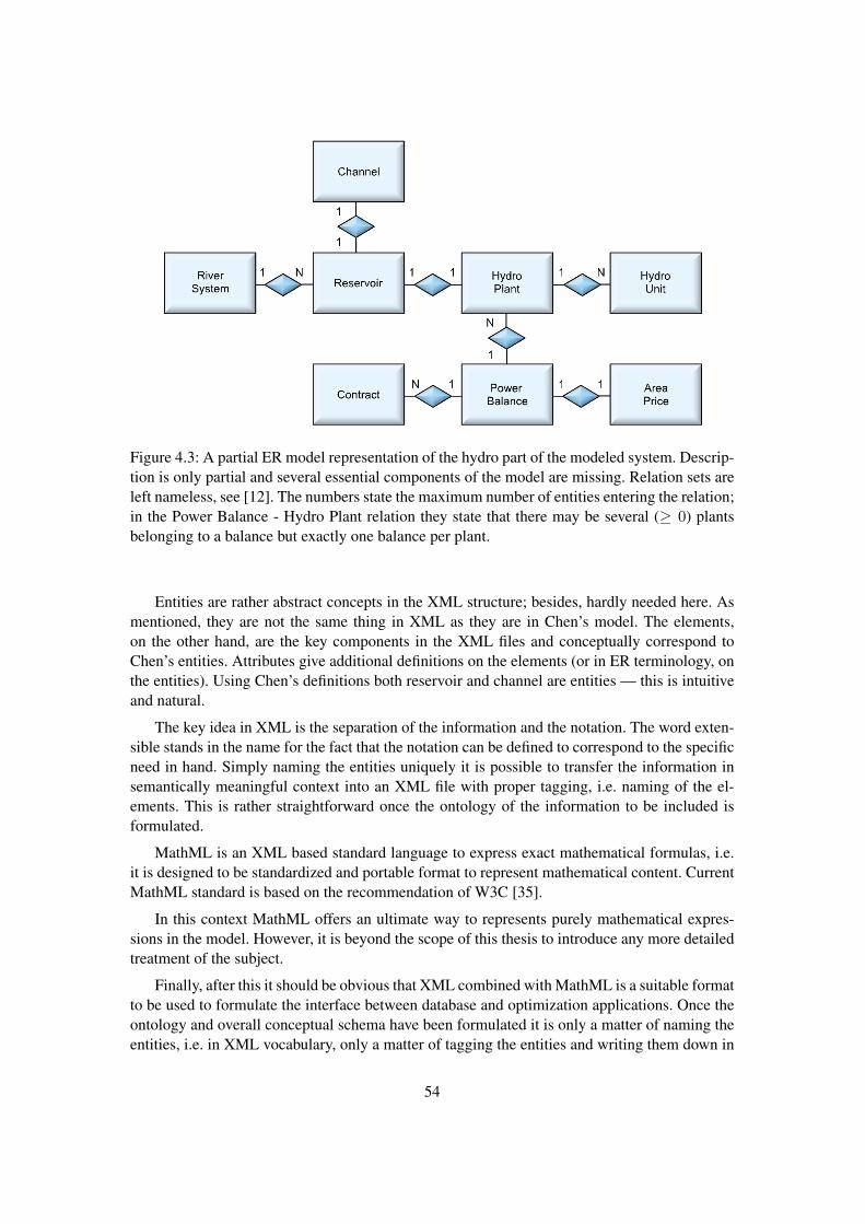
Figure 4.3: A partial ER model representation of the hydro part of the modeled system. Descrip-tion is only partial and several essential components of the model are missing. Relation sets areleft nameless, see [12]. The numbers state the maximum number of entities entering the relation;in the Power Balance - Hydro Plant relation they state that there may be several (≥ 0) plantsbelonging to a balance but exactly one balance per plant.

Entities are rather abstract concepts in the XML structure; besides, hardly needed here. Asmentioned, they are not the same thing in XML as they are in Chen’s model. The elements,on the other hand, are the key components in the XML files and conceptually correspond toChen’s entities. Attributes give additional definitions on the elements (or in ER terminology, onthe entities). Using Chen’s definitions both reservoir and channel are entities — this is intuitiveand natural.

The key idea in XML is the separation of the information and the notation. The word exten-sible stands in the name for the fact that the notation can be defined to correspond to the specificneed in hand. Simply naming the entities uniquely it is possible to transfer the information insemantically meaningful context into an XML file with proper tagging, i.e. naming of the el-ements. This is rather straightforward once the ontology of the information to be included isformulated.

MathML is an XML based standard language to express exact mathematical formulas, i.e.it is designed to be standardized and portable format to represent mathematical content. CurrentMathML standard is based on the recommendation of W3C [35].

In this context MathML offers an ultimate way to represents purely mathematical expres-sions in the model. However, it is beyond the scope of this thesis to introduce any more detailedtreatment of the subject.

Finally, after this it should be obvious that XML combined with MathML is a suitable formatto be used to formulate the interface between database and optimization applications. Once theontology and overall conceptual schema have been formulated it is only a matter of naming theentities, i.e. in XML vocabulary, only a matter of tagging the entities and writing them down in

54

Figure 4.4: A partial ER model representation of the non-hydro part of the modeled system.Compare with the figure 4.3.

a XML file.

4.2 Information modeling applied to procurement planning prob-lem

4.2.1 Purpose and required scope of conceptualization

The problem specific aspects of the information modeling and ontology creation are discussed inthis section based on the rather general overview of the subject earlier. Previous research on thefield has emphasized that the starting point for the information modeling should always be thepurpose of the model [11], [10], [32]. In this thesis the emphasis and the goal of the informationmodeling are to create a conceptual schema that lays down the basis for the interface betweenprocurement support system and multiple optimization applications. That is, BR’s procurementplanning problem has rather specialized ontological needs; it is not a typical semantic ontologydiscussed by e.g. Noy [11].

There are several possible levels on which the conceptual schema could be created. Begin-ning from the most general and simultaneously most difficult, it would be desirable to createan information model to cover the procurement planning problem at its most general level as adynamic programming problem. In practice this would mean that an ontology to cover a gen-eral dynamic programming problem had to be created. This, on the other hand, would requirecreation of an exhaustive mathematical ontology, which quite easily can be identified as nearlyimpossible task. An example of attempts to build such general frameworks in specific mathe-matical areas can be found in reference [36].

Besides, there is actually no need to create such a general framework. Instead, it is rea-sonable to assume that the structure and properties of the mathematical procurement planningproblem are common knowledge and transferring merely the parametric information is ade-quate. In other words, it is assumed that both the over-level procurement support system (seefigure 1.1) and the optimization applications operate the very same model of the problem. Thedifference is simply that the optimization engines have to relax and approximate the model inorder to be able to optimize it. These relaxations and approximations naturally are modifications

55

of the original problem, but they are not known beforehand. Thus, there is no need to extendthe information modeling to cover anything more than what is required to create a parametricinterface between the applications.

Restricting the information modeling to cover merely the parametric information within theprocurement planning model is a significant scope limitation. After that the ontology creation re-duces simply to identifying conceptually distinct parametric objects of the mathematical model.This is quite readily visible from the mathematical model itself.

4.2.2 Parametric schemas: ontology and relationships

Creating an ontology based on the mathematical procurement planning problem is rather straight-forward. It culminates on simply choosing proper, semantically meaningful and — before all —unique names on the mathematical entities. Their definitions are obvious from the model itself.However, even though the scope of the transmitted information is limited to parametric compo-nents only, the ontology should cover also the context. Thus, the resulting schemas will coverthe entire mathematical model yet only the parameters have to be fixed by the user.

The case is not much different with the relationships, either. Refer to the figures 4.3 and 4.4.From them it is obvious that it is not possible to use is-part-of relationships to capture all char-acteristics of the relationships between e.g. plants, balances and river systems: each plant maysimultaneously belong to multiple over-level concepts — e.g. every CHP plan belongs to bothpower and heat balance. In these cases there is a need to define an additional relationship calledbelongs-to relationship. Such relationships cannot be represented using the modular method andinstead the mentioned figures capture the essentials of the relationships. In practice, unique en-tity keys have to be used to implement these types of relationships: unique IDs (entity key) areassigned to every party in question and other party is uniquely associated with the other one viaan ID reference.

4.2.3 Reusability of schemas

One of the aspects that all the mentioned researcher on the field have mutually emphasized isthe reusability of the schemas [11], [10], [32]. Its role plays focal part in determining whetherthe constructed ontology is suitable for a long-term maintenance. However, in the informationmodeling discussed in this thesis the reusability of the entity schemas is not of such interestas one might expect based on the literature. In the cases referred to in the previous studies theconceptual schemas and the structure of the information has been far more complex than here.In such cases the mere complexity of the domain has emphasized the need to consider widerapplicability of the results. In this case the question of reusability reduces to a question aboutclarity and re-applicability guidelines set by the constructed schemas. In case of changes in theunderlying mathematical mode there naturally emerges a need to change the interface and theontology it is based on. Most likely, the changes are due to simple additions or reductions inthe model; the structure itself will almost inevitably compose of the very same entity arc-typesthat were used previously. Thus constructing the new schemas and new ontology in accordancewith the previous ones turns out to be of greater interest that the direct reusability of the originalones. However, considering the simplicity of the schemas developed in the following sections,the importance of this topic is questionable — once the mathematical model is known, creating

56

its conceptual schema is totally case-dependent, yet likely to make use of the same basic entitiesand relationships that are discussed in this thesis.

4.3 Model component schemas

In this section the components of the BR’s procurement planning problem are modeled as dis-tinct concepts, i.e. entities. Their relationships are briefly explained and incorporated in theresulting conceptual schema. The discussion begins from the most basic and fundamental partswithin the model, i.e. the abstract mathematical primitives that the interface actually delivers.

4.3.1 Abstract model components — basic entities

There are four entities on the most basic level, i.e. four abstract model entities. They are usedas the most fundamental building blocks when constructing other, more complex entities. Theserepresent the lower granularity level in this work. As more complex structures rise from them,the level of granularity rises, too [29]. Together with the shorter acronyms that are used later torefer to them the basic entities are:

1. Scalars SCL

2. Time series TS

3. Matrixes MTRX

4. Functions FNCT

The simplest of them naturally are the mere scalar entities. They simply represent one scalarvalue. In the mathematical model they either work as such and transmit parametric scalar valueor — more commonly — are used a the most basic building blocks to make up more complexentities like time series.

The second group of the basic entities is the time series. A time series compose of twovectors, i.e. arranged sets of scalars. Whether or not the vectors themselves, too, are treated asentities, is irrelevant: it is merely a matter of format and notation. For example, if implementedusing XML format there simply has to be entity definitions for the vectors but no further atten-tion for them is required. As a brief example, adopting to XML notation for scalar values usedby Fourer [37] one could used to following element definition in XML document type definition(DTD):

time.series1[vector2[

scalarN[#]]

]

which is equal to the following part of XML DTD :

57

<!ELEMENT time.series (vector,vector)><!ELEMENT vector (el+)><!ELEMENT el (#PCDATA)>

This defines an XML element time.series as a collection of two vector elements. Eachvector element, on the other hand, is defined as a collection of one or more (+) el elements.These may contain anything; basically they are the scalar entities mentioned before.

In time series the two vectors serve different purposes. The other one, called time vector,contains the time points — or time stamps — t1, t2, . . . , tn. The other one contains the corre-sponding values of the time series v1, v2, . . . , vn. Both of them naturally are of the same length.

In addition to the two vectors each time series may optionally have specially defined in-terpolation method. It fixes the mathematical method used to interpolate the series between itsdomain values tini=1. Most simple ones are constant interpolation and linear interpolation. Thelatter one is the most natural and also easily implemented choice. The first one, on the otherhand, is useful with time series representing such quantities that do not posses continuous prop-erties — for example, it may be grounded to make this assumption concerning hourly poweroutputs of different procurement sources if the hourly consumption is like that, too.

Another time series-like set of entities in this thesis is a matrix. It plays rather minor rolebecause it is used only in one context in the mathematical model, that is, as the connectivitymatrix of a river system. Formally, matrix could be defined as a set of vectors of equal lengthor simply as a collection of scalar entities. For large and possibly sparse matrixes an alternativeXML formulation has been introduced by Fourer [37].

The last set of basic abstract entities composes of functions. Basically, they are mappingfrom one domain onto another, but in this thesis all the mappings turn out to of the form

f : Rn → R, where n ∈ N. (4.1)

Two distinct way of representing functional mappings are discussed in this thesis. In additionto them there are countless of other ways, too, but in this case it is considered sufficient to dealthese two only. The choice is due to ease of configuring such mappings. The methods are:

1. Exact mathematical expressions via MathML

2. Look-up tables with different dimensions

The first one, exact expressions via MathML, is rather straightforward: simply express the formof the relation as an exact mathematical formula and configure it into the system using somestandard notation. The benefits of this method are obvious: first, the expression is exact. Sec-ondly, if necessary, such expression can rather easily be transformed into piecewise continuous.The problems, however, are obvious, too: establishing such expression is not straightforwardand configuring it requires knowledge of the standard of representing it to the system.

The second method for representing functions via look-up tables is more flexible that it maysound like at the first place. First of all, look-up tables can be used to approximate any mappingof the form (4.1) no matter what the domain dimension n is. Secondly, look-up tables turn outto equal to piecewise linear approximations of functions given a set of domain and value points.Hence, no interpolation method has to be chosen, it inherently is linear.

58

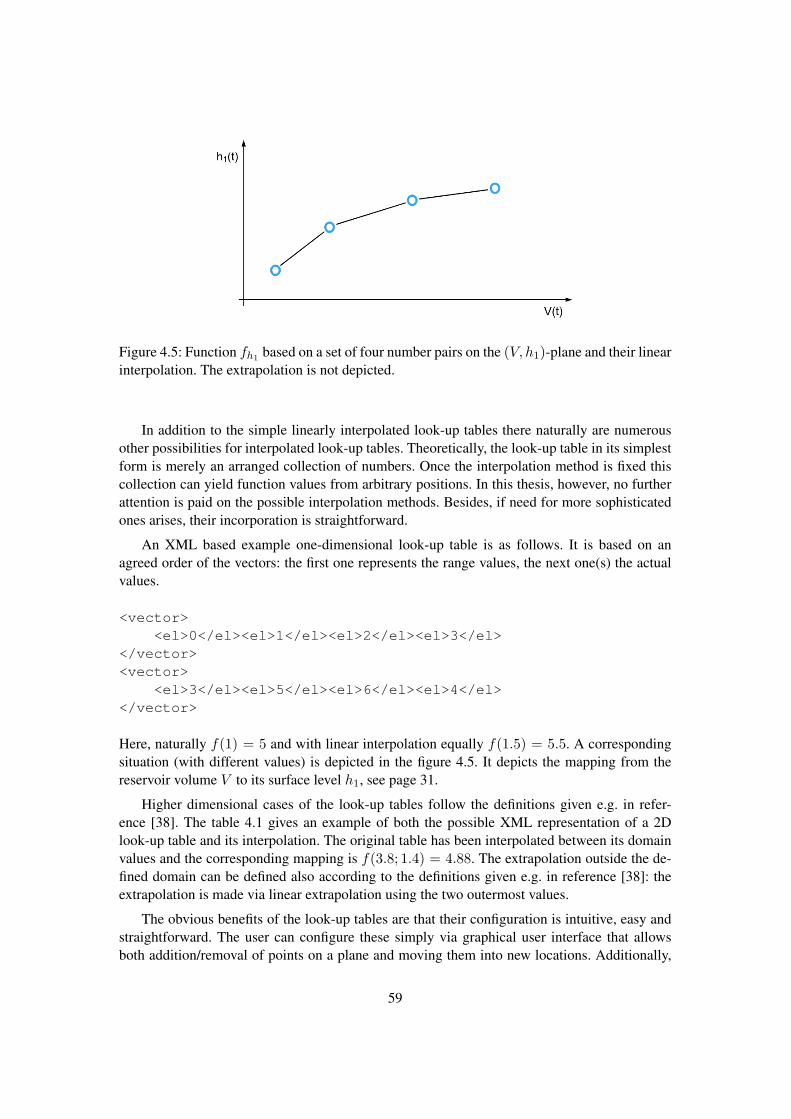
Figure 4.5: Function fh1 based on a set of four number pairs on the (V, h1)-plane and their linearinterpolation. The extrapolation is not depicted.

In addition to the simple linearly interpolated look-up tables there naturally are numerousother possibilities for interpolated look-up tables. Theoretically, the look-up table in its simplestform is merely an arranged collection of numbers. Once the interpolation method is fixed thiscollection can yield function values from arbitrary positions. In this thesis, however, no furtherattention is paid on the possible interpolation methods. Besides, if need for more sophisticatedones arises, their incorporation is straightforward.

An XML based example one-dimensional look-up table is as follows. It is based on anagreed order of the vectors: the first one represents the range values, the next one(s) the actualvalues.

<vector><el>0</el><el>1</el><el>2</el><el>3</el>

</vector><vector>

<el>3</el><el>5</el><el>6</el><el>4</el></vector>

Here, naturally f(1) = 5 and with linear interpolation equally f(1.5) = 5.5. A correspondingsituation (with different values) is depicted in the figure 4.5. It depicts the mapping from thereservoir volume V to its surface level h1, see page 31.

Higher dimensional cases of the look-up tables follow the definitions given e.g. in refer-ence [38]. The table 4.1 gives an example of both the possible XML representation of a 2Dlook-up table and its interpolation. The original table has been interpolated between its domainvalues and the corresponding mapping is f(3.8; 1.4) = 4.88. The extrapolation outside the de-fined domain can be defined also according to the definitions given e.g. in reference [38]: theextrapolation is made via linear extrapolation using the two outermost values.

The obvious benefits of the look-up tables are that their configuration is intuitive, easy andstraightforward. The user can configure these simply via graphical user interface that allowsboth addition/removal of points on a plane and moving them into new locations. Additionally,

59

<vector><el>1</el><el>3</el><el>4</el>

</vector><vector>

<el>1</el><el>2</el><el>3</el></vector><vector>

<el>3</el><el>5</el><el>6</el><el>4</el><el>3</el><el>5</el><el>6</el><el>4</el><el>4</el>

</vector>

1 2 31 3 5 63 4 3 54 6 4 4

1 1.4 2 31 3 3.8 5 63 4 3.6 3 5

3.8 5.6 4.88 3.8 4.24 6 5.2 4 4

Table 4.1: An example of a functional mapping via two-dimensional look-up table. The leftcolumn corresponds to an XML representation of the table and the right column gives both theoriginal table and a case where it has been interpolated between its domain values.

numerical configuration with corresponding graphical representation updating in real time isanother option.

4.3.2 Constraints and soft limits

There are two common types of constraints in the mathematical model:

1. upper and lower limits for both common variables and their derivatives

2. soft limits with both constraint and penalty function

They are encountered in the model so often that it is reasonable to take them as entities ontheir own rights. The first shall be called the limit constraint and the second one the soft limitconstraint. Both are discussed in the following.

The limit constraints compose of two time series: the upper and the lower limits. More ex-actly using the relations discussed earlier, there are is-part-of type relations between the limitconstraints and the time series. Hence, the possible schema formulation using the modular rep-resentation in its simplest form could be like

limit.constraint1[time.series2[#]

]

or more accurately

limit.constraint1[upper.limit.time.series1[TS]lower.limit.time.series1[TS]

]

60

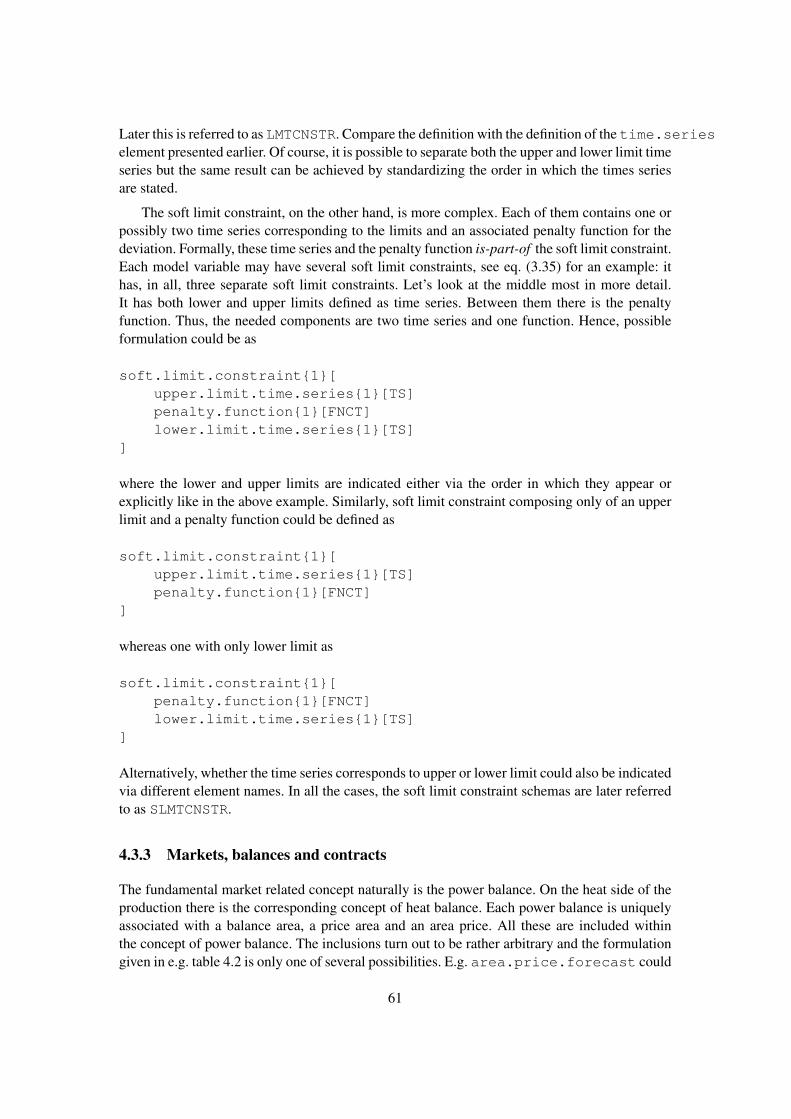
Later this is referred to as LMTCNSTR. Compare the definition with the definition of the time.serieselement presented earlier. Of course, it is possible to separate both the upper and lower limit timeseries but the same result can be achieved by standardizing the order in which the times seriesare stated.

The soft limit constraint, on the other hand, is more complex. Each of them contains one orpossibly two time series corresponding to the limits and an associated penalty function for thedeviation. Formally, these time series and the penalty function is-part-of the soft limit constraint.Each model variable may have several soft limit constraints, see eq. (3.35) for an example: ithas, in all, three separate soft limit constraints. Let’s look at the middle most in more detail.It has both lower and upper limits defined as time series. Between them there is the penaltyfunction. Thus, the needed components are two time series and one function. Hence, possibleformulation could be as

soft.limit.constraint1[upper.limit.time.series1[TS]penalty.function1[FNCT]lower.limit.time.series1[TS]

]

where the lower and upper limits are indicated either via the order in which they appear orexplicitly like in the above example. Similarly, soft limit constraint composing only of an upperlimit and a penalty function could be defined as

soft.limit.constraint1[upper.limit.time.series1[TS]penalty.function1[FNCT]

]

whereas one with only lower limit as

soft.limit.constraint1[penalty.function1[FNCT]lower.limit.time.series1[TS]

]

Alternatively, whether the time series corresponds to upper or lower limit could also be indicatedvia different element names. In all the cases, the soft limit constraint schemas are later referredto as SLMTCNSTR.

4.3.3 Markets, balances and contracts

The fundamental market related concept naturally is the power balance. On the heat side of theproduction there is the corresponding concept of heat balance. Each power balance is uniquelyassociated with a balance area, a price area and an area price. All these are included withinthe concept of power balance. The inclusions turn out to be rather arbitrary and the formulationgiven in e.g. table 4.2 is only one of several possibilities. E.g. area.price.forecast could

61

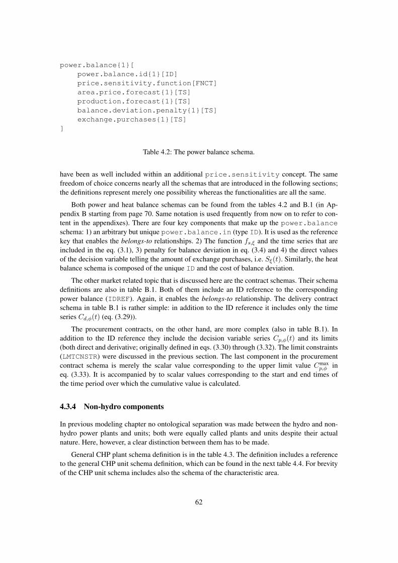
power.balance1[power.balance.id1[ID]price.sensitivity.function[FNCT]area.price.forecast1[TS]production.forecast1[TS]balance.deviation.penalty1[TS]exchange.purchases1[TS]

]

Table 4.2: The power balance schema.

have been as well included within an additional price.sensitivity concept. The samefreedom of choice concerns nearly all the schemas that are introduced in the following sections;the definitions represent merely one possibility whereas the functionalities are all the same.

Both power and heat balance schemas can be found from the tables 4.2 and B.1 (in Ap-pendix B starting from page 70. Same notation is used frequently from now on to refer to con-tent in the appendixes). There are four key components that make up the power.balanceschema: 1) an arbitrary but unique power.balance.in (type ID). It is used as the referencekey that enables the belongs-to relationships. 2) The function fs,ξ and the time series that areincluded in the eq. (3.1), 3) penalty for balance deviation in eq. (3.4) and 4) the direct valuesof the decision variable telling the amount of exchange purchases, i.e. Sξ(t). Similarly, the heatbalance schema is composed of the unique ID and the cost of balance deviation.

The other market related topic that is discussed here are the contract schemas. Their schemadefinitions are also in table B.1. Both of them include an ID reference to the correspondingpower balance (IDREF). Again, it enables the belongs-to relationship. The delivery contractschema in table B.1 is rather simple: in addition to the ID reference it includes only the timeseries Cd,φ(t) (eq. (3.29)).

The procurement contracts, on the other hand, are more complex (also in table B.1). Inaddition to the ID reference they include the decision variable series Cp,φ(t) and its limits(both direct and derivative; originally defined in eqs. (3.30) through (3.32). The limit constraints(LMTCNSTR) were discussed in the previous section. The last component in the procurementcontract schema is merely the scalar value corresponding to the upper limit value Cmax

p,φ ineq. (3.33). It is accompanied by to scalar values corresponding to the start and end times ofthe time period over which the cumulative value is calculated.

4.3.4 Non-hydro components

In previous modeling chapter no ontological separation was made between the hydro and non-hydro power plants and units; both were equally called plants and units despite their actualnature. Here, however, a clear distinction between them has to be made.

General CHP plant schema definition is in the table 4.3. The definition includes a referenceto the general CHP unit schema definition, which can be found in the next table 4.4. For brevityof the CHP unit schema includes also the schema of the characteristic area.

62

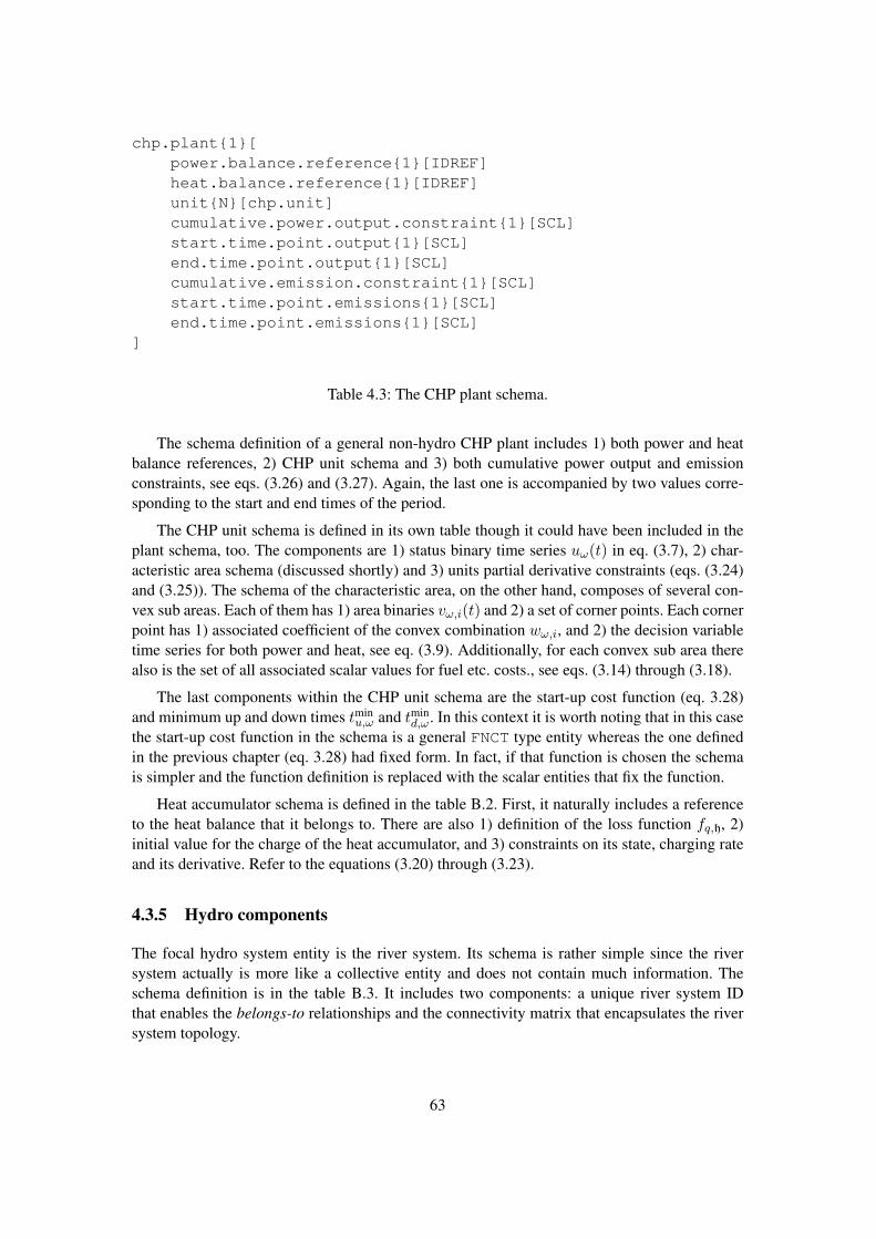
chp.plant1[power.balance.reference1[IDREF]heat.balance.reference1[IDREF]unitN[chp.unit]cumulative.power.output.constraint1[SCL]start.time.point.output1[SCL]end.time.point.output1[SCL]cumulative.emission.constraint1[SCL]start.time.point.emissions1[SCL]end.time.point.emissions1[SCL]

]

Table 4.3: The CHP plant schema.

The schema definition of a general non-hydro CHP plant includes 1) both power and heatbalance references, 2) CHP unit schema and 3) both cumulative power output and emissionconstraints, see eqs. (3.26) and (3.27). Again, the last one is accompanied by two values corre-sponding to the start and end times of the period.

The CHP unit schema is defined in its own table though it could have been included in theplant schema, too. The components are 1) status binary time series uω(t) in eq. (3.7), 2) char-acteristic area schema (discussed shortly) and 3) units partial derivative constraints (eqs. (3.24)and (3.25)). The schema of the characteristic area, on the other hand, composes of several con-vex sub areas. Each of them has 1) area binaries vω,i(t) and 2) a set of corner points. Each cornerpoint has 1) associated coefficient of the convex combination wω,i, and 2) the decision variabletime series for both power and heat, see eq. (3.9). Additionally, for each convex sub area therealso is the set of all associated scalar values for fuel etc. costs., see eqs. (3.14) through (3.18).

The last components within the CHP unit schema are the start-up cost function (eq. 3.28)and minimum up and down times tmin

u,ω and tmind,ω . In this context it is worth noting that in this case

the start-up cost function in the schema is a general FNCT type entity whereas the one definedin the previous chapter (eq. 3.28) had fixed form. In fact, if that function is chosen the schemais simpler and the function definition is replaced with the scalar entities that fix the function.

Heat accumulator schema is defined in the table B.2. First, it naturally includes a referenceto the heat balance that it belongs to. There are also 1) definition of the loss function fq,h, 2)initial value for the charge of the heat accumulator, and 3) constraints on its state, charging rateand its derivative. Refer to the equations (3.20) through (3.23).

4.3.5 Hydro components

The focal hydro system entity is the river system. Its schema is rather simple since the riversystem actually is more like a collective entity and does not contain much information. Theschema definition is in the table B.3. It includes two components: a unique river system IDthat enables the belongs-to relationships and the connectivity matrix that encapsulates the riversystem topology.

63

chp.unit1[status.binary1[TS]characteristic.area1[

convex.subareaN[area.binary1[TS]corner.pointN[

convex.coefficient1[TS]corner.point.P1[TS]corner.point.Q1[TS]

]fuel.consumption.r.01[SCL]fuel.consumption.r.P1[SCL]fuel.consumption.r.Q1[SCL]fuel.cost.c.01[SCL]fuel.cost.c.r1[SCL]emission.e.01[SCL]emission.e.r1[SCL]

]]power.output.derivative.costraint1[LMTCNSTR]heat.output.derivative.costraint1[LMTCNSTR]startup.cost.function1[FNCT]min.uptime1[SCL]min.downtime1[SCL]

]

Table 4.4: The CHP unit schema including also the schema for the characteristic area.

In hydropower context the types of the relationships again choices have to be made concern-ing the structure of the schemas. The structure of the mathematical model makes it possible tocreate one large hydro-component entity that would include all the objects excluding the riversystem itself. However, a more modular and especially a more intuitive structure is created hereusing the IDs and ID references more widely. In practice, there are IDs e.g. on the reservoirsand channels, spillways and hydro plants are related to them via ID references.

One of the most complex schema definitions in this thesis is that of reservoir’s. It can befound from the table B.4. Correspondingly, schema definitions for the channels and spillwaysare in tables B.5 and B.6. In addition to the river system and power balance ID references thereservoir schema includes definitions of functions, initial values, local time series and necessaryhard and soft constraints that can be found in section 3.7.1. Since their structure is rather simpleand analogous to the definitions discussed earlier there is no need to repeat this discussionhere. Equally, channel, spillway and hydro plant and unit schema definitions are in tables B.5through B.8.

64

Chapter 5

Discussion

Both the mathematical model and the conceptual schema covering that model have been createdin this thesis. The mathematical model was formulated based both on the academic literatureand author’s own choices. Its aim was to serve two purposes: first, to lay down detailed basisfor a simulation model to be used both for optimization result verification and simultaneouslyto set a minimum information level that has to be included into the information modeling. Thesecond objective, extensive information modeling of the algorithm-independent prerequisite in-formation, aimed at a structured and standardized representation that would enable a commonaccess to this information for all the applications that need it.

The mathematical model of the procurement planning problem has been formulated on asgeneral yet detailed level as possible. The created model is able to cover most of the basic en-ergy procurement possibilities from nuclear production to power exchange purchases. Althoughthe model is rather extensive it cannot cover all the possible details on the field. However, onthe current detail level it covers the basic information needs of any applicable optimization al-gorithm and thus reveals the arc types of the possible components. Based on the identified andmodeled components also the possible later additions can be easily structured and incorporatedinto the model.

The mathematical model combined practices from several literature sources. The most gen-eral and applicable to the BR’s procurement planning problem were chosen. In addition, in caseswhere no appropriate models could be found or where either their scope or structure was notsatisfactory the model was created based in author’s own choices. Special care was taken in thehydropower system model formulation. It was beforehand considered one of the most importantparts in this thesis. The resulting model captures the essential aspects of hydropower systemscovering a wide range from the river system level all the way to the pumps used to pump wa-ter upstream during periods of especially low electricity price. The hydropower model is bothhighly dynamical and complex; its non-linear and non-convex properties are likely to make anydirect optimization approaches effectively impossible.

The validation of the mathematical model — especially that of the hydropower sub-system— has not been done in this thesis. However, most of the chosen component models have beenused in the literature and hence considered widely accepted. Besides, the modeling accuracyhas not been considered crucial when the models are to be optimized; currently the lack ofcomputational resources limits the modeling scope considerably more.

65

The straightforwardness of the information modeling results mainly from the simplicity ofthe basic components and the fact that once the starting point is already an abstract mathematicalmodel the distinct concepts are rather readily visible. The mathematical structure itself by itsnature incorporates a great deal of the steps on the way towards conceptual schemas of thecomponents.

In this thesis the conceptual schema on the chosen domain and scope has been carefullyformulated to ensure that its transformation into extensive information model and eventuallyinto an interface file will be straightforward. The starting point for the interface design in thisthesis was the separation of the general level procurement planning system and the mathematicaloptimization algorithms. No specific algorithm had been fixed and hence the thesis has beenmade bearing in mind that the resulting interface is to transmit all the relevant informationregardless of the chosen/supported optimization algorithms. This led to significant increase inthe level of generality of the information modeling; the mere purpose of the interface is totransmit parametric information of the mathematical model whereas the mathematical structureof the model has to be assumed to be common knowledge — both the over-level procurementsupport system and the optimization applications operate on the same model whereas it is solelyup to the optimization application to decide the necessary approximations and relaxations.

The information modeling in this thesis began with definitions of concepts like ontology,entities, conceptual schemas and information models. The terminology encountered in the liter-ature is far from unique and the definitions chosen here are intuitively appealing but may fail tomatch those in other sources.

The information modeling of the BR’s procurement planning problem was eventually cul-minated into formulating structured ontology on the model objects and their parametric entities.The basis of the ontology arose naturally from the mathematical model and only some minorchanges were introduced — ontological separation between hydro and non-hydro plants doesnot exist in the mathematical model. Similarly, the mathematical model worked as a rather readybasis for modeling the relationships between entities. Only two types of relationships were in-troduced. Both the ontology and relationships are clearly present in the conceptual schemas ofthe model components, see section 4.3 and especially tables 4.2 through B.1.

In case of changes in the underlying mathematical model the reusability of the entire con-ceptual schemas themselves is not directly possible. Instead, the most basic entities and relation-ships are likely to be able to serve their purpose as the building blocks for further complicatedentities. Also, the ideas and the workflow are widely applicable and possible — or even likely —future changes can be easily implemented using the definitions of the most basic model entities.Consider an additional steam balance to be added to the mathematical model: the balance wouldcompose of the very same entities that are found within the current model. With proper ontologythis addition can be quite readily be formulated as an additional conceptual schema and addedto the interface.

Based on the work done in this thesis there are a couple of possible new research direc-tions. First, development of more algorithm-specific information models and interfaces wouldsubstantially reduce the workload of the optimization applications. Such interface could make afull use of the basic entities and their XML representations and offer a custom made access tothe very specific information with readily made approximations and relaxations. However, theproblem on this is that the interfaces become so algorithm and model specific that their usage asplatform for common access to the information is greatly reduced or completely abandoned.

66

Another possible direction for further study naturally would be a further development ofthe mathematical model. Replacing e.g. the simplifications stated above with more accurate andrealistic alternatives could increase the validity range of the model. Whether or not this is worththe work and time investments — the model is quite complex even at its present version —depend on the simultaneous development of the actual optimization engines. More likely, thecurrently necessary approximations and relations reduce the amount of details and dynamics ofthe model so significantly that more subtle nuances in the model may turn out to be completelyunnecessary.

The full applicability of the work done in this thesis can be thoroughly evaluated only witha proper implementation and empirical evidence of its usefulness and applicability in practice.The information modeling as such is a necessary step in the creation of an interface betweenapplications but whether or not it is necessary in the scope and detail it is done here is question-able until further evidence of its practicality arises. On the other hand, the mathematical modelcreated here fully serves its purpose. Even in case it contains choices that restrict its applicabil-ity or due to any other reason limit its validity or require changes, it offers a valuable source ofdetail and reference for any further work.

67

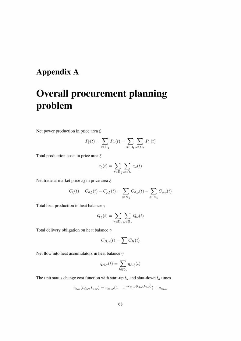
Appendix A

Overall procurement planningproblem

Net power production in price area ξ

Pξ(t) =∑π∈Πξ

Pπ(t) =∑π∈Πξ

∑ω∈Ωπ

Pω(t)

Total production costs in price area ξ

cξ(t) =∑π∈Πξ

∑ω∈Ωπ

cω(t)

Net trade at market price sξ in price area ξ

Cξ(t) = Cd,ξ(t)− Cp,ξ(t) =∑φ∈Φξ

Cd,φ(t)−∑φ∈Φξ

Cp,φ(t)

Total heat production in heat balance γ

Qγ(t) =∑π∈Πγ

∑ω∈Ωγ

Qω(t)

Total delivery obligation on heat balance γ

CH,γ(t) =∑

CH(t)

Net flow into heat accumulators in heat balance γ

qA,γ(t) =∑h∈Hγ

qA,h(t)

The unit status change cost function with start-up tu and shut-down td times

cs,ω(td,ω, tu,ω) = cs1,ω(1− e−cs2,ω(td,ω ,tu,ω)) + cs3,ω

68

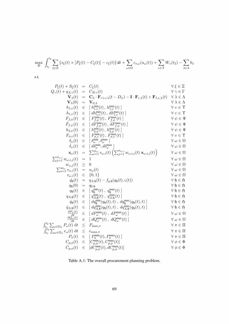
maxD

∫ t2

t1

∑ξ∈Ξ

sξ(t)× [Pξ(t)− Cξ(t)]− cξ(t) dt+∑ω∈Ω

cs,ω(uω(t)) +∑υ∈Υ

Wυ(t2)−∑λ∈Λ

bλ

s.t.

Pξ(t) + Sξ(t) = Cξ(t) ∀ ξ ∈ ΞQγ(t) + qA,γ(t) = CH,γ(t) ∀ γ ∈ Γ

Vλ(t) = Cλ · Fr+c,λ(t−Dψ)− I · Fr,λ(t) + FI,e,λ(t) ∀ λ ∈ ΛVλ(0) = V0,λ ∀ λ ∈ Λh1,υ(t) ∈ [ hmin

1,υ (t) , hmax1,υ (t) ] ∀ υ ∈ Υ

h1,υ(t) ∈ [ dhmin1,υ (t) , dhmax

1,υ (t) ] ∀ υ ∈ ΥFf,ψ(t) ∈ [ Fmin

f,ψ (t) , Fmaxf,ψ (t) ] ∀ ψ ∈ Ψ

Ff,ψ(t) ∈ [ dFminf,ψ (t) , dFmax

f,ψ (t) ] ∀ ψ ∈ Ψh2,ψ(t) ∈ [ hmin

2,ψ(t) , hmax2,ψ (t) ] ∀ ψ ∈ Ψ

Fσ,υ(t) ∈ [ Fminσ,υ (t) , Fmax

σ,υ (t) ] ∀ υ ∈ Υδω(t) ∈ [ δmin

ω , δmaxω ] ∀ ω ∈ Ω

δω(t) ∈ [ dδminω , dδmax

ω ] ∀ ω ∈ Ωxω(t) =

∑mωi=1 vω,i(t)

(∑nω,i

j=1 wω,i,j(t) xω,i,j(t))

∀ ω ∈ Ω∑nω,i

j=1 wω,i,j(t) = 1 ∀ ω ∈ Ωwω,j(t) ≥ 0 ∀ ω ∈ Ω∑mω

i=1 vω,i(t) = uω(t) ∀ ω ∈ Ωvω,i(t) ∈ 0, 1 ∀ ω ∈ Ωqh(t) = qA,h(t)− fq,h(qh(t), ς(t)) ∀ h ∈ H

qh(0) = q0,h ∀ h ∈ H

qh(t) ∈ [ qminh (t) , qmax

h (t) ] ∀ h ∈ H

qA,h(t) ∈ [ qminA,h(t) , q

maxA,h (t) ] ∀ h ∈ H

qh(t) ∈ [ dqminh (qh(t), t) , dqmax

h (qh(t), t) ] ∀ h ∈ H

qA,h(t) ∈ [ dqminA,h(qh(t), t) , dq

maxA,h (qh(t), t) ] ∀ h ∈ H

∂Pω(t)∂t ∈ [ dPmin

ω (t) , dPmaxω (t) ] ∀ ω ∈ Ω

∂Qω(t)∂t ∈ [ dQmin

ω (t) , dQmaxω (t) ] ∀ ω ∈ Ω∫ t2

t1

∑ω∈Ωπ

Pω(t) dt ≤ Pmax,π ∀ π ∈ Π∫ t2t1

∑ω∈Ωπ

eω(t) dt ≤ emax,π ∀ π ∈ ΠPπ(t) ∈ [ Pmin

π (t), Pmaxπ (t) ] ∀ π ∈ Π

Cp,φ(t) ∈ [Cminp,φ (t), Cmax

p,φ (t)] ∀ φ ∈ ΦCp,φ(t) ∈ [dCmin

p,φ (t), dCmaxp,φ (t)] ∀ φ ∈ Φ

Table A.1: The overall procurement planning problem.

69

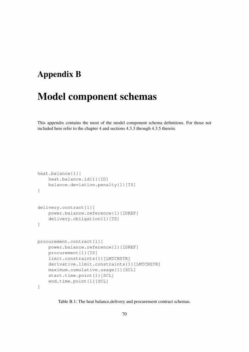
Appendix B

Model component schemas

This appendix contains the most of the model component schema definitions. For those notincluded here refer to the chapter 4 and sections 4.3.3 through 4.3.5 therein.

heat.balance1[heat.balance.id1[ID]balance.deviation.penalty1[TS]

]

delivery.contract1[power.balance.reference1[IDREF]delivery.obligation1[TS]

]

procurement.contract1[power.balance.reference1[IDREF]procurement1[TS]limit.constraints1[LMTCNSTR]derivative.limit.constraints1[LMTCNSTR]maximum.cumulative.usage1[SCL]start.time.point1[SCL]end.time.point1[SCL]

]

Table B.1: The heat balance,delivery and procurement contract schemas.

70

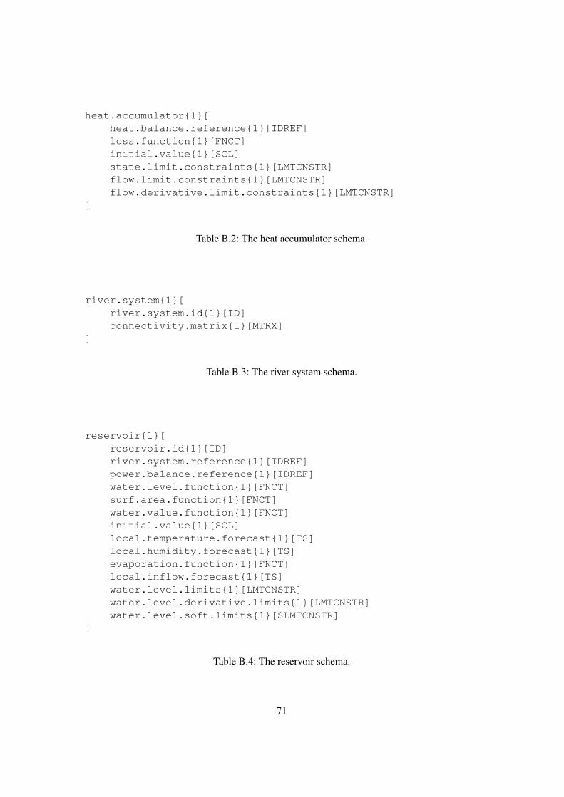
heat.accumulator1[heat.balance.reference1[IDREF]loss.function1[FNCT]initial.value1[SCL]state.limit.constraints1[LMTCNSTR]flow.limit.constraints1[LMTCNSTR]flow.derivative.limit.constraints1[LMTCNSTR]

]

Table B.2: The heat accumulator schema.

river.system1[river.system.id1[ID]connectivity.matrix1[MTRX]

]

Table B.3: The river system schema.

reservoir1[reservoir.id1[ID]river.system.reference1[IDREF]power.balance.reference1[IDREF]water.level.function1[FNCT]surf.area.function1[FNCT]water.value.function1[FNCT]initial.value1[SCL]local.temperature.forecast1[TS]local.humidity.forecast1[TS]evaporation.function1[FNCT]local.inflow.forecast1[TS]water.level.limits1[LMTCNSTR]water.level.derivative.limits1[LMTCNSTR]water.level.soft.limits1[SLMTCNSTR]

]

Table B.4: The reservoir schema.

71

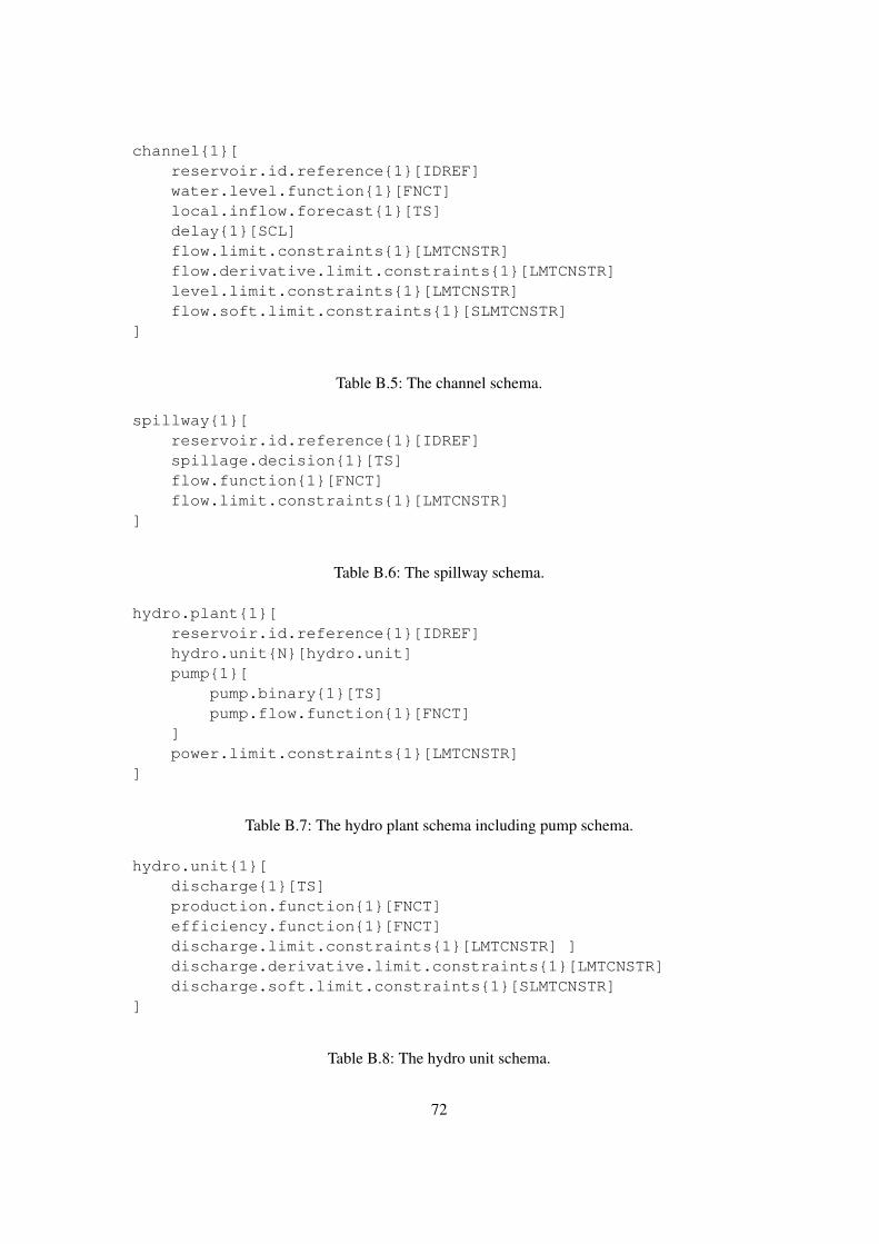
channel1[reservoir.id.reference1[IDREF]water.level.function1[FNCT]local.inflow.forecast1[TS]delay1[SCL]flow.limit.constraints1[LMTCNSTR]flow.derivative.limit.constraints1[LMTCNSTR]level.limit.constraints1[LMTCNSTR]flow.soft.limit.constraints1[SLMTCNSTR]

]

Table B.5: The channel schema.

spillway1[reservoir.id.reference1[IDREF]spillage.decision1[TS]flow.function1[FNCT]flow.limit.constraints1[LMTCNSTR]

]

Table B.6: The spillway schema.

hydro.plant1[reservoir.id.reference1[IDREF]hydro.unitN[hydro.unit]pump1[

pump.binary1[TS]pump.flow.function1[FNCT]

]power.limit.constraints1[LMTCNSTR]

]

Table B.7: The hydro plant schema including pump schema.

hydro.unit1[discharge1[TS]production.function1[FNCT]efficiency.function1[FNCT]discharge.limit.constraints1[LMTCNSTR] ]discharge.derivative.limit.constraints1[LMTCNSTR]discharge.soft.limit.constraints1[SLMTCNSTR]

]

Table B.8: The hydro unit schema.

72

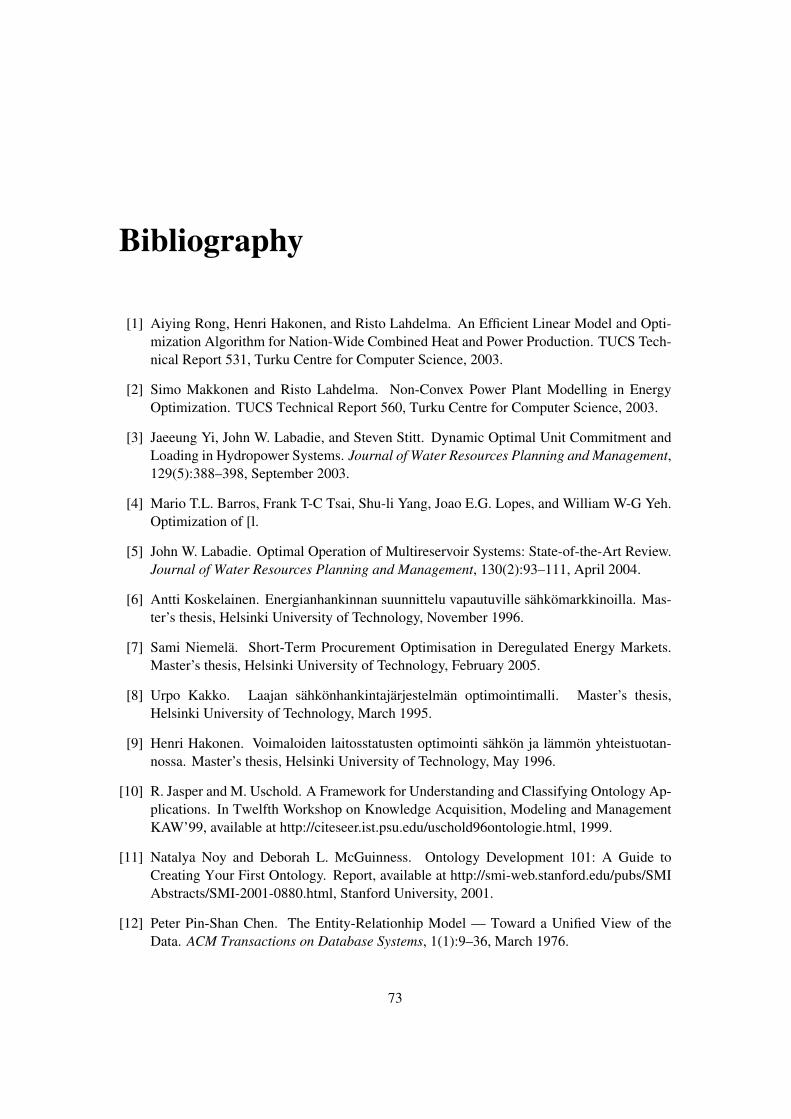
Bibliography

[1] Aiying Rong, Henri Hakonen, and Risto Lahdelma. An Efficient Linear Model and Opti-mization Algorithm for Nation-Wide Combined Heat and Power Production. TUCS Tech-nical Report 531, Turku Centre for Computer Science, 2003.

[2] Simo Makkonen and Risto Lahdelma. Non-Convex Power Plant Modelling in EnergyOptimization. TUCS Technical Report 560, Turku Centre for Computer Science, 2003.

[3] Jaeeung Yi, John W. Labadie, and Steven Stitt. Dynamic Optimal Unit Commitment andLoading in Hydropower Systems. Journal of Water Resources Planning and Management,129(5):388–398, September 2003.

[4] Mario T.L. Barros, Frank T-C Tsai, Shu-li Yang, Joao E.G. Lopes, and William W-G Yeh.Optimization of [l.

[5] John W. Labadie. Optimal Operation of Multireservoir Systems: State-of-the-Art Review.Journal of Water Resources Planning and Management, 130(2):93–111, April 2004.

[6] Antti Koskelainen. Energianhankinnan suunnittelu vapautuville sähkömarkkinoilla. Mas-ter’s thesis, Helsinki University of Technology, November 1996.

[7] Sami Niemelä. Short-Term Procurement Optimisation in Deregulated Energy Markets.Master’s thesis, Helsinki University of Technology, February 2005.

[8] Urpo Kakko. Laajan sähkönhankintajärjestelmän optimointimalli. Master’s thesis,Helsinki University of Technology, March 1995.

[9] Henri Hakonen. Voimaloiden laitosstatusten optimointi sähkön ja lämmön yhteistuotan-nossa. Master’s thesis, Helsinki University of Technology, May 1996.

[10] R. Jasper and M. Uschold. A Framework for Understanding and Classifying Ontology Ap-plications. In Twelfth Workshop on Knowledge Acquisition, Modeling and ManagementKAW’99, available at http://citeseer.ist.psu.edu/uschold96ontologie.html, 1999.

[11] Natalya Noy and Deborah L. McGuinness. Ontology Development 101: A Guide toCreating Your First Ontology. Report, available at http://smi-web.stanford.edu/pubs/SMIAbstracts/SMI-2001-0880.html, Stanford University, 2001.

[12] Peter Pin-Shan Chen. The Entity-Relationhip Model — Toward a Unified View of theData. ACM Transactions on Database Systems, 1(1):9–36, March 1976.

73

[13] Nord Pool ASA, http://www.nordpool.com/information/reports/Report-Nordic-%20Market.pdf. The Nordic Power Market, April 2004.

[14] ETSO. ETSO Scheduling System - Implementation Guide, v2r3 edition, April 2003.

[15] Jaakko Huhta. Tasevastaavan toimintoja tukeva tietojärjestelmä Suomen, Ruotsin, Taskanja Norjan kypsyneillä energiamarkkinoilla. Master’s thesis, Helsinki University of Tech-nology, March 2004.

[16] Nord Pool ASA, http://www.nordpool.com/information/reports/Report%20Spot-%20Market.pdf. Trade at Nordic Spot Market, April 2004.

[17] Henri Kokko. Energian hankinnan ja myynnin optimointi avautuneilla sähkömarkkinoilla.Master’s thesis, Helsinki University of Technology, May 2002.

[18] Eero Kukkola. Avautuneiden sähkömarkkinoiden suunnittelutehtäviä. Master’s thesis,Helsinki University of Technology, 1999.

[19] Isaac Dyner and Erik R. Larsen. From Planning to Strategy in the Electricity Industry.Energy Policy, 29:1145–1154, 2000.

[20] P. Järventausta. Tasesähkö ja säätösähkö. Tampere University of Technology, Teachingmaterial of the course Sähkömarkkinat, 2000.

[21] Donald E. Kirk. Optimal Control Theory. McMillan, 1976.

[22] H. A. Taha. Operations Research. Macmillan, New York, 1982.

[23] Arttu Lahtinen. Sopimustenhallintajärjestelmä energiakaupan päätöksenteon tukena. Mas-ter’s thesis, Helsinki University of Technology, March 2002.

[24] Pekka Pirilä. Energiatalous - Energiamarkkinat. Helsinki University of Technology, Teach-ing material of the course Energiatalous - Energiamarkkinat, 2004.

[25] S.K. Jain and D.K. Srivastava. Application of ANN for reservoir inflow prediction and op-eration. Journal of Water Resources Planning and Management, 125(5):263–271, October1999.

[26] Lennart Ljung. Modeling of Dynamic Systems. Prentice Hall, Inc., 2002.

[27] Tom R. Gruber. A Translation Approach to Portable Ontologies. Knowledge Acquisition,5(2):199–220, 1993.

[28] Pim Borst, Hans Akkermans, and Jan Top. Engineering Ontologies. International Journalof Human-Computer Studies, 46(2-3):365–406, 1997.

[29] Leena Suhl and Stephan Kassanke. Learning Object Metadata in Operations Re-search/Management Science. Learning Technology, IEEE Computer Society, 5(1), January2003.

[30] Stephan Kassanke. Ontologiebasierte Strukturierung von Lernobjekten in der DomäneOperations Research/Management Science und Einbettung in ein hypermediales Lern-system . Konzeption und Implementierung. PhD thesis, Universität Paderborn,http://www.kassanke.com/publications/, May 2004.

74

[31] Edgar F. Codd. A Relational Model of Data for Large Shared Data Banks. Communica-tions of the ACM, 13(6):377–387, 1970.

[32] M. Uschold and M. Gruninger. Ontologies: Principles, Methods and Applications. Knowl-edge Engineering Review, 11(2):93–155, 1996.

[33] David C. Fallside and Priscilla Walmsley. XML Schema. W3C — The World Wide WebConsortium, www, 2 edition, October 2004.

[34] Simon North and Paul Hermans. XML Trainer Kir. IT Press, 1 edition, 2001.

[35] Ron Ausbrooks et al. Mathematical Markup Language (MathML). W3C — The WorldWide Web Consortium, http://www.w3.org/Math/, 2 edition, October 2003.

[36] Library of Ontologies. http://sigchi.org/chi96/proceedings/papers/Rice/jpr_ht62.htm.

[37] Robert Fourer and Leo Lopes. LPFML: A W3C XML Schema for Linear Programming.Technical report, Dept. of Industrial Engineering and Management Sciences, NorthwesternUniversity, pdf@www, 2003.

[38] MathWorks. SIMULINK - Dynamic System Simulation for MATLAB, 4 edition, 2000.

75