information and volatility dynamics in the bitcoin futures...

NORTHWESTERN UNIVERSITY

Information and Volatility Dynamics in

the Bitcoin Futures Market

by

Zachary Herron

A thesis submitted in partial fulfillment for the degree of

Bachelor of Arts in Mathematical Methods in the Social Sciences

in the

Department of Mathematical Methods in the Social Sciences

April 2018

http://www.northwestern.edu/

[email protected]

”I’m talking about crypto, bro. It’s not the new

’gluten-free,’ it’s just this new thing that everyone

is doing and no one fully understands yet”

- Jimmy Tatro

NORTHWESTERN UNIVERSITY

Abstract

Department of Mathematical Methods in the Social Sciences

Bachelor of Arts in Mathematical Methods in the Social Sciences

by Zachary Herron

In this paper the interplay between the Bitcoin spot and futures markets is examined to

determine how information is flowing between the two markets. This question is inter-

esting because information flows from futures to spot markets is traditionally considered

an important requirement for futures markets to be stabilizing to spot markets. Several

statistical tests conclude that spot prices lead futures prices, and that spot volatility

may weakly lead futures volatility. This may imply information flows from the spot

market to the futures market, a surprising result that is seen in no well-established asset

class. This finding is supported by a difference-in-differences model across several cryp-

tocurrencies, finding no dampening effect on observed volatility in Bitcoin compared to

other cryptocurrencies that did not have futures contracts introduced.

http://www.northwestern.edu/

[email protected]

Contents

Abstract ii

1 Introduction 1

2 Characterization of Bitcoin Technology and Bitcoin Markets 3

2.1 Features of All Electronic Money and Digital Tokens . . . . . . . . . . . . 3

2.2 Features of Bitcoin . . . . . . . . . . . . . . . . . . . . . . . . . . . . . . . 4

2.3 Demand for Bitcoin . . . . . . . . . . . . . . . . . . . . . . . . . . . . . . 6

2.4 Spot vs. Futures Market . . . . . . . . . . . . . . . . . . . . . . . . . . . . 7

3 Literature and Theory Review 12

3.1 Theoretical Effect of Futures Markets on Spot Markets in Existing Liter-ature . . . . . . . . . . . . . . . . . . . . . . . . . . . . . . . . . . . . . . . 12

3.2 Price Lead-Lag Analysis . . . . . . . . . . . . . . . . . . . . . . . . . . . . 13

3.3 Volatility Dynamics . . . . . . . . . . . . . . . . . . . . . . . . . . . . . . 14

4 Empirical Methodology and Results 15

4.1 Data . . . . . . . . . . . . . . . . . . . . . . . . . . . . . . . . . . . . . . . 15

4.2 Price Lead-Lag Analysis . . . . . . . . . . . . . . . . . . . . . . . . . . . . 15

4.3 Volatility Dynamics . . . . . . . . . . . . . . . . . . . . . . . . . . . . . . 18

4.4 Effect of Introduction of Bitcoin Futures on Spot Volatility . . . . . . . . 22

5 Conclusion 24

A Appendix 26

Bibliography 29

iii

Chapter 1

Introduction

Many in the technology community will remember 2017 as the year of the blockchain.

The new distributed ledger technology exploded into the public psyche, and brought with

it sky-high trading prices of the money-like tokens associated with certain blockchains.

Nowhere was this trend more apparent than in Bitcoin, a token that pioneered the

cryptocurrency platform with a whitepaper authored by the pseudonymous “Satoshi

Nakamoto” in October 2008. The price of a Bitcoin surged from around $970 in Jan-

uary to over $13,000 by years end, with a corresponding “coin market capitalization” of

$220 billion1. Despite a veritable media frenzy surrounding the token and the technol-

ogy, a relative lack of economic literature exists to provide a framework for analyzing

Bitcoin. Early papers were published by technologists and lawyers, examining techno-

logical issues associated with a blockchain-based token and offering prescriptive legal

treatments for the new “money.” However, within the past 4 years, a growing corpus of

economic research has offered new ideas and approaches to explain the ascendancy of

the technology.

Of particular interest to both policy-makers and investors in Bitcoin is the unique preva-

lence of consumer investors driving the asset markets. Bitcoin skyrocketed in price with-

out any large financial institutions trading the currency. This is in stark relief to other

recent asset bubbles in assets like public equities or commercial and residential real es-

tate. The market also matured incredibly quickly, moving from a small, niche market

to over $200 billion market cap in a span of months.

In December 18, the Chicago Board of Exchange (CBOE) and Chicago Mercantile Ex-

change (CME) introduced the first financial derivatives tied to Bitcoin. Both exchanges

1coinmarketcap.com

1

Introduction 2

introduced futures contracts, with the CBOE introducing the first contract a week be-

fore the CME. This provides an interesting natural experiment. Bitcoin grew into a

massive financial market with essentially no large financial institutions moving the mar-

ket whatsoever – there were commonly days with over $15 billion in volume in late

2017. However, futures markets are driven primarily by institutional investors. Would

this influx of “smart money” smooth or exacerbate volatility? Would it help improve

price discovery, and allow for efficient mechanisms for risk transfer, liquidity, and price

visibility?

Existing theoretical models posit a number of mechanisms for this to occur. However,

numerous authors, as examined in surveys such as Hodges (1992) and Mayhew (1999),

have claimed that effects are indeterminate, and could depend heavily on underlying

assumptions or even parameter values used in models. Both surveys indicate the large

corpus of literature has oftentimes conflicting or ambiguous conclusions. These theoret-

ical models typically heavily rely on information flows from one market to another. A

well-established method for measuring the direction and effect of information flows is to

use volatility spillover analysis, in addition to price lead-lag effects.

Examining the effect of the introduction of Bitcoin futures on spot volatility may provide

another useful data point for understanding dynamics between spot and futures markets

in general, and may also provide insights narrowly into the operation of the Bitcoin

market.

A series of four statistical models are estimated to shed light on this effect. Results

of the models point towards information flows from the spot market to the futures

market, an anomaly in financial markets literature. We find that spot prices lead futures

prices and spot volatility weakly leads futures volatility. Furthermore, a difference-

in-differences model shows no evidence of Bitcoin futures introduction damping spot

volatility compared to other prominent cryptocurrencies.

Before beginning our analysis, it is critically important to understand what Bitcoin is,

and how markets for Bitcoin operate. Any inferences gleaned from the empirical analysis

are not valuable without the context of the asset in question taken into consideration.

Chapter 2

Characterization of Bitcoin

Technology and Bitcoin Markets

2.1 Features of All Electronic Money and Digital Tokens

Electronic money has been a feature of the world economy for decades. Evans (2014)

distinguishes between Card-based payment systems such as Visa and Mastercard that

move money electronically from customers to merchants, wallet providers such as PayPal

that allow users to hold a digital balance of existing currency while allowing for transac-

tions into and out of the wallet, and certain remittance providers such as Western Union

that provide a secure method to move cash electronically. For any electronic money to

have value, it is imperative that a single “token,” or unit of the electronic money, cannot

be copied and spent twice – known as the “double spending problem.”

Existing electronic money solves this issue with a centralized authority who certifies

that a party has the requisite funds to complete a transaction, typically by keeping

records of all balances and transactions in the system. There is broad consensus across

the Bitcoin literature, reflected in Dwyer (2015) and Evans (2014) that such a system

cannot function without trust in the central authority’s “competence and honesty,” and

that such trust is an ongoing requirement to allow the market to function properly.

Evans (2014) recognizes that the key innovation in digital tokens is the blockchain, a

public ledger protocol that allows for public, consensus-based authentication protocol

(performed by laborers on the network), along with a public record of all transactions.

He proposes six defining features of a “decentralized public ledger platform:” that 1) it is

internet-based, rather than existing on private networks such as those that power Visa,

3

Characterization of Bitcoin Technology and Bitcoin Markets 4

2) it includes a public ledger protocol for exchanging and recording value, existing on a

public ledger (the blockchain), 3) it includes a token or some kind of container for value,

4) an incentive scheme exists for the laborers that contribute computational processing

power necessary for the cryptographic calculations, 5) a standard open-source licensing

model is used, and 6) some sort of governance system is used for making changes to

the protocol – usually based upon a variety of consensus-based open-source governance.

Many digital tokens satisfy these distinguishing characteristics, but for the remainder

of this paper we will focus our efforts on Bitcoin, by far the most popular of the digital

tokens, and the pioneer of the technology.

2.2 Features of Bitcoin

The following are features of Bitcoin as first described in Nakamoto (2008). Bitcoin are

created in accordance with a reward system to “Miners,” the laborers that process trans-

actions to the ledger. The ledger is a database that includes every transaction, a trade

of Bitcoin from one “address” to another, and of every Bitcoin produced. This ledger

is called the blockchain. Transactions are not final until they appear in the blockchains

available from many sources – in this vein, the “correct” blockchain is the longest one

– with length defined as most combined computational difficulty. The transactions are

grouped into “blocks,” which are subsequently “chained” to previous blocks through

cryptographic techniques. This process is known as mining. Miners compete to add new

blocks to the blockchain, with each block containing a record of recent transactions and

all new Bitcoin acquired by the miner.

Each block also contains a reference to the block before it, which is the answer to a

computationally challenging mathematical problem posed in each block. The reference in

each block is unique to the problem (i.e. the problem never repeats itself exactly)1. The

process of “mining” is analogous to all computers competing to solve the cryptographic

problem, the solution to which is incredibly difficult to solve but very easy to verify once

found.

These Miners are incentivized by two reward systems for giving their computational

power to the blockchain. The first is that a miner who successfully solves the crypto-

graphic key is rewarded with newly created Bitcoin – this is the only process for creating

more Bitcoin. The amount is subject to an algorithm set forward by Nakamoto (2008):

the reward started at 50 Bitcoin per block, and is halved every 210,000 blocks – roughly

every four years. The algorithm implies a cap of roughly 21 million Bitcoin, as the

1BitcoinWiki


reward will fall to zero with block 6,930,000. With 17.0 million Bitcoin currently in

circulation2, 80% of all present and future Bitcoins have been mined. The difficulty of

the problem is automatically adjusted by an algorithm to keep the average time to solve

a block to 10 minutes3, implying 144 blocks per day, with each block restricted to 1

megabyte. These figures are all available in the source code and have been compiled by

a number of public sources, including BitcoinWiki, BitcoinBlockHalf.com, and posts on

BitcoinTalk.org by developers that manage the Bitcoin Foundation.

Since the bitcoin reward is only deposited to the bitcoin addresses specified by the miner

in the block solution, there is a good deal of idiosyncratic risk associated with this

competition. This encourages miners to “pool” their computers together, collectively

increasing their chance of a payout while splitting the payoff pro rata based on computing

power contributed. If miners are averse to idiosyncratic risk, Dwyer (2014) notes that

the resources provided for mining Bitcoin will be significantly less than the expected

value of bitcoins given as a reward for the mining. At the extreme, if all computing

power is pooled, there is no risk of losing the contest. He concludes that mining is

essential to maintain Bitcoin’s reliance on the mining system, although it has the effect

of decreasing the market competitiveness of mining.

The second way that miners are incentivized to contribute their computing power to

the blockchain is through transaction fees. These are extracted from the counterparties

in the transaction, and are typically charged on the basis of satoshis (1/100,000,000

of a Bitcoin) per byte of the transaction. The counterparties in a transaction can

choose the fee they pay, miners typically include transactions with the highest fees first,

which can lead to long waiting times for transactions with lower fees. As of October

21, 2017, the lowest fee for a zero-block wait time is 260 satoshis per byte4. With a

median transaction size of 226 bytes5, this would be equal to a fee of 58,760 satoshis

for a typical transaction. However, with the implementation of certain technological

advancements, such as SegWit-enabled wallets and the Lightning Network (the scope of

which is outside of this paper), by March 9, 2017, the corresponding fee was 20 satoshis

per byte, equivalent to 4,500 satoshis for a typical transaction.

2coinmarketcap.com3BitcoinWiki4bitcoinfees.earn.com5Ibid.


2.3 Demand for Bitcoin

Much of the debate surrounding Bitcoin centers on the demand side of the market.

Since supply is completely inelastic and determined algorithmically, price fluctuation

is by definition determined by changes in demand. Given that cryptocurrency is an

altogether new asset class, a natural question is which existing class is most appropriate

to use as a proxy for how holders of Bitcoin act. This is a question that numerous

academic papers have addressed, and is essential to the study of Bitcoin.

There is a building consensus that Bitcoin is treated by its investors as a speculative as-

set, rather than the fiat currency replacement that many claim it to be. While Dyhrberg

(2016) controversially concludes that Bitcoin acts as a gold-currency hybrid, many au-

thors and bloggers publicly disagreed with her conclusions. Notably, her conclusions

were sharply rebuked by Baur, Dimpfl, and Kuck (2017), who, in a replication study,

claim that the method cannot answer the research question posed. They contend further

that Bitcoin has unique risk-return characteristics and is virtually uncorrelated with re-

turns to other financial and nonfinancial assets considered. The group concludes that

the extremely high volatility and inflated excess returns associated with Bitcoin position

it as a speculative asset, rather than a currency or commodity.

Glaser, Zimmermann, Haferkorn, Weber, and Siering (2014) propose to answer a similar

question: what are the intentions of users who exchange “normal” currency to Bitcoin.

They too, conclude that users that purchase Bitcoin are doing so primarily as an alterna-

tive speculative financial asset, rather than to take advantage of its payment processing

network. Although this study occurred relatively early in the adoption stages of the

technology, many of its observations about the platform have stood the test of time.

Yermack (2013) supports this frame, arguing that Bitcoin is not currently currency, nor

will it be in the future.

International financial market participants may also be using Bitcoin as a disaster asset,

contends Viglione (2015) in a paper that finds a relationship between low economic

freedom of a country and higher Bitcoin premiums on exchanges in that country. This

would imply that Bitcoin functions as a catastrophe asset for hedging domestic financial

repression, functioning in an imperfect market with “unexpectedly high premiums.”


2.4 Spot vs. Futures Market

The decentralized and (functionally) anonymous nature of bitcoin ownership, combined

with exchanges that are secretive and privately held, prevents an exact tabulation of

who owns and trades Bitcoin. Traditional institutional investors, such as mutual funds,

investment banks, pension funds, and hedge funds that trade in other assets as well

as cryptocurrency, are anecdotally absent from the meteoric rise in Bitcoin price. The

reasons for this are varied.

Goldman Sachs, along with other large investment banks, actively decided not to invest

in the Cryptocurrency space due to the nascent stage of market development and unclear

regulatory environment. No large investment banks have publicly announced that they

own or run a cryptocurrency trading desk, and rumors circulated around October 2017

that Goldman was considering opening the first such operation on Wall Street6. How-

ever, Goldman’s CEO, Lloyd Blankfein, at the 2018 World Economic Forum in Davos,

stated that such rumors were false, and the bank’s only involvement with Bitcoin was

to clear futures contracts with clients in its capacity as a prime broker7.

Traditional mutual funds and ETFs in the United Kingdom were restricted from owning

Bitcoin, as it was not a traditional security regulated by the primary regulators in the

space, the Securities and Exchange Commission and the Financial Conduct Authority8.

Fintech research firm Autonomous NEXT recorded a record high of 226 global hedge

funds focused on trading crypto currency, but with aggregate assets under management

of between $3.5 and $5 billion9. This is large growth from previous years, but a proverbial

“drop in the bucket” where the global cryptocurrency market cap peaked at over $700

billion, and rests at $373 billion on March 13, 201810.

This absence of institutional money in Bitcoin spot markets is starkly contrasted by

the preponderance of institutional money in futures markets. CBOE Bitcoin futures

information is reported to the Commodity Futures Trading Commission (CFTC) in

the United States, an important regulator of futures and swaps markets. This data

captures a number of important characteristics of the Bitcoin futures market. Contract

holders are divided by type: Dealer Intermediary, Asset Manager, Leveraged Funds,

Other Reportables, and Nonreportable positions. An immediately striking observation

is the absolute lack of involvement of “Asset Managers,” or “Institutional Buyers” in the

6Wall Street Journal, “Goldman Sachs Explores a New World, Trading Bitcoin”7Wall Street Journal, “Goldman CEO Lloyd Blankfein Talks Taxes, Politics, and Trading from Davos”8Financial Times, “Big Investors Yet to Invest in Bitcoin”9Autonomous NEXT, web

10coinmarketcap.com


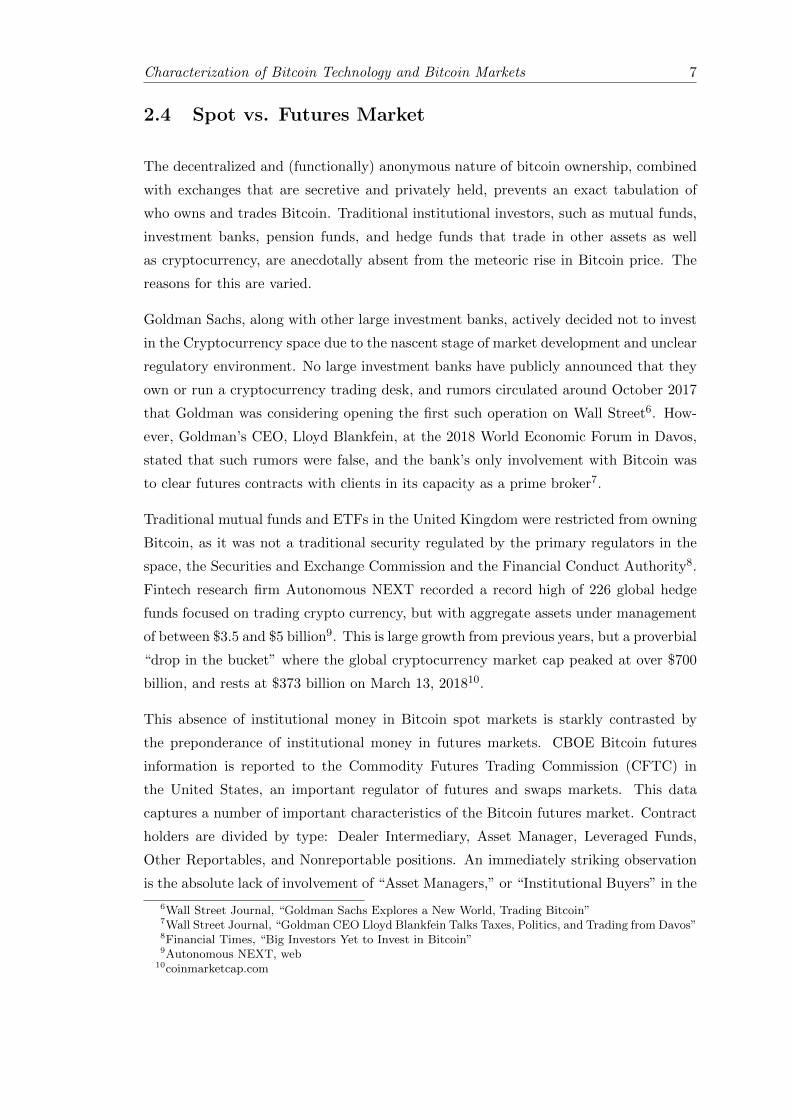
Figure 2.1: Composition of Bitcoin Futures Positions – CBOE Contracts

market, with only 1.0% of total positions outstanding11. The CFTC defines this group

as including “pension funds, endowments, insurance companies, mutual funds, and those

portfolio/investment managers whose clients are predominantly institutional”12. This

data mirrors anecdotal evidence of a lack of involvement by these parties in the spot

market, and would seem to support the conclusion that heavily-regulated or conservative

investors steer clear from cryptocurrency markets altogether.

Perhaps unsurprisingly, the majority of positions are held by traders or institutions with

“reportable” positions – defined by the CFTC as larger than 25 contracts. This includes

“Leveraged Funds,” characterized as “typically hedge funds and various types of money

managers, including registered commodity trading advisors (CTAs); registered commod-

ity pool operators (CPOs), or unregistered funds,” and “Other Reportables,” typically

other financial institutions not captured under any of the other categorizations13. This

trend would likely be amplified in the CME futures market, as the contract size is 5

Bitcoin, compared to the CBOE contract size of 1 Bitcoin14. This supports the con-

clusion that larger institutional investors are driving movements in the futures market,

rather than retail investors. Large investors certainly account for a greater percentage

11Commodity Futures Trading Commission, “Traders in Financial Futures”12Commodity Futures Trading Commission, “Traders in Financial Futures – Explanatory Notes”13Commodity Futures Trading Commission, “Traders in Financial Futures – Explanatory Notes”14CME Group


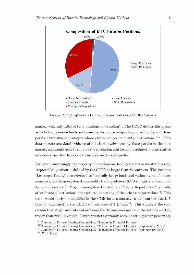
Figure 2.2: Composition of S&P500 Index Futures Positions – CBOE Contracts

of volume and outstanding positions in the futures market compared to the spot market

for Bitcoin.

Of note, however, is that nonreportable positions hold a comparably large portion of total

Bitcoin future positions compared to more traditional asset classes. As seen in ??, small,

nonreportable positions of fewer than 25 contracts (with each contract representing a

notional value of the SP500 Index mulplied by $250), nonreportable positions account

for only 11.6% of total SPX Futures positions. This is likely to reflect reluctance of

established financial firms and funds, who are typically categorized as “Asset Managers”

or “Dealer Intermediary” in the data, to hold a derivative of such a volatile and poorly

understood underlying asset, in a market that is not quite mature yet. When large

firms categorized as Dealer Intermediaries or Asset Managers are removed from the

SPX Positions, the Nonreportable positions share of the remaining positions is much

closer to its proportion of Bitcoin futures positions.

Furthermore, the Nonreportable Positions held a disproportionate level of the long posi-

tions in the futures market, with roughly 46% of all long positions in the whole market.

This is perhaps unsurprising, given the anecdotal evidence of bearish opinions from the

Wall Street establishment, and that the meteoric bull run in the spot market was driven

primarily by retail activity. This disparity may also indicate that retail investors are not

trading based upon signals from (traditionally considered) more highly sophisticated

investors. Bitcoin’s roots as a decentralized, anti-establishment product (forming an


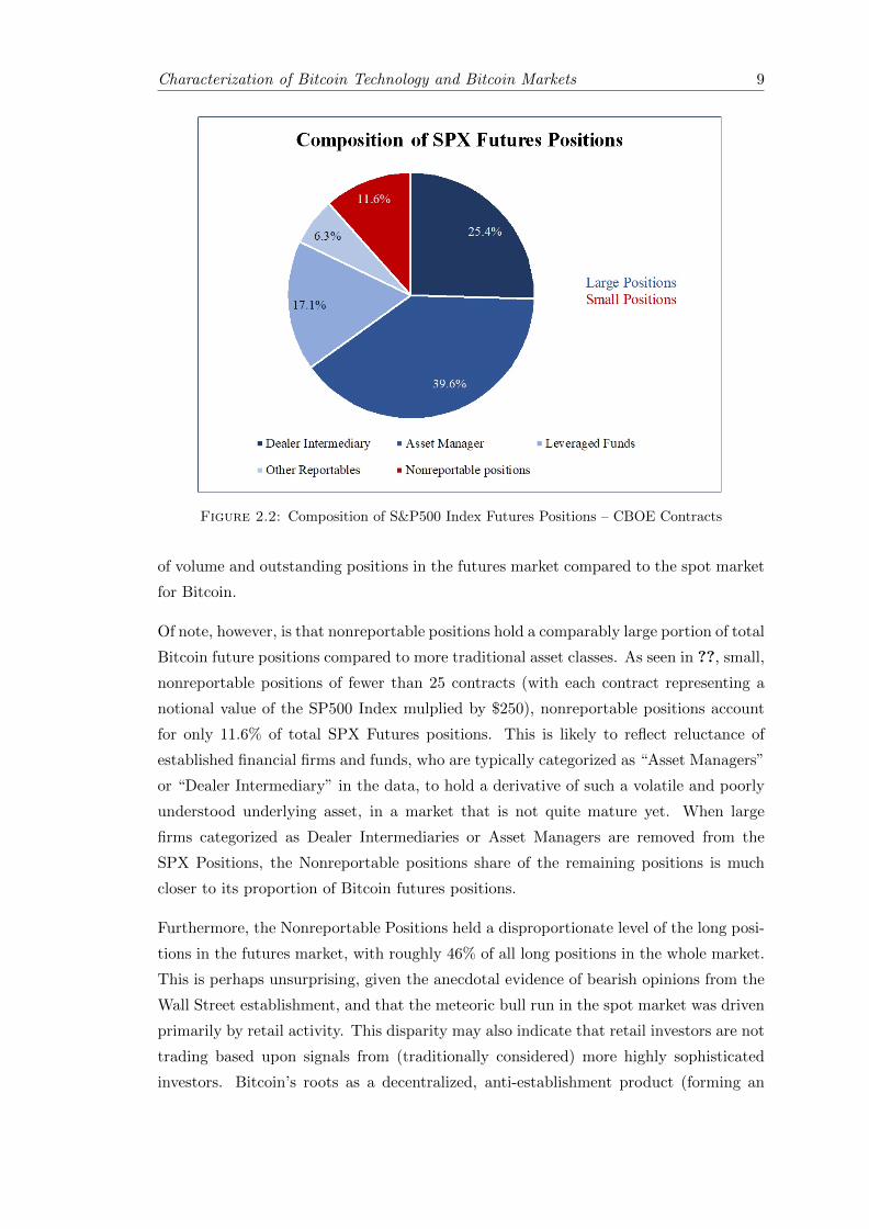
Figure 2.3: Total Bitcoin Futures Positions, Excluding Straddles – CBOE Contracts

anti-establishment community rejecting the existing financial hegemony of Wall Street)

make this observation seem plausible. This would also fit well with the assumption that

most Nonreportable Positions are retail investors (although it is of course speculation).

This trend of bullish small investors doesn’t hold in more traditional asset classes, such

as SPX Futures. In this instance, small investors are still bullish on balance, but the

split is much closer to even. Leveraged funds are also much less bearish – although

they are still on balance bearish, the divide is much smaller than in the Bitcoin futures

market, where short contract positions outnumber long contract positions by almost 3

to 1.

Of critical importance in this data is the total size of the Bitcoin futures market. With

an open interest of 5,563 on March 6, 2018, and an opening price of $11,50015, the

total notional value of these contracts was about $64 million. With an open interest

of 1,584 on the CME contracts for the same day16, , the total notional value of the

Bitcoin futures market was just over $155 million. This is just 0.1% of the $157.7

billion market capitalization of Bitcoin on that day. This compares unfavorably to more

traditional markets. As an example, on CME Consolidated SP 500 Futures, the open

15coinmarketcap.com16CME Group


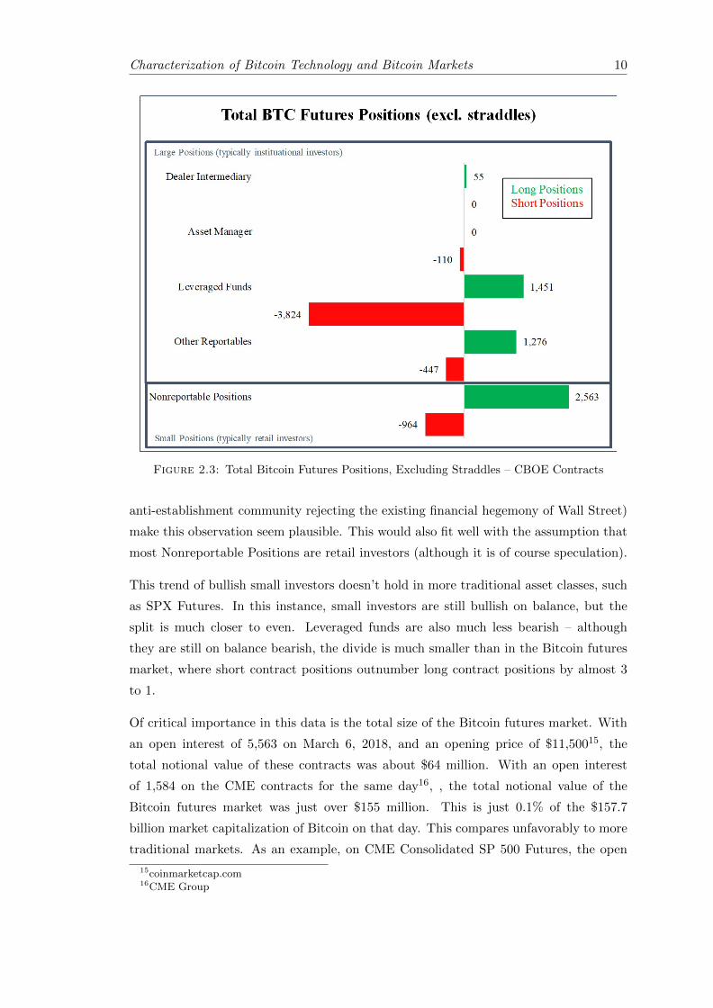
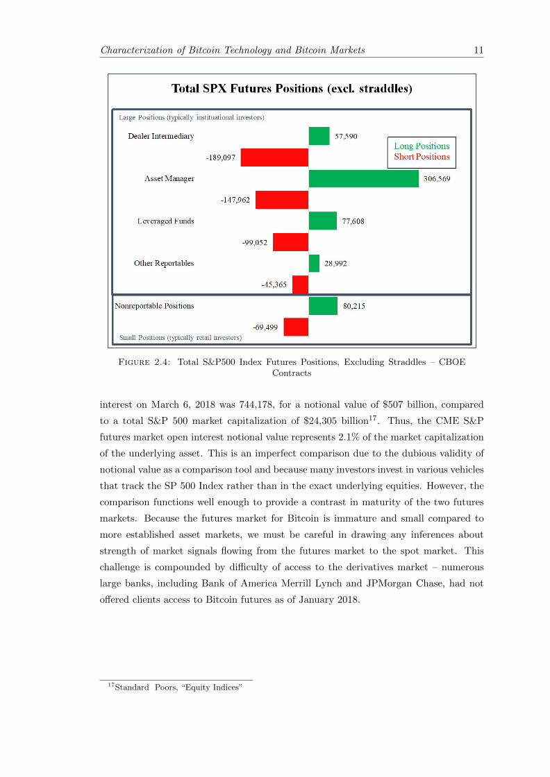
Figure 2.4: Total S&P500 Index Futures Positions, Excluding Straddles – CBOEContracts

interest on March 6, 2018 was 744,178, for a notional value of $507 billion, compared

to a total S&P 500 market capitalization of $24,305 billion17. Thus, the CME S&P

futures market open interest notional value represents 2.1% of the market capitalization

of the underlying asset. This is an imperfect comparison due to the dubious validity of

notional value as a comparison tool and because many investors invest in various vehicles

that track the SP 500 Index rather than in the exact underlying equities. However, the

comparison functions well enough to provide a contrast in maturity of the two futures

markets. Because the futures market for Bitcoin is immature and small compared to

more established asset markets, we must be careful in drawing any inferences about

strength of market signals flowing from the futures market to the spot market. This

challenge is compounded by difficulty of access to the derivatives market – numerous

large banks, including Bank of America Merrill Lynch and JPMorgan Chase, had not

offered clients access to Bitcoin futures as of January 2018.

17Standard Poors, “Equity Indices”

Chapter 3

Literature and Theory Review

3.1 Theoretical Effect of Futures Markets on Spot Markets

in Existing Literature

Numerous theoretical approaches have been proposed over the years to explain the link

between futures markets and spot markets for various assets. Given that derivatives

markets are typically speculative in nature (especially with a financial asset as the un-

derlying), much of the conversation about the role of speculative activity in financial

markets is applicable. Observations about the role of speculation go back to antiquity,

and are formalized as early as with Adam Smith (1776), who remarks that speculators

may assuage the damage done by grain shortages by purchasing and storing grain when

they forecasted a shortage. This would lead to less extreme shortages, thus leading to

less extreme price movements. John Stuart Mill (1871) added to this literature, pos-

tulating that speculators could stabilize prices by buying low and selling high, improv-

ing intertemporal efficiency of resource allocation. Milton Friedman (1953) conjectured

“Friedman’s Proposition,” the suggesting that for speculation to be profitable, it must

be price stabilizing. Since not all speculators exited markets due to bankruptcy, the ones

that remained must be assisting to stabilize prices. These classical economists spawned a

great debate about the role of speculation or speculative markets in the volatility of spot

markets, a literature that would grow exponentially with the introduction of derivatives

markets during the financially innovative period of the mid-to-late 20th century.

Much of the theoretical work surrounding futures contracts was developed for commodi-

ties that were generally storable (at some cost), and producible (at some cost). Mayhew

(1999) notes that given an intertemporal production model, intertemporal reallocation

12

Literature and Theory Review 13

may result in trading that effectively acts as an inventory management system. How-

ever, in any market that experiences random shocks, such inventory management, which

necessarily involves storage of an asset, becomes risky. Any producer or buyer that is

risk averse will thus allocate both production and purchases in an intertemporally inef-

ficient manner. Given the lack of a futures market, actors’ will only hold an asset if it

is profitable to do so, meaning that the return from holding it more than compensates

the price risk of holding it. Thus, the efficiency of intertemporal allocation is highly

dependent on the extent to which “the commodity is storable, the relative magnitude

of the predictable and random components of supply and demand changes, and the

speculators’ level of risk aversion” (Mayhew 1999). However, with the introduction of

a futures market, the carrying risk becomes zero, as a buyer or seller can immediately

lock in a price for future exchange. If agents in the model have risk aversion, then in-

tertemporal price and volatility smoothing should follow. This analysis is the classical

framework from which theoretical models involving futures markets were developed. In

Bitcoin futures markets, there is no carrying cost, meaning the commodity is essentially

perfectly storable (minus the risk of hacking). However, in such an undeveloped market,

the unexpected components of demand are large. In this framework, futures may allow

visibility into trader’s levels of anticipated demand.

Much initial work showed that the effect of a futures market should be stabilizing. Peck

(1976), Kawai (1983), Sarris (1984), and Turnovsky (1983) all developed rational ex-

pectations theoretical models with clear conclusions that futures markets are stabilizing

for nearly all plausible parameter values. However, further rational expectations models

such as those proposed by Chari and Jagannathan (1990) claim that futures markets

may be destabilizing to spot prices. Notably, all of these models incorporate information

flows from futures market activity to spot market activity.

3.2 Price Lead-Lag Analysis

There are two prevalent views on the method by which prices form in futures markets. In

one view, the intertemporal difference is accounted for by the cost of buying and storing

the commodity, as stated in Working (1948). Given that Bitcoin are easily storable

with little to no cost, it may be more accurate to think of a negative storage cost – a

convenience yield. The other view states that the intertemporal difference is due to the

composition of the spot price, a risk premium, and an expected future spot price. This

formula is expressed as

Literature and Theory Review 14

F tt − St = Et[P (t, T )] + Et[ST − St] (3.1)

With

Et[P (t, T )] = F Tt − Et[St] (3.2)

in Asche, Guttormsen (2002), where the term Et[P (t, T )] is the bias of the future price as

a forecast of the future spot price. Both views indicate a strong relationship between the

futures and spot prices, with the relationship closer for shorter maturities. Furthermore,

if the future price is to be an unbiased indicator of a subsequent spot price, (i.e. the

Et[P (t, T )] term is zero), the future price should lead the spot price. Other papers

give different arguments for futures prices to lead spot price. Silvapulle and Moosa

(1999) claim that futures are faster to incorporate new information because of the lower

transaction costs and ease of shorting. In this framework, futures prices should lead

spot prices. Others claim that futures prices may lead spot prices due to ease of market

manipulation in the futures market, or because of faster, better-informed actors in the

futures market. In this view, spot markets may be taking information cues from the

futures market. Thus, a lead-lag relationship may be informative of information flows

from the futures market to the spot market.

3.3 Volatility Dynamics

Much empirical attention was turned to the question of how futures markets could

be stabilizing or destabilizing after the advent of such predictive theoretical results.

The theory and empirical application of volatility flows using a GARCH model was

pioneered by Engle, Ito, and Lin (1990). They characterized asset volatility shocks on

a single underlying asset in many geographically distinct markets as a “meteor shower”

rather than a “heat wave” – as a meteor shower observed in New York would likely be

observed in Tokyo some hours later due to the rotation of the earth, while a heat wave

in New York would not be predictive of high temperatures in Tokyo. They found that

even country-specific shocks, such as an anticipated change in Federal Reserve policy,

would have effects on volatility in worldwide markets with some time lag. Chan, Chan,

and Karolyi (1991) noted that volatility spillover analysis can provide a useful tool for

measuring information flows.

Chapter 4

Empirical Methodology and

Results

4.1 Data

Data for Bitcoin spot and future market data are collected at the level of individual

trades. Both series are collected for all dates from December 18, 2017 to March 13, 2018.

Individual trades for Bitcoin are recorded from the Bitfinex exchange using the exchange

API. This exchange is chosen because of its dominance in the BTC-USD market; Bitfinex

has had the largest volumes of all BTC-USD exchanges for the duration of the selected

time period. Trade-level data from the futures market is retrieved from the CME Group

API. The CME exchange is chosen because of comparably larger volumes of contracts

traded compared to the CBOE.

4.2 Price Lead-Lag Analysis

This empirical analysis is conducted using an Error Correction Model as in Engle,

Granger (1987). A more robust model for establishing exogeneity, the Johansen Test

as performed in Asche, Guttormsen (2002), was rejected because of a lack of volume in

contracts of maturities longer than 2 months.

Individual trade level data is first collected into a given aggregation time period, chosen

to be 5 minutes in the results presented (although the same effect was present across

sampling periods). Prices for both close-maturity futures contracts and spot sales are

calculated by the last price in the trading period, and then logs of price are calculated.

15

Empirical Methodology and Results 16

Trading periods with no futures trading volume, such as holidays, are excluded from the

calculation. As in traditional cointegration analysis, the long-run equilibrium regression

is run first:

ft − β0 − β1st = et (4.1)

In this equation, st is the log of spot price and ft is the log of the nearest-maturity

futures price. Of note is that if β1 = 1, the markets are efficient. Furthermore, given

that the series is cointegrated, the error term in this regression should be stationary. The

stationarity of the error term is tested for using an Augmented Dickey-Fuller Test on the

residuals of the regression. The results of the regression and Augmented Dickey-Fuller

Test are given below. The ADF lag period is chosen by beginning with a large number

of lags and then removing lags that are not significant. Note that standard errors are

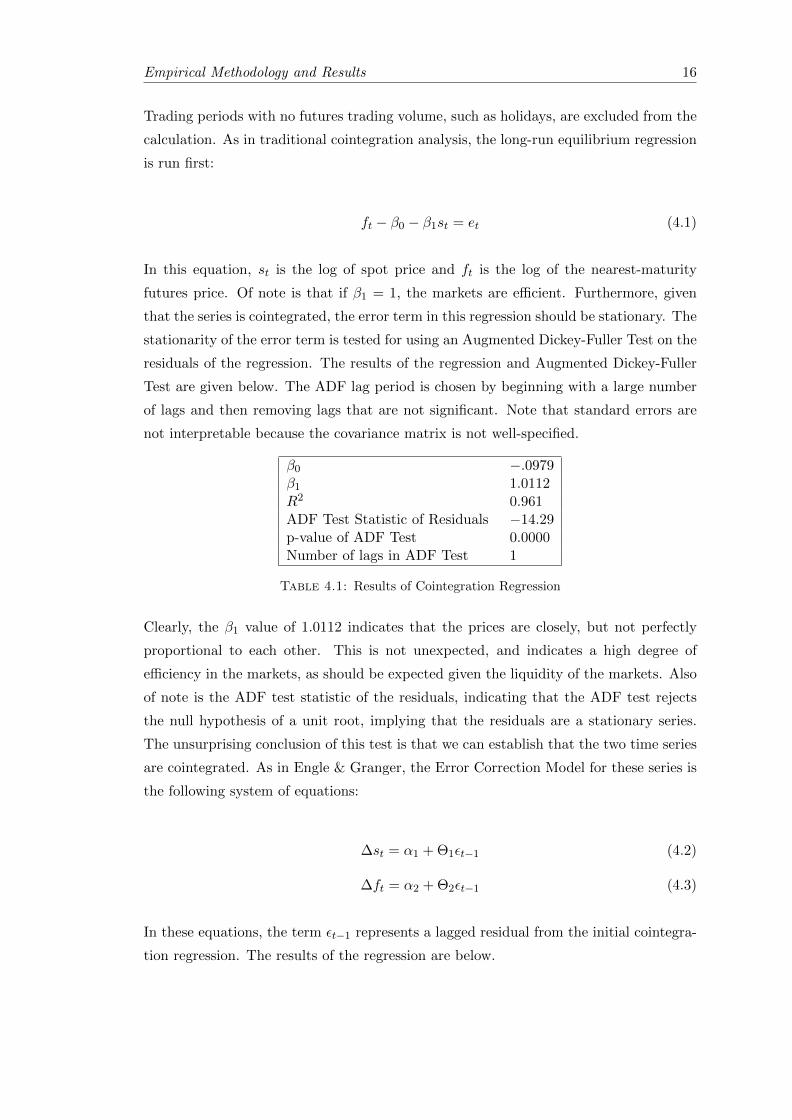
not interpretable because the covariance matrix is not well-specified.

β0 −.0979β1 1.0112R2 0.961ADF Test Statistic of Residuals −14.29p-value of ADF Test 0.0000Number of lags in ADF Test 1

Table 4.1: Results of Cointegration Regression

Clearly, the β1 value of 1.0112 indicates that the prices are closely, but not perfectly

proportional to each other. This is not unexpected, and indicates a high degree of

efficiency in the markets, as should be expected given the liquidity of the markets. Also

of note is the ADF test statistic of the residuals, indicating that the ADF test rejects

the null hypothesis of a unit root, implying that the residuals are a stationary series.

The unsurprising conclusion of this test is that we can establish that the two time series

are cointegrated. As in Engle & Granger, the Error Correction Model for these series is

the following system of equations:

∆st = α1 + Θ1εt−1 (4.2)

∆ft = α2 + Θ2εt−1 (4.3)

In these equations, the term εt−1 represents a lagged residual from the initial cointegra-

tion regression. The results of the regression are below.


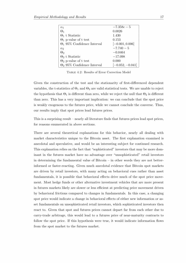
α1 −7.358e− 5Θ1 0.0026Θ1 t Statistic 1.430Θ1 p-value of t test 0.153Θ1 95% Confidence Interval [−0.001, 0.006]α2 −7.740 − 5Θ2 −0.0464Θ2 t Statistic −17.098Θ2 p-value of t test 0.000Θ2 95% Confidence Interval [−0.052,−0.041]

Table 4.2: Results of Error Correction Model

Given the construction of the test and the stationarity of first-differenced dependent

variables, the t-statistics of Θ1 and Θ2 are valid statistical tests. We are unable to reject

the hypothesis that Θ1 is different than zero, while we reject the null that Θ2 is different

than zero. This has a very important implication: we can conclude that the spot price

is weakly exogenous to the futures price, while we cannot conclude the converse. Thus,

our results imply that spot prices lead futures prices.

This is a surprising result – nearly all literature finds that futures prices lead spot prices,

for reasons enumerated in above sections.

There are several theoretical explanations for this behavior, nearly all dealing with

market characteristics unique to the Bitcoin asset. The first explanation examined is

anecdotal and speculative, and would be an interesting subject for continued research.

This explanation relies on the fact that “sophisticated” investors that may be more dom-

inant in the futures market have no advantage over “unsophisticated” retail investors

in determining the fundamental value of Bitcoin – in other words they are not better-

informed or faster-reacting. Given much anecdotal evidence that Bitcoin spot markets

are driven by retail investors, with many acting on behavioral cues rather than asset

fundamentals, it is possible that behavioral effects drive much of the spot price move-

ment. Most hedge funds or other alternative investment vehicles that are more present

in futures markets likely are slower or less efficient at predicting price movement driven

by behavioral frictions compared to changes in fundamentals. In this case, a changing

spot price would indicate a change in behavioral effects of either new information or as-

set fundamentals on unsophisticated retail investors, which sophisticated investors then

react to. Given that spot and futures prices cannot depart far from each other due to

carry-trade arbitrage, this would lead to a futures price of near-maturity contracts to

follow the spot price. If this hypothesis were true, it would indicate information flows

from the spot market to the futures market.


Another explanation could be a lack of liquidity and thickness in the futures market.

Given a change in information, a sophisticated actor in the futures market may want

to act on such information. However, such an actor may be unable to fill orders large

enough, fast enough to move the futures price faster than the spot price, where markets

are generally more well-established, liquid, and thicker. The data does indicate that

the Bitcoin futures market is smaller and less liquid compared to many other, more

traditional asset classes. However, nearly all literature finds futures prices leading spot

prices, regardless of market. In addition, no research such as this has been conducted

on a futures market with such a comparably large, retail-driven spot market. However,

if such an explanation were correct, then it would not imply information flows from the

spot market to the futures market.

4.3 Volatility Dynamics

Volatility dynamics are first measured using a GARCH framework as pioneered in Engle,

Ito, Lin (1990) and Chan, Chan, Karolyi (1991). Price data is sampled at 2 hour

intervals to reduce the white-noise effects of intraday price movements that would affect

shorter sample periods. First, prices are converted into log returns to reduce effects

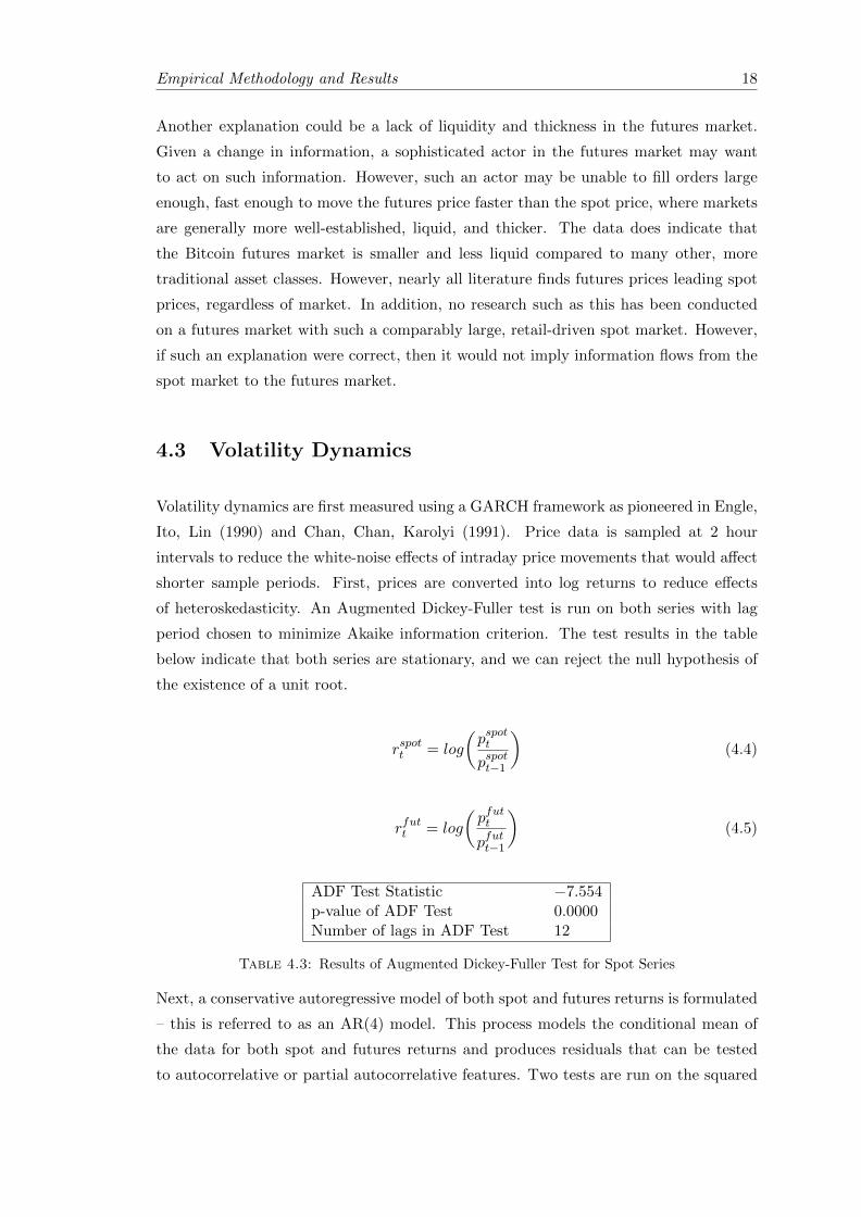
of heteroskedasticity. An Augmented Dickey-Fuller test is run on both series with lag

period chosen to minimize Akaike information criterion. The test results in the table

below indicate that both series are stationary, and we can reject the null hypothesis of

the existence of a unit root.

rspott = log

(pspott

pspott−1

)(4.4)

rfutt = log

(pfutt

pfutt−1

)(4.5)

ADF Test Statistic −7.554p-value of ADF Test 0.0000Number of lags in ADF Test 12

Table 4.3: Results of Augmented Dickey-Fuller Test for Spot Series

Next, a conservative autoregressive model of both spot and futures returns is formulated

– this is referred to as an AR(4) model. This process models the conditional mean of

the data for both spot and futures returns and produces residuals that can be tested

to autocorrelative or partial autocorrelative features. Two tests are run on the squared


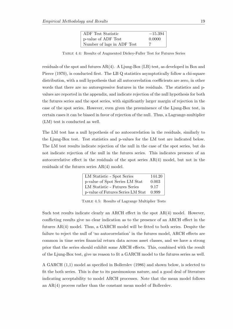
ADF Test Statistic −15.394p-value of ADF Test 0.0000Number of lags in ADF Test 7

Table 4.4: Results of Augmented Dickey-Fuller Test for Futures Series

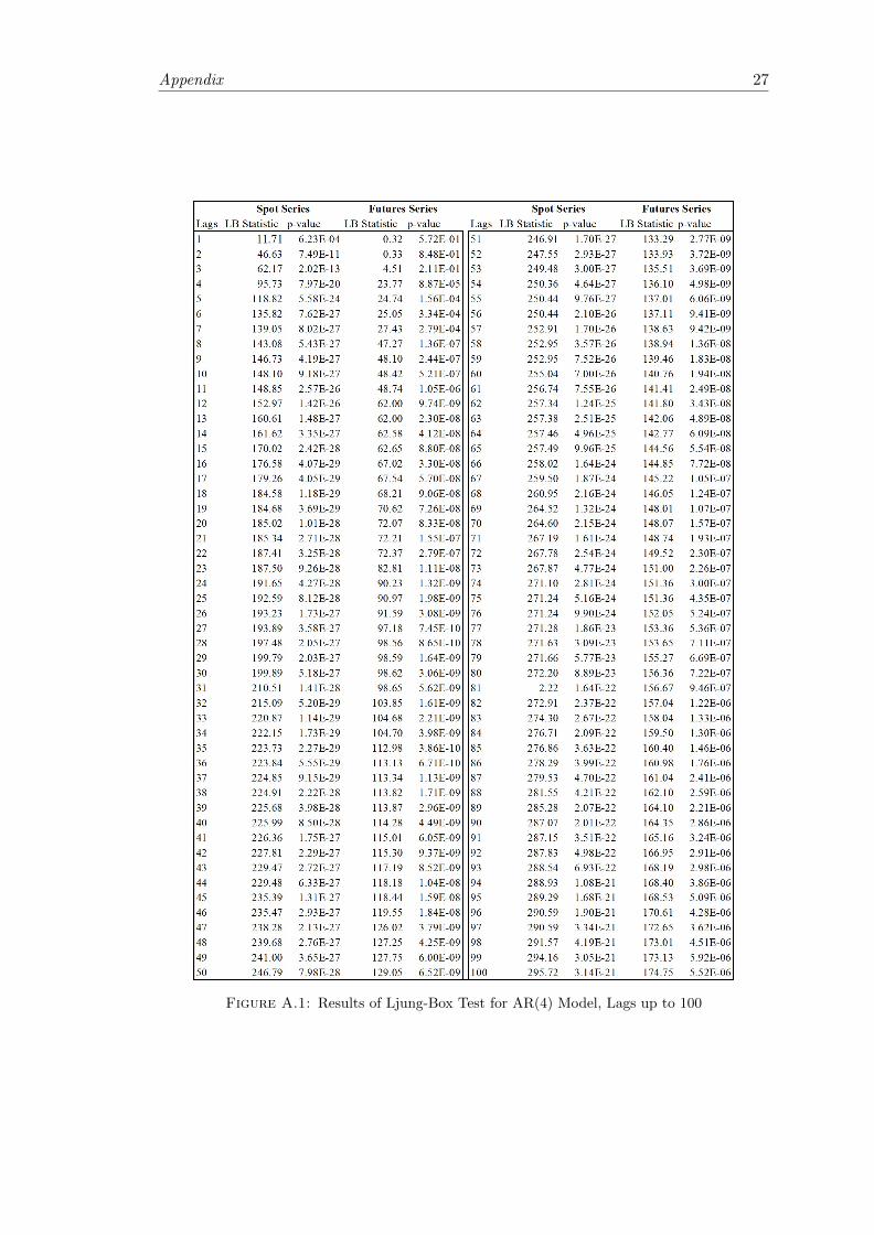
residuals of the spot and futures AR(4). A Ljung-Box (LB) test, as developed in Box and

Pierce (1970), is conducted first. The LB Q statistics asymptotically follow a chi-square

distribution, with a null hypothesis that all autocorrelation coefficients are zero, in other

words that there are no autoregressive features in the residuals. The statistics and p-

values are reported in the appendix, and indicate rejection of the null hypothesis for both

the futures series and the spot series, with significantly larger margin of rejection in the

case of the spot series. However, even given the preeminence of the Ljung-Box test, in

certain cases it can be biased in favor of rejection of the null. Thus, a Lagrange-multiplier

(LM) test is conducted as well.

The LM test has a null hypothesis of no autocorrelation in the residuals, similarly to

the Ljung-Box test. Test statistics and p-values for the LM test are indicated below.

The LM test results indicate rejection of the null in the case of the spot series, but do

not indicate rejection of the null in the futures series. This indicates presence of an

autocorrelative effect in the residuals of the spot series AR(4) model, but not in the

residuals of the futures series AR(4) model.

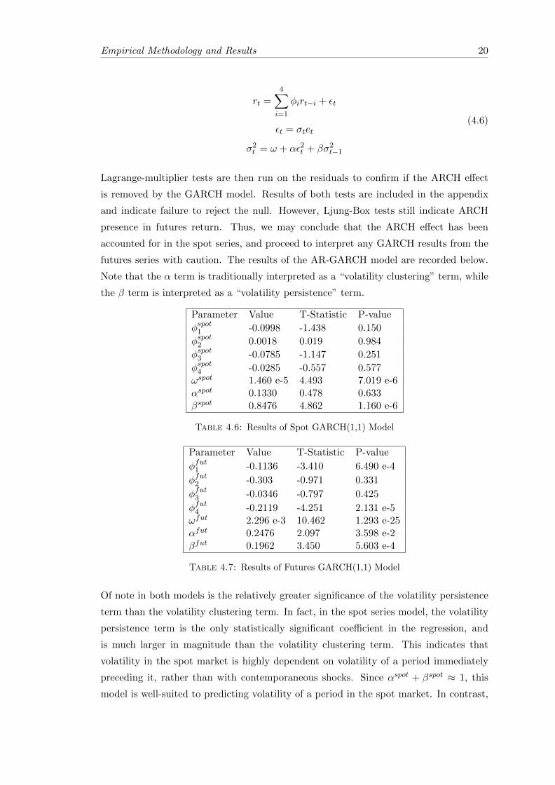
LM Statistic - Spot Series 144.20p-value of Spot Series LM Stat 0.003LM Statistic - Futures Series 9.17p-value of Futures Series LM Stat 0.999

Table 4.5: Results of Lagrange Multiplier Tests

Such test results indicate clearly an ARCH effect in the spot AR(4) model. However,

conflicting results give no clear indication as to the presence of an ARCH effect in the

futures AR(4) model. Thus, a GARCH model will be fitted to both series. Despite the

failure to reject the null of ‘no autocorrelation’ in the futures model, ARCH effects are

common in time series financial return data across asset classes, and we have a strong

prior that the series should exhibit some ARCH effects. This, combined with the result

of the Ljung-Box test, give us reason to fit a GARCH model to the futures series as well.

A GARCH (1,1) model as specified in Bollerslev (1986) and shown below, is selected to

fit the both series. This is due to its parsimonious nature, and a good deal of literature

indicating acceptability to model ARCH processes. Note that the mean model follows

an AR(4) process rather than the constant mean model of Bollerslev.


rt =4∑

i=1

φirt−i + εt

εt = σtet

σ2t = ω + αε2t + βσ2t−1

(4.6)

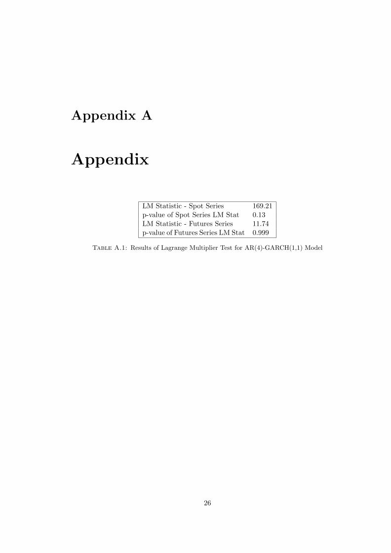
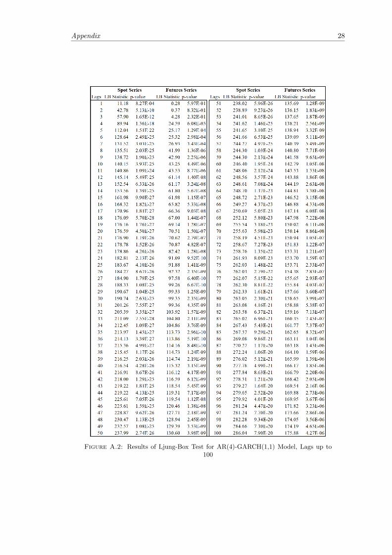
Lagrange-multiplier tests are then run on the residuals to confirm if the ARCH effect

is removed by the GARCH model. Results of both tests are included in the appendix

and indicate failure to reject the null. However, Ljung-Box tests still indicate ARCH

presence in futures return. Thus, we may conclude that the ARCH effect has been

accounted for in the spot series, and proceed to interpret any GARCH results from the

futures series with caution. The results of the AR-GARCH model are recorded below.

Note that the α term is traditionally interpreted as a “volatility clustering” term, while

the β term is interpreted as a “volatility persistence” term.

Parameter Value T-Statistic P-value

φspot1 -0.0998 -1.438 0.150

φspot2 0.0018 0.019 0.984

φspot3 -0.0785 -1.147 0.251

φspot4 -0.0285 -0.557 0.577ωspot 1.460 e-5 4.493 7.019 e-6αspot 0.1330 0.478 0.633βspot 0.8476 4.862 1.160 e-6

Table 4.6: Results of Spot GARCH(1,1) Model

Parameter Value T-Statistic P-value

φfut1 -0.1136 -3.410 6.490 e-4

φfut2 -0.303 -0.971 0.331

φfut3 -0.0346 -0.797 0.425

φfut4 -0.2119 -4.251 2.131 e-5ωfut 2.296 e-3 10.462 1.293 e-25αfut 0.2476 2.097 3.598 e-2βfut 0.1962 3.450 5.603 e-4

Table 4.7: Results of Futures GARCH(1,1) Model

Of note in both models is the relatively greater significance of the volatility persistence

term than the volatility clustering term. In fact, in the spot series model, the volatility

persistence term is the only statistically significant coefficient in the regression, and

is much larger in magnitude than the volatility clustering term. This indicates that

volatility in the spot market is highly dependent on volatility of a period immediately

preceding it, rather than with contemporaneous shocks. Since αspot + βspot ≈ 1, this

model is well-suited to predicting volatility of a period in the spot market. In contrast,


the futures series model is far less predictive. This series exhibits a more statistically

significant coefficient for volatility persistence than for volatility clustering, although

with a smaller magnitude. However, given how [alpha + beta] is not close to 1, the

model is not very predictive and doesn’t seem to do a good job of capturing the volatility

of a period. This, combined with the results of the LB test, indicate that futures price

returns do not follow a process typical of financial assets. This may be a transitory

phase for a completely new asset in a market that is not well-populated yet, or may be

symptomatic of some fundamental characteristic of the asset.

To establish volatility spillover from one market to another, an error-correction model

is conducted on observed volatility. The procedure followed is the same as in our error

correction model in a previous section, which in turn is based on Engle, Granger (1987).

The series upon which the error correction model is conducted is the log of observed

volatility over 2-hour time periods. The results of the regression are below. Note that

σs represents logged observed volatility in the spot series, and σf represents logged

observed volatility in the futures series.

σft − β0 − β1σst = et

∆σst = α1 + δ1εt−1

∆σft = α2 + δ2εt−1

(4.7)

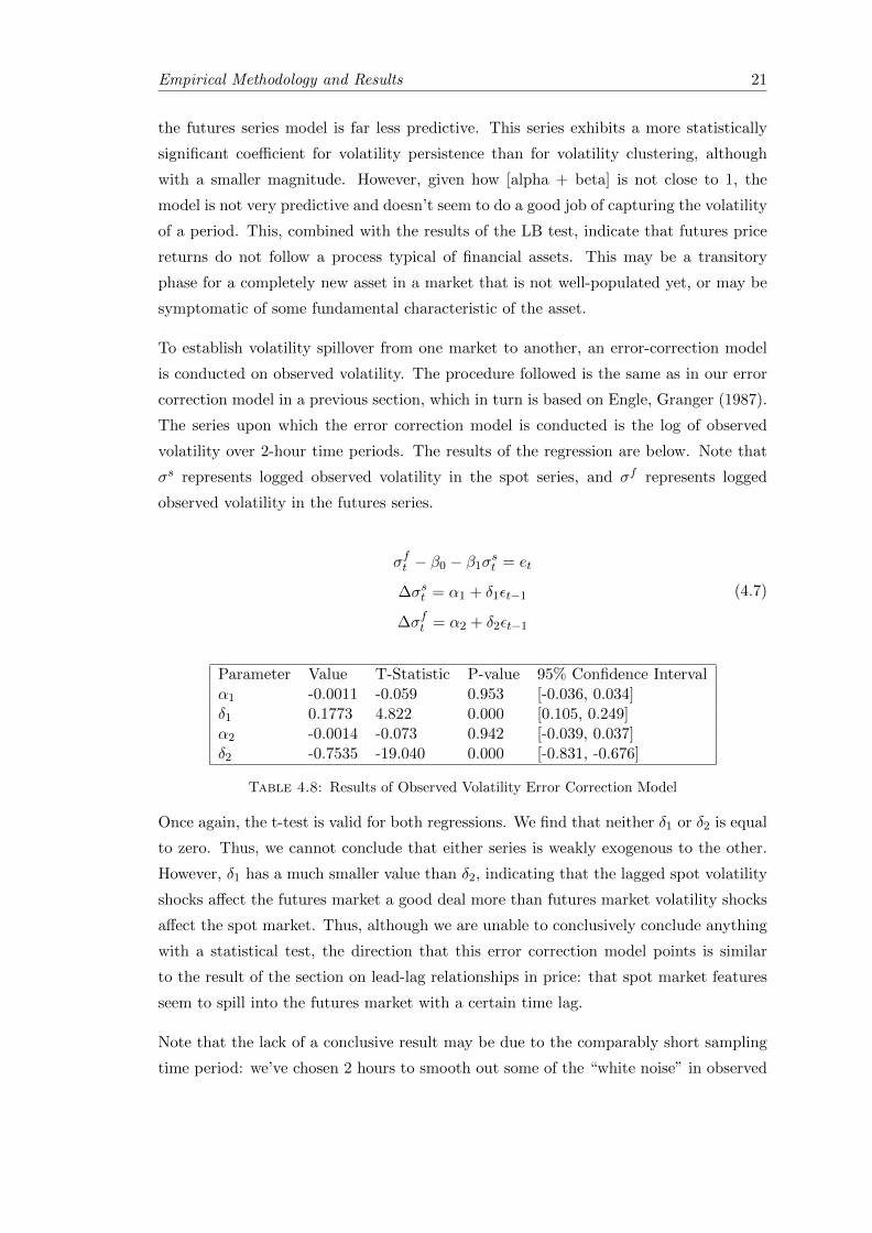
Parameter Value T-Statistic P-value 95% Confidence Intervalα1 -0.0011 -0.059 0.953 [-0.036, 0.034]δ1 0.1773 4.822 0.000 [0.105, 0.249]α2 -0.0014 -0.073 0.942 [-0.039, 0.037]δ2 -0.7535 -19.040 0.000 [-0.831, -0.676]

Table 4.8: Results of Observed Volatility Error Correction Model

Once again, the t-test is valid for both regressions. We find that neither δ1 or δ2 is equal

to zero. Thus, we cannot conclude that either series is weakly exogenous to the other.

However, δ1 has a much smaller value than δ2, indicating that the lagged spot volatility

shocks affect the futures market a good deal more than futures market volatility shocks

affect the spot market. Thus, although we are unable to conclusively conclude anything

with a statistical test, the direction that this error correction model points is similar

to the result of the section on lead-lag relationships in price: that spot market features

seem to spill into the futures market with a certain time lag.

Note that the lack of a conclusive result may be due to the comparably short sampling

time period: we’ve chosen 2 hours to smooth out some of the “white noise” in observed


volatility over short periods of time in relatively illiquid markets. However, both lead-

lag models (of first and second moments) show (to varying degrees) the spot market

leading the futures market, in both first and second moments. That such an effect is

(albeit, more weakly) present in volatility in addition to price more strongly supports

our hypothesis posited in a previous section that information flows may be from the

spot market to the futures market for Bitcoin.

Given support for our hypothesis of the direction of information flows, reasonable follow-

up research would be to examine whether the introduction of futures contracts had any

effect on Bitcoin spot volatility. Given the lack of evidence for information flows from the

futures market to the spot market, the futures market may be functioning inefficiently as

an information transmission mechanism, and actors in the market may not be effectively

intertemporally arbitraging. Much research that supports the introduction of futures as

a stabilizing force for markets is reliant upon an efficient information transmission from

the futures market to the spot market. Given that we do not observe evidence for this

effect, it may be reasonable to assume that the introduction of Bitcoin futures did not

have any significant effect on Bitcoin spot volatility. This is the question we now turn

our attention to.

4.4 Effect of Introduction of Bitcoin Futures on Spot Volatil-

ity

One of the most parsimonious models for measuring effects of a natural experiment-type

event is the difference-in-differences, or DiD model. Such a model is extremely attractive

for its simplicity, its clear assumptions, and results that are easily interpretable. Thus,

in this section, a difference-in-differences model is conducted on Bitcoin. As a control,

three other cryptocurrencies are selected: Ether (or ETH, the cryptocurrency associ-

ated with the Ethereum blockchain), Ripple (or XRP), and Litecoin (or LTC). These

cryptocurrencies are selected because of their strong historical price and volatility cor-

relation to Bitcoin, their susceptibility to similar types of information-shocks as Bitcoin,

and because of their dominance in the cryptocurrency market capitalization rankings.

One of the most important assumptions for the DiD model to provide a valid result is

that the controls would be subjected to the same shocks in the selected time period as

the tested variable, in this case Bitcoin. In other words, all of the selected currencies

must be subjected to all of the same shocks as Bitcoin over the time period selected,

with the only difference being that Bitcoin had futures contracts introduced at some

point in the period. Additionally, all control cryptocurrencies would have to react to all


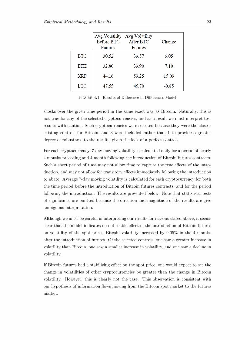
Figure 4.1: Results of Difference-in-Differences Model

shocks over the given time period in the same exact way as Bitcoin. Naturally, this is

not true for any of the selected cryptocurrencies, and as a result we must interpret test

results with caution. Such cryptocurrencies were selected because they were the closest

existing controls for Bitcoin, and 3 were included rather than 1 to provide a greater

degree of robustness to the results, given the lack of a perfect control.

For each cryptocurrency, 7-day moving volatility is calculated daily for a period of nearly

4 months preceding and 4 month following the introduction of Bitcoin futures contracts.

Such a short period of time may not allow time to capture the true effects of the intro-

duction, and may not allow for transitory effects immediately following the introduction

to abate. Average 7-day moving volatility is calculated for each cryptocurrency for both

the time period before the introduction of Bitcoin futures contracts, and for the period

following the introduction. The results are presented below. Note that statistical tests

of significance are omitted because the direction and magnitude of the results are give

ambiguous interpretation.

Although we must be careful in interpreting our results for reasons stated above, it seems

clear that the model indicates no noticeable effect of the introduction of Bitcoin futures

on volatility of the spot price. Bitcoin volatility increased by 9.05% in the 4 months

after the introduction of futures. Of the selected controls, one saw a greater increase in

volatility than Bitcoin, one saw a smaller increase in volatility, and one saw a decline in

volatility.

If Bitcoin futures had a stabilizing effect on the spot price, one would expect to see the

change in volatilities of other cryptocurrencies be greater than the change in Bitcoin

volatility. However, this is clearly not the case. This observation is consistent with

our hypothesis of information flows moving from the Bitcoin spot market to the futures

market.

Chapter 5

Conclusion

All tests seem to provide some level of support for the hypothesis of information flows

from the spot to the futures market. The price Engle-Granger error correction model

establishes a strong positive result of spot price leading futures price. Even though

the observed volatility error correction model does not firmly establish a lead-lag rela-

tionship, when the magnitudes of the relationships are examined, it is clear that spot

observed volatility is a better predictor of futures observed volatility than vice versa.

While we must be careful in the inferences we make from such data, there may be sev-

eral causes that would all merit future research. There may be no advantage held by

traditionally “sophisticated” investors in the futures market that helps them act faster

and on better information than “unsophisticated” actors in the spot market. There

may also be transitory effects as actors in the futures market adjust to trading in a

market for a completely new type of underlying asset. Additionally, behavioral fric-

tions may be somewhat or entirely driving price behavior in the spot market, beyond

an “sophisticated” actors’ abilities to recognize.

Regardless of our inference as to the cause of this phenomenon, it seems likely that

information is flowing from the spot market to the futures market. This is evidenced by

the price lead-lag relationship, in addition to the volatility spillover metrics. Given that

much literature supporting futures markets’ introductions as dampening to volatility or

beneficial to price discovery is contingent on information flows from the futures market

to the spot market, we may infer that the Bitcoin futures market is not functioning

through this channel.

This conclusion does not exclude the existence of some other channel through which

Bitcoin futures may dampen volatility or improve price discovery. However, given the

reliance on information flows in existing theoretical and empirical literature, it seems

24

Appendices 25

likely that the introduction of Bitcoin futures has had no real dampening effect on

volatility. This is confirmed (to some small degree) by the Difference-in-Differences

model, which shows no marked change in observed volatility post-introduction. Given

the relatively young age of the market and of the asset class generally, this will surely

be a topic to be revisited in the coming years.

Appendix A

Appendix

LM Statistic - Spot Series 169.21p-value of Spot Series LM Stat 0.13LM Statistic - Futures Series 11.74p-value of Futures Series LM Stat 0.999

Table A.1: Results of Lagrange Multiplier Test for AR(4)-GARCH(1,1) Model

26

Appendix 27

Figure A.1: Results of Ljung-Box Test for AR(4) Model, Lags up to 100

Appendix 28

Figure A.2: Results of Ljung-Box Test for AR(4)-GARCH(1,1) Model, Lags up to100

Bibliography

[1] Frank Asche and Atle Guttormsen. Lead lag relationships between futures and

spot prices. Institute for Research in Economics and Business Administration

Working Paper Series, (2), 2002.

[2] Dirk G. Baur, Thomas Dimpfl, and Konstantin Kuck. Bitcoin, gold, and the us

dollar – a replication and extension. Finance Research Letters, 2017.

[3] Tim Bollerslev. Generalized autoregressive conditional heteroskedasticity. Journal

of Econometrics, 52, 1986.

[4] George E. P¿ Box and David A. Pierce. Distribution of residual autocorrelation in

autoregressive integrated moving averagee time series models. Journal of

American Statistical Association, 65(332), 1970.

[5] Morten Brandvold, Peter Molnar, Kristian Vagstad, and Ole Christian Andreas

Valstad. Price discovery on bitcoin exchanges. Journal of International Financial

Markets, Institutions, and Money, 2015.

[6] Kalok Chan, K. C. Chan, and G. Andrew Karolyi. Intraday volatility in the stock

index and stock index futures markets. The Review of Financial Studies, 4(4),

1991.

[7] V. V. Chari, Ravi Jagannathan, and Larry Jones. Price stability and futures

trading in commodities. Quarterly Journal of Economics, 104, 1990.

[8] Gerald P. Dwyer. The economics of bitcoin and similar private digital currencies.

Journal of Financial Stability, 17, 2015.

[9] Annie H. Dyhrberg. Bitcoin, gold, and the dollar – a garch volatility analysis.

Finance Research Letters, 16, 2016.

[10] Robert F. Engle, Takatoshi Ito, and Wen-Ling Lin. Meteor showers or heat

waves? heteroskedastic intra-day volatility in the foreign exchange market.

Econometrica, 58(3), 1990.

29

Bibliography 30

[11] David S. Evans. Economic aspects of bitcoin and other decentralized public-ledger

currency platforms. Coase-Sandor Institute for Law and Economics Working

Paper Series, (685), 2014.

[12] Milton Friedman. The case for flexible exchange rates. Essays in Positive

Economics - Chicago University Press, 1953.

[13] Florian K. Glaser, Kai Zimmermann, Martin Haferkorn, Moritz C. Weber, and

Michael Siering. Bitcoin – asset or currency? revealing users’ hidden intentions.

Proceedings of the European Conference on Information Systems (ECIS), 2014.

[14] Stewart Hodges. Do derivative instruments increase market volatility? Options:

Recent Advances in Theory and Practice II, 1992.

[15] Masahiro Kawai. Price volatility of storable commodities under rational

expectations in spot and futures markets. International Economic Review, 24(2),

1983.

[16] Steward Mayhew. The impact of derivatives on cash markets: What have we

learned? 1999.

[17] John Stuart Mill. Principles of Political Economy. Google Books, 1871.

[18] Anne E. Peck. Futures markets, supply response, and price stability. Quarterly

Journal of Economics, 90, 1976.

[19] Commodity Futures Trading Commission Market Reports. Current traders in

financial futures reports, futures only (long form), Mar 2018.

[20] Commodity Futures Trading Commission Market Reports. Traders in financial

futures reports - explanatory notes, Mar 2018.

[21] Alexander H. Sarris. Speculative storage, futures markets, and the stability of

commodity prices. Economic Inquiry, 22(1), 1984.

[22] George Selgin. Synthetic commodity money. Journal of Financial Stability, 17,

2015.

[23] Param Silvapulle and Imad A. Moosa. The relationship between spot and futures

prices: Evidence from the crude oil market. The Journal of Futures Markets,

19(2), 1999.

[24] Adam Smith. The Wealth of Nations. Google Books, 1776.

[25] Standards and Poors Global. Sp dow jones indices – sp 500, Mar 2018.

Bibliography 31

[26] George P. Tsetsekos and Panos Varangis. The structure of derivatives exchanges:

Lessons from developed and emerging markets. World Bank Policy Research


[27] Stephen J. Turnovsky. The determination of spot and futures prices with storable

commodities. Econometrica, 51(5), 1983.

[28] Robert Viglione. Does governance have a role in pricing? cross-country evidence

from bitcoin markets. SSRN Electric Journal, 2015.

[29] Holbrook Working. Theory of the inverse carrying charge in futures markets.

Journal of Farm Economics, 30, 1948.

[30] David Yermack. Is bitcoin a real currency? an economic appraisal. NBER


information and volatility dynamics in the bitcoin futures...

Documents