inflation targeting and real exchange rates in emerging … · nber working paper series inflation...
TRANSCRIPT

NBER WORKING PAPER SERIES
INFLATION TARGETING AND REAL EXCHANGE RATES IN EMERGING MARKETS
Joshua AizenmanMichael Hutchison
Ilan Noy
Working Paper 14561http://www.nber.org/papers/w14561
NATIONAL BUREAU OF ECONOMIC RESEARCH1050 Massachusetts Avenue
Cambridge, MA 02138December 2008
We thank Mahir Binici, Nan Geng, Gurnain Kaur Pasricha and Kulakarn Tantitemit for helpful researchassistance and to Scott Roger and Mark Stone for providing data. We are grateful to two anonymousreferees of this journal for helpful comments. We also thank participants of the Research Seminarof the IMF, especially Herman Kamil; participants of the Third NIPFA-DEA Program Meeting onCapital Flows Conference in New Delhi, especially our discussant Vincent Coen; and participantsat a seminar at the University of Victoria, Canada, for helpful comments. The views expressed hereinare those of the author(s) and do not necessarily reflect the views of the National Bureau of EconomicResearch.
NBER working papers are circulated for discussion and comment purposes. They have not been peer-reviewed or been subject to the review by the NBER Board of Directors that accompanies officialNBER publications.
© 2008 by Joshua Aizenman, Michael Hutchison, and Ilan Noy. All rights reserved. Short sectionsof text, not to exceed two paragraphs, may be quoted without explicit permission provided that fullcredit, including © notice, is given to the source.
Inflation Targeting and Real Exchange Rates in Emerging MarketsJoshua Aizenman, Michael Hutchison, and Ilan NoyNBER Working Paper No. 14561December 2008, Revised July 2010JEL No. E52,E58,F15,F3
ABSTRACT
We investigate inflation targeting (IT) in emerging markets, focusing on the role of the real exchangerate and the distinction between commodity and non-commodity exporters. IT emerging markets appearto follow a “mixed strategy” whereby both inflation and real exchange rates are important determinantsof policy interest rates. The response to real exchange rates, however, is more constrained than in non-ITregimes. We also find that the response to real exchange rates is strongest in those countries followingIT policies that are relatively intensive in exporting basic commodities; and present a theoretical modelthat explains these empirical results.
Joshua AizenmanDepartment of Economics; E21156 High St.University of California, Santa CruzSanta Cruz, CA 95064and [email protected]
Michael HutchisonDepartment of EconomicsE2University of CaliforniaSanta Cruz, CA [email protected]
Ilan NoySaunders Hall 5422424 Maile WayUniversity of Hawaii, ManoaHonolulu, HI [email protected]
1
1. INTRODUCTION
Inflation targeting is becoming a standard operating procedure for central banks
around the world. By mid 2008, most central banks in the OECD countries1 and a
growing number of developing economies had adopted inflation targeting. There is no
international coordination to promote this monetary regime change, and countries do not
join an internationally recognized monetary system nor follow common “rules of the
game.” Adopters of inflation targeting do so primarily because of the framework’s
perceived success in delivering low and stable inflation.
Despite its popularity, there is substantial controversy and mixed empirical
evidence in the evaluation of the inflation-targeting framework. There are two main
empirical approaches. The first approach focuses on the macroeconomic outcomes of
countries following inflation-targeting regimes as compared to non-targeting countries.
Although few argue that inflation targeting has harmful effects, there remains a vigorous
academic and policy debate over whether the adoption of this monetary regime in
advanced industrial countries has contributed to substantial declines in average inflation,
lower inflation volatility and general macroeconomic stability compared to those
countries not following inflation-targeting rules.2
The second empirical approach evaluating inflation-targeting (IT) policies focuses
on central bank behavior under inflation targeting and non-targeting and how they
operate in an IT environment. Even in this strand of the literature there is mixed evidence
over whether formal adoption of an inflation targeting regime substantively changes the
behavior of central banks, and in particular their responses to inflation and output gaps.
2
This paper investigates the empirics of inflation targeting in emerging market
economies within the context of the second strand of the literature—central bank
operating behavior. We focus in particular on emerging-market central banks’ responses
to inflation, output gaps and real exchange rates using Taylor rule models (as in Clarida
et al., 1998). Our aim is to distinguish between episodes when central banks are
committed to an explicit inflation-targeting monetary regime and those periods of time
when they are not (including central banks that have never followed inflation targeting).
We focus on two factors critical to the conduct and control of monetary policy in
emerging markets—wide swings in the real exchange rate and the extent to which the
countries are concentrated in commodity exports. We demonstrate, in the context of a
simple illustrative model, that these distinguishing characteristics are in principle
important in designing the form of the monetary policy rule. For a commodity exporting
country that is vulnerable to terms-of-trade shocks, in particular, when experiencing large
real exchange rate shocks that can affect potential output a modified version of inflation
targeting dominates a pure inflation targeting strategy.
Our empirical work is based on panel-data so as to distinguish between group
characteristics, respectively, of the inflation-targeting and non-targeting central banks in
emerging markets and further between commodity exporting inflation targeters from
other IT regime countries. We characterize inflation targeting strategies in the context of
a modified Taylor rule operating procedure, and demonstrate that this rule varies
markedly from non-targeting emerging markets (as well as inflation-targeting industrial
countries). Moreover, our focus is on the role of the real exchange rate in the policy rule

3
and how this is affected by the countries’ exposure to commodity-intensive production
(and, hence, terms-of-trade shocks).
Four factors motivate our empirical research. Firstly, the great bulk of the
research in this area is concerned with inflation targeting in advanced industrial countries
and relatively less research addresses the particular features of inflation targeting in
emerging markets3. There are many reasons that emerging markets may differ from
industrial countries in the approach to inflation targeting. These reasons include different
institutional arrangements, especially those relating to the credibility and political
independence of the central bank, different inflation and macroeconomic histories,
different exposures to terms-of-trade shocks, and different levels of financial
development. Aghion et al. (2006) demonstrate that countries with relatively less
developed financial sectors are more likely to suffer output losses associated with
exchange rate volatility. In this case, greater concern for real exchange rate volatility may
lead central banks in emerging markets—countries with lower levels of financial
development than industrial countries—to follow a monetary policy rule (Taylor rule)
that captures some form of target inflation, output deviations from the natural rate and
real exchange rate fluctuations.
Secondly, our emphasis is on introducing real exchange rate fluctuations into the
inflation-targeting framework. Real exchange rates are likely to play an important role in
the formulation of optimal monetary policy in emerging markets, as shown theoretically
in our illustrative model (appendix A), and we examine this connection in our estimations
of de facto policy rules.
4
Thirdly, the distinction between heavily concentrated commodity-exporting
emerging markets and non-concentrated emerging markets is potentially important in
how inflation targeters work in practice. This difference accounts for different
vulnerability to terms-of-trade shocks. We explore this distinction.
Fourthly, we follow a panel methodological approach in examining these issues.
Most other studies in this area have relied upon individual country time-series analysis. A
panel analysis provides some advantages since it allows clear focus on characteristics of
policy rules common to inflation-targeting countries treated as a group and allows us to
distinguish them from non-inflation targeting countries.
Our results indicate that the publically announced adoption of inflation targeting
strategies by central banks in emerging markets, often with much fanfare, is a substantive
deviation from past monetary policy formulation and sharply different from non-targeting
emerging markets. As our theoretical model predicts, however, inflation targeting
emerging markets are not following “pure” inflation targeting strategies. Rather, we find
that external variables play a very important role in the policy rule— inflation-targeting
central banks in emerging markets systematically respond to the real exchange rate. Of
the inflation targeting group, those with particularly high concentration in commodity
exports change interest rates much more pro-actively to real exchange rate changes than
do the non-commodity intensive group. Overall, our results are robust to a variety of
model formulations and estimation strategies.
The next section discusses the inflation targeting literature as it applies to
emerging markets, and highlights the gap in the empirical literature which we address in
our contribution. Section 3 presents the data, descriptive statistics and empirical model.
5
Section 4 presents the empirical results and section 5 concludes. Appendix A presents the
theoretical model that motivates our empirical formulation of the policy rule equations.
2. INFLATION TARGETING IN EMERGING MARKETS
There is a large empirical literature on inflation targeting, most of which focuses
on advanced industrial countries. These studies generally take one of two approaches.
The first approach measures the effects of inflation targeting on inflation, inflation
volatility, and other macroeconomic variables. The second approach focuses on
characterizing central bank operating procedures, attempting to distinguish between
policy functions of inflation targeting countries and those not targeting inflation. Studies
in the first strand of the empirical literature employ both individual country time-series
and multi-country panel methods, while the second strand of literature is almost
exclusively focused on individual country time-series.
(a) Macroeconomic effects of inflation targeting
Empirical studies generally find mixed results on the effects of inflation targeting
on inflation and other macroeconomic variables. For example, Johnson (2002) undertakes
a panel study consisting of five IT (Australia, Canada, New Zealand, Sweden and the
United Kingdom) and six non-IT advanced industrial countries. He finds that the
announcement of inflation targets materially lowers expected inflation (controlling for
business cycle effects, past inflation and fixed effects). Also in the context of a panel
regression framework, Mishkin and Schmidt-Hebbel (2007) similarly conclude that
inflation targeting does make a difference in advanced industrial countries by helping
them achieve lower inflation in the long run and have smaller inflation responses to oil
and exchange rate shocks. However, the results for advanced country inflation-targeters

6
are very similar to their high-performing country control group.4 Rose (2007) argues that
inflation targeting is a very durable (long-lasting) regime compared to other monetary
regimes and that inflation targeters have both lower exchange rate volatility and less
frequent “sudden stops” of capital flows. By contrast, Ball and Sheridan (2005), in a
cross-section investigation, reject any long-term differences between advanced industrial
inflation targeters (seven countries) and non-targeters (thirteen countries).
The experience and relative success of emerging markets with inflation targeting
is somewhat more supportive, although this remains controversial. Mishkin and Schmidt-
Hebbel (2007) find that inflation targeting in emerging countries performs less well than
in advanced industrial countries, although the pre- and post-inflation targeting reductions
in inflation in emerging markets are substantial.5 The IMF (2005), using the methodology
of Ball and Sheridan (2005), presents results of a study focusing on 13 emerging market
inflation targeters compared with 29 other emerging markets. They report that inflation
targeting is associated with a significant 4.8 percentage point reduction in average
inflation, and a reduction in its standard deviation of 3.6 percentage points relative to
other monetary strategies.
Gonçalves and Salles (2008) and Lin and Ye (2009), using different
methodologies, reach similar conclusions to the IMF study; they find that adoption of an
inflation targeting regime leads to lower average inflation rates and reduced volatility
compared to a control group of non-targeters. A recent edited volume on inflation
targeting in emerging markets, focusing mainly on individual country case studies, also
finds quite positive outcomes associated with the adoption of IT regimes (De Mello,
2008). In contrast, a more recent paper argues that once common time trends are

7
accounted for, this positive benefit of IT regimes disappears and even argues that the
disinflation period is potentially more recessionary under IT (Brito and Bystedt, 2010).
(b) Policy functions in IT regimes
In terms of central bank policy functions, Clarida, Gali and Gertler (1998) focus on
six major industrial countries and suggest that the G3 (Germany, Japan and U.S.) have
followed an implicit form of inflation targeting since 1979. The main evidence for this
conclusion is that these central banks are forward looking, and respond to anticipated as
opposed to lagged inflation. Clarida et al. (1998) argue that the success of the G3 in
lowering inflation and keeping inflation at a low level may be attributable to this implicit
inflation-targeting policy. They conclude that inflation targeting may be superior to fixing
exchange rates as a nominal anchor (as was prevalent in their sample period for the G3
countries of France, Italy and the United Kingdom). They found the response to real
exchange rates is significant and of the expected sign, but small in magnitude for
Germany and Japan.
Other studies have investigated differences in IT and non-IT policy regimes by
explicitly estimating “Taylor rule” equations for individual countries. A number of
studies in this genre, focusing on advanced industrial countries, find some evidence that
countries are following significantly different policy rules in IT regimes (e.g. Mohanty
and Klau, 2005; Edwards, 2006; Corbo et al., 2001). For example, Corbo et al. (2001)
find somewhat mixed evidence for seventeen OECD countries estimated individually.
They find that inflation targeters exhibit the largest inflation gap coefficient (response to
inflation) relative to the output gap coefficient (response to output), although in most
cases the coefficients are not statistically different from zero. Lubik and Schorfheide
8
(2007) estimate a calibrated small-scale GE model for a small open economy using data
for Australia, Canada, New Zealand and the United Kingdom over 1983 to 2002
(quarterly data). They consider Taylor-type rules, where the authorities respond to output,
inflation and exchange rates. They find that Australia and New Zealand change interest
rates in response to exchange rate movements, but that Canada and the United Kingdom
do not respond to exchange rates.
Dennis (2003) investigates several models for the Australian experience and finds
that the authorities should optimally focus not just on inflation but also on real exchange
rate fluctuations and terms of trade when they set interest rates to the extent that import
goods are consumption goods (and enter into CPI). Ravenna (2008) considers the
Canadian case with IT targeting. He estimates a DSG model and is able to determine
whether the good inflation performance of Canada since adopting an IT regime is due to
the IT policy or to “good luck.” He finds that low average inflation since adopting the IT
regime is associated with the credibility of policy under this regime. However, the lower
volatility of inflation is mainly associated with “good luck” in that few major adverse
shocks have impacted the Canadian economy during this period.
Other studies suggest that monetary policy operating procedures do not
fundamentally change with the move to an IT regime. Drueker and Fischer (2006), for
example, find “no difference” in the monetary policy rules followed by IT countries and
comparable non-IT countries in their own empirical work, and at best mixed evidence
supporting any substantive difference in numerous studies in their survey of the subject.
They estimate individual country time-series regressions and compare high-performing
advanced industrial countries that are following an IT regime and those that are not. A
9
more recent contribution that attempts to explain this indifference, concludes that
inflation targeting is not a binary choice and develops an index for measuring the ‘extent’
of inflation targeting pursed by the monetary regime (Miao, 2009).6
(c) Policy rules, real exchange rates and commodity export concentration
Only a few empirical studies focus on central bank reaction functions in emerging
markets, and this is done on a case by case basis. Schmidt-Hebbel and Werner (2002)
apply common empirical framework (VAR models) to compare the experiences of Brazil,
Chile and Mexico with inflation targeting. They estimate Taylor rule equations for each
country with the real interest rate as the dependent variable. Only for Brazil is the
expected inflation gap statistically significant, whereas only for Chile is the output gap
statistically significant. They do find that the trade surplus (lagged) enters negatively and
significantly in most cases (i.e. trade surplus leads to decline in real interest rate) and that
this effect dominates all other variables. They find that these countries continue to
respond to exchange rate changes in the short-term, if not the medium-term, and
characterize them as “dirty” floaters.7
Corbo et al. (2001) estimate Taylor-rule type equations for eight emerging-market
economies over 1990-1999 using quarterly data. They classify countries during the 1990s
as IT, potential IT and non-IT.8 Two emerging markets are in their IT category (Chile and
Israel), five are in the potentially targeting category (South Africa, Brazil, Colombia,
Mexico and Korea) and one is in the non-IT category (Indonesia). In the IT and potential
IT categories, four (two) central banks appear to respond to inflation (output) deviations
from target in setting interest rates. The authors do not test, in their Taylor rule estimates,
whether central banks in emerging markets consider external variables.

10
Mohanty and Klau (2004) estimate modified Taylor rules for 13 emerging market
and transition economies, complementing inflation, the output gap and lagged interest
rates with current and lagged real exchange rate changes. They find that the coefficients
on real exchange rate changes are statistically significant in ten countries (OLS
estimates), with the significant contemporaneous effect ranging from -0.33 (Brazil) to
0.35 (Chile). The policy response to exchange rate changes is frequently larger than the
response to inflation and the output gap. They conclude that this supports the “fear of
floating” hypothesis. Mohanty and Klau (2004) do not explicitly address the inflation
targeting issue in this context, but it is apparent that these countries, whether or not they
profess to follow an IT regime, are attempting to stabilize real exchange rates as well as
control inflation and stabilize output.
Edwards (2006) investigates the determinants of the exchange rate response in the
Taylor-rule regressions, building on the work by Mohanty and Klau (2004). He runs
cross-country regressions of the exchange rate coefficient on several explanatory
variables (each regression with 13 observations). Edwards (2006) finds that countries
with a history of high inflation, and with historically high real exchange rate volatility,
tend to have a higher coefficient (response) to the real exchange rate in Taylor rule
equations, yet he does not distinguish the degree of exposure to terms-of-terms shocks
that is especially large for commodity exporting countries.
De Mello and Moccero (2008) estimate interest rate policy rules for four Latin
American emerging markets—Brazil, Chile, Colombia and Mexico—characterized by
inflation targeting and floating exchange rates in 1999. They estimate an interest rate
policy function in the context of a New Keynesian structural model with equations for
11
inflation, output and interest rates. They find inflation targeting, in a post-1999 regime,
has been associated with stronger and persistent responses to expected inflation in Brazil
and Chile. Mexico is the only country they find where changes in nominal exchange rates
were found to be statistically significant in the central bank’s reaction function during the
IT period.
Taking a different approach, Ball and Reyes (2004 and 2008), compare IT
regimes to the Fear-of-Floating policy pursed by many countries. They conclude that
these are distinctly different regimes and that the IT regimes are more similar (in terms of
the behavior of interest rates, exchange rates, and other variables) to floating regimes
than to the fear-of-floating ones.
(d) Importance of real exchange rates for IT regimes
The theoretical importance of the real exchange rate to the conduct of monetary
policy in an IT regime is presented in appendix A. We illustrate these considerations in a
simplified version of Ball (1999), where the policy maker is concerned about real
exchange rate volatility.9 The wish to mitigate exchange rate volatility follows the logic
of Aghion et al. (2009), who show that exchange rate volatility reduces productivity in
developing countries, attributing it to financial channels. Aghion et al. (2009) find that
the adverse effects of exchange rate volatility are larger for the less financially developed
countries. These adverse effects are significant for practically all the emerging markets
and developing countries, which are the focus of our paper.10 Importantly, their study
used data prior to the 2008-9 crisis, a crisis that vividly illustrated that even emerging
markets with high levels of financial development (as measured, for example, by the ratio

12
of private credit to GDP) have been heavily exposed to the adverse repercussions of
exchange rate volatility.11
The adverse effect of volatility may be the outcome of increasing the expected
cost of funds in circumstances where agency and contract enforcement costs are
prevalent, the financial system is shallow, and trade openness is significant.12 These
conditions tend to be exacerbated in developing countries relying heavily on mineral and
other commodity exports. Our simulated model, as presented in figure 1A of the
appendix, confirms that a greater weight on mitigating exchange rate volatility tends to
increase the responsiveness of the policy rule to exchange rate changes, possibly with
sizable welfare effects.13
Our focus is on the short run stabilization of the real exchange rate, where the
policy maker presumes, short of better information, that the equilibrium REER is highly
persistent, thus most of the short run shocks may reflect transitory disturbances. This
presumption reflects both the persistency of the REER, and the wide standard errors
associated with predicting equilibrium exchange rates (see further discussion in
Eichengreen, 2007).
There are, of course, other possible reasons why a central bank pursing an IT
strategy will choose to also concern itself with the exchange rate. This is true especially
in emerging markets given their shallow currency markets, their short-history of stable
inflation, the importance of the exchange rate as an anchor for expectations and the
possibility of currency mismatch exposure in strategically important sectors (see Amato
and Gerlach, 2002). In a recent more analyitical work, Pavasuthipaisit (2010) develops a

13
DSGE model that also concludes that IT regimes should respond to the exchange rate
shocks under certain conditions that the paper outlines.
Given these considerations, we test the degree to which the policy rule adopted by
IT commodity-intensive developing countries differs from that of the IT non-commodity
exporters, finding support to the greater sensitivity of commodity IT countries to
exchange rate changes.14
3. DATA
As we detail in the introduction, our focus is on emerging markets. We classify
emerging markets using the list of countries included in Morgan Stanley’s MSCI
Emerging Markets Index. The 16 countries in our dataset are: Argentina, Brazil,
Colombia, Czech Republic, Hungary, Indonesia, Israel, Jordan, Korea, Malaysia, Mexico,
Morocco, Peru, Philippines, Poland and Thailand (Appendix B)15. The data sample was
restricted by using quarterly data (annual data provides a much larger group of countries)
and by countries that use nominal interest rates as a primary operating instrument of
monetary policy.
We rely on Mishkin and Schmidt-Hebbel (2007) to identify the monetary regime
and the exact start date of inflation targeting though the IT start dates given by Rose
(2007) are almost identical. We collect quarterly data for these 16 emerging market
countries for 1989Q1 to 2006Q4 - transition economies only have available data starting
in the beginning of the 1990s. We delete from our dataset hyperinflationary periods
(annual inflation higher than 40%). Our primary source for data is the IMF’s International
Finance Statistics CD-ROM, more details are provided in the data appendix (Appendix
C).

14
4. METHODOLOGY AND RESULTS
(a) Preliminaries
Table 1 describes the main variables we examine and their descriptive statistics
for our sample of emerging markets. The first column shows the mean and standard
deviation for those country-quarter observations in which an inflation-targeting regime
was in place. The second column includes the sample of observations consisting of
countries who never adopted an IT regime and IT countries before their adoption of an IT
regime.
[table 1 here]
GDP growth is virtually the same in the IT and non-IT samples, while inflation is
about half of the level on average in IT regimes (5.4 percent) compared to non-IT
regimes (9.6 percent). The average level of nominal interest rates is 3.7 percentage points
less in the IT sample compared with the non-IT sample, a somewhat smaller difference
than the 4.2 percentage point difference in inflation rates between the two regimes,
indicating somewhat higher average short-term real interest rates in the IT sample.
The external variables indicate that IT emerging markets appear to experience a
substantially higher rate of average depreciation of the real exchange rate and lower rate
of international reserve accumulation. This suggests less exchange rate management on
the part of the IT countries. Due to the large variability of the sample observations,
however, none of these differences are statistically significant using standard thresholds.
In order to examine the time-series properties of our data and assess the
appropriate estimation methodology we conduct panel unit root tests (Appendix D). We
15
employ the panel unit root tests described in Levin et al. (2002) and Breitung (2000) and
reject unit roots for all of our time series using at least one or both of these tests.16
(b) Taylor Rule Regression Results
Following an extensive literature that originates from Taylor (1993), we assume a
monetary policy reaction function of the following form:
* *1 ( ) ( )t t t t ti i y y Xρ α β π π γ−= + − + − + (1)
As is standard in this literature, we assume the authorities, in setting the policy interest
rate, react to both the output gap and the inflation gap. In addition, following English et
al. (2002), we assume a policy smoothing goal that manifests in a lagged interest rate on
the RHS. The main focus of this paper, however, are a set of possible external variables
( tX ) that may also be part of the policy reaction function. Our estimation equation for a
panel of 16 emerging-market countries is:
, , 1 , , , ,( )i t i i t i t i i t i t i ti i y y Xμ ρ α βπ γ ε−= + + − + + + (2)
The inflation target variable ( *π ) is assumed to be time invariant for each country and is
subsumed in the country fixed-effect ( iμ ) parameter.
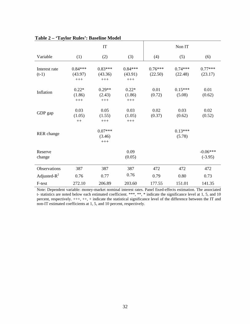
Table 2 presents the estimates for the benchmark Taylor rule regressions
employing a fixed-effects least-squares estimation procedure (LSDV).17 Column (1) and
(4) presents the benchmark model without external variables for the IT and non-IT
samples, respectively. The other columns extend the benchmark to the external variables.
Columns (2) and (5) combine the benchmark model with the percentage change in the

16
real exchange rate, and columns (3) and (6) combine the benchmark model with the
percentage change in international reserve holdings.
[table 2 here]
The model explains much of the variability in interest rates, with explanatory
power ranging from 73-80% (adjusted R2). The degree of persistence, measured by the
lagged interest rate coefficient, is quite high. The persistence in the IT group is
marginally higher than in the non-targeting group. The coefficient on inflation is highly
significant, large and stable (with a narrow 0.22-0.29 range) in the inflation-targeting
regime but not generally in the non-IT regime. Given the estimated impact effects and
persistence, the long-term response for the IT targeters to a one percentage point rise in
inflation is to increase interest rates by between 1.4-1.7 percentage points. Non-IT
policymakers do not respond to inflation rates in the same pronounced and significant
way that their IT counterparts do, i.e. the impact response of 0.15 implies a 0.58
percentage point long-term response in the non-IT group. The output gap is not
significant in any of the regressions.18
The external variables are also very important in distinguishing the operating
procedures of the IT and non-IT groups. Both IT and non-IT emerging market central
banks respond to real exchange rates in setting interest rates-- the coefficients are large
and highly statistically significant. It is noteworthy, however, that the real exchange rate
response is much smaller in the IT countries (0.07) compared to the non-IT countries
(0.13). The IT group attempts to “lean against the wind” and stabilize the exchange rates
by increasing interest rates in response to real exchange rate depreciation, but their
actions are apparently more constrained by the commitment to target inflation than the
17
non-IT group in how proactively this objective is pursued. In a similar vein, it is only the
non-IT group that takes into account changes in international reserves in setting interest
rates. In particular, a one percent increase in reserves leads to a 6 basis point decline in
domestic short-term interest rates for non-IT countries (23 basis point long-run effect).
Only the non-IT group eases policy in response to international reserve inflows.19
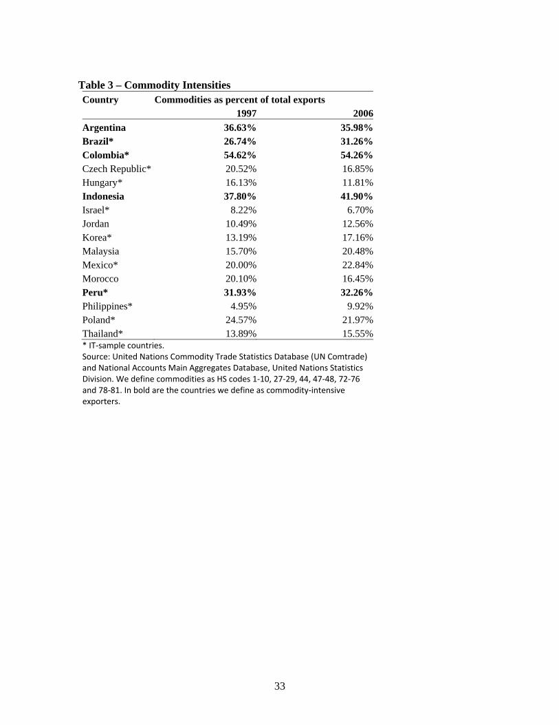
(c) Commodity Exporters
Our theoretical discussion emphasizes the critical role of “external vulnerability”
in the setting of policy interest rates in emerging markets. External vulnerability in turn is
likely to be magnified if countries are significant commodity exporters. These countries
are much more vulnerable to terms-of-trade shocks and real exchange rate shocks,20 and
would presumably place greater emphasis on stabilizing the real exchange rate when they
set interest rates.
[table 3 here]
To address this issue, we divide our IT sample into commodity exporters and non-
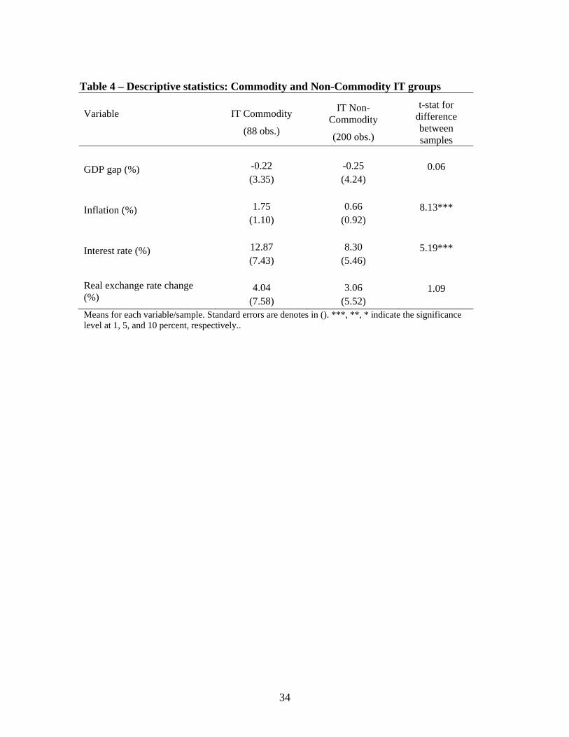
commodity exporters. Summary statistics for the commodity exporting and non-
commodity exporting IT countries are reported in Table 4 and policy equations are
reported in Table 5. Average inflation is higher and interest rates are substantially higher
in the commodity-exporting group, while the other variables of interest are quite similar
to the non-commodity exporting group. In particular, the mean GDP gap and mean real
exchange rate changes are not significantly different between the two groups.
[table 4 here]

18
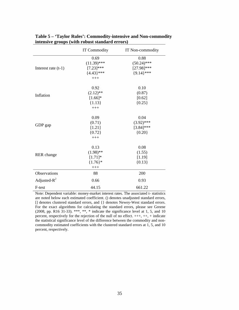
The interest rate policy equation estimates, as theory suggests, are very different
for the commodity and non-commodity IT countries. In particular, shown in Table 5, the
commodity-intensive exporting countries follow a much stronger leaning-against-the-
wind exchange rate policy.21 The real exchange rate response (point estimate) is
statistically significant and positive only in the commodity-intensive countries; and the
degree of response is almost twice as large as in the non-commodity group. In particular,
ten percent depreciation in the real exchange rate causes the commodity-intensive central
banks to increase short-term interest rates by 130 basis points, while the non-commodity
central banks increase interest rates by 80 basis points.
[table 5 here]
Surprisingly, only the commodity-intensive countries appear to be following an
IT policy—despite the two samples including only IT observations. In particular, the
response to inflation is only significant in the commodity-intensive group equation. The
point estimate indicates that a one percent rise in inflation leads to an 92 basis point
increase in the nominal interest rate. The response of the non-commodity exporting group
to inflation, despite an official IT policy regime, is not statistically significant.
It is noteworthy that the strong response to inflation of the commodity-intensive
IT group, and apparently weak response of the non-commodity intensive group, is
probably not because they have radically different histories of inflation or credibility.
That is, we do not think the differences in results are because the non-commodity IT
group are “superior” inflation targeters, with so much credibility with the public that
they do not need to respond to short-term fluctuations in inflation. In particular, the

19
inflation rate of the non-commodity IT group is 4.8 percent, lower than the commodity IT
group average but nonetheless substantial.22
Several recent papers have pointed out that estimations of fixed-effects panels should
also consider more robust ways to estimate the standard errors in finite samples (e.g.,
Petersen, 2009). Since table 5 presents our key results, we follow the suggestions in
Kézdi (2004) and Petersen (2009) and estimate the model with clustered standard
errors.23 Petersen (2009), however, also finds the Newey-West estimator to be superior in
some models. In order to establish the robustness of our results, we therefore estimate the
specifications in table ) with both these standard-errors estimators. We present these
results and show that while the standard errors indeed increase (and statistical
significance therefore decreases), our conclusions regarding the tendency of IT
commodity intensive emerging markets to respond to the changes in exchange rate when
setting the interest rate as robust.
(d) Simultaneity and Varying Inflation Targets
Policy-rule estimation in a panel-setting with lagged dependent variables may
lead to estimation bias. We deal this issue by following the Hausman and Taylor (1981)
estimation procedure. This procedure takes into account bias in estimation of panels with
predetermined and/or endogenous variables.
Moreover, the estimates of equation (2) that we have presented thus far have
implicitly assumed that that the inflation targets were constant in every IT country. Since
in many cases the inflation target was reduced over time, this may lead to biased
estimates. We address this issue by substituting inflation by deviations of inflation from
the actual inflation target as stated by the monetary authority.24
20
The Hausman-Taylor (H-T) three-step estimation methodology is an instrumental
variable estimator that takes into account the possible correlation between the disturbance
term and the variables specified as predetermined/endogenous. The methodology requires
distinguishing between those control variables that are assumed to be (weakly) exogenous
and those that are assumed to be predetermined/endogenous and thus correlated with the
country specific effects. We assume that only the GDP gap variable is exogenous.
In the first step of the H-T estimation, estimates from a country-fixed-effects
model are employed to obtain consistent but inefficient estimates for the variance
components for the coefficients of the time-varying variables. In the second step, an
FGLS procedure is employed to obtain variances for the time-invariant variables. The
third step is a weighted IV estimation using deviation from means of lagged values of the
time-varying variables as instruments. The exogeneity assumption requires that the
means of the exogenous variables will be uncorrelated with the country effects.25
Under the plausible exogeneity assumption described above, the H-T procedure
provides asymptotically consistent estimates for dynamic panels, but it is not the most
efficient estimator possible. More efficient GMM procedures rely on utilizing more
available moment conditions to obtain a more efficient estimation (e.g., Arellano and
Bond, 1991). These, however, are typically employed in estimation of panels with a large
number of individuals and short time-series and in our case of small-N large-T the
number of instruments used will be very large (and the system will be vastly over-
identified; see Baltagi, 2005). This will make the results unstable and difficult to interpret
(see Greene, 2007).
[table 6 here]

21
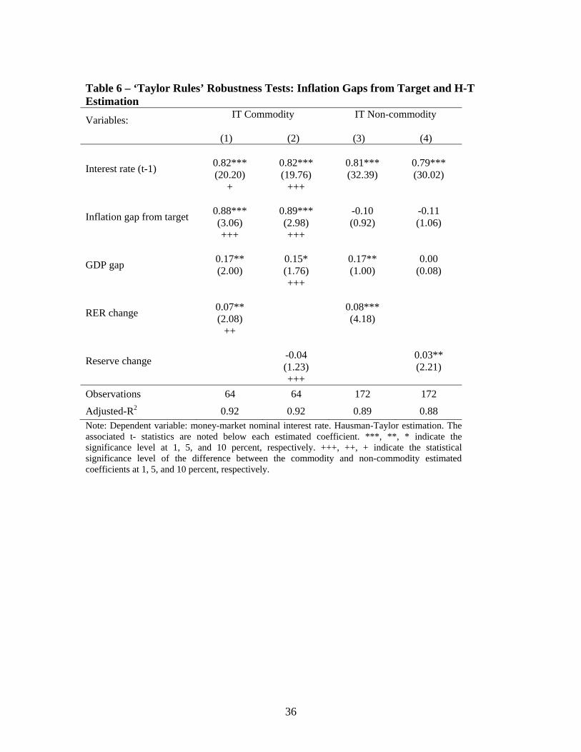
Columns (1) and (3) of Table 6 reports the results using the H-T estimation
procedure and using deviations from the time-varying inflation target for the IT
commodity and IT non-commodity countries. (These equations are analogous to Table 5).
Firstly, it is noteworthy that estimates for the inflation gap from target response in Table
6 for the IT commodity and IT non-commodity countries are larger than inflation
response reported in Table 5. The impact (long-term) response of inflation from target for
the commodity IT countries is to raise interest rates by about 0.88 (4.9) percentage points
in Table 6 and 0.88 (2.8) percentage points in Table 5. These estimates suggest
substantial short-run and long-run responses in nominal interest rates, and a substantial
long-run response in real interest rates, to an increase in inflation in the IT commodity-
intensive countries. Secondly, the output gap is highly significant in columns (1) and (3),
contrasting sharply with the results presented in Table 5. Thirdly, the real exchange rate
change variable coefficient is highly statistically significant and almost identical in
magnitude in columns (1) and (3). This differs from Table 5 where the estimated
response in the commodity IT countries is much larger in magnitude compared to non-
commodity IT countries.
Finally, we include changes in international reserves in the second and fourth
columns of Table 6. The change in international reserves is only significant in the non-
commodity IT countries, suggesting that a rise in reserves is associated with a rise in
interest rates.
(e) Are IT countries using the real exchange rates as an indicator of future inflation?
Our results suggest that external factors are important even for inflation targeting
policymakers. Central banks operating under inflation targeting regimes in emerging
22
markets react to current monetary conditions and current inflation as well as to changes in
real exchange rates. However, this observation does not necessarily imply that IT
policymakers have policy targets other than inflation, such as the setting of a specific real
exchange rate. It is possible that policymakers observe changes in current real exchange
rate as an indicator of future inflation and therefore react to it contemporaneously.26
In a previous draft, we included a section that estimates a reduced-form panel
VAR model (Aizenman et al., 2008). We failed to find any impact from real exchange
rate depreciation to higher future inflation. However, inflation does appear to lead to
future exchange rate changes in both the IT and non-IT samples. From these findings,
there is no evidence that real exchange rates are a good predictor of future inflation and
therefore should not in principle enter a forward-looking IT strategy policy equation if
inflation is the target for policymakers. The significant responses to real exchange rates in
the estimated policy equations, presented in Tables 2, 3, 5 and 6, appear to reflect a
separate policy target beyond an inflation target.
5. CONCLUSION
In this paper we explore the nature of inflation targeting in emerging market and
transition economies. In the context of an estimated panel data for 16 emerging markets
over 1989Q1 to 2006Q4 (using both IT and non-IT observations), we find clear evidence
of a significant and stable response running from inflation to policy interest rates in
emerging markets that are following publically announced IT policies. By contrast, we
find that non-IT central banks place much less weight on inflation in setting interest rates.
We emphasize that external considerations should play an important role in
central bank policy in emerging markets, and further identify countries that are more
23
vulnerable to terms-of-trade shocks as ones who respond more aggressively to
movements in the real exchange rates. Emerging markets generally have a low level of
financial market development, characterized by few instruments and thin trading, which
in turn are not able to play a significant role in stabilizing domestic output in the face of
external shocks (Aghion et al., 2006). To motivate our empirical findings, we present a
simple model that illustrates the linkages between external vulnerability and the role of
the real exchange rate in optimal policy rules.
We test whether emerging markets are following “pure” IT rules, or are also
attempting to stabilize real exchange rates. We find strong evidence that IT emerging
markets are following a mixed-IT strategy whereby central banks respond to both
inflation and real exchange rates in setting policy interest rates. The response to real
exchange rates is much stronger in non-IT countries, however, suggesting that
policymakers are more constrained in the IT regime—they are attempting to
simultaneously target both inflation and real exchange rates and these objectives are not
always consistent.
We also find that the response to real exchange rates is strongest in those
countries following IT policies that are relatively intensive in exporting basic
commodities. This is not surprising since this group is the most vulnerable to terms-of-
trade and real exchange rate disturbances. Moreover, the real exchange rate stabilization
objective does not appear to be influencing central bank interest rate-setting indirectly
because it is a good predictor of future inflation (as would be the case if inflation is a
good predictor and the central bank is forward looking), i.e. the real exchange rate is not
a robust predictor of future inflation in emerging markets. Consistent with our model’s

24
predictions, real exchange rate stabilization in commodity-intensive countries appears to
be related to adverse real output effects associated with real exchange rate volatility.

25
References
Aghion, P., Bacchetta, P., Ranciere, R., & Rogoff, K. (2009). Exchange rate volatility
and productivity growth: The role of financial development. Journal of Monetary
Economics, 56(4), 494-513.
Aizenman, J. (2008). International reserves management and the current account. In K.
Cowan, S. Edwards, S., & R. Valdés (eds.), Current Account and External Financing (pp.
435-474). Santiago: Central Bank of Chile.
Aizenman, J., Hutchison, M., & Noy, I. (2008). Inflation targeting and real exchange
rates in emerging markets. NBER Working Paper 14561.
Aizenman, J., & Riera-Crichton, D. (2008). Real exchange rate and international reserves
in the era of growing financial and trade integration. Review of Economics and Statistics,
90, 812-815.
Amato, J. D., & Gerlach, S. (2002). Inflation targeting in emerging market and transition
economies: Lessons after a decade. European Economic Review, 46(4-5), 781-790.
Arellano, M., & Bond, S. (1991). Some tests of specification for panel data: Monte Carlo
evidence and an application to employment equations. Review of Economic Studies, 58,
277-297.
Ball, C., & Reyes, J. (2004). Inflation Targeting or Fear of Floating in Disguise?
Mexico’s Post-Tequila Monetary Policy. International Journal of Finance and
Economics, 9(1), 49 – 69.
Ball, C., & Reyes, J. (2008). Inflation targeting or fear of floating in disguise? A broader
perspective. Journal of Macroeconomics, 30(1), 308 – 326.
Ball, L. (1998). Policy rules for open economies. NBER Working paper 6760.

26
Ball, L., & Sheridan, N. (2005). Does inflation targeting matter? In F. Mishkin & K.
Schmidt-Hebbel (eds.), Monetary Policy under inflation targeting, Santiago: Central
Bank of Chile.
Baltagi, B. H. (2005). Econometric analysis of panel data. West Sussex: Wiley & Sons; 2005.
Beck, T., & Demirgüç-Kunt, A. (2009). Financial institutions and markets across
countries and over time: data and analysis. World Bank Policy Research Working Paper
4943.
Breitung, J. (2000). The local power of some unit root tests for panel data. Advances in
Econometrics, 15, 161-178.
Brito, R. D., & Bystedt, B. (2010). Inflation targeting in emerging economies: Panel
evidence. Journal of Development Economics, 91, 198–210.
Calvo, G., & Reinhart, C. (2002). Fear of floating. Quarterly Journal of Economics,
107(2), 379-408.
Carare, A., & Stone, M. (2006). Inflation targeting regimes. European Economic Review,
50, 1297–1315.
Clarida, R. H. (2001). The Empirics of Monetary Policy Rules in Open Economies.
International Journal of Finance and Economics, 6, 315-323.
Clardia, R. H., Gali, J., & Gertler, M. (1998). Monetary policy rules in practice: some
international evidence. European Economic Review, 42, 1033-1067.
Clardia, R. H., Gali, J., & Gertler, M. (2000). Monetary policy rules and macroeconomic
stability: Evidence and some theory. Quarterly Journal of Economics, 115(1), 147-180.
27
Clardia, R. H., Gali, J., & Gertler, M. (2001). Optimal monetary policy in closed versus
open economies. American Economic Review, 91(2), 253–257.
Corbo, V., Landerretche, O., & Schmidt-Hebbel, K. (2001). Assessing inflation targeting
after a decade of world experience. International Journal of Finance and Economics, 6,
343-368.
De Mello, L. (2008). Monetary Policies and Inflation Targeting in Emerging Economies.
Paris: OECD.
De Mello, L., & Moccero, D. (2008). Monetary policy and macroeconomic stability in
Latin America: The cases of Brazil, Chile, Colombia and Mexico. In L. De Mello (ed.),
Monetary Policies and Inflation Targeting in Emerging Economies. Paris: OECD Press.
Dennis, R. (2003). Exploring the role of the real exchange rate in Australian monetary
policy. The Economic Record, 79(244), 20-38.
Dueker, M., & Fischer, A. (2006). Do inflation targeters outperform non-targeters?
Federal Reserve Bank of St. Louis Review, 3, 431-450.
Edwards, S. (2006). The relationship between exchange rates and inflation targeters
revisited. NBER Working Paper 12163.
Eichengreen, B. (2007). Comment on Cheung, Chinn and Fujii: The overvaluation of
Renminbi undervaluation. Journal of International Money and Finance, 26(5), 657-864.
Enders, W. (2003). Applied Econometric Time Series. West Sussex: Wiley and Sons.
English, N., & Sack, X. (2002). Interpreting the significance of the lagged interest rate in
estimated monetary policy rules. Working paper, Division of Monetary Affairs, Board of
Governors of the Federal Reserve System.
28
Fraga, A., Goldjfan, I., & Minella, A. (2003). Inflation Targeting in Emerging Market
Economies. NBER Macroeconomics Annual.
Gonçalves, C. E. S., & Salles, J. M. (2008). Inflation targeting in emerging economies:
What do the data say? Journal of Development Economics, 85, 312-318.
Greene, W., 2007. LIMDEP Econometric Modeling Guide Vol. 1. New York:
Econometric Software, Inc.
Hausman J, & Taylor W. (1981). Panel data and unobservable individual effects.
Econometrica, 49(6), 1377-1398.
International Monetary Fund (2005). World Economic Outlook. Washington, D.C.: IMF
Press.
Johnson, D. (2002). The effect of inflation targeting on the behavior of expected
inflation: evidence from an 11 country panel. Journal of Monetary Economics, 49, 1521-
1538.
Judson, R.A., & Owen A.L. (1999). Estimating dynamic panel models: a guide for
macroeconomists. Economics Letters, 65, 9-15.
Kézdi, G. (2004). Robust standard error estimation in fixed-effects panel models.
Hungarian Statistical Review, 9, 95-116.
Levin, A., Lin, C. F., & Chu, C. S. (2002). Unit root tests in panel data: asymptotic and
finite-sample properties. Journal of Econometrics, 108(1), 1-24.
Lin S., & Ye, H. (2009). Does inflation targeting make a difference in developing
countries? Journal of Development Economics, 89, 118–123.
Miao, Y. (2009). In search of successful inflation targeting: evidence from an inflation
targeting index. IMF Working Paper 09/148.
29
Mishkin, F. S. (2004). Can inflation targeting work in emerging markets? NBER
Working Paper 10646.
Mishkin, F. S., & Schmidt-Hebbel, K. (2007). Does inflation targeting make a
difference? NBER Working Paper 12876.
Mohanty, M.S., & Klau, M. (2004). Monetary policy reules in emerging market
economies: issues and evidence. BIS Working Paper 149.
Nickell, S. (1981). Bias in panel models with fixed effects. Econometrica, 49, 1417-1426.
Park, Y. C. (2009). Reform of the global regulatory system: Perspectives of East Asia’s
emerging economies. ABCDE World Bank Conference Proceedings.
Pavasuthipaisit, R. (2010). Should inflation-targeting central banks respond to exchange
rate movements? Journal of International Money and Finance, 29, 460–485
Petersen, M. A. (2009). Estimating standard errors in finance panel data sets: comparing
approaches. Review of Financial Studies, 22(1), 435-480.
Ravenna, F. (2008). The impact of inflation `targeting: testing the good luck hypothesis.
Mimeo. University of California, Santa Cruz, Department of Economics.
Reyes, J. (2007). Exchange rate pass-through effect and inflation targeting in emerging
economies: what is the relationship? Review of International Economics, 15(3), 538 -
559.
Rose, A. (2007). A stable international monetary system emerges: Inflation targeting is
Bretton Woods, reversed. Journal of International Money and Finance, 26, 663-681.
Schmidt-Hebbel, K., & Werner, A. (2002). Inflation targeting in Brazil, Chile and
Mexico: Performance, credibility, and the exchange rate. Economía, 2, 31-89.

30
Taylor, J. B., (2001). The role of the exchange rate in monetary policy rules. American
Economic Review, 91, 263–267.
Wollmershäuser, T. (2006). Should central banks react to exchange rate movements? An
analysis of the robustness of simple policy rules under exchange rate uncertainty. Journal
of Macroeconomics, 28, 493–519.

31
Table 1 – Descriptive Statistics for Macroeconomic Variables
Variable:
IT Sample
(456 obs.)
Non-IT Sample
(577 obs.)
t-stat for difference
between samples
GDP growth (%) 1.11
(5.93) 1.00
(7.84) 0.26
GDP gap (%)
-0.11 (3.86)
0.29 (4.62)
1.52
Inflation (%)
5.40 (4.21)
9.60 (9.15)
9.79***
Interest rate (%)
8.98 (6.09)
12.68 (10.25)
7.21***
Real exchange rate change (%)
2.50 (5.76)
-0.49
(13.27) 4.86***
Foreign reserve change (%)
3.25 (7.89)
4.66
(22.82) 1.38
Mean and (standard deviation) for all variables. ***, **, * indicate the significance level at 1, 5, and 10 percent, respectively.
32
Table 2 – ‘Taylor Rules’: Baseline Model
IT Non IT
Variable (1) (2) (3) (4) (5) (6)
Interest rate (t-1)
0.84*** (43.97)
+++
0.83*** (43.36)
+++
0.84*** (43.91)
+++
0.76*** (22.50)
0.74*** (22.48)
0.77*** (23.17)
Inflation
0.22* (1.86) +++
0.29** (2.43) +++
0.22* (1.86) +++
0.01 (0.72)
0.15*** (5.08)
0.01 (0.62)
GDP gap
0.03
(1.05) ++
0.05 (1.55) +++
0.03 (1.05) +++
0.02 (0.37)
0.03 (0.62)
0.02 (0.52)
RER change
0.07*** (3.46) +++
0.13*** (5.78)
Reserve change
0.09
(0.05)
-0.06*** (-3.95)
Observations 387 387 387 472 472 472
Adjusted-R2 0.76 0.77 0.76 0.79 0.80 0.73 F-test 272.10 206.89 203.60 177.55 151.01 141.35 Note: Dependent variable: money-market nominal interest rates. Panel fixed-effects estimation. The associated t- statistics are noted below each estimated coefficient. ***, **, * indicate the significance level at 1, 5, and 10 percent, respectively. +++, ++, + indicate the statistical significance level of the difference between the IT and non-IT estimated coefficients at 1, 5, and 10 percent, respectively.
33
Table 3 – Commodity Intensities Country Commodities as percent of total exports
1997 2006Argentina 36.63% 35.98%Brazil* 26.74% 31.26%Colombia* 54.62% 54.26%Czech Republic* 20.52% 16.85%Hungary* 16.13% 11.81%Indonesia 37.80% 41.90%Israel* 8.22% 6.70%Jordan 10.49% 12.56%Korea* 13.19% 17.16%Malaysia 15.70% 20.48%Mexico* 20.00% 22.84%Morocco 20.10% 16.45%Peru* 31.93% 32.26%Philippines* 4.95% 9.92%Poland* 24.57% 21.97%Thailand* 13.89% 15.55%* IT‐sample countries. Source: United Nations Commodity Trade Statistics Database (UN Comtrade) and National Accounts Main Aggregates Database, United Nations Statistics Division. We define commodities as HS codes 1‐10, 27‐29, 44, 47‐48, 72‐76 and 78‐81. In bold are the countries we define as commodity‐intensive exporters.
34
Table 4 – Descriptive statistics: Commodity and Non-Commodity IT groups
Variable
IT Commodity
(88 obs.)
IT Non-Commodity
(200 obs.)
t-stat for difference between samples
GDP gap (%)
-0.22 (3.35)
-0.25 (4.24)
0.06
Inflation (%)
1.75
(1.10)
0.66
(0.92) 8.13***
Interest rate (%)
12.87 (7.43)
8.30
(5.46) 5.19***
Real exchange rate change (%)
4.04
(7.58)
3.06
(5.52) 1.09
Means for each variable/sample. Standard errors are denotes in (). ***, **, * indicate the significance level at 1, 5, and 10 percent, respectively..
35
Table 5 – ‘Taylor Rules’: Commodity-intensive and Non-commodity intensive groups (with robust standard errors)
IT Commodity IT Non-commodity
Interest rate (t-1)
0.69 (11.39)*** [7.23]*** {4.43}***
+++
0.88 (50.24)*** [27.98]*** {9.14}***
Inflation
0.92
(2.12)** [1.66]* {1.13}
+++
0.10
(0.87) [0.62] {0.25}
GDP gap
0.09
(0.71) [1.21] {0.72}
+++
0.04
(3.92)*** [3.84]***
{0.20}
RER change
0.13
(1.98)** [1.71]* {1.76}*
+++
0.08
(1.55) [1.19] {0.13}
Observations 88 200
Adjusted-R2 0.66 0.93 F-test 44.15 661.22 Note: Dependent variable: money-market interest rates. The associated t- statistics are noted below each estimated coefficient. () denotes unadjusted standard errors, [] denotes clustered standard errors, and {} denotes Newey-West standard errors. For the exact algorithms for calculating the standard errors, please see Greene (2008, pp. R16 31-33). ***, **, * indicate the significance level at 1, 5, and 10 percent, respectively for the rejection of the null of no effect. +++, ++, + indicate the statistical significance level of the difference between the commodity and non-commodity estimated coefficients with the clustered standard errors at 1, 5, and 10 percent, respectively.
36
Table 6 – ‘Taylor Rules’ Robustness Tests: Inflation Gaps from Target and H-T Estimation Variables:
IT Commodity
(1) (2)
IT Non-commodity
(3) (4)
Interest rate (t-1)
0.82*** (20.20)
+
0.82*** (19.76)
+++
0.81*** (32.39)
0.79*** (30.02)
Inflation gap from target
0.88*** (3.06) +++
0.89*** (2.98) +++
-0.10 (0.92)
-0.11 (1.06)
GDP gap
0.17** (2.00)
0.15* (1.76) +++
0.17** (1.00)
0.00
(0.08)
RER change
0.07** (2.08)
++
0.08*** (4.18)
Reserve change
-0.04 (1.23) +++
0.03** (2.21)
Observations 64 64 172 172
Adjusted-R2 0.92 0.92 0.89 0.88 Note: Dependent variable: money-market nominal interest rate. Hausman-Taylor estimation. The associated t- statistics are noted below each estimated coefficient. ***, **, * indicate the significance level at 1, 5, and 10 percent, respectively. +++, ++, + indicate the statistical significance level of the difference between the commodity and non-commodity estimated coefficients at 1, 5, and 10 percent, respectively.

37
Appendix A: Inflation targeting in the open economy: economic structure and the real exchange rate. This Appendix illustrates conditions that may lead the policy maker to adopt IT rule that
would include exchange rate in the policy rule. We focus on the simplest set up that
illustrates this point. A well know benchmark paper is Ball (1998), studying inflation
targeting in the open economy, where setting the interest rate and the exchange rate
impacts future output and inflation. Assuming that the inflation target and potential
output (π% and y% , respectively) are exogenously given, the IT rule is designed to
minimize the loss function [equivalently, minimizing ( ) ( )L V V y yπ π μ= − + −% % ]:
( ) ( )L V V yπ μ= + (A1)
where y is the log of real output (measured as deviations from average levels), π is
inflation,μ is the relative weighted attached to output versus inflation objectives, and
V(x) is the variance of x. In Ball’s set up, the exchange rate (e) plays a role in the IT
setting if it affects inflation or output, leading to the conclusion that “…if the authorities
have modeled the economy correctly (and, in doing so, have incorporated the effects of e
on π and y), there is no need to include an exchange rate term in (the IT) equation” (see
Edwards, 2006). Edwards (2006) also notes that “If, however, there is a lagged response
of inflation and output to exchange rate changes, the central bank may want to preempt
their effect by adjusting the policy stance when the exchange rate change occurs, rather
than when its effects on π and y are manifested.”27
In this Appendix we show that the role of the exchange rate and economic
structure is more involved in circumstances where potential output is affected by
exchange rate volatility.28 To illustrate this point, suppose that potential output, y% ,
depends negatively on exchange rate volatility, ( ( )); ' 0y y V e y= <% % % . The modified loss
function facing the policy maker would be
( ) ( ) ( )L V V y V eπ μ φ= + +)
(A2)
where φ reflects the welfare cost associated with the drop in potential output induced by
exchange rate volatility. To simplify the discussion, we modify Ball’s model into a set

38
up where the adjustment to shocks happens within the period, without persistence.29
Applying Ball’s notation, the base system we consider is:
.
.
.
a y r eb y ec e r
β δ επ α γ η
θ υ
= − − += − += +
(A3)
where all parameters are positive, all variables are measured as deviations from average
levels, y is the deviation of output from the trend “potential output,” r is the real interest
rate, e is the real exchange rate (a higher e means appreciation), π is inflation, and ε , η ,
and v are white-noise shocks. Equation (A3a) is an open-economy IS curve. Output
depends on lags of the real interest rate and the real exchange rate, and a demand shock.
Equation (A3b) is an open-economy Phillips curve. The change in inflation depends on
output’s deviations from “potential output”, the exchange rate, and a shock. The change
in the exchange rate affects inflation because it is passed directly into import prices.
Equation (A3c) links the interest rate and the exchange rate, assuming that a rise in the
interest rate makes domestic assets more attractive, leading to an appreciation. The shock
v reflects other considerations impacting the exchange rate (investor confidence, foreign
interest rates, risk premium, etc).
Suppose that the central bank chooses the real interest rate r applying a modified
inflation targeting rule:
r a by ceπ= + + (A4)
Applying (A4) to (A3), we solve for the implied inflation, output and the exchange rate
volatility as a function of the shocks and the IT parameters <a, b, c>. It can be shown
that 2 2 2 2
2 2 2
2 2 2
. ( ) ( ) ( ) [1 ( )] ( ) ( ) ( ) /
. ( ) (1 ( )) ( ) [ ( ) ] ( ) ( ) ( ) /
. ( ) ( (1 ) ) ( ) [ ( ) ] ( ) (1 ) ( ) /
a V e b a V b a V a V D
b V y a c V a c V aB V D
c V c b V c b V c bB V D
α θ ε β α υ θ μ
θ α ε β α δ υ μ
π α θ γθ ε β α γ δα γ υ θ μ
⎡ ⎤= + + + + +⎣ ⎦⎡ ⎤= + − + − − +⎣ ⎦⎡ ⎤= − − + + + + + − +⎣ ⎦
(A5) ,
where 2[1 ( ) ( )]D B b a a cα θ α= + + + − , B β δθ= + .
Feeding (A5) to the loss function (A2), the optimal IT rule is inferred by minimizing the
loss resultant function [i.e., the <a, b, c> that minimize the loss function (A2)].
Note that (A5a) implies that a negative weight on the exchange rate parameter (c < 0)
tends to reduce exchange rate volatility. This will be the with a policy rule where
39
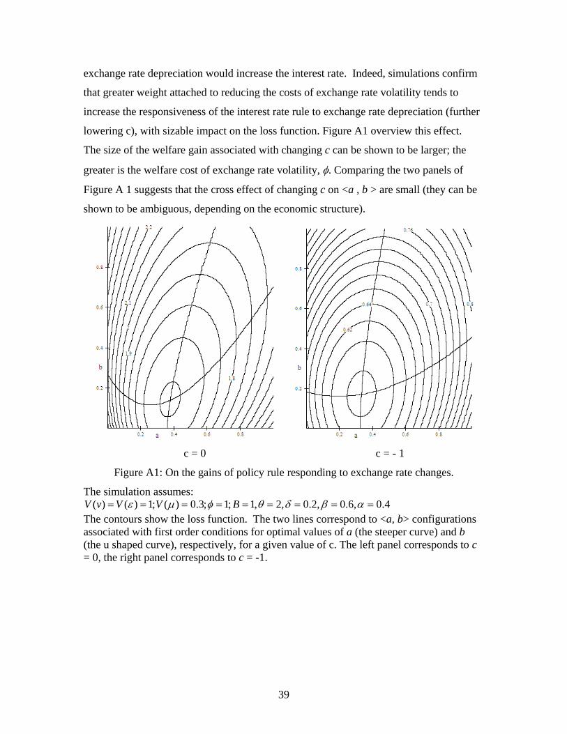
exchange rate depreciation would increase the interest rate. Indeed, simulations confirm
that greater weight attached to reducing the costs of exchange rate volatility tends to
increase the responsiveness of the interest rate rule to exchange rate depreciation (further
lowering c), with sizable impact on the loss function. Figure A1 overview this effect.
The size of the welfare gain associated with changing c can be shown to be larger; the
greater is the welfare cost of exchange rate volatility, φ. Comparing the two panels of
Figure A 1 suggests that the cross effect of changing c on <a , b > are small (they can be
shown to be ambiguous, depending on the economic structure).
c = 0 c = - 1
Figure A1: On the gains of policy rule responding to exchange rate changes.
The simulation assumes: ( ) ( ) 1; ( ) 0.3; 1; 1, 2, 0.2, 0.6, 0.4V v V V Bε μ φ θ δ β α= = = = = = = = =
The contours show the loss function. The two lines correspond to <a, b> configurations associated with first order conditions for optimal values of a (the steeper curve) and b (the u shaped curve), respectively, for a given value of c. The left panel corresponds to c = 0, the right panel corresponds to c = -1.
40
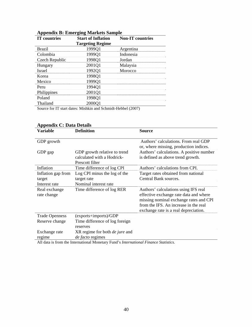
Appendix B: Emerging Markets Sample IT countries
Start of Inflation Targeting Regime
Non-IT countries
Brazil 1999Q1 Argentina Colombia 1999Q1 Indonesia Czech Republic 1998Q1 Jordan Hungary 2001Q1 Malaysia Israel 1992Q1 Morocco Korea 1998Q1 Mexico 1999Q1 Peru 1994Q1 Philippines 2001Q1 Poland 1998Q1 Thailand 2000Q1 Source for IT start dates: Mishkin and Schmidt-Hebbel (2007) Appendix C: Data Details Variable
Definition Source
GDP growth Authors’ calculations. From real GDP or, where missing, production indices.
GDP gap GDP growth relative to trend calculated with a Hodrick-Prescott filter
Authors’ calculations. A positive number is defined as above trend growth.
Inflation Time difference of log CPI Authors’ calculations from CPI. Inflation gap from target
Log CPI minus the log of the target rate
Target rates obtained from national Central Bank sources.
Interest rate Nominal interest rate Real exchange rate change
Time difference of log RER Authors’ calculations using IFS real effective exchange rate data and where missing nominal exchange rates and CPI from the IFS. An increase in the real exchange rate is a real depreciation.
Trade Openness (exports+imports)/GDP Reserve change Time difference of log foreign
reserves
Exchange rate regime
XR regime for both de jure and de facto regimes
All data is from the International Monetary Fund’s International Finance Statistics.

41
Appendix D: Unit Root Tests
IT Non-IT
LLC Breitung LLC Breitung
GDP gap 6.69 -3.45** 2.37 -3.37**
Inflation -9.09** -1.56* 3.50 -3.00**
Interest rate -12.29** 0.58 -2.46** -0.72
Real exchange rate change
-11.77** -7.88** -12.66** -1.21
Note: The results are based on Levin, Lin and Chu (2002) and Breitung (2000) tests. **, * indicates the rejection of the common unit root null hypothesis at 5% and 10% significance level, respectively. As is true for all other panel unit root tests, these tests should be interpreted with caution since both tests assume a common process. Any deviation from that assumption will entail a rejection of the null, even if some country time-series do have a unit root. Individual country unit root tests will have weak power with quarterly data. For a summary of the difficulties with panel unit root tests, see Enders (2003, chapter 4.11).
Appendix E: Descriptive Statistics for TOT Variable Variable IT Non-IT
Terms of Trade change (%) (IMF data)
0.04 (1.65) [456]
-0.09 (1.18) [585]
Terms of Trade change (%) (IFS data)
0.34 (4.11) [268]
0.07 (7.88) [354]
Terms of Trade change (%) (Datastream data)
0.34 (4.10) [299]
0.57 (5.88) [191]
Correlations of TOT Variables TOT(IMF)-TOT(IFS): 0.03 TOT(IMF)-TOT(DS): 0.08 TOT(DS)-TOT(IFS): 0.13 Mean, (standard error), [observations]. For details, see the data appendix.
42
1 Fourteen of the 30 OECD countries have explicit inflation targets. However, twelve of the countries
without an explicit target are in the EMU and operate under a single central bank (ECB). Hence, fourteen
of the 19 “operational” central banks in the OECD target inflation.
2 This debate has recently subsided as a result of the global financial crisis. It will surely re-emerge once the
anticipated recovery takes hold and inflation fears will resurface again
3 Some exceptions are IMF (2005), Conçalves and Salles (2008), Schmidt-Hebbel (2002), Mishkin and
Schmidt-Hebbel (2007), Corbo et al. (2001) and Edwards (2006) in empirical work and Reyes (2007) in
theoretical modeling.
4 Thirteen advanced industrial countries that “…are at the international frontier of macro-economic
management and performance.” (p. 4)
5The authors do not consider a control group of emerging countries that are not targeting inflation.
6 Carare and Stone (2006) is an earlier contribution that also empirically examines the range of inflation
targeting possibilities.
7 One drawback of these time-series regressions is the very short sample periods. The authors use monthly
data for Brazil and Mexico, and quarterly data for Chile.
8 They estimate one equation for each country over the 1990s. Hence, in most cases, their estimated
coefficients average periods of both inflation-targeting and non-targeting for countries that eventually
adopted an IT regime.
9 The specification of the model shares the characteristics of the benchmark literature. Even though the real
exchange rate is beyond the control of the policy maker in the long-run, in the short and intermediate-runs a
significant share of the GDP is transacted at pre-set prices. Consequently, in the short-run, nominal
exchange rate changes impact the real exchange rate. This is evident in the higher short run correlations
between the nominal and the real exchange rate than the one observed in the intermediate and long-runs.
10 They found that the adverse effects of exchange rate volatility become insignificant for countries at the
financial development level of Euro area, the U.K., Switzerland, Finland, Sweden, the US, and Australia.

43
11 For example, Korea’s ratio of private credit to GDP was 101% in 2007 – by far the highest in our
emerging market sample, and not very different from most other OECD members (data from Beck and
Demirgüç-Kunt, 2009). However, during the recent crisis, Korea appeared very vulnerable to exchange rate
volatility (Korea’s experience during the crisis is overviewed in Park, 2009).
12 A growing literature has identified financial intermediation, in the presence of collateral constraints, as a
mechanism explaining the hazard associated with credit cycles induces by shocks. The prominent role of
bank financing in developing countries suggests that balance sheet valuation problems associated with
shocks may lead to higher cost of borrowing, reducing average growth, and possibly to recessions in the
aftermath of adverse shocks. In these circumstances, real exchange rate changed induced by adverse terms
of trade shocks or contagion may impose adverse liquidity shocks, propagating lower output growth. This
channel is of greater potency in countries where most financial intermediation is done by banks, relying on
debt contracts. Less efficient judiciary, higher monitoring and enforcement costs tend to magnify the
adverse impact of real exchange shocks on the costs of credit; for further references and models of the
credit channel in developing countries see Aghion et al. (2006) and Aizenman (2008).
13 Another possible motivation for the policymaker’s decision to respond to the exchange rate may be
related to the fear-of-floating findings reported by Calvo and Reinhart (2002) and the pass-through from
exchange rates to domestic inflation.
14 Aizenman and Riera-Crichton (2008) argue that an IT rule responding to the exchange rate may be
supplemented by a corresponding international reserve policy. Our empirical specification also considers
this possibility by controlling for changes of international reserves.
15 Chile was excluded from the data set because the country’s policy functions appear anomalous to the
other IT countries in the sample. Corbo et al. (2001) estimate Taylor rules for 25 countries and only in the
case of Chile do they estimate a real interest rate equation. We similarly find Chile to be an outlier in our
panel-data Taylor rule regressions, even when including fixed effects in the estimation procedure.
16 As documented by Enders (2003) and others, panel unit root tests are quite sensitive to a number of data
characteristics and are difficult to interpret.
17 It is well known that the LSDV estimation with a lagged dependent variable is biased when the time
dimension of the panel (T) is small. Nickell (1981) shows that this bias approaches zero as T approaches
44
infinitely. Judson and Owen (1999), in a Monte Carlo study, shows that the LSDV estimator performs well
in comparison with GMM and other estimators when T=30. In an unbalanced panel with T=30, LSDV
performs best. T is equal to 68 on our study and the bias is presumably small.
18 For robustness, we also estimated the benchmark regressions using the Clarida (2001) specification that
includes both contemporaneous and lagged inflation as independent variables. Results on the magnitude of
the effect of inflation on the interest rate are practically the same.
19 In results not reported, we also included a trade openness measure (exports plus imports as % of GDP).
We find that the interest rate response to real exchange rates of the IT group does not appear to be affected
by the degree of trade openness and the estimated coefficients on the other variables are nearly identical to
the specifications reported in Table 2.
20 In preliminary work, we also considered policy rules with terms-of-trade shocks entered explicitly into
the estimation equation. The difficultly was in obtaining an accurate terms-of-trade measure. We
considered three measures of terms-of-trade: From the International Monetary Fund’s International Finance
Statistics, from Datastream, and a TOT measure used by International Monetary Fund staff internally for
the calculations presented in the World Economic Outlook. These measures were not significantly
correlated with each other, despite purporting to measure the same phenomenon. None of these measures
were statistically significant when included in the interest rate policy equations. We have little confidence
in the reliability of these terms-of-trade measures, although all are derived from official sources, and do not
report statistical results where they are included.
21 The basic Taylor equation model is estimated with the addition of real exchange rates in Table 5 for IT
countries, separating the sample into commodity-intensive and non-intensive countries. Reserve changes
for the IT countries were not significant in Table 3 or Table 5, and are not reported for brevity.
22 All inflation data are annualized quarterly rates.
23 In Monte Carlo studies Kézdi (2004) and Petersen (2009) conduct, they both find the bias associated with
estimations of the fixed effect model with clustered standard errors to be small in finite samples.
24 The data on the explicit inflation target, for each central bank, was collected from the central bank’s
country-specific publications.
45
25 Identification in the Hausman-Taylor procedure requires that the number of exogenous variables be at
least as large as the number of time-invariant predetermined/endogenous variables.
26 Clarida (2001) discusses this issue in the context of a forward-looking IT regime.
27 Taylor (2001) and Wollmershäuser (2006) are also relevant models.
28 Aghion et al. (2006) showed that exchange rate volatility reduces potential output (or output growth rate)
in developing countries, attributing it to financial channels. The adverse effect of volatility may be the
outcome of increasing the expected cost of funds in circumstances where agency and contract enforcement
costs are prevalent, the financial system is shallow, and trade openness is significant.
29 This may be the case if all the nominal contracts are re-set at the end of each period.