inferring tennis match progress from in-play betting · pdf fileinferring tennis match...
TRANSCRIPT

Inferring Tennis Match Progress from In-Play
Betting Odds : Project Report
James Wozniak4th year Information Systems Engineering MEng
Supervised by Dr. William Knottenbelt
June 23, 2011
1

Abstract
This project examines the way in which tennis matches are modelled to ob-tain the probabilities of a each player winning a match in progress. By takinglive market data from the betting website Betfair, the live odds are analysed andcompared against those generated from the derived tennis model. Based on thiscomparison, an algorithm is described to infer the scoreline of the match fromthe Betfair data. This algorithm is then improved by detecting breaks in play,and using them to correct any errors in the score prediction.
2

Acknowledgements
I would like to thank Dr. William Knottenbelt for providing the idea behind theproject and for providing valuable insight, guidance and motivation. I wouldalso like to thank Professor Peter Harrison for his suggestions and help in re-viewing the progress of the project. Lastly, I would like to thank my parentsfor their financial and morale support throughout my education.
3

Contents
1 Introduction 6
2 Background 62.1 Tennis Scoring System[2] . . . . . . . . . . . . . . . . . . . . . . . 6
2.1.1 Service . . . . . . . . . . . . . . . . . . . . . . . . . . . . . 62.1.2 Games . . . . . . . . . . . . . . . . . . . . . . . . . . . . . 72.1.3 Sets . . . . . . . . . . . . . . . . . . . . . . . . . . . . . . 72.1.4 Tie-breaks . . . . . . . . . . . . . . . . . . . . . . . . . . . 7
2.2 Betting odds . . . . . . . . . . . . . . . . . . . . . . . . . . . . . 72.2.1 Sources . . . . . . . . . . . . . . . . . . . . . . . . . . . . 8
2.3 Statistical Modeling . . . . . . . . . . . . . . . . . . . . . . . . . 92.3.1 Stochastic Markov chains . . . . . . . . . . . . . . . . . . 9
2.4 Tennis formulas . . . . . . . . . . . . . . . . . . . . . . . . . . . . 102.4.1 Game formula . . . . . . . . . . . . . . . . . . . . . . . . 102.4.2 Set and tie-breaker formula . . . . . . . . . . . . . . . . . 112.4.3 Match formula . . . . . . . . . . . . . . . . . . . . . . . . 12
2.5 Independence of points . . . . . . . . . . . . . . . . . . . . . . . . 13
3 Obtaining in-play betting odds 133.1 Getting data from Betfair . . . . . . . . . . . . . . . . . . . . . . 143.2 Information Available . . . . . . . . . . . . . . . . . . . . . . . . 14
3.2.1 Virtual bets and cross matching . . . . . . . . . . . . . . 143.3 Odds logging . . . . . . . . . . . . . . . . . . . . . . . . . . . . . 153.4 Projected Odds . . . . . . . . . . . . . . . . . . . . . . . . . . . . 16
4 Tennis Model 164.1 Inputs to the model . . . . . . . . . . . . . . . . . . . . . . . . . 164.2 Game formula . . . . . . . . . . . . . . . . . . . . . . . . . . . . . 174.3 Set formula . . . . . . . . . . . . . . . . . . . . . . . . . . . . . . 184.4 Match formula . . . . . . . . . . . . . . . . . . . . . . . . . . . . 204.5 Service faults . . . . . . . . . . . . . . . . . . . . . . . . . . . . . 214.6 Implementation of the Model . . . . . . . . . . . . . . . . . . . . 224.7 Simulator . . . . . . . . . . . . . . . . . . . . . . . . . . . . . . . 224.8 The importance of a point . . . . . . . . . . . . . . . . . . . . . . 24
5 Comparison between Model and Live Odds 255.1 Schiavone V Li . . . . . . . . . . . . . . . . . . . . . . . . . . . . 255.2 Schiavone V Bartoli . . . . . . . . . . . . . . . . . . . . . . . . . 285.3 Murray V Nadal . . . . . . . . . . . . . . . . . . . . . . . . . . . 305.4 Determining PWOS probabilities from ‘in-play’ odds . . . . . . . 32
6 Inferring the score 34
4

7 Non-corrective bounds checking 347.1 Method . . . . . . . . . . . . . . . . . . . . . . . . . . . . . . . . 347.2 Dealing with non-iid points . . . . . . . . . . . . . . . . . . . . . 357.3 Odds information . . . . . . . . . . . . . . . . . . . . . . . . . . . 367.4 Results . . . . . . . . . . . . . . . . . . . . . . . . . . . . . . . . . 37
7.4.1 Bartoli V Schiavone . . . . . . . . . . . . . . . . . . . . . 377.4.2 Schiavone V Li . . . . . . . . . . . . . . . . . . . . . . . . 397.4.3 Murray V Nadal . . . . . . . . . . . . . . . . . . . . . . . 407.4.4 Total amount matched . . . . . . . . . . . . . . . . . . . . 41
7.5 Conclusions . . . . . . . . . . . . . . . . . . . . . . . . . . . . . . 42
8 Error correction - Breaks in play 438.1 Rests . . . . . . . . . . . . . . . . . . . . . . . . . . . . . . . . . . 438.2 Explanation . . . . . . . . . . . . . . . . . . . . . . . . . . . . . . 438.3 Results . . . . . . . . . . . . . . . . . . . . . . . . . . . . . . . . . 45
8.3.1 Schiavone V Li . . . . . . . . . . . . . . . . . . . . . . . . 458.3.2 Bartoli V Schiavone . . . . . . . . . . . . . . . . . . . . . 498.3.3 Murray V Nadal . . . . . . . . . . . . . . . . . . . . . . . 52
8.4 Conclusions . . . . . . . . . . . . . . . . . . . . . . . . . . . . . . 528.4.1 Set Markets . . . . . . . . . . . . . . . . . . . . . . . . . . 52
9 Evaluation 53
10 Conclusion 54
11 Future Work 5511.1 Gambling Tool . . . . . . . . . . . . . . . . . . . . . . . . . . . . 5511.2 Further Error Correction . . . . . . . . . . . . . . . . . . . . . . . 56
5

1 Introduction
Over the last few years, the growth and widespread use of the Internet hashelped revolutionise the betting industry. The Internet offers a more efficientand convenient way to wager money, as well as opening the door for large scalebetting exchanges and ‘in-play’ markets. As a result, large volumes of moneyare now wagered continuously throughout the duration of many sporting events.
Analysing the betting exchange ‘Betfair’, a significant singles match of pro-fessional tennis can often see several millions of pounds traded between users[1].One match analysed in this report from the 2011 French Open Final, saw over25 million pounds traded. With the large volume of bets being placed, thisproject primarily aims to investigate how sensitive and adaptive the market isto the current progress of a tennis match. The overall goal is to see if the bettingmarket has grown to the point whereby the score of a match can be inferredfrom the odds offered on a particular exchange.
In order to relate the fluctuations in the live betting odds to the progress ofa tennis match, a mathematical model is developed under the assumption thateach point played is independent and identically distributed (iid). The modelprovides a way of calculating the probability of a player winning the matchfrom any possible scoreline based on a measure of the players relative skill level.Also discussed how is the ‘in-play’ odds are collected and what information isavailable for analysis.
The main investigation of the project is then performed with the aid of thetools created. The odds extracted from Betfair are compared against those gen-erated by the model for three different matches. Based on these observationsseveral methods are suggested to try and infer the score. These methods aredescribed, tested and evaluated, giving reasons for any successes or failures.
2 Background
2.1 Tennis Scoring System[2]
Tennis has a rather unusual and complicated scoring system and the exactscoring rules vary between different competitions and with the gender of theplayers. The basic system consists of a hierarchical model, with points requiredto win games, games required to win sets, and sets required to win the match.
2.1.1 Service
A player is allowed a single fault per point when on service. Performing twofaults on the same point forfeits the point. If a player loses the game on hisservice, then it is referred to as a ’break’. This is considered to be a significantevent due to the advantage of having service.
6
2.1.2 Games
Scoring within a game goes incrementally from 0, 15, 30, 40 and then game. Ifboth players reach 40 it is referred to as ‘deuce’. From deuce, winning a pointgives a player ‘advantage’. Winning a point with the ‘advantage’ wins the game,whilst losing with ‘advantage’ returns the game to deuce. The server remainsconstant throughout any given game and alternates between games. The serverof the first game of the match is determined by a coin toss.
2.1.3 Sets
The winner of the set is based upon the total number of games won by eachplayer during the set. Generally speaking, the set is won if a player has won sixor more games, and is at least two games clear of his opponent. If both playersreach six games all, then a tie-break occurs to determine the winner of the set.If both players can win the match by winning the current set, then it is knownas the final set.
In accordance to the rules of the particular tournament or competition, pro-fessional tennis matches are played either as the best of three sets (first playerto win two sets) or the best of five (first player to win three sets). There arealso varying rules about the final set, and whether or not the match can enter atiebreaker. In the case where there is no final set tiebreaker (common in majortournaments), the final set will continue past 6-6 as normal until a two gameadvantage is achieved.
2.1.4 Tie-breaks
A tie-breaker requires a player to score seven or more points, and have a twopoint lead against the opponent. For example, a tie-break can be won by 7-5,7-2 or 9-7. The winner of the tie-break determines the winner of the set by ascore of seven games to six. Service is rotated between both players. The playerwho served the first game of the set is given service for the first point. Thenext two points are served by the other player, and service is swapped everytwo points until a winner emerges.
2.2 Betting odds
The odds for a particular event or outcome are formulated as a ratio of twointegers, usually written as
n/m
where n and m represent the relative chance of the outcome not occurring andoccurring respectively. A bet of m currency units will then give a profit of nunits if successful. For example, the odds of getting a six on a dice roll are 5/1and if £10 is staked, the profit will be £50.
7

It is also common for betting exchanges, such as Betfair, to use a decimal rep-resentation of odds. Given the probability of an event occurring, p, the decimalodds are calculated as follows
Decimal odds =1
p
For example, if the probability of an outcome is 0.25, then the decimal odds willbe 4. Given this figure, it is easy to calculate the return of the bet
return = units staked ∗ decimal odds
The profit can be determined by subtracting the stake itself from the returns,i.e. by subtracting 1 from the decimal odds and multiplying. In this case, youwould win 3 times the stake if successful.
2.2.1 Sources
Traditional bookmakers are a source of up to date and ‘in-play’ betting odds.However, they do not offer what can be termed, ‘actual’ odds. That is, theirodds are not representative of the true probability of a certain outcome. Al-though arguably the probability of a certain outcome is subjective and can neverbe defined, they will deliberately try and offer slightly worse odds than what isbeing predicted to statistically ensure a profit. Without knowing or estimatingtheir desired profit margins, these odds are of little use.
Fortunately, as mentioned in the introduction, the amount of people gamblingon-line has allowed betting exchanges to grow rapidly in popularity. A bet-ting exchange allows users to place bets amongst each other, with users ableto assume the role of a bookmaker. As the exchange odds are decided by theusers, we can assume that they more closely represent the ’actual’ odds and thegeneral consensus of the user base as to a particular outcome. In this project,the betting exchange ‘Betfair’[1] will be used due to its popularity and widespread use, especially for tennis betting. It also offers an API service to aid thecollection of market data.
The API[3] uses the Simple Object Access Protocol (SOAP). The API bothsends and receives XML documents over an HTTP connection. The structureof these XML documents is defined by the SOAP protocol. Betfair offers samplecode in Java, with libraries able to manage the HTTP connections and handlethe construction of the XML documents in accordance to the appropriate speci-fications. For this reason, Java will be used to extract information from Betfair.The free version of the API service will allow 60 requests for the latest odds ina minute, which will provide a good enough resolution to keep accurate trackof the live odds.
8

2.3 Statistical Modeling
Unlike many sports, tennis lends itself well to statistical modelling. This is be-cause a match of tennis essentially involves the repeated situation of one playerserving a point against the other. This makes it much easier to analyse theperformance of a player from a quantitative perspective. As a match essentiallyconsists of many single points, one way to quantify the relative skill levels be-tween two players is to estimate the probability of a player winning a point onservice when playing against the opponent.
From Wimbledon data, referenced by Magnus and Klaasen [11], an averagemen’s match (best of five sets) consisted of roughly 230 points. With a largenumber of tournaments being played throughout the year there is a large amountof statistical data that can be analysed to make predictions. There are alsoother indicators of performance which can be used to infer the relative strengthof each player. For example, the official tennis world rankings[4] and seedingsfor a particular tournament.
2.3.1 Stochastic Markov chains
A common assumption used in modeling a game of tennis is that each point isindependent and identically distributed (iid) [6][8][7]. That is, the chance of aplayer winning a point is not in any way dependent on the outcome of the pointbeforehand and the probability of a player winning a point on his serve can beassumed constant throughout the duration of a match.
The validity of this assumption was analysed by Klaassen and Magnus[12]. Cer-tain phenomenon were shown to occur which can be justified from a psycho-logical perspective and which violated the iid assumption. For example, if theprevious point was won, it gave a positive effect on the current point throughpsychological momentum. However, the conclusion was that variation from theiid assumption was small, and the idd assumption can still be utilised to calcu-late the chance of a player winning a match with good effect.
Under the iid assumption, a game of tennis can be modelled as a stochasticMarkov chain. A Markov chain has the property that the next state dependsonly on the current state, and thus conforms to the independence property.Given that the probability of a player winning a point on his serve is assumedto be constant (identically distributed) a Markov chain can be constructed, withdifferent states representing different scorelines. Figure 1 shows a Markov chainrepresenting the outcome of a particular game in which the server has a prob-ability, p, of winning a point on his serve. Note: some states are statisticallyequivalent and have been merged.
9

Figure 1: A Markov Chain of a tennis game
2.4 Tennis formulas
2.4.1 Game formula
Given a probability of a player winning a point on service, it is possible tocreate a formula to give the chance of winning the game based on the Markovchain assumptions. To calculate the overall win probability, you can take thesum of the probabilities that the game is won 4 points to 0,1 or 2 and then theprobability of reaching 3-3 and then going on to win from deuce. Coefficientsare then required to capture all the different possible traversal paths.
It can be shown that the probability of winning a game on service, G(p), isgiven by the following formula as derived by O’Malley[8], where p = the prob-ability of winning a point on service:
G(p) = p4 + 4p4(1− p) + 10p4(1− p)2 + 20p3(1− p)3 × p2∞∑i=3
2p(1− p)i−3 (1)
Note - when the game is at deuce, it can theoretically go on for a infinite amountof time. It is necessary to sum the probabilities of winning with each possibleoutcome i.e. winning deuce after 10,100 or 1000 points. Therefore, an approx-imation of a summation to infinity is used.
G(p) = p4 + 4p4(1− p) + 10p4(1− p)2 +20p5(1− p)3
1− 2p(1− p)(2)
Using similar assumptions and input parameters, Barnett, Brown and Clarke[9]
10

utilised the properties of a Markov chain to derive a recursive formula to calcu-late the probability of winning from any state within a game. Essentially, theprobability of winning from any state in the Markov chain can be achieved bysumming the probabilities of reaching either of the two child nodes, multipliedby their own probability of reaching the ’win’ state. The formula given is asfollows, where a and b represent the game score of player A and B.
P (a, b) = pP (a + 1, b) + (1− p)P (a, b + 1) (3)
With the following boundary conditions:
P (a, b) = 1 if a = 4, b ≤ 2
P (a, b) = 0 if b = 4, a ≤ 2
P (3, 3) =p2
p2 + (1− p)2
2.4.2 Set and tie-breaker formula
As the scoring system in tennis is a hierarchical one, the above formula can beused in a calculation to determine the tennis formula for winning a set, andsimilarly, the set formula can be used to calculate the probabilities of winninga match. Calculating the probability of winning a set is complicated due to therotation of service. To obtain the probability of winning a set, the easiest wayis to use a similar recursive approach, again outlined by Barnett, Brown andClarke[9]
• Let PSA (c, d) and PS
B(c, d) be the probability of player A/B winning a setfrom game score (c,d) where player A/B is serving
• Let PGA and PG
B be the probability of player A/B winning a game onservice
• Let PTA and PT
B be the probability of player A/B winning a tiebreaker.
The probability of winning a set is then given by
PSA (c, d) = pGAP
SB(c + 1, d) + (1− pGA)PS
B(c, d + 1) (4)
With the following boundary conditions:
PSA (c, d) = 1 if c = 6, 0 ≤ d ≤ 4 or c = 7, d = 5
PSA (c, d) = 1 if d = 6, 0 ≤ c ≤ 4 or d = 7, c = 5
P (6, 6) = PTA
11

Using a similar approach, formulas can be derived for the case whereby thefinal set cannot go to a tiebreaker, and for the tiebreaker itself. The tiebreakerformula, however, requires the win on serve probabilities rather than the gamewin probabilities. Thus, to fully determine the probability of winning a setwhich could include a tiebreaker, both probabilities are required.
2.4.3 Match formula
A Markov chain can also be constructed to describe the process of winning amatch from different set scores. O’Malley uses the same approach to the gameformula in deriving the following match formulas. Given the probability ofwinning a set, ps, the following formula is given for the chance of winning thematch for the best of three sets.[8]
p = (ps)2 + 2(ps)2(1− ps) (5)
and for the best of five sets
p = (ps)3 + 3(ps)3(1− ps) + 6(ps)3(ps)2 (6)
This is a slight oversimplification, as the probability of winning a set can varyin the final set depending on whether or not a tiebreaker is played. This iseasily changed by considering that when the set score reaches either 1-1 in thethree set or 2-2 in the five set equation, a new value for pS should be used tomodel the probability of a set being won without being able to go to a tie-break.
To calculate the chance of winning from any set scoreline, as with the otherformulas, there is a recursive equation described by Barnett, Brown and Clarke[9] In this case, the final set is assumed to be without a tiebreaker.
• Let PM (e, f) be the probability of player A winning the match from setscore (e,f)
• Let psT be the probability of player A winning a tiebreaker set
• Let ps be the probability of player A winning a non-tiebreaker final set
The probability of winning a match from score (e,f) in a five set match is then:
PM (e, f) = psTPM (e + 1, f) + (1− psT )PM (e, f + 1) (7)
With the following boundary conditions:
PM (e, f) = 1 if e = 3, f ≤ 2
PM (e, f) = 0 if f = 3, e ≤ 2
PM (2, 2) = ps
12

2.5 Independence of points
There has been significant research into the validity of the iid assumption. Intu-itively it is difficult to imagine that the probability of a player winning a pointis identically distributed, even though we can say that it is a good assumptionover the course of an entire match. In a paper by Magnus and Klassen[11],many hypothesis are tested using data from the Wimbledon Championships.
Examples such as the ‘first game effect’ suggest that a player is less likely tohave his serve broken in the first game of any match, a direct invalidation of theiid assumption. In fact, there are many reasons why we might expect to see avariation in the win on serve percentages. For example, in a long match, as theplayers tire the impact of their serve may decrease. The ability of a player tocope with pressure on high importance points could also be another issue.
Another common phenomenon often seen in sport is the idea of psychologicalmomentum, which implies winning previous points can have a positive mentaleffect on the match. To test the idd assumption, Brown, Barnett and Clarke[9]investigated the mean number of games played for each match played at the2003 Australian Open. The results suggested that the idd assumption gave a 7percent overestimate of the number of games you would expect to see for a 5set match, and a 7 percent underestimation for a three set match.
A revision to the model was added to increase the chance of a player winninga point having already won the previous point. By capturing the momentumof a player, the mean number of games more closely matched the actual resultsseen and hence suggests that by altering the probability of a player winning onservice whilst the match is in play can offer a more realistic prediction. Overall,we can expect the odds taken from Betfair to vary according to such factors.
3 Obtaining in-play betting odds
As mentioned previously, the Betfair website is different to a lot of other book-makers in the sense that it acts as a mediator for users to place bets with eachother. It is therefore essential to explicitly state how much money is being of-fered, and at what odds. Their business model also makes it attractive to offerother useful pieces of information which can inform betting decisions and helpincrease market volume.
In this section, we look at what betting information is available and how itis queried and processed. We also detail the exact information that is recordedin order to make score predictions.
13

3.1 Getting data from Betfair
The information displayed on the Betfair website can be queried using the Bet-fair API. Although both paid and free versions are available, the free version issufficient for the purposes of this project, allowing 60 requests per minute foreach type of request that will need to be issued. An application was createdaround the Betfair API sample code to easily record the status of the bettingmarket for a particular match throughout its duration.
3.2 Information Available
There were two main function calls that were used to retrieve the necessarydata. These were getMarketPricesCompressed() and getMarketTradedVolume()and each was called every second whilst data was being recorded.
getMarketPricesCompressed() provided, amongst other things, the currentbet delay (used to tell when the market has gone in-play - there is typically a 5second bet delay for all events in-play), the total amount matched on the event,the odds at which the last money was traded (known as the last price matched)and a list of how much money is being offered to back/lay1 a player and at whatodds.
getMarketTradedVolume() gave, for each player, how much money had beentraded at each odds boundary.
3.2.1 Virtual bets and cross matching
When looking at the amount of money being wagered, it is noticeable that foralmost all matches there is a disproportionate amount of money being tradedfor each player. In fact, the majority of money traded is done by people backingor laying the favourite. This is a common trend for almost all events on Betfair.
Based on this, it would seem that it would be difficult to place bets with rea-sonable odds on the non-favourite to win or lose. However, Betfair employs across matching system which creates the opportunity to place ‘virtual bets’. Byconsidering virtual bets, we get a more accurate view of the current market.Unfortunately, this feature is not included in the data obtained from the BetfairAPI, although cross-matching is used on their website. Cross-matching calcu-lations were therefore carried out on the raw data.
For tennis, there are only two outcomes of a match so cross-matching is simple.This is due to the fact that placing a bet for a certain player to win is logicallyequivalent to placing a bet for the other player to lose. If, for example, there is£100 offered to back player A at odds of 1.5, then this is equivalent to offering
1‘backing’ a player corresponds to placing a bet for the player to win. ‘laying’ a playerrefers to placing a bet that the player will not win
14

to lay player B. To get the odds which will be offered for player B, we can usethe following formula.
odds =1
1− (1/originalodds)=
1
1− (1/1.5)= 3 (8)
To get the amount of money that should be offered as these odds, we considerthat £100 will give a profit of £50 at odds of 1.5. Therefore, this intuitivelymaps to someone placing a £50 bet on player B, with the chance to win £100.Therefore, a £50 ’virtual bet’ will be offered at odds of 3 should someone wishto back player B.
Further work is required if the inversed odds lie outside of the accepted range ofvalues allowed by betfair. For example, odds of 1.41 are allowed, but will mapto 3.439 which is not. In this case, it appears that Betfair offer a bet at worseodds (i.e. 3.4) and keep the extra money that should come from the slightlyhigher odds if the virtual bet is taken.
The same principle can also be used to create a more accurate last price matchedvalue. The Betfair API returns the last priced matched value for each player,but this can be misleading if the majority of money is being wagered over oneplayer. Therefore, cross-matching is used again to get the most up-to-date anda more realistic last priced match for each player.
3.3 Odds logging
The information that was logged consisted of the following, all inference of thescore performed later is done based on the data presented here.
Time - The exact time the odds were retrievedTotal matched - The total amount matched on the eventBet delay - The delay faced when placing bets. This is always 0 before thematch has started, and is commonly 5 seconds whilst the match is in-play. Thisis used to infer the moment the match went in-play.
Matched volume differences (for both players) - By looking at differencesbetween the data retrieved from successive getMarketTradedVolume() calls, ifthere has been any money wagered over a player, the odds at which it was tradedand the amount traded is recorded. The last price matched for each player canbe inferred from this information. When there are several possibilities, the oddswhich saw the most money traded are used.
Example log entry: [[email protected]|] [[email protected]|[email protected]|]
(£29.68 traded at odds of 1.17 on player one, £130.9 and £53.3 traded atodds 6.8 and 7 on player two since the last update)
15

Best odds available (for both players) The best available back/lay oddsfor a player are recorded, along with the amounts offered for each case. Onlythe best three odds available for backing and laying a player are taken.
Example log entry for player one:
[[email protected]|[email protected]|[email protected]|][[email protected]|[email protected]|[email protected]|]
(£35389.21 offered to lay player one at odds of 6.8, £657.99 offered to backplayer one at odds of 7 etc.)
3.4 Projected Odds
For a given match, each player will have a pair of odds consisting of the bestavailable back and lay price. That is, the highest odds you could get if you arewilling to back a player, and the lowest odds you could get if you wanted to laythe player. Typically, any money traded will be over these values.
When the market is stable, i.e. before the match begins. The projected oddsare used to estimate the ‘actual’ odds, that lie between the pair of values men-tioned. Assuming that if the ’actual’ odds of a player winning are, say, 4.03,we can imagine that many people will want to try and back the player withodds of 4.1, while less will want to offer to lay the player at odds of 4.0. Theprojected odds are calculated by taking into account the amount offered at theboundaries, and are used to more accurately specify the odds right before thematch starts.
4 Tennis Model
We know already that tennis lends itself well to statistical modeling. In muchof the literature on match prediction, tennis models are created using the as-sumption that all points are independent and identically distributed. It is likelythat such models are utilised on Betfair and will be influencing the live changein odds. It is therefore essential to derive our own tennis model using similarprinciples. This section describes how a model was created to provide an esti-mation of the odds that you would expect to see for a particular scoreline withina match.
4.1 Inputs to the model
As a match consists of the repeated action of one player serving against theother, the input parameter for each player is the probability of a player winning
16
a point on service (PWOS) against the other. This figure encompasses the rela-tive skill levels of each player and is assumed to remain constant throughout theremainder of the match. These inputs can be changed as the match progressedto capture effects such as momentum.
The other inputs to the model are the details about the match type. Clearly, thechance of winning a match will vary if the match is played as the best of threeor five sets. In fact, the longer matches favour the stronger opponent. Similarly,it is important to know if the final set can go into a tiebreaker, although theimpact of this is more limited.
4.2 Game formula
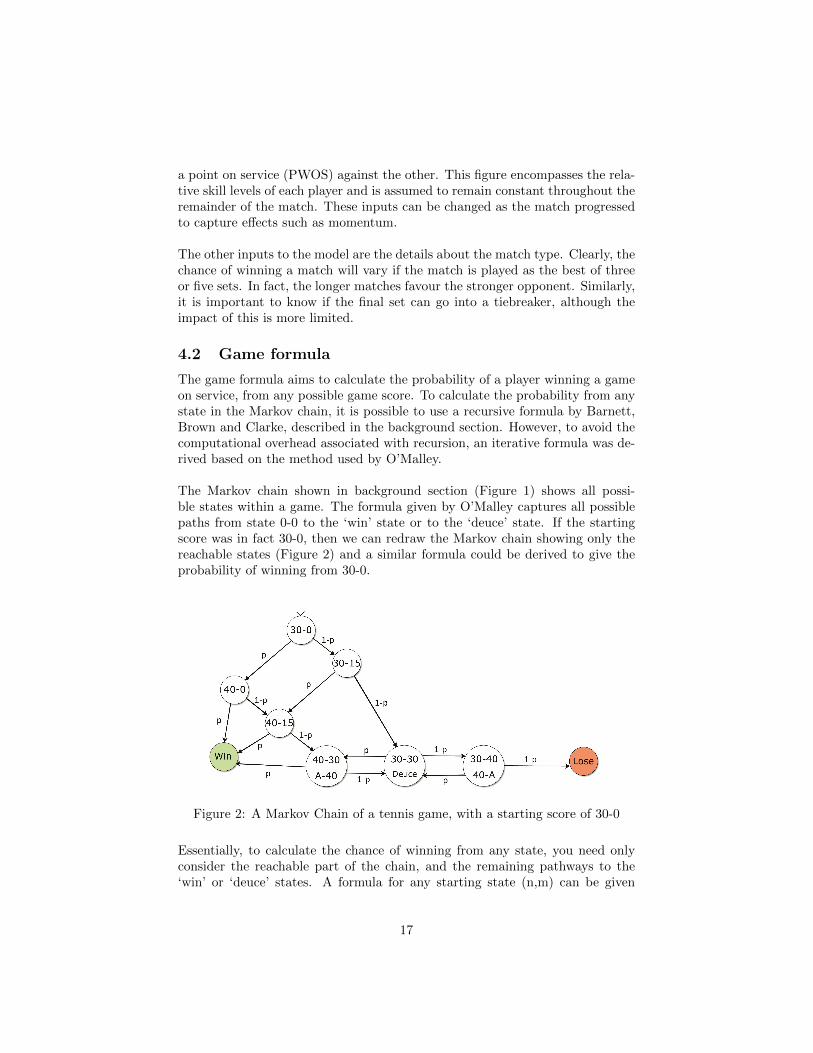
The game formula aims to calculate the probability of a player winning a gameon service, from any possible game score. To calculate the probability from anystate in the Markov chain, it is possible to use a recursive formula by Barnett,Brown and Clarke, described in the background section. However, to avoid thecomputational overhead associated with recursion, an iterative formula was de-rived based on the method used by O’Malley.
The Markov chain shown in background section (Figure 1) shows all possi-ble states within a game. The formula given by O’Malley captures all possiblepaths from state 0-0 to the ‘win’ state or to the ‘deuce’ state. If the startingscore was in fact 30-0, then we can redraw the Markov chain showing only thereachable states (Figure 2) and a similar formula could be derived to give theprobability of winning from 30-0.
Figure 2: A Markov Chain of a tennis game, with a starting score of 30-0
Essentially, to calculate the chance of winning from any state, you need onlyconsider the reachable part of the chain, and the remaining pathways to the‘win’ or ‘deuce’ states. A formula for any starting state (n,m) can be given
17

as follows. It is then easily implemented using a for loop in Java and can beoptimized by pre-calculating the coefficients.
PG(n,m) =
2−m∑i=0
(3− n + i)!
(3− n)!× i!p4−nqi +
(6− n−m)!
(3− n)!× (3−m)!p3−nq3−mp(d) (9)
Where p(d) is the probability of winning from deuce, p is the probability ofwinning a point on service and q = 1− p. It is also necessary to specify n andm in terms of the number of points won (eg 1-0, 3-3), and not the traditionaltennis scores of 15, 30, 40 etc. Also, A-40 and 40-A are equivalent (analytically)to scorelines 3-2 and 2-3 and the latter must be used.
An example case where player A has a win on serve probability of 0.6227 yieldsthe following probabilities.
Score 0 15 30 40 game
0 0.781 0.629 0.417 0.177 0
15 0.873 0.757 0.563 0.284 0
30 0.944 0.875 0.732 0.456 0
40 0.986 0.962 0.899 0.732 -
game 1 1 1 - -
Table 1: A table showing the probabilities of a player winning a game from anypossible scoreline. The opponents score is shown on the horizontal axis
4.3 Set formula
Creating an iterative formula for the set probabilities is more complicated. Thisis due to the fact that service alternates between the two players. For example,from the state 0-0 games each, there are many ways to reach, for example, state6-4. Player one could break once, and player two not break at all, player onecould break twice and player two once etc. To cover all possibilities you wouldthen need to consider the permutations for each scenario (i.e. player breaks inthe first game, second game and so on).
For simplicity, the recursive approach outlined by Barnett, Brown and Clarkewas used for calculating set probabilities[9]. To help speed up the computation,memoization was used. This involved caching already calculated results in anarray to remove the need for any recursive function calls. This required initial-izing all absorbing states in the Markov chain with either 0 or 1 (depending onif the scoreline represented the player having already won or lost the set) anditerating the Markov chain from bottom to top such that the probabilities ofboth the child nodes were calculated before the parent node.
18

There was also a special case for state 6-6. As mentioned earlier, the rulesof tennis are that the set will be decided by a tiebreaker (provided it is not thefinal set of a match specified not to have a final set tie-break). The probabilitiesfor a tiebreaker were calculated in a similar manner to those of a set due to theirresemblance and these had to be calculated before the set probabilities. TheMarkov chain for the tiebreaker was made finite using an infinite summationapproximation as used similarly in the game formula for the deuce state.
For a match between two players A and B, with probabilities of winning onserve as 0.6227 and 0.6359 respectively, the chances of player A winning a set(Table 2) and tie-break (Table 3) from different score-lines are as follows (as-suming player A serves the first game of the set).
score 0 1 2 3 4 5 6
0 0.456 0.232 0.178 0.05 0.026 0.002 0
1 0.518 0.459 0.213 0.153 0.032 0.011 0
2 0.764 0.528 0.462 0.187 0.12 0.014 0
3 0.83 0.799 0.54 0.466 0.149 0.072 0
4 0.961 0.871 0.844 0.555 0.47 0.092 0
5 0.987 0.984 0.925 0.907 0.576 0.473 0.093
6 1 1 1 1 1 0.58 0.478
Table 2: A table showing the probabilities of a player winning a set from anypossible game score. The opponents score is shown on the horizontal axis.
score 0 1 2 3 4 5 6 7
0 0.478 0.334 0.251 0.173 0.076 0.022 0.006 0
1 0.566 0.48 0.387 0.232 0.108 0.052 0.016 0
2 0.716 0.641 0.481 0.307 0.206 0.115 0.025 0
3 0.845 0.739 0.587 0.483 0.365 0.169 0.04 0
4 0.91 0.831 0.769 0.688 0.484 0.247 0.11 0
5 0.959 0.939 0.91 0.811 0.628 0.486 0.303 0
6 0.993 0.989 0.97 0.922 0.877 0.806 0.486 0.177
7 1 1 1 1 1 1 0.673 0.486
Table 3: A table showing the probabilities of a player winning a tiebreaker fromany possible score. The opponents score is shown on the horizontal axis.
19

4.4 Match formula
A formula for deriving the probability of winning a match from any state canbe derived using similar principles to those used in the game formula and henceavoids the need for recursion or memoization. Whilst the probability of winninga game, set or tiebreaker is independent of the match type, the match formularequires extra inputs. Specifically, the number of sets required to win the matchand whether or not the final set will go to a tiebreaker. From a set score of (n,m),the formula is as follows.
• Let k be equal to 1 in the case of no final set tiebreaker and 0 otherwise
• Let psT be the probability of the player winning a tiebreaker set
• Let s be the number of sets required to win the match (2 or 3).
For the case k = 0 the following formula gives the full result.
P (n,m) =
s−2−m+k∑i=0
(1 + s− 1− n)!
((s− n− 1)!× i!)(psT )s−n(1− psT )i (10)
If k = 1, then the result from the previous formula is added to the result of thefollowing formula (to deal with the differing probabilities of winning a tiebreakerset and a non tiebreaker set).
• Let j be equal to 4 if s = 3 and 2 otherwise
• Let ps be the probability of the player winning a non tiebreaker set
(j − n−m)!
(s− 1− n)!× (s− 1−m)!(psT )s−n−1(1− psT )s−1−mps (11)
Although the formulas look complicated, this is largely due to number of con-ditions required when working out the permutation coefficients (i.e. number ofpossible paths to the ‘win’ state). Essentially, you take the number of sets playerone requires to win, the number of sets player two can win without winning thematch, and sum the probabilities of all possible combinations that result inplayer one winning the match.
Table 4 shows some example probabilities for a best of 5 set match involvingplayers with win on serve probabilities 0.65536 and 0.6452. The probabilitiesare given without a final set tiebreaker and with (without/with).
20

score 0 1 2 3
0 0.553/0.552 0.357/0.355 0.148/0.147 0/0
1 0.729/0.728 0.543/0.542 0.28/0.278 0/0
2 0.895/0.895 0.778/0.777 0.531/0.528 0/0
3 1/1 1/1 1/1 -/-
Table 4: A table showing the probabilities of a player winning a match fromany possible set score.
4.5 Service faults
On service you are allowed one ‘fault’ if the first serve breaks any rules. If aplayer receives two faults on a single point, then the point is forfeit. For thisreason, tennis players commonly play two types of serve. On their first serve,a stronger but less reliable serve is attempted. If it fails, then a second serve,which is far more reliable but generally easier to return is performed.
The probability of winning a point on a first serve is increased due to thedifficultly of returning a more powerful serve, and the increased possibility of anace. The receiving player can often be put immediately on the back foot witha good serve. A second serve is commonly easier to return, and so some of theadvantage gained by having service is lost.
Until now, we have assumed a single value for the percent chance of winning apoint on service. However, if a fault occurs this is not always the case and themodel should take this into account. To do this, the input parameters to themodel are changed to the following.
• P (noFault) -The probability a player’s first serve not faulting
• P (win|noFault) -The probability a player will win the point if the firstserve does not fault
• P (win|fault) -The probability a player will win the point on his secondserve
The probability of winning a point on service is therefore given by
P (win) = P (noFault)P (win|noFault) + (1− P (noFault))P (win|fault) (12)
For an example player with P (noFault) = 0.70, P (win|noFault) = 0.64 andP (win|fault) = 0.55, then
P (win) = (0.70× 0.64) + (1− 0.70)0.55 = 0.613
21

If the first serve faults, however, this becomes
P (win) = 0.55
A service fault can therefore have a moderate effect on the probability of winningthe match. For more important points, we can speculate that service faultsshould be significant enough to warrant a noticeable change in the betting odds.By incorporating faults into the model, we can estimate how the odds wouldchange if a fault occurred and potentially infer service faults from the live marketodds.
4.6 Implementation of the Model
As the scoring system of tennis is a hierarchical Markov chain, to calculate theprobability of a player winning the entire match requires using a combinationof the aforementioned formulas. This typically involves the following procedure
• Let P (cGame) is the probability of winning the current game
• Let P (cSet) is the probability of winning the current set
P (cSet) = P (cGame)P (win set | current game won)
+ (1− P (cGame))P (win set | current game lost)
P (win match) = P (cSet)P (win match | current set won)
+(1− P (cSet))P (win match | current set lost)
There are several variants to this formula, for example where the match is ina tiebreaker. However, the same general principle holds. We first considerthe effect of the next point, and then consider how the point can affect thegame/tiebreaker, set, and match. With the notification of a service fault, thenthe probability of winning the next point is simply changed to P (win|fault).
Once the model was finished, a GUI (Figure 3) was created to provide an easyto use interface and a possible gambling tool.
4.7 Simulator
Under the same assumptions as the mathematical model, a less elegant way tocalculate the odds from a particular scoreline would be to ‘simulate’ the outcomeof a match using random number generation. Given the same input parameters(match type, current scoreline and probability of the players winning a pointon their respective serve) it is possible to compare the probabilities of a playerwinning a point against a uniformly distributed random variable in order to de-termine which of the two players wins the current point. This can be repeatedmany times, keeping track of the current score until the match is eventually
22

Figure 3: Tennis Calculator GUI
finished.
If multiple matches are simulated, you can get an accurate estimation for theproportion of matches you would expect a player to win from any startingscoreline or input parameters. However, there are obvious disadvantages to thismethod. The main problem is the large amount of computation required toget accurate results. Given that the accuracy of the result is important, onecould suggest that tens of thousands of matches should be simulated from eachpossible starting scoreline. In such a time critical application where knowinghow the odds will change is important, it does not make practical sense to simu-late every result and a faster way to generate probabilities on the fly is necessary.
A simulator, however, was created and used to some capacity when testingthe system. Due to the nature of the program, testing was extremely importantas an incorrect figure could result in mis predictions in score and even erroneousbets. The complex nature of the tennis scoring system and mathematical for-mula meant it was difficult to guarantee that the mathematical models werein fact giving the desired results. Fortunately, creating a simulator was morestraightforward and was thus used to compare results against those derived fromthe mathematical model.
23

The simulator itself can be configured to any type of tennis match (3/5 sets,final set tiebreaker etc.) and for any input parameters. For a given set of in-put probabilities, the simulator iterates through every reachable state during atennis match and performs a specified amount of match simulations. Severalsimulations are run from each state to cover all possible match types (e.g. theinclusion or omission of a final set tiebreaker) and the situations where therehas or has not been a service fault on the current point.
It is safe to assume that if the results are correct for one set of plausible in-put probabilities, then the model can be verified for all possible variations ofthe input probabilities. After changes were made to the mathematical model,the output was compared to the simulated results and it was ensured that theyremained similar to within an arbitrarily small number. This process helpedeliminate several minor errors such as missed boundary conditions and thusproved to be useful. It also gave a necessary level of confidence in the model.
4.8 The importance of a point
The importance of a point is considered a measure of the extent to which thepoint will influence the chance of each player winning the match. Due to theunique scoring system of tennis, the importance of points can vary massivelythroughout the duration of a match depending on the current scoreline. Thisobviously has a direct influence on the odds expected for each player after thepoint is decided.
For example, in a match where both players are tied at two sets and four gamesall, any point could be considered critical. If the score of the current game was*30-40, then the server(indicated by the asterisk) would be facing a break point.In the event of losing the point, it would seem very likely that the entire matchwould be lost. If we assume both players are identically matched (same winon serve percentage of 0.65) then the derived model would speculate odds of2.964 before losing the point, and 12.283 afterwards. Clearly, this is a high im-portance point and we would expect to see a large jump in the odds from Betfair.
The other extreme would be if a player was already two sets, and four gamesup against the opponent. The match is, for all intents and purposes, alreadyover. The chance of the other player getting back into the game is so low that inmost cases bets would no longer be taken on the event. With a similar scenarioto that above, the odds would change from 1.013 to 1.026. This would seem tomake inferring the score more diffcult, as the change in odds would be extremelysmall.
24

5 Comparison between Model and Live Odds
In this section, several matches from the 2011 French Open are examined. Thepoint by point score of each game was recorded, and fed into the derived math-ematical model to determine the odds for each player as the match progressed.These odds were then graphed against the last priced matched data retrievedfrom Betfair and comparisons were made to see how closely the derived modelmatched the market data.
In each case, the win on serve percentage input parameters of the model wereestimated such that the initial odds generated by the model were as similar aspossible to the projected odds calculated from the Betfair data at the very startof the match. It is then also taken into account that the probability of win-ning a serve is generally lower for womens matches and higher for mens. Theseparameters remain constant throughout the entire match.
5.1 Schiavone V Li
The first match discussed is the 2011 Womens French Open final between Schi-avone and Li, in which Li beat Schiavone two sets to zero. Going into the match,it was deemed to be a very close encounter. The projected odds before the matchbegan were 2.144 for Schiavone and 1.875 for Li, making Li the favourite with a53.33 percent chance of victory. During the match over 15 million pounds wastraded making this a fairly highly traded match and potentially a more stablemarket.
The model used assumed that the probability of Schiavone winning a pointon service was 0.582, and similarly 0.5884 for Li. To see a greater variationin odds, we plot Schiavone’s last priced matched against time. We also ignorethe last few points of the match, where the odds spike upward and distort thegraph. (Figure 4 overleaf)
25

Fig
ure
4:L
iv
Sch
iavo
ne
-S
chia
von
e’s
last
pri
ceM
atc
hed
again
stti
me
26
From the graph, it is immediately clear that there is a strong similarity betweenboth sets of data, with significant overlap between the two lines. Based on this,it would seem likely that other Betfair users are using a similar model to pre-dict the outcome of a match and are placing bets accordingly. However, thereare still areas where the odds differ quite dramatically, even though the basicpatterns of movement are similar.
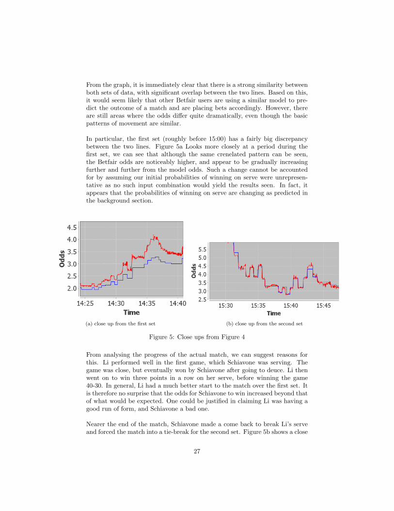
In particular, the first set (roughly before 15:00) has a fairly big discrepancybetween the two lines. Figure 5a Looks more closely at a period during thefirst set, we can see that although the same crenelated pattern can be seen,the Betfair odds are noticeably higher, and appear to be gradually increasingfurther and further from the model odds. Such a change cannot be accountedfor by assuming our initial probabilities of winning on serve were unrepresen-tative as no such input combination would yield the results seen. In fact, itappears that the probabilities of winning on serve are changing as predicted inthe background section.
(a) close up from the first set (b) close up from the second set
Figure 5: Close ups from Figure 4
From analysing the progress of the actual match, we can suggest reasons forthis. Li performed well in the first game, which Schiavone was serving. Thegame was close, but eventually won by Schiavone after going to deuce. Li thenwent on to win three points in a row on her serve, before winning the game40-30. In general, Li had a much better start to the match over the first set. Itis therefore no surprise that the odds for Schiavone to win increased beyond thatof what would be expected. One could be justified in claiming Li was having agood run of form, and Schiavone a bad one.
Nearer the end of the match, Schiavone made a come back to break Li’s serveand forced the match into a tie-break for the second set. Figure 5b shows a close
27

up of the graph when the current score is roughly five games all. The modeland Betfair odds in this case are remarkably similar suggesting that Schiavone’sresurgence has altered the current win on serve probabilities to closely matchour original prediction. The importance of each point near the end of the gameis also increased, and the changes in odds are much more apparent as the matchnears it’s completion.
From this graph alone, is is easy to give a general outline of the match. Schi-avone must have lost the first set and was broken in the second to create thespike around 15:20. She then will have broken back causing the second set tofinish closely with a tiebreaker sealing the victory for Li. Overall, there aremany areas were a jump in odds is clearly visible, indicating that inferring thescore should be possible to at least some extent.
5.2 Schiavone V Bartoli
The next match is the 2011 French Open womens semi-final between Bartoliand Schiavone which saw roughly 14 million pounds traded. This match wasanother two set to nil victory, this time in Schiavone’s favour. Going into thematch, it was deemed to be more one-sided with odds of 2.68 for Bartoli and1.591 for Schiavone. The same graph as before is plotted (figure 6)
Again, the same general pattern can be seen, with both lines appearing similar.We would therefore also expect to be able to determine the score for much of thegame. The slight difference being that perhaps the model varies more greatlyfrom the actual Betfair odds. In a similar manner to the Schiavone/Li match,we can explain the changes in odds from a point by point analysis of the match.
Bartoli had good form on service winning her first three service games: 4-0,4-1 and 4-0. This would easily explain the gradual lowering of the odds belowthose of the model during the first half of the graph. This gap changed to anextent when she was broken and eventually lost the first set. Nearer the endof the match, the odds are instead significantly higher that the model. We canaccount for this as Bartoli was a set and break down due to a run of poorerform. As well as being non-favourite to begin with, it is easy to understandwhy not many would be willing to back Bartoli to make a comeback from thissituation.
28

Fig
ure
6:B
arto
liv
Sch
iavo
ne
-B
art
oli
’sla
stp
rice
Matc
hed
again
stti
me
29

5.3 Murray V Nadal
This match is the men’s semi-final from the 2011 French Open. Compared tothe previous games this match was far more one sided from the start, saw moremoney traded (25 million) and was also a best of five sets instead of three. Mur-ray, the eventual loser in straight sets, was only given roughly a 0.143 chanceof winning against Nadal. Parts of the last priced match graph for Murray areshown in Figures 7 and 8.
Figure 7: Murray last priced match graph - middle period of match
Figure 8: Murray last priced match graph - end period of match
30

These portions of the graph are far more noisy than the previous matches. Fig-ure 8 especially is almost completely useless for inferring any sort of detail aboutthe match at hand. There are two reasons for this. One reason is simply thatthe odds are in general much higher than those seen in the previous matches. Asthe odds increase, so does the boundary between values allowed on the Betfairexchange.
The next reason is due to the cross-matching algorithm described previously.Whilst cross-matching is useful, and theoretically gives us the true last pricedmatched, it would seem in this case to be a hindrance. Figure 7 shows that youcan see a lot of fluctuation between the odds of 101 and 51. These values mapto odds of 1.01 and 1.02 matched on Nadal. In this case, we can see that themoney matched on Nadal is interfering with the last priced match for Murray.
By plotting the highest back price available for Murray, we see a completelydifferent picture. Figure 9 gives a much more detailed and informative pictureon how the odds are changing. This suggests that when the odds increase be-yond a certain level, the last priced matched should not be used and instead theodds and amounts available on each player should be considered.
Figure 9: Murray highest back odds available - end period of match
31

5.4 Determining PWOS probabilities from ‘in-play’ odds
In the tennis model, the PWOS probabilities determine the players chance ofwinning from the current state of the match. Therefore, by finding where theodds have settled after a point, we can estimate what the PWOS must currentlybe to offer the current match odds, given the latest odds and score-line. In thissection, the PWOS probabilities are calculated from the Betfair data whilst therecorded score feed is used to determine when points have been won.
After each point, the average of the last priced matched (or highest availableprice for high odd values) was taken for a short period after the point was re-solved. This value was then used for the recalibration. If the point was won bya player, it is assumed that their PWOS will not decrease, but instead mightincrease. Conversely, losing a point should not raise the players PWOS value asfor either case this would contradict the idea of momentum.
Given the current estimate for the PWOS probabilities, and based on the abovelogic, the current estimates were slightly increased or decreased by a small factorand placed into the tennis model. The combination of PWOS probabilities thatpredicted the odds closest to their actual value then replaced the current esti-mations. The graph showing the results from this analysis on the Schiavone/Limatch is shown in Figure 10.
Figure 10: Schiavone V Li - estimated PWOS values throughout the match
At the start of the match, we know that Li was the better player, dominatingmuch of the first set. Therefore, it is no surprise that the initial period of thegraph shows the PWOS values separating apart. Relating this to the compari-son graph (Figure 4), this would explain the model odds being an underestimateof the actual odds. It is also no surprise that the nearer the end of the match,when Schiavone made her comeback, that the PWOS values are much closer tohow they were at the beginning of the match.
32

However, during the middle of the match, the PWOS values do not vary asexpected, with Schiavone’s PWOS increasing rapidly. This also coincides witha period during which Schiavone’s odds were high. In this case, going on thehighest available back price for higher odds would generally gave a slightly lowervalue than expected. This would account for the increase in Schiavone’s PWOSas the lower odds would seemingly improve Schiavone’s predicted chance of win-ning.
The accuracy of this PWOS method would therefore seem to drop when theodds are high, but offers a good approximation at lower odd levels. For higherodds, it is difficult to know exactly where the true odds would lie. This is be-cause as the odds increase, the boundary between accepted odds values becomeslarger and the amount of money traded decreases rapidly. If for example, thetrue odds were 15.4, the nearest odds boundary allowed by Betfair would be 15.When calculating PWOS values this would have a significant effect. Essentially,it becomes almost impossible to estimate the true odds in this case.
33
6 Inferring the score
From all of the comparison graphs, it is clear that to a large extent the modelodds are very similar to the market data retrieved from Betfair. Based on this,it would seem likely that other Betfair users are using a similar model to predictthe outcome of a match and are placing bets accordingly. It should thereforebe possible to infer the score from the live ‘in-play’ odds. However, it is alsoclear that the derived odds vary at times to the Betfair odds due to the idea ofmomentum and possibly other factors.
In this section, several algorithms for trying to determine the score of a matchfrom the live betting odds are suggested. The reasoning behind each approachis explained and each is tested on a variety of matches. The results are thenanalysed to see why the method was successful or unsuccessful and based onthe results, the algorithm is refined in each step.
7 Non-corrective bounds checking
7.1 Method
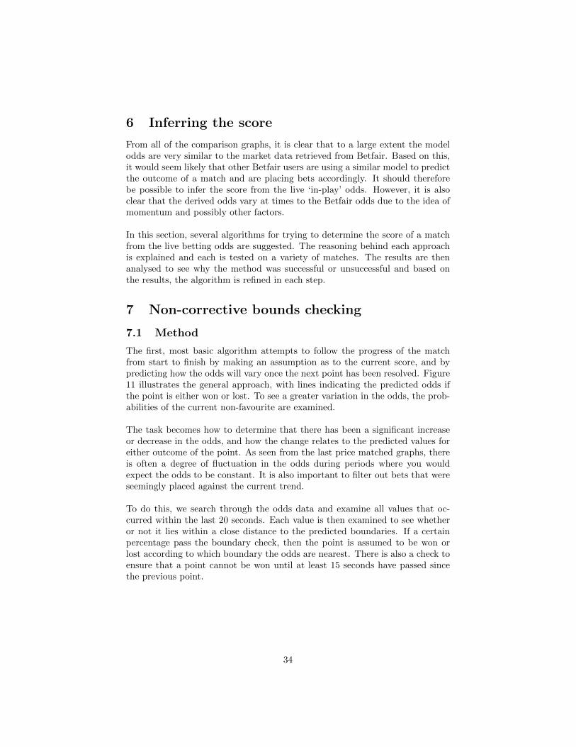
The first, most basic algorithm attempts to follow the progress of the matchfrom start to finish by making an assumption as to the current score, and bypredicting how the odds will vary once the next point has been resolved. Figure11 illustrates the general approach, with lines indicating the predicted odds ifthe point is either won or lost. To see a greater variation in the odds, the prob-abilities of the current non-favourite are examined.
The task becomes how to determine that there has been a significant increaseor decrease in the odds, and how the change relates to the predicted values foreither outcome of the point. As seen from the last price matched graphs, thereis often a degree of fluctuation in the odds during periods where you wouldexpect the odds to be constant. It is also important to filter out bets that wereseemingly placed against the current trend.
To do this, we search through the odds data and examine all values that oc-curred within the last 20 seconds. Each value is then examined to see whetheror not it lies within a close distance to the predicted boundaries. If a certainpercentage pass the boundary check, then the point is assumed to be won orlost according to which boundary the odds are nearest. There is also a check toensure that a point cannot be won until at least 15 seconds have passed sincethe previous point.
34

Figure 11: Boundary checking method illustration
7.2 Dealing with non-iid points
From the earlier comparison graphs, it becomes apparent that the derived modeldoes not follow the Betfair odds exactly due to influences such as momentumand possibly other non-obvious factors. Therefore, to adapt the model to thecurrent market after each point is played, the Betfair data is examined and usedto create the next set of boundary values.
Once it has been determined that a point has been won or lost, the first stepis forming an estimation of the ‘new’ odds once the market has settled. Whenenough values meet the boundary check, then the time of the earliest value toenter the boundary is recorded to try and give the exact time of the point. Thealgorithm then waits for several seconds and takes an average of the values forthe period following the change. This attempts to create a more true value whenthere is variation in the odds.
It is also not possible to assume that the win on serve percentages (WOSP)will remain constant as shown earlier. To combat this and to make the algo-rithm more robust, code was created to generate a wide range of possible winon serve percentage (WOSP) combinations that would give the same odds for agiven scoreline. The list of possible WOSP combinations was then iterated andeach entered into the tennis model to get the expected odds if the next pointwas won or lost.
By taking the minimum and maximum values for each case, essentially, given acurrent scoreline, there were four values determining the ranges over which we
35

would expect the odds to lie in-between after the current point had completed.Figure 12 illustrates the updated method. It was then possible to say with a fairdegree of certainty that the odds would lie between either of the two boundaryareas when the point was resolved.
Figure 12: Boundary checking method illustration
However, there is also the possibility that the odds will not vary according to themodel, even if all possible PWOS combinations are considered. Whilst this isunlikely for the majority of points, there is nothing to stop the odds not chang-ing as much as they should, or vice versa, for a particular point. A possiblereason would be that the predicted odds lie in-between a set of a odds valuesallowed by Betfair (i.e. 4.4 and 4.3 are allowed, but 4.33 is not). Because ofthis, there are varying degrees of leniency allowed in the boundary check.
Given the predicted current odds, using the lose(min) and win(max) values,the minimum expected increase and decrease is calculated. Typically, if theodds being checked are at least 0.80 times the expected change then the valueis accepted as being inside the boundary. At higher odds, this value is relaxedslightly due to the greater distance between allowed odd values. For this versionof the algorithm, if the value lies above the lose(max) or below win(min) thenit is assumed to be within the boundary.
7.3 Odds information
So far we have not specified what data is being used when referring to the ‘odds’.The comparison section highlighted that depending on the value of the odds,different approaches might be necessary. Theoretically the last price matched
36

should give the most accurate representation as money being traded is the mostpowerful indication of the odds being at a particular value. However, we haveseen that the last priced match value becomes distorted by cross matching athigh odd levels.
The algorithm therefore uses the last price matched value, with cross-matching,as long as the odds remain under a certain value, i.e. 5. Once the odds goover this value, to get a more realistic overview of the market, a moving averagetotal of the last priced matched is used. This is an attempt to make up for thehigher boundaries between the odds and potential fluctuation between theseboundaries.
If the odds increase above 10, the highest back prices available are examinedto determine the odds. As the odds rise, the amount traded over the playergenerally goes down, so even without cross-matching, the last priced matchedover only the one player would still not be sufficient.To avoid distortion in thehighest back price available, the amounts available are also taken into account.
In general, the highest odds are ignored if the amount available is small, andsignificantly less than the amount offered at the next best odds. This is in anattempt to capture the activity of the automated traders, who will more likelybe using a similar model.
7.4 Results
The algorithm, as described in this section, was tested on the following matches.The results are displayed on graphs showing the odds used by the algorithm (lastprice matches, moving average or highest back price) with annotations pointingto the areas where the score is believed to have changed.
7.4.1 Bartoli V Schiavone
The graph (Figure 13) displays the first few games of the Bartoli/Schiavonematch. The score prediction is given with Bartoli’s score first in each case andappears initially to be accurate. Whenever there is a an upward shift in theodds, this is registered as a point for Schiavone, and the reverse is taken as apoint for Bartoli. In actual fact the only correct score-lines are the first fivepoints. The area circled in green causes a problem, and derails the algorithm.
From the graph, one could easily infer that a point has been lost, taking thescore to 0-15. This is what the algorithm detects, however, no such point waswon and so it would be expected for the odds to remain the same until the pointwas won by Bartoli. As the current score prediction is now wrong, the min/maxvalues are also invalid meaning the algorithm cannot always continue to goodeffect.
37

Figure 13: Bartoli last priced matched - score prediction
It is difficult to know what caused this unexpected change in odds. One possiblereason can be obtained from the particular line of commentary on the matchitself. ‘Schiavone comes to the net but sends an easy volley into the net’ [5].Perhaps from watching the game, users expected Schiavone had already wonthe point as the volley presented itself and decided to take a quick bet beforethe odds changed. A strategy that obviously would have backfired.
Another possible cause would be acknowledging the fact that the match wasstill in its infancy. Typically, we can expect that at the beginning of the matchthe odds will vary quite a bit from the behavior of a model. It is likely that atthe beginning of a match you would see a higher amount of users placing betswithout any modelling software. It is also possible that those using modelingsoftware are recalibrating based on the current activity or perhaps still waitingto begin trading any money.
For instance, the first game could be used to gauge who is serving first, suchinformation is critical to the model and is not readily available. This could beinferred by looking at how the odds changed during the first game. Alterna-tively, the amount by which the odds changed could also be used to work outa rough estimate for the PWOS figures in order to begin trading. The fluctua-tions around the gap after the second game (to the right of where the score ispredicted as 40-15) strengthens this theory.
38
7.4.2 Schiavone V Li
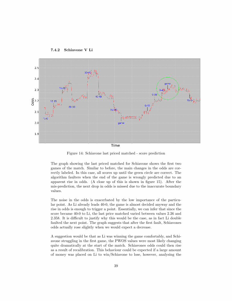
Figure 14: Schiavone last priced matched - score prediction
The graph showing the last priced matched for Schiavone shows the first twogames of the match. Similar to before, the main changes in the odds are cor-rectly labeled. In this case, all scores up until the green circle are correct. Thealgorithm faulters when the end of the game is wrongly predicted due to anapparent rise in odds. (A close up of this is shown in figure 15). After themis-prediction, the next drop in odds is missed due to the inaccurate boundaryvalues.
The noise in the odds is exacerbated by the low importance of the particu-lar point. As Li already leads 40-0, the game is almost decided anyway and therise in odds is enough to trigger a point. Essentially, we can infer that since thescore became 40-0 to Li, the last price matched varied between values 2.26 and2.358. It is difficult to justify why this would be the case, as in fact Li doublefaulted the next point. The graph suggests that after the first fault, Schiavonesodds actually rose slightly when we would expect a decrease.
A suggestion would be that as Li was winning the game comfortably, and Schi-avone struggling in the first game, the PWOS values were most likely changingquite dramatically at the start of the match. Schiavones odds could then riseas a result of recalibration. This behaviour could be expected if a large amountof money was placed on Li to win/Schiavone to lose, however, analysing the
39

amounts matched shows this is not the case.
The opening game in this case was fortunate to be a closely contended one,causing a large variation in odds for each point. However, it is still clear thatthe first game is rather erratic with the odds changing significantly betweenpoints. Although at 30-30 the slight rise could be attributed to a Schiavoneservice fault, this does not explain the large variation after the score goes to15-30 and 30-40.
Figure 15: Schiavone V Li score prediction - close up of error
7.4.3 Murray V Nadal
Figure 16: Murray V Nadal beginning of match
40

Figure 16 is different to the other graphs as the odds are much higher, mean-ing a moving average of the last priced match is used. The actual end of thefirst game is indicated by the green circle, with the 0-15 prediction before thatreferring to a point won by Nadal when the game was 40-0 to Murray. Theodds then proceed to drop after Murray has won the game, but surprisingly riseagain inside the green circle when the players were changing ends.
Looking at other indicators, such as the highest back price for Murray, showsthat when Nadal won a point to take the first game to 40-15 there was no changeat all. In fact, the period just before and after the game is won by Murray israther inconclusive even when looking at all the information available. The lastprice matched value appears to vary from 6.2 to 6 throughout, whilst the high-est back prices indicate that the odds of Murray winning also rise shortly afterMurray wins the game.
7.4.4 Total amount matched
To analyse the amount of money traded during the Murray/Nadal match, thedifferences in the total amount matched on the event were taken between suc-cessive calls to the Betfair API every second. The resulting graph (figure 17)shows the amount traded at each particular point during the Murray/Nadalmatch. Other matches also gave a similar picture
Figure 17: Murray V Nadal amount matched analysis
41
What is immediately apparent is that during certain areas of the match, anextremely large amount is traded very suddenly. This would seemingly be theresult of a single user deciding to make a very large bet. For example, at around5:12, over £380,000 is placed on Nadal to win. Due to the sheer volume, therewas simply not enough money being offered at the highest available odds of1.11. Therefore some of the money was traded at the odds of 1.11, some at 1.1and the rest at 1.09.
A similar spike can also be seen nearer the beginning of the match. In fact,a large £200,000 bet was placed on Nadal during the first game, the same atwhich Nadal won his first point that was missed on the previous graphs. In gen-eral, it is easy to see that such a pattern of bets will directly influence the oddsand may cause brief periods of unusual activity as the market reacts to such anevent. This may offer an explanation for the seemingly anomalous movementin the odds.
7.5 Conclusions
As shown in the score prediction graphs, the algorithm is largely successful atpredicting when a point has been won or lost. However, due to the scoringsystem of tennis, even one missed or erroneous point can have a huge effect onthe prediction of the next points. If the end of a particular game is not trackedcorrectly, then the error carries through and the algorithm derails, becomingineffective.
It does show, however, that it is possible to avoid the need to add non-iddaffects into our model by extracting the information from the bets placed byother Betfair users. Given the odds and score, we can infer roughly what theprobabilities of win on serve should be and hence re-adjust the boundary valuesfor the next point. This is advantageous, as there may be factors that cannotbe inferred from the pattern of points played alone, such as: a player may havepicked up a slight injury concern, is serving poorly, or if there is a gradual in-crease in the number of people backing a certain player.
Overall, the algorithm highlights the essential ability for error correction foraccurate long term score prediction. Several potential sources of anomalies inthe odds were suggested. These may arise at any time and must be dealt with.For example, those introduced by the calibration of modelling software, a largeamount of money being traded at once, or points where the player is largelyexpected to win but in fact makes a mistake.
42

8 Error correction - Breaks in play
In this section, a method of detecting and correcting an erroneous score predic-tion is detailed. The aim being to utilise scheduled breaks in play to performscore ‘check-pointing’. Firstly, a brief background on the rules and regulationsof rests within a tennis match is given. The reasoning behind the check-pointingidea is then explained, and the algorithm described in detail. Using this levelof error correction, the previous matches are revisited and the affects of thealgorithm are examined.
8.1 Rests
Tennis matches can often last for several hours. It is therefore essential theplayers have a rest at certain intervals, typically when the players change ends.During the match, the players change ends at the end of every first, third andevery subsequent odd game. If the set finishes, and the number of games playedis odd, the players change ends at the end of the set. Otherwise, they changeends after the first game of the set.
The International Tennis Federation rules state that players may rest duringthis change in ends in accordance to the following passage.[2]
When the players change ends at the end of a game, a maximumof ninety (90) seconds are allowed. However, after the first game ofeach set and during a tie-break game, play shall be continuous andthe players shall change ends without a rest. At the end of each setthere shall be a rest break of a maximum of one hundred and twenty(120) seconds.
8.2 Explanation
It is inevitable that during a match, there will be many such periods of rest.Given that these break periods are from the moment that a point finishes untilthe next serve is performed, we can expect that during this period there shouldbe no reason for the odds to vary significantly. Therefore, we can aim to detectthese gaps in play and use them to our advantage.
To test for these gaps in play, the time difference between the last registeredpoint and the current time is taken. If this time is large (i.e. 85 seconds ormore), then the odds during this period are iterated over. As the boundaryvalues could be wrong, the odds are checked for any significant change thatmight indicate a point having occurred. Figure 18 shows an selection of theSchiavone/Li odds graph, identifying two break periods.
Another check is performed by the break in play predictor, which keeps track ofthe time of the last check-point (or start time of the match if no check point has
43

Figure 18: Schiavone V Li - breaks in play
occurred). If the time difference between successive breaks is not long enoughto allow a two games to be played, then the break is rejected. If a check-pointis detected, and a player is able to win the set by winning the next game, thenthis condition is reduced to one game. Similarly, if a new set is detected it isincreased to three games to accommodate the extra game before a rest.
Given the pattern of rests, it is possible to assume that the total number ofgames completed in the current set should be odd if a rest is detected. The firstbreak of the set should come at three games, then five, then seven and so on. Theonly exception is when a set has finished, and the score should be zero games all.
The algorithm essentially works on the basis that each check-point providesan exact prediction of the scoreline. Beginning with the start of the match, ateach check point the score and current odd information is recorded. At the nextcheckpoint, this information is revisited and used to verify the scoreline that iscurrently predicted, or help correct the score if it is wrong.
If all checkpoints can be detected, then essentially you can ‘refresh’ the scoreevery few games. In this case, the algorithm should be very effective in keepingtrack of the game score. This is due to there only being a few possible scenariosthat can occur between each check-point. For example, consider a period of thematch in which two games are played before another rest. The players can eitherboth hold serve (and the odds will remain similar to the previous check-point),or one player could break the other causing a much greater shift in the odds.
44

At each checkpoint, the odds and score from the previous check-point are en-tered into the model. The current odds taken from Betfair are then comparedagainst the model’s prediction for the different possible game score combina-tions at the current check-point. For example, if the previous check-point wasat two games to one, then we can determine which of the possible score-lines(4-1, 3-2 or 1-4) matches the current odds the closest.
So far, it has been implied that every check-point can be detected. The problemswith this method arise when the majority of check-points cannot be detected.As the number of games between detected check-points increases, the accuracyof the method depletes due to the dynamically changing PWOS. Some score-lines also have very similar odds (eg, 2-3 ,3-4, 4-5) and could easily be confused.
Due to the fact that there is a large variation in the possible lengths of a game(i.e. winning to nil compared to going to deuce several times) it is also difficultto tell how many games should have been played by only looking at the timeelapsed. For example, if the last check-point was 40 minutes ago, then therescope for a large variation in the number of games played, creating another dif-ficulty.
To try and help determine the number of games played between checkpoints,the predicted score is used. In general, from the original bounds checking al-gorithm, when a mistake occurs, errors begin to manifest as new points aremissed. This tends to slow the predicted progress of the match. Therefore, onetechnique is to round up to the next scoreline which would yield a break in play.If the nearest prediction using the model is far off, then the number of games isincreased further.
8.3 Results
8.3.1 Schiavone V Li
The Schiavone/Li match was largely successful under this method. A total ofseven checkpoints out of a possible ten were correctly identified which can beattributed to the success of the predictions. The end result was that the ma-jority of the match was predicted correctly on a point by point basis, and thefinal score of each set was correct.
Out of the seven check-points, only one had to alter the score. The error wascreated due to the current score of the match causing the odds to change ratherinsignificantly. Since the previous checkpoint, the first game was served andwon by Li 40-0 and the second game was won 40-15, after reaching 40-0, bySchiavone. This particular scenario is difficult to track from the odds. Oncethe score reaches 40-0, even if either player wins the point the odds will changeonly a very small amount.
45

The scoring prediction when the error correcting check-point was reached wasthree games to four, two points all. This was rightly changed to four games tofive by the error correction algorithm. In fact, a few other points were missedfrom similar scenarios but in many cases the errors managed to hide and didnot effect the future score prediction after the current game had been resolved.
The entire first set is shown in several stages in figures 19 & 20. Check-pointsare marked as CP, followed by the predicted game score.
46

Fig
ure
19:
Sch
iavon
eV
Li
-fi
rst
set
scor
ep
red
icti
on
wit
hch
eck-p
oin
tin
g.
Th
eod
ds
plo
tted
corr
esp
on
dto
those
use
dby
the
algo
rith
m(i
.e.
mov
ing
aver
ages
wh
enth
eodd
sare
over
5et
c.)
PA
RT
ON
E
47

Fig
ure
20:
Sch
iavon
eV
Li
-fi
rst
set
scor
ep
red
icti
on
wit
hch
eck-p
oin
tin
g.
Th
eod
ds
plo
tted
corr
esp
on
dto
those
use
dby
the
algo
rith
m(i
.e.
mov
ing
aver
ages
wh
enth
eodd
sare
over
5et
c.)
PA
RT
TW
O
48

8.3.2 Bartoli V Schiavone
The Bartoli/Schiavone match also saw a great deal of success with the help oferror correction. Although only three breaks in play were detected, two of thesecheckpoints made minor corrections to enable to algorithm to continue effec-tively. Similarly to the Schiavone/Li match, the final set scores were correct,and much of the match saw flawless prediction.
There were two main errors in the predictions during the match, each having asignificant carry on effect. The first occurs just after the third game followinga break in play. Figure 21 shows how the real odds (red) varied against whatwe would expect expect using the model odds (blue). In this case, we see thereare seemingly two discrete ‘step’s taken by the odds (as indicated by the greencircle), when there should really only have been one.
Figure 21: Bartoli V Schiavone - A graph of Bartoli’s odds and a set of predictedodds, highlighting the source of an error after the third game
The algorithm therefore detects that two points have been won by Bartoli, andthe rest of the score prediction up until the next checkpoint is invalid becauseof this error. It is also worth noting that the checkpoint just prior was notdetected either. This is because the odds vary quite a lot from the beginning ofthe break period, up until the end. In fact, a point was awarded to Bartoli justprior to entering the green circle.
Interestingly, whilst this might be symptomatic of a sudden large bet, this isnot the case at all. In fact, comparatively very little was traded during thisperiod. Referring back to the comparison graph (Figure 6) we can suggest an-other reason for this activity in the odds. From the end of this game onwards,the model odds become noticeably higher than the real odds, even though theywere largely similar for the first part of the match. This can also be seen bystudying the beginning of figure 21.
This behaviour can be explained by accounting for Betfair users with mod-elling software. As already discussed in the comparisons section, Bartoli had a
49

much better start to the match. It appears as if this break in play was used forrecalibration purposes. Whilst we might expect this to be a more gradual pro-cesses, there appears to have been a rather rapid transition in the PWOS values.
The next error is of a similar vein, shown in figure 22. It also occurs dur-ing a break, this time between the first and second sets. This time, as Bartolihas lost the set, the odds slowly increase as expected, perhaps due to modelrecalibration as before. There is also a large bet of over £250000 placed atroughly 16:02:10 on Schiavone to win, this may also account for the change inodds as the market adjusts.
Figure 22: Bartoli V Schiavone - A graph of Bartoli’s odds and a set of predictedodds, highlighting the source of an error inbetween sets. The arrow indicatesthe end of the first set
This rise at the end of the break is sufficient enough to award an erroneous pointto Schiavone and again throws the algorithm off. Fortunately, the next possiblebreak in play after this anomaly is detected, three games into the set. Once theerror was successfully corrected to one game Schiavone, two games Li, the scoreis actually predicted with 100% accuracy for the remainder of the match.
Figure 23 shows the score prediction graph from the point of the error cor-recting checkpoint in the second set to the end of the match.
50

Fig
ure
23:
Bar
toli
VS
chia
von
e-
Gra
ph
ofB
arto
li’s
od
ds
wit
hsc
ore
pre
dic
tion
du
rin
gth
ela
tter
part
of
the
seco
nd
set
(th
eve
ryla
stp
oint
iscu
t-off
)
51

8.3.3 Murray V Nadal
The Murray/Nadal match predictions improved under the check-pointing method,but not as well as the other matches. There were periods where the score pre-diction was correct, but these were not of a great length. The number of errorsmade between check-points was generally increased due to the several reasons.Firstly, the match was the best of five sets, meaning the points were generally ofa lower importance throughout, making it more common for points to be missednearer the start of the match when Murray’s odds were at there lowest.
Secondly, Murray’s odds were also became very high, and as his chance ofwinning decreased, the quality of the odd data diminished. This is becausethe majority of money was being traded over Nadal, and we therefore had touse the highest available back prices for Murray. These did not give as gooda picture as the last priced match values used for the previous two matches.There were often large jumps seen in the data, making errors more common.
8.4 Conclusions
Using breaks as a way of correcting the score has shown to be useful. On manyoccasions, the importance of the point can become too low or an anomaly in theodds can occur at any moment. Even a single mis-prediction can have a knockon effect for the entire match using the current algorithm and the overall resultis poor.
Given a chance to correct an error, the original algorithm performed well, beingable to correctly predict the score of a match for a lengthy periods at a time.In the Bartoli/Schiavone and Schiavone/Li matches, the score predictions werevery accurate for the majority of the match.
However, the obvious downside of this method is that it does rely on beingable to infer the periods of rest within a match. If the number of breaks in playdetected is low, it is possible for large errors to occur. There is also a smallchance that a break could be predicted when no such break has occurred. Forexample, if there is a very long point, an injury break or other such events.Although unlikely, any of the above will heavily derail the score prediction al-gorithm.
8.4.1 Set Markets
Another way of determining the moment when a set is finished can also be in-ferred from the ‘set betting’ market. Betfair often allows users to bet on thewinner of a particular set, although in most cases, these set markets are poorlytraded compared to the match odds. From this, we also assume that the datawill not be very useful in determining the current score.
52

Whilst the set betting market would offer a good and conclusive idea as tothe end of a particular set, it was not used in this project. The reason beingthat to obtain the Set market data required further API calls which would haveeaten into the amount of requests allowed on the free API service, reducing theaccuracy of the match odd data.
9 Evaluation
Based on the background research, a model was created to predict the chanceof a player winning from any possible score-line reachable during a match. Themodel used several assumptions, as was common in relevant literature, such asthat each point would be independently and identically distributed. Once com-plete, a simulator was created to ensure the values were correct. The end resultwas a fully functioning tennis prediction model.
The analysis of the Betfair odds and those generated by the model showeda good level of similarity. This implied there was scope to relate the changesseen in the Betfair odds to the derived model and this was a crucial factor inbeing able to determine the score of a match in progress. This allowed theproject to continue, and inferring the score was attempted.
Generally speaking, the methods used to infer the score were successful. Inmost cases, a point could easily be detected. However, to obtain the correctscore-line, error correction was necessary. From analysing the Betfair data, wefound that there are clear cases whereby the odds would indicate that a certainevent has occurred, when in reality it had not. When these occured, it oftenresulted in the score prediction becoming invalid.
Using the fact that players take scheduled breaks, a form of error detectionand correction was implemented. This helped the score predictions get back ontrack once an error had occurred either due to an anomaly in the odds, or if alow importance point was missed. For the Schiavone/Li and Bartoli/Schiavonematches in particular, the error correction algorithm meant the score predic-tions were largely correct throughout. The correct set scores were determinedin both cases, and there were long periods of flawless prediction.
A problem which occurred throughout the project was trying to gain an ac-curate representation of the odds for a player when the predicted outcome ofthe match was heavily one-sided. When a match reaches such a state, the vastmajority of money is wagered on the favourite. This means that cross-matchingcan no longer be used to infer the odds as the odds become distorted as seen inthe Murray/Nadal match. The best estimation therefore comes from the bestavailable prices, as usually not enough money is traded over the non-favouriteto give a reasonable last priced matched value.
53
For example during the Murray/Nadal match, when Murray’s odds were inthe 20 range, the best available back prices were £6400 offered at odds of 20,£4 offered at 18.5 and £27 at 18. The best lay prices were £43 at odds of 22,£2 at 23 and £148 at 25. Compared to the hundreds of thousands offered toback and lay Nadal at the same time, Murray’s odds would appear to be a muchweaker estimation of the ‘actual’ odds.
In fact, there is such little money being offered that there is are gaps betweenodd boundaries where no money is being traded. For example, no money isoffered at the odds of 21. The best available prices we see are therefore likelyto be largely different from the actual odds, which may lie anywhere in-betweenthe highest available back price and lowest available lay price. If the actualodds were to change from 21 to 20.5, there would seemingly be no reason forthe currently available odds to change.
This made it difficult to try and infer the PWOS from the market data, asit relied on an accurate representation of the ‘actual’ odds, and it would seemdifficult to estimate these values from the data available. The score predictionstill worked to a large extent when the odd values were higher, however, thenumber of errors generally increased due to periods of erratic behaviour in thehighest available back price.
10 Conclusion
From the analysis performed on the Betfair data, the manner in which the oddsdata changed heavily suggests that the market is controlled by users using ten-nis modelling software. From looking at the amounts traded, it is hard not toassume these users are responsible for a large portion of the traded volume andthus they have a profound influence on the odds.
It became clear that that the Betfair market data collectively resembles a modelwhich incorporates factors such as the momentum that a player can achieve bywinning several points. This resulted in the need to account for dynamicallychanging PWOS values. We also saw how we can infer the changes in PWOSfrom the live Betfair odds and the actual score-line.
Given the current predicted state of the match, by considering a wide rangeof possible PWOS values that would give the current scoreline and Betfair oddscombination, we were able to follow the progress of the match without havingto estimate the actual PWOS values or incorporate non-iid effects such as mo-mentum into our model.
Using the bounds checking method, we show that it is possible to infer when apoint has been won or lost on the majority of occasions. This is done by lookingfor situations where the odds change significantly in relation to the boundary
54

values calculated using the tennis model. In general, the higher the importanceof the point, the easier is it to detect. With some low importance points seem-ingly going undetectable.
From studying the Betfair data further, we see that anomalies often occurwhereby the odds change unexpectedly. These are typically incorrectly regardedas points having occurred and the model proceeds to recalibrate itself incorrectly.As the scoring system of tennis is a hierarchical one, a single point can have alarge effect on the score prediction. Therefore, we show that in order to give anaccurate long term estimation of the scoreline, any prediction algorithm requiresa form of error correction due the regularity of these anomalies.
Overall, we see that inferring the score from Betfair is in fact possible andcan be achieved with a good accuracy providing the match is sufficiently tradedand competitive. This proves that the market is highly adaptive to each point,and providing the importance of the point is substantial enough to warrant achange in the odds, almost all points can be detected. This indicates that theBetfair odds actually give a very accurate prediction as to the outcome of thematch. Based on what is seen, there is also then scope for a gambling tool tobe created, as outlined in the next section on future work.
11 Future Work
11.1 Gambling Tool
Being able to infer the score proves that generally the market is stable and theodds change in a rational manner. It also means that for each point, an accurateestimation of the odds after the next point has been resolved is possible. Giventhe current scoreline, we can say with a great degree of certainty where the oddscan expect to lie if the next point is won or lost.
Therefore, given a live score-feed of a match, or watching the match on televisionoffers an opportunity to utilise the model to place bets to give the potential towin money with almost zero risk. For example, if watching the match, a buttoncould be clicked to indicate that a player has won or lost a point. Appropriatebets could then be placed automatically, taking into account the expected in-crease/decrease in odds.
For example, if the current odds are 4.5, and now that the point has finishedwe expect the odd to fall to 4.1, the software could automatically place a beton the player with odds of 4.2. Although the re will be a five second delay untilthe bet can be matched, there is a chance that money may still be available atodds of 4.5 from users who have not yet reacted to the latest point.
If we are lucky, money may be matched at odds of 4.2 or above. This can then
55

be immediately layed off at the new lower odds, resulting in ensured profit. Onthe other hand, if the bet is not taken, we can cancel it immediately, regainingthe money that was staked. In fact, the only way to lose money would be due toa large delay in the television stream, a software error, or a sudden unexpectedchange in odds. However, it would seem that the chance of this occurring couldbe outweighed by the positives.
To obtain even better prediction for how the odds should change, there is alsoscope for trying to determine the PWOS values from the live data. As shown insection 5.4, providing the odds don’t reach high values, the estimations could beused to give more exact values of where the points should lie after a particularpoint. This may then allow you to place a less conservative bet. For example, ifyou can predict the odds will drop to at least 4.3, instead of 4.5, then you couldplace a bet with odds of 4.4 and still likely make a profit.
11.2 Further Error Correction
Errors occurring soon after the detection of a checkpoint can cause large sec-tions of the score prediction to be wrong until the next checkpoint is found. Inthis section, a different form of error correction is described that aims to de-tect and correct errors soon after they occur, rather than during breaks in play.Unfortunately due to time restrictions, this could not be implemented, but theapproach that would be undertaken is described here.
A single point missed, or erroneously detected can have a huge impact on theodds you would expect to see on the next point. For example, if you considera new game where the score is 0-0 and the score prediction is incorrectly still40-0 on the previous game. If player one was to win a point, the odds couldjump rather dramatically, as player one would be 15-0 up against the serve ofplayer two. However, if the score prediction algorithm detects this point it willassume it will be game point for player one.
If the current algorithm derails, it is possible that, at least until the next check-point, the change in odds seen for a point may be fairly different from theexpected odds, especially if the following points are of high importance. There-fore you can aim to detect periods in the score prediction where the odds changefar more than expected (i.e. using the max values in the boundary algorithm),or when there is a significant change in the odds that does not meet the min-imum change requirements for the particular point. Either would be a heavyindicator that the current score prediction is wrong.
Once it has been detected that the score is wrong, the hard part becomes howto correct the error. In fact, any number of previous points predicted could bewrong. This process might involve going back a certain number of points beforethe error was detected or until the previous check-point. It would then be thecase to find a possible scoreline that would give the change in odds actually seen
56

at a particular point.
This might be done by creating a binary search tree, iterating back over therecent data. Whenever a point was detected, then you could create two nodesrepresenting the score-lines where the point was given, and the other if you wereto ignore the point. If a point isn’t detected for a long time (i.e. a point couldhave been missed) during a period when the match should be in-play, then abranch could also be made to explore the possibility that a point had in fact oc-curred. You could then look for the change in odds expected between score-linesand compare it to the change seen to find the nearest match.
57

References
[1] Betfair Betting Exchange website URL, accessed 2011http://www.betfair.com/
[2] International Tennis Federation, Rules of Tennis, accessed 2011http://www.itftennis.com/abouttheitf/rulesregs/rules.asp
[3] Betfair Developer Program API Reference Guide, accessed 2011http://bdp.betfair.com/
[4] ATP World Tour Tennis rankings, accessed 2011http://www.atpworldtour.com/Rankings/Singles.aspx
[5] Schiavone V Bartoli Match commentary and point by point scorecard,accessed 2011http://www.tennisearth.com/commentary/full_Roland-Garros_
Women-Singles_SF_Bartoli_Schiavone_319414.htm
[6] Newton, P. K. and J. B. Keller. (2005) Probability of Winning at Tennis I.Theory and Data. Studies in Applied Mathematics, 114:241-269.
[7] Klaasen, F. J. G. M and Magnus, J. R. (2001) Forecasting the winner of atennis match.
[8] O’Malley, A. J. (2008) Probability Formulas and Statistical Analysis in Ten-nis. Journal of Quantitative Analysis in Sports Volume 4, issue 2
[9] Barnett T., Brown A., Clarke S. Developing a Model that reflects the out-comes of tennis matches.
[10] Klaasen, F. J. G. M and Magnus, J. R. On the independence and identicaldistribution of points in tennis
[11] Klaasen, F. J. G. M and Magnus, J. R. (1996) Testing some common tennishypotheses: Four years at Wimbledon
[12] Klaasen, F. J. G. M and Magnus, J. R. (2001) Are Points in Tennis In-dependent and Identically Distributed? Evidence from a Dynamic BinaryPanel Data Model Journal of the American Statistical Association, Vol 96,No. 454, pp.500-509
58