Inferential Methods in Regression and Correlation

Chapter 11

Back to Ch.3 (Linear Regression):

•  Recall Simple Linear Regression: – Fit a line in the data when you see a linear trend – Minimizing the errors using LS method – Get estimates of slope and intercept accordingly – Random residuals

•  In this chapter, we introduce regression as a sample that we want to draw inference on

Concept

•  Remember when we used to estimate µ? •  What did we do?

– Used confidence intervals to give a guess where µ falls

– Used hypothesis testing to check specific hypotheses for µ

•  Treat the regression line similarly – Need to understand the sample distribution

again!

X

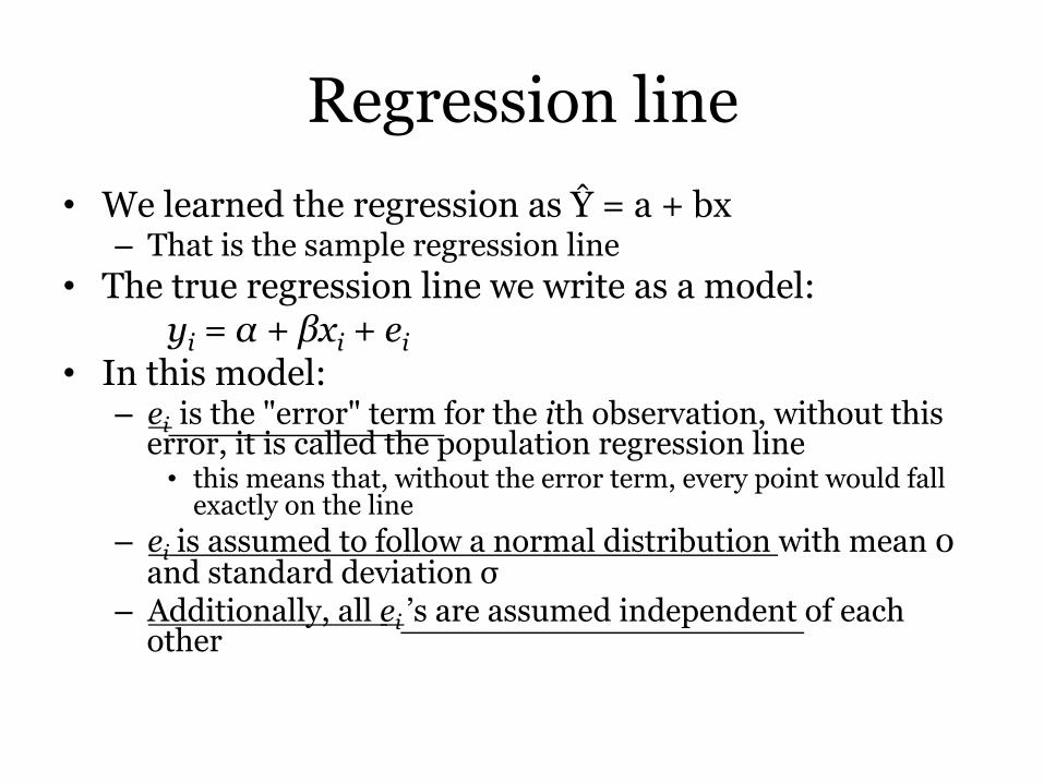
Regression line •  We learned the regression as Ŷ = a + bx

–  That is the sample regression line •  The true regression line we write as a model:

yi = α + βxi + ei •  In this model:

–  ei is the "error" term for the ith observation, without this error, it is called the population regression line

•  this means that, without the error term, every point would fall exactly on the line

–  ei is assumed to follow a normal distribution with mean 0 and standard deviation σ

–  Additionally, all ei ’s are assumed independent of each other

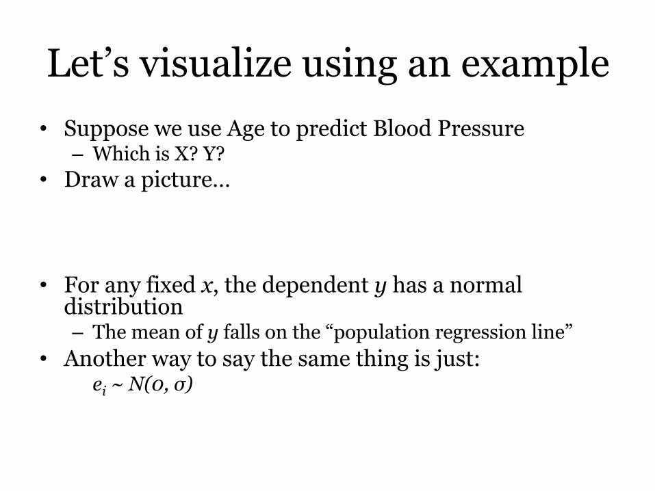
Let’s visualize using an example •  Suppose we use Age to predict Blood Pressure

–  Which is X? Y? •  Draw a picture…

•  For any fixed x, the dependent y has a normal distribution –  The mean of y falls on the “population regression line”

•  Another way to say the same thing is just: ei ~ N(0, σ)

Estimating the slope and intercept

•  Still apply the same formulas from Chapter 3 for the Least Squares estimates

•  The Least Squares method gives:

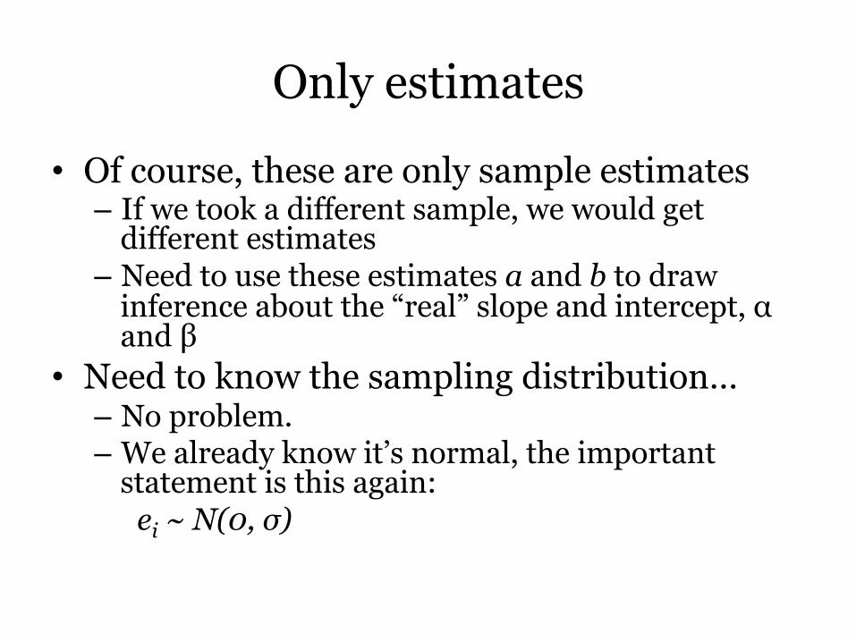
Only estimates

•  Of course, these are only sample estimates –  If we took a different sample, we would get

different estimates – Need to use these estimates a and b to draw

inference about the “real” slope and intercept, α and β

•  Need to know the sampling distribution… – No problem. – We already know it’s normal, the important

statement is this again: ei ~ N(0, σ)

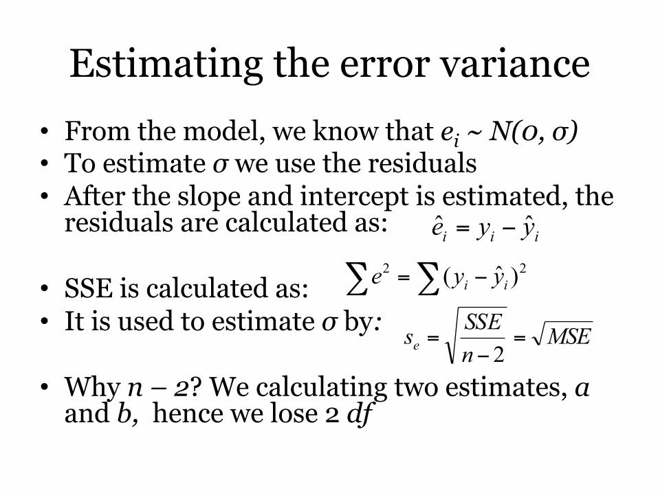
Estimating the error variance

•  From the model, we know that ei ~ N(0, σ) •  To estimate σ we use the residuals •  After the slope and intercept is estimated, the

residuals are calculated as:

•  SSE is calculated as: •  It is used to estimate σ by:

•  Why n – 2? We calculating two estimates, a and b, hence we lose 2 df

iii yye ˆˆ −=

∑∑ −= 22 )ˆ( ii yye

MSEnSSEse =−

=2

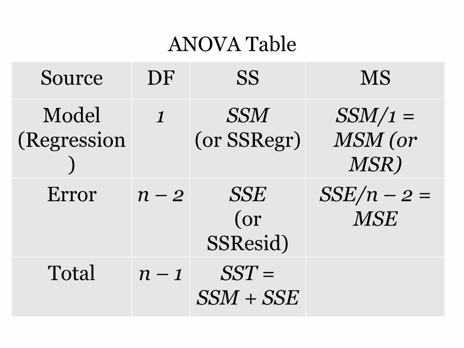
ANOVA Table

Source DF SS MS

Model (Regression

)

1 SSM (or SSRegr)

SSM/1 = MSM (or

MSR) Error n – 2 SSE

(or SSResid)

SSE/n – 2 = MSE

Total n – 1 SST = SSM + SSE

Sampling distribution of the slope, b

•  b follows a normal distribution – µb = β – σb = – So,

•  Replacing σb by sb gives us a familiar t distribution with df = n – 2

xxsσ

)1,0(~ N

s

bb

xx

bσβ

σβ −=

−

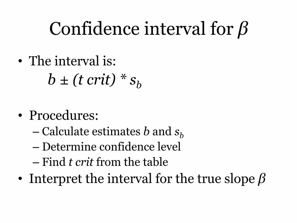
Confidence interval for β

•  The interval is: b ± (t crit) * sb

•  Procedures: – Calculate estimates b and sb – Determine confidence level – Find t crit from the table

•  Interpret the interval for the true slope β

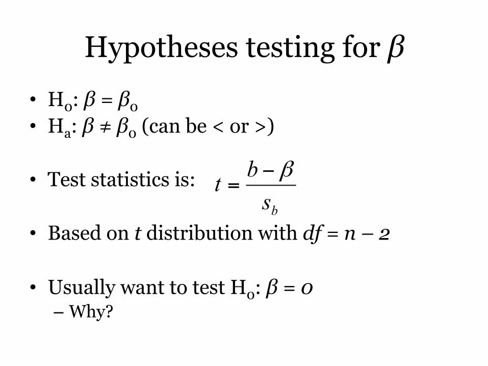
Hypotheses testing for β

•  H0: β = β0

•  Ha: β ≠ β0 (can be < or >)

•  Test statistics is: •  Based on t distribution with df = n – 2

•  Usually want to test H0: β = 0 – Why?

bsbt β−

=

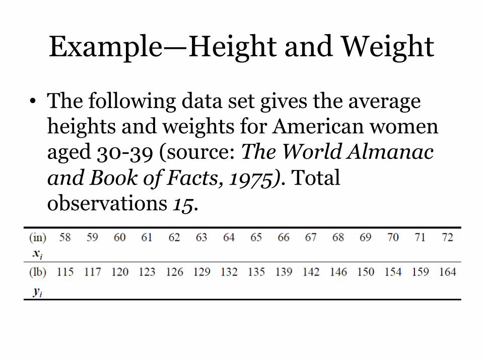
Example—Height and Weight

•  The following data set gives the average heights and weights for American women aged 30-39 (source: The World Almanac and Book of Facts, 1975). Total observations 15.

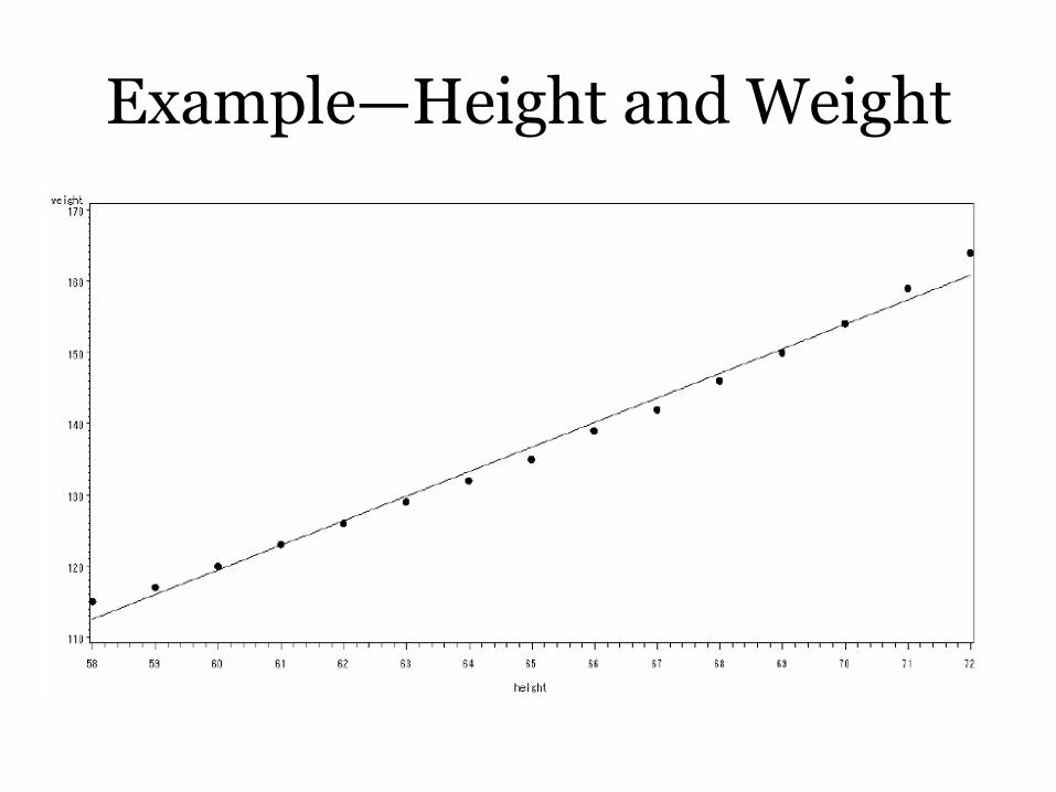
Example—Height and Weight

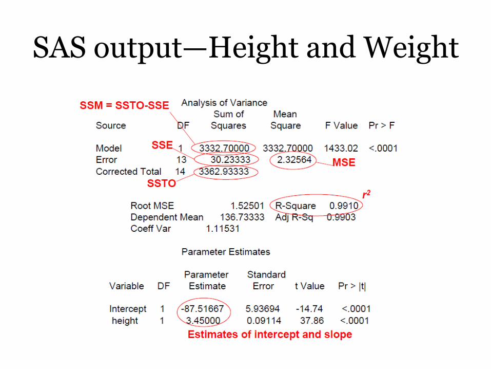
SAS output—Height and Weight

Using the SAS output for inference

•  Construct a 95% confidence interval for β

•  Test whether or not there is a significant linear relationship (H0: β = 0)

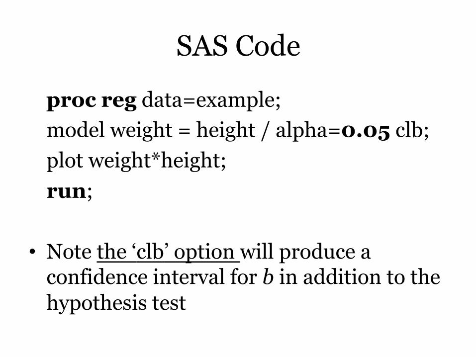
SAS Code

proc reg data=example; model weight = height / alpha=0.05 clb; plot weight*height; run;

•  Note the ‘clb’ option will produce a

confidence interval for b in addition to the hypothesis test

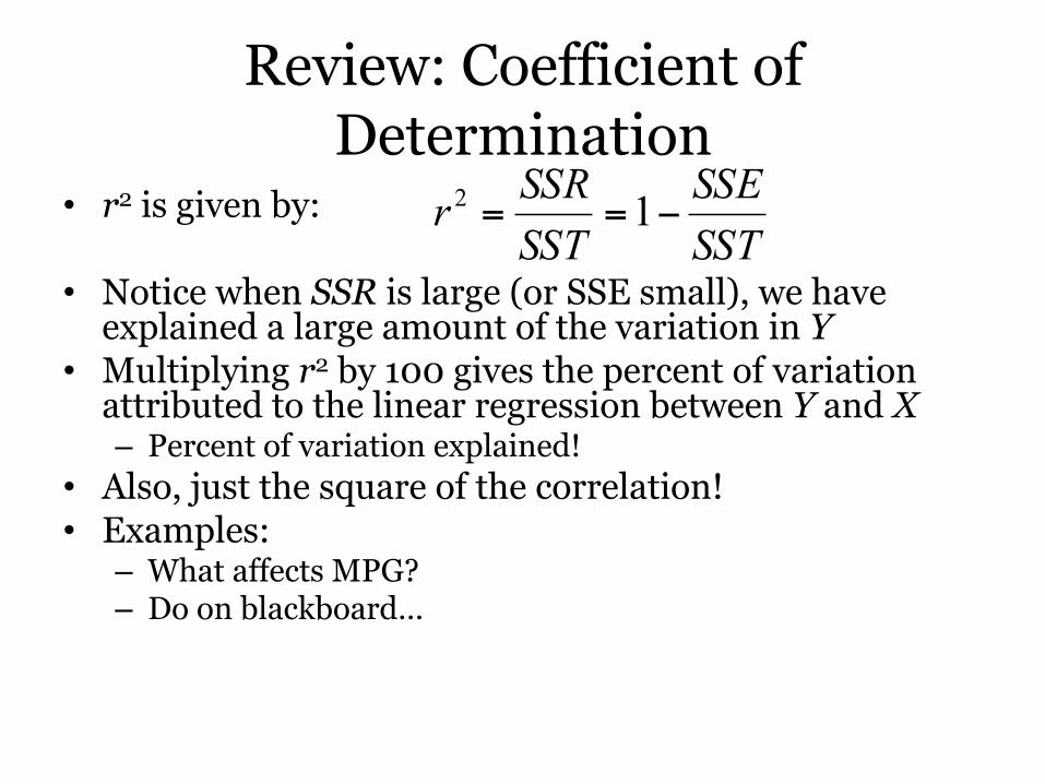
Review: Coefficient of Determination

•  r2 is given by:

•  Notice when SSR is large (or SSE small), we have explained a large amount of the variation in Y

•  Multiplying r2 by 100 gives the percent of variation attributed to the linear regression between Y and X –  Percent of variation explained!

•  Also, just the square of the correlation! •  Examples:

–  What affects MPG? –  Do on blackboard…

SSTSSE

SSTSSRr −== 12

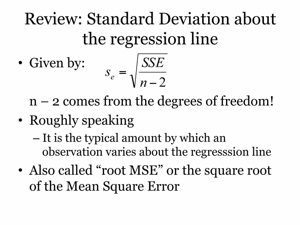
Review: Standard Deviation about the regression line

•  Given by:

n – 2 comes from the degrees of freedom! •  Roughly speaking

– It is the typical amount by which an observation varies about the regresssion line

•  Also called “root MSE” or the square root of the Mean Square Error

2−=nSSEse

SAS Code

proc reg data=example; model weight = height / alpha=0.05 clb;

àoutput out=fit r=res p=pred; plot weight*height;

run; •  This creates a new dataset called “fit” •  It contains:

–  ei, residuals in a variable called “res” –  , predicted values in a variable called “pred”

iy

Review: Residual Plots

•  The residuals can be used to assess the appropriateness of a linear regression model.

•  Specifically, a residual plot, plotting the residuals against x gives a good indication of whether the model is working – The residual plot should not have any pattern but

should show a random scattering of points –  If a pattern is observed, the linear regression

model is probably not appropriate.

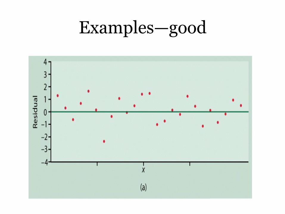
Examples—good

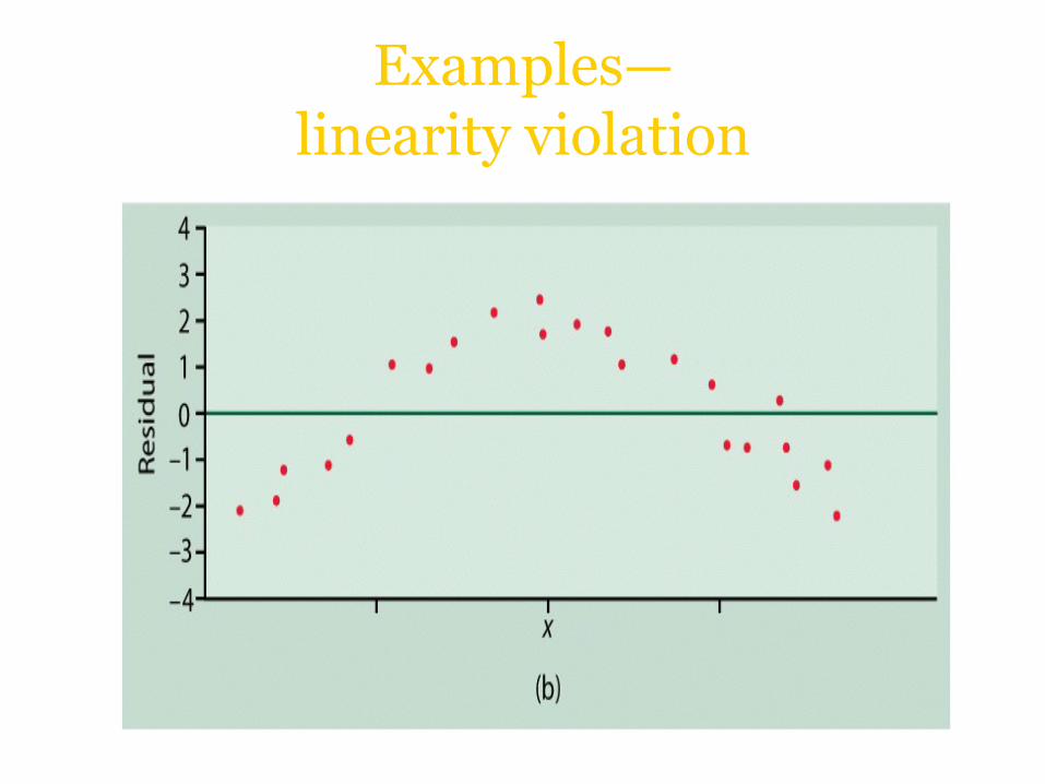
Examples— linearity violation

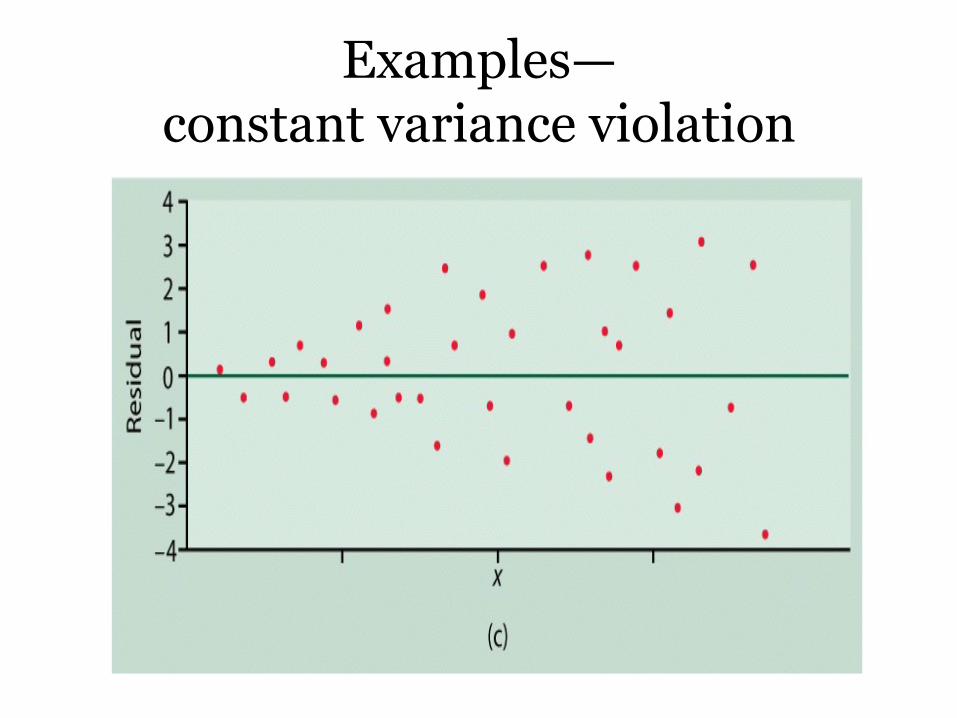
Examples— constant variance violation

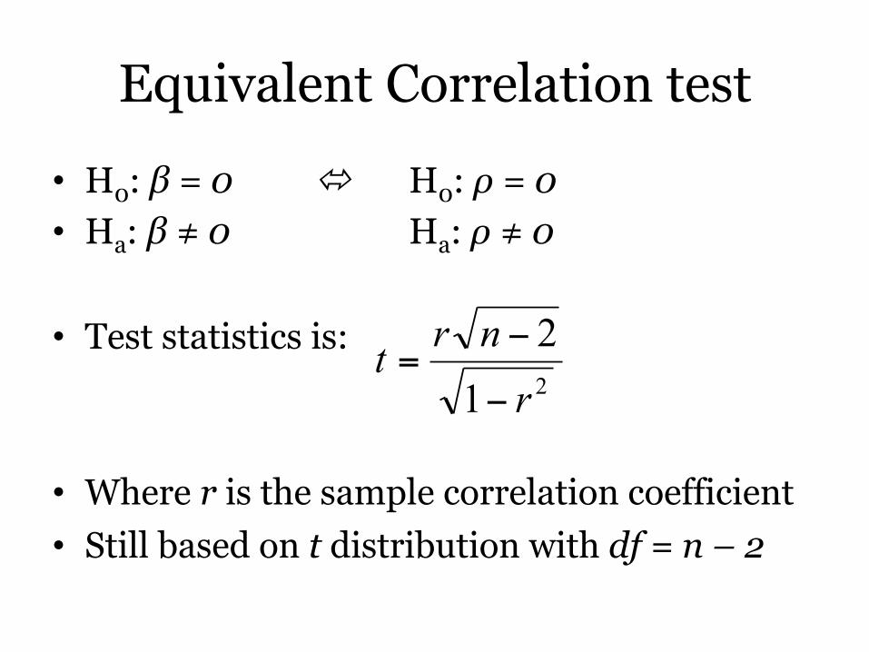
Equivalent Correlation test

•  H0: β = 0 ó H0: ρ = 0

•  Ha: β ≠ 0 Ha: ρ ≠ 0

•  Test statistics is:

•  Where r is the sample correlation coefficient •  Still based on t distribution with df = n – 2

212r

nrt−

−=

After Class… •  Read today’s Lecture Notes. •  Review Section 11.1 (optional part: “Exponential

Regression”) and 11.2 •  Read Section 11.4 for Monday’s Class.

•  Hw#10, due by Monday after next week. •  Lab #8, next Wed.

•  Make-up Exam for the Final –  If qualified, fill out the request form, no later than next

Friday, Apr 20th. –  Has to be taken before regular schedule. –  Make appointment with the testing center

4/16/12 Lecture 10 26

Multiple Regression Models

Chapter 11

Multiple Linear Regression

•  If we do include multiple Xs (or multiple X terms even), we call it Multiple Linear Regression or MLR

•  Most concepts are similar to Simple Linear Regression (SLR) with a single predictor – BUT… – Most things get a little more complicated also

•  Multiple “slopes” •  X’s can “mess up” each other

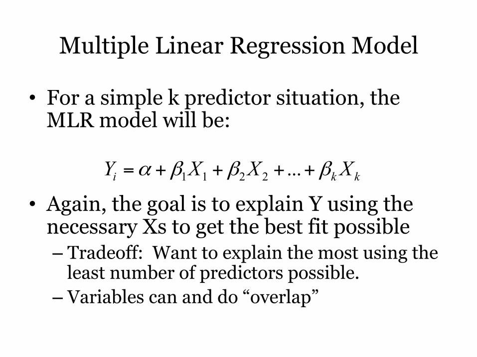
Multiple Linear Regression Model

•  For a simple k predictor situation, the MLR model will be:

•  Again, the goal is to explain Y using the necessary Xs to get the best fit possible – Tradeoff: Want to explain the most using the

least number of predictors possible. – Variables can and do “overlap”

kki XXXY βββα ++++= ...2211

A case study: •  We are interested in finding variables to predict college

GPA. •  Grades from high school will be used as potential

explanatory variables (also called predictors) namely: HSM (math grades), HSS (science grades), and HSE (english grades).

•  Since there are several explanatory variables or x’s, they need to be distinguished using subscripts:

– X1 =HSM – X2 =HSS – X3 =HSE

Several Simple Linear Regressions?

•  Why not do several Simple Linear Regressions –  Do GPA with HSM à Significant? –  Do GPA with HSS à Significant? –  Do GPA with HSE à Significant?

•  Why not? –  Each alone may not explain GPA very well at all but

used together they may explain GPA quite well. –  Predictors could (and usually do) overlap some, so

we’d like to distinguish this overlap (and remove it) if possible.

The scatterplots with the MLR line:

•  Unfortunately because scatterplots are restricted to only 2 axes (Y-axis and X-axis), they are less useful here.

•  Can plot Y with each predictor seperately, like an SLR, but this is just a preliminary look at each of the variables and cannot tell us whether we have a good MLR or not.

Interpretation of estimates

•  a is still the intercept

•  b1 is the estimated “slope” for β1, it explains how y changes as x1 changes – Suppose b1 = 0.7, then if I change x1 by 1 point,

y changes by 0.7, etc – The exact same interpretation as in SLR

•  Then what about b2? b3?

Other things that are the same •  Predicted values

– Given values for x1, x2, and x3, plug those into the regression equation and get a predicted value

•  Residuals – Still Observed – Predicted = y – y_hat – Calculations and interpretations are the same

•  Assumptions – Independence, Linearity, Constant Variance

and Normality – Use the same plots, same interpretation

More things that are the same*

•  Confidence intervals for the slopes – Still of the form b ± (t crit)sb – *CHANGE!!!

•  DF = n – p – 1 •  p is the number of predictors in our model •  Recall in SLR we only had 1 predictor, or one x

–  So, df = n – 1 – 1 = n – 2 for SLR

•  Now we have p predictors, •  For GPA example, df = n – 3 – 1 = n – 4

Now the changes…

•  Since there is more than 1 predictor, a simple t-test will not suffice to test whether there is a significant linear relationship or not.

•  The good news… – The fundamental principle is still the same – To help with understanding let’s look at what

R-square means…

Recall: R-square

•  Still trying to explain the changes in Y •  R-square measures the % of explained

variation by the regression line. – So in SLR, this is just the percent explained by

the changes in x. – In MLR, it represents the percent explained by

all predictors combined simultaneously. •  Problem: What if the predictors are overlapping?

In fact, they almost always overlap at least a little bit

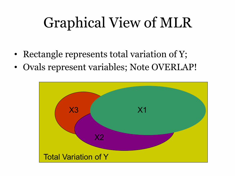
Graphical View of MLR

•  Rectangle represents total variation of Y; •  Ovals represent variables; Note OVERLAP!

X1

X2

X3

Total Variation of Y

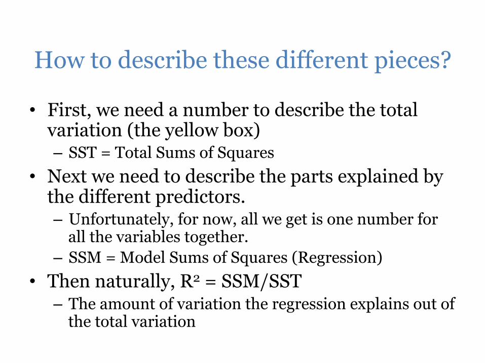
How to describe these different pieces?

•  First, we need a number to describe the total variation (the yellow box) –  SST = Total Sums of Squares

•  Next we need to describe the parts explained by the different predictors. –  Unfortunately, for now, all we get is one number for

all the variables together. –  SSM = Model Sums of Squares (Regression)

•  Then naturally, R2 = SSM/SST –  The amount of variation the regression explains out of

the total variation

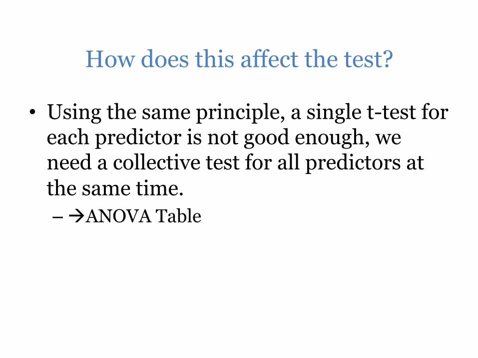
How does this affect the test?

•  Using the same principle, a single t-test for each predictor is not good enough, we need a collective test for all predictors at the same time. – àANOVA Table

Figure 11.4 Introduction to the Practice of Statistics, Sixth Edition © 2009 W.H. Freeman and Company

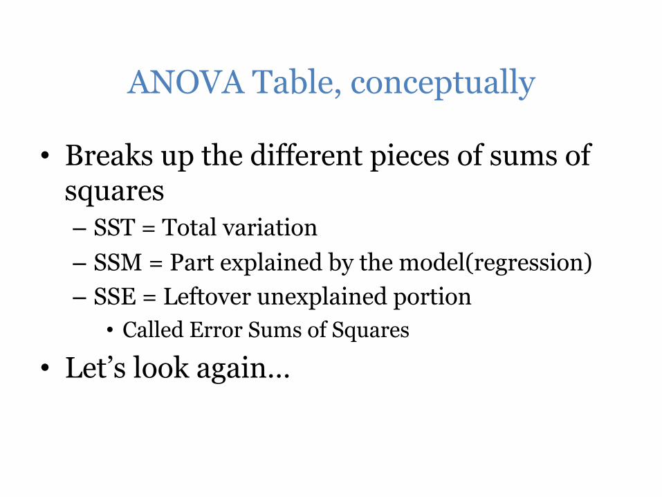
ANOVA Table, conceptually

•  Breaks up the different pieces of sums of squares –  SST = Total variation –  SSM = Part explained by the model(regression) –  SSE = Leftover unexplained portion

•  Called Error Sums of Squares

•  Let’s look again…

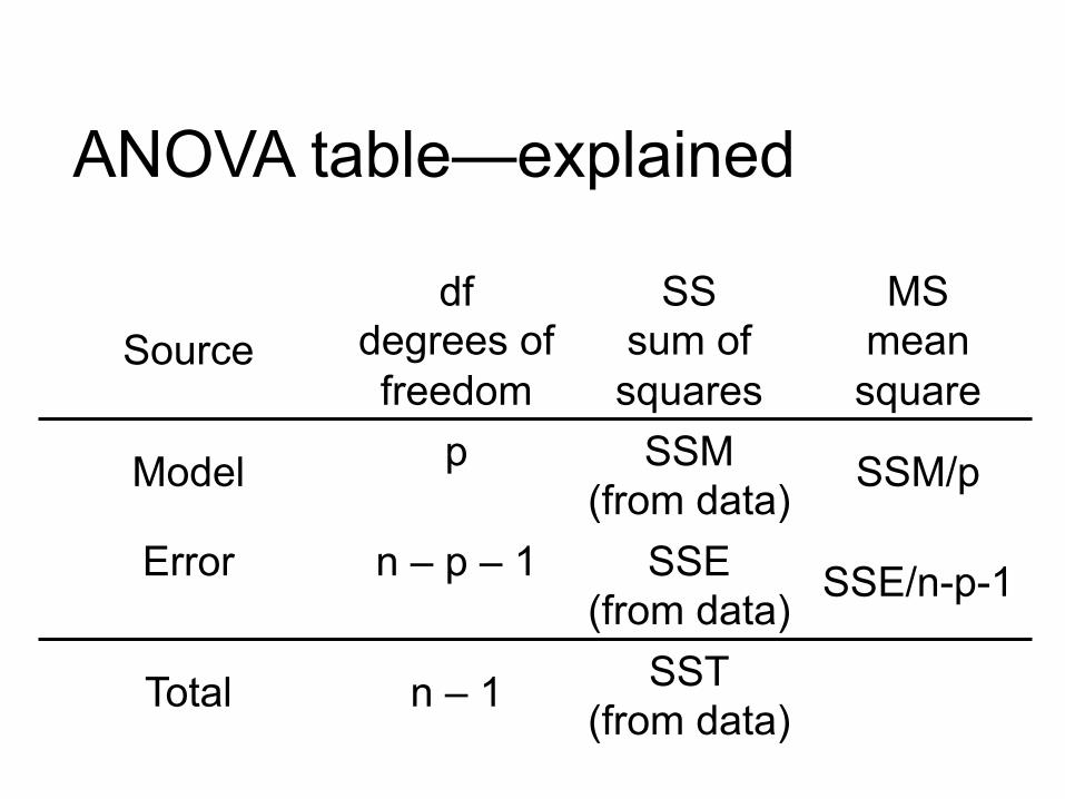
Source

df degrees of freedom

SS sum of

squares

MS mean

square

Model p SSM (from data)

SSM/p

Error n – p – 1 SSE (from data)

SSE/n-p-1

Total

n – 1 SST (from data)

ANOVA table—explained

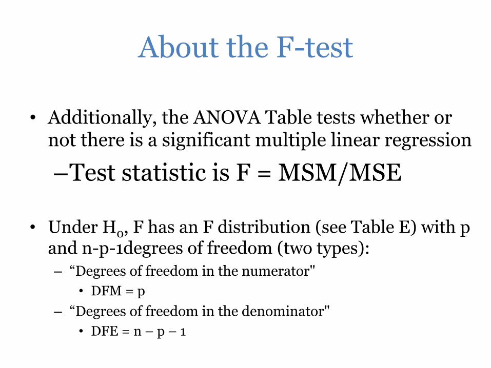
About the F-test

•  Additionally, the ANOVA Table tests whether or not there is a significant multiple linear regression

– Test statistic is F = MSM/MSE

•  Under H0, F has an F distribution (see Table E) with p and n-p-1degrees of freedom (two types): –  “Degrees of freedom in the numerator"

•  DFM = p –  “Degrees of freedom in the denominator"

•  DFE = n – p – 1

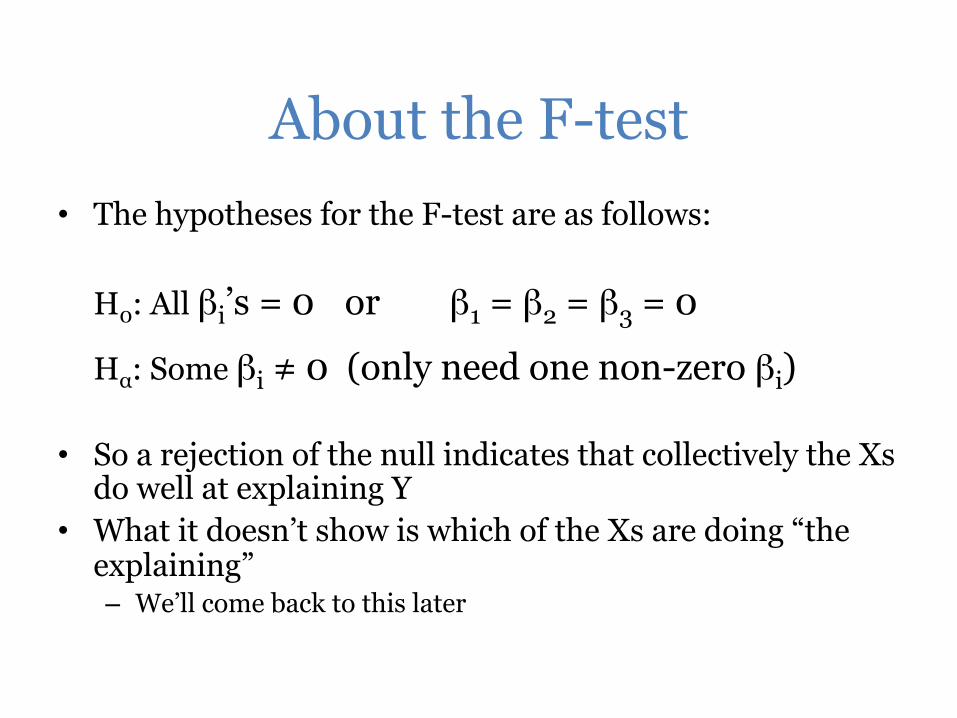
About the F-test •  The hypotheses for the F-test are as follows:

H0: All βi’s = 0 or β1 = β2 = β3 = 0

Hα: Some βi ≠ 0 (only need one non-zero βi) •  So a rejection of the null indicates that collectively the Xs

do well at explaining Y •  What it doesn’t show is which of the Xs are doing “the

explaining” –  We’ll come back to this later

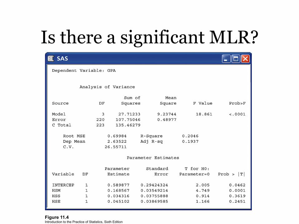
Figure 11.4 Introduction to the Practice of Statistics, Sixth Edition © 2009 W.H. Freeman and Company

Is there a significant MLR?

Conclusion?

•  Since the P-value for the F-test is small, <0.0001, we reject H0, there is a significant Multiple Linear Regression between Y and the Xs.

•  Model is useful in predicting Y •  Can you explain it in plain language?

Which X’s are actually explaining Y?

•  The t-tests now become useful in determining which predictors are actually contributing to the explanation of Y.

•  There are several different methods of determining which Xs are the best –  All possible models selection –  Forward selection –  Stepwise selection –  Backward elimination

•  We will just learn backward elimination…