indonesian highway capacity manual - … · indonesian highway capacity manual urban and semi-urban...
TRANSCRIPT

INDONESIAN
HIGHWAY CAPACITY MANUAL
PART - I URBAN ROADS
NO. 09/T/BNKT/ 1993
DIRECTORATE GENERAL OF HIGHWAYSMINISTRY OF PUBLIC WORKS

INDONESIAN HIGHWAY CAPACITY MANUAL
URBAN AND SEMI-URBAN TRAFFIC FACILITIES
JANUARY 1993
FOREWORD
Chapter 1: INTRODUCTION
Chapter 2: SIGNALISED INTERSECTIONS
Chapter 3: UNSIGNALISED INTERSECTIONS
Chapter 4: WEAVING SECTIONS
Chapter 5: URBAN ROADS

INDONESIAN HIGHWAY CAPACITY MANUAL
TABLE OF CONTENTS
FOREWORD
CHAPTER 1 INTRODUCTION ................................................................................. 1 – 1
1. BACKGROUND ..................................................................................................... 1 – 12. SCOPE AND OBJECTIVES .................................................................................... 1 – 14. GENERAL DEFINITIONS AND TERMINOLOGY ................................................. 1 – 45. USER GUIDELINES ............................................................................................... 1 – 66. GENERAL LITERATURE REFERENCES ............................................................... 1 – 8
CHAPTER 2 SIGNALISED INTERSECTIONS ......................................................... 2 – 1
1. INTRODUCTION ................................................................................................... 2 – 21.1 Scope and objectives ..................................................................................... 2 – 21.2 Characteristics of traffic signals .................................................................... 2 – 21.3 Definitions and terminology ......................................................................... 2 – 6
2. METHODOLOGY .................................................................................................. 2 – 10 2.1 General principles ......................................................................................... 2 – 10
2.2 Overview of the calculation procedure ......................................................... 2 – 18 2.3 Guidelines for application ............................................................................ 2 – 193. CALCULATION PROCEDURE ............................................................................. 2 – 234. WORKED EXAMPLES ........................................................................................... 2 – 535. LITERATURE REFERENCES ................................................................................. 2 – 75
Appendix 2:1 Calculation forms ......................................................................................... 2 – 76
CHAPTER 3 UNSIGNALISED INTERSECTIONS ................................................... 3 – 1
1. INTRODUCTION ................................................................................................... 3 – 21.1 Scope and objectives .................................................................................... 3 – 21.2 Definitions and terminology ......................................................................... 3 – 3
2. METHODOLOGY .................................................................................................. 3 – 93. CALCULATION PROCEDURE ............................................................................. 3 – 134. WORKED EXAMPLES ........................................................................................... 3 – 325. LITERATURE REFERENCES ................................................................................. 3 – 38
Appendix 3:1 Calculation forms ........................................................................................ 3 – 39
I

CHAPTER 4 WEAVING SECTIONS ..................................................................... 4 – 1
1. INTRODUCTION ................................................................................................ 4 – 2 1.1 Scope and objectives ........................................................................................ 4 – 2 1.2 Definitions and terminology ............................................................................ 4 – 32. METHODOLOGY ................................................................................................ 4 – 83. CALCULATION PROCEDURE .......................................................................... 4 – 124. WORKED EXAMPLES ......................................................................................... 4 – 325. LITERATURE REFERENCES ................................................................................ 4 – 43
Appendix 4:1 Calculation forms .....................................................................: ..................... 4 – 45
CHAPTER 5 URBAN ROADS ................................................................................. 5 – 1
1. INTRODUCTION ................................................................................................. 5 – 3 1.1 Scope and objectives ........................................................................................ 5 – 3 1.2 Road characteristics .......................................................................................... 5 – 5
1.3 Definitions and terminology ............................................................................ 5 – 72. METHODOLOGY ................................................................................................ 5 – 143. CALCULATION PROCEDURE FOR URBAN ROADS .................................... 5 – 224. CALCULATION PROCEDURE FOR URBAN MOTORWAYS ...................... 5 – 455. WORKED EXAMPLES ......................................................................................... 5 – 546. LITERATURE REFERENCES ................................................................................ 5 – 83
Appendix 5:1 Calculation forms ............................................................................................ 5 – 85
CHAPTER 6 INTERURBAN ROADS (To be produced in HCM Phase2)
CHAPTER 7 MOTORWAYS (To be produced in HCM Phase 2)
II

FOREWORD

FOREWORD
Planning, design and operational analysis for Indonesian highway traffic facilities have so far mainly been based on foreign capacity models, guidelines and standards. However, since 1982, some studieson Highway Traffic Engineering in Indonesia had shown that directapplication of models and methods based on western traffic characteristics (e.g. speed-flow relationships, saturation flows, capacity) to situations in Indonesia often produced misleading results. Two main reasons for this were identified that :
(1) The traffic composition in Indonesia includes a high ratio of motorcycles and unmotorised vehicles.
(2) No right of way rules are applied at intersections and other conflict points.
The need for an Indonesian Highway Capacity Manual was thus identified in 1986 by a joint committee of Directorate General of Bina Marga, Indonesian Road Engineering, and the S2-STJR-ITB Programme.Phase 1 Indonesian Highway Capacity Manual study was started in December 1990 and the main task was Development of a HighwayCapacity Manual for different types of traffic facilities in urban and semi urban environments.
The Directorate General of Bina Marga has introduced a "standardization" policy which endeavors to optimize investments, designs and construction methods for highways so as to obtain the most efficient use of available resources, finances and materials, as well as improvement of the ability of local engineers and contractors.
For this purpose, standard guidance regarding Methods Specifications, Testing Material and other aspects of Planning, Design, Construction, Operation and Maintenance have a high level of necessity in achieving a more efficient use of road facilities.This book entitled "Indonesian Highway Capacity Manual" for Urban Roads is part of the efforts of the Directorate General of Bina Marga in promoting professionalism for everyone involved in road development.

A large number of government agencies all over Indonesia have given very valuable assistance to the Development of the Manual.Directorate General of Bina Marga hereby expresses a sincere gratitude to all those who have contributed to this first version of the Indonesian Highway Capacity Manual.
As we realize that there is room for further improvement of thismanual, especially considering Indonesian road traffic conditions,any comments and suggestions will be most welcome.
Jakarta, January 1993
Director of Urban Road Development
Sunaryo Sumadji
STEERING COMMITTEE
INDONESIAN HIGHWAY CAPACITY MANUAL
PHASE I - URBAN ROADS
Chairman :
Ir. Djoko Asmoro Dit. Binkot (Dec 1990 – Sept 1991)Ir. Subagya Sastrosoegito Dit. Binkot (Sept 1991 – Nov 1992)Ir. Sunaryo Sumadji Dit. Binkot (Nov 1992 - Jan 1993)
Secretary :
Ir. Sukawan Mertasudira M.Sc Dit. Binkot
Project Officer :
Ir. Palgunadi M.Eng.Sc Dit. Binkot
Other committee members :
Brigjen (Pol) Drs. Sony H. Dit. Lantas Polri Prof. Ir. T. Soegondo MSCE ITB S2 STJR Ir. Iskandar Abubakar M.Sc Dit. Jen. Perhubungan DaratIr. Hasan Basri Saleh M.Sc Dit. Jen. Perhubungan DaratIr. Gandhi Harahap M.Eng Puslitbang JalanDR. Ir. Hermanto Dardak M.Eng.Sc Puslitbang JalanIr. Moh. Anas Aly Dit. BipranDrs. Muchsin Asegaaf Dit. BipranIr. Muksin M.Eng.Sc Dit. Binkot Ir. Trihardjo Dit. BinkotIr. Janeydi Juni Dit. Binkot

Chapter 1: INTRODUCTION

HCM: INTRODUCTION
CHAPTER 1
INTRODUCTION
1. BACKGROUND
Highway Capacity Manuals are necessary tools for proper planning, design and operation of road traffic facilities. The fundamental traffic characteristics knowledge contained in suchmanuals are also an essential input in models for cost-efficient management of road systems, trafficforecasting and assignment with capacity restraint. Highway administrations in manydeveloped countries therefore devote considerable resources to the production of suchmanuals and guidelines appropriate to their own, conditions.
The main hypothesis behind the project that has resulted in this manual is that Indonesian traffic characteristics are fundamentally different from those in developed countries. Existing capacity manuals from such countries therefore cannot be successfully imple-mented in Indonesia. The aim of the research behind the production of this manual has been to explore and model Indonesian driver behaviour and fundamental road traffic characteristicsby means of extensive field data collection and analysis.
The data collection was performed by the Consultants between May and December 1991. Table 1:1presents the distribution of field data collection sites on different types of traffic facilitiesand cities. A total of 147 sites in 16 cities all over Indonesia were surveyed as shown inthe table. At each site a continuous video recording of all traffic movements in the facilityfrom early morning to late afternoon was obtained for data reduction and analysis in theHCM project laboratory in Bandung.
2. SCOPE AND OBJE CTIVES
The scope of this first, interim edition of the Indonesian Highway Capacity Manual is restricted to traffic facilities in urban and semi-urban areas, with chapters covering differenttypes of interurban roads to be added in the spring of 1994 as a result of the secondphase of the HCM project. A comprehensive edition of the manual, including trafficengineering guidelines and computer software, will be produced in Bahasa Indonesia in thethird and final HCM project phase 1995.
The types of facilities covered, and the traffic effects that can be calculated with the use of thepresent manual are recorded in Table 2:1 below.
1 - 1

HCM: INTRODUCTION
No. of surveyed sites
No City Signalisedintersection
UnsignalizedIntersection
WeavingSections Road links Total
1 Bandung 20 9 5 17 512 Jakarta 8 6 12 6 32
Cianjur 1 0 0 0 1Sukabumi 1 2 0 1 4
3 Tasikmalaya 1 1 0 0 2yogyakarta 2 1 0 1 4Semarang 2 0 3 0 5
4 Surabaya 2 3 3 2 10Malang 3 0 0 0 3Denpasar 2 2 0 1 5kupang 2 1 0 0 3
5 Ujung Pandang 2 2 2 2 8Ambon 2 3 0 1 4
6 Palembang 0 1 0 1 4Medan 2 2 2 2 8Pontianak 2 0 0 1 3
52 33 27 35 147
Table 1:1 Field data collection in urban and semi-urban areas during HCMproject Phase 1.
The manual can also be used to analyse routes or networks within urban areas by means of successive aplication of the relevant chapter for each traffic facility. The total travel time can then be obtained as the sum of the travel times and delays in each link and node along the studied route.
1 - 2
HCM: INTRODUCTION
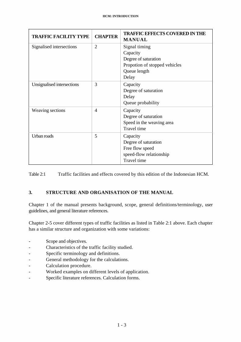
TRAFFIC FACILITY TYPE CHAPTER TRAFFIC EFFECTS COVERED IN THE MANUAL
Signalised intersections 2 Signal timingCapacityDegree of saturation Propotion of stopped vehicles Queue lengthDelay
Unsignalised intersections 3 CapacityDegree of saturation DelayQueue probability
Weaving sections 4 CapacityDegree of saturationSpeed in the weaving area Travel time
Urban roads 5 CapacityDegree of saturation Free flow speed speed-flow relationship Travel time
Table 2:1 Traffic facilities and effects covered by this edition of the Indonesian HCM.
3. STRUCTURE AND ORGANISATION OF THE MANUAL
Chapter 1 of the manual presents background, scope, general definitions/terminology, userguidelines, and general literature references.
Chapter 2-5 cover different types of traffic facilities as listed in Table 2:1 above. Each chapterhas a similar structure and organization with some variations:
- Scope and objectives. - Characteristics of the traffic facility studied.- Specific terminology and definitions. - General methodology for the calculations. - Calculation procedure.- Worked examples on different levels of application. - Specific literature references. Calculation forms.
1 - 3

HCM: INTRODUCTION
4. GENERAL DEFINITIONS AND TERMINOLOGY
notations, terminology and definitions of conditions and characteristics of a more general nature are presented below. Definitions of more specific nature are presented in Chapters2 – 5 for each type of traffic facility.
TRAFFIC CONDITIONS AND CHARACTERISTICS
TRAFFIC ELEMENT Object or pedestrian being part of traffic
Veh VEHICLE Traffic element on wheels
LV LIGHT VEHICLE Index for motor vehicle on four wheels (including passenger car, oplet, micro bus, pick-up and microtruck according to Bina Marga classificationssystem)
HV HEAVY VEHICLE Index for motor vehicle with two or three wheels (including bus, 2-axle truck, 3-axle truck and truckcombinations according to Bina Margaclassifications system).
MC MOTOR CYCLE Index for motor vehicle with two or three wheels(including motor cycle and 3-wheeled vehicleaccording to Bina Marga classifications system).
UM UNMOTORISED Index for unmotorised traffic element on wheels(including becak, bicycles, horse-carriage andpushcarts according to Bina Marga classificationssystem).
P RATIO Ratio of a sub-population to the total populations,e.g. PMC = ratio of motorcycles in the traffic flow.
pcu PASSENGER CAR UNIT Conversion factor for different vehicle types withregard to their impact on capacity as compared to a passenger car(i.e. for passenger cars and otherlight vehicle pcu = 1.0)
Q TRAFFIC FLOW Number of traffic elements passing a point on a road per unit of time (e.g. veh/h; pcu/h).
PHF PEAK HOUR FACTOR Ratio between the peak hour flow and four timesthe highest quarterly flow during the same hour.
1 - 4

HCM: INTRODUCTION
LEVEL OF PERFORMANCE MEASURES
LoP LEVEL OFPERFORMANCE
Quantitative measure describing the operationalconditions of a traffic facility as perceived by the highway authority (generally described in terms of capacity, degree of saturation, average speed, travel time, delay, queue probability, queue length, ratio of stopped vehicles).
LoS LEVEL OF SERVICE Qualitative measure describing the operationalconditions within a traffic stream and theirperception by highway users (generally described in terms of speed, travel time,freedom to maneuver, traffic interruptions,comfort, convenience, safety).
C CAPACITY Maximum sustainable traffic flow at a road section during given conditions (e.g geometricdesign, environment, traffic composition etc.Normally expressed in veh / h or pcu / h).
Co BASE CAPACITY Capacity of a road section with a predeterminedset of (ideal) conditions.
DS DEGREE OFSATURATION
Ratio of flow to capacity.
V SPEED Vehicle speed (normally space-mean speedkm/h or m /sec).
V0 FREE FLOW SPEED Desired vehicle speed at traffic flow = 0.
HOUR Time unit.
min MINUTE Time unit
sec SECOND Time unit
T TIME Time
TT TRAVEL TIME Time difference between passage of start and end point of an un-interrupted journey.
D DELAY Extra travel time required to pass anintersection as compared to a situation withoutthe intersection.
PSV PROPORTION OF STOPPED VEHICLES
Ratio of flow forced to come to a completestandstill.
QP% QUEUE PROBABILITY Probability of queue with more than twovehicles in any approach to an unsignalisedintersection.
1 - 5

HCM: INTRODUCTION
GEOMETRIC CONDITIONS AND CHARACTERISTICS
L LENGTH Length of a road segment
W WIDTH Width of a road section
GRAD GRADIENT Gradient of a road segment in the direction of travel (+/-%).
APPROACH Area for entering vehicle in a traffic facility.
MEDIAN Area separeting traffic directions on a road segment
ENVIRONMENT CONDITIONS
COM COMMERCIAL Commercial landuse (e.g. shops, restaurants, offices) with direct roadside acces for pedestrians and vehicle
RES RESIDENTIAL Residential landuse with direct roadside acces forpedestrians and vehicles.
RA RESTRICTED ACCES No or limited direct roadside acces (e.g due to the existence of physical barriers, frontage streets etc).
CS CITY SIZE Number of inhabitants in an urban area
SF SIDE FRICTION Interaction between traffic flow and roadsideactivities causing a reduction of capacity and speed.
5. USER GUIDELINES
This Highway Capacity manual should be used as atool in planning, design and operational analysis of all highway traffic facilities. The user of the manual will thus include tansportation planners, traffic engineers and highway engineers in transport and highway administrations as well as in consulting companies.
The manual is designed to allow the user to predict the level of performance of a traffic facility for a given set of traffic, geometric and environmental conditions. Default values are proposed for use in cases when some required input data is missing.
By succesive calculations with adjusted input data, the geometric design which gives a desired level of performance for given traffic flow and environmental conditions can be determined. In the same way, the rate of decline of level of performance at a given traffic
1 - 6

HCM: INTRODUCTION
facility as a result of. traffic growth can be analysed, and the timing of the need. for capacity expansion determined.
Many other questions relevant to a traffic or highway engineer can be answered by the sametype of "trial-an-error" calculations with different sets of input data. The manual canthus be used in variety of situations as exemplified below:
a) PlanningDetermination of suitable layout and preliminary design of a new traffic facility based on forecasted traffic flows.
b) DesignDetermination of suitable detailed geometric design and traffic control parameters for a new or revised traffic facility with known traffic flow.
c) Operational analysisDetermination of the level of performance of 'an existing traffic facility. Determination ofsignal timing for minimum delay. Prediction of the consequences of minorchanges in geometry, traffic regulations and signal control.
The manual also enables calculation of the level of performance of the facility at a given traffic demand. Development of traffic engineering guidelines, and recommendations regarding threshold values for design and operation, will be undertakenin phase 3 of the HCM project for incorporation in the final version of the manual.
Standard forms are provided for each type of traffic facility for recording of input data as well as for the different calculation steps. The worked examples which have been included at the end of each traffic facility chapter also give useful guidance concerning ways to applythe manual.
Although the manual is designed for a wide range of conditions, it is advisable for the readerto make his own critical evaluation of the results and to supplement them with own fieldmeasurements of capacity and other measures of performance whenever possible.
Comments about possible errors in the manual and suggestions for improvements and further development are very much appreciated. These could be addressed to Binkot, Bina Marga or to the HCM project office in Bandung.
1 - 7
HCM: INTRODUCTION
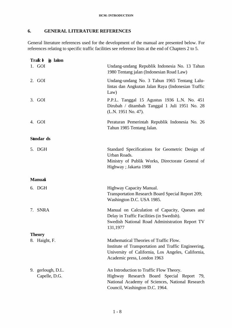
6. GENERAL LITERATURE REFERENCES
General literature references used for the development of the manual are presented below. For references relating to specific traffic facilities see reference lists at the end of Chapters 2 to 5.
Traffic le gis lation1. GOI Undang-undang Republik Indonesia No. 13 Tahun
1980 Tentang jalan (Indonesian Road Law)
2. GOI Undang-undang No. 3 Tahun 1965 Tentang Lalu-lintas dan Angkutan Jalan Raya (Indonesian TrafficLaw)
3. GOI P.P.L. Tanggal 15 Agustus 1936 L.N. No. 451 Dirubah / ditambah Tanggal 1 Juli 1951 No. 28 (L.N. 1951 No. 47).
4. GOI Peraturan Pemerintah Republik Indonesia No. 26 Tahun 1985 Tentang Jalan.
Standar ds
5. DGH Standard Specifications for Geometric Design of Urban Roads.Ministry of Publik Works, Directorate General of Highway ; Jakarta 1988
Manuals
6. DGH Highway Capacity Manual.Transportation Research Board Special Report 209; Washington D.C. USA 1985.
7. SNRA Manual on Calculation of Capacity, Queues and Delay in Traffic Facilities (in Swedish). Swedish National Road Administration Report TV 131,1977
Theory8. Haight, F. Mathematical Theories of Traffic Flow.
Institute of Transportation and Traffic Engineering, University of California, Los Angeles, California,Academic press, London 1963
9. gerlough, D.L. Capelle, D.G.
An Introduction to Traffic Flow Theory.Highway Research Board Special Report 79, National Academy of Sciences, National ResearchCouncil, Washington D.C. 1964.
1 - 8
Chapter 2: SIGNALISED INTERSECTIONS

IHCM: SIGNALISED INTERSECTIONS
CHAPTER 2 SIGNALISED INTERSECTIONS
TABLE OF CONTENTS
1. INTRODUCTION .............................................................................................2 – 2
1.1 SCOPE AND OBJECTIVES ......................................................................2 – 2 1.2 CHARACTERISTICS OF TRAFFIC SIGNALS .....................................2 – 2
1.3 DEFINITIONS AND TERMINOLOGY .................................................2 – 6
2. METHODOLOGY .............................................................................................2 – 10
2.1 GENERAL PRINCIPLES .........................................................................2 – 102.2 OVERVIEW OF THE CALCULATION PROCEDURE .......................2 – 182.3 GUIDELINES FOR APPLICATION ........................................................2 – 19
2.3.1 Types of application of the manual ...............................................2 – 192.3.2 Default values ..................................................................................2 – 20
3. CALCULATION PROCEDURE ......................................................................2 – 23
STEP A: INPUT DATA ..............................................................................2 – 24A-1: Geometric/ traffic control and
environmental conditions ..............................................2 – 24A-2: Traffic flow conditions ..................................................2 – 26
STEP B: SIGNALISATION ......................................................................2 – 27B-1: Signal phasing .................................................................2 – 27B-2: Clearance time and lost time .......................................2 – 28
STEP C: SIGNAL TIMING ......................................................................2 – 30C-1: Approach type ................................................................2 – 30C-2: Effective approach width ...............................................2 – 32
C-3: Base saturation flow ........................................................2 – 33C-4: Correction factors ...........................................................2 – 37C-5: Flow/saturation flow ratio ............................................2 – 41C-6: Cycle time and green times ..........................................2 – 42
STEP D: CAPACITY ..................................................................................2 – 44D-1: Capacity ...........................................................................2 – 44D-2: Need for revisions ...........................................................2 – 45
STEP E: LEVEL OF PERFORMANCE ....................................................2 – 46E-1: Preparations ....................................................................2 – 46E-2: Queue length ..................................................................2 – 47
E-3: Stopped vehicles .............................................................2 – 49E-4: Delay ................................................................................2 – 50
4. WORKED EXAMPLES .....................................................................................2 – 53
5. LITERATURE REFERENCES ......................................................................2 – 75
APPENDIX 2:1 Calculation forms ...........................................................2 – 76
2 - 1

IHCM: SIGNALISED INTERSECTIONS
1 . INTRODUCTION
1.1 SCOPE AND OBJECTIVES
This chapter describes procedures for determination of signal timing, capacity and level of performance (delay, queue length and proportion of stopped vehicles) for signalisedintersections in urban and semi-urban areas.
The manual primarily deals with isolated, fixed-time controlled signalised intersections(definitions see Section 1.3 below) with normal geometric layout (four-arm and three-arm)and traffic signal control devices. It can with some considerations also be used for analysis ofother geometric layouts.
Signalised intersections which are part of a coordinated, fixed time control system, or isolated vehicle actuated traffic signals, can also be analysed with the help of the manual, see Section2.3:1. Only very few such systems were however operational in Indonesia at the time of the preparation of the manual.
Normally traffic signals are introduced for one or more of the following reasons:
- to avoid blockage of an intersection by conflicting traffic streams, thus guaranteeingthat a certain capacity can be maintained even during peak traffic conditions;
- to facilitate the crossing of a major road by vehicles and/or pedestrians from a minorroad;
- to reduce the number of traffic accidents caused by collisions between vehicles inconflicting directions.
Signalisation does not always increase the capacity and safety of an intersection. By application of the methods described in this and other chapters in the manual it is howeverpossible to estimate the effect of signalisation on capacity and level of performance as compared to unsignalised control or round-about control.
1.2 CHARACTERISTICS OF TRAFFIC SIGNALS
For most types of traffic facilities capacity and level of performance is primarily a function ofgeometric conditions and traffic demand. By means of the signals however, the plan-ner/engineer can distribute capacity to different approaches through the green time allocatedto each approach. In order to calculate capacity and level of performance it is therefore necessary to first determine the signal phasing and timing which is most appropriate for the studied conditions.
Signalisation by means of three-coloured lights (green, amber, red) is applied to separate passage of conflicting traffic movements in time. This is an absolute requirement for trafficmovements arriving from intersecting streets = primary conflicts. The signals can also be used to separate turning movements from opposing straight-through traffic, or to separate turning traffic from crossing pedestrians = secondary conflicts, see Figure 1.2:1 below.
2 - 2

IHCM: SIGNALISED INTERSECTIONS
Figure 1.2:1 Primary and secondary conflicts in a four-arm, signalised intersection.
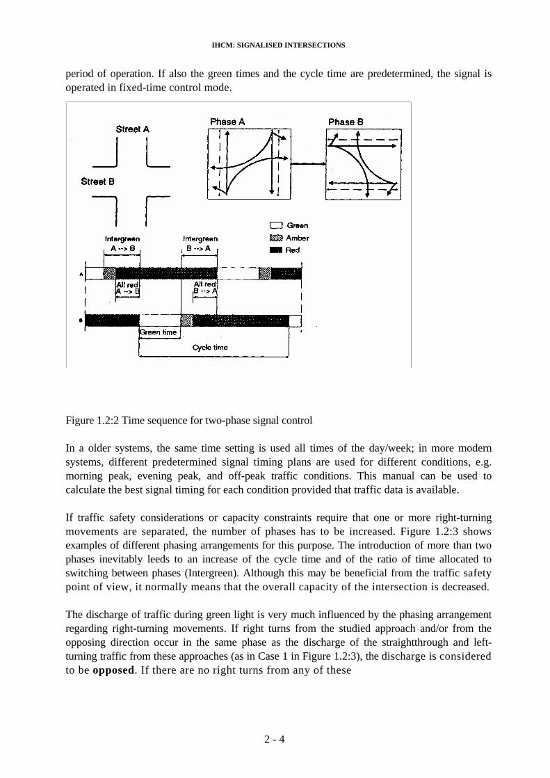
If only the primary conflicts are separated, it is possible to control the signal in two phases, one foreach of the crossing streets, as shown in Figure 1.2:2. This method can always be applied if theright-turning movements have been forbidden in the intersection. Since twophase control yields highest capacity in most cases, it is the base case in most signal analyses.
Figure 1.2:2 also illustrates the sequence of signal changes for two-phase signal control,including definitions of cycle time, green time and intergreen periods (see also Section 1.3). Thepurpose of the intergreen period (IG = amber + allred) between two consecutive signal phases is to:
.1 warn discharging traffic that the phase is terminated.
.2 certify.that the last vehicle in the green phase which is being terminated receives adequate time to evacuate the conflict zone before the first advancing vehicle in the next phase enters the same area.
The first function is fulfilled by the amber period, the second by the allred period whichserves as a clearance time between the phases.
The allred and amber periods are normally predetermined and constant throughout the
2 - 3
IHCM: SIGNALISED INTERSECTIONS
period of operation. If also the green times and the cycle time are predetermined, the signal isoperated in fixed-time control mode.
Figure 1.2:2 Time sequence for two-phase signal control
In a older systems, the same time setting is used all times of the day/week; in more modernsystems, different predetermined signal timing plans are used for different conditions, e.g.morning peak, evening peak, and off-peak traffic conditions. This manual can be used to calculate the best signal timing for each condition provided that traffic data is available.
If traffic safety considerations or capacity constraints require that one or more right-turning movements are separated, the number of phases has to be increased. Figure 1.2:3 showsexamples of different phasing arrangements for this purpose. The introduction of more than twophases inevitably leeds to an increase of the cycle time and of the ratio of time allocated to switching between phases (Intergreen). Although this may be beneficial from the traffic safetypoint of view, it normally means that the overall capacity of the intersection is decreased.
The discharge of traffic during green light is very much influenced by the phasing arrangementregarding right-turning movements. If right turns from the studied approach and/or from theopposing direction occur in the same phase as the discharge of the straightthrough and left-turning traffic from these approaches (as in Case 1 in Figure 1.2:3), the discharge is consideredto be opposed. If there are no right turns from any of these
2 - 4

IHCM: SIGNALISED INTERSECTIONS
approaches, or if the right turns are discharged when the straight-through traffic from theopposing direction has red light (as in Case 5 and 6 in Figure 1.2:3), the discharge isconsidered to be protected. In Case 2 and 3 the discharge from the north approach is partly opposed, partly protected. In Case 4 the discharge from the north and south approaches are protected, from the east and west approaches opposed.
Case Characteristics
1. Two-phase control,only primary conflicts are separated
2. Three-phase controlwith late cut-off in the north approach to increase the capacity for right turns from this direction
3. Three-phase controlwith early start of the north approach to increase the capacity for right turns from this direction
4. Three-phase controlwith separated right turns in one of the streets
5. Four-phase control with separate rightturns in both streets
6. Four-phase control with discharge of one approach at a time
Figure 1.2:3 Signal phasing arrangements for separation of right-turning movements.
2 - 5

IHCM: SIGNALISED INTERSECTIONS
1.3 DEFINITIONS AND TERMINOLOGY
Notations, terminology and definitions specific to signalised intersections are listed below (see alsogeneral definitions in Chapter 1, Section 4).
TRAFFIC CONDITIONS AND CHARACTERISTICS
pcu PASSENGER CAR UNIT Conversion factor for different vehicle typeswith regard to their green time requirement for discharge from a queue in the approach ascompared to a passenger car (i.e for passenger car/light vehicle pcu = 1.0).
Type O OPPOSED DISCHARGE Discharge with conflict between right-turningmovements and straight-through/left-turningmovements from different approaches with green in the same phase.
Type P PROTECTED DISCHARGE Discharge without any conflict between right turning movements and straight-through traffic.
LT LEFT-TURNING Index for left-turning traffic.
LTOR LEFT TURN ON RED Index for left-turning traffic permitted to passagainst red. signal.
ST STRAIGHT-THROUGH Index for straight-through traffic.
RT RIGHT-TURNING Index for right-turning traffic.
PRT RATIO OF RT Ratio of right-turning traffic etc.
Q TRAFFIC FLOW Number of traffic elements passing an undis turbed point upstream in the approach per unitof time (i.e. = traffic demand veh/h; pcu / h).
QO OPPOSING FLOW Flow of traffic in an opposing approach being discharged in the same green phase.
QRTO RIGHT-TURNING,OPPOSING TRAFFICFLOW
Flow of right-turning traffic from the opposingapproach (veh/h; pcu/h).
S SATURATION FLOW Rate of queue discharge in an approachduring given conditions (pcu per hour of green = pcu / hg).
2 - 6

IHCM: SIGNALISED INTERSECTIONS
So BASE SATURATIONFLOW
Rate of queue discharge in an approachduring ideal conditions (pcu per hour ofgreen = pcu / hg).
DS DEGREE OFSATURATION
Ratio of flow to capacity for an approach (Qxc/Sxg).
FR FLOW RATIO Ratio of flow to saturation flow (Q/S) for anapproach.
IFR INTERSECTION FLOWRATIO
Sum of the critical (= highest) flow ratios forall consecutive signal phases in a cycle (IFR =E(Q/S)cRfr).
PR PHASE RATIO Critical flow ratio divided by intersection flowratio (e.g for phase is PR = FR;/IFR)
C CAPACITY Maximum sustainable traffic flow (e.g. forapproach j: Ci = S,xgi/c; veh/h, pcu/h).
F CORRECTION FACTOR Correction factor for adjustment from ideal toactual value of a variable.
D DELAY Extra travel time required to pass an inter section as compared to a situation with nointersection.
QL QUEUE LENGTH Length of a queue of vehicles in an approach (m).
NQ QUEUE Number of queuing vehicles in an approach(veh; pcu).
Psv PROPORTION OFSTOPPED VEHICLES
Ratio of flow forced to come to a completestandstill before crossing the stopline due to the signal control.
GEOMETRIC CONDITIONS AND CHARACTERISTICS
APPROACH Area of an intersection arm for vehicles queuing before discharge across the stop-line. (If left-turning or right-turning traffic movements are separated by traffic islands, an intersection arm can consist of two or moreappro aches).
APPROACH WIDTH Width of the paved part of,the approach measured at the upstream bottleneck (m).
2 - 7

IHCM: SIGNALISED INTERSECTIONS
WENTRY ENTRY WIDTH Width of the paved part of the approach measured at the stop-line (m).
WEXIT EXIT WIDTH Width of the paved part of the approach used by the discharged traffic after crossing of theintersection (m).
We EFFECTIVE WIDTH Width of the paved part of the approach used in the capacity calculations (i.e. withconsiderations to WA, WENTRY and WEXIT andturning traffic movements; m).
L DISTANCE Length of a road segment (m).
GRAD GRADIENT Gradient of road segment in the direction of travel (+/- `yo).
ENVIRONMENTAL CONDITIONS
COM COMMERCIAL Commercial landuse (e.g. shops, restaurants,offices) with direct roadside access for pedes trians and vehicles.
RES RESIDENTIAL Residential linduse with direct roadside access for pedestrians and vehicles.
RA RESTRICTED ACCESS No or limited direct roadside accessl(e.g dueto the existence of physical barriers, frontage streets etc).
CS CITY SIZE Number of inhabitants in an urban area.
SF SIDE FRICTION Interaction between traffic flow and roadsideactivities causing a reduction of saturation flow in an approach.
SIGNAL CONTROL PARAMETERS
i PHASE Part of a signal cycle with green lightallocated to a specific combination of trafficmovements (i = index for phase no).
c CYCLE TIME Duration of a complete sequence of signal indications (e.g. between two consecutive starts of green in the same approach; sec).
2 - 8

IHCM: SIGNALISED INTERSECTIONS
g GREEN TIME Duration of the green phase in an approach (sec).
gmax MAXIMUM GREEN TIME Maximum green time permitted in a phase during vehicle actuated traffic control (sec).
g MINIMUM GREEN TIME Minimum required green time (e.g. due topedestrian crossing, sec).
GR GREEN RATIO Ratio between green time and cycle timefor an approach (CR = g/c).
IG INTERGREEN Amber + allred period between two consecutive signal phases (sec).
CT CLEARANCE TIME Time required between two consecutive signalphases for safety reasons (sec).
LT LOST TIME Difference between the cycle time and the sum of the green time in all consecutive phases (=sum of all intergreen periods during a complete signal cycle; sec).
ALLRED ALLRED TIME Time during which red signal is displayed si-multaneodsly in approaches served by two consecutive signal phases (sec).
AMBER AMBER TIME Time during which amber light after green is displayed in an approach (sec).
2 - 9

IHCM: SIGNALISED INTERSECTIONS
2. METHODOLOGY
2.1 GENERALPRINCIPLES
The methodology for analysis of signalised intersections described below is based on thefollowing main principles.
a) Geometry
The calculations are done separately for each approach. Oneintersection arm can consist of more than one approach, i.e. bedivided in two or more sub-approaches. This is the case if theright-turning and/or leftturning movements receive green signal in different phase(s) than the straight-through traffic, or if they arephysically divided by trafficislands in the approach.
For each approach or sub-approach the effective width (We) is determined with consideration tothe layout of the entry and the exit and the distribution of turning movements.
b) Traffic flow
The calculations are performed on an hourly basis for one or more periods, e.g. basedon peak-hour design flows for morning, noon and afternoon traffic conditions.
The traffic flows (Q) for each movement (left-turning QLT, straight-through QST, and right-turning QRT) are converted from vehicles per hour to passenger car units per hour using thefollowing pcu values for protected and for opposed approach types:
pcu value for approach type Vehicle type
Protected Opposed
Light veh. (LV) 1.0 1.0
Heavy veh. (HV) 1.3 1.3Motorcycle (MC) 0.2 0.4Un-motorised (UM) 0.5 1.0
Example: Q = QLV + QHV x pcuHV + QMC + QUM x pcuUM
2 - 10

IHCM: SIGNALISED INTERSECTIONS
c) Basic model
The capacity (C) of an approach to a signalised intersection can be expressed as follows:
C = S x g/c (1)
whereC = Capacity (pcu/h).S = Saturation flow, i.e. mean discharge rate from a queue in the approach during green
signal (pcu/hg = pcu per hour of green).g = Displayed green time (sec). c = Cycle time, i.e. duration of a complete sequence of signal changes (i.e. between
two consecutive starts of green in the same phase).
It is thus necessary to know or to determine the signal timing of the intersection in order tocalculate capacity and different measures of performance.
In Formula (1) above the saturation flow (S) is assumed to be constant during the duration ofgreen. In reality, however, the discharge rate starts from 0 at the beginning of green and reaches itspeak value after 10-15 seconds. It then drops slightly until the end of green, see Figure 2.1:1 below. The discharge also continues during amber and allred until it drops to 0, normally 5-10 seconds after the beginning of red signal.
Figure 2.1:1 Observed saturation flows per six second time slices
2 - 11

IHCM: SIGNALISED INTERSECTIONS
The start-up discharge causes what can be described as a Start loss of effective green time,the discharge after end of green results in an End gain of effective green time, see Figure 2.1:2.The resulting total effective green time, i.e. the green time during which the dischargeoccurs with a constant rate S, can then be calculated as
Eff. green = Displayed green time - Start loss + End gain (3)
Figure 2.1:2 Basic model for saturation flow (Akcelik 1989).
By analysis of field data from all the surveyed intersections it was concluded that the averagestart loss and end gain both were in the order of 4.8 sec. According to Formula (3) abovee theeffective green time then becomes equal to the displayed green time for the studied standardcase. The conclusion from this analysis was that the displayed green time and the peaksaturation flow rate observed in the field for each site could be used in Formula (1) above to calculate the capacity of the approach without adjustment for start loss and end gain periods.
2 - 12

IHCM: SIGNALISED INTERSECTIONS
The saturation flow (S) can be expressed as a product between a base saturation flow (So)for a set of standard conditions, and correction factors (F) for deviation of the actual conditions from a set of pre-determined (ideal) conditions.
S= S0 x Ft x F2 x F3 x F4 x Fn (2)
For protected approaches the base saturation flow So is determined as a function of theeffective approach width (We):
So = 600 x We
Corrections are then made for the following conditions:- City size CS, million inhabitants)- Side friction SF, high or low (also a function of road envi
ronment)- Gradient G, % up (+) or down (-)- Parking P, distance stopline - first parked vehicle- Turning movements RT, `y, right-turning
“ “ LT, % left-turning
For opposed approaches, the queue discharge is heavily influenced by the fact that Indonesian drivers do not respect the right-of-way rule from the left, i.e. right turningvehicles push their way through the opposing straight-through traffic. Western modelsfor this discharge, which are based on gap-acceptance theory, cannot be applied. An explanatory model based on observed driver behaviour was developed and implementedin the , manual. Generally it results in lower capacities where there is a high ratio ofright turning movements, than appropriate for corresponding Western models. Differentpcu-values for opposed approaches are also used used as described above.
The base saturation flow S. is determined as a function of effective approach width (We)and the flow of right-turning traffic in the own approach as well as in the opposingapproach, since the influence of these factors is non-linear. Corrections are then made for actual conditions regarding City size, Side friction, Gradient and Parking as in Formula 2 above.
d) Signal timing
The signal timing for fixed-time control conditions is determined based on the Webster(1966) method for minimisation of overall vehicle delay in the intersection. First the cycle time (c) is determined, and after that the length of green (gi) in each phase (i).
CYCLE TIME c = (1.5 x LT + 5)/(1 - FRcrit) (3)]
2 - 13

IHCM: SIGNALISED INTERSECTIONS
wherec = Signal cycle time (sec) LT = Total lost time per cycle (sec) FR = Flow divided by saturation flow (Q/S) FRcrit = The highest value of FR in all approaches being discharged in a signal phase.
(FRcrit) = Intersection flow ratio = sum of FRcrit for all phases in the cycle.
If the cycle time is shorter than this value there is a serious risk for over-saturation of theintersection. Too long cycle times result in increased average delay to the traffic. If F(FRcrit) isclose to or over I the intersection is oversaturated and the formula will result in very high ornegativee cycle time values.
GREEN TIME gi = (c - LT) x FRcrit/E(FRcrit) (4)
where gi = Displayed green time in phase i (sec)
The performance of a signalised intersection is generally much more sensitive to errors in thegreen time distribution than to a too long cycle time. Even small deviation from the green ratio (g/c) determined from Formula 3 and 4 above results in high increase of the averagedelay in the intersection.
e) Capacity and degree of saturation
The approach capacity (C) is obtained by multiplication of the saturation flow with the greenratio (g/c) for each approach, see Formula (l) above.
The degree of saturation (DS) is obtained as
DS = Q/C = Q x c/(S x g) (5)
f) Level of performance
Different measures of level of performance can be determined based on the traffic flow (Q), degree of saturation (DS) and signal timing (c and g) as described below:
QUEUE LENGTH
The average number of queuing pcu at the beginning of green NQ is calculated as the numberof pcu that remain from the previous green phase NQ1 plus the number of pcu that arriveduring the red phase (NQ2:
NQ = NQ1 + NQ2 = (DS-U.5) / (1-DS) + Q x (c-g) (6)
2 - 14

IHCM: SIGNALISED INTERSECTIONS
For design purposes the manual includes provision for adjustment of this average value to adesired level of probability for overloading.
The resulting queue length QL is obtained by multiplication of NQ with the average areaoccupied per pcu (20 sqm) and division with the entry width.
QL = NQ x 20/ WENTRY (m) (7)
PROPORTION OF STOPPED VEHICLES
The proportion of stopped vehicles pSV,i.e. the ratio of vehicles that have to stop because of the redsignal before passing the intersection, i calculated as
pSV = 1 + NQ/c - g/c (8)
where c is the cycle time and g the green time in the studied approach.
DELAY
The average delay for an approach can be determined from the following formula (based onWebster 1966):
Di = (cx(1-GR)2/(2x(1-GRxDS) + DS2/(2x(1-DS)xQi)l x 0.9
where
D = Mean delay for approach (sec/pcu)GR = Green ratio (g/c)DS = Degree of saturationc = Cycle time (sec)Q = Traffic flow (pcu /sec)
Observe that the calculation result are not valid if the capacity of the intersection is influenced by "external" factors such as blocking of an exit due to downstreamcongestion, manual police control etc.
2 - 15

IHCM: SIGNALISED INTERSECTIONS
Protected discharge from a signalised approach, i.e. no conflict between right-turningvehicles and traffic from the opposing direction.
In protected approaches without median, right-turning vehicles frequently use the opposingdriveway when they make their turn.
2 - 16

IHCM: SIGNALISED INTERSECTIONS
In opposed approaches right-turning vehicles usually do not respect the right-of-way of straight-through traffic
If there is no median, right-turning vehicles block the path of the straight through movement by “cutting” into the opposing driveway.
2 - 17

IHCM: SIGNALISED INTERSECTIONS
2.2 OVERVIEW OF THE CALCULATION PROCEDURE
A flow chart of the calculation procedure is illustrated below. The different we dscribed in detailin Section 3.
Figure 2.2:1 Flow chart for analysis of signalized interactions
2 - 18
IHCM: SIGNALISED INTERSECTIONS
The following forms are used for the calculations:
SIG-I GEOMETRY, TRAFFIC CONTROL, ENVIRONMENT
SIG-II TRAFFIC FLOW
SIG-111 CLEARANCE TIME, LOST TIME
SIG-IV SIGNAL TIMING, CAPACITY
SIG-V DELAY, QUEUE-LENGTH, NO OF STOPPED VEHICLES
The forms are presented in Appendix 2:1 at the end of the chapter concerning signalised intersections.
2.3 GUIDELINES FOR APPLICATION
2.3.1 Types of application of the manual
The manual can fulfill many different needs and types of calculations for signalised intersections as exemplified below:
a) Planning
Given: Daily traffic flows (AADT). Task: Determination of layout and type of control. Example: Determination of intersection layout and phasing for a planned
intersection with given traffic demand.Comparisons with other modes of control and types of traffic fa-cilities such as unsignalised control, roundabout layout etc.
b) Design
Given: Layout and traffic flow (daily or hourly). Task: Determination of recommended design. Example: Signalisation of a previously unsignalised intersection.
Betterment of an existing signalised intersection, e.g. with new signal phasing and approach design. Design of a new signalised intersection.
c) Operation
Given: Geometric design, signal phasing and hourly traffic flows.Task: Calculation of signal timing and capacity.Example: Updating of the signal timing for different periods of the day.
Estimation of reserve capacity and expected need for capacity im provement and/or changed signal phasing as a result of annualtraffic growth.
2 - 19
IHCM: SIGNALISED INTERSECTIONS
The signal timing calculated in the manual is recommended for fixed-time control for thetraffic conditions used as input data. In order to be on the safe side against traffic fluctuations, a10% proportional increase of the green times and a corresponding increase of the cycle time isrecommended for installation purpose. If the timing is used for traffic actuated control, the maximum green times should be set 25-40% larger than the green times at fixed-time control.
The signal timing method can also be used to determine the minimum cycle time in a systemwith fixed-time coordination of traffic signals (i.e. the whole system will operate with thehighest cycle time required for any of its intersections).
The methodology used at each level is essentially the same, with execution of calculations of signaltiming, capacity and level of performance for successive sets of input data until a satisfactorysolution to the given problem has been obtained.
2.3.2 Default values
On the operational level (c above) all required data inputs are normally obtainable since the calculations refer to an already existing, signalised intersection. For planning and design usehowever a number of assumptions have to be made to be able to apply the calculationprocedures described in Section 3. Preliminary guidance regarding assumptions and defaultvalues for use in these cases are presented below.
a) Traffic flows
If only daily traffic flows (AADT) are available without any knowledge of the hourly traffic distribution, the design hourly flows can be estimated as a percentage of the AADT asfollows:
Type of city and road Percentage factor K KxAADT = Design flow/h
Cities > I M inhabitants - Roads in commercial areas and arterial roads
7-8%
- Roads in residential areas 8-9%
Cities < I M inhabitants - Roads in commercial areas and arterial roads
8-10%
- Roads in residential areas 9-12%
If the distribution of turning movements is unknown and cannot be estimated, the followingprovisional default values can be used (unless some of the turning movements will beforbidden):
2 - 20

IHCM: SIGNALISED INTERSECTIONS
Right-turning 15% of total approach flow Left-turning 15% of total approach flow
The following default values for traffic composition can be used in lack of better estimates :
Traffic composition % City size M inhabitants Light veh.
LVHeavy veh.
HVMotorcycles
MCUnmotorised
UM> 3 M 1 – 3 M 0.3 – 1 M < 0.3 M
5952.53460
4.53.53.02.5
35.5394933
1.05.0144.5
b) Signal phasing and timing
If the number and types of signal phases are not known, two-phase control should be used as abase case. Separate control of right-turning movements should normally only be considered if a turning movement exceeds 200 pcu/h.
Signal timing default values recommended for use, in Step C below are
Intergreen time (amber + allred) - Small intersection 5 sec per phase- Large intersection > 6 sec per phase
c) Approach widths
The following approach widths can be used as start-up assumptions for the analysis of asignalised intersection on the design and planning level if other information is lacking:
Total incoming traffic flowin the intersection (pcu/h)
Average approach width(m)
< 2500 4.52500 -4000 74000 -5000 10 (sep. RT lanes) > 5000 Larger design
The approach widths naturally have to be adjusted to imbalances in the ratio of flow betweenthe intersecting roads and their approaches.
2 - 21

IHCM: SIGNALISED INTERSECTIONS
The very high ratio motorcycle in Indonesian cities result in big groups of motorcyclesassembling at the stop-line before the start of green.
2 - 22

IHCM: SIGNALISED INTERSECTIONS
3. CALCULATION PROCEDURE
The procedures required for calculation of signal timing, capacity and level of performanceare described below step-by-step _in the following order (see also the flow chart in Figure 2.2:1 above):
STEP A: INPUT DATA A-1: Geometric, traffic control and environmental conditions
A-2: Traffic flow conditions
STEP B: SIGNALISATION B-1: Signal phasing
B-2: Clearance time and lost time
STEP C: SIGNAL TIMING C-1: Approach type
C-2: Effective approach widthC-3: Base saturation flow
C-4: Correction factors C-5: Flow/saturation flow ratio
C-6: Cycle time and green times
STEP D: CAPACITY D-1: Capacity
D-2: Need for revisions
STEPE: LEVEL OF PERFORMANCE E-1: Preparations E-2: Queue length
E-3: Stopped vehicles E-4: Delay
Blank forms for the calculations are presented in Appendix 2:1, and worked examples can befound in Section 4. Basically the same procedure is followed for all types of applications asdescribed in Section 2.3, the main difference only being in the degree of detail in the inputdata.
2 - 23

IHCM: SIGNALISED INTERSECTIONS
STEP A: INPUT DATA
Step A-1: GEOMETRIC, TRAFFIC CONTROL AND ENVIRONMENTALCONDITIONS (Form SIG-I.).
Information to be filled in the top part of Form SIC-I:
- GeneralFill in Date, Handled by,.City, Intersection, Case (e.g. Alt. 1) and Period (e.g. AM peak1993) in the head of the form.
- City sizeEnter the population of the urban area (to the nearest 0.1 M inhabitants).
- Signal phasing and timingUse the boxes under the head of Form SIG-1 to draw the existing phase diagrams (ifavailable). Enter the existing green (g) and intergreen (IC) times in each phase box, and enter the cycle time and the total lost time (LT = EIG) for the case studied (if available).
- Left turn on red LTORIndicate in the phase diagrams in which approaches) that Left turn on red is permitted (i.e. the turn can be made in all phases without consideration to thesignals).
Use the empty space in the middle part of the form to make a sketch of the intersection, andenter all required geometric input data:
- Layout and position of approaches, traffic islands, stoplines, pedestrian crossings, lanemarkings and arrows.
- Width (to the nearest tenth of a meter) of the paved part of approaches, entries and exits.
- Length of lanes with restricted length (to the nearest m).
- Draw an arrow indicating the direction of North on the sketch.
If the layout and design of the intersection is not known, see Section 2.3 above regarding startup assumptions for the analysis.
Enter data on other site conditions which are relevant for the studied case in the table at thebottom part of the form:
2 - 24

IHCM: SIGNALISED INTERSECTIONS
- Approach code (Column 1)Use North, South, East, West or any other clear indication to name the approaches. Observe that an intersection arm can be divided by traffic islands in two or moreapproaches.
- Road environment type (Column 2)Enter Road environment type (COM = Commercial; RES = Residential; RA = Restrictedaccess) for each approach (definitions see. Section 1.3).
- Level of side friction (Column 3) Enter the side friction level:
High: The discharge rate at the entry and the exit is reduced by roadside activity in the approach such as public transit stops, pedestrians walking along or crossing the approach, exits and entries to roadside properties etc.
Low: The discharge rate at the entry and exit is not reduced by side friction of thetypes described above.
- Median (Column 4)Enter if there is a median at the right side of the stopline in the approach (Yes/ No).
- Gradient (Column 5) Enter gradient in % (uphill = + % ; downhill = -%)
- Left turn on red (Column 6)Enter if Left turn on red (LTOR) is permitted (Yes/No) in the approach (additional to showing it in the phase diagrams as described above).
- Distance to parked vehicle (Column 7)Enter what the normal distance between the stop-line and the first parked vehicleupstream in the approach is for the conditions studied.
- Approach width (Column 8-10)Enter from the sketch the width (to the nearest tenth of a meter) of the paved part of each Approach (upstream of turning point for LTOR), Entry (at the stop-line) andExit (bottleneck after passing the cross road).
- CommentsRecord on a separate sheet any other information which you think might influence the capacity of the approach.
2 - 25

IHCM: SIGNALISED INTERSECTIONS
STEP A-2: TRAFFIC FLOW CONDITIONS
- If detailed traffic data with distribution on vehicle types for each turning movement isavailable, Form SIG-I1 is recommended for use. Enter the traffic flow data for each vehicle type in veh/h In Column 3, 6, 9 and 12. In other cases it might be preferable touse a simpler form of data presentation, and to enter the results directly into Form SIG-IV.(Default traffic input values: See Section 2.3.2 above).
Several sets of traffic flow data may be needed for analysis of different periods, e.g morning peak hour, noon peak hour, afternoon peak hour, off-peak hour etc.
Observe: If Left turn on red (LTOR) is permitted and does not interfere with theother traffic in the approach (i.e. LTOR vehicles can pass the queue of straightthroughand right-turning vehicles formed in the approach during red light) the LTORmovement should be excluded in Form SIG-II.
- Calculate the traffic flow in pcu/h for each vehicle type for protected and/oropposed discharge conditions (whichever is relevant depending upon the signal phasing and permitted right-turning movements) using the following pcu values:
pcu - valuesVehicle type Protected
approachOpposedapproach
LV 1.0 1.0
HV 1.3 1.3
MC 0.2 0.4
UM 0.5 1.0
Enter the results in Columns 4-5, 7-8, 10-11, 13-14.
- Calculate the total traffic flow in veh/h and pcu/h in each approach for protectedand/or opposed discharge conditions (whichever is relevant depending upon the signal phasing and permitted right-turning movements). Enter the results in Columns15-17.
- Calculate for each approach the ratio of left-turning pl,i•, and the ratio of rightturningpRT, and enter the results in Columns 18 and 19 in the respective rows for LT andRT flows:
2 - 26

IHCM: SIGNALISED INTERSECTIONS
STEP B: SIGNALISATION
Step B-1: SIGNAL PHASING (Form SIG-IV)
If the calculations shall be performed for other than the existing signal phasing scheme as drawn in Form SIG-I, a signal phasing scheme must be chosen as a start-up alternative for evaluation. Different types of signal phasing have been shown in Section 1, Figure 1.2:3.
PROCEDURE
- Select signal phasing.As a preliminary advice (awaiting the traffic engineering guidelines to be developedin Phase 3 of the HCM project) two-phase control should be tried as a base case, since itusually yields higher capacity and lower average delay than other types of signalphasing. Separate control of a right-turning movement is normally only preferablefrom a capacity point of view if it exceeds 200 pcu/h. It may however be requiredfor traffic safety reasons in special cases.
- Sketch the chosen signal phasing in the boxes reserved for this purpose in Form SIG-IV.
2 - 27

IHCM: SIGNALISED INTERSECTIONS
Step B-2: CLEARANCE TIME AND LOST TIME (Form SIG-III).
- Determine the required clearance times and the total lost time in the intersection asdescribed below.
- Enter the resulting total lost time LT at the bottom of Column 4.in Form SIC-IV.
For operational and design analysis a detailed calculation of the clearance times and the total losttime with the help of Form SIC-III as described below is recommended. In analysis performedfor planning purposes, the following intergreen times (amber + allred) can be assumed asdefault values:
Intersection size Mean approach width
Intergreen timedefault values
Small 3 - 6 m 5 sec/phase Medium 6 - 9 m 6 sec/phaseLarge > 9 m 7 sec/phase
PROCEDURE FOR DETAILED CALCULATIONS
The required clearance time (CT) must allow for the last evacuating vehicle to clear the conflictpoint before arrival of the first advancing vehicle from the next phase to the same point. CTIs a function of the speed and the distances for evacuating and advancing vehicles from thestop-line to the conflict point, and of the length of the evacuating vehicle, see Figure B-2:1 below.
Figure B-2:1 Critical conflict point and distances for evacuation and advancement.
2 - 28

IHCM: SIGNALISED INTERSECTIONS
The critical conflict point in each phase (i) is the point that yields the largest resultingclearance time CT:
CTi = l ( LEV + IEV) / VEV - LAV/ V,AVlmax
Where LEV, LAV = Distance from stop-line to conflict point for evacuatingresp advancing vehicle (m)
lEV = Length of evacuating vehicle (m) VEV
, VAV = Speed of evacuating resp advancing vehicle (m/sec).
Figure B-2:l illustrates a case with critical conflict points identified for both crossing vehiclesand crossing pedestrians.
The values chosen for VEV, VAV and Irv depend upon the traffic composition and the speedconditions at the site. The following temporary values could be chosen in lack of Indonesian regulations on this matter:
Speed of advancing veh VAV 10m/sec (motor vehicles) Speed of evacuating veh. VrV. 10 m/sec (motor vehicles)
“ 3 m/sec (un-motorised)“ 1.2 m/sec (pedestrians).
Length of “ IEV: 5 m (LV or HV)“ “: 2 m (MC or UM)
The calculations are performed with the help of Form SIG-Ill.
The allred periods between the phases should be equal or greater to the clearance times.
When the allred times for each phase change have been determined, the total lost time (LT) forthe intersection can be calculated as the sum of the intergreen periods:
LT = (allred + amber); = IGj
The amber period in urban traffic signals in Indonesia is normally 3.0 sec.
2 - 29

IHCM: SIGNALISED INTERSECTIONS
STEP C: SIGNAL TIMING
Step C includes determination of the following factors:
C – 1 : Approach typeC – 2 : Effective approach widthC – 3 : Base saturation flowC – 4 : Correction factorsC – 5 : Flow/saturation flow ratioC – 6 : Cycle time and green times
The calculations are entered into Form SIG-IV SIGNAL TIMING AND CAPACITY.
Step C-1: APPROACH TYPE
- Enter identification of each approach in a separate row in Form SIG-IV Column 1.
- Enter the number of the phase during which each approach has green light in Column 2.
- Determine the type of each approach (P or 0) with the help of Figure C-1:1 below,and enter the results in Column 3.
- Make a sketch showing the resulting directional flows (Form SIG-11 Column 16-17) inpcu/h in the upper left box in Form SIG-IV (select the appropriate results for protected (Type P) or opposed conditions (Type 0) as documented in Column 3).
- Enter the ratio of turning vehicles (PLTOK or p),r, PKT) for each approach (fromForm SIG-11 Column 18-19) in Columns 4-6.
- Enter from the sketch the flow of right-turning vehicles in pcu/h in the own direction (QRT) in Column 7 for each approach (from Form SIG-11 Column 16). Enteralso for approaches of type 0 the flow of right-turning vehicles in the opposing direction (QRTO) in Column 8 (from Form SIG-II Column 17).
2 - 30

IHCM: SIGNALISED INTERSECTIONS
ApproachType
Description Examples of approachConfigurations
One-way street: One-way street: T-junction
Two-way streets, restrictedRight-turning movements
Two way street, separate signal Phase for each direction
ProtectedP
DischargeWithout conflictWith trafficFrom the opposing direction
Two-way street, discharge of the Opposing directions in the same phase. All right-turns not restricted.
OpposedO
Discharge withConflict with Traffic fromThe opposing direction
Figure C-1:1 Determination of approach type
2 - 31

IHCM: SIGNALISED INTERSECTIONS
Step C-2: EFFECTIVE APPROACH WIDTH
- Determine the effective width (W.) of each approach based on the information aboutapproach width (WA), entry width (WENTRY) and exit width (WEXIT) from theForm SIG-1 (the sketch and Column 8 - 10) as follows, and enter the result in Column 9 InForm SIG-IV:
a) For all approach types (P and O):
If Left-turn-on-red (LTOR) is permitted and does not interfere with the other traffic in the approach (i.e. LTOR vehicles can bypass the queue of straigh-through and right-turning vehicles in the approach during red signal, which can generally be assumed if WLTOK > 2 m), the effective width is determined as the smallest value of WA - WLTOR and WENTRY:
The LTOR movement should thenbe excluded from the remainingcalculations (i.e Q=QST+QRT inForm SIC IV). Proceed to b) below for a check of exit conditions (onlyfor appr. type P).
The LTOR movement is included in the remaining analysis.
Figure C-2:1 Determination of effective width
b) Control for approach type P only:
Check if the width of the approach exit is sufficient: WEXIT > WENTRY x (1 - PRT – PI.T - PLTOR)
If this condition is met, We is determined as in 1) above. If the condition is not met, W. should be set equal to WEX,T, and the remaining analysis for this approachis conducted for the straight-through portion of the traffic only (i.e. Q = QST in FormSIG-IV Column 18).
2 - 32

IHCM: SIGNALISED INTERSECTIONS
Step C-3: BASE SATURATION FLOW
- Determine the base saturation flow (S.) for each approach as described below, and enter the results in Column 10:
a) For approach type P (protected discharge):
So = 600 x We pcu/hg, see Figure C-3:1
Figure C-3:1 Base saturation flow for approach type P.
b) For approach type 0 (opposed discharge):
So is determined from Figure C-3:2 (for approaches without separate right-turninglanes), and from Figure C-3:3 (for approaches with separate right-turning lane) as a function of We QRT and QRTO.
Use the figures to obtain the saturation flow values for cases with approach width larger and smaller than the actual We and calculate the resulting value by interpolation.
2 - 33

IHCM: SIGNALISED INTERSECTIONS
Example :
Without sep. RT lane: QRT = 125 pcu/h; QRTO, = 100 pcu/hActual We = 5.4 m
Obtain from Figure C-3:2S6.0 = 3000 ; S5.0 = 2440
CalculateS5.4 = (5.4 - 5.0) x (S 6.0 – S5.0) + S5.0 = 0.4(3000 - 2440) + 2440
= 2664 – 2660
2 - 34

IHCM: SIGNALISED INTERSECTIONS
Figure C-3:2 So for approaches type O without separate right-turning lane
2 - 35

IHCM: SIGNALISED INTERSECTIONS
Figure C-3:3 So for approach type O with separate right-turning lane.
2 - 36

IHCM: SIGNALISED INTERSECTIONS
Step C-4: CORRECTION FACTORS
a) Determine the following correction actors for the base saturation flow valuefor both approach type P and O as follows:
- The City size correction factor FCS .is determined from Table C-4:3 as a function of the city size recorded in Form SIG-I. The result is entered in Column 11.
City population(M. inhabitants)
City size correction factor FCS
> 3.0 1.051.0-3.0 1.00
0.3- 1.0 0.94< 0.3 0.83
Table C-4:3 City size correction factor FCS
- The Side friction correction factor FSF is determined from Table C-4:4 as a function ofRoad environment type and Side friction recorded in Form SIG-I. The result is enteredin Column 12. If the side friction is not known, it can be assumed to be high in order not to over estimate capacity.
Correction factor FSFRoad environment
High side friction Low side frictionCommercial 0.94 1.00Residential 0.97 1.00Restricted Access 1.00 1.00
Table C-4:4 Correction factor .for Road environment type and Side friction
- The Gradient correction factor FG is determined from Figure C-4:1 as a function ofthe gradient (GRAD) recorded in Form SIG-1, and the result is entered in Column 13 inForm SIG-IV.
Figure C-4:1 Correction factor for gradient FG
2 - 37

IHCM: SIGNALISED INTERSECTIONS
- The Parking correction factor FP is determined from Figure C-4:2 as a function of the distance from the stop-line to the first parked vehicle (Column 7 in Form SIG-I) andthe approach widtih (WA,Column 9, in Form SIG-IV). The result is entered in Column 14. This factor can also be applied for cases with restricted length of leftturning lanes.
FP can also be calculated from the. following formula, which includes the effectof the length of the green time:
FP = [Lp/3 -(WA - 2) x (Lp/3 - g) /WA]/g
whereLp = Distance between stop-line and first parked vehicle (m)
(or length of short lane). WA = Width of the approach (m).g = Green time in the approach (sec).
Figure C-4:2 Correction factor for effect of parking and short left-turn lanes Fp
2 - 38

IHCM: SIGNALISED INTERSECTIONS
b) Determine the following correction factors for the base saturation flow value only forapproach type P as follows:
- The Right Turn correction factor FRT is determined as a function of ratio of right-turning vehicles PRT (from Col. 6) as follows, and the result is entered inColumn 15:
Only for Approach type P; No median; Two-way street:
Calculate FRT = 1.0 + PRT x 0.26 , or obtain the valuefrom Figure C-4:3 below
Figure C-4:3 Correction factor for right turns FRT. (only applicable for approachtype P, two-way streets)
Explanation:On two-way streets without median, the right-turning vehicles during protected discharge (approach type P) have a tendency to cross the centerline before the stopline when completing their turn. This causes a marked increase of the saturation flow athigh ratio of right-turning traffic.
2 - 39

IHCM: SIGNALISED INTERSECTIONS
- The Left turn correction factor FLT is determined as a function of the ratio of leftturns PLT as recorded in Column 5 in Form SIG-IV, and the results are entered in Column 16.
Observe : Only for Approach type P without LTOR:
Calculate FLT = 1.0 - PLT x 0.16, or obtain the value from Figure C-4:4 below
Figure C-4:4 Correction factor for effect of left turn FLT (only applicable forapproach type P with no left turn on red)
Explanation:In protected approaches without provisions for left turn on red, the left-turningvehicles tend to slow down and decrease the saturation flow of the approach. Due. to the generally slower discharge of traffic in opposed approaches (type O), no correction for the influence of the ratio of left turns is needed.
c) Calculate the adjusted value of saturation flow S
The adjusted saturation flow value is calculated as
S = So x FCS x FSP x FG.x FP x FRT x FLT x pcu/hg
Enter the value in Column 17.
2 - 40

IHCM: SIGNALISED INTERSECTIONS
Step C-5: FLOW/SATURATION FLOW RATIO
- Enter the relevant traffic flow for each approach (Q) from Form SIG-I1 Column 16 (Protected) or Column 17 (Opposed) into Column 18 in Form SIG-IV.
Observe:
- If LTOR shall be excluded from the analysis (see Step C-2, item 1-a) only thestraight-through and the right-turning movements should be included in the Q-value to be entered in Column 18.
- If We = WE T (see Step C-2, item 2) only the straight-through movement should beincluded in the Q-value in Column 18.
- Calculate the Flow Ratio (FR) for each approach and enter the results in Column 19:
FR = Q/S
- Identify the critical (= highest) flow ratio (FRCRIT) in each phase by encircling it inColumn 19.
- Calculate the Intersection flow ratio (IFR) as the sum of the encircled (= critical) valuesof FR in Column 19, and enter the result in the box at the bottom of the Column 19.
IFR = (FRcrit)
- Calculate the Phase Ratio (PR) for each phase as the ratio between FRCRIT and IFR, andenter the results in Column 20.
PR = FRcrit/IFR
2 - 41
IHCM: SIGNALISED INTERSECTIONS
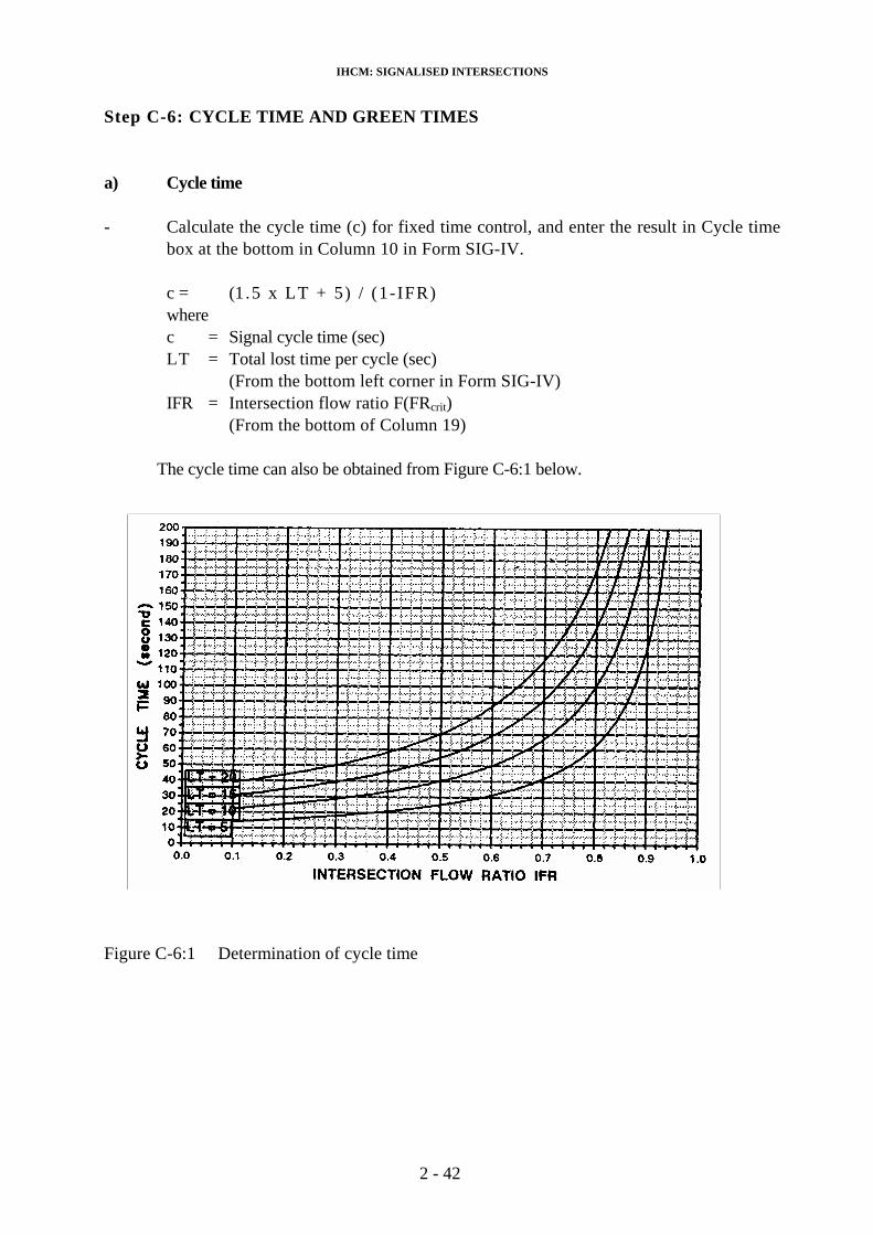
Step C-6: CYCLE TIME AND GREEN TIMES
a) Cycle time
- Calculate the cycle time (c) for fixed time control, and enter the result in Cycle timebox at the bottom in Column 10 in Form SIG-IV.
c = (1.5 x LT + 5) / (1-IFR)wherec = Signal cycle time (sec) LT = Total lost time per cycle (sec)
(From the bottom left corner in Form SIG-IV)IFR = Intersection flow ratio F(FRcrit)
(From the bottom of Column 19)
The cycle time can also be obtained from Figure C-6:1 below.
Figure C-6:1 Determination of cycle time
2 - 42

IHCM: SIGNALISED INTERSECTIONS
If alternative signal phasing schemes are evaluated, the one which yields the lowestvalue of (IFR + LT/c) is the most efficient.
- Adjust the calculated cycle time with the regard to the recommended limits below(based on traffic engineering judgement), and enter the adjusted value below the calculated cycle time at the bottom in Column 10 in Form SIG IV:
Type of control Feasible cycle time(sec)
Two-phase control 40- 80Three-phase control 50 - 100
Four phase control 80- 130
The lower values refer to intersections with street widths < 10 m, the higher values to wider streets. Cycle times lower than the recommended values will lead to dif-ficulties for pedestrians to cross the streets. Cycle times in excess of 130 secondsshould be avoided other than in very special cases (very large intersections), since itoften results in loss cof overall capacity.
If the calculations yield a much higher cycle time than the recommended limits, it indicates that the capacity of the current layout of the intersection is insufficient. Thisproblem is dealt with in Step E below.
b) Green time
Calculate green times (g) for each phase:
gi = (c - LT) x PRi
wheregi = Displayed green time in phase i (sec)c = Adjusted cycle time (sec)
(From bottom of Column 10)LT = Total lost time per cycle
(From bottom of Column 4)PRi = Phase ratio FRcrit/ (FRcrit)
(From Column 20)
Shorter green times than 10 seconds should be avoided, since they may result in excessive driving against red light and difficulties for pedestrians to cross the road. If the green timesneed to be adjusted, the corresponding adjustment must also be made of the cycle time. Enterthe adjusted green times in Column 21.
2 - 43

IHCM: SIGNALISED INTERSECTIONS
STEP D: CAPACITY
Step D includes determination of the capacity of each approach, and a discussion of revisions tobe made if the capacity is insufficient.
The calculations are entered into Form SIG-IV.
Step D-1: CAPACITY
- Calculate the capacity C of each approach and enter the result in Column 22:
C = S x g/c where the values for S are obtained from Column 17, g and c from Column 10 (bottom).
- Calculate the Degree of saturation DS for each approach , and enter the result in Column23:
DS = Q/C where the values for Q and C are obtained from Column 18 and 22.
If the signal timing has been correctly done, DS will be the same in all criticalapproaches.
2 - 44

IHCM: SIGNALISED INTERSECTIONS
Step D-2: NEED FOR REVISIONS
If the degree of saturation (DS) is close to or higher than 1.0, the intersection is oversaturated,which will lead to accumulating queues during peak-traffic conditions. The possibility to increasethe capacity of the intersection by any of the following measures should therefore beconsidered:
a) Increase of approach width
If it is possible to increase the approach widths, the best effect of such a measure will beobtained if the width is increased in the approaches with the highest critical FR value(Column 19).
b) Changed signal phasing
If approaches with opposed discharge (type 0) and high ratio of right-turning traffic(PRT) show high critical FR values, an alternative phasing scheme with separatephase for right-turning traffic might be appropriate. See Section 1.2 above for selectionof signal phasing. Introduction of separate phases for right-turning traffic may have to accompanied with widening measures as well.
If the intersection is operated in four phases with separate discharge of each approach, as phase scheme with only two phases might give higher capacity, provided that the right-turning movements are not too high (< 200 pcu/h).
c) Prohibition of right-turning movement(s)
The prohibition of one or more right-turning movements will normally increasecapacity, particularly if it leads to a reduction of the number of phases required. Proper traffic management planning is however required to make sure that the trips served by the right-turning movements to be forbidden can be accomplished withoutexcessive detours and disturbances to adjacent intersections.
2 - 45

IHCM: SIGNALISED INTERSECTIONS
STEP E: LEVEL OF PERFORMANCE
Step E includes determination of the level of performance of the signalised intersection in terms of queue-length, no. of stopped vehicles and delay. The calculations are performedusing Form SIG-V.
Step E-1: PREPARATIONS
- Fill in the information required in the head of Form SIG-V.
- Enter approach code in Column I (same as Column 1 in Form SIC-IV).
- Calculate the traffic flow for each approach in pcu/sec by dividing the value of Q (Form SIC-IV Column 18) with 3600, and enter the result in Column 2.
- Enter the flow ratio in Column 3 (from Column 19 in Form SIG-1V).
- Calculate the green ratio CR = g/c from the adjusted results in Form SIC-IV(Columns 10 bottom and Column 21), and enter the result in Column 4.
- Enter the degree of saturation in Column 5 (from Eorm SIG-IV Column 23).
2 - 46

IHCM: SIGNALISED INTERSECTIONS
Step E-2: QUEUE LENGTH
- Use the calculate value of degree of saturation DA (Column 5) to calculate thenumber of queuing pcu (NQ1) that remain from the previous green phase. Use the formula or Figure E-2:1 below, and enter the result in Column 6.
5.015.0DSFor DS > 0.5 NQ1 = ; for DS < 0.5 NQ1 = 0
Figure E-2:1 Number of queuing vehicles that remain from the previous greenphase NQ1
- Calculate the number of queuing pcu that arrive during the red phase (NQ2), and enter the result in Column 7.
NQ2 = Q x (c - g)
- Obtain the total number of queuing vehicles and enter the result in Column 8:
NQ = NQ, + NQ2
2 - 47

IHCM: SIGNALISED INTERSECTIONS
- Use Figure E-2:2 below to adjust NQ with regard to the desired probability foroverloading POL(%), and enter the resulting value NQMAX in Column 9. Forplanning and design POL < 5% is recommended, for operation a POL = 5 - 10% might beacceptable.
- Calculate the queue length QL by multiplying NQMAX with the average area occupied per pcu (20 sqm) and dividing with the entry width, and enter the result inColumn 10.
QL = NQMAX x 2O / WENTRY (m)
Figure E-2:2 Calculation of no. of queing pcu NCMAX
2 - 48

IHCM: SIGNALISED INTERSECTIONS
Step E-3: STOPPED VEHICLES
- Calculate the proportion of stopped vehicles pSV from the formula below or usingFigure E-3:1. pSV is a function of NQ (Column 8) divided by the cycle time, and thegreen ratio (Column 4). Enter the result in Column 11.
NQ gc c
PSV = 1 + -
If a higher value than 1.0 is obtained, select 1.0 (= all vehicles are stopped at least once).
Figure E-3:1 Proportion of stopped vehicles pSV
- Calculate the number of stopped vehicles Nsv and enter the results in Column 12:
NSV = Q x pSV
- Calculate the average proportion of stopped vehicles for the whole intersection andenter the result at the bottom of Column 12:
PSV,TOT = NSV/ Q
2 - 49

IHCM: SIGNALISED INTERSECTIONS
Step E-4: DELAY
The delay for an approach can be determined from the following formula (based on Webster1966):
Dj =(A, x c + Bj / Qj) x 0.9
where
Di = Mean delay for approach j (sec/pcu)A1 = (1 - GR)2 / 2 x (1 - CRxDS)Bi = DS2 / 2(1 - DS)c = Cycle time (sec)Qj =. Traffic flow for approach j (pcu/sec)
Determine the value of A, from the formula above or from Figure E-4:1 below by enteringwith the value of degree of saturation (from Column 5) on the horisontal axis, the greenratio (from Column 4), and reading the resulting A value on the vertical axis. Enter thevalue of A in Column 13.
Figure E-4:1 Determination of Aj in the delay formula
2 - 50

IHCM: SIGNALISED INTERSECTIONS
- Multiply the value of Ai (Column 13) with the cycle time and enter the value in Column 14.
- Determine the value of B, from the formula or from Table E-4:1 below by entering with the value of degree of saturation (from Column 5). Enter the value in Column 15.
Bi
Degree of saturaton
DS
0.00 0.01 0.02 0.03 0.04 0.05 0.06 0.07 0.08 0.09
0.1 0.006 0.007 0.008 0.010 0.011 0.013 0.015 0.017 0.020 0.022
0.2 0.025 0.028 0.031 0.034 0.038 0.042 0.046 0.050 0.054 0.059
0.3 0.064 0.070 0.075 0.081 0.088 0.094 0.101 0.109 0.116 0.125
0.4 0.133 0.142 0.152 0.162 0.173 0.184 0.196 0.208 0.222 0.235
0.5 0.250 0.265 0.282 0.299 0.317 0.336 0.356 0.378 0.400 0.425
0.6 0.450 0.477 0.506 0.536 0.569 0.604 0.641 0.680 0.723 0.768
0.7 0.817 0.889 0.928 0.987 1.05 1.13 1.20 1.29 1.38 1.49
0.8 1.60 1.73 1.87 2.03 2.21 2.41 2.64 2.91 3.23 3.60
0.9 4.05 4.60 5.28 6.18 7.38 9.03 11.5 15.7 24.0 49.0
Table E-4:1 Determination of Bi
- Divide the value of Bi (Column 15) with Q (column 2) and enter the value inColumn 16.
- Calculate the average delay D (sec/pcu) as the sum of Column 14 and 16 multipliedby 0.9 (see the formula above) and enter the resulting delay values in Column 17.
- Calculate the total delay in seconds by multiplying the average delay (Column 17) with the traffic flow (Column 2), and enter the results in Column 18.
- Calculate the average delay for the whole intersection D, by dividing the sum of thedelay values in Column 18 with the sum of the traffic flow values in Column 2:
D1 = (Q x Di)/ Qi
Enter the value in the bottom box in Column 18.
- The average delay can be used as an indicator of the level of service of each individualapproach as well as of the intersection as a whole.
2 - 51

IHCM: SIGNALISED INTERSECTIONS
In the U.S. Highway Capacity Manual (TRB Special Report 209 1985) the following relation between level of service and delay is given:
Level of Service Stopped delay (sec/ veh)
A <5B 5.1 - 15
C 15.1 - 25
D 25.1 - 40
E 40.1 - 60
F > 60
(Corresponding service levels for use in Indonesia will developed in the third phase of the HCM project)
2 - 52

IHCM: SIGNALISED INTERSECTIONS
4. WORKED EXAMPLES
EXAMPLE 1
Intersection: JI Iskandarsyah - JI Wijaya, Jakarta
Task: a) Update the signal timing for the AM peak hour and calculate capac-ity and level of performance with the new signal timing.
b) Calculate signal timing and degree of saturation if the west approachon Jl. Wijaya is given green 10 seconds before the east approach, i.e. four-phase control with pregreen for the west approach.
Input data: Geometry, control and environmental conditions see Form SIG-l. Traffic flow datasee separate table.
Results: The results of the calculations for task a) are shown on Form SIG II, III, IV and V, for task b) in Form SIG IV.
Comments: a) In Form SIG-II the LTOR traffic movement from the East approachhas been omitted, since it can be discharged without disturbing the othertraffic movements in that approach.
Form SIG-III shows that the required clearance time for phase 1,2 and 3 is 1.9, 1.8 and 3.0 sec respectively. The allred periods between the phases should therefore be set equal to or greater than these values for traffic safety reasons. Together with the amber periods (3.0 sec), theintergreen between then becomes 5 (4.9), 5 (4.8) and 6.0 sec, and the totalIntergreen time = Lost time = 16 sec.
Form SIG-IV shows that the Intersection Flow Ratio IFR = 0.778, leadingto a calculated cycle time for minimum delay of 130.9 sec which isadjusted to 130 sec (max. feasible value). The calculated green times in phase1, 2 and 3 are 29, 37 and 48 sec (existing green times 17, 27 and 28 sec andcycle time 87 sec). The existing timing can therefore be expected to leadto long queues, which also corresponds with the existing situation.
Form SIGN finally shows the level of performance with the new signal timing. As can be seen, the intersection is still heavily congested with queue-lengths in the order of 100 m, average proportion ofstopped vehicles 0.96, and average delay 46 sec = Level of Service Eaccording to the US HCM 1985.
2 - 53

IHCM: SIGNALISED INTERSECTIONS
b) Form SIG-IV case b) shows the analysis for the situation with pregreenfor the west approach, which thus gets green light in both phase 3 and4. The analysis for this approach is therefore first done separately forphase 3 (protected conditions) and phase 4 (opposed condition). For thedetermination of the Flow ratio (Column 19) for the west approachhowever, a total value for phase 3 and 4 is calculated assuming that phase3 corresponds to 25% and phase 4 75% of the total green time in phase 3+4 (see calculation at the bottom of the form). The resulting flow ratio is equal to 0.298, which gives IFR = 0.749 and the cycle time = 115.6 sec.Since the instruction in task b) was to evaluate a 10 sec. pregreen for thewest approach, the cycle time is kept constant at 130 sec. as in case a).
The total green time for the west approach becomes 45 sec, and for the eastapproach 35 sec (45 - 10). From the calculation of the degree of saturation(Column 23) it can be seen that the north, south and west approach obtain a slightly lower DS (0.854) compared to case a), but that the east approach now becomes critical with a DS = 0.997. Installation of a 10 sec.pregreen for the west approach is therefore not recommended.
2 - 54

IHCM: SIGNALISED INTERSECTIONS
Example 1 INDONESIAN HIGHWAY CAPACITY MANUAL
Form SIG-I SIGNALISED INTERSECTION Date: 02 February 1993 Handled by: KLBForm SIG-I: GEOMETRY City: Jakarta
TRAFFIC CONTROL Intersection: Jl. Iskandarsyah – Jl. WijayaENVIRONMENT City size: 8.3 M
Case: aPeriod:
EXISTING SIGNAL PHASES
Jl. Iskandarsyah
Jl. PrapancaSITE CONDITIONS
Approach witdh (m)ApproachCode
(1)
RoadEnvironment
Type(2)
SideFriction
H/L(3)
MedianY/N
(4)
Gradient+/- %
(5)
Left-turnOn Red
Y/N(6)
DistanceTo parked
Vehicle (m) (7)
ApproachWA(6)
EntryWENTRY
(9)
ExitWEXIT(10)
N COM L Y 0 Y 11.5 11.5 11.5S RES L Y 0 Y 10.9 10.9 10.9E RES L N 0 Y 9.3 6.8 5.0W RES L N 0 Y 6.8 6.8 6.8
2 - 55

IHCM: SIGNALISED INTERSECTIONSExample 1
S22Trafficcomposition
Traffic flowVeh/h
Traffic flowPcu/hAppr.
code Dir.TrafficFlowVeh/h LH HV MC UM LV HV MC UM Protect oppose
N LTOR 91 0.651 0.084 0.262 0.003 59 8 24 0 74 79ST 1231 0.651 0.084 0.262 0.003 802 103 323 4 1002 1069RT 464 0.651 0.084 0.262 0.003 302 39 121 1 377 402TOT 1786 0.651 0.084 0.262 0.003 1163 150 468 5 1453 1550
S LTOR 232 0.772 0.031 0.193 0.004 179 7 45 1 198 207ST 950 0.772 0.031 0.193 0.004 733 29 183 4 810 849RT 836 0.772 0.031 0.193 0.004 645 26 161 3 713 747TOT 2018 0.772 0.031 0.193 0.004 1558 63 389 8 1720 1803
E LTOR 860 0.563 0.337 0.394 0.006 484 32 339 5 595 666ST 767 0.563 0.337 0.394 0.006 432 28 302 5 531 594RT 44 0.563 0.337 0.394 0.006 25 2 17 0 30 34TOT 1671 0.563 0.337 0.394 0.006 941 62 658 10 1157 1295
W LTOR 236 0.537 0.079 0.079 0.009 127 19 89 2 170 188ST 888 0.537 0.079 0.079 0.009 477 70 333 8 638 709RT 321 0.537 0.079 0.079 0.009 172 25 120 3 231 257TOT 1445 0.537 0.079 0.079 0.009 776 114 542 13 1038 1154
2 - 56

IHCM: SIGNALISED INTERSECTIONS
2 - 57
Example 1

IHCM: SIGNALISED INTERSECTIONS
Example 1INDONESIAN HIGHWAY CAPACITY MANUAL
Form SIG-III SIGNALISED INTERSECTIONS Date: 02 February 1993
Form SIG-III: CLEARENCE TIME Handled by: KLB
LOST TIME City: Jakarta
Intersection: Jl. Iskandarsyah – Jl. Wijaya
Case: a
EVACUATING TRAFFIC ADVANCING TRAFFICClearance
Time(sec)
Approach N S E WApproach
Speed
V E m/sec Speed V A m/sec 10 10 10 10
Distance evac-adv (m)*) 16+6-3N 10
Time evac-adv (sec)**) 2.2-0.3 1.8
Distance evac-adv (m)*) 15+6-3S 10
Time evac-adv (sec)**) 2.1-0.3 1.8
Distance evac-adv (m)*) 27+6-3E 10
Time evac-adv (sec)**) 3.3-0.3 3.0
Distance evac-adv (m)*)W 10
Time evac-adv (sec)**)
Distance evac-adv (m)*)
Time evac-adv (sec)**)
Distance evac-adv (m)*)
Time evac-adv (sec)**)
Dimensioning clearance time (=allred)
Phase 1 Phase 2 2
Phase 2 Phase 3 3Phase 3 Phase 1 2
Phase Phase
Total amber time (3 sec/phase) 9
Total lost time (LT) = Total all red + amber time (sec/cycle) 16
*) From drawing, see example Figure B-2:1**) Time for evacuation = (LEV+IEV)/VEV Time for advancement = LAV/VAV
2 - 58

IHCM: SIGNALISED INTERSECTIONS
2 - 59
Example 1

IHCM: SIGNALISED INTERSECTIONS
2 - 60
Example 1

IHCM: SIGNALISED INTERSECTIONS
2 - 61
Example 1

IHCM: SIGNALISED INTERSECTIONS
EXAMPLE 2
Intersection: JI Martadinata - JI A. Yani, Bandung
Task: a) Calculate signal timing, capacity and delay with two-phase operation.b) Calculate signal timing, capacity and degree of saturation with four-
phase operation (separate green phase for each approach).c) Discuss the effect of two-phase versus four-phase control.
Input data: Geometry, control and environmental conditions see Form SIG-I. Traffic flow data, see separate table.
Results: The results of the calculations are shown in Form SIG-11 and in Form SIGIV andSIC-V separately for the two-phase and the four-phase case.
Comments: Form SIG-11 shows the traffic flow results in pcu/h for all directions. Since theLTOR movements can be discharged without disturbing the remaining trafficmovements in all approaches, they have been omitted.
Default values for Clearance times and Lost time have been chosen instead ofcalculating them with the use of Form SIG-111. The existing signal timing withinter-green periods between the phases of only .3 sec shows that there is noallred, i.e. the existing clearance time is = 0!
TWO-PHASE CONTROL:Form SIG-IV shows that the Intersection flow ratio is 0.618, i.e. far below 1.0. The calculated cycle time for minimum delay is 60.2 sec, and the green times inphase I and 2 26 and 23 sec respectively (existing cycle time = 61 sec and greentimes 23 and 32 sec.) The existing distribution of green time is not correct,leading to unnecessary queuing in the north and south approaches.
Form SIG-V shows that the max. queue-lengths at the new signal timing is around 30 m, and the average delay 19.5 sec (= LoS C US HCM 85).
FOUR-PHASE CONTROL:The control was changed from two-phase to four-phase control during 1991, leading to excessive queuing in the area. The calculations for fourphase controlshows the reason why, the Intersection flow ratio increases to 0.92, andthe degree of saturation becomes over 1.0 in all approaches during the studiedpeak hour. The reason to change from two-phase to four-phase control was probably thatthe there were many traffic accidents in the intersection. An alternative actionwould have been to increase the inter-green periods from 3 to 6 sec between the phases, and to keep two-phase control which obviously results in a much higher intersection capacity and better level of performance level.
2 - 62

IHCM: SIGNALISED INTERSECTIONS
Example 2 INDONESIAN HIGHWAY CAPACITY MANUAL
Form SIG-I SIGNALISED INTERSECTION Date: 02 February 1993 Handled by: KLBForm SIG-I: GEOMETRY City: Jakarta
TRAFFIC CONTROL Intersection: Jl. Martadinata – Jl. A. YaniENVIRONMENT City size: 2.1 M
Case: a+bPeriod:
EXISTING SIGNAL PHASES
Jl. Martadinata
Jl. Prapanca
SITE CONDITIONSApproach witdh (m)
ApproachCode
(1)
RoadEnvironment
Type(2)
SideFriction
H/L(3)
MedianY/N
(4)
Gradient+/- %
(5)
Left-turnOn Red
Y/N(6)
DistanceTo
parkedVehicle
(m)(7)
ApproachWA(6)
EntryWENTRY
(9)Exit
WEXIT(10)
N COM H Y 0 Y 11.5 9.1 6.5S RES L Y 0 Y 11.0 8.5 6.1E RES H Y 0 Y 11.0 8.8 6.5W RES L Y 0 Y 11.0 8.8 6.5
2 - 63
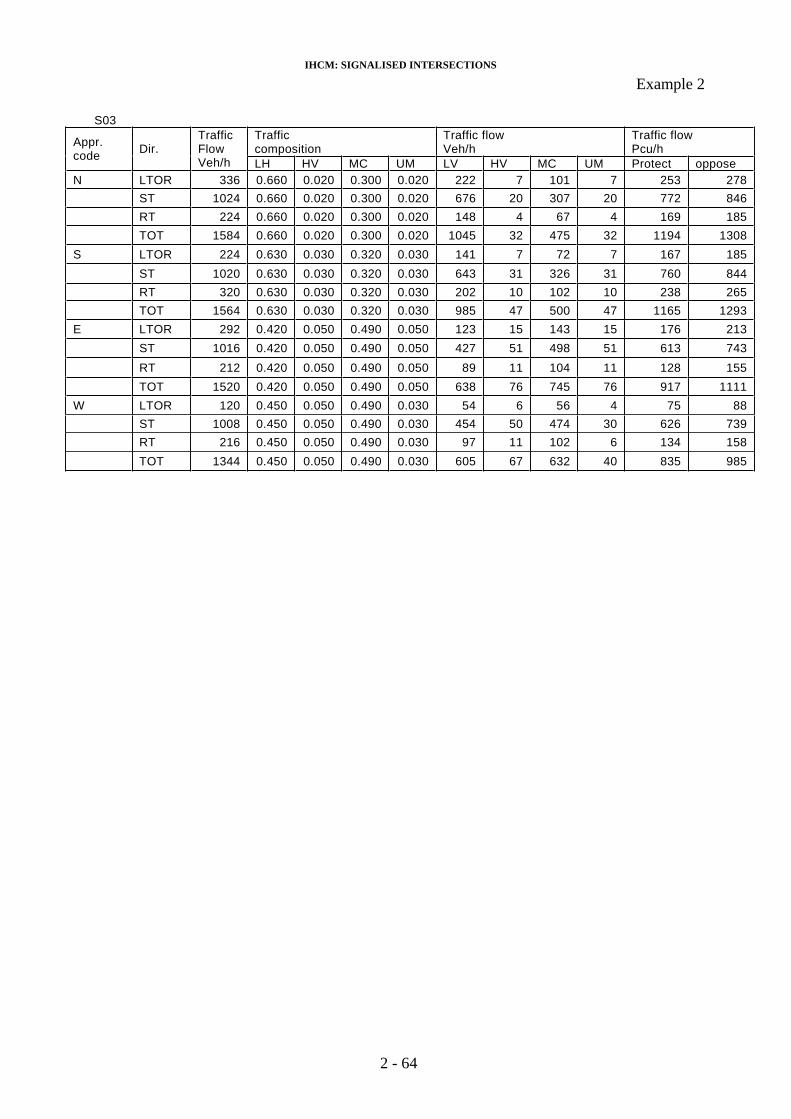
IHCM: SIGNALISED INTERSECTIONS
Example 2
S03Trafficcomposition
Traffic flowVeh/h
Traffic flowPcu/hAppr.
code Dir.TrafficFlowVeh/h LH HV MC UM LV HV MC UM Protect oppose
N LTOR 336 0.660 0.020 0.300 0.020 222 7 101 7 253 278ST 1024 0.660 0.020 0.300 0.020 676 20 307 20 772 846RT 224 0.660 0.020 0.300 0.020 148 4 67 4 169 185TOT 1584 0.660 0.020 0.300 0.020 1045 32 475 32 1194 1308
S LTOR 224 0.630 0.030 0.320 0.030 141 7 72 7 167 185ST 1020 0.630 0.030 0.320 0.030 643 31 326 31 760 844RT 320 0.630 0.030 0.320 0.030 202 10 102 10 238 265TOT 1564 0.630 0.030 0.320 0.030 985 47 500 47 1165 1293
E LTOR 292 0.420 0.050 0.490 0.050 123 15 143 15 176 213ST 1016 0.420 0.050 0.490 0.050 427 51 498 51 613 743RT 212 0.420 0.050 0.490 0.050 89 11 104 11 128 155TOT 1520 0.420 0.050 0.490 0.050 638 76 745 76 917 1111
W LTOR 120 0.450 0.050 0.490 0.030 54 6 56 4 75 88ST 1008 0.450 0.050 0.490 0.030 454 50 474 30 626 739RT 216 0.450 0.050 0.490 0.030 97 11 102 6 134 158TOT 1344 0.450 0.050 0.490 0.030 605 67 632 40 835 985
2 - 64

IHCM: SIGNALISED INTERSECTIONS
2 - 65
Example 2

IHCM: SIGNALISED INTERSECTIONS
2 - 66
Example 2

IHCM: SIGNALISED INTERSECTIONS
2 - 67
Example 2

IHCM: SIGNALISED INTERSECTIONS
2 - 68
Example 2
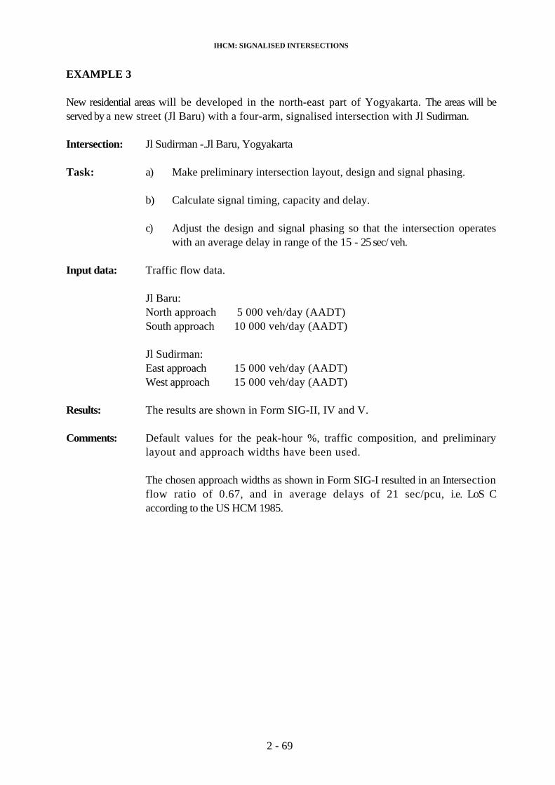
IHCM: SIGNALISED INTERSECTIONS
EXAMPLE 3
New residential areas will be developed in the north-east part of Yogyakarta. The areas will beserved by a new street (Jl Baru) with a four-arm, signalised intersection with Jl Sudirman.
Intersection: Jl Sudirman -.Jl Baru, Yogyakarta
Task: a) Make preliminary intersection layout, design and signal phasing.
b) Calculate signal timing, capacity and delay.
c) Adjust the design and signal phasing so that the intersection operates with an average delay in range of the 15 - 25 sec/ veh.
Input data: Traffic flow data.
Jl Baru:North approach 5 000 veh/day (AADT)South approach 10 000 veh/day (AADT)
Jl Sudirman:East approach 15 000 veh/day (AADT)West approach 15 000 veh/day (AADT)
Results: The results are shown in Form SIG-II, IV and V.
Comments: Default values for the peak-hour %, traffic composition, and preliminarylayout and approach widths have been used.
The chosen approach widths as shown in Form SIG-I resulted in an Intersectionflow ratio of 0.67, and in average delays of 21 sec/pcu, i.e. LoS Caccording to the US HCM 1985.
2 - 69

IHCM: SIGNALISED INTERSECTIONS
Example 3 INDONESIAN HIGHWAY CAPACITY MANUAL
Form SIG-I SIGNALISED INTERSECTION Date: 02 February 1993 Handled by: KLBForm SIG-I: GEOMETRY City: Yogyakarta
TRAFFIC CONTROL Intersection: Jl. Baru – Jl. SudirmanENVIRONMENT City size: 0.42 M
Case: aPeriod:
EXISTING SIGNAL PHASES
SITE CONDITIONSApproach witdh (m)
ApproachCode
(1)
RoadEnvironment
Type(2)
SideFriction
H/L(3)
MedianY/N
(4)
Gradient+/- %
(5)
Left-turn
On Red Y/N(6)
DistanceTo
parkedVehicle
(m)(7)
ApproachWA(6)
EntryWENTRY
(9)Exit
WEXIT(10)
N RES L N 0 N 4.5 4.5 4.5S RES L N 0 N 4.5 4.5 4.5E RA L Y 0 Y 7.0 7.0 6.0W RA L Y 0 Y 7.0 7.0 6.0
2 - 70

IHCM: SIGNALISED INTERSECTIONS
Example 3NEW
Trafficcomposition
Traffic flowVeh/h
Traffic flowPcu/hAppr.
code Dir.TrafficFlowVeh/h LH HV MC UM LV HV MC UM Protect oppose
N LT 74 0.340 0.030 0.490 0.140 25 2 36 10 39 53ST 352 0.340 0.030 0.490 0.140 120 11 172 49 188 252RT 74 0.340 0.030 0.490 0.140 25 2 36 10 39 53TOT 500 0.340 0.030 0.490 0.140 170 15 245 70 267 358
S LT 149 0.340 0.030 0.490 0.140 51 4 73 21 79 107ST 702 0.340 0.030 0.490 0.140 239 21 344 98 374 502RT 149 0.340 0.030 0.490 0.140 51 4 73 21 79 107TOT 1000 0.340 0.030 0.490 0.140 340 30 490 140 533 715
E LT 224 0.340 0.030 0.490 0.140 76 7 110 31 119 160ST 1052 0.340 0.030 0.490 0.140 358 32 515 147 561 752RT 224 0.340 0.030 0.490 0.140 76 7 110 31 119 160TOT 1500 0.340 0.030 0.490 0.140 510 45 735 210 800 1073
W LT 224 0.340 0.030 0.490 0.140 76 7 110 31 119 160ST 1052 0.340 0.030 0.490 0.140 358 32 515 147 561 752RT 224 0.340 0.030 0.490 0.140 76 7 110 31 119 160TOT 1500 0.340 0.030 0.490 0.140 510 45 735 210 800 1073
2 - 71
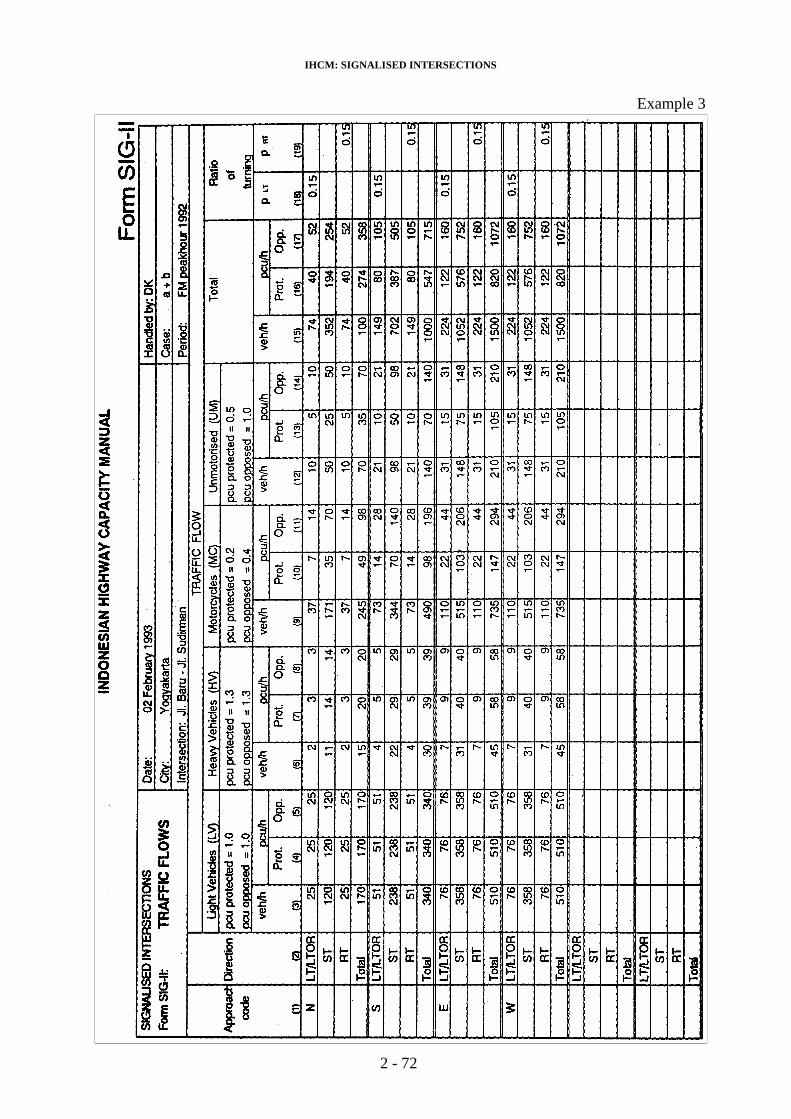
IHCM: SIGNALISED INTERSECTIONS
Example 3
2 - 72

IHCM: SIGNALISED INTERSECTIONS
Example 3
2 - 73
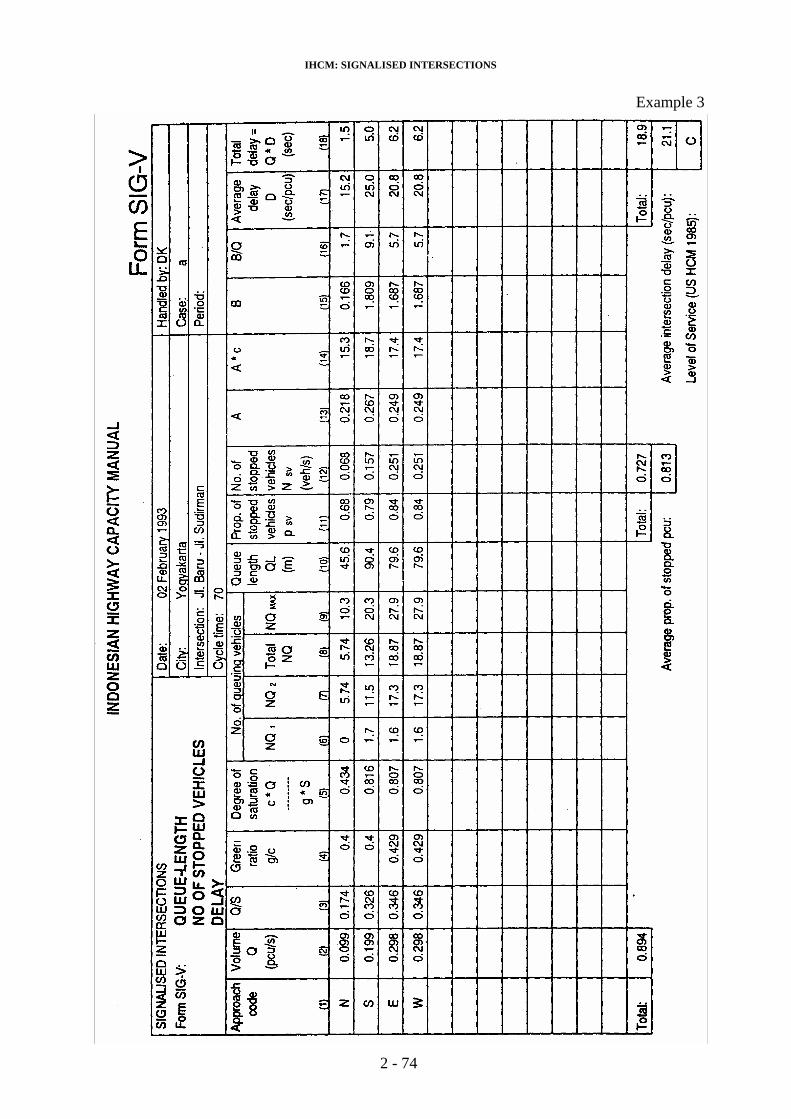
IHCM: SIGNALISED INTERSECTIONS
Example 3
2 - 74

IHCM: SIGNALISED INTERSECTIONS
5 LITERATURE REFERENCES
S1. TRB Highway Capacity Manual.Transportation Research Board Special Report 209; Washington D.C. USA 1985.
S2. Bang, Karl-L. Swedish Capacity Manual Part 3: Capacity of SignalizedIntersections.Transportation Research Record 667; Washington D.C. USA 1978.
S3. Webster, F.V. Traffic signals.Cobbe, B.M. Roads Research Laboratory, Technical Paper No. 56.
Crowthorne, Berkshire U.K. 1966.
S4. Akcelik, R. Traffic signals; Capacity and Timing Analysis. AustralianRoad Research Board. Report No. 123; Vermont South, Victoria, Australia 1989.
S5. May, A.D. Comparative Analysis of Signalized Gedizlioglu, E. Intersection Capacity Methods. Tai, L. Transportation Research Record 905;
Washington D.C. USA 1983.
S6. Rois, H. Effect of Motorcycles in Signalised Intersections. Thesis ITBS2 STJR, Bandung Indonesia 1992.
2 - 75

IHCM: SIGNALISED INTERSECTIONS
Appendix 2:1INDONESIAN HIGHWAY CAPACITY MANUAL
Form SIG-I SIGNALISED INTERSECTION Date: Handled by:Form SIG-I: GEOMETRY City:
TRAFFIC CONTROL Intersection:ENVIRONMENT City size:
Case:Period:
EXISTING SIGNAL PHASES
SITE CONDITIONSApproach witdh (m)
ApproachCode
(1)
RoadEnvironment
Type(2)
SideFriction
H/L(3)
MedianY/N
(4)
Gradient+/- %
(5)
Left-turnOn Red
Y/N(6)
DistanceTo
parkedVehicle
(m)(7)
ApproachWA(6)
EntryWENTRY
(9)Exit
WEXIT(10)
2 - 76

IHCM: SIGNALISED INTERSECTIONS
Appendix 2:1
2 - 77

IHCM: SIGNALISED INTERSECTIONS
Appendix 2:1INDONESIAN HIGHWAY CAPACITY MANUAL
Form SIG-III SIGNALISED INTERSECTIONS Date:
Form SIG-III: CLEARENCE TIME Handled by:
LOST TIME City:
Intersection:
Case:
EVACUATING TRAFFIC ADVANCING TRAFFICClearance
Time(sec)
ApproachApproach
Speed
V E m/sec Speed V A m/sec
Distance evac-adv (m)*)
Time evac-adv (sec)**)
Distance evac-adv (m)*)
Time evac-adv (sec)**)
Distance evac-adv (m)*)
Time evac-adv (sec)**)
Distance evac-adv (m)*)
Time evac-adv (sec)**)
Distance evac-adv (m)*)
Time evac-adv (sec)**)
Distance evac-adv (m)*)
Time evac-adv (sec)**)
Dimensioning clearance time (=allred)
Phase 1 Phase 2
Phase 2 Phase 3Phase 3 Phase 1
Phase Phase
Total amber time (3 sec/phase)
Total lost time (LT) = Total all red + amber time (sec/cycle)
*) From drawing, see example Figure B-2:1**) Time for evacuation = (LEV+IEV)/VEV Time for advancement = LAV/VAV
2 - 78

IHCM: SIGNALISED INTERSECTIONS
Appendix 2:1
2 - 79

IHCM: SIGNALISED INTERSECTIONS
2 - 80
Appendix 2:1

Chapter 3 : UNSIGNALISED INTERSECTIONS

IHCM: UNSIGNALISED INTERSECTION
CHAPTER 3
UNSIGNALISED INTERSECTIONS
TABLE OF CONTENTS
1. INTRODUCTION ............................................................................................3 – 2
1.1 SCOPE AND OBJECTIVES ..................................................................................3 – 21.2 DEFINITIONS AND TERMINOLOGY ............................................................3 – 3
2. METHODOLOGY ……………………...………...…………………………3 – 9
2.1 GENERAL PRINCIPLES ....................................................................................3 – 92.2 OVERVIEW OF CALCULATION PROCEDURE .............................................3 – 112.. 3 GUIDELINES FOR APPLICATION ..................................................................3 – 12
3. CALCULATION PROCEDURE .....................................................................3 – 13
STEP A: INPUT DATA .............................................................................3 – 13A-1: Geometric conditions .............................................................3 – 13
A-2: Environmental conditions .......................................................3 – 16 A-3: Traffic conditions ..................................................................3 – 17STEPB: DESIGN /PLANNING -OBJECTIVES ...........................................3 – 21STEP C: CAPACITY C .............................................................................3 – 22
C-1: Base capacity value Co .......................................................................................... 3 – 23C-2: Entry width correction factor FW ...................................................................3 – 23C-3: Major road median correction factor FM ...................................................3 – 24C-4: City size correction factor FCS ........................................................................... 3 – 24C-5: Road environment type and side friction
correction factor FRI ..............................................................3 – 24C-6: Left-turning-% correction factor FLT ............................................................3 – 25C-7: Right-turning-% correction factor FRT ........................................................ 3 – 26C-8: Split correction factor F5 ........................................................................................ 3 – 27C-9: Actual capacity C ..................................................................3 – 27
STEP D: DEGREE OF SATURATION DS ..................................................3 – 28STEP E: DELAY D ....................................................................................3 – 29STEPF: QUEUE PROBABILITY QP% ......................................................3 – 30STEP G: PERFORMANCE MEASURES COMPARED WITH
DESIGN/PLANNING OBJECTIVES ...........................................3 – 31
4. WORKED EXAMPLES .....................................................................................3 – 32
5. LITERATURE REFERENCES ...........................................................................3 – 38
Appendix 3:1 CALCULATION FORM ………………………...…...…….. 3 – 39
3 - 1

IHCM: UNSIGNALISED INTERSECTION
1 . INTRODUCTION
1.1 SCOPEAND OBJECTIVES
This Chapter deals with 3-way and 4-way unsignalised intersections (definition see Section1.2), which are formally controlled by the basic Indonesian traffic code rule give-way to the left.
The following performance measures can be estimated for given conditions regardinggeometry, environment and traffic with the method outlined in this chapter:- Capacity - Degree of saturation- Delay- Queue probabilityThese measures are defined in Chapter 1 Section 4 "General definitions and terminology".Since the methods described in this manual are empirical, the results should always be madesubject to a qualified traffic engineering judgement. This is especially important if the method isused outside the range of variation for the variables in the empirical data base. This range isshown in Table 1.1:1.
4-way 3-wayVariable
Min. Avg Max. Min. Avg Max.Entry width 3.5 5.4 9.1 3.5 4.9 7.0Left- turning-% 10 17 29 6 26 50Right-turning-% 0 13 26 9 29 51
Split-% 27 38 50 15 29 41
Light vehicle-%o 29 56 75 34 56 78
Heavy vehicle-% 1 3 7 1 5 10
Motor cycle-% 19 33 67 15 32 54
Unmotorised-% 1 8 22 1 7 25
Table 1.1:1 Range of variation in empirical data for input variables The method assumesright angled intersections in flat terrain.
The method estimates the expected impact of the influencing variables based on the empirical datacollected. Used on the data from which it is derived the error of the capacity estimate isnormally less than ± 20%.
The method is valid for degree of saturation less than 0.8-0.9. At higher traffic demands trafficbehaviour becomes more aggressive and there is a major risk that the intersection gets blockedby drivers competing for the limited space in the conflict zone.
The method is derived from sites, which are operating with average Indonesian traffic behaviour. If this behaviour changes, for instance through implementation and enforcement
3 - 2

IHCM: UNSIGNALISED INTERSECTION
of STOP- or YIELD-sign control in unsignalised intersections, or through an enforcementof the formal traffic code rules, the method would be less valid.
1.2 DEFINITIONS AND TERMINOLOGY
Notations, terminology and definitions used especially for unsignalised intersections are listed below. General definitions, e.g. for performance measures, are given in Chapter 1, Section 4.
Geometric conditions
NOTATION TERMINOLOGY DEFINITION
3-WAY AND 4-WAYINTERSECTION
Intersection with 3 arms and 4-armsrespectively.
Figure 1.2:1 3-and 4-way intersection
MAJOR/MINOR ROAD The major road is the most important road in the intersection, e.g. in terms of road classification.In 3-way intersections the continuous road isalways defined as the major road.
A,B,C,D APPROACH Area for entering vehicles in an intersection arm.Major road approaches are denoted B and D,minor A and C giving a clockwise order.
MAJOR ROAD MEDIANTYPE
Classification of major road median typedepending on possibility to use the median topass the major road in two steps.
Wx ENTRY WIDTH FORAPPROACH X (m)
Width of the paved part of the approach,measured at the bottleneck, used by movingtraffic. X denotes approach identification. If theapproach is extensively used for parking,2m should be deducted from the physical width.
3 - 3

IHCM: UNSIGNALISED INTERSECTION
WE INTERSECTIONENTRY WITDH (m)
Average effective witdh for all approaches with entering traffic.
WAC ROAD ENTRY WITDH (m)
Average witdh of the approach(es) to anintersection from one road.
WBD INTERSECTION TYPE Code for number of intersection arms andnumber of lanes on minor and major road in the intersection.
IT NUMBER OF LANES Number of lanes defined from the road entry widths of the road, see Figure 1.2:2
Road entry width, WAc, WBD
(m)No. of lanes. (total for both directions)
WBD = (b + d/2)/2 < 5.5 2WAC = (a/2 + c/2)/2 > 5.5 4
Figure 1.2:2 Determination of number of lanes
Environmental conditions See definitions in Chapter 1, Section 4.
Traffic conditions
LT LEFT-TURNING Index for left-turning traffic.
ST STRAIGHT-THROUGH Index for straight-through traffic.
RT RIGHT-TURNING Index for right-turning traffic.
Qv TOTAL ACTUAL FLOW(veh / h)
Total incoming flow to the intersection (veh/h).
Qp TOTAL ACTUAL FLOW(pcu/h)
Total incoming flow to the intersection(pcu/h).
QMA TOTAL MAJOR ROAD FLOW
Total incoming flow from major road (veh/h orpcu / h).
QMI TOTAL MINOR ROADFLOW
Total incoming flow from minor road (veh/h or pcu/h).
3 - 4

IHCM: UNSIGNALISED INTERSECTION
SP% ROAD FLOW SPLIT-% % minor road flow of total incoming flow(based on calculation in veh/h).
LV% LIGHT VEHICLE-% % Light vehicles of all vehicles entering theintersection.
HV% HEAVY VEHICLE-% % Heavy vehicles of all vehicles entering theintersection.
MC% MOTOR CYCLE-% % Motor cycles of all vehicles entering theintersection.
UM% UNMOTORISED-% % Unmotorised vehicles of all vehicles enteringthe intersection.
P PCU-FACTOR Factor to convert a flow expressed in veh/h intopcu /h.
K AADT-FACTOR Conversion factor from AADT to peak hour traffic.
Calculation factors: NOTATION TERMINOLOGY DEFINITION
C0 BASE CAPACITY(pcu/h)
Capacity for an intersection type for a pre-determined ('base") set of influencing conditions.
FW ENTRY WIDTHCORRECTION FACTOR
Correction factor for base capacity due tointersection entry width.
FM MAJOR ROAD MEDIAN TYPE CORRECTIONFACTOR
Correction factor for base capacity due to majorroad median type.
FCS CITY SIZE CORRECTION FACTOR
Correction factor for base capacity due to citysize.
.FRF ROAD ENVIRONMENT TYPE AND SIDE FRICTION CORRECTIONFACTOR
Correction factor for base capacity due to road environment type and side friction level.
FLT LEFT-TURNINGCORRECTION. FACTOR
Correction factor for base capacity due to leftturning%.
FRT RIGHT-TURNINGCORRECTION FACTOR
Correction factor for base capacity due to rightturning%.
3 - 5

IHCM: UNSIGNALISED INTERSECTION
FN ROAD FLOW SPLITCORRECTION FACTOR
Correction factor for base capacity due to road flow split-%.
3 - 6

IHCM: UNSIGNALISED INTERSECTION
Typical conflicts at an unsignalised intersection in Bandung
3 - 7

IHCM: UNSIGNALISED INTERSECTION
Unsignalisedfour-armintersection in Palembang
Unsignalisedfour-armintersection in Ujung Pandang
Right-of-wayfrom the left isgenerally not respected inunsignalisedintersection
3 - 8

IHCM: UNSIGNALISED INTERSECTION
2. METHODOLOGY
2.1 GENERAL PRINCIPLES
The method and procedures described in this manual have an empirical basis. The reason. for this isthat the Indonesian traffic behaviour in unsignalised intersections in terms of give-way rules, lanediscipline and queuing rules are very difficult to describe in an explanatory, behavioural model such as gap-acceptance based stop/give way models. The driver behaviour is entirely differentfrom what is found in most Western countries, which makes the adoption of methods fromWestern capacity manuals impossible. The most decisive results for traffic behaviour are on average almost two thirds of all crossing vehicles from minor road pass the intersection in non-gapping behaviour, and the critical gap for the vehicles that do not pass by "force" is verylow (around 2 seconds).
The method estimates the impact on capacity and other related measures from site conditions regarding geometry, environment and traffic demand.
a) Capacity_
The total capacity for all arms of the intersection is calculated as the product between a basecapacity (C0) for a set of predetermined (ideal) conditions and correction factors (F), takingaccount of the influence on capacity of the actual site conditions.
The format of the capacity model is thus as follows:
C= C0 x FW x FM x FCS x FRF x FLT x FRT x FSP
The input variables for estimation of capacity C (pcu/h) by use of the model are as follows:
Variable type Variable description and input name
Modelfactor
Geometry Intersection typeIntersection entry width Major road median type
ITWE
MFW
FMEnvironment City size class
Road environment and side friction class
CS
RF
FCS
FRF
Traffic Left-turning-%Right-turning-%Road flow split-%
LT%RT%SP%
FLT
FRT
FSP
Table 2.1:1 Overview of capacity model input variables
In some western manuals the angle in skew intersection has an effect on capacity. TheIndonesian manuals is not based on gap-acceptable methods, and there is no clear distinction
3 - 9

IHCM: UNSIGNALISED INTERSECTION
between major and minor road. Since the Manual also does not enable calculation of approach capacity but intersection capacity, the turn angle of the approach is not used.
b) Degree of saturation
Degree of saturation for the whole intersection, DS, is calculated as:
DS = QP/C,whereQp Total actual flow (pcu/h) is calculated as follows: Qp = Qv x PP The pcu-factor, calculated as follows:
P = (pcuLVx LV% + pcuHV x HV% + pcuMC x MC%o + pcuMC x UM%) / 100 where pcuLV LV%, pcuHV, HV%, pcuMC, MC% and pcuMC, UM% are pcu-
values and %-flow for light vehicles, heavy vehicles, motor cycles and unmotorised vehicles.
C Capacity (pcu/h)
c) Delay D
Average delay for the whole intersection (sec/pcu) is estimated from an empirically based delay/degree of saturation curve. Delay increases significantly with total flow, simultaneous-ly with major and minor flow and with degree of saturation. The results obtained from observations showed that there is no gapping behaviour at high flows. This means that Western models for stop/give-way behaviour of the traffic from the minor road are notapplicable. The maximum stable outflow at predefined conditions is very difficult to define,since the variance in behaviour and outflow is enormous. Instead capacity has been defined as the total intersection flow when the average delay per vehicle exceeds apredefined value considered high, 15 seconds. Delay values from this method can be used together with delay and travel time values from methods for other types of trafficfacilities described in this manual in order to estimate travel times along routes in networks.
d ) Queue probability QP%
Queue probability QP% (%) is estimated from an empirically based queue probability/degree of saturation curve.
3 - 10

IHCM: UNSIGNALISED INTERSECTION
2.2 OVERVIEW OF CALCULATION PROCEDURE
Capacity (C) and the performance measures Degree of saturation DS, Delay D (sec/pcu) and Queue probability QP% are calculated for given geometric, environmental and traffic conditions as follows, see Figure 2.2:1.
Figure 2.2:1 Overview of the calculation procedure.
Recording of the input data as well as of the results from the calculations can be done in Form UNSIG-I (Appendix 3:1). The form is divided into four main parts: GEOMETRY,TRAFFIC, ENVIRONMENT and ANALYSIS. In GEOMETRY an overview sketch ofthe intersection is drawn and geometric conditions are entered. In TRAFFIC the design trafficsituation is visualised and traffic input conditions are recorded. In ENVIRONMENT,environmental conditions are entered. In ANALYSIS the results from the different calculation stepsare documented. Each column in the ANALYSIS part has an identifier, which is used in theexplanation of how to enter data into the form.
3 - 11

IHCM: UNSIGNALISED INTERSECTION
2.3 GUIDELINES FOR APPLICATION
This Highway capacity manual can be used for many different applications such as design,planning and operational analysis.
The purpose of design is to find suitable layout and geometric dimensions which meets definedobjectives for the design traffic conditions. The method is used as follows, see Figure 2.3:1.
Figure 2.3:1 Overview of the calculation procedure for design, planning and operational analysis
Planning differs from design only in time scale. In the design application, the input traffic data normally relate to a peak hour. In planning, traffic data information is usually in theform of a predicted AADT, which then has to be converted to a design peak hour, normallyby using a default percentage factor.
Operational analysis normally is done with the purpose to estimate intersection performancemeasures for a specified lay-out, environmental and traffic situation.
3 - 12

IHCM: UNSIGNALISED INTERSECTION
3. CALCULATION PROCEDURE
STEP A: INPUT DATA
STEP A-1: GEOMETRIC CONDITIONS
Overview sketch
Normally a sketch of the geometric layout is drawn in Form UNSIG-I, see example belowinFigure A-1:1. Minor and major road names and city name are noted in the head of the sketch as well as an optional name of the design alternative. The sketch should give a good overview of the intersection with information on kerbs, carriageway, shoulder and median widths. For orientation it should also contain a directional arrow.
Major road is the road which is considered to be of most importance in the intersection, e.g. the road with the highest functional classification. For 3-way intersections the continuous road is always the major road.
The minor road approaches should be denoted A and C. The major road approaches shouldbe denoted B and D. The notation should be made in a clock-wise order.
Figure A-1:1 Example of geometric input data sketch.
3 - 13

IHCM: UNSIGNALISED INTERSECTION
Geometric input conditions
The following geometric input data is needed for the capacity analysis, and should be recorded in the geometry part of the form.
a) Road entry widths WAC, WBD and Intersection entry width WE.
Enter the individual approach widths and calculate average Road entry widths and Intersectionentry width. The individual approach width is measured at 10 m distance from theimaginary line connecting the edge of pavement of the crossing road. Road entry widths for minorroad WAC and major road WBD are the average approach widths for minor and major road.Intersection entry width, WE (m) is the average effective entry width for approaches withpermitted entering traffic, see Figure A-1:2.
For approaches, where the entry is frequently used for parking at distance less than 20 m from the imaginary line connecting edge of pavement of the crossing road, 2m should be subtracted from the approach entry width.
Intersection entry width (approach average), WE
WE = (a/2 + b + c/2 + d/2)/4
If A is only exit:
WE = (b + c/2 + d/2)/3
Road entry widths
WAC = (a + c)/2 WBD = (b + d/2)/2
Figure A-1:2 Road entry withds WAC, WBD and Intersection entry width WE
b) Intersection type
Intersection type defines number of intersection arms and number of lanes on minor andmajor road in the intersection by a three digit code, see Table A-1:1.
I T code
No. of inter- section arms
No. of minorroad lanes
No. of majorroad lanes
322 3 2 2324 3 2 4342 3 4 2422 4 2 2
424 4 2 4Table A-1:1 Intersection type code
3 - 14

IHCM: UNSIGNALISED INTERSECTION
The number of arms is the number of arms with either entering or exiting traffic, or both.
The number of lanes is defined from the average Intersection entry width for the roads,WE, as follows, see Figure A-1:3.
Road entry width, WAc, WBD
(m)No. of lanes. (total for both directions)
WBD = (b + d/2)/2 < 5.5 2WAC = (a/2 + c/2)/2 > 5.5 4
Figure A-1:3 Number of lanes and road entry witdh WE
Maior road median type M
The major road should be classified by median type, if the major road is 4-lane, as follows, see Table A-1:2.
Type M Description
NoneNarrowWide
No major road median.Major road median exists, but does not allow passage in two steps. Major road median exists and allows passage in two steps.
Table A-1:2 Major road median types.
Traffic engineering judgement is needed to decide the median factor. The median is wide if astandard light vehicle can shelter in the median area without disturbing the discharge of trafficon the major road. This is possible if the median is 4m or wider. In some cases, e.g if the majorroad approaches are wide, this might occur at more narrow medians.
3 - 15

IHCM: UNSIGNALISED INTERSECTION
STEP A-2: ENVIRONMENTAL CONDITIONS
The following environmental data is needed for calculation and should be filled in theenvironment part of the form.
a) Road environment type RE
The road environment should be classified by type. Road environment type classes describe landuse and accessibility of the roads from surrounding activities. It is defined qualitatively from traffic engineering judgement:
Commercial Commercial landuse (e.g. shops, restaurants, offices) with direct roadside access for pedestrians and vehicles.
Residential Residential landuse with direct road side access for pedestrians and vehicles.
Restrictedaccess
No or limited direct roadside access (e.g. due to the existence ofphysical barriers, frontage streets etc).
Table A-21 Road environment type classes.
c) Side friction class SF
Side friction describes the impact of road side activities in the intersection area on the traffic discharge,e.g. pedestrians walking on or crossing the carriageway, angkutan kota and buses stopping to pick up or let off passengers, vehicles entering and leaving premises and parking lots outside the carriageway. Sidefriction is defined qualitatively from traffic engineering judgement as High or Low
d) City size class CS
The city size should be classified by the population of the whole urban area.
CS No. of inhabitants (M)
Small <0.3Medium 0.3 - 1.0
Large 1.0 - 3.0
Very large > 3.0
Table A-2:2 City size classes
3 - 16

IHCM: UNSIGNALISED INTERSECTION
STEP A-3: TRAFFIC CONDITIONS
The input data on traffic conditions consists of three parts, definition of the traffic situation, a trafficflow sketch and traffic input variables.
The traffic flow sketch is optional and gives more detailed traffic information than what is needed for the analysis of unsignalised intersections. If the alternative to signalise theintersection is also to be tested, this information is however needed.
Traffic situation
The traffic situation is defined by year and hour or AADT-factor (for planning). An optional nameof the traffic alternative could be entered.
Traffic flow sketch - optional
For design and operational analysis a sketch of the traffic situation could be drawn in Form UNSIG-l. The sketch should show traffic movements (veh/h) by approach ALT, AST, ART and soon. Flow dimension, veh/h or AADT, is marked in the form.
Figure A-3:1 Example traffic flow sketch
3 - 17

IHCM: UNSIGNALISED INTERSECTION
Traffic input variables
The following traffic data are needed for the calculation and should be filled in the trafficpart of the form, see also Figure A-3:2
Figure A-3:2 Traffic flow variables
The variables are described below in 'the order they appear in the UNSIG-I form.
COLUMN IN FORM COMMENT
Traffic flows Defines if flows are in veh/h or AADT.
AADT-factor K The total flow is given as an AADT-value QAADT AADT-factor, K, is a conversion factor to estimate an average peak hour traffic from an AADT, as follows. Qpeak = K X
QAADT The following default values could be used if no better information is available:
K-factor - City sizeRoad environment
>1M <1MRoads in commercial areas and arterial roads
0.07-0.08 0.08-0.10
Roads in residential areas 0.08-0.09 0.09-0.12
Table A-3:1 K-factor default values
Minor road traffic (veh/h) Total entering traffic QMI from minor road. For split-% calcula-tion.
3 - 18

IHCM: UNSIGNALISED INTERSECTION
Major road traffic (veh/h) Total entering traffic QMA from major road. For total traffic cal-culation.
Left turning Total left turning traffic.traffic QLT (veh/h) For LT%-calculation.
Right turning Total right turning traffic.traffic QRT (veh/h) For RT%-calculation.
Total traffic Total entering traffic.Qv (veh / h)
Left turning-% LT% Left-turning-%, LT%, is the overall left-turning-% LT%=100xQLT/Qv for the intersection calculated for veh/h.
Right turning-% RT% Right-turning-%, RT%, is the total right-turning-%RT%=100 x QRT/Qv for the intersection calculated for veh/h.
Road flow split-% Road flow split-%, SP% is the % minor road traffic ofSP%=100xQMI/Qv total incoming traffic calculated for veh/h.
PCULV pcu-factor for light vehicles. Default: PC.ULV=1.0.
LV% %a-light vehicles of total flow, LV%
PcuHV pcu-factor for heavy vehicles. Default: pcuHV=1.3. Comment:If there are a lot of heavy trucks PCUHV =2.0 could be used.
HV% %-heavy vehicles of total flow, HV%
PCUMC pcu-factor for motor cycles. Default: pcuMc=0.5.
MC% %-motor cycles of total flow, MC%
PcuUM pcu-factor for unmotorised vehicles. Default: pcuu,,,,=1.0. Comment: If most unmotorised are bicycles pcuUM=0.3 could be used.
UM% %-unmotorised of total flow UM%
Pcu-factor P P is calculated from pcu-values and flow composition data:
P = (pcuLV x LV% + PCUHV x HV% + pcuMc x MC% + pcuMc x UM%) / 100 Normally the default pcu-values for the different vehicletypes are used.
3 - 19

IHCM: UNSIGNALISED INTERSECTION
Total traffic QP (pcu/h) Total flow QP (pcu/h) is calculated as follows:
QP = Qv x P, where
Qv = total entering flow (veh/h)P = pcu-factor
Example: Qv = 2000 veh/h withLV HV MC UM
pcu % pcu % pcu % pcu %
1.0 56 1.3 4 0.5 33 1.0 7 Solution:
P = (1.0x56+1.3x4+0.5x33+1.0x7) / 100 = 0.85
Qp = PxQv = 0.85x2000 = 1700 pcu/h
Traffic variable default values
Traffic data is often lacking or of poor quality. The following default values could be used if better information is not available, see Table C-1:2, for AADT-factor K, road flow splitSP%, left-turning-% LT%, right turning-% RT%, composition P-factor and vehidepercentages.
Factor Default
AADT-factor, see Table C-1:1, K 0.07-0.12Split-%, SP% 25
Left turning-%, LT% 15
Right turning-%, RT% 15
Pcu-factor, P 0.85
Traffic composition % City size M inhabitants LV HV MC UM
< 0.3 60.0 2.5 33.0 4.5
0.3 – 1.0 34.0 3.0 49.0 14.0
1.0-3.0 52.5 3.5 39.0 5.0
> 3.0 59.0 4.5 35.5 1.0
Table A-3:2 Default traffic variable
3 - 20

IHCM: UNSIGNALISED INTERSECTION
STEP B: DESIGN /PLANNING OBJECTIVES
For design/planning calculations, objectives expressed in performance measures must bechosen.A recommended default objective for design/planning is to find a design which operates with degree ofsaturation DS<=O.8
Chosen objectives are entered into the UNSIG-I form in the OBJECTIVES-part.
3 - 21
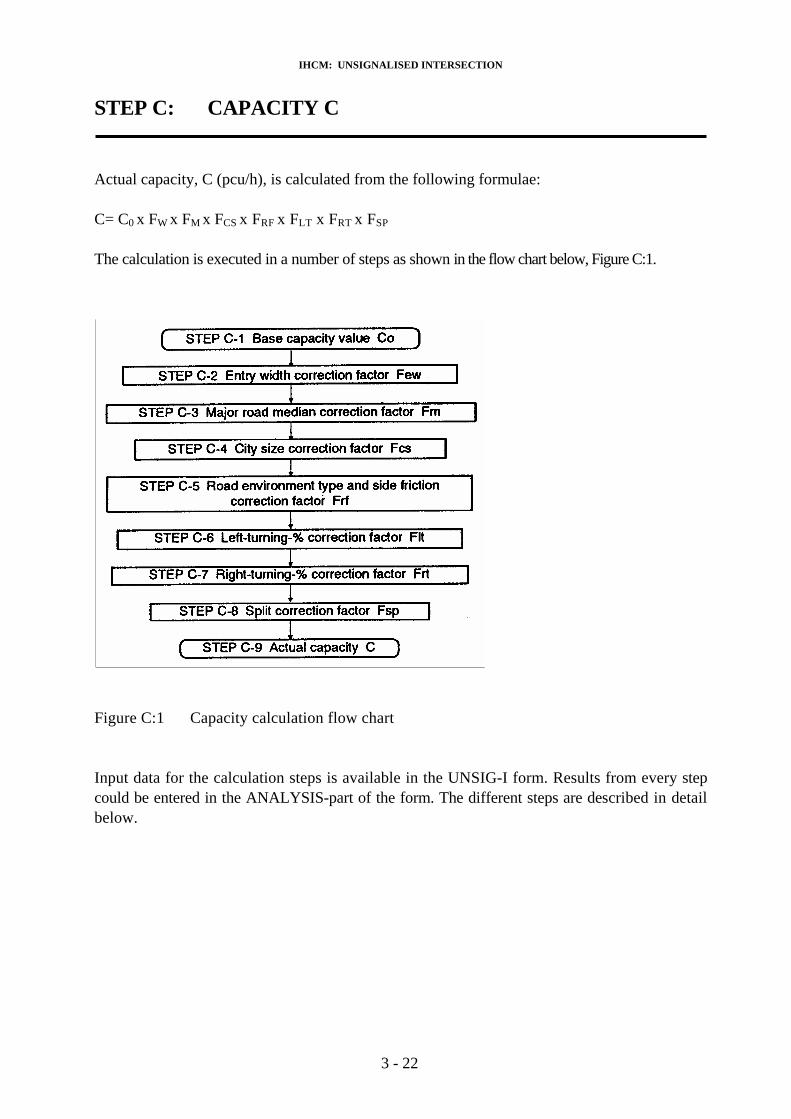
IHCM: UNSIGNALISED INTERSECTION
STEP C: CAPACITY C
Actual capacity, C (pcu/h), is calculated from the following formulae:
C= C0 x FW x FM x FCS x FRF x FLT x FRT x FSP
The calculation is executed in a number of steps as shown in the flow chart below, Figure C:1.
Figure C:1 Capacity calculation flow chart
Input data for the calculation steps is available in the UNSIG-I form. Results from every stepcould be entered in the ANALYSIS-part of the form. The different steps are described in detailbelow.
3 - 22

IHCM: UNSIGNALISED INTERSECTION
STEP C-1: BASE CAPACITY VALUE C0
Base capacity value C0 is taken from Table C-1:1 and is recorded in Column C-1 in theANALYSIS part of the form.Input variable is intersection type IT.
Intersection type IT Base capacity C0 (pcu/h)
322 2700
342 2900
324 3200
422 2900
424 3400
Table C-1:1 Intersection type base capacity C0 (pcu / h)
STEP C-2: ENTRY WIDTH CORRECTION FACTOR FW
The entry width correction, FW , is estimated from Figure C-2:1, and is recorded in Column C-2in the ANALYSIS-part of the form.
Input variables are intersection entry width WE and intersection type IT.
The range given in the figure is the range for the empirical base of the manual.
Figure C-2:1 Entry witdh correction factor FW
3 - 23

IHCM: UNSIGNALISED INTERSECTION
STEP C-3: MAJOR ROAD MEDIAN CORRECTION FACTOR FM
The major road median correction factor FM is estimated using Table C-3:1. The result is enteredin Column C-3 in the ANALYSIS-part of the form. The correction should only be used for 4-lane major roads! Input variable is major road median type.
Major road median type
Median correction factor, FM
None 1.0Narrow 1.0Wide 1.2
Table C-3:1 Major road median correction factor FM
STEP C-4: CITY SIZE CORRECTION FACTOR Fcs
City size correction factor FOE is decided from Table C-4:1. The result is entered in Column C-4 in the ANALYSIS-part of the form. Input variable is city size, CS.
City size CS
Inhab. (M) City size correctionfactors FCS
Small < 0.3 0.83Medium 0.3-1.0 0.94
Large 1.0-3.0 1.00
Very large > 3.0 1.05
Table C-4:1 City size correction factor FCS
STEP C-5: ROAD ENVIRONMENT TYPE AND SIDE FRICTION CORRECTION FACTOR FRF
Road environment type and side friction correction, FRR is calculated using Table C-5:1 below,and the result is recorded Column C-5 in the ANALYSIS-part of the form. Input variables areroad environment type RE and side friction class SF.
Side frict on class SFRoad environmenttype class RE Low HighCommercial 1.00 0.94Residential 1.00 0.97Restricted access 1.00 1.00
Table C-5:1 Road environment type and side friction correction factor FRF
3 - 24

IHCM: UNSIGNALISED INTERSECTION
STEP C-6: LEFT-TURNING CORRECTION FACTOR FLT
Left-turning correction factor FLT is estimated from Figure C-6:1 below.
Input variable is left-turning-%, LT %.
The range given for LT% is the range for the empirical base of the manual.
Figure C-6:1 Left-turning correction factor FLT
3 - 25

IHCM: UNSIGNALISED INTERSECTION
STEP C-7: RIGHT-TURNING-% CORRECTION FACTOR FRT
Right-turning-% correction, FRT, is estimated from Figure C-7:1 below for 3-way intersections.
Input variable is right-turning-%, RT%.
The range given for RT% in the figure is the range for the empirical base of the manual.
For 4-way intersections FRT=1.0
Figure C-7:1 Right-turning-% correction factor FRT
3 - 26

IHCM: UNSIGNALISED INTERSECTION
STEP C-8: SPLIT CORRECTION FACTOR FSP
Split correction factor FSP is estimated from Figure C-8:1 below.
Input variables are road flow split-% and intersection type IT. The range noted "empirical data" for SP% in the figure is the range for the empirical base ofthe manual.
Figure C-8:1 split correction factor FSP
STEP C-9: ACTUAL CAPACITY C (pcu/h)
Actual capacity, C (pcu/h), is calculated using the following formulae, where the different factorshave been calculated above:
C= Co x FW x FM x FCS x FRF x FLT x FRT x FSP
3 - 27

IHCM: UNSIGNALISED INTERSECTION
STEP D: DEGREE OF SATURATION DS
Degsee of saturation, DS, is calculated using the fold formulae. The result is noted in the ANALYSIS-part of the form inColumn D:
DS= QP / C, where
QP Actual total flow (pcu/ h) from traffic input.
P pcu-factor from traffic input.
C Actual capacity from STEP C.
Example : C = 2700 pcu / h and Qv = 2000 veh / h with
LV HV MC UM
pcu % pcu % pcu % pcu %
1.0 56 1.3 4 0.5 33 1.0 7
Calculations:
P = (1.0 x 56+ 1.3 x 4 + 0.5 x 33 +1.0 x 7)/ 100 = 0.8.5
QP = P x QV = 0.85 x 2000 = 1700 pcu / h
Degree of saturation DS = QP / C = 1700 / 2700 = 0.63
3 - 28

IHCM: UNSIGNALISED INTERSECTION
STEP E: DELAY D
Delay D (sec/pcu) is average delay per entering vehicle. Delay is estimated from the empirical relationship between delay D and degree of saturation DS, see Figure E:1.
Input variable is degree of saturation DS from STEP D.
The result is noted in the ANALYSIS-part of the form in Column E.
Figure E:1 Delay D (sec/pcu) versus degree of saturation DS = QP / C
3 - 29

IHCM: UNSIGNALISED INTERSECTION
STEP F: QUEUE PROBABILITY QP %
A range of queue probability QP% (%) is estimated from the empirical relationshipbetween queue probability QP% and degree of saturation DS.
Input variable is degree of saturation DS from STEP D.
The result is noted in the ANALYSIS-part of the form in Column F.
Figure F:1 Range of queue probability QP % (%) versus degree of saturation DS = QP / C
3 - 30

IHCM: UNSIGNALISED INTERSECTION
STEP G: PERFORMANCE MEASURES COMPARED WITH DESIGN/PLANNING OBJECTIVES.
This step comprises the following sub-steps:
a) Compare calculated performance measures with design/planning objectives
b) If not satisfying, assume a new design and repeat calculations.
In some cases the objectives cannot be met. the objectives and/or traffic conditions thenhave to be changed.
Traffic can be changed by the introduction of turning regulations for some movements, or through alternative traffic schemes.
c) If satisfying, stop calculations.
The COMMENT-lines in the form UNSIG-I could be used for STEP G.
3 - 31

IHCM: UNSIGNALISED INTERSECTION
4. WORKED EXAMPLES
EXAMPLE
Determine capacity, degree of saturation, delay and queue probability for the unsignalised intersectionbetween Jalan BD and Jalan AC with layout and traffic as in Figure 4:1 below. The traffic situation is anexisting PM peak hour. The intersection is located in a medium sized city KOTA-M in acommercial area with high friction. Jalan BD is the major road.
Figure 4:1 Example layout and traffic
3 - 32

IHCM: UNSIGNALISED INTERSECTION Appendix 3:1
INDONESIAN HIGHWAY CAPACITY MANUAL : FORM UNSIG-I UNSIGNALISED INTERSECTION Date: 16 – 1 - 93
GEOMETRIC CONDITIONS TRAFFIC CODITIONS
Major road (BD): JL. BD Year: PRESENT
Minor road (AC): JL. AC Hour: PM PEAK
City: KOTA M Traffic alternative: EXAMPLE
Design alternative: EXAMPLEIntersection sketch: Traffic flow sketch (optimal)
Minor major Avq Traffic flows veh/h
WA WC WAC WB WD WBD WE
Entry widths (m)
3 3.5 3.25 4 3.5 3.75 3.5minor road QMI
Major Road QMA
left turning QLT
Right turningQRT
Total actualFlow QV
322 324 342 422 424 800 1900 900 300 2700Intersection type IT
X AADT – factor K
none Narrow WideMajor road median
Type M (if 4-lane)
Left turn %LT %
Right turn % RT %
Road split SP %
ENVIRONMENTAL CONDITIONS 33 11 30
City size CS Traffic composition:Road environmentType RE Side friction
Small < 0.3M Light Heavy Motor cycles unmotorised
Commercial X Low Medium 0.3 – 1M X PCU% LV% PCU% HV% PCU MC% PCU UM%
PCUFactor-P
Residential High X Large 1 -3 M 1.0 60 1.3 0 0.5 35 1.0 5 0.83
Restricted acces Very Large > 3M Total actual flow QP (pcu/h) 2240
DESIGN/PLANNING OBJECTIVES DS delay QP%
ANALYSIS
geometry Traffic MeasuresAlterna-tiv Corrections
EnvironmentCorrections correctionsIntersection
Type base Capacity
CO Pcu/h
EntryWitdh
FW
MajorRoadMedian FM
CitySize
FCS
RoadEnv.Friction FRF
LeftTurn
FLT
RightTurn
FRT
RoadFlowSplit FSP
ActualCapacity
C
Pcu/h
DegreeOfSaturation DS
Delay
D
Sec/pcu
QueueProb.Qp%
(C-1) (C-2) (C-3) (C-4) (C-5) (C-6) (C-7) (C-8) (C-9) (D) (E) (F)
0 2900 1.0 1.0 0.94 0.94 1.37 1.0 0.94 3300 0.68 7.5 19-39
COMMENTS :……………………………………………………………………………………………………………………………………………
………………. …………………………………………………………………………………………………………………………………………….Analyzing engineer: ………………….. Checking engineer: ……………………….
Date: day….. Moth ….. Year ….. Date: Day ….. Month …… Year …..
3 - 33

IHCM: UNSIGNALISED INTERSECTION
SOLUTION
See the filled form UNSIG-I and the comments for each position in the form below, which follow the manual steps.
STEP A INPUT DATA AND INPUT VARIABLES
STEP A-1 GEOMETRIC CONDITIONS
Overview sketch
Fill in road names Jalan BD (major) and Jalan AC (minor) and city name KOTA-M. Name the designEXAMPLE.
Enter the sketch of the intersection with north arrow and denote approaches A, B, C and D startingfrom north in a clock-wise order.
Geometry input variables
Input geometry variables in. the form as follows.
Form position Input in form Comment
Entry widths WA = 6/2 = 3mWC = 7/2 = 3.5mWAC = 3.25 WB = 8/2 = 4mWD = 7 / 2 = 3.5mWBD = 3.75 WE = 3.5
Formulae in Figure A-1:2 (WA+WC) / 2
(WB+ WD) / 2 (WAC+WBD) / 2
Intersection type 422 From road entry widths, see Figure 1a:3
Major road median None From example text
STEP B ENVIRONMENTAL CONDITIONS
Road environment type Commercials From example text
Side friction class High From example text
City size Medium From example text
STEP C TRAFFIC CONDITIONS
Traffic situation
Input data from the text in the example.
3 - 34

IHCM: UNSIGNALISED INTERSECTION
Year Present From the example text
Hour PM Peak From the example text
Traffic alternative: Example Optional, to give the traffic situation aname
Traffic flow sketch
Enter the sketch of the traffic situation to the form.
Traffic input variables
Traffic flows veh/h Flows in veh/h
QMI 800 50+200+300+100+100+50From flows in Figure 4:1
QMA 1900 200+800+100+300+400+100From flows in Figure 4:1
QLT 900 200+300+300+100From flows in Figure 4:1
QRT 300 100+50+100+50From flows in Figure 4:1
Qv 2700 800+1900
K - Not planning
LT % 33% 100 x 900 / 2700
RT % 11 % 100 x 300 / 2700
SP % 30% 100 x 800 / 2700
Traffic composition
PCULV 1.0 Default value
LV % 60 From the example text
pcuHV 1.3 Default value
HV % 0 From the example text
pcuMC 0.5 Default value
3 - 35

IHCM: UNSIGNALISED INTERSECTION
MC % 35 From the example text
PcuUM 1.0 Default value
UM% 5 From the example text
P 0.83 (1 x60+1.3x0+0.5x35+1.0x5) / 100
QP 2240 0.83x2700
DESIGN/PLANNING - Analysis. No objectives!
STEP C CAPACITY
Input under ANALYSIS
Alternative 0 Optional, to use if more calculations areperformed to identify the alternatives
STEP C-1 BASE CAPACITY VALUE CO
Co (C-1) 2900 From Table C-1:1
STEP C-2 ENTRY WITDH CORRECTION FACTOR FW
FW (C-2) 1.0 WE = 3.5m Figure C-2:1
STEP C-3 MAJOR ROAD MEDIAN TYPE CORRECTION FACTOR FM
FM (C-3) 1.0 From Table C-3:1 with no median
STEP C-4 CITY SIZE CORRECTION FACTOR FCS
FCS (C-4) 0.94 From Table C-4:1 with medium city size
STEP C-5 ROAD ENVIRONMENT TYPE AND SIDE FRICTION CORRECTIONFACTOR FRF
FRF (C-5) 0.94 From Table C-5:1 with Commercial andhigh friction
STEP C-6 LEFT TURNING CORRECTION FACTOR FLT
3 - 36

IHCM: UNSIGNALISED INTERSECTION
FLT (C-6) 1.37 From Figure C-6:1 with LT % = 33
STEP C-7 RIGHT-TURNING CORRECTION FACTOR FRT
FRT (C-7) 1.00 4-way!
STEP C-8 SPLIT CORRECTION FACTOR FSP
FSP (C-9) 0.94 From Figure C-8:1 with SP %=30 for 422
STEP C-9 CAPACITY
C (C-9) 3300 2900x1.0xl.0x0.94x0.94xl.37x1.00x0.94
STEP D DEGREE OF SATURATION
DS (D) 0.68 QP / C = 2240 / 3300
STEP E DELAY
D (E) 7.5 sec/pcu Figure E:1 with DS = 0.68
STEP F QUEUE PROBABILITY
QP% (F) 19-39% Figure F:1 with DS=0.68
3 - 37

IHCM: UNSIGNALISED INTERSECTION
5. LITERATURE REFERENCES
US1 Dewanti Crossing behaviour and gap acceptance at anunsignalised intersection in Bandung. Thesis, Institut Teknologi Bandung, 1992.
US2 Jasin, D. The capacity of some uncontrolled T-junctions. Thesis,Institut Teknologi Bandung, 1985
US3 TransportationResearch Board
Highway Capacity Manual. TRB Special Report 209, 1985.
US4 HCM Unsignalisedintersection
Interim materials on unsignalized intersection capacity.Subcommittee Transportation Research Circular 373,July 1991.
US5 FGSV Merkblatt zur Berechnung der Leistungsfahigkeit vonKnotenpunkten ohne Lichtsignalanlagen (Guideline forcalculation of capacity in unsignalised intersections (inGerman).
US6 National SwedishRoad Administration
Swedish Capacity Manual - and introduction.Statens Vägverk (The National Swedish Road Administration) lnternrapport 24, 1978.
US7 Kimber & Coombe The traffic capacity of major/minor priority junctions.TRRL Report SR 582, 1980.
US8 Directorate Generalof Highway
Standard Specification for Geometric Design of UrbanRoads. Ministry of Public Works, 1988.
US9 Directorate Generalof Highway
Peraturan Pemerintah Republik Indonesia Nomor 26 Tahun 1985 Tentang Jalan. Ministry of Public Works,1985.
Overviews:
US9 Brilon, W. (ed) Intersections without Traffic Signals. Springer Verlag.1988.
US10 Brilon, W. (ed) Intersections without Traffic Signals 11, SpringerVerlag. 1991.
US11 Kimber & Hollis Traffic queues and delays at road junctions. TRRL Laboratory Report 909. 1979.
3 - 38

IHCM: UNSIGNALISED INTERSECTION Appendix 3:1
INDONESIAN HIGHWAY CAPACITY MANUAL : FORM UNSIG-I UNSIGNALISED INTERSECTION Date:
GEOMETRIC CONDITIONS TRAFFIC CODITIONS
Major road (BD): Year:
Minor road (AC): Hour:
City: Traffic alternative:
Design alternative:Intersection sketch: Traffic flow sketch (optimal):
Minor major Avq Traffic flows veh/h
WA WC WAC WB WD WBD WE
Entry widths (m)
minor road QMI
Major Road QMA
left turning QLT
Right turningQRT
Total actualFlow QV
322 324 342 422 424Intersection type IT
AADT – factor K
none Narrow WideMajor road median
Type M (if 4-lane)
Left turn %LT %
Right turn % RT %
Road split SP %
ENVIRONMENTAL CONDITIONS
City size CS Traffic composition:Road environmentType RE Side friction
Small < 0.3M Light Heavy Motor cycles unmotorised
Commercial Low Medium 0.3 – 1M PCU% LV% PCU% HV% PCU MC% PCU UM%
PCUFactor-P
Residential High Large 1 -3 M
Restricted acces Very Large > 3M Total actual flow QP (pcu/h)
DESIGN/PLANNING OBJECTIVES DS delay QP%
ANALYSIS
geometry Traffic MeasuresAlterna-tiv Corrections
EnvironmentCorrections correctionsIntersection
Type base Capacity
CO Pcu/h
EntryWitdh
FW
MajorRoadMedian FM
CitySize
FCS
RoadEnv.Friction FRF
LeftTurn
FLT
RightTurn
FRT
RoadFlowSplit FSP
ActualCapacity
C
Pcu/h
DegreeOfSaturation DS
Delay
D
Sec/pcu
QueueProb.Qp%
(C-1) (C-2) (C-3) (C-4) (C-5) (C-6) (C-7) (C-8) (C-9) (D) (E) (F)
COMMENTS :……………………………………………………………………………………………………………………………………………
………………. …………………………………………………………………………………………………………………………………………….Analyzing engineer: ………………….. Checking engineer: ……………………….
Date: day….. Moth ….. Year ….. Date: Day ….. Month …… Year …..
3 - 39

IHCM: UNSIGNALISED INTERSECTION
3 - 40

Chapter 4 : WEAVING SECTIONS

IHCM: WEAVING SECTIONS
CHAPTER 4
WEAVING SECTIONS
TABLE OF CONTENTS
1. INTRODUCTION ……………………………………………………………. 4 – 2
1.1 SCOPE AND OBJECTIVES …………………………………………………… 4 – 21.2 DEFINITIONS AND TERMINOLOGY ……………………………………….4 – 3
2. METHODOLOGY ………………………………………………………………4 – 8
2.1 GENERAL PRINCIPLES ……………………………………………………... 4 – 82.2 OVERVIEW OF THE CALCULATION PROCEDURE ……………………...4 – 102.3 GUIDELINES FOR APPLICATION ………………………………………….. 4 – 11
3. CALCULATION PROCEDURE …………………………………………….. 4 – 12
STEP A: INPUT DATA …………………………………………………..4 – 12 A-1: Geometric conditions …………………………………..4 – 12 A-2: Environmental conditions ………………………………4 – 14 A-3: Traffic conditions ……………………………………….4 – 15STEP B: DESIGN/PLANNING OBJECTIVES …………………………4 – 19STEP C: CAPACITY C …………………………………………………..4 – 20
C-1: Base capacity C0 ……………………………………….. 4 – 20C-2: City size correction factor FCS …………………………………….. 4 – 23C-3: Road environment type and side friction correction
factor FRF ………………………………………………..4 – 23C-4: Actual capacity C ………………………………………...4 – 23
STEP D: DEGREE OF SATURATION DS ……………………………….4 – 24STEP E: DELAY D - ROUNDABOUT WEAVING SECTIONS ………..4 – 25STEP F: QUEUE PROBABILITY QP% - ROUNDABOUT WEAVING SECTIONS ………………………………………………….4 – 26STEP G: TRAVEL SPEED V - SINGLE WEAVING SECTIONS ……… 4 – 27
G-1: Free flow speed V0 …………………………………….. 4 – 27G-2: Travel speed V …………………………………………. 4 – 29
STEP H: TRAVEL TIME TT - SINGLE WEAVING SECTIONS ………4 – 30STEP I: PERFORMANCE MEASURES COMPARED WITH
DESIGN/PLANNING OBJECTIVES ……………………….. 4 – 31
4. WORKED EXAMPLES ………………………………………………………..4 – 32
4.1 ROUNDABOUT WEAVING SECTIONS …………………………………….4 – 324.2 SINGLE WEAVING SECTIONS ………………………………………………4 – 37
5. LITERATURE REFERENCES ………………………………………………..4 – 43
Appendix 4:1 CALCULATION FORM ……………………………………..4 – 45
4 - 1

IHCM: WEAVING SECTIONS
1. INTRODUCTION
1.1 SCOPE AND OBJECTIVES
This Chapter deals with weaving sections, which are formally controlled by the basic Indonesian traffic code rule give-way to the left. Weaving sections are divided into two maintypes - single weaving sections and roundabout weaving sections.
The following performance measures can be estimated at given geometric, environmental andtraffic conditions with the methods outlined in this chapter, see Table 1.1:1.
Weaving section type Performancemeasure Single RoundaboutCapacityDegree of saturation DelayQueue probability Travel speed Travel time
yesyesnonoyesyes
yesyesyesyesnono
Table 1.1:1 Performance measures
These measures are defined in Chapter 1 Section 4 "General definitions and terminology".
The methods are basically empirical. Therefore they must always be used together with an experienced traffic engineering judgement. The latter is extremely important if the methodsare used outside the range of variation for the variables in the empirical data. This range is as follows, see Table 1.1:2. The method assumes flat terrain.
Roudabout SingleVariable
Min Avg Max Min Avg Max
Entry widthWeaving widthWeaving length Width/lengthWeaving-%Light vehicle-%Heavy vehicle-%o Motor cycle-%Unmotorised-%
69210.2232350201
912.633.90.4376602335
1120500.80947535518
88500.0632490160
9.611.5960.1374633322
11201830.20958113456
Table 1.1:2 Range of variation in empirical data for input variables
4 - 2

IHCM: WEAVING SECTIONS
The methods describe the average impact of the input conditions based on the empirical datacollected. Applied on the data from which it is derived, the aggregate capacity estimate error isnormally less than ± 15%.
The method is valid for degree of saturation less than 0.8-0.9. At higher traffic demandstraffic behaviour becomes more aggressive and there is a major risk that the weaving section getsblocked by drivers competing for the limited space in the weaving section.
In the individual case the impact from one of these variables might be different from the model prediction. There could also be other variables, which might be of importance for the capacity.
The method is derived from sites, which are operating with average Indonesian trafficbehaviour. If this behaviour changes, for instance through implementation of a traffic controlscheme in weaving sections or through an enforcement of the formal traffic code rules, the method would be less valid.
1.2 DEFINITIONS AND TERMINOLOGY
Notations, terminology and definitions used especially for weaving sections are listed below.General definitions, e.g. for performance measures, are given in Chapter 1, Section 4.
Geometric conditions
NOTATION TERM DEFINITION
ROUNDABOUT WEAVINGSECTIONSINGLE WEAVING SECTION
Weaving section within a roundaboutdesign
Single weaving section Roundabout weaving section
Figure 1.2:1 Weaving section types and measures
4 - 3

IHCM: WEAVING SECTIONS
APPROACH Area for entering vehiclesfrom a road to the weaving section.
EXIT Area for exiting traffic to a road from the weaving section.
In a single weaving section approaches aredenoted A and D, exits B and C giving a dockwise order. In a roundabout road approaches aredenoted A,B,C and D in a clock-wise order.
Wx ENTRY WIDTH FOR APPROACH X (m)
Width of the paved part of the approachmeasured at the bottleneck, used by movingtraffic. X denotes approach identification.If the-approach is extensively used forparking 2m should be deducted from the physical width for each side with extensiveparking.
WE ENTRY WIDTH (m) Average effective entry width for approaches with permitted entering traffic.
W WEAVING WIDTH (m) Effective weaving width for the weavingsection (at the bottleneck). If the weaving section is frequently used forparking 2m should be subtracted from the width for each side with parking.
L WEAVING LENGTH (m) Effective weaving length for the weaving section.
Environmental conditions See definotions in Chapter 1, Section 4.
Traffic conditions
LT LEFT-TURNING Index for left turning traffic.
ST STRAIGHT-THROUGH Index for straight through traffic.
RT RIGHT-TURNING Index for right turning traffic.
W WEAVING Index for weaving traffic.
NW NON-WEAVING Index for non-weaving traffic.
Qv TOTAL ACTUAL FLOW (veh / h)
Total incoming flow in veh/h.
QW TOTAL WEAVINGFLOW (veh / h)
Total incoming weaving flow in veh/h.
4 - 4

IHCM: WEAVING SECTIONS
W % WEAVING-% % weaving vehicles of total incoming traffic.
LV% LIGHT VEHICLE-% %-light vehicles of all vehicles entering theweaving section.
HV% HEAVY VEHICLE-% %-heavy vehicles of all vehicles enteringthe weaving section.
MC% MOTORCYCLE-% %-motor cycles of all vehicles entering theweaving section.
UM% UNMOTORISED-% %-unmotorised vehicles of all vehiclesentering the weaving section.
P PCU-FACTOR Factor to convert a flow expressed in veh/hinto pcu / h.
K AADT-FACTOR Conversion factor from AADT to peak hourtraffic flow.
Calculations factors:
Co BASE CAPACITY (pcu/h) Base capacity for a given geometry and weaving-%
FCS CITY SIZE CORRECTIONFACTOR
Correction factor for base capacity due to citysize.
FRF ROAD ENVIRONMENT TYPE AND SIDE FRIC- TION CORRECTIONFACTOR
Correction factor for base capacity due to road environment and side friction type.
4 - 5

IHCM: WEAVING SECTIONS
Typical wearing sections in Bandung
4 - 6

IHCM: WEAVING SECTIONS
Roundabout in Ujung Pandang
Entrance and exit of weaving section in Medan
4 - 7

IHCM: WEAVING SECTIONS
2. METHODOLOGY
2.1 GENERALPRINCIPLES
The method and procedures described in this manual have an empirical basis. The reason for thisis that the Indonesian traffic behaviour in weaving sections in terms of give-way rules, lanediscipline and queuing rules are very difficult to describe in an explanatory, behavioural modelsuch as gap-acceptance based stop/give way models. The driver behaviour is entirely differentfrom what is found in most Western countries, which makes the adoption of methods from Western capacity manuals impossible. The method used in the Manual is adapted from Wardrop concept formulae, which was derived in the fifties in UK for priority entering traffic. The reason for adaption of Wardrop formulae was that Indonesian weaving sections operate in a modewhich was thought to be similar with UK weaving section operation before the change tooffside priority rule in UK.
The method estimates the impact on capacity and other related measures from site conditions regarding geometry, environment and traffic demand.
a) Capacity
The total capacity for weaving section is calculated as the product between a base capacity (C0)for a set of predetermined (ideal) conditions and correction factors (F), taking account of theinfluence on capacity of the actual site conditions.
The format of the capacity model is thus as follows:
C = 135 x W1.3 x (1+WE/W)1.5 x (1-W%/300)0.5 x FCS x FRF / (1+W/L)1.8
The input variables to the model to estimate actual capacity, C (pcu/h), are as follows:
Variable type Variable description andinput name
Modelfactor
Geometry
Environment
Traffic
Entry width Weaving widthWeaving lengthWidth/lengthCity size class Road envir. type and side friction Weaving
WE
WLW/LCSRESFW %
FCS
FRF
Table 2.1:1 Overview input variables to capacity model for weaving section
b) Degree of saturation DS
Degree of saturation, DS, is calculated as:
4 - 8

IHCM: WEAVING SECTIONS
DS = QP / C, where
QP Total actual flow (pcu/h) is calculated as follows: QP = Q„ x P, whereP the pcu-factor is calculated as: P=(pcuLV xLV%+pcuHV x HV% + pcuMC x MC% + pcuMC x UM%)/100 where pcuLV, LV%, pcuHV, HV%, pcuMC, MC% and pcuMC, UM% are pcu-
values and %-flow for light vehicles, heavy vehicles, motor cycles andunmotorised vehicles.
C Capacity (pcu / h)
c) Delay D - for roundabout weaving sections
Average delay (sec/pcu) is estimated from an empirical based delay/degree of saturation curve.Delay values from this method can be used with delay and travel time values from theother facility type methods to estimate travel times along routes in networks.
d) Queue probability OP% - for roundabout weaving sections
Queue probability QP% (%) is estimated from an empirical based queue probability/degree ofsaturation curve.
e) Travel speed V - for single weaving sections
Travel speed V over the weaving section (km/.h) is estimated from the following empiricalformulae:
V = Vo x 0.5 x (1+(1-DS)0.5), where
VO free flow speed (km/h), calculated as: VO = 45.2 x (1 + HV% / 100)-2.8 x (1-W% / 300), where
HV% = Heavy vehicle-% W% = Weaving-%
DS Degree of saturation
f) Travel time, TT - for single weaving sections
Travel time TT (sec.) over the weaving section is calculated as:
TT=Lx3.6 / V, where
L Length of weaving section (m)V Travel speed (km/h)
Travel times from this method could be used with delay and travel time values from the otherfacility type methods to estimate travel times along routes in networks.
4 - 9

IHCM: WEAVING SECTIONS
2.2 OVERVIEW OF CALCULATION PROCEDURE
Capacity C and the other related performance measures degree of saturation DS, delayD (sec/pcu) and queue probability QP% for roundabout weaving sections; and travelspeed V (km / h) and travel time TI' (sec/pcu) for single weaving sections are calculated for agiven geometry, environment and traffic as follows, see Figure 2.2:1.
Figure 2.2:1 Overview calculation procedure
Recording of the input data as well as of the results from the calculations can be done In Form WEAV-I (Appendix 4:1). The form is divided into four main parts: GEOMETRY,TRAFFIC, ENVIRONMENT and ANALYSIS. In GEOMETRY an overview sketch of the weaving section is drawn and geometric conditions are entered. In TRAFFIC the designtraffic situation is visualised and traffic input conditions are recorded. In ENVIRONMENT, environmental conditions are entered. In ANALYSIS the results from the different calculation steps are documented. Each column in the ANALYSIS part has an identifier, which is used in the explanation of how to enter data into the form.
4 - 10

IHCM: WEAVING SECTIONS
2.3 GUIDELINES FOR APPLICATION
The measures from the method could be used for different applications such as design,planning and operational analysis.
Design is to find an intersection layout and geometric dimensions which meets defined objectives for a design traffic situation. The method is used as follows, see Figure 2.3:1.
Figure 2.3:1 Overview calculation procedure for design, planning and operational analysis
Planning differs from design only in time scale. In the design situation, the given trafficconditions normally relate to a peak hour situation. In the planning situation, the input traffic data normally is in the form of a future AADT (Annual Average Daily Traffic), which has to beconverted to a design peak hour, normally by using rough defaults.
Operational analysis normally is done with the purpose to estimate weaving section performance measures for a specified lay-out, geometric design, environmental and trafficsituation.
4 - 11

IHCM: WEAVING SECTIONS
3. CALCULATION PROCEDURE
STEP A: INPUT DATA. STEP A-1: GEOMETRIC CONDITIONS
Overview sketch
Normally a sketch of the site geometry is drawn in Form WEAV-l, see examples below for aroundabout design and for a single weaving section, Figure A-1:1. Approaching and exiting roadnames and city name are noted in the head of the sketch as well as an optional name of thedesign alternative.
The sketch should give a good overview of the weaving section(s) with information on kerbs, entrywidth, weaving width and length and shoulder width. For orientation it should also contain adirectional arrow.
The road approaches and exits could be denoted A, B, C and D, giving a clock-wise order.
GEOMETRY INPUT GEOMETRY INPUTA: Jalan A D: Jalan D City: Kota A Design alternative: Present
B: Jalan BC: Jalan C
A: Jalan A D: Jalan D City: Kota A Design alternative: Present
B: Jalan BC: Jalan C
Weaving section sketch Weaving section sketch
Figure A-1:1 Exanple of geometry input data sketch
4 - 12

IHCM: WEAVING SECTIONS
Geometry input variables
The following geometry variables are needed for the calculation and should be entered in thegeometry part of the form.
a) Weaving section type
Enter S for Single weaving section or R for Roundabout weaving section design
b) Entry width W1, W2, WF, Weaving width W and Weaving length L
Enter the approaches effective entry width and calculate average entry width. Entry width, W(m) is the average effective entry width for approaches with permitted entering traffic, see FigureA-1:2. WE/ W is the ratio between average entry width and weaving section width and W/L is theratio between weaving width and weaving length.
For approaches where the entry is frequently used for parking and for weaving section that frequently used for parking, 2m should be subtracted from the approach entry width and weaving width for each side with frequent parking.
Figure A-1:2 Weaving section types and measures
4 - 13

IHCM: WEAVING SECTIONS
STEP A-2: ENVIRONMENTAL CONDITIONS
The following environment data are needed for calculation and should be filled in the environment part of the form.
a) Road environment type RE
The road environment should be classified by type. Road environment type classes describe land-use and accessibility of the roads from surrounding activities. It is defined qualitatively fromtraffic engineering judgement.
Commercial Commercial landuse (e.g. shops, restaurants, offices) withdirect roadside access for pedestrians and vehicles.
Residential Residential landuse with direct road side access forpedestrians and vehicles.
Restrictedaccess
No or limited direct roadside access (e.g. due to the existenceof physical barriers, frontage streets etc).
Table A-2:1 Road environment type classes
c) Side friction class SF
Side friction describes the impact of road side activities in the intersection area on the traffic discharge. Normally the most disturbing types are pedestrians walking on or crossing the carriageway, angkutan kota and buses stopping to pick up or let off passengers and vehicles enteringand leaving premises and parking lots outside the carriageway. Side friction is definedqualitatively from traffic engineering judgement as High or Low.
d) City size class CS
The city size should be classified by the population of the whole urban area.
CS No. of inhabitants (M)
SmallMediumLargeVery large
< 0.3 0.3-1.01.0-3.0
> 3.0
Table A-2:2 City size classes
4 - 14

IHCM: WEAVING SECTIONS
STEP A-3: TRAFFIC CONDITIONS
The input data consists of three parts, definition of traffic situation, a traffic flow sketch, and traffic input variables.
The traffic flow sketch is optional and gives more detailed traffic information than needed.
Traffic situation
The traffic situation is defined by year and hour or AADT-factor (for planning). An optionalname of the traffic alternative could be entered.
Traffic flow sketch - optional
For design and operational analysis a sketch -of the traffic situation is drawn in FormWEAV-l. The sketch should show traffic movements (veh/h) by approach AW, ANW, DW and DNW, if single and ALT, AST, ART and so on if roundabout design, see examples below inFigure A-3:1. This is a slightly more detailed traffic information than needed. Approaches should be denoted as for geometry.
TRAFFIC INPUT TRAFFIC INPUT
Year : 2005 Hour: AM peakTraffic alternative: A-2005
Year : 2005 Hour: AM peakTraffic alternative: A-2005
Figure A-3:1 Example of traffic flow sketch
4 - 15

IHCM: WEAVING SECTIONS
Traffic input variables
The following traffic data are needed for a complete calculation and should be filled in the traffic part of the form, see Figure A-3:2.
Weavingsection
Actualflow a
Weavingflow Ow
Weaving %W%
ABBCCDDA
A+DST+DRT+CRTB+AST+ART+DRTC+BST+BRT+ARTD+CST+CRT+BRT
AST+ART+DST+CRTBST+BRT+AST+DRTCST+CRT+BST+ARTDST+DRT+CST+BRT
100xQWAB/QAB100xQWBC/QBC100xQWCD/QCD100xQWDA/QDA
LT = Left Turning ST = Straight through RT = Right-Turning
A,B,C,D defence traffic flow
Figure A-3:2 Traffic flow variables
The variable are described in the order they appear in the form.
COLUMN IN FORM COMMENT
Traffic flows Defines if flows are in veh/h or AADT.
Alternative/section Comment possibility to define which weaving section is meantwithin a roundabout or to define a design alternative.
Total actual flow Qv(veh/h) Total actual entering flow.
Total weaving flow QW
(veh/h)Total entering weaving flow. For W%-calculation.
Weaving-%W% = 100 x QW / Qv
Weaving-%, W%, is the overall weaving-% for the weavingsection.
AADT-factor K The total flow is given as an AADT=value QAADT AADT-factor,K, is a conversion factor to estimate an average peak hour trafficfrom an AADT, as follows: Qp,ak = K X QAADT
4 - 16

IHCM: WEAVING SECTIONS
The following default values could be used if no betterinformation is available.
K-factor - City sizeRoad environment>1M <1M
Roads in commercial areas and arterial roads Roads in residential areas
0.07-0.08
0.08-0.09
0.08-0.10
0.09-0.12Table A-3:1 K-factor default values
pcu,,V pcu-factor for light vehicles. Default: pcuLV = 1.0
LV% %-light vehicles of total flow
PcuHV pcu-factor for heavy vehicles. Default: pcuHV=1.3Comment: If there are a lot of big trucks PCUHv=2.0 could be used.
HV% %o-heavy vehicles of total flow.
pcuMC pcu-factor for motor cycles. Default: pcuMC=0.5
MC% %-motor cycles of total flow.
pcu,.UM pcu-factor for unmotorised vehicles. Default: pcu,,,,=1.0 Comment: If most unmotorised are bicycles pcu„M=0.3could be used.
UM% %-unmotorised of total flow.
Pcu-factor P P is calculated from pcu-values and flow composition data:
P = (pcuLV x LV% + pcuHV x HV% + pcuMC x MC% + pcuMC x UM%) / 100
Normally the default pcu-values for the different vehicle typesare used.
Total traffic QP (pcu/h) Total flow QP (pcu/h) is calculated as follows:
Qp = Qv x P, where: Qv = total entering flow (veh/h)P = pcu-factor
Example: Qv =2000 veh/h with
LV HV MC UM
pcu % pcu % pcu % pcu %
1.0 56 1.3 4 0.5 33 1.0 7
4 - 17

IHCM: WEAVING SECTIONS
Solution:P = (1.0 x 56 + 1.3 x 4 + 0.5 x 33 + 1.0 x 7) / 100 = 0.85
QP= PxQV = 0.85 x 2000 = 1700 pcu / h
Traffic variable default values
Traffic data is often lacking or of poor quality. The following default values could be used if better information is not available, see Table A-3:2 for AADT-factor K, weaving-% W%, traffic composition P-factor and vehicle type percentages.
Factor Default
AADT-factor, see Table C-1:1, K Weaving-%, W%Pcu-factor, P
0.07-0.1275
0.85
Traffic composition % City size M inhabitants LV HV MC UM
< 0.3 0.3-1.01.0-3.0> 3.0
60.034.052.559.0
2.53.03.54.5
33.049.039.035.5
4.514.05.01.0
Table A-3:2 Default traffic variables
4 - 18

IHCM: WEAVING SECTIONS
STEP B: DESIGN / PLANNING OBJECTIVES
For design/planning calculations, objectives expressed in performance measures must bechosen.
A recommended default objective for design/planning is to find a design which operates withdegree of saturation DS<=0.8.
Chosen objectives are entered in Form WEAV-I in the OBJECTIVES-part.
4 - 19

IHCM: WEAVING SECTIONS
STEP C: CAPACITY C Actual capacity, C (pcu/h), is calculated from the following formulae:
C = 135 x W1.3 x (1+WE/W)1.5 x (1-W% /300)0.5 x FCS x FRF / (1+W/L)'-R
Tile calculation is executed in a number of steps as shown in the flow chart below.
Figure C:1 Capacity calculation flow chart
Input data for the calculation steps are available in the WEAV-I-form. Results from every step could be entered to the ANALYSIS-part of the form. The different steps are described in detail below.
STEP C-1: BASE CAPACITY C0
Base capacity C0 is calculated using the following formulae.
Input variables are weaving width W, weaving width/entry width ratio WE/W, weaving% W% and weaving width/length-ratio W/L.
CO = 135 x W1.3X (1+WE/W)1.5 x (1-W% / 300)0.5 / (1+W/L)1.8
The range of variation for the variables in the empirical base of the manual.
The three geometry factors 135xW'.3, (1+WE/W)t.5 and 1/(1+W/L)1 and the traffic factor(1-W%/300)0.5 could be estimated using the following figures C-1:1 through C-1:4.
Enter the values of the factors into the corresponding Columns C-1:1 thru C-1:4 in the ANALYSIS-part of the form.
4 - 20

IHCM: WEAVING SECTIONS
Calculate the base capacity C0 by multiplying the four factors with each other and input inColumn C-l.
Figure C-1:1 135 x W1.3 –factor
Figure C-1:2 (1 + WE /W)1.5 –faktor
4 - 21

IHCM: WEAVING SECTIONS
Figure C-1:3 1 / (1 + W / L)1.8 –factor
Figure C-1:4 (1-W% / 300)0.5 –factor
4 - 22

IHCM: WEAVING SECTIONS
STEP C-2: CITY SIZE CORRECTION FACTOR FCS
City size correction factor FCS is decided from Table C-2:1. Input in Column C-2 in theANALYSIS-part of the form. Input variable is city size, CS.
City size CS Inhab. (M) City size correction
factors FCS
SmallMediumLargeVery large
< 0.3 0.3-1.01.0-3.0
> 3.0
0.830.941.001.05
Table C-2:1 City size correction factor FCS
STEP C-3: ROAD ENVIRONMENT TYPE AND SIDE FRICTION CORRECTION FACTOR FRF
Road environment type and side friction correction, FRF, is defined using Table C-3:1 below. Input in Column C-3 in the ANALYSIS-part of the form. Input variables areroad environment type RE and side friction class SF.
Side frict on class SF Road environmenttype class RE Low HighCommercialResidentialRestricted access
1.001.001.00
0.940.971.00
Table C-3:1 Road environment type and side friction correction factor FRF
STEP C-4: ACTUAL CAPACITY C
Actual capacity, C (pcu/h), is calculated using the following formulae, where the different factors have been calculated above:
C = C0 x FCS x FRF
Enter the results in Column C-4 in the ANALYSIS-part of the form.
4 - 23

IHCM: WEAVING SECTIONS
STEP D: DEGREE OF SATURATION DS Degree of saturation, DS, is calculated using the following formulae. The result is noted in theANALYSIS-part of the form in Column D:
DS = QP / C, where
QP actual total flow (pcu/h) from traffic input P pcu-factor from traffic input C actual capacity from STEP C.
Example: C=2700 pcu /h and Q„=2000 veh / h with
LV HV MC UM
pcu % pcu % pcu % pcu %
1.0 56 1.3 4 0.5 33 1.0 7
Calculations:
P = (1.0 x 56 + 1.3 x 4 + 0.5 x 33 + 1.0 x 7) / 100 = 0.85
QP = P x QV = 0.85 x 2000 = 1700 pcu / h
Degree of saturation DS = QP/C = 1700/2700 = 0.63
4 - 24

IHCM: WEAVING SECTIONS
STEP E: DELAY D – ROUNDABOUT WEAVING SECTIONS
Delay D (sec/pcu) is the average delay per entering vehicle. Delay is estimated from theempirical relationship between delay D and degree of saturation DS, see Figure E:1.
Input variable is degree of saturation DS from STEP D.
The result is noted in the ANALYSIS-part of the form in Column E.
Figure E:1 Delay D (sec/pcu) versus degree of saturation DS = Qp/C
4 - 25

IHCM: WEAVING SECTIONS
STEP F: QUEUE PROBABILITY QP% - ROUNDABOUT WEAVING SECTIONS
Queue probability QP% (%) is estimated from the empirical relationship between queue probability QP% and degree of saturation DS.
Input variable is degree of saturation DS from STEP D.
The result is noted in the ANALYSIS-part of the form in Column F.
Figure F:1 Queue probability QP% (%) versus degree of saturation DS = QP /C
4 - 26

IHCM: WEAVING SECTIONS
STEP G: TRAVEL SPEED V – SINGLE WEAVING SECTIONS
Travel speed; is calculated in 2 steps as follows:
STEP G-l: Estimate free flow speed V0 (km/h)
STEP G-2: Estimate travel speed V (km/h)
Input variables are weaving-% W%, heavy vehicle-% HV% and degree of saturation DS fromSTEP D.
STEP G-1: FREE FLOW SPEED V0
Free flow speed V0 (km/h) is estimated from the following formulae:
Vo = 45.2 x (1+HV%/100)-2.8 x (1-W%/300),where HV% = Heavy vehicle-% and W% = weaving-%
The factor 45.2 x (1+HV%/100)-2.8 could be estimated from Figure G-1:1, and enter thefactor value in Column G-1:1 in the ANALYSIS part of the form. The factor 1-W%/300could be estimated from Figure G-1:2, and enter the factor value in Column G-1:2 in the ANALYSIS part of the form.
Calculate V0 by multiplying the two factors and enter the result in Column G-1 in the ANALYSIS part of the form.
Figure G-1:1 45.2 x (1+HV% / 100)-2.8 –factor
4 - 27

IHCM: WEAVING SECTIONS
Figure G-1:2 (1-W% / 300) –factor
The range of variation for the variables in the empirical base of the manual is given in table G-1:1 below. Use outside of this range is more uncertain.
Variable Min Avg Max
Entry width WE
Weaving width WWeaving length LWidth/length W/LWeaving-% W%HV%
88500.07690
9.711.6840.14802
11201210.209513
Table G-1:1 Empirical range for free flow speed model
Comment: The free flow speed model assumes geometry restrict entry speeds. If better freespeed information is available it should be used. A possibility is to use theurban road free flow speed model presented in Chapter 5.
For Semanggi in Jakarta, one of the field sites not used for the free speed model, free speeds were around 60 km/h.
4 - 28

IHCM: WEAVING SECTIONS
STEP G-2: ESTIMATE TRAVEL SPEED V (KM/H)
Travel speed V (km/h) is estimated from the following formulae:
V = Vo x 0.5 x (1+(1-DS)0.5), where
Vo free flow speed (km/h) calculated in STEP G-1 DS degree of saturation calculated in STEP D
The factor 0.5 x (1+(1-DS)0.5) could be estimated from Figure G-2:1. Enter the result in ColumnG-2 in the ANALYSIS-part of the form. V is obtained by multiplying Columns G-1 and G-2. Enter the result in Column G in theANALYSIS-part of the form.
Figure G-2:1 0.5 x (1+(1-DS)0.5)-factor
4 - 29

IHCM: WEAVING SECTIONS
STEP H: TRAVEL TIME - SINGLE WEAVING SECTIONS
Travel time TT (.sec/pcu) for the single weaving section is calculated with the followingformulae.
Input variables are travel speed V and weaving length L.
TT = L x 3.6 / V,where
L weaving section length (m) V travel speed (km/h) calculated in STEP F
The result is entered in Column H in the ANALYSIS-part of the form.
4 - 30
IHCM: WEAVING SECTIONS
STEP I: PERFORMANCE MEASURES COMPARED WITH DESIGN/PLANNING OBJECTIVES
This step comprises the following substeps:
a) Compare calculated performance measures with design/planning objectives
b) If not satisfying, assume a new design and repeat calculations.
In some cases the objectives cannot be met.Objectives and/or traffic conditions then have to be changed.
Traffic can be changed by prohibitions of some movements or through alternative traffic schemes.
c) If satisfying, stop calculations
The COMMENT-lines in the form WEAV-1 could be used for STEP I.
4 - 31

IHCM: WEAVING SECTIONS
4. WORKED EXAMPLES
4.1 ROUNDABOUT WEAVING SECTIONS
EXAMPLE
Decide capacity, degree of saturation DS and delay for the roundabout weaving section between Jalan A and Jalan B with layout and traffic as in Figure 4.1:1 below. The trafficsituation is a PM peak in 2005. The weaving section is located in a large city KOTA on anarterial with restricted access and high friction.
Figure 4.1:1 Example layout and traffic
4 - 32

IHCM: WEAVING SECTIONS Appendix 4:1
INDONESIAN HIGHWAY CAPACITY MANUAL : FORM UNSIG-I UNSIGNALISED INTERSECTION
GEOMETRIC CONDITIONS TRAFFIC CODITIONSA: JL. A B: JL. B Year: 2005
D: C: Hour: PM PEAK
City: KOTA Traffic alternative: EXAMPLE
Design alternative: EXAMPLEWeaving section sketch: Traffic flow sketch (optimal)
GEOMETRY INPUT Traffic flows Veh/h X AADTWeaving section type Roundabout X Single Alt / sect QV QW W% AADT factor K
AB 4500 3500 78Altern.Section W1 W2 WE W WE/W L W/L
AB B 9 8.5 10 0.85 45 0.22
Traffic composition:
ENVIRONMENTAL CONDITIONS Light Heavy Motorcycle
Unmotoris-ed PCU Qp
City size CS
Altsect
PCU LV% PCU HV% PCU HV% PCU UM% factor Pcu/hRoad environmentType RE Side friction SF
Small < 0.3M AB 1.0 60 1.3 5 0.5 30 1.0 5 0.87 3915
Commercial X Low Medium 0.3–1M XResidential High X Large 1-3 M
Restricted acces Very Large>3M
DESIGN/PLANNING OBJECTIVES DS D QP% V TT
ANALYSISGeometry Environment Measures
Roundabout Single weaving section
Alt,OrSection
W
Factor
WE/W
Factor
W/L
Factor
Traffic
W%
Factor
BaseCapacity
CO
CitySize
FCS
Roadenv.TypeFriction
FRF
Capacity
C Pcu/h
DegreeOfSaturAtlon
DS
Delay
D
sec/pc
QueueProb. QP% HV%
FactorW%
Factor VODS-
Factor
TravelSpeed
VKm/h
TravelTime
TTSec
C-1:1 C-1:2 C-1:3 C-1:4 C-1 C-2 C-3 C-4 D E F G-1:1 G-1:2 G-1 G-2 G HAB 2694 2.52 0.70 0.86 4086 1.0 1.0 4086 0.96 11 34-70 - - - - - -
COMMENTS :…………………………………………………………………………………………………………………………………………………………… …………………………………………………………………………………………………………………………………………….Analyzing engineer: ………………….. Checking engineer: ……………………….
Date: day….. Moth ….. Year ….. Date: Day ….. Month …… Year …..
4 - 33

IHCM: WEAVING SECTIONS
SOLUTION
See the filled form WEAV-I and the comments for each position in the form below, which follow the manual steps.
STEP A: INPUT DATA
STEP A-1: GEOMETRIC CONDITIONS
Overview sketch
Record the road names Jalan A and Jalan B and city name KOTA. Name the designEXAMPLE. Enter the sketch of the roundabout with North arrow and denote approaches andexits A, B, C and D starting from west in a clock-wise order.
Geometry input variables
Input geometry variables in the form as follows.
Form position Input in form Comment
Weaving section type RoundaboutAltern/section: AB Section which is calculated
W1 = 8mW2 = 9mWE = 8.5mW = 10mWE / W = 8.5 / 10 = 0.85L = 45mW / L = 10 / 45 = 0.22
From example text From example text (W1+W2)/2, Formulae in Figure A-1:2From example text
From example text
STEP A-2: ENVIRONMENTAL CONDITIONS
Road environment type Restricted access From example text
Side friction High From example text
City size Large From example text
STEP A-3: TRAFFIC CONDITIONS
Traffic situation
Input data from the text in the example.
Year 2005 From example text
4 - 34

IHCM: WEAVING SECTIONS
Hour PM Peak From example text
Traffic alternative: Example Optional, to give the traffic situation aname
Traffic flow sketch
Enter the sketch of the traffic situation to the form.
Traffic input variables
Traffic flows veh/h Flows in veh/h
Alt/sec AB Section, which is calculated
Qv 4500 ALT + AST + ART + DST + DKT + CKT =500 + 1200 + 400 + 1200 + 500 + 700 Formulae in Figure A-3:2
Qw 3500 AST + ART + DST+ CRT =1200 + 400 + 1200 + 700 Formulae in Figure A-3:2
W % 78 100xQw / Qv = 100 x 3500 / 4500
AADT-factor - Not needed. Not planning
Traffic composition
Alt/sec AB Section, which is calculated
PCULV 1.0 Default value
LV% 60 From example text
pcuHV 1.3 Default value
HV% 5 From example text
PcuHV 0.5 Default value
MC% 30 From example text
pcuUM 1.0 Default value
UM% 5 From example text
P 0.87 (1x60+1.3x5+0.5x30+1.0x5) / 100
4 - 35

IHCM: WEAVING SECTIONS
Qp 3915 0.87 x 4500 = 3915
DESIGN/PLANNING - Analysis. No objectives!
STEP C: CAPACITY
Input under ANALYSIS
Alt/sect AB Section, which is calculated
STEP C-1: BASE CAPACITY C0
W-factor (C-1:1) 135x101.3 = 2694 Or from Figure C-1:1 2700
WE/W-factor (C-1:2) (1+0.85)1.5 = 2.52 Or from Figure C-1:2 approximately 2.52
W/L-factor (C-1:3) 1 / (1+0.22)1.6 = 0.70 Or from Figure C-1:3 approximately 0.70
W%-factor (C-1:4) (1-78/300)0.5 = 0.86 Or from Figure C-1:4 approximately 0.86.
Base capacity C° (C-1) 4086 2694 x 2.52 x 0.70 x 0.86
STEP C-2: CITY SIZE CORRECTION FACTOR FCS
FCS (C-2) 1.0 Large city, Table C-2:1
STEP C-3: ROAD ENVIRONMENT TYPE AND SIDE FRICTION CORRECTION FACTOR FRF
C (C-4) 4086 4086 x 1.0 x 1.0
STEP D: DEGREE OF SATURATION DS
DS (D) 0.96 QP / C = 3915 / 4086
STEP E: DELAY D
D (E) 11 sec / pcu From Figure E:1 with DS = 0.96
STEP F: QUEUE PROBABILITY QP%
QP% 34-70% From Figure F:1 with DS = 0.96
4 - 36

IHCM: WEAVING SECTIONS
4.2 SINGLE WEAVING SECTIONS EXAMPLE
Decide capacity, degree of saturation DS, travel speed and travel time for the single weavingsection between Jalan S and Jalan C with layout and traffic as in Figure 4.2:1 below. The traffic situation is a PM peak in 2005. The weaving section is located in a city A-KOTA with800.000 inhabitants on a road in a commercial area with high friction due to short period parking along the south side of the weaving section.
Figure 4.2:1 Example layout and traffic
4 - 37

IHCM: WEAVING SECTIONS Appendix 4:1
INDONESIAN HIGHWAY CAPACITY MANUAL : FORM UNSIG-I UNSIGNALISED INTERSECTION Date: 16-1-93GEOMETRIC CONDITIONS TRAFFIC CODITIONSA: JL. A B: JL. B Year: 2005
D: C: Hour: PM PEAK
City: KOTA Traffic alternative: EXAMPLE
Design alternative: EXAMPLEWeaving section sketch: Traffic flow sketch (optimal):
GEOMETRY INPUT Traffic flows Veh/h X AADTWeaving section type Roundabout X Single Alt / sect QV QW W% AADT factor K
- 4550 3500 77 -Altern.Section W1 W2 WE W WE/W L W/L
- 8.5 8 8.25 15.5 0.53 100 0.155
Traffic composition:
ENVIRONMENTAL CONDITIONS Light Heavy Motorcycle
Unmotoris-ed PCU Qp
City size CS
Altsect
PCU LV% PCU HV% PCU HV% PCU UM% factor Pcu/hRoad environmentType RE Side friction SF
Small < 0.3M - 1.0 50 1.3 5 0.5 40 1.0 5 8.82 37.30
Commercial X Low Medium 0.3–1M XResidential High X Large 1-3 M
Restricted acces Very Large>3M
DESIGN/PLANNING OBJECTIVES DS D QP% V TT
ANALYSISGeometry Environment Measures
Roundabout Single weaving section
Alt,OrSection
W
Factor
WE/W
Factor
W/L
Factor
Traffic
W%
Factor
BaseCapacity
CO
CitySize
FCS
Roadenv.TypeFriction
FRF
Capacity
C Pcu/h
DegreeOfSaturAtlon
DS
Delay
D
sec/pc
QueueProb. QP% HV%
FactorW%
Factor VODS-
Factor
TravelSpeed
VKm/h
TravelTime
TTSec
C-1:1 C-1:2 C-1:3 C-1:4 C-1 C-2 C-3 C-4 D E F G-1:1 G-1:2 G-1 G-2 G H- 4762 1.89 0.77 0.86 5960 0.94 0.94 5270 0.71 - - 39.4 0.74 29.2 0.77 22.5 16
COMMENTS :…………………………………………………………………………………………………………………………………………………………… …………………………………………………………………………………………………………………………………………….Analyzing engineer: ………………….. Checking engineer: ……………………….
Date: day….. Moth ….. Year ….. Date: Day ….. Month …… Year …..
4 - 38

IHCM: WEAVING SECTIONS
SOLUTION
See the filled form WEAV-I and the comments for each position in the form below, whichfollow the manual steps.
STEP A: INPUT DATA
STEP A-l: GEOMETRIC CONDITIONS
Overview sketch
Record the road names Jalan S and Jalan C and city name A-KOTA. Name the design EXAMPLE SINGLE.
Enter the sketch of the single weaving section with North arrow and denote approaches and exits A, B,C and D starting from west in a clock-wise order.
Geometry input variables
Input geometry variables in the form as follows.
Form position Input in form Comment
Weaving section type Single
Altern/section: - Single, only one section
W1 = 8.5mW2 = 10-2 = 8 WE = 8.25m W = 17.5-2 = 15.5m
From example text From example text. 2m reduction due to parking.(W1+W2)/2, Formulae Figure A-1:2. From example text. 2m reduction due to parking.
WE/ W = 0.53 L = 100mW / L = 0.155
From example text
STEP A-2: ENVIRONMENTAL CONDITIONS
Road environment type Commercial From example text
Side friction High From example text
City size Medium From example text
4 - 39

IHCM: WEAVING SECTIONS
STEP A:3 TRAFFIC CONDITIONS
Traffic situation
Input data from the text in the example.
Year 2005 From example text
Hour PM Peak From the example text
Traffic alternative: Example Optional, to give the traffic situation a name
Traffic flow sketch
Enter the sketch of the traffic situation to the form.
Traffic input variables
Traffic flows veh/h Flows in veh/h
Alt/sec - Single, only one
Qv 4550 ANW + Aw + Dw + DNW = 350 + 1400 + 2100 + 700Formulae in Figure A-3:2
Qw 3500 Aw + Dw = 1400 + 2100 Formulae in Figure A-3:2
W % 77 100 x Qw / Qv = 3500 / 4550
AADT-factor - Not needed. Not planning
Traffic composition
Alt/sec - Single
pcu,,V 1.0 Default value
LV% 50 From example text
pcuHV 1.3 Default value
HV% 5 From example text
pcuMC 0.5 Default value
MC% 40 From example text
PcuUM 1.0 Default value
4 - 40

IHCM: WEAVING SECTIONS
UM% 5 From example text
P 0.815 (1 x 50 +1.3 x 5 + 0.5 x 40 + 1.0 x 5) / 100
Qr 3730 0.82 x 4550
DESIGN/PLANNING - Analysis. No objectives!
STEP C: CAPACITY
Input under ANALYSIS
Alt / sect - Single
STEP C-1: BASE CAPACITY C0
W-factor (C-1:1) 135x15.51.3=4762 Or from Figure C-1:1 approximately 4800
WE/W-factor (C-l:2) (1+0.53)1.5=1.89 Or from Figure C-1:2 approximately 1.9
W/L-factor (C-1:3) 1/(1+0.155)1.8=0.77 Or from Figure C-1:3 approximately 0.77
W%-factor (C-1:4) (1-77/300)0.5=0.86 Or from Figure C-1:4 approximately 0.86
Base capacity C0 (C-1) 5960 4762 x 1.89 x 0.77 x 0.86
STEP C-2: CITY SIZE CORRECTION FACTOR FCS
FCS 0.94 Medium city, Table C-2:1
STEP C-3: ROAD ENVIRONMENT TYPE AND SIDE FRICTION CORRECTION FACTOR FRF
FRF (C-3) 0.94 Commercial, high friction Table C-3:1
STEP C-4: CAPACITY C
C (C-4) 5270 5960 x 0.94 x 0.94
STEP D DEGREE OF SATURATION DS
DS (D) 0.71 QP / C = 3730 / 5270
4 - 41

IHCM: WEAVING SECTIONS
STEP G: TRAVEL SPEED V – SINGLE WEAVING SECTIONS
STEP G1: FREE FLOW SPEED V0
HV%-factor (G-l:1) 39.4 45.2 x (1+5/100)^-2-8, or from Figure G-1:1 approximately 39.5
W%-factor (G-1:2) (1-77 / 300) = 0.74 Or from Figure G-1:2 approximately 0.742
V0 (G-1) 29.2 km/h 39.4 x 0.74
STEP G2: TRAVEL SPEED V
DS-factor (G-2) 0.77 0.5 x (1+(1-0.71)0.5)
V (G) 22.5 km/h 29.2 x 0.77
STEP H TRAVEL TIME TT
TT (H) 16 sec / pcu 100 x 3.6 / 22.5
4 - 42

IHCM: WEAVING SECTIONS
5. LITERATURE REFERENCES
W1 Budiartono, A Capacity of road traffic weaving zones. Thesis, Institut Teknologi Bandung, 1986.
W2 Roess, McShaneCrowley, Lee
Weaving area - design and analysisNCHRP report 159, 1975.
W3 TransportationResearch Board
Highway Capacity Manual TRB Special Report 209, 1985.
W4 Stuwe Capacity and Safety of roundabouts in Germany. Intersectionswithout traffic signals II, p 1-12. Springer Verlag, 1991.
W5 Simon Roundabouts in Switzerland. Intersections without trafficsignals II, p 41-52. Springer Verlag 1991.
W6 Troutbeck Evaluating the performance of a roundabout Australian Road Research Board SR 45, 1989.
W7 National SwedishRoad Administration
Swedish Capacity Manual - an introduction.Statens Vägverk (The National Swedish Road Administration)Internrapport 24, 1978.
W8 Wardrop The traffic capacity of weaving sections of roundaboutsProceedings of the First International Conference of OperationsResearch, p 266. Oxford 1957.
W9 Wardrop Road Research 1961. HMSO 1962.
W10 Glen, SumnerKimber
The capacity of offside priority roundabout entries.TRRL Report SR 436, 1978.
Wll Guichet GIRABASE - Computer software to estimate capacity inroundabouts (in French). CETE QUEST MAN. 1988.
W12 Directorate Generalof Highway
Standard Specification for Geometric Design of Urban Roads.Ministry of Public Works, 1988.
W13 Directorate Generalof Highway
Peraturan Pemerintah Republik Indonesia Nomor 26 Tahun1985 Tentang Jalan. Ministry of Public Works, 1985
Overviews:
W13 Brilon, W. (ed) Intersections without Traffic Signals. Springer Verlag. 1988.
W14 Brilon, W. (ed) Intersections without Traffic Signals II. Springer Verlag. 1991.
4 - 43

IHCM: WEAVING SECTIONS
W15 K tuber & Hollis Traffic queues and delays at road junctions. TRRL LaboratoryReport 909. 1979.
W16 Troutbeck Capacity and delays at roundabouts - a literature review.Australian Road Research Board 14(4) p 205-216, 1984.
4 - 44
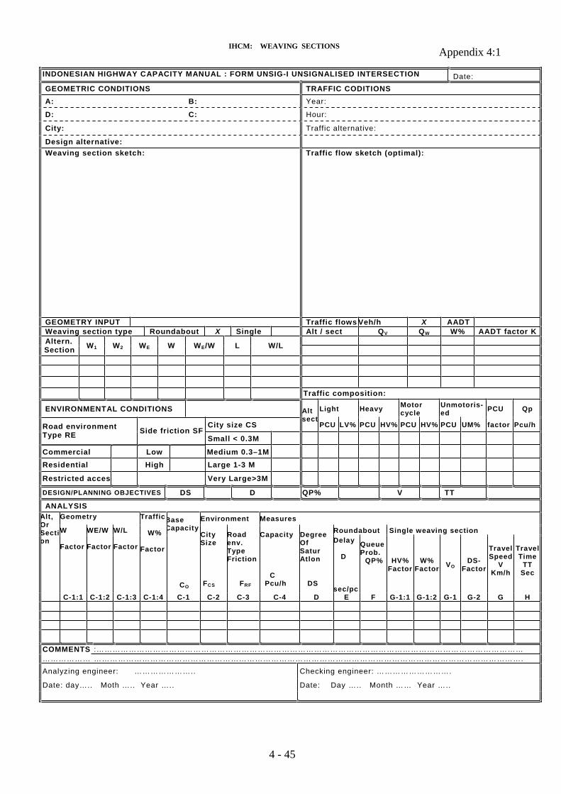
IHCM: WEAVING SECTIONS Appendix 4:1
INDONESIAN HIGHWAY CAPACITY MANUAL : FORM UNSIG-I UNSIGNALISED INTERSECTION Date:GEOMETRIC CONDITIONS TRAFFIC CODITIONSA: B: Year:
D: C: Hour:
City: Traffic alternative:
Design alternative:Weaving section sketch: Traffic flow sketch (optimal):
GEOMETRY INPUT Traffic flows Veh/h X AADTWeaving section type Roundabout X Single Alt / sect QV QW W% AADT factor KAltern.Section W1 W2 WE W WE/W L W/L
Traffic composition:
ENVIRONMENTAL CONDITIONS Light Heavy Motorcycle
Unmotoris-ed PCU Qp
City size CS
Altsect
PCU LV% PCU HV% PCU HV% PCU UM% factor Pcu/hRoad environmentType RE Side friction SF
Small < 0.3M
Commercial Low Medium 0.3–1MResidential High Large 1-3 M
Restricted acces Very Large>3M
DESIGN/PLANNING OBJECTIVES DS D QP% V TT
ANALYSISGeometry Environment Measures
Roundabout Single weaving section
Alt,OrSection
W
Factor
WE/W
Factor
W/L
Factor
Traffic
W%
Factor
BaseCapacity
CO
CitySize
FCS
Roadenv.TypeFriction
FRF
Capacity
C Pcu/h
DegreeOfSaturAtlon
DS
Delay
D
sec/pc
QueueProb. QP% HV%
FactorW%
Factor VODS-
Factor
TravelSpeed
VKm/h
TravelTime
TTSec
C-1:1 C-1:2 C-1:3 C-1:4 C-1 C-2 C-3 C-4 D E F G-1:1 G-1:2 G-1 G-2 G H
COMMENTS :…………………………………………………………………………………………………………………………………………………………… …………………………………………………………………………………………………………………………………………….Analyzing engineer: ………………….. Checking engineer: ……………………….
Date: day….. Moth ….. Year ….. Date: Day ….. Month …… Year …..
4 - 45

Chapter 5: URBAN ROADS

IHCM: URBAN ROADS
CHAPTER 5
URBAN ROADS
TABLE OF CONTENTS
1. INTRODUCTION ..............................................................................................5 – 3
1.1 SCOPE AND OBJECTIVES ................................................................................5 – 31.2 ROAD CHARACTERISTICS ...............................................................................5 – 51.3 DEFINITIONS AND TERMINOLOGY ..............................................................5 – 7
2. METHODOLOGY ..............................................................................................5 – 14
2.1 GENERAL APPROACH .....................................................................................5 – 142.2 BASIC RELATIONSHIPS ....................................................................................5 – 162.3 GEOMETRIC CHARACTERISTICS ...................................................................5 – 182.4 OVERVIEW OF THE CALCULATION PROCEDURE .....................................5 – 20
3. CALCULATION PROCEDURE FOR URBAN ROADS .............................5 – 22
3.1 OPERATIONAL ANALYSIS AND DESIGN .....................................................5 – 22STEP A: GENERAL DATA ........................................................................5 – 23
A-l: Road segments .................................................................5 – 23A-2: General input data ...........................................................5 – 23
STEP B: GEOMETRIC CONDITIONS .......................................................5 – 24B-1: Input data .........................................................................5 – 24
STEP C: TRAFFIC CONDITIONS ..............................................................5 – 26C-1: Input data .........................................................................5 – 26C-2: Traffic composition, pcu-factor and actual flow .............5 – 26C-3: Directional split class ........................................................5 – 27
STEP D: ENVIRONMENTAL CONDITIONS ...........................................5 – 28D-1: Side friction class ..............................................................5 – 28D-2: City size ............................................................................5 – 29
STEP E: ANALYSIS ....................................................................................5 – 30 E-1: Base capacity ....................................................................5 – 30
E-2: Carriageway width adjustment factor ............................5 – 30E-3: Kerb and shoulder adjustment factor .............................5 – 31E-4: Directional split or median adjustment factor ................5 – 33E-5: Side friction adjustment factor I ......................................5 – 34E-6: City size adjustment factor .............................................5 – 34E-7: Capacity ............................................................................5 – 34E-8: Degree of saturation .........................................................5 – 34E-9: Travel speed .....................................................................5 – 34E-10: Journey time .....................................................................5 – 35E-11: Results ..............................................................................5 – 35E-12: Comments ........................................................................5 – 35
5 - 1

IHCM: URBAN ROADS
STEPF: RE-ANALYSIS ............................................................................5 – 423.2 PLANNING .......................................................................................................5 – 43
4. CALCULATION PROCEDURE FOR URBAN MOTORWAYS ...............5 – 45
4.1 OPERATIONAL ANALYSIS AND DESIGN ..................................................5 – 45STEP A: GENERAL DATA ......................................................................5 – 47
A-1: Road segments ....................................................................5 – 47A-2: General input data ................................................................5 - 47
STEPB: GEOMETRIC CONDITIONS ......................................................5 – 48 B-1: Input data .............................................................................5 – 48STEP C: TRAFFIC CONDITIONS ............................................................5 – 49 C-1: Input data .............................................................................5 – 49
C-2: Traffic composition, pcu-factor and actual flow ....................5 – 49STEP D: ANALYSIS ..................................................................................5 – 50
D-1: Carriageway width and effective left shoulder width ..........adjustment factor .................................................................5 – 50
D-2: Capacity .............................................................................5 – 50D-3: Degree of saturation .............................................................5 – 51D-4: Travel speed .......................................................................5 – 51D-5: Journey time ........................................................................5 – 51D-6: Results ................................................................................5 – 51D-7: Comments ..........................................................................5 – 51
STEP E: RE-ANALYSIS .................................... .......................................5 – 524.2 PLANNING .......................................................................................................5 – 53
5. WORKED EXAMPLES .......................................................................................... 5 – 54
5.1 EXAMPLE-l: OPERATIONAL ANALYSIS OF A TWO-LANETWO-WAY ROAD ...........................................................................................5 – 54
5.2 EXAMPLE-2: OPERATIONAL ANALYSIS OF A TWO-LANE TWO-WAY ROAD ............................................................................................5 – 585.3 EXAMPLE-3: OPERATIONAL ANALYSIS OF A TWO-LANE
TWO-WAY ROAD ............................................................................................5 – 62 5.4 EXAMPLE-4: OPERATIONAL ANALYSIS OF A FOUR-LANE TWO-WAY ROAD ............................................................................................5 – 66 5.5 EXAMPLE-5: OPERATIONAL ANALYSIS OF FOUR-LANE
TWO-WAY ROAD, FOR USE IN A NETWORK ANALYSIS ......................5 – 71 5.6 EXAMPLE-6: DESIGN OF A NEW ROAD ........................................................5 – 755.7 EXAMPLE-7: PLANNING ................................................................................5 – 79 5.8 EXAMPLE-8: OPERATIONAL ANALYSIS OF URBAN MOTORWAYS ...5 – 80
6. LITERATURE REFERENCES ........................................................................5 – 83
APPENDIX 5.1: Calculation forms ......................................................................................5 – 85
5 - 2

IHCM: URBAN ROADS
1 . INTRODUCTION
1.1 SCOPE AND OBJECTIVES
1.1.1. Facility types
This manual presents procedures for the calculation of capacity and performance measures on urban and suburban roads of the following types:
Urban roads:
- Two-lane two-way roads (2/2)- Four-lane two-way roads (4/2) - without median (undivided)- with median (divided)- One-way roads (1-3/1)
Urban motorways:
Dual, two-lane carriageways with grade separated junctions.
1.1.2. Application
The road types used in this manual are defined in the Section 2.3. They are not related to theIndonesian functional road classification system (Undang-undang tentang Jalan, No. 13,1980), which was developed for a different purpose.
For each of the defined road types, the calculation procedure may be applied with confidence onlyin the following conditions:
- Flat or essentially flat terrain.- Straight or essentially straight horizontal alignment.- On segments of roads which are not affected by queuing caused by intersections, nor by
severe platooning downstream from signalised intersections.
1.1.3. Road segments
The procedures are applied to calculations for individual segments of a road. A road segment isdefined as a length of road:
- between and unaffected by signalised or major unsignalised intersections, and- having similar characteristics along its length.
Points where road characteristics change significantly automatically become the boundary of asegment even if there is no nearby intersection. The road characteristics of importance in thisrespect are set out in general in Section 1.2, and in more detail in the Sections of this manual whichdeal with each road type.
5 - 3

IHCM: URBAN ROADS
In segmenting an urban motorway, ramps and weaving areas must be separated from road segments.The procedures given in this Section relate to road segments but not to weaving areas and ramps. Asramp areas may be the critical areas for capacity, separate ramp or weaving analysis may be needed, especially in operational analysis of the road. In this case, it is recommended that theprocedures for freeway, ramps and weaving sections contained in the 1985 US HCM are used.
1.1.4. Networks
If a network or corridor is being analysed, it should be broken down into its components, as follows:
- Road segments- Signalised intersections- Unsignalised intersections- Weaving Sections
Calculations are then performed separately for each of these facility types: they are then combined to give the capacity and overall measures of performance for the system as a whole.
The procedures set out below for urban and suburban roads apply to segments without intersection effects, and consequently most of the empirical data on which this manual is based were collected on major urban and suburban through-routes and not on city streets. On city streets, where major intersections are frequent, the capacity and performance of the road systemwill depend mainly on the intersections (and weaving Sections) and not so much on the roadsegments between them. However, if a network analysis is needed, the calculation proceduresfor road segments presented below may be applied to city centre street networks in the following way:
- Calculate journey time, using the road segment procedures, as if there was no disturbance fromany intersections or weaving areas i.e. do the analysis as if no intersections or weaving areasexisted ("unobstructed journey time")
- For each major intersection or weaving area in the network, calculate delay, usingappropriate procedures from other parts of this manual
- Add the intersection/weaving delays to the unobstructed journey time, to obtain the overall journey time.
5 - 4

IHCM: URBAN ROADS
1.2 ROAD CHARACTERISTICS
The main characteristics of a road which will affect its capacity and its performance whenloaded with traffic are as follows. Any point on a particular road where there is a significant change ingeometric characteristics or in roadside activities becomes the boundary of a road segment.
1.2.1. Geometry
- Road type : roads of different type will perform differently under a given traffic load; forexample toll roads and non-toll roads.
- Width of carriageway : capacity increases with carriageway width.
- Shoulder/kerb characteristics : capacity, and speed at a given flow, increase withincreasing shoulder width. The capacity of roads with kerbs is less than those with shoulders. Capacity is reduced if there are fixed obstructions close to the edge of thecarriageway, whether the road has a kerb or a shoulder.
- Presence or absence of median (divided or undivided): well-designed medians increasecapacity.
1.2.2. Flow composition and directional split
- Directional split of traffic: capacity is highest on two-way roads when directional split is50 - 50: that is to say when the flows are equal in both directions.
- Traffic composition: if flow and capacity are measured in veh/h, traffic composition will affect capacity. However, by measuring. flow in passenger car units (pcu), as in thismanual, this effect has been accounted for.
1.2.3. Traffic control
- Controls on speeds, heavy vehicle movements, parking, etc will affect the capacity of theroad.
1.2.4. Environment
- Roadside environment and activities : the many activities in Indonesia at the roadside often conflict, sometimes severely, with flow of traffic. The effects of these conflicts, ("side friction"), is given extra attention in this manual, in comparison to that given in Western manuals.
5 - 5
IHCM: URBAN ROADS
- The following side-frictional items have been found to affect traffic significantly on Indonesian two-lane two-way roads:
- Pedestrians walking- Stopping angkot (on roadway or shoulder)- Stopping big buses (on the roadway)- Stopping unmotorised vehicles- Pedestrians crossing the road - Vehicles entering and leaving roadside premises- Parking on roadway or shoulder
Of these only pedestrian walking, stopping angkot (on the roadway), pedestrian crossing the road and exit/entry vehicles have been found to be of general significance, the rest are important only at some locations. Friction is generallydefined semi-qualitatively as either very low, low, medium, high or very high, in terms of these four generally significant items. A seventh item, parking on theroadway, is included in the carriageway width adjustment factors.
- Driver and vehicle population: the size of Indonesia and the diversity and degree of development of its urban areas mean that driver behaviour and vehicle population(the age, power and condition of vehicles, as distinct from vehicle composition)are diverse. These characteristics are incorporated into the calculation proceduresindirectly, by means of city size: smaller cities exhibit less urgent driver behaviourand a less modern vehicle fleet, leading to reduced capacities and lower speeds at a given flow, when compared with larger cities.
These characteristics are used in the calculation procedures in this manual. Most of them have also been recognized by and used in other capacity manuals. The magnitude of theireffects is however different in Indonesia.
5 - 6
IHCM: URBAN ROADS
1.3 DEFINITIONS AND TERMINOLOGY
NOTATION TERM DEFINITION
Performance measures
C Capacity(pcu/h)
Maximum stable output flow (pcu/h) at whichvehicles can be reasonably expected to traversea uniform segment of roadway during aspecified time period (15 minutes) at givengeometry, traffic flow pattern and composition,and environmental factors.
DS DEGREE OFSATURATION
Relation between actual total incoming flow(pcu/h) and capacity (pcu/h) at givengeometry, traffic flow pattern and composition,and environmental factors.
V TRAVEL SPEEDJOURNEY SPEED
Average speed of a traffic stream computed asthe length of a road segment divided by theaverage travel time of vehicles traversing thesegment (km/h).
Vo FREE FLOW SPEED (1) The theoretical speed of traffic when densityis zero, i.e, there are no vehicles present (km/h).(2) The average speed of unobstructed vehiclesover a road segment at which drivers feel comfortable traveling, under the physical, environmental, and traffic control conditions existingon an uncongested section of road segment.
TT TRAVEL TIMEJOURNEY TIME
Average time spent by vehicles traversing aroad segment of given length, including allstopped-time delay (sec/pcu).
Geometric conditions
WC CARRIAGEWAYWIDTH (m)
The width available for traffic movement.
WK KERB WIDTH (m) Distance from kerb to obstruction.
WS SHOULDER WIDTH(m)
Distance from the edge of roadway toobstruction.
WCe EFFECTIVECARRIAGEWAYWIDTH (m)
The width available for traffic movement afterreduction due to on street parking, for example.
MEDIAN Area separating traffic directions on a roadsegment.
5 - 7

IHCM: URBAN ROADS
L ROAD LENGTH Length of road segment, as if there were nodisturbance from any intersections or weavingareas.
ROAD TYPE Road type defines number of lanes and directions ona road segment: - 2-Iane 2-way (2/2) - 4-lane 2-way undivided and divided (4/2)- 1-way (1-3/1)- Motorways.
NUMBER OF LANES Number of lanes is defined from the effectivecarriageway width (Wc,) for the road segment, seeTable 1.3:1
Effective carriageway widthWCe (m)
Number oflanes
5 to 10.5 2
10.5 to 16 4
Table 1.3:1 Number of Lanes
Environmental conditions
CS CITY SIZE City size is the number of inhabitants in the city(M). Four city size classes are defined, see Table1.3:2:
City size(M in h.)
City size class CS
< 0.5 Small0.5-1.0 Medium
1.0- 3.0 Large
> 3.0 Very large
Table 1.3:2 City size classes
5 - 8

IHCM: URBAN ROADS
SF SIDEFRICTION Side friction is the impact on traffic performancefrom roadside activities on the road segment aspedestrians walking, along it or crossing, angkutankota stopping on the roadway and vehiclesentering and exiting.
Five side friction classes are used. They are decidedquantitatively:- Very low (especially if frontage road exists)- Low- Medium- High- Very high (especially if there are many
exit/entry of short-term parked vehicles).
Traffic conditions
Q ACTUAL FLOW Number of vehicles passing a point on a road perunit of time, expressed in veh/h or pcu/h.
Qv TOTAL ACTUAL FLOW (veh/h)
Total incoming flow to the road segment for both directions (veh/h).
Qp TOTAL ACTUAL FLOW (pcu/h)
Total incoming flow to the road segment for both directions (pcu/h).
SP DIRECTIONAL Flow distribution (pcu) in the two directions of aroad.
Six directional split class are used in the manu-al, i.e,100/0, 90/10,80/20,70/30,60/40 and 50/50.
P PCU-FACTOR Conversion factor to convert a vehicle flow intoan equivalent light vehicle flow.
K AADT-FACTOR Conversion factor from AADT to peak hourtraffic.
Qd DESIGN FLOW Traffic flow (pcu/h) used for planning:
Qd = AADT x K
5 - 9

IHCM: URBAN ROADS
Calculation factors
Co BASE CAPACITY(pcu /h)
Capacity of a road segment for a predetermined(ideal) set of conditions (geometry, traffic flowpattern and environmental factors).
FW CARRIAGEWAY WIDTHADJUSTMENT FACTOR
Adjustment factor for base capacity due tocarriageway width.
FKS KERB AND SHOULDERADJUSTMENT FACTOR
Adjustment factor for base capacity due to kerband/or shoulder width.
FSP DIRECTIONAL SPLIT ADJUSTMENT FACTOR
Adjustment factor for base capacity due todirectional split.
FSF SIDE FRICTION ADJUSTMENT FACTOR
Adjustment factor for base capacity due to sidefriction.
FCS CITY SIZE ADJUSTMENT FACTOR
Adjustment factor for base capacity due to citysize.
5 - 10
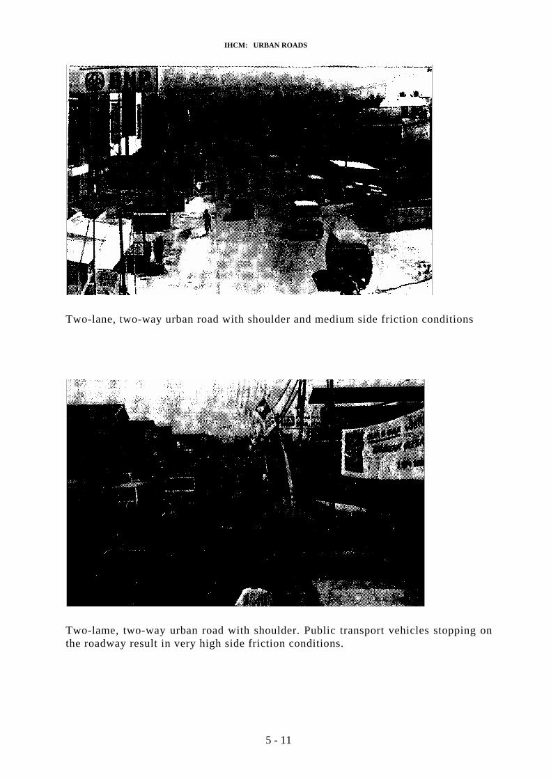
IHCM: URBAN ROADS
Two-lane, two-way urban road with shoulder and medium side friction conditions
Two-lame, two-way urban road with shoulder. Public transport vehicles stopping on the roadway result in very high side friction conditions.
5 - 11

IHCM: URBAN ROADS
Undivided, four-lane, two-way urban road with kerb and very high side friction conditions. On-street parking reduce effective carriageway width.
Two-lane, one-way urban road with shoulder and medium side friction conditions due topedestrians. The trees reduce the effective shoulder width zero m.
5 - 12

IHCM: URBAN ROADS
Undivided, four-lane, two-way urban road with kerb and very high side friction conditions. On-street parking reduce effective carriageway witdh.
Divided, four-lane, two-way urban road with kerb and low sidefriction conditions. The trees at the edge of the kerbs reduce speed and capacity.
5 - 13

IHCM: URBAN ROADS
2. METHODOLOGY
2.1 GENERAL APPROACH
2.1.1. Type of calculation
The procedures given in this manual allow the calculation of:
- the performance of a road segment under a given traffic flow and composition;- the maximum flow of traffic a road segment can carry while maintaining a
specified level of performance;- the capacity of a road segment and thus the degree of saturation (flow/capacity)
of the segment
for road segments of different types, and with particular characteristics.
2.1.2. Levels of analysis
Procedures are given in this manual to enable analysis to be carried out at one of threelevels:
- Operational analysis: The determination of the performance of an existing or proposed road segment under existing or projected traffic demand. The capacity can also be calculated, as can the maximum flow which can be carried while still maintaining a specified level of performance. This is the most detailed level of analysis.
- Design: The determination of the number of lanes needed to carry a given flow oftraffic while maintaining an acceptable performance level.
- Planning: As for design, the objective is to estimate the likely number of lanesneeded for a projected road, but the information on flow is likely to be given only as estimated AADT and the details of geometry and other inputs can only be assumed.
The methods used in operation design and planning analyses are related and differ mainlyin the level of detail in the inputs, and outputs. In most cases, the steps in analysis for operational and design analyses will be virtually identical. Steps in planning analysis are very much simpler in most cases.
The calculation procedures given in this manual are in most cases similar, at least in general form, to those in the 1985 U.S. Highway Capacity Manual (US HCM). This is intentional,as users of this manual may already be familiar with the US HCM procedures. Indetail however, the procedures are not the same: the complex effect of grades are of lessimportance in urban than in rural areas in determining speeds. This manual also uses somedifferent variables. Where variables are in common, their values for Indonesian conditions are often quite different from those from the US HCM.
5 - 14

IHCM: URBAN ROADS
2.1.3. Capacity
Capacity is defined as the maximum flow past a point on the road that can be sustained on anhourly basis under prevailing conditions. This is a two-way flow for two-lane and four-lane two-way roads, and a one-way flow for urban motorways and one-way streets.
2.1.4. Measures of road performance
This manual uses journey speed (synonymous with travel speed) as the main measure of performance of road segments as it is easy to understand and to measure. Journey speed is defined in this manual as the space mean speed of motor vehicles over the road segment:
V = L / TT x 3600
where V = space mean speed (km/h)L = length of segment (km)TT = mean travel time of motor vehicles over the segment (secs)
The procedures outlined below also allow the degree of saturation (flow/capacity) to be determined. This is a widely used measure to indicate whether a road segment is expected to have capacity problems or not.
Thus on the one hand, speed is a simple measure to which drivers can relate, which can also beused in economic analysis. On the other hand, flow/capacity is a quick indicator ofwhether capacity problems are likely to exist.
2.1.5. Level of service
In the US HCM road performance is represented by Level of Service (LOS): a qualitative measure reflecting the drivers' perception of the quality of driving. LOS is related in turn to aquantitative proxy measure, such as density, per cent passing opportunities or journey speed.The level of service concept was developed for use in the United States and the LOS definitionsdo not directly apply to Indonesia. It is also difficult to produce alternative definitions forIndonesia whose meanings would be clear. For this reason, speed and degree of saturation areused in this manual. Speeds, however, are much lower in Indonesia than in the USA at agiven degree of saturation (flow/capacity = Q/C).
2.1.6. Traffic flow and composition
Throughout the manual the traffic flow values reflect traffic composition, by expressing flow in passenger car units (pcu).
See Chapter 1 Section 4 for definitions regarding which vehicle types that. are included aslight vehicles, heavy vehicles, motorcycles and unmotorised vehicles.
5 - 15
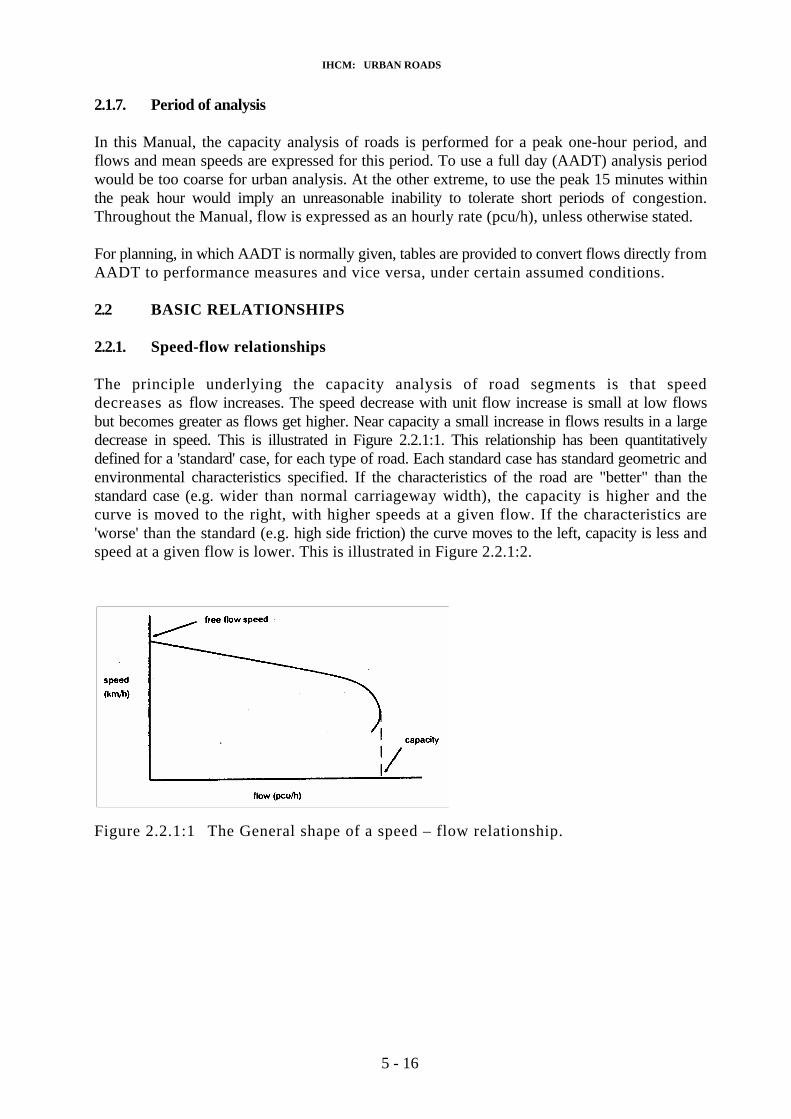
IHCM: URBAN ROADS
2.1.7. Period of analysis
In this Manual, the capacity analysis of roads is performed for a peak one-hour period, and flows and mean speeds are expressed for this period. To use a full day (AADT) analysis period would be too coarse for urban analysis. At the other extreme, to use the peak 15 minutes withinthe peak hour would imply an unreasonable inability to tolerate short periods of congestion.Throughout the Manual, flow is expressed as an hourly rate (pcu/h), unless otherwise stated.
For planning, in which AADT is normally given, tables are provided to convert flows directly fromAADT to performance measures and vice versa, under certain assumed conditions.
2.2 BASIC RELATIONSHIPS
2.2.1. Speed-flow relationships
The principle underlying the capacity analysis of road segments is that speed decreases as flow increases. The speed decrease with unit flow increase is small at low flowsbut becomes greater as flows get higher. Near capacity a small increase in flows results in a large decrease in speed. This is illustrated in Figure 2.2.1:1. This relationship has been quantitatively defined for a 'standard' case, for each type of road. Each standard case has standard geometric andenvironmental characteristics specified. If the characteristics of the road are "better" than the standard case (e.g. wider than normal carriageway width), the capacity is higher and thecurve is moved to the right, with higher speeds at a given flow. If the characteristics are 'worse' than the standard (e.g. high side friction) the curve moves to the left, capacity is less andspeed at a given flow is lower. This is illustrated in Figure 2.2.1:2.
Figure 2.2.1:1 The General shape of a speed – flow relationship.
5 - 16
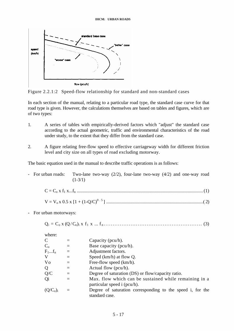
IHCM: URBAN ROADS
Figure 2.2.1:2 Speed-flow relationship for standard and non-standard cases
In each section of the manual, relating to a particular road type, the standard case curve for thatroad type is given. However, the calculations themselves are based on tables and figures, which areof two types:
1. A series of tables with empirically-derived factors which "adjust" the standard caseaccording to the actual geometric, traffic and environmental characteristics of the road under study, to the extent that they differ from the standard case.
2. A figure relating free-flow speed to effective carriageway width for different frictionlevel and city size on all types of road excluding motorway.
The basic equation used in the manual to describe traffic operations is as follows:
- For urban roads: Two-lane two-way (2/2), four-lane two-way (4/2) and one-way road (1-3/1)
C = Co x f1 x...fn ........................................................................................................... (1)
V = Vo x 0.5 x [1 + (1-Q/C)0 . 5 ] .................................................................................. ( 2)
- For urban motorways:
Qi = Co x (Q / Co)i x f1 x ... f n . . . . . . . . . . . . . . . . . . . . . . . . . . . . . . . . . . . . . . . . . . . . . . . . . . . . . . . (3)
where:C = Capacity (pcu/h).Co = Base capacity (pcu/h). F1...fn = Adjustment factors.V = Speed (km/h) at flow Q.Vo = Free-flow speed (km/h).Q = Actual flow (pcu/h).Q/C = Degree of saturation (DS) or flow/capacity ratio. Qi = Max. flow which can be sustained while remaining in a
particular speed i (pcu/h).(Q/Co)i = Degree of saturation corresponding to the speed i, for the
standard case.
5 - 17

IHCM: URBAN ROADS
2.2.2. Capacity
Referring to Equation (1), (2) and (3), when the road is operating at capacity, (Q/C) = 1.00 bydefinition. If the actual conditions are the same as the standard case, then all the adjustmentfactors f1 . . fn become 1.0 and the capacity becomes equal to the standard capacity, Co. But if any characteristics of the road are non-standard, then one or more of the factors f1...fnbecome 1.0 and the resulting "capacity" will be either lower than Co if the product of allthe factors < 1.0 (sub-standard road) or higher than Co if the product of all the factors > 1.0(over-standard road).
2.2.3. Degree of saturation and speed
The degree of saturation (flow/capacity) is used in the manual in two different ways for two different purposes:
1. Speeds are related to flow/capacity ratios.
2. Flow/capacity ratios can be calculated to indicate quickly segments which have capacity problems. The effects of different ways of solving capacity problems can also be estimated. Suppose, for example, a road had a forecast flow of 2600 pcu/h and a calculated capacity of 2900 pcu/h, giving an unacceptably high degree of saturation of0.9. Alternative solutions could be explored through Equation (1) to (3), forexample reducing friction or widening the road, by selecting adjustment factors fordesired friction or desired width.
2.3 GEOMETRIC CHARACTERISTICS
2.3.1. Two-lane two-way roads
This road type encompasses all two-way roads with a carriageway width of up to and including10.5 metres. For wider two-way roads the procedures in Section 2.3.2 (four-lane two-wayroads) should be followed. (Note: for roads of 9.5 m to 11.5 m in width, the procedures inthis Section and those in Section 2.3.2 should give approximately the same resu Its).
The standard road of this type is defined as follows:
- Seven metre carriageway width - Shoulders of effective width of at least 2 m on each side- No median- Directional traffic split of 50 - 50- Low side friction- City size 1.0 - 3.0 M- Essentially level terrain - Essentially straight alignment
5 - 18

IHCM: URBAN ROADS
2.3.2. Four-lane two-way roads
This road type encompasses all two-way roads with a carriageway width greater than 10.5metres and up to 16.0 metres.
The standard road of this type is defined as follows:
- Fourteen metre carriageway width - Kerbed: with at least 2 m clearance to roadside obstructions- No median- Directional traffic split of 50 - 50- Low side friction- City size 1.0 - 3.0 M- Essentially level terrain - Essentially straight alignment
2.3.3. One-way roads
This road type encompasses all one-way roads with .a carriageway width from 5.0 m up to andincluding 10.5 metres.
The standard road of this type is defined as follows:
- Seven metre carriageway width- Kerbed: with at least 2 m clearance to roadside obstructions- No median- Low side friction- City size 1.0 - 3.0 M- Essentially level terrain - Essentially straight alignment
2.3.4. Urban motorways
This road type encompasses all urban 4-lane (2 carriageways, each of two lanes) fully grade-separated roads. The standard road of this type is:
- Four lanes, each of 3.6 m width (two 7.2 metre carriageways).- Effective left shoulder width of 2.0 m.- City size > 3.0 M. - Zero side friction (completely restricted access).- Complete grade separation.- No motorcycles or unmotorised vehicles in the traffic.- Essentially level terrain. - Essentially straight alignment.
To date, all roads in Indonesia of this type are operated as toll roads.
5 - 19

IHCM: URBAN ROADS
2.4 OVERVIEW OF THE CALCULATION PROCEDURE
A flow chart of the calculation procedure is illustrated in Figure 2.4:1 for urban roads andFigure 2.4:2 for urban motorways. The different steps are described in detail in Section 3 and4.
Figure 2.4:1 Flow chart for analysis of urban roads
5 - 20

IHCM: URBAN ROADS
Figure 2.4:2 Flow chart for analysis of urban motorways
The following forms are used for the calculations:
a) Urban Roads
ROAD-1 GENERAL, GEOMETRYROAD-2 TRAFFIC, ENVIRONMENTROAD-3 ANALYSIS, RESULTS, COMMENTS
b) Urban Motorways
ROAD-4 GENERAL, GEOMETRY, TRAFFICROAD-5 ANALYSIS, RESULTS, COMMENTS
The forms are presented in Appendix 5:1.
5 - 21

IHCM: URBAN ROADS
3 . CALCULATION PROCEDURE FOR URBAN ROADS
3.1 OPERATIONAL ANALYSIS AND DESIGN
The objectives of operational analysis for a particularly road segment, under an existing or projected set of geometric, traffic and environmental conditions can be:
- to determine capacity;- to determine the Q/C ratio associated with a projected traffic flow;- to determine the speed in which the road will operate.
The main objective of design is to determine the number of standard lanes needed, but can also be to estimate the effect of a change in design, such as whether to construct a shoulder or a kerb. The calculation procedures followed for operational analysis and fordesign are the same.
The general approach is to compute the capacity and speed on the urban roads. These are calculated by using following equation:
C = Co x FW x FKS x FSD x FSF x FCS
V = VOx 0.5 x [1 + (1 - Q /C)0.5]
where:C = Capacity (pcu / h) Co = Base capacity (pcu / h) FW = Carriageway width adjustment factorFKS = Kerb and shoulder adjustment factorFSD = Directional split adjustment factor (FSP. is not valid for one-
way roads) FSF = Side friction adjustment factorFCS = City size adjustment factorV = Speed (km/h) at flow Q VO = Free-flow speed (km/h)Q = Actual flow (pcu/h) Q/C = Degree of saturation (DS)
The following steps carried out in operational analysis or design, using the Forms ROAD-1, ROAD-2 and ROAD-3, are given in Appendix 5:1.
5 - 22

IHCM: URBAN ROADS
STEP A : GENERAL DATA TEP A-1 : ROAD SEGMENTSS
- Divide the road into segments. A road segment is defined as a length of road:
- between and unaffected by signalised or major unsignalised intersections, and- having similar characteristics along its length.
Points where road characteristic change significantly automatically become theboundary of a segment even if there is no nearby intersection. If severalgeometric alternatives are being explored, each may be entered into a separate formand be identified by case number.
- Fill in road segment identification (site name/section/city) and segment length (L) inseparate forms for each segment, in Section GENERAL (Form ROAD-1). Follow theremaining steps for each segment and case.
STEP A-2 : GENERAL INPUT DATA
Fill in date and personnel in Section GENERAL (Form ROAD-1)
5 - 23

IHCM: URBAN ROADS
STEP B : GEOMETRIC CONDITIONS Insert the geometric data in the spaces provided in Section GEOMETRY (Form ROAD-1). The geometric terms used are shown in Figure B:1 below.
Figure B:1 Illustration of the geometric terms used.
STEP B-1 : INPUT DATA
Enter the following input data in Section GEOMETRY (Form ROAD-l):
- Whether the segment has a shoulder or a kerb, or both.
- Shoulder level: difference between levels of shoulder and carriageway.
- Whether the segment has a median or not for four-lane two-way roads (4/2)
- Effective carriageway width (m) (total both carriageways, even if divided by a median for four-lane two-way roads).
- Effective shoulder width or distance from kerb to obstruction on both sides.
- If the road has a median, determine median width (m) and median continuity (nogaps/few gaps/frequent gaps)
- Few gaps: gap exists, but fewer than an average of one per 500 m Frequent gaps: an average of one or more gaps per 500 m
- If the road has only shoulders on both sides, calculate average effective shoulderwidth (m).
5 - 24

IHCM: URBAN ROADS
- If the road has only kerbs on both sides, calculate average distance to roadsideobstructions (m).
- Source of geometric data.
5 - 25

IHCM: URBAN ROADS
STEP C : TRAFFIC CONDITIONS Insert the traffic data in the boxes provided in Section TRAFFIC (Form ROAD-2) and determine traffic composition, pcu-factor and actual flow in pcu/h.
STEP C-1 : INPUT DATA
Enter the following input data in Section TRAFFIC (Form ROAD-2):
- pcu values
For simplicity, constant pcu values are used as follow:
Light vehicle (LV) 1.00Heavy vehicle (H V) 1.20Motorcycle (MC) 0.25Unmotorised vehicle (UM) 0.80
- Period (Column 1)
- Total peak hour flow in both directions (existing or forecast) by vehicle type(Column 2 to 5)
- Year of traffic data
- Source of traffic data
STEP C-2:TRAFFIC COMPOSITION,PCU-FACTOR AND ACTUAL FLOW
- Calculate the actual flow (veh/h) and enter the results into Column 6 (Form ROAD2),using following equation:
QV = QLV + QHV + QMC + QUM
- Calculate traffic composition for each vehicle type and enter the results into Column 7to 10 (Form ROAD-2).
- Calculate pcu-factor and enter the results into Column 11 (Form ROAD-2), using following equation:
P = (LV% x pcuLV + HV% x pcuHV + MC% x pcuMc + UM% x pcuUM)/100
- Determine the actual flow (pcu/h) and enter the results into Column 12 (FormROAD-2), using following equation:
QP = QV x P
5 - 26

IHCM: URBAN ROADS
STEP C-3 : DIRECTIONAL SPLIT CLASS
- Enter directional split class into Column 13 (Form ROAD-2).
Other traffic information (eg. AADT) are used for planning purposes and need not be filledin for operational analysis or design. If necessary, convert classified flow into pcu.
5 - 27

IHCM: URBAN ROADS
STEP D : ENVIRONMENTAL CONDITIONS Enter the appropriate environmental data in Section ENVIRONMENT (Form ROAD-2), bydeleting inappropriate values.
STEP D-1 : SIDE FRICTION CLASS
Side friction class is determined by classifying each of the 3 components listed below into oneof the 5classes as shown in Table D-1:1. This can be done by an engineer with a knowledge of the road or ofthe area.
Side friction class Side friction item Very
lowLow
(few)Medium(some)
High(many)
Veryhigh
Pedestrian movements 0 1 2 4 7
Angkutan kota stopping on the roadway 0 1 3 6 9
Vehicles turning into or out of the segment 0 1 3 5 8
Notes: - Pedestrian movements including pedestrian walking and pedestrian crossing - Very low: especially if frontage road exists (restricted access) - Very high: especially if there are many exit/entry of short-term parked vehicles
Table D-1:1 Side friction code
The numbers are then added to get a total score and the side friction class is determined as indicated in Table D-1:2
Total score Side friction class
0 - 1 Very low
2 - 5 Low
6 - 11 Medium
12 - 18 High
19 - 24 Very high
Table D-1:2 Side friction class based on total score
If there is insufficient information or if looking a long period ahead, medium friction should be assumed.
5 - 28

IHCM: URBAN ROADS
The actual values for each component of friction, corresponding to the very low, low, medium,high and very high categories, are shown in Table D-1:3 :
Side friction quantity No Friction item Very
lowLow Medium High Very
high
1. Pedestrian walking (ped/h) 0 0- 80 80 -120 120-220 > 2202. Pedestrian crossing (ped/h/km) 0 0-200 200-500 500-1300 >13003. Stopping angkot on the roadway
(veh / h / km)0 0-100 100-300 300- 700 > 700
4. Exit/entry vehicles (veh/h/km) 0 0-200 200-500 500-800 >800
Table D-1:3 Side friction quantity
The values shown in this table could be used as a basis for determination of side frictionlevel as indicated in Table D-1:1.
STEP D-2: CITY SIZE
Enter city size (M inh) at the bottom in Form ROAD-2.
5 - 29

IHCM: URBAN ROADS
STEP E : ANALYSISSelect values of each of the factors from the tables indicated in Section ANALYSIS (Form ROAD-3). The values should be appropriate to the geometric, traffic and environmentalconditions described in Form ROAD-1 and ROAD-2.
STEP E-1 : BASE CAPACITY
Determine the base capacity (C0) from Table E-1:1 and enter the value into Column 2(Form ROAD-3).
Type of urban roads 2/2 4/2 1-3/1
Co (pcu/h) 2900 5700 3200
Table E.1:1 Base capacity (Co) for urban roads.
STEP E-2 : CARRIAGEWAY WIDTH ADJUSTMENT FACTOR
Determine the carriageway width factor (FW) from Table E-2:1 and enter the value into Column 3 (Form ROAD-3).
Effectivecarriagewaywidth WCe (m)
5 6 7 8 9 10 11 12 13 14 15 16
2/2 0.66 0.83 1.00 1.07 1.14 1.21 1.43
4/2 0.58 0.68 0.79 0.90 1.00 1.03 1.05FW
1-3/1 0.66 0.83 1.00 1.05 1.10 1.15 1.36
Notes : Use linear interpolation for intermediate values. Effective carriageway width is thewidth available for traffic movement. On-street parking for example, reduces effective width 3.0 m.
Table E-2:1 Carriageway width adjustment factors (FW)
5 - 30

IHCM: URBAN ROADS
STEP E-3 : KERB AND SHOULDER ADJUSTMENT FACTOR
a) Roads with shoulders
Determine the shoulder factor from Table E-3:1 which assumes shoulders are level with thecarriageway and of firm material, and enter the value into Column 4 (Form ROAD-3). Ifshoulder level is 10 cm or more different from that of the carriageway it is suggested thatthe FKS for zero effective width shoulder should be used.
Effective shoulder width WSe (m) 0 0.5 1.0 1.5 >2.0
2/2 0.85 0.89 0.93 0.96 1.00
4/2 0.96 0.99 0.01 1.04 1.06FKS
1-3/1 0.94 0.98 1.02 1.06 1.10
Notes : (1) The table assumes two shoulders of equal effective width; if shoulders oneach side have different effective widths, take the average effective width.
(2) Effective width is the width of the available shoulder. For example, a line of trees down the middle of the shoulder would halve the effective width.
Table E-3:1 Effective shoulder width adjustment (FKS) factors(l)
b) Roads with kerbs
Determine the kerb factor from Table E-3:2 and enter the value into Column 4 (Form ROAD-3). The adjustment factor varies according to the distance of obstructions (solid objects)from the line of the kerb (edge of the carriageway).
Distance from kerb to obstruction WKe (m) 0 0.5 1.0 1.5 >2.0
2/2 0.85 0.86 0.88 0.89 0.90
4/2 0.96 0.97 0.98 0.99 1.00FKS
1-3/1 0.94 0.96 0.97 0.99 1.00
Table E-3:2 Kerb distance to obstruction adjustment (FKS) factors
Kerbs have two effects :
- They reduce speed and capacity, even when there is no friction;
- When there is friction, the kerb tends to confine some of it to the carriageway which could otherwise take place on the shoulder.
The kerb adjustment factors in Table E-3:2 include only the former effect. The latter is included in the side friction adjustment factor.
5 - 31

IHCM: URBAN ROADS
c) Roads with shoulder and kerb
If the road has a shoulder on one side and a kerb on the other, take the appropriate shoulder factor from Table E-3:1 and the appropriate kerb factor from Table E-3:2, and make the factor(FKS) equal to the average of there two values. The value is then entered into Column 4 (FormROAD-3).
5 - 32

IHCM: URBAN ROADS
STEP E-4 : DIRECTIONAL SPLIT OR MEDIAN ADJUSTMENT FACTOR
Determine the directional split or median factor (FSP) from Table E-4:1 or E-4:2 below and enter the value into Column 5 (Form ROAD-3).
Table E-4:1 gives the directional split adjustment factors for two-lane two-way (2/2) and four-lane two-way (4/2) undivided roads.
Directional split SP 50-50 60-40 70-30 80-20 90-10 100-0
2/2 1.00 0.94 0.88 0.82 0.76 0.70FSP 4/2 undivided 1.00 0.97 0.94 0.91 0.89 0.85
Table E-4:1 Directional split adjustment factors (FSP)
For four-lane two-way roads (4/2) with medians (divided), the presence of a median renders thedirectional split factor inapplicable. A median also removes the possibility of interactionbetween opposing streams and so increases capacity and performance. Table E-4:2 gives themedian adjustment factors (FSP):
Median continuity FSP
No gaps 1.12
Few gaps(l) 1.05
Frequent gaps(') 0.98
Notes : (1) Gaps exist, but fewer than an average of one per 500 m(2) An average of one or more gaps per 500 m
Table E-4:2 Median adjustment factors (FSP):
The greatest benefits to capacity occur if the median is continuous. (This does not necessarily meanthat a continuous median is always preferable to a broken one). A 'gap' is defined as a breakbig enough for a four-wheeled vehicle and where turning movements or U-turns are permitted. InIndonesia, narrow medians are the norm on non-grade-separated facilities. Consequently, turnsand U-turns through gaps in the median disrupt traffic flow and partly negate the beneficial capacityeffects of a median. Where gaps are frequent and the median narrow, capacities may be similarto or even below, an otherwise similar undivided road. Medians which are wide enough to contain turning pockets are rare in Indonesia.
5 - 33
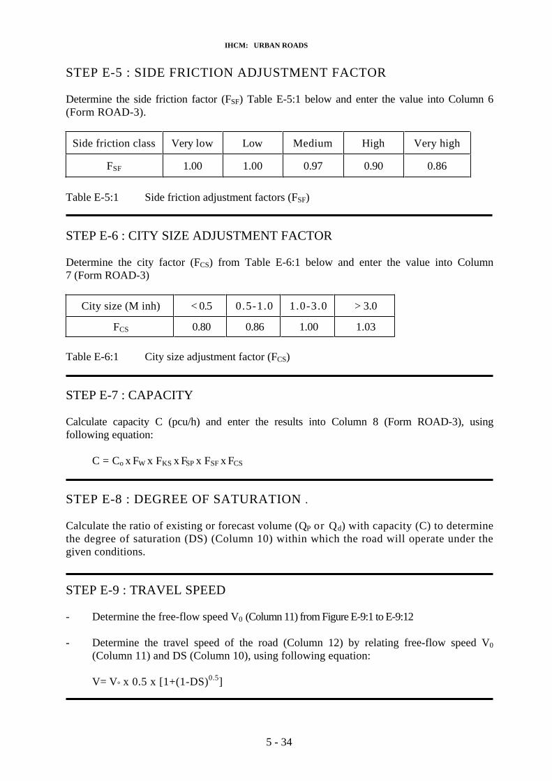
IHCM: URBAN ROADS
STEP E-5 : SIDE FRICTION ADJUSTMENT FACTOR
Determine the side friction factor (FSF) Table E-5:1 below and enter the value into Column 6 (Form ROAD-3).
Side friction class Very low Low Medium High Very high
FSF 1.00 1.00 0.97 0.90 0.86
Table E-5:1 Side friction adjustment factors (FSF)
STEP E-6 : CITY SIZE ADJUSTMENT FACTOR
Determine the city factor (FCS) from Table E-6:1 below and enter the value into Column7 (Form ROAD-3)
City size (M inh) < 0.5 0.5-1.0 1.0-3.0 > 3.0
FCS 0.80 0.86 1.00 1.03
Table E-6:1 City size adjustment factor (FCS)
STEP E-7 : CAPACITY
Calculate capacity C (pcu/h) and enter the results into Column 8 (Form ROAD-3), usingfollowing equation:
C = Co x FW x FKS x FSP x FSF x FCS
STEP E-8 : DEGREE OF SATURATION .
Calculate the ratio of existing or forecast volume (QP or Qd) with capacity (C) to determinethe degree of saturation (DS) (Column 10) within which the road will operate under thegiven conditions.
STEP E-9 : TRAVEL SPEED
- Determine the free-flow speed V0 (Column 11) from Figure E-9:1 to E-9:12
- Determine the travel speed of the road (Column 12) by relating free-flow speed V0(Column 11) and DS (Column 10), using following equation:
V= V° x 0.5 x [1+(1-DS)0.5]
5 - 34

IHCM: URBAN ROADS
STEP E-10 : JOURNEY TIME
- Calculate the average journey time (Column 13) in sec/km if a network analysis is being undertaken, or if the results of several segments of road. are to be combined, using following equation:
Average journey time = 3600/V
- Calculate the section journey time TT (Column 14) in sec, using following equation:
TT = L x Average journey time
STEP E-11 : RESULTS
Enter the results from the previous step into Section RESULTS of the worksheet (FormROAD-3).
STEP E-12 : COMMENTS
Enter any comments into Section COMMENTS of the worksheet (Form ROAD-3).
5 - 35

IHCM: URBAN ROADS
Figure E-9:1 Free-flow speed (Vo) - effective carriageway width (WCe) model for differentfriction level (SF) and city size (CS) > 3.0 M on 2-lane 2-way roads (2/2)
Figure E-9:2 Free-flow speed (Vo) - effective carriageway width (WCe) model for different friction level (SF) and city size (CS) 1.0 - 3.0 M on 2-lane 2-way roads (2/2)
5 - 36

IHCM: URBAN ROADS
Figure E-9:3 Free-flow speed (Vo) - effective carriageway width (WCe) model for differentfriction level (SF) and city size (CS) 0.5 - 1.0 M on 2-lane 2-way roads(2/2)
Figure E-9:4 Free-flow speed (Vo) - effective carriageway width (WCe) model fordifferent friction level (SF) and city size (CS) < 0.5 M on 2-lane 2-way roads (2/2).
5 - 37

IHCM: URBAN ROADS
Figure E-9:5 Free-flow speed (Vo) - effective carriageway width (WCe) model for different friction level (SF) and city size (CS) > 3.0 M bn 4-lane 2-way roads(4/2).
Figure E-9:6 Free-flow speed (Vo) - effective carriageway width (WCe) model for different friction level (SF) and city size (CS) 1.0 - 3.0 M on 4-lane 2-wayroads (4/2).
5 - 38

IHCM: URBAN ROADS
Figure E-9:7 Free-flow speed (V0) - effective carriageway width (Wce) model for different friction level (SF) and city size (CS) 0.5 - 1.0 M on 4-lane 2-way roads (4/2)
Figure E-9:8 Free-flow speed (Vo) - effective carriageway width (WCe) model fordifferent friction level (SF) and city size (CS) < 0.5 M on 4-lane 2-way roads (4/2)
5 - 39

IHCM: URBAN ROADS
Figure E-9:9 Free-flow speed (Vo) - effective carriageway width (WCe) model for differentfriction level (SF) and city size (CS) > 3.0 M on 1-way roads (1-3/1)
Figure E-9:10 Free-flow speed (Vo) - effective carriageway width (WCe) model fordifferent friction level (SF) and city size (CS) 1.0 - 3.0 M on 1-way roads(1-3/1)
5 - 40

IHCM: URBAN ROADS
Figure E-9:11 Free-flow speed (Vo) - effective carriageway width (WCe) model fordifferent friction level (SF) and city size (CS) 0.5 - 1.0 M on 1-way roads(1-3/1)
Figure E-9:12 Free-flow speed (Vo) - effective carriageway width (WCe) model for differentfriction level (SF) and city size (CS) < 0.5 M on 1-way roads (1-3/1)
5 - 41

IHCM: URBAN ROADS
STEP F : RE-ANALYSISIf the performance of the road segment is found to be inadequate, in terms of expected speed orexpected Q/C ratio, then improvements to the road geometry, or measures to reduce friction,should be considered. The effects of these changes may be assessed by repeating the analysis, usingthe new values of geometry, etc, on a fresh worksheet. This would be given a new case number.
5 - 42

IHCM: URBAN ROADS
3.2 PLANNING
For planning, the design of the road and the traffic and environmental data would be known ingeneral, but not in detail, and forecast traffic flow would be given in AADT, rather than aspeak hour flow. Consequently, certain assumptions about geometric design, traffic andenvironment have to be made. The relationship between the flow in the peak hour or design flow (Qd)and AADT must also be assumed. This relationship is normally expressed as'AADT-factor', as follows : Q = AADT x K
3.2.1. Two-lane two-way roads
The assumptions used for planning two-lane two-way roads are as follows:
Geometry: 7 m carriageway, 2 m effective shoulder width Traffic: 60- 40 directional splitEnvironment: Medium friction
City size 1.0 - 3.0 MAADT-factor(K): 0.095
On the basis of these assumptions, the procedures used in operation and design have been applied toproduce Table 3.2.1:1 which relates AADT to road performance as measured by peak hourspeeds and Q/C ratios.
Speed (km/h) 39 35 31 27 21
Q / C 0.24 0.54 0.76 0.91 1.00
AADT (pcu) 6,800 15,000 21,200 25,400 27,800
Table 3.2.1:1 Maximum AADT vs speed and Q/C ratio for planning two-lane two-way roads (2/2)
3.2.2. Four-lane two-way roads
The assumptions used for planning four-lane two-way roads are as follows:
Geometry: Kerbed 14 m carriageway, no median, at least 2 m from kerb to roadsideobstructions.
Traffic: 60- 40 directional split
Environment: Medium frictionCity size 1.0 - 3.0 M
AADT-factor(K): 0.095
5 - 43

IHCM: URBAN ROADS
On the basis of these assumptions, the procedures used in operation and design have beenapplied to produce Table 3.2.2:1 which relates AADT to road performance as measured by peakhour speeds and Q/C ratios.
Speed (km/h) 53 48 42 37 28
Q / C 0.26 0.53 0.77 0.91 1.00
AADT (pcu) 14,500 29,800 43,700 51,400 56,500
Table 3.2.2:1 Maximum AADT vs speed and Q/C ratio for planning four-lane two-way roads (4/2)
3.2.3 One-way roads
The assumptions used for planning one-way roads are as follows:
Geometry: Kerbed 7 m carriageway, at least 2 m from kerb to roadside obstructions. Environment: Medium friction
City size 1.0 - 3.0 MA ADT-factor(K): 0.095
On the basis of these assumptions, the procedures used in operation and design have been applied toproduce Table 3.2.3:1 which relates AADT to road performance as measured by peakhour speeds and Q/C ratios.
Speed (km/h) 53 48 42 37 28
Q / C 0.26 0.53 0.77 0.91 1.00
AADT (pcu) 8,400 17,300 25,300 29,700 32,700
Table 3.2.3:1 Maximum AADT vs speed and Q/C ratio for planning one-way roads (1-3/1)
Thus, estimates of AADT may be made directly from a selected speed or Q/C ratio using Table 3.2.1:1, 3.2.2:1 or 3.2.3:1. Alternatively, with a given AADT, the speed and Q/C ratio at which the planned road will operate, can immediately be estimated.
The performance of a planned road, in terms of speed or Q/C ratio, resulting from a given AADT may be obtained directly from Table 3.2.1:1, 3.2.2:1 or 3.2.3:1. This table can also be usedto estimate the AADT which could be carried while maintaining speed or Q/C ratio within given limits. No worksheet is needed. However, if conditions are known to be very differentfrom the assumed conditions given in Section 3.2.1, 3.2.2 or 3.2.3 then appropriate value(s)should be used and an operational/design analysis performed instead. This would first requireeconversion of AADT to peak hour, using AADT-factor (default: K = 0.095). Examples of caseswhere an operational analysis would be needed are:
- if the K is expected to be quite different from 0.095; put the new K value into Section TRAFFIC of the worksheet (Form ROAD-2)
- if it is known that the facility will have a kerb rather than a shoulder.
5 - 44

IHCM: URBAN ROADS
4. CALCULATION PROCEDURE FOR URBAN MOTORWAYS
The Indonesian empirical data used in this Section are based on one urban freeway, so the adjustmentfactors are based on those in the US HCM (TRB, 1985). The small amount of data on which thisSection is based means that less confidence can be placed on results of calculations for this type ofroad than for those in Section 3.
For urban motorways, all operational and design analysis is done separately by direction. For planning, both directions are combined. As in Sections 3, analysis is by total carriagewaywidth and not by the number of lanes. This is because, in Indonesia, as capacity is approached thetwo-lane carriageway begins to operate as a three-lane carriageway, with moving trafficutilizing the shoulder. This behavioural characteristic also makes it difficult to extrapolatefrom the dual-two lane to the dual-three lane case.
4.1 OPERATIONAL ANALYSIS AND DESIGN
The objectives of operational analysis for a particularly road segment, under an existing or projected set of geometric, traffic and environmental conditions can be:
- to determine capacity- to determine the Q/C ratio associated with a projected traffic flow- to determine the speed in which the motorway will operate
The main objective of design is to determine. the number of standard lanes needed, but can also be to estimate the effect of a change in design. The calculation procedures followed foroperational analysis and for design are the same.
The general approach is to compute the flow rates, by direction, for each speed and compare thesewith the existing or projected flow rate for each direction on the motorway. The flow rates inone direction for each speed values are calculated using following equation:
Qi = 4600 x (Q / Co)i x FW
where:Qi = Maximum one-way flow that can be sustained while speeds remain in
speed i (pcu/h)(Q/Qo)i = Ratio of flow to ideal capacity for speed i (C0 = 4600 pcu/h)FW = Factor for narrow lanes and effective shoulder width
5 - 45

IHCM: URBAN ROADS
The Q / C0 equivalent to the various speed values are shown in Table 4.1:1
Speed Vi (km/h) (Q/Co)i
7570655845
0.400.610.750.891.00
Table 4.1:1 Speed and (Q/Co) equivalencies
The following steps are followed in operational analysis or design, using the Form ROAD-4 andROAD-5.
5 - 46

IHCM: URBAN ROADS
STEP A : GENERAL DATA STEP A-1 : ROAD SEGMENTS
- Divide the road into segments. A road segment is defined as a length of road:
- between and unaffected by signalised or major unsignalised intersections, and- having similar characteristics along its length.
Points where road characteristics change significantly automatically become the boundary of a segment even if there is no nearby intersection. If several geometric alternatives are being explored, each may be entered into a separate form and be identified by case number.
In segmenting an urban motorway, ramps and weaving areas must be separated from roadsegments. The procedures given in this Section relate to road segments but not to weavingareas and ramps. As ramp areas may be the critical areas for capacity, separate ramp orweaving analysis may be needed, especially in operational analysis of the road. In thiscase, it is recommended that the procedures for freeway, ramps and weaving Sections contained in the 1985 US HCM are used.
- Fill in road segment identification (site name/section/city) and segment length (L) in separate forms for each segment, in Section GENERAL (Form ROAD-4). Follow theremaining steps for each segment and case.
STEP A-2 : GENERAL INPUT DATA
Fill in date personnel in section GENERAL (Form ROAD-4)
5 - 47

IHCM: URBAN ROADS
STEP B : GEOMETRIC CONDITIONS Insert the geometric data in the spaces provided in Section GEOMETRY (Form ROAD-4).
STEP B-1 : INPUT DATA
Enter the following input data in Section GEOMETRY (Form ROAD-4):
- Effective carriageway width (m) of both carriageways
- Effective shoulder width (m) of both left shoulders
- Median width (m)
- Source of geometric data
5 - 48

IHCM: URBAN ROADS
STEP C : TRAFFIC CONDITIONSInsert the traffic data in the boxes provided in Section TRAFFIC (Form ROAD-4) anddetermine traffic composition, pcu-factor and actual flow in pcu/h.
STEP C-1 : INPUT DATA
Enter the following input data in Section TRAFFIC (Form ROAD-4):
- pcu values
For simplicity, constant pcu values are used as follow:
Light vehicle (LV) 1.00Heavy vehicle (HV) 1.20
- Period (Column 2)
- Total peak hour flow, separately by direction, (existing or forecast) by vehicle type (Column 3 and 4).
- Year of traffic data
- Source of traffic data
STEP C-2: TRAFFIC COMPOSITION, PCU-FACTOR AND ACTUAL FLOW
- Calculate the actual flow (veh/h) and enter the results into Column 5 (Form ROAD-4), using following equation:
QV = QLV + QHV
- Calculate traffic composition for each vehicle type, and enter the results into Column 6and 7 (Form ROAD-4).
- Calculate pcu-factor and enter results into Column 8 (Form ROAD-4), using following equation:
P = (LV% x pcuLV + HV% x pcuHV) / 100
- Determine the actual flow (pcu/h) and enter the results into Column 9 (Form ROAD4),using following equation:
Qp = QV x P
- Other traffic information (eg. AADT) are used for planning purposes and need not befilled in for operational analysis or design. If necessary, convert classified flow intopcu.
5 - 49

IHCM: URBAN ROADS
STEP D : ANALYSISSelect values of each of the following factors for each speed values from the tables indicated inSection ANALYSIS (Form ROAD-5). The values should be appropriate to the geometric andenvironmental data described in Form ROAD-4.
STEP D-1: CARRIAGEWAY WIDTH AND EFFECTIVE LEFT SHOULDER WIDTH ADJUSTMENT FACTOR
Determine the carriageway width and effective left shoulder width factor (FW) from TableD1:1 and enter the value into Column 5 (Form ROAD-5).
Obstructions on one side of Obstructions on both sides of carriageway carriageway
Carriageway width WC (m)
Effective leftshoulderwidth (m)
7.0 7.2 7.5 7.0 7.2 7.5
> 2.0 0.99 1.00 1.01 0.99 1.00 1.01
1.5 0.98 0.99 1.00 0.98 0.99 1.00
1.0 0.97 0.98 0.99 0.95 0.96 0.97
0.5 0.94 0.95 0.96 0.90 0.91 0.92
0 0.89 0.90 0.91 0.80 0.81 0.82
Note: These values are based directly on the US HCM (TRB, 1985)
Table D-1:1 Carriageway width and effective left shoulder width adjustment factor (FW)
STEP D-2 : CAPACITY
- Calculate Q (Column 2) for each speed values, separately for each direction, using following equation:
Qi = 4600 x (Q / C0), x FW
- The capacity (C) of each carriageway is the value of Q (Column 3) corresponding a Q/Co ratio (Column 4) of 1.0.
5 - 50

IHCM: URBAN ROADS
STEP D-3 : DEGREE OF SATURATION
Calculate the ratio of existing or forecast volume (Qp or Qd) with capacity (C) to determine thedegree of saturation (DS) within which the road will operate under the given conditions.
STEP D-4 : TRAVEL SPEED
Determine the travel speed by comparing the existing or forecast volume with thevarious calculated values of Q (Column 2), separately for each direction.
STEP D-5 : JOURNEY TIME
- Calculate the average journey time in sec/km if a network analysis is beingundertaken, or if the results of several segments of road are to be combined,separately for each direction, using following equation:
Average journey time = 3600/V
- Calculate the section journey time (TT) in sec, separately for each direction, usingfollowing equation:
TT = L x Average journey time
STEP D-6 : RESULTS
Enter the results from the previous step into Section RESULTS of the worksheet (FormROAD-5), separately for each direction.
STEP D-7 : COMMENTS
Enter any comments into Section COMMENTS of the worksheet (Form ROAD-5).
5 - 51

IHCM: URBAN ROADS
STEP E : RE-ANALYSISIf the performance of the road segment is found to be inadequate, in terms of expected speed orexpected Q/C, ratio, then improvements to the road geometry should be considered. The effects ofthese changes may be assessed by repeating the analysis, using the new values of geometry, on afresh worksheet. This would be given a new case number.
5 - 52

IHCM: URBAN ROADS
4.2 PLANNING
For planning, the design of the road and the traffic and environmental data would be known ingeneral; but not in detail, and forecast traffic flow would be given in AADT, rather than aspeak hour flow. Consequently, certain assumptions about geometric design and environmenthave to be made. The relationship between the flow in the peak hour or design flow (Qd) andAADT must also be assumed. This relationship is normally expressed as AADT-factor,Qd = AADT x K.
The assumptions used for planning urban motorways are as follows:
Geometry: 2 x 7.2 m carriageways, 2.0 m left effective shoulder width.
Environment: City size > 3.0 M
AADT-factor(K): 0.095
On the basis of these assumptions, the procedures used in operation and design have been applied toproduce Table 4.2:1 which relates AADT to road performance as measured by peak hourspeeds and Q/C ratios.
Speed (km/h) 75 70 65 58 45
Q/C ratio 0.40 0.61 0.75 0.89 1.00
AADT (pcu) 37,600 57,300 70,450 83,600 93,900
Note: In order to construct Table 4.2:1 a peak hour directional split is needed. This was assumed to be 60 - 40.
Table 4.2:1 Two-directional AADT vs speed and Q/C ratio
Thus, estimates of AADT can be made directly from a selected speed or Q/C ratio, orvice versa. The performance of a planned road, in terms of speed or Q/C ratio, resulting from a given total two-directional AADT may be obtained directly from Table 4.2:1. Thistable can also be used to estimate the AADT which could be carried while maintainingspeed or Q/C ratio within given limits. No worksheet is needed. However, if conditions are known to be very different from the assumed conditions given in Section 4.2 or if theAADT-factor (K) is expected to be very different from the default value of 0.095 (whichwas used to compile Table 4.2:1), then appropriate value(s) should be used and anoperational/design analysis performed instead.
Though urban motorways have medians, a directional distribution has to be assumed toconstruct Table 4.2:1. If the expected that the directional distribution is significantly differentfrom the assumed 60 - 40, then an operational /design analysis should be carried out instead.
5 - 53

IHCM: URBAN ROADS
5. WORKED EXAMPLES
5.1 EXAMPLE 1: OPERATIONAL ANALYSIS OF A TWO-LANE TWO- WAY ROAD
Geometry : 6.0 m effective carriageway width 1.0 m effective shoulder on both sides (level with road)
Traffic : Directional split of 70 - 30
Environment : City size 700,000 inh. Many angkutan kota
Many pedestriansSome traffic using roadside accesses.
Questions:
1. What is the capacity (pcu/h) of the segment ?
2. What is the maximum flow (pcu/h) of traffic that can be carried at a speed of 30 km/h ?
Solution:
See Figure 5.1:1 to 5.1:3.
5 - 54

IHCM: URBAN ROADS
INDONESIAN HIGHWAY CAPACITY MANUAL Form ROAD-1
URBAN ROADSForm ROAD-1 : GENERAL
GEOMETRYGENERAL(1)
Road segment identification (site name/section/city):JL. R1 BETWEEN KM. 3,2 AND KM. 6,1 KOTA K1
Segment length (L): 2.9 kmAnalyzing engineer: NOVARA Date: day 17 month 11 year 1992Checking engineer: MARLER Date: day 20 month 11 year 1992Case: A
GEOMETRY(2)
Shoulder / kerb / shoulder and kerb (*)
Difference between levels of shoulder and carriageway : < 10 cm; considered as shouder> 10 cm; considered as shouder = 0 m
Median / no-median (*) : only considered for four-lane two-way roads
Dimensions:Side A : 1.0 m
{ Effective shoulder witdh (WSe)Or distance from kerb to obstruction (WKe) : - m
Effective carriageway witdh (WCe) : 6.0 m
: 1.0 mSide B
{ Effective shoulder witdh (WSe)Or distance from kerb to obstruction (WKe) : - m
If median:Median witdh (W M) : - mMedian continuity: no gaps / few gaps / frequent gaps (*)
If shoulder:Avarage effective shoulder witdh (WSe) : 1.0 m
If kerb: Avarage distance fromkerb to obstruction (WKe): - m
Source of geometric data :
EXAMPLE 1
Notes and symbols used on this page :* delete as appropriate(1) Step A Section 3.1(2) Step B Section 3.1
5 - 55

IHCM: URBAN ROADS
INDONESIAN HIGHWAY CAPACITY MANUAL Form ROAD-2
Analyzing engineer : NOVARA Date: 17 / 11 / 1992Analyzing engineer : MARLER Date: 17 / 11 / 1992Road segment : JL . R1 ( KM. 3.2 – KM. 6.1) KOTA K1
URBAN ROADS Form ROAD-2 : TRAFFIC
ENVIRONMENTCase: a
TRAFFIC (3)
pcu values used:
pcuLV = - pcuHV = -pcuMC = - pcuUM = -
P = (LV% x pcuLV + HV% x pcuHV + MC% x pcuMC + UM% x pcuUM) / 100
Total peak hour flow of traffic(veh/h)
Traffic compositionPeriod
(1)LV(2)
HV(3)
MC(4)
UM(5)
Qv
(6)LV%(7)
HV%(8)
MC%(9)
UM%(10)
pcufactor P (11)
QP
(pcu/h)
(12)=(6)x(11)
Directionalsplit class SP (13)
1 - - - - - - - - - - - -
AADT : - pcu(4)
AADT-factor (K)(4) : - Design flow (Qd): - pcu/h(4)
Year of traffic data : 1992
Source of traffic data :
EXAMPLE 1
ENVIRONMENT
Side friction class (SF)(5) : Very Low / Low / Medium / High / Very High (*)
City size (M inh)(6) : > 3.0 / 1.0 – 3.0 / 0.5 – 1.0 / < 0.5 (*)
Notes and symbols used on this page :
* delete as appropriate(3) Step C section 3.1 (4) Section 3.2 (5) Step D-1 Section 3.1 (6) Step D-2 Section 3.1
5 - 56

IHCM: URBAN ROADS
INDONESIAN HIGHWAY CAPACITY MANUAL Form ROAD-3
Analyzing engineer : NOVARA Date: 17 / 11 / 1992Analyzing engineer : MARLER Date: 17 / 11 / 1992Road segment : JL . R1 ( KM. 3.2 – KM. 6.1) KOTA K1
URBAN ROADS Form ROAD-3 : ANALYSIS
RESULT COMMENTS Case: a
ANALYSIS(7)
C = CO x FW x FKS x FSP x FSF x FCS
V = VO x 0.5 [ 1 + ( 1 - DS ) 0.5 ]
Alternative
(1)
Basecapacity
CO
(pcu/h)Table E-1:1
(2)
Carriagewaywitdh
adjustmentfactor
FW
Table E-2:1
(3)
Kerb andshoulder adjust-
ment factorFKS
Table E-3:1 orE-3:2
(4)
Directionalsplit or median
adjustmentfactorFSP
Table E-4:1 orE-4:2
(5)
SideFriction
adjustnebtfactorFSF
Table E-5:1
(6)
City sizeadjustment
factorFCS
Table E-6:1
(7)1 2900 0.83 0.93 0.88 0.90 0.86
Capacity(8)
CO
(pcu/h)
(8)
Actual ordesign flowQp = or Qd
(pcu/h)
(9)
Degree of saturation(9)
DS
(10)
Free flowspeed(10)
VO
(km/h)Figure E-9:1 to
E-9:12(11)
Travelspeed(10)
V(km/h)
(12)
Avaragejourneytime (11)
(sec/km)
(13)
Sectionjourneytime(11)
TT(sec)
(14)1525 747 0.49 35 30 - -
RESULTS(12) Alternative 1 Alternative __ Alternative __Actual or design flow (Qp or qd) (pcu/h) : 747Capacity (C) (pcu/h) : 1525Ratio of flow to capacity (DS) : 0.49Estimated average speed (km/h) : 30Estimated average journey time (sec/km) : -Section journey time (sec) : -
COMMENTS(13)
Notes and symbols used on this page :
(7) Step E Section 3.1 (8) Step E-7 Section 3.1 (9) Step E-8 Section 3.1 (10) Step E-9 Section 3.1(11) Step E-10 Section 3.1 (12) Step E-11 Section 3.1 (13) Step E-12 Section 3.1
5 - 57

IHCM: URBAN ROADS
5.2 EXAMPLE 2: OPERATIONAL ANALYSIS OF A TWO-LANE TWO-WAYROAD
Geometry : 6.0 m effective carriageway width 1.0 m effective shoulder on both sides (level with road)
Traffic : Directional split of 70 - 30
Environment : City size 700,000 inh. Many angkutan kota Many pedestriansSome traffic using roadside accesses.
A peak hour volume is predicted of:
QLV 610QHV 80QMC 1200 QUM 0
Questions:
1. What peak hour speed will be the road operate at?.
2. What is the flow/capacity ratio?
Solution:
See Figure 5.2:1 to 5.2:3.
5 - 58

IHCM: URBAN ROADS
INDONESIAN HIGHWAY CAPACITY MANUAL Form ROAD-1
URBAN ROADSForm ROAD-1 : GENERAL
GEOMETRYGENERAL(1)
Road segment identification (site name/section/city):JL. R2 BETWEEN KM. 4,1 AND KM. 7,3 KOTA K2
Segment length (L): 3.2 kmAnalyzing engineer: NOVARA Date: day 17 month 11 year 1992Checking engineer: MARLER Date: day 20 month 11 year 1992Case: A+B
GEOMETRY(2)
Shoulder / kerb / shoulder and kerb (*)
Difference between levels of shoulder and carriageway : < 10 cm; considered as shouder> 10 cm; considered as shouder = 0 m
Median / no-median (*) : only considered for four-lane two-way roads
Dimensions:Side A : 1.0 m
{ Effective shoulder witdh (WSe)Or distance from kerb to obstruction (WKe) : - m
Effective carriageway witdh (WCe) : 6.0 m
: 1.0 mSide B
{ Effective shoulder witdh (WSe)Or distance from kerb to obstruction (WKe) : - m
If median:Median witdh (W M) : - mMedian continuity: no gaps / few gaps / frequent gaps (*)
If shoulder:Avarage effective shoulder witdh (WSe) : 1.0 m
If kerb: Avarage distance fromkerb to obstruction (WKe): - m
Source of geometric data :
EXAMPLE 2
Notes and symbols used on this page :* delete as appropriate(1) Step A Section 3.1(2) Step B Section 3.1
5 - 59

IHCM: URBAN ROADS
INDONESIAN HIGHWAY CAPACITY MANUAL Form ROAD-2
Analyzing engineer : NOVARA Date: 17 / 11 / 1992Analyzing engineer : MARLER Date: 17 / 11 / 1992Road segment : JL . R2 ( KM. 3.2 – KM. 6.1) KOTA K1
URBAN ROADS Form ROAD-2 : TRAFFIC
ENVIRONMENTCase: a
TRAFFIC (3)
pcu values used:
pcuLV = 1.0 pcuHV = 1.2pcuMC = 0.25 pcuUM = 0.8
P = (LV% x pcuLV + HV% x pcuHV + MC% x pcuMC + UM% x pcuUM) / 100
Total peak hour flow of traffic(veh/h)
Traffic compositionPeriod
(1)LV(2)
HV(3)
MC(4)
UM(5)
Qv
(6)LV%(7)
HV%(8)
MC%(9)
UM%(10)
pcufactor P (11)
QP
(pcu/h)
(12)=(6)x(11)
Directionalsplit class SP (13)
1 610 80 1200 0 1890 32.3 4.2 63.5 0 0.53 1006 70/30
AADT : - pcu(4)
AADT-factor (K)(4) : - Design flow (Qd): - pcu/h(4)
Year of traffic data : 1992
Source of traffic data :
EXAMPLE 2
ENVIRONMENT
Side friction class (SF)(5) : Very Low / Low / Medium / High / Very High (*)
City size (M inh)(6) : > 3.0 / 1.0 – 3.0 / 0.5 – 1.0 / < 0.5 (*)
Notes and symbols used on this page :
* delete as appropriate(3) Step C section 3.1 (4) Section 3.2 (5) Step D-1 Section 3.1 (6) Step D-2 Section 3.1
5 - 60

IHCM: URBAN ROADS
INDONESIAN HIGHWAY CAPACITY MANUAL Form ROAD-3
Analyzing engineer : NOVARA Date: 17 / 11 / 1992Analyzing engineer : MARLER Date: 20 / 11 / 1992Road segment : JL . R2 ( KM. 4.1 – KM. 7.3) KOTA K2
URBAN ROADS Form ROAD-3 : ANALYSIS
RESULT COMMENTS Case: a
ANALYSIS(7)
C = CO x FW x FKS x FSP x FSF x FCS
V = VO x 0.5 [ 1 + ( 1 - DS ) 0.5 ]
Alternative
(1)
Basecapacity
CO
(pcu/h)Table E-1:1
(2)
Carriagewaywitdh
adjustmentfactor
FW
Table E-2:1
(3)
Kerb andshoulder adjust-
ment factorFKS
Table E-3:1 orE-3:2
(4)
Directionalsplit or median
adjustmentfactorFSP
Table E-4:1 orE-4:2
(5)
SideFriction
adjustnebtfactorFSF
Table E-5:1
(6)
City sizeadjustment
factorFCS
Table E-6:1
(7)1 2900 0.83 0.93 0.88 0.90 0.86
Capacity(8)
CO
(pcu/h)
(8)
Actual ordesign flowQp = or Qd
(pcu/h)
(9)
Degree of saturation(9)
DS
(10)
Free flowspeed(10)
VO
(km/h)Figure E-9:1 to
E-9:12(11)
Travelspeed(10)
V(km/h)
(12)
Avaragejourneytime (11)
(sec/km)
(13)
Sectionjourneytime(11)
TT(sec)
(14)1525 1006 0.66 35.1 27.8 - -
RESULTS(12) Alternative 1 Alternative __ Alternative __Actual or design flow (Qp or qd) (pcu/h) : 1006Capacity (C) (pcu/h) : 1525Ratio of flow to capacity (DS) : 0.66Estimated average speed (km/h) : 28Estimated average journey time (sec/km) : -Section journey time (sec) : -
COMMENTS(13)
-
Notes and symbols used on this page :
(7) Step E Section 3.1 (8) Step E-7 Section 3.1 (9) Step E-8 Section 3.1 (10) Step E-9 Section 3.1(11) Step E-10 Section 3.1 (12) Step E-11 Section 3.1 (13) Step E-12 Section 3.1
5 - 61

IHCM: URBAN ROADS
5.3 EXAMPLE 3: OPERATIONAL ANALYSIS OF A TWO-LANE TWO-WAY ROAD
Geometry : 6.0 m effective carriageway width 1.0 m effective shoulder on both sides (level with road)
Traffic : Directional split of 70 - 30
Environment : City size 700,000 inh. Many angkutan kota
Many pedestriansSome traffic using roadside accesses.
This is the same road as the Example-2 but a large new shopping and office development is beingbuilt nearby. When it is finished the predicted peak hour volume (two-way) will be:
QLV 1000QHV 100QMC 1500 QUM 0
Questions:
1. What peak hour speed will the road now operate at?
2. What will the peak hour Q/C ratio be now?
3. What action would you take?
Solution:
See Figure 5.2:1, 5.3:1 to 5.3:3.
5 - 62

IHCM: URBAN ROADS
INDONESIAN HIGHWAY CAPACITY MANUAL Form ROAD-2
Analyzing engineer : NOVARA Date: 17 / 11 / 1992Analyzing engineer : MARLER Date: 17 / 11 / 1992Road segment : JL . R2 ( KM. 4.1 – KM. 6.1) KOTA K1
URBAN ROADS Form ROAD-2 : TRAFFIC
ENVIRONMENTCase: B
TRAFFIC (3)
pcu values used:
pcuLV = 1.0 pcuHV = 1.2pcuMC = 0.25 pcuUM = 0.8
P = (LV% x pcuLV + HV% x pcuHV + MC% x pcuMC + UM% x pcuUM) / 100
Total peak hour flow of traffic(veh/h)
Traffic compositionPeriod
(1)LV(2)
HV(3)
MC(4)
UM(5)
Qv
(6)LV%(7)
HV%(8)
MC%(9)
UM%(10)
pcufactor P (11)
QP
(pcu/h)
(12)=(6)x(11)
Directionalsplit class SP (13)
1 1000 100 1500 0 2600 38.5 3.8 57.7 0 0.58 1495 70/30
AADT : - pcu(4)
AADT-factor (K)(4) : - Design flow (Qd): - pcu/h(4)
Year of traffic data : 1992
Source of traffic data :
EXAMPLE 3
ENVIRONMENT
Side friction class (SF)(5) : Very Low / Low / Medium / High / Very High (*)
City size (M inh)(6) : > 3.0 / 1.0 – 3.0 / 0.5 – 1.0 / < 0.5 (*)
Notes and symbols used on this page :
* delete as appropriate(3) Step C section 3.1 (4) Section 3.2 (5) Step D-1 Section 3.1 (6) Step D-2 Section 3.1
5 - 63

IHCM: URBAN ROADS
INDONESIAN HIGHWAY CAPACITY MANUAL Form ROAD-3
Analyzing engineer : NOVARA Date: 17 / 11 / 1992Analyzing engineer : MARLER Date: 20 / 11 / 1992Road segment : JL . R2 ( KM. 4.1 – KM. 7.3) KOTA K2
URBAN ROADS Form ROAD-3 : ANALYSIS
RESULT COMMENTS Case: B
ANALYSIS(7)
C = CO x FW x FKS x FSP x FSF x FCS
V = VO x 0.5 [ 1 + ( 1 - DS ) 0.5 ]
Alternative
(1)
Basecapacity
CO
(pcu/h)Table E-1:1
(2)
Carriagewaywitdh
adjustmentfactor
FW
Table E-2:1
(3)
Kerb andshoulder adjust-
ment factorFKS
Table E-3:1 orE-3:2
(4)
Directionalsplit or median
adjustmentfactorFSP
Table E-4:1 orE-4:2
(5)
SideFriction
adjustnebtfactorFSF
Table E-5:1
(6)
City sizeadjustment
factorFCS
Table E-6:1
(7)1 2900 0.83 0.93 0.88 0.90 0.862 2900 0.83 1.00 0.88 0.90 0.863 2900 1.00 0.93 0.88 0.90 0.86
Capacity(8)
CO
(pcu/h)
(8)
Actual ordesign flowQp = or Qd
(pcu/h)
(9)
Degree of saturation(9)
DS
(10)
Free flowspeed(10)
VO
(km/h)Figure E-9:1 to
E-9:12(11)
Travelspeed(10)
V(km/h)
(12)
Avaragejourneytime (11)
(sec/km)
(13)
Sectionjourneytime(11)
TT(sec)
(14)1525 1495 0.98 35.1 20.0 - -1639 1495 0.91 35.1 22.8 - -1837 1495 0.81 37.5 26.9 - -
RESULTS(12) Alternative 1 Alternative 2 Alternative 3Actual or design flow (Qp or qd) (pcu/h) : 1495 1495 1495Capacity (C) (pcu/h) : 1525 1639 1837Ratio of flow to capacity (DS) : 0.98 0.91 0.81Estimated average speed (km/h) : 20 23 27Estimated average journey time (sec/km) : - - -Section journey time (sec) : - - -
COMMENTS(13)
alt.1 : existing conditions ; alt.2 : widen shoulder to 2.0 m alt.3 : widen carriageway witdh to 7.0 mNotes and symbols used on this page:
(7) Step E Section 3.1 (8) Step E-7 Section 3.1 (9) Step E-8 Section 3.1 (10) Step E-9 Section 3.1(11) Step E-10 Section 3.1 (12) Step E-11 Section 3.1 (13) Step E-12 Section 3.1
5 - 64

IHCM: URBAN ROADS
INDONESIAN HIGHWAY CAPACITY MANUAL Form ROAD-3
Analyzing engineer : NOVARA Date: 17 / 11 / 1992Analyzing engineer : MARLER Date: 20 / 11 / 1992Road segment : JL . R2 ( KM. 4.1 – KM. 7.3) KOTA K2
URBAN ROADS Form ROAD-3 : ANALYSIS
RESULT COMMENTS Case: B
ANALYSIS(7)
C = CO x FW x FKS x FSP x FSF x FCS
V = VO x 0.5 [ 1 + ( 1 - DS ) 0.5 ]
Alternative
(1)
Basecapacity
CO
(pcu/h)Table E-1:1
(2)
Carriagewaywitdh
adjustmentfactor
FW
Table E-2:1
(3)
Kerb andshoulder adjust-
ment factorFKS
Table E-3:1 orE-3:2
(4)
Directionalsplit or median
adjustmentfactorFSP
Table E-4:1 orE-4:2
(5)
SideFriction
adjustnebtfactorFSF
Table E-5:1
(6)
City sizeadjustment
factorFCS
Table E-6:1
(7)4 2900 0.83 0.93 0.88 1.00 0.865 3200 0.83 1.02 - 0.90 0.86
Capacity(8)
CO
(pcu/h)
(8)
Actual ordesign flowQp = or Qd
(pcu/h)
(9)
Degree of saturation(9)
DS
(10)
Free flowspeed(10)
VO
(km/h)Figure E-9:1 to
E-9:12(11)
Travelspeed(10)
V(km/h)
(12)
Avaragejourneytime (11)
(sec/km)
(13)
Sectionjourneytime(11)
TT(sec)
(14)1694 1495 0.88 38.5 25.9 - -2097 1495 0.71 45.8 35.2 - -
RESULTS(12) Alternative 4 Alternative 5 Alternative _Actual or design flow (Qp or qd) (pcu/h) : 1495 1495Capacity (C) (pcu/h) : 1694 2097Ratio of flow to capacity (DS) : 0.88 0.71Estimated average speed (km/h) : 26 35Estimated average journey time (sec/km) : - -Section journey time (sec) : - -
COMMENTS(13)
alt. 4 : remove fricton (high -> low)alt. 5 : make it one-way roadNotes and symbols used on this page :
(7) Step E Section 3.1 (8) Step E-7 Section 3.1 (9) Step E-8 Section 3.1 (10) Step E-9 Section 3.1(11) Step E-10 Section 3.1 (12) Step E-11 Section 3.1 (13) Step E-12 Section 3.1
5 - 65

IHCM: URBAN ROADS
5.4 EXAMPLE 4 : OPERATIONAL ANALYSIS OF A FOUR-LANE TWO-WAYROAD
Geometry : - 12.5 m carriageway- 2mshoulders on both sides- 0.5 m median width - Median with frequent gaps (av. 1 gap per 500 rn)
Environment : - Some pedestrians- Many angkutan kota stopping- Some vehicles entering and leaving roadside premises.- City size 900,000 inh.
There are warungs selling fruit along both sides of the road, right up to the edge of the carriageway.
The peak hour flow of traffic is :
QLV 3000 (1)
QHV 300 QMC 1300 QUM 120
(1)incl. 400 angkutan kota, most of which stop on the segment(Assume pcu value of angkutan kota = 1.0)
Questions:
1. What speed and Q/C ratio does the road operate ?
2. (a) If :a. The warungs were moved;b. All angkutan kota were moved to another parallel route nearby;c. All gaps in the median were closed;d. The road was widened to 14 m.
What would the speed and Q/C ratio be for each action separately ?
(b) What would the speed and Q/C ratio be if all these were done together ?
Solution:
See Figure 5.4:1 to 5.4:4.
5 - 66

IHCM: URBAN ROADS
Form ROAD-1INDONESIAN HIGHWAY CAPACITY MANUAL
URBAN ROADSForm ROAD-1 : GENERAL
GEOMETRYGENERAL(1)
Road segment identification (site name/section/city):JL. R4 BETWEEN KM. 5.7 AND KM. 8,3 KOTA K4
Segment length (L): 2.6 kmAnalyzing engineer: NOVARA Date: day 3 month 12 year 1992Checking engineer: MARLER Date: day 10 month 12 year 1992Case: A+B
GEOMETRY(2)
Shoulder / kerb / shoulder and kerb (*)
Difference between levels of shoulder and carriageway : < 10 cm; considered as shouder> 10 cm; considered as shouder = 0 m
Median / no-median (*) : only considered for four-lane two-way roads
Dimensions:Side A : 2.0 m
{ Effective shoulder witdh (WSe)Or distance from kerb to obstruction (WKe) : - m
Effective carriageway witdh (WCe) : 12.5 m
: 2.0 mSide B
{ Effective shoulder witdh (WSe)Or distance from kerb to obstruction (WKe) : - m
If median:Median witdh (W M) : 0.5 mMedian continuity: no gaps / few gaps / frequent gaps (*)
If shoulder:Avarage effective shoulder witdh (WSe) : 1.0 m
If kerb: Avarage distance fromkerb to obstruction (WKe): 2.0 m
Source of geometric data :
EXAMPLE 4
Notes and symbols used on this page :* delete as appropriate(1) Step A Section 3.1(2) Step B Section 3.1
5 - 67
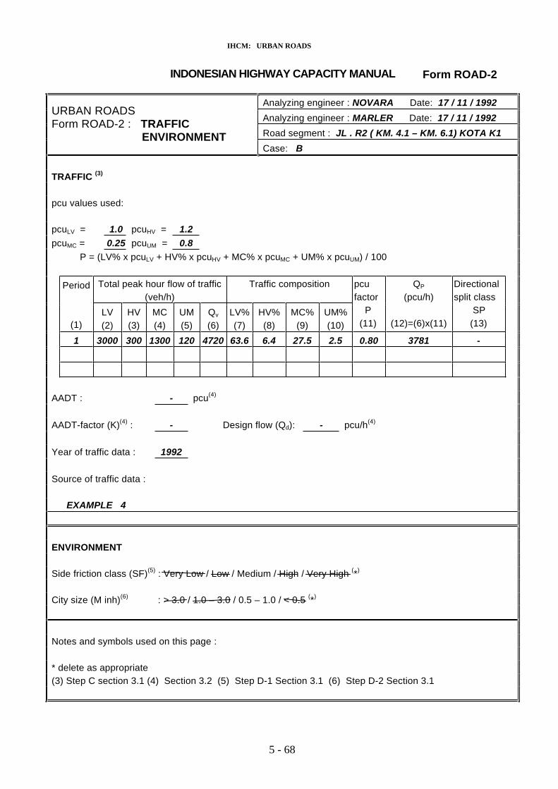
IHCM: URBAN ROADS
INDONESIAN HIGHWAY CAPACITY MANUAL Form ROAD-2
Analyzing engineer : NOVARA Date: 17 / 11 / 1992Analyzing engineer : MARLER Date: 17 / 11 / 1992Road segment : JL . R2 ( KM. 4.1 – KM. 6.1) KOTA K1
URBAN ROADS Form ROAD-2 : TRAFFIC
ENVIRONMENTCase: B
TRAFFIC (3)
pcu values used:
pcuLV = 1.0 pcuHV = 1.2pcuMC = 0.25 pcuUM = 0.8
P = (LV% x pcuLV + HV% x pcuHV + MC% x pcuMC + UM% x pcuUM) / 100
Total peak hour flow of traffic(veh/h)
Traffic compositionPeriod
(1)LV(2)
HV(3)
MC(4)
UM(5)
Qv
(6)LV%(7)
HV%(8)
MC%(9)
UM%(10)
pcufactor P (11)
QP
(pcu/h)
(12)=(6)x(11)
Directionalsplit class SP (13)
1 3000 300 1300 120 4720 63.6 6.4 27.5 2.5 0.80 3781 -
AADT : - pcu(4)
AADT-factor (K)(4) : - Design flow (Qd): - pcu/h(4)
Year of traffic data : 1992
Source of traffic data :
EXAMPLE 4
ENVIRONMENT
Side friction class (SF)(5) : Very Low / Low / Medium / High / Very High (*)
City size (M inh)(6) : > 3.0 / 1.0 – 3.0 / 0.5 – 1.0 / < 0.5 (*)
Notes and symbols used on this page :
* delete as appropriate(3) Step C section 3.1 (4) Section 3.2 (5) Step D-1 Section 3.1 (6) Step D-2 Section 3.1
5 - 68

IHCM: URBAN ROADS
INDONESIAN HIGHWAY CAPACITY MANUAL Form ROAD-3
Analyzing engineer : NOVARA Date: 3 / 12 / 1992Analyzing engineer : MARLER Date: 10 / 12 / 1992Road segment : JL . R4 ( KM. 5.7 – KM. 8.3) KOTA K4
URBAN ROADS Form ROAD-3 : ANALYSIS
RESULT COMMENTS Case: a
ANALYSIS(7)
C = CO x FW x FKS x FSP x FSF x FCS
V = VO x 0.5 [ 1 + ( 1 - DS ) 0.5 ]
Alternative
(1)
Basecapacity
CO
(pcu/h)Table E-1:1
(2)
Carriagewaywitdh
adjustmentfactor
FW
Table E-2:1
(3)
Kerb andshoulder adjust-
ment factorFKS
Table E-3:1 orE-3:2
(4)
Directionalsplit or median
adjustmentfactorFSP
Table E-4:1 orE-4:2
(5)
SideFriction
adjustnebtfactorFSF
Table E-5:1
(6)
City sizeadjustment
factorFCS
Table E-6:1
(7)1 5700 0.85 0.96 0.98 0.97 0.862 5700 0.85 0.96 0.98 0.97 0.863 5700 0.85 0.96 0.98 0.97 0.86
Capacity(8)
CO
(pcu/h)
(8)
Actual ordesign flowQp = or Qd
(pcu/h)
(9)
Degree of saturation(9)
DS
(10)
Free flowspeed(10)
VO
(km/h)Figure E-9:1 to
E-9:12(11)
Travelspeed(10)
V(km/h)
(12)
Avaragejourneytime (11)
(sec/km)
(13)
Sectionjourneytime(11)
TT(sec)
(14)3802 3781 0.99 51.5 28.3 - -4199 3781 0.90 51.5 33.9 - -3802 3381 0.89 51.5 34.3 - -
RESULTS(12) Alternative 1 Alternative 2 Alternative 3Actual or design flow (Qp or qd) (pcu/h) : 3781 3781 3381Capacity (C) (pcu/h) : 3802 4199 3802Ratio of flow to capacity (DS) : 0.99 0.90 0.89Estimated average speed (km/h) : 28 34 34Estimated average journey time (sec/km) : - - -Section journey time (sec) : - - -
COMMENTS(13)
alt. 1 : existing conditions ; alt. 2 : the warungs were removedalt. 3 : all angkutan kota were moved to another parallel routeNotes amd symbols used on this page
(7) Step E Section 3.1 (8) Step E-7 Section 3.1 (9) Step E-8 Section 3.1 (10) Step E-9 Section 3.1(11) Step E-10 Section 3.1 (12) Step E-11 Section 3.1 (13) Step E-12 Section 3.1
5 - 69
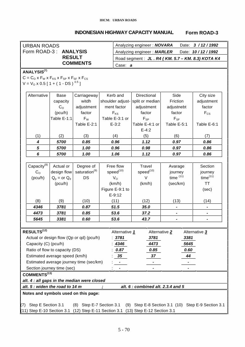
IHCM: URBAN ROADS
INDONESIAN HIGHWAY CAPACITY MANUAL Form ROAD-3
Analyzing engineer : NOVARA Date: 3 / 12 / 1992Analyzing engineer : MARLER Date: 10 / 12 / 1992Road segment : JL . R4 ( KM. 5.7 – KM. 8.3) KOTA K4
URBAN ROADS Form ROAD-3 : ANALYSIS
RESULT COMMENTS Case: a
ANALYSIS(7)
C = CO x FW x FKS x FSP x FSF x FCS
V = VO x 0.5 [ 1 + ( 1 - DS ) 0.5 ]
Alternative
(1)
Basecapacity
CO
(pcu/h)Table E-1:1
(2)
Carriagewaywitdh
adjustmentfactor
FW
Table E-2:1
(3)
Kerb andshoulder adjust-
ment factorFKS
Table E-3:1 orE-3:2
(4)
Directionalsplit or median
adjustmentfactorFSP
Table E-4:1 orE-4:2
(5)
SideFriction
adjustnebtfactorFSF
Table E-5:1
(6)
City sizeadjustment
factorFCS
Table E-6:1
(7)4 5700 0.85 0.96 1.12 0.97 0.865 5700 1.00 0.96 0.98 0.97 0.866 5700 1.00 1.06 1.12 0.97 0.86
Capacity(8)
CO
(pcu/h)
(8)
Actual ordesign flowQp = or Qd
(pcu/h)
(9)
Degree of saturation(9)
(10)
Free flowspeed(10)
VO
(km/h)Figure E-9:1 to
(11)
Travelspeed(10)
V
(12)
journeytime (11)
(sec/km)
Sectionjourneytime(11)
(14)
DS
E-9:12
(km/h)
Avarage
(13)
TT(sec)
4346 3781 0.87 51.5 35.0 - -4473 3781 0.85 53.6 37.2 - -5645 3381 0.60 53.6 43.7 - -
RESULTS(12) Alternative 1 Alternative 2 Alternative 3Actual or design flow (Qp or qd) (pcu/h) : 3781 3781 3381Capacity (C) (pcu/h) : 4346 4473 5645Ratio of flow to capacity (DS) : 0.87 0.85 0.60Estimated average speed (km/h) : 37 4435Estimated average journey time (sec/km) : - - -Section journey time (sec) : - - -
COMMENTS(13)
alt. 4 : all gaps in the median were closedalt. 5 : widen the road to 14 m ; alt. 6 : combined alt. 2.3.4 and 5Notes and symbols used on this page:
(7) Step E Section 3.1 (8) Step E-7 Section 3.1 (9) Step E-8 Section 3.1 (10) Step E-9 Section 3.1(11) Step E-10 Section 3.1 (12) Step E-11 Section 3.1 (13) Step E-12 Section 3.1
5 - 70

IHCM: URBAN ROADS
5.5 EXAMPLE 5 : ANALYSIS OF FOUR-LANE TWO-WAY ROAD, FOR USE INA NETWORK ANALYSIS
Kerbed, no obstructions within 2.0 m on either side
City size < 500,000 in h.
Questions:
Solution:
Geometry : 14 m
No medianSegment length : 2 km
Traffic : Directional split of 70 - 30
Environment : Few pedestrians Few angkutan kota Few vehicles entering/leaving premises
The peak traffic flow is expected to be 3000 pcu/h
1. What is the average travel time along the segment ?
a. in sec
b. in sec/km
See Figure 5.5:1 to 5.5:3.
5 - 71

IHCM: URBAN ROADS
INDONESIAN HIGHWAY CAPACITY MANUAL Form ROAD-1
URBAN ROADSForm ROAD-1 : GENERAL
GEOMETRYGENERAL(1)
Road segment identification (site name/section/city):JL. R5 BETWEEN KM. 5.3 AND KM. 7.3 KOTA K5
Segment length (L): 2.0 kmAnalyzing engineer: NOVARA Date: day 12 month 1 year 1993Checking engineer: MARLER Date: day 17 month 1 year 1993Case: A
GEOMETRY(2)
Shoulder / ke oulder and kerb (*)rb / sh
Difference between levels of shoulder and carriageway : < 10 cm; considered as shouder> 10 cm; considered as shouder = 0 m
Median / no-median (*) : only considered for four-lane two-way roads
Dimensions:Side A : m-
{ Effective shoulder witdh (WSe)Or distance from kerb to obstruction (WKe) : > 2 m
Effective carriageway witdh (WCe) : m14
: mSide B
{ Effective shoulder witdh (WSe)Or distance from kerb to obstruction (WKe) : > 2 m
If median:Median witdh (W M) : - mMedian continuity: no gaps / few gaps / frequent gaps (*)
If shoulder:Avarage effective shoulder witdh (WSe) : - m
If kerb: Avarage distance fromkerb to obstruction (WKe): > 2 m
Source of geometric data :
EXAMPLE 5
Notes and symbols used on this page :* delete as appropriate(1) Step A Section 3.1(2) Step B Section 3.1
5 - 72

IHCM: URBAN ROADS
Form ROAD-2INDONESIAN HIGHWAY CAPACITY MANUAL
Analyzing engineer : NOVARA Date: 17 / 11 / 1992Analyzing engineer : MARLER Date: 17 / 11 / 1992Road segment : JL . R5 ( KM. 5.3 – KM. 7.3) KOTA K5
URBAN ROADS Form ROAD-2 : TRAFFIC
ENVIRONMENTCase: a
TRAFFIC (3)
pcu values used:
pcuLV = - pcuHV = -pcuMC = - pcuUM = -
P = (LV% x pcuLV + HV% x pcuHV + MC% x pcuMC + UM% x pcuUM) / 100
Total peak hour flow of traffic(veh/h)
Traffic compositionPeriod
(2)HV(3) (5)
Qv
(6)MC%
(9) (10)
factor
(11)
QP
(12)=(6)x(11)
split class SP (13) (1)
LV MC(4)
UM LV%(7)
HV%(8)
UM%
pcu
P (pcu/h)
Directional
1 - - - - - - - - - - 3000 70 / 30
AADT : - pcu(4)
AADT-factor (K)(4) : - Design flow (Qd): - pcu/h(4)
Year of traffic data : 1992
Source of traffic data :
EXAMPLE 5
ENVIRONMENT
Side friction class (SF)(5) Low / Medi ry High (*) : Very Low / um / High / Ve
City size (M inh)(6) : > 5 (*)3.0 / 1.0 – 3.0 / 0.5 – 1.0 / < 0.
Notes and symbols used on this page :
* delete as appropriate(3) Step C section 3.1 (4) Section 3.2 (5) Step D-1 Section 3.1 (6) Step D-2 Section 3.1
5 - 73

IHCM: URBAN ROADS
INDONESIAN HIGHWAY CAPACITY MANUAL Form ROAD-3
Analyzing engineer : NOVARA Date: 3 / 12 / 1992Analyzing engineer : MARLER Date: 10 / 12 / 1992Road segment : JL . R5 ( KM. 5.3 – KM. 7.3) KOTA K5
URBAN ROADS Form ROAD-3 : ANALYSIS
RESULT COMMENTS Case: a
ANALYSIS(7)
C = CO x FW x FKS x FSP x FSF x FCS
V = VO x 0.5 [ 1 + ( 1 - DS ) 0.5 ]
Alternative
(1)
capacityCO
(pcu/h)
witdh
factorFW
shoulder adjust-ment factor
FKS
(4)
split or medianadjustment
factorFSP
Table E-4:1 orE-4:2
Side
adjustnebtfactorFSF
(6)
factorFCS
Base
Table E-1:1
(2)
Carriageway
adjustment
Table E-2:1
(3)
Kerb and
Table E-3:1 orE-3:2
Directional
(5)
Friction
Table E-5:1
City sizeadjustment
Table E-6:1
(7)1 5700 1.00 1.00 0.94 1.00 0.80
Capacity(8)
CO
(8)
design flowQp = or Qd
(pcu/h)
Degree of saturation(9)
(10)
Free flowspeed(10)
VO
(km/h)Figure E-9:1 to
E-9:12(11)
Travelspeed(10)
V(km/h)
journeytime (11)
(13)
journeytime(11)(pcu/h)
Actual or
(9)
DS
(12)
Avarage
(sec/km)
Section
TT(sec)
(14)4286 3000 0.70 56.4 43.6 82.5 165.0
RESULTS(12) Alternative 1 Alternative _ Alternative _Actual or design flow (Qp or qd) (pcu/h) : 3000Capacity (C) (pcu/h) : 4286Ratio of flow to capacity (DS) : 0.70Estimated average speed (km/h) : 44Estimated average journey time (sec/km) : 83Section journey time (sec) : 165
COMMENTS(13)
Notes and symbols used on this page:
(7) Step E Section 3.1 (8) Step E-7 Section 3.1 (9) Step E-8 Section 3.1 (10) Step E-9 Section 3.1(11) Step E-10 Section 3.1 (12) Step E-11 Section 3.1 (13) Step E-12 Section 3.1
5 - 74

IHCM: URBAN ROADS
5.6 EXAMPLE 6: DESIGN OF A NEW ROAD
(distance to obstructions/effective shoulder width > 2.0 m)- A median or no median (your choice)
- Medium friction
A new at-grade road of standard design is to be built in Sukabumi. The predicted peak hour flow forthe design year is 1700 pcu.
Standard design:
- 3.5 metre lanes- Kerb or shoulder (your choice)
Questions:
1. How many standard lanes are needed ?
Assume
- Directional split of 60 - 40
- A Q/C ratio of 0.6 or lower is required for the design year
Solution:
See Figure 5.6:1 to 5.6:3.
5 - 75

IHCM: URBAN ROADS
Form ROAD-1
GEOMETRY
INDONESIAN HIGHWAY CAPACITY MANUAL
URBAN ROADSForm ROAD-1 : GENERAL
GENERAL(1)
Road segment identification (site name/section/city):JL. R6 BETWEEN KM. 13.2 AND KM. 15.7 KOTA SUKABUMI
Segment length (L): 2.5 kmAnalyzing engineer: NOVARA Date: day 4 month 12 year 1993Checking engineer: MARLER Date: day 10 month 12 year 1993Case: A
GEOMETRY(2)
Shoulder / ke oulder and kerb (*)rb / sh
Difference between levels of shoulder and carriageway : < 10 cm; considered as shouder> 10 cm; considered as shouder = 0 m
Median / no-median (*) : only considered for four-lane two-way roads
Dimensions:Side A : m> 2
{ Effective shoulder witdh (WSe)Or distance from kerb to obstruction (WKe) : - m
Effective carriageway witdh (WCe) : m3x3.5
: > 2 mSide B
{ Effective shoulder witdh (WSe)Or distance from kerb to obstruction (WKe) : - m
If median:Median witdh (W M) : - mMedian continuity: no gaps / few gaps / frequent gaps (*)
If shoulder:Avarage effective shoulder witdh (WSe) : > 2 m
If kerb: Avarage distance fromkerb to obstruction (WKe): - m
Source of geometric data :
EXAMPLE 6
Notes and symbols used on this page :* delete as appropriate(1) Step A Section 3.1(2) Step B Section 3.1
5 - 76

IHCM: URBAN ROADS
INDONESIAN HIGHWAY CAPACITY MANUAL Form ROAD-2
Analyzing engineer : NOVARA Date: 4 / 12 / 1992Analyzing engineer : MARLER Date: 10 / 12 / 1992Road segment :JL . R6 ( KM. 13.3 – KM. 15.3)SUKABUMI
URBAN ROADS Form ROAD-2 : TRAFFIC
ENVIRONMENTCase: a
TRAFFIC (3)
pcu values used:
pcuLV = - pcuHV = -pcuMC = - pcuUM = -
P = (LV% x pcuLV + HV% x pcuHV + MC% x pcuMC + UM% x pcuUM) / 100
Total peak hour flow of traffic(veh/h)
Traffic compositionPeriod
LV(2) (3)
MC(4) (5)
Qv
(6)LV%(7) (8)
MC%(9) (10)
pcufactor
(11)
QP
(pcu/h)
(12)=(6)x(11)
split class SP (13) (1)
HV UM HV% UM% P
Directional
1 - - - 60 / 40- - - - - - - 1700
AADT : - pcu(4)
AADT-factor (K)(4) : - Design flow (Qd): - pcu/h(4)
Year of traffic data : 1992
Source of traffic data :
EXAMPLE 6
ENVIRONMENT
Side friction class (SF)(5) um / Hi ry High (*) : Very Low / Low / Medi gh / Ve
City size (M inh)(6) : > 5 (*)3.0 / 1.0 – 3.0 / 0.5 – 1.0 / < 0.
Notes and symbols used on this page :
* delete as appropriate(3) Step C section 3.1 (4) Section 3.2 (5) Step D-1 Section 3.1 (6) Step D-2 Section 3.1
5 - 77

IHCM: URBAN ROADS
INDONESIAN HIGHWAY CAPACITY MANUAL Form ROAD-3
Analyzing engineer : NOVARA Date: 4 / 12 / 1992Analyzing engineer : MARLER Date: 10 / 12 / 1992Road segment : JL . R5 ( KM. 5.3 – KM. 7.3)SUKABUMI
URBAN ROADS Form ROAD-3 : ANALYSIS
RESULT COMMENTS Case: a
ANALYSIS(7)
C = CO x FW x FKS x FSP x FSF x FCS
V = VO x 0.5 [ 1 + ( 1 - DS ) 0.5 ]
Alternativecapacity
CO
Table E-1:1factor
FW
Kerb andshoulder adjust-
ment factorFKS
split or medianadjustment
factorFSP
factorFSF
Table E-5:1
(6)
factorFCS
(7)(1)
Base
(pcu/h)
(2)
Carriagewaywitdh
adjustment
Table E-2:1
(3)
Table E-3:1 orE-3:2
(4)
Directional
Table E-4:1 orE-4:2
(5)
SideFriction
adjustnebt
City sizeadjustment
Table E-6:1
1 5700 0.63 1.06 0.97 0.97 0.80
Capacity(8)
CO design flowQp = or Qd
Degree of saturation(9)
DS
Free flowspeed(10)
VO
Figure E-9:1 toE-9:12
Travelspeed(10)
Avaragejourneytime (11)
(13)
journeytime(11)
TT(sec)
(14)
(pcu/h)
(8)
Actual or
(pcu/h)
(9) (10)
(km/h)
(11)
V(km/h)
(12)
(sec/km)
Section
2865 1700 0.59 - - --
RESULTS(12) Alternative 1 Alternative _ Alternative _Actual or design flow (Qp or qd) (pcu/h) : 1700Capacity (C) (pcu/h) : 2865Ratio of flow to capacity (DS) : 0.59Estimated average speed (km/h) : -Estimated average journey time (sec/km) : -Section journey time (sec) : -
COMMENTS(13) Three lanes will therefore carry the traffic at the required Q/C ratio of 0.6 or less ,but three – lane roads may be dangerous , so four-lane road may be better
Notes and symbols used on this page:
(7) Step E Section 3.1 (8) Step E-7 Section 3.1 (9) Step E-8 Section 3.1 (10) Step E-9 Section 3.1(11) Step E-10 Section 3.1 (12) Step E-11 Section 3.1 (13) Step E-12 Section 3.1
5 - 78

IHCM: URBAN ROADS
5.7 EXAMPLE 7: PLANNING
A new road is being planned. The predicted AADT is 30,000 pcu. The road must operate at a Q/C ratio of 0.6 or less in the design year.
Questions:
1. Will a 4-lane road be sufficient ?
Assume :
- Standard lane witdh of 3.5 m- kerb witdh > 2.0 m to obstructions - No median- Directional split of 60 – 40 - Medium friction- City size 1.0 – 3.0 M
Solution:
The assumptions used for planning four-lane two-way roads are the same as the assumedconditions given in Section 3.2.2, so no worksheet is needed. Relating the predicted AADT (30,000 pcu) to the corresponding values shown in Table 3.2.2:1 gives the Q/C ratio is about 0.53, so a four-lane road will be sufficient.
5 - 79

IHCM: URBAN ROADS
5.8 EXAMPLE 8: OPERATIONAL ANALYSIS OF URBAN MOTORWAYS
Traffic : - Side A: QLV = 2700 veh/hQHV = 800 veh/h
- Side B: QLV = 3200 veh/hQHV = 600 veh/h
Solution:
See Figure 5.8:1 and 5.8:2.
Geometry : 7.5 m carriageway width (both side)1.0 m effective shoulder on side A2.0 m effective shoulder on side B2.0 m median width
Environment : City size > 3.0 M Questions:
1. What peak hour speed will be the road operate at ?
2. What is the flow/capacity ratio ?
5 - 80

IHCM: URBAN ROADS
Form ROAD-4INDONESIAN HIGHWAY CAPACITY MANUAL
TRAFFIC
URBAN ROADSForm ROAD-1 : GENERAL
GEOMETRY
GENERAL(1)
Road segment identification (site name/section/city):JL. M.T Haryono between km 5.7 and km 9.2 kota Jakarta
Segment length (L): 3.5 kmAnalyzing engineer: NOVARA Date: day17 month 11 year 1993Checking engineer: MARLER Date: day20 month 11 year 1993Case: aGEOMETRY(2)
Dimensions:Side A: Effective left shoulder witdh (WSe) : m1.0
Side A Effective carriageway witdh (WCe) : 7.5 m
median witdh (WM) : 2.0 m
Side B: Side B Effective carriageway witdh (WCe) : 7.5 m
Effective left shoulder witdh (WSe) m: 2.0Source of geometric data:
EXAMPLE 8
TRAFFIC (3)
pcu values used: pcuLV = 1.0 pcuHV = 1.2P = (LV% x pcuLV + HV% x pcuHV ) / 100
(veh/h)Total peak hour flow of traffic Traffic compositionSide
(1)
Periode
(4)Q P
(8)
Q
(2) LV(3)
HV v(5)
LV%(6)
HV(7)
pcufactor
p(pcu/h)
(9)=(5)x(8)A 1.051 2700 800 3500 77.1 22.9 3660
B 1 3200 600 3800 84.2 15.8 1.03 3920
AADT: - pcu (4)
AADT-factor (K) (4) : - Design flow (Qd): - pcu/h (4)
Year of traffic data : 1992Source of traffic data :
EXAMPLE 8
Notes and symbols used on this page :* delete as appropriate(1) Step A Section 4.1 (2) Step B Section 4.1 (3) Step C Section 4.1 (4) Section 4.2
5 - 81

IHCM: URBAN ROADS
INDONESIAN HIGHWAY CAPACITY MANUAL Form ROAD-5
Analyzing engineer : NOVARA Date: 4 / 12 / 1992Analyzing engineer : MARLER Date: 10 / 12 / 1992Road segment: Jl.M.T.Haryono (km 5.7-km 9.2) Jakarta
URBAN ROADS Form ROAD-3 : ANALYSIS
RESULT COMMENTS Case: a
ANALYSIS(5)
Side A :
Qi = 4600 x (Q/Co)i x FWSpeed
Vi
(1)pcu/h Table 4.1:1(km/h)
(2) (3) (4)Table D-1:1
(5)
75 = 4600 0.4070 = 4600 0.6165 3416 = 4600 0.75 0.9958 4053 = 4600 0.89 0.9945 4554
(Capacity)= 4600 1.00 0.99
Side B :
Qi = 4600 x (Q/Co)i x FWSpeed
Vi
(1) (3) (4) (5)(km/h)
(2)pcu/h Table 4.1:1 Table D-1:1
75 = 0.40460070 = 4600 0.6165 3485 = 0.754600 1.0158 1.014135 = 4600 0.8945 4646
(Capacity)= 4600 1.00 1.01
RESULTS (10) Side A Side B Actual or design flow (Qp or Qd) (pcu/h) : 3660 3920Capacity (C) (pcu/h) (6) : 4554 4646Ratio of flow to capacity (DS) (7) : 0.840.80Estimated average speed (km/h) (8) : 62 60Estimated average journey time (sec/km) (9) -: -Section journey time (sec) (9) : - -
COMMENTS (11)
Notes and symbols used on this page:* delete as appropriate
(5) Step D Section 4.1 (6) Step D-2 Secton 4.1 (7) Step D-3 Section 4.1(8) Step D-4 Section 4.1 (9) Step D-5 Section 4.1 (10) Step D-6 Section 4.1(11) Step D-7 Section 4.1
5 - 82

IHCM: URBAN ROADS
6. LITERATURE REFERENCE
R1. TRB Highway Capacity Manual. Transportation Research Board, Special Report 209; Washington DC. USA 1985
R2. May, A.D. Traffic Flow Fundamentals.Prentice-Hal, Inc; 1990.
R3. Easa, S.M. Generalized Procedure for Estimating Single- and Two-Regime Traffic-flow Models.Transportation Research Records 772; WashingtonD.C USA 1987
R4. Hoban, C.J. Evaluating Traffic Capacity and Improvements to Road Geometry.World Bank Technical Paper Number 74; WashingtonD.C. USA 1987.
R5. OECD Traffic Capacity of Major Routes. Road TransportResearch; 1983.
R6. Brannolte,U. Highway Capacity and Level of Service.(editor) Proceedings of International Symposium on
Highway Capacity, Karlsruhe; Rotterdam Netherlands 1991.
R7. McShane, W.R. Traffic Engineering. Roess, R.P. Prentice-Hall, Inc; 1990.
R8. Black, J.A., Land Use along Arterial Roads: Friction and Westerman, H.L. Impact. Blinkhorn, L. The University of New South Wales; 1988. McKittrick, J.
R9. Pfefer, R.C. First New Chapter for the Highway CapacityManual. ITE Journal; September 1992.
R10. TRB Highway Capacity Manual (Revised Chapter 7:Multilane Rural and Suburban Highways).Transportation Research Board; Washington D.C. 1992.
R11. NAASRA Guide to Traffic Engineering Practice. NationalAssociation of Australian State Road Authorities;1988.
5 - 83

IHCM: URBAN ROADS
R12. Negara, I.N.W. Speed-Volume Relationship on Congested Roads in Bandung.Msc. Thesis S2-STJR ITB; 1991.
R13. Directorate General Highway Capacity in Indonesia. of Highways Highway Betterment Services Screening Feasibility
Project, Special Report, ENEX of New Zealand,Consortium 346; 1979.
R14. Nusrihardono, B.B.A. Speed-Flow Relationship in Bandung Urban Area. Msc. Thesis S2-STIR ITB; 1984.
R15. Directorate General Standard Specification for Geometric Design of of Highways Urban Roads.
Ministry of Public Works; 1988.
R16. Government of Indonesia Undang-undang Republik Indonesia No. 13 Tahun 1980tentang Jalan.
R17. Government of Indonesia Peraturan Pemerintah Republik Indonesia No. 8 Tahun 1990 tentang Jalan Tol.
5 - 84

IHCM: URBAN ROADS Appendix 5:1
INDONESIAN HIGHWAY CAPACITY MANUAL Form ROAD-1
URBAN ROADSForm ROAD-1 : GENERAL
GEOMETRYGENERAL(1)
Road segment identification (site name/section/city):
Segment length (L): kmAnalyzing engineer: Date: day month year 1993Checking engineer: Date: day month year 1993Case:
GEOMETRY(2)
Shoulder / kerb / Shoulder and kerb (*)
Difference between levels of shoulder and carriageway : < 10 cm; considered as shouder> 10 cm; considered as shouder = 0 m
Median / no-median (*) : only considered for four-lane two-way roads
Dimensions:Side A : m
{ Effective shoulder witdh (WSe)Or distance from kerb to obstruction (WKe) : m
Effective carriageway witdh (WCe) : m
: mSide B
{ Effective shoulder witdh (WSe)Or distance from kerb to obstruction (WKe) : m
If median:Median witdh (W M) : mMedian continuity: no gaps / few gaps / frequent gaps (*)
If shoulder:Avarage effective shoulder witdh (WSe) : m
If kerb: Avarage distance fromkerb to obstruction (WKe): m
Source of geometric data :
Notes and symbols used on this page :* delete as appropriate(1) Step A Section 3.1(2) Step B Section 3.1
5 - 85

IHCM: URBAN ROADS Appendix 5:1
INDONESIAN HIGHWAY CAPACITY MANUAL Form ROAD-2
Analyzing engineer : Date:Analyzing engineer : Date:Road segment :
URBAN ROADS Form ROAD-2 : TRAFFIC
Case: ENVIRONMENT
TRAFFIC (3)
pcu values used:
pcuLV = pcuHV =pcuMC = pcuUM =
P = (LV% x pcuLV + HV% x pcuHV + MC% x pcuMC + UM% x pcuUM) / 100
Total peak hour flow of traffic(veh/h)
Traffic compositionPeriod
UM(5)
Qv HV% MC% (11)
QP Directional
(1)LV(2)
HV(3)
MC(4) (6)
LV%(7) (8) (9)
UM%(10)
pcufactor P
(pcu/h)
(12)=(6)x(11)
split class SP (13)
AADT : pcu(4)
AADT-factor (K)(4) : Design flow (Qd): pcu/h(4)
Year of traffic data :
Source of traffic data :
ENVIRONMENT
Side friction class (SF)(5) : Very Low / Low / Medium / High / Very High (*)
City size (M inh)(6) : > 3.0 / 1.0 – 3.0 / 0.5 – 1.0 / < 0.5 (*)
Notes and symbols used on this page :
* delete as appropriate(3) Step C section 3.1 (4) Section 3.2 (5) Step D-1 Section 3.1 (6) Step D-2 Section 3.1
5 - 86

IHCM: URBAN ROADS Appendix 5:1
INDONESIAN HIGHWAY CAPACITY MANUAL Form ROAD-3
Analyzing engineer : Date:Analyzing engineer : Date:Road segment :
URBAN ROADS Form ROAD-3 : ANALYSIS
RESULT COMMENTS Case:
ANALYSIS(7)
C = CO x FW x FKS x FSP x FSF x FCS
V = VO x 0.5 [ 1 + ( 1 - DS ) 0.5 ]
Alternative Basecapacity
CO
Table E-1:1factor
FW
(3)
shoulder adjust-ment factor
FKS
split or medianadjustment
factorFSP
(5)
factorFSF
factorFCS
Table E-6:1
(7)(1)
(pcu/h)
(2)
Carriagewaywitdh
adjustment
Table E-2:1
Kerb and
Table E-3:1 orE-3:2
(4)
Directional
Table E-4:1 orE-4:2
SideFriction
adjustnebt
Table E-5:1
(6)
City sizeadjustment
Capacity(8)
CO
Actual ordesign flowQp = or Qd
Degree of saturation(9)
Free flowspeed(10)
VO
(11)
Travelspeed(10)
V
(12)
Avaragejourneytime (11)
(13)
Sectionjourneytime(11)
TT(sec)
(14)
(pcu/h)
(8)
(pcu/h)
(9)
DS
(10)
(km/h)Figure E-9:1 to
E-9:12
(km/h) (sec/km)
RESULTS(12) Alternative _ Alternative _ Alternative _Actual or design flow (Qp or qd) (pcu/h) :Capacity (C) (pcu/h) :Ratio of flow to capacity (DS) :Estimated average speed (km/h) :Estimated average journey time (sec/km) :Section journey time (sec) :
COMMENTS(13)
Notes and symbols used on this page:
(7) Step E Section 3.1 (8) Step E-7 Section 3.1 (9) Step E-8 Section 3.1 (10) Step E-9 Section 3.1(11) Step E-10 Section 3.1 (12) Step E-11 Section 3.1 (13) Step E-12 Section 3.1
5 - 87

IHCM: URBAN ROADS Appendix 5:1
Form ROAD-4
URBAN ROADSForm ROAD-1 : GENERAL
GEOMETRY TRAFFIC
INDONESIAN HIGHWAY CAPACITY MANUAL
GENERAL(1)
Road segment identification (site name/section/city):
Segment length (L): kmAnalyzing engineer: Date: day month year ______Checking engineer: Date: day month year ______Case:GEOMETRY(2)
Dimensions:Side A: Effective left shoulder witdh (WSe) : m
Side A Effective carriageway witdh (WCe) : m
median witdh (WM) : m
Side B: Side B Effective carriageway witdh (WCe) : m
Effective left shoulder witdh (WSe) : mSource of geometric data:
TRAFFIC (3)
pcu values used: pcuLV = 1.0 pcuHV = 1.2P = (LV% x pcuLV + HV% x pcuHV ) / 100
Total peak hour flow of traffic(veh/h)
Traffic composition
LV(3)
HV(4)
Qv(5)
LV%(6)
HV(7)
factor P (8)
Qp(pcu/h)
(9)=(5)x(8)
Side
(1)
Periode
(2)
pcu
A
B
AADT: pcu (4)
AADT-factor (K) (4) : Design flow (Qd): pcu/h (4)
Year of traffic data : Source of traffic data :
Notes and symbols used on this page :* delete as appropriate(1) Step A Section 4.1 (2) Step B Section 4.1 (3) Step C Section 4.1 (4) Section 4.2
5 - 88

IHCM: URBAN ROADS
Form ROAD-5INDONESIAN HIGHWAY CAPACITY MANUAL
Analyzing engineer : Date:Analyzing engineer : Date:Road segment:
URBAN ROADS Form ROAD-3 : ANALYSIS
RESULT COMMENTS Case:
ANALYSIS(5)
Side A :
Qi = 4600 x (Q/Co)i x FWSpeed
Vi
(1)(km/h)
(2)pcu/h
(3)Table 4.1:1
(4)Table D-1:1
(5)
75 = 4600 0.4070 = 4600 0.6165 = 4600 0.7558 = 4600 0.8945
(Capacity)= 4600 1.00
Side B :
Qi = 4600 x (Q/Co)i x FWSpeed
Vi
(1)Table D-1:1(km/h)
(2)pcu/h
(3)Table 4.1:1
(4) (5)75 = 4600 0.4070 = 4600 0.6165 = 4600 0.7558 = 4600 0.8945
(Capacity)= 4600 1.00
RESULTS (10) Side A Side B Actual or design flow (Qp or Qd) (pcu/h) :Capacity (C) (pcu/h) (6) :Ratio of flow to capacity (DS) (7) :Estimated average speed (km/h) (8) :Estimated average journey time (sec/km) (9) :Section journey time (sec) (9) :
COMMENTS (11)
Notes and symbols used on this page:* delete as appropriate
(5) Step D Section 4.1 (6) Step D-2 Secton 4.1 (7) Step D-3 Section 4.1(8) Step D-4 Section 4.1 (9) Step D-5 Section 4.1 (10) Step D-6 Section 4.1(11) Step D-7 Section 4.1
5 - 89