individual attitudes toward corruption: do social effects...
TRANSCRIPT
Individual Attitudes Toward Corruption:Do Social Effects Matter?
Roberta GattiWorld Bank
Stefano PaternostroWorld Bank
Jamele RigoliniNYU and U. of Warwick
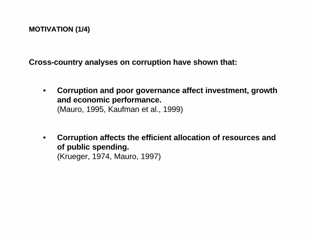
MOTIVATION (1/4)MOTIVATION (1/4)
Cross-country analyses on corruption have shown that:
• Corruption and poor governance affect investment, growth and economic performance.(Mauro, 1995, Kaufman et al., 1999)
• Corruption affects the efficient allocation of resources and of public spending.(Krueger, 1974, Mauro, 1997)
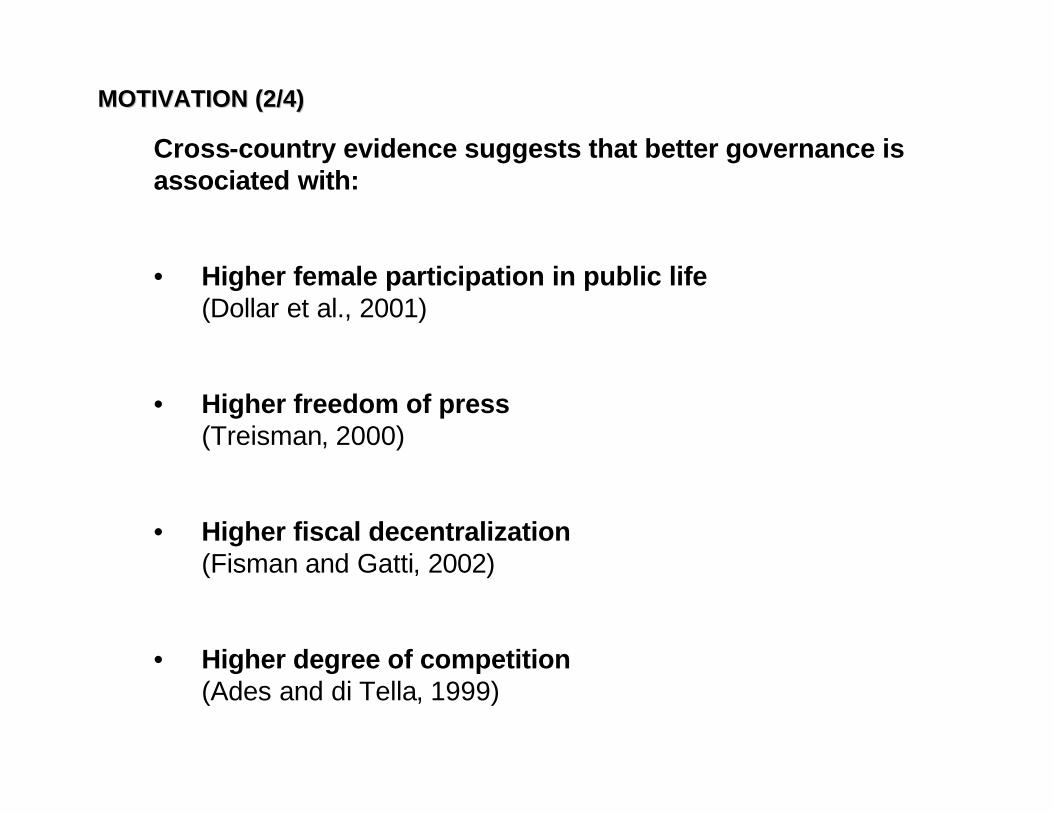
MOTIVATION (2/4)MOTIVATION (2/4)
Cross-country evidence suggests that better governance is associated with:
• Higher female participation in public life(Dollar et al., 2001)
• Higher freedom of press(Treisman, 2000)
• Higher fiscal decentralization(Fisman and Gatti, 2002)
• Higher degree of competition(Ades and di Tella, 1999)
MOTIVATION (3/4)MOTIVATION (3/4)
• Cross-country studies explain the macro-level correlates of corruption.
• But it is sometimes difficult to get rid of unobservables.
• Effective anti-corruption policies need to understand the micro-economics of corruption.
• Few studies, however, analyze the determinants of corruption at the individual level.
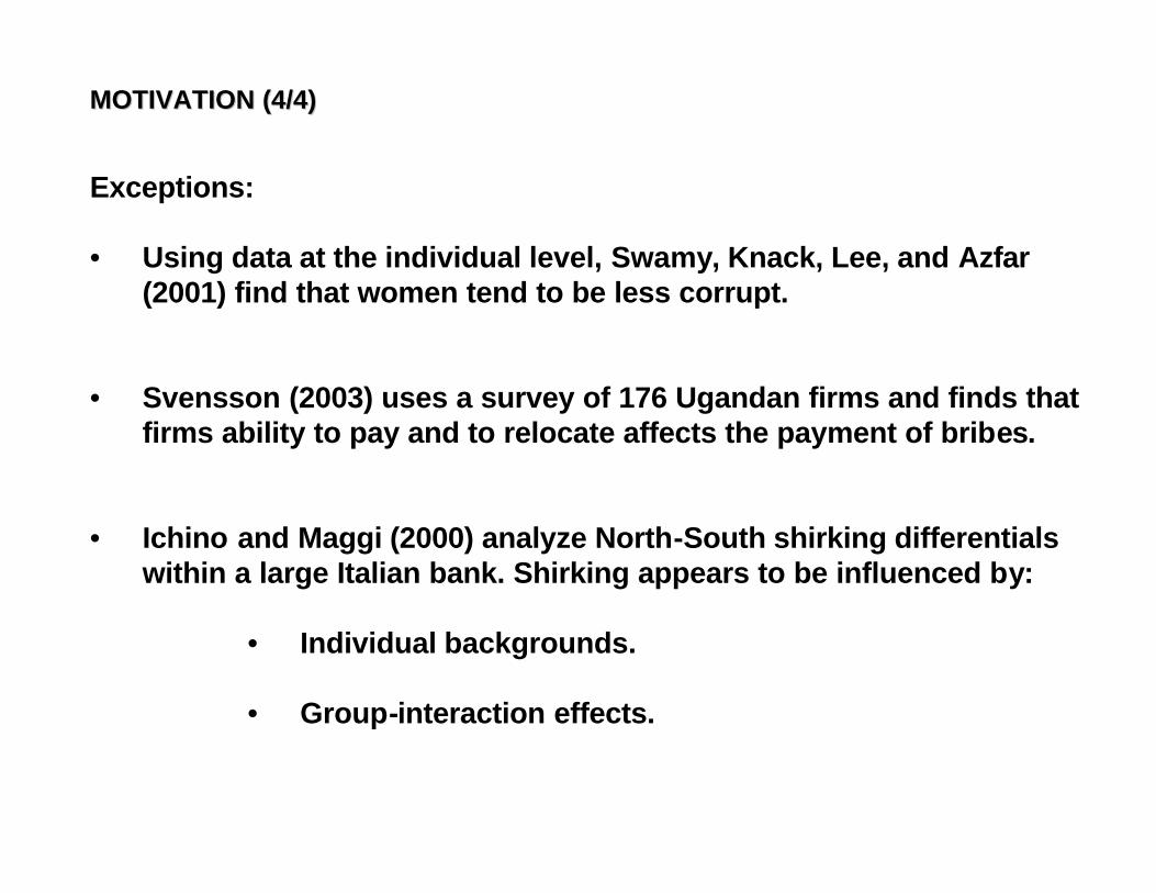
MOTIVATION (4/4)MOTIVATION (4/4)
Exceptions:
• Using data at the individual level, Swamy, Knack, Lee, and Azfar(2001) find that women tend to be less corrupt.
• Svensson (2003) uses a survey of 176 Ugandan firms and finds that firms ability to pay and to relocate affects the payment of bribes.
• Ichino and Maggi (2000) analyze North-South shirking differentials within a large Italian bank. Shirking appears to be influenced by:
• Individual backgrounds.
• Group-interaction effects.
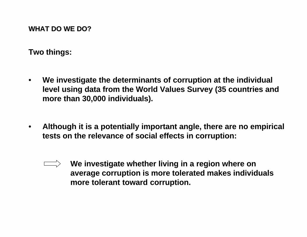
Two things:
• We investigate the determinants of corruption at the individual level using data from the World Values Survey (35 countries and more than 30,000 individuals).
• Although it is a potentially important angle, there are no empirical tests on the relevance of social effects in corruption:
We investigate whether living in a region where on average corruption is more tolerated makes individuals more tolerant toward corruption.
WHAT DO WE DO?WHAT DO WE DO?
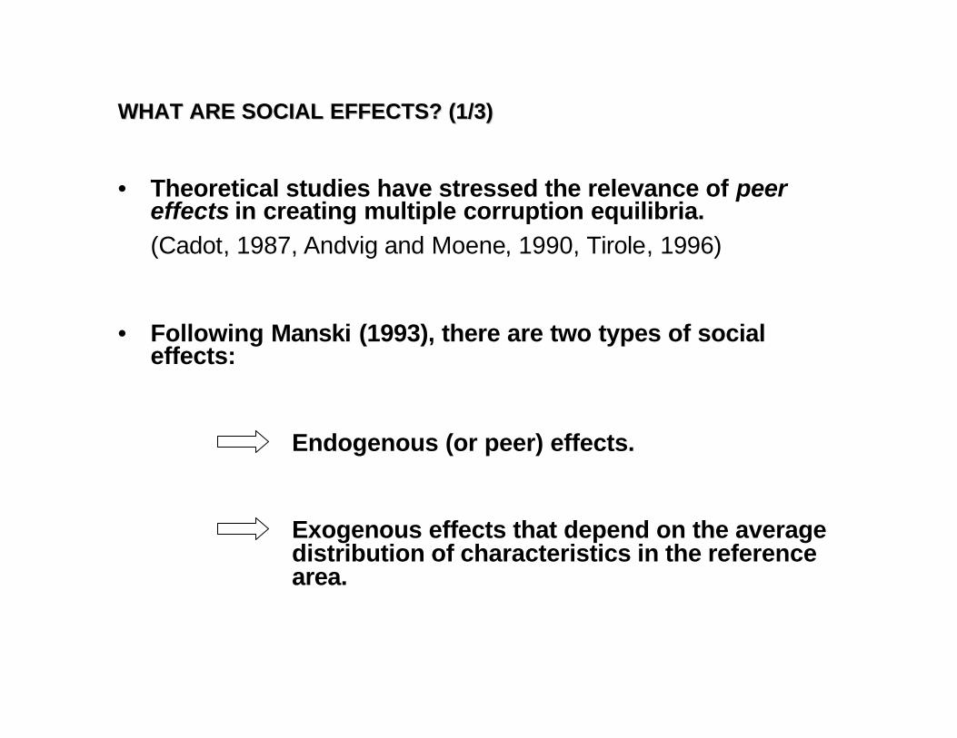
WHAT ARE SOCIAL EFFECTS? (1/3)WHAT ARE SOCIAL EFFECTS? (1/3)
• Theoretical studies have stressed the relevance of peer effects in creating multiple corruption equilibria.(Cadot, 1987, Andvig and Moene, 1990, Tirole, 1996)
• Following Manski (1993), there are two types of social effects:
Endogenous (or peer) effects.
Exogenous effects that depend on the average distribution of characteristics in the reference area.
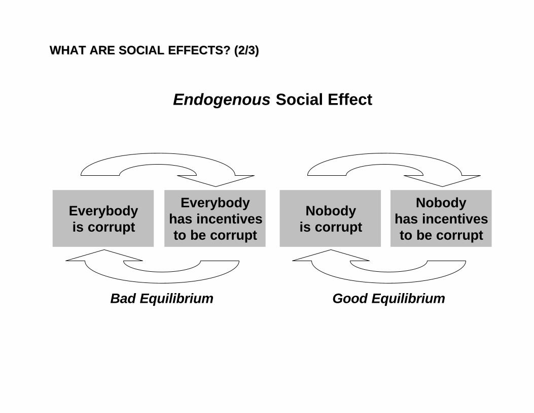
WHAT ARE SOCIAL EFFECTS? (2/3)WHAT ARE SOCIAL EFFECTS? (2/3)
Everybodyis corrupt
Everybodyhas incentivesto be corrupt
Nobodyis corrupt
Nobodyhas incentivesto be corrupt
Bad Equilibrium Good Equilibrium
Endogenous Social Effect
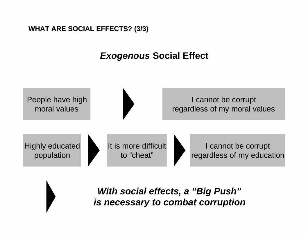
WHAT ARE SOCIAL EFFECTS? (3/3)WHAT ARE SOCIAL EFFECTS? (3/3)
People have highmoral values
I cannot be corruptregardless of my moral values
Highly educatedpopulation
It is more difficultto “cheat”
I cannot be corruptregardless of my education
Exogenous Social Effect
With social effects, a “Big Push”is necessary to combat corruption
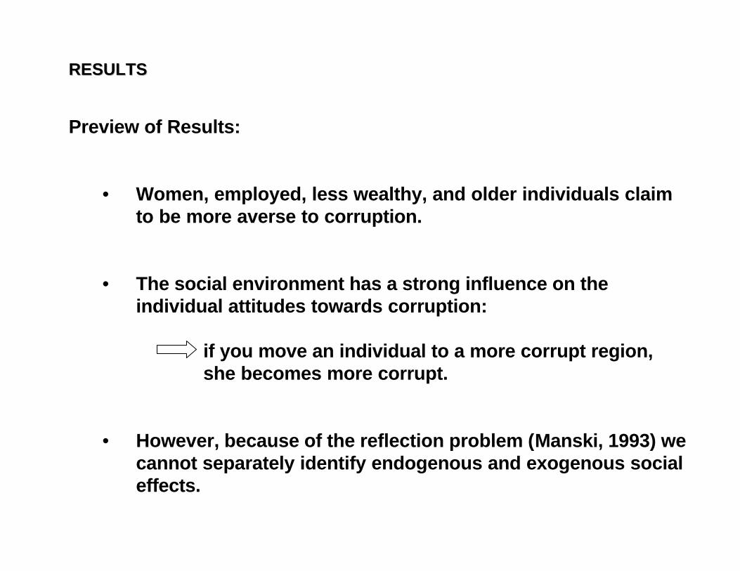
Preview of Results:
• Women, employed, less wealthy, and older individuals claim to be more averse to corruption.
• The social environment has a strong influence on the individual attitudes towards corruption:
if you move an individual to a more corrupt region, she becomes more corrupt.
• However, because of the reflection problem (Manski, 1993) we cannot separately identify endogenous and exogenous social effects.
RESULTSRESULTS
DATA (1/2)DATA (1/2)
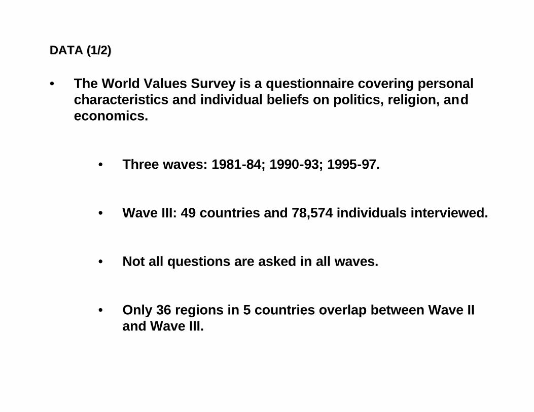
• The World Values Survey is a questionnaire covering personal characteristics and individual beliefs on politics, religion, and economics.
• Three waves: 1981-84; 1990-93; 1995-97.
• Wave III: 49 countries and 78,574 individuals interviewed.
• Not all questions are asked in all waves.
• Only 36 regions in 5 countries overlap between Wave II and Wave III.

DATASET (2/2)DATASET (2/2)
Previous works using the WVS:
• Knack and Keefer (1997) build indices of social capital.
• Swamy et al. (2001) analyze the women’s attitudes towards corruption.
• Guiso et al. (2002) look at the relationship between religion and socioeconomic attitudes.
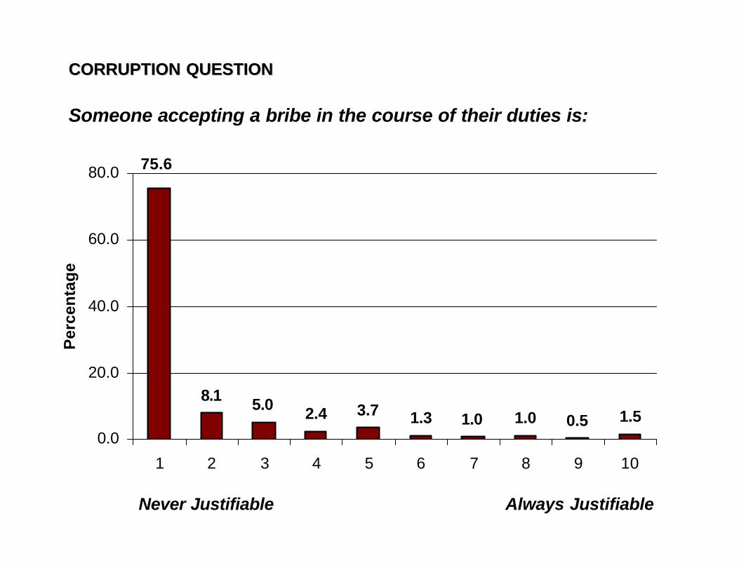
CORRUPTION QUESTIONCORRUPTION QUESTION
Someone accepting a bribe in the course of their duties is:
8.1 5.0 2.4 3.7 1.3 1.0 1.0 0.5 1.5
75.6
0.0
20.0
40.0
60.0
80.0
1 2 3 4 5 6 7 8 9 10
Per
cen
tag
e
Never Justifiable Always Justifiable
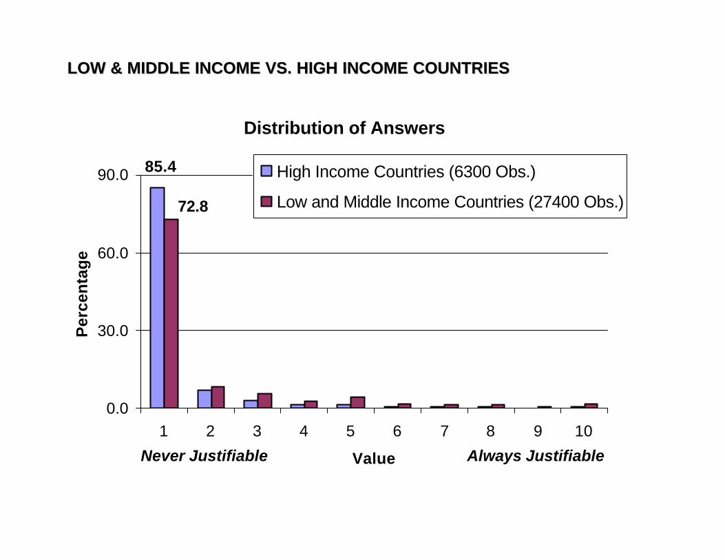
LOW & MIDDLE INCOME VS. HIGH INCOME COUNTRIESLOW & MIDDLE INCOME VS. HIGH INCOME COUNTRIES
Distribution of Answers
85.4
72.8
0.0
30.0
60.0
90.0
1 2 3 4 5 6 7 8 9 10
Value
Per
cen
tag
e
High Income Countries (6300 Obs.)
Low and Middle Income Countries (27400 Obs.)
Never Justifiable Always Justifiable
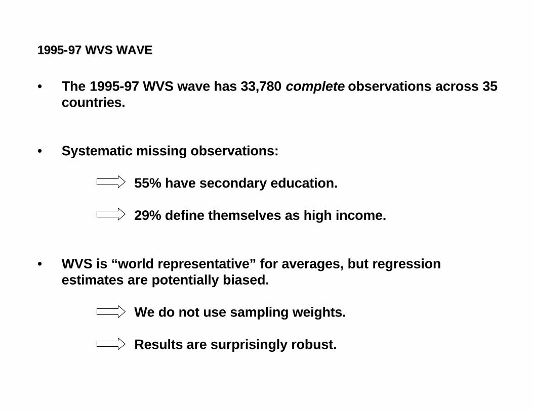
19951995--97 WVS WAVE97 WVS WAVE
• The 1995-97 WVS wave has 33,780 complete observations across 35 countries.
• Systematic missing observations:
55% have secondary education.
29% define themselves as high income.
• WVS is “world representative” for averages, but regression estimates are potentially biased.
We do not use sampling weights.
Results are surprisingly robust.
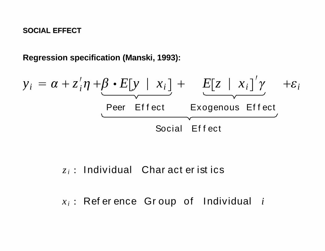
SOCIAL EFFECTSOCIAL EFFECT
Regression specification (Manski, 1993):
z i : Individual Characteristics
x i : Reference Group of Individual i
yi = α + z i′η +
Social Effect
Peer Effect
β ⋅ Ey ∣ xi +
Exogenous Effect
Ez ∣ x i ′γ +i
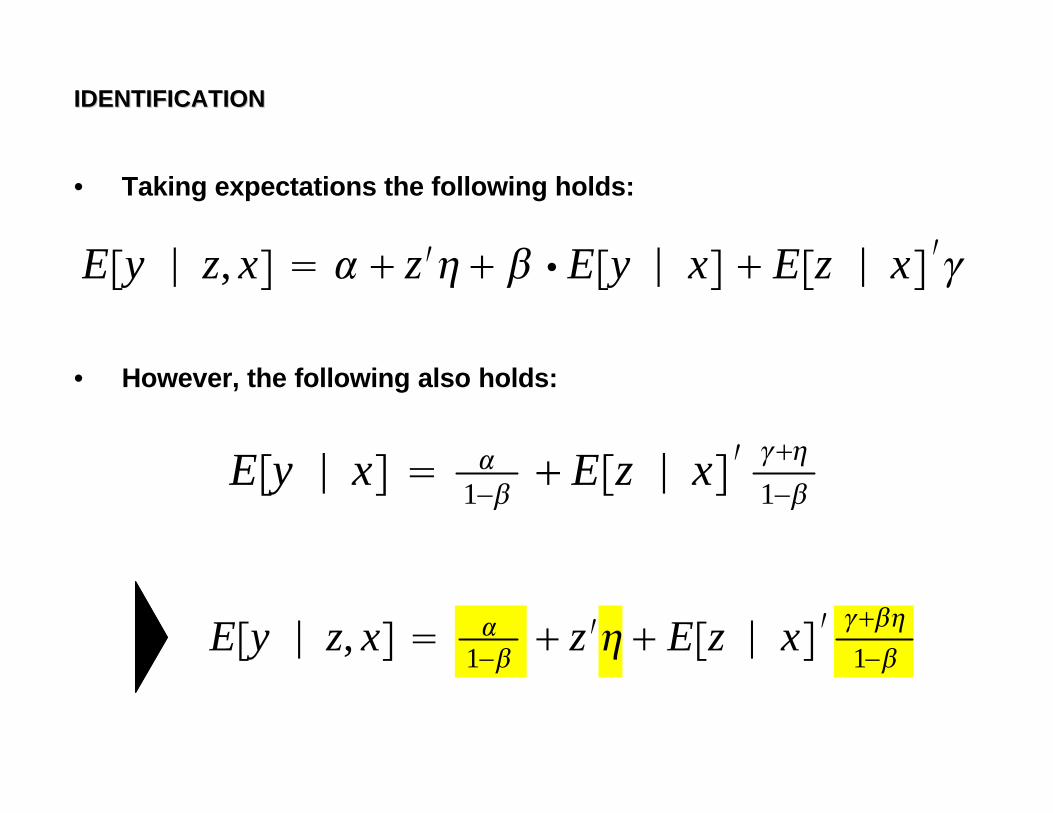
IDENTIFICATIONIDENTIFICATION
• Taking expectations the following holds:
• However, the following also holds:
Ey ∣ z, x = α + z ′η + β ⋅ Ey ∣ x + Ez ∣ x ′γ
Ey ∣ z, x = α1−β + z ′η + Ez ∣ x ′ γ+βη
1−β
Ey ∣ x = α1−β + Ez ∣ x ′ γ+η
1−β
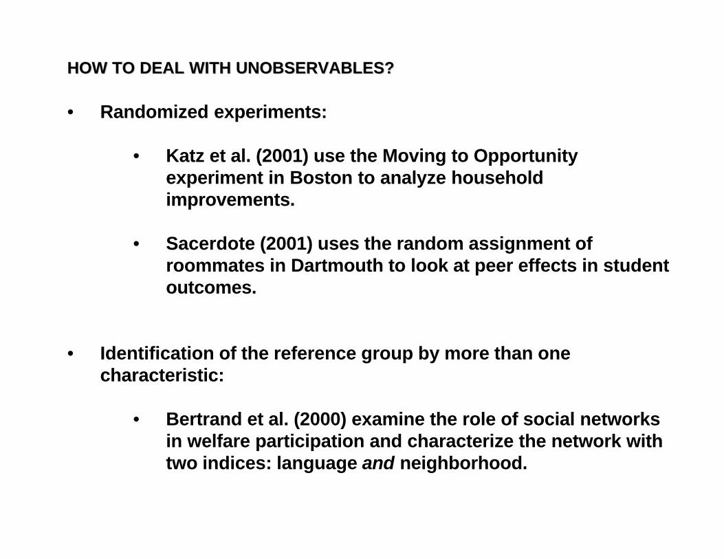
• Randomized experiments:
• Katz et al. (2001) use the Moving to Opportunity experiment in Boston to analyze household improvements.
• Sacerdote (2001) uses the random assignment of roommates in Dartmouth to look at peer effects in student outcomes.
• Identification of the reference group by more than one characteristic:
• Bertrand et al. (2000) examine the role of social networks in welfare participation and characterize the network with two indices: language and neighborhood.
HOW TO DEAL WITH UNOBSERVABLES?HOW TO DEAL WITH UNOBSERVABLES?
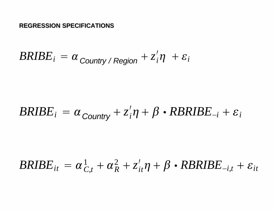
REGRESSION SPECIFICATIONSREGRESSION SPECIFICATIONS
BRIBEi = αCountry / Region + z i′η + i
BRIBEi = αCountry + z i′η + β ⋅ RBRIBE−i + i
BRIBEit = αC,t1 + αR
2 + zit′ η + β ⋅ RBRIBE−i,t + it
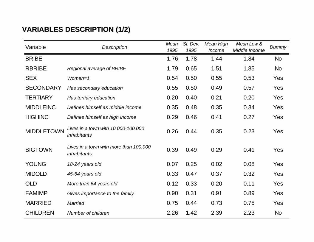
VARIABLES DESCRIPTION (1/2)VARIABLES DESCRIPTION (1/2)
Variable DescriptionMean 1995
St. Dev. 1995
Mean High Income
Mean Low & Middle Income
Dummy
BRIBE 1.76 1.78 1.44 1.84 No
RBRIBE Regional average of BRIBE 1.79 0.65 1.51 1.85 No
SEX Women=1 0.54 0.50 0.55 0.53 Yes
SECONDARY Has secondary education 0.55 0.50 0.49 0.57 Yes
TERTIARY Has tertiary education 0.20 0.40 0.21 0.20 Yes
MIDDLEINC Defines himself as middle income 0.35 0.48 0.35 0.34 Yes
HIGHINC Defines himself as high income 0.29 0.46 0.41 0.27 Yes
MIDDLETOWN Lives in a town with 10.000-100.000 inhabitants
0.26 0.44 0.35 0.23 Yes
BIGTOWN Lives in a town with more than 100.000 inhabitants
0.39 0.49 0.29 0.41 Yes
YOUNG 18-24 years old 0.07 0.25 0.02 0.08 Yes
MIDOLD 45-64 years old 0.33 0.47 0.37 0.32 Yes
OLD More than 64 years old 0.12 0.33 0.20 0.11 Yes
FAMIMP Gives importance to the family 0.90 0.31 0.91 0.89 Yes
MARRIED Married 0.75 0.44 0.73 0.75 Yes
CHILDREN Number of children 2.26 1.42 2.39 2.23 No

VARIABLES DESCRIPTION (2/2)VARIABLES DESCRIPTION (2/2)
Variable DescriptionMean 1995
St. Dev. 1995
Mean High Income
Mean Low & Middle Income Dummy
CHURCH Goes to church at least once a week 0.20 0.40 0.22 0.20 Yes
CATHOLIC Catholic 0.23 0.42 0.36 0.21 Yes
PROTESTANT Protestant 0.09 0.28 0.36 0.02 Yes
ORTHODOX Orthodox 0.24 0.43 0.01 0.30 Yes
MUSLIM Muslim 0.06 0.24 0.00 0.08 Yes
JEW Jew 0.02 0.13 0.01 0.02 Yes
OTHERREL Other religion 0.16 0.37 0.06 0.19 Yes
RIGHT Defines himself politically from the right 0.16 0.36 0.11 0.17 Yes
CENTER Defines himself politically from the center 0.46 0.50 0.60 0.43 Yes
FULLTIME Works fulltime 0.37 0.48 0.37 0.37 Yes
UNEMP Unemployed 0.07 0.26 0.06 0.07 Yes
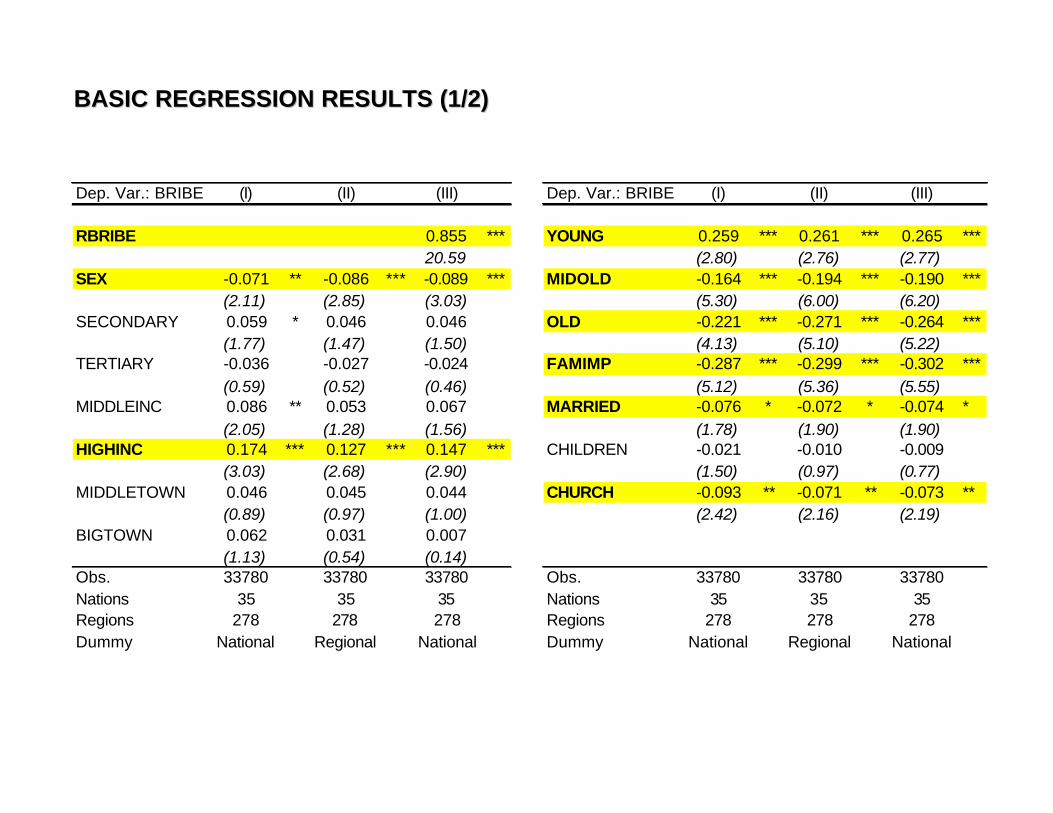
BASIC REGRESSION RESULTS (1/2)BASIC REGRESSION RESULTS (1/2)
Dep. Var.: BRIBE (I) (II) (III)
RBRIBE 0.855 ***20.59
SEX -0.071 ** -0.086 *** -0.089 ***(2.11) (2.85) (3.03)
SECONDARY 0.059 * 0.046 0.046(1.77) (1.47) (1.50)
TERTIARY -0.036 -0.027 -0.024(0.59) (0.52) (0.46)
MIDDLEINC 0.086 ** 0.053 0.067(2.05) (1.28) (1.56)
HIGHINC 0.174 *** 0.127 *** 0.147 ***(3.03) (2.68) (2.90)
MIDDLETOWN 0.046 0.045 0.044(0.89) (0.97) (1.00)
BIGTOWN 0.062 0.031 0.007(1.13) (0.54) (0.14)
Obs. 33780 33780 33780Nations 35 35 35Regions 278 278 278Dummy National Regional National
Dep. Var.: BRIBE (I) (II) (III)
YOUNG 0.259 *** 0.261 *** 0.265 ***(2.80) (2.76) (2.77)
MIDOLD -0.164 *** -0.194 *** -0.190 ***(5.30) (6.00) (6.20)
OLD -0.221 *** -0.271 *** -0.264 ***(4.13) (5.10) (5.22)
FAMIMP -0.287 *** -0.299 *** -0.302 ***(5.12) (5.36) (5.55)
MARRIED -0.076 * -0.072 * -0.074 *(1.78) (1.90) (1.90)
CHILDREN -0.021 -0.010 -0.009(1.50) (0.97) (0.77)
CHURCH -0.093 ** -0.071 ** -0.073 **(2.42) (2.16) (2.19)
Obs. 33780 33780 33780Nations 35 35 35Regions 278 278 278Dummy National Regional National
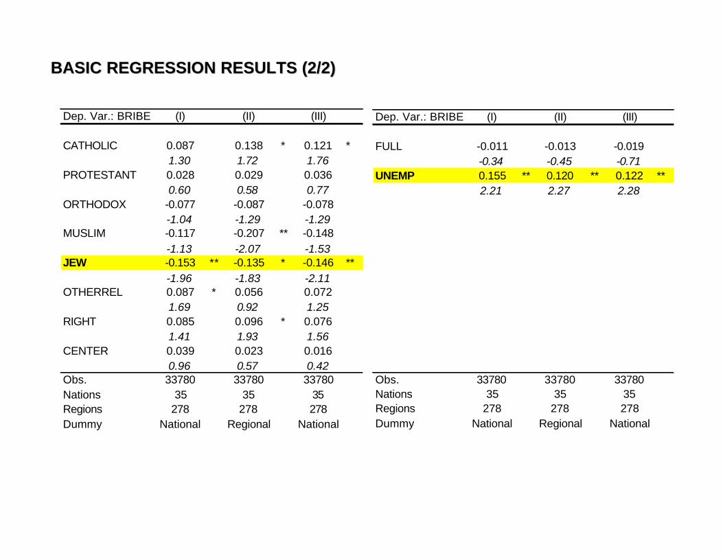
Dep. Var.: BRIBE (I) (II) (III)
CATHOLIC 0.087 0.138 * 0.121 *1.30 1.72 1.76
PROTESTANT 0.028 0.029 0.0360.60 0.58 0.77
ORTHODOX -0.077 -0.087 -0.078-1.04 -1.29 -1.29
MUSLIM -0.117 -0.207 ** -0.148-1.13 -2.07 -1.53
JEW -0.153 ** -0.135 * -0.146 **-1.96 -1.83 -2.11
OTHERREL 0.087 * 0.056 0.0721.69 0.92 1.25
RIGHT 0.085 0.096 * 0.0761.41 1.93 1.56
CENTER 0.039 0.023 0.0160.96 0.57 0.42
Obs. 33780 33780 33780Nations 35 35 35Regions 278 278 278Dummy National Regional National
Dep. Var.: BRIBE (I) (II) (III)
FULL -0.011 -0.013 -0.019-0.34 -0.45 -0.71
UNEMP 0.155 ** 0.120 ** 0.122 **2.21 2.27 2.28
Obs. 33780 33780 33780Nations 35 35 35Regions 278 278 278Dummy National Regional National
BASIC REGRESSION RESULTS (2/2)BASIC REGRESSION RESULTS (2/2)
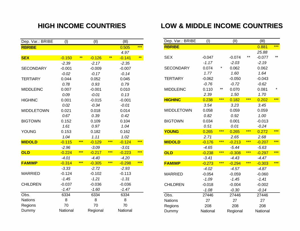
HIGH INCOME COUNTRIESHIGH INCOME COUNTRIES
Dep. Var.: BRIBE (I) (II) (III)RBRIBE 0.505 ***
4.97SEX -0.150 ** -0.126 ** -0.141 **
-2.39 -2.17 -2.35SECONDARY -0.001 -0.009 -0.007
-0.02 -0.17 -0.14TERTIARY 0.044 0.052 0.045
0.78 0.93 0.79MIDDLEINC 0.007 -0.001 0.010
0.09 -0.01 0.13HIGHINC 0.001 -0.015 -0.001
0.02 -0.34 -0.01MIDDLETOWN 0.021 0.018 0.014
0.67 0.39 0.42BIGTOWN 0.152 0.109 0.104
1.61 0.97 1.04YOUNG 0.153 0.182 0.162
1.04 1.11 1.02MIDOLD -0.115 *** -0.129 *** -0.124 ***
-2.96 -3.09 -3.01OLD -0.224 *** -0.217 *** -0.223 ***
-4.01 -4.40 -4.20FAMIMP -0.314 *** -0.305 *** -0.298 ***
-3.33 -2.72 -2.93MARRIED -0.124 -0.102 -0.113
-1.45 -1.21 -1.31CHILDREN -0.037 -0.036 -0.036
-1.47 -1.60 -1.47Obs. 6334 6334 6334Nations 8 8 8Regions 70 70 70Dummy National Regional National
Dep. Var.: BRIBE (I) (II) (III)RBRIBE 0.881 ***
25.88SEX -0.047 -0.074 ** -0.077 **
-1.17 -2.03 -2.19SECONDARY 0.074 * 0.062 0.062
1.77 1.60 1.64TERTIARY -0.062 -0.050 -0.043
-0.76 -0.72 -0.62MIDDLEINC 0.110 ** 0.070 0.081 *
2.39 1.50 1.70HIGHINC 0.238 *** 0.182 *** 0.202 ***
3.54 3.23 3.45MIDDLETOWN 0.058 0.059 0.059
0.82 0.92 1.00BIGTOWN 0.034 0.001 -0.013
0.51 0.01 -0.24YOUNG 0.265 *** 0.265 *** 0.272 ***
2.71 2.65 2.68MIDOLD -0.176 *** -0.213 *** -0.207 ***
-4.65 -5.44 -5.63OLD -0.238 *** -0.308 *** -0.297 ***
-3.41 -4.43 -4.47FAMIMP -0.273 *** -0.294 *** -0.303 ***
-4.02 -4.57 -4.87MARRIED -0.054 -0.059 -0.060
-1.09 -1.45 -1.41CHILDREN -0.018 -0.004 -0.002
-1.08 -0.30 -0.14Obs. 27446 27446 27446Nations 27 27 27Regions 208 208 208Dummy National Regional National
LOW & MIDDLE INCOME COUNTRIESLOW & MIDDLE INCOME COUNTRIES
HIGH INCOME COUNTRIESHIGH INCOME COUNTRIES
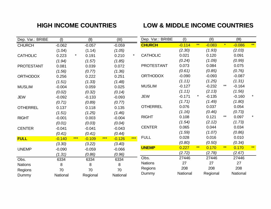
Dep. Var.: BRIBE (I) (II) (III)CHURCH -0.062 -0.057 -0.059
(1.04) (1.14) (1.05)CATHOLIC 0.223 * 0.191 0.210 *
(1.94) (1.57) (1.85)PROTESTANT 0.081 0.039 0.072
(1.56) (0.77) (1.36)ORTHODOX 0.256 0.222 0.251
(1.51) (1.33) (1.48)MUSLIM -0.004 0.059 0.025
(0.02) (0.32) (0.14)JEW -0.092 -0.133 -0.093
(0.71) (0.89) (0.77)OTHERREL 0.137 0.118 0.135
(1.51) (1.25) (1.46)RIGHT -0.001 0.003 -0.004
(0.01) (0.03) (0.04)CENTER -0.041 -0.041 -0.043
(0.41) (0.41) (0.44)FULL -0.140 *** -0.109 *** -0.126 ***
(3.30) (3.22) (3.40)UNEMP -0.090 -0.059 -0.066
(1.31) (0.86) (0.96)Obs. 6334 6334 6334Nations 8 8 8Regions 70 70 70Dummy National Regional National
Dep. Var.: BRIBE (I) (II) (III)CHURCH -0.114 ** -0.083 * -0.086 **
(2.30) (1.93) (2.03)CATHOLIC 0.021 0.120 0.091
(0.24) (1.09) (0.99)PROTESTANT 0.073 0.084 0.075
(0.61) (0.85) (0.76)ORTHODOX -0.090 -0.093 -0.087
(1.11) (1.25) (1.31)MUSLIM -0.127 -0.232 ** -0.164
(1.11) (2.13) (1.56)JEW -0.171 * -0.135 -0.160 *
(1.71) (1.49) (1.80)OTHERREL 0.076 0.037 0.054
(1.16) (0.46) (0.73)RIGHT 0.108 0.121 ** 0.097 *
(1.54) (2.12) (1.73)CENTER 0.065 0.044 0.034
(1.59) (1.07) (0.86)FULL 0.028 0.016 0.010
(0.80) (0.50) (0.34)UNEMP 0.227 ** 0.170 ** 0.170 **
(2.72) (2.78) (2.67)Obs. 27446 27446 27446Nations 27 27 27Regions 208 208 208Dummy National Regional National
LOW & MIDDLE INCOME COUNTRIESLOW & MIDDLE INCOME COUNTRIES
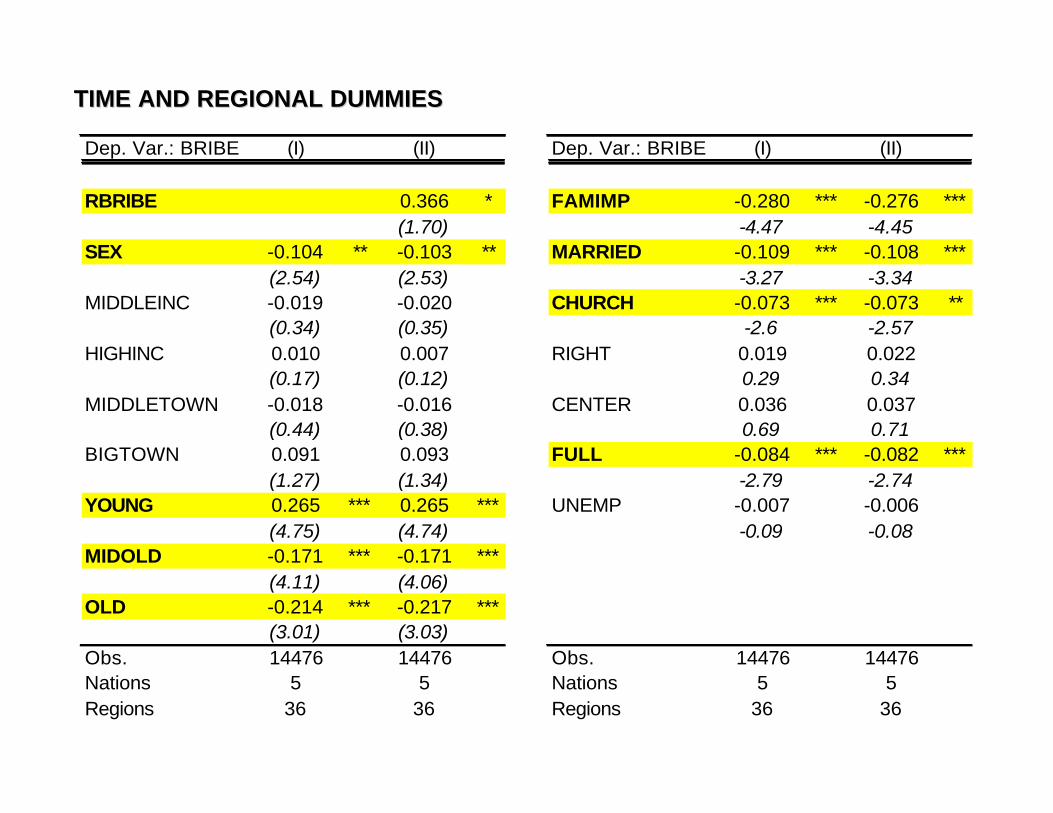
Dep. Var.: BRIBE (I) (II)
RBRIBE 0.366 *(1.70)
SEX -0.104 ** -0.103 **(2.54) (2.53)
MIDDLEINC -0.019 -0.020(0.34) (0.35)
HIGHINC 0.010 0.007(0.17) (0.12)
MIDDLETOWN -0.018 -0.016(0.44) (0.38)
BIGTOWN 0.091 0.093(1.27) (1.34)
YOUNG 0.265 *** 0.265 ***(4.75) (4.74)
MIDOLD -0.171 *** -0.171 ***(4.11) (4.06)
OLD -0.214 *** -0.217 ***(3.01) (3.03)
Obs. 14476 14476Nations 5 5Regions 36 36
TIME AND REGIONAL DUMMIESTIME AND REGIONAL DUMMIES
Dep. Var.: BRIBE (I) (II)
FAMIMP -0.280 *** -0.276 ***-4.47 -4.45
MARRIED -0.109 *** -0.108 ***-3.27 -3.34
CHURCH -0.073 *** -0.073 **-2.6 -2.57
RIGHT 0.019 0.0220.29 0.34
CENTER 0.036 0.0370.69 0.71
FULL -0.084 *** -0.082 ***-2.79 -2.74
UNEMP -0.007 -0.006-0.09 -0.08
Obs. 14476 14476Nations 5 5Regions 36 36
CONCLUSIONSCONCLUSIONS
• Women, employed, less wealthy, and older individuals claim to be more averse to corruption.
• The social environment has a strong influence on the individual attitudes towards corruption – coordinated actions on different fronts are needed to eradicate corruption.
• Although in our analysis we look at the perception of corruption, some results (i.e., women tend to be less corrupt) are consistent with previous studies.