indian statistical institute - northwestern universityusers.iems.northwestern.edu/~ajit/papers/6)...

Indian Statistical Institute

Incomplete Block Designs for Comparing Treatments with a Control (II): Optimal Designs forOne-Sided Comparisons When p = 2(1)6, k = 2 and p = 3, k = 3Author(s): Robert E. Bechhofer and Ajit C. TamhaneSource: Sankhyā: The Indian Journal of Statistics, Series B, Vol. 45, No. 2 (Aug., 1983), pp.193-224Published by: Indian Statistical InstituteStable URL: http://www.jstor.org/stable/25052289Accessed: 22/10/2010 10:05

Your use of the JSTOR archive indicates your acceptance of JSTOR's Terms and Conditions of Use, available athttp://www.jstor.org/page/info/about/policies/terms.jsp. JSTOR's Terms and Conditions of Use provides, in part, that unlessyou have obtained prior permission, you may not download an entire issue of a journal or multiple copies of articles, and youmay use content in the JSTOR archive only for your personal, non-commercial use.

Please contact the publisher regarding any further use of this work. Publisher contact information may be obtained athttp://www.jstor.org/action/showPublisher?publisherCode=indstatinst.

Each copy of any part of a JSTOR transmission must contain the same copyright notice that appears on the screen or printedpage of such transmission.

JSTOR is a not-for-profit service that helps scholars, researchers, and students discover, use, and build upon a wide range ofcontent in a trusted digital archive. We use information technology and tools to increase productivity and facilitate new formsof scholarship. For more information about JSTOR, please contact [email protected].

Indian Statistical Institute is collaborating with JSTOR to digitize, preserve and extend access to Sankhy: TheIndian Journal of Statistics, Series B.

http://www.jstor.org

http://www.jstor.org/action/showPublisher?publisherCode=indstatinst

http://www.jstor.org/stable/25052289?origin=JSTOR-pdf

http://www.jstor.org/page/info/about/policies/terms.jsp

http://www.jstor.org/action/showPublisher?publisherCode=indstatinst

Sankhy? : The Indian Journal of Statistics 1983, Volume 45, Series B, Pt. 2, pp. 193-224.

INCOMPLETE BLOCK DESIGNS FOR COMPARING TREATMENTS WITH A CONTROL (II):

OPTIMAL DESIGNS FOR ONE-SIDED

COMPARISONS WHEN p = 2(1)6,

k = 2 AND p = 3, k = 3

% ROBERT E. BECHHOFER

Cornell University, Ithaca, New York 14853

and

AJIT C. TAMHANE

Northwestern University, Evanston, IVKnois 60201

SUMMARY. In this article we continue the study of balanced treatment incomplete block (BTIB) designs initiated in Bechhofer and Tamhane (1981). These designs are appropriate for comparing simultaneously p > 2 test treatments with a control treatment in blocks of com

mon size k < p+l. The general class of BTIB designs was characterized in that first article.

In the present article we study in detail the particular cases p > 2, k = 2 and p = 3. k = 3.

These cases share a special property, namely that there are only two so-called generator designs in the minimal complete set. This fact enables us to give for these cases a simple characteriza

tion of admissible designs which are the only contenders for optimal designs.

We have computed tables of discrete optimal designs for joint one-sided comparisons for

the cases p =

2(1)6, k = 2 and p = 3, k = 3. The special property possessed by these cases

also enables us to develop a simple continuous approximation to the discrete optimal designs.

Using this approximation we have computed analogous tables of continuous optimal designs ;

these tables can be used when large 6-values are required. The theory underlying the approxi mation is developed, and its goodness is assessed.

1. Introduction

In Bechhofer and Tamhane (1981) (referred to hereinafter as B-T) we

initiated the study of balanced treatment incomplete block (BTIB) designs which are appropriate for comparing simultaneously p > 2 test treatments

with a control treatment in blocks of common size k <p+1. This general class of designs was characterized in B-T. In the present article we obtain

optimal designs within this class for p = 2(1)6, k = 2 and p

= 3, k ? 3.

The cases p > 2, k = 2 and p = 3, k = 3 share a special property, namely

that there are exactly two so-called generator designs in the minimal complete set for each of the (p, &)-values. (See Section 2.2 for definitions of the various

technical terms used in this section.) This feet enables us to give a simple characterization of admissible designs for these cases.

194 ROBERT E. BECHHOFER AND AJIT C. TAMHANE

When the minimal complete set consists of only two generator designs, it is possible to develop a simple continuous approximation to the discrete

optimal designs. The problem of obtaining the continuous optimal designs is easy to solve on a computer. Also, use of the approximation substantially reduces the number of designs to be tabulated. In the present article we

give discrete as well as continuous optimal designs for one-sided comparisons with a control. More detailed tables of discrete optimal designs for the

(p, &)-values considered in the present article as well as for many additional

ones of practical interest are given in Bechhofer and Tamhane (1983) both for

one-sided and for two-sided comparisons.

In order to make the present article self-contained we state below the

key definitions and results from B-T. We shall use the following notation

(also used in B-T) : Let the treatments be indexed by 0, 1, ...,p with 0

denoting the control treatment and \,2, ...,p denoting the test treatments.

The N = Jcb experimental units can be arranged in b blocks each of common

size Jc. If treatment i is assigned to the A-th plot of the j-th block

(0 < i < p, 1 < h < Je, 1 < j < b), let Yijk denote the corresponding random

variable; we assume the usual additive linear model (no treatment X block

interaction) Y m =P+*i+?j+etjh ... (1.1)

p b

with ? at = T? ?j ?0; the e^? are assumed to be i.i.d. iV(0, <r2) random

variables, and cr2 is assumed to be known. It is desired to make joint interval

estimates (employing one-sided or two-sided intervals) of the p differences

a0?ol% based on their best linear unbiased estimators (BLUE's) ?r0?a.

(1 < i < p).

In Section 3.1 of B-T we proposed a class of incomplete block designs which are balanced with respect to the test treatments in the following sense :

var{?0?&i} =rV2 (1 (ix ̂ i2; 1 < iv

i2 < _p); the parameters r and p depend on the design employed. We refer

to designs with this property as BTIB designs. (We have recently learned

that Pearce (1960) had proposed designs with this same property; he called

them designs with "supplemented balance.") Conditions that a design must

satisfy in order that it be BTIB were given in Theorem 3.1 of B-T. This

theorem states that if {r?j} is the incidence matrix of the design, r^ being the

total number of times the i-th treatment appears in the j-th block, and if b

?. . = 2 r. /. , which is the total number of times that the i^th treatment *1*2 ^

lU Hi 1

appears with the ?2-th treatment in the same block over the whole design

BALANCED TREATMENT INCOMPLETE BLOCK DESIGNS 195

(h =?hl 0 < iv i2 < p), then the necessary and sufficient conditions for a

design to be BTIB are that

^01 =^02 =

=^op =

^o (say)

Aia =

Au = ... =

?p?lf p = Ax (say)

for some A0, Ax > 0. In Section 4 of B-T we restricted consideration to BTIB

designs, and showed how to use such designs for experiments leading to joint one-sided (or two-sided) confidence interval estimates of the a0?a? (1 < i < p)

when a2 is known (or unknown).

The specific multiple comparisons with a control (MCC) problem with

which we are concerned in the present article is that of obtaining joint one

sided confidence intervals of the form

K-a, > Ao-?t-a (1 < % < p)} ... (1.2)

for given values of (p, k) when or2 is known, and a > 0 is a specified "allowance"

associated with the common "width" of the confidence intervals. For this

problem we seek an optimal design in the class of all admissible BTIB designs, an optimal design being one which minimizes b, the total number of blocks

required to achieve a specified confidence coefficient 1?a associated with (1.2).

2. Preliminaries

2.1. Expressions for joint confidence interval estimates. For ease of

reference we record here the expressions derived in B-T for the estimators

?o?&i (1 ^ * ̂ P)> an(i their variances and correlations. Let T4 denote

the sum of all observations obtained with the i-th treatment (0 ̂ i < p),

and let Bj denote the sum of all observations in the j-th block (1 < j < 6).

Define B\ = 2 r^Bj and let Qx = kTt-B* (0 ) ... (2.2)

. _ ?(Ao+AJ M*o+p*i)

' (2.3)

and

p = oarrf?,??^, ?^-?^}

= j^rj- (h ?> H\ 1 < *i> ?a < P)- (2-4)

The probability associated with (1.2) is given by

P{a0-oci > ?0?fa?a (1 (x); ... (2.5)

here <_>( ) denotes the standard normal c.d.f. and for notational simplicity we

have let

f=^=?}> ... (2.6)

\{K+pK) and _

?=aVJcbl<r, ... (2.7)

both of which are pure numbers.

2.2. Generator designs, admissible designs, and minimal complete set of

generator designs. We begin with the concept of a generator design. For

given (p, k) a generator design is a BTIB design such that no proper subset

of its blocks forms a BTIB design and none of its blocks contains only one

of the p-\-l treatments.

Next we define an admissible design. If for given (p, h) we have two

BTIB designs D and D', with parameters (b, A?, ?^ r, p) and (&', ?0, ?[, r', p'),

respectively, with b < b', and if for every a and er, D yields a confidence co

efficient no smaller than (resp., larger than) that yielded by D' when b <b'

(resp., b = b') then we say that D' is inadmissible with respect to (w.r.t.) D.

In Theorem 5.1 of B-T the following condition was shown to be necessary and

sufficient for D' to be inadmissible w.r.t. D : b ^ b', r ^ r', and p > p' with

at least one inequality strict. If a design is not inadmissible then it is said

to be admissible. If b = b', r = r', p =pf then we say that D and D' are

equivalent since they yield the same confidence coefficient (2.5) for all values

of a and or. A minimal complete set of generator designs is the smallest set

of generator designs D = {_D1? D2, ..., Dn} from which all admissible designs

can be constructed for given (p, 1c) (except possibly any equivalent designs).

A method for obtaining the minimal complete set for any given (p, Jc) is des

cribed in Section 5 of B-T.

2.3. Optimal designs. For given (p, k), let D ? {Dv D2, ..., Dn} denote

the minimal complete set of generator designs. Let A^>, \[l) be the design

parameters associated with Dh and let b\ be the number of blocks required

by Di (1 0 replications of D?, (represented as D = JJ /?A) has the design para i = l

BALANCED TREATMENT INCOMPLETE BLOCK DESIGNS 197 n n n

meters A0 = S fiXf and Ax = S fiXf and requires b = S ffa blocks.

We shall consider only implementahle D, i.e., those for which A0 > 0. It

should be noted that for given D the design D is completely determined by its frequency vector f ={fv ...,/J.

As mentioned at the end of Section 1, an optimal design minimizes b in

the class of all admissible designs which for (1.2) achieve at least a specified confidence coefficient 1?a. The problem of finding an optimal design is

solved numerically in two steps which are described below.

In the first step b is fixed and for given (p, k), D, and specified a/or, / is n

chosen to maximize (2.5) among all admissible / satisfying 2 /?6? =6, n

2 /?^(o > ? and fi > 0 (1 < i < n). In this setup the integral expression <=i

(2.5) for the confidence coefficient can be regarded as a function of / for given

(p, k), D, b and for specified ? =

aVkblcr. We therefore denote (2.5) by

g(f\D; p,k,b;?) =g (say). Let g denote the maximum value of g for that A.

b and let / denote the BTIB design that yields g. This procedure of finding

/ and its associated g is repeated for all values of b for which admissible

designs exist. Thus this first step generates a table of / and g for different

b and the specified a\cr. In the second step, the specified 1?a and a/cr are fixed and 6 is varied.

Then by referring to the table of (/, g), the / with the smallest b (say, b) for

which g > 1?a is determined. This procedure of finding an optimal design is illustrated in Section 4 for the special case p

= 2, k = 2.

3. Minimal complete sets of generator designs and admissible

DESIGNS FOR p > 2, k = 2, AND p = 3, k = 3

3.1. Minimal complete sets of generator designs for p ^ 2, k =2 and

p = 3, k = 3. For p > 2, i = 2 and #

= 3, & = 3 the minimal complete sets

of generator designs always have cardinality two. For p > 2, k = 2 this is

clear since the only two generator designs possible are

rOO 0-^ f11 i>?x 1 ?>0=<{

... ?>, D, =

^ ...

J.. ... (3.1) {l 2 pj 12 3 p J

For Z>0 of (3.1) we have

&o=2>, A<o0)=l, A<?>=0, ... (3.2)

198 ROBERT E. BECHHOFER AND AJTT C. TAMHANE

Z>,=

and for Dx of (3.1) we have

^ _-**=!->, A<?=0, A<1>=1. ... (3.3)

Thus for any BTIB design D =/0D0 (J AA for p > 2, fc = 2 we have

6=_>{/o+^i^-7i}. \=U A. ?A. ... (3.4)

For j) = 3, k = 3 it is shown in Notz and Tamhane (1983) that

0 0 0-| ?

1 ^

1 1 2 L Dt =<> 2 y ... (8.5)

L2 3 3j L 3 J

constitutes the minimal complete set. (The problem of constructing the

minimal complete sets of generator designs for p > 3, k = 3 is nontrivial;

this problem is addressed in the Notz-Tamhane article where the minimal

complete sets are given for p =

3(1)10, k = 3.) For D0 of (3.5) we have

60=3, A<8>=2, A<?>:=1, ... (3.6)

and for D1 of (3.5) we have

61=1, A<J)=0, ?<?>=1. ... (3.7)

Thus for any BTIB design /0_D0 (J/A for p = 3, /i = 3 we have

6=3/0+^, A0=2/0, A1=/0+/1. ... (3.8)

In the sequel we will only consider the BTIB designs obtained for given (_p, k)

from the generator designs in the minimal complete set for that (p, k).

3.2. Characterization of admissible designs for _p > 2, k = 2 and p = 3,

k = 3. To characterize the admissible designs we first introduce the concept

of a b-admissible design : For given (p, k), a BTIB design D requiring b

blocks is said to be b-inadmissible if it is inadmissible w.r.t. another BTIB

design also requiring b blocks. If a design is not 6-inadmissible then it is

said to be 6-admissible. (See Table 4.1 A for examples of 6-inadmissible

designs.) A 6-admissible design sometimes can be inadmissible w.r.t. a design

with a smaller 6, but a 6-inadmissible design is always inadmissible.

The importance of the 6-admissibility concept lies in the fact that for

p ^ 2, k = 2 almost all 6-admissible designs are admissible with only a very

small number of exceptions while for p = 3, k = 3 all 6-admissible designs

are admissible. This fact suggests that it usually is sufficient to restrict

consideration to 6-admissible designs for the purpose of obtaining optimal

designs.

We now recall the necessary and sufficient condition, given in Section 2.2,

for a design to be inadmissible w.r.t. another design. For 6-inadmissibility

that condition can be stated simply as follows : For given (p, k) let D and

Df be two BTIB designs with b = 6', and parameters (r?, p) and (?/', p'), res

pectively. The design D' is b-inadmissible w.r.t. the design D iff r? < rf

and p?*pf with at least one inequality strict. If a- design is not 6-inadmissible

then it is b-admissible.

We note that this simpler condition compares designs in terms of their

^-values rather than their T-values. This is permissible because from (2.6) we see that r\\r\'

? t?t' when 6=6'.

Using this condition, 6-admissible designs are characterized in the follow

ing theorem.

Theorem 3.1 : Let (p, k) and the associated minimal complete set of genera

tor designs {D0, Dt} be given where D0 contains both the control and the test

treatments while Dx contains only the test treatments. Let (6?, A^, A^) be the

parameters associated with D? (i = 0, 1) where A^>

= 0. For fixed 6 consider all

designs D =/o^o U/i^i w^1 /0&0+/A == & Letffi denote the upper bound on

/0. Then one of the following two cases obtain depending on the value of

Case 1 : If ? > 0 then there exists an integer fl > 2 which is the smallest

value of/0 satisfying ?/2(/0) > V2(fo?d); here d is the smallest positive integer such that bx divides (60d). If /* < f]f then all designs D with /0 > /J are

b-admissible.

Case 2 : If ? ^ 0 then all designs D are 6-admissible.

Corollary : For p > 2, k = 2, Case 1 holds while for p = 3, fe = 3, Case 2

holds.

The proof of the theorem is given in Appendix 1. If Case 1 holds, then

6 must be sufficiently large in order that /? < /??. As 6 increases the number of designs eliminated as being 6-inadmissible increases.

The corollary follows directly for p > 2, k = 2 by substituting (3.2) and (3.3) in (3.9) and verifying that ? =p{p?l)?2 > 0 and for p = 3, k = 3

by substituting (3.6) and (3.7) in (3.9) and verifying that ? = ? 3 < 0.

B2-7

200 ROBERT E. BECHHOFER AND AJlT C. TAMHANE

The proof of Theorem 3.1 uses a technique (discussed in detail in Section 5)

which regards y ==60/0/6 as a continuous variable taking values in (0, 1]. If y* denotes the minimizing value of if (regarded as a function of y) then

for Case 1, y* is given by solving the equation drf\dy = 0 (see (A. 4) in Appen

dix 1 for an expression for d?/2/dy); for Case 2, y* = 1. The quantity y* is

the maximum permissible proportion of blocks that can be allocated to D0 in a design D with the latter being 6-admissible (assuming that a BTIB design exists for every y e (0, 1]). Therefore a characterization of 6-inadmissibility in the continuous case can be given as follows : For given (p, k), {D0, D?} and 6, a design f0D0 {Jf1D1 is 6-inadmissible iff

/o>-T"-

' - (3-10)

?0

This characterization of 6-inadmissibility in the continuous case can be

expected to approximate closely the exact characterization in the discrete

case (cf. Theorem 3.1) for sufficiently large 6. However, for small or moderate

6 the former characterization may classify a design as 6-inadmissible when,

in fact, it is not. This can happen because of one of two reasons : (i) For

given 6 there may exist only one BTIB design in which case it is automatically

6-admissible although it may satisfy (3.10). (ii) The critical number fl

(defined in Theorem 3.1) which provides an exact characterization of 6-admis

sibility for the discrete case is always greater than 6y*/60. Therefore, a design

/o^oU/A w^tli by*?b0 </0 </o Is 6-admissible although it satisfies (3.10).

For p > 2, k = 2, the value of y* is given by

--1?1 JjZL?l] for_?> 2,p^3, k =2

y=\ (p-QlVp+l - P P ... (3.11)

L 3/4 for p = 3, k = 2.

The corresponding exact values o?fl are given by (4.2).

We now state

Theorem 3.2: For given (p,k) and {D0, DJ let D = foD0{jf1D1 and

D' =/??0[J/i?i be two BTIB designs where {D0, D-} is given by (3.1) for _p > 2, k = 2 and by (3.5) for p = 3, k = 3, respectively. Let (6, r, p) and

(&', t', p') with 6 < V denote the parameters associated with D and U, respectively.

(i) For _p > 2, k =2, if f0 < 6y*/60 and f? < b'y*lb'0 where y* is given

by (3.11), then D' cannot be inadmissible w.r.t. D.

(ii) For p =3, k =3, D' cannot be inadmissible w.r.t. D.

Proof: See Appendix 1.

For p =3, k =3, the corollary of Theorem 3.1 states that all BTIB

designs are 6-admissible; this together with part (ii) of Theorem 3.2 implies that all BTIB designs for p

= 3, k = 3 are admissible. Also note that

part (i) of Theorem 3.2 does not assert that if a design is 6-admissible then it

is admissible; this statement, unfortunately, is not always true. By an

exhaustive enumerative computer search for the cases p =

2(1)6, k = 2 with

6 < 200 a total of only four 6-admissible designs that are inadmissible were

found. These designs are listed below along with the corresponding dominat

ing design with smaller 6 :

(i) p = 4, k = 2 : The design 4D0 which is 6-admissible for 6 =16

and has (r2 = 0-5000, p

= 0-0000) is inadmissible w.r.t. the design 2D0 \J Dt

with 6 = 14 and (r2 = 0-5000, p

= 0-3333).

(ii) p = 6, k = 2 : (a) The design 5D0 which is 6-admissible for 6 = 30

and has (r2 = 0-4000, p

= 0-0000) is inadmissible w.r.t. the design 2D0 (J Dx

with 6 =27 and (r2 =0-3750, p =0-3333).

(b) The design 9Z>0 (J Dx which is 6-admissible for 6 =69 and has

(r2 =0-1481, /) =0-1000) is inadmissible w.r.t. the design 6D0 (J 2BX with

6 =66 and (r2 =0-1481, p =0-2500).

(c) The design 10D0 (J Z)a which is 6-admissible for 6 =75 and has

(r2 =0-1375, p =0-0909) is inadmissible w.r.t. the design 7D0 (J 2D1 with

6 =72 and (r2 =0-1353, p =0-2222).

It can be expected that for large 6 such exceptions will not arise. There

fore, for convenience, we restrict consideration to 6-admissible designs, and

we search for optimal designs among them (recognizing the fact that a very

small number of 6-admissible designs will yield confidence coefficients lower

than those yielded by some designs with smaller 6-values, and hence the former

cannot be optimal).

4. Discrete optimal designs

4.1. Results for # > 2, k = 2. For p > 2, k = 2, any BTIB design

D can be written ^fQD0[JflD1 where {D0, Dx} is given by (3.1) with/0 > 1,

/x ^ 0. The values of 6, A0 and Ax for D are given by (3.4) which when sub

stituted in (2.6) and (2.4) yield

vHn ?b{2b+p(p-3)f0} ( V{f?]-- pf0{2b-(p+l)f0}

' " (4-la)

and

P(fo) = 2(6-i>/o)

(4.1b) 2b+p(p-3)f0

'

The corollary to Theorem 3.1 states that Case 1 holds for all# > 2. In what

follows, we fix 6 in order to determine the 6-admissible designs. The critical

number /o referred to in Theorem 3.1 is the smallest /0 satisfying equation

(3.4) for given 6, and for which y2(f0) > V2(fo~d); here d = p?\ if p is even,

and d = (#?1)/2 if ^? is odd. We thus obtain

/?= J

. , r 2&+i /&* 11

intl-ir Vi + i-J

-m

^-^V

for j) = 2

for # = 3

4(j)-l)a# d2 for# >4

(4.2a)

(4.2b)

(4.2c)

where int[z] denotes the smallest integer ^ z.

We now consider in detail the special case p =

2, k = 2 in order to show

how we obtain optimal designs using the two-step method described at the

end of Section 2.

For p = 2, & = 2, all designs D=fQD0[Jf1Dl are generated from

{D0, DJ of (3.1) for arbitrary 6 = 2/0+./i (6 = 2, 3, ...) where 1 </0 < 6/2,

TABLE 4.1A. ENUMERATION OF DESIGNS1 FOR p = 2, k

r0 0* 2 AND 6 = 2(1)10

?>n

c > *-o

i 2 *3 1 2 3

8.00

8.00

9.60 8.00

11.43 7.50

3.33 8.00 8.00

15.27 8.75 7.47

0.000

0.500

0.667 0.000

0.750 0.333

0.800 0.500 0.000

0.833 0.600 0.250

10 10 10 10 10

1 2 3

*4

1 2 3 4

1 2 3 4

*5

17.23 9.60 7.62 8.00

19.20 10.50

8.00 7.50

21.18 11.43

8.48 7.50 8.00

0.857 0.667 0.400 0.000

0.875 0.714 0.500 0.200

0.889 0.750 0.571 0.333 0.000

1 The designs marked with an asterisk ( *

) are 6-inadmissible.

0 < A < 6?2 for 6 even, and 1 < /0 < (6-l)/2, 1 < ft < 6-2 for 6 odd.

Equation (4.2a) gives f? while fj[ = 6/2 or (6?1)/2 according as 6 is even or

odd; all 6-inadmissible /0 then satisfy /? </0</o- Thus for 6 < 5, all

(/o>/i) are 6-admissible; for 6 = 6, (/0,/x) =

(3, 0) is 6-inadmissible; for

b == 20, (/o,A) =(9, 2) and (10,0) are 6-inadmissible, etc. In Table 4.1 A

we have enumerated all designs for 6 = 2(1)10, and have given the associated

r?2 and />; the 6-inadmissible designs are noted.

Conceptually, one then proceeds as follows : We are given (p, k),

{D0, Dj}, and ajcr is specified. We fix 6 and list all 6-admissible designs for

that 6. Thus from Table 4.1 A we see that for p =

2, k = 2, there are four

6-admissible designs for 6 = 10. For each 6-admissible design we then

calculate g as a function of a/o- and find the design which is associated with g,

the maximum value of g for that 6 and ajtr. Table 4.1B shows for 6 = 10

the designs maximizing g and their associated ^-values for a?cr =

0-5(0-l)l?0.

(For ajcr sufficiently small the design (/0,/i) = (1, 8) is optimal while for aja

sufficiently large the design (/0,/i) =

(4, 2) is optimal; this an example of the

standard phenomenon referred to in the proof of Theorem 5.1 of B-T.) Finally, such tables can be prepared for arbitrary 6^2.

TABLE 4.1B. OPTIMAL DESIGN AND ASSOCIATED CONFIDENCE COEFFICIENT AS A FUNCTION OF a/a FOR p = 2, h = 2 WHEN b = 10

ajcr 0.5 0.6 0.7 0.8 0.9 1.0

/o 3 3 4 4 4 4

A 4 4 2 2 2 2

g 0.6673 0.7248 0.7806 0.8303 0.8719 0.9057

If g is strictly increasing in 6 for all values of ajcr then such tables provide

optimal designs with each listed design being optimal for the corresponding

values of a/or. However, this is not the case for all (p, k); e.g., this is not

the case for p = 4, k = 2. For fixed ajcr, if g decreases or stays constant as

6 increases then one must delete the designs having the larger 6-values when

the associated ^-values are no larger than that yielded by a design with a

smaller 6-value. Using this elimination procedure, detailed tables have been

prepared for p =

2(1)6, k = 2 and p =

3(1)6, k = 3 for selected values of

6 and afor; these are given in Bechhofer and Tamhane (1983). In the present

paper we have obtained the optimal designs from such tables for selected

1?a and a\<x. Tables 4.2-4.6 list for p =

2(1)6, respectively, with k = 2

the optimal designs for 1?a = 0-80, 0-90, 0-95, 0-99 and a/cr =

0-2(0-2)2-0.

4.2. Results for p -= 3, k = 3. For p = 3, i = 3 any BTIB design Z>

can be written as /0#0U/iA. where {D0, DJ is given by (3.5) with /0 > 1,

fx > 0. The values of 6, A0, A2 for D are given by (3.8) which when substituted

in (2.6) and (2.4) yield

962 ?) = m=?>

- (4-3a)

and

(*fo) =

?:??. .- (4.3b)

The corollary to Theorem 3.1 states that Case 2 holds for p =

3, k = 3. This

together with Theorem 3.2 shows that all designs D = fQDQ \J fxDx are

admissible for # =

3, & = 3. Table 4.7 lists for # =

3, k = 3 the optimal

designs for 1?a = 0-80, 0-90, 0-95, 0-99 and a/cr

= 0-2(0-2)2-0.

TABLE 4.2 DISCRETE OPTIMAL DESIGNS TO ACHIEVE A SPECIFIED CONFIDENCE

COEFFICIENT (1-a) AS A FUNCTION OF a/a FOR ONE-SIDED

COMPARISONS (THE UPPER ENTRY IN EACH CELL IS /0,

AND THE LOWER ENTRY IS fv)

p **-*M? I)' Ml)

6 = 2/0+/

confidence aja coefficient

(1-a) 0.2 0.4 0.6 0.8 1.0 1.2 1.4 1.6 1.8 2.0

258 64 29 16 10 8 5 4 3 3

0.99 100 26 11 7 5 2 3 2 2 1

144 36 16 9 6 4 3 2 2 2

0.95 63 16 7 4 3 2 2 2 1 0

96 24 11 6 4 3 2 2 2 1

0.90 .49 13. 5 4 2 1 1.1 0 1

51 13 6 3 2 2 11 11

0.80 34 8 4 3 2 11 1 0 0


TABLE 4.3 DISCRETE OPTIMAL DESIGNS TO ACHIEVE A SPECIFIED CONFIDENCE COEFFICIENT (1-a) AS A FUNCTION OF ajo- FOR ONE-SIDED

COMPARISONS (THE UPPER ENTRY IN EACH CELL IS f0, AND THE LOWER ENTRY IS /-)

/0 0 0* f1 1 2, p

= 3, k = 2, D0

= \ },__).___

I

ll. 2 3' 12 3 3>

b = Vo + 3/i

confidence coefficient

(1-a) 0.2 0.4

ajcr

0.6 0.8 1.0 1.2 1.4 1.6 1.8 2.0

0.99

241

84

61

21

27

10

16

5

10

4

0.95

0.90

0.80

141

56

98

44

56

32

36

14

25

11

14

8

16

6

11

5

9

4

6

3

4

2

6

2

4

2

3

1

4

2

3

1

2

1

TABLE 4.4. DISCRETE OPTIMAL DESIGNS TO ACHIEVE A SPECIFIED CONFIDENCE COEFFICIENT (1-a) AS A FUNCTION OF a\v FOR ONE

SIDED COMPARISONS (THE UPPER ENTRY IN EACH CELL IS /0,

AND THE LOWER ENTRY IS /_)

(0 0 0 0. rl 1 p = ?,k=2,DQ =

\ , D1=\ ll 2 3 4J 12 3 I)


(1-a) 0.2 0.4

a/a

0.6 0.8 1.0 1.2 1.4 1.6 1.8 2.0

0.99

226

73

57

18

24

9

14

5

0.95

136

49

33

13

16

5

0.90

97

39

24

10

10

5

0.80

56

30

15

7

2

0


TABLE 4.5. DISCRETE OPTIMAL DESIGNS TO ACHIEVE A SPECIFIED CONFIDENCE COEFFICIENT (1-a) AS A FUNCTION OF aja FOR ONE

SIDED COMPARISONS (THE UPPER ENTRY IN EACH CELL IS/0,

AND THE LOWER ENTRY IS fx) ,00000. fl 11122233 4?

V1234 5? 12 34534545 5) p = 5, k

2 3 4 5J '

6 = 5/0+10/1


d-a)

a/cr

0.2 0.4 0.6 0.8 1.0 1.2 1.4 1.6 1.8 2.0

0.99

0.95

0.90

0.80

213

65

132

44

94

36

58

27

54

16

33

11

24

9

14

7

25

7

15

5

11

4

7

3

14

4

8

3

7

2

4

2

3

1

2

1

1

1

2

0

TABLE 4.6. DISCRETE OPTIMAL DESIGNS TO ACHIEVE A SPECIFIED CONFIDENCE COEFFICIENT (1-a) AS A FUNCTION OF a\v FOR ONE

SIDED COMPARISONS (THE UPPER ENTRY IN EACH CELL IS/0,

AND THE LOWER ENTRY IS %)

f0 0000 0? rl 1111222233344 5^ ,, D1== \ 2 345 6? 12 3456345645656 6J

p = 6, k :

confidence coemcient

(1-a)

0.99

0.95

0.90

0.80

0.2

205

57

129

39

94

32

55

26

0.4

52

14

32

10

24

8

15

6

M r1 L L

?J 12 3 4

S = 6/0+15/;

0.6

24

6

13

5

12

3

6

3

0.8

12

4

7

3

6

2

a?cr

1.0

9

2

1.2

5

2

4

1

3

1

2

1

1.4 1.6

3

1

2

1

1

1

3

0

1.8

2

1

1

1

3

0

2

0

2.0

2

1

3

0

3

0

2

0

JBA?AKCED TREATMENT INCOMPLETE BLOCK DISSIONS 20tf

TABLE 4.7. DISCRETE OPTIMAL DESIGNS TO ACHIEVE A SPECIFIED CONFIDENCE COEFFICIENT (1-a) AS A FUNCTION OF a/o- FOR ONE

SIDED COMPARISONS (THE UPPER ENTRY IN EACH CELL IS/?Y

AND THE LOWER ENTRY IS /_)

i> = 3,fc = 3,D0=- ll 1 2],

A? (21

6 = 3/o +J_

confidence a\& coefficient ?-?

(1-a) 0.2 0.4 0.6 0.8 1.0 1.2 1.4 1.6 .1.8 2.0

164 41 18 10 7 5 3 3 2 2 0.99 0 0 1 10 0 2 0 1 0

98 25 11 6 4 3 2 2 1 1 0.95 2 0 0 10 0 10 1 0

71 18 8 4 3 2 2 11 1 0.90 1 0 0 2 0 0 0 10 0

41 10 5 3 2 11 1 1 1 0.80 8 3 0 0 0 10 0 0 0

5. Continuous optimal designs

5.1. Preliminaries. As in Section 3 we continue to deal with situations

in which the minimal complete set consists of two generator designs D0 and

Dx where D0 contains both the control and th? test treatments while Dx contains

only the test treatments. In Section 4 we noted that, in general (but not

always), the number of competing admissible designs increases with 6 for

fixed (p, k). We have seen that for each (p, k) the optimal design depends on

a/cr; also, the determination of the optimal design requires that the design

maximizing g be found for each (p, k, 6) and a/or combination. This represents a formidable computing and tabulation task. The solutions for many of the

useful combinations are given in Tables 4.2-4.7.

In order to extend the results given in Section 4, and to do so in a compact

form we introduce a method for finding an approximation to the discrete

optimal designs. We shall refer to such designs as continuous optimal designs.

The problem of obtaining the continuous optimal designs is analytically more tractable and computationally easier to solve. Moreover, since its

solution does not depend individually on 6 and a/c but only on these quantities

through ? =

aVkbJcr, the number of solutions that must be tabulated is

drastically reduced. In Section 5.7 we assess how closely the approximate

discrete optimal designs (obtained from the continuous optimal designs)

agree with the exact discrete optimal designs.

B2-8

5.2. Definition of y. For given (p, k) and the associated minimal com

plete set of generator designs {D0, DJ we define for an arbitrary BTIB design D =f0Do?fi?>v the quantity

y~ b -foK+Ah ' (5)

which is the proportion of the total number of blocks allocated to D0. For

large values of 6 we shall treat y e (0, 1] as a nonnegative continuous variable.

Then regarding <r?2 and p of (2.6) and(2.4) (see also (A.8) and (A.9)), respectively, as continuous functions of y, we consider the integral (2.5) as a function of y for each (p, k, ?)-combination, and denote its value by g(y | D0, Dx; p, k;?)

= g

(say). Note that in Section 2.3 we regarded g as a discrete function of /

(which for the special case of two generator designs can be regarded as a

function only of f0 for fixed 6); here we regard g as a continuous function of y.

Thus we are considering a continuous extension of the discrete function g.

For convenience, we denote this continuous extension by the same symbol g.

5.3. Optimization problem for continuous designs. Analogous to the

optimization problem of obtaining discrete optimal designs stated in Section

2.3, the problem of obtaining continuous optimal designs can be stated as

follows : For given (p, k) and {D0, DJ, find the smallest ?, say f, and the

associated optimal value of y, say y, to guarantee a specified confidence co

efficient 1?a. Note that here the confidence coefficient 1?a is achieved

exactly. The method of obtaining the approximate discrete optimal design

/ ==

(/o>/i) fr?m the continuous optimal design (f, y) is explained in Section 5.6.

As in the case of discrete optimal designs, it is helpful to conceptualize

the optimal solution (y, f) for given (p, k), {D0, DJ, and specified 1?a as

being obtained in two steps. However, in contrast to the discrete case, the

solution in the continuous case is obtained in one step by solving a pair of

simultaneous equations (5.8) and (5.9) given below. To this end we regard

? as specified and fixed, and consider the maximization of g w.r.t. y alone.

To maximize g w.r.t. y a study of the behavior of g as a function of y is required; this study is carried out in the following section.

5.4. Maximization of g with respect to y :

5.4.1. Derivative dg/dy. We seek to obtain the maximizing value y as the solution in y of the equation dg/dy

= 0. In doing so we must be

assured that a feasible solution in y exists, that it is unique, and that it is in

fact associated with the maximum of g. Actually it turns out that either

a unique solution in y of dgjdy = 0 exists, lies in the interval (0, 1), and corres

ponds to the maximizing value, or that the maximum value of g for y e [0, 1]

occurs at the boundary y = 0 for ? sufficiently small or at the boundary

y ? 1 for \ sufficiently large; the solution y

= 1 occurs only for Case 2

(cf. Theorem 3.2).

We show in Appendix 2 that

where

h(y\D0,Di;p,k;?)

_ (g-lty* dp t g raft M? / T=^ | __P_ 1

(l-p*)i/? ?y** L *, VT+fi\ p-*lfl V (l+p)(l+2p) I l+2/> J

^ dy Ir? M+p| I+PJ

In (5.3), <f>(-) denotes the standard normal p.d.f. and 4>r(x\p) denotes the c.d.f.

at the equicoordinate point x of an r-variate equicorrelated standard normal

distribution with common correlation coefficient p. The quantities <r?2, p,

dpjdy and dtfjdy are given as functions of y by (A.1)-(A.4), respectively, in

Appendix 1. Note that the sign of dgjdy depends only on the sign of

h(y,\D0, D^p.kii). 5.4.2. Study of g and its maximum. In this section we study the behavior

of g as a function of y and ? for fixed (p, k) and {D0, Dx}. It is straightforward

to check that in the limiting case y = 0we have (^2

= oo, p =

1) and hence

(7 = 1/2. For fixed y > 0, we note that as ? increases from 0 to oo, g increases

from Op(0|p) to 1.

All of our calculations and studies lead us to conclude that g regarded

as a function of y attains a unique maximum at y, the value of which depends

on ? and {D0, Dx}. For all ? (0 < \ < ?0 = ^(D^p, k)) where f0 is given

by (5.6) below, we see that g is strictly decreasing in y, and hence y = 0

maximizes g, the maximum being equal to 1/2. This result parallels the one

obtained in Bechhofer (1969).

To study the behavior of g as a function of y for ? > ?0, we note that

for large ? the second term in (5.3) dominates and hence for large | we have

sgn(dgjdy) =

sgn(ft) =

?sgn(?ty2/dy). In Appendix 1 we show that i/2 is a

quasiconvex function of y for 0 < y ^ 1. We now obtain th,e following two

210 ROBERT E. BECHHOFER AND AJIT C. ?AMHANE

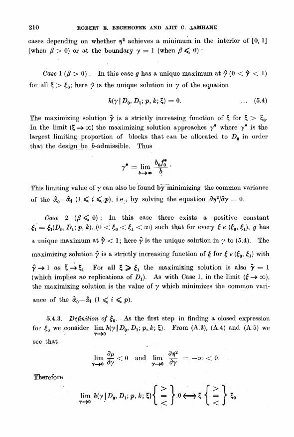
cases depending on whether ^2 achieves a minimum in the interior of [0, 1]

(when ? > 0) or at the boundary y = 1 (when ? < 0) :

Case 1 (? > 0) : In this case g has a unique maximum at y (0 < y < 1)

for all ? > ?0; here y is the unique solution in y of the equation

h(y\D0,Dx;p,k;l) = 0. ... (5.4)

The maximizing solution y is a strictly increasing function of \ for ? > ?0. In the limit (? ?> oo) the maximizing solution approaches y* where y* is the

largest limiting proportion of blocks that can be allocated to D0 in order

that the design be 6-admissible. Thus

/ = iim M. .

&- 6

This limiting value of y can also be found by minimizing the common variance

of the a0??| (1 < i ̂ p), i.e., by solving the equation dr\2\dy = 0.

Gase 2 (? ^ 0) : In this case there exists a positive constant

Ii = Si(D09 Dx; p, k), (0 < f0 < |i < oo) such that for every ? e (?0, ?J, jr has

a unique maximum at y < 1; here y is the unique solution in y to (5.4). The

maximizing solution y is a strictly increasing function of ? for ? e (?0, ?J with

y ?? 1 as ? ?

?x. For all ?> ?x the maximizing solution is also y = 1

(which implies tio replications of DJ. As with Case 1, in the limit (? ?? oo),

the maximizing solution is the value of y which minimizes the common vari

ance of the ?0? ai (1 ̂ i ^ p).

5.4.3. Definition of ?0. As the first step in finding a closed expression

f o we

see that

for |0 we consider lim A(y|D0, D^p, k; %). From (A.3), (A.4) and (A.5) we y??o

dp dw2 lim ^ < 0 and lim ~ = ?oo < 0.

7^0 oy y_>0 dy

Therefore

lim h(y\D0,Dx;p,k;l)\ = U ?=* H = K0

I < J I < J

where ?0 =

ij0(Dx;p, k) is defined by

?p (p-\)t d lim -7~

L 9 V l+p J * L ? V

(l+/>)(l+2p) l+2p J '

We evaluate this limit in Appendix A2 and show it to be

7 vx~rrnxT~"W i-r^y ? i

i- */~E?U-l I <>? v

i+p\l+P J J (5.5)

fo = 4^-1)^-2(011/3) V-^-

- (5"6)

Note that ?0 depends only on Dx but does not depend on D0. Since Dx is

either a BIB or a RB design between the p test treatments, we can substitute

A<x> = bxk(k-l)lp(p-l) in (5.6) to obtain

?o=|l?^0|l/8)V-^=^- .- M * *

(fe?1)77"

Remark 5.1 : It is known (see, e.g., Gupta, 1963) that O0(0|l/3) = 1,

Ox(0|l/3) = 1/2, O2(0|l/3) = l/4+(l/27r)arc sin (1/3), and O3(0| 1/3) = 1/8+

(3/47r)arc sin(l/3); Oi(011/3) has been computed to five decimal places for t

= 1(1)12 by Gupta (1963, Table II, p. 817).

The values of f0 for p =

2(1)6, k = 2 are 0-7979, 1-6926, 2-5214, 3-2894

and 4-0073, respectively, while ?0 = 1-4658 for p

= 3, fc = 3.

5.4.4. Definition of ?x. For Case 2, we define ?x as the smallest value

of ? for which y equals unity; hence for ? ^ ?x we have y = 1. Thus ?x is

the solution in ? of the equation

h(y\D0,Dx;p,k]C)\y=x = 0.

In general |x depends on both D0 and Dx. The value of ?x for p = 3, & = 3

is 4-5081.

5.4.5. Uniqueness of maximum of g as a function of y. As mentioned

in Section 5.4.2, we have not yet proved analytically the existence of a unique maximum for g as a function of y when ?0 < ? < oo (nor was the corresponding result proved in Bechhofer (1969) or Bechhofer and Nocturne (1972)); however,

all of our numerical calculations and certain analytical considerations point to this conclusion.

We have computed g as a function of y for selected values of ??, and given

the results in Tables 5.1 A and 5.IB to illustrate Cases 1 and 2, respectively. Table 5.1 A is for p

= k = 2 (with generator designs [DQ, Dx} of (3.1)), and

Table 5.IB is for p = k = 3 (with generator designs {J90, Dx] of (3.5)); these

computations give representative pictures of the behaviour of g as a function

of y. The behavior of g in Table 5.1 A is analogous to that of g in Figure 1

of Bechhofer (1969) in that g has a unique maximum at y < y* for ? > ?0.

However, unlike the situation in Figure 1 where lim g == 1/2? we now have

lim g depending on ? and other parameters of the design. 7-*l

5.5. Solution to the problem of obtaining continuous optimal designs. We now describe the method of solution to the problem of obtaining conti

nuous optimal designs.

(a) If Case 1 holds or if Case 2 holds but % < \x (see comment below), then solve simultaneously the two equations

h(y\D0,Dx;p,k;l) = 0 ... (5.8)

jcfrf a^?1^1e?(g) = l^? ... (5.9) -oo L yl- p J

for y and E, the solutions being y and |; here h, r?2 and yo are given by (5.3),

(A.l) and (A.2), respectively.

TABLE 5.1A. VALUES OF g AS FUNCTION OF y FOR SELECTED ? FOR p = A; = 2 (CASE 1 : ?0

= 0.7979)

7 ?

0.0 0.1 0.2 0.3 0.4 0.5 0.6 0.7 0.8 0.9 1.0

0.5 .5000 .4794 .4680 .4569 .4451 .4321 .4174 .4004 .3802 .3558 .3251

2.0 .5000 .5731 .5993 .6161 .6272 .6334 .6352 .6321 .6231 .6063 .5780

TABLE 5.1B. VALUES OF g AS A FUNCTION OF y FOR SELECTED f for p

= k = 3 (Case 2 : f0 ? 1.4658, ?-

= 4.5081)

0.0 0.1 0.2 0.3 0.4 0.5 0.6 0.7 0.8 0.9 1.0

1.0 .5000 .4707 .4561 .4431 .4305 .4179 .4049 .3914 .3774 .3625 .3468

3.0 .5000 .5879 .6196 .6407 .6556 .6661 .6730 .6769 .6779 .6762 .6716

5.0 .5000 .6978 .7639 .8059 .8350 .8560 .8712 .8822 .8897 .8944 .8965

(b) If Case 2 holds and \ ^ ?x, then solve only (5.9) for ? with y -?

1,

the solutions being y = 1, and |.

BALANCED TREATMENT INCOMPLETE BLOCK DESIGNS 21a

To see whether or not | < ?x = 4-5081 for p

= k = 3 for any specified

I?a, it is useful to note that g = 0-8561 for |

= $x

= 4-5081 which is cal

culated by evaluating (2.5). Thus IS?i iff l~aS 0-8561.

5.6. Use of tables of continuous optimal designs for p =

2(1)6, k = 2

and p =

3, k = 3. For given (_p, k) and {D0, DJ, tables of continuous optimal

designs can be computed using the method described in Section 5.5. This

has been done for p =

2(1)6, k = 2for {D0, DJ given by(3.1) and for p = k = 3

for {DQ, Dx) given by (3.5). The results are summarized in Table 5.2 which

for 1-a = 0-80, 0-90, 0-95, 0-99 gives y and f

Table 5.2 is intended for large values of 6 (which occur when aja is small

and/or 1?a is close to unity). The table is to be used as follows : (p, k),

{D0, Dx] and a*2 are given and the experimenter specifies a and 1? a. Entering

the table with (p, k, 1?a) the experimenter obtains y and the associated ?.

Then 6 = int[(?<r/a)2/ft]. Finally, /0 is chosen so that 60/0/6

~ y and b0fQ+bxfx is as close as possible ( ̂ )6. This process yields an approximately optimal

discrete design with associated confidence coefficient of approximately 1?a.

The approximations referred to in the paragraphs above arise because

we use a discrete design which is as "as close as possible" to the optimal conti

nuous design. These approximations become increasingly more accurate as 6

increases. The goodness of the approximation is assessed in the next section.

5.7. Comparison of exact and approximate optimal designs. To indicate

the accuracy of the approximation provided by the continuous optimal designs we computed the exact discrete optimal design and the corresponding conti

nuous optimal design for p = 2, k = 2, ajcr =0-2 and selected values of 6

(and thus ?). The results are displayed in Table 5.3. We compared the

approximate discrete optimal design obtained from the continuous optimal

design (by the procedure described in the preceding paragraph) and found

that it is the same as the corresponding exact discrete optimal design in every case listed in Table 5.3. We would expect that the continuous optimal

designs will provide excellent approximations to the corresponding discrete

optimal designs even for relatively small values of f (associated with low

values of confidence coefficients). Our computations have shown that the

(/-function is quite flat in the neighborhood of its maximum. As a reuslt,

g for a discrete optimal design is only slightly smaller than d for the corres

ponding continuous optimal design.

2l4 ROBERT E. BECHHOFER AND AJ?T C. TAJ?HAN?

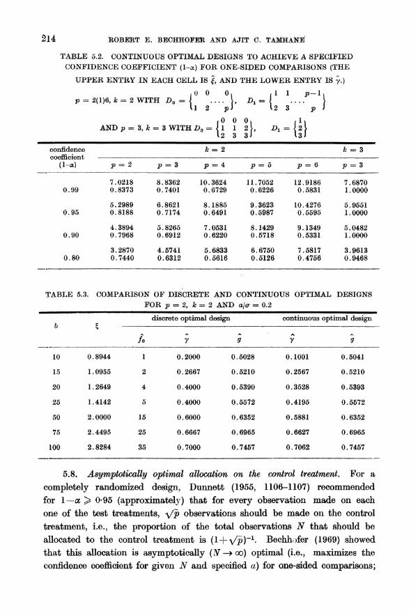
TABLE 5.2. CONTINUOUS OPTIMAL DESIGNS TO ACHIEVE A SPECIFIED CONFIDENCE COEFFICIENT (1-a) FOR ONE-SIDED COMPARISONS (THE

UPPER ENTRY IN EACH CELL IS ?, AND THE LOWER ENTRY IS y.)

,0 0 O. ,1 1 p-l\ p =

2(1)6, ?; = 2 WITH J50 = . >, A

= I

. \

ll 2 p) 12 3 pi ,0 0 0.

flj AND p = 3, k = 3 WITH D0 = I 1 1 2 V, JOj = i 2 }

confidence k = 2 & = 3 coefficient -

(1-a) jo = 2 p = 3 p

= 4 p = 5 ^ = 6 ?> = 3

7.0218 8.8362 10.3624 11.7052 12.9186 7.6870 0.99 0.8373 0.7401 0.6729 0.6226 0.5831 1.0000

5.2989 6.8621 8.1885 9.3623 10.4276 5.9551 0.95 0.8188 0.7174 0.6491 0.5987 0.5595 1.0000

4.3894 5.8265 7.0531 8.1429 9.1349 5.0482 0.90 0.7968 0.6912 0.6220 0.5718 0.5331 1.0000

3.2870 4.5741 5.6833 6.6750 7.5817 3.9613 0.80 0.7440 0.6312 0.5616 0.5126 0.4756 0.9468

TABLE 5.3. COMPARISON OF DISCRETE AND CONTINUOUS OPTIMAL DESIGNS FOR p

= 2, k = 2 AND ajcr

= 0.2

discrete optimal design continuous optimal design b I

fa y g y ?

10 0.8944 1 0.2000 0.5028 0.1001 0.5041

15 1.0955 2 0.2667 0.5210 0.2567 0.5210

20 1.2649 4 0.4000 0.5390 0.3528 0.5393

25 1.4142 5 0.4000 0.5572 0.4195 0.5572

50 2.0000 15 0.6000 0.6352 0.5881 0.6352

75 2.4495 25 0.6667 0.6965 0.6627 0.6965

100 2.8284 35 0.7000 0.7457 0.7062 0.7457

5.8. Asymptotically optimal allocation on the control treatment. For a

completely randomized design, Dunnett (1955, 1106-1107) recommended

for 1?a > 0-95 (approximately) that for every observation made on each

one of the test treatments, ^/p observations should be made on the control

treatment, i.e., the proportion of the total observations N that should be

allocated to the control treatment is (1 + Vp)"1- Bechhofer (1969) showed

that this allocation is asymptotically (N ?> oo) optimal (i.e., maximizes the

confidence coefficient for given N and specified a) for one-sided comparisons;


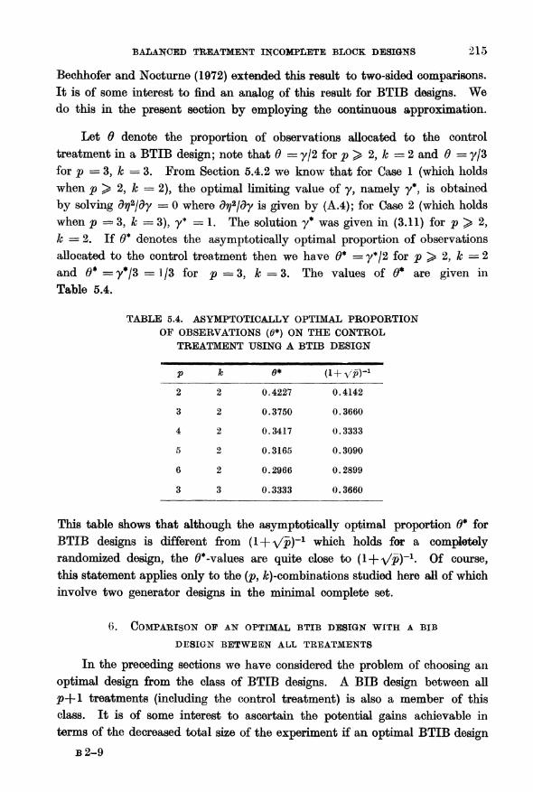
Bechhofer and Nocturne (1972) extended this result to two-sided comparisons. It is of some interest to find an analog of this result for BTIB designs. We

do this in the present section by employing the continuous approximation.

Let 6 denote the proportion of observations allocated to the control

treatment in a BTIB design; note that d = y/2 for p > 2, k = 2 and 6 =

y/3 for p = 3, k = 3. From Section 5.4.2 we know that for Case 1 (which holds

when p > 2, k = 2), the optimal limiting value of y, namely y*, is obtained

by solving dr?2jdy = 0 where dr?2jdy is given by (A.4); for Case 2 (which holds

when p = 3, k =

3), y* = 1. The solution y* was given in (3.11) for p > 2,

k = 2. If 6* denotes the asymptotically optimal proportion of observations

allocated to the control treatment then we have d* = y*/2 for p > 2, k = 2

and 0* =y*/3 =1/3 for jp = 3, & == 3. The values of 0* are given in

Table 5.4.

TABLE 5.4. ASYMPTOTICALLY OPTIMAL PROPORTION OF OBSERVATIONS (6*) ON THE CONTROL

TREATMENT USING A BTIB DESIGN

p k 6* (1+V^)"1

2 2 0.4227 0.4142

3 2 0.3750 0.3660

4 2 0.3417 0.3333

5 2 0.3165 0.3090

6 2 0.2966 0.2899

3 3 0.3333 0.3660

This table shows that although the asymptotically optimal proportion 0* for

BTIB designs is different from (1 + Vp)'1 which holds for a completely randomized design, the 6*-values are quite close to (I + Vp)'1- Of course,

this statement applies only to the (p, ̂ -combinations studied here all of which

involve two generator designs in the minimal complete set.

6. Comparison of an optimal btib design with a bib

design between all treatments

In the preceding sections we have considered the problem of choosing an

optimal design from the class of BTIB designs. A BIB design between all

p+l treatments (including the control treatment) is also a member of this

class. It is of some interest to ascertain the potential gains achievable in

terms of the decreased total size of the experiment if an optimal BTIB design

B2-9

216 ROBERT E. BECHHOFER A?TD AJlT C. TAMHAN?

is used instead of the corresponding BIB design; it is assumed here that

(p, k), {D0, DJ are given and aja and 1?a are specified. In this section we

make such a comparison for large 6; thus continuous approximations can be

used, and the problem of existence of designs for a given 6 can be ignored.

We first note that in the case of BIB designs, (2.2), (2.4), and (2.7)

simplify to

varfo-?*} =

5^T (1(x), ... (6.3)

respectively. Denote by Obib the minimum number of blocks required, to

guarantee a specified confidence coefficient 1?a using a BIB design. Then

obib is given by solving the equation

Wik-l)pk =(a^/kbJcrW(k-l)lpk =c,

2 pc2<r2 i.e., bBiB =

(?ZT)di-> - (6-4)

where c = Cp.i-j, is the solution of the equation

J *2>(*+c)d*(a:) = 1-a. ... (6.5) ? OD

The values of c have been tabulated by Bechhofer (1954), Gupta (1963) and

Milton (1963) for selected values of p and 1?a; Bechhofer's ? equals c while

Gupta's and Milton's H equals c\<\/2.

Denote the corresponding minimum number of blocks required, using the

optimal BTIB design by $btib- Note that b?TTB is given by

Sbt/r = 02

... (6.6)

A. where ? is given in Table 5.2.

For given (p, k), {D0, Dx}, a2 and specified a and 1?a we define the

efficiency of a BIB design relative to that of an optimal BTIB design by

ReJ? =(i)2^ ... (6.7)

Since a BIB design is a special case of BTIB designs we see that the relative

efficiency (RE) is <; 1. The values of RE for selected (p, k) and 1?a are

listed in Table 6.1.

TABLE 6.1. EFFICIENCY OF A BIB DESIGN RELATIVE TO AN OPTIMAL BTIB DESIGN

confidence coefficient (1-a)

0.80 0.90 0.95 0.99

2 2 0.9892 0.9684 0.9557 0.9420

3 2 0.9729 0.9414 0.9228 0.9027

4 2 0.9581 0.9201 0.8979 0.8737

5 2 0.9454 0.9029 0.8783 0.8512

6 2 0.9346 0.8887 0.8623 0.8330

3 3 0.9729 0.9423 0.9267 0.9109

From Table 6.1 we note that for fixed k and 1?a, RE decreases as p

increases; also for fixed p and k, RE decreases as 1?a increases. Thus it is

seen that substantial improvements in efficiency (i.e., savings in the total

number of blocks) can be achieved by using an optimal BTIB design instead

of the corresponding BIB design.

7. Acknowledgment

The authors are pleased to acknowledge wi+h thanks the efforts of Mr.

Carl Emont who spent long hours computing the tables of discrete optimal

designs given in Section 4. This article was completed while the second

author was spending his sabbatical leave at Cornell University during 1982-83.

This research was supported by U.S. Army Research Office?Durham Contract

DAAG-29-81-K-0168 and Office of Naval Research Contract N00014-75-C-0586

at Cornell University.

Appendix 1

Proof of Theorem 3.1 : For mathematical convenience and without loss

of generality we shall regard y =/060/6 as a continuous variable taking values

in the interval (0, 1]. (We use the same continuous approximation in Section

5.) For p = 2, k = 2 and p = 3, k = 3 we substitute A0 =/0A[)0),

Aj =/0A(l0)+/iA(11), 6 -/0&0+/A and/0 =6y0/6 in (2.6) and (2.4) to obtain

_ F60{y(61A<1o)-60^)+61A<0o))+60A^}

and

respectively. It follows that

dp -bAWW_ 0 fA 3)

for bx, A^> > 0, and therefore p is strictly decreasing in y (and hence in /0). Next we have

___!__k\jr(y)_ 5r A<V{r_p(Mi0)-Mi1))+6iAg))]+i)Mi1)}2

" ' { '

where

#7) - r2(Mi1)-Mi0)~6iA^)[p(61Af~60A^))+^

-2y60A</>[MM_0)-M_^ ... (A.5)

Since lim rf = oo, it follows that rf must be decreasing, at least in a small

y ?*o

neighborhood of y = 0+; thus it suffices to show that rf has at most one

stationary point in (0, 1], i.e., that the equation r?r(y) = 0 has at most one

root in (0, 1].

Since the constant term ? _?(60A (1))2 in (A.5) is negative, a necessary (but

clearly not sufficient) condition for both roots of ijr(y) to be real, positive and

distinct is that the coefficients of y2 and y in t}r(y) be negative and positive,

respectively, i.e., we require that

p(bxW-b0A[?)+bxW < 0.

Therefore,

djrjy) dy

y=l

The latter inequality shows that \?r(y) is increasing at y = 1. This together

with the fact that x?r(y) ?> ? oo as y ?> ?00 implies that at most one root of

i?r(y) must be in (0, 1].

The proof of the theorem now follows easily since Case 1 or Case 2 holds

depending on whether or not

sgn { ̂ ; } = sgn{^(y) |,_-} = sgnfo/?}

ly=l

is > 0 or < 0, respectively, where ? is given by (3.9). If Case 1 holds then

rf first decreases and then increases with /0 (i.e., y) while p always decreases

with /0. Hence there exists a critical number /J which is the smallest value

of/0 at which r?2 starts increasing (for fixed 6). Thus/J is the smallest value

of/0 satisfying r/2(f0) > V2(fo~d) where d is the smallest positive integer such

that d60/61 is a positive integer. If/* ^/^, then clearly designs with /0 > /* are inadmissible. If Case 2 holds then since both r?2 and p are strictly decreas

ing in f0 (i.e., y), all designs D =/o#o U/i^i ^^ /o > 0 are admissible.

Proof of Theorem 3.2 : We can express r2 of (2.3) and p of (2.4) as

?o Wo(Mr+p[Mr-Mn)+?>} (A.6)

? ._ /?(Mf-M^+M?) . A P ~/o(Mf+Mi?>-W)+K1)'

'" { '

r'2 and p' have analogous expressions with /0 replaced by f'0 and 6 replaced

by 6'.

We shall show that 6 < b' and ?>>/>' implies that r2 > r'2. From

p > />' and (A.7) we get that /06-/06' > 0, i.e.,/0//0 < 6/6' < 1. Therefore

we have

fo-fo>0- - (A.8)

Now using (A.7) and (A.8) we shall show that r2 > r'2, i.e., we shall show

that

ifo-MfJoM+WpX??) > A^fJ0(b-bf)pAM?bf~f0%)B] ... (A.9)

where A = bxA^+bx?^~b0?^ and B =

61A^)+i>(61A(?)-60A(1)). We consider

the cases p > 2, & = 2 and ^> = 3, k = 3 separately.

(7a5e 1 (# > 2, fc =2) : Using (3.2) and (3.3) we obtain 4 = 2>(i>?3)/2, 5 =

-^-(-i)^. Substituting in (A.9) for A, B and for 6, 6' from (3.4) we

find after a lengthy algebraic manipulation that (A.9) will follow if we show

that

(/?-/o)(/o/o+?'/i/?+/o/i+/o/?)+(?'-l)/o/o(/i-/i)>0. ... (A.lu)

Now note that 6'?6 > 0 yields

Ji~fi > ~~

(v__i) \Jo~fo)>

and since from (A.8) we have/??f0 > 0, (A.10) will follow if we show that

PfJi+fofi+fofi-fofo>0. .- (A.11)

220 ROBERT E. BECHHOFER AND A JIT C. TAMHANE

We use the bounds /0 < 6y*/60,/0 < b'y*jb where y* is given by (3.11) to

obtain the following bound on fx (and an analogous bound on f[) :

{ Vp+i

p -

) /

A> <

/o

p> 2,p^3, k =2

p = 3, k = 2.

(A.12)

Thus a lower bound on the Lh.s. of (A. 11) will be obtained by substituting

in it (A.12) (and an analogous bound on f[). It is easy to verify that this

substitution yields a lower bound on the lii.s. of (A.12) of exactly zero which

completes the proof of this case.

Gase 2 (p = 3, k =

3) : Using (3.6) and (3.7) we obtain A = 0, B = ? 4.

Substituting these in (A.9) we find that (A.9) will follow if we show that

Mffi-m <&'. (A.13)

36(/o-/o)

But the l.h.s. of (A.13) is less than

4(/o26-/o2&)/3&(/o-/o) < 4(/o+/o)/3 < 8/0/8 < 3/; < V

which completes the proof of this case and the theorem. In the preceding

line of the proof we have used the inequalities /0 </o and 6 < 6'.

Appendix 2

Derivation of Results in Section 5

Evaluation and simplification of dgjdy. From (2.7) and the definition of g

given in Section 5.2 we obtain by direct calculation

f vVl

x ,vi_,pvm. ge.)-(? v?+t

){ivi-P__%_) -j iv-p)

dx.

{AM)

BAXANCE?) TREATMENT ?NCOMP?J?TE BLOCK DESIGNS 221

In (A.14), $( ) denotes the standard normal p.d.f., <D(-) denotes the standard

normal c.d.f., rf =dr?jdy = (\j2y?)drfjdy where drfjdy is given by (A.4), and

p' =dpjdy is given by (A.3). After some simplification (A.14) can be written

as

Hi - ^JL_ [ ?V f*-if_^t?l? f ̂ Vp+i I 6(r)dx dy

- 2^(i~p2T372? Vplxq>p [ yV?^r l-f7T=p"J

^{l)dx

-mv-P)-vpy*^ m**) .

... (A.1?)

Making the change of variables

(A. 15) can be expressed as

dg _ p i vy _ r svy . f

... (A.16)

where

(A.17)

_j1= J y*v-\yWymy)?y, ... (A.18) ? oc

_78= f *v-HyWy)f{y)<ly, ... (A.19) ? oc

and 0*(?/) denotes <?>((y?S)?R). We now evaluate J^ and _52. Integrating

by parts in Ex with ?7 = *-9"%)^*(j/) and dF =y<f>(y)dy we obtain

,1=JF*1+T,|+(P"1? '" (A,20)

where

B? = J *M</)0WW?/. - (A.21)


From (A.20) we have

s (P-D& ?l~ W+??*+ B*+l E*

Substituting (A. 22) in (A. 16) we obtain

dg _ p ff Sifp'

.. (A.22)

4^-mi^-{-[^^+imi-p)-1^]Bt

vY(p-i) E.

)

By developments similar to those in Bechhofer (1969) we can write

(A.23)

E* B

T*( S

Vb?+? rWB*+i *p-i

V(2B*+l)(3B*+l)

B* B*+ t)

.. (A.24)

8 V{2&+l)2n \ V2?2+l/

v 2L V(2B*+1){

Bz ZB2+ ?] -1X3^+1)1

... (A.25)

Substituting E2 and Ez from (A.24) and (A.25) in (A.23), and replacing B and 8 by their definitions in (A. 17) we obtain

1+pl

"*" V?nf?+d M * >

i+p/ *-*l 7 * (1+pvT+M I i+2/> J ? T(l+P) 1+P

2 MyiDo.D^pîi)

where A(y | Z>0, Z^; #, ?fc; ?) is given by (5.3).

Evaluation, of the limit in expression (5.5) for ?0 : We note from (A.1) and

(A.2) that lim n2 =oo and Urn p = 1. Since Op-Ô 11/2) = 1/p we have t?>o y??o

from (5.5) that

* _j>(y-l)^-2(0|l/3)lim 1

' dy

?3^ 1 w2 "

Lîrj I. ... (A.26)

BALANCED TREATMENT INCOMPLETE BLOCK DESIGHS 22:1

Using (A.3) and (A.4) we write

?- = --_ Jlw {r(MT-MT+M(S')+MT}3/ii ,A 27v df f{y) v A<?> {yMb^-b^+b^+pb^}-

- ^ ''

dy

where ^r(y) is given by (A.5). Using (A.2) and (A.3) we write

jp_ _ __ _?_ __ _ft Ad, ?/*-__? M2(M'?>-M)+Mt?a+2M}-i/*. Vl~2 ?<AiN-y r(M(o)_6oA(,)+M(o,)+6oAa,

... (A.28)

Combining (A.27) and (A.28) we obtain

V

{y(M(?)-M(i)+&iA(g))+M(I;}{y_p(??iA(^-M(l))+ftiA(g)]+j>M(i>} 11/2

7[2(M<?>-&0?<?>)+M<o>]+2M<j> J

... (A.29)

Since lim \[r(y) = ?

jo^A*^)2 we have ?-40

X

9' dp

lim -^3-?- =*V-????T--

- (A-30)

Substituting (A.30) in (A.26) we obtain the desired result (5.6).

References

Bechhofer, R. E. (1969) : Optimal allocation of observations when comparing several treat

ments with a control. Multivariate Analysis, II (Ed. P. R. Krishnaiah), New York, :

Academic Press 463-473.

Bechhofer, R. E. and Nocturne, D. J. M. (1972) : Optimal allocation of observations when

comparing several treatments with a control (II) : 2-sided comparisons. Technometrics,

14, 423-436.

Bechhofer, R. E. and Tamhane, A. C. (1981) : Incomplete block designs for comparing treat

ments with a control : General Theory, Technometrics, 23, 45-57. Corrigendum, Techno

metrics, 24, 171.

- (1983) : Tables of admissible and optimal balanced treatment incomplete block

(BTIB) designs for comparing treatments with a control. To appear in Selected Tables in

Mathematical Statistics.

B2-10

224 tt?B?R? ? feteCHHOF?R AN?) AJ?T C. TA?HAN?

Gupta, S. S. (1963) : Probability integrals of multivariate normal and multivariate t. Ann.

Math. Statist., 34, 792-828.

Milton, R- C- (1933) : Tables of the equally correlated multivariate normal probability

integral. Tech. Rep. No. 27, Dept. of Statistics, Univ. of Minnesota, Minneapolis, MN.

Notz, W. I. and Tamhane, A. C. (1983) : Balanced treatment incomplete block (BTIB) designs

for comparing treatments with a control : Minimal complete sets of generator designs for

k = 3, p =

3(1)10. Communications in Statistics, Ser A, to appear.

Pearce, S. C. (1960) : Supplemented balance. Biometrika, 47, 263-271.

Paper received : July, 1980.

Revised : December, 1982.

indian statistical institute - northwestern universityusers.iems.northwestern.edu/~ajit/papers/6)...

Documents