INCORPORATING LEVEL OF EFFORT PARADATA IN THE

NSDUH NONRESPONSE ADJUSTMENT PROCESS

Contract No. HHSS283200800004C RTI Project No. 0211838.108.106.010

Authors:

Paul P. Biemer Patrick Chen Kevin Wang

Project Director:

Thomas G. Virag

Prepared for:

Substance Abuse and Mental Health Services Administration Rockville, Maryland 20857

Prepared by:

RTI International Research Triangle Park, North Carolina 27709

June 2013

This page intentionally left blank.

INCORPORATING LEVEL OF EFFORT PARADATA IN THE

NSDUH NONRESPONSE ADJUSTMENT PROCESS

Contract No. HHSS283200800004C RTI Project No. 0211838.108.106.010

Authors:

Paul P. Biemer Patrick Chen Kevin Wang

Project Director:

Thomas G. Virag

Prepared for:

Substance Abuse and Mental Health Services Administration Rockville, Maryland 20857

Prepared by:

RTI International Research Triangle Park, North Carolina 27709

June 2013

Acknowledgments This publication was developed for the Substance Abuse and Mental Health Services Administration (SAMHSA), Center for Behavioral Health Statistics and Quality (CBHSQ), by RTI International (a trade name of Research Triangle Institute), Research Triangle Park, North Carolina, under Contract No. HHSS283200800004C. Significant contributors at RTI include Paul Biemer, Patrick Chen, and Kevin Wang. Michelle Back copyedited the report, and Thomas G. Virag is the RTI Project Director.

v

Table of Contents

Chapter Page

1. Introduction ......................................................................................................................... 1

2. Background ......................................................................................................................... 5

3. Data ..................................................................................................................................... 7

4. Model and Notation ............................................................................................................ 9

5. Parameter Estimation ........................................................................................................ 11

6. Extensions to the Basic Model .......................................................................................... 13

7. Measures of Nonignorable Bias ........................................................................................ 17

8. Application to the National Survey on Drug Use and Health ........................................... 19 8.1. Approach ............................................................................................................... 19 8.2. Results for Screener Variables .............................................................................. 22 8.3. Results for Substantive Variables ......................................................................... 25 8.4. Estimates and Standard Errors of GEM and GEM+ Models ................................ 27

9. The Quality of the NSDUH Callback Data....................................................................... 33

10. Conclusions ....................................................................................................................... 37

References ..................................................................................................................................... 39

Appendix

A Investigation of Call Record Data Properties ................................................................. A-1

vi

This page intentionally left blank.

vii

List of Figures

Figure Page

1. Graphs of the Relationship Between ∆ and |Bias| for 20 Response Propensity Strata for Hispanicity, Sex, Age, and Race ....................................................................... 25

viii

This page intentionally left blank.

ix

List of Tables

Table Page

1. Data Summary for Callback Model .................................................................................... 8

2. Prevalence Estimates for Sex, Ethnicity, Age, and Race, by Model and Screener .......... 23

3. Nonignorable Bias for Sex, Ethnicity, Age, and Race, by Model .................................... 24

4. Variable Names and their Definitions for the Analysis of Substantive Variables ............ 26

5. Model 0 Estimates of Prevalence for the Substantive Variables and the Bias Estimated by the Five Models (in Percent) among Persons Aged 12 or Older ................ 27

6. Additional Variables for Analysis of Estimates and Standard Errors ............................... 29

7. Weight Distribution for the NSDUH Sample ................................................................... 29

8. Estimates, Standard Errors, and Mean Square Errors of GEM and GEM+ Model among Persons Aged 12 or Older ..................................................................................... 31

x

This page intentionally left blank.

1

1. Introduction The National Survey on Drug Use and Health (NSDUH) is the primary source of

statistical information on the use of illegal drugs, alcohol, and tobacco by the U.S. civilian, noninstitutionalized population aged 12 or older. Conducted by the Federal Government since 1971, the survey collects data through face-to-face interviews with a representative sample of the population at the respondent's place of residence. Since 1990, the survey has been conducted annually with separate samples drawn each year. The survey is sponsored by the Substance Abuse and Mental Health Services Administration (SAMHSA), U.S. Department of Health and Human Services, and is planned and managed by SAMHSA's Center for Behavioral Health Statistics and Quality (CBHSQ). The annual conduct of NSDUH is paramount in meeting a critical objective of SAMHSA's mission to maintain current data on the prevalence of substance use in the United States.

To continue producing data that are accurate and on a timely basis, SAMHSA's CBHSQ must update NSDUH periodically to reflect changing substance use and mental health issues. CBHSQ is planning to implement changes related to a partial NSDUH redesign. These changes include use of a new sample design in 2014 and a limited update to the interview questionnaire in 2015. The new sample design will allow for continued national, State, and substate-level estimation comparable with estimations from previous surveys. The sample design's improved efficiency will result in significant cost savings. The primary change to the questionnaire is an updated set of prescription drug modules, which will include current prescription drugs and incorporate a new questionnaire structure. Other planned changes to the questionnaire include a revised health module that contains new questions about drug and alcohol screening by primary care physicians. These changes will seek to achieve three main goals: (1) to revise the questionnaire to address changing policy and research data needs, (2) to modify the survey methodology to improve the quality of estimates and the efficiency of data collection and processing, and (3) to maintain trends in core substance use estimates across survey years.

SAMHSA's planned changes for the NSDUH in 2014 and 2015 also provide an opportunity to investigate new and innovative approaches to nonresponse adjustment that may have the potential of improving overall NSDUH data quality in the face of declining response rates for both the NSDUH and surveys in general. This report describes the results of an investigation of the callback modeling approach for adjusting for nonresponse. Current NSDUH nonresponse adjustments assume that the nonresponse mechanism is ignorable. Nonresponse adjustments using the callback model described in this report attempt to reduce the nonignorable nonresponse bias. If successful, this approach will improve the NSDUH data quality by reducing the bias due to nonresponse.

The report is organized as follows. In the remainder of this section, we present a general description of the callback modeling approach for nonresponse adjustment. Section 2 provides a brief review of the callback modeling literature and describes prior applications of the methodology used in this study. Section 3 describes the data requirements for applying the callback model methodology with particular emphasis on the NSDUH data used in our analysis. The NSDUH call record data used to measure interviewing effort is described in some detail.

2

Section 4 formally presents the statistical model and notation developed for the approach and Section 5 derives the maximum likelihood estimators of the model parameters. Section 6 considers several important extensions of the basic model proposed in Section 4 that are required for the NSDUH application. As a by-product of the estimation approach, several measures of nonignorable nonresponse are derived in Section 7. In Section 8, the methodology developed in the previous sections are applied to the NSDUH data described in Section 3. Section 9 discusses some issues associated with the callback level of effort data used in the analysis that may explained the somewhat disappointing results provided in Section 8. Finally, in Section 10, we provide our conclusions and recommendations for further research.

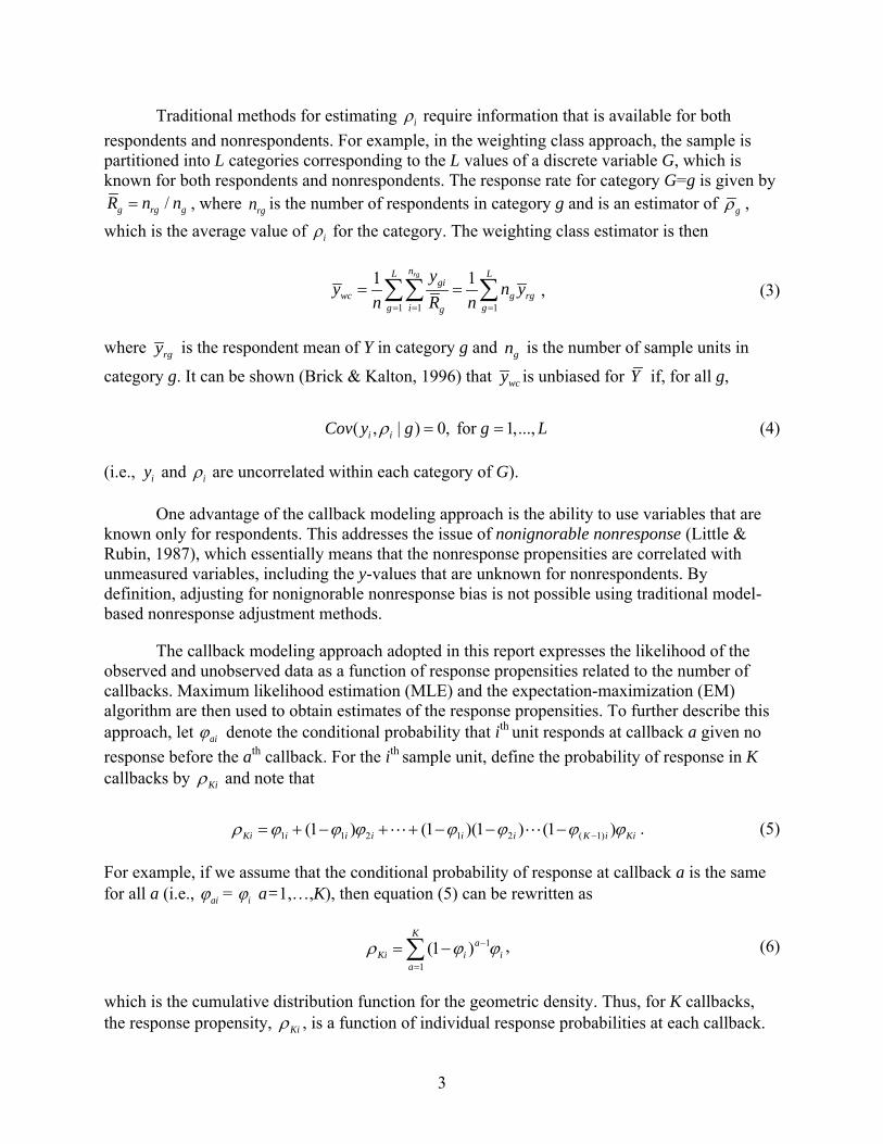
In most sample surveys, response propensity weighting is used to compensate for unit nonresponse that is related to refusals, noncontacts, and other causes. Response propensity weighting reduces nonresponse bias by weighting a responding unit by the inverse of its probability of responding to the survey. This is analogous to the Horvitz-Thompson estimator that weights a unit by the inverse of its probability of selection in the sample.

Suppose a simple random sample (SRS) of size n is selected and the value of the survey variable Y, denoted by yi, is observed for all respondents. Let Ri denote the response indicator variable for the ith sample unit, which is equal to 1 if the unit responds to the survey and to 0 if the unit does not respond. Let r ii

n R=∑ denote the number of respondents in the sample. Let Yi

denote the characteristic value for the ith population member, and let 11

Nii

Y N Y−=

= ∑ denote the

population mean to be estimated. A natural estimator of Y is the sample mean of observations given by

1

rn

ii

rr

yy

n==∑

. (1)

However, this estimator is biased unless ( , ) 0i iCov R y = ; that is, unless there is no relationship between the propensity to respond and the outcome variable (see Lessler & Kalsbeek, 1992). Lessler and Kalsbeek show that

1

1 rni

adji i

yyn ρ=

= ∑ (2)

is an unbiased estimator, where ( | )i iE R iρ = and where ( | )iE R i denotes expectation over the hypothetical response propensity distribution for the ith sample member. Note that ρi can also be written as Pr( 1| )iR i= or the probability the ith unit responds to the survey. The ρi 's are often called response propensities in the survey literature and are unknown in practical applications. The usual approach is to estimate them using a weighting class approach or a response propensity model. The ρi 's in equation (2) are then replaced by their estimates (e.g., Biemer & Christ, 2008). Roughly speaking, a callback is an attempt to obtain a response from a sampling unit. A callback model uses information on the number of such attempts and their outcomes to estimate the response propensities, ρi , and ultimately to adjust the estimators for nonresponse.

3

Traditional methods for estimating ρi require information that is available for both respondents and nonrespondents. For example, in the weighting class approach, the sample is partitioned into L categories corresponding to the L values of a discrete variable G, which is known for both respondents and nonrespondents. The response rate for category G=g is given by /g rg gR n n= , where nrg is the number of respondents in category g and is an estimator of ρg , which is the average value of ρi for the category. The weighting class estimator is then

1 1 1

1 1rgnL Lgi

wc g rgg i gg

yy n y

n R n= = =

= =∑∑ ∑ , (3)

where yrg is the respondent mean of Y in category g and ng is the number of sample units in

category g. It can be shown (Brick & Kalton, 1996) that ywc is unbiased for Y if, for all g,

( , | ) 0, for 1,...,i iCov y g g Lρ = = (4)

(i.e., yi and ρi are uncorrelated within each category of G).

One advantage of the callback modeling approach is the ability to use variables that are known only for respondents. This addresses the issue of nonignorable nonresponse (Little & Rubin, 1987), which essentially means that the nonresponse propensities are correlated with unmeasured variables, including the y-values that are unknown for nonrespondents. By definition, adjusting for nonignorable nonresponse bias is not possible using traditional model-based nonresponse adjustment methods.

The callback modeling approach adopted in this report expresses the likelihood of the observed and unobserved data as a function of response propensities related to the number of callbacks. Maximum likelihood estimation (MLE) and the expectation-maximization (EM) algorithm are then used to obtain estimates of the response propensities. To further describe this approach, let ϕai denote the conditional probability that ith unit responds at callback a given no response before the ath callback. For the ith sample unit, define the probability of response in K callbacks by ρKi and note that

1 1 2 1 2 ( 1)(1 ) (1 )(1 ) (1 )Ki i i i i i K i Kiρ ϕ ϕ ϕ ϕ ϕ ϕ ϕ−= + − + + − − − . (5)

For example, if we assume that the conditional probability of response at callback a is the same for all a (i.e., ϕai = ϕi a=1,…,K), then equation (5) can be rewritten as

1

1(1 )

Ka

Ki i ia

ρ ϕ ϕ−=

= −∑ , (6)

which is the cumulative distribution function for the geometric density. Thus, for K callbacks, the response propensity, ρKi , is a function of individual response probabilities at each callback.

4

Now suppose G is known only for respondents and assume group homogeneity (i.e., the conditional response probabilities are equal for all units in the same group). Mathematically, this is written as φai = φag , say, for all units i in category g for g=1,..,L. To further simplify the discussion, assume that conditional probabilities of the response are equal for all callbacks (i.e., φag =φg for a=1,…,K) so that the response probabilities take the form of equation (6) and let ρKg denote the common response probability in group g. Let nag denote the number of units in group g that respond at the ath call attempt. Under these assumptions, the data 1 2( , ,..., )g g Kgn n n follow a multinomial distribution with parameters ng and ρag , g=1,…,L, and a=1,…,K. The log-likelihood kernel is, therefore, given by

1 1log( )

K L

ag g aga g

n π ρ= =

=∑∑L , (7)

where π g is the proportion of the population in category g. This likelihood can be maximized using a variety of methods, including the EM algorithm (Dempster, Laird, & Rubin, 1977) to obtain estimates of the parameters π g and φg , g=1,..,L. In particular, let π̂ g denote the MLE of π g . Then, nπ̂ g can replace ng in equation (3) to obtain the estimator

1

ˆL

cb g rgg

y yπ=

=∑ . (8)

To obtain an expression for the variance of y , we use the first order Taylor series approximation. Let Ωπ̂ denote the variance–covariance matrix for the vector ˆ ˆ[ ]gπ=π and let

[ ]rgy=ry , where

1/

rgn

rg gi rgi

y y n=

=∑ is the simple expansion mean of all observations in group g, g

= 1,...,K. An approximate expression of the variance of y is

2

1V( ) V( ) E( ) E( )

K

g rgg

y yπ=

′≈ +∑ r π ry Ω y (9)

(Biemer & Link, 2007), which is estimated by substituting the appropriate estimators for the parameters in equation (8) by

2

1

ˆˆ( ) ( )K

g gg

v y v yπ=

′= +∑ πyΩ y . (10)

When Y is a categorical variable, it can replace the grouping variable G in equation (8). In that case, the estimates of the proportion in category y of Y are given by ˆ yπ , which are the estimates from the callback model. Moreover, the estimator is model unbiased since the covariance in equation (4) and conditional on y is 0. This is an important special case that will be explored in this report.

5

2. Background The idea of using data on respondent availability and contact difficulty to adjust for

nonignorable nonresponse bias has been around for more than 60 years. Politz and Simmons (1949) used a throwaway idea by Hartley (1946) to develop a famous method of adjustment based upon retrospective reports of availability. Although the Politz and Simmons adjustment was rather crude, it clearly demonstrated that contact difficulty was related to many characteristics and could be used to reduce nonresponse bias. These early ideas led to a callback modeling framework for nonresponse adjustment that encompasses two distinctly different approaches: regression modeling and probability modeling.

The regression modeling approach (Alho, 1990; Anido & Valdéz, 2000; Wood, White & Hotopf, 2006) is an extension of the traditional response propensity logistic regression model. This approach models an individual's propensity to respond at each attempt. Using a modified conditional likelihood estimation approach, the model incorporates partially missing data as well as fully observed predictors at each attempt. The model predicts the response propensity for each respondent that can then be used to build a nonresponse adjusted weight. By using partially observed data, the model adjustment can compensate for nonignorable and ignorable nonresponse. Extensions of the basic approach include the use of probit rather than the logistic distribution (Anido & Valdéz, 2000) and models that incorporate Bayesian priors (Wood, et al, 2006).

The probability modeling approach (Drew & Fuller,1980; Potthoff, Manton, & Woodbury, 1993; Biemer & Link, 2007) is similar in that it too uses a modified maximum likelihood method to obtain the estimates. However, rather than modeling response propensity, the approach specifies a model for the probability that an observation falls into a particular cell of the data summary table (see Table 1 in Chapter 3 for more details), which is the cross-classification of the dependent variable, the number of contact attempts, and the contact outcomes. It does not directly estimate an overall response propensity; rather it simultaneously estimates probabilities of contact and probabilities of interview based on contact as well as the population proportions in each category of a survey characteristic. These parameter estimates can be used to build nonresponse adjustment weights if desired. It employs the expectation-maximization (EM) algorithm to address the incomplete predictors. Since it too uses partially observed variables, it provides adjustments for nonignorable nonresponse.

One criticism of both modeling approaches is their simplifying assumptions that seldom hold for practical applications. For example, most of the models provide only for the probability of contacting a sample member, ignoring the probability that the sample member consents to an interview conditional upon the contact. The models often assume that the probability of a contact and interview does not vary by callback attempt. In addition, there has been no rigorous evaluation of the bias reduction capabilities of the approaches, relying instead on simulations, applications to artificial populations, and model fit diagnostics to gauge the viability of the approaches. Biemer and Link (2007) provides one attempt to apply a callback model to a set of real data and address some of the problems associated with applications of callback modeling to actual field work.

6

Biemer and Link (2007) extended the probability modeling approach proposed by Drew and Fuller (1980). Their method used level of effort (LOE) indicators based on call attempts to model the relationship between response propensity, LOE, and nonresponse bias for key outcome variables. In most surveys, call history data are available for all sample members, including nonrespondents, and since the LOE required to interview a sample member is likely to be highly correlated with response propensity, this method is ideally suited for modeling the nonignorable nonresponse. Biemer and Link (2007) applied their approach to data for a random-digit dialing (RDD) telephone survey.

The rest of this report presents the results of analyses in which the Biemer and Link (2007) methodology is applied to data from the 2006 National Survey on Drug Use and Health (NSDUH). In this research, two key questions are addressed. First, we want to determine whether callback models can be used to evaluate the quality of the current NSDUH nonresponse adjustment. Second, we want to determine whether the current NSDUH nonresponse adjustment approach can be improved by incorporating callback information into the adjustment process, and if so, how much improvement is possible. Chapter 3 discusses some relevant data set details for our study.

7

3. Data The methods used in this report were adapted from Biemer and Link (2007) for the

National Survey on Drug Use and Health (NSDUH). To facilitate developing the model described in the next chapter, we will briefly review the structure of NSDUH data used in our analysis.

The NSDUH interview process consists of a household screener used to enumerate household members and identify eligible respondents, followed by the selection of up to two members of the household for an interview. Interviews are conducted primarily using audio computer-assisted self-interviewing (ACASI), but some items (mostly demographic) are gathered through computer-assisted personal interviewing (CAPI). In 2006, 137,057 households were screened and interviews were conducted with 67,802 respondents. The weighted screener response rate was 90.6 percent and the weighted interview response rate was 74.4 percent.

Thus, the NSDUH has unit nonresponse at two levels: the screening interview and the main interview. The focus of this report is on the latter (referred to as the main interview). Because the main interview nonresponse rate is lower, the potential for nonresponse bias is higher for this type of nonresponse. Although this has not yet been attempted, the methods discussed in this report could also be applied to adjust for screener nonresponse. The observations used for analysis come from all 85,034 screener respondents that were successfully screened and selected for an interview.

Our analysis uses information that is entered by interviewers for each visit to a sampled dwelling unit. Interviewers enter case status information into the record of calls (ROC) data using a handheld computer. Collected data elements include the interim or final outcome of the call (e.g., noncontact, refusal, completed screening, completed interview, etc.) and an open-ended notes field. The time and day of the call attempt are automatically recorded by the handheld computer. Results are transmitted daily to a central database and can be reviewed by an interviewer's supervisors in a Web-accessible case management system (CMS). Interviewers use the ROC data to record information that can help with case management and scheduling.

Records in the ROC data that did not reflect actual visits were removed from the data for our analyses. For example, final result codes for main interview nonresponse cases are entered into the ROC data after review and approval by a field supervisor and do not result from a visit by the interviewer and were, therefore, removed from the data.

NSDUH interviewers may attempt to contact and interview a sample member numerous times before further attempts are terminated and the case is closed out. All sample cases are ultimately categorized into a number of final case dispositions. For our purposes, these dispositions have been collapsed further into four main types: (1) interviewed, (2) final refusal, (3) final nonresponse other than refusal (e.g., language barriers, physically or mentally unable, or unavailable), or (4) censored. Dispositions (1), (2), and (3) are self-explanatory. Disposition (4), censored cases, are essentially noncontacted cases that have been terminated prematurely because either they are no longer needed for the sample (e.g., sample size requirements have been met) or it is no longer cost effective, efficient, or viable to pursue them. For example, at the

8

end of the field period, cases that have not received disposition (1), (2), or (3) are categorized as (4), censored, regardless of their number of attempts. Because censored cases can contribute information on nonresponse, we will consider ways of using them in the analysis.

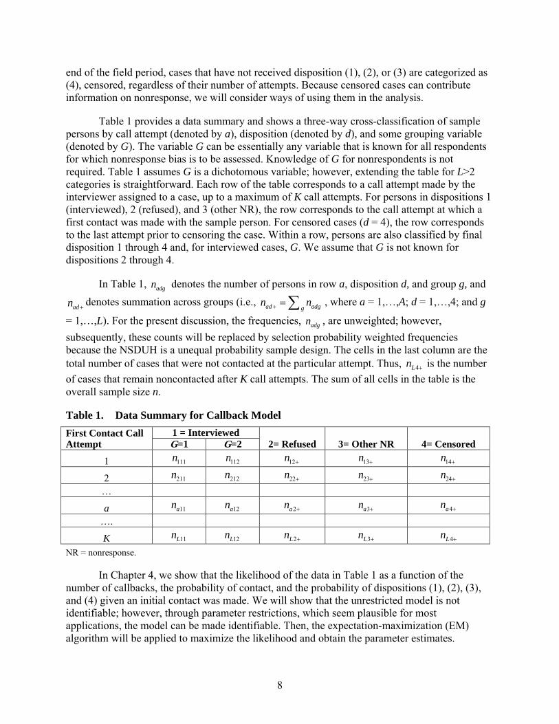
Table 1 provides a data summary and shows a three-way cross-classification of sample persons by call attempt (denoted by a), disposition (denoted by d), and some grouping variable (denoted by G). The variable G can be essentially any variable that is known for all respondents for which nonresponse bias is to be assessed. Knowledge of G for nonrespondents is not required. Table 1 assumes G is a dichotomous variable; however, extending the table for L>2 categories is straightforward. Each row of the table corresponds to a call attempt made by the interviewer assigned to a case, up to a maximum of K call attempts. For persons in dispositions 1 (interviewed), 2 (refused), and 3 (other NR), the row corresponds to the call attempt at which a first contact was made with the sample person. For censored cases (d = 4), the row corresponds to the last attempt prior to censoring the case. Within a row, persons are also classified by final disposition 1 through 4 and, for interviewed cases, G. We assume that G is not known for dispositions 2 through 4.

In Table 1, adgn denotes the number of persons in row a, disposition d, and group g, and adn + denotes summation across groups (i.e., ad adgg

n n+ =∑ , where a = 1,…,A; d = 1,…,4; and g

= 1,…,L). For the present discussion, the frequencies,

adgn , are unweighted; however, subsequently, these counts will be replaced by selection probability weighted frequencies because the NSDUH is a unequal probability sample design. The cells in the last column are the total number of cases that were not contacted at the particular attempt. Thus, 4Ln + is the number of cases that remain noncontacted after K call attempts. The sum of all cells in the table is the overall sample size n.

Table 1. Data Summary for Callback Model First Contact Call Attempt

1 = Interviewed 2= Refused 3= Other NR 4= Censored G=1 G=2

1 111n 112n 12n + 13n + 14n +

2 211n

212n 22n +

23n + 24n +

… a 11an 12an 2an + 3an +

4an + …. K

11Ln 12Ln

2Ln + 3Ln +

4Ln +

NR = nonresponse.

In Chapter 4, we show that the likelihood of the data in Table 1 as a function of the number of callbacks, the probability of contact, and the probability of dispositions (1), (2), (3), and (4) given an initial contact was made. We will show that the unrestricted model is not identifiable; however, through parameter restrictions, which seem plausible for most applications, the model can be made identifiable. Then, the expectation-maximization (EM) algorithm will be applied to maximize the likelihood and obtain the parameter estimates.

9

4. Model and Notation For ease of exposition, we assume simple random sample (SRS) of size n households is

selected from a population of size N households and later extend these results for complex survey sampling. Extending the notation in equation (5), let agα denote the probability a person in group g is contacted at call attempt a for a = 1,…,K, and let adgβ for d=1,..,3 denote the conditional probability that a person in group g is classified to final disposition d at attempt a given the person is contacted at attempt a.

Several schemes can be used to define a "contact" and the "final disposition." For example, a contact could correspond to the first contact with the sample person, first contact with any household member, or the last contact with the household or sample person. Likewise, a final disposition could be defined for sample person or household. The meanings of these terms can vary across applications depending what scheme best describes the data likelihood. In our experience, good results have been obtained assuming that the contact attempt refers to the attempt at which first contact was made with the sample member. The following pending interview result codes were considered contacts: appointment for interview, breakoff (partial interview), physically/mentally incompetent, language barrier (Spanish), language barrier (other), refusal, and parental refusal (for 12 to 17 year olds). Noncontact pending interview result codes were No One at Dwelling Unit, Respondent Unavailable, and Other.1 This intuitively makes sense because the number of attempts to obtain the first contact would provide predictability of the likelihood for contacting a person. Other issues to consider in the definition of a contact attempt will be discussed in Section 8.1.

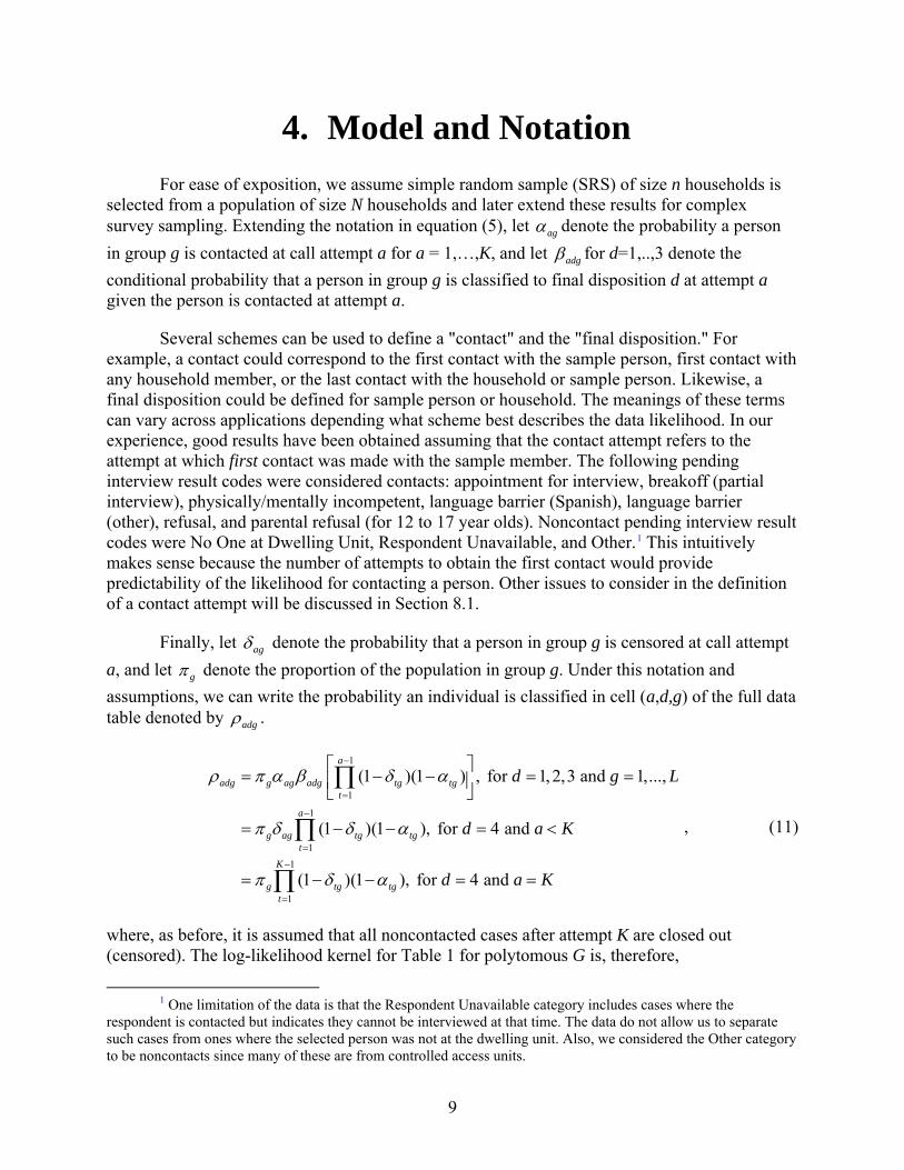
Finally, let agδ denote the probability that a person in group g is censored at call attempt a, and let gπ denote the proportion of the population in group g. Under this notation and assumptions, we can write the probability an individual is classified in cell (a,d,g) of the full data table denoted by adgρ .

1

1

1

11

1

(1 )(1 ) , for 1, 2,3 and 1,...,

(1 )(1 ), for 4 and

(1 )(1 ), for 4 and

a

adg g ag adg tg tgt

a

g ag tg tgt

K

g tg tgt

d g L

d a K

d a K

ρ π α β δ α

π δ δ α

π δ α

−

=

−

=

−

=

= − − = =

= − − = <

= − − = =

∏

∏

∏

, (11)

where, as before, it is assumed that all noncontacted cases after attempt K are closed out (censored). The log-likelihood kernel for Table 1 for polytomous G is, therefore,

1 One limitation of the data is that the Respondent Unavailable category includes cases where the

respondent is contacted but indicates they cannot be interviewed at that time. The data do not allow us to separate such cases from ones where the selected person was not at the dwelling unit. Also, we considered the Other category to be noncontacts since many of these are from controlled access units.

10

4

1 11 1 1 2 1

log logK G K L

a g a g ad adga g a d g

n nρ ρ+= = = = =

= +∑∑ ∑∑ ∑ . (12)

Note that, in this likelihood, the response probabilities are summed over the L groups as

1

L

adgg

ρ=∑

for dispositions (2), (3), and (4) because we assume that only the sums, adggn∑ , are known for

noninterviewed persons.

In general, the number of cells in Table 1 is K(L+4), which is the maximum number of parameters that can be estimated. The data likelihood for Table 1 contains many more than K(L+4) parameters and is, therefore, not identifiable unless some parameter restrictions are imposed. A number of restrictions will be considered in the application. However, one that seems practical for the National Survey on Drug Use and Health (NSDUH) application is to reduce the number of censoring probabilities. For many surveys, the decision to terminate further effort on a case does not depend on the grouping variable, G, particularly in cases where G is a questionnaire variable (Y) and is unknown during fieldwork. In such cases, G does not influence censoring and it may be plausible to assume that the probability of censoring is the same for all groups (i.e., ag aδ δ= for g =1,…,L). It may also be plausible to assume that the censoring probabilities are the same across call attempts:

1(1 )aaδ δ δ −= − . (13)

Both of these assumptions can be tested. For example, cases requiring greater numbers of call backs may be censored with higher probabilities because they would be more likely to still be active toward the end of the survey when most censoring occurs. In addition, some groups G are more difficult to contact than the others and may require more callbacks to finalize. Such cases would also seem to be more likely to be censored. Fortunately, if the number of censored cases is small (as it is in the NSDUH), then it is unlikely that a significant reduction in model fit will be observed by restricting the censoring probabilities as shown in equation (13).

Finally, we will consider restrictions on the disposition probabilities, adgβ , to further reduce model complexity and achieve model identifiability. In other studies (e.g., Groves & Couper, 1998), contact difficultly is not strongly related to the ultimate cooperation (i.e., persons that are difficult to contact are often not more likely to refuse nor are persons who are easy to contact more likely to cooperate in the survey). This means that it may be plausible to assume that adg dgβ β= for a=1,…,K, d=1,2,3 and g=1,…,L, which saves an additional 2L(K-1) parameters. This assumption can be tested for a subset of call attempts; however, this more simplified model provides a reasonable starting point for an identifiable model. With this assumption combined with the restrictions on gaδ , the model has (K+3)L-1 parameters and the model becomes identifiable as long as K is greater than L. In practical applications, these restrictions are usually not sufficient, however, since these ignore 0 frequency cells, which also create identifiability issues, particularly when K is large relative to the sample size. In those cases, the α and β parameters can be further restricted, usually with little loss of model fit. Some plausible approaches for this will be explored in the application.

11

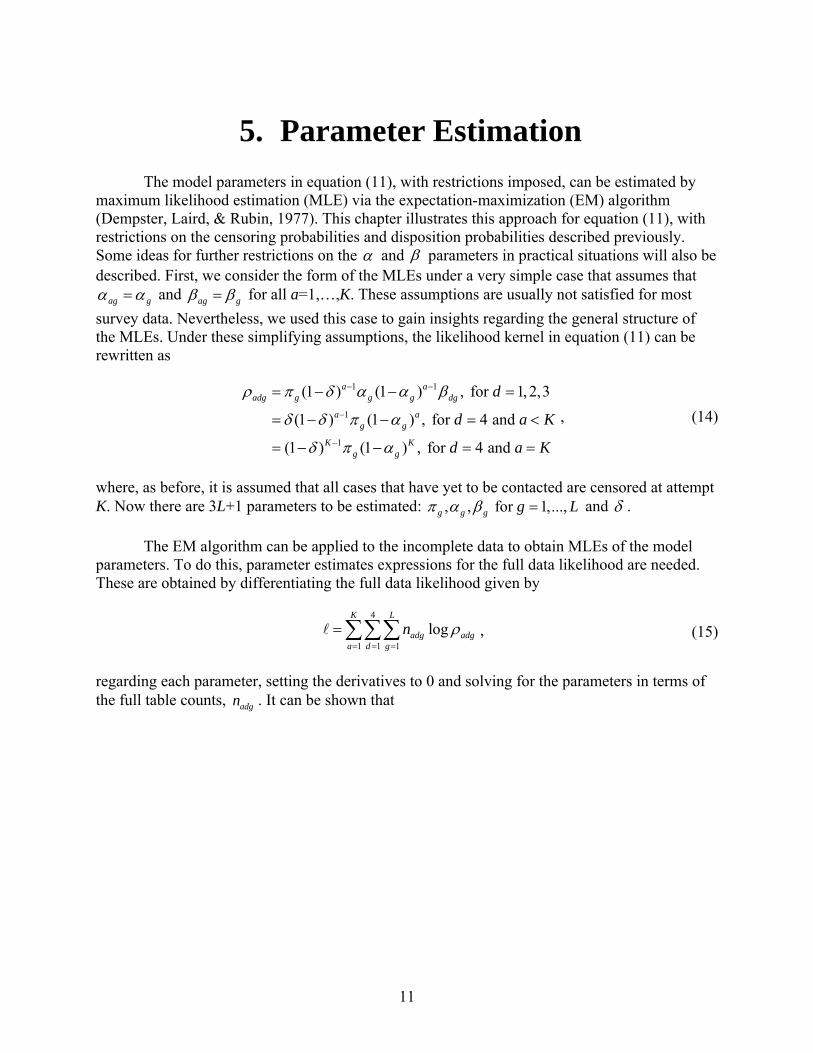
5. Parameter Estimation The model parameters in equation (11), with restrictions imposed, can be estimated by

maximum likelihood estimation (MLE) via the expectation-maximization (EM) algorithm (Dempster, Laird, & Rubin, 1977). This chapter illustrates this approach for equation (11), with restrictions on the censoring probabilities and disposition probabilities described previously. Some ideas for further restrictions on the α and β parameters in practical situations will also be described. First, we consider the form of the MLEs under a very simple case that assumes that

ag gα α= and ag gβ β= for all a=1,…,K. These assumptions are usually not satisfied for most survey data. Nevertheless, we used this case to gain insights regarding the general structure of the MLEs. Under these simplifying assumptions, the likelihood kernel in equation (11) can be rewritten as

1 1

1

1

(1 ) (1 ) , for 1, 2,3

(1 ) (1 ) , for 4 and

(1 ) (1 ) , for 4 and

a aadg g g g dg

a ag g

K Kg g

d

d a K

d a K

ρ π δ α α β

δ δ π α

δ π α

− −

−

−

= − − =

= − − = <

= − − = =

, (14)

where, as before, it is assumed that all cases that have yet to be contacted are censored at attempt K. Now there are 3L+1 parameters to be estimated: , , for 1,...,g g g g Lπ α β = and δ .

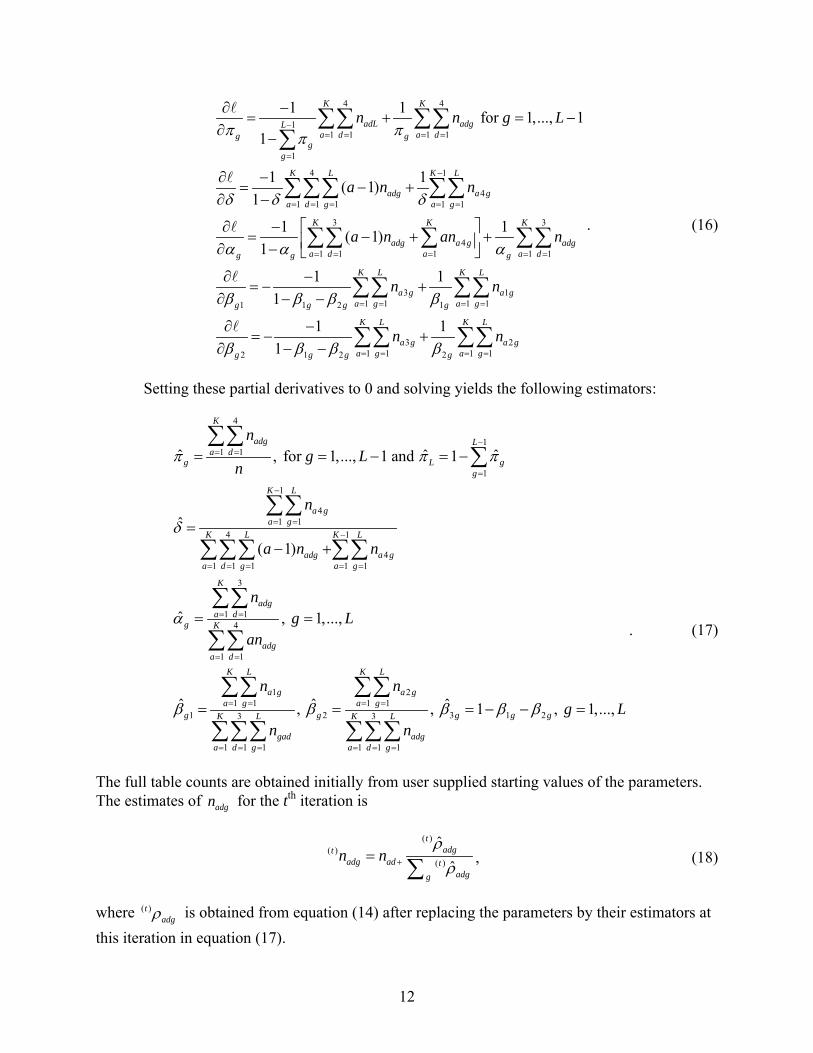
The EM algorithm can be applied to the incomplete data to obtain MLEs of the model parameters. To do this, parameter estimates expressions for the full data likelihood are needed. These are obtained by differentiating the full data likelihood given by

4

1 1 1log

K L

adg adga d g

n ρ= = =

=∑∑∑ , (15)

regarding each parameter, setting the derivatives to 0 and solving for the parameters in terms of the full table counts, adgn . It can be shown that

12

4 4

11 1 1 1

1

4 1

41 1 1 1 1

3 3

41 1 1 1 1

1 1

1 1 for 1,..., 11

1 1( 1)1

1 1( 1)1

11

K K

adL adgLa d a dg g

gg

K L K L

adg a ga d g a g

K K K

adg a g adga d a a dg g g

g

n n g L

a n n

a n an n

π ππ

δ δ δ

α α α

β β

−= = = =

=

−

= = = = =

= = = = =

∂ −= + = −

∂ −

∂ −= − +

∂ −

∂ − = − + + ∂ −

∂ −= −

∂ −

∑∑ ∑∑∑

∑∑∑ ∑∑

∑∑ ∑ ∑∑

3 1

1 1 1 12 1

3 21 1 1 12 1 2 2

1

1 11

K L K L

a g a ga g a gg g g

K L K L

a g a ga g a gg g g g

n n

n n

β β

β β β β

= = = =

= = = =

+−

∂ −= − +

∂ − −

∑∑ ∑∑

∑∑ ∑∑

. (16)

Setting these partial derivatives to 0 and solving yields the following estimators:

4

11 1

1

1

41 1

4 1

41 1 1 1 1

3

1 14

1 1

11 1

1 3

1 1 1

ˆ ˆ ˆ, for 1,..., 1 and 1

ˆ( 1)

ˆ , 1,...,

ˆ ,

K

adg La d

g L gg

K L

a ga g

K L K L

adg a ga d g a g

K

adga d

g K

adga d

K L

a ga g

g K L

gada d g

ng L

n

n

a n n

ng L

an

n

n

π π π

δ

α

β

−= =

=

−

= =−

= = = = =

= =

= =

= =

= = =

= = − = −

=− +

= =

=

∑∑∑

∑∑

∑∑∑ ∑∑

∑∑

∑∑

∑∑

∑∑∑

21 1

2 3 1 23

1 1 1

ˆ ˆ , 1 , 1,...,

K L

a ga g

g g g gK L

adga d g

ng L

nβ β β β= =

= = =

= = − − =∑∑

∑∑∑

. (17)

The full table counts are obtained initially from user supplied starting values of the parameters. The estimates of adgn for the tth iteration is

( )( )

( )

ˆˆ

tadgt

adg ad tadgg

n nρρ+=

∑ , (18)

where ( )tadgρ is obtained from equation (14) after replacing the parameters by their estimators at

this iteration in equation (17).

13

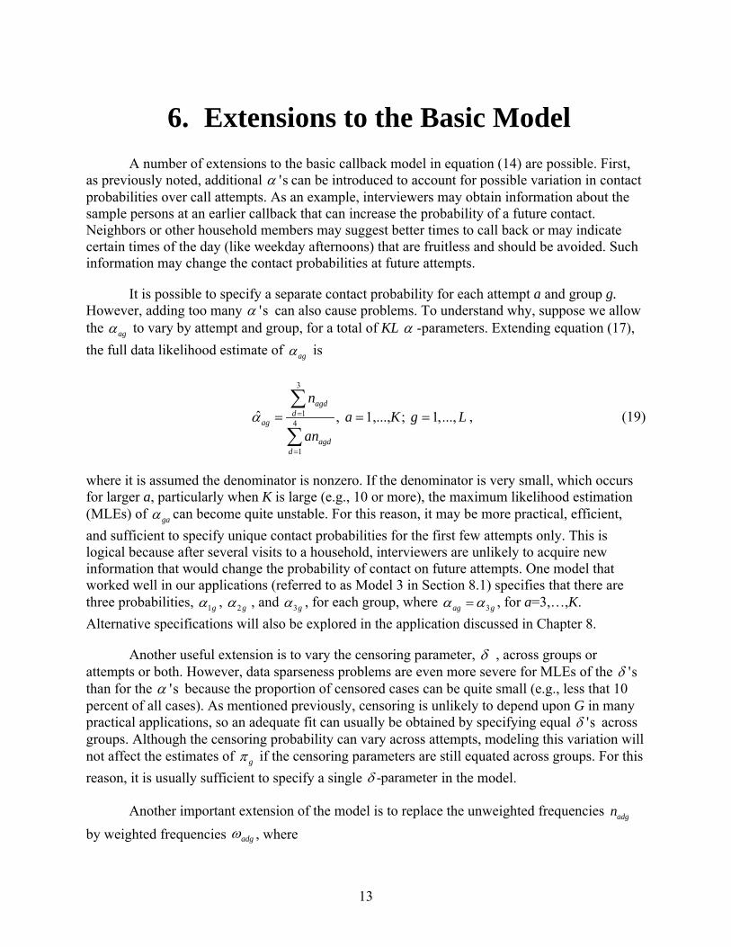
6. Extensions to the Basic Model A number of extensions to the basic callback model in equation (14) are possible. First,

as previously noted, additional 'sα can be introduced to account for possible variation in contact probabilities over call attempts. As an example, interviewers may obtain information about the sample persons at an earlier callback that can increase the probability of a future contact. Neighbors or other household members may suggest better times to call back or may indicate certain times of the day (like weekday afternoons) that are fruitless and should be avoided. Such information may change the contact probabilities at future attempts.

It is possible to specify a separate contact probability for each attempt a and group g. However, adding too many 'sα can also cause problems. To understand why, suppose we allow the agα to vary by attempt and group, for a total of KL α -parameters. Extending equation (17), the full data likelihood estimate of agα is

3

14

1

ˆ , 1,..., ; 1,...,agd

dag

agdd

na K g L

anα =

=

= = =∑

∑, (19)

where it is assumed the denominator is nonzero. If the denominator is very small, which occurs for larger a, particularly when K is large (e.g., 10 or more), the maximum likelihood estimation (MLEs) of gaα can become quite unstable. For this reason, it may be more practical, efficient, and sufficient to specify unique contact probabilities for the first few attempts only. This is logical because after several visits to a household, interviewers are unlikely to acquire new information that would change the probability of contact on future attempts. One model that worked well in our applications (referred to as Model 3 in Section 8.1) specifies that there are three probabilities, 1gα , 2gα , and 3gα , for each group, where 3ag gα α= , for a=3,…,K. Alternative specifications will also be explored in the application discussed in Chapter 8.

Another useful extension is to vary the censoring parameter, δ , across groups or attempts or both. However, data sparseness problems are even more severe for MLEs of the 'sδthan for the 'sα because the proportion of censored cases can be quite small (e.g., less that 10 percent of all cases). As mentioned previously, censoring is unlikely to depend upon G in many practical applications, so an adequate fit can usually be obtained by specifying equal 'sδ across groups. Although the censoring probability can vary across attempts, modeling this variation will not affect the estimates of gπ if the censoring parameters are still equated across groups. For this reason, it is usually sufficient to specify a single δ -parameter in the model.

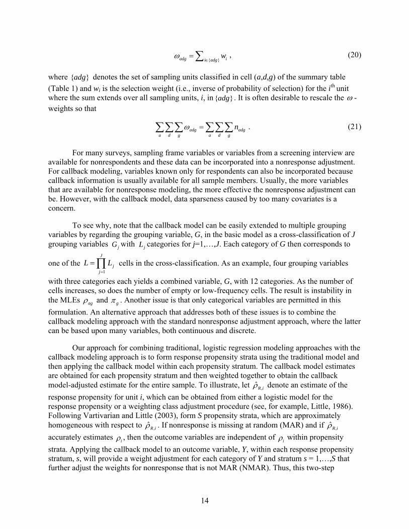
Another important extension of the model is to replace the unweighted frequencies adgnby weighted frequencies adgω , where

14

{ }adg ii adg

wω∈

=∑ , (20)

where { }adg denotes the set of sampling units classified in cell (a,d,g) of the summary table (Table 1) and wi is the selection weight (i.e., inverse of probability of selection) for the ith unit where the sum extends over all sampling units, i, in { }adg . It is often desirable to rescale the ω -weights so that

adg adg

a d g a d gnω =∑∑∑ ∑∑∑ . (21)

For many surveys, sampling frame variables or variables from a screening interview are available for nonrespondents and these data can be incorporated into a nonresponse adjustment. For callback modeling, variables known only for respondents can also be incorporated because callback information is usually available for all sample members. Usually, the more variables that are available for nonresponse modeling, the more effective the nonresponse adjustment can be. However, with the callback model, data sparseness caused by too many covariates is a concern.

To see why, note that the callback model can be easily extended to multiple grouping variables by regarding the grouping variable, G, in the basic model as a cross-classification of J grouping variables jG with jL categories for j=1,…,J. Each category of G then corresponds to

one of the

1

J

jj

L L=

=∏ cells in the cross-classification. As an example, four grouping variables

with three categories each yields a combined variable, G, with 12 categories. As the number of cells increases, so does the number of empty or low-frequency cells. The result is instability in the MLEs agρ and gπ . Another issue is that only categorical variables are permitted in this formulation. An alternative approach that addresses both of these issues is to combine the callback modeling approach with the standard nonresponse adjustment approach, where the latter can be based upon many variables, both continuous and discrete.

Our approach for combining traditional, logistic regression modeling approaches with the callback modeling approach is to form response propensity strata using the traditional model and then applying the callback model within each propensity stratum. The callback model estimates are obtained for each propensity stratum and then weighted together to obtain the callback model-adjusted estimate for the entire sample. To illustrate, let ,ˆR iρ denote an estimate of the response propensity for unit i, which can be obtained from either a logistic model for the response propensity or a weighting class adjustment procedure (see, for example, Little, 1986). Following Vartivarian and Little (2003), form S propensity strata, which are approximately homogeneous with respect to ,ˆR iρ . If nonresponse is missing at random (MAR) and if ,ˆR iρ accurately estimates iρ , then the outcome variables are independent of iρ within propensity strata. Applying the callback model to an outcome variable, Y, within each response propensity stratum, s, will provide a weight adjustment for each category of Y and stratum s = 1,…,S that further adjust the weights for nonresponse that is not MAR (NMAR). Thus, this two-step

15

approach combines traditional nonresponse adjustment modeling (e.g., using logistic regression) and callback modeling (via MLE) to obtain nonresponse adjustments that adjust for both ignorable and nonignorable nonresponse without many of the sparseness issues in callback modeling, with a large number of covariates or the restriction that all covariates should be categorical. In our example, 20 propensity strata are formed that still provides an adequate sample in each stratum for estimating the callback model parameters.

Finally, Biemer and Link (2007) and Biemer and Wang (2007) extend the callback model considered above by adding terms representing hard core nonrespondents (HCNRs) (i.e., persons who have zero response propensities and cannot be interviewed regardless of the number of call attempts). Such persons are indistinguishable in the sample from persons who have not been interviewed but have a nonzero response propensity. The authors represent the HCNR population by adding a dichotomous latent variable (say, η ) to the callback model, which is an indicator for HCNR and non-HCNR persons (i.e., η =1 for HCNR and η = 0 otherwise). This latent variable is allowed to vary by group G. In the simplest model they consider, this adds L additional parameter to the model (i.e., Pr( 1| )gη = for g=1,…,L). These additional probabilities along with the other callback model parameters can be estimated by MLE, again using the expectation-maximization (EM) algorithm. For the National Survey on Drug Use and Health (NSDUH) analysis, Biemer and Wang (2007) found little improvement in the estimates of π g for this model compared with the models considered previously that do not have this feature. Therefore, we will not consider it further for this report.

16

This page intentionally left blank.

17

7. Measures of Nonignorable Bias Using response propensity stratification in conjunction with the callback model has an

additional advantage. It also provides a test of the assumption of missing at random (MAR) invoked by traditional nonresponse adjustment approaches. Let ρsyi denote the response propensity for the ith unit in response propensity stratum s and category y of the outcome variable Y. If the MAR assumption holds for Y, then sy syρ ρ ′= for all y and y′. If this equality is rejected, so must be the MAR assumption. In this way, the callback model with response propensity stratification can be used to test the adequacy of a traditional nonresponse adjustment.

Consider a callback model with parameters syπ , say syα α= , say sβ β= , and sya sδ δ= for s=1,…,S, y = 1,…, C, and a = 1,…,K, where S is the number of response propensity strata, and C is the number of categories of Y. (This model will be referred to as Model 1 in Section 8.1.) The model specifies that the prevalence of Y varies by stratum (s) and that the contact probabilities ( syα ) vary across both the categories of Y and strata. Further, it assumes interview probabilities (

sβ and sδ ) do not depend upon Y and vary only by stratum. Let Model 0 denote Model 1 with the additional restriction that sy sα α= , for all y. Roughly speaking, Model 0 assumes that response propensities do not vary within stratum across the categories of Y (i.e., the traditional nonresponse adjustment fully compensates for nonresponse with respect to Y). This is equivalent to specifying that, conditional on s, nonresponse is MAR with respect to Y. Since Model 1 is nested within Model 0, the conditional chi-squared test can be used to test the null hypothesis

sy sα α= .

Specifically, let 0

20,dfL and

1

21,dfL denote the likelihood ratio chi-square statistics for

Models 0 and 1, respectively. The difference, 0 1

2 212 0, 1,df dfd L L= − , is distributed as a χ 2 random

variable. If 12d exceeds the (1-p)th percentile of 21Cχ − where C is the number of categories of Y,

the MAR assumption is rejected with probability 1-p, providing evidence that the MAR assumption is not valid for Y. It may also be concluded that the response propensity model used to create the S strata does not adequately adjust for the nonresponse bias in estimates from Y. In this way, the potential of nonignorable nonresponse to affect the estimates of Y after traditional nonresponse adjustments have been applied to the sampling weights can also be formally tested.

Alternative tests can also be constructed. For example, let Model 1′ denote Model 1 after relaxing the restriction on the ' sβ . In particular, assume sya syβ β= for s=1,…,S, y=1,…,C, and a=1,…,K. Since Model 1′ is also nested in Model 0, the nested chi-squared test can be used to test whether both

sy sα α= and sy sβ β= . Note that the degrees of freedom for this test is 2(C-1)

and, thus, provides a more powerful test.

18

This page intentionally left blank.

19

8. Application to the National Survey on Drug Use and Health

As described previously, the National Survey on Drug Use and Health (NSDUH) incorporates a short screening interview—referred to as the screener—followed by an hour-long substantive interview—referred to as the main interview. The screener is designed to identify youths aged 12 to 17 years and young adults aged 18 to 25 years for oversampling. In addition to age, the screener collects addition demographic variables such as sex and race/ethnicity. The main interview is subsequently conducted with a random subsample of the screener respondents.

Nonresponse can occur for both the screener and main interviews. As noted previously, for the data analyzed in this report, screener nonresponse was about 9 percent and the main interview nonresponse was about 16 percent. The NSDUH employs separate nonresponse weighting adjustments for the two types of nonresponse. For the present analysis, only the main interview nonresponse adjustment is considered. Subsequent references to nonresponse adjustments in this report pertain to the main interview only.

When performing the main interview nonresponse weight adjustment, the NSDUH uses a response propensity model that is a logit model incorporating 13 variables and selected interactions, including a number of State-specific components obtained from U.S. Census data (Chen et al., 2005). These variables include those obtained from the screener, which are available for all main interview nonrespondents. The models are fit using the Generalized Exponential Model (GEM) procedure developed by Folsom and Singh (2000). The GEM procedure also applies a calibration adjustment that poststratifies the nonresponse adjusted counts to census control totals across a number of demographic variables. The application in this chapter considers the bias in the NSDUH estimates after the nonresponse adjustment has been applied and prior to the poststratification adjustment.

The next section describes the approach we used to apply the callback models in the previous sections to the NSDUH, and then the results of the study are given the subsequent sections.

8.1. Approach

As noted in Chapter 2, two key questions were addressed by this research: (a) can callback models be used to evaluate the quality of the current NSDUH nonresponse adjustment? and (b) is it possible to improve the current NSDUH nonresponse adjustment approach by incorporating callback information into the adjustment process? To address (a), we applied a number of alternative callback models ranging from the simple to the complex. The results below focus on four models that represent the type of results we obtained and illustrate the potential of the callback modeling approach for evaluating and reducing nonignorable nonresponse in the NSDUH estimates. The four callback models are:

Model 0: gπ , agα α= , agβ β= , agδ δ= for 1,..., , 1,...,g L a A= =

20

Model 1: gπ , ag gα α= , agβ β= , agδ δ= for 1,..., , 1,...,g L a A= =

Model 2: same as Model 1, except 1 2, , 2,...,g ag g a Lα α α= =

Model 3: same as Model 1, except 1 2 3, , , 3,...,g g ag g a Lα α α α= = .

Model 0, referred to as the null model, Model 0, specifies that neither contact probabilities nor interview probabilities vary by group (i.e., gaα α= and agβ β= for g=1,…,L). This model is equivalent to the assumption of no nonignorable nonresponse bias for the variable of interest. When the response propensity strata are formed using response propensities estimated from the GEM model, the Model 0 estimates are essentially the same as the GEM estimates within each stratum. Model 1 contains 2L +1 parameters corresponding to the L-1 prevalence probabilities ( , 1,..., 1g g Lπ = − ), L contact probabilities ( , 1,...,g g Lα = ), a single interview probability β , and a single censoring probability δ . The key assumption for this model is that contact probabilities remain constant for all call attempts a. Model 2 assumes that the probability of contact for the first call attempt is unique in each group, but call attempts 2 through L share the same contact probability within each group. Thus, Model 2 contains an additional L parameter. Finally, Model 3 allows unique contract probabilities for the first two call attempts, while they are the same across attempts a = 3,…,L. Model 3, therefore, adds L more contact probability parameters to Model 2.

Models that allowed the 'sβ and 'sδ to vary across groups and call attempts were also explored. The models that varied the censoring probabilities ( 'sδ ) by group gave results that were very similar to the models where group equality was imposed. However, models that allowed the disposition probabilities ( 'sβ ) to vary by group gave results that were quite different from and considerably biased compared to models where group equality was imposed. One possible explanation for the extreme bias is error in the callback data. As we will discuss in Chapter 9, the number of call attempts recorded for a case can be inaccurate for modeling purposes. Our extensive investigations into the appropriateness of using NSDUH record of calls (ROC) data as a source of callback data suggest that interviewers tend to underreport call attempts as envisioned in the callback model. (This is discussed in more detail in Appendix A.) A limited simulation study revealed that the maximum likelihood estimation (MLEs) of the 'sβare much more affected by these recording errors than MLEs of the other model parameters. More work is needed to fully understand why. Nevertheless, models that allow the disposition probabilities to vary by group performed poorly and those results will not be presented in this report.

One additional model that incorporates callback information was considered. This is the NSDUH GEM model augmented by a new variable derived from the number of call attempts required to obtain a final disposition for a unit (referred to as the level of effort or LOE variable). This model, denoted by GEM+, and the standard GEM model (without the LOE variable) bring the number of models in the analysis to six.

Early work to apply callback models to the NSDUH (Biemer & Wang, 2007) considered a number of alternate definitions of a call attempt. A call attempt can be defined as any attempt

21

to contact and interview a respondent. However, as will be discussed later, this definition is problematic primarily because of the inaccuracy with which it is recorded by interviewers for callback modeling purposes. For example, interviewers may make several calls to the same unit within a single afternoon. Some interviewers may record each attempt separately as they should, while others may collapse these into a single attempt. Biemer and Wang (2007) found that combining multiple attempts within the same morning, afternoon, or evening (call time slots) produced somewhat better results. For the present analysis, call days (i.e., combining multiple attempts on the same day into a single attempt) offered further improvement, and this definition was used for the results presented here.

Since age, race, sex, and ethnicity are obtained in the screener interview (some by proxy response) for all main interview persons, these characteristics are known and can be used to construct gold standard estimates for the purposes of evaluating a given model's ability to adjust for nonignorable nonresponse bias. Let Y denote one of these variables and form the data summary table (Table 1), using Y to play the role of the grouping variable G. Replace the cell frequencies ( yadn ) by selection weighted counts (

yadω ) as described in Chapter 6. We then apply

the callback model to this data table to estimate: , 1,...,y y Cπ = . Let ( )ˆ myπ denote the estimate of

yπ from callback model m, where m = 0, 1, 2, 3, GEM and GEM+. Let ( )ˆ T

yπ denote the estimate based upon the full screener data, which is considered the gold standard (i.e., assume that ( )ˆ( )T

y yE π π= ). Then, the bias in the adjusted estimate from model m is

( ) ( ) ( )ˆm m Ty yB π π= − . (22)

The NSDUH GEM model includes the screener variables age, race, sex, and ethnicity, which are the Y variables for this analysis. As such, the biases for GEM and GEM+ weighted adjusted estimates for these Y's are essentially 0. This is not a fair comparison of the GEM modeling approach because we are interested in how the GEM nonresponse adjustment performs for variables that are not in the model (so-called ignored variables). This is accomplished by the leave-one-out approach, where Y is omitted from the GEM and GEM+ models for assessing the nonignorable nonresponse bias for estimates of Y.

As an example, to evaluate the nonignorable nonresponse bias for sex, this variable is omitted from the GEM model, and the nonresponse weight adjustment factors are estimated using the response propensities from the reduced model. Applying these factors to the NSDUH base weights produces nonresponse adjusted estimates of the prevalence of males (or females) in the population. Since sex is left out of the GEM model, the estimates of the prevalence of sex will be biased to the extent that the other variables in the model are unable to account for the differences in the nonresponse mechanisms for males and females. This nonignorable nonresponse bias can be estimated by equation (22) using the estimate of the prevalence of males from the screener. The nonresponse biases for the ethnicity, age, and race are computed in the same manner. In this way, we obtain insight about the performance of the GEM nonresponse adjustment for Y-variables that are ignored in the model that may be related to sex, ethnicity, age, and race. This process also provides the opportunity to evaluate how the callback modeling approach performs relative to the GEM and GEM+ models for adjusting for nonignorable nonresponse bias.

22

Finally, for reasons described in Chapter 7, the callback models (1, 2, and 3) were fit separately to 20 equally sized response propensity strata. These strata were formed using response propensities from the GEM model with the Y variable removed to simulate the situation of nonignorable nonresponse. The overall callback model estimate was then computed by weighting the estimates of ( )ˆ m

syπ for strata s=1,…,20, by the total weight in each stratum following the usual estimator for stratified sampling.

Thus, to summarize our approach for some screener variable, Y, the full GEM model (excluding Y) is used to estimate the response propensities for each unit in the sample. The units are then sorted and 20 response propensity strata of equal size are created. Within each stratum, a data summary table (like Table 1) is generated separately for sex, ethnicity, age, and race using frequencies that are weighted by the NSDUH selection probabilities. For each of these variables, the four callback models (including Model 0) were applied to the weighted data summary table in each stratum to produce the model parameters estimates. Of particular interest in this analysis are the estimates of the proportions ( )ˆ m

syπ , for s=1,…,20 and y=1,…,C for each model and the

overall estimate ( )ˆ myπ . For the callback model, the overall estimate is computed from the stratum

estimates by

( )

( )ˆ

ˆ

ms sy

m sy

ss

ω ππ

ω

+

+

=∑∑ , (23)

where sω + is the sum of the selection weights for all cases in stratum s. To obtain the corresponding GEM+ estimates for a particular screener variable, Y, the GEM model was fit after removing the Y. The nonresponse adjustment weight factors from this model were applied to the selection weights in each stratum. The GEM estimate for yπ is then

( )

( )( )

ˆ

GEMsy

GEM sy GEM

sys y

ωπ

ω

+

+

=∑∑∑

, (24)

where ( )GEMsyω + is the GEM nonresponse adjusted weight for interviewed cases in stratum s having

Y=y. The GEM+ model estimates were formed analogously using the GEM model with the LOE variable added.

8.2. Results for Screener Variables

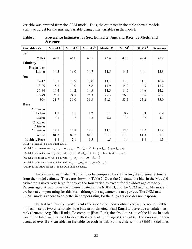
Table 2 shows the prevalence estimates for screener (Y) variables for the unadjusted model (Model 0) and the five nonresponse adjusted models in our comparison. The estimate based upon full screener information is in the last column and will be considered the gold standard for this analysis. Models 0 through 3 and the screener estimates are a weighted average for estimates over the 20 propensity strata. The GEM and GEM+ estimates were produced from models fit to the entire data set. As noted previously, for the latter models, the corresponding Y

23

variable was omitted from the GEM model. Thus, the estimates in the table show a models ability to adjust for the missing variable using other variables in the model.

Table 2. Prevalence Estimates for Sex, Ethnicity, Age, and Race, by Model and Screener

Variable (Y) Model 01 Model 12 Model 23 Model 34 GEM5 GEM+5 Screener Sex

Males 47.1 48.0 47.5 47.4 47.0 47.4 48.2 Ethnicity

Hispanic or Latino 14.3 16.0 14.7 14.5 14.1 14.1 13.8

Age 12-17 13.1 12.9 13.0 13.1 11.3 11.1 10.4 18-25 15.7 17.0 15.8 15.9 14.3 14.5 13.2 26-34 14.4 14.2 14.5 14.5 14.5 14.6 14.2 35-49 25.1 24.8 25.3 25.3 26.3 26.6 26.2

50+ 31.7 31.0 31.3 31.3 33.5 33.2 35.9 Race

American Indian 1.1 1.1 1.2 1.1 0.9 0.9 0.9 Asian 3.1 3.7 3.2 3.2 3.6 3.7 4.7

Black or African

American 13.1 12.9 13.1 13.1 12.2 12.2 11.8 White 81.3 80.2 81.1 81.1 81.8 81.8 81.3

Multiple Race 1.4 2.1 1.5 1.5 1.4 1.4 1.3 GEM = generalized exponential model. 1Model 0 parameters are gπ , agα α= , agβ β= , agδ δ= for 1,..., , 1,...,g L a A= = 2Model 1 parameters are gπ , ag gα α= , agβ β= ,

agδ δ= for 1, ..., , 1, ...,g L a A= =;

3Model 2 is similar to Model 1 but with 1 2, , 2, ...,g ag g a Lα α α= = 4Model 3 is similar to Model 1 but with, 1 2 3, , , 3, ...,g g ag g a Lα α α α= =5GEM+ is the GEM model with the LOE variable added.

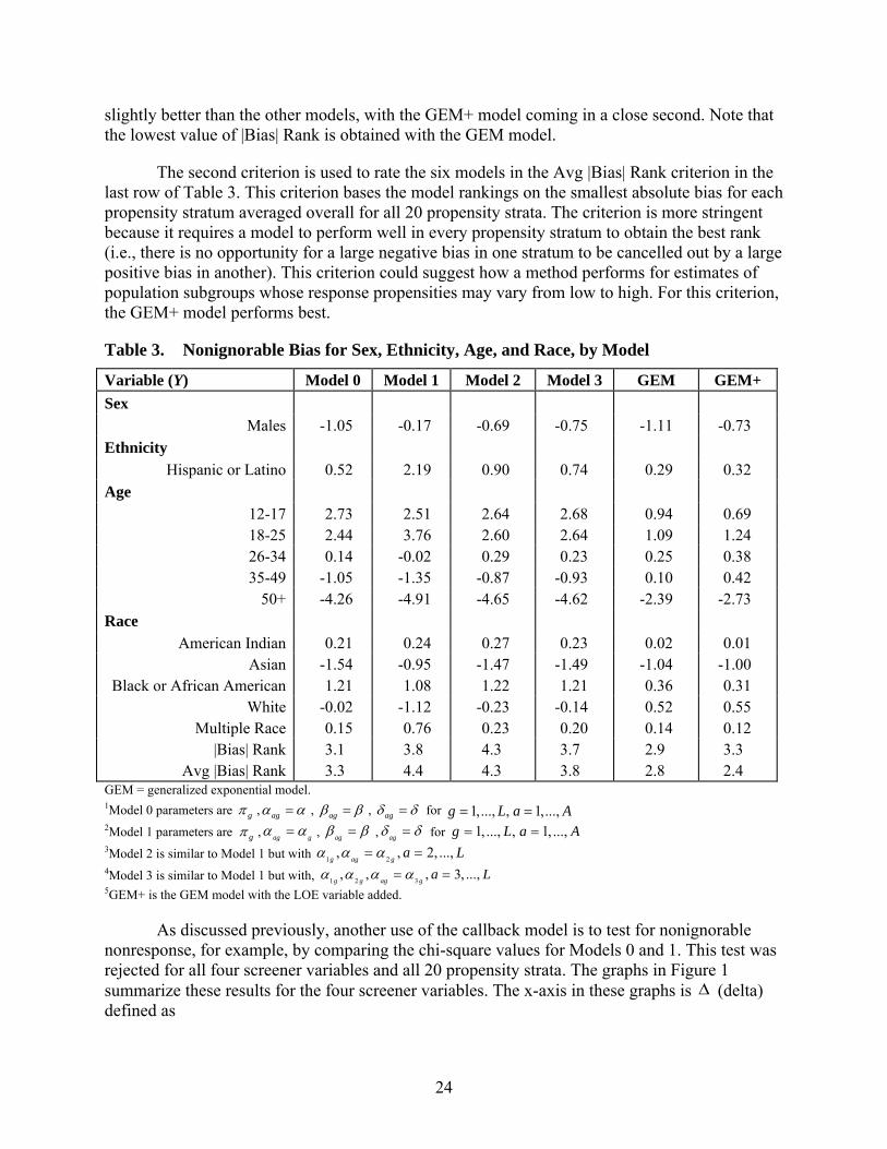
The bias in an estimate in Table 1 can be computed by subtracting the screener estimate from the model estimate. These are shown in Table 3. Over the 20 strata, the bias in the Model 0 estimator is never very large for any of the four variables except for the oldest age category. Persons aged 50 and older are underestimated in the NSDUH, and the GEM and GEM+ models are best at compensating for this bias, although the adjustment is not perfect. The GEM and GEM+ models appear to do better in compensating for the 50 years or older nonresponse.

The last two rows of Table 3 ranks the models on their ability to adjust for nonignorable nonresponse by two criteria: absolute bias rank (denoted |Bias| Rank) and average absolute bias rank (denoted Avg |Bias| Rank). To compute |Bias| Rank, the absolute value of the biases in each row of the table were ranked from smallest (rank of 1) to largest (rank of 6). The ranks were then averaged over the Y variables in the table for each model. By this criterion, the GEM model does

24

slightly better than the other models, with the GEM+ model coming in a close second. Note that the lowest value of |Bias| Rank is obtained with the GEM model.

The second criterion is used to rate the six models in the Avg |Bias| Rank criterion in the last row of Table 3. This criterion bases the model rankings on the smallest absolute bias for each propensity stratum averaged overall for all 20 propensity strata. The criterion is more stringent because it requires a model to perform well in every propensity stratum to obtain the best rank (i.e., there is no opportunity for a large negative bias in one stratum to be cancelled out by a large positive bias in another). This criterion could suggest how a method performs for estimates of population subgroups whose response propensities may vary from low to high. For this criterion, the GEM+ model performs best.

Table 3. Nonignorable Bias for Sex, Ethnicity, Age, and Race, by Model

Variable (Y) Model 0 Model 1 Model 2 Model 3 GEM GEM+ Sex

Males -1.05 -0.17 -0.69 -0.75 -1.11 -0.73 Ethnicity

Hispanic or Latino 0.52 2.19 0.90 0.74 0.29 0.32 Age

12-17 2.73 2.51 2.64 2.68 0.94 0.69 18-25 2.44 3.76 2.60 2.64 1.09 1.24 26-34 0.14 -0.02 0.29 0.23 0.25 0.38 35-49 -1.05 -1.35 -0.87 -0.93 0.10 0.42

50+ -4.26 -4.91 -4.65 -4.62 -2.39 -2.73 Race

American Indian 0.21 0.24 0.27 0.23 0.02 0.01 Asian -1.54 -0.95 -1.47 -1.49 -1.04 -1.00

Black or African American 1.21 1.08 1.22 1.21 0.36 0.31 White -0.02 -1.12 -0.23 -0.14 0.52 0.55

Multiple Race 0.15 0.76 0.23 0.20 0.14 0.12 |Bias| Rank 3.1 3.8 4.3 3.7 2.9 3.3

Avg |Bias| Rank 3.3 4.4 4.3 3.8 2.8 2.4 GEM = generalized exponential model. 1Model 0 parameters are gπ , agα α= , agβ β= , agδ δ= for 1,..., , 1,...,g L a A= = 2Model 1 parameters are gπ , ag gα α= , agβ β= ,

agδ δ= for 1, ..., , 1, ...,g L a A= =

3Model 2 is similar to Model 1 but with 1 2, , 2, ...,g ag g a Lα α α= = 4Model 3 is similar to Model 1 but with, 1 2 3, , , 3, ...,g g ag g a Lα α α α= =5GEM+ is the GEM model with the LOE variable added.

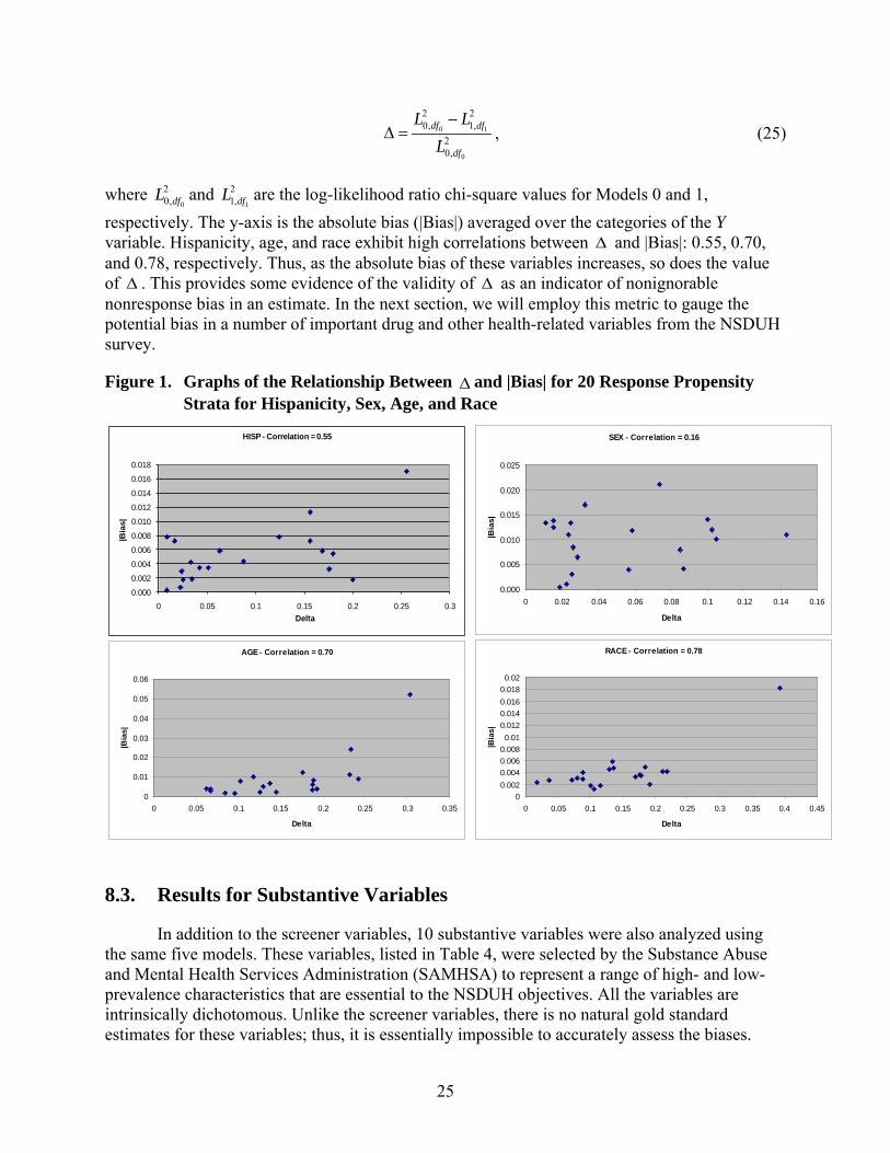
As discussed previously, another use of the callback model is to test for nonignorable nonresponse, for example, by comparing the chi-square values for Models 0 and 1. This test was rejected for all four screener variables and all 20 propensity strata. The graphs in Figure 1 summarize these results for the four screener variables. The x-axis in these graphs is ∆ (delta) defined as

25

0 1

0

2 20, 1,

20,

df df

df

L LL−

∆ = , (25)

where 0

20,dfL and

1

21,dfL are the log-likelihood ratio chi-square values for Models 0 and 1,

respectively. The y-axis is the absolute bias (|Bias|) averaged over the categories of the Y variable. Hispanicity, age, and race exhibit high correlations between ∆ and |Bias|: 0.55, 0.70, and 0.78, respectively. Thus, as the absolute bias of these variables increases, so does the value of ∆ . This provides some evidence of the validity of ∆ as an indicator of nonignorable nonresponse bias in an estimate. In the next section, we will employ this metric to gauge the potential bias in a number of important drug and other health-related variables from the NSDUH survey.

Figure 1. Graphs of the Relationship Between ∆ and |Bias| for 20 Response Propensity Strata for Hispanicity, Sex, Age, and Race

0.000

0.002

0.004

0.006

0.008

0.010

0.012

0.014

0.016

0.018

0 0.05 0.1 0.15 0.2 0.25 0.3

|Bia

s|

Delta

HISP - Correlation = 0.55 SEX - Correlation = 0.16

0.000

0.005

0.010

0.015

0.020

0.025

0 0.02 0.04 0.06 0.08 0.1 0.12 0.14 0.16

Delta

|Bia

s|

AGE - Correlation = 0.70

0

0.01

0.02

0.03

0.04

0.05

0.06

0 0.05 0.1 0.15 0.2 0.25 0.3 0.35

Delta

|Bia

s|

RACE - Correlation = 0.78

00.0020.0040.0060.0080.01

0.0120.0140.0160.0180.02

0 0.05 0.1 0.15 0.2 0.25 0.3 0.35 0.4 0.45

Delta

|Bia

s|

8.3. Results for Substantive Variables

In addition to the screener variables, 10 substantive variables were also analyzed using the same five models. These variables, listed in Table 4, were selected by the Substance Abuse and Mental Health Services Administration (SAMHSA) to represent a range of high- and low- prevalence characteristics that are essential to the NSDUH objectives. All the variables are intrinsically dichotomous. Unlike the screener variables, there is no natural gold standard estimates for these variables; thus, it is essentially impossible to accurately assess the biases.

26

Perhaps the best option for providing some indications of the nonignorable nonresponse bias for these variables is to perform the tests of ignorability by propensity stratum described in Chapter 7.

Following the same approach used for the screener variable analysis, 20 response propensity strata were formed based upon the GEM model. In this analysis, the full GEM model, including the four screener variables was used to form the strata. If the GEM model is successful at removing the bias for a substantive variable, Y, then the tests of ignorability for the variable Y should not be rejected in any stratum. If the test is rejected for one or more strata, then there is at least some evidence that response propensity differs by the levels of Y. This implies that the GEM does not adequately remove the nonignorable nonresponse bias for this Y variable.

An overall measure of the adequacy of the GEM model is the (weighted) average value of ∆ for the 20 response propensity strata, denoted by ∆ , using weights proportional to the stratum size. The larger the value of ∆ , the greater the potential bias in the GEM estimator. To judge the magnitude of ∆ , we can use results for the two dichotomous variables in the screener analysis: sex and Hispanicity. For these variables, ∆ was 0.05 and 0.09, respectively. Both of those variables display an appreciable bias when ∆ exceeded 0.10. This suggests that a ∆ larger than 0.10 might be considered an indication of potentially problematic nonignorable nonresponse bias in the GEM estimator. Of course, this is just a rule of thumb and there is no guarantee that variables for which ∆ is less than 0.10 do not also have large nonignorable nonresponse biases.

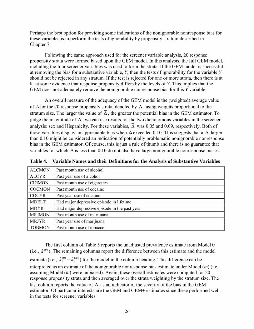
Table 4. Variable Names and their Definitions for the Analysis of Substantive Variables

ALCMON Past month use of alcohol ALCYR Past year use of alcohol CIGMON Past month use of cigarettes COCMON Past month use of cocaine COCYR Past year use of cocaine MDELT Had major depressive episode in lifetime MDYR Had major depressive episode in the past year MRJMON Past month use of marijuana MRJYR Past year use of marijuana TOBMON Past month use of tobacco

The first column of Table 5 reports the unadjusted prevalence estimate from Model 0 (i.e., (0)

1π̂ ). The remaining columns report the difference between this estimate and the model

estimate (i.e., (0) ( )1 1ˆ ˆ mπ π− ) for the model in the column heading. This difference can be

interpreted as an estimate of the nonignorable nonresponse bias estimate under Model (m) (i.e., assuming Model (m) were unbiased). Again, these overall estimates were computed for 20 response propensity strata and then averaged over the strata weighting by the stratum size. The last column reports the value of ∆ as an indicator of the severity of the bias in the GEM estimator. Of particular interests are the GEM and GEM+ estimates since these performed well in the tests for screener variables.

27

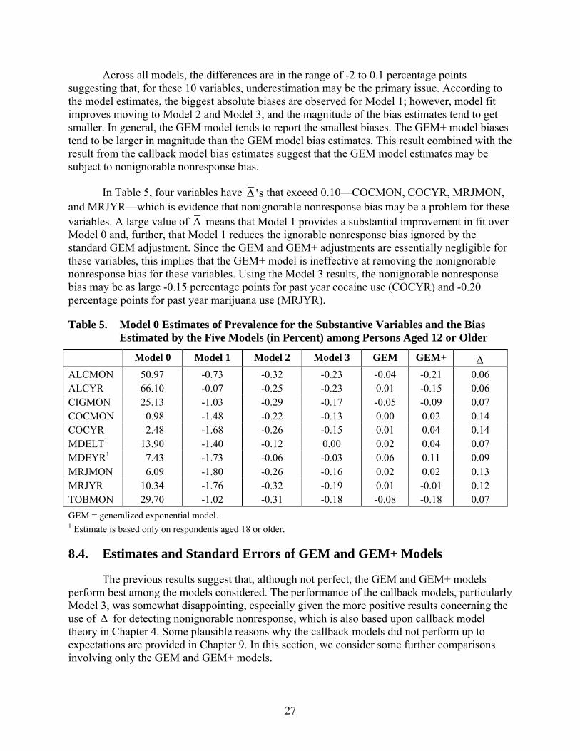
Across all models, the differences are in the range of -2 to 0.1 percentage points suggesting that, for these 10 variables, underestimation may be the primary issue. According to the model estimates, the biggest absolute biases are observed for Model 1; however, model fit improves moving to Model 2 and Model 3, and the magnitude of the bias estimates tend to get smaller. In general, the GEM model tends to report the smallest biases. The GEM+ model biases tend to be larger in magnitude than the GEM model bias estimates. This result combined with the result from the callback model bias estimates suggest that the GEM model estimates may be subject to nonignorable nonresponse bias.

In Table 5, four variables have 's∆ that exceed 0.10—COCMON, COCYR, MRJMON, and MRJYR—which is evidence that nonignorable nonresponse bias may be a problem for these variables. A large value of ∆ means that Model 1 provides a substantial improvement in fit over Model 0 and, further, that Model 1 reduces the ignorable nonresponse bias ignored by the standard GEM adjustment. Since the GEM and GEM+ adjustments are essentially negligible for these variables, this implies that the GEM+ model is ineffective at removing the nonignorable nonresponse bias for these variables. Using the Model 3 results, the nonignorable nonresponse bias may be as large -0.15 percentage points for past year cocaine use (COCYR) and -0.20 percentage points for past year marijuana use (MRJYR).

Table 5. Model 0 Estimates of Prevalence for the Substantive Variables and the Bias Estimated by the Five Models (in Percent) among Persons Aged 12 or Older

Model 0 Model 1 Model 2 Model 3 GEM GEM+ ∆ ALCMON 50.97 -0.73 -0.32 -0.23 -0.04 -0.21 0.06 ALCYR 66.10 -0.07 -0.25 -0.23 0.01 -0.15 0.06 CIGMON 25.13 -1.03 -0.29 -0.17 -0.05 -0.09 0.07 COCMON 0.98 -1.48 -0.22 -0.13 0.00 0.02 0.14 COCYR 2.48 -1.68 -0.26 -0.15 0.01 0.04 0.14 MDELT1 13.90 -1.40 -0.12 0.00 0.02 0.04 0.07 MDEYR1 7.43 -1.73 -0.06 -0.03 0.06 0.11 0.09 MRJMON 6.09 -1.80 -0.26 -0.16 0.02 0.02 0.13 MRJYR 10.34 -1.76 -0.32 -0.19 0.01 -0.01 0.12 TOBMON 29.70 -1.02 -0.31 -0.18 -0.08 -0.18 0.07 GEM = generalized exponential model. 1 Estimate is based only on respondents aged 18 or older.

8.4. Estimates and Standard Errors of GEM and GEM+ Models

The previous results suggest that, although not perfect, the GEM and GEM+ models perform best among the models considered. The performance of the callback models, particularly Model 3, was somewhat disappointing, especially given the more positive results concerning the use of ∆ for detecting nonignorable nonresponse, which is also based upon callback model theory in Chapter 4. Some plausible reasons why the callback models did not perform up to expectations are provided in Chapter 9. In this section, we consider some further comparisons involving only the GEM and GEM+ models.

28

As noted in the screener analysis, the GEM+ model outperformed the GEM model for the more stringent Avg |Bias| Rank criterion suggesting that adding the LOE variable to the GEM could be an improvement over the standard GEM currently in use, particularly for population subgroups analysis (Section 8.2). However, it is still possible that, although the GEM+ model reduces bias, it may increase the standard errors of the estimates. This raises the question of how the mean squared errors (MSEs) of the GEM and GEM+ estimates compare. In addition, any reduction in bias or MSE realized by the GEM+ model may not be sustained throughout the remaining steps of the NSDUH postsurvey adjustment process. As an example, poststratification can also reduce both nonresponse bias and frame coverage bias. It is possible that when poststratification is applied to the GEM and GEM+ model estimates, any MSE reduction afforded by the GEM+ model vanishes.

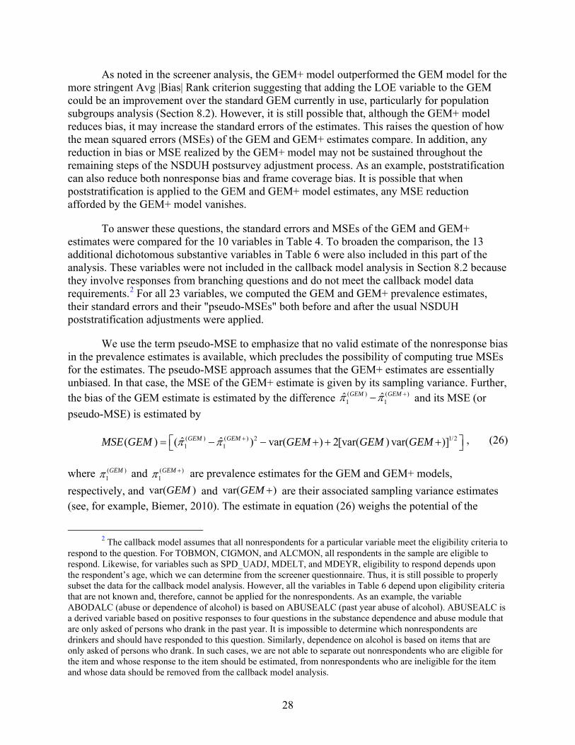
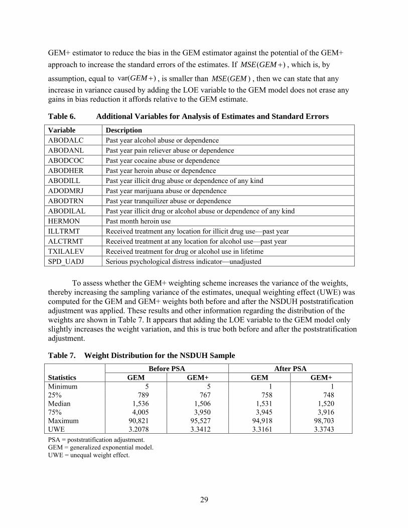
To answer these questions, the standard errors and MSEs of the GEM and GEM+ estimates were compared for the 10 variables in Table 4. To broaden the comparison, the 13 additional dichotomous substantive variables in Table 6 were also included in this part of the analysis. These variables were not included in the callback model analysis in Section 8.2 because they involve responses from branching questions and do not meet the callback model data requirements.2 For all 23 variables, we computed the GEM and GEM+ prevalence estimates, their standard errors and their "pseudo-MSEs" both before and after the usual NSDUH poststratification adjustments were applied.

We use the term pseudo-MSE to emphasize that no valid estimate of the nonresponse bias in the prevalence estimates is available, which precludes the possibility of computing true MSEs for the estimates. The pseudo-MSE approach assumes that the GEM+ estimates are essentially unbiased. In that case, the MSE of the GEM+ estimate is given by its sampling variance. Further, the bias of the GEM estimate is estimated by the difference ( ) ( )

1 1ˆ ˆGEM GEMπ π +− and its MSE (or pseudo-MSE) is estimated by

( ) ( ) 2 1/21 1ˆ ˆ( ) ( ) var( ) 2[var( ) var( )]GEM GEMMSE GEM GEM GEM GEMπ π + = − − + + + , (26)

where ( )1

GEMπ and ( )1

GEMπ + are prevalence estimates for the GEM and GEM+ models, respectively, and var( )GEM and var( )GEM + are their associated sampling variance estimates (see, for example, Biemer, 2010). The estimate in equation (26) weighs the potential of the

2 The callback model assumes that all nonrespondents for a particular variable meet the eligibility criteria to

respond to the question. For TOBMON, CIGMON, and ALCMON, all respondents in the sample are eligible to respond. Likewise, for variables such as SPD_UADJ, MDELT, and MDEYR, eligibility to respond depends upon the respondent’s age, which we can determine from the screener questionnaire. Thus, it is still possible to properly subset the data for the callback model analysis. However, all the variables in Table 6 depend upon eligibility criteria that are not known and, therefore, cannot be applied for the nonrespondents. As an example, the variable ABODALC (abuse or dependence of alcohol) is based on ABUSEALC (past year abuse of alcohol). ABUSEALC is a derived variable based on positive responses to four questions in the substance dependence and abuse module that are only asked of persons who drank in the past year. It is impossible to determine which nonrespondents are drinkers and should have responded to this question. Similarly, dependence on alcohol is based on items that are only asked of persons who drank. In such cases, we are not able to separate out nonrespondents who are eligible for the item and whose response to the item should be estimated, from nonrespondents who are ineligible for the item and whose data should be removed from the callback model analysis.

29

GEM+ estimator to reduce the bias in the GEM estimator against the potential of the GEM+ approach to increase the standard errors of the estimates. If ( )MSE GEM + , which is, by

assumption, equal to var( )GEM + , is smaller than ( )MSE GEM , then we can state that any increase in variance caused by adding the LOE variable to the GEM model does not erase any gains in bias reduction it affords relative to the GEM estimate.

Table 6. Additional Variables for Analysis of Estimates and Standard Errors

Variable Description ABODALC Past year alcohol abuse or dependence ABODANL Past year pain reliever abuse or dependence ABODCOC Past year cocaine abuse or dependence ABODHER Past year heroin abuse or dependence ABODILL Past year illicit drug abuse or dependence of any kind ADODMRJ Past year marijuana abuse or dependence ABODTRN Past year tranquilizer abuse or dependence ABODILAL Past year illicit drug or alcohol abuse or dependence of any kind HERMON Past month heroin use ILLTRMT Received treatment any location for illicit drug use—past year ALCTRMT Received treatment at any location for alcohol use—past year TXILALEV Received treatment for drug or alcohol use in lifetime SPD_UADJ Serious psychological distress indicator—unadjusted

To assess whether the GEM+ weighting scheme increases the variance of the weights, thereby increasing the sampling variance of the estimates, unequal weighting effect (UWE) was computed for the GEM and GEM+ weights both before and after the NSDUH poststratification adjustment was applied. These results and other information regarding the distribution of the weights are shown in Table 7. It appears that adding the LOE variable to the GEM model only slightly increases the weight variation, and this is true both before and after the poststratification adjustment.

Table 7. Weight Distribution for the NSDUH Sample

Statistics Before PSA After PSA

GEM GEM+ GEM GEM+ Minimum 5 5 1 1 25% 789 767 758 748 Median 1,536 1,506 1,531 1,520 75% 4,005 3,950 3,945 3,916 Maximum 90,821 95,527 94,918 98,703 UWE 3.2078 3.3412 3.3161 3.3743 PSA = poststratification adjustment. GEM = generalized exponential model. UWE = unequal weight effect.

30

Next, prevalence estimates and their associated standard errors and MSEs were computed using these weights, and these results are shown in Table 8. There are no discernible patterns in the direction of differences in estimates and standard errors between the GEM and GEM+ model before or after the poststratification adjustment. In Table 8, more than half (16 out of 23) of the estimates from GEM+ model had smaller MSE than the estimates from GEM model before the PSA, and 18 out of 23 estimates from GEM+ model had smaller MSE than the estimates from GEM model after the poststratification adjustment. These results suggest that adding LOE in the nonresponse adjustment model could improve estimates.

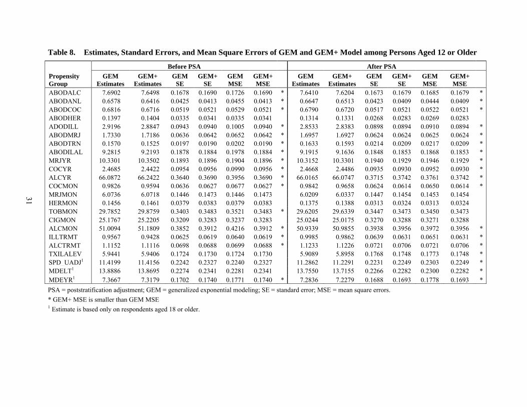
31

Table 8. Estimates, Standard Errors, and Mean Square Errors of GEM and GEM+ Model among Persons Aged 12 or Older

Propensity Group

Before PSA After PSA GEM

Estimates GEM+

Estimates GEM

SE GEM+

SE GEM MSE

GEM+ MSE

GEM Estimates

GEM+ Estimates

GEM SE

GEM+ SE

GEM MSE

GEM+ MSE

ABODALC 7.6902 7.6498 0.1678 0.1690 0.1726 0.1690 * 7.6410 7.6204 0.1673 0.1679 0.1685 0.1679 * ABODANL 0.6578 0.6416 0.0425 0.0413 0.0455 0.0413 * 0.6647 0.6513 0.0423 0.0409 0.0444 0.0409 * ABODCOC 0.6816 0.6716 0.0519 0.0521 0.0529 0.0521 * 0.6790 0.6720 0.0517 0.0521 0.0522 0.0521 * ABODHER 0.1397 0.1404 0.0335 0.0341 0.0335 0.0341 0.1314 0.1331 0.0268 0.0283 0.0269 0.0283 ADODILL 2.9196 2.8847 0.0943 0.0940 0.1005 0.0940 * 2.8533 2.8383 0.0898 0.0894 0.0910 0.0894 * ABODMRJ 1.7330 1.7186 0.0636 0.0642 0.0652 0.0642 * 1.6957 1.6927 0.0624 0.0624 0.0625 0.0624 * ABODTRN 0.1570 0.1525 0.0197 0.0190 0.0202 0.0190 * 0.1633 0.1593 0.0214 0.0209 0.0217 0.0209 * ABODILAL 9.2815 9.2193 0.1878 0.1884 0.1978 0.1884 * 9.1915 9.1636 0.1848 0.1853 0.1868 0.1853 * MRJYR 10.3301 10.3502 0.1893 0.1896 0.1904 0.1896 * 10.3152 10.3301 0.1940 0.1929 0.1946 0.1929 * COCYR 2.4685 2.4422 0.0954 0.0956 0.0990 0.0956 * 2.4668 2.4486 0.0935 0.0930 0.0952 0.0930 * ALCYR 66.0872 66.2422 0.3640 0.3690 0.3956 0.3690 * 66.0165 66.0747 0.3715 0.3742 0.3761 0.3742 * COCMON 0.9826 0.9594 0.0636 0.0627 0.0677 0.0627 * 0.9842 0.9658 0.0624 0.0614 0.0650 0.0614 * MRJMON 6.0736 6.0718 0.1446 0.1473 0.1446 0.1473 6.0209 6.0337 0.1447 0.1454 0.1453 0.1454 HERMON 0.1456 0.1461 0.0379 0.0383 0.0379 0.0383 0.1375 0.1388 0.0313 0.0324 0.0313 0.0324 TOBMON 29.7852 29.8759 0.3403 0.3483 0.3521 0.3483 * 29.6205 29.6339 0.3447 0.3473 0.3450 0.3473 CIGMON 25.1767 25.2205 0.3209 0.3283 0.3237 0.3283 25.0244 25.0175 0.3270 0.3288 0.3271 0.3288 ALCMON 51.0094 51.1809 0.3852 0.3912 0.4216 0.3912 * 50.9339 50.9855 0.3938 0.3956 0.3972 0.3956 * ILLTRMT 0.9567 0.9428 0.0625 0.0619 0.0640 0.0619 * 0.9985 0.9862 0.0639 0.0631 0.0651 0.0631 * ALCTRMT 1.1152 1.1116 0.0698 0.0688 0.0699 0.0688 * 1.1233 1.1226 0.0721 0.0706 0.0721 0.0706 * TXILALEV 5.9441 5.9406 0.1724 0.1730 0.1724 0.1730 5.9089 5.8958 0.1768 0.1748 0.1773 0.1748 * SPD_UADJ1 11.4199 11.4156 0.2242 0.2327 0.2240 0.2327 11.2862 11.2291 0.2231 0.2249 0.2303 0.2249 * MDELT1 13.8886 13.8695 0.2274 0.2341 0.2281 0.2341 13.7550 13.7155 0.2266 0.2282 0.2300 0.2282 * MDEYR1 7.3667 7.3179 0.1702 0.1740 0.1771 0.1740 * 7.2836 7.2279 0.1688 0.1693 0.1778 0.1693 * PSA = poststratification adjustment; GEM = generalized exponential modeling; SE = standard error; MSE = mean square errors. * GEM+ MSE is smaller than GEM MSE 1 Estimate is based only on respondents aged 18 or older.

32

This page intentionally left blank.

33

9. The Quality of the NSDUH Callback Data There are several possible explanations for why the callback model estimates considered

in Sections 8.1 and 8.2 showed little or no improvement over the GEM and GEM+ model estimates. Obviously, these results suggest that the callback models are misspecified in some way because a well-specified model should produce better results. Based upon the experience from this application, we believe the problem does not stem from the lack of fit of the models. For example, adding more α parameters to the model, while improving model fit, did not reduce the bias in the estimates of prevalence. In fact, an interesting phenomenon was observed regarding the β parameters. Models that allowed the β parameters to vary across the levels of Y markedly improved the model fit, yet the resulting prevalence estimates were substantially more biased. One possibility for these puzzling results is that data that are being used to model response propensity in the callback models (i.e., the callback data) are flawed for the purpose of callback modeling.

The callback model assumes that the number call attempts are recorded accurately by the interviewers. The estimated response propensity for an individual is a function of the number of callbacks that were made on behalf of that individual to obtain an initial contact. Even small errors in the number of callbacks can cause biases in the estimates of response propensity. As a result, the nonresponse weighting adjustments, which are functions of the estimated response propensities, will be biased resulting in either overcorrecting or undercorrecting the weights.

To see this, consider the simple expression for response propensity in equation (6) and suppose 0.2α = for all sample persons. If the number of callbacks is actually K = 3, the estimated response propensity by this formula is estimated to be 0.49. If instead the interviewer records only K=2 call attempts for this case, the estimated response propensity drops to 0.36. Likewise, if the interviewer records K=4 attempts rather than 3, the estimated response propensity increases to 0.59. Such recording errors can make a meaningful difference in the weight that is applied to a case. For example, instead of a weight factor of around 2.0 (with K=3), a weight factor of 2.8 (K=2) or 1.7 (K=4) would be applied.

A small level of error in the callback data is unavoidable and, based upon preliminary results from a limited simulation study, will not create important biases in the callback model estimates. The effect of measurement error will be larger when there are fewer callbacks than when there are a greater number of callbacks. In other words, the error associated in recording two or four callbacks when three should have been recorded is much larger than in recording 12 or 14 callbacks when 13 should have been recorded. In the present analysis, the number of callbacks was truncated at 15, and all cases not finalized at that call attempt were treated as censored. This appeared to have no appreciable effects on the estimates. Future applications might consider lowering the truncation limit to 12 or even 10 to ameliorate callback error bias for higher numbers of callbacks.

It would seem that any response propensity model incorporating level of effort (LOE) would be subject to this callback error bias. Interestingly, however, the GEM+ appears to be less

34

susceptible, which may account for its apparent superior performance in this study. The GEM+ model may be more robust to these errors because it uses the sum total of all call attempts to contact a case in the model rather than the outcomes from each individual attempt as the callback models do. In addition, there are 13 other variables in the GEM+ model that reduces the effects of an error in any one variable. Still, we believe the performance of any response propensity model that incorporates LOE data would be improved if the LOE data could be obtained accurately.

Because the quality of the callback data is an important question for this research, this question was addressed to some extent in this study by investigating the process used to collect the callback data. The purpose of this investigation was twofold. First, we wanted to learn about the accuracy of the callback data regarding the needs of the callback model. In particular, we sought information from field staff on how callback data are recorded and what factors might lead interviewers to record information on callbacks incorrectly. Second, we wished to obtain recommendations from the field staff for either improving the accuracy of entering callback data or making the process easier to carry out without reducing the accuracy or imposing additional burdens on the field staff. First, an informal survey was conducted in September 2009 of all National Survey on Drug Use and Health (NSDUH) interviewers that asked about their current reporting practices and how they would handle specific situations in the field. A total of 601 responses were obtained from 653 interviewers.

A typical sample question from this survey is the following:

You approach a controlled access community containing several dwelling units. While trying to enter, you are stopped by a security guard and after speaking with him briefly, he refuses to let you enter. Later in the day, you make a second visit and notice the same security guard standing outside. You do not attempt to speak to him again and decide to work in another part of the segment. Would you enter a record to document this second visit to the community in control system?

In addition to the survey, two teleconference meetings were conducted with groups of field supervisors, regional supervisors, and regional directors during the same period.

A full report of the findings from this investigation appears in Appendix A. However, the following bullet points summarize the main findings.

• Underreporting seems to be more frequent than overreporting of call attempts.

– Interviewers are prevented from overreporting because this practice can usually be discovered through timesheet reviews, and the consequences of intentionally falsifying these data are severe.

– Underreporting may occur because of pressures to keep a case "alive." If too many unproductive visits are recorded, the case may get closed out.

– Field staff wishing to avoid being perceived as not using time effectively may also underreport.

– Failure to report "drive-by" visits seems to be a primary cause of underreporting.

35

– Another frequent cause of underreporting is the failure to report attempts to interview multiple sample persons within the same household.

• The degree of underreporting can vary a lot by interviewer. This interviewer variance is very difficult to model in any nonresponse adjustment framework.

• Depending on the level of precision needed for callback modeling, potential changes range from modest (e.g., interviewer prompts when there are two interviews in a household) to extensive (e.g., new definitions of visits and procedures for recording visits).

This study concluded that the level of error in the callback data for callback modeling purposes is quite high and has the potential to seriously bias the results of the callback modeling approach to nonresponse adjustment. Our limited simulation study confirmed that even a small degree of underreporting (say 5 percent) is enough to appreciably bias the callback model estimates. But add to this the complications introduced by variations among supervisors, interviewers, and types of units in the levels of underreporting and the situation becomes somewhat intractable to address through model enhancements alone. Rather, the preferred solution would seem to be improvements in the quality of the callback data for modeling purposes at its source. Unfortunately, changing the field procedures currently in use for collecting these data and introducing additional quality checks to ensure accurate reporting of callbacks suitable for callback modeling would introduce additional burdens on interviewers. One concern is that increasing the burden associated with this task could draw the interviewer's attention away from crucial tasks such as contacting sample members, gaining their cooperation, and conducting the interview. A more prudent approach would be to wait until the NSDUH field systems are redesigned to take advantage of new technologies and other innovations. At that opportunity, a common purpose of the callback data for accuracy and other paradata should be considered a high priority.

36

This page intentionally left blank.

37

10. Conclusions The number of callbacks required to establish contact with a sample person is strongly

correlated with that person's contactability. Two basic approaches for incorporating this information into the nonresponse adjustment process were investigated in this study. One approach, the callback model, essentially equates a person's response propensity to the product of the probability of contact at each attempt and the probability of an interview given an initial contact was made. The second approach (referred to as GEM+) incorporates a level of effort (LOE) variable in a traditional logistic regression model for response propensity. Both approaches were compared with the current logistic regression approach (referred to as GEM) used in the National Survey on Drug Use and Health (NSDUH). The nonignorable nonresponse biases in four screener variables and 10 substantive variables were estimated for the null model (Model 0), three callback models, the GEM+ model, and the GEM model. The mean square errors (MSEs) of the GEM and GEM+ models were compared further for 13 additional substantive variables.

A basic framework for investigating these models was developed that incorporated 20 response propensity strata. For each screener variable (sex, ethnicity, age, and race), the strata were created using the GEM model estimates of response propensities. However, to simulate nonignorable nonresponse, the screener variable was left out of the GEM model. The ability of the various models to compensate for the "ignored" variable was then assessed at the stratum level and overall. For the substantive variables, the full GEM model was used to create the response propensity strata. The variation in the estimates across the models was assessed both at the stratum level and overall.

In addition to developing the basic framework for estimating and comparing these models, the study also developed a new statistic for gauging the severity of nonignorable nonresponse bias based upon a test of ignorability. This statistic, denoted by ∆ , was moderately to highly correlated with nonignorable nonresponse bias in the screener variables that were analyzed. It was used in the analysis of the substantive variables to identify variables that are most susceptible to nonignorable nonresponse bias under the GEM model.

The study confirmed what we know from other studies on nonresponse adjustment approaches (i.e., there is no uniformly best approach for reducing the effects of nonresponse on survey estimates). In our study, all models—even the null model—were the best in some situations. However, in our most stringent test, the GEM+ model ranked best overall in removing nonignorable nonresponse bias for the screener variables—the only variables were this bias could be estimated. The current GEM model ranked a close second. The best callback model, Model 3, did not outperform either of the regression models.

In our analysis, improving model fit did not always improve model performance. In fact, specifying more complex models actually increased model bias in some cases even while model fit significantly improved. These results suggest that the lackluster performance of the callback modeling approach in this study is attributable to callback data errors. Bolstering this view, an informal investigation of the process for collecting LOE data suggests that the underreporting errors in the NSDUH record of calls (ROCs) data is substantial and may be problematic for

38

applications requiring a high degree of accuracy in these data like callback modeling. A limited simulation study (not discussed in this report) confirmed that even a small level of underreporting error (say 5 percent) can cause appreciable biases in the callback model estimates.

It may be possible to somehow incorporate an error term in the callback modeling approach to correct for underreporting error; however, given the potential complexity of these errors, modeling them is ostensibly not a viable option. A more successful approach may be to introduce changes in the data collection process to enhance the quality of the callback data. However, because of the likely burdens they would impose on the interviewers, such changes will have to wait until a complete redesign of the field systems can be mounted.

Biemer and Link (2007) report much better success with the callback modeling approach in their application to the Behavior Risk Factor Surveillance System (BRFSS)—a national random-digit dialing (RDD) survey. However, callback data could be of much greater quality in this survey, as well as in RDD surveys in general, because of the controls in place for recording call attempts and their outcomes for each dialed number. In addition, in their study, the callback model was competing with a somewhat ineffective poststratification adjustment approach for adjusting for nonresponse bias in the BRFSS. In that situation, the callback model provided a marked improvement in bias reduction. By contrast, the NSDUH GEM model uses a considerable amount of data available at the household level. It should be no surprise then that adding an LOE variable to this extensive amount of data showed much less improvement.

39

References Alho, J. (1990). Adjusting for nonresponse bias using logistic regression. Biometrika, 77(3), 617-624.

Anido, C., & Valdés, T. (2000). An iterative estimating procedures for probit-type nonresponse models in surveys with call backs. Sociedad de Estadística e Investigación Operativa Test, 9(1), 233-253.

Biemer, P. (2010). Overview of design issues: Total survey error. In Marsden, P. & Wright, J. (Eds.), Handbook of survey research, Second Edition. Emerald Group Publishing, LTD, Bingley, UK

Biemer, P., & Christ, S. (2008). Weighting survey data. In Hox, J., E. De Leeuw, & D. Dillman (Eds.), International handbook of survey methodology. Mahwah, NJ: Lawrence Erlbaum Associates.

Biemer, P., & Link, M. (2007). Evaluating and modeling early cooperator bias in RDD surveys. In Lepkowski, J. et al. (Eds.), Advances in telephone survey methodology. Hoboken, NJ: John Wiley & Sons.

Biemer, P., & Wang, K. (2007). Using callback models to adjust for nonignorable nonresponse in face-to-face surveys. Proceedings of the 2007 Joint Statistical Meetings, American Statistical Association, Section on Survey Research Methods, Salt Lake City, UT.

Brick, J. M., & Kalton, G. (1996). Handling missing data in survey research. Statistical Methods in Medical Research, 5, 215-238.

Chen, P., Dai, L., Gordek, H., Shi, W., Singh, A., & Westlake, M. (2005). Person-level sampling weight calibration for the 2003 NSDUH. In 2003 National Survey on Drug Use and Health: Methodological resource book (Section 3, prepared for the Substance Abuse and Mental Health Services Administration, Office of Applied Studies, under Contract No. 283-98-9008, Deliverable No. 28, RTI/07190.574.100). Research Triangle Park, NC: RTI International.

Dempster, A. P., Laird, N. M., & Rubin, D. B. (1977). Maximum likelihood from incomplete data via the EM algorithm. Journal of the Royal Statistical Society, B, 1-38.

Drew, J. H., & Fuller, W. A. (1980). Modeling nonresponse in surveys with callbacks. Proceedings of the Survey Research Methods Section, American Statistical Association, pp. 639-42. Washington, DC: American Statistical Association.

Folsom, R. E., & Singh, A. C. (2000). The generalized exponential model for sampling weight calibration for extreme values, nonresponse, and poststratification. Proceedings of the 2000 Joint Statistical Meetings, American Statistical Association, Survey Research Methods Section, Indianapolis, IN.

40

Groves, R. M., & Couper, M. P. (1998). Nonresponse in household interview surveys. New York: John Wiley.

Hartley, H. O. (1946). Discussion on A review of recent statistical developments in sampling and sampling surveys by F. Yates. Journal of the Royal Statistical Society A, 109, 37-38.

Lessler, J. & Kalsbeek, W. (1992). Nonsampling errors in surveys. New York: John Wiley.

Little, R. J. A. (1986). Survey nonresponse adjustments for estimates of means. International Statistical Review, 54(2), 139-157.

Little, R. J. A., & Rubin, D. B. (1987). Statistical analysis with missing data. New York: John Wiley.

Politz, A., & Simmons, W. (1949). An attempt to get the ‘not at homes’ into the sample without callbacks. Journal of the American Statistical Association, 44(245), 9-16.

Potthoff, R. F., Manton, K. G., & Woodbury, M. A. (1993). Correcting for nonavailability bias in surveys by weighting based on number of callbacks. Journal of the American Statistical Association, 88(424), 1197-1207.

Vartivarian, S., & Little, R. (2003). On the formation of weighting adjustment cells for unit nonresponse. The University of Michigan Department of Biostatistics Working Paper Series. Working Paper 10.

Wood, A. W., White, I. R., & Hotopf, M. (2006). Using number of failed contact attempts adjust for non-ignorable non-response. Journal of the Royal Statistical Association, A, 169(3), 525-542.

A-1

Appendix A: Investigation of Call Record Data Properties

The callback model assumes that all visits to potential respondents are recorded and that a visit can be defined and recorded in a standard way. The estimated response propensity for an individual case is a function of the number of callbacks. If the number of callbacks is not recorded accurately, the response propensity will be estimated incorrectly. In turn, nonresponse weighting adjustments are a function of the estimated response propensity. Thus, errors in recording the number of callbacks will result in nonresponse weighting adjustments that are too large or too small. In general, as the number of callbacks increases, the response propensity increases and the nonresponse adjustment factor decreases. If too many callbacks are recorded relative to the true number of callbacks, the response propensity will be underestimated and the resulting weight adjustment will be too large. If too few callbacks are recorded, the response propensity will be underestimated and the associated weight adjustment will seem too small. Also, the impact of measurement error will be larger when there are fewer callbacks than when there are a greater numbers of callbacks. In other words, the error associated in recording two or four callbacks when three should have been recorded is much larger than in recording 12 or 14 callbacks when 13 should have been recorded.

The purpose of this investigation was twofold. First, we wished to learn about the accuracy of the callback data in terms of recording actual visits to sample dwelling units. In particular, we sought information from field staff on how callback data are recorded and what factors might lead field interviewers (FIs) to record information on callbacks in ways that differ from how callbacks are conceptualized in the callback model. Second, we wished to obtain recommendations from the field staff for either improving the accuracy of entering callback data or making the process easier to carry out without reducing the accuracy or imposing additional burdens on the field staff.

Description of the Investigation

We used two methods to obtain information from field staff on the suitability of the callback data. First, we administered an informal questionnaire to FIs in which we asked interviewers several questions about their practices in recording callback data. In several questions, interviewers were presented with hypothetical scenarios and asked what, if anything, they would enter into the callback data. Overall, 601 out of 653 (92 percent) of interviewers completed the questionnaire between September 8, 2009 and September 16, 2009.

Second, we conducted two conference calls with groups of field supervisors and regional supervisors, along with the regional directors. The calls were held on September 29, 2009 and October 5, 2009. The calls involved a total of 10 field supervisors and six regional supervisors. In addition, all three regional directors participated in both calls. Other attendees included the NSDUH operations director, national field director, and project director. In these calls, we asked supervisors about their experiences with reasons for over- or underreporting of visits in the

A-2

record of calls (ROC) data, practices for reviewing the entry of visits in the ROC data, and about problems, complaints, or questions they receive from interviewers about the ROC system.

Findings

One conclusion from the conference calls was that supervisors believed that underreporting of visits was more prevalent than overreporting. Supervisors noted two reasons that FIs might have an incentive to underreport visits. First, there may be underreporting of visits if FIs are concerned that project management staff will instruct supervisors to close out cases that have a high number of ROC entries. The number of ROCs along with other information at the case level is used to define viable cases. In addition, FIs may underreport visits if they are concerned about appearing inefficient in using their time.

Supervisors felt that "padding" or overreporting of visits was much less prevalent than underreporting. An FI might be motivated to overreport visits if they want their supervisor to think they were working when they were not. FIs are instructed to work in a segment for at least 4 hours each day when they are in the segment, so an FI may overreport visits if they want to make it appear they are fulfilling the work requirement. Also, in the third month of the quarter, when many cases have closed out and there is comparatively less work available, an FI may overreport visits to keep their pay consistent throughout the quarter. Supervisors can detect both underreporting and overreporting by comparing FI timesheets and ROC entries. FIs that are detected "padding" are caught quickly through timesheet reviews and removed from the project.

A major source of error in reporting visits stems from the treatment of "drive-bys" or situations in which an interviewer goes to the dwelling unit and for whatever reason does not knock on the door or otherwise attempt to contact the dwelling unit.

• In some cases, the interviewer may be relying upon visual cues to determine if anything about the dwelling unit has changed to indicate that someone is in the unit. For example, an FI may check on a dwelling unit after an initial visit in which no one was home. If there is no visible change in the unit (e.g., no car nearby), the FI may conclude that no one is home and not record this as a visit.

• In more extreme cases, supervisors cited examples in which a person in the household was selected for the interview but the screener respondent gave a specific cue for the interviewer to look for to see if the selected person was home and not bother knocking in the absence of that cue. For example, the screener respondent may say that the selected person drives a particular vehicle and the FI should knock on the door only if that vehicle is at the dwelling unit.

• Supervisors reported that some FIs will drive-by dwelling units if they just happen to be in the area but will not record these visits since they are going by on their own time.

All these cases should be recorded as visits. When they are not it results in underreporting. To an interviewer, such visits may not seem very informative for the purpose of case management and therefore not worth entering in the ROC data. However, from the

A-3

perspective of estimating response propensity, such visits are worth noting since they are predictive of response propensity.

In responses to the survey administered to interviewers, there were expressions of uncertainty about how to treat drive-bys because of potentially conflicting instructions or motivations to keep ROC entries down. One key factor determining if an entry is made in the ROC data is whether the FI attempted to make contact. We asked the following question in our survey of FIs:

You approach a controlled access community containing several SDUs. While trying to enter the community, you are stopped by a security guard and after speaking with him briefly, he refuses to let you enter. Later in the day, you make a second visit to the community and notice the same security guard standing outside. You do not attempt to speak to him again and decide to work in another part of the segment.

Would you enter a ROC to document this second visit to the community in your iPAQ?

Half of the FIs were asked this question. The other half of the sample was asked the same question except that a different guard appears in the second visit and this guard also refuses to grant entry. In the first version, 79 percent of FIs responded that they would record the second visit in the ROC data. In the second version, 99 percent of FIs responded that they would record the second visit. Thus, for 20 percent of FIs, whether an attempt is made determines if the visit is recorded.

Finally, drive-bys may be underreported when FIs resort to summarizing a number of different attempts within a single ROC entry. Thus, what appears to be one visit actually represents several visits during the same day. The FI may or may not note this in the open-ended text. This is particularly likely to occur toward the end of the quarter when an FI may make several visits to the unit in a last-ditch effort to obtain a completed interview.

Another source of underreporting stems from cases where many attempts have been made and nearing the end of the field period, a field supervisor may instruct the FI to make one last visit. If they are unsuccessful in obtaining a completed screener or interview, the FI closes the case out and assigns it a final result code. We asked FIs a question about such "one and done" situations as follows:

Your FS has instructed you to make one last attempt to contact an interview respondent who you've never been able to find at home, and has given you permission to final code the case if you are not able to complete the interview today. You go to the SDU and no one is home.

Which interview result code(s) would you enter for this case?

In this situation, FIs should make two ROC entries. The first would be an interim one indicating that no one was home and the second one would be final result code (no one home after repeated visits). But 44 percent of FIs answered that they would only enter a single ROC

A-4

entry, the final result code. Thus, for situations like this, the number of visits would be underreported. Also, the current system for entering information on visits does not allow for FIs to indicate if they are operating under such one and done instructions, so the scope of the underreporting is unknown.

Not all errors are associated with over- or underreporting. That the NSDUH interviews up to two persons in eligible dwelling units can also contribute to errors in reporting the numbers of visits. During each visit to a dwelling unit with two persons selected for an interview, FIs should normally record visits for each selected person (unless separate appointments have been made at different times). In some cases, FIs will forget to record visits for both selected persons, leading to underreporting of visits. FIs may also introduce error in either the numbers of visits or the result codes for those visits by recording information for the first selected respondent in the call history for the second selected respondent and vice versa. In response to a survey question about this, 17 percent of FIs responded that they have switched around ROC entries for different respondents in the same dwelling unit either "often" or "sometimes."

Conclusion

Overall, we found more evidence of underreporting of visits in NSDUH ROC data than overreporting. If interviewers underreport visits, response propensities will be underestimated, but if the underreporting is consistent across interviewers and over time, adjustments could be made to the callback models.

However, underreporting appears to be driven by a set of factors that can vary by interviewer. Some interviewers will record all drive-bys as separate ROC entries, some will collapse multiple drive-bys into a single ROC, and some will not enter drive-bys as ROC entries. Individual interviewers will also have different levels of concern about reporting too many drive-bys and appearing to be inefficient or have different levels of concern about having cases closed out due to reporting too many visits. Finally, we saw differences in interviewer responses in what they would enter in the ROC data under hypothetical scenarios. Thus, interviewer variability in recording visits needs to be accounted for in modeling response propensities, which may make the models intractable.

The NSDUH system for recording visits serves primarily as a means for interviewers and supervisors to help manage caseloads. Changes in the system or the development of another system would be needed to obtain more accurate data on visits for the purpose of callback models. Some of the changes could be fairly modest. For example, for households with two persons selected for the interview, a pop-up reminder could make the interviewer aware to enter an ROC for the second case (if necessary) after the FI has entered one for the first case. Other changes would be more difficult to implement and potentially costly. For example, having interviewers enter all visits in the ROC data, perhaps by including a result code for drive-bys, could require modifications to the iPAQ program and reporting systems, additional or modified training for interviewers and supervisors, and an additional burden to interviewers in terms of the time required to enter the additional visits. Extensive changes in the collection of call record data could also adversely affect the main data collection effort that the ROC data supports.