implicit abstraction heuristics for cost-optimal planning · 4.11 miconic: causal graph and the...
TRANSCRIPT

Implicit Abstraction Heuristics for Cost-Optimal Planning
Michael Katz

Implicit Abstraction Heuristics for Cost-Optimal Planning
Research Thesis
In Partial Fulfillment of the
Requirements for the
Degree of Doctor of Philosophy
Michael KatzSubmitted to the Senate of
the Technion - Israel Institute of Technology
Av, 5770 Haifa August 2010

2

The Research Thesis Was Done Under The Supervision of Prof. Carmel Domshlak in theFaculty of Industrial Engineering and Management.
First of all, I would like to express my sincere gratitude to Prof. Carmel Domshlak, who hasbeen my supervisor since the beginning of my study. He was not only the best supervisor one couldpossibly dream of, but also a great personal friend. I would also like to thank Erez Karpas foruncountable helpful discussions.
The Generous Financial Help Of Technion Is Gratefully Acknowledged.
Last, but not least, I would like to thank my family and friends, who supported me over theyears. I could not do it without you.
I

II
Contents
1 Introduction 1
2 Classical Planning, Heuristic Search, and Abstractions 92.1 Planning Tasks and Abstractions . . . . . . . . . . . . . . . . . . . . . . . . . . . . . 92.2 Heuristic Functions and Abstractions . . . . . . . . . . . . . . . . . . . . . . . . . . . 14
2.2.1 Admissible Heuristics and Heuristic Ensembles . . . . . . . . . . . . . . . . . 142.2.2 Abstraction Heuristics . . . . . . . . . . . . . . . . . . . . . . . . . . . . . . . 152.2.3 Explicit Abstractions . . . . . . . . . . . . . . . . . . . . . . . . . . . . . . . . 15
3 Tractable Fragments of Cost-Optimal Planning 173.1 Binary Variable Domains . . . . . . . . . . . . . . . . . . . . . . . . . . . . . . . . . 20
3.1.1 Cost-optimal planning for Pb . . . . . . . . . . . . . . . . . . . . . . . . . . . 213.1.2 Cost-optimal planning for P(1) . . . . . . . . . . . . . . . . . . . . . . . . . . 213.1.3 Drawing the Limits of k-dependence . . . . . . . . . . . . . . . . . . . . . . . 233.1.4 Towards Practically Efficient Special Cases . . . . . . . . . . . . . . . . . . . 25
3.2 General Variable Domains . . . . . . . . . . . . . . . . . . . . . . . . . . . . . . . . . 273.2.1 Cost-optimal planning for F . . . . . . . . . . . . . . . . . . . . . . . . . . . . 273.2.2 Cost-optimal planning for IF . . . . . . . . . . . . . . . . . . . . . . . . . . . 30
4 Implicit Abstractions 334.1 Implicit Abstractions: Basic Idea . . . . . . . . . . . . . . . . . . . . . . . . . . . . . 344.2 Acyclic Causal-Graph Decompositions . . . . . . . . . . . . . . . . . . . . . . . . . . 364.3 Fork Decomposition . . . . . . . . . . . . . . . . . . . . . . . . . . . . . . . . . . . . 394.4 Accuracy of Fork-Decomposition Heuristics . . . . . . . . . . . . . . . . . . . . . . . 46
4.4.1 Asymptotic Performance Analysis . . . . . . . . . . . . . . . . . . . . . . . . 464.4.2 Experimental Evaluation . . . . . . . . . . . . . . . . . . . . . . . . . . . . . 68
4.5 Back to Theory: h-Partitions and Databased Implicit Abstractions . . . . . . . . . . 704.5.1 Fork Databases . . . . . . . . . . . . . . . . . . . . . . . . . . . . . . . . . . . 714.5.2 Inverted Fork Databases . . . . . . . . . . . . . . . . . . . . . . . . . . . . . . 734.5.3 Experimental Evaluation . . . . . . . . . . . . . . . . . . . . . . . . . . . . . 76
5 Abstraction-based Heuristics Composition 795.1 LP-Optimizable Ensembles of Abstractions . . . . . . . . . . . . . . . . . . . . . . . 835.2 LP-Optimization and Explicit Abstractions . . . . . . . . . . . . . . . . . . . . . . . 855.3 LP-Optimization and Implicit Abstractions I: Fork Decomposition . . . . . . . . . . 875.4 LP-Optimization and Implicit Abstractions II: Tree-structured COPs . . . . . . . . . 94
III
5.5 Experimental Evaluation . . . . . . . . . . . . . . . . . . . . . . . . . . . . . . . . . . 985.6 Beyond Optimal Cost Partitioning . . . . . . . . . . . . . . . . . . . . . . . . . . . . 100
6 Summary and Future Work 103
Bibliography 107
A Compexity Results in Detail 113A.1 Cost-Optimal Planning for Pb . . . . . . . . . . . . . . . . . . . . . . . . . . . . . . . 113
A.1.1 Construction . . . . . . . . . . . . . . . . . . . . . . . . . . . . . . . . . . . . 113A.1.2 Correctness and Complexity . . . . . . . . . . . . . . . . . . . . . . . . . . . . 117
A.2 Cost-Optimal Planning for P(1) with Uniform-Cost Actions . . . . . . . . . . . . . . 123A.2.1 Post-Unique Plans and P(1) Problems . . . . . . . . . . . . . . . . . . . . . . 123A.2.2 Construction . . . . . . . . . . . . . . . . . . . . . . . . . . . . . . . . . . . . 126A.2.3 Correctness and Complexity . . . . . . . . . . . . . . . . . . . . . . . . . . . . 129
A.3 Cost-Optimal Planning for P(1) with General Action Costs . . . . . . . . . . . . . . 135A.3.1 Post-3/2 Plans and P(1) Problems . . . . . . . . . . . . . . . . . . . . . . . . 136A.3.2 Construction . . . . . . . . . . . . . . . . . . . . . . . . . . . . . . . . . . . . 158A.3.3 Correctness and Complexity . . . . . . . . . . . . . . . . . . . . . . . . . . . . 168
B Experimental Evaluation in Detail 177B.1 Fork-Decompositon . . . . . . . . . . . . . . . . . . . . . . . . . . . . . . . . . . . . . 177B.2 Databased Fork-Decompositon . . . . . . . . . . . . . . . . . . . . . . . . . . . . . . 183B.3 Optimal Cost Partition . . . . . . . . . . . . . . . . . . . . . . . . . . . . . . . . . . 191B.4 Beyond Optimal Cost Partition . . . . . . . . . . . . . . . . . . . . . . . . . . . . . . 196
IV
List of Figures
2.1 Logistics-style example adapted from Helmert (2006). . . . . . . . . . . . . . . . . . 11
3.1 Examples of causal graph topologies, along with the inclusion relations between theinduced fragments of ub . . . . . . . . . . . . . . . . . . . . . . . . . . . . . . . . . . 18
3.2 Inclusion-based hierarchy and complexity of plan generation for some ub problemswith acyclic causal graphs. . . . . . . . . . . . . . . . . . . . . . . . . . . . . . . . . . 19
3.3 Cost networks induced by the planning-to-COP compilation schemes for P. . . . . . 233.4 Complexity of cost-optimal and satisficing plan generation for fragments of ub. . . . 243.5 An algorithm for cost-optimal planning for T tasks with uniform-cost actions. . . . . 263.6 Detailed outline of step (3) of the planning algorithm for inverted-fork structured task 31
4.1 Illustration of Definition 4.1. . . . . . . . . . . . . . . . . . . . . . . . . . . . . . . . 374.2 Schematic illustration of FI-decomposition for our running Logistics example . . . . 414.3 Domain abstractions for D(p1). . . . . . . . . . . . . . . . . . . . . . . . . . . . . . . 444.4 Illustrations for the proof of Theorem 10. . . . . . . . . . . . . . . . . . . . . . . . . 484.5 Illustrations for the proof of Theorem 10: Optimal plans for the abstract problems. . 494.6 Gripper: causal graph and the corresponding collection of v-forks and v-iforks. . . . 514.7 Logistics: causal graph and the corresponding collection of v-forks and v-iforks. . . 534.8 Logistics: action representatives. . . . . . . . . . . . . . . . . . . . . . . . . . . . . 544.9 Logistics: collection of v-forks and v-iforks used for the proof of the upper bound. 564.10 Blocksworld: causal graph and the corresponding collection of v-forks and v-iforks. 584.11 Miconic: causal graph and the corresponding collection of v-forks and v-iforks. . . . 594.12 Satellite: example task causal graph and a representative subset of the collection
of v-forks and v-iforks. . . . . . . . . . . . . . . . . . . . . . . . . . . . . . . . . . . . 654.13 Satellite: action representatives. . . . . . . . . . . . . . . . . . . . . . . . . . . . . 664.14 Satellite: causal graph and the corresponding collection of v-forks and v-iforks
used in the proof of the upper bound. . . . . . . . . . . . . . . . . . . . . . . . . . . 674.15 Database for a fork-structured problem with a binary-valued root variable. . . . . . 734.16 Database for an inverted fork-structured problem with a O(1) bounded sink variable. 75
A.1 Example of the graphs G(v), and G′(v). . . . . . . . . . . . . . . . . . . . . . . . . . 115A.2 The graph G′e(v) constructed from the graph G′(v) in Fugure A.1b. . . . . . . . . . . 117A.3 Algorithm for cost-optimal planning for Pb. . . . . . . . . . . . . . . . . . . . . . . . 122A.4 Algorithm for cost-optimal planning for P(1) tasks with uniform-cost actions. . . . . 129A.5 Action set and the causal graph for the task in Example 1 . . . . . . . . . . . . . . . 135A.6 State machine describing the process of “sequential” role assignment. . . . . . . . . . 160
V
A.7 Algorithm for cost-optimal planning for P(1) tasks. . . . . . . . . . . . . . . . . . . . 168
VI
List of Tables
2.1 Logistics-style example adapted from Helmert (2006) - actions. . . . . . . . . . . . . 10
4.1 Performance ratios of multiple heuristics in selected planning domains. . . . . . . . . 464.2 Gripper: action representatives. . . . . . . . . . . . . . . . . . . . . . . . . . . . . . 514.3 Gripper: the sets of representatives of the original action Pickup(b, right, r1) in the
abstract tasks. . . . . . . . . . . . . . . . . . . . . . . . . . . . . . . . . . . . . . . . 514.4 Miconic: action representatives. . . . . . . . . . . . . . . . . . . . . . . . . . . . . . 594.5 Satellite: optimal plans for the abstract tasks and the overall heuristic estimates
used in the proof of the upper bound. . . . . . . . . . . . . . . . . . . . . . . . . . . 684.6 A summary of the experimental results with uniform action cost partition. . . . . . . 694.7 A summary of the experimental results with databased versions of the fork-decomposition
heuristics. . . . . . . . . . . . . . . . . . . . . . . . . . . . . . . . . . . . . . . . . . . 764.8 A summary of the experimental results with databased versions of the fork-decomposition
heuristics - IPC-2008. . . . . . . . . . . . . . . . . . . . . . . . . . . . . . . . . . . . 77
5.1 A summary of the experimental results with optimal action cost partition. . . . . . . 985.2 A summary of the experimental results for the databased heuristics with optimal for
the initial state and uniform action cost partitions. . . . . . . . . . . . . . . . . . . . 101
B.1 The detailed results of Table 4.6 on the Airport, Depots, and Driverlog domains.177B.2 The detailed results of Table 4.6 on the Blocksworld, Grid, Gripper, Freecell,
Logistics-ipc1, and Logistics-ipc2 domains. . . . . . . . . . . . . . . . . . . . . . 178B.3 The detailed results of Table 4.6 on the Miconic and Mprime domains. . . . . . . . 179B.4 The detailed results of Table 4.6 on the Mystery, Openstacks, Pathways, Pipesworld-
NoTankage, Pipesworld-Tankage, and Trucks domains. . . . . . . . . . . . . 180B.5 The detailed results of Table 4.6 on the PSR, Rovers, Satellite, TPP, and
Zenotravel domains. . . . . . . . . . . . . . . . . . . . . . . . . . . . . . . . . . . . 181B.6 The detailed results of Table 4.6 on the (non-IPC) Schedule-STRIPS domain. . . 182B.7 The detailed results of Table 4.7 on the Airport, Blocksworld, and Driverlog
domains. . . . . . . . . . . . . . . . . . . . . . . . . . . . . . . . . . . . . . . . . . . . 183B.8 The detailed results of Table 4.7 on the Depots, Freecell, Grid, Gripper,
Logistics-ipc1, Logistics-ipc2, and Mprime domains. . . . . . . . . . . . . . . . 184B.9 The detailed results of Table 4.7 on the Miconic and Mystery domains. . . . . . . 185B.10 The detailed results of Table 4.7 on the Openstacks, Pathways, Pipesworld-
NoTankage, Pipesworld-Tankage, Rovers, and Satellite domains. . . . . . . 186
VII

B.11 The detailed results of Table 4.7 on the PSR, TPP, Trucks, and Zenotraveldomains. . . . . . . . . . . . . . . . . . . . . . . . . . . . . . . . . . . . . . . . . . . . 187
B.12 The detailed results of Table 4.7 on the (non-IPC) Schedule-STRIPS domain. . . 188B.13 The detailed results of Table 4.8 on the Elevators, Openstacks-strips-08, Par-
cprinter, and Scanalyzer domains. . . . . . . . . . . . . . . . . . . . . . . . . . . 189B.14 The detailed results of Table 4.8 on the Pegsol, Sokoban, Transport, and
Woodworking domains. . . . . . . . . . . . . . . . . . . . . . . . . . . . . . . . . . 190B.15 The detailed results of Table 5.1 on the Airport, Blocksworld, Depots, Driver-
log, Freecell, Grid, and Gripper domains. . . . . . . . . . . . . . . . . . . . . . 191B.16 The detailed results of Table 5.1 on the Logistics-ipc1, Logistics-ipc2, and Mi-
conic domains. . . . . . . . . . . . . . . . . . . . . . . . . . . . . . . . . . . . . . . . 192B.17 The detailed results of Table 5.1 on the Openstacks, Pathways, Mprime, and
PSR domains. . . . . . . . . . . . . . . . . . . . . . . . . . . . . . . . . . . . . . . . 193B.18 The detailed results of Table 5.1 on the Mystery, Pipesworld-NoTankage,
Pipesworld-Tankage, Rovers, Satellite, TPP, Trucks, and Zenotraveldomains. . . . . . . . . . . . . . . . . . . . . . . . . . . . . . . . . . . . . . . . . . . . 194
B.19 The detailed results of Table 5.1 on the (non-IPC) Schedule-STRIPS domain. . . 195B.20 The detailed results of Table 5.2 on the Airport, Blocksworld, Depots, and
Driverlog domains. . . . . . . . . . . . . . . . . . . . . . . . . . . . . . . . . . . . 196B.21 The detailed results of Table 5.2 on the Freecell, Logistics-ipc2, and Miconic
domains. . . . . . . . . . . . . . . . . . . . . . . . . . . . . . . . . . . . . . . . . . . . 197B.22 The detailed results of Table 5.2 on the Logistics-ipc1, Grid, Gripper, Mprime,
Mystery, Openstacks, and Pathways domains. . . . . . . . . . . . . . . . . . . . 198B.23 The detailed results of Table 5.2 on the Pipesworld-NoTankage, Pipesworld-
Tankage, and PSR domains. . . . . . . . . . . . . . . . . . . . . . . . . . . . . . . . 199B.24 The detailed results of Table 5.2 on the Rovers, Satellite, TPP, Trucks, and
Zenotravel domains. . . . . . . . . . . . . . . . . . . . . . . . . . . . . . . . . . . . 200B.25 The detailed results of Table 5.2 on the (non-IPC) Schedule-STRIPS domain. . . 201
VIII
Abstract
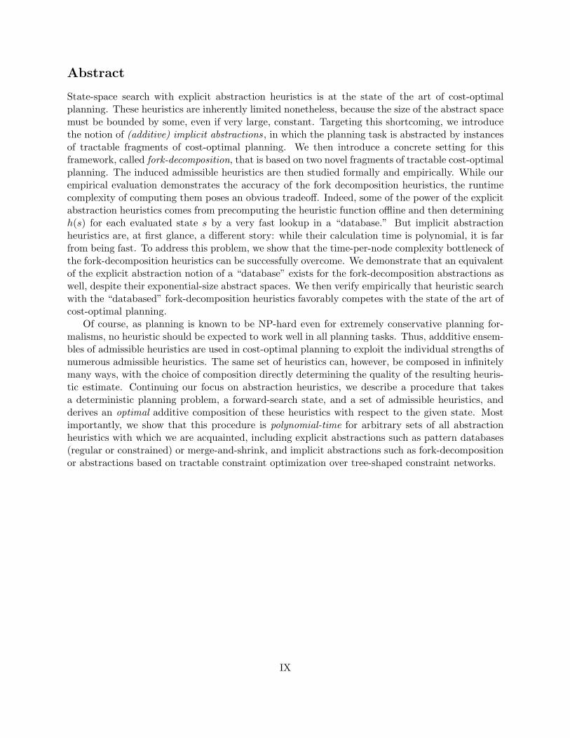
State-space search with explicit abstraction heuristics is at the state of the art of cost-optimalplanning. These heuristics are inherently limited nonetheless, because the size of the abstract spacemust be bounded by some, even if very large, constant. Targeting this shortcoming, we introducethe notion of (additive) implicit abstractions, in which the planning task is abstracted by instancesof tractable fragments of cost-optimal planning. We then introduce a concrete setting for thisframework, called fork-decomposition, that is based on two novel fragments of tractable cost-optimalplanning. The induced admissible heuristics are then studied formally and empirically. While ourempirical evaluation demonstrates the accuracy of the fork decomposition heuristics, the runtimecomplexity of computing them poses an obvious tradeoff. Indeed, some of the power of the explicitabstraction heuristics comes from precomputing the heuristic function offline and then determiningh(s) for each evaluated state s by a very fast lookup in a “database.” But implicit abstractionheuristics are, at first glance, a different story: while their calculation time is polynomial, it is farfrom being fast. To address this problem, we show that the time-per-node complexity bottleneck ofthe fork-decomposition heuristics can be successfully overcome. We demonstrate that an equivalentof the explicit abstraction notion of a “database” exists for the fork-decomposition abstractions aswell, despite their exponential-size abstract spaces. We then verify empirically that heuristic searchwith the “databased” fork-decomposition heuristics favorably competes with the state of the art ofcost-optimal planning.
Of course, as planning is known to be NP-hard even for extremely conservative planning for-malisms, no heuristic should be expected to work well in all planning tasks. Thus, addditive ensem-bles of admissible heuristics are used in cost-optimal planning to exploit the individual strengths ofnumerous admissible heuristics. The same set of heuristics can, however, be composed in infinitelymany ways, with the choice of composition directly determining the quality of the resulting heuris-tic estimate. Continuing our focus on abstraction heuristics, we describe a procedure that takesa deterministic planning problem, a forward-search state, and a set of admissible heuristics, andderives an optimal additive composition of these heuristics with respect to the given state. Mostimportantly, we show that this procedure is polynomial-time for arbitrary sets of all abstractionheuristics with which we are acquainted, including explicit abstractions such as pattern databases(regular or constrained) or merge-and-shrink, and implicit abstractions such as fork-decompositionor abstractions based on tractable constraint optimization over tree-shaped constraint networks.
IX

X
Chapter 1
Introduction
AI problem solving is facing an inherent computational paradox. Most general AI reasoning tasksare known to be very hard, so much so that membership in NP is in itself sometimes perceivedas “good news.” If, however, the intelligence is somehow modeled by a computation, and thecomputation is delegated to the computers, then artificial intelligence has to escape the traps ofintractability as much as possible. Planning is one such reasoning task, corresponding to findinga sequence of state-transforming actions that achieve a goal from the given initial state. It is wellknown that planning is intractable in general (Chapman, 1987), and that even the “simple” classicalplanning with propositional state variables is PSPACE-complete (Bylander, 1994).
While the planning community’s interest in the formal complexity analysis of planning taskshas had its ups and downs, it is now understood that computational tractability is fundamental toall problem solving, for two practical reasons:
1. Planning tasks in automatically controlled real-world systems are believed to be highly struc-tured. If discovered and exploited, this structure may allow for efficient planning (Klein,Jonsson, & Backstrom, 1998). But if this structure is ignored, a general-purpose planner islikely to go on tour in an exponential search space even for tractable tasks. Furthermore,when the overall system is required to provide some guarantees about its run-time complexity,system control cannot be based on worst-case intractable planning theory. The system shouldthus be designed so that planning for it will be provably tractable (Williams & Nayak, 1996,1997).
2. Computational tractability can be an invaluable tool even for problems that fall outside all theknown tractable fragments of planning. For instance, tractable fragments of planning providethe foundations for most (if not all) rigorous heuristic estimates employed in planning asheuristic search (Bonet & Geffner, 2001; Hoffmann, 2003; Helmert, 2006). This is in particulartrue for admissible heuristic functions for planning that are typically defined as the optimalcost of achieving the goals in an over-approximation of the planning task at hand. Such anapproximation is obtained by relaxing or reformulating certain constraints in the specificationof the original task, and the purpose of the approximation is to provide us with a provablytractable planning task (Haslum, 2006; Haslum & Geffner, 2000; Haslum, Bonet, & Geffner,2005; Edelkamp, 2001; Helmert, Haslum, & Hoffmann, 2007).
Unfortunately, the palette of known tractable fragments of planning is still very limited, and thesituation is even more severe for tractable cost-optimal planning. To the best of our knowledge, no
1
more than a few non-trivial fragments of cost-optimal planning are known to be tractable. Whilethere is no difference in the theoretical complexity of satisficing and cost-optimal planning in thegeneral case (Bylander, 1994), many classical planning domains are provably easy to solve but hardto solve optimally (Helmert, 2003). Practice also provides clear evidence for the strikingly differentscalability of satisficing and cost-optimal general-purpose planners (Hoffmann & Edelkamp, 2005).
In this work we exploit computational tractability to boost general cost-optimal planning. Ingeneral, planning algorithms perform reachability analysis in large-scale state models that are im-plicitly described in a concise manner via some intuitive declarative language (Russell & Norvig,2004; Ghallab, Nau, & Traverso, 2004). The use of such a language saves the planning algorithmsfrom being restricted to tasks from a certain domain, e.g., a domain of transportation tasks, butrather allows a wide spectrum of tasks describable in that language. Over the years several suchlanguages were developed and studied; the most popular examples are the classical STRIPS lan-guage (Fikes & Nilsson, 1971), the PDDL language (McDermott, Ghallab, Howe, Kambhampati,Knoblock, Ram, Veloso, Weld, & Wilkins, 1998), and the sas+ language (Backstrom & Klein, 1991;Backstrom & Nebel, 1995). Each such language operates with some notion of initial state, actions,and goal. The initial state describes the state of the world at the starting point, actions allow us tomove from one world state to another, and the goal describes the desirable outcome. Together theyimplicitly define a state model, which explicitly captures the world states and the moves betweenthem (as defined by actions), the initial state, and the set of goal states. In the world of sequentialplanning, the reachability analysis in such a state model corresponds to the search for a path fromthe initial state to some goal state. This path can be viewed as a sequence of corresponding actions,generally named a plan. The cost of such a plan is defined as the sum of the costs of each individualaction along this plan.
Though planning tasks have been studied since the early days of artificial intelligence (Allen,Hendler, & Tate, 1990; Chapman, 1987; Dean & Wellman, 1991; Hendler, Tate, & Drummond,1990; Wilkins, 1984), recent developments have dramatically advanced the field (Geffner, 2002;Ghallab et al., 2004; Weld, 1999). Two main concerns should be addressed in planning, and inparticular, in planning as search. The first is the size of the search space, that is, the number ofsearch states examined before a goal state is found. The size of the search space determines thescalability of the search procedure. The second is the quality of the discovered goal-achieving actionsequence, which should ideally be as cost-efficient as possible. Both concerns can be addressed bycontrolling the order in which the search states are examined. The basic idea is to specify a heuristicfunction h from states to scalars, estimating the cost (of the cheapest path) from states to theirnearest goal state. The search algorithms then take these heuristic estimates as search guides. Inparticular, well-known search algorithms such as A∗ and IDA∗ explore the search nodes s in anon-decreasing order of g(s) +h(s), where g(s) is the true cost of reaching s from the initial searchstate (Hart, Nilsson, & Raphael, 1968; Pearl, 1984; Korf, 1985; Korf & Pearl, 1987; Korf, 1998,1999). If h is admissible, that is, it never overestimates the true cost of reaching the nearest goalstate, then such search algorithms are guaranteed to provide an optimal plan to the goal.
A useful admissible heuristic function must be accurate and efficiently computable. Improvingthe accuracy of a heuristic function without substantially worsening the time complexity of com-puting it usually translates into faster search for optimal solutions. Since the late 1990s, numerousadmissible heuristics for domain-independent planning have been proposed and found practicallyeffective, with research in this direction continuously expanding. Most of the heuristic functionsare based on one of the following four ideas:
2
• The idea of delete-relaxation introduced several heuristics, such as h+ (Hoffmann & Nebel,2001), hmax and hadd (Bonet & Geffner, 2001), hFF (Hoffmann & Nebel, 2001), hpmax (Mirkis& Domshlak, 2007), and hsa (Keyder & Geffner, 2008), with h+ and hmax being the onlyadmissible representatives of this family, while h+ is in general intractable (Bylander, 1994).
• The hm family (Haslum & Geffner, 2000) of critical path heuristics, with the h1 ≡ hmax
member being closely related to the delete relaxation idea, continued the research in thisdirection.
• In parallel, Edelkamp (2001) adapted the ideas of Culberson and Schaeffer (1998) for domain-independent planning, and introduced the first member of the abstraction heuristics family,the pattern database (PDB) heuristic. Several works continued the research in this direction,expanding and generalizing the idea of abstraction heuristics (Edelkamp, 2001; Haslum et al.,2005; Haslum, Botea, Helmert, Bonet, & Koenig, 2007; Helmert et al., 2007).
• Recently, Richter, Helmert, and Westphal (2008) introduced an (inadmissible) landmarksbased heuristic. Shortly after that, several admissible landmark-based heuristics were intro-duced, all closely related to delete relaxation of the planning tasks.
A closer look at these advances in domain-independent admissible heuristics reveals the mainquestion: What constraints should we relax to obtain an effective approximation of the planningtask? In general, an approximation of the planning task can be obtained in several ways. One way isto systematically contract several states to create a single abstract state. Approximations obtainedthis way are called homomorphism abstractions. Most typically, such a state-gluing is obtained byprojecting the original task onto a subset of its parameters, as if ignoring the constraints that falloutside the projection. Homomorphisms have been successfully explored in the scope of domain-independent pattern database (PDB) heuristics (Edelkamp, 2001; Haslum et al., 2005, 2007) andmore general explicit abstraction heuristics (Helmert et al., 2007). Another way of obtaining anover-approximation is to enrich the reachability by adding edges and states in the state-spacetransition graph. Such abstractions are typically referred to as embedding abstractions. The lattertransformation is typically made by abstracting away a certain (either syntacticly or semanticallydefined) class of constraints over the task’s actions. One such embedding abstraction, based oneither full or partial ignoring of negative interactions between the actions, provides the foundationsfor some of the most influential developments in both satisficing and cost-optimal heuristic searchplanning (Bonet & Geffner, 2001; Hoffmann & Nebel, 2001; Refanidis & Vlahavas, 2001; Gerevini,Saetti, & Serina, 2003; Vidal, 2004; Haslum et al., 2005; Haslum, 2006; Bonet & Geffner, 2006;Hoffmann & Brafman, 2006; Domshlak & Hoffmann, 2006; Zhou & Hansen, 2006; Richter et al.,2008; Helmert & Domshlak, 2009).
Generally speaking, an abstraction of a planning task is given by a mapping α : S → Sα
from the states of the planning task’s transition system to the states of some “abstract transitionsystem” such that, for all states s, s′ ∈ S, the cost from α(s) to α(s′) is upper-bounded by thecost from s to s′. The abstraction heuristic value hα(s) is then the cost from α(s) to the closestgoal state of the abstract transition system. Perhaps the most well-known abstraction heuristicsare pattern database (PDB) heuristics, which are based on projecting the planning task onto asubset of its state variables and then explicitly searching for optimal plans in the abstract space.Over the years, PDB heuristics have been shown very effective in several hard search problems,including cost-optimal planning (Culberson & Schaeffer, 1998; Edelkamp, 2001; Felner, Korf, &
3
Hanan, 2004; Haslum et al., 2007). The conceptual limitation of these heuristics, however, is thatthe size of the abstract space and its dimensionality must be fixed.1 The more recent merge-and-shrink abstractions (Helmert et al., 2007) generalize PDB heuristics to overcome the latterlimitation. Instead of perfectly reflecting just a few state variables, merge-and-shrink abstractionsallow all variables to be imperfectly reflected. As demonstrated by the formal and empirical analysisof Helmert et al. (2007), this flexibility often makes the merge-and-shrink abstractions much moreeffective than PDBs. However, the merge-and-shrink abstract spaces are still searched explicitly,and thus they still have to be of fixed size. While quality heuristic estimates can still be obtainedfor many tasks, this limitation is a critical obstacle for many others.
The main objective of our work is to push the envelope of abstraction heuristics beyond explicitabstractions. In keeping with this agenda, we introduce a principled way to obtain abstractionheuristics that limit neither the dimensionality nor the size of the abstract spaces. The basic ideabehind what we call implicit abstractions is simple and intuitive: instead of relying on abstracttasks that are easy to solve because they are small, we can rely on abstract tasks belonging toprovably tractable fragments of cost-optimal planning. The key point is that, at least theoretically,moving to implicit abstractions does away with the requirement that the abstractions be small.Our contribution, however, is far from being of theoretical interest only:
1. We specify acyclic causal-graph decompositions, a general framework for additive implicit ab-stractions that is based on decomposing the task at hand along its causal graph. In this scope,we study the complexity of cost-optimal planning for tasks specified in terms of propositionaland multi-valued state variables, as well as in terms of actions, each of which changes thevalue of a single variable. In some sense, we continue the line of complexity analysis suggestedin (Brafman & Domshlak, 2003), and extend it from satisficing to cost-optimal planning. Ourresults for the first time provide a dividing line between tractable and intractable such prob-lems (Katz & Domshlak, 2008a).
2. We then introduce a concrete family of additive implicit abstractions, called fork decompo-sitions, that are based on two novel fragments of tractable cost-optimal planning (Katz &Domshlak, 2008c). Following the type of analysis suggested by Helmert and Mattmuller(2008), we formally analyze the asymptotic performance ratio of the fork-decompositionheuristics and prove that their worst-case accuracy on selected domains is comparable withthat of (even parametric) state-of-the-art admissible heuristics. We then empirically evalu-ate the accuracy of the fork-decomposition heuristics on a large set of domains from recentplanning competitions and show that their accuracy is competitive with the state of the art.
3. The key attraction of explicit abstractions is that state-to-goal costs in the abstract space canbe precomputed and stored in memory in a preprocessing phase so that heuristic evaluationduring search can be done by a simple lookup. At first view, a necessary condition for pushingcomputation of the heuristic offline appears to be the small size of the abstract space. Weshow, however, that an equivalent of the PDB and merge-and-shrink’s notion of “database”exists for the fork-decomposition abstractions as well, despite the exponential-size abstractspaces of the latter. These databased implicit abstractions are based on a proper partitioningof the heuristic computation into parts that can be shared between search states and partsthat must be computed online per state. Our empirical evaluation shows that A∗ equipped
1This does not necessarily apply to symbolic PDBs which, on some tasks, may exponentially reduce the PDB’srepresentation (Edelkamp, 2002; Ball & Holte, 2008).
4
with the “databased” fork-decomposition heuristics favorably competes with the state of theart of cost-optimal planning (Katz & Domshlak, 2009b).
Of course, as planning is known to be NP-hard even for conservative planning formalisms (By-lander, 1994), no heuristic should be expected to work well in all planning tasks. Moreover, evenfor a fixed planning task, no tractable heuristic will home in on all the “combinatorics” of the taskat hand. The promise, however, is that different heuristics could target different sources of theplanning complexity, and composing a set of heuristics to exploit their individual strengths couldallow a larger range of planning tasks to be solved as well as each individual task to be solved moreefficiently.
Our additional contribution is to the fundamental question of how one should better composea set of admissible heuristics. One of the well-known and heavily-used properties of admissibleheuristics is that taking the maximum of their values maximizes informativeness while preservingadmissibility. A more recent, alternative approach to composing a set of admissible heuristicscorresponds to carefully separating the information used by the different heuristics in the set sothat their values could be summed instead of maximized over. This direction was first exploitedin devising domain-specific heuristics, and more recently in works on additive pattern database(PDB) heuristics (Edelkamp, 2001; Felner et al., 2004; Haslum et al., 2007) and constrained PDBsand m-reachability heuristics (Haslum et al., 2005).
The basic idea underlying all these additive heuristic ensembles is elegantly simple: for eachplanning task’s action a, if it can possibly be counted by more than one heuristic in the ensemble,then one should ensure that the cumulative counting of the cost of a does not exceed its true cost inthe original task. Such action cost partitioning was originally achieved by accounting for the wholecost of each action in computing a single heuristic in the ensemble, while ignoring the cost of thataction in computing all the other heuristics in the ensemble (Edelkamp, 2001; Felner et al., 2004;Haslum et al., 2005). Recently, this “all-in-one/nothing-in-rest” action-cost partitioning has beengeneralized to arbitrary partitioning of the action cost among the heuristics in the ensemble (Katz& Domshlak, 2007a, 2008c; Yang, Culberson, & Holte, 2007; Yang, Culberson, Holte, Zahavi, &Felner, 2008).
The great flexibility of additive heuristic ensembles, however, is a mixed blessing. For better orfor worse, the methodology of taking the maximum over the values provided by an arbitrary set ofindependently constructed admissible heuristics is entirely nonparametric. By contrast, switching toadditive heuristic ensembles requires selecting an action-cost partitioning scheme, and this decisionproblem poses a number of computational challenges:
• The space of alternative action-cost partitions is infinite as the cost of each action can bepartitioned into an arbitrary set of nonnegative real numbers, the sum of which does notexceed the cost of that action.
• At least in domain-independent planning, what we need is a fully unsupervised decisionprocess.
• Last but not least, the relative quality of each action-cost partition (in terms of the accuracyof the resulting additive heuristic) may vary dramatically between the examined search states.Hence, the choice of the action-cost partitioning scheme should ultimately be a function ofthe search state in question.
5
These concerns may explain why all previous works on both domain-specific and domain-independent additive heuristic ensembles adopt this or another ad hoc, fixed choice of action-costpartition. Consequently, all the reported empirical comparative evaluations of various max-basedand additive heuristic ensembles are inconclusive—for some search states along the search pro-cess, the (pre-selected) additive heuristic was found to dominate the max-combination, while forthe other states the opposite was the case. In the context of domain-specific additive PDBs, Yanget al. (2007) conclude that “determining which abstractions [here: action-cost partitioning schemes]will produce additives that are better than max over standards is still a big research issue.”
Focusing on abstraction heuristics, our contribution here is precisely in addressing the problemof choosing the right action-cost partitioning over a given set of heuristics:
1. We provide a procedure that, given (i) a classical planning task Π, (ii) a forward-search states of Π, and (iii) a set of heuristics based on abstractions of Π, derives an optimal action-costpartition for s, that is, a partition that maximizes the heuristic estimate of that state. Theprocedure is fully unsupervised, and is based on a linear programming formulation of thatoptimization problem.
2. We show that the time complexity of our procedure is polynomial for arbitrary sets of allabstraction-based heuristic functions with which we are familiar. Such “procedure-friendly”heuristics include PDBs (Edelkamp, 2001; Yang et al., 2007), constrained PDBs (Haslumet al., 2005), merge-and-shrink abstractions (Helmert et al., 2007), fork-decomposition im-plicit abstractions (Katz & Domshlak, 2008c), and implicit abstractions based on tractableconstraint optimization over tree-shaped constraint networks (Katz & Domshlak, 2008a).Note that the estimate provided by a max-based ensemble corresponds to the estimate pro-vided by the respective additive ensemble under some action-cost partitioning. Thus, byfinding an optimal action-cost partition, we provide a formally complete answer to the afore-mentioned question of “to add or not to add” in the context of abstraction heuristics.
Taking the fork-decomposition abstractions as a case study, we evaluate the empirical effective-ness of switching from ad hoc to optimal additive composition. Our evaluation on a wide rangeof International Planning Competition (IPC) benchmarks shows a substantial reduction in thenumber of nodes expanded by the A∗ algorithm. However, in the standard time-bounded setting,this reduction in expanded nodes is typically negatively balanced by the much more expensiveper-node computation of the optimal additive heuristic. To overcome this pitfall without forfeitingthe promise of optimized action cost partitions altogether, we suggest that optimal action costpartitions be derived only with respect to a subset of evaluated nodes. We examine this approachempirically in its extreme setting where only one optimal action cost partition is computed perplanning task: the one that is optimal for the task’s initial state. This action cost partition is thenused for all the states evaluated by the A∗ algorithm. Our experiments show that even such aconservative use of optimization results in substantial improvement over the same heuristic-searchplanner relying on an ad hoc action cost partition (Katz & Domshlak, 2010).
The rest of the dissertation is organized as follows.
• Chapter 2 presents the essential definitions and constructs used in this work and gives abrief introduction to heuristics and heuristic-search planning, with a focus on the abstractionheuristics.
6
• Chapter 3 presents a study of the computational tractability of cost-optimal planning. Nu-merous new tractable classes of cost-optimal planning are presented (Katz & Domshlak,2007b, 2007a, 2008a). The results are based on exploiting several structural and syntacticcharacteristics of planning tasks such as the structure of their causal graphs.
• Chapter 4 introduces the basic idea and theory behind implicit abstractions (Katz & Domsh-lak, 2007b, 2007a, 2008c, 2009a). The complexity study presented in Chapter 3 plays a majorrole in implementing this theory. We introduce a concrete family of additive implicit ab-stractions, called fork decompositions, which are based on two novel fragments of tractablecost-optimal planning introduced in Chapter 3. Likewise, we develop a “databased” approachto these implicit abstractions and show that they favorably compete with the state of the artof cost-optimal planning.
• Chapter 5 presents the action-cost partitioning framework for composing abstraction-basedheuristics. Such a composition allows us to use multiple abstractions and even multiple typesof abstractions together to obtain more informative estimates. In particular, we show thatthis framework allows for obtaining an optimal cost partitioning in polynomial time, and weshow that all abstraction-based heuristics known to us fit into this framework. In addition,we discuss the possibility of relinquishing the optimality of the composed heuristic for thesake of speed, and show that it favorably competes with the state of the art of cost-optimalplanning.
• Chapter 6 summarizes our work and outlines some current and future work prospects.
For better flow and readability, several detailed constructions were moved to appendices.
• Appendix A describes in detail the complexity results presented in Chapter 3, and
• Appendix B describes the empirical evaluation in detail for several heuristics and cost partitionschemes suggested in Chapters 4-5.
7

8
Chapter 2
Classical Planning, Heuristic Search,and Abstractions
2.1 Planning Tasks and Abstractions
The development of general problem solvers (GPS) has been one of the main goals in operationsresearch, as well as in the artificial intelligence branch of computer science. A general problemsolver is a program that accepts high-level descriptions of problems and automatically computestheir solution. The practical motivation for such solvers is that modeling problems at a high levelis most often simpler than procedurally encoding their solutions. Thus, an effective GPS tool canbe very useful in practice.
A general problem solver must provide the user with a suitable general modeling language fordescribing problems, and general algorithms for solving them. While obtaining a solution using aGPS might be somewhat slower than obtaining it by more specialized methods, this should notnecessarily be the case. Most importantly, the GPS approach typically pays off if developing,implementing, and testing the specialized solution is just too cumbersome, time-consuming, andcost-inefficient (Muscettola, Nayak, Pell, & Williams, 1998). The scope of a general problem solvercan be defined by three elements:
1. mathematical models for making the different planning problems precise,
2. representation languages for describing problems conveniently, and
3. algorithms for solving these problems effectively, often making use of information available intheir representation.
In this work we focus on general solvers for planning problems (Ghallab et al., 2004).Probably the most fundamental class of planning tasks is that of classical planning, correspond-
ing to state models with deterministic actions and complete information. Formally, such a statemodel is a tuple S = 〈S, sI , SG, A, Tr, cost〉 where
- S is a finite set of states, sI ∈ S is the initial state, and SG ⊆ S is a set of alternative goal states,
- A is a finite set of actions, and for each s ∈ S, A(s) ⊆ A denotes the set of all actions applicablein s,
9
Objects Action sas+ representationv ∈ {c1, c2}, {l, l′} ⊆ {A,B,C,D}
Move(v, l, l′) 〈{v = l}, {v = l′}〉v = c3, {l, l′} ⊆ {E,F,G}v = t, {l, l′} ⊆ {D,E}v ∈ {c1, c2, c3}, l ∈ {A,B,C,D,E, F,G}, p ∈ {p1, p2} Load(p, v, l) 〈{p = l, v = l}, {p = v}〉v = t, l ∈ {D,E}, p ∈ {p1, p2} Unload(p, v, l) 〈{p = v, v = l}, {p = l}〉
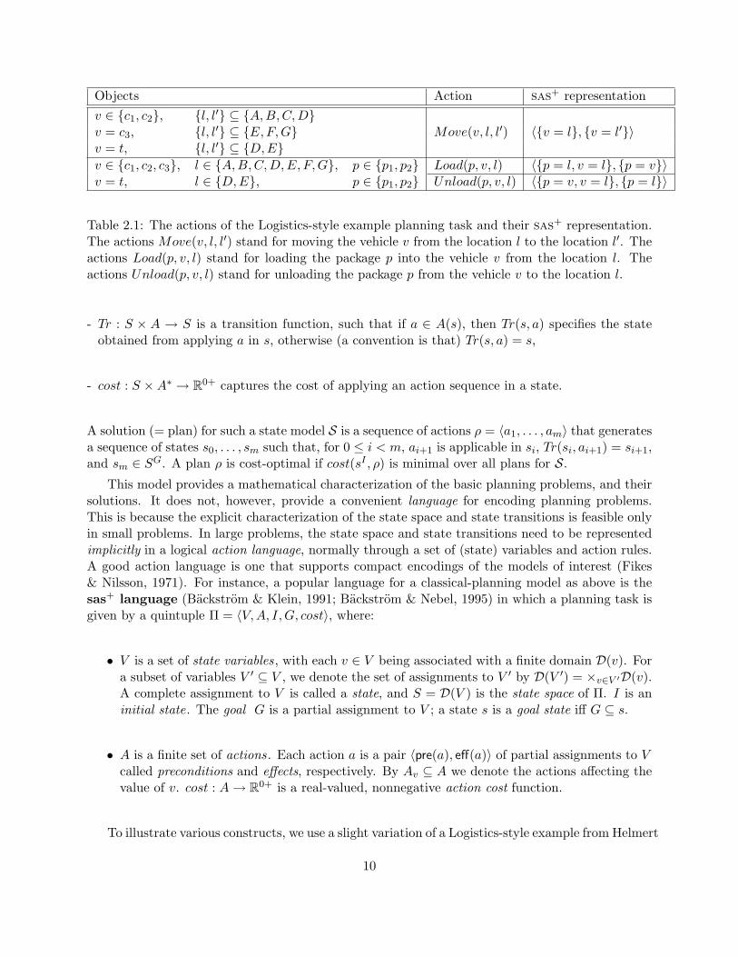
Table 2.1: The actions of the Logistics-style example planning task and their sas+ representation.The actions Move(v, l, l′) stand for moving the vehicle v from the location l to the location l′. Theactions Load(p, v, l) stand for loading the package p into the vehicle v from the location l. Theactions Unload(p, v, l) stand for unloading the package p from the vehicle v to the location l.
- Tr : S × A → S is a transition function, such that if a ∈ A(s), then Tr(s, a) specifies the stateobtained from applying a in s, otherwise (a convention is that) Tr(s, a) = s,
- cost : S ×A∗ → R0+ captures the cost of applying an action sequence in a state.
A solution (= plan) for such a state model S is a sequence of actions ρ = 〈a1, . . . , am〉 that generatesa sequence of states s0, . . . , sm such that, for 0 ≤ i < m, ai+1 is applicable in si, Tr(si, ai+1) = si+1,and sm ∈ SG. A plan ρ is cost-optimal if cost(sI , ρ) is minimal over all plans for S.
This model provides a mathematical characterization of the basic planning problems, and theirsolutions. It does not, however, provide a convenient language for encoding planning problems.This is because the explicit characterization of the state space and state transitions is feasible onlyin small problems. In large problems, the state space and state transitions need to be representedimplicitly in a logical action language, normally through a set of (state) variables and action rules.A good action language is one that supports compact encodings of the models of interest (Fikes& Nilsson, 1971). For instance, a popular language for a classical-planning model as above is thesas+ language (Backstrom & Klein, 1991; Backstrom & Nebel, 1995) in which a planning task isgiven by a quintuple Π = 〈V,A, I,G, cost〉, where:
• V is a set of state variables, with each v ∈ V being associated with a finite domain D(v). Fora subset of variables V ′ ⊆ V , we denote the set of assignments to V ′ by D(V ′) = ×v∈V ′D(v).A complete assignment to V is called a state, and S = D(V ) is the state space of Π. I is aninitial state. The goal G is a partial assignment to V ; a state s is a goal state iff G ⊆ s.
• A is a finite set of actions. Each action a is a pair 〈pre(a), eff(a)〉 of partial assignments to Vcalled preconditions and effects, respectively. By Av ⊆ A we denote the actions affecting thevalue of v. cost : A→ R0+ is a real-valued, nonnegative action cost function.
To illustrate various constructs, we use a slight variation of a Logistics-style example from Helmert
10
A
C
D
B
E
F
G
t
c2
c1c3
p1
p2
c₁ c₂ c₃ t
p₁ p₂
(a) (b)
A
C
D
B
E
F
G
D E at A at B at C at D at E at F at G
in c₂
in c₁ in t
in c₃
(c) (d)
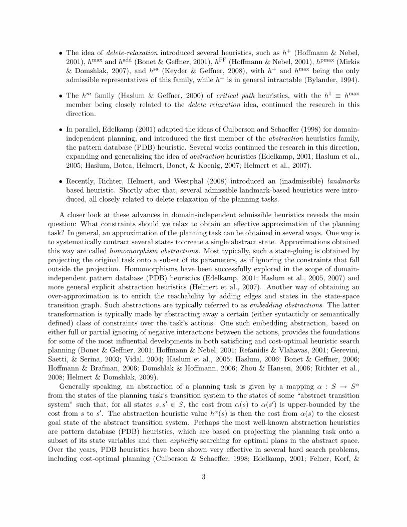
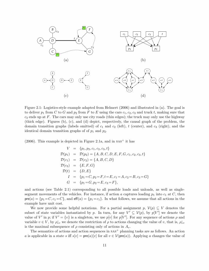
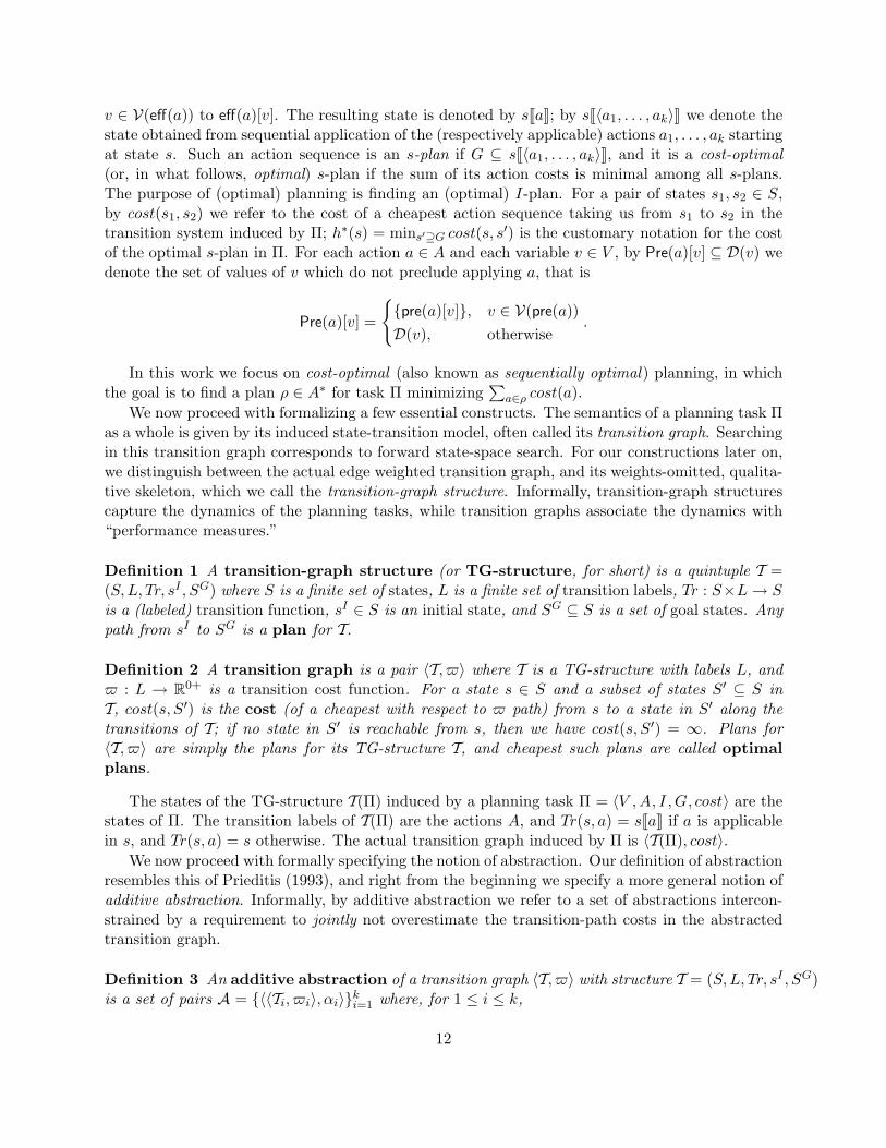
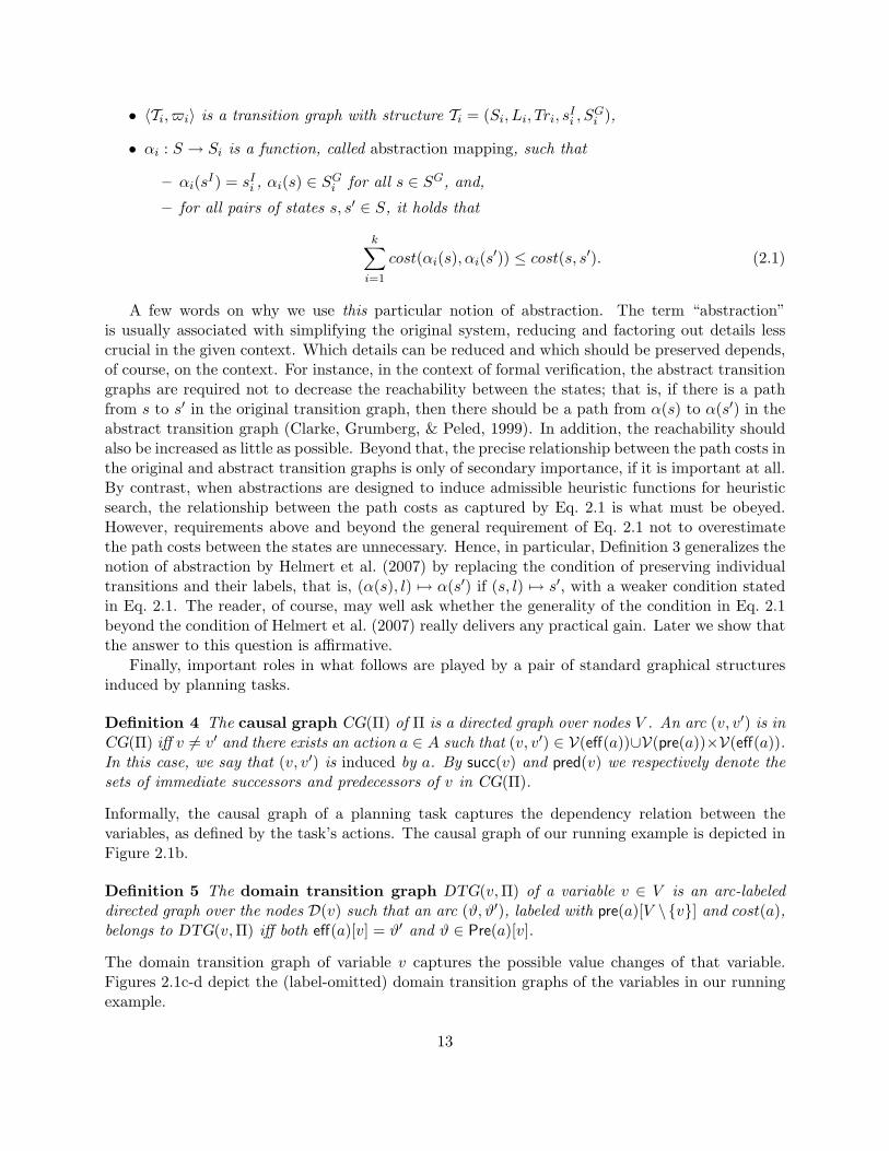
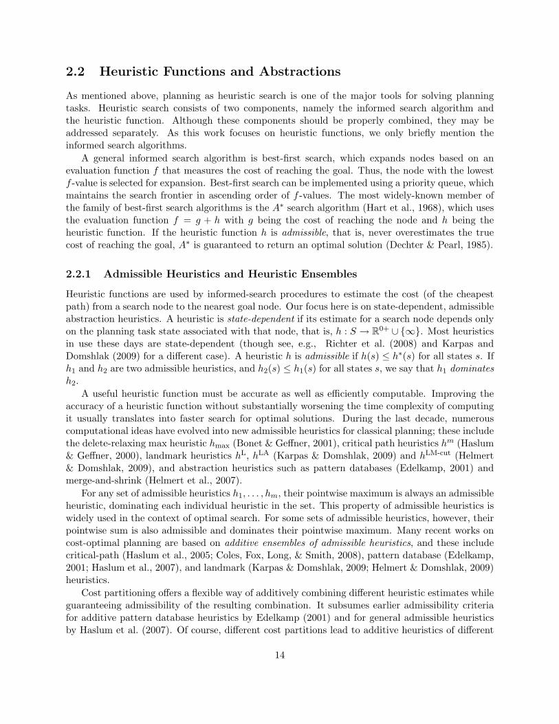
Figure 2.1: Logistics-style example adapted from Helmert (2006) and illustrated in (a). The goal isto deliver p1 from C to G and p2 from F to E using the cars c1, c2, c3 and truck t, making sure thatc3 ends up at F . The cars may only use city roads (thin edges); the truck may only use the highway(thick edge). Figures (b), (c), and (d) depict, respectively, the causal graph of the problem, thedomain transition graphs (labels omitted) of c1 and c2 (left), t (center), and c3 (right), and theidentical domain transition graphs of of p1 and p2.
(2006). This example is depicted in Figure 2.1a, and in sas+ it has
V = {p1, p2, c1, c2, c3, t}D(p1) = D(p2) = {A,B,C,D,E, F,G, c1, c2, c3, t}D(c1) = D(c2) = {A,B,C,D}D(c3) = {E,F,G}D(t) = {D,E}
I = {p1 =C, p2 =F, t=E, c1 =A, c2 =B, c3 =G}G = {p1 =G, p2 =E, c3 =F},
and actions (see Table 2.1) corresponding to all possible loads and unloads, as well as single-segment movements of the vehicles. For instance, if action a captures loading p1 into c1 at C, thenpre(a) = {p1 =C, c1 =C}, and eff(a) = {p1 =c1}. In what follows, we assume that all actions in theexample have unit cost.
We now provide some helpful notations. For a partial assignment p, V(p) ⊆ V denotes thesubset of state variables instantiated by p. In turn, for any V ′ ⊆ V(p), by p[V ′] we denote thevalue of V ′ in p; if V ′ = {v} is a singleton, we use p[v] for p[V ′]. For any sequence of actions ρ andvariable v ∈ V , by ρ↓v we denote the restriction of ρ to actions changing the value of v, that is, ρ↓vis the maximal subsequence of ρ consisting only of actions in Av.
The semantics of actions and action sequences in sas+ planning tasks are as follows. An actiona is applicable in a state s iff s[v] = pre(a)[v] for all v ∈ V(pre(a)). Applying a changes the value of
11
v ∈ V(eff(a)) to eff(a)[v]. The resulting state is denoted by sJaK; by sJ〈a1, . . . , ak〉K we denote thestate obtained from sequential application of the (respectively applicable) actions a1, . . . , ak startingat state s. Such an action sequence is an s-plan if G ⊆ sJ〈a1, . . . , ak〉K, and it is a cost-optimal(or, in what follows, optimal) s-plan if the sum of its action costs is minimal among all s-plans.The purpose of (optimal) planning is finding an (optimal) I-plan. For a pair of states s1, s2 ∈ S,by cost(s1, s2) we refer to the cost of a cheapest action sequence taking us from s1 to s2 in thetransition system induced by Π; h∗(s) = mins′⊇G cost(s, s′) is the customary notation for the costof the optimal s-plan in Π. For each action a ∈ A and each variable v ∈ V , by Pre(a)[v] ⊆ D(v) wedenote the set of values of v which do not preclude applying a, that is
Pre(a)[v] =
{{pre(a)[v]}, v ∈ V(pre(a))D(v), otherwise
.
In this work we focus on cost-optimal (also known as sequentially optimal) planning, in whichthe goal is to find a plan ρ ∈ A∗ for task Π minimizing
∑a∈ρ cost(a).
We now proceed with formalizing a few essential constructs. The semantics of a planning task Πas a whole is given by its induced state-transition model, often called its transition graph. Searchingin this transition graph corresponds to forward state-space search. For our constructions later on,we distinguish between the actual edge weighted transition graph, and its weights-omitted, qualita-tive skeleton, which we call the transition-graph structure. Informally, transition-graph structurescapture the dynamics of the planning tasks, while transition graphs associate the dynamics with“performance measures.”
Definition 1 A transition-graph structure (or TG-structure, for short) is a quintuple T =(S,L, Tr, sI , SG) where S is a finite set of states, L is a finite set of transition labels, Tr : S×L→ Sis a (labeled) transition function, sI ∈ S is an initial state, and SG ⊆ S is a set of goal states. Anypath from sI to SG is a plan for T.
Definition 2 A transition graph is a pair 〈T, $〉 where T is a TG-structure with labels L, and$ : L → R0+ is a transition cost function. For a state s ∈ S and a subset of states S′ ⊆ S inT, cost(s, S′) is the cost (of a cheapest with respect to $ path) from s to a state in S′ along thetransitions of T; if no state in S′ is reachable from s, then we have cost(s, S′) = ∞. Plans for〈T, $〉 are simply the plans for its TG-structure T, and cheapest such plans are called optimalplans.
The states of the TG-structure T(Π) induced by a planning task Π = 〈V ,A, I ,G, cost〉 are thestates of Π. The transition labels of T(Π) are the actions A, and Tr(s, a) = sJaK if a is applicablein s, and Tr(s, a) = s otherwise. The actual transition graph induced by Π is 〈T(Π), cost〉.
We now proceed with formally specifying the notion of abstraction. Our definition of abstractionresembles this of Prieditis (1993), and right from the beginning we specify a more general notion ofadditive abstraction. Informally, by additive abstraction we refer to a set of abstractions intercon-strained by a requirement to jointly not overestimate the transition-path costs in the abstractedtransition graph.
Definition 3 An additive abstraction of a transition graph 〈T, $〉 with structure T = (S,L, Tr, sI , SG)is a set of pairs A = {〈〈Ti, $i〉, αi〉}ki=1 where, for 1 ≤ i ≤ k,
12
• 〈Ti, $i〉 is a transition graph with structure Ti = (Si, Li, Tri, sIi , SGi ),
• αi : S → Si is a function, called abstraction mapping, such that
– αi(sI) = sIi , αi(s) ∈ SGi for all s ∈ SG, and,
– for all pairs of states s, s′ ∈ S, it holds that
k∑i=1
cost(αi(s), αi(s′)) ≤ cost(s, s′). (2.1)
A few words on why we use this particular notion of abstraction. The term “abstraction”is usually associated with simplifying the original system, reducing and factoring out details lesscrucial in the given context. Which details can be reduced and which should be preserved depends,of course, on the context. For instance, in the context of formal verification, the abstract transitiongraphs are required not to decrease the reachability between the states; that is, if there is a pathfrom s to s′ in the original transition graph, then there should be a path from α(s) to α(s′) in theabstract transition graph (Clarke, Grumberg, & Peled, 1999). In addition, the reachability shouldalso be increased as little as possible. Beyond that, the precise relationship between the path costs inthe original and abstract transition graphs is only of secondary importance, if it is important at all.By contrast, when abstractions are designed to induce admissible heuristic functions for heuristicsearch, the relationship between the path costs as captured by Eq. 2.1 is what must be obeyed.However, requirements above and beyond the general requirement of Eq. 2.1 not to overestimatethe path costs between the states are unnecessary. Hence, in particular, Definition 3 generalizes thenotion of abstraction by Helmert et al. (2007) by replacing the condition of preserving individualtransitions and their labels, that is, (α(s), l) 7→ α(s′) if (s, l) 7→ s′, with a weaker condition statedin Eq. 2.1. The reader, of course, may well ask whether the generality of the condition in Eq. 2.1beyond the condition of Helmert et al. (2007) really delivers any practical gain. Later we show thatthe answer to this question is affirmative.
Finally, important roles in what follows are played by a pair of standard graphical structuresinduced by planning tasks.
Definition 4 The causal graph CG(Π) of Π is a directed graph over nodes V . An arc (v, v′) is inCG(Π) iff v 6= v′ and there exists an action a ∈ A such that (v, v′) ∈ V(eff(a))∪V(pre(a))×V(eff(a)).In this case, we say that (v, v′) is induced by a. By succ(v) and pred(v) we respectively denote thesets of immediate successors and predecessors of v in CG(Π).
Informally, the causal graph of a planning task captures the dependency relation between thevariables, as defined by the task’s actions. The causal graph of our running example is depicted inFigure 2.1b.
Definition 5 The domain transition graph DTG(v,Π) of a variable v ∈ V is an arc-labeleddirected graph over the nodes D(v) such that an arc (ϑ, ϑ′), labeled with pre(a)[V \{v}] and cost(a),belongs to DTG(v,Π) iff both eff(a)[v] = ϑ′ and ϑ ∈ Pre(a)[v].
The domain transition graph of variable v captures the possible value changes of that variable.Figures 2.1c-d depict the (label-omitted) domain transition graphs of the variables in our runningexample.
13
2.2 Heuristic Functions and Abstractions
As mentioned above, planning as heuristic search is one of the major tools for solving planningtasks. Heuristic search consists of two components, namely the informed search algorithm andthe heuristic function. Although these components should be properly combined, they may beaddressed separately. As this work focuses on heuristic functions, we only briefly mention theinformed search algorithms.
A general informed search algorithm is best-first search, which expands nodes based on anevaluation function f that measures the cost of reaching the goal. Thus, the node with the lowestf -value is selected for expansion. Best-first search can be implemented using a priority queue, whichmaintains the search frontier in ascending order of f -values. The most widely-known member ofthe family of best-first search algorithms is the A∗ search algorithm (Hart et al., 1968), which usesthe evaluation function f = g + h with g being the cost of reaching the node and h being theheuristic function. If the heuristic function h is admissible, that is, never overestimates the truecost of reaching the goal, A∗ is guaranteed to return an optimal solution (Dechter & Pearl, 1985).
2.2.1 Admissible Heuristics and Heuristic Ensembles
Heuristic functions are used by informed-search procedures to estimate the cost (of the cheapestpath) from a search node to the nearest goal node. Our focus here is on state-dependent, admissibleabstraction heuristics. A heuristic is state-dependent if its estimate for a search node depends onlyon the planning task state associated with that node, that is, h : S → R0+ ∪ {∞}. Most heuristicsin use these days are state-dependent (though see, e.g., Richter et al. (2008) and Karpas andDomshlak (2009) for a different case). A heuristic h is admissible if h(s) ≤ h∗(s) for all states s. Ifh1 and h2 are two admissible heuristics, and h2(s) ≤ h1(s) for all states s, we say that h1 dominatesh2.
A useful heuristic function must be accurate as well as efficiently computable. Improving theaccuracy of a heuristic function without substantially worsening the time complexity of computingit usually translates into faster search for optimal solutions. During the last decade, numerouscomputational ideas have evolved into new admissible heuristics for classical planning; these includethe delete-relaxing max heuristic hmax (Bonet & Geffner, 2001), critical path heuristics hm (Haslum& Geffner, 2000), landmark heuristics hL, hLA (Karpas & Domshlak, 2009) and hLM-cut (Helmert& Domshlak, 2009), and abstraction heuristics such as pattern databases (Edelkamp, 2001) andmerge-and-shrink (Helmert et al., 2007).
For any set of admissible heuristics h1, . . . , hm, their pointwise maximum is always an admissibleheuristic, dominating each individual heuristic in the set. This property of admissible heuristics iswidely used in the context of optimal search. For some sets of admissible heuristics, however, theirpointwise sum is also admissible and dominates their pointwise maximum. Many recent works oncost-optimal planning are based on additive ensembles of admissible heuristics, and these includecritical-path (Haslum et al., 2005; Coles, Fox, Long, & Smith, 2008), pattern database (Edelkamp,2001; Haslum et al., 2007), and landmark (Karpas & Domshlak, 2009; Helmert & Domshlak, 2009)heuristics.
Cost partitioning offers a flexible way of additively combining different heuristic estimates whileguaranteeing admissibility of the resulting combination. It subsumes earlier admissibility criteriafor additive pattern database heuristics by Edelkamp (2001) and for general admissible heuristicsby Haslum et al. (2007). Of course, different cost partitions lead to additive heuristics of different
14
quality, and thus the question of how to automatically derive a good cost partition is of interest.This is precisely the question considered in what follows.
2.2.2 Abstraction Heuristics
Our main focus in this work is on abstraction heuristics. In the most general form an abstractionheuristic is defined as follows.
Definition 6 Let Π be a planning task over states S, and let A = {〈〈Ti, $i〉, αi〉}ki=1 be an additiveabstraction of the transition graph T(Π). If k = O(poly(||Π||)) and, for all states s ∈ S and all1 ≤ i ≤ k, the cost cost(αi(s), SGi ) in 〈Ti, $i〉 is computable in time O(poly(||Π||)), then hA(s) =∑k
i=1 cost(αi(s), SGi ) is an abstraction heuristic function for Π.
Note that admissibility of hA is implied by the cost conservation condition of Eq. 2.1. To furtherillustrate the connection between abstractions and admissible heuristics, consider three well-knownmechanisms for devising admissible planning heuristics: delete relaxation (Bonet & Geffner, 2001),critical-path relaxation (Haslum & Geffner, 2000),1 and pattern database heuristics (Edelkamp,2001).
First, while typically not considered this way, the delete relaxation of a planning task Π =〈V ,A, I ,G, cost〉 does correspond to an abstraction 〈T+ = (S+, L+, Tr+, s
I+, S
G+ , $+), α+〉 of the
transition graph T(Π). Assuming unique naming of the variable values in Π and denoting D+ =⋃v∈V D(v), we have the abstract states S+ being the power-set of D+, and the labels L+ = {a, a+ |
a ∈ A}. The transitions come from two sources: for each abstract state s+ ∈ S+ and each originalaction a ∈ A applicable in s+, we have both Tr+(s+, a) = s+JaK and Tr+(s+, a+) = s+ ∪ eff(a).With a minor abuse of notation, the initial state and the goal states of the abstraction are sI+ = Iand SG+ = {s+ ∈ S+ | s+ ⊇ G}, and the abstraction mapping α+ is simply the identity function. Itis easy to show that, for any state s of our planning task Π, we have cost(α+(s), SG+) = h+(s), whereh+(s) is the delete-relaxation estimate of the cost from s to the goal. As an aside, we note thatthis “delete-relaxation abstraction” 〈T+, α+〉 in particular exemplifies that nothing in Definition 3requires the size of the abstract state space to be limited by the size of the original state space. Inany event, however, the abstraction 〈T+, α+〉 does not induce a heuristic in terms of Definition 6because computing h+(s) is known to be NP-hard (Bylander, 1994).
The situation for critical-path relaxation is exactly the opposite. While computing the corre-sponding family of admissible estimates hm is polynomial-time for any fixed m, this computationis not based on computing the shortest paths in an abstraction of the planning task. The stategraph over which hm is computed is an AND/OR-graph (and not an OR-graph such as transitiongraphs), and the actual computation of hm corresponds to computing a critical tree (and not ashortest path) to the goal. To the best of our knowledge, the precise relation between critical pathand abstraction heuristics is currently an open question (Helmert & Domshlak, 2009).
2.2.3 Explicit Abstractions
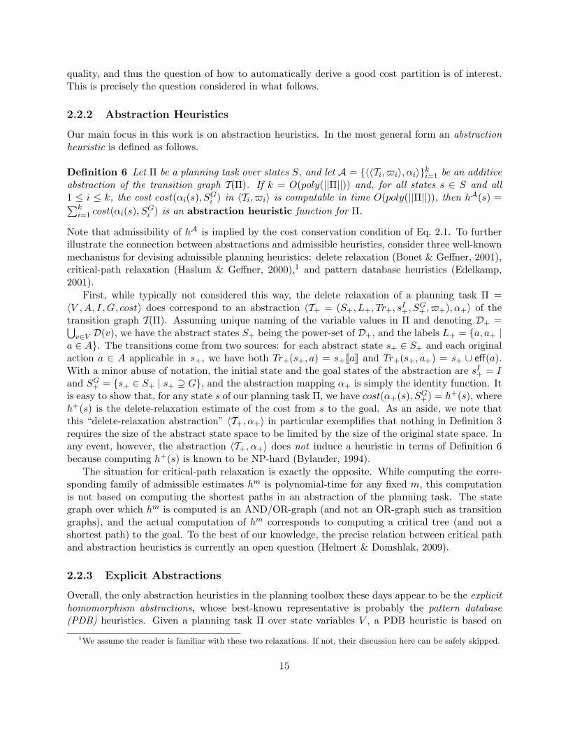
Overall, the only abstraction heuristics in the planning toolbox these days appear to be the explicithomomorphism abstractions, whose best-known representative is probably the pattern database(PDB) heuristics. Given a planning task Π over state variables V , a PDB heuristic is based on
1We assume the reader is familiar with these two relaxations. If not, their discussion here can be safely skipped.
15
projecting Π onto a subset of its variables V α ⊆ V . Such a homomorphism abstraction α maps twostates s1, s2 ∈ S into the same abstract state iff s1[V α] = s2[V α]. Inspired by the (similarly named)domain-specific heuristics for search problems such as (n2−1)-puzzles or Rubik’s Cube (Culberson& Schaeffer, 1998; Hernadvolgyi & Holte, 1999; Felner et al., 2004), PDB heuristics have beensuccessfully exploited in domain-independent planning as well (Edelkamp, 2001, 2002; Haslum et al.,2007). The key decision in constructing PDBs is what sets of variables the problem is projectedto (Edelkamp, 2006; Haslum et al., 2007). However, apart from that need to automatically selectgood projections, the two limitations of PDB heuristics are the size of the abstract space Sα and itsdimensionality. First, the number of abstract states should be small enough to allow reachabilityanalysis in Sα by exhaustive search. Moreover, an O(1) bound on |Sα| is typically set explicitly tofit the time and memory limitations of the system. Second, since PDB abstractions are projections,the explicit constraint on |Sα| implies a fixed-dimensionality constraint |V α| = O(1). In planningtasks with, informally, many alternative resources, this limitation is a pitfall. For instance, suppose{Πi}∞i=1 is a sequence of Logistics problems of growing size with |Vi| = i. If each package in Πi
can be transported by some Θ(i) vehicles, then starting from some i, hα will not account at all formovements of vehicles essential for solving Πi (Helmert & Mattmuller, 2008).
With the goal of preserving the attractiveness of the PDB heuristic while eliminating the bot-tleneck of fixed dimensionality, Helmert et al. (2007) have generalized the methodology of Drager,Finkbeiner, and Podelski (2006) and introduced the so called merge-and-shrink (MS) abstractionsfor planning. MS abstractions are homomorphisms that generalize PDB abstractions by allowingfor more flexibility in selecting the pairs of states to be contracted. The problem’s state spaceis viewed as the synchronized product of its projections onto the single state variables. Startingwith all such “atomic” abstractions, this product can be computed by iteratively composing twoabstract spaces, replacing them with their product. While in a PDB the size of the abstract spaceSα is controlled by limiting the number of product compositions, in MS abstractions it is controlledby interleaving the iterative composition of projections with abstraction of the partial composites.Helmert et al. (2007) have proposed a concrete strategy for this interleaved abstraction/refinementscheme and empirically demonstrated the power of the merge-and-shrink abstraction heuristics.Like PDBs, however, MS abstractions are explicit abstractions, and thus computing their heuristicvalues is also based on explicitly searching for optimal plans in the abstract spaces. Hence, whilemerge-and-shrink abstractions escape the fixed-dimensionality constraint of PDBs, the constrainton the abstract space to be of a fixed size still holds.
16
Chapter 3
Tractable Fragments of Cost-OptimalPlanning
Unfortunately, the palette of known tractable fragments of planning is still very limited, and thesituation is even more severe for tractable optimal planning. To the best of our knowledge, justa few non-trivial fragments of optimal planning are known to be tractable. Despite the identicaltheoretical complexity of regular and optimal planning in the general case (Bylander, 1994), specificplanning domains mostly have different complexity (Helmert, 2003). Clear evidence for strikinglydifferent scalability of satisficing and optimal general-purpose planners can be seen in the resultsof the International Planning Competitions (Hoffmann & Edelkamp, 2005).
In this work we show that the search for new islands of tractability in optimal classical planningis far from exhausted. Specifically, we study the complexity of optimal planning for problemsspecified in terms of propositional state variables and actions, each of which changes the value ofa single variable. In some sense, we continue the line of complexity analysis suggested in Brafmanand Domshlak (2003), and extend it from satisficing to optimal planning. Our results for the firsttime provide a dividing line between tractable and intractable such problems.
Definition 7 A sas+ task Π = 〈V ,A, I ,G, cost〉 belongs to the UB (Unary-effect, Binary-valued)fragment iff all the state variables in V are binary-valued, and each action changes the value ofexactly one variable, that is, for all a ∈ A, we have |eff(a)| = 1.
Different sub-fragments of ub can be defined by placing syntactic and structural restrictions onthe action sets of the problems. For instance, Bylander (1994) shows that planning in ub domainswhere each action is restricted to have only positive preconditions is tractable, yet optimal planningfor this ub fragment is hard. In general, the seminal works of Bylander (1994) and Erol, Nau,and Subrahmanian (1995) indicate that extremely severe syntactic restrictions on single actionsare required to guarantee tractability, or even membership in NP. Backstrom and Klein (1991)consider syntactic restrictions of a more global nature, and show that ub planning is tractable ifthe preconditions of any two actions do not require different values for non-changing variables, andno two actions have the same effect. Interestingly, this fragment of ub, known as PUBS, remainstractable for optimal planning as well. While the characterizing properties of PUBS are veryrestrictive, this result of Backstrom and Klein is an important milestone in planning tractabilityresearch.
Given the limitations of syntactic restrictions observed by Bylander (1994), Erol et al. (1995),
17
v1 v2 v3
v4 v5
v6
v7
v1 v2 v3
v4 v5
v6v7
v1 v2 v3
v4 v5
v6v7
v1 v2 v3
v4 v5
v6
v7
Tree
Inverted Tree
Polytree Directed-path Singly Connected
SP
I
T
!
!
!
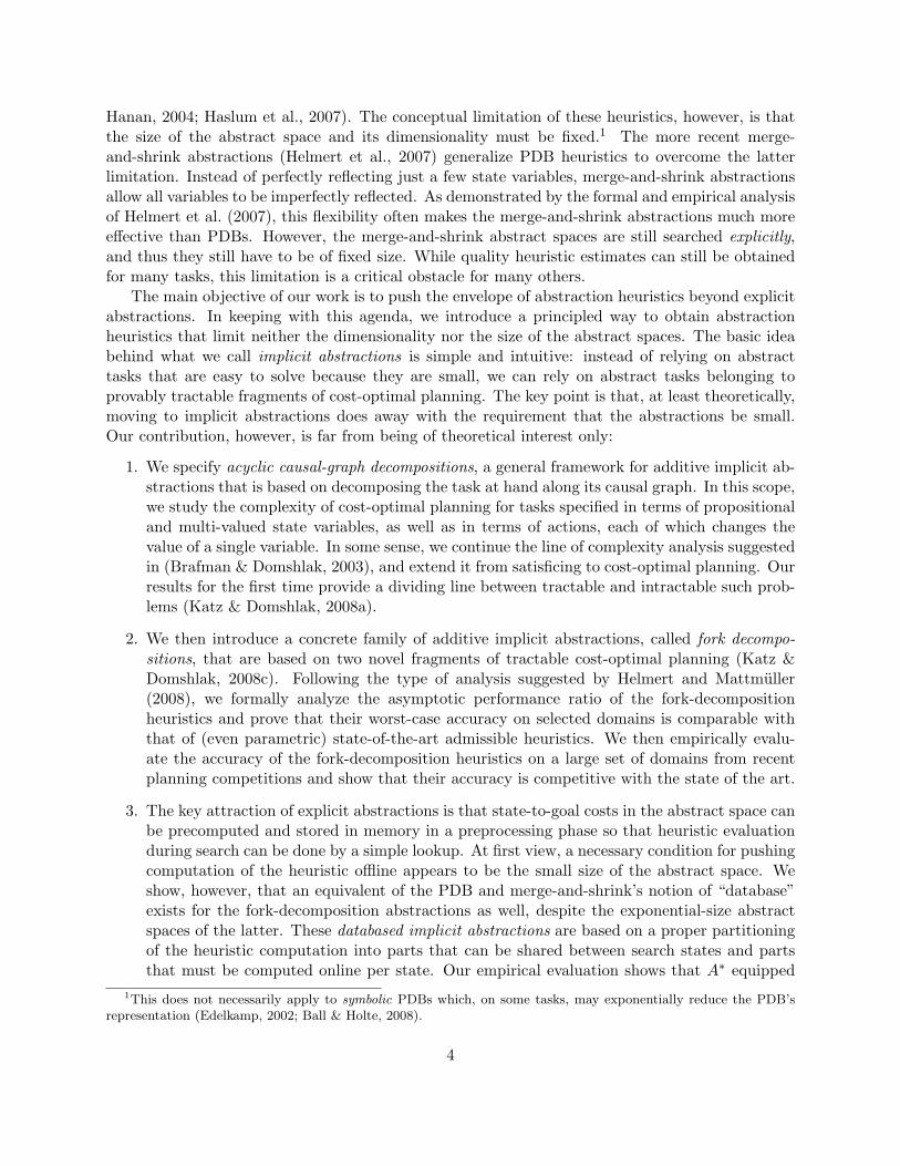
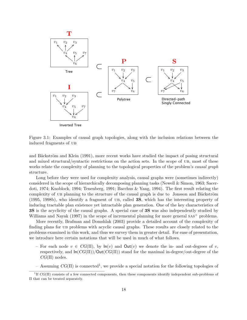
Figure 3.1: Examples of causal graph topologies, along with the inclusion relations between theinduced fragments of ub
and Backstrom and Klein (1991), more recent works have studied the impact of posing structuraland mixed structural/syntactic restrictions on the action sets. In the scope of ub, most of theseworks relate the complexity of planning to the topological properties of the problem’s causal graphstructure.
Long before they were used for complexity analysis, causal graphs were (sometimes indirectly)considered in the scope of hierarchically decomposing planning tasks (Newell & Simon, 1963; Sacer-doti, 1974; Knoblock, 1994; Tenenberg, 1991; Bacchus & Yang, 1994). The first result relating thecomplexity of ub planning to the structure of the causal graph is due to Jonsson and Backstrom(1995, 1998b), who identify a fragment of ub, called 3S, which has the interesting property ofinducing tractable plan existence yet intractable plan generation. One of the key characteristics of3S is the acyclicity of the causal graphs. A special case of 3S was also independently studied byWilliams and Nayak (1997) in the scope of incremental planning for more general sas+ problems.
More recently, Brafman and Domshlak (2003) provide a detailed account of the complexity offinding plans for ub problems with acyclic causal graphs. These results are closely related to theproblems examined in this work, and thus we survey them in greater detail. For ease of presentation,we introduce here certain notations that will be used in much of what follows.
– For each node v ∈ CG(Π), by In(v) and Out(v) we denote the in- and out-degrees of v,respectively, and In(CG(Π))/Out(CG(Π)) stand for the maximal in-degree/out-degree of theCG(Π) nodes.
– Assuming CG(Π) is connected1, we provide a special notation for the following topologies of1If CG(Π) consists of a few connected components, then these components identify independent sub-problems of
Π that can be treated separately.
18
S
Sb Sb
Sbb
P
Pb
Pbb
Pb
T I
S
Sb Sb
Sbb
P
Pb
Pbb
Pb
T I
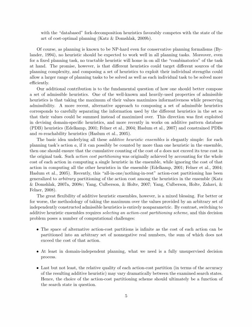
(a) (b)
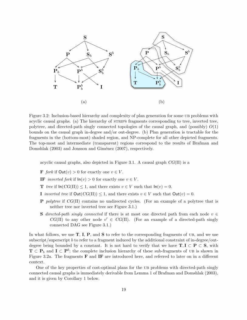
Figure 3.2: Inclusion-based hierarchy and complexity of plan generation for some ub problems withacyclic causal graphs. (a) The hierarchy of strips fragments corresponding to tree, inverted tree,polytree, and directed-path singly connected topologies of the causal graph, and (possibly) O(1)bounds on the causal graph in-degree and/or out-degree. (b) Plan generation is tractable for thefragments in the (bottom-most) shaded region, and NP-complete for all other depicted fragments.The top-most and intermediate (transparent) regions correspond to the results of Brafman andDomshlak (2003) and Jonsson and Gimenez (2007), respectively.
acyclic causal graphs, also depicted in Figure 3.1. A causal graph CG(Π) is a
F fork if Out(v) > 0 for exactly one v ∈ V .
IF inverted fork if In(v) > 0 for exactly one v ∈ V .
T tree if In(CG(Π)) ≤ 1, and there exists v ∈ V such that In(v) = 0.
I inverted tree if Out(CG(Π)) ≤ 1, and there exists v ∈ V such that Out(v) = 0.
P polytree if CG(Π) contains no undirected cycles. (For an example of a polytree that isneither tree nor inverted tree see Figure 3.1.)
S directed-path singly connected if there is at most one directed path from each node v ∈CG(Π) to any other node v′ ∈ CG(Π). (For an example of a directed-path singlyconnected DAG see Figure 3.1.)
In what follows, we use T, I, P, and S to refer to the corresponding fragments of ub, and we usesubscript/superscript b to refer to a fragment induced by the additional constraint of in-degree/out-degree being bounded by a constant. It is not hard to verify that we have T, I ⊂ P ⊂ S, withT ⊂ Pb and I ⊂ Pb; the complete inclusion hierarchy of these sub-fragments of ub is shown inFigure 3.2a. The fragments F and IF are introduced here, and referred to later on in a differentcontext.
One of the key properties of cost-optimal plans for the ub problems with directed-path singlyconnected causal graphs is immediately derivable from Lemma 1 of Brafman and Domshlak (2003),and it is given by Corollary 1 below.
19
Lemma 1 (Brafman and Domshlak (2003)) For any solvable ub task Π with causal graphCG(Π) ∈ S over n state variables, any irreducible plan ρ for Π, and any state variable v in Π, thenumber of value changes of v along ρ is ≤ n, that is, |ρ↓v | ≤ n.
Corollary 1 For any solvable ub task Π with causal graph CG(Π) ∈ S over n state variables, anycost-optimal plan ρ for Π, and any state variable v in Π, we have |ρ↓v | ≤ n.
Given an sas+ planning task Π = 〈V ,A, I ,G, cost〉 and a binary-valued variable v ∈ V , wedenote the initial value I[v] of v by bv, and the opposite value by wv (short for, black/white).Using this notation and exploiting Corollary 1, by σ(v) we denote the longest possible sequenceof values obtainable by v along a cost-optimal plan ρ, with |σ(v)| = n+ 1, bv occupying allthe odd positions of σ(v), and wv occupying all the even positions of σ(v). In addition, by τ(v) wedenote a per-value time-stamping of σ(v)
τ(v) =
{b1v · w1
v · b2v · w2
v · · · bj+1v , n = 2j,
b1v · w1
v · b2v · w2
v · · ·wjv, n = 2j − 1,
, j ∈ N.
The sequences σ(v) and τ(v) play an important role in our constructions both by themselvesand via their prefixes and suffixes. In general, for any sequence S, by �[S] and �[S] we denote theset of all non-empty prefixes and suffixes of S, respectively. In our context, a prefix σ′ ∈ �[σ(v)]is called goal-valid if either the goal value G[v] is unspecified, or the last element of σ′ equals G[v].The set of all goal-valid prefixes of σ(v) is denoted by �∗[σ(v)] ⊆ �[σ(v)]. The notion of goal-validprefixes is also similarly specified for τ(v).
The key tractability result of Brafman and Domshlak (2003) corresponds to a polynomial timeplan generation procedure for Pb, that is, for ub problems inducing polytree causal graphs withall nodes having O(1)-bounded indegree. In addition, Brafman and Domshlak show that plangeneration is NP-complete for the fragment S, and we note that their proof of this claim can beeasily modified to hold for Sbb. These results of tractability and hardness (as well as their immediateimplications) are depicted in Figure 3.2b by the shaded bottom-most and the transparent top-most free-shaped regions. The empty free-shaped region in between corresponds to the gap leftby Brafman and Domshlak (2003). This gap has been recently closed by Jonsson and Gimenez(2007), who prove NP-completeness of plan generation for P. We note that Jonsson and Gimenez’sproof actually carries over to the I fragment as well, and so the gap left by Brafman and Domshlak(2003) is now entirely closed.
3.1 Binary Variable Domains
The complexity results of Brafman and Domshlak (2003) and those of Jonsson and Gimenez (2007)correspond to satisficing planning, and do not distinguish between the plans on the basis of theirquality. By contrast, here we study the complexity of optimal plan generation for ub, focusing on(probably the most canonical) cost-optimal (also known as sequentially-optimal) planning. Cost-optimal planning corresponds to the task of finding a plan ρ ∈ A∗ for Π that minimizes cost(ρ) =∑
a∈ρ cost(a). We provide novel tractability results for cost-optimal planning for ub, and draw adividing line between the tractable and intractable such problems.
In the rest of this section our goal is to adequately describe our results, while most formaldefinitions, constructions, and proofs underlying these results are relegated to appendix A.
20
3.1.1 Cost-optimal planning for Pb
Following Brafman and Domshlak (2003), here we relate the complexity of (cost-optimal) ub plan-ning to the topology of the causal graph. To this end, we consider the structural hierarchy depictedin Figure 3.2a. We begin by considering cost-optimal planning for Pb—it is apparent from Fig-ure 3.2b that this is the most expressive fragment of the hierarchy that is still a candidate fortractable cost-optimal planning. We prove that cost-optimal planning for Pb is tractable and showthat the complexity map of cost-optimal planning for the ub fragments in Figure 3.2a is identicalto that for satisficing planning (that is, Figure 3.2b).
Our algorithm for the Pb fragment is based on compiling a given planning task Π in Pb into aconstraint optimization problem COPΠ = (X ,F) over variables X , functional components F , andthe global objective min
∑ϕ∈F ϕ(X ) such that
(I) COPΠ can be constructed in time polynomial in the description size of Π;
(II) the tree-width of the cost network of COPΠ is bounded by a constant, and the optimaltree-decomposition of the network is given by the compilation process;
(III) if Π is unsolvable then all the assignments to X evaluate the objective function to ∞, andotherwise, the optimum of the global objective is obtained on and only on the assignmentsto X that correspond to cost-optimal plans for Π;
(IV) given an optimal solution to COPΠ, the corresponding cost-optimal plan for Π can be recon-structed from the former in polynomial time.
Having such a compilation scheme, we then solve COPΠ using the standard, poly-time algorithmfor constraint optimization over trees (Dechter, 2003), and find an optimal solution for Π. Thecompilation is based on a certain property of the cost-optimal plans for Pb that allows for conve-niently bounding the number of times each state variable changes its value along such an optimalplan. Given this property of Pb, each state variable v is compiled into a single COP variable xv,and the domain of that COP variable corresponds to all possible sequences of value changes thatv may undergo along a cost-optimal plan. The functional components F are then defined, onefor each COP variable xv, and the scope of such a function captures the “family” of the originalstate variable v in the causal graph, that is, v itself and its immediate predecessors in CG(Π). (SeeAppendix A for the formal definition of the COP, as well as the correctness and complexity claims.)Figure 3.3a depicts a causal graph of a P task Π, with the family of the state variable v4 depictedby the shaded region, and Figure 3.3b shows the cost network induced by compiling Π as a Pb task,with the dashed line surrounding the scope of the functional component induced by the family ofv4. It is not hard to verify that such a cost network induces a tree over variable-families cliques,and for a Pb task, the size of each such clique is bounded by a constant. Hence, the tree-width ofthe cost-network is bounded by a constant as well.
3.1.2 Cost-optimal planning for P(1)
Relaxing the indegree bound brings us to the P fragment of ub, which is NP-hard even for satisficingplanning (Jonsson & Gimenez, 2007). Thus, some additional constraint should be introduced.
21
Causal graphs and k-dependence
While causal graphs provide important information about the structure of planning problems, acloser look at their definition reveals that some accessible information is actually hidden by thisstructure. To start with an example, let us consider the multi-valued encoding of Logistics-styleproblems (Helmert, 2006). In these problems, each variable representing the location of a packagehas as its parents in the causal graph all the variables representing alternative transportationmeans (trucks, planes, etc.), and yet, each individual action affecting the location of a package ispreconditioned by at most one such parent variable. (You cannot load/unload a package into/frommore than one vehicle.) So, even if the in-degree of the causal graph is proportional to some problemdomain parameters, the number of variables that determine applicability of each action may stillbe bounded by a constant.
In other words, while the causal graph provides an aggregate view of the independence rela-tionships between the problem variables, the individual dependencies of the problem actions on thenon-changing variables are suppressed by this view. To exploit these dependencies, we propose a(tangential to the causal graph’s topology) classification of ub problems and study the connectionbetween this classification and the computational tractability of both general and cost-optimal plangeneration for ub.
Definition 8 For any k ∈ Z∗, and any sas+ task Π over actions A, we say that Π is k-dependentif it satisfies |V(pre(a)) \ V(eff(a))| ≤ k for all actions a ∈ A
In other words, an sas+ planning task is k-dependent if no action in its action set depends onmore than k non-changing variables. Putting our two classifications of problems together, for anystructural fragment G of ub (such as, e.g., those in Figure 3.2), and any k ∈ Z∗, by G(k) we denotethe set of all k-dependent problems within G.
Meeting Polytrees and 1-dependence
Recall that the fragment P of ub is NP-hard even for satisficing planning (Jonsson & Gimenez,2007). Our main result here is positive—at least for the most extreme (yet, says the Logisticsexample above, not unrealistic) setting of k = 1, satisfying k-dependence does bring us to an islandof tractability P(1).
Similarly to our treatment of Pb, our algorithm for P(1) exploits the idea of compiling a planningtask Π into a tractable constraint optimization problem COPΠ. However, the planning-to-COPcompilation scheme here is very different from that devised for Pb. In fact, this difference isunavoidable since our construction for Pb relies heavily on the assumption that In(CG(Π)) = O(1),and we do not have this luxury in P(1). Instead, we identify certain properties of the cost-optimalplan sets of the P(1) tasks, and exploit these properties in devising suitable planning-to-COPcompilation schemes.
We begin with considering only P(1) tasks with uniform-cost actions; the cost of a plan forsuch a task is proportional to its length 2. We show that any such solvable task has a cost-optimalplan that makes all the changes of each variable to a certain value using exactly the same (typeof) action. And while devising a correct and tractable planning-to-COP compilation scheme ismore than a step away from identifying this property of P(1), the latter is the cornerstone of whatfollows. This property of P(1) can be used to uniquely compile each state variable v and each
2This is probably the origin of the term “sequential optimality.”
22
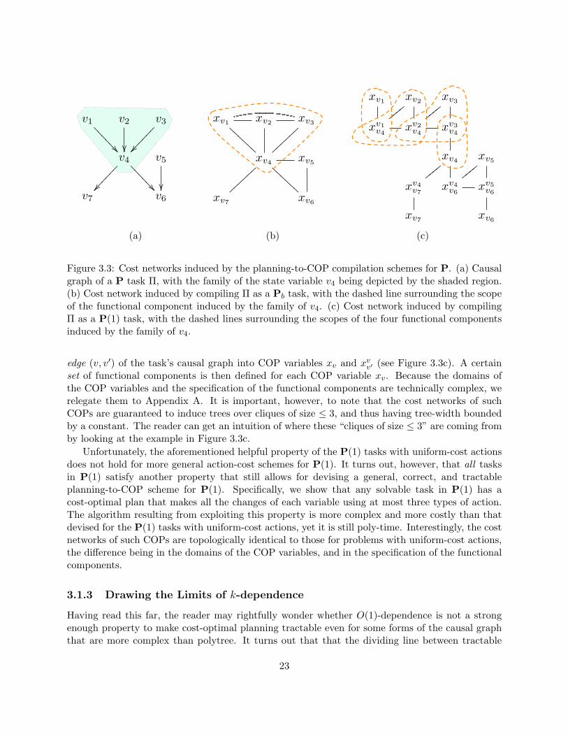
v1
!!!!
!!!!
v2
""
v3
##""""
""
v4
##""""
""
!!!!
!!!!
v5
""v7 v6
xv1xv2
!!!!
xv3
!!!!
xv1
v4x
v2
v4x
v3
v4
xv4
!!!!
xv5
!!!!
xv4
v7x
v4
v6x
v5
v6
xv7xv6
xv1
!!
!!
!!
xv2xv3
""""""
xv4
""""""
!!
!!
!!
xv5
xv7xv6
(a) (b) (c)
Figure 3.3: Cost networks induced by the planning-to-COP compilation schemes for P. (a) Causalgraph of a P task Π, with the family of the state variable v4 being depicted by the shaded region.(b) Cost network induced by compiling Π as a Pb task, with the dashed line surrounding the scopeof the functional component induced by the family of v4. (c) Cost network induced by compilingΠ as a P(1) task, with the dashed lines surrounding the scopes of the four functional componentsinduced by the family of v4.
edge (v, v′) of the task’s causal graph into COP variables xv and xvv′ (see Figure 3.3c). A certainset of functional components is then defined for each COP variable xv. Because the domains ofthe COP variables and the specification of the functional components are technically complex, werelegate them to Appendix A. It is important, however, to note that the cost networks of suchCOPs are guaranteed to induce trees over cliques of size ≤ 3, and thus having tree-width boundedby a constant. The reader can get an intuition of where these “cliques of size ≤ 3” are coming fromby looking at the example in Figure 3.3c.
Unfortunately, the aforementioned helpful property of the P(1) tasks with uniform-cost actionsdoes not hold for more general action-cost schemes for P(1). It turns out, however, that all tasksin P(1) satisfy another property that still allows for devising a general, correct, and tractableplanning-to-COP scheme for P(1). Specifically, we show that any solvable task in P(1) has acost-optimal plan that makes all the changes of each variable using at most three types of action.The algorithm resulting from exploiting this property is more complex and more costly than thatdevised for the P(1) tasks with uniform-cost actions, yet it is still poly-time. Interestingly, the costnetworks of such COPs are topologically identical to those for problems with uniform-cost actions,the difference being in the domains of the COP variables, and in the specification of the functionalcomponents.
3.1.3 Drawing the Limits of k-dependence
Having read this far, the reader may rightfully wonder whether O(1)-dependence is not a strongenough property to make cost-optimal planning tractable even for some forms of the causal graphthat are more complex than polytree. It turns out that that the dividing line between tractable
23
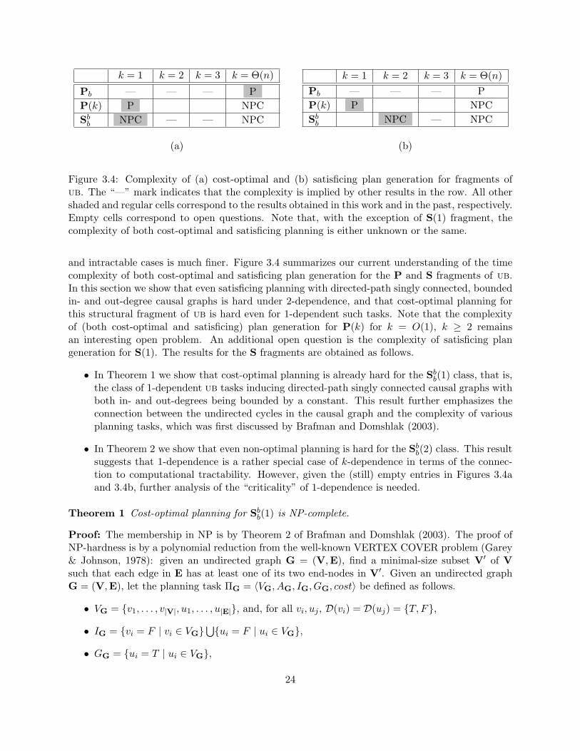
k = 1 k = 2 k = 3 k = Θ(n)
Pb — — — PP(k) P NPCSbb NPC — — NPC
k = 1 k = 2 k = 3 k = Θ(n)Pb — — — PP(k) P NPCSbb NPC — NPC
(a) (b)
Figure 3.4: Complexity of (a) cost-optimal and (b) satisficing plan generation for fragments ofub. The “—” mark indicates that the complexity is implied by other results in the row. All othershaded and regular cells correspond to the results obtained in this work and in the past, respectively.Empty cells correspond to open questions. Note that, with the exception of S(1) fragment, thecomplexity of both cost-optimal and satisficing planning is either unknown or the same.
and intractable cases is much finer. Figure 3.4 summarizes our current understanding of the timecomplexity of both cost-optimal and satisficing plan generation for the P and S fragments of ub.In this section we show that even satisficing planning with directed-path singly connected, boundedin- and out-degree causal graphs is hard under 2-dependence, and that cost-optimal planning forthis structural fragment of ub is hard even for 1-dependent such tasks. Note that the complexityof (both cost-optimal and satisficing) plan generation for P(k) for k = O(1), k ≥ 2 remainsan interesting open problem. An additional open question is the complexity of satisficing plangeneration for S(1). The results for the S fragments are obtained as follows.
• In Theorem 1 we show that cost-optimal planning is already hard for the Sbb(1) class, that is,the class of 1-dependent ub tasks inducing directed-path singly connected causal graphs withboth in- and out-degrees being bounded by a constant. This result further emphasizes theconnection between the undirected cycles in the causal graph and the complexity of variousplanning tasks, which was first discussed by Brafman and Domshlak (2003).
• In Theorem 2 we show that even non-optimal planning is hard for the Sbb(2) class. This resultsuggests that 1-dependence is a rather special case of k-dependence in terms of the connec-tion to computational tractability. However, given the (still) empty entries in Figures 3.4aand 3.4b, further analysis of the “criticality” of 1-dependence is needed.
Theorem 1 Cost-optimal planning for Sbb(1) is NP-complete.
Proof: The membership in NP is by Theorem 2 of Brafman and Domshlak (2003). The proof ofNP-hardness is by a polynomial reduction from the well-known VERTEX COVER problem (Garey& Johnson, 1978): given an undirected graph G = (V,E), find a minimal-size subset V′ of Vsuch that each edge in E has at least one of its two end-nodes in V′. Given an undirected graphG = (V,E), let the planning task ΠG = 〈VG, AG, IG, GG, cost〉 be defined as follows.
• VG = {v1, . . . , v|V|, u1, . . . , u|E|}, and, for all vi, uj , D(vi) = D(uj) = {T, F},
• IG = {vi = F | vi ∈ VG}⋃{ui = F | ui ∈ VG},
• GG = {ui = T | ui ∈ VG},
24
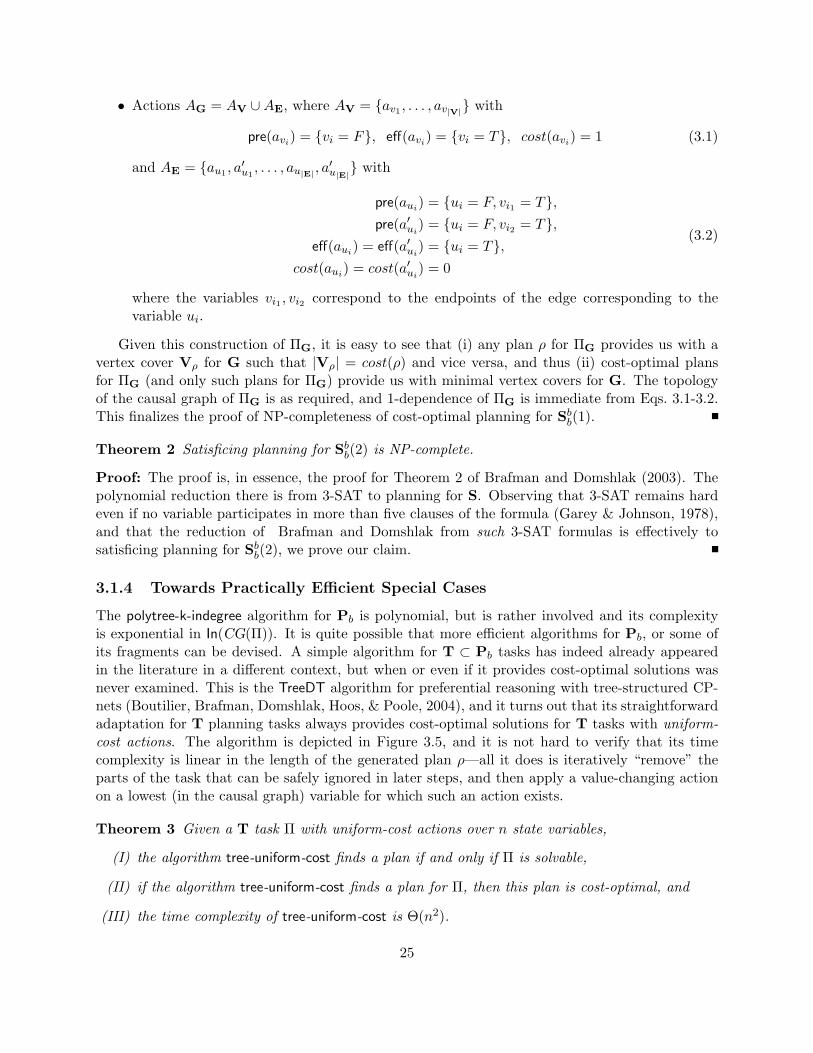
• Actions AG = AV ∪AE, where AV = {av1 , . . . , av|V|} with
pre(avi) = {vi = F}, eff(avi) = {vi = T}, cost(avi) = 1 (3.1)
and AE = {au1 , a′u1, . . . , au|E| , a
′u|E|} with
pre(aui) = {ui = F, vi1 = T},pre(a′ui) = {ui = F, vi2 = T},
eff(aui) = eff(a′ui) = {ui = T},cost(aui) = cost(a′ui) = 0
(3.2)
where the variables vi1 , vi2 correspond to the endpoints of the edge corresponding to thevariable ui.
Given this construction of ΠG, it is easy to see that (i) any plan ρ for ΠG provides us with avertex cover Vρ for G such that |Vρ| = cost(ρ) and vice versa, and thus (ii) cost-optimal plansfor ΠG (and only such plans for ΠG) provide us with minimal vertex covers for G. The topologyof the causal graph of ΠG is as required, and 1-dependence of ΠG is immediate from Eqs. 3.1-3.2.This finalizes the proof of NP-completeness of cost-optimal planning for Sbb(1).
Theorem 2 Satisficing planning for Sbb(2) is NP-complete.
Proof: The proof is, in essence, the proof for Theorem 2 of Brafman and Domshlak (2003). Thepolynomial reduction there is from 3-SAT to planning for S. Observing that 3-SAT remains hardeven if no variable participates in more than five clauses of the formula (Garey & Johnson, 1978),and that the reduction of Brafman and Domshlak from such 3-SAT formulas is effectively tosatisficing planning for Sbb(2), we prove our claim.
3.1.4 Towards Practically Efficient Special Cases
The polytree-k-indegree algorithm for Pb is polynomial, but is rather involved and its complexityis exponential in In(CG(Π)). It is quite possible that more efficient algorithms for Pb, or some ofits fragments can be devised. A simple algorithm for T ⊂ Pb tasks has indeed already appearedin the literature in a different context, but when or even if it provides cost-optimal solutions wasnever examined. This is the TreeDT algorithm for preferential reasoning with tree-structured CP-nets (Boutilier, Brafman, Domshlak, Hoos, & Poole, 2004), and it turns out that its straightforwardadaptation for T planning tasks always provides cost-optimal solutions for T tasks with uniform-cost actions. The algorithm is depicted in Figure 3.5, and it is not hard to verify that its timecomplexity is linear in the length of the generated plan ρ—all it does is iteratively “remove” theparts of the task that can be safely ignored in later steps, and then apply a value-changing actionon a lowest (in the causal graph) variable for which such an action exists.
Theorem 3 Given a T task Π with uniform-cost actions over n state variables,
(I) the algorithm tree-uniform-cost finds a plan if and only if Π is solvable,
(II) if the algorithm tree-uniform-cost finds a plan for Π, then this plan is cost-optimal, and
(III) the time complexity of tree-uniform-cost is Θ(n2).
25
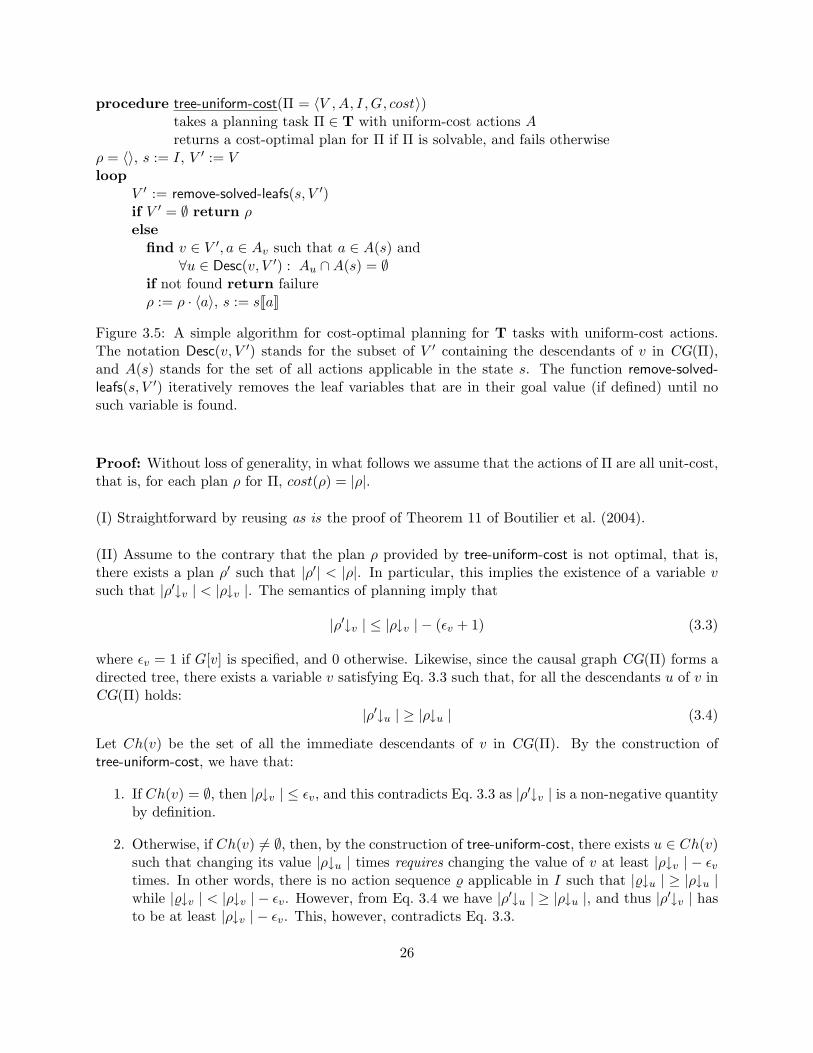
procedure tree-uniform-cost(Π = 〈V ,A, I ,G, cost〉)takes a planning task Π ∈ T with uniform-cost actions Areturns a cost-optimal plan for Π if Π is solvable, and fails otherwise
ρ = 〈〉, s := I, V ′ := Vloop
V ′ := remove-solved-leafs(s, V ′)if V ′ = ∅ return ρelse
find v ∈ V ′, a ∈ Av such that a ∈ A(s) and∀u ∈ Desc(v, V ′) : Au ∩A(s) = ∅
if not found return failureρ := ρ · 〈a〉, s := sJaK
Figure 3.5: A simple algorithm for cost-optimal planning for T tasks with uniform-cost actions.The notation Desc(v, V ′) stands for the subset of V ′ containing the descendants of v in CG(Π),and A(s) stands for the set of all actions applicable in the state s. The function remove-solved-leafs(s, V ′) iteratively removes the leaf variables that are in their goal value (if defined) until nosuch variable is found.
Proof: Without loss of generality, in what follows we assume that the actions of Π are all unit-cost,that is, for each plan ρ for Π, cost(ρ) = |ρ|.
(I) Straightforward by reusing as is the proof of Theorem 11 of Boutilier et al. (2004).
(II) Assume to the contrary that the plan ρ provided by tree-uniform-cost is not optimal, that is,there exists a plan ρ′ such that |ρ′| < |ρ|. In particular, this implies the existence of a variable vsuch that |ρ′↓v | < |ρ↓v |. The semantics of planning imply that
|ρ′↓v | ≤ |ρ↓v | − (εv + 1) (3.3)
where εv = 1 if G[v] is specified, and 0 otherwise. Likewise, since the causal graph CG(Π) forms adirected tree, there exists a variable v satisfying Eq. 3.3 such that, for all the descendants u of v inCG(Π) holds:
|ρ′↓u | ≥ |ρ↓u | (3.4)
Let Ch(v) be the set of all the immediate descendants of v in CG(Π). By the construction oftree-uniform-cost, we have that:
1. If Ch(v) = ∅, then |ρ↓v | ≤ εv, and this contradicts Eq. 3.3 as |ρ′↓v | is a non-negative quantityby definition.
2. Otherwise, if Ch(v) 6= ∅, then, by the construction of tree-uniform-cost, there exists u ∈ Ch(v)such that changing its value |ρ↓u | times requires changing the value of v at least |ρ↓v | − εvtimes. In other words, there is no action sequence % applicable in I such that |%↓u | ≥ |ρ↓u |while |%↓v | < |ρ↓v | − εv. However, from Eq. 3.4 we have |ρ′↓u | ≥ |ρ↓u |, and thus |ρ′↓v | hasto be at least |ρ↓v | − εv. This, however, contradicts Eq. 3.3.
26
Hence, we have proved that |ρ′↓v | ≥ |ρ↓v |, contradicting our assumption that |ρ′| < |ρ|.
(III) Implied by Theorems 12 and 13 of Boutilier et al. (2004).
The requirement in Theorem 3 for all actions to have the same cost is essential. The examplebelow shows that in the more general case the algorithm tree-uniform-cost is no longer cost-optimal.Consider Π = 〈V ,A, I ,G, cost〉 ∈ T with V = {v, u}, I = {bv, bu}, G = {bv,wu}, and A ={a1, a2, a3, a4} with
eff(a1) = {wv}, pre(a1) = {bv}eff(a2) = {bv}, pre(a2) = {wv}eff(a3) = {wu}, pre(a3) = {bu,wv}eff(a4) = {wu}, pre(a4) = {bu, bv}
cost(a1) = cost(a2) = cost(a3) = 1cost(a4) = 4.
On this task, the tree-uniform-cost algorithm returns ρ = 〈a4〉 with cost(ρ) = 4, while the optimalplan is ρ′ = 〈a1, a3, a2〉 with cost(ρ′) = 3.
3.2 General Variable Domains
Investigating the complexity of sas+ fragments beyond ub is not of theoretical interest alone. Re-laxing the unary effectness property leads to complex-structured causal graphs, almost immedietlytaking us beyond the limits of tractability. Unfortunately, relaxing domain bounds altogether alsocan harm the tractability of even the simplest causal graph structures. Domshlak and Dinitz (2001)show that even satisficing planning for sas+ fragments with fork and inverted fork causal graphs isNP-complete. In fact, recent results by Chen and Gimenez (2008) show that planning for any sas+
fragment characterized by any non-trivial connected causal graph is NP-hard. Moreover, even ifthe domain-transition graphs of all the state variables are strongly connected (as in our example),optimal planning for forks and inverted forks remain NP-hard (see Helmert (2003) and (2004) forthe respective results).
While the hardness of optimal planning for problems with fork and inverted fork causal graphscasts a shadow on the relevance of fork-decompositions, a closer look at the proofs of the corre-sponding hardness results of Domshlak and Dinitz (2001) and Helmert (2003, 2004) reveals thatthese proofs rely on root variables having large domains. It turns out that this is not coinciden-tal, and Theorems 4 and 5 below characterize some substantial islands of tractability within thesestructural fragments of sas+.
3.2.1 Cost-optimal planning for F
In order to investigate the complexity of tasks with fork-structured causal graphs and domain-bounded variables, one should distinguish between the bounds on the domains of the leaf variablesand the bound on root domain. Here we present the complexity results for the following two cases:(i) binary root domain and unbounded domains for the leaf variables, and (ii) constant bound onall task variables. Together with the NP-Completeness results for the unbounded root domain case,
27
the only remaining open question is the constant bounded root domain and unbounded domains forthe leaf variables. The tractability proofs for the aforementioned two cases are given in Theorem 4.
Theorem 4 (Tractable Forks) Given a planning task Π = 〈V ,A, I ,G, cost〉 with a fork causalgraph rooted at r, if (i) |D(r)| = 2, or (ii) for all v ∈ V , |D(v)| = O(1), the time complexity of thecost-optimal planning for Π is polynomial in ||Π||.Proof: Observe that, for any planning task Π as in the theorem, the fork structure of the causalgraph CG(Π) implies that all the actions in Π are unary-effect, and each leaf variable v ∈ succ(r)preconditions only the actions affecting v itself. We prove the two cases separately.
First, for |D(r)| = 2, the algorithm below is based on the following three properties satisfied bythe optimal plans ρ for Π.
(i) For any leaf variable v ∈ succ(r), the path ρ↓v from I[v] to G[v] induced by ρ in DTG(v,Π)is either cycle-free or contains only zero-cost cycles. This is the case because otherwise allthe nonzero-cost cycles can be eliminated from ρ↓v while preserving its validity, violating theassumed optimality of ρ. Without loss of generality, in what follows we assume that this pathρ↓v in DTG(v,Π) is cycle-free; in the case of fork causal graphs, we can always select anoptimal ρ that satisfies this requirement for all v ∈ succ(r). Thus, we have |ρ↓v | ≤ |D(v)|−1.
(ii) Having fixed a sequence of value changes of r, the fork’s leaves become mutually independent;that is, our ability to change the value of one does not affect our ability to change the valueof all the others.
(iii) Because r is binary-valued, if v ∈ V \{r} is the “most demanding” leaf variable in terms of thenumber of value changes required from r by the action preconditions along ρ↓v, then these arethe only value changes of r along ρ, except for, possibly, a final value change to G[r]. Thus,in particular, we have |ρ↓r | ≤ maxv∈succ(r) |D(v)|.
We begin with introducing some auxiliary notations. With |D(r)| = 2, without loss of generalitylet D(r) = {0, 1} with I[r] = 0. Let σ(r) be an alternating 0/1 sequence starting with 0, and having0 in all odd and 1 in all even positions. This sequence σ(r) is such that |σ(r)| = 1 if no action in Acan change r’s value to 1, |σ(r)| = 2 if some action can change r’s value to 1 but no action can thenrestore it to value 0, and otherwise, |σ(r)| = 1 + maxv∈succ(r) |D(v)|. Let �∗[σ(r)] be the set of allnonempty prefixes of σ(r) if G[r] is unspecified; otherwise, let it be the set of all nonempty prefixesof σ(r) ending with G[r]. Note that if �∗[σ(r)] = ∅, then the problem is trivially unsolvable; inwhat follows we assume this is not the case. For each v ∈ succ(r), let DTG0
v and DTG1v be the
subgraphs of the domain transition graphs DTG(v,Π), obtained by removing from DTG(v,Π) allthe arcs labeled with r = 1 and r = 0, respectively.
The algorithm below incrementally constructs a set R of valid plans for Π, starting with R = ∅.(1) For each v ∈ succ(r), and each pair of v’s values x, y ∈ D(v), compute the shortest (that is,
cost-minimal) paths π0v(x, y) and π1
v(x, y) from x to y in DTG0v and DTG1
v, respectively. Forsome pairs of values x, y, one or even both these paths may, of course, not exist.
(2) For each sequence σ ∈ �∗[σ(r)], and each v ∈ succ(r), construct a layered digraph Lv(σ) with|σ|+1 node layers L0, . . . , L|σ|, where L0 consists of only I[v], and for 1 ≤ i ≤ |σ|, Li consists of
all nodes y ∈ D(v) for which a path πσ[i]v (x, y) from some node x ∈ Li−1 has been constructed in
step (1). For each x ∈ Li−1, y ∈ Li, Lv(σ) contains an arc (x, y) weighted with cost(πσ[i]v (x, y)).
28
(3) For each σ ∈ �∗[σ(r)], let k = |σ|. A candidate plan ρσ for Π is constructed as follows.
(a) For each v ∈ succ(r), find a cost-minimal path from I[v] to G[v] in Lv(σ). If no such pathexists, then proceed with the next prefix in �∗[σ(r)]. Otherwise, note that the i-th edge onthis path (taking us from some x ∈ Li−1 to some y ∈ Li) corresponds to the cost-minimalpath π
σ[i]v (x, y) from x to y. Let us denote this path from x to y by Siv.
(b) Set R = R∪{ρσ}, where ρσ = S1 · aσ[2] ·S2 · . . . · aσ[k] ·Sk, each sequence Si is obtained byan arbitrary merge of the sequences {Siv}v∈succ(r), and aϑ is the cheapest action changingthe value of r to value ϑ.
(4) If R = ∅, then fail, otherwise return ρ = argminρσ∈R cost(ρσ).
It is straightforward to verify that the complexity of the above procedure is polynomial in thedescription size of Π. To prove correctness, we show that the procedure returns a plan for anysolvable task Π, and that the returned plan ρ′ satisfies cost(ρ′) ≤ cost(ρ) for any optimal plan ρfor Π.
Given a solvable task Π, let ρ be an optimal plan for Π with all ρ↓v for the leaf variablesv being cycle-free. Let ρ↓r= 〈a2 . . . , ak〉; the numbering of actions along ρ↓r starts with a2 tosimplify indexing later on. For each v ∈ succ(r), the actions of ρ↓r divide ρ↓v into subsequencesof v-changing actions ρ↓v= ρ1
v · . . . · ρkv , separated by the value changes required from r. That is,for each 1 ≤ i ≤ k, all actions in ρiv are preconditioned by the same value of r, if any, and if twoactions a ∈ ρiv and a′ ∈ ρi+1
v are preconditioned by r, then pre(a)[r] 6= pre(a′)[r]. Let σ ∈ �∗[σ(r)]be a value sequence such that |σ| = k = |ρ↓r |+ 1. For each v ∈ succ(r), ρ↓v is a path from I[v] toG[v] in Lv(σ), and therefore some ρσ is added into R by the algorithm, meaning that the algorithmfinds a solution. Now, if ρσ ∈ R, then, for each v ∈ succ(r), let S1
v · S2v · . . . · Skv be a cost-minimal
path from I[v] to G[v] in Lv(σ) such that Siv is the sequence of actions changing the value of v andpreconditioned either by r = 0 or nothing for odd i, and by r = 1 or nothing for even i. Thus,
cost(S1v · S2
v · . . . · Skv ) =k∑i=1
cost(Siv) ≤ cost(ρ↓v).
Because sequence Si is obtained by an arbitrary merge of the sequences {Siv}v∈succ(r), and aϑ is thecheapest action changing the value of r to ϑ, then ρσ = S1 · aσ[2] ·S2 · . . . · aσ[k] ·Sk is an applicablesequence of actions that achieves the goal values for each v ∈ succ(r) as well as for r, and
cost(ρσ) = cost(S1 · aσ[2] · S2 · . . . · aσ[k] · Sk) =k∑i=2
cost(aσ[i]) +k∑i=1
cost(Si) ≤
≤cost(ρ↓r) +∑
v∈succ(r)
cost(ρ↓v) = cost(ρ).
Hence, if Π is solvable, then the algorithm returns a plan for Π, and this plan must be optimal.Finally, if Π is not solvable, then R necessarily remains empty, and thus the algorithm fails.
Now we proceed with the second case of the theorem. If |D(v)| = O(1) for all v ∈ V , letd = maxv∈V |D(v)|. Assuming a unified labeling of the values in each D(v) as {1, 2, . . . , |D(v)|},note that (i) there are at most dd different sequences of domain values of size ≤ d, (ii) any plan ρfor Π changes the value of each u ∈ succ(r) according to one such sequence, and (iii) each value
29
change of u along ρ is (possibly) prevailed by some value of r. Hence, the length of a sequenceof r’s values required to support the value changes of succ(r) along a cost-optimal plan for Π isΘ(dd+1). Since each value of r is reachable from another value of r in < d steps, the total numberof value changes of r along a cost-optimal plan for Π is Θ(dd+2).
Given that, we can now generate all possible paths of size ≤ dd+2 from I[r] to G[r] in DTG(r,Π)in time Θ(dd
d+2), and, for each such path, and each u ∈ succ(r), find a minimal-cost path from
I[u] to G[u] in DTG(u,Π) that can be supported by the given path for r. This can be done bygoing over all cycle-free paths in DTG(u,Π) from I[u] to G[u], and checking whether a series ofvalues of r that supports the corresponding actions is a subsequence of the path for r. There areΘ(dd) such paths in DTG(u,Π), and the test per path can be done in time Θ(dd+2). Thus, foreach considered path for r in DTG(r,Π), the respective minimal-cost path for u in DTG(u,Π)can be found in time Θ(d2d+2), and therefore a cost-optimal plan for Π can be found in timeΘ(d2d+2 · ddd+2
) = Θ(ddd+2+2d+2) = O(1).3
3.2.2 Cost-optimal planning for IF
Theorem 5 (Tractable Inverted Forks) Given a planning task Π = 〈V ,A, I ,G, cost〉 with aninverted fork causal graph with sink r ∈ V , if |D(r)| = O(1), the time complexity of the cost-optimalplanning for Π is polynomial in ||Π||.
Proof: Let |D(r)| = d. Observe that the inverted-fork structure of the causal graph CG(Π) impliesthat all the actions in Π are unary-effect, and that the sink r preconditions only the actions affectingr itself. Hence, in what follows we assume that G[r] is specified; otherwise Π breaks down to a setof trivial planning problems over a single variable each. Likewise, from the above properties of Πit follows that, if ρ is an optimal plan for Π, then the path ρ↓r from I[r] to G[r] induced by ρ inDTG(r,Π) is either cycle-free or contains only zero-cost cycles. The latter can be safely eliminatedfrom ρ, and thus we can assume that ρ↓r is cycle-free. Given that, a simple algorithm that finds acost-optimal plan for Π in time Θ(||Π||d + ||Π||3) is as follows.
(1) Create all Θ(|Ar|d−1) cycle-free paths from I[r] to G[r] in DTG(r,Π).
(2) For each variable v ∈ pred(r), and each pair of v’s values x, y ∈ D(v), compute the cost-minimalpath from x to y in DTG(v,Π). The whole set of such cost-minimal paths can be computedusing Θ(d|V |) applications of the Floyd-Warshall algorithm on the domain transition graphsof the sink’s parents pred(r).
(3) For each I[r]-to-G[r] path in DTG(r,Π) generated in step (1), construct a plan for Π based onthat path for r, and the shortest paths computed in (2). This simple construction, depicted inFigure 3.6, is possible because the values of each parent variable can be changed independentlyof the values of all other variables in the inverted fork.
(4) Take the cheapest plan among those constructed in (3). If no plan was constructed in step (3),then Π is unsolvable.
We have already observed that, for each cost-optimal plan ρ, ρ↓r is one of the I[r]-to-G[r]paths generated in step (1). For each v ∈ pred(r), let Sv denote the sequence of values from D(v)
3This constant bound is rather ludicrous, but our construction here is not intended to be complexity-optimaleither. Finding more realistic bounds for this concrete problem is definitely of interest.
30
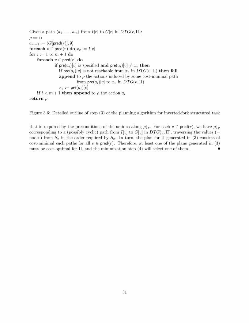
Given a path 〈a1, . . . , am〉 from I[r] to G[r] in DTG(r,Π):ρ := 〈〉am+1 := 〈G[pred(r)], ∅〉foreach v ∈ pred(r) do xv := I[v]for i := 1 to m+ 1 do
foreach v ∈ pred(r) doif pre(ai)[v] is specified and pre(ai)[v] 6= xv then
if pre(ai)[v] is not reachable from xv in DTG(v,Π) then failappend to ρ the actions induced by some cost-minimal path
from pre(ai)[v] to xv in DTG(v,Π)xv := pre(ai)[v]
if i < m+ 1 then append to ρ the action aireturn ρ
Figure 3.6: Detailed outline of step (3) of the planning algorithm for inverted-fork structured task
that is required by the preconditions of the actions along ρ↓r. For each v ∈ pred(r), we have ρ↓vcorresponding to a (possibly cyclic) path from I[v] to G[v] in DTG(v,Π), traversing the values (=nodes) from Sv in the order required by Sv. In turn, the plan for Π generated in (3) consists ofcost-minimal such paths for all v ∈ pred(r). Therefore, at least one of the plans generated in (3)must be cost-optimal for Π, and the minimization step (4) will select one of them.
31

32

Chapter 4
Implicit Abstractions
Over the years, PDB heuristics have been shown to be very effective in several hard search problems,including cost-optimal planning (Culberson & Schaeffer, 1998; Edelkamp, 2001; Felner et al., 2004;Haslum et al., 2007). The conceptual limitation of these heuristics, however, is that the sizeof the abstract space and its dimensionality must be fixed.1 The more recent merge-and-shrinkabstractions generalize PDB heuristics to overcome the latter limitation (Helmert et al., 2007).Instead of perfectly reflecting just a few state variables, merge-and-shrink abstractions allow forimperfectly reflecting all variables. As demonstrated by the formal and empirical analysis of Helmertet al. (2007), this flexibility often makes the merge-and-shrink abstractions much more effective thanPDBs. However, the merge-and-shrink abstract spaces are still searched explicitly, and thus theystill have to be of fixed size. While quality heuristics estimates can still be obtained for manyproblems, this limitation is a critical obstacle for many others.
Our goal in this chapter is to push the envelope of abstraction heuristics beyond explicit ab-stractions. We introduce a principled way to obtain abstraction heuristics that limit neither thedimensionality nor the size of the abstract spaces. The basic idea behind what we call implicitabstractions is simple and intuitive: instead of relying on abstract problems that are easy to solvebecause they are small, we can rely on abstract problems belonging to provably tractable fragmentsof optimal planning. The key point is that, at least theoretically, moving to implicit abstractionsremoves the requirement on the abstractions size to be small. Our contribution, however, is inshowing that implicit abstractions are far from being of theoretical interest only. Specifically,
1. We specify acyclic causal-graph decompositions, a general framework for additive implicit ab-stractions that is based on decomposing the problem at hand along its causal graph. We thenintroduce a concrete family of such abstractions, called fork decompositions, that are based ontwo novel fragments of tractable cost-optimal planning. Following the type of analysis sug-gested by Helmert and Mattmuller (2008), we formally analyze the asymptotic performanceratio of the fork-decomposition heuristics and prove that their worst-case accuracy on selecteddomains is comparable with that of (even parametric) state-of-the-art admissible heuristics.We then empirically evaluate the accuracy of the fork-decomposition heuristics on a large setof domains from recent planning competitions and show that their accuracy is competitivewith the state of the art.
1This does not necessarily apply to symbolic PDBs which, on some tasks, may exponentially reduce the PDB’srepresentation (Edelkamp, 2002).
33
2. The key attraction of explicit abstractions is that costs in the abstract space can be pre-computed and stored in memory in a preprocessing phase so that heuristic evaluation duringsearch can be done by a simple lookup. A necessary condition for this would seem to bethe small size of the abstract space. However, we show that an equivalent of the PDB andmerge-and-shrink’s notion of “database” exists for the fork-decomposition abstractions aswell, despite the exponential-size abstract spaces of the latter. These databased implicit ab-stractions are based on a proper partitioning of the heuristic computation into parts that canbe shared between search states and parts that must be computed online per state. Our em-pirical evaluation shows that A∗ equipped with the “databased” fork-decomposition heuristicsfavorably competes with the state of the art of cost-optimal planning.
This work is a revision and extension of the formulation and results presented by Katz andDomshlak (2008c, 2009b), which in turn is based on ideas first sketched also by Katz and Domshlak(2007a).
4.1 Implicit Abstractions: Basic Idea
Focusing on the O(1) bound posted by explicit abstractions on the size of the abstract space,our first observation is that explicit abstractions are not necessarily the only way to proceed withabstraction heuristics. Given a planning task Π over states S, suppose we can transform it into adifferent planning task Πα such that
1. the transformation induces an abstraction mapping α : S → Sα where Sα is the state spaceof Πα, and
2. both the transformation of Π to Πα, as well as computing α for any state in S, can be donein time polynomial in ||Π||.
Having such planning-task-to-planning-task transformations in mind, we define what we call (ad-ditive) implicit abstractions.
Definition 9 An additive implicit abstraction of a planning task Π is a set of pairs A ={〈Πi, αi〉}ki=1 such that {Πi}ki=1 are some planning tasks and {〈T(Πi), αi〉}ki=1 is an additive ab-straction of T(Π).
Let us now examine the notion of implicit abstractions more closely. First, implicit abstractionsallow for a natural additive combination of admissible heuristics for the abstract tasks. Thiscomposition is formulated below by Theorem 6, extending the original criterion for admissibilityof additive heuristics described in Section 2.1. Second, as formulated by Theorem 7, implicitabstractions can be composed via the functional composition of their abstraction mappings. Thesetwo easy-to-prove properties of implicit abstractions allow us then to take the desired step fromimplicit abstractions to implicit abstraction heuristics.
Theorem 6 (Admissibility) Let Π be a planning task and A = {〈Πi, αi〉}ki=1 be an additiveimplicit abstraction of Π. If, for each 1 ≤ i ≤ k, hi is an admissible heuristic for Πi, then thefunction h(s) =
∑ki=1 hi(αi(s)) is an admissible heuristic for Π.
34
Proof: The proof is straightforward. Let T = (S,L, Tr, sI , SG, $) be the transition graph of Π,and let s be some state in S. For each 1 ≤ i ≤ k, let Ti = (Si, Li, Tri, sIi , S
Gi , $i) be the transition
graph of Πi.First, if hi is an admissible heuristic for Πi, then for all si ∈ SGi ,
hi(αi(s)) ≤ cost(αi(s), si).
Now, for each state s′ ∈ SG, from Definition 3 we have αi(s′) ∈ SGi , and from Eq. 2.1 we have
k∑i=1
cost(αi(s), αi(s′)) ≤ cost(s, s′),
and thus
h(s) =k∑i=1
hi(αi(s)) ≤k∑i=1
cost(αi(s), αi(s′)) ≤ cost(s, s′),
giving us an admissible estimate for h∗(s).
Theorem 7 (Composition) Let Π be a planning task and A = {〈Πi, αi〉}ki=1 be an additive im-plicit abstraction of Π. If, for each 1 ≤ i ≤ k, Ai = {〈Πi,j , αi,j〉}kij=1 is an additive implicitabstraction of Πi, then A′ = ⋃k
i=1{〈Πi,j , αi,j ◦ αi〉}kij=1 is an additive implicit abstraction of Π.
Proof: Let T = (S,L, Tr, sI , SG, $) be the transition graph of Π. For each 1 ≤ i ≤ k, letTi = (Si, Li, Tri, sIi , S
Gi , $i) be the transition graph of Πi, and for each 1 ≤ j ≤ ki, let Ti,j =
(Si,j , Li,j , Tri,j , sIi,j , SGi,j , $i,j) be the transition graph of Πi,j . We need to show that αi,j ◦ αi is an
abstraction mapping as in Definition 3. From αi and αi,j being abstraction mappings, we have
• sIi,j = αi,j(sIi ) = αi,j(αi(sI)) = αi,j ◦ αi(sI),
• for all s ∈ SG we have αi(s) ∈ SGi and thus αi,j(αi(s)) = αi,j ◦ αi(s) ∈ SGi,j , and
• for all si, s′i ∈ Si, cost(si, s′i) ≥∑ki
j=1 cost(αi,j(si), αi,j(s′i)), and thus for all s, s′ ∈ S,
cost(s, s′) ≥k∑i=1
cost(αi(s), αi(s′)) ≥k∑i=1
ki∑j=1
cost(αi,j(αi(s)), αi,j(αi(s′)))
=k∑i=1
ki∑j=1
cost(αi,j ◦ αi(s), αi,j ◦ αi(s′)).
Together, Theorems 6 and 7 suggest the following scheme for deriving abstraction heuristics.Given an additive implicit abstraction A = {〈Πi, αi〉}ki=1, if all its individual abstract tasks belongto some tractable fragments of optimal planning, then we can use in practice the (sum of the)true costs in all Πi as the admissible estimates for the costs in Π. Otherwise, if optimal planningfor some abstract tasks Πi in A cannot be proven polynomial-time solvable, then we can furtherabstract these tasks, obtaining admissible estimates for the true costs in Πi.
35
Definition 10 Let Π be a planning task over states S, and let A = {〈Πi, αi〉}ki=1 be an additiveimplicit abstraction of Π. If k = O(poly(||Π||)), and, for all states s ∈ S and all 1 ≤ i ≤ k,h∗(αi(s)) is polynomial-time computable, then hA(s) =
∑ki=1 h
∗(αi(s)) is an implicit abstractionheuristic function for Π.
Compared to explicit abstraction heuristics such as PDB heuristics and merge-and-shrink heuris-tics, the direction of implicit abstraction heuristics is, at least in principle, appealing because neitherthe dimensionality nor even the size of the state spaces induced by implicit abstractions are requiredto be bounded by something restrictive, if at all. The pitfall, however, is that implicit abstractionheuristics correspond to tractable fragments of optimal planning, and the palette of such knownfragments is extremely limited (Backstrom & Nebel, 1995; Bylander, 1994; Jonsson & Backstrom,1998a; Jonsson, 2007; Katz & Domshlak, 2007b). In fact, none so far has appeared to us veryconvenient for automatically devising useful problem transformations as above. Fortunately, weshow next that the boundaries of tractability can be expanded in the right way, allowing us tosuccessfully materialize the idea of implicit abstraction heuristics.
4.2 Acyclic Causal-Graph Decompositions
In the following, a key role is played by the causal graphs induced by the planning tasks. Informally,the basic idea behind what we call causal-graph decompositions is to abstract the given planningtask Π along a subgraph of Π’s causal graph, with the goal of obtaining abstract problems ofspecific structure. Naturally, there are numerous possibilities for obtaining such structure-orientedabstractions. We now present one such decomposition that is tailored to abstractions around acyclicsubgraphs. Informally, this decomposition can be seen as a sequential application of two kinds oftask transformations: dropping preconditions (Pearl, 1984) and (certain form of) breaking actionswith conjunctive effects into single-effect actions.
Definition 11 Let Π = 〈V ,A, I ,G, cost〉 be a planning task, and let G = (VG , EG) be an acyclicsubgraph of the causal graph CG(Π). A planning task ΠG = 〈VG , AG , IG , GG , costG〉 is an acycliccausal-graph decomposition of Π with respect to G if
1. IG = I[VG ], GG = G[VG ],
2. AG =⋃a∈AAG(a) where each AG(a) = {a1, . . . , al(a)} is a set of actions over VG such that,
for a topological with respect to G ordering of the variables {v1, . . . , vl(a)} = V(eff(a)) ∩ VG,and 1 ≤ i ≤ l(a),
eff(ai)[v] =
{eff(a)[v], v = vi
unspecified, otherwise
pre(ai)[v] =
pre(a)[v], (v, vi) ∈ EG ∧ v 6∈ V(eff(a)) or v = vi
eff(a)[v], (v, vi) ∈ EG ∧ v ∈ V(eff(a))unspecified, otherwise
(4.1)
3. For each action a ∈ A, ∑a′∈AG(a)
costG(a′) ≤ cost(a). (4.2)
36
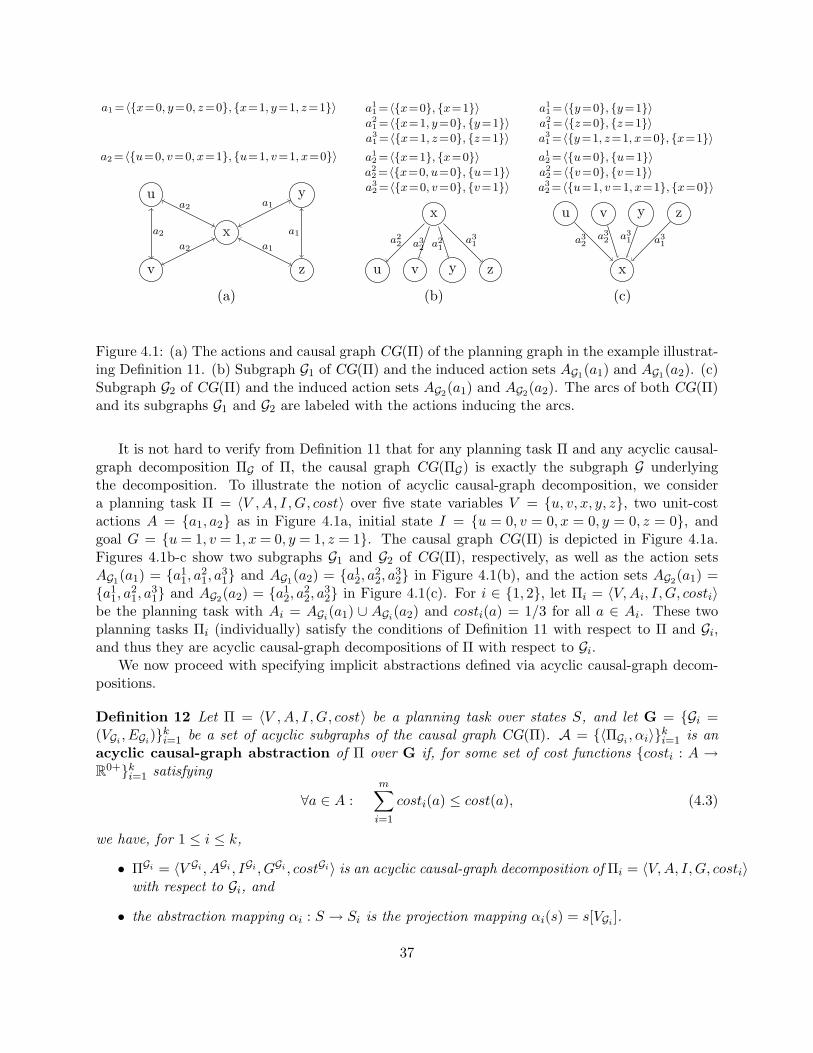
a1 =〈{x=0, y=0, z=0}, {x=1, y=1, z=1}〉
a2 =〈{u=0, v=0, x=1}, {u=1, v=1, x=0}〉
a1
a1
a1
a2
a2
a2
v
u
x
y
z
a11 =〈{x=0}, {x=1}〉a2
1 =〈{x=1, y=0}, {y=1}〉a3
1 =〈{x=1, z=0}, {z=1}〉a1
2 =〈{x=1}, {x=0}〉a2
2 =〈{x=0, u=0}, {u=1}〉a3
2 =〈{x=0, v=0}, {v=1}〉
a22 a3
2 a21
a31
u v
x
y z
a11 =〈{y=0}, {y=1}〉a2
1 =〈{z=0}, {z=1}〉a3
1 =〈{y=1, z=1, x=0}, {x=1}〉a1
2 =〈{u=0}, {u=1}〉a2
2 =〈{v=0}, {v=1}〉a3
2 =〈{u=1, v=1, x=1}, {x=0}〉
a32
a32 a3
1 a31
u v
x
y z
(a) (b) (c)
Figure 4.1: (a) The actions and causal graph CG(Π) of the planning graph in the example illustrat-ing Definition 11. (b) Subgraph G1 of CG(Π) and the induced action sets AG1(a1) and AG1(a2). (c)Subgraph G2 of CG(Π) and the induced action sets AG2(a1) and AG2(a2). The arcs of both CG(Π)and its subgraphs G1 and G2 are labeled with the actions inducing the arcs.
It is not hard to verify from Definition 11 that for any planning task Π and any acyclic causal-graph decomposition ΠG of Π, the causal graph CG(ΠG) is exactly the subgraph G underlyingthe decomposition. To illustrate the notion of acyclic causal-graph decomposition, we considera planning task Π = 〈V ,A, I ,G, cost〉 over five state variables V = {u, v, x, y, z}, two unit-costactions A = {a1, a2} as in Figure 4.1a, initial state I = {u = 0, v = 0, x = 0, y = 0, z = 0}, andgoal G = {u= 1, v = 1, x= 0, y = 1, z = 1}. The causal graph CG(Π) is depicted in Figure 4.1a.Figures 4.1b-c show two subgraphs G1 and G2 of CG(Π), respectively, as well as the action setsAG1(a1) = {a1
1, a21, a
31} and AG1(a2) = {a1
2, a22, a
32} in Figure 4.1(b), and the action sets AG2(a1) =
{a11, a
21, a
31} and AG2(a2) = {a1
2, a22, a
32} in Figure 4.1(c). For i ∈ {1, 2}, let Πi = 〈V,Ai, I, G, costi〉
be the planning task with Ai = AGi(a1) ∪ AGi(a2) and costi(a) = 1/3 for all a ∈ Ai. These twoplanning tasks Πi (individually) satisfy the conditions of Definition 11 with respect to Π and Gi,and thus they are acyclic causal-graph decompositions of Π with respect to Gi.
We now proceed with specifying implicit abstractions defined via acyclic causal-graph decom-positions.
Definition 12 Let Π = 〈V ,A, I ,G, cost〉 be a planning task over states S, and let G = {Gi =(VGi , EGi)}ki=1 be a set of acyclic subgraphs of the causal graph CG(Π). A = {〈ΠGi , αi〉}ki=1 is anacyclic causal-graph abstraction of Π over G if, for some set of cost functions {costi : A →R0+}ki=1 satisfying
∀a ∈ A :m∑i=1
costi(a) ≤ cost(a), (4.3)
we have, for 1 ≤ i ≤ k,
• ΠGi = 〈V Gi , AGi , IGi , GGi , costGi〉 is an acyclic causal-graph decomposition of Πi = 〈V,A, I,G, costi〉with respect to Gi, and
• the abstraction mapping αi : S → Si is the projection mapping αi(s) = s[VGi ].
37
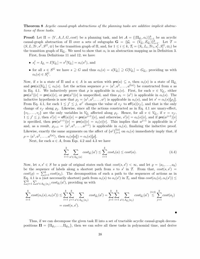
Theorem 8 Acyclic causal-graph abstractions of the planning tasks are additive implicit abstrac-tions of these tasks.
Proof: Let Π = 〈V ,A, I ,G, cost〉 be a planning task, and let A = {〈ΠGi , αi〉}ki=1 be an acycliccausal-graph abstraction of Π over a sets of subgraphs G = {Gi = (VGi , EGi)}ki=1. Let T =(S,L, Tr, sI , SG, $) be the transition graph of Π, and, for 1 ≤ i ≤ k, Ti = (Si, Li, Tri, sIi , S
Gi , $i) be
the transition graph of ΠGi . We need to show that αi is an abstraction mapping as in Definition 3.First, from Definitions 11 and 12, we have
• sIi = IGi = I[VGi ] = sI [VGi ] = αi(sI), and
• for all s ∈ SG we have s ⊇ G and thus αi(s) = s[VGi ] ⊇ G[VGi ] = GGi , providing us withαi(s) ∈ SGi .
Now, if s is a state of Π and a ∈ A is an action with pre(a) ⊆ s, then αi(s) is a state of ΠGiand pre(a)[VGi ] ⊆ αi(s). Let the action sequence ρ = 〈a1, a2, . . . , al(a)〉 be constructed from a asin Eq. 4.1. We inductively prove that ρ is applicable in αi(s). First, for each v ∈ VGi , eitherpre(a1)[v] = pre(a)[v], or pre(a1)[v] is unspecified, and thus ρ1 = 〈a1〉 is applicable in αi(s). Theinductive hypothesis is now that ρj = 〈a1, a2, . . . , aj〉 is applicable in αi(s), and let s′ = αi(s)JρjK.From Eq. 4.1, for each 1 ≤ j′ ≤ j, aj
′changes the value of vj′ to eff(a)[vj′ ], and that is the only
change of vj′ along ρj . Likewise, since all the actions constructed as in Eq. 4.1 are unary-effect,{v1, . . . , vj} are the only variables in VGi affected along ρj . Hence, for all v ∈ VGi , if v = vj′ ,1 ≤ j′ ≤ j, then s′[v] = eff(a)[v] = pre(aj+1)[v], and otherwise, s′[v] = αi(s)[v], and if pre(aj+1)[v]is specified, then pre(aj+1)[v] = pre(a)[v] = αi(s)[v]. This implies that aj+1 is applicable in s′
and, as a result, ρj+1 = 〈a1, a2, . . . , aj+1〉 is applicable in αi(s), finalizing the inductive proof.Likewise, exactly the same arguments on the affect of {aj}l(a)
j=1 on αi(s) immediately imply that, ifρ = 〈a1, a2, . . . , al(a)〉, then αi(sJaK) = αi(s)JρK.
Next, for each a ∈ A, from Eqs. 4.2 and 4.3 we have
k∑i=1
∑a′∈AGi (a)
costGi(a′) ≤
k∑i=1
costi(a) ≤ cost(a). (4.4)
Now, let s, s′ ∈ S be a pair of original states such that cost(s, s′) < ∞, and let % = 〈a1, . . . , ak〉be the sequence of labels along a shortest path from s to s′ in T. From that, cost(s, s′) =cost(%) =
∑kj=1 cost(aj). The decomposition of such a path to the sequences of actions as in
Eq. 4.1 is a (not neccesarily shortest) path from αi(s) to αi(s′) in Ti, and thus cost(αi(s), αi(s′)) ≤∑kj=1
∑a′∈AGi (aj)
costGi(a′), providing us with
k∑i=1
cost(αi(s), αi(s′)) ≤k∑i=1
k∑j=1
∑a′∈AGi (aj)
costGi(a′) =
k∑j=1
k∑i=1
∑a′∈AGi (aj)
costGi(a′)
(4.4)
≤k∑j=1
cost(aj)
= cost(s, s′).
Thus, if we can decompose the given task Π into a set of tractable acyclic causal-graph decom-positions Π = {ΠG1 , . . . ,ΠGm}, then we can solve all these tasks in polynomial time, and derive
38
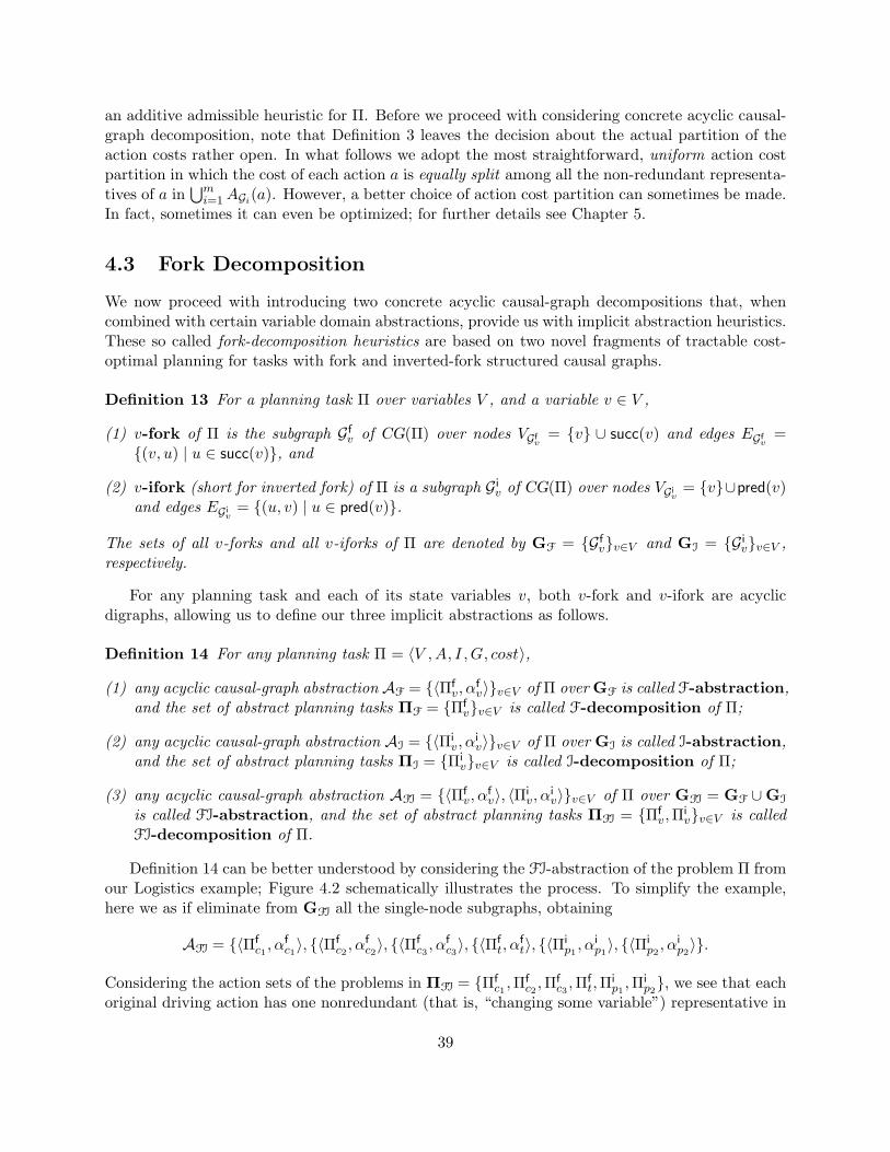
an additive admissible heuristic for Π. Before we proceed with considering concrete acyclic causal-graph decomposition, note that Definition 3 leaves the decision about the actual partition of theaction costs rather open. In what follows we adopt the most straightforward, uniform action costpartition in which the cost of each action a is equally split among all the non-redundant representa-tives of a in
⋃mi=1AGi(a). However, a better choice of action cost partition can sometimes be made.
In fact, sometimes it can even be optimized; for further details see Chapter 5.
4.3 Fork Decomposition
We now proceed with introducing two concrete acyclic causal-graph decompositions that, whencombined with certain variable domain abstractions, provide us with implicit abstraction heuristics.These so called fork-decomposition heuristics are based on two novel fragments of tractable cost-optimal planning for tasks with fork and inverted-fork structured causal graphs.
Definition 13 For a planning task Π over variables V , and a variable v ∈ V ,
(1) v-fork of Π is the subgraph Gfv of CG(Π) over nodes VGf
v= {v} ∪ succ(v) and edges EGf
v=
{(v, u) | u ∈ succ(v)}, and
(2) v-ifork (short for inverted fork) of Π is a subgraph G iv of CG(Π) over nodes VG i
v= {v}∪pred(v)
and edges EG iv
= {(u, v) | u ∈ pred(v)}.
The sets of all v-forks and all v-iforks of Π are denoted by GF = {Gfv}v∈V and GI = {G i
v}v∈V ,respectively.
For any planning task and each of its state variables v, both v-fork and v-ifork are acyclicdigraphs, allowing us to define our three implicit abstractions as follows.
Definition 14 For any planning task Π = 〈V ,A, I ,G, cost〉,
(1) any acyclic causal-graph abstraction AF = {〈Πfv, α
fv〉}v∈V of Π over GF is called F-abstraction,
and the set of abstract planning tasks ΠF = {Πfv}v∈V is called F-decomposition of Π;
(2) any acyclic causal-graph abstraction AI = {〈Πiv, α
iv〉}v∈V of Π over GI is called I-abstraction,
and the set of abstract planning tasks ΠI = {Πiv}v∈V is called I-decomposition of Π;
(3) any acyclic causal-graph abstraction AFI = {〈Πfv, α
fv〉, 〈Πi
v, αiv〉}v∈V of Π over GFI = GF ∪GI
is called FI-abstraction, and the set of abstract planning tasks ΠFI = {Πfv,Π
iv}v∈V is called
FI-decomposition of Π.
Definition 14 can be better understood by considering the FI-abstraction of the problem Π fromour Logistics example; Figure 4.2 schematically illustrates the process. To simplify the example,here we as if eliminate from GFI all the single-node subgraphs, obtaining
AFI = {〈Πfc1 , α
fc1〉, {〈Πf
c2 , αfc2〉, {〈Πf
c3 , αfc3〉, {〈Πf
t, αft〉, {〈Πi
p1, αi
p1〉, {〈Πi
p2, αi
p2〉}.
Considering the action sets of the problems in ΠFI = {Πfc1 ,Π
fc2 ,Π
fc3 ,Π
ft,Π
ip1,Πi
p2}, we see that each
original driving action has one nonredundant (that is, “changing some variable”) representative in
39
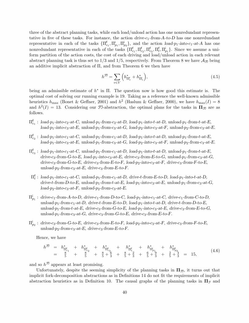
three of the abstract planning tasks, while each load/unload action has one nonredundant represen-tative in five of these tasks. For instance, the action drive-c1-from-A-to-D has one nonredundantrepresentative in each of the tasks {Πf
c1 ,Πip1,Πi
p2}, and the action load-p1-into-c1-at-A has one
nonredundant representative in each of the tasks {Πfc1 ,Π
fc2 ,Π
fc3 ,Π
ft,Π
ip1}. Since we assume a uni-
form partition of the action costs, the cost of each driving and load/unload action in each relevantabstract planning task is thus set to 1/3 and 1/5, respectively. From Theorem 8 we have AFI beingan additive implicit abstraction of Π, and from Theorem 6 we then have
hFI =∑v∈V
(h∗Πf
v+ h∗Πi
v
), (4.5)
being an admissible estimate of h∗ in Π. The question now is how good this estimate is. Theoptimal cost of solving our running example is 19. Taking as a reference the well-known admissibleheuristics hmax (Bonet & Geffner, 2001) and h2 (Haslum & Geffner, 2000), we have hmax(I) = 8and h2(I) = 13. Considering our FI-abstraction, the optimal plans for the tasks in ΠFI are asfollows.
Πfc1 : load-p1-into-c2-at-C, unload-p1-from-c2-at-D, load-p1-into-t-at-D, unload-p1-from-t-at-E,
load-p1-into-c3-at-E, unload-p1-from-c3-at-G, load-p2-into-c3-at-F, unload-p2-from-c3-at-E.
Πfc2 : load-p1-into-c1-at-C, unload-p1-from-c1-at-D, load-p1-into-t-at-D, unload-p1-from-t-at-E,
load-p1-into-c3-at-E, unload-p1-from-c3-at-G, load-p2-into-c3-at-F, unload-p2-from-c3-at-E.
Πfc3 : load-p1-into-c1-at-C, unload-p1-from-c1-at-D, load-p1-into-t-at-D, unload-p1-from-t-at-E,
drive-c3-from-G-to-E, load-p1-into-c3-at-E, drive-c3-from-E-to-G, unload-p1-from-c3-at-G,drive-c3-from-G-to-E, drive-c3-from-E-to-F, load-p2-into-c3-at-F, drive-c3-from-F-to-E,unload-p2-from-c3-at-E, drive-c3-from-E-to-F.
Πft : load-p1-into-c1-at-C, unload-p1-from-c1-at-D, drive-t-from-E-to-D, load-p1-into-t-at-D,
drive-t-from-D-to-E, unload-p1-from-t-at-E, load-p1-into-c3-at-E, unload-p1-from-c3-at-G,load-p2-into-c3-at-F, unload-p2-from-c3-at-E.
Πip1
: drive-c1-from-A-to-D, drive-c1-from-D-to-C, load-p1-into-c1-at-C, drive-c1-from-C-to-D,unload-p1-from-c1-at-D, drive-t-from-E-to-D, load-p1-into-t-at-D, drive-t-from-D-to-E,unload-p1-from-t-at-E, drive-c3-from-G-to-E, load-p1-into-c3-at-E, drive-c3-from-E-to-G,unload-p1-from-c3-at-G, drive-c3-from-G-to-E, drive-c3-from-E-to-F.
Πip2
: drive-c3-from-G-to-E, drive-c3-from-E-to-F, load-p2-into-c3-at-F, drive-c3-from-F-to-E,unload-p2-from-c3-at-E, drive-c3-from-E-to-F.
Hence, we have
hFI = h∗Πfc1
+ h∗Πfc2
+ h∗Πfc3
+ h∗Πft
+ h∗Πip1
+ h∗Πfp2
= 85 + 8
5 + 85 + 6
3 + 85 + 2
3 + 65 + 9
3 + 25 + 4
3 = 15,(4.6)
and so hFI appears at least promising.Unfortunately, despite the seeming simplicity of the planning tasks in ΠFI, it turns out that
implicit fork-decomposition abstractions as in Definitions 14 do not fit the requirements of implicitabstraction heuristics as in Definition 10. The causal graphs of the planning tasks in ΠF and
40
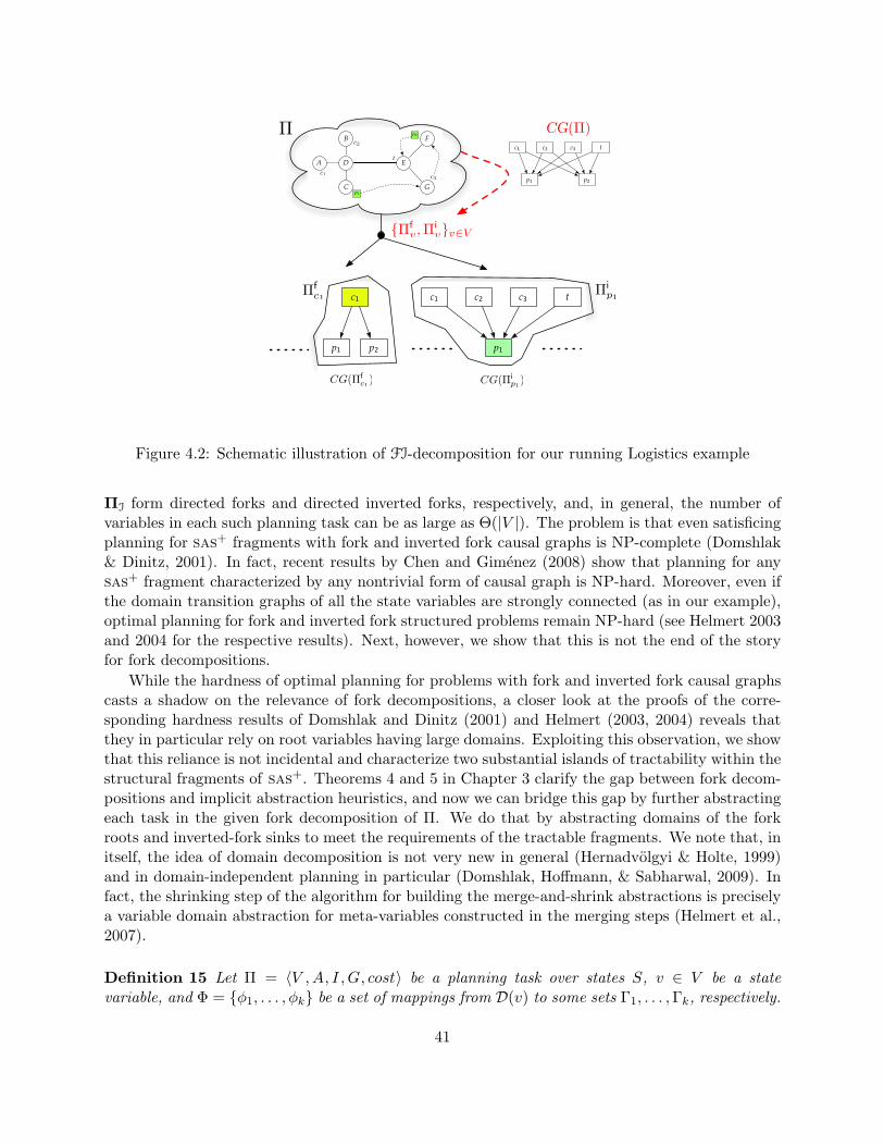
c! c" c# t
p! p"
c!
p! p"
c! c" c# t
p!
CG(!fc1
) CG(!ifp1
)
A
C
D
B
E
F
G
t
c2
c1 c3
p1
p2CG(!)!
CG(!ip1
)CG(!fc1
)
!fc1
!ip1
{!fv,!i
v}v!V
Figure 4.2: Schematic illustration of FI-decomposition for our running Logistics example
ΠI form directed forks and directed inverted forks, respectively, and, in general, the number ofvariables in each such planning task can be as large as Θ(|V |). The problem is that even satisficingplanning for sas+ fragments with fork and inverted fork causal graphs is NP-complete (Domshlak& Dinitz, 2001). In fact, recent results by Chen and Gimenez (2008) show that planning for anysas+ fragment characterized by any nontrivial form of causal graph is NP-hard. Moreover, even ifthe domain transition graphs of all the state variables are strongly connected (as in our example),optimal planning for fork and inverted fork structured problems remain NP-hard (see Helmert 2003and 2004 for the respective results). Next, however, we show that this is not the end of the storyfor fork decompositions.
While the hardness of optimal planning for problems with fork and inverted fork causal graphscasts a shadow on the relevance of fork decompositions, a closer look at the proofs of the corre-sponding hardness results of Domshlak and Dinitz (2001) and Helmert (2003, 2004) reveals thatthey in particular rely on root variables having large domains. Exploiting this observation, we showthat this reliance is not incidental and characterize two substantial islands of tractability within thestructural fragments of sas+. Theorems 4 and 5 in Chapter 3 clarify the gap between fork decom-positions and implicit abstraction heuristics, and now we can bridge this gap by further abstractingeach task in the given fork decomposition of Π. We do that by abstracting domains of the forkroots and inverted-fork sinks to meet the requirements of the tractable fragments. We note that, initself, the idea of domain decomposition is not very new in general (Hernadvolgyi & Holte, 1999)and in domain-independent planning in particular (Domshlak, Hoffmann, & Sabharwal, 2009). Infact, the shrinking step of the algorithm for building the merge-and-shrink abstractions is preciselya variable domain abstraction for meta-variables constructed in the merging steps (Helmert et al.,2007).
Definition 15 Let Π = 〈V ,A, I ,G, cost〉 be a planning task over states S, v ∈ V be a statevariable, and Φ = {φ1, . . . , φk} be a set of mappings from D(v) to some sets Γ1, . . . ,Γk, respectively.
41
A = {〈Πφi , αi〉}ki=1 is a domain abstraction of Π over Φ if, for some set of cost functions{costi : A→ R0+}ki=1 satisfying
∀a ∈ A :m∑i=1
costi(a) ≤ cost(a), (4.7)
we have, for 1 ≤ i ≤ k,
• the abstraction mapping αi of states S is
∀u ∈ V : αi(s)[u] =
{φi(s[u]), u = v
s[u], u 6= v,
and, extending αi to partial assignments on V ′ ⊆ V as αi(s[V ′]) = αi(s)[V ′],
• Πφi = 〈V,Aφi , Iφi , Gφi , costφi〉 is a planning task with
1. Iφi = αi(I), Gφi = αi(G),
2. Aφi = {aφi = 〈αi(pre(a)), αi(eff(a))〉 | a ∈ A}, and
3. for each action a ∈ A,costφi(aφi) = costi(a). (4.8)
We say that Πφi is a domain decomposition of Πi = 〈V,A, I,G, costi〉 with respect to φi.
Theorem 9 Domain abstractions of the planning tasks are additive implicit abstractions of thesetasks.
Proof: Let Π = 〈V ,A, I ,G, cost〉 be a planning task and A = {〈Πφi , αi〉}ki=1 be a domain abstrac-tion of Π over Φ = {φ1, . . . , φk}. Let T = (S,L, Tr, sI , SG, $) be the transition graph of Π. Foreach 1 ≤ i ≤ k, let Ti = (Si, Li, Tri, sIi , S
Gi , $i) be the transition graph of Πφi . We need to show
that αi is an abstraction mapping as in Definition 3.First, from Definition 15 we have
• sIi = Iφi = αi(I) = αi(sI), and
• for all s ∈ SG we have s ⊇ G and thus αi(s) ⊇ αi(G) = Gφi , providing us with αi(s) ∈ SGi .
Now, if s is a state of Π and a ∈ A is an action with pre(a) ⊆ s, then αi(s) is a state of Πφi andpre(aφi) = αi(pre(a)) ⊆ αi(s). Thus, aφi is applicable in αi(s), and now we show that applying aφiin αi(s) results in αi(s)JaφiK = αi(sJaK).
1. For the effect variables v ∈ V(eff(a)) = V(eff(aφi)), we have eff(aφi) ⊆ αi(s)JaφiK andeff(aφi) = αi(eff(a)) ⊆ αi(sJaK).
2. For all other variables v 6∈ V(eff(a)), we have sJaK[v] = s[v] and αi(s)JaφiK[v] = αi(s)[v], andthus
αi(s)JaφiK[v] = αi(s)[v] = αi(s[v]) = αi(sJaK[v]) = αi(sJaK)[v].
42
Next, for each a ∈ A, from Eqs. 4.7 and 4.8 we have
k∑i=1
costφi(aφi) =k∑i=1
costi(a) ≤ cost(a). (4.9)
Now, let s, s′ ∈ S be a pair of states such that cost(s, s′) ≤ ∞, and let % = 〈a1, . . . , al〉 be thesequence of labels along a shortest path from s to s′ in T. From that, cost(s, s′) = cost(%) =∑l
j=1 cost(aj). The decomposition of such a path to the actions as in Definition 15 is a (not
neccesarily shortest) path from αi(s) to αi(s′) in Ti, and thus cost(αi(s), αi(s′)) ≤∑l
j=1 costi(aj),
providing us with
k∑i=1
cost(αi(s), αi(s′)) ≤k∑i=1
l∑j=1
costφi(ajφi
) =l∑
j=1
k∑i=1
costφi(ajφi
)(4.9)
≤l∑
j=1
cost(aj) = cost(s, s′).
Having put the notion of domain abstraction in the framework of implicit abstractions, weare now ready to connect fork decompositions and implicit abstraction heuristics. Given a FI-abstraction AFI = {〈Πf
v, αfv〉, 〈Πi
v, αiv〉}v∈V of a planning task Π = 〈V ,A, I ,G, cost〉,
• for each Πfv ∈ ΠFI, we associate the root v of CG(Πf
v) with mappings Φfv = {φf
v,1, . . . , φfv,kv}
such that kv = O(poly(||Π||)) and all φfv,i : D(v) → {0, 1}, and then abstract Πf
v withAfv = {〈Πf
v,i, αfv,i〉}kvi=1, and
• for each Πiv ∈ ΠFI, we associate the sink v of CG(Πi
v) with mappings Φiv = {φi
v,1, . . . , φiv,k′v}
such that k′v = O(poly(||Π||)) and all φiv,i : D(v) → {0, 1, . . . , bv,i}, bv,i = O(1), and then
abstract Πiv with Ai
v = {〈Πiv,i, α
iv,i〉}
k′vi=1.
From Theorem 8, Theorem 9, and the composition Theorem 7, we then immediately have
AFI =⋃v∈V
kv⋃i=1
{〈Πfv,i, α
fv,i ◦ αf
v〉} ∪k′v⋃i=1
{〈Πiv,i, α
iv,i ◦ αi
v〉}
(4.10)
being an additive implicit abstraction of Π. Hence, from Theorem 6,
hFI =∑v∈V
kv∑i=1
h∗Πfv,i
+k′v∑i=1
h∗Πiv,i
(4.11)
is an admissible estimate of h∗ for Π, and, from Theorems 4 and 5, hFI is also computable in timeO(poly(||Π||)).
This finalizes our construction of a concrete family of implicit abstraction heuristics. To il-lustrate the mixture of acyclic causal-graph and domain abstractions as above, we again use ourrunning Logistics example. One bothersome question is to what extent further abstracting forkdecompositions using domain abstractions affects the informativeness of the heuristic estimate.Though generally a degradation here is unavoidable, below we show that the answer to this ques-tion can sometimes be somewhat surprising.
43
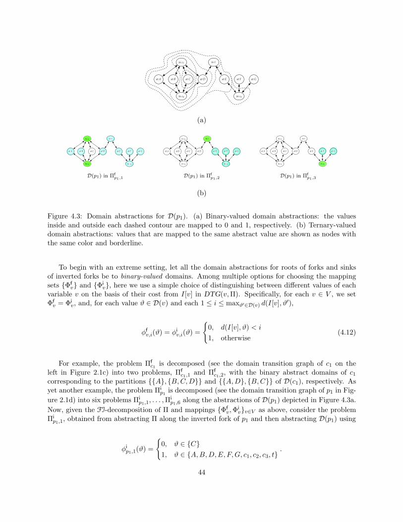
at A at B at C at D at E at F at G
in c₂
in c₁ in t
in c₃
(a)
at A at B at C at D at E at F at G
in c₂
in c₁ in t
in c₃
at A at B at C at D at E at F at G
in c₂
in c₁ in t
in c₃
at A at B at C at D at E at F at G
in c₂
in c₁ in t
in c₃
D(p1) in Πfp1,1
D(p1) in Πfp1,2
D(p1) in Πfp1,3
(b)
Figure 4.3: Domain abstractions for D(p1). (a) Binary-valued domain abstractions: the valuesinside and outside each dashed contour are mapped to 0 and 1, respectively. (b) Ternary-valueddomain abstractions: values that are mapped to the same abstract value are shown as nodes withthe same color and borderline.
To begin with an extreme setting, let all the domain abstractions for roots of forks and sinksof inverted forks be to binary-valued domains. Among multiple options for choosing the mappingsets {Φf
v} and {Φiv}, here we use a simple choice of distinguishing between different values of each
variable v on the basis of their cost from I[v] in DTG(v,Π). Specifically, for each v ∈ V , we setΦfv = Φi
v, and, for each value ϑ ∈ D(v) and each 1 ≤ i ≤ maxϑ′∈D(v) d(I[v], ϑ′),
φfv,i(ϑ) = φi
v,i(ϑ) =
{0, d(I[v], ϑ) < i
1, otherwise(4.12)
For example, the problem Πfc1 is decomposed (see the domain transition graph of c1 on the
left in Figure 2.1c) into two problems, Πfc1,1
and Πfc1,2
, with the binary abstract domains of c1
corresponding to the partitions {{A}, {B,C,D}} and {{A,D}, {B,C}} of D(c1), respectively. Asyet another example, the problem Πi
p1is decomposed (see the domain transition graph of p1 in Fig-
ure 2.1d) into six problems Πip1,1
, . . . ,Πip1,6
along the abstractions of D(p1) depicted in Figure 4.3a.Now, given the FI-decomposition of Π and mappings {Φf
v,Φiv}v∈V as above, consider the problem
Πip1,1
, obtained from abstracting Π along the inverted fork of p1 and then abstracting D(p1) using
φip1,1(ϑ) =
{0, ϑ ∈ {C}1, ϑ ∈ {A,B,D,E, F,G, c1, c2, c3, t}
.
44
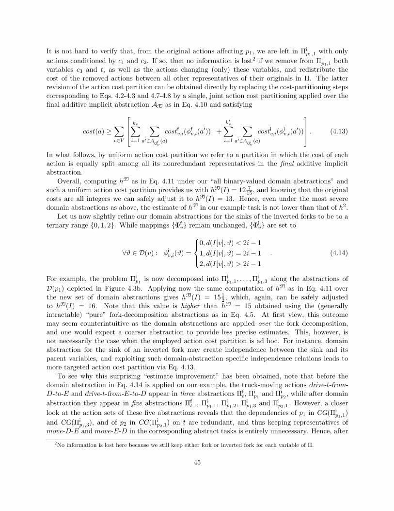
It is not hard to verify that, from the original actions affecting p1, we are left in Πip1,1
with onlyactions conditioned by c1 and c2. If so, then no information is lost2 if we remove from Πi
p1,1both
variables c3 and t, as well as the actions changing (only) these variables, and redistribute thecost of the removed actions between all other representatives of their originals in Π. The latterrevision of the action cost partition can be obtained directly by replacing the cost-partitioning stepscorresponding to Eqs. 4.2-4.3 and 4.7-4.8 by a single, joint action cost partitioning applied over thefinal additive implicit abstraction AFI as in Eq. 4.10 and satisfying
cost(a) ≥∑v∈V
kv∑i=1
∑a′∈AGf
v(a)
costfv,i(φfv,i(a
′)) +k′v∑i=1
∑a′∈AGi
v(a)
costiv,i(φiv,i(a
′))
. (4.13)
In what follows, by uniform action cost partition we refer to a partition in which the cost of eachaction is equally split among all its nonredundant representatives in the final additive implicitabstraction.
Overall, computing hFI as in Eq. 4.11 under our “all binary-valued domain abstractions” andsuch a uniform action cost partition provides us with hFI(I) = 12 7
15 , and knowing that the originalcosts are all integers we can safely adjust it to hFI(I) = 13. Hence, even under the most severedomain abstractions as above, the estimate of hFI in our example task is not lower than that of h2.
Let us now slightly refine our domain abstractions for the sinks of the inverted forks to be to aternary range {0, 1, 2}. While mappings {Φf
v} remain unchanged, {Φiv} are set to
∀ϑ ∈ D(v) : φiv,i(ϑ) =
0, d(I[v], ϑ) < 2i− 11, d(I[v], ϑ) = 2i− 12, d(I[v], ϑ) > 2i− 1
. (4.14)
For example, the problem Πip1
is now decomposed into Πip1,1
, . . . ,Πip1,3
along the abstractions ofD(p1) depicted in Figure 4.3b. Applying now the same computation of hFI as in Eq. 4.11 overthe new set of domain abstractions gives hFI(I) = 151
2 , which, again, can be safely adjustedto hFI(I) = 16. Note that this value is higher than hFI = 15 obtained using the (generallyintractable) “pure” fork-decomposition abstractions as in Eq. 4.5. At first view, this outcomemay seem counterintuitive as the domain abstractions are applied over the fork decomposition,and one would expect a coarser abstraction to provide less precise estimates. This, however, isnot necessarily the case when the employed action cost partition is ad hoc. For instance, domainabstraction for the sink of an inverted fork may create independence between the sink and itsparent variables, and exploiting such domain-abstraction specific independence relations leads tomore targeted action cost partition via Eq. 4.13.
To see why this surprising “estimate improvement” has been obtained, note that before thedomain abstraction in Eq. 4.14 is applied on our example, the truck-moving actions drive-t-from-D-to-E and drive-t-from-E-to-D appear in three abstractions Πf
t, Πip1
and Πip2
, while after domainabstraction they appear in five abstractions Πf
t,1, Πip1,1
, Πip1,2
, Πip1,3
and Πip2,1
. However, a closerlook at the action sets of these five abstractions reveals that the dependencies of p1 in CG(Πi
p1,1)
and CG(Πip1,3
), and of p2 in CG(Πip2,1
) on t are redundant, and thus keeping representatives ofmove-D-E and move-E-D in the corresponding abstract tasks is entirely unnecessary. Hence, after
2No information is lost here because we still keep either fork or inverted fork for each variable of Π.
45
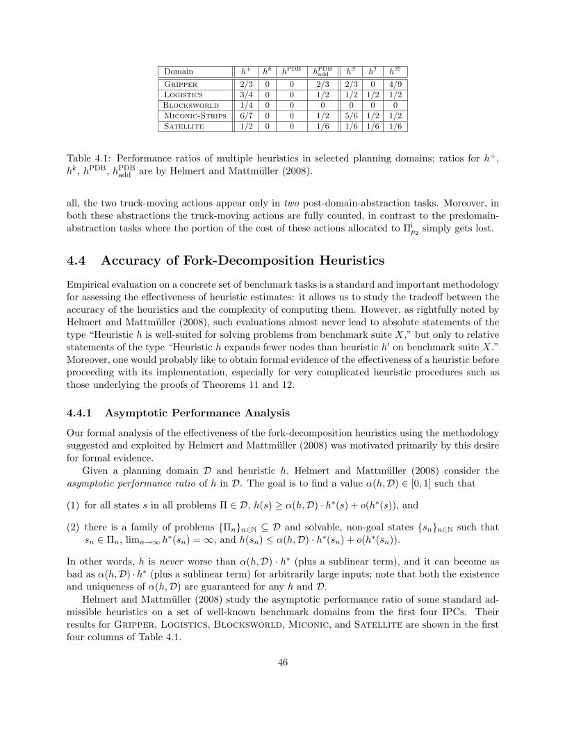
Domain h+ hk hPDB hPDBadd hF hI hFI
Gripper 2/3 0 0 2/3 2/3 0 4/9
Logistics 3/4 0 0 1/2 1/2 1/2 1/2
Blocksworld 1/4 0 0 0 0 0 0
Miconic-Strips 6/7 0 0 1/2 5/6 1/2 1/2
Satellite 1/2 0 0 1/6 1/6 1/6 1/6
Table 4.1: Performance ratios of multiple heuristics in selected planning domains; ratios for h+,hk, hPDB, hPDB
add are by Helmert and Mattmuller (2008).
all, the two truck-moving actions appear only in two post-domain-abstraction tasks. Moreover, inboth these abstractions the truck-moving actions are fully counted, in contrast to the predomain-abstraction tasks where the portion of the cost of these actions allocated to Πi
p2simply gets lost.
4.4 Accuracy of Fork-Decomposition Heuristics
Empirical evaluation on a concrete set of benchmark tasks is a standard and important methodologyfor assessing the effectiveness of heuristic estimates: it allows us to study the tradeoff between theaccuracy of the heuristics and the complexity of computing them. However, as rightfully noted byHelmert and Mattmuller (2008), such evaluations almost never lead to absolute statements of thetype “Heuristic h is well-suited for solving problems from benchmark suite X,” but only to relativestatements of the type “Heuristic h expands fewer nodes than heuristic h′ on benchmark suite X.”Moreover, one would probably like to obtain formal evidence of the effectiveness of a heuristic beforeproceeding with its implementation, especially for very complicated heuristic procedures such asthose underlying the proofs of Theorems 11 and 12.
4.4.1 Asymptotic Performance Analysis
Our formal analysis of the effectiveness of the fork-decomposition heuristics using the methodologysuggested and exploited by Helmert and Mattmuller (2008) was motivated primarily by this desirefor formal evidence.
Given a planning domain D and heuristic h, Helmert and Mattmuller (2008) consider theasymptotic performance ratio of h in D. The goal is to find a value α(h,D) ∈ [0, 1] such that
(1) for all states s in all problems Π ∈ D, h(s) ≥ α(h,D) · h∗(s) + o(h∗(s)), and
(2) there is a family of problems {Πn}n∈N ⊆ D and solvable, non-goal states {sn}n∈N such thatsn ∈ Πn, limn→∞ h
∗(sn) =∞, and h(sn) ≤ α(h,D) · h∗(sn) + o(h∗(sn)).
In other words, h is never worse than α(h,D) · h∗ (plus a sublinear term), and it can become asbad as α(h,D) ·h∗ (plus a sublinear term) for arbitrarily large inputs; note that both the existenceand uniqueness of α(h,D) are guaranteed for any h and D.
Helmert and Mattmuller (2008) study the asymptotic performance ratio of some standard ad-missible heuristics on a set of well-known benchmark domains from the first four IPCs. Theirresults for Gripper, Logistics, Blocksworld, Miconic, and Satellite are shown in the firstfour columns of Table 4.1.
46
• The h+ estimate corresponds to the optimal cost of solving the well-known “delete relaxation”of the original planning task, which is generally NP-hard to compute (Bylander, 1994).
• The hk, k ∈ N+, family of heuristics is based on a relaxation where the cost of achieving apartial assignment is approximated by the highest cost of achieving its sub-assignment of sizek (Haslum & Geffner, 2000); computing hk is exponential only in k.
• The hPDB and hPDBadd heuristics are regular (maximized over) and additive pattern database
heuristics where the size of each pattern is assumed to be O(log(n)) where n = |V |, and,importantly, the choice of the patterns is assumed to be optimal.
These results provide us with a baseline for evaluating our fork-decomposition heuristics hF, hI,and hFI. First, however, Theorem 10 shows that these three heuristics are worth analyzing becauseeach alone can be strictly more informative than the other two, depending on the planning taskand/or the state being evaluated.3
Theorem 10 (Undominance) Under uniform action cost partition, none of the heuristic func-tions hF, hI, and hFI dominates another.
Proof: The proof is by example of two tasks, Π1 and Π2, which illustrate the following twocases: hF(I) > hFI(I) > hI(I) and hF(I) < hFI(I) < hI(I). These two tasks are definedover the same set of binary-valued variables V = {v1, v2, v3, u1, u2, u3}, have the same initial stateI = {v1 =0, v2 =0, v3 =0, u1 =0, u2 =0, u3 =0}, and have the same goal G = {v1 =1, v2 =1, v3 =1}.The difference between Π1 and Π2 is in the action sets, listed in Figure 4.4c-d, with all the actionsbeing unit-cost actions. The two tasks induce identical causal graphs, depicted in Figure 4.4a.Hence, the collections of v-forks and v-iforks of both tasks are also identical; these are depicted inFigure 4.4b. The fractional costs of the tasks’ action representatives in the corresponding abstractproblems are given in Figure 4.4c-d.
Figure 4.5 shows the optimal plans for all the abstract problems in F-decompositions Π1F =
{Π1Gfu1
,Π1Gfu2
,Π1Gfu3
} and Π2F = {Π2
Gfu1
,Π2Gfu2
,Π2Gfu3
}, I-decompositions Π1I = {Π1
G iv1
,Π1G iv2
,Π1G iv3
} and
Π2I = {Π2
G iv1
,Π2G iv2
,Π2G iv3
}, and FI-decompositions Π1FI = Π1
F ∪Π1I and Π2
FI = Π2F ∪Π2
I . The last
column in both tables captures the estimates of the three heuristics for the initial states of Π1
and Π2, respectively. Together, these two cases show that none of the fork-decomposition heuristicfunctions hF, hI, and hFI dominates any other, and, since all the variables above are binary-valued,the claim holds in conjunction with arbitrary variable domain abstractions.
One conclusion from Theorem 10 is that it is worth studying the asymptotic performance ratiosfor all three heuristics. The last three columns of Table 4.1 present our results for hF, hI, and hFI
for the Gripper, Logistics, Blocksworld, Miconic, and Satellite domains. We also studiedthe performance ratios of max{hF, hI, hFI}, and in these five domains they appear to be identicalto those of hF. (Note that “ratio of max” should not necessarily be identical to “max of ratios,”and thus this analysis is worthwhile.) Taking a conservative position, the performance ratios forthe fork-decomposition heuristics in Table 4.1 are “worst-case” in the sense that
3Theorem 10 is formulated and proven under the uniform action cost partition that we use throughout this chapter,including the experiments. For per-step optimal action cost partitions (Katz & Domshlak, 2008b), it is trivial toshow that hFI dominates both hF and hI for all planning tasks.
47
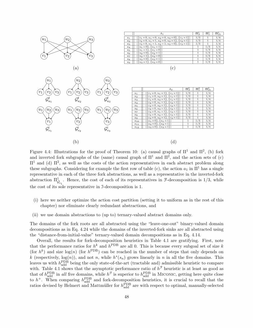
u1 u2 u3
v1 v2 v3
A1 Π1F Π1
I Π1FI
a1 〈{v1 =0, u1 =0, u2 =0, u3 =0}, {v1 =1}〉 1/3 1 1/4a2 〈{v2 =0, u1 =1, u2 =0, u3 =1}, {v2 =1}〉 1/3 1 1/4a3 〈{v3 =0, u1 =1, u2 =1, u3 =0}, {v3 =1}〉 1/3 1 1/4a4 〈{u1 =0}, {u1 =1}〉 1 1/3 1/4a5 〈{u1 =1}, {u1 =0}〉 1 1/3 1/4a6 〈{u2 =0}, {u2 =1}〉 1 1/3 1/4a7 〈{u2 =1}, {u2 =0}〉 1 1/3 1/4a8 〈{u3 =0}, {u3 =1}〉 1 1/3 1/4a9 〈{u3 =1}, {u3 =0}〉 1 1/3 1/4
(a) (c)
u1
v1 v2 v3
u2
v1 v2 v3
u3
v1 v2 v3
u1 u2 u3
v1
u1 u2 u3
v2
u1 u2 u3
v3
Gfu1
Gfu2
Gfu3
G iv1
G iv2
G iv3
A2 Π2F Π2
I Π2FI
a1 〈{v1 =0, u1 =1}, {v1 =1}〉 1/3 1 1/4a2 〈{v1 =0, u2 =1}, {v1 =1}〉 1/3 1 1/4a3 〈{v1 =0, u3 =1}, {v1 =1}〉 1/3 1 1/4a4 〈{v2 =0, u1 =1}, {v2 =1}〉 1/3 1 1/4a5 〈{v2 =0, u2 =1}, {v2 =1}〉 1/3 1 1/4a6 〈{v2 =0, u3 =1}, {v2 =1}〉 1/3 1 1/4a7 〈{v3 =0, u1 =1}, {v3 =1}〉 1/3 1 1/4a8 〈{v3 =0, u2 =1}, {v3 =1}〉 1/3 1 1/4a9 〈{v3 =0, u3 =1}, {v3 =1}〉 1/3 1 1/4a10 〈{u1 =0}, {u1 =1}〉 1 1/3 1/4a11 〈{u2 =0}, {u2 =1}〉 1 1/3 1/4a12 〈{u3 =0}, {u3 =1}〉 1 1/3 1/4
(b) (d)
Figure 4.4: Illustrations for the proof of Theorem 10: (a) causal graphs of Π1 and Π2, (b) forkand inverted fork subgraphs of the (same) causal graph of Π1 and Π2, and the action sets of (c)Π1 and (d) Π2, as well as the costs of the action representatives in each abstract problem alongthese subgraphs. Considering for example the first row of table (c), the action a1 in Π1 has a singlerepresentative in each of the three fork abstractions, as well as a representative in the inverted-forkabstraction Π1
G iv1
. Hence, the cost of each of its representatives in F-decomposition is 1/3, whilethe cost of its sole representative in I-decomposition is 1.
(i) here we neither optimize the action cost partition (setting it to uniform as in the rest of thischapter) nor eliminate clearly redundant abstractions, and
(ii) we use domain abstractions to (up to) ternary-valued abstract domains only.
The domains of the fork roots are all abstracted using the “leave-one-out” binary-valued domaindecompositions as in Eq. 4.24 while the domains of the inverted-fork sinks are all abstracted usingthe “distance-from-initial-value” ternary-valued domain decompositions as in Eq. 4.14.
Overall, the results for fork-decomposition heuristics in Table 4.1 are gratifying. First, notethat the performance ratios for hk and hPDB are all 0. This is because every subgoal set of size k(for hk) and size log(n) (for hPDB) can be reached in the number of steps that only depends onk (respectively, log(n)), and not n, while h∗(sn) grows linearly in n in all the five domains. Thisleaves us with hPDB
add being the only state-of-the-art (tractable and) admissible heuristic to comparewith. Table 4.1 shows that the asymptotic performance ratio of hF heuristic is at least as good asthat of hPDB
add in all five domains, while hF is superior to hPDBadd in Miconic, getting here quite close
to h+. When comparing hPDBadd and fork-decomposition heuristics, it is crucial to recall that the
ratios devised by Helmert and Mattmuller for hPDBadd are with respect to optimal, manually-selected
48
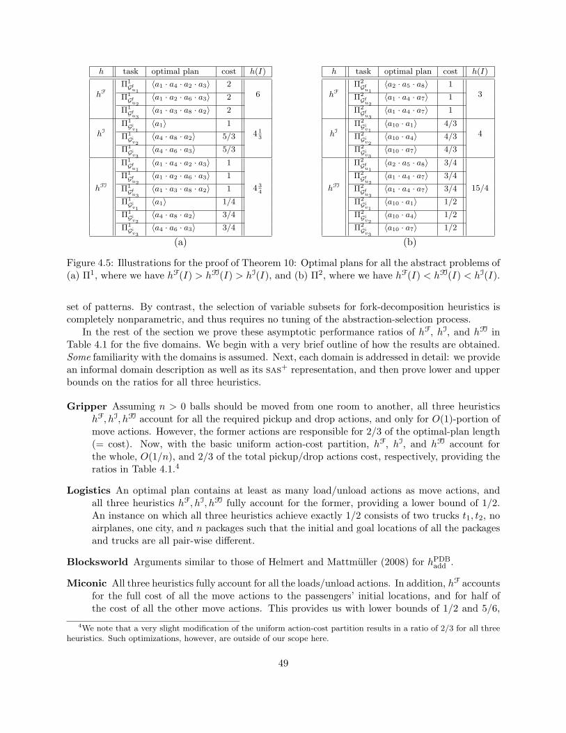
h task optimal plan cost h(I)
hFΠ1Gf
u1〈a1 · a4 · a2 · a3〉 2
6Π1Gf
u2〈a1 · a2 · a6 · a3〉 2
Π1Gf
u3〈a1 · a3 · a8 · a2〉 2
hIΠ1Gi
v1〈a1〉 1
4 13Π1
Giv2
〈a4 · a8 · a2〉 5/3
Π1Gi
v3〈a4 · a6 · a3〉 5/3
hFI
Π1Gf
u1〈a1 · a4 · a2 · a3〉 1
4 34
Π1Gf
u2〈a1 · a2 · a6 · a3〉 1
Π1Gf
u3〈a1 · a3 · a8 · a2〉 1
Π1Gi
v1〈a1〉 1/4
Π1Gi
v2〈a4 · a8 · a2〉 3/4
Π1Gi
v3〈a4 · a6 · a3〉 3/4
h task optimal plan cost h(I)
hFΠ2Gf
u1〈a2 · a5 · a8〉 1
3Π2Gf
u2〈a1 · a4 · a7〉 1
Π2Gf
u3〈a1 · a4 · a7〉 1
hIΠ2Gi
v1〈a10 · a1〉 4/3
4Π2Gi
v2〈a10 · a4〉 4/3
Π2Gi
v3〈a10 · a7〉 4/3
hFI
Π2Gf
u1〈a2 · a5 · a8〉 3/4
15/4
Π2Gf
u2〈a1 · a4 · a7〉 3/4
Π2Gf
u3〈a1 · a4 · a7〉 3/4
Π2Gi
v1〈a10 · a1〉 1/2
Π2Gi
v2〈a10 · a4〉 1/2
Π2Gi
v3〈a10 · a7〉 1/2
(a) (b)
Figure 4.5: Illustrations for the proof of Theorem 10: Optimal plans for all the abstract problems of(a) Π1, where we have hF(I) > hFI(I) > hI(I), and (b) Π2, where we have hF(I) < hFI(I) < hI(I).
set of patterns. By contrast, the selection of variable subsets for fork-decomposition heuristics iscompletely nonparametric, and thus requires no tuning of the abstraction-selection process.
In the rest of the section we prove these asymptotic performance ratios of hF, hI, and hFI inTable 4.1 for the five domains. We begin with a very brief outline of how the results are obtained.Some familiarity with the domains is assumed. Next, each domain is addressed in detail: we providean informal domain description as well as its sas+ representation, and then prove lower and upperbounds on the ratios for all three heuristics.
Gripper Assuming n > 0 balls should be moved from one room to another, all three heuristicshF, hI, hFI account for all the required pickup and drop actions, and only for O(1)-portion ofmove actions. However, the former actions are responsible for 2/3 of the optimal-plan length(= cost). Now, with the basic uniform action-cost partition, hF, hI, and hFI account forthe whole, O(1/n), and 2/3 of the total pickup/drop actions cost, respectively, providing theratios in Table 4.1.4
Logistics An optimal plan contains at least as many load/unload actions as move actions, andall three heuristics hF, hI, hFI fully account for the former, providing a lower bound of 1/2.An instance on which all three heuristics achieve exactly 1/2 consists of two trucks t1, t2, noairplanes, one city, and n packages such that the initial and goal locations of all the packagesand trucks are all pair-wise different.
Blocksworld Arguments similar to those of Helmert and Mattmuller (2008) for hPDBadd .
Miconic All three heuristics fully account for all the loads/unload actions. In addition, hF accountsfor the full cost of all the move actions to the passengers’ initial locations, and for half ofthe cost of all the other move actions. This provides us with lower bounds of 1/2 and 5/6,
4We note that a very slight modification of the uniform action-cost partition results in a ratio of 2/3 for all threeheuristics. Such optimizations, however, are outside of our scope here.
49
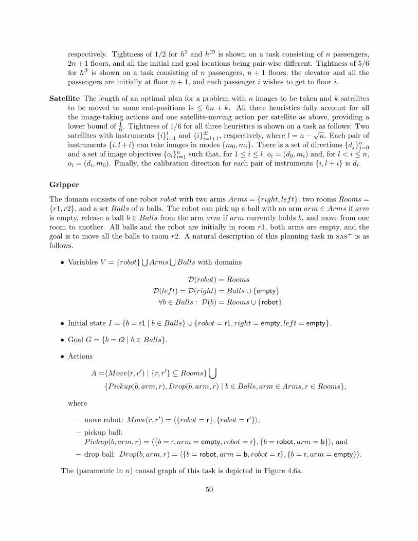
respectively. Tightness of 1/2 for hI and hFI is shown on a task consisting of n passengers,2n+ 1 floors, and all the initial and goal locations being pair-wise different. Tightness of 5/6for hF is shown on a task consisting of n passengers, n + 1 floors, the elevator and all thepassengers are initially at floor n+ 1, and each passenger i wishes to get to floor i.
Satellite The length of an optimal plan for a problem with n images to be taken and k satellitesto be moved to some end-positions is ≤ 6n + k. All three heuristics fully account for allthe image-taking actions and one satellite-moving action per satellite as above, providing alower bound of 1
6 . Tightness of 1/6 for all three heuristics is shown on a task as follows: Twosatellites with instruments {i}li=1 and {i}2li=l+1, respectively, where l = n−√n. Each pair ofinstruments {i, l+ i} can take images in modes {m0,mi}. There is a set of directions {dj}nj=0
and a set of image objectives {oi}ni=1 such that, for 1 ≤ i ≤ l, oi = (d0,mi) and, for l < i ≤ n,oi = (di,m0). Finally, the calibration direction for each pair of instruments {i, l + i} is di.
Gripper
The domain consists of one robot robot with two arms Arms = {right, left}, two rooms Rooms ={r1, r2}, and a set Balls of n balls. The robot can pick up a ball with an arm arm ∈ Arms if armis empty, release a ball b ∈ Balls from the arm arm if arm currently holds b, and move from oneroom to another. All balls and the robot are initially in room r1, both arms are empty, and thegoal is to move all the balls to room r2. A natural description of this planning task in sas+ is asfollows.
• Variables V = {robot}⋃Arms⋃Balls with domains
D(robot) = Rooms
D(left) = D(right) = Balls ∪ {empty}∀b ∈ Balls : D(b) = Rooms ∪ {robot}.
• Initial state I = {b = r1 | b ∈ Balls} ∪ {robot = r1, right = empty, left = empty}.
• Goal G = {b = r2 | b ∈ Balls}.
• Actions
A ={Move(r, r′) | {r, r′} ⊆ Rooms}⋃
{Pickup(b, arm, r), Drop(b, arm, r) | b ∈ Balls, arm ∈ Arms, r ∈ Rooms},
where
– move robot: Move(r, r′) = 〈{robot = r}, {robot = r′}〉,– pickup ball:Pickup(b, arm, r) = 〈{b = r, arm = empty, robot = r}, {b = robot, arm = b}〉, and
– drop ball: Drop(b, arm, r) = 〈{b = robot, arm = b, robot = r}, {b = r, arm = empty}〉.
The (parametric in n) causal graph of this task is depicted in Figure 4.6a.
50
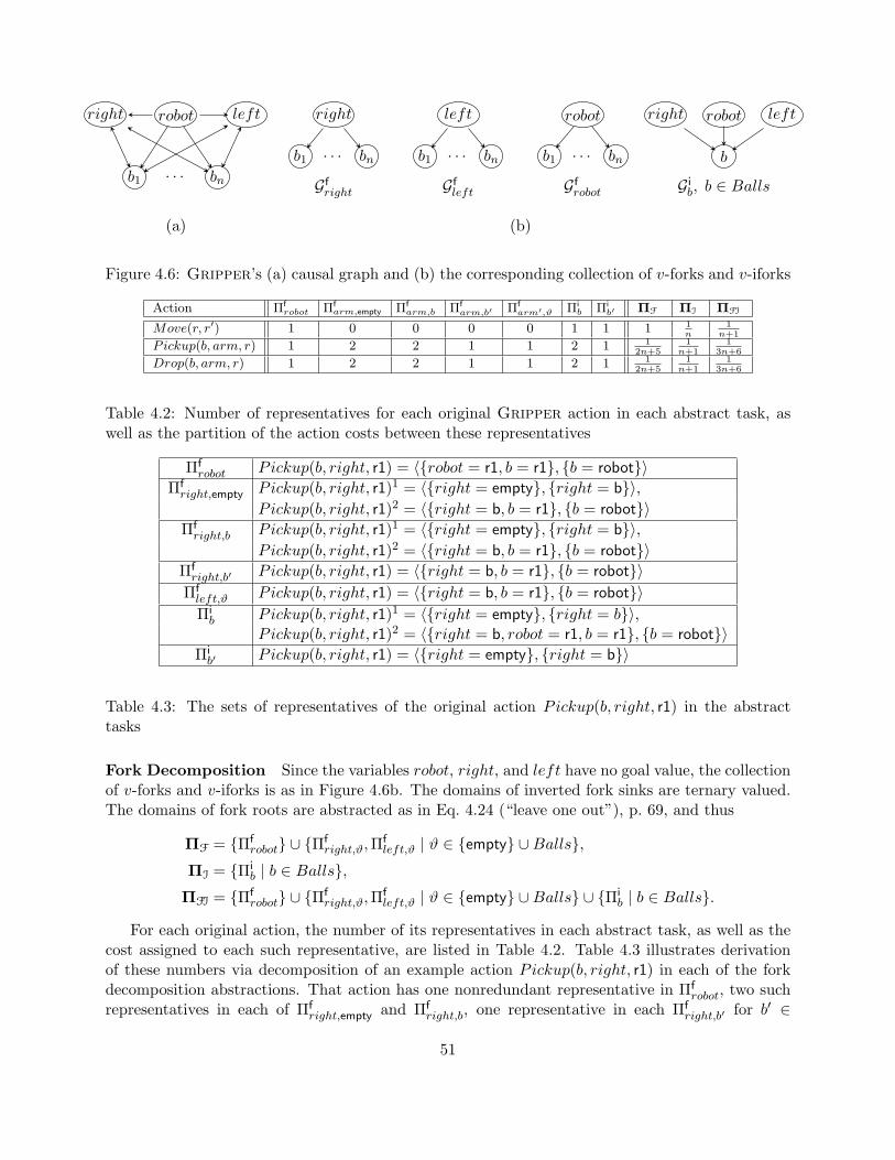
right robot left
b1 · · · bn
right
b1 . . . bn
left
b1 . . . bn
robot
b1 . . . bn
right robot left
b
Gfright Gf
left Gfrobot G i
b, b ∈ Balls
(a) (b)
Figure 4.6: Gripper’s (a) causal graph and (b) the corresponding collection of v-forks and v-iforks
Action Πfrobot Πf
arm,empty Πfarm,b Πf
arm,b′ Πfarm′,ϑ Πi
b Πib′ ΠF ΠI ΠFI
Move(r, r′) 1 0 0 0 0 1 1 1 1n
1n+1
Pickup(b, arm, r) 1 2 2 1 1 2 1 12n+5
1n+1
13n+6
Drop(b, arm, r) 1 2 2 1 1 2 1 12n+5
1n+1
13n+6
Table 4.2: Number of representatives for each original Gripper action in each abstract task, aswell as the partition of the action costs between these representatives
Πfrobot Pickup(b, right, r1) = 〈{robot = r1, b = r1}, {b = robot}〉
Πfright,empty Pickup(b, right, r1)1 = 〈{right = empty}, {right = b}〉,
Pickup(b, right, r1)2 = 〈{right = b, b = r1}, {b = robot}〉Πfright,b Pickup(b, right, r1)1 = 〈{right = empty}, {right = b}〉,
Pickup(b, right, r1)2 = 〈{right = b, b = r1}, {b = robot}〉Πfright,b′ Pickup(b, right, r1) = 〈{right = b, b = r1}, {b = robot}〉
Πfleft,ϑ Pickup(b, right, r1) = 〈{right = b, b = r1}, {b = robot}〉Πib Pickup(b, right, r1)1 = 〈{right = empty}, {right = b}〉,
Pickup(b, right, r1)2 = 〈{right = b, robot = r1, b = r1}, {b = robot}〉Πib′ Pickup(b, right, r1) = 〈{right = empty}, {right = b}〉
Table 4.3: The sets of representatives of the original action Pickup(b, right, r1) in the abstracttasks
Fork Decomposition Since the variables robot, right, and left have no goal value, the collectionof v-forks and v-iforks is as in Figure 4.6b. The domains of inverted fork sinks are ternary valued.The domains of fork roots are abstracted as in Eq. 4.24 (“leave one out”), p. 69, and thus
ΠF = {Πfrobot} ∪ {Πf
right,ϑ,Πfleft,ϑ | ϑ ∈ {empty} ∪Balls},
ΠI = {Πib | b ∈ Balls},
ΠFI = {Πfrobot} ∪ {Πf
right,ϑ,Πfleft,ϑ | ϑ ∈ {empty} ∪Balls} ∪ {Πi
b | b ∈ Balls}.
For each original action, the number of its representatives in each abstract task, as well as thecost assigned to each such representative, are listed in Table 4.2. Table 4.3 illustrates derivationof these numbers via decomposition of an example action Pickup(b, right, r1) in each of the forkdecomposition abstractions. That action has one nonredundant representative in Πf
robot, two suchrepresentatives in each of Πf
right,empty and Πfright,b, one representative in each Πf
right,b′ for b′ ∈
51
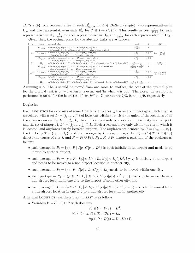
Balls \ {b}, one representative in each Πfleft,ϑ for ϑ ∈ Balls ∪ {empty}, two representatives in
Πib, and one representative in each Πi
b′ for b′ ∈ Balls \ {b}. This results in cost 12n+5 for each
representative in ΠF, 1n+1 for each representative in ΠI, and 1
3n+6 for each representative in ΠFI.Given that, the optimal plans for the abstract tasks are as follows.
h task optimal plan cost # h(I)
hF
Πfrobot 〈Pickup(b1, right, r1) · . . . · Pickup(bn, right, r1)· 4n+5
2n+5 1
2n− 2n−52n+5
·Move(r1, r2) ·Drop(b1, right, r2) · . . . ·Drop(bn, right, r2)〉Πf
right,ϑ 〈Pickup(b1, left, r1) · . . . · Pickup(bn, left, r1)· 2n2n+5 n + 1
·Drop(b1, left, r2) · . . . ·Drop(bn, left, r2)〉Πf
left,ϑ 〈Pickup(b1, right, r1) · . . . · Pickup(bn, right, r1)· 2n2n+5 n + 1
·Drop(b1, right, r2) · . . . ·Drop(bn, right, r2)〉hI Πi
b 〈Pickup(b, right, r1)1 · Pickup(b, right, r1)2 ·Move(r1, r2) ·Drop(b, left, r2)2〉 3n+1 + 1
nn 4n+1
n+1
hFI
Πfrobot 〈Pickup(b1, right, r1) · . . . · Pickup(bn, right, r1) ·Move(r1, r2)· 2n
3n+6 + 1n+1 1
4n3 + 4n+6
3n+6
·Drop(b1, right, r2) · . . . ·Drop(bn, right, r2)〉Πf
right,ϑ 〈Pickup(b1, left, r1) · . . . · Pickup(bn, left, r1)· 2n3n+6 n + 1
·Drop(b1, left, r2) · . . . ·Drop(bn, left, r2)〉Πf
left,ϑ 〈Pickup(b1, right, r1) · . . . · Pickup(bn, right, r1)· 2n3n+6 n + 1
·Drop(b1, right, r2) · . . . ·Drop(bn, right, r2)〉Πi
b 〈Pickup(b, right, r1)1 · Pickup(b, right, r1)2 ·Move(r1, r2) ·Drop(b, left, r2)2〉 33n+6 + 1
n+1 n
Assuming n > 0 balls should be moved from one room to another, the cost of the optimal planfor the original task is 3n − 1 when n is even, and 3n when n is odd. Therefore, the asymptoticperformance ratios for the heuristics hF, hI, hFI on Gripper are 2/3, 0, and 4/9, respectively.
Logistics
Each Logistics task consists of some k cities, x airplanes, y trucks and n packages. Each city i isassociated with a set Li = {l1i . . . , lαii } of locations within that city; the union of the locations of allthe cities is denoted by L =
⋃ki=1 Li. In addition, precisely one location in each city is an airport,
and the set of airports is LA = {l11 . . . , l1k} ⊆ L. Each truck can move only within the city in which itis located, and airplanes can fly between airports. The airplanes are denoted by U = {u1, . . . , ux},the trucks by T = {t1, . . . , ty}, and the packages by P = {p1, . . . , pn}. Let Ti = {t ∈ T | I[t] ∈ Li}denote the trucks of city i, and P = P1 ∪ P2 ∪ P3 ∪ P4 ∪ P5 denote a partition of the packages asfollows:
• each package in P1 = {p ∈ P | I[p], G[p] ∈ LA} is both initially at an airport and needs to bemoved to another airport,
• each package in P2 = {p ∈ P | I[p] ∈ LA ∩ Li, G[p] ∈ Lj \ LA, i 6= j} is initially at an airportand needs to be moved to a non-airport location in another city,
• each package in P3 = {p ∈ P | I[p] ∈ Li, G[p] ∈ Li} needs to be moved within one city,
• each package in P4 = {p ∈ P | I[p] ∈ Li \ LA, G[p] ∈ LA \ Li} needs to be moved from anon-airport location in one city to the airport of some other city, and
• each package in P5 = {p ∈ P | I[p] ∈ Li \ LA, G[p] ∈ Lj \ LA, i 6= j} needs to be moved froma non-airport location in one city to a non-airport location in another city.
A natural Logistics task description in sas+ is as follows.
• Variables V = U ∪ T ∪ P with domains∀u ∈ U : D(u) = LA,
∀1 ≤ i ≤ k, ∀t ∈ Ti : D(t) = Li,
∀p ∈ P : D(p) = L ∪ U ∪ T.
52
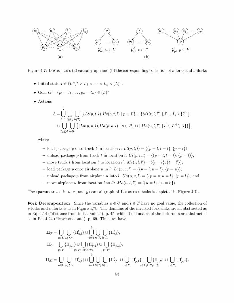
u1 · · · ux t1 · · · ty
p1 · · · pi · · · pn
u
p1 . . . pn
t
p1 . . . pn p
u1 . . . ux t1 . . . ty
Gfu, u ∈ U Gf
t , t ∈ T G ip, p ∈ P
(a) (b)
Figure 4.7: Logistics’s (a) causal graph and (b) the corresponding collection of v-forks and v-iforks
• Initial state I ∈ (LA)x × L1 × · · · × Lk × (L)n.
• Goal G = {p1 = l1, . . . , pn = ln} ∈ (L)n.
• Actions
A =k⋃i=1
⋃l∈Li
⋃t∈Ti
[{Lt(p, t, l), Ut(p, t, l) | p ∈ P} ∪ {Mt(t, l, l′) |, l′ ∈ Li \ {l}}
]∪⋃l∈LA
⋃u∈U
[{La(p, u, l), Ua(p, u, l) | p ∈ P} ∪ {Ma(u, l, l′) | l′ ∈ LA \ {l}}
],
where
– load package p onto truck t in location l: Lt(p, t, l) = 〈{p = l, t = l}, {p = t}〉,– unload package p from truck t in location l: Ut(p, t, l) = 〈{p = t, t = l}, {p = l}〉,– move truck t from location l to location l′: Mt(t, l, l′) = 〈{t = l}, {t = l′}〉,– load package p onto airplane u in l: La(p, u, l) = 〈{p = l, u = l}, {p = u}〉,– unload package p from airplane u into l: Ua(p, u, l) = 〈{p = u, u = l}, {p = l}〉, and
– move airplane u from location l to l′: Ma(u, l, l′) = 〈{u = l}, {u = l′}〉.
The (parametrized in n, x, and y) causal graph of Logistics tasks is depicted in Figure 4.7a.
Fork Decomposition Since the variables u ∈ U and t ∈ T have no goal value, the collection ofv-forks and v-iforks is as in Figure 4.7b. The domains of the inverted-fork sinks are all abstracted asin Eq. 4.14 (“distance-from-initial-value”), p. 45, while the domains of the fork roots are abstractedas in Eq. 4.24 (“leave-one-out”), p. 69. Thus, we have
ΠF =⋃u∈U
⋃l∈LA{Πf
u,l} ∪k⋃i=1
⋃t∈Ti
⋃l∈Li
{Πft,l},
ΠI =⋃p∈P{Πi
p,1} ∪⋃
p∈P2∪P4∪P5
{Πip,2} ∪
⋃p∈P5
{Πip,3},
ΠFI =⋃u∈U
⋃l∈LA{Πf
u,l} ∪k⋃i=1
⋃t∈Ti
⋃l∈Li
{Πft,l} ∪
⋃p∈P{Πi
p,1} ∪⋃
p∈P2∪P4∪P5
{Πip,2} ∪
⋃p∈P5
{Πip,3}.
53
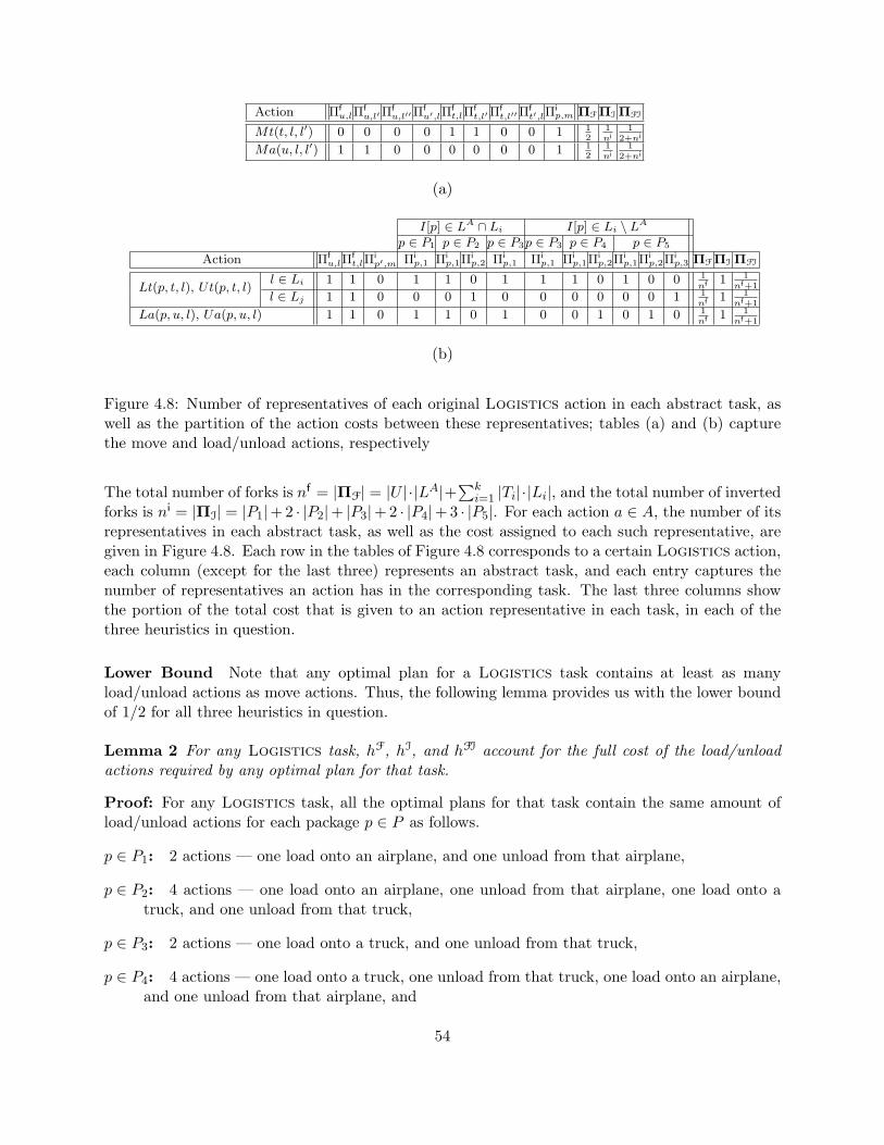
Action Πfu,lΠ
fu,l′Π
fu,l′′Π
fu′,lΠ
ft,lΠ
ft,l′Π
ft,l′′Π
ft′,lΠ
ip,m ΠFΠI ΠFI
Mt(t, l, l′) 0 0 0 0 1 1 0 0 1 12
1ni
12+ni
Ma(u, l, l′) 1 1 0 0 0 0 0 0 1 12
1ni
12+ni
(a)
I[p] ∈ LA ∩ Li I[p] ∈ Li \ LAp ∈ P1 p ∈ P2 p ∈ P3p ∈ P3 p ∈ P4 p ∈ P5
Action Πfu,lΠ
ft,lΠ
ip′,m Πi
p,1 Πip,1Πi
p,2 Πip,1 Πi
p,1 Πip,1Πi
p,2Πip,1Πi
p,2Πip,3 ΠFΠI ΠFI
Lt(p, t, l), Ut(p, t, l)l ∈ Li 1 1 0 1 1 0 1 1 1 0 1 0 0 1
nf 1 1nf+1
l ∈ Lj 1 1 0 0 0 1 0 0 0 0 0 0 1 1nf 1 1
nf+1
La(p, u, l), Ua(p, u, l) 1 1 0 1 1 0 1 0 0 1 0 1 0 1nf 1 1
nf+1
(b)
Figure 4.8: Number of representatives of each original Logistics action in each abstract task, aswell as the partition of the action costs between these representatives; tables (a) and (b) capturethe move and load/unload actions, respectively
The total number of forks is nf = |ΠF| = |U |·|LA|+∑k
i=1 |Ti|·|Li|, and the total number of invertedforks is ni = |ΠI| = |P1|+ 2 · |P2|+ |P3|+ 2 · |P4|+ 3 · |P5|. For each action a ∈ A, the number of itsrepresentatives in each abstract task, as well as the cost assigned to each such representative, aregiven in Figure 4.8. Each row in the tables of Figure 4.8 corresponds to a certain Logistics action,each column (except for the last three) represents an abstract task, and each entry captures thenumber of representatives an action has in the corresponding task. The last three columns showthe portion of the total cost that is given to an action representative in each task, in each of thethree heuristics in question.
Lower Bound Note that any optimal plan for a Logistics task contains at least as manyload/unload actions as move actions. Thus, the following lemma provides us with the lower boundof 1/2 for all three heuristics in question.
Lemma 2 For any Logistics task, hF, hI, and hFI account for the full cost of the load/unloadactions required by any optimal plan for that task.
Proof: For any Logistics task, all the optimal plans for that task contain the same amount ofload/unload actions for each package p ∈ P as follows.
p ∈ P1: 2 actions — one load onto an airplane, and one unload from that airplane,
p ∈ P2: 4 actions — one load onto an airplane, one unload from that airplane, one load onto atruck, and one unload from that truck,
p ∈ P3: 2 actions — one load onto a truck, and one unload from that truck,
p ∈ P4: 4 actions — one load onto a truck, one unload from that truck, one load onto an airplane,and one unload from that airplane, and
54
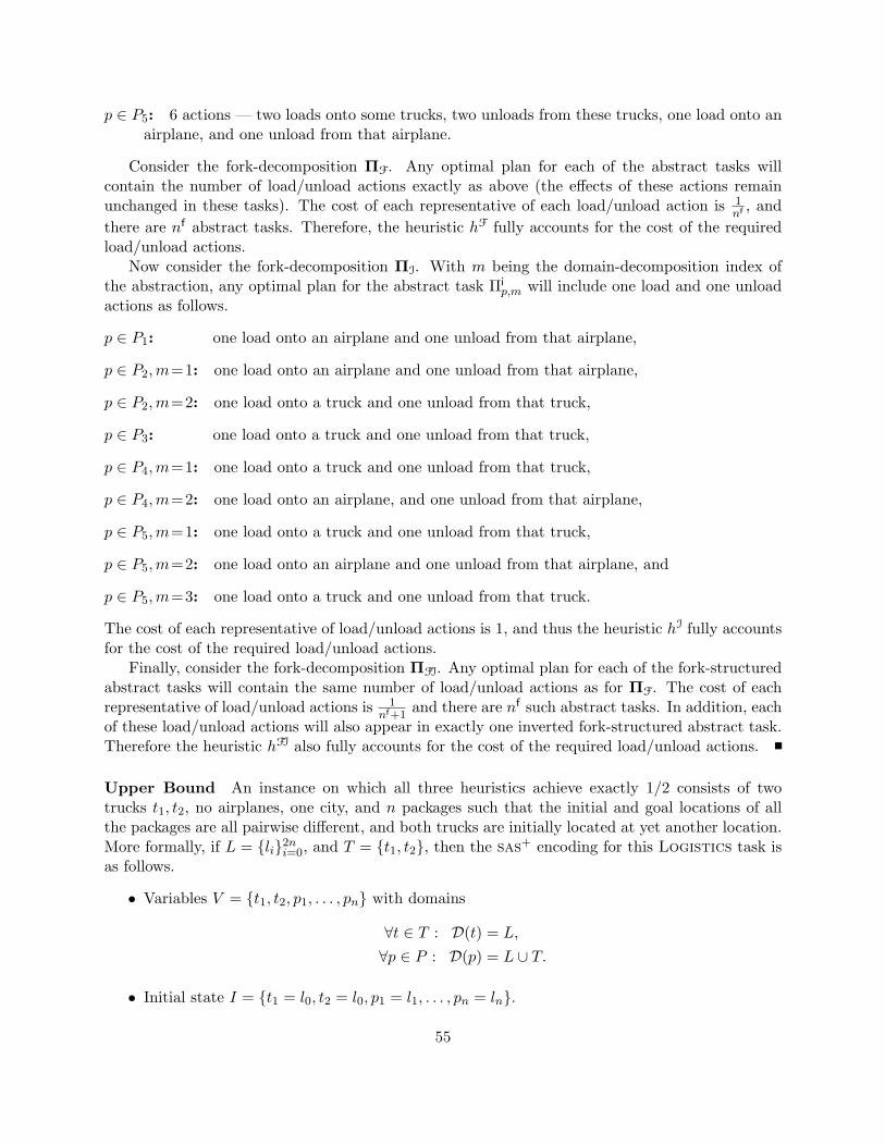
p ∈ P5: 6 actions — two loads onto some trucks, two unloads from these trucks, one load onto anairplane, and one unload from that airplane.
Consider the fork-decomposition ΠF. Any optimal plan for each of the abstract tasks willcontain the number of load/unload actions exactly as above (the effects of these actions remainunchanged in these tasks). The cost of each representative of each load/unload action is 1
nf , andthere are nf abstract tasks. Therefore, the heuristic hF fully accounts for the cost of the requiredload/unload actions.
Now consider the fork-decomposition ΠI. With m being the domain-decomposition index ofthe abstraction, any optimal plan for the abstract task Πi
p,m will include one load and one unloadactions as follows.
p ∈ P1: one load onto an airplane and one unload from that airplane,
p ∈ P2,m=1: one load onto an airplane and one unload from that airplane,
p ∈ P2,m=2: one load onto a truck and one unload from that truck,
p ∈ P3: one load onto a truck and one unload from that truck,
p ∈ P4,m=1: one load onto a truck and one unload from that truck,
p ∈ P4,m=2: one load onto an airplane, and one unload from that airplane,
p ∈ P5,m=1: one load onto a truck and one unload from that truck,
p ∈ P5,m=2: one load onto an airplane and one unload from that airplane, and
p ∈ P5,m=3: one load onto a truck and one unload from that truck.
The cost of each representative of load/unload actions is 1, and thus the heuristic hI fully accountsfor the cost of the required load/unload actions.
Finally, consider the fork-decomposition ΠFI. Any optimal plan for each of the fork-structuredabstract tasks will contain the same number of load/unload actions as for ΠF. The cost of eachrepresentative of load/unload actions is 1
nf+1and there are nf such abstract tasks. In addition, each
of these load/unload actions will also appear in exactly one inverted fork-structured abstract task.Therefore the heuristic hFI also fully accounts for the cost of the required load/unload actions.
Upper Bound An instance on which all three heuristics achieve exactly 1/2 consists of twotrucks t1, t2, no airplanes, one city, and n packages such that the initial and goal locations of allthe packages are all pairwise different, and both trucks are initially located at yet another location.More formally, if L = {li}2ni=0, and T = {t1, t2}, then the sas+ encoding for this Logistics task isas follows.
• Variables V = {t1, t2, p1, . . . , pn} with domains
∀t ∈ T : D(t) = L,
∀p ∈ P : D(p) = L ∪ T.
• Initial state I = {t1 = l0, t2 = l0, p1 = l1, . . . , pn = ln}.
55
t1
p1 . . . pn
t2
p1 . . . pn p
t1 t2
Gft1 Gf
t2 G ip, p ∈ P
Figure 4.9: Collection of v-forks and v-iforks for the Logistics task used for the proof of the upperbound of 1/2
• Goal G = {p1 = ln+1, . . . , pn = l2n}.
• Actions A = {Lt(p, t, l), Ut(p, t, l) | l ∈ L, t ∈ T, p ∈ P} ∪ {Mt(t, l, l′) | t ∈ T, {l, l′} ⊆ L}.
The collection of v-forks and v-iforks for this task is depicted in Figure 4.9. The domains ofthe inverted-fork sinks are all abstracted as in Eq. 4.14 (“distance-from-initial-value”), while thedomains of the fork roots are abstracted as in Eq. 4.24 (“leave-one-out”), and therefore we have
ΠF = {Πft1,lΠ
ft2,l | l ∈ L},
ΠI = {Πip,1 | p ∈ P},
ΠFI = {Πft1,lΠ
ft2,l | l ∈ L} ∪ {Πi
p,1 | p ∈ P}.
The total number of forks is thus nf = 4n+ 2 and the total number of inverted forks is ni = n. Thepartition of the action costs for Logistics tasks is described in Figure 4.8. Here we have P = P3
and thus the action cost partition is as follows.
Action Πft,l Πf
t,l′ Πft,l′′ Πf
t′,l∗ Πip,1 Πi
p′,1 ΠF ΠI ΠFI
Mt(t, l, l′) 1 1 0 0 1 0 12
1n
1n+2
Lt(p, t, l) 1 1 1 1 1 0 14n+2
1 14n+3
Ut(p, t, l) 1 1 1 1 1 0 14n+2
1 14n+3
Given that, the optimal plans for the abstract task are
h task optimal plan cost # h(I)
hF Πft1,l 〈Lt(p1, t2, l1) · . . . · Lt(pn, t2, ln) · Ut(p1, t2, ln+1) · . . . · Ut(pn, t2, l2n)〉 2n
4n+22n+ 1
2nΠft2,l 〈Lt(p1, t1, l1) · . . . · Lt(pn, t1, ln) · Ut(p1, t1, ln+1) · . . . · Ut(pn, t1, l2n)〉 2n
4n+22n+ 1
hI Πipi,1 〈Mt(t1, l0, li) · Lt(pi, t1, li) ·Mt(t1, li, ln+i) · Ut(pi, t1, ln+i)〉 2
n+ 2 n 2n+ 2
hFIΠft1,l 〈Lt(p1, t2, l1) · . . . · Lt(pn, t2, ln) · Ut(p1, t2, ln+1) · . . . · Ut(pn, t2, l2n)〉 2n
4n+32n+ 1
2n+ 2nn+2Πf
t2,l 〈Lt(p1, t1, l1) · . . . · Lt(pn, t1, ln) · Ut(p1, t1, ln+1) · . . . · Ut(pn, t1, l2n)〉 2n4n+3
2n+ 1
Πipi,1 〈Mt(t1, l0, li) · Lt(pi, t1, li) ·Mt(t1, li, ln+i) · Ut(pi, t1, ln+i)〉 2
n+2+ 2
4n+3n
while an optimal plan for the original task, e.g., 〈Mt(t1, l0, l1) · Lt(p1, t1, l1) ·Mt(t1, l1, l2) · Lt(p2, t1, l2) ·Mt(t1, l2, l3) · . . . ·Lt(pn, t1, ln) ·Mt(t1, ln, ln+1) ·Ut(p1, t1, ln+1) ·Mt(t1, ln+1, ln+2) ·Ut(p2, t1, ln+2) ·Mt(t1, ln+2, ln+3) ·. . .·Ut(pn, t1, l2n)〉, has the cost of 4n, providing us with the upper bound of 1/2 for all three heuristics.Putting our lower and upper bounds together, the asymptotic ratio of all three heuristics in questionis 1/2.
56
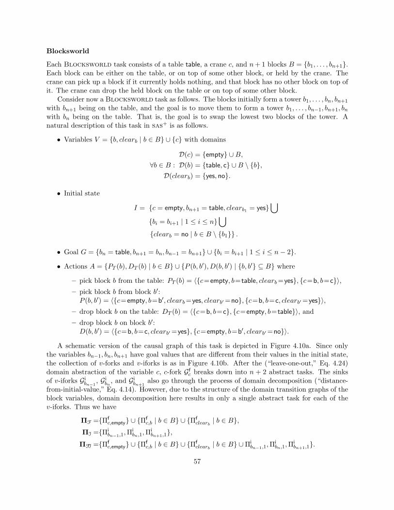
Blocksworld
Each Blocksworld task consists of a table table, a crane c, and n+ 1 blocks B = {b1, . . . , bn+1}.Each block can be either on the table, or on top of some other block, or held by the crane. Thecrane can pick up a block if it currently holds nothing, and that block has no other block on top ofit. The crane can drop the held block on the table or on top of some other block.
Consider now a Blocksworld task as follows. The blocks initially form a tower b1, . . . , bn, bn+1
with bn+1 being on the table, and the goal is to move them to form a tower b1, . . . , bn−1, bn+1, bnwith bn being on the table. That is, the goal is to swap the lowest two blocks of the tower. Anatural description of this task in sas+ is as follows.
• Variables V = {b, clearb | b ∈ B} ∪ {c} with domains
D(c) = {empty} ∪B,∀b ∈ B : D(b) = {table, c} ∪B \ {b},D(clearb) = {yes, no}.
• Initial state
I = {c = empty, bn+1 = table, clearb1 = yes}⋃
{bi = bi+1 | 1 ≤ i ≤ n}⋃
{clearb = no | b ∈ B \ {b1}} .
• Goal G = {bn = table, bn+1 = bn, bn−1 = bn+1} ∪ {bi = bi+1 | 1 ≤ i ≤ n− 2}.
• Actions A = {PT (b), DT (b) | b ∈ B} ∪ {P (b, b′), D(b, b′) | {b, b′} ⊆ B} where
– pick block b from the table: PT (b) = 〈{c=empty, b= table, clearb=yes}, {c=b, b=c}〉,– pick block b from block b′:P (b, b′) = 〈{c=empty, b=b′, clearb=yes, clearb′=no}, {c=b, b=c, clearb′=yes}〉,
– drop block b on the table: DT (b) = 〈{c=b, b=c}, {c=empty, b= table}〉, and
– drop block b on block b′:D(b, b′) = 〈{c=b, b=c, clearb′=yes}, {c=empty, b=b′, clearb′=no}〉.
A schematic version of the causal graph of this task is depicted in Figure 4.10a. Since onlythe variables bn−1, bn, bn+1 have goal values that are different from their values in the initial state,the collection of v-forks and v-iforks is as in Figure 4.10b. After the (“leave-one-out,” Eq. 4.24)domain abstraction of the variable c, c-fork Gf
c breaks down into n + 2 abstract tasks. The sinksof v-iforks G i
bn−1, G i
bn, and G i
bn+1also go through the process of domain decomposition (“distance-
from-initial-value,” Eq. 4.14). However, due to the structure of the domain transition graphs of theblock variables, domain decomposition here results in only a single abstract task for each of thev-iforks. Thus we have
ΠF ={Πfc,empty} ∪ {Πf
c,b | b ∈ B} ∪ {Πfclearb
| b ∈ B},ΠI ={Πi
bn−1,1,Πibn,1,Π
ibn+1,1},
ΠFI ={Πfc,empty} ∪ {Πf
c,b | b ∈ B} ∪ {Πfclearb
| b ∈ B} ∪Πibn−1,1,Π
ibn,1,Π
ibn+1,1}.
57
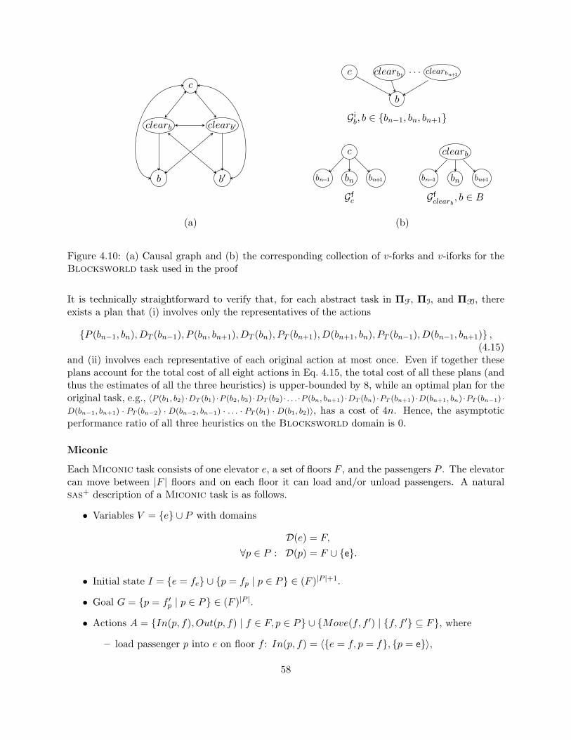
b b′
clearb clearb′
c
bn−1 bn bn+1
c
bn−1 bn bn+1
clearb
b
clearb1 . . . clearbn+1c
G ib, b ∈ {bn−1, bn, bn+1}
Gfc Gf
clearb, b ∈ B
(a) (b)
Figure 4.10: (a) Causal graph and (b) the corresponding collection of v-forks and v-iforks for theBlocksworld task used in the proof
It is technically straightforward to verify that, for each abstract task in ΠF, ΠI, and ΠFI, thereexists a plan that (i) involves only the representatives of the actions
{P (bn−1, bn), DT (bn−1), P (bn, bn+1), DT (bn), PT (bn+1), D(bn+1, bn), PT (bn−1), D(bn−1, bn+1)} ,(4.15)
and (ii) involves each representative of each original action at most once. Even if together theseplans account for the total cost of all eight actions in Eq. 4.15, the total cost of all these plans (andthus the estimates of all the three heuristics) is upper-bounded by 8, while an optimal plan for theoriginal task, e.g., 〈P (b1, b2) ·DT (b1) ·P (b2, b3) ·DT (b2) · . . . ·P (bn, bn+1) ·DT (bn) ·PT (bn+1) ·D(bn+1, bn) ·PT (bn−1) ·D(bn−1, bn+1) · PT (bn−2) · D(bn−2, bn−1) · . . . · PT (b1) · D(b1, b2)〉, has a cost of 4n. Hence, the asymptoticperformance ratio of all three heuristics on the Blocksworld domain is 0.
Miconic
Each Miconic task consists of one elevator e, a set of floors F , and the passengers P . The elevatorcan move between |F | floors and on each floor it can load and/or unload passengers. A naturalsas+ description of a Miconic task is as follows.
• Variables V = {e} ∪ P with domains
D(e) = F,
∀p ∈ P : D(p) = F ∪ {e}.
• Initial state I = {e = fe} ∪ {p = fp | p ∈ P} ∈ (F )|P |+1.
• Goal G = {p = f ′p | p ∈ P} ∈ (F )|P |.
• Actions A = {In(p, f), Out(p, f) | f ∈ F, p ∈ P} ∪ {Move(f, f ′) | {f, f ′} ⊆ F}, where
– load passenger p into e on floor f : In(p, f) = 〈{e = f, p = f}, {p = e}〉,
58
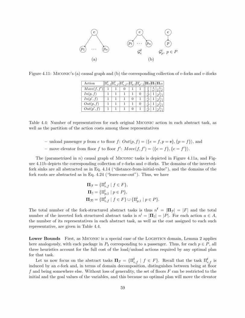
e
p1 · · · pn
e
p1 · · · pn
e
p
Gfe G i
p, p ∈ P(a) (b)
Figure 4.11: Miconic’s (a) causal graph and (b) the corresponding collection of v-forks and v-iforks
Action Πfe,fΠf
e,f ′Πfe,f ′′Π
ip,1Πi
p′,1 ΠFΠI ΠFI
Move(f, f ′) 1 1 0 1 1 12
1ni
12+ni
In(p, f) 1 1 1 1 0 1nf 1 1
nf+1
In(p′, f) 1 1 1 0 1 1nf 1 1
nf+1
Out(p, f) 1 1 1 1 0 1nf 1 1
nf+1
Out(p′, f) 1 1 1 0 1 1nf 1 1
nf+1
Table 4.4: Number of representatives for each original Miconic action in each abstract task, aswell as the partition of the action costs among these representatives
– unload passenger p from e to floor f : Out(p, f) = 〈{e = f, p = e}, {p = f}〉, and
– move elevator from floor f to floor f ′: Move(f, f ′) = 〈{e = f}, {e = f ′}〉.
The (parametrized in n) causal graph of Miconic tasks is depicted in Figure 4.11a, and Fig-ure 4.11b depicts the corresponding collection of v-forks and v-iforks. The domains of the inverted-fork sinks are all abstracted as in Eq. 4.14 (“distance-from-initial-value”), and the domains of thefork roots are abstracted as in Eq. 4.24 (“leave-one-out”). Thus, we have
ΠF = {Πfe,f | f ∈ F},
ΠI = {Πip,1 | p ∈ P},
ΠFI = {Πfe,f | f ∈ F} ∪ {Πi
p,1 | p ∈ P}.
The total number of the fork-structured abstract tasks is thus nf = |ΠF| = |F | and the totalnumber of the inverted fork structured abstract tasks is ni = |ΠI| = |P |. For each action a ∈ A,the number of its representatives in each abstract task, as well as the cost assigned to each suchrepresentative, are given in Table 4.4.
Lower Bounds First, as Miconic is a special case of the Logistics domain, Lemma 2 applieshere analogously, with each package in P3 corresponding to a passenger. Thus, for each p ∈ P , allthree heuristics account for the full cost of the load/unload actions required by any optimal planfor that task.
Let us now focus on the abstract tasks ΠF = {Πfe,f | f ∈ F}. Recall that the task Πf
e,f isinduced by an e-fork and, in terms of domain decomposition, distinguishes between being at floorf and being somewhere else. Without loss of generality, the set of floors F can be restricted to theinitial and the goal values of the variables, and this because no optimal plan will move the elevator
59
to or from a floor f that is neither an initial nor a goal location of a passenger or the elevator. LetFI = {I[p] | p ∈ P} and FG = {G[p] | p ∈ P}. The costs of the optimal plans for each abstract taskΠfe,f are as follows.
f ∈ FI ∩ FG : Let p, p′ ∈ P be a pair of passengers with initial and goal locations in f , respectively;that is, I[p] = G[p′] = f . If f = I[e], then any plan for Πf
e,f has to move the elevator fromf in order to load passenger p′, and then move the elevator back to f in order to unloadpassenger p′. Therefore the cost of any plan for Πf
e,f is at least 2|P ||F | + 1, where (see the last
three columns of Table 4.4) the first component of the summation comes from summing thecosts of the representatives of the load/unload actions for all the passengers, and the secondcomponent is the sum of the costs of representatives of the two respective move actions.Similarly, if f 6= I[e], then any plan for Πf
e,f has to move the elevator to f in order to loadpassenger p, and then move the elevator from f in order to unload p. Therefore, here as well,the cost of any plan for Πf
e,f is at least 2|P ||F | + 1.
f ∈ FI \ FG : Let p ∈ P be a passenger initially at f , that is, I[p] = f . If f = I[e], then any planfor Πf
e,f has to move the elevator from f in order to unload p, and thus the cost of any plan
for Πfe,f is at least 2|P |
|F | + 12 . Otherwise, if f 6= I[e], then any plan for Πf
e,f has to move theelevator to f in order to load p, and then move the elevator from f in order to unload p.Hence, in this case, the cost of any plan for Πf
e,f is at least 2|P ||F | + 1.
f ∈ FG \ FI : Let p ∈ P be a passenger who must arrive at floor f , that is, G[p] = f . If f = I[e],then any plan for Πf
e,f has to move the elevator from f in order to load p, and then move theelevator back to f in order to unload p. Hence, here as well, the cost of any plan for Πf
e,f is
at least 2|P ||F | + 1. Otherwise, if f 6= I[e], then any plan for Πf
e,f has to move the elevator to f
in order to unload p, and thus the cost of any plan for Πfe,f is at least 2|P |
|F | + 12 .
f 6∈ FG ∪ FI : If f = I[e], then any plan for Πfe,f has to include a move from f in order to
load/unload the passengers, and thus the cost of any plan for Πfe,f is at least 2|P |
|F | + 12 .
Otherwise, if f 6= I[e], the elevator is initially “in the set of all other locations,” and thus thecost of any plan for Πf
e,f is at least 2|P ||F | .
Putting this case-by-case analysis together, we have
hF(I) ≥
2|P |+ |FI ∩ FG|+ |FI \ FG|+ |FG\FI |
2 , I[e] ∈ FI ∩ FG2|P |+ |FI ∩ FG|+ |FI \ FG| − 1 + 1
2 + |FG\FI |2 , I[e] ∈ FI \ FG
2|P |+ |FI ∩ FG|+ |FI \ FG|+ 1 + |FG\FI |−12 , I[e] ∈ FG \ FI
2|P |+ |FI ∩ FG|+ |FI \ FG|+ |FG\FI |−12 + 1
2 , I[e] 6∈ FG ∪ FI
.
Note that the value in the second case is the lowest. This gives us a lower bound on the hF estimateas in Eq. 4.16.
hF(I) ≥ 2|P |+ |FI \ FG|+|FG \ FI |
2+ |FI ∩ FG| −
12. (4.16)
Now, let us provide an upper bound on the length (= cost) of the optimal plan for a Miconictask. First, let P ′ ⊆ P denote the set of passengers with both initial and goal locations in FI ∩FG.
60
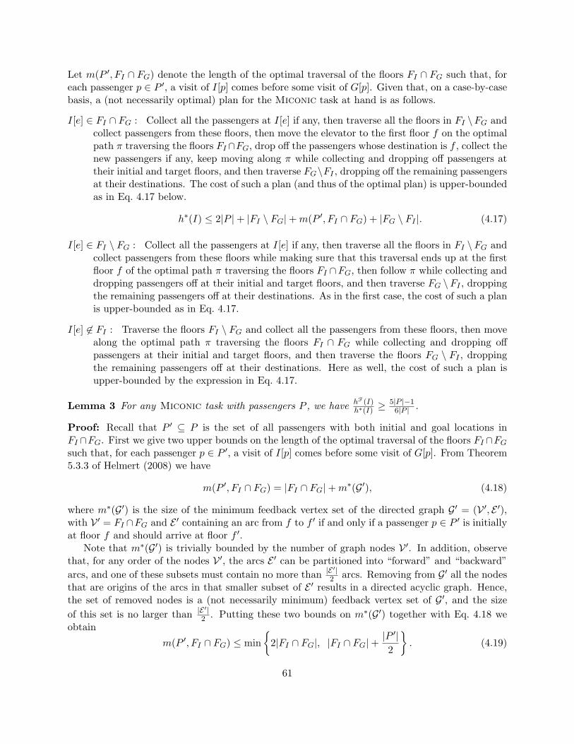
Let m(P ′, FI ∩ FG) denote the length of the optimal traversal of the floors FI ∩ FG such that, foreach passenger p ∈ P ′, a visit of I[p] comes before some visit of G[p]. Given that, on a case-by-casebasis, a (not necessarily optimal) plan for the Miconic task at hand is as follows.
I[e] ∈ FI ∩ FG : Collect all the passengers at I[e] if any, then traverse all the floors in FI \FG andcollect passengers from these floors, then move the elevator to the first floor f on the optimalpath π traversing the floors FI∩FG, drop off the passengers whose destination is f , collect thenew passengers if any, keep moving along π while collecting and dropping off passengers attheir initial and target floors, and then traverse FG\FI , dropping off the remaining passengersat their destinations. The cost of such a plan (and thus of the optimal plan) is upper-boundedas in Eq. 4.17 below.
h∗(I) ≤ 2|P |+ |FI \ FG|+m(P ′, FI ∩ FG) + |FG \ FI |. (4.17)
I[e] ∈ FI \ FG : Collect all the passengers at I[e] if any, then traverse all the floors in FI \FG andcollect passengers from these floors while making sure that this traversal ends up at the firstfloor f of the optimal path π traversing the floors FI ∩FG, then follow π while collecting anddropping passengers off at their initial and target floors, and then traverse FG \FI , droppingthe remaining passengers off at their destinations. As in the first case, the cost of such a planis upper-bounded as in Eq. 4.17.
I[e] 6∈ FI : Traverse the floors FI \ FG and collect all the passengers from these floors, then movealong the optimal path π traversing the floors FI ∩ FG while collecting and dropping offpassengers at their initial and target floors, and then traverse the floors FG \ FI , droppingthe remaining passengers off at their destinations. Here as well, the cost of such a plan isupper-bounded by the expression in Eq. 4.17.
Lemma 3 For any Miconic task with passengers P , we have hF(I)h∗(I) ≥
5|P |−16|P | .
Proof: Recall that P ′ ⊆ P is the set of all passengers with both initial and goal locations inFI ∩FG. First we give two upper bounds on the length of the optimal traversal of the floors FI ∩FGsuch that, for each passenger p ∈ P ′, a visit of I[p] comes before some visit of G[p]. From Theorem5.3.3 of Helmert (2008) we have
m(P ′, FI ∩ FG) = |FI ∩ FG|+m∗(G′), (4.18)
where m∗(G′) is the size of the minimum feedback vertex set of the directed graph G′ = (V ′, E ′),with V ′ = FI ∩FG and E ′ containing an arc from f to f ′ if and only if a passenger p ∈ P ′ is initiallyat floor f and should arrive at floor f ′.
Note that m∗(G′) is trivially bounded by the number of graph nodes V ′. In addition, observethat, for any order of the nodes V ′, the arcs E ′ can be partitioned into “forward” and “backward”arcs, and one of these subsets must contain no more than |E
′|2 arcs. Removing from G′ all the nodes
that are origins of the arcs in that smaller subset of E ′ results in a directed acyclic graph. Hence,the set of removed nodes is a (not necessarily minimum) feedback vertex set of G′, and the sizeof this set is no larger than |E ′|
2 . Putting these two bounds on m∗(G′) together with Eq. 4.18 weobtain
m(P ′, FI ∩ FG) ≤ min{
2|FI ∩ FG|, |FI ∩ FG|+|P ′|2
}. (4.19)
61
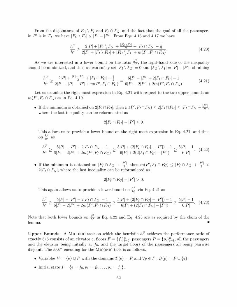
From the disjointness of FG \ FI and FI ∩ FG, and the fact that the goal of all the passengersin P ′ is in FI , we have |FG \ FI | ≤ |P | − |P ′|. From Eqs. 4.16 and 4.17 we have
hF
h∗≥ 2|P |+ |FI \ FG|+ |FG\FI |
2 + |FI ∩ FG| − 12
2|P |+ |FI \ FG|+ |FG \ FI |+m(P ′, FI ∩ FG). (4.20)
As we are interested in a lower bound on the ratio hF
h∗ , the right-hand side of the inequalityshould be minimized, and thus we can safely set |FI \FG| = 0 and |FG \FI | = |P | − |P ′|, obtaining
hF
h∗≥ 2|P |+ |P |−|P ′|
2 + |FI ∩ FG| − 12
2|P |+ |P | − |P ′|+m(P ′, FI ∩ FG)=
5|P | − |P ′|+ 2|FI ∩ FG| − 16|P | − 2|P ′|+ 2m(P ′, FI ∩ FG)
. (4.21)
Let us examine the right-most expression in Eq. 4.21 with respect to the two upper bounds onm(P ′, FI ∩ FG) as in Eq. 4.19.
• If the minimum is obtained on 2|FI ∩FG|, then m(P ′, FI ∩FG) ≤ 2|FI ∩FG| ≤ |FI ∩FG|+ |P′|
2 ,where the last inequality can be reformulated as
2|FI ∩ FG| − |P ′| ≤ 0.
This allows us to provide a lower bound on the right-most expression in Eq. 4.21, and thuson hF
h∗ as
hF
h∗≥ 5|P | − |P ′|+ 2|FI ∩ FG| − 1
6|P | − 2|P ′|+ 2m(P ′, FI ∩ FG)≥ 5|P |+ (2|FI ∩ FG| − |P ′|)− 1
6|P |+ 2(2|FI ∩ FG| − |P ′|)≥ 5|P | − 1
6|P | . (4.22)
• If the minimum is obtained on |FI ∩ FG| + |P ′|2 , then m(P ′, FI ∩ FG) ≤ |FI ∩ FG| + |P ′|
2 <2|FI ∩ FG|, where the last inequality can be reformulated as
2|FI ∩ FG| − |P ′| > 0.
This again allows us to provide a lower bound on hF
h∗ via Eq. 4.21 as
hF
h∗≥ 5|P | − |P ′|+ 2|FI ∩ FG| − 1
6|P | − 2|P ′|+ 2m(P ′, FI ∩ FG)≥ 5|P |+ (2|FI ∩ FG| − |P ′|)− 1
6|P |+ (2|FI ∩ FG| − |P ′|)≥ 5|P | − 1
6|P | . (4.23)
Note that both lower bounds on hF
h∗ in Eq. 4.22 and Eq. 4.23 are as required by the claim of thelemma.
Upper Bounds A Miconic task on which the heuristic hF achieves the performance ratio ofexactly 5/6 consists of an elevator e, floors F = {fi}ni=0, passengers P = {pi}ni=1, all the passengersand the elevator being initially at f0, and the target floors of the passengers all being pairwisedisjoint. The sas+ encoding for the Miconic task is as follows.
• Variables V = {e} ∪ P with the domains D(e) = F and ∀p ∈ P : D(p) = F ∪ {e}.
• Initial state I = {e = f0, p1 = f0, . . . , pn = f0}.
62
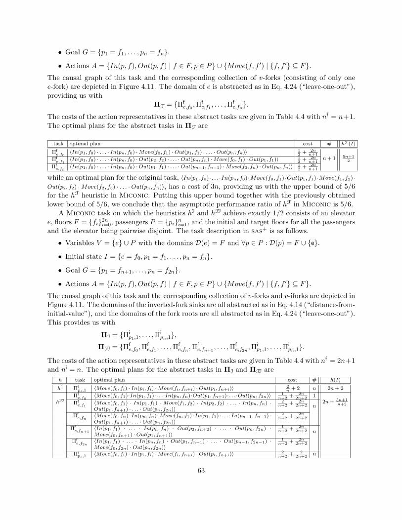
• Goal G = {p1 = f1, . . . , pn = fn}.• Actions A = {In(p, f), Out(p, f) | f ∈ F, p ∈ P} ∪ {Move(f, f ′) | {f, f ′} ⊆ F}.
The causal graph of this task and the corresponding collection of v-forks (consisting of only onee-fork) are depicted in Figure 4.11. The domain of e is abstracted as in Eq. 4.24 (“leave-one-out”),providing us with
ΠF = {Πfe,f0
,Πfe,f1
, . . . ,Πfe,fn}.
The costs of the action representatives in these abstract tasks are given in Table 4.4 with nf = n+1.The optimal plans for the abstract tasks in ΠF are
task optimal plan cost # hF(I)
Πfe,f0
〈In(p1, f0) · . . . · In(pn, f0) ·Move(f0, f1) ·Out(p1, f1) · . . . ·Out(pn, fn)〉 12
+ 2nn+1
n+ 1 5n+12Πf
e,f1〈In(p1, f0) · . . . · In(pn, f0) ·Out(p2, f2) · . . . ·Out(pn, fn) ·Move(f0, f1) ·Out(p1, f1)〉 1
2+ 2nn+1
Πfe,fn
〈In(p1, f0) · . . . · In(pn, f0) ·Out(p1, f1) · . . . ·Out(pn−1, fn−1) ·Move(f0, fn) ·Out(pn, fn)〉 12
+ 2nn+1
while an optimal plan for the original task, 〈In(p1, f0)·. . .·In(pn, f0)·Move(f0, f1)·Out(p1, f1)·Move(f1, f2)·Out(p2, f2) ·Move(f2, f3) · . . . · Out(pn, fn)〉, has a cost of 3n, providing us with the upper bound of 5/6for the hF heuristic in Miconic. Putting this upper bound together with the previously obtainedlower bound of 5/6, we conclude that the asymptotic performance ratio of hF in Miconic is 5/6.
A Miconic task on which the heuristics hI and hFI achieve exactly 1/2 consists of an elevatore, floors F = {fi}2ni=0, passengers P = {pi}ni=1, and the initial and target floors for all the passengersand the elevator being pairwise disjoint. The task description in sas+ is as follows.
• Variables V = {e} ∪ P with the domains D(e) = F and ∀p ∈ P : D(p) = F ∪ {e}.• Initial state I = {e = f0, p1 = f1, . . . , pn = fn}.• Goal G = {p1 = fn+1, . . . , pn = f2n}.• Actions A = {In(p, f), Out(p, f) | f ∈ F, p ∈ P} ∪ {Move(f, f ′) | {f, f ′} ⊆ F}.
The causal graph of this task and the corresponding collection of v-forks and v-iforks are depicted inFigure 4.11. The domains of the inverted-fork sinks are all abstracted as in Eq. 4.14 (“distance-from-initial-value”), and the domains of the fork roots are all abstracted as in Eq. 4.24 (“leave-one-out”).This provides us with
ΠI = {Πip1,1, . . . ,Π
ipn,1},
ΠFI = {Πfe,f0
,Πfe,f1
, . . . ,Πfe,fn ,Π
fe,fn+1
, . . . ,Πfe,f2n
,Πip1,1, . . . ,Π
ipn,1}.
The costs of the action representatives in these abstract tasks are given in Table 4.4 with nf = 2n+1and ni = n. The optimal plans for the abstract tasks in ΠI and ΠFI are
h task optimal plan cost # h(I)
hI Πipi,1
〈Move(f0, fi) · In(pi, fi) ·Move(fi, fn+i) ·Out(pi, fn+i)〉 2n
+ 2 n 2n+ 2
hFIΠfe,f0
〈Move(f0, f1)·In(p1, f1)·. . .·In(pn, fn)·Out(p1, fn+1)·. . .·Out(pn, f2n)〉 1n+2
+ 2n2n+2
12n+ 5n+1
n+2Πfe,f1
〈Move(f0, f1) · In(p1, f1) · Move(f1, f2) · In(p2, f2) · . . . · In(pn, fn) ·Out(p1, fn+1) · . . . ·Out(pn, f2n)〉
2n+2
+ 2n2n+2 n
Πfe,fn
〈Move(f0, fn) ·In(pn, fn) ·Move(fn, f1) ·In(p1, f1) · . . . ·In(pn−1, fn−1) ·Out(p1, fn+1) · . . . ·Out(pn, f2n)〉
2n+2
+ 2n2n+2
Πfe,fn+1
〈In(p1, f1) · . . . · In(pn, fn) · Out(p2, fn+2) · . . . · Out(pn, f2n) ·Move(f0, fn+1) ·Out(p1, fn+1)〉
1n+2
+ 2n2n+2 n
Πfe,f2n
〈In(p1, f1) · . . . · In(pn, fn) · Out(p1, fn+1) · . . . · Out(pn−1, f2n−1) ·Move(f0, f2n) ·Out(pn, f2n)〉
1n+2
+ 2n2n+2
Πipi,1
〈Move(f0, fi) · In(pi, fi) ·Move(fi, fn+i) ·Out(pi, fn+i)〉 2n+2
+ 22n+2
n
63
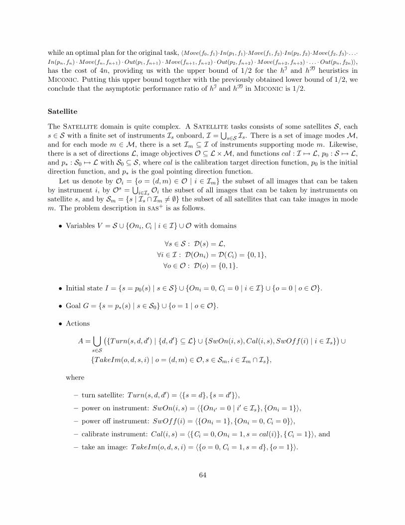
while an optimal plan for the original task, 〈Move(f0, f1)·In(p1, f1)·Move(f1, f2)·In(p2, f2)·Move(f2, f3)·. . .·In(pn, fn) ·Move(fn, fn+1) ·Out(p1, fn+1) ·Move(fn+1, fn+2) ·Out(p2, fn+2) ·Move(fn+2, fn+3) · . . . ·Out(pn, f2n)〉,has the cost of 4n, providing us with the upper bound of 1/2 for the hI and hFI heuristics inMiconic. Putting this upper bound together with the previously obtained lower bound of 1/2, weconclude that the asymptotic performance ratio of hI and hFI in Miconic is 1/2.
Satellite
The Satellite domain is quite complex. A Satellite tasks consists of some satellites S, eachs ∈ S with a finite set of instruments Is onboard, I =
⋃s∈S Is. There is a set of image modes M,
and for each mode m ∈ M, there is a set Im ⊆ I of instruments supporting mode m. Likewise,there is a set of directions L, image objectives O ⊆ L×M, and functions cal : I 7→ L, p0 : S 7→ L,and p∗ : S0 7→ L with S0 ⊆ S, where cal is the calibration target direction function, p0 is the initialdirection function, and p∗ is the goal pointing direction function.
Let us denote by Oi = {o = (d,m) ∈ O | i ∈ Im} the subset of all images that can be takenby instrument i, by Os =
⋃i∈Is Oi the subset of all images that can be taken by instruments on
satellite s, and by Sm = {s | Is ∩ Im 6= ∅} the subset of all satellites that can take images in modem. The problem description in sas+ is as follows.
• Variables V = S ∪ {Oni,Ci | i ∈ I} ∪ O with domains
∀s ∈ S : D(s) = L,∀i ∈ I : D(Oni) = D(Ci) = {0, 1},∀o ∈ O : D(o) = {0, 1}.
• Initial state I = {s = p0(s) | s ∈ S} ∪ {Oni = 0,Ci = 0 | i ∈ I} ∪ {o = 0 | o ∈ O}.
• Goal G = {s = p∗(s) | s ∈ S0} ∪ {o = 1 | o ∈ O}.
• Actions
A =⋃s∈S
({Turn(s, d, d′) | {d, d′} ⊆ L} ∪ {SwOn(i, s), Cal(i, s), SwOff(i) | i ∈ Is}
)∪
{TakeIm(o, d, s, i) | o = (d,m) ∈ O, s ∈ Sm, i ∈ Im ∩ Is},
where
– turn satellite: Turn(s, d, d′) = 〈{s = d}, {s = d′}〉,– power on instrument: SwOn(i, s) = 〈{Oni′ = 0 | i′ ∈ Is}, {Oni = 1}〉,– power off instrument: SwOff(i) = 〈{Oni = 1}, {Oni = 0,Ci = 0}〉,– calibrate instrument: Cal(i, s) = 〈{Ci = 0, Oni = 1, s = cal(i)}, {Ci = 1}〉, and
– take an image: TakeIm(o, d, s, i) = 〈{o = 0,Ci = 1, s = d}, {o = 1}〉.
64
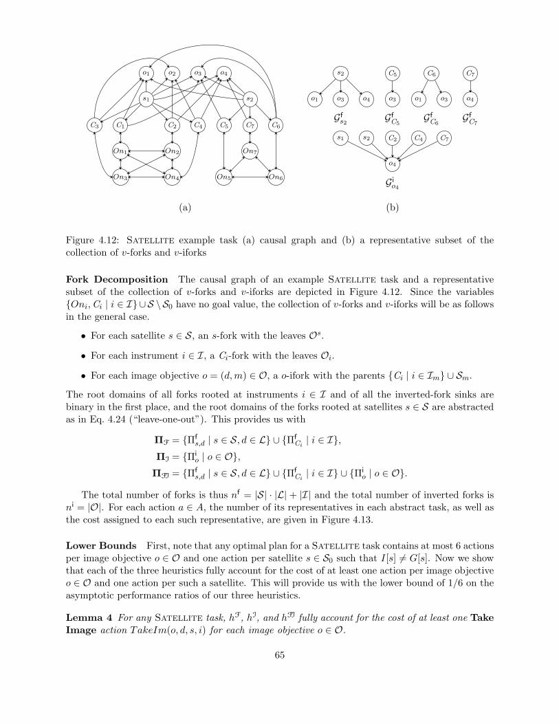
o1 o2 o3 o4
s1 s2
C1 C2C3 C4 C5 C6C7
On1 On2
On3 On4 On5 On6
On7
o1 o3 o4
s2
o3
C5
o1 o3
C6
o4
C7
o4
s1 s2 C2 C4 C7
(a) (b)
Gfs2 Gf
C5Gf
C6Gf
C7
G io4
Figure 4.12: Satellite example task (a) causal graph and (b) a representative subset of thecollection of v-forks and v-iforks
Fork Decomposition The causal graph of an example Satellite task and a representativesubset of the collection of v-forks and v-iforks are depicted in Figure 4.12. Since the variables{Oni,Ci | i ∈ I}∪S \S0 have no goal value, the collection of v-forks and v-iforks will be as followsin the general case.
• For each satellite s ∈ S, an s-fork with the leaves Os.
• For each instrument i ∈ I, a Ci-fork with the leaves Oi.
• For each image objective o = (d,m) ∈ O, a o-ifork with the parents {Ci | i ∈ Im} ∪ Sm.
The root domains of all forks rooted at instruments i ∈ I and of all the inverted-fork sinks arebinary in the first place, and the root domains of the forks rooted at satellites s ∈ S are abstractedas in Eq. 4.24 (“leave-one-out”). This provides us with
ΠF = {Πfs,d | s ∈ S, d ∈ L} ∪ {Πf
Ci | i ∈ I},ΠI = {Πi
o | o ∈ O},ΠFI = {Πf
s,d | s ∈ S, d ∈ L} ∪ {ΠfCi | i ∈ I} ∪ {Πi
o | o ∈ O}.
The total number of forks is thus nf = |S| · |L| + |I| and the total number of inverted forks isni = |O|. For each action a ∈ A, the number of its representatives in each abstract task, as well asthe cost assigned to each such representative, are given in Figure 4.13.
Lower Bounds First, note that any optimal plan for a Satellite task contains at most 6 actionsper image objective o ∈ O and one action per satellite s ∈ S0 such that I[s] 6= G[s]. Now we showthat each of the three heuristics fully account for the cost of at least one action per image objectiveo ∈ O and one action per such a satellite. This will provide us with the lower bound of 1/6 on theasymptotic performance ratios of our three heuristics.
Lemma 4 For any Satellite task, hF, hI, and hFI fully account for the cost of at least one TakeImage action TakeIm(o, d, s, i) for each image objective o ∈ O.
65
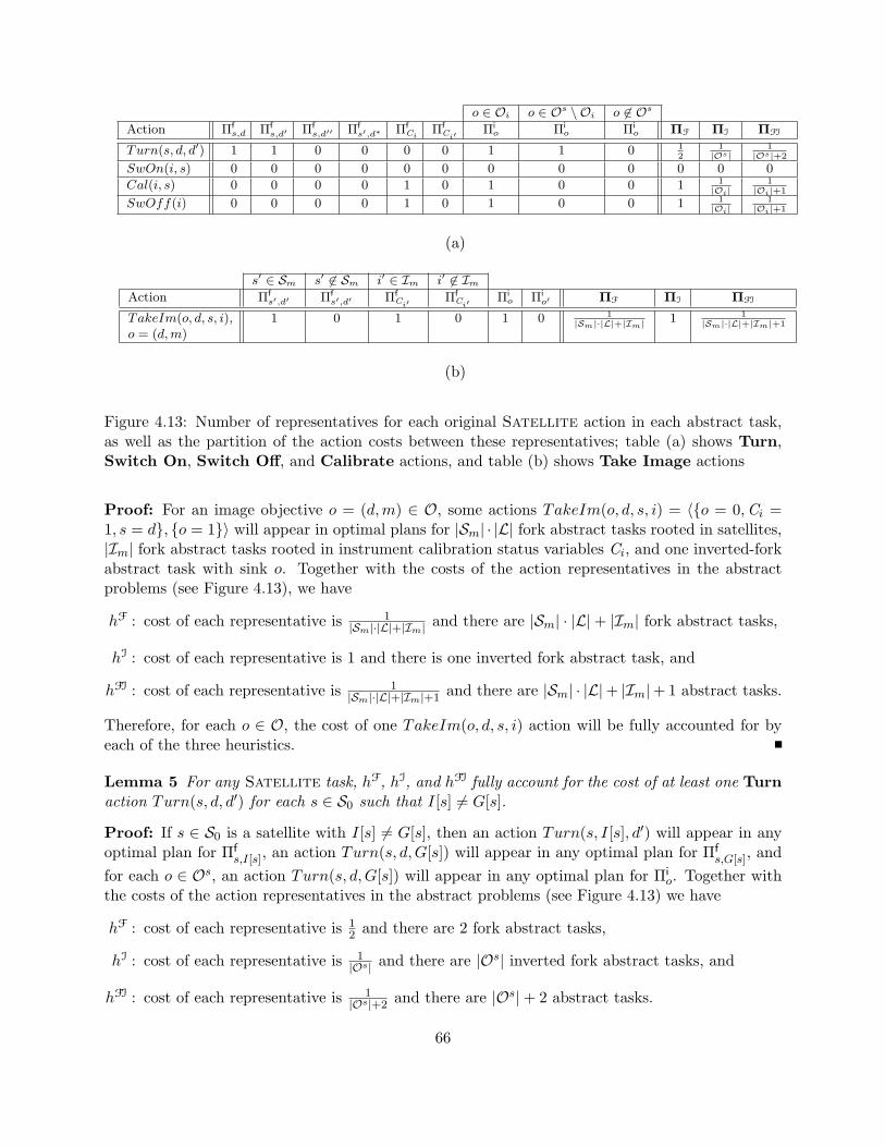
o ∈ Oi o ∈ Os \ Oi o 6∈ Os
Action Πfs,d Πf
s,d′ Πfs,d′′ Πf
s′,d∗ ΠfCi
ΠfCi′
Πio Πi
o Πio ΠF ΠI ΠFI
Turn(s, d, d′) 1 1 0 0 0 0 1 1 0 12
1|Os|
1|Os|+2
SwOn(i, s) 0 0 0 0 0 0 0 0 0 0 0 0
Cal(i, s) 0 0 0 0 1 0 1 0 0 1 1|Oi|
1|Oi|+1
SwOff(i) 0 0 0 0 1 0 1 0 0 1 1|Oi|
1|Oi|+1
(a)
s′ ∈ Sm s′ 6∈ Sm i′ ∈ Im i′ 6∈ ImAction Πf
s′,d′ Πfs′,d′ Πf
Ci′Πf
Ci′Πio Πi
o′ ΠF ΠI ΠFI
TakeIm(o, d, s, i),o = (d,m)
1 0 1 0 1 0 1|Sm|·|L|+|Im| 1 1
|Sm|·|L|+|Im|+1
(b)
Figure 4.13: Number of representatives for each original Satellite action in each abstract task,as well as the partition of the action costs between these representatives; table (a) shows Turn,Switch On, Switch Off, and Calibrate actions, and table (b) shows Take Image actions
Proof: For an image objective o = (d,m) ∈ O, some actions TakeIm(o, d, s, i) = 〈{o = 0,Ci =1, s = d}, {o = 1}〉 will appear in optimal plans for |Sm| · |L| fork abstract tasks rooted in satellites,|Im| fork abstract tasks rooted in instrument calibration status variables Ci, and one inverted-forkabstract task with sink o. Together with the costs of the action representatives in the abstractproblems (see Figure 4.13), we have
hF : cost of each representative is 1|Sm|·|L|+|Im| and there are |Sm| · |L|+ |Im| fork abstract tasks,
hI : cost of each representative is 1 and there is one inverted fork abstract task, and
hFI : cost of each representative is 1|Sm|·|L|+|Im|+1 and there are |Sm| · |L|+ |Im|+ 1 abstract tasks.
Therefore, for each o ∈ O, the cost of one TakeIm(o, d, s, i) action will be fully accounted for byeach of the three heuristics.
Lemma 5 For any Satellite task, hF, hI, and hFI fully account for the cost of at least one Turnaction Turn(s, d, d′) for each s ∈ S0 such that I[s] 6= G[s].
Proof: If s ∈ S0 is a satellite with I[s] 6= G[s], then an action Turn(s, I[s], d′) will appear in anyoptimal plan for Πf
s,I[s], an action Turn(s, d,G[s]) will appear in any optimal plan for Πfs,G[s], and
for each o ∈ Os, an action Turn(s, d,G[s]) will appear in any optimal plan for Πio. Together with
the costs of the action representatives in the abstract problems (see Figure 4.13) we have
hF : cost of each representative is 12 and there are 2 fork abstract tasks,
hI : cost of each representative is 1|Os| and there are |Os| inverted fork abstract tasks, and
hFI : cost of each representative is 1|Os|+2 and there are |Os|+ 2 abstract tasks.
66
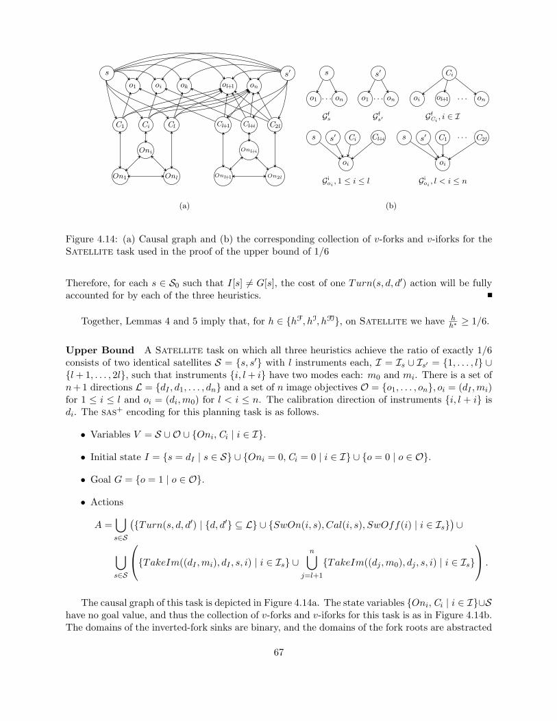
o1 oi ok ol+1 on
s s′
C1 ClCi Cl+1 C2lCl+i
On1 Onl
Oni
Onl+1 On2l
Onl+i
o1 . . . on
s
o1 . . . on
s′
oi ol+1 . . . on
Ci
oi
s s′ Ci Cl+i
oi
s s′ C1. . . C2l
(a) (b)
Gfs Gf
s′ GfCi, i ∈ I
G ioi, 1 ≤ i ≤ l G i
oi, l < i ≤ n
Figure 4.14: (a) Causal graph and (b) the corresponding collection of v-forks and v-iforks for theSatellite task used in the proof of the upper bound of 1/6
Therefore, for each s ∈ S0 such that I[s] 6= G[s], the cost of one Turn(s, d, d′) action will be fullyaccounted for by each of the three heuristics.
Together, Lemmas 4 and 5 imply that, for h ∈ {hF, hI, hFI}, on Satellite we have hh∗ ≥ 1/6.
Upper Bound A Satellite task on which all three heuristics achieve the ratio of exactly 1/6consists of two identical satellites S = {s, s′} with l instruments each, I = Is ∪ Is′ = {1, . . . , l} ∪{l+ 1, . . . , 2l}, such that instruments {i, l+ i} have two modes each: m0 and mi. There is a set ofn+ 1 directions L = {dI , d1, . . . , dn} and a set of n image objectives O = {o1, . . . , on}, oi = (dI ,mi)for 1 ≤ i ≤ l and oi = (di,m0) for l < i ≤ n. The calibration direction of instruments {i, l + i} isdi. The sas+ encoding for this planning task is as follows.
• Variables V = S ∪ O ∪ {Oni,Ci | i ∈ I}.
• Initial state I = {s = dI | s ∈ S} ∪ {Oni = 0,Ci = 0 | i ∈ I} ∪ {o = 0 | o ∈ O}.
• Goal G = {o = 1 | o ∈ O}.
• Actions
A =⋃s∈S
({Turn(s, d, d′) | {d, d′} ⊆ L} ∪ {SwOn(i, s), Cal(i, s), SwOff(i) | i ∈ Is}
)∪
⋃s∈S
{TakeIm((dI ,mi), dI , s, i) | i ∈ Is} ∪n⋃
j=l+1
{TakeIm((dj ,m0), dj , s, i) | i ∈ Is}
.
The causal graph of this task is depicted in Figure 4.14a. The state variables {Oni,Ci | i ∈ I}∪Shave no goal value, and thus the collection of v-forks and v-iforks for this task is as in Figure 4.14b.The domains of the inverted-fork sinks are binary, and the domains of the fork roots are abstracted
67
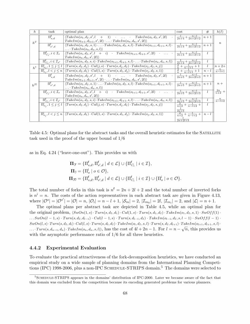
h task optimal plan cost # h(I)
hF
Πfs,d 〈TakeIm(o1, dI , s
′, l + 1) · . . . · TakeIm(ol, dI , s′, 2l) ·
TakeIm(ol+1, dl+1, s′, 2l) · . . . · TakeIm(on, dn, s′, 2l)〉
l2n+4
+ n−l2n+2l+2
n+ 1
nΠfs′,d 〈TakeIm(o1, dI , s, 1) · . . . ·TakeIm(ol, dI , s, l) ·TakeIm(ol+1, dl+1, s, l) ·
. . . · TakeIm(on, dn, s, l)〉l
2n+4+ n−l
2n+2l+2n+ 1
ΠfCi, i ∈ Is 〈TakeIm(oi, dI , s
′, l + i) · TakeIm(ol+1, dl+1, s′, 2l) · . . . ·
TakeIm(on, dn, s′, 2l)〉1
2n+4+ n−l
2n+2l+2l
ΠfCi, i ∈ Is′ 〈TakeIm(oi, dI , s, i) ·TakeIm(ol+1, dl+1, s, l) · . . . ·TakeIm(on, dn, s, l)〉 1
2n+4+ n−l
2n+2l+2l
hI Πioj, 1 ≤ j ≤ l 〈Turn(s, dI , dj) · Cal(j, s) · Turn(s, dj , dI) · TakeIm(oj , dI , s, j)〉 2
n+ 1n−l+1
+ 1 l n+ 2+n
n−l+1Πioj, l < j ≤ n 〈Turn(s, dI , d1) · Cal(1, s) · Turn(s, d1, dj) · TakeIm(oj , dI , s, 1)〉 2
n+ 1n−l+1
+ 1 n− l
hFI
Πfs,d 〈TakeIm(o1, dI , s
′, l + 1) · . . . · TakeIm(ol, dI , s′, 2l) ·
TakeIm(ol+1, dl+1, s′, 2l) · . . . · TakeIm(on, dn, s′, 2l)〉
l2n+5
+ n−l2n+2l+3
n+ 1
n +
2nn+2
+
nn−l+2
Πfs′,d 〈TakeIm(o1, dI , s, 1) · . . . ·TakeIm(ol, dI , s, l) ·TakeIm(ol+1, dl+1, s, l) ·
. . . · TakeIm(on, dn, s, l)〉l
2n+5+ n−l
2n+2l+3n+ 1
ΠfCi, i ∈ Is 〈TakeIm(oi, dI , s
′, l + i) · TakeIm(ol+1, dl+1, s′, 2l) · . . . ·
TakeIm(on, dn, s′, 2l)〉1
2n+5+ n−l
2n+2l+3l
ΠfCi, i ∈ Is′ 〈TakeIm(oi, dI , s, i) ·TakeIm(ol+1, dl+1, s, l) · . . . ·TakeIm(on, dn, s, l)〉 1
2n+5+ n−l
2n+2l+3l
Πioj, 1 ≤ j ≤ l 〈Turn(s, dI , dj) · Cal(j, s) · Turn(s, dj , dI) · TakeIm(oj , dI , s, j)〉 2
n+2+ 1n−l+2
+1
2n+5
l
Πioj, l < j ≤ n 〈Turn(s, dI , d1) · Cal(1, s) · Turn(s, d1, dj) · TakeIm(oj , dI , s, 1)〉 2
n+2+ 1n−l+2
+1
2n+2l+3
n− l
Table 4.5: Optimal plans for the abstract tasks and the overall heuristic estimates for the Satellitetask used in the proof of the upper bound of 1/6
as in Eq. 4.24 (“leave-one-out”). This provides us with
ΠF = {Πfs,d,Π
fs′,d | d ∈ L} ∪ {Πf
Ci | i ∈ I},ΠI = {Πi
o | o ∈ O},ΠFI = {Πf
s,d,Πfs′,d | d ∈ L} ∪ {Πf
Ci | i ∈ I} ∪ {Πio | o ∈ O}.
The total number of forks in this task is nf = 2n + 2l + 2 and the total number of inverted forksis ni = n. The costs of the action representatives in each abstract task are given in Figure 4.13,where |Os| = |Os′ | = |O| = n, |Oi| = n− l + 1, |Sm| = 2, |Im0 | = 2l, |Imi | = 2, and |L| = n+ 1.
The optimal plans per abstract task are depicted in Table 4.5, while an optimal plan forthe original problem, 〈SwOn(1, s) · Turn(s, dI , d1) · Cal(1, s) · Turn(s, d1, dI) · TakeIm(o1, dI , s, 1) · SwOff(1) ·. . . SwOn(l − 1, s) · Turn(s, dI , dl−1) · Cal(l − 1, s) · Turn(s, dl−1, dI) · TakeIm(ol−1, dI , s, l − 1) · SwOff(l − 1) ·SwOn(l, s) ·Turn(s, dI , dl) ·Cal(l, s) ·Turn(s, dl, dI) ·TakeIm(ol, dI , s, l) ·Turn(s, dI , dl+1) ·TakeIm(ol+1, dl+1, s, l) ·. . . · Turn(s, dn−1, dn) · TakeIm(on, dn, s, l)〉, has the cost of 4l+ 2n− 1. For l = n−√n, this provides uswith the asymptotic performance ratio of 1/6 for all three heuristics.
4.4.2 Experimental Evaluation
To evaluate the practical attractiveness of the fork-decomposition heuristics, we have conducted anempirical study on a wide sample of planning domains from the International Planning Competi-tions (IPC) 1998-2006, plus a non-IPC Schedule-STRIPS domain.5 The domains were selected to
5Schedule-STRIPS appears in the domains’ distribution of IPC-2000. Later we became aware of the fact thatthis domain was excluded from the competition because its encoding generated problems for various planners.
68
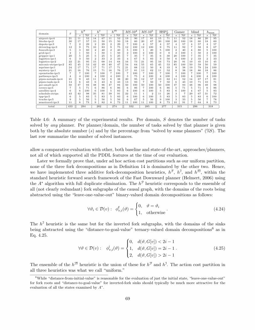
domain ShF hI hFI MS -104 MS -105 HSP∗F Gamer blind hmaxs %S s %S s %S s %S s %S s %S s %S s %S s %S
airport-ipc4 21 11 52 14 67 11 52 19 90 17 81 15 71 11 52 18 86 20 95blocks-ipc2 30 17 57 15 50 15 50 18 60 20 67 30 100 30 100 18 60 18 60depots-ipc3 7 2 29 2 29 2 29 7 100 4 57 4 57 4 57 4 57 4 57driverlog-ipc3 12 9 75 10 83 9 75 12 100 12 100 9 75 11 92 7 58 8 67freecell-ipc3 5 3 60 2 40 2 40 5 100 1 20 5 100 2 40 4 80 5 100grid-ipc1 2 1 50 1 50 1 50 2 100 2 100 0 0 2 100 1 50 2 100gripper-ipc1 20 5 25 5 25 5 25 7 35 7 35 6 30 20 100 7 35 7 35logistics-ipc1 6 3 50 2 33 2 33 4 67 5 83 3 50 6 100 2 33 2 33logistics-ipc2 22 21 95 15 68 14 64 16 73 21 95 16 73 20 91 10 45 10 45miconic-strips-ipc2 85 45 53 42 49 40 47 54 64 55 65 45 53 85 100 50 59 50 59mprime-ipc1 24 17 71 17 71 17 71 21 88 12 50 8 33 9 38 19 79 24 100mystery-ipc1 21 16 76 15 71 16 76 17 81 13 62 11 52 8 38 18 86 18 86openstacks-ipc5 7 7 100 7 100 7 100 7 100 7 100 7 100 7 100 7 100 7 100pathways-ipc5 4 4 100 4 100 4 100 3 75 4 100 4 100 4 100 4 100 4 100pipes-notank-ipc4 21 9 43 11 52 8 38 20 95 12 57 13 62 11 52 14 67 17 81pipes-tank-ipc4 14 6 43 6 43 6 43 13 93 7 50 7 50 6 43 10 71 10 71psr-small-ipc4 50 47 94 48 96 47 94 50 100 50 100 50 100 47 94 48 96 49 98rovers-ipc5 7 5 71 6 86 6 86 6 86 7 100 6 86 5 71 5 71 6 86satellite-ipc4 6 6 100 6 100 5 83 6 100 6 100 5 83 6 100 4 67 5 83schedule-strips 43 42 98 35 81 39 91 22 51 1 2 11 26 3 7 29 67 31 72tpp-ipc5 6 5 83 5 83 5 83 6 100 6 100 5 83 5 83 5 83 6 100trucks-ipc5 9 5 56 5 56 5 56 6 67 5 56 9 100 3 33 5 56 7 78zenotravel-ipc3 11 8 73 9 82 8 73 11 100 11 100 8 73 10 91 7 64 8 73
total 433 294 282 274 332 285 277 315 296 318
Table 4.6: A summary of the experimental results. Per domain, S denotes the number of taskssolved by any planner. Per planner/domain, the number of tasks solved by that planner is givenboth by the absolute number (s) and by the percentage from “solved by some planners” (%S). Thelast row summarize the number of solved instances.
allow a comparative evaluation with other, both baseline and state-of-the-art, approaches/planners,not all of which supported all the PDDL features at the time of our evaluation.
Later we formally prove that, under ad hoc action cost partitions such as our uniform partition,none of the three fork decompositions as in Definition 14 is dominated by the other two. Hence,we have implemented three additive fork-decomposition heuristics, hF, hI, and hFI, within thestandard heuristic forward search framework of the Fast Downward planner (Helmert, 2006) usingthe A∗ algorithm with full duplicate elimination. The hF heuristic corresponds to the ensemble ofall (not clearly redundant) fork subgraphs of the causal graph, with the domains of the roots beingabstracted using the “leave-one-value-out” binary-valued domain decompositions as follows:
∀ϑi ∈ D(v) : φfv,i(ϑ) =
{0, ϑ = ϑi
1, otherwise. (4.24)
The hI heuristic is the same but for the inverted fork subgraphs, with the domains of the sinksbeing abstracted using the “distance-to-goal-value” ternary-valued domain decompositions6 as inEq. 4.25.
∀ϑ ∈ D(v) : φiv,i(ϑ) =
0, d(ϑ,G[v]) < 2i− 11, d(ϑ,G[v]) = 2i− 12, d(ϑ,G[v]) > 2i− 1
. (4.25)
The ensemble of the hFI heuristic is the union of these for hF and hI. The action cost partition inall three heuristics was what we call “uniform.”
6While “distance-from-initial-value” is reasonable for the evaluation of just the initial state, “leave-one-value-out”for fork roots and “distance-to-goal-value” for inverted-fork sinks should typically be much more attractive for theevaluation of all the states examined by A∗.
69
We make a comparison with two baseline approaches, namely “blind A∗” with heuristic value0 for goal states and 1 otherwise, and A∗ with the hmax heuristic (Bonet & Geffner, 2001), as wellas with state-of-the-art abstraction heuristics, represented by the merge-and-shrink abstractionsof Helmert et al. (2007). The latter were constructed under the linear, f -preserving abstractionstrategy proposed by these authors, and this under two fixed bounds on the size of the abstractstate spaces, notably |Sα| < 104 and |Sα| < 105. These four (baseline and merge-and-shrink)heuristics were implemented by Helmert et al. (2007) within the same planning system as ourfork-decomposition heuristics, allowing for a fairly unbiased comparison. We also compare to theGamer (Edelkamp & Kissmann, 2009) and HSP∗F (Haslum, 2008) planners, the winner and therunner-up at the sequential optimization track of IPC-2008. On the algorithmic side, Gamer isbased on a bidirectional blind search using sophisticated symbolic-search techniques, and HSP∗Fuses A∗ with an additive critical-path heuristic. The experiments were conducted on a 3 GHzIntel E8400 CPU with 2 GB memory, using 1.5 GB memory limit and 30 minute timeout. Theonly exception was Gamer, for which we used similar machines but with 4 GB memory and 2 GBmemory limit; this was done to provide Gamer with the environment for which it was configured.
Table 4.6 summarizes our experimental results in terms of the number of tasks solved by eachplanner. Our impression of fork-decomposition heuristics from Table 4.6 is somewhat mixed. Onthe one hand, the performance of all three fork-decomposition based planners was comparable to oneof the settings of the merge-and-shrink heuristic, and this clearly testifies for that the framework ofimplicit abstractions is not of theoretical interest only. On the other hand, all the planners, exceptfor A∗ with the merge-and-shrink heuristic with |Sα| < 104, failed to outperform A∗ with thebaseline hmax heuristic. More important for us is that, unfortunately, all three fork-decompositionbased planners failed to outperform even the basic blind search.
This, however, is not the end of the story for the fork-decomposition heuristics. Some hope canbe found in the detailed results in Tables B.1-B.6 (pp. 177-182). As it appears from Table B.2, on,e.g., the Logistics-ipc2 domain, hF almost consistently leads to expanding fewer search nodesthan the (better between the two merge-and-shrink heuristics on this domain) MS -105, with thedifference hitting four orders of magnitude. However, the time complexity of hF per search nodeis substantially higher than that of MS -105, with the two expanding at a rate of approximately40 and 100000 nodes per second, respectively. The outcome is simple: while with no time limits(and only memory limit of 1.5 GB) hF solves more tasks in Logistics-ipc2 than MS -105 (task12-1 is solved with hF in 2519.01 seconds), this is not so with a standard time limit of half an hourused for Table B.2. In what follows we examine the possibility of exploiting the informativeness offork-decomposition heuristics while not falling into the trap of costly per-node heuristic evaluation.
4.5 Back to Theory: h-Partitions and Databased Implicit Abstrac-tions
Accuracy and low time complexity are both desired yet competing properties of heuristic functions.For many powerful heuristics, and abstraction heuristics in particular, computing h(s) for each states in isolation is impractical: while computing h(s) is polynomial in the description size of Π, it isoften not efficient enough to be performed at each search node. However, for some costly heuristicsthis obstacle can be largely overcome by sharing most of the computation between the evaluationsof h on different states. If that is possible, the shared parts of computing h for all problem states areprecomputed and memorized before the search, and then reused during the search by the evaluations
70
of h on different states. Such a mixed offline/online heuristic computation is henceforth called h-partition, and we define the time complexity of an h-partition as the complexity of computing hfor a set of states. Given a subset of k problem states S′ ⊆ S, the h-partition’s time complexity ofcomputing {h(s) | s ∈ S′} is expressed as O(X + kY ), where O(X) and O(Y ) are, respectively, thecomplexity of the (offline) pre-search and (online) per-node parts of computing h(s).
These days h-partitions are being adopted by various optimal planners using critical-path heuris-tics hm for m > 1 (Haslum et al., 2005), landmark heuristics hL and hLA (Karpas & Domshlak,2009), and PDB and merge-and-shrink abstraction heuristics (Edelkamp, 2001; Helmert et al.,2007). Without effective h-partitions, optimal search with these heuristics would not scale up well,while with such h-partitions it constitutes the state of the art of cost-optimal planning. For instance,a very attractive property of PDB abstractions is the complexity of their natural hα-partition. In-stead of computing hα(s) = h∗(α(s)) from scratch for each evaluated state s (impractical for allbut tiny projections), the practice is to precompute and store h∗(s′) for all abstract states s′ ∈ Sα,after which the per-node computation of hα(s) boils down to a hash-table lookup for h∗(α(s)) witha perfect hash function. In our terms, the time and space complexity of that PDB hα-partition fora set of k states is O(|Sα|(log(|Sα|) + |A|) + k) and O(|Sα|), respectively. This is precisely whatmakes PDB heuristics so attractive in practice. In that respect, the picture with merge-and-shrinkabstractions is very much similar. While the order in which composites are formed and the choiceof abstract states to contract are crucial to the complexity of their natural hα-partitions, the timeand space complexity for the concrete linear abstraction strategy of Helmert et al. are respectivelyO(|V ||Sα|(log(|Sα|) + |A|) + k · |V |) and O(|Sα|). Similarly to PDB abstractions, the per-nodecomputation of hα(s) with a merge-and-shrink abstraction α is just a lookup in a data structurestoring h∗(α(s)) for all abstract states α(s) ∈ Sα. Hence, while the pre-search computation withMS abstractions can be more costly than with PDBs, the online part of computing heuristic valuesis still extremely efficient. This per-node efficiency provides the merge-and-shrink heuristics withimpressive practical effectiveness on numerous IPC domains (Helmert et al., 2007).
To sum up, we can say that the fixed size of abstract spaces induced by explicit abstractionssuch as PDBs and merge-and-shrink is not only a limitation but also a key to obtaining effective h-partitions. In contrast, escaping that limitation with implicit abstractions might trap us into havingto pay a high price for each search-node evaluation. We now show, however, that the time-per-nodecomplexity bottleneck of fork-decomposition heuristics can be successfully overcome. Specifically,we show that an equivalent of PDB’s and merge-and-shrink notion of “database” exists for fork-decomposition abstractions as well, despite their exponential-size abstract spaces. Of course, unlikewith PDB and merge-and-shrink abstractions, the databased fork-decomposition heuristics do not(and cannot) provide us with a purely lookup online computation of hα(s). The online part of thehα-partition has to be nontrivial in the sense that its complexity cannot be O(1). In what comesnext we prove the existence of such effective h-partitions for fork and inverted fork abstractions. InSection 4.5.3 we then empirically show that these h-partitions lead to fast pre-search and per-nodecomputations, allowing the informativeness of the fork-decomposition heuristics to be successfullyexploited in practice.
4.5.1 Fork Databases
Theorem 11 Let Π = 〈V,A, I,G, cost〉 be a planning task with a fork causal graph rooted at abinary-valued variable r. There exists an h∗-partition for Π such that, for any set of k states, thetime and space complexity of that h∗-partition is, respectively, O(d3|V |+|Ar|+kd|V |) and O(d2|V |),
71
where d = maxv D(v).
Proof: The proof is by a modification of the polynomial-time algorithm for computing h∗(s) fora state s of such a task Π used in the proof of Theorem 4 (Tractable Forks). Given a state s, letD(r) = {0, 1}, where s[r] = 0. In what follows, for each of the two root’s values ϑ ∈ D(r), ¬ϑdenotes the opposite value 1 − ϑ; σ(r), �∗[σ(r)], DTG0
v and DTG1v are defined exactly as in the
proof of Theorem 4.
(1) For each of the two values ϑr ∈ D(r) of the root variable, each leaf variable v ∈ V \ {r}, andeach pair of values ϑ, ϑ′ ∈ D(v), let pϑ,ϑ′;ϑr be the cost of the cheapest sequence of actionschanging v from ϑ to ϑ′ provided r = ϑr. The whole set {pϑ,ϑ′;ϑr} for all the leaves v ∈ V \ {r}can be computed by a straightforward variant of the all-pairs-shortest-paths, Floyd-Warshallalgorithm on DTGϑr
v in time O(d3|V |).
(2) For each leaf variable v ∈ V \ {r}, 1 ≤ i ≤ d + 1, and ϑ ∈ D(v), let gϑ;i be the cost of thecheapest sequence of actions changing s[v] to ϑ provided a sequence σ ∈ �∗[σ(r)], |σ| = i, ofvalue changes of r. Having the values {pϑ,ϑ′;ϑr} from step (1), the set {gϑ;i} is given by thesolution of the recursive equation
gϑ;i =
ps[v],ϑ;s[r], i = 1
minϑ′
[gϑ′;i−1 + pϑ′,ϑ;s[r]
], 1 < i ≤ δϑ, i is odd
minϑ′
[gϑ′;i−1 + pϑ′,ϑ;¬s[r]
], 1 < i ≤ δϑ, i is even
gϑ;i−1, δϑ < i ≤ d+ 1
,
where δϑ = |D(v)|+ 1. Given that, we have
h∗(s) = minσ∈�∗[σ(r)]
cost(σ) +∑
v∈V \{r}
gG[v];|σ|
,with cost(σ) =
∑|σ|i=2 cost(aσ[i]), where aσ[i] ∈ A is the cheapest action changing the value of r
from σ[i− 1] to σ[i].
Note that step (1) is already state-independent, but the heavy step (2) is not. However, thestate dependence of step (2) can mostly be overcome as follows. For each v ∈ V \ {r}, ϑ ∈ D(v),1 ≤ i ≤ d+ 1, and ϑr ∈ D(r), let gϑ;i(ϑr) be the cost of the cheapest sequence of actions changingϑ to G[v] provided the value changes of r induce a 0/1 sequence of length i starting with ϑr. Theset {gϑ;i(ϑr)} is given by the solution of the recursive equation
gϑ;i(ϑr) =
pϑ,G[v];ϑr , i = 1minϑ′
[gϑ′;i−1(¬ϑr) + pϑ,ϑ′;ϑr
], 1 < i ≤ δϑ
gϑ;i−1(ϑr), δϑ < i ≤ d+ 1
, (4.26)
which can be solved in time O(d3|V |). Note that this equation is now independent of the evaluatedstate s, and yet {gϑ;i(ϑr)} allow for computing h∗(s) for a given state s via
h∗(s) = minσ∈�∗[σ(r|s[r])]
cost(σ) +∑
v∈V \{r}
gs[v];|σ|(s[r])
(4.27)
72
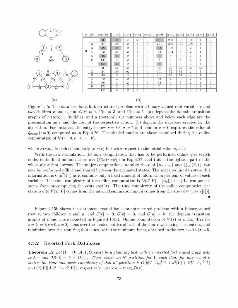
0 1
24
24
0
1 2
3
0
1
2
3
4
5
11
0100
01
11
01
11
01
11
01
150
150
0100
0100
r |σ| cost(σ) v=0 v=1 v=2 v=3 u=0 u=1 u=2 u=3 u=4 u=5
0
1 0 100 ∞ ∞ 0 201 200 101 100 1 02 24 100 2 1 0 201 200 101 100 1 0
3 48 100 2 1 0 53 102 3 2 1 04 72 100 2 1 0 53 102 3 2 1 0
5 96 3 2 1 0 5 4 3 2 1 06 120 3 2 1 0 5 4 3 2 1 0
7 144 3 2 1 0 5 4 3 2 1 0
1
1 0 ∞ ∞ 1 0 ∞ ∞ ∞ ∞ ∞ 02 24 100 ∞ 1 0 101 52 51 2 1 03 48 3 2 1 0 101 52 51 2 1 04 72 3 2 1 0 53 4 3 2 1 05 96 3 2 1 0 53 4 3 2 1 06 120 3 2 1 0 5 4 3 2 1 07 144 3 2 1 0 5 4 3 2 1 0
(a) (b)
Figure 4.15: The database for a fork-structured problem with a binary-valued root variable r andtwo children v and u, and G[r] = 0, G[v] = 3, and G[u] = 5. (a) depicts the domain transitiongraphs of r (top), v (middle), and u (bottom); the numbers above and below each edge are theprecondition on r and the cost of the respective action. (b) depicts the database created by thealgorithm. For instance, the entry in row r= 0 ∧ |σ|= 5 and column v = 0 captures the value ofgv=0;5(r=0) computed as in Eq. 4.26. The shaded entries are those examined during the onlinecomputation of h∗(r=0, v=0, u=0).
where σ(r|ϑr) is defined similarly to σ(r) but with respect to the initial value ϑr of r.With the new formulation, the only computation that has to be performed online, per search
node, is the final minimization over �∗[σ(r|s[r])] in Eq. 4.27, and this is the lightest part of thewhole algorithm anyway. The major computations, notably those of {pϑ,ϑ′;ϑr} and {gϑ;i(ϑr)}, cannow be performed offline and shared between the evaluated states. The space required to store thisinformation is O(d2|V |) as it contains only a fixed amount of information per pair of values of eachvariable. The time complexity of the offline computation is O(d3|V | + |Ar|); the |Ar| componentstems from precomputing the costs cost(σ). The time complexity of the online computation perstate is O(d|V |); |V | comes from the internal summation and d comes from the size of �∗[σ(r|s[r])].
Figure 4.15b shows the database created for a fork-structured problem with a binary-valuedroot r, two children v and u, and G[r] = 0, G[v] = 3, and G[u] = 5; the domain transitiongraphs of v and u are depicted in Figure 4.15(a). Online computation of h∗(s) as in Eq. 4.27 fors = (r=0, v=0, u=0) sums over the shaded entries of each of the four rows having such entries, andminimizes over the resulting four sums, with the minimum being obtained in the row r=0∧|σ|=5.
4.5.2 Inverted Fork Databases
Theorem 12 Let Π = 〈V ,A, I ,G, cost〉 be a planning task with an inverted fork causal graph withsink r and |D(r)| = b = O(1). There exists an h∗-partition for Π such that, for any set of kstates, the time and space complexity of that h∗-partition is O(b|V ||Ar|b−1 + d3|V | + k|V ||Ar|b−1)and O(|V ||Ar|b−1 + d2|V |), respectively, where d = maxv D(v).
73
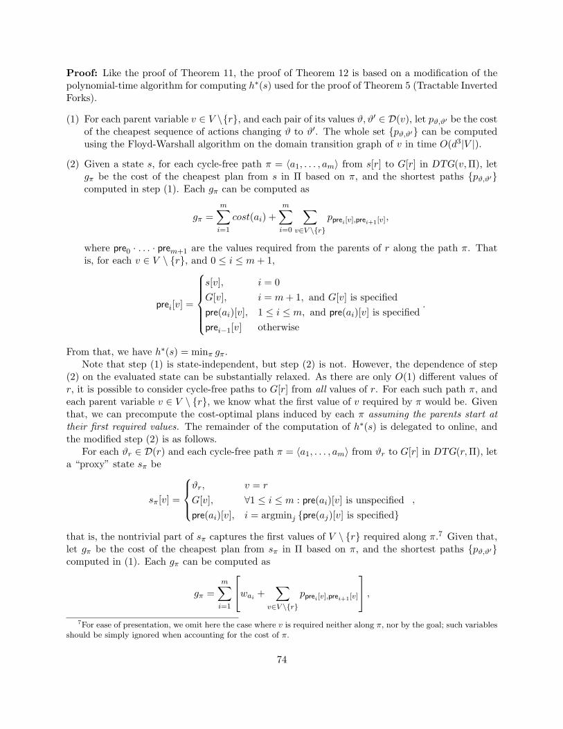
Proof: Like the proof of Theorem 11, the proof of Theorem 12 is based on a modification of thepolynomial-time algorithm for computing h∗(s) used for the proof of Theorem 5 (Tractable InvertedForks).
(1) For each parent variable v ∈ V \{r}, and each pair of its values ϑ, ϑ′ ∈ D(v), let pϑ,ϑ′ be the costof the cheapest sequence of actions changing ϑ to ϑ′. The whole set {pϑ,ϑ′} can be computedusing the Floyd-Warshall algorithm on the domain transition graph of v in time O(d3|V |).
(2) Given a state s, for each cycle-free path π = 〈a1, . . . , am〉 from s[r] to G[r] in DTG(v,Π), letgπ be the cost of the cheapest plan from s in Π based on π, and the shortest paths {pϑ,ϑ′}computed in step (1). Each gπ can be computed as
gπ =m∑i=1
cost(ai) +m∑i=0
∑v∈V \{r}
pprei[v],prei+1[v],
where pre0 · . . . · prem+1 are the values required from the parents of r along the path π. Thatis, for each v ∈ V \ {r}, and 0 ≤ i ≤ m+ 1,
prei[v] =
s[v], i = 0G[v], i = m+ 1, and G[v] is specifiedpre(ai)[v], 1 ≤ i ≤ m, and pre(ai)[v] is specifiedprei−1[v] otherwise
.
From that, we have h∗(s) = minπ gπ.Note that step (1) is state-independent, but step (2) is not. However, the dependence of step
(2) on the evaluated state can be substantially relaxed. As there are only O(1) different values ofr, it is possible to consider cycle-free paths to G[r] from all values of r. For each such path π, andeach parent variable v ∈ V \ {r}, we know what the first value of v required by π would be. Giventhat, we can precompute the cost-optimal plans induced by each π assuming the parents start attheir first required values. The remainder of the computation of h∗(s) is delegated to online, andthe modified step (2) is as follows.
For each ϑr ∈ D(r) and each cycle-free path π = 〈a1, . . . , am〉 from ϑr to G[r] in DTG(r,Π), leta “proxy” state sπ be
sπ[v] =
ϑr, v = r
G[v], ∀1 ≤ i ≤ m : pre(ai)[v] is unspecifiedpre(ai)[v], i = argminj {pre(aj)[v] is specified}
,
that is, the nontrivial part of sπ captures the first values of V \ {r} required along π.7 Given that,let gπ be the cost of the cheapest plan from sπ in Π based on π, and the shortest paths {pϑ,ϑ′}computed in (1). Each gπ can be computed as
gπ =m∑i=1
wai +∑
v∈V \{r}
pprei[v],prei+1[v]
,7For ease of presentation, we omit here the case where v is required neither along π, nor by the goal; such variables
should be simply ignored when accounting for the cost of π.
74
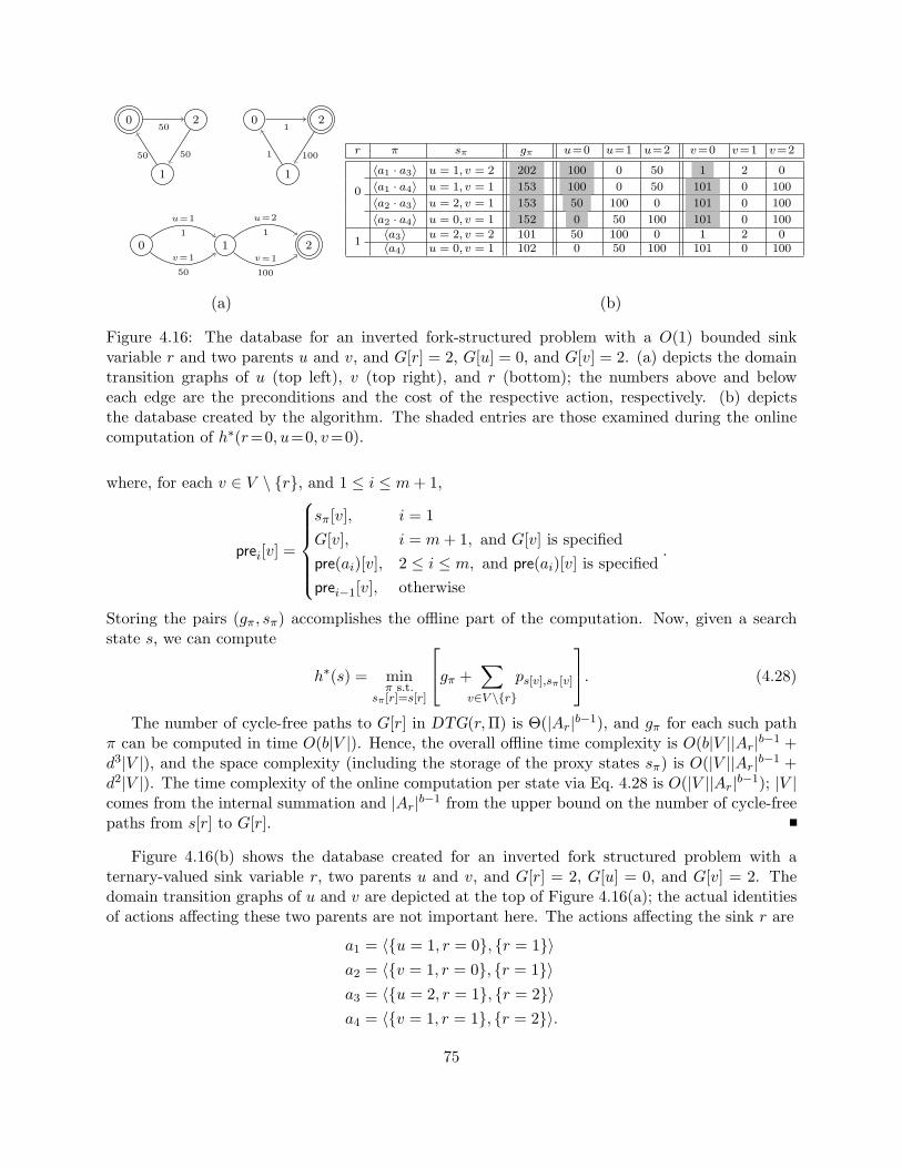
0
1
2 0
1
2
0 1 2
50
5050
1
1001
50
v=1
1
u=1
100
v=1
1
u=2
r π sπ gπ u=0 u=1 u=2 v=0 v=1 v=2
0
〈a1 · a3〉 u = 1, v = 2 202 100 0 50 1 2 0
〈a1 · a4〉 u = 1, v = 1 153 100 0 50 101 0 100
〈a2 · a3〉 u = 2, v = 1 153 50 100 0 101 0 100
〈a2 · a4〉 u = 0, v = 1 152 0 50 100 101 0 100
1〈a3〉 u = 2, v = 2 101 50 100 0 1 2 0〈a4〉 u = 0, v = 1 102 0 50 100 101 0 100
(a) (b)
Figure 4.16: The database for an inverted fork-structured problem with a O(1) bounded sinkvariable r and two parents u and v, and G[r] = 2, G[u] = 0, and G[v] = 2. (a) depicts the domaintransition graphs of u (top left), v (top right), and r (bottom); the numbers above and beloweach edge are the preconditions and the cost of the respective action, respectively. (b) depictsthe database created by the algorithm. The shaded entries are those examined during the onlinecomputation of h∗(r=0, u=0, v=0).
where, for each v ∈ V \ {r}, and 1 ≤ i ≤ m+ 1,
prei[v] =
sπ[v], i = 1G[v], i = m+ 1, and G[v] is specifiedpre(ai)[v], 2 ≤ i ≤ m, and pre(ai)[v] is specifiedprei−1[v], otherwise
.
Storing the pairs (gπ, sπ) accomplishes the offline part of the computation. Now, given a searchstate s, we can compute
h∗(s) = minπ s.t.
sπ [r]=s[r]
gπ +∑
v∈V \{r}
ps[v],sπ [v]
. (4.28)
The number of cycle-free paths to G[r] in DTG(r,Π) is Θ(|Ar|b−1), and gπ for each such pathπ can be computed in time O(b|V |). Hence, the overall offline time complexity is O(b|V ||Ar|b−1 +d3|V |), and the space complexity (including the storage of the proxy states sπ) is O(|V ||Ar|b−1 +d2|V |). The time complexity of the online computation per state via Eq. 4.28 is O(|V ||Ar|b−1); |V |comes from the internal summation and |Ar|b−1 from the upper bound on the number of cycle-freepaths from s[r] to G[r].
Figure 4.16(b) shows the database created for an inverted fork structured problem with aternary-valued sink variable r, two parents u and v, and G[r] = 2, G[u] = 0, and G[v] = 2. Thedomain transition graphs of u and v are depicted at the top of Figure 4.16(a); the actual identitiesof actions affecting these two parents are not important here. The actions affecting the sink r are
a1 = 〈{u = 1, r = 0}, {r = 1}〉a2 = 〈{v = 1, r = 0}, {r = 1}〉a3 = 〈{u = 2, r = 1}, {r = 2}〉a4 = 〈{v = 1, r = 1}, {r = 2}〉.
75
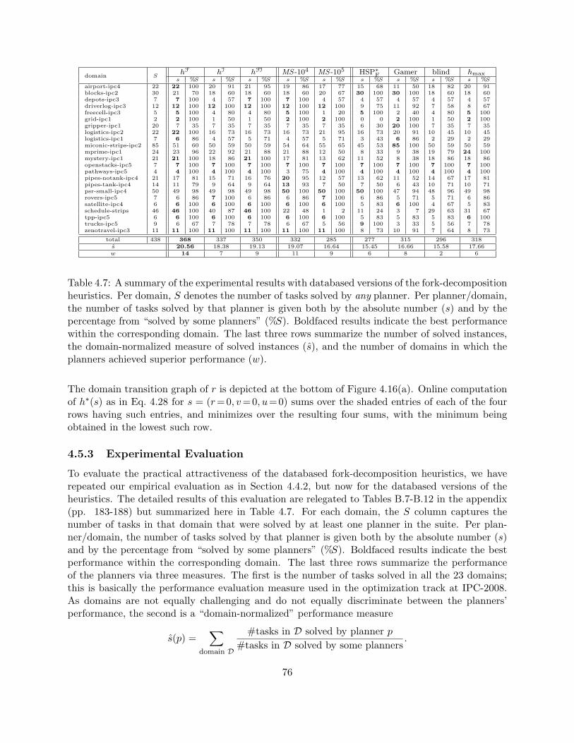
domain ShF hI hFI MS -104 MS -105 HSP∗F Gamer blind hmaxs %S s %S s %S s %S s %S s %S s %S s %S s %S
airport-ipc4 22 22 100 20 91 21 95 19 86 17 77 15 68 11 50 18 82 20 91blocks-ipc2 30 21 70 18 60 18 60 18 60 20 67 30 100 30 100 18 60 18 60depots-ipc3 7 7 100 4 57 7 100 7 100 4 57 4 57 4 57 4 57 4 57driverlog-ipc3 12 12 100 12 100 12 100 12 100 12 100 9 75 11 92 7 58 8 67freecell-ipc3 5 5 100 4 80 4 80 5 100 1 20 5 100 2 40 4 80 5 100grid-ipc1 2 2 100 1 50 1 50 2 100 2 100 0 0 2 100 1 50 2 100gripper-ipc1 20 7 35 7 35 7 35 7 35 7 35 6 30 20 100 7 35 7 35logistics-ipc2 22 22 100 16 73 16 73 16 73 21 95 16 73 20 91 10 45 10 45logistics-ipc1 7 6 86 4 57 5 71 4 57 5 71 3 43 6 86 2 29 2 29miconic-strips-ipc2 85 51 60 50 59 50 59 54 64 55 65 45 53 85 100 50 59 50 59mprime-ipc1 24 23 96 22 92 21 88 21 88 12 50 8 33 9 38 19 79 24 100mystery-ipc1 21 21 100 18 86 21 100 17 81 13 62 11 52 8 38 18 86 18 86openstacks-ipc5 7 7 100 7 100 7 100 7 100 7 100 7 100 7 100 7 100 7 100pathways-ipc5 4 4 100 4 100 4 100 3 75 4 100 4 100 4 100 4 100 4 100pipes-notank-ipc4 21 17 81 15 71 16 76 20 95 12 57 13 62 11 52 14 67 17 81pipes-tank-ipc4 14 11 79 9 64 9 64 13 93 7 50 7 50 6 43 10 71 10 71psr-small-ipc4 50 49 98 49 98 49 98 50 100 50 100 50 100 47 94 48 96 49 98rovers-ipc5 7 6 86 7 100 6 86 6 86 7 100 6 86 5 71 5 71 6 86satellite-ipc4 6 6 100 6 100 6 100 6 100 6 100 5 83 6 100 4 67 5 83schedule-strips 46 46 100 40 87 46 100 22 48 1 2 11 24 3 7 29 63 31 67tpp-ipc5 6 6 100 6 100 6 100 6 100 6 100 5 83 5 83 5 83 6 100trucks-ipc5 9 6 67 7 78 7 78 6 67 5 56 9 100 3 33 5 56 7 78zenotravel-ipc3 11 11 100 11 100 11 100 11 100 11 100 8 73 10 91 7 64 8 73
total 438 368 337 350 332 285 277 315 296 318s 20.56 18.38 19.13 19.07 16.64 15.45 16.66 15.58 17.66w 14 7 9 11 9 6 8 2 6
Table 4.7: A summary of the experimental results with databased versions of the fork-decompositionheuristics. Per domain, S denotes the number of tasks solved by any planner. Per planner/domain,the number of tasks solved by that planner is given both by the absolute number (s) and by thepercentage from “solved by some planners” (%S). Boldfaced results indicate the best performancewithin the corresponding domain. The last three rows summarize the number of solved instances,the domain-normalized measure of solved instances (s), and the number of domains in which theplanners achieved superior performance (w).
The domain transition graph of r is depicted at the bottom of Figure 4.16(a). Online computationof h∗(s) as in Eq. 4.28 for s = (r= 0, v= 0, u= 0) sums over the shaded entries of each of the fourrows having such entries, and minimizes over the resulting four sums, with the minimum beingobtained in the lowest such row.
4.5.3 Experimental Evaluation
To evaluate the practical attractiveness of the databased fork-decomposition heuristics, we haverepeated our empirical evaluation as in Section 4.4.2, but now for the databased versions of theheuristics. The detailed results of this evaluation are relegated to Tables B.7-B.12 in the appendix(pp. 183-188) but summarized here in Table 4.7. For each domain, the S column captures thenumber of tasks in that domain that were solved by at least one planner in the suite. Per plan-ner/domain, the number of tasks solved by that planner is given both by the absolute number (s)and by the percentage from “solved by some planners” (%S). Boldfaced results indicate the bestperformance within the corresponding domain. The last three rows summarize the performanceof the planners via three measures. The first is the number of tasks solved in all the 23 domains;this is basically the performance evaluation measure used in the optimization track at IPC-2008.As domains are not equally challenging and do not equally discriminate between the planners’performance, the second is a “domain-normalized” performance measure
s(p) =∑
domain D
#tasks in D solved by planner p#tasks in D solved by some planners
.
76
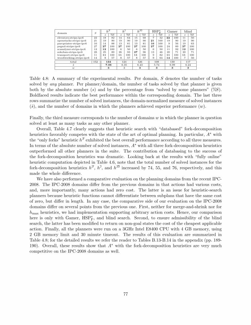
domain ShF hI hFI HSP∗F Gamer blinds %S s %S s %S s %S s %S s %S
elevators-strips-ipc6 22 18 82 14 64 15 68 7 32 22 100 11 50openstacks-strips-ipc6 21 19 90 19 90 19 90 21 100 19 90 19 90parcprinter-strips-ipc6 16 14 88 13 81 13 81 16 100 9 56 10 63pegsol-strips-ipc6 27 27 100 27 100 27 100 27 100 24 89 27 100scanalyzer-strips-ipc6 12 12 100 6 50 6 50 6 50 11 92 12 100sokoban-strips-ipc6 28 25 89 26 93 27 96 13 46 20 71 20 71transport-strips-ipc6 11 11 100 11 100 11 100 9 82 11 100 11 100woodworking-strips-ipc6 14 8 57 8 57 8 57 9 64 14 100 7 50
total 152 134 124 126 108 130 117s 7.06 6.35 6.43 5.74 6.99 6.24w 3 2 3 3 3 3
Table 4.8: A summary of the experimental results. Per domain, S denotes the number of taskssolved by any planner. Per planner/domain, the number of tasks solved by that planner is givenboth by the absolute number (s) and by the percentage from “solved by some planners” (%S).Boldfaced results indicate the best performance within the corresponding domain. The last threerows summarize the number of solved instances, the domain-normalized measure of solved instances(s), and the number of domains in which the planners achieved superior performance (w).
Finally, the third measure corresponds to the number of domains w in which the planner in questionsolved at least as many tasks as any other planner.
Overall, Table 4.7 clearly suggests that heuristic search with “databased” fork-decompositionheuristics favorably competes with the state of the art of optimal planning. In particular, A∗ withthe “only forks” heuristic hF exhibited the best overall performance according to all three measures.In terms of the absolute number of solved instances, A∗ with all three fork-decomposition heuristicsoutperformed all other planners in the suite. The contribution of databasing to the success ofthe fork-decomposition heuristics was dramatic. Looking back at the results with “fully online”heuristic computation depicted in Table 4.6, note that the total number of solved instances for thefork-decomposition heuristics hF, hI, and hFI increased by 74, 55, and 76, respectively, and thismade the whole difference.
We have also performed a comparative evaluation on the planning domains from the recent IPC-2008. The IPC-2008 domains differ from the previous domains in that actions had various costs,and, more importantly, many actions had zero cost. The latter is an issue for heuristic-searchplanners because heuristic functions cannot differentiate between subplans that have the same costof zero, but differ in length. In any case, the comparative side of our evaluation on the IPC-2008domains differ on several points from the previous one. First, neither for merge-and-shrink nor forhmax heuristics, we had implementation supporting arbitrary action costs. Hence, our comparisonhere is only with Gamer, HSP∗F, and blind search. Second, to ensure admissibility of the blindsearch, the latter has been modified to return on non-goal states the cost of the cheapest applicableaction. Finally, all the planners were run on a 3GHz Intel E8400 CPU with 4 GB memory, using2 GB memory limit and 30 minute timeout. The results of this evaluation are summarized inTable 4.8; for the detailed results we refer the reader to Tables B.13-B.14 in the appendix (pp. 189-190). Overall, these results show that A∗ with the fork-decomposition heuristics are very muchcompetitive on the IPC-2008 domains as well.
77

78
Chapter 5
Abstraction-based HeuristicsComposition
Since the late 1990s, numerous admissible heuristics for domain-independent planning have beenproposed and found practically effective, with research in this direction continuously expanding.Of course, as planning is known to be NP-hard even for extremely conservative planning for-malisms (Bylander, 1994), no heuristic should be expected to work well in all planning tasks.Moreover, even for a fixed planning task, no tractable heuristic will home in on all the “combina-torics” of the task at hand. The promise, however, is that different heuristics will target differentsources of the planning complexity, and composing a set of heuristics to exploit their individualstrengths could allow a larger range of planning tasks to be solved and each individual task to besolved more efficiently.
In this chapter we focus on the fundamental question of how one should better compose aset of admissible heuristics in solving a given planning task. One of the well-known and heavily-used properties of admissible heuristics is that taking the maximum of their values maximizesinformativeness while preserving admissibility. A more recent, alternative approach to composing aset of admissible heuristics corresponds to carefully separating the information used by the differentheuristics in the set so that their values could be summed instead of maximized over. This directionwas first exploited in the works on additive pattern database (PDB) heuristics (Edelkamp, 2001;Felner et al., 2004; Haslum et al., 2007), and more recently, in the scope of constrained PDBs, m-reachability, and implicit abstraction (also known as structural-pattern) heuristics (Haslum et al.,2005; Katz & Domshlak, 2008c).
The basic idea underlying all these additive heuristic ensembles is elegantly simple: for eachplanning task’s action a, if it can possibly be counted by more than one heuristic in the ensemble,then one should ensure that the cumulative counting of the cost of a does not exceed its true costin the original task. Such action cost partitioning was originally achieved by accounting for thewhole cost of each action in computing a single heuristic in the ensemble, while ignoring the costof that action in computing all the other heuristics in the ensemble (Edelkamp, 2001; Felner et al.,2004; Haslum et al., 2005). Recently, this “all-in-one/nothing-in-rest” action-cost partitioning hasbeen generalized by Katz and Domshlak (2007a, 2008c) and Yang et al. (2007, 2008) to arbitrarypartitioning of the action cost among the heuristics in the ensemble.
The great flexibility of additive heuristic ensembles, however, is a mixed blessing. For better orfor worse, the methodology of taking the maximum over the values provided by an arbitrary set of
79
independently constructed admissible heuristics is entirely nonparametric. By contrast, switching toadditive heuristic ensembles requires selecting an action-cost partitioning scheme, and this decisionproblem poses a number of computational challenges:
• The space of alternative action-cost partitions is infinite as the cost of each action can bepartitioned into an arbitrary set of nonnegative real numbers, the sum of which does notexceed the cost of that action.
• At least in domain-independent planning, our goal is a fully unsupervised decision process.
• Last but not least, the relative quality of each action-cost partition (in terms of the accuracyof the resulting additive heuristic) may vary dramatically between the examined search states.Hence, the choice of the action-cost partitioning scheme should ultimately be a function ofthe search state in question.
These concerns may explain why all previous works on both domain-specific and domain-independent additive heuristic ensembles adopt this or another ad hoc, fixed choice of action-costpartition. Consequently, all the reported empirical comparative evaluations of various max-basedand additive heuristic ensembles are inconclusive—for some search states along the search pro-cess, the (pre-selected) additive heuristic was found to dominate the max-combination, while forthe other states the opposite was the case. In the context of domain-specific additive PDBs, Yanget al. (2007) conclude that “determining which abstractions [here: action-cost partitioning schemes]will produce additives that are better than max over standards is still a big research issue.”
Focusing on abstraction heuristics, our contribution in this chapter is precisely in addressingthe problem of choosing the right action-cost partitioning over a given set of heuristics:
1. We provide a procedure that, given (i) a classical planning task Π, (ii) a forward-search states of Π, and (iii) a set of heuristics based on abstractions of Π, derives an optimal action-costpartition for s, that is, a partition that maximizes the heuristic estimate of that state. Theprocedure is fully unsupervised, and is based on a linear programming formulation of thatoptimization problem.
2. We show that the time complexity of our procedure is polynomial for arbitrary sets of allabstraction-based heuristic functions with which we are familiar. Such “procedure-friendly”heuristics include PDBs (Edelkamp, 2001; Yang et al., 2007), constrained PDBs (Haslumet al., 2005), merge-and-shrink abstractions (Helmert et al., 2007), fork-decomposition im-plicit abstractions (Katz & Domshlak, 2008c), and implicit abstractions based on tractableconstraint optimization over tree-shaped constraint networks (Katz & Domshlak, 2008a).Note that the estimate provided by a max-based ensemble corresponds to the estimate pro-vided by the respective additive ensemble under some action-cost partitioning. Thus, byfinding an optimal action-cost partition we provide a formally complete answer to the afore-mentioned question of “to add or not to add” in the context of abstraction heuristics.
Taking the fork-decomposition abstractions as a case study, we evaluate the empirical effective-ness of switching from ad hoc to optimal additive composition. Our evaluation on a wide rangeof International Planning Competition (IPC) benchmarks shows a substantial reduction in thenumber of nodes expanded by the A∗ algorithm. However, in the standard time-bounded setting,this reduction in expanded nodes is typically negatively balanced by the much more expensive
80
per-node computation of the optimal additive heuristic. To overcome this pitfall without forfeitingthe promise of optimized action cost partitions altogether, we suggest that optimal action costpartitions be derived only with respect to a subset of evaluated nodes. We examine this approachempirically in its extreme setting where only one optimal action cost partition is computed perplanning task: the one that is optimal for the task’s initial state. This action cost partition is thenused for all the states evaluated by the A∗ algorithm. Our experiments show that even such aconservative use of optimization results in substantial improvement over the same heuristic-searchplanner relying on an ad hoc action cost partition.
Going back to additive abstractions, Definition 3 on page 12 poses only a general requirementof not overestimating the path costs between the states. For action cost partitions, we need tomore tightly bind the original and abstract TG-structures by
(i) associating each abstract transition label with a single original transition label, and
(ii) verifying that, in each individual abstraction, each original transition is represented by anabstract transition path of a certain form.
These structural requirements are captured by the notion of ABS-ensemble defined below.
Definition 16 An ensemble of abstractions (ABS-ensemble) of a TG-structure T = (S,L, Tr, sI , SG)is a set of triplets AE = {〈Ti, αi, βi〉}ki=1 where, for 1 ≤ i ≤ k,
• Ti = (Si, Li, Tri, sIi , SGi ) is a TG-structure,
• αi : S → Si is an abstraction mapping with αi(sI) = sIi , and αi(s) ∈ SGi for all s ∈ SG,
• βi : Li → L is an action association mapping, and
• for each transition 〈s, l, s′〉 ∈ Tr, there is a path ρi from αi(s) to αi(s′) in Ti such that
(i) all the transitions on ρi have different labels, and
(ii) for all labels l′ along ρi, it holds that βi(l′) = l.
The notion of ABS-ensembles generalizes the qualitative skeletons of various known additiveabstractions that are based on action-cost partitioning, as follows:
(1) The setting of all βi being bijective mappings captures additive homomorphic abstractions suchas standard and constrained pattern database (Yang et al., 2008; Haslum et al., 2005), andmerge-and-shrink abstractions (Helmert et al., 2007).
(2) The setting of all αi being injective (with, possibly, |Si| > |S|) captures additive embeddingabstractions, obtained by expanding the original action set by some new actions derived fromthe original ones. In such cases, the new actions are constructed with certain desired propertiessuch as positive and/or unary effects only (Bylander, 1994).
(3) Each individual abstraction in an ABS-ensemble may correspond to a hybrid homomorphic/embeddingabstraction such as those induced by some implicit abstractions (Katz & Domshlak, 2008c).
81
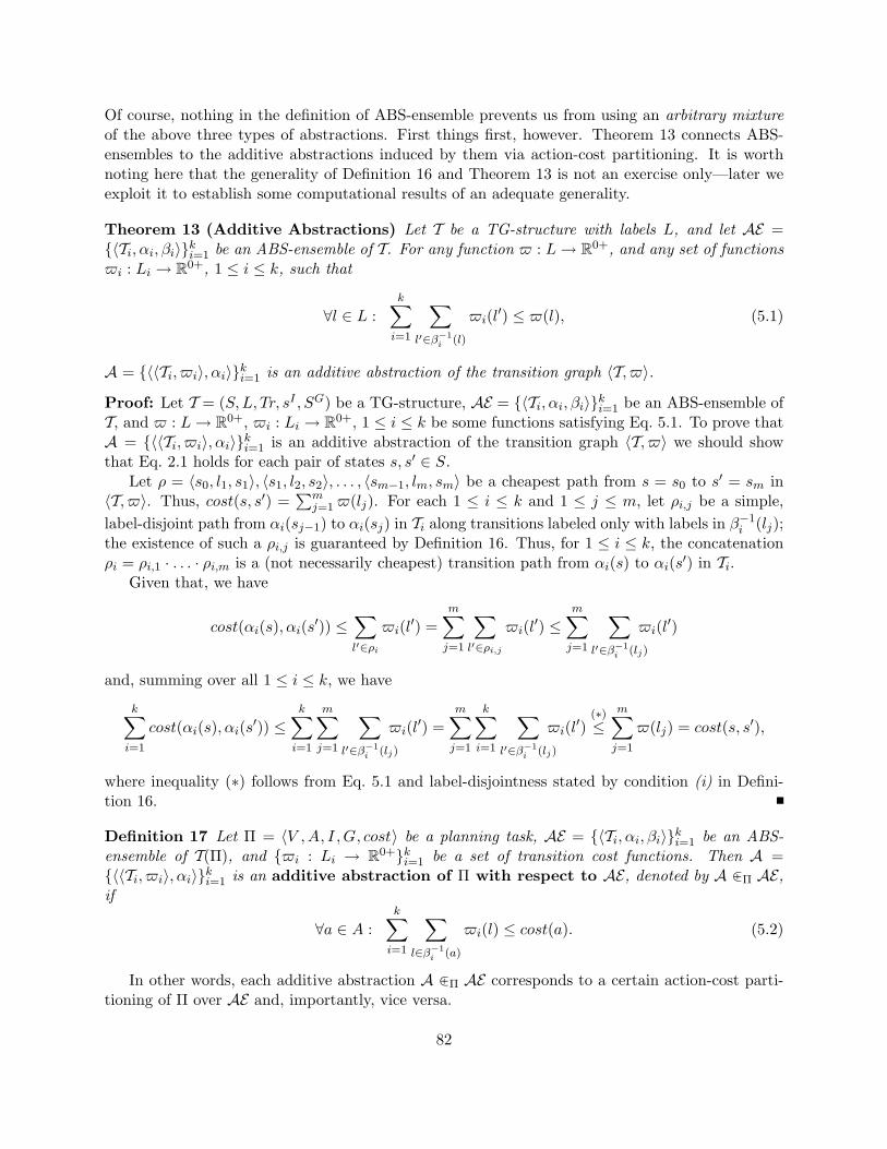
Of course, nothing in the definition of ABS-ensemble prevents us from using an arbitrary mixtureof the above three types of abstractions. First things first, however. Theorem 13 connects ABS-ensembles to the additive abstractions induced by them via action-cost partitioning. It is worthnoting here that the generality of Definition 16 and Theorem 13 is not an exercise only—later weexploit it to establish some computational results of an adequate generality.
Theorem 13 (Additive Abstractions) Let T be a TG-structure with labels L, and let AE ={〈Ti, αi, βi〉}ki=1 be an ABS-ensemble of T. For any function $ : L→ R0+, and any set of functions$i : Li → R0+, 1 ≤ i ≤ k, such that
∀l ∈ L :k∑i=1
∑l′∈β−1
i (l)
$i(l′) ≤ $(l), (5.1)
A = {〈〈Ti, $i〉, αi〉}ki=1 is an additive abstraction of the transition graph 〈T, $〉.Proof: Let T = (S,L, Tr, sI , SG) be a TG-structure, AE = {〈Ti, αi, βi〉}ki=1 be an ABS-ensemble ofT, and $ : L→ R0+, $i : Li → R0+, 1 ≤ i ≤ k be some functions satisfying Eq. 5.1. To prove thatA = {〈〈Ti, $i〉, αi〉}ki=1 is an additive abstraction of the transition graph 〈T, $〉 we should showthat Eq. 2.1 holds for each pair of states s, s′ ∈ S.
Let ρ = 〈s0, l1, s1〉, 〈s1, l2, s2〉, . . . , 〈sm−1, lm, sm〉 be a cheapest path from s = s0 to s′ = sm in〈T, $〉. Thus, cost(s, s′) =
∑mj=1$(lj). For each 1 ≤ i ≤ k and 1 ≤ j ≤ m, let ρi,j be a simple,
label-disjoint path from αi(sj−1) to αi(sj) in Ti along transitions labeled only with labels in β−1i (lj);
the existence of such a ρi,j is guaranteed by Definition 16. Thus, for 1 ≤ i ≤ k, the concatenationρi = ρi,1 · . . . · ρi,m is a (not necessarily cheapest) transition path from αi(s) to αi(s′) in Ti.
Given that, we have
cost(αi(s), αi(s′)) ≤∑l′∈ρi
$i(l′) =m∑j=1
∑l′∈ρi,j
$i(l′) ≤m∑j=1
∑l′∈β−1
i (lj)
$i(l′)
and, summing over all 1 ≤ i ≤ k, we have
k∑i=1
cost(αi(s), αi(s′)) ≤k∑i=1
m∑j=1
∑l′∈β−1
i (lj)
$i(l′) =m∑j=1
k∑i=1
∑l′∈β−1
i (lj)
$i(l′)(∗)≤
m∑j=1
$(lj) = cost(s, s′),
where inequality (∗) follows from Eq. 5.1 and label-disjointness stated by condition (i) in Defini-tion 16.
Definition 17 Let Π = 〈V ,A, I ,G, cost〉 be a planning task, AE = {〈Ti, αi, βi〉}ki=1 be an ABS-ensemble of T(Π), and {$i : Li → R0+}ki=1 be a set of transition cost functions. Then A ={〈〈Ti, $i〉, αi〉}ki=1 is an additive abstraction of Π with respect to AE, denoted by A AΠ AE,if
∀a ∈ A :k∑i=1
∑l∈β−1
i (a)
$i(l) ≤ cost(a). (5.2)
In other words, each additive abstraction A AΠ AE corresponds to a certain action-cost parti-tioning of Π over AE and, importantly, vice versa.
82
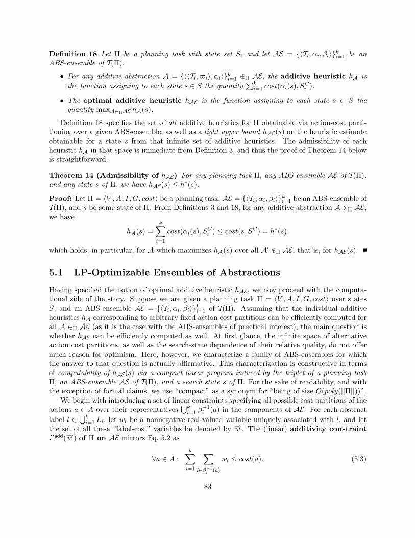
Definition 18 Let Π be a planning task with state set S, and let AE = {〈Ti, αi, βi〉}ki=1 be anABS-ensemble of T(Π).
• For any additive abstraction A = {〈〈Ti, $i〉, αi〉}ki=1 AΠ AE, the additive heuristic hA isthe function assigning to each state s ∈ S the quantity
∑ki=1 cost(αi(s), S
Gi ).
• The optimal additive heuristic hAE is the function assigning to each state s ∈ S thequantity maxAAΠAE hA(s).
Definition 18 specifies the set of all additive heuristics for Π obtainable via action-cost parti-tioning over a given ABS-ensemble, as well as a tight upper bound hAE(s) on the heuristic estimateobtainable for a state s from that infinite set of additive heuristics. The admissibility of eachheuristic hA in that space is immediate from Definition 3, and thus the proof of Theorem 14 belowis straightforward.
Theorem 14 (Admissibility of hAE) For any planning task Π, any ABS-ensemble AE of T(Π),and any state s of Π, we have hAE(s) ≤ h∗(s).Proof: Let Π = 〈V ,A, I ,G, cost〉 be a planning task, AE = {〈Ti, αi, βi〉}ki=1 be an ABS-ensemble ofT(Π), and s be some state of Π. From Definitions 3 and 18, for any additive abstraction A AΠ AE,we have
hA(s) =k∑i=1
cost(αi(s), SGi ) ≤ cost(s, SG) = h∗(s),
which holds, in particular, for A which maximizes hA(s) over all A′ AΠ AE, that is, for hAE(s).
5.1 LP-Optimizable Ensembles of Abstractions
Having specified the notion of optimal additive heuristic hAE , we now proceed with the computa-tional side of the story. Suppose we are given a planning task Π = 〈V ,A, I ,G, cost〉 over statesS, and an ABS-ensemble AE = {〈Ti, αi, βi〉}ki=1 of T(Π). Assuming that the individual additiveheuristics hA corresponding to arbitrary fixed action cost partitions can be efficiently computed forall A AΠ AE (as it is the case with the ABS-ensembles of practical interest), the main question iswhether hAE can be efficiently computed as well. At first glance, the infinite space of alternativeaction cost partitions, as well as the search-state dependence of their relative quality, do not offermuch reason for optimism. Here, however, we characterize a family of ABS-ensembles for whichthe answer to that question is actually affirmative. This characterization is constructive in termsof computability of hAE(s) via a compact linear program induced by the triplet of a planning taskΠ, an ABS-ensemble AE of T(Π), and a search state s of Π. For the sake of readability, and withthe exception of formal claims, we use “compact” as a synonym for “being of size O(poly(||Π||))”.
We begin with introducing a set of linear constraints specifying all possible cost partitions of theactions a ∈ A over their representatives
⋃ki=1 β
−1i (a) in the components of AE. For each abstract
label l ∈ ⋃ki=1 Li, let wl be a nonnegative real-valued variable uniquely associated with l, and let
the set of all these “label-cost” variables be denoted by −→w . The (linear) additivity constraintCadd(−→w ) of Π on AE mirrors Eq. 5.2 as
∀a ∈ A :k∑i=1
∑l∈β−1
i (a)
wl ≤ cost(a). (5.3)
83
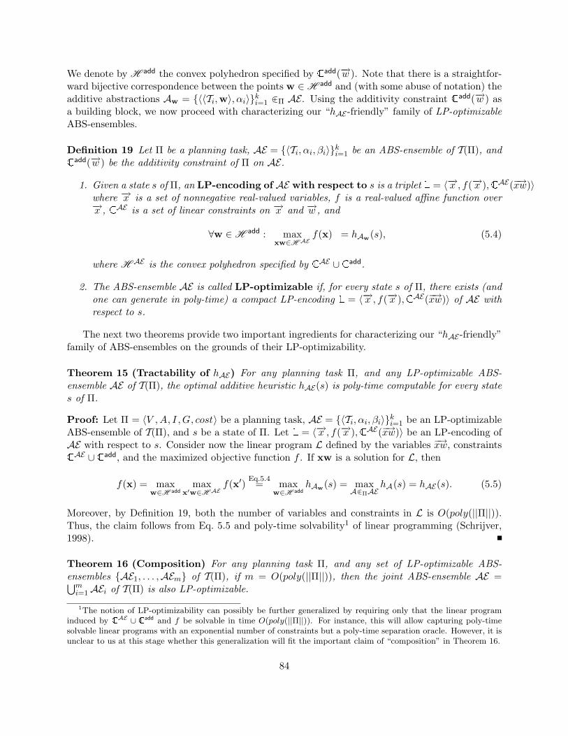
We denote by H add the convex polyhedron specified by Cadd(−→w ). Note that there is a straightfor-ward bijective correspondence between the points w ∈H add and (with some abuse of notation) theadditive abstractions Aw = {〈〈Ti,w〉, αi〉}ki=1 AΠ AE. Using the additivity constraint Cadd(−→w ) asa building block, we now proceed with characterizing our “hAE-friendly” family of LP-optimizableABS-ensembles.
Definition 19 Let Π be a planning task, AE = {〈Ti, αi, βi〉}ki=1 be an ABS-ensemble of T(Π), andCadd(−→w ) be the additivity constraint of Π on AE.
1. Given a state s of Π, an LP-encoding of AE with respect to s is a triplet L = 〈−→x , f(−→x ),CAE(−→xw)〉where −→x is a set of nonnegative real-valued variables, f is a real-valued affine function over−→x , CAE is a set of linear constraints on −→x and −→w , and
∀w ∈H add : maxxw∈H AE
f(x) = hAw(s), (5.4)
where H AE is the convex polyhedron specified by CAE ∪ Cadd.
2. The ABS-ensemble AE is called LP-optimizable if, for every state s of Π, there exists (andone can generate in poly-time) a compact LP-encoding L = 〈−→x , f(−→x ),CAE(−→xw)〉 of AE withrespect to s.
The next two theorems provide two important ingredients for characterizing our “hAE-friendly”family of ABS-ensembles on the grounds of their LP-optimizability.
Theorem 15 (Tractability of hAE) For any planning task Π, and any LP-optimizable ABS-ensemble AE of T(Π), the optimal additive heuristic hAE(s) is poly-time computable for every states of Π.
Proof: Let Π = 〈V ,A, I ,G, cost〉 be a planning task, AE = {〈Ti, αi, βi〉}ki=1 be an LP-optimizableABS-ensemble of T(Π), and s be a state of Π. Let L = 〈−→x , f(−→x ),CAE(−→xw)〉 be an LP-encoding ofAE with respect to s. Consider now the linear program L defined by the variables −→xw, constraintsCAE ∪ Cadd, and the maximized objective function f . If xw is a solution for L, then
f(x) = maxw∈H add
maxx′w∈H AE
f(x′)Eq.5.4
= maxw∈H add
hAw(s) = maxAAΠAE
hA(s) = hAE(s). (5.5)
Moreover, by Definition 19, both the number of variables and constraints in L is O(poly(||Π||)).Thus, the claim follows from Eq. 5.5 and poly-time solvability1 of linear programming (Schrijver,1998).
Theorem 16 (Composition) For any planning task Π, and any set of LP-optimizable ABS-ensembles {AE1, . . . ,AEm} of T(Π), if m = O(poly(||Π||)), then the joint ABS-ensemble AE =⋃mi=1AEi of T(Π) is also LP-optimizable.
1The notion of LP-optimizability can possibly be further generalized by requiring only that the linear programinduced by CAE ∪ Cadd and f be solvable in time O(poly(||Π||)). For instance, this will allow capturing poly-timesolvable linear programs with an exponential number of constraints but a poly-time separation oracle. However, it isunclear to us at this stage whether this generalization will fit the important claim of “composition” in Theorem 16.
84
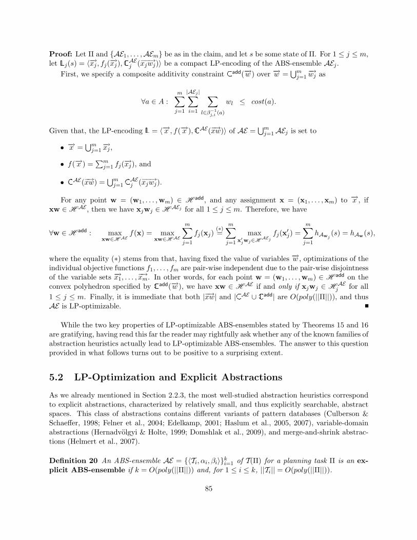
Proof: Let Π and {AE1, . . . ,AEm} be as in the claim, and let s be some state of Π. For 1 ≤ j ≤ m,let Lj(s) = 〈−→xj , fj(−→xj),CAEj (−−→xjwj)〉 be a compact LP-encoding of the ABS-ensemble AEj .
First, we specify a composite additivity constraint Cadd(−→w ) over −→w =⋃mj=1−→wj as
∀a ∈ A :m∑j=1
|AEj |∑i=1
∑l∈β−1
j,i (a)
wl ≤ cost(a).
Given that, the LP-encoding L = 〈−→x , f(−→x ),CAE(−→xw)〉 of AE =⋃mj=1AEj is set to
• −→x =⋃mj=1−→xj ,
• f(−→x ) =∑m
j=1 fj(−→xj), and
• CAE(−→xw) =⋃mj=1C
AEj (−−→xjwj).
For any point w = (w1, . . . ,wm) ∈ H add, and any assignment x = (x1, . . . ,xm) to −→x , ifxw ∈H AE , then we have xjwj ∈H AEj for all 1 ≤ j ≤ m. Therefore, we have
∀w ∈H add : maxxw∈H AE
f(x) = maxxw∈H AE
m∑j=1
fj(xj)(∗)=
m∑j=1
maxx′jwj∈H AEj
fj(x′j) =m∑j=1
hAwj(s) = hAw(s),
where the equality (∗) stems from that, having fixed the value of variables −→w , optimizations of theindividual objective functions f1, . . . , fm are pair-wise independent due to the pair-wise disjointnessof the variable sets −→x1, . . . ,
−→xm. In other words, for each point w = (w1, . . . ,wm) ∈ H add on theconvex polyhedron specified by Cadd(−→w ), we have xw ∈ H AE if and only if xjwj ∈ H AE
j for all1 ≤ j ≤ m. Finally, it is immediate that both |−→xw| and |CAE ∪ Cadd| are O(poly(||Π||)), and thusAE is LP-optimizable.
While the two key properties of LP-optimizable ABS-ensembles stated by Theorems 15 and 16are gratifying, having read this far the reader may rightfully ask whether any of the known families ofabstraction heuristics actually lead to LP-optimizable ABS-ensembles. The answer to this questionprovided in what follows turns out to be positive to a surprising extent.
5.2 LP-Optimization and Explicit Abstractions
As we already mentioned in Section 2.2.3, the most well-studied abstraction heuristics correspondto explicit abstractions, characterized by relatively small, and thus explicitly searchable, abstractspaces. This class of abstractions contains different variants of pattern databases (Culberson &Schaeffer, 1998; Felner et al., 2004; Edelkamp, 2001; Haslum et al., 2005, 2007), variable-domainabstractions (Hernadvolgyi & Holte, 1999; Domshlak et al., 2009), and merge-and-shrink abstrac-tions (Helmert et al., 2007).
Definition 20 An ABS-ensemble AE = {〈Ti, αi, βi〉}ki=1 of T(Π) for a planning task Π is an ex-plicit ABS-ensemble if k = O(poly(||Π||)) and, for 1 ≤ i ≤ k, ||Ti|| = O(poly(||Π||)).
85
For any explicit ABS-ensemble AE, any explicit abstraction A = {〈〈Ti, $i〉, αi〉}ki=1 AΠ AEinduces an admissible additive heuristic hA . So far, however, how to choose this abstraction, thatis, the actual choice of the action-cost partitioning, has remained an open issue, and the choiceswere made on an ad hoc basis (Yang et al., 2007). This is exactly where LP-optimization comesinto the picture.
Computing hA =∑k
i=1 cost(αi(s), SGi ) for a fixed explicit abstractionA = {〈〈Ti, $i〉, αi〉}ki=1 AΠ
AE is usually done by computing each cost(αi(s), SGi ) using either breadth-first search or the Dijk-stra algorithm over the explicitly constructed transition graph 〈Ti, $i〉. However, the correspondingsingle-source shortest paths (SSSP) problem also has an elegant LP formulation. Given a directedgraph G = (N,E) and a source node v ∈ N , if d(v′) is a variable corresponding to the shortest-pathlength from v to v′, then the solution of the linear program
max−→d
∑v′
d(v′)
s.t. d(v) = 0d(v′′) ≤ d(v′) + w(v′, v′′), ∀(v′, v′′) ∈ E
(5.6)
induces a solution to the SSSP problem over G and source v.The LP formulation of the SSSP problem is not widely used as the aforementioned graph-search
techniques resolve SSSP much more efficiently. However, this LP formulation is precisely what weneed to bridge the gap between explicit abstractions and optimal action cost partition. A compactLP-encoding of an explicit ABS-ensemble AE = {〈Ti, αi, βi〉}ki=1 can now be obtained by
(1) putting together the linear constraints as in Eq. 5.6 for TG-structures Ti,
(2) replacing the edge-weight constants w(v′, v′′) by variables associated with the correspondingtransition labels, and
(3) constraining the latter label-cost variables with the proper additivity constraints.
Given a planning task Π, an explicit ABS-ensemble AE = {〈Ti, αi, βi〉}ki=1 of T(Π), and a states of Π, the LP-encoding L = 〈−→x , f(−→x ),CAE(−→xw)〉 of AE with respect to s is constructed as follows.First, let the label-cost variables −→w contain a variable wl for every abstract label l ∈ ⋃k
i=1 Li. Theadditivity constraint is defined in terms of these label-cost variables −→w exactly as in Eq. 5.3. Thecomponents of the LP-encoding L are then set to
−→x =k⋃i=1
{d(σ) | σ ∈ Si} ∪ {d(Gi)}
CAE =
d(σ) ≤ d(σ′) + wl, ∀〈σ′, l, σ〉 ∈ Trid(σ) = 0, σ = αi(s)d(Gi) ≤ d(σ), σ ∈ SGi
, ∀i
f(−→x ) =k∑i=1
d(Gi).
(5.7)
Since each TG-structure Ti in explicit ABS-ensemble AE is of size O(poly(||Π||)), it is immediatethat the LP-encoding L = 〈−→x , f(−→x ),CAE(−→xw)〉 is both compact and poly-time constructible forany state s of Π, giving us all we need to prove Theorem 17 below.
86
Theorem 17 Optimal additive heuristic hAE(s) is poly-time computable for any planning task Π,any explicit ABS-ensemble AE, and any state s of Π.
Proof: Let Π be a planning task, AE = {〈Ti, αi, βi〉}ki=1 be an explicit ABS-ensemble of T(Π), s besome state of Π, L = 〈−→x , f(−→x ),CAE(−→xw)〉 be as in Eq. 5.7, and w be some point in H add. Giventhat, we have Aw = {〈〈Ti,w〉, αi〉}ki=1 AΠ AE, and hAw(s) =
∑ki=1 cost(αi(s), S
Gi ). Now, for each
1 ≤ i ≤ k we havemax
xw∈H AEd(Gi) = cost(αi(s), SGi ),
and from disjointness of the constraints for 1 ≤ i 6= i′ ≤ k, we obtain
maxxw∈H AE
f(x) = maxxw∈H AE
k∑i=1
d(Gi) =k∑i=1
maxxw∈H AE
d(Gi) =k∑i=1
cost(αi(s), SGi ) = hAw(s).
From Definition 19 we thus have L = 〈−→x , f(−→x ),CAE(−→xw)〉 being an LP-encoding ofAE = {〈Ti, αi, βi〉}ki=1
with respect to s. In turn, by Definition 20,∑k
i=1 ||Ti|| = O(poly(||Π||)), and hence L is both com-pact and poly-time constructible, finalizing the proof of the claim.
5.3 LP-Optimization and Implicit Abstractions I: Fork Decompo-sition
Explicit abstractions are clearly the most well-known abstractions in the context of heuristic searchin general, and planning as heuristic search in particular. Recently, however, Katz and Domshlak(2008c, 2009b) introduced the concept of implicit abstraction heuristics corresponding to certainimplicit abstractions of planning tasks at hand. The basic idea behind implicit abstractions is inabstracting the task at hand into instances of provably tractable fragments of optimal planning.This, in particular, abolishes the limitation of explicit abstractions to use fixed-size abstract spacesonly. Concretizing the idea of implicit abstractions, Katz and Domshlak (2008c) introduced aconcrete framework based on decomposing the planning task along its causal graph and proposeda concrete instance of this framework, called fork-decomposition. Fork-decomposition (additive)abstraction is based on two specific fragments of tractable cost-optimal planning. For the technicaldetails of fork decomposition in full we refer the reader to Katz and Domshlak (2008c). For ourpurposes here, it suffices to say that a fork decomposition of a planning task Π = 〈V ,A, I ,G, cost〉over states S is obtained as follows.
(1) Schematic construction of a set of projection abstractions Π = {Παfv ,Παi
v}v∈V with each V αfv =
{v} ∪ succ(v) and V αiv = {v} ∪ pred(v). Note that, unlike explicit abstractions, each abstract
space Sαfv and Sα
iv can be of size Θ(|S|).
(2) Reformulation of the actions within the abstractions to single-effect actions only, so that thecausal graphs of Παf
v and Παiv become, respectively, “forks” and “inverted forks” rooted in v.
After this action reformulation, the individual abstractions may cease being purely homomor-phic.
(3) Within each Παfv , arbitrary abstraction of the domain of v to {0, 1}, and within each Παi
v ,arbitrary abstraction of the domain of v to {0, 1, . . . , k} with k = O(1).
87
This decomposition of Π provides us with the fork-decomposition ABS-ensemble AE ={〈T(Παf
v), αfv, β
fv〉, 〈T(Παi
v), αiv, β
iv〉}v∈V of T(Π), with the action associations βf
v, βiv being established
along the above steps (1-3). The additive abstractions of such an ABS-ensemble AE are of interestbecause (i) they can provide very informative heuristic estimates (Katz & Domshlak, 2009b), and(ii) each abstract task in Π = {Παf
v ,Παiv}v∈V can be solved in polynomial time by special-purpose
algorithms for the corresponding fragments of sas+ (Katz & Domshlak, 2008c). However, here aswell, the choice of abstraction A AΠ AE with respect to AE is important, and optimizing this choiceis clearly desirable. Interestingly, LP-optimization can come to the rescue here as well, despite ourinability to perform an explicit search of TG-structures of AE in polynomial time.
Theorem 18 For any planning task Π, any fork-decomposition ABS-ensemble of T(Π) is LP-optimizable, and thus hAE(s) is poly-time computable for every state s of Π.
Proof: From Lemmas 6 and 7 below, for each v ∈ V , we have each AE fv = {〈T(Παf
v), αfv, β
fv〉} and
each AE ii = {〈T(Παi
v), αiv, β
iv〉} being LP-optimizable. From the composition Theorem 16, we thus
have AE being LP-optimizable.
Lemma 6 For any planning task Π = 〈V ,A, I ,G, cost〉 and any variable r ∈ V , the “single fork”ABS-ensemble AE f
r = {〈T(Παfr), αf
r, βfr〉} of T(Π) is LP-optimizable.
Proof: Given a planning task Π = 〈V ,A, I ,G, cost〉 and a variable r ∈ V , letAE fr = {〈T(Παf
r), αfr, β
fr〉}
be a fork-decomposition of T(Π) over a single fork rooted in a binary domain variable r, and s besome state of Π. Our LP-encoding of such a “single fork” ABS-ensemble AE f
r with respect to s cor-responds to an LP reformulation of the polynomial-time algorithm of Katz and Domshlak (2008c)for fork-structured tasks with binary root domain.
To simplify the notation, let us denote the variables V αfr of our fork-structured abstract task
by V ′, its actions by A′, its goal state by G′, and the abstraction αfr(s) of the state s in question
by s′. We can assume that G′[v] is defined for all v ∈ V ′ \ {r}; all the goal-less leaves can simplybe omitted from the fork. For compliance with the notation of Katz and Domshlak (2008c), wedenote the (abstracted to binary-valued) domain of r by D(r) = {0, 1} such that s′[r] = 0. Letσ(r) be a 0/1 sequence of length 1 + maxv∈V ′ |D(v)|, and, for 1 ≤ i ≤ |σ(r)|, σ(r)[i] = 0 if i is odd,and = 1, if i is even. Let �∗[σ(r)] be the set of all nonempty prefixes of σ(r) if G′[r] is unspecified;otherwise let it be the set of all prefixes of σ(r) ending with G′[r]. In what follows, for each of thetwo root’s values ϑ ∈ D(r), ¬ϑ denotes the opposite value 1 − ϑ. Let DTGϑrv be the subgraph ofDTG(v,Παf
r) obtained by removing from the latter all the arcs labeled with r = ¬ϑr.To facilitate the presentation, the algorithm for fork-structured tasks Π′ = 〈V ′, A′, s′, G′, cost′〉
with binary root domain (Katz & Domshlak, 2008c) appears here as it appeared in the proof ofTheorem 11.
(i) For each of the two values ϑr ∈ D(r) of the root variable, each leaf variable v ∈ V ′ \ {r}, andeach pair of values ϑ, ϑ′ ∈ D(v), let pϑ,ϑ′;ϑr be the cost of the cheapest sequence of actions ϑto ϑ′ provided r = ϑr. The whole set {pϑ,ϑ′;ϑr} can be computed by a straightforward variantof the all-pairs-shortest-paths Floyd-Warshall algorithm on DTGϑr
v in time O(d3|V |).
(ii) For each leaf v ∈ V ′ \ {r}, 1 ≤ i ≤ d + 1, and ϑ ∈ D(v), let gϑ;i be the cost of the cheapestsequence of actions changing s′[v] to ϑ provided a sequence σ ∈ �∗[σ(r)], |σ| = i, of value
88
changes of r. Given {pϑ,ϑ′;ϑr} as in (i), the set {gϑ;i} is given by the solution of the recursiveequation
gϑ;i =
ps′[v],ϑ;s′[r], i = 1minϑ′
gϑ′;i−1 + pϑ′,ϑ;s′[r], 1 < i ≤ δϑ, i is odd
minϑ′
gϑ′;i−1 + pϑ′,ϑ;¬s′[r], 1 < i ≤ δϑ, i is even
gϑ;i−1, δϑ < i ≤ d+ 1
,
where δϑ = |D(v)|+ 1.
(iii) Given that,
h∗(s′) = minσ∈�∗[σ(r)]
cost′(σ) +∑
v∈V ′\{r}
gG′[v];|σ|
.Our LP-encoding reformulates the algorithm as follows. First, we set the label-cost variables
−→w to contain a variable wa for each abstract action a ∈ A′; the additivity constraints Cadd(−→w ) aredefined in terms of these label-cost variables via βf
r as in Eq. 5.3. Now we specify the LP-encodingL = 〈−→x , f(−→x ),CAE(−→xw)〉 of AE f
r with respect to s as follows. The variable set −→x of L consists ofthree types of variables, notably
−→x = {hf} ∪⋃
v∈V ′\{r},ϑ∈D(v),
1≤i≤|σ(r)|
{d(v, ϑ, i)} ∪⋃
v∈V ′\{r},ϑ,ϑ′∈D(v),ϑr∈{0,1}
{p(v, ϑ, ϑ′, ϑr)}.
• The variable hf stands for the minimal cost of solving our fork-structured planning task, andthe maximized objective function of L is simply f(−→x ) = hf .
• Each variable d(v, ϑ, i) stands for the cost of the cheapest sequence of actions affecting v thatchanges its value from s′[v] to ϑ given that the value changes of r induce a 0/1 sequence ofr’s values of length i.
• Each variable p(v, ϑ, ϑ′, ϑr) stands for the cost of the cheapest sequence of actions affecting vthat changes its value from ϑ to ϑ′ having fixed the value of r to ϑr.
The constraint set CAE of L consists of the following sets of linear constraints.
(i) For each v ∈ V ′ \ {r}, ϑ ∈ D(v),
p(v, ϑ, ϑ, 0) = 0, p(v, ϑ, ϑ, 1) = 0.
Likewise, for each v-changing action a ∈ A′ and each ϑr ∈ Pre(a)[r], if v ∈ V(pre(a)), then
p(v, ϑ, eff(a)[v], ϑr) ≤ p(v, ϑ, pre(a)[v], ϑr) + wa
and otherwise,p(v, ϑ, eff(a)[v], ϑr) ≤ wa.
Semantics: Shortest-path constraints as in Eq. 5.6.
89
(ii) For each leaf v ∈ V ′ \ {r} and each ϑ ∈ D(v)
d(v, ϑ, 1) ≤ p(v, s′[v], ϑ, σ(r)[1])
and, for each ϑ′ ∈ D(v), and 1 < i ≤ |σ(r)|,
d(v, ϑ, i) ≤ d(v, ϑ′, i− 1) + p(v, ϑ′, ϑ, σ(r)[i])
Semantics: The cost of achieving ϑ from s′[v] given |σ(r)| = i is bounded by the cost ofachieving ϑ′ given |σ(r)| = i− 1, and achieving ϑ from ϑ′ given σ(r)[i].
(iii) For all goal-achieving sequences σ ∈ �∗[σ(r)] of value changes of r, and each pair of r-changingactions a, a′ ∈ A′ such that eff(a)[r] = 1 and eff(a′)[r] = 0,
hf ≤ d|σ| − 12e · wa + b |σ| − 1
2c · wa′ +
∑v∈V ′\{r}
d(v,G′[v], |σ|)
Semantics: The cost of solving the task is not greater than the sum of achieving the goalvalues for all the leaves given a value sequence of the root, plus the cost of providing thatvalue sequence.
This finalizes our LP-encoding for an ABS-ensemble consisting of a single fork-structured ab-straction with a binary root domain. Let w be an arbitrary point in H add and let the actioncost function cost′ be set according to w. That is, for each a ∈ A′, cost′(a) = w[wa]. Let vec-tor x ∈ D(−→x ) be specified according to the values obtained while running Katz and Domshlak’salgorithm on Π′ = 〈V ′, A′, s′, G′, cost′〉 as follows.
x[p(v, ϑ, ϑ′, ϑr)] = pϑ,ϑ′;ϑr ,
x[d(v, ϑ, i)] = gϑ;i
x[hf ] = minσ∈�∗[σ(r)]
cost′(σ) +∑
v∈V ′\{r}
gG′[v];|σ|
.Note that constraint sets (i), (ii), and (iii), respectively, reformulate steps (i), (ii), and (iii) ofthe algorithm while keeping the action costs as free variables {wa}. Hence, xw agrees with theconstraint sets (i), (ii), and (iii), and thus xw ∈H AE , implying
maxxw∈H AE
hf ≥ x[hf ] = h∗(s′).
For the other direction, let x ∈ D(−→x ) be such that xw ∈ H AE , σ ∈ �∗[σ(r)] be the oneresponsible for the minimum found by the algorithm for the planning task Π′ = 〈V ′, A′, s′, G′, cost′〉,and let ρ be an optimal plan for Π′ such that ρ↓r induces σ. For each v ∈ V ′ \ {r}, let ρ↓v=ρ1, . . . , ρm, 1 ≤ m ≤ |σ| be the sequence of actions changing the values of v, split by executionof r-changing actions ρ↓r along ρ. Each such ρi = 〈ai1 . . . aiki〉 is a sequence of actions inducinga sequence of v-values ϑi0, ϑ
i1, . . . , ϑ
iki
, and ϑ10, ϑ
11, . . . , ϑ
1k1, ϑ2
1, . . . , ϑ2k2, . . . , ϑm1 , . . . , ϑ
mkm
is a simplepath from s′[v] = ϑ1
0 to G′[v] = ϑmkm in the domain transition graph of v such that, for 1 ≤ i ≤ m,
90
the change to ϑij , 1 ≤ j ≤ ki is labeled by either σ[i] or nothing at all. For ease of presentation, foreach 1 ≤ i ≤ m we denote ϑi+1
0 = ϑiki . Given that,
x[d(v,G′[v], |σ|)](ii)
≤m∑i=1
ki∑j=1
x[p(v, ϑij−1, ϑij , σ[i])]
(i)
≤m∑i=1
ki∑j=1
w[aij ] = cost′(ρ↓v),
and thus
x[hf ](iii)
≤∑a∈ρ↓r
w[a] +∑
v∈V ′\{r}
x[d(v,G′[v], |σ|)] ≤ cost′(ρ↓r) +∑
v∈V ′\{r}
cost′(ρ↓v) = cost′(ρ),
implyingmax
xw∈H AEhf ≤ h∗(s′).
Putting the two directions together, for each w ∈H add, we have
maxxw∈H AE
f(x) = hAw(s),
and from Definition 19 we thus have L = 〈−→x , f(−→x ),CAE(−→xw)〉 being an LP-encoding of AE fr. Note
that if D = maxv∈V ′ |D(v)|, then the LP variable set size |−→x | is O(|V | ·D2) and the constraint setsize |CAE | is O(D · |A′|2 + |V ′| ·D3 + |A′| · |V ′| ·D), and thus the LP-encoding is compact.
Lemma 7 For any planning task Π = 〈V ,A, I ,G, cost〉 and any variable r ∈ V , the “singleinverted fork” ABS-ensemble AE i
r = {〈T(Παir), αi
r, βir〉} of T(Π) is LP-optimizable.
Proof: Given a planning task Π = 〈V ,A, I ,G, cost〉 and a variable r ∈ V , letAE ir = {〈T(Παi
r), αir, β
ir〉}
be a fork-decomposition of T(Π) over a single inverted fork with sink r, and let s be some stateof Π. Our LP-encoding of such a “single inverted fork” ABS-ensemble AE i
r with respect to states corresponds to an LP reformulation of the polynomial-time algorithm of Katz and Domshlak(2008c) for inverted-fork structured tasks with root domain of size O(1).
As in the proof of Lemma 6, let us denote the variables V αir of our inverted-fork structured
abstract task by V ′, its actions by A′, its goal state by G′, and the abstraction αir(s) of the state
s in question by s′. First, we set the label-cost variables −→w to contain a variable wa for everyabstract action a ∈ A′; the additivity constraints Cadd(−→w ) are then defined in terms of these label-cost variables via βi as in Eq. 5.3. To facilitate the presentation, the algorithm for inverted-forkstructured tasks Π′ = 〈V ′, A′, s′, G′, cost′〉 with sink domain of size O(1) (Katz & Domshlak, 2008c)appears here as it appeared in the proof of Theorem 12.
(i) For each parent variable v ∈ V ′ \ {r}, and each pair of its values ϑ, ϑ′ ∈ D(v), let pϑ,ϑ′ bethe cost of the cheapest sequence of actions changing ϑ to ϑ′. The whole set {pϑ,ϑ′} can becomputed using the Floyd-Warshall algorithm on the domain transition graph of v in timeO(d3|V |).
91
(ii) For each cycle-free path π = a1 · . . . · am from s′[r] to G′[r] in DTG(r,Π′), let gπ be the costof the cheapest plan from s′ in Π′ based on π, and the shortest paths computed in (1). Eachgπ can be computed as
gπ =m∑i=1
cost(ai) +m∑i=0
∑v∈V ′\{r}
pprei[v],prei+1[v],
where {pre0 · . . . · prem+1} are the values needed from the parents of r along the path π. Thatis, for each v ∈ V ′ \ {r}, and 0 ≤ i ≤ m+ 1,
prei[v] =
s′[v], i = 0G′[v], i = m+ 1, and G′[v] is specifiedpre(ai)[v], 1 ≤ i ≤ m, and pre(ai)[v] is specifiedprei−1[v] otherwise
. (5.8)
From that, we have h∗(s′) = minπ gπ.
Given that any optimal plan for Π′ must correspond to a cycle-free path in DTG(r,Π′) froms′[r] to G′[r], our LP-encoding L = 〈−→x , f(−→x ),CAE(−→xw)〉 of AE with respect to state s reformulatesthe algorithm as follows. The variable set −→x of L consists of two types of variables, notably
−→x = {hi} ∪⋃
v∈V ′\{r},ϑ,ϑ′∈D(v)
{d(v, ϑ, ϑ′)}.
• The variable hi stands for the minimal cost of solving our inverted fork-structured planningtask, and the maximized objective function of L is simply f(−→x ) = hi.
• Each variable d(v, ϑ, ϑ′) stands for the cost of the cheapest sequence of actions affecting vthat changes its value from ϑ to ϑ′.
The constraint CAE of L consists of the following sets of linear constraints:
(i) For each v ∈ V ′ \ {r} and each ϑ ∈ D(v),
d(v, ϑ, ϑ) = 0.
Likewise, for each v-changing action a ∈ A′, if v ∈ V(pre(a)), then
d(v, ϑ, eff(a)[v]) ≤ d(v, ϑ, pre(a)[v]) + wa
and otherwise,d(v, ϑ, eff(a)[v]) ≤ wa.
Semantics: Shortest-path constraints as in Eq. 5.6.
(ii) For each cycle-free path π = a1 · . . . · am from s′[r] to G′[r] in DTG(r,Π′),
hi ≤m∑i=1
wai +m∑i=0
∑v∈V ′\{r}
d(v, prei[v], prei+1[v])
92
where, for each 0 ≤ i ≤ m+ 1, prei is defined as in Eq. 5.8.
Semantics: The cost of solving the task is not greater than the cost of any cycle-free path ofr plus sums of costs of reaching the prevail conditions of actions on this path and reachingthe goal afterwards.
This finalizes our LP-encoding for an ABS-ensemble consisting of a single inverted-fork struc-tured abstraction with a O(1)-bounded root domain. Let w be an arbitrary point in H add and letthe action cost function cost′ be set according to w. That is, for each a ∈ A′, cost′(a) = w[wa]. Letvector x ∈ D(−→x ) be specified according to the values obtained while running Katz and Domshlak’salgorithm on Π′ = 〈V ′, A′, s′, G′, cost′〉 as follows.
x[d(v, ϑ, ϑ′)] = pϑ,ϑ′ ,
x[hi] = minπgπ.
Note that constraint sets (i) and (ii), respectively, reformulate steps (i) and (ii) of the algorithmwhile keeping the action costs as free variables {wa}. Hence, xw agrees with the constraint sets (i)and (ii), and thus xw ∈H AE , implying
maxxw∈H AE
hi ≥ x[hi] = h∗(s′).
For the other direction, let x ∈ D(−→x ) be such that xw ∈H AE , and let ρ be an optimal plan forthe planning task Π′ = 〈V ′, A′, s′, G′, cost′〉. Let π = a1 · . . . · am be the path from s′[r] to G′[r] inDTG(r,Π′) induced by ρ. Note that π is cycle-free by the optimality of ρ. For each v ∈ V ′ \{r}, letρ↓v= ρ0, . . . , ρm be the sequence of actions changing the values of v, split by execution of r-changingactions of π along ρ. Then each ρi = 〈ai1 . . . aiki〉 is a sequence of actions changing the value of vfrom prei[v] to prei+1[v] as in Eq 5.8, and
m∑i=0
x[d(v, prei[v], prei+1[v])](i)≤
m∑i=0
ki∑j=1
w[waij ] = cost′(ρ↓v).
Hence,
x[hi](ii)≤
m∑i=0
w[wai ] +∑
v∈V ′\{r}
m∑i=0
x[d(v, prei[v], prei+1[v])] ≤ cost′(π) +∑
v∈V ′\{r}
cost′(ρ↓v) = cost′(ρ) = h∗(s′),
implyingmax
xw∈H AEhi ≤ h∗(s′).
Putting the two directions together, for each w ∈H add, we have
maxxw∈H AE
f(x) = hAw(s),
and from Definition 19 we thus have L = 〈−→x , f(−→x ),CAE(−→xw)〉 being an LP-encoding of AE ir. Note
that, if D = maxv∈V ′ |D(v)| and d = |D(r)|, then the LP variable set size |−→x | is O(|V ′| ·D2) andthe constraint set size |CAE | is O(dd+ |V ′| · |A′| ·D), and thus the LP-encoding is compact and AE i
r
is LP-optimizable.
93
5.4 LP-Optimization and Implicit Abstractions II: Tree-structuredCOPs
Fork-decomposition implicit abstractions are grounded in two specific fragments of tractable cost-optimal planning. In principle, however, implicit abstractions based on some other tractable frag-ments might also lead to LP-optimizable ABS-ensembles. Here we consider two such fragmentsrecently characterized by Katz and Domshlak (2008a), namely Pb and P(1) (see Section 3.1).
Katz and Domshlak’s poly-time algorithms for the planning fragments Pb and P(1) differ sub-stantially. However, both correspond to reductions of the planning task to compact, tree-structuredconstraint optimization problems (COPs). This joint property of Pb and P(1) (that might alsohold for some other interesting planning fragments) facilitates our objective of adding Pb- andP(1)-based implicit abstractions to the “hAE-friendly” family of LP-optimizable ABS-ensembles.
Let us start by considering a general, tree-structured constraint optimization problem COP =(X ,F) over finite-domain variables X , functional components F , and the objective min
∑ϕ∈F ϕ(X ).
Fixing an arbitrary rooting of the COP’s constraint network at some r ∈ X , in what follows werefer to that rooted tree of COP via its set of directed edges E = {(x, x′)}, oriented “from the rootto the leaves.” In these terms, we have
F = {ϕx : D(y)×D(x)→ R0+ | (y, x) ∈ E}.
It is well known that tree-structured COPs as above can be solved in low polynomial time bya dynamic-programming-style, message-passing algorithm (Dechter, 2003). But like the Dijkstraand breadth-first search algorithms for solving explicit abstractions, this message-passing algorithmdoes not appear to meet our needs. The good news, however, is that such tree-structured COPscan also be solved via linear programming. While we suspect that this quite straightforward, LPformulation is not new, we found no previous mention of it in the literature.
Given a tree-structured constraint optimization problem COP = (X ,F), its LP formulation isusing a set of nonnegative, real-valued variables
−→c = {hcop} ∪⋃
(x′,x)∈E,x′∈D(x′)
{c(x|x′)},
with the semantics of each variable c(x|x′) being an “optimal solution for the subtree rooted at xgiven that the parent x′ of x takes the value x′”. The actual linear program is then
max−→chcop
s.t. ∀r ∈ D(r) : hcop ≤∑
(r,x)∈E
c(x|r),
∀(x, y) ∈ E, x ∈ D(x), y ∈ D(y) :
c(y|x) ≤∑
(y,z)∈E
c(z|y) + ϕy(x, y),
(5.9)
and its solution induces a solution for COP.
94
Lemma 8 Given a tree-structured constraint optimization problem COP = (X ,F) over finite-domain variables X and functional components F , we have
minx∈D(X )
∑ϕ∈F
ϕ(x) = maxc∈H COP
hcop
where H COP is the convex polyhedron specified by the linear constraints as in Eq. 5.9.
Proof: First, note that
∀x ∈ D(X ) and ∀c ∈H COP, hcop ≤∑(y,z)
ϕz(x) =∑ϕ∈F
ϕ(x).
Thereforemax
c∈H COPhcop ≤ min
x∈D(X )
∑ϕ∈F
ϕ(x).
Let c ∈H COP be an assignment constructed by going over the edges (y, z) of the tree bottomup, and for each y ∈ D(y) setting
c(z|y) = minz∈D(z)
∑(z,z′)
c(z′|z) + ϕz(y, z) (5.10)
and then settinghcop = min
r∈D(r)
∑(r,x)
c(x|r). (5.11)
Let x ∈ D(X ) be the combination of assignments to COP variables that establish the minimum inEq. 5.10-5.11. Then
hcop = minx∈D(X )
∑ϕ∈F
ϕ(x),
and thereforemax
c∈H COPhcop ≥ min
x∈D(X )
∑ϕ∈F
ϕ(x).
With Lemma 8 at hand, we now take two additional steps towards an LP-encoding of ABS-ensembles AE containing implicit abstractions reducible to tree-structured COPs. In each such in-dividual implicit abstraction, each value ϕy(x, y) of each functional component ϕy must be somehowprecomputed from the costs of the planning actions. In our case, however, the costs of the actionsin the abstract tasks are not fixed in advance, but should be established by the LP-optimizationprocess. In what follows, we consider this matter more closely.
Given a planning task Π, let AE = {〈T(Π′), α, β〉} be a single-abstraction ABS-ensemble of T(Π)such that cost-optimal planning for Π′ is reducible to a tree-structured constraint optimizationproblem COPΠ′ . First, suppose that, for any fixed vector of action costs w†, each functional-component value ϕ ≡ ϕy(x, y) corresponds to the solution value of some compact canonical-formlinear program
max fϕ(−−→zϕw)s.t. Aϕ · −−→zϕw ≤ bϕ
−→w ≤ w†(5.12)
95
where Aϕ and bϕ are a matrix and a vector of coefficients, respectively. If so, then, given w†, wecan reformulate the linear program in Eq. 5.9 by
(i) replacing the constants ϕ ≡ ϕy(x, y) by the corresponding affine functions fϕ(−−→zϕw), and
(ii) for each ϕ, adding its linear constraints as in Eq. 5.12.
The extended program is still linear, and we still have
minx∈D(X )
∑ϕ∈F
ϕ(x) = maxczw∈H COP
hcop
where z and w are assignments to −→z =⋃ϕ−→z ϕ and action-cost variables −→w , respectively, and
H COP is the convex polyhedron specified by these extended linear constraints.The extended linear program specified above for implicit abstraction Π′ with COPΠ′ satisfy-
ing Eq. 5.12 provides the basis for the LP-encoding of the corresponding ABS-ensembles AE ={〈T(Π′), α, β〉}. First, as before, let the label-cost variables −→w contain a variable wa for everyabstract action a ∈ A′ of Π′; the additivity constraints Cadd(−→w ) are defined in terms of theselabel-cost variables via β as in Eq. 5.3. Now, given a state s of Π, we specify an LP-encodingL = 〈−→x , f(−→x ),CAE(−→xw)〉 of AE with respect to state s as follows.
• The variable set −→x = −→cz consists of the variables of Eqs. 5.9 and 5.12, and the objective of Lis f(−→x ) = hcop.
• The constraint CAE(−→xw) of L consists of all the linear constraints from Eq. 5.9, as well as theconstraint Aϕ · −−→zϕw ≤ bϕ from Eq. 5.12 for each functional-component value ϕ of COPΠ′ .
This finalizes the desired LP-encoding; extending it to such multiple-abstraction ABS-ensemblesAE = {〈T(Π′i), αi, βi〉}ki=1 (and, again, possibly some other LP-optimizable abstractions) is ensuredby the composition Theorem 16.
Theorem 19 Given a planning task Π, and an ABS-ensemble AE = {〈T(Π′i), αi, βi〉}ki=1 of T(Π), ifcost-optimal planning for each Π′i is poly-time reducible to a compact and tree-structured constraintoptimization problem satisfying Eq. 5.12, and k = O(poly(|Π|)), then AE is LP-optimizable, andthus hAE(s) is poly-time computable for every state s ∈ S.
Proof: Let Π be a planning task, AE = {〈T(Π′i), αi, βi〉}ki=1 be an ABS-ensemble of T(Π) as inthe claim, s be some state of Π, and L = 〈−→x , f(−→x ),CAE(−→xw)〉 be as described above. For anyw ∈ H add, let Aw = {〈〈Ti,w〉, αi〉}ki=1 AΠ AE, and therefore hAw(s) =
∑ki=1 cost(αi(s), S
Gi ).
Note that, since Π′i with initial state αi(s) is poly-time reducible to a compact and tree-structuredconstraint optimization problem COPi = (Xi,Fi) satisfying Eq. 5.12, we have
cost(αi(s), SGi ) = minx∈D(Xi)
∑ϕ∈Fi
ϕ(x).
From Lemma 8 we then have
cost(αi(s), SGi ) = maxxw∈H AE
hcopi ,
96
and therefore
maxxw∈H AE
f(x) =k∑i=1
cost(αi(s), SGi ) = hAw(s).
From Definition 19 we then have L = 〈−→x , f(−→x ),CAE(−→xw)〉 being an LP-encoding of AE. In turn,since k = O(poly(|Π|)) and, for 1 ≤ i ≤ k, cost-optimal planning for each abstract task Π′i ispoly-time reducible to a compact and tree-structured constraint optimization problem satisfyingEq. 5.12, the LP-encoding of AE is both compact and poly-time constructible for any state s of Π.Hence, hAE(s) is poly-time computable for any state s of Π.
Last but not least is, of course, the question of whether the requirement posed by Eq. 5.12 isrelevant to the constraint optimization problems induced by the planning tasks from the knownfragments of tractability. The good news is that Theorems 20 and 21 provide an affirmative answerto this question.
Theorem 20 For any task Π = 〈V ,A, I ,G, cost〉 in Pb, cost-optimal planning for Π is poly-timereducible to a compact and tree-structured constraint optimization problem satisfying Eq. 5.12.
Proof: The proof is based on the algorithm of Katz and Domshlak (2008a) for constructinga constraint optimization problem COPΠ = (X ,F) over tree-structured constraint network, aspresented in Section A.1 and depicted in Figure A.3. Let Π = 〈V ,A, I ,G, cost〉 be a planningtask in Pb, and let COPΠ = (X ,F) be the constraint optimization problem resulting in runnig thealgorithm. For each ϕ ∈ F and each assignment to the scope of ϕ, we define a linear programsatisfying Eq. 5.12 as follows. First, for each planning variable v with pred(v) = ∅, and each of itsgoal-valid (time-stamped) value-changing sequences τ ′ ∈ �∗[τ(v)], the constraints set as in Eq. 5.12corresponding to ϕ = ϕv(τ ′) is
zϕ ≤⌊ |τ ′|
2
⌋· wa +
⌊ |τ ′| − 12
⌋· wa′ ,
for each a, a′ ∈ Av such that eff(a)[v] = 1 and eff(a′)[v] = 0. Next, for each planning variable v withpred(v) = {u1, . . . , uk}, k ≥ 1, each goal-valid value-changing sequence τ ′ ∈ �∗[τ(v)] of v, and eachset of such goal-valid value-changing sequences {τ ′1 ∈ �∗[τ(u1)], . . . , τ ′k ∈ �∗[τ(uk)]} of v’s parents,the constraints set corresponding to ϕ = ϕv(τ ′, τ ′1, . . . , τ
′k) is the set of shortest-path constraints of
the digraph G′e(v) as in Eq. 5.6. The union of all the constraint sets above together with the LPformulation as in Eq. 5.9 results in a linear program satisfying Eq. 5.12.
Theorem 21 For any task Π = 〈V ,A, I ,G, cost〉 in P(1), cost-optimal planning for Π is poly-timereducible to a compact and tree-structured constraint optimization problem satisfying Eq. 5.12.
Proof: The proof is based on the algorithm of Katz and Domshlak (2008a) for constructinga constraint optimization problem COPΠ = (X ,F) over tree-structured constraint network, aspresented in Section A.3 and depicted in Figure A.7. Let Π = 〈V ,A, I ,G, cost〉 be a planning taskin P(1), and let COPΠ = (X ,F) be the constraint optimization problem resulting in runnig thealgorithm. For each ϕ ∈ F and each assignment to the scope of ϕ, we define a linear programsatisfying Eq. 5.12 as follows. The key points is that, for each ϕ ∈ F and for each assignment ϕ tothe scope of ϕ, we can define a linear program satisfying Eq. 5.12 by exploiting the fact that
97
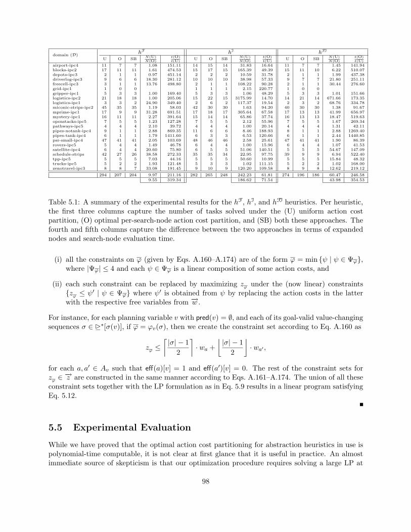
domain (D)hF hI hFI
U O SBN(U)N(O)
t(O)t(U) U O SB
N(U)N(O)
t(O)t(U) U O SB
N(U)N(O)
t(O)t(U)
airport-ipc4 11 7 7 1.08 151.11 14 15 14 31.83 16.64 11 7 7 1.45 141.94blocks-ipc2 17 11 11 1.61 474.53 15 17 15 165.39 49.39 15 11 10 6.22 510.07depots-ipc3 2 1 1 0.97 451.14 2 2 2 10.59 31.78 2 1 1 1.99 437.38driverlog-ipc3 9 6 6 18.30 281.12 10 10 10 38.98 57.33 9 7 7 21.80 251.11freecell-ipc3 3 1 1 13.76 498.80 2 1 1 108.22 90.28 2 1 1 30.44 276.60grid-ipc1 1 0 0 1 1 1 2.15 220.77 1 0 0gripper-ipc1 5 3 3 1.00 169.40 5 3 3 1.06 48.29 5 3 3 1.01 151.66logistics-ipc2 21 18 18 1.00 205.06 15 22 15 3175.99 14.70 14 21 14 671.66 173.35logistics-ipc1 3 3 2 24.90 349.40 2 6 2 117.37 19.54 2 3 2 68.76 334.78miconic-strips-ipc2 45 35 35 1.19 58.03 42 30 30 1.63 94.20 40 30 30 1.38 91.67mprime-ipc1 17 9 9 31.28 691.51 17 18 17 305.64 67.58 17 13 13 41.99 656.97mystery-ipc1 16 11 11 2.27 391.64 15 14 14 65.86 37.74 16 13 13 18.47 519.63openstacks-ipc5 7 5 5 1.23 127.28 7 5 5 2.12 55.96 7 5 5 1.67 269.34pathways-ipc5 4 4 4 2.10 39.72 4 4 4 1.00 20.14 4 4 4 1.31 42.11pipes-notank-ipc4 9 1 1 2.88 869.35 11 6 6 8.46 188.93 8 1 1 2.88 1269.40pipes-tank-ipc4 6 1 1 1.79 1411.60 6 3 3 6.53 120.66 6 1 1 2.44 1440.85psr-small-ipc4 47 41 41 2.05 103.69 48 46 46 2.58 25.61 47 41 41 1.90 86.39rovers-ipc5 5 4 4 1.49 46.78 6 4 4 1.00 15.96 6 4 4 1.07 41.53satellite-ipc4 6 4 4 20.60 75.80 6 5 5 51.06 140.51 5 5 5 54.67 147.09schedule-strips 42 27 26 38.58 272.33 35 35 34 22.95 97.75 39 9 9 6.94 522.40tpp-ipc5 5 5 5 7.03 44.16 5 5 5 50.60 10.99 5 5 5 15.84 48.32trucks-ipc5 5 2 2 1.93 121.48 5 3 3 1.02 111.15 5 2 2 1.02 168.00zenotravel-ipc3 8 8 7 33.08 191.45 9 10 9 120.20 109.58 8 9 8 12.62 219.12
294 207 204 9.97 211.16 282 265 248 242.23 61.81 274 196 186 60.47 246.589.55 319.34 186.62 71.54 43.98 354.53
Table 5.1: A summary of the experimental results for the hF, hI, and hFI heuristics. Per heuristic,the first three columns capture the number of tasks solved under the (U) uniform action costpartition, (O) optimal per-search-node action cost partition, and (SB) both these approaches. Thefourth and fifth columns capture the difference between the two approaches in terms of expandednodes and search-node evaluation time.
(i) all the constraints on ϕ (given by Eqs. A.160–A.174) are of the form ϕ = min {ψ | ψ ∈ Ψϕ},where |Ψϕ| ≤ 4 and each ψ ∈ Ψϕ is a linear composition of some action costs, and
(ii) each such constraint can be replaced by maximizing zϕ under the (now linear) constraints{zϕ ≤ ψ′ | ψ ∈ Ψϕ} where ψ′ is obtained from ψ by replacing the action costs in the latterwith the respective free variables from −→w .
For instance, for each planning variable v with pred(v) = ∅, and each of its goal-valid value-changingsequences σ ∈ �∗[σ(v)], if ϕ = ϕv(σ), then we create the constraint set according to Eq. A.160 as
zϕ ≤⌈ |σ| − 1
2
⌉· wa +
⌊ |σ| − 12
⌋· wa′ ,
for each a, a′ ∈ Av such that eff(a)[v] = 1 and eff(a′)[v] = 0. The rest of the constraint sets forzϕ ∈ −→z are constructed in the same manner according to Eqs. A.161–A.174. The union of all theseconstraint sets together with the LP formulation as in Eq. 5.9 results in a linear program satisfyingEq. 5.12.
5.5 Experimental Evaluation
While we have proved that the optimal action cost partitioning for abstraction heuristics in use ispolynomial-time computable, it is not clear at first glance that it is useful in practice. An almostimmediate source of skepticism is that our optimization procedure requires solving a large LP at
98
every search node, while such per-node computations are typically expected to be of low polynomialtime. Nonetheless, the superior informativeness of optimal additive heuristics might eventually out-weigh the cost of heuristic computation due to the substantial reduction in the number of expandedsearch nodes. We put this hypothesis to an empirical test and evaluated the practical attractive-ness of the optimal fork-decomposition heuristics on a wide sample of planning domains from theInternational Planning Competitions 1998-2006. The domains were selected to allow a comparisonwith the results presented by Katz and Domshlak (2009b). We implemented three optimal additivefork-decomposition heuristics within the standard heuristic forward-search framework of the FastDownward planner (Helmert, 2006), using the A∗ algorithm with full duplicate elimination.
• The hF heuristic corresponds to the ensemble of all (not clearly redundant) fork subgraphs ofthe causal graph, with the domains of the roots being abstracted using the “leave-one-value-out” binary-valued domain decompositions.
• The hI heuristic is the same but for the inverted fork subgraphs, with the domains of the rootsbeing abstracted using the “distance-to-goal-value” ternary-valued domain decompositions.
• The ensemble of the hFI heuristic is the union of these for hF and hI.
The linear programs were solved using the interior point method implementation of the MOSEKsolver (MOSEK, 2009). The heuristics were compared to the same three additive fork-decompositionheuristics, with action cost partitioning set to “uniform” (Katz & Domshlak, 2009b)2. All the ex-periments were run on a 3 GHz Intel E8400 CPU; the time and memory limits were set to 30minutes and 1.5 GB, respectively.
The detailed results of the evaluation are relegated to Tables B.15-B.19 in Appendix B andsummarized here in Table 5.1. From left to right, each section of the table pertains to hF, hI, andhFI, respectively. The first two columns of each section capture the number of planning tasks thatwere solved using the (U) fixed uniform and (O) optimal per-search-node action cost partitions,respectively. The third column (SB) captures the number of planning tasks that were solved byboth these approaches; the last row of these columns provides the respective number of solvedplanning tasks. The tasks solved under both uniform and optimal action cost partitions are thebasis for our comparison of the two approaches in terms of expanded nodes and run time. Withrespect to these tasks, the fourth and fifth columns respectively capture the (average per domain)decrease in the number of expanded nodes and increase in the search node evaluation time. The lasttwo rows of these columns average these quantities. The upper summary row depicts the averageover all the solved tasks, and the lower row depicts the average of domain averages.
Two conclusions are apparent from Table 5.1. First, switching from the ad hoc fixed to optimalaction cost partition almost consistently reduced the number of expanded nodes3; the reductionhit three orders of magnitude with the hI heuristic on the Logistics-ipc2 domain. As expected,however, computing the optimal heuristic estimate is typically between two and three orders ofmagnitude more time consuming than relying on a fixed action cost partition. At least under the30 minute time limit per planning task, this payment in per-search-node evaluation time typically
2The cost of each action is equally partitioned among all the representatives of that action in the ensemble. Forthe comparison of the latter with several state-of-the-art heuristics and planners (on the same machines and in thesame setting), see Katz and Domshlak (2009b).
3On some problems solved under optimal action cost partitioning, our LP solver failed for a few search nodes. Toavoid terminating the search, the heuristic value for these nodes was set to 1.
99
offset the reduction in the number of expanded nodes—the overall number of tasks solved using theoptimal additive heuristics was in the end substantially lower. Still, note that numerous tasks thatwere not solved using the uniform action cost partition were solved using the optimal one; see theLogistics-ipc1 and Zenotravel domains with all three heuristics, the Airport domain withhI, the Blocksworld domain with hI and hFI, the Logistics-ipc2 domain with hI and hFI, theMprime domain with hI, and the Schedule-STRIPS domain with hF and hI.This observationsuggests that a compromise should be sought between the accuracy of optimized additive heuristicestimates and the low cost of exploiting a fixed action cost partition. One way of doing so is outlinedand evaluated in what follows.
5.6 Beyond Optimal Cost Partitioning
Indeed, using an entirely ad hoc, fixed action cost partition for all search states and optimizing theaction cost partition for every individual state are just two extremes of what one can do with a givenset of heuristics. A possible middle ground would be to compute a set of action cost partitionsthat are optimal for some states and use them to evaluate all the states examined during thesearch. If that set of action cost partitions is relatively small, then the runtime complexity ofheuristic computation can sometimes be further reduced using a databased approach in which mostof the per node calculations can be shared and precomputed; this technique is inherently naturalfor explicit abstractions, but it can be very effective with implicit abstractions as well (Katz &Domshlak, 2009b).
To examine the practical relevance of such a middle ground, we took the most conservativeevaluation time setup in which at most one heuristic optimization is performed. All the searchstates were evaluated under the same fixed action cost partition, whose goal was not to be adhoc but optimal with respect to the initial state of the task. Taking our three fork-decompositionheuristic ensembles as a basis for our evaluation, we empirically compared this setup to using auniform, ad hoc action cost partition. In both cases we used the implicit abstraction databaseapproach of Katz and Domshlak (2009b). Since on some tasks the optimal additive heuristicscannot be computed within a reasonable time even for just a single state, we placed a strict timelimit of one minute on the optimization procedure. If the LP solver failed to optimize the initialstate action cost partition within that time bound, then the search was executed using the basicuniform action cost partition.
The detailed results of this evaluation are given in Tables B.20-B.25 in Appendix B, and sum-marized in Table 5.2. From left to right, each section of the table pertains to hF, hI, and hFI,respectively. As in Table 5.1, the first two columns of each section of Table 5.2 capture the numberof planning tasks that were solved using the optimal for the initial state (OI) and uniform, ad hoc(U) action cost partitions, respectively. The third column (SB) captures the number of planningtasks that were solved by both these approaches; the last row provides the respective number ofsolved planning tasks. As there is no real difference in terms of heuristic evaluation time betweenthe uniform and any other fixed action cost partition, the search efforts are compared only in termsof the number of expanded nodes. For each of the three heuristics, the last two columns in itssection are devoted to this analysis. The values in those columns depict a measure of informative-ness in terms of expanded nodes. The specific measure for comparison is as follows. For each ofthe two action cost partition schemes, each task contributes a value equal to the minimal numberof expanded nodes among the two schemes divided by the number of expanded nodes under the
100
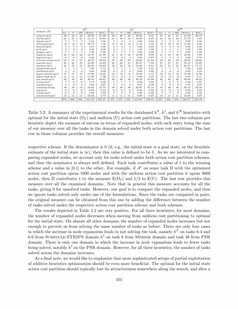
domain (D)hF hI hFI
OI U SB E(OI ) E(U) OI U SB E(OI ) E(U) OI U SB E(OI ) E(U)airport-ipc4 22 22 22 22.00 21.98 22 20 20 20.00 9.55 21 21 21 21.00 20.17blocks-ipc2 21 21 21 14.15 18.84 21 18 18 18.00 2.63 21 18 18 17.79 5.07depots-ipc3 7 7 7 5.14 7.00 7 4 4 4.00 0.91 7 7 7 6.89 5.50driverlog-ipc3 12 12 12 10.77 7.36 13 12 12 11.10 7.32 12 12 12 11.09 6.23freecell-ipc3 5 5 5 3.91 5.00 4 4 4 4.00 2.63 5 4 4 3.90 4.00grid-ipc1 2 2 2 2.00 2.00 2 1 1 1.00 1.00 1 1 1 1.00 1.00gripper-ipc1 7 7 7 7.00 7.00 7 7 7 7.00 6.90 7 7 7 6.96 6.99logistics-ipc2 24 22 22 18.37 21.93 21 16 16 16.00 0.92 21 16 16 16.00 1.69logistics-ipc1 6 6 6 6.00 1.14 5 4 4 4.00 0.87 5 5 5 5.00 0.76miconic-strips-ipc2 53 51 51 48.79 43.04 53 50 50 49.68 31.94 53 50 50 49.05 34.60mprime-ipc1 23 23 23 23.00 12.82 23 22 21 20.91 7.50 21 21 21 19.13 12.60mystery-ipc1 21 21 21 20.90 16.80 18 18 18 18.00 9.81 21 21 21 20.37 17.15openstacks-ipc5 7 7 7 7.00 5.74 7 7 7 7.00 3.21 7 7 7 7.00 4.09pathways-ipc5 4 4 4 4.00 2.36 4 4 4 4.00 4.00 4 4 4 4.00 3.23pipes-notank-ipc4 17 17 17 17.00 12.68 18 15 15 15.00 4.17 16 16 16 16.00 13.30pipes-tank-ipc4 11 11 11 11.00 7.28 11 9 9 9.00 3.27 9 9 9 9.00 5.11psr-small-ipc4 49 49 49 36.35 48.87 48 49 48 38.39 47.90 49 49 49 38.89 48.53rovers-ipc5 7 6 6 5.73 4.06 7 7 7 6.32 5.98 7 6 6 5.48 5.07satellite-ipc4 6 6 6 5.83 2.97 7 6 6 5.67 2.56 7 6 6 5.70 2.67schedule-strips 49 46 44 24.83 31.75 49 40 40 30.87 27.14 47 46 46 38.12 40.33tpp-ipc5 6 6 6 6.00 5.03 6 6 6 6.00 3.56 6 6 6 6.00 4.03trucks-ipc5 6 6 6 5.08 5.89 7 7 7 7.00 6.20 7 7 7 6.82 6.92zenotravel-ipc3 13 11 11 10.34 3.73 11 11 11 9.96 6.97 13 11 11 10.48 5.07
378 368 366 315.18 295.27 371 337 335 312.90 196.94 367 350 350 325.67 254.09
Table 5.2: A summary of the experimental results for the databased hF, hI, and hFI heuristics withoptimal for the initial state (OI) and uniform (U) action cost partitions. The last two columns perheuristic depict the measure of success in terms of expanded nodes, with each entry being the sumof our measure over all the tasks in the domain solved under both action cost partitions. The lastrow in those columns provides the overall measures.
respective scheme. If the denominator is 0 (if, e.g., the initial state is a goal state, or the heuristicestimate of the initial state is ∞), then this value is defined to be 1. As we are interested in com-paring expanded nodes, we account only for tasks solved under both action cost partition schemes,and thus the nominator is always well defined. Each task contributes a value of 1 to the winningscheme and a value in [0,1] to the other. For example, if A∗ on some task Π with the optimizedaction cost partition opens 1000 nodes and with the uniform action cost partition it opens 3000nodes, then Π contributes 1 to the measure E(OI) and 1/3 to E(U). The last row provides thismeasure over all the examined domains. Note that in general this measure accounts for all thetasks, giving 0 for unsolved tasks. However, our goal is to compare the expanded nodes, and thuswe ignore tasks solved only under one of the formulations. Since the tasks are compared in pairs,the original measure can be obtained from this one by adding the difference between the numberof tasks solved under the respective action cost partition scheme and both schemes.
The results depicted in Table 5.2 are very positive. For all three heuristics, for most domains,the number of expanded nodes decreases when moving from uniform cost partitioning to optimalfor the initial state. On almost all other domains, the number of expanded nodes increases but notenough to prevent us from solving the same number of tasks as before. There are only four casesin which the increase in node expansions leads to not solving the task, namely hF on tasks 6-4 and6-6 from Schedule-STRIPS domain hI on task 8 from Mprime domain and task 48 from PSRdomain. There is only one domain in which the increase in node expansions leads to fewer tasksbeing solved, notably hI on the PSR domain. However, for all three heuristics, the number of taskssolved across the domains increases.
As a final note, we would like to emphasize that more sophisticated setups of partial exploitationof additive heuristics optimization should be even more beneficial. The optimal for the initial stateaction cost partition should typically lose its attractiveness somewhere along the search, and after a
101

certain point even the uniform action cost partitioning should be expected to provide more accurateheuristic estimates. Hence, developing meta-reasoning procedures for deciding when (if at all) someeffort should be invested in devising additional action cost partitions is clearly of practical interest.
102
Chapter 6
Summary and Future Work
Our goal in this research was to stratify and extend the machinery of admissible heuristic func-tions for cost-optimal planning. Our contributions towards this goal are in several complimentarydirections. First, we studied the complexity of cost-optimal classical planning with respect to theinterplay between the topology of the problem’s causal graph and certain types of local structuralrestrictions of the problems induced by their action sets. For some problem classes, we have shownthat cost-optimal planning is tractable, and that relaxing the aforementioned restrictions results inNP-hard problem classes. We believe there is room for further extending the palette of tractablecost-optimal planning, and we urge continuing research in this direction.
Exploiting our tractability results for cost-optimal planning, we then introduced a domain-independent framework for devising admissible heuristics using what we call additive implicit ab-stractions. Each such implicit abstraction corresponds to abstracting the planning task at hand byan instance of a tractable fragment of optimal planning. The key motivation for our frameworkwas to escape the restriction of explicit abstractions, such as pattern-database and merge-and-shrink abstractions, to abstract spaces of a fixed size. We presented a concrete scheme for additiveimplicit abstractions by decomposing the planning task along its causal graph and suggested aconcrete realization of this idea, called fork-decomposition, that is based on two novel fragments oftractable cost-optimal planning. We then studied the induced admissible heuristics both formallyand empirically, and showed that they favorably compete in informativeness with the state-of-the-art admissible heuristics both in theory and in practice. Our empirical evaluation stressed thetradeoff between the accuracy of the heuristics and runtime complexity of computing them. To al-leviate the computational overhead of fork-decomposition heuristics, we showed that an equivalentof the explicit abstraction notion of “database” exists also for the fork-decomposition abstractions,despite their exponential-size abstract spaces. Our subsequent empirical evaluation of heuristicsearch with such databases for the fork-decomposition heuristics showed that it favorably competeswith the state of the art of cost-optimal planning.
Another chapter of our work is devoted to additive ensembles of admissible heuristics. Numer-ous recent works have suggested that additive ensembles of admissible heuristics are a powerfultool for heuristic-search systems. However, the action-cost partition parameter of such ensemblesleft the “how to add (if at all)” question completely open. We have developed a procedure thatcloses this question for arbitrary ensembles of all abstraction heuristics with which we are famil-iar, including pattern databases, constrained pattern databases, merge-and-shrink abstractions,fork-decomposition implicit abstractions, and implicit abstractions based on tractable constraint
103
optimization over tree-shaped constraint networks. The procedure is based on a linear-programmingformulation of the optimization problem: given a classical planning task, a forward-search state,and a set of abstraction-based admissible heuristics, the procedure constructs an optimal additivecomposition of these heuristics with respect to the search state in question. Most importantly, thetime complexity of our procedure is polynomial for arbitrary ensembles of all the above abstractionheuristics.
While more informative estimates are naturally appealing, the impractical evaluation time re-quired to solve large-scale linear problems at each search state forced us to seek more pragmaticalternatives. One such alternative is to calculate the optimal cost partitioning not for every statebut only for some (small) subset of states, and use some predefined cost partitioning for the rest 1.We performed an extensive experimental evaluation, calculating the optimal cost partition only inthe initial state. In most cases the informativeness of the heuristic increased, allowing us to solvemore tasks overall.
The basic principles of the implicit abstraction framework motivate further research in numerousdirections, most importantly in
1. discovering new islands of tractability of optimal planning, and
2. abstracting the general planning tasks into such islands.
Likewise, there is promise in combining implicit abstractions with other techniques for deriving ad-missible heuristic estimates. A first step towards combining implicit abstractions with polynomial-time discoverable landmarks of the planning tasks has recently been taken by Domshlak, Katz,and Lefler (2010). We believe that various combinations of such techniques might well improve theinformativeness of the heuristics without substantially increasing their runtime complexity.
Probably the most important entirely open problem is structure optimization. While our frame-work optimizes the composition of a given set of TG-structures, our ultimate goal is to move to evenmore parametric ensembles of this type, allowing flexibility in the actual choice of TG-structures.For instance, it would clearly help to know what PDBs should (optimally) be added to the ensem-ble, what domain abstractions should (optimally) be performed on the roots of the inverted forksand forks, or what polytrees should (optimally) span the causal graph of the task.
When considering additive composition of admissible heuristics, one question that arises almostimmediately is whether a composition based on techniques other than abstraction can be optimizedas well. The current answer to this question is affirmative only in part, and this part turns out to beclosely related to our results here. Karpas and Domshlak (2009) have recently shown that additiveheuristics based on landmarks of the problem’s delete-relaxation (such as hL and hLA of Karpasand Domshlak (2009) and hLM-cut of Helmert and Domshlak (2009)) can be efficiently optimized bysolving a certain compact linear program. That both abstraction and landmark additive heuristicsoptimization procedures are based on linear programming is no coincidence: a recently establishedconnection between such landmark heuristics and the merge-and-shrink abstractions (Helmert &Domshlak, 2009) implies that Karpas and Domshlak’s procedure is effectively a special case of theLP-optimization procedure for the abstractions developed in our work.
In contrast to abstraction and landmark heuristics, the question of additive ensemble optimiza-tion remains open for the hm family of critical path heuristics (Haslum & Geffner, 2000) even for
1Note that the extreme case here would be to give up calculating the optimal cost partitioning altogether forthe sake of speed, using some ad hoc (uniform) cost partition for all states, as we did in the databased implicitabstractions case.
104
the h1 (also known as hmax) member of this family. While computing the additive hm heuristic fora fixed m is poly-time, this computation is not based on an additive abstraction of the planningtask, or, at least, not on a fixed abstraction.2 The state graph over which each hm is computedis an AND/OR-graph (and not an OR-graph, as is the case for transition graphs), and the actualcomputation of hm corresponds to computing a critical tree (and not a shortest path) to the goal.Tangentially, the problem of computing a critical tree in an AND/OR-graph does not appear tohave an LP reformulation. Hence, the complexity of computing the optimal additive hm heuristicis still an open and very interesting question.
Also worth mentioning is that, at first glance, the basic idea of LP-optimizing heuristic com-position naturally extends also to intractable planning relaxations that admit “second-order” LP-relaxations. For instance, some intractable planning relaxations formalizable via integer-valued LPs(such as the deletes-ignoring relaxation underlying h+, or the more recent action-ordering relaxationof van den Briel, Benton, Kambhampati, & Vossen, 2007) appear to be quite natural candidates.Things, however, are more complicated than that because, in short, Definition 19 (p. 84) requires avery specific type of LP-encoding. Encodings of this type must satisfy Eq. 5.4 (p. 84), but we knowof no ILP-to-LP ”second-order” relaxations that meet this requirement. Thus, the most interestingquestion of incorporating such relaxations still remains open.
Finally, considering the empirical promise of optimal action cost partitioning, we note thatthe linear programs induced by our LP-encoding technique have a specific structure called in theliterature primal block-angular (Castro, 2007). This structure can possibly be exploited for devisinga more efficient algorithm for optimal action cost partitioning, and this is an interesting venue forfuture research. Tangentially, the development of automated procedures for devising fixed-sizeportfolios of action cost partitions is a promising direction, as all the states examined during thesearch might be “well served” by these procedures.
We believe that pursuing research in all these directions may substantially increase the infor-mativeness and runtime efficiency of implicit abstraction heuristics both per se and in the scope ofadditive ensembles of admissible heuristics.
2To the best of our knowledge, the precise relation between critical path and abstraction heuristics is currentlyan open question, the only exception being additive h1, now known to be closely related to the landmark heuris-tics (Helmert & Domshlak, 2009).
105

106
Bibliography
Allen, J., Hendler, J., & Tate, A. (Eds.). (1990). Readings in Planning. Morgan-Kaufmann.
Bacchus, F., & Yang, Q. (1994). Downward refinement and the efficiency of hierarchical problemsolving. Artificial Intelligence, 71 (1), 43–100.
Backstrom, C., & Klein, I. (1991). Planning in polynomial time: The SAS-PUBS class. Computa-tional Intelligence, 7 (3), 181–197.
Backstrom, C., & Nebel, B. (1995). Complexity results for SAS+ planning. Computational Intelli-gence, 11 (4), 625–655.
Ball, M., & Holte, R. C. (2008). The compression power of symbolic pattern databases. In Proceed-ings of the 18th International Conference on Automated Planning and Scheduling (ICAPS),pp. 2–11, Sydney, Australia.
Bonet, B., & Geffner, H. (2001). Planning as heuristic search. Artificial Intelligence, 129 (1–2),5–33.
Bonet, B., & Geffner, H. (2006). Heuristics for planning with penalties and rewards using com-piled knowledge. In Proceedings of the International Conference on Principles of KnowledgeRepresentation and Reasoning (KR), pp. 452–462.
Boutilier, C., Brafman, R., Domshlak, C., Hoos, H., & Poole, D. (2004). CP-nets: A tool forrepresenting and reasoning about conditional ceteris paribus preference statements. Journalof Artificial Intelligence Research, 21, 135–191.
Brafman, R. I., & Domshlak, C. (2003). Structure and complexity of planning with unary operators.Journal of Artificial Intelligence Research, 18, 315–349.
Bylander, T. (1994). The computational complexity of propositional STRIPS planning. ArtificialIntelligence, 69 (1-2), 165–204.
Castro, J. (2007). An interior-point approach for primal block-angular problems. ComputationalOptimization and Applications, 36 (2-3), 195–219.
Chapman, D. (1987). Planning for conjunctive goals. Artificial Intelligence, 32 (3), 333–377.
Chen, H., & Gimenez, O. (2008). Causal graphs and structurally restricted planning. In Proceedingsof the 18th International Conference on Automated Planning and Scheduling (ICAPS), pp.36–43, Sydney, Australia.
Clarke, E., Grumberg, O., & Peled, D. (1999). Model Checking. MIT Press.
Coles, A. I., Fox, M., Long, D., & Smith, A. J. (2008). Additive-disjunctive heuristics for optimalplanning. In Proceedings of the 18th International Conference on Automated Planning andScheduling (ICAPS), pp. 44–51.
107
Cormen, T. H., Leiserson, C. E., & Rivest, R. L. (1990). Introduction to Algorithms. MIT Press.
Culberson, J., & Schaeffer, J. (1998). Pattern databases. Computational Intelligence, 14 (4), 318–334.
Dean, T., & Wellman, M. (1991). Planning and Control. Morgan-Kaufmann.
Dechter, R. (2003). Constraint Processing. Morgan Kaufmann.
Dechter, R., & Pearl, J. (1985). Generalized best-first search strategies and the optimality of a*.J. ACM, 32 (3), 505–536.
Domshlak, C., & Dinitz, Y. (2001). Multi-agent off-line coordination: Structure and complexity. InProceedings of Sixth European Conference on Planning (ECP), pp. 277–288.
Domshlak, C., & Hoffmann, J. (2006). Fast probabilistic planning through weighted model counting.In Proceedings of the 16th International Conference on Automated Planning and Scheduling(ICAPS), pp. 243–252.
Domshlak, C., Hoffmann, J., & Sabharwal, A. (2009). Friends or foes? On planning as satisfiabilityand abstract CNF encodings. Journal of Artificial Intelligence Research, 36, 415–469.
Domshlak, C., Katz, M., & Lefler, S. (2010). When abstractions met landmarks. In Proceedingsof the 20th International Conference on Automated Planning and Scheduling (ICAPS), pp.50–56, Toronto, Canada.
Drager, K., Finkbeiner, B., & Podelski, A. (2006). Directed model checking with distance-preservingabstractions. In Valmari, A. (Ed.), Proceedings of the 13th International SPIN Workshop onModel Checking Software, Vol. 3925 of Lecture Notes in Computer Science, pp. 19–36, BerlinHeidelberg. Springer-Verlag.
Edelkamp, S. (2001). Planning with pattern databases. In Proceedings of the European Conferenceon Planning (ECP), pp. 13–34.
Edelkamp, S. (2002). Symbolic pattern databases in heuristic search planning. In Proceedings ofthe International Conference on AI Planning and Scheduling (AIPS), pp. 274–293.
Edelkamp, S. (2006). Automated creation of pattern database search heuristics. In Proceedings ofthe 4th Workshop on Model Checking and Artificial Intelligence (MoChArt).
Edelkamp, S., & Kissmann, P. (2009). Optimal symbolic planning with action costs and preferences.In Proceedings of the 21st International Joint Conference on Artificial Intelligence (IJCAI),pp. 1690–1695, Pasadena, CA, US.
Erol, K., Nau, D. S., & Subrahmanian, V. S. (1995). Complexity, decidability and undecidabilityresults for domain-independent planning. Artificial Intelligence, Special Issue on Planning,76 (1–2), 75–88.
Felner, A., Korf, R. E., & Hanan, S. (2004). Additive pattern database heuristics. Journal ofArtificial Intelligence Research, 22, 279–318.
Fikes, R. E., & Nilsson, N. (1971). STRIPS: A new approach to the application of theorem provingto problem solving. AI Magazine, 2, 189–208.
Garey, M. R., & Johnson, D. S. (1978). Computers and Intractability: A Guide to the Theory ofNP-Completeness. W.H. Freeman and Company, New-York.
108
Geffner, H. (2002). Perspectives on artificial intelligence planning. In Proceedings of the EighteenthNational Conference on Artificial intelligence (AAAI), pp. 1013–1023.
Gerevini, A., Saetti, A., & Serina, I. (2003). Planning through stochastic local search and temporalaction graphs. Journal of Artificial Intelligence Research, 20, 239–290.
Ghallab, M., Nau, D., & Traverso, P. (2004). Automated Planning. Morgan Kaufmann.
Hart, P. E., Nilsson, N. J., & Raphael, B. (1968). A formal basis for the heuristic determination ofminimum cost paths. Systems Science and Cybernetics, IEEE Transactions on, 4 (2), 100–107.
Haslum, P. (2006). Admissible Heuristics for Automated Planning. Ph.D. thesis, Linkoping Uni-versity, Department of Computer and Information Science.
Haslum, P. (2008). Additive and reversed relaxed reachability heuristics revisited. In Proceedingsof the 6th International Planning Competition.
Haslum, P., Bonet, B., & Geffner, H. (2005). New admissible heuristics for domain-independentplanning. In Proceedings of the Twentieth National Conference on Artificial Intelligence(AAAI), pp. 1163–1168.
Haslum, P., Botea, A., Helmert, M., Bonet, B., & Koenig, S. (2007). Domain-independent con-struction of pattern database heuristics for cost-optimal planning. In Proceedings of the 19thNational Conference on Artificial Intelligence (AAAI), pp. 1007–1012.
Haslum, P., & Geffner, H. (2000). Admissible heuristics for optimal planning. In Proceedings ofthe Fifth International Conference on Artificial Intelligence Planning Systems (ICAPS), pp.140–149.
Helmert, M. (2003). Complexity results for standard benchmark domains in planning. ArtificialIntelligence, 146 (2), 219–262.
Helmert, M. (2004). A planning heuristic based on causal graph analysis. In Proceedings of the14th International Conference on Automated Planning and Scheduling (ICAPS), pp. 161–170,Whistler, Canada.
Helmert, M. (2006). The Fast Downward planning system. Journal of Artificial Intelligence Re-search, 26, 191–246.
Helmert, M., & Domshlak, C. (2009). Landmarks, critical paths and abstractions: What’s the dif-ference anyway?. In Proceedings of the 19th International Conference on Automated Planningand Scheduling (ICAPS), pp. 162–169, Thessaloniki, Greece.
Helmert, M., Haslum, P., & Hoffmann, J. (2007). Flexible abstraction heuristics for optimal sequen-tial planning. In Proceedings of the 17th International Conference on Automated Planningand Scheduling (ICAPS), pp. 176–183, Providence, RI, USA.
Helmert, M., & Mattmuller, R. (2008). Accuracy of admissible heuristic functions in selectedplanning domains. In Proceedings of the 23rd AAAI Conference on Artificial Intelligence, pp.938–943, Chicago, USA.
Helmert, M. (2008). Understanding Planning Tasks: Domain Complexity and Heuristic Decompo-sition, Vol. 4929 of Lecture Notes in Computer Science. Springer.
Hendler, J., Tate, A., & Drummond, M. (1990). Ai planning: systems and techniques. AI Magazine,11 (2), 61–77.
109
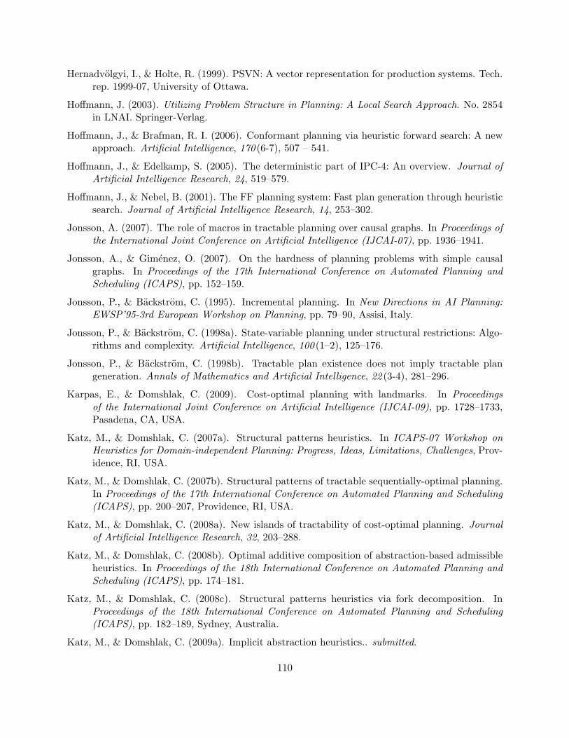
Hernadvolgyi, I., & Holte, R. (1999). PSVN: A vector representation for production systems. Tech.rep. 1999-07, University of Ottawa.
Hoffmann, J. (2003). Utilizing Problem Structure in Planning: A Local Search Approach. No. 2854in LNAI. Springer-Verlag.
Hoffmann, J., & Brafman, R. I. (2006). Conformant planning via heuristic forward search: A newapproach. Artificial Intelligence, 170 (6-7), 507 – 541.
Hoffmann, J., & Edelkamp, S. (2005). The deterministic part of IPC-4: An overview. Journal ofArtificial Intelligence Research, 24, 519–579.
Hoffmann, J., & Nebel, B. (2001). The FF planning system: Fast plan generation through heuristicsearch. Journal of Artificial Intelligence Research, 14, 253–302.
Jonsson, A. (2007). The role of macros in tractable planning over causal graphs. In Proceedings ofthe International Joint Conference on Artificial Intelligence (IJCAI-07), pp. 1936–1941.
Jonsson, A., & Gimenez, O. (2007). On the hardness of planning problems with simple causalgraphs. In Proceedings of the 17th International Conference on Automated Planning andScheduling (ICAPS), pp. 152–159.
Jonsson, P., & Backstrom, C. (1995). Incremental planning. In New Directions in AI Planning:EWSP’95-3rd European Workshop on Planning, pp. 79–90, Assisi, Italy.
Jonsson, P., & Backstrom, C. (1998a). State-variable planning under structural restrictions: Algo-rithms and complexity. Artificial Intelligence, 100 (1–2), 125–176.
Jonsson, P., & Backstrom, C. (1998b). Tractable plan existence does not imply tractable plangeneration. Annals of Mathematics and Artificial Intelligence, 22 (3-4), 281–296.
Karpas, E., & Domshlak, C. (2009). Cost-optimal planning with landmarks. In Proceedingsof the International Joint Conference on Artificial Intelligence (IJCAI-09), pp. 1728–1733,Pasadena, CA, USA.
Katz, M., & Domshlak, C. (2007a). Structural patterns heuristics. In ICAPS-07 Workshop onHeuristics for Domain-independent Planning: Progress, Ideas, Limitations, Challenges, Prov-idence, RI, USA.
Katz, M., & Domshlak, C. (2007b). Structural patterns of tractable sequentially-optimal planning.In Proceedings of the 17th International Conference on Automated Planning and Scheduling(ICAPS), pp. 200–207, Providence, RI, USA.
Katz, M., & Domshlak, C. (2008a). New islands of tractability of cost-optimal planning. Journalof Artificial Intelligence Research, 32, 203–288.
Katz, M., & Domshlak, C. (2008b). Optimal additive composition of abstraction-based admissibleheuristics. In Proceedings of the 18th International Conference on Automated Planning andScheduling (ICAPS), pp. 174–181.
Katz, M., & Domshlak, C. (2008c). Structural patterns heuristics via fork decomposition. InProceedings of the 18th International Conference on Automated Planning and Scheduling(ICAPS), pp. 182–189, Sydney, Australia.
Katz, M., & Domshlak, C. (2009a). Implicit abstraction heuristics.. submitted.
110
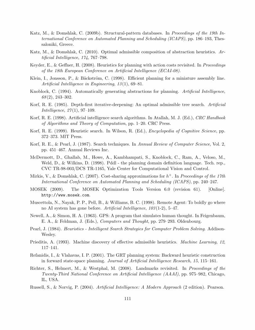
Katz, M., & Domshlak, C. (2009b). Structural-pattern databases. In Proceedings of the 19th In-ternational Conference on Automated Planning and Scheduling (ICAPS), pp. 186–193, Thes-saloniki, Greece.
Katz, M., & Domshlak, C. (2010). Optimal admissible composition of abstraction heuristics. Ar-tificial Intelligence, 174, 767–798.
Keyder, E., & Geffner, H. (2008). Heuristics for planning with action costs revisited. In Proceedingsof the 18th European Conference on Artificial Intelligence (ECAI-08).
Klein, I., Jonsson, P., & Backstrom, C. (1998). Efficient planning for a miniature assembly line.Artificial Intelligence in Engineering, 13 (1), 69–81.
Knoblock, C. (1994). Automatically generating abstractions for planning. Artificial Intelligence,68 (2), 243–302.
Korf, R. E. (1985). Depth-first iterative-deepening: An optimal admissible tree search. ArtificialIntelligence, 27 (1), 97–109.
Korf, R. E. (1998). Artificial intelligence search algorithms. In Atallah, M. J. (Ed.), CRC Handbookof Algorithms and Theory of Computation, pp. 1–20. CRC Press.
Korf, R. E. (1999). Heuristic search. In Wilson, R. (Ed.), Encyclopedia of Cognitive Science, pp.372–373. MIT Press.
Korf, R. E., & Pearl, J. (1987). Search techniques. In Annual Review of Computer Science, Vol. 2,pp. 451–467. Annual Reviews Inc.
McDermott, D., Ghallab, M., Howe, A., Kambhampati, S., Knoblock, C., Ram, A., Veloso, M.,Weld, D., & Wilkins, D. (1998). Pddl - the planning domain definition language. Tech. rep.,CVC TR-98-003/DCS TR-1165, Yale Center for Computational Vision and Control.
Mirkis, V., & Domshlak, C. (2007). Cost-sharing approximations for h+. In Proceedings of the 17thInternational Conference on Automated Planning and Scheduling (ICAPS), pp. 240–247.
MOSEK (2009). The MOSEK Optimization Tools Version 6.0 (revision 61). [Online].http://www.mosek.com.
Muscettola, N., Nayak, P. P., Pell, B., & Williams, B. C. (1998). Remote Agent: To boldly go whereno AI system has gone before. Artificial Intelligence, 103 (1-2), 5–47.
Newell, A., & Simon, H. A. (1963). GPS: A program that simulates human thought. In Feigenbaum,E. A., & Feldman, J. (Eds.), Computers and Thought, pp. 279–293. Oldenbourg.
Pearl, J. (1984). Heuristics - Intelligent Search Strategies for Computer Problem Solving. Addison-Wesley.
Prieditis, A. (1993). Machine discovery of effective admissible heuristics. Machine Learning, 12,117–141.
Refanidis, I., & Vlahavas, I. P. (2001). The GRT planning system: Backward heuristic constructionin forward state-space planning. Journal of Artificial Intelligence Research, 15, 115–161.
Richter, S., Helmert, M., & Westphal, M. (2008). Landmarks revisited. In Proceedings of theTwenty-Third National Conference on Artificial Intelligence (AAAI), pp. 975–982, Chicago,IL, USA.
Russell, S., & Norvig, P. (2004). Artificial Intelligence: A Modern Approach (2 edition). Pearson.
111
Sacerdoti, E. (1974). Planning in a hierarchy of abstraction spaces. Artificial Intelligence, 5,115–135.
Schrijver, A. (1998). Theory of Linear and Integer Programming. John Wiley & Sons.
Tenenberg, J. D. (1991). Abstraction in planning. In Allen, J. F., Kautz, H. A., Pelavin, R. N., &Tenenberg, J. D. (Eds.), Reasoning About Plans, chap. 4, pp. 213–284. Morgan Kaufmann.
van den Briel, M., Benton, J., Kambhampati, S., & Vossen, T. (2007). An LP-based heuristicfor optimal planning. In Proceedings of the 13th International Conference on Principles andPractice of Constraint Programming (CP), pp. 651–665, Providence, RI, USA.
Vidal, V. (2004). A lookahead strategy for heuristic search planning. In Proceedings of the 14thInternational Conference on Automated Planning and Scheduling (ICAPS), pp. 150–160.
Weld, D. S. (1999). Recent advances in AI planning. AI Magazine, 20 (2), 93–123.
Wilkins, D. E. (1984). Domain-independent planning: Representation and plan generation. ArtificialIntelligence, 22, 269–301.
Williams, B., & Nayak, P. (1996). A model-based approach to reactive self-configuring systems.In Proceedings of the Thirteenth National Conference on Artificial Intelligence, pp. 971–977,Portland, OR. AAAI Press.
Williams, B., & Nayak, P. (1997). A reactive planner for a model-based executive. In Proceedingsof the 15th International Joint Conference on Artificial Intelligence (IJCAI), pp. 1178–1185,Nagoya, Japan.
Yang, F., Culberson, J., & Holte, R. (2007). A general additive search abstraction. Tech. rep.TR07-06, University of Alberta.
Yang, F., Culberson, J., Holte, R., Zahavi, U., & Felner, A. (2008). A general theory of additivestate space abstractions. Journal of Artificial Intelligence Research, 32, 631–662.
Zhou, R., & Hansen, E. (2006). Breadth-first heuristic search. Artificial Intelligence, 170, 385–408.
112
Appendix A
Compexity Results in Detail
A.1 Cost-Optimal Planning for Pb
This section is devoted to the proof of tractability of cost-optimal planning for the problem fragmentPb. We begin with describing our planning-to-COP scheme for Pb, and then prove its correctnessand complexity.
A.1.1 Construction
Before we proceed with the details of the construction, here we make an assumption that thespecification of our actions is fully specified in terms of the variable parents in the causal graph.If pred(v) ⊂ V denotes the set of all the immediate predecessors of v in the causal graph CG(Π),then we assume that, for each action a ∈ Av, pre(a)[w] is specified for each w ∈ pred(v). While ingeneral such an assumption requires an exponential translation, this is not the case with Pb. LetA./ be such a translation of the original problem actions A. To obtain A./, for every variable v ∈ V ,every action in Av is represented in A./ by a set of actions that are preconditioned by completeassignments to pred(v). If |pred(v)| = k, and the precondition of a is specified only in terms ofsome 0 ≤ k′ ≤ k parents of v, then a is represented in A./ by a set of actions, each extendingthe precondition pre(a) by a certain instantiation of the previously unspecified k − k′ parents ofv, and having the cost cost./(a′) = cost(a). Note that the expansions of two or more originalactions may overlap, and thus A./ may contain syntactically identical yet differently priced actions.Without loss of generality, we assume that only a minimally-priced such clone is kept in A./. Thekey point is that that compiling A into A./ for the Pb problems is poly-time, as the procedure islinear in |A./| = O(n2In(Π)+1). Finally, the (straightforward to prove) Proposition 1 summarizesthe correctness of our assumption with respect to the cost-optimal planning for ub.
Proposition 1 For any ub task Π = 〈V ,A, I ,G, cost〉, the cost of the optimal plans for Π is equalto this for Π./ = 〈V,A./, I, G, cost./〉, with optimal plans for Π being reconstructible in linear timefrom the optimal plans for Π./ and vice versa.
We now specify our compilation of a given Pb task Π into a constraint optimization problemCOPΠ. The COP variable set X contains a variable xv for each planning variable v ∈ V , and the
113
domain D(xv) consists of all valid prefixes of τ(v). That is,
X = {xv | v ∈ V }D(xv) = �∗[τ(v)]
(A.1)
Informally, the domain of each variable xv contains all possible sequences of values that the planningvariable v may undergo along a cost-optimal plan. Now, for each planning variable v with parentspred(v) = {w1, . . . , wk}, the set of COP functions F contains a single non-negative, real-valuedfunction ϕv with the scope
Qv = {xv, xw1 , . . . , xwk} (A.2)
The purpose of these functions is to connect between the value-changing sequences of v and these ofits parents pred(v). The specification of these functions is the more involved part of the compilation.
First, for each planning variable v with pred(v) = ∅, and each of its goal-valid (time-stamped)value-changing sequences τ ′ ∈ �∗[τ(v)], we set
ϕv(τ ′) =⌊ |τ ′|
2
⌋· C(awv) +
⌊ |τ ′| − 12
⌋· C(abv) (A.3)
where eff(awv)[v] = {wv}, eff(abv)[v] = bv, and C(a) = cost(a) if a ∈ A, and ∞, otherwise. It isnot hard to verify that ϕv(τ ′) corresponds to the optimal cost of performing |σ′| − 1 value changesof v in Π.
Now, for each non-root variable v with pred(v) = {w1, . . . , wk}, k ≥ 1, we specify the functionϕv as follows. For each goal-valid value-changing sequence τ ′ ∈ �∗[τ(v)] of v, and each set ofsuch goal-valid value-changing sequences {τ ′1 ∈ �∗[τ(w1)], . . . , τ ′k ∈ �∗[τ(wk)]} of v’s parents, wewant to set ϕv(τ ′, τ ′1, . . . , τ
′k) to the optimal cost of performing |τ ′| − 1 value changes of v, given
that w1, . . . , wk change their values |τ ′1| − 1, . . . , |τ ′k| − 1 times, respectively. In what follows, wereduce setting the value ϕv(τ ′, τ ′1, . . . , τ
′k) to solving a single-source shortest path problem on an
edge-weighted digraph G′e(v) that slightly enhances a similarly-named graphical structure suggestedby Brafman and Domshlak (2003). Though the construction of G′e(v) is very similar to this of Braf-man and Domshlak (2003), here we provide it in full details to save the reader patching the essentialdifferences from the construction of Brafman and Domshlak (2003).
Given the value-changing sequences τ ′1, . . . , τ′k as above, the digraph G′e(v) is created in three
steps. First, we construct a labeled directed graph G(v) capturing information about all sequencesof assignments on pred(v) that can enable n or less value flips of v. The graph G(v) is defined asfollows:
1. G(v) consist of η = maxτ ′∈�∗[τ(v)] |τ ′| nodes.
2. G(v) forms a 2-colored multichain, i.e., (i) the nodes of the graph are colored with black (b)and white (w), starting with black; (ii) there are no two subsequent nodes with the samecolor; (iii) for 1 ≤ i ≤ η − 1, edges from the node i are only to the node i+ 1.
Observe that such a construction of G(v) promises that the color of the last node will beconsistent with the goal value G[v] if such is specified.
3. The nodes of G(v) are denoted precisely by the elements of the longest goal-valid value-changing sequence τ ′ ∈ �∗[τ(v)], that is, biv stands for the ith black node in G(v).
114
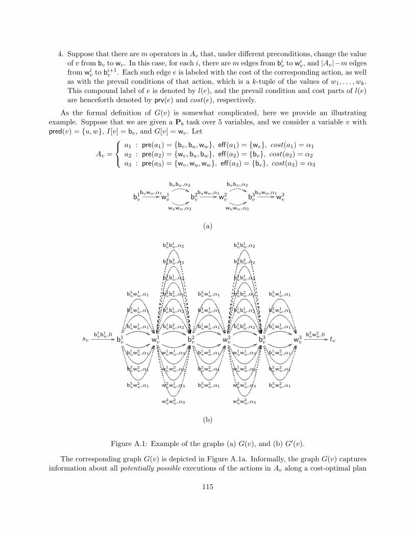
4. Suppose that there are m operators in Av that, under different preconditions, change the valueof v from bv to wv. In this case, for each i, there are m edges from biv to wi
v, and |Av|−m edgesfrom wi
v to bi+1v . Each such edge e is labeled with the cost of the corresponding action, as well
as with the prevail conditions of that action, which is a k-tuple of the values of w1, . . . , wk.This compound label of e is denoted by l(e), and the prevail condition and cost parts of l(e)are henceforth denoted by prv(e) and cost(e), respectively.
As the formal definition of G(v) is somewhat complicated, here we provide an illustratingexample. Suppose that we are given a Pb task over 5 variables, and we consider a variable v withpred(v) = {u,w}, I[v] = bv, and G[v] = wv. Let
Av =
a1 : pre(a1) = {bv, bu,ww}, eff(a1) = {wv}, cost(a1) = α1
a2 : pre(a2) = {wv, bu, bw}, eff(a2) = {bv}, cost(a2) = α2
a3 : pre(a3) = {wv,wu,ww}, eff(a3) = {bv}, cost(a3) = α3
b1v
buww,α1// w1v
bubw,α2
$$
wuww,α3
:: b2v
buww,α1// w2v
bubw,α2
$$
wuww,α3
:: b3v
buww,α1// w3v
(a)
svb1ub1w,0 // b1
v
b1uw1
w,α1
&&
b1uw2
w,α1
88
b2uw1
w,α1
��
b2uw2
w,α1
HH
b3uw1
w,α1
��
b3uw2
w,α1
KKw1v
b1ub1w,α2
��b1ub2w,α2
%%
b2ub1w,α2
��
b2ub2w,α2
��
b3ub1w,α2
��
b3ub2w,α2
��
w1uw1
w,α3
99
w1uw2
w,α3
HH
w2uw1
w,α3
KK
w2uw2
w,α3
LLb2v
b1uw1
w,α1
&&
b1uw2
w,α1
88
b2uw1
w,α1
��
b2uw2
w,α1
HH
b3uw1
w,α1
��
b3uw2
w,α1
KKw2v
b1ub1w,α2
��b1ub2w,α2
%%
b2ub1w,α2
��
b2ub2w,α2
��
b3ub1w,α2
��
b3ub2w,α2
��
w1uw1
w,α3
99
w1uw2
w,α3
HH
w2uw1
w,α3
KK
w2uw2
w,α3
LLb3v
b1uw1
w,α1
&&
b1uw2
w,α1
88
b2uw1
w,α1
��
b2uw2
w,α1
HH
b3uw1
w,α1
��
b3uw2
w,α1
KKw3v
b3uw2
w,0 // tv
(b)
Figure A.1: Example of the graphs (a) G(v), and (b) G′(v).
The corresponding graph G(v) is depicted in Figure A.1a. Informally, the graph G(v) capturesinformation about all potentially possible executions of the actions in Av along a cost-optimal plan
115
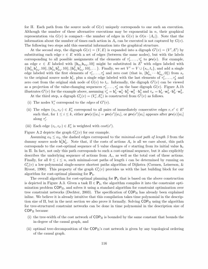
for Π. Each path from the source node of G(v) uniquely corresponds to one such an execution.Although the number of these alternative executions may be exponential in n, their graphicalrepresentation via G(v) is compact—the number of edges in G(v) is O(n · |Av|). Note that theinformation about the number of times each action in Av can be executed is not captured by G(v).The following two steps add this essential information into the graphical structure.
At the second step, the digraph G(v) = (V,E) is expanded into a digraph G′(v) = (V ′, E′) bysubstituting each edge e ∈ E with a set of edges (between the same nodes), but with the labelscorresponding to all possible assignments of the elements of τ ′1, . . . , τ
′k to prv(e). For example,
an edge e ∈ E labeled with ‖bw1bw2 , 10‖ might be substituted in E′ with edges labeled with{‖b1
w1b1w2, 10‖, ‖b1
w1b2w2, 10‖, ‖b2
w1b1w2, 10‖, . . . }. Finally, we set V ′ = V ∪ {sv, tv}, and add a single
edge labeled with the first elements of τ ′1, . . . , τ′k and zero cost (that is, ‖b1
w1· · · b1
wk, 0‖) from sv
to the original source node b1v, plus a single edge labeled with the last elements of τ ′1, . . . , τ
′k and
zero cost from the original sink node of G(v) to tv. Informally, the digraph G′(v) can be viewedas a projection of the value-changing sequences τ ′1, . . . , τ
′k on the base digraph G(v). Figure A.1b
illustrates G′(v) for the example above, assuming τ ′u = b1u ·w1
u ·b2u ·w2
u ·b3u and τw = b1
w ·w1w ·b2
w ·w2w.
At the third step, a digraph G′e(v) = (V ′e , E′e) is constructed from G′(v) as follows.
(i) The nodes V ′e correspond to the edges of G′(v).
(ii) The edges (ve, ve′) ∈ E′e correspond to all pairs of immediately consecutive edges e, e′ ∈ E′such that, for 1 ≤ i ≤ k, either prv(e)[wi] = prv(e′)[wi], or prv(e′)[wi] appears after prv(e)[wi]along τ ′i .
(iii) Each edge (ve, ve′) ∈ E′e is weighted with cost(e′).
Figure A.2 depicts the graph G′e(v) for our example.Assuming α3 ≤ α2, the dashed edges correspond to the minimal-cost path of length 5 from the
dummy source node b1ub1w. Note that, if the costs of actions Av is all we care about, this path
corresponds to the cost-optimal sequence of 5 value changes of v starting from its initial value bvin Π. In fact, not only this path corresponds to such a cost-optimal sequence, but it also explicitlydescribes the underlying sequence of actions from Av, as well as the total cost of these actions.Finally, for all 0 ≤ i ≤ n, such minimal-cost paths of length i can be determined by running onG′e(v) a low-polynomial single-source shortest paths algorithm of Dijkstra (Cormen, Leiserson, &Rivest, 1990). This property of the graph G′e(v) provides us with the last building block for ouralgorithm for cost-optimal planning for Pb.
The overall algorithm for cost-optimal planning for Pb that is based on the above constructionis depicted in Figure A.3. Given a task Π ∈ Pb, the algorithm compiles it into the constraint opti-mization problem COPΠ, and solves it using a standard algorithm for constraint optimization overtree constraint networks (Dechter, 2003). The specification of COPΠ has already been explainedinline. We believe it is already intuitive that this compilation takes time polynomial in the descrip-tion size of Π, but in the next section we also prove it formally. Solving COPΠ using the algorithmfor tree-structured constraint networks can be done in time polynomial in the description size ofCOPΠ because
(i) the tree-width of the cost network of COPΠ is bounded by the same constant that bounds thein-degree of the causal graph, and
(ii) optimal tree-decomposition of the COPΠ’s cost network is given by any topological orderingof the causal graph.
116
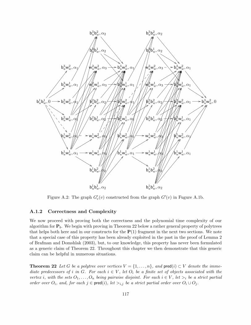
b3ub2w, α2
��99999999999999999b3ub2w, α2
��99999999999999999
b3ub1w, α2
%%LLLLLLLLLL
��99999999999999999b3ub1w, α2
%%LLLLLLLLLL
��99999999999999999
b3uw2
w, α1 w2uw2
w, α3// b3uw2
w, α1 w2uw2
w, α3//__ b3uw2
w, α1
��88888888888888888
b3uw1
w, α1
FF w2uw1
w, α3
99rrrrrrrrrr// b3uw1
w, α1
FF w2uw1
w, α3
99rrrrrrrrrr// b3uw1
w, α1
%%JJJJJJJJJ
b1ub1w, 0
CC�����������������
99ttttttttt//
%%JJJJJJJJJ
��77
77
77
77
7
��/////////////////////////b2uw2
w, α1
BB�����������������b2ub2w, α2
BB�����������������// b2uw2
w, α1
BB��
��
��
��
�b2ub2w, α2
BB�����������������// b2uw2
w, α1// b3uw2
w, 0
b2uw1
w, α1
99rrrrrrrrrr
BB�����������������
FF
JJ�����������������������������������������b2ub1w, α2
FF
BB�����������������
99rrrrrrrrrr// b2uw1
w, α1
99rrrrrrrrrr
BB�����������������
FF
JJ�����������������������������������������b2ub1w, α2
FF
BB�����������������
99rrrrrrrrrr// b2uw1
w, α1
99ttttttttt
b1uw2
w, α1//__
HH���������������������������������w1uw2
w, α3
HH���������������������������������
BB��
��
��
��
�b1uw2
w, α1//
HH���������������������������������w1uw2
w, α3
HH���������������������������������
BB�����������������b1uw2
w, α1
CC�����������������
b1uw1
w, α1
%%LLLLLLLLLL//
99rrrrrrrrrr
FF
HH���������������������������������
JJ�����������������������������������������
KK���������������������������������������������������������w1uw1
w, α3
JJ�����������������������������������������
HH���������������������������������
FF
BB�����������������b1uw1
w, α1
%%LLLLLLLLLL//
99rrrrrrrrrr
FF
HH���������������������������������
JJ�����������������������������������������
KK���������������������������������������������������������w1uw1
w, α3
JJ�����������������������������������������
HH���������������������������������
FF
BB�����������������b1uw1
w, α1
GG�������������������������
b1ub2w, α2
KK�������������������������������������������������
HH���������������������������������
BB�����������������b1ub2w, α2
KK�������������������������������������������������
HH���������������������������������
BB�����������������
b1ub1w, α2
KK���������������������������������������������������������
KK�������������������������������������������������
JJ�����������������������������������������
HH���������������������������������
FF
BB�����������������b1ub1w, α2
KK���������������������������������������������������������
KK�������������������������������������������������
JJ�����������������������������������������
HH���������������������������������
FF
BB�����������������
Figure A.2: The graph G′e(v) constructed from the graph G′(v) in Fugure A.1b.
A.1.2 Correctness and Complexity
We now proceed with proving both the correctness and the polynomial time complexity of ouralgorithm for Pb. We begin with proving in Theorem 22 below a rather general property of polytreesthat helps both here and in our constructs for the P(1) fragment in the next two sections. We notethat a special case of this property has been already exploited in the past in the proof of Lemma 2of Brafman and Domshlak (2003), but, to our knowledge, this property has never been formulatedas a generic claim of Theorem 22. Throughout this chapter we then demonstrate that this genericclaim can be helpful in numerous situations.
Theorem 22 Let G be a polytree over vertices V = {1, . . . , n}, and pred(i) ⊂ V denote the imme-diate predecessors of i in G. For each i ∈ V , let Oi be a finite set of objects associated with thevertex i, with the sets O1, . . . , On being pairwise disjoint. For each i ∈ V , let >i be a strict partialorder over Oi, and, for each j ∈ pred(i), let >i,j be a strict partial order over Oi ∪Oj.
117
If, for each i ∈ V, j ∈ pred(i), the transitively closed >i ∪ >i,j and >j ∪ >i,j induce (strict)partial orders over Oi ∪Oj, then so does the transitively closed
> =⋃i∈V
>i ∪ ⋃j∈pred(i)
>i,j
over O =
⋃i∈V Oi.
Proof: In what follows, by oi we denote an arbitrary object from Oi. Assume to the contrary thatboth >i ∪ >i,j and >j ∪ >i,j are (strict) partial orders, and yet > is not so. That is, there existsa pair of objects oi, oj ∈ O for which hold both oi > oj and oj > oi. By the construction of >,we have that there is a, possibly empty, path between the vertices i and j in the undirected graphinduced by G. Since G is a polytree, we know that such an undirected path between i and j isunique. Thus, we must have
α : oi = o1i0 < . . . < ox0
i0< o1
i1 < . . . < ox1i1< . . . . . . < o1
im < . . . < oxmim = oj
β : oi = o1i0 > . . . > oy0
i0> o1
i1 > . . . > oy1i1> . . . . . . > o1
im > . . . > oymim = oj(A.4)
such that, for 0 ≤ k ≤ m, both xk ≥ 1 and yk ≥ 1, and each step in both chains α and β is directlyimplied by some “local” relation >l or >l,l′ constructing >. The corresponding unique undirectedpath between i and j is:
i = i0 · i1 · . . . · im−1 · im = j (A.5)
Without loss of generality, we assume that the cycle in > induced by α and β is length-wise minimalamong all such cycles in >. In particular, this implies that
(i) for 0 ≤ k ≤ m, we have 1 ≤ xk, yk ≤ 2,
(ii) for each pair of objects o ∈ α, o′ ∈ β, we have o 6= o′, unless o = o′ = oi or o = o′ = oj , and
(iii) for each pair of objects o ∈ α, o′ ∈ β, no >l (and no >l,l′) implies o′ �l o (respectively,o′ �l,l′ o).
First, let us show that at least one of the chains α and β contains at least one internal element.Assume, to the contrary, that both α and β contain no internal elements. If i = j, then we haveoi >i o
′i (where o′i = oj) and o′i >i oi, contradicting our assumption that >i is a partial order. (If
>i is not a partial order, then so is each >i ∪ >i,j .) Otherwise, if i 6= j, then either i ∈ pred(j) orj ∈ pred(i). Assuming the latter, (oi > oj)∧(oi > oj) implies (oi >i,j oj)∧(oi >i,j oj), contradictingour assumption that >i,j is a partial order.
Given that, let us now prove that oxmim 6= oymim , contradicting the assumption that the chains αand β as in Eq. A.4 exist. We do it on a case-by-case basis of possible combinations of xm, ym, andlength-minimality of the cycle αβ implies that there are only four such cases to consider.
[xm = 2, ym = 2 ] In this case, Eq. A.4 implies o1im>im o2
im= o2
im>im o1
im. The transitivity of >im
then implies o1im> o1
im, contradicting our assumption of minimality of the cycle αβ.
[xm = 1, ym = 1 ] From Eq. A.5 we have either im−1 ∈ pred(im) or im ∈ pred(im−1). If im−1 ∈pred(im), then Eq. A.4 implies oym−1
im−1>im,im−1 o
1im
= o1im>im,im−1 o
xm−1
im−1. The transitivity of
118
>im,im−1 then implies oym−1
im−1> o
xm−1
im−1, contradicting our assumption of minimality of the cycle
αβ. Otherwise, if im ∈ pred(im−1), then Eq. A.4 implies oym−1
im−1>im−1,im o1
im= o1
im>im−1,im
oxm−1
im−1. Again, the transitivity of >im−1,im then implies oym−1
im−1> o
xm−1
im−1, contradicting our
assumption of minimality of the cycle αβ.
[xm = 2, ym = 1 ] Here as well, Eq. A.5 implies that we have either im−1 ∈ pred(im) or im ∈pred(im−1). If im−1 ∈ pred(im), then Eq. A.4 implies oym−1
im−1>im,im−1 o1
im= o2
im>im o1
im.
Then, the transitivity of >im ∪ >im,im−1 implies oym−1
im−1> o1
im, contradicting our assump-
tion of minimality of the cycle αβ. Otherwise, if im ∈ pred(im−1), then Eq. A.4 impliesoym−1
im−1>im−1,im o1
im= o2
im>im o1
im. Then, the transitivity of >im ∪ >im−1,im implies
oym−1
im−1> o1
im, contradicting our assumption of minimality of the cycle αβ.
[xm = 1, ym = 2 ] This case is similar to the previous case of xm = 2, ym = 1, mutatis mutandis.
Lemma 9 Let Π be a planning task in Pb, COPΠ = (X ,F) be the corresponding constraint opti-mization problem, and x ∈ D(X ) be an optimal solution for COPΠ with
∑ϕ∈F ϕ(x) = α.
(I) If α <∞, then a plan of cost α for Π can be reconstructed from x in time polynomial in thedescription size of Π.
(II) If Π has a plan, then α <∞.
Proof:(I) Given a COP solution x = {τv1 , . . . , τvn} with
∑ϕ∈F ϕ(x) = α <∞, we construct a plan ρ for
Π with cost(ρ) = α.First, for each variable v ∈ V with pred(v) = ∅, let a sequence ρv of actions from Av be defined
as
ρv =
{∅ |τv| = 1a1v · . . . · a|τv |−1
v otherwise, (A.6)
where, for 1 ≤ j ≤ |τv| − 1,
ajv =
{abv , j is evenawv , j is odd
, (A.7)
with eff(abv) = {bv}, and eff(awv) = {wv}. From Eq. A.3 and ϕv(τv) < ∞, we immediately have(i) {awv} ⊆ Av if |τv| ≥ 2, and {abv , awv} ⊆ Av if |τv| > 2, and (ii) cost(ρv) = ϕv(τv). Now, for apurpose that gets clear below, let a binary relation >v over the action elements of ρv be definedas the transitive closure of {aj−1
v < ajv | 1 < j ≤ |τv| − 1}. Clearly, >v constitutes a strict totalordering over the elements of ρv.
Next, for each non-root variable v ∈ V with pred(v) = {w1, . . . , wk}, we construct the graphG′e(v) with respect to τw1 , . . . , τwk , and determine in G′e(v) a minimal-cost path of |τv|−1 edges fromthe source node 〈b1
w1· · · b1
wk〉. The existence of such a path is implied by ϕv(τv, τw1 , . . . , τwk) <∞.
By the construction of G′e(v) we also know that, for 1 ≤ j ≤ |τv| − 1, the j-th edge on this pathis from a node labeled with 〈τw1 [lj−1
1 ]· · · τwk [lj−1k ]〉 to a node labeled with 〈τw1 [lj1]· · · τwk [ljk]〉, where
119
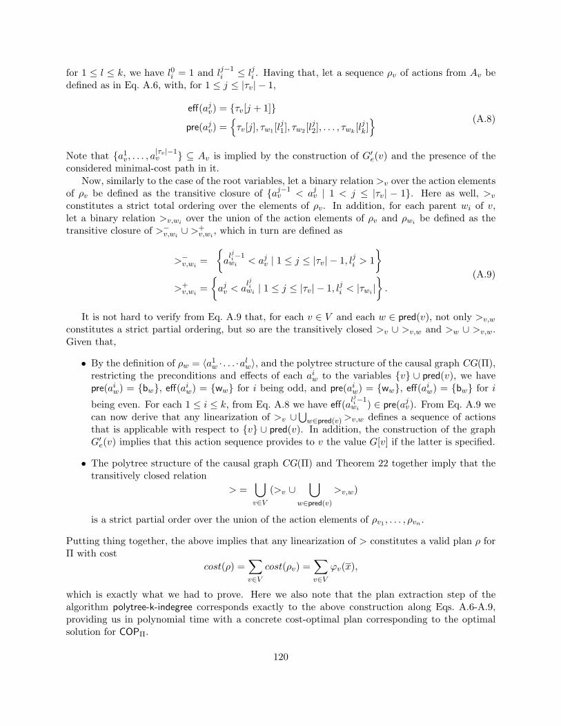
for 1 ≤ l ≤ k, we have l0i = 1 and lj−1i ≤ lji . Having that, let a sequence ρv of actions from Av be
defined as in Eq. A.6, with, for 1 ≤ j ≤ |τv| − 1,
eff(ajv) = {τv[j + 1]}pre(ajv) =
{τv[j], τw1 [lj1], τw2 [lj2], . . . , τwk [ljk]
} (A.8)
Note that {a1v, . . . , a
|τv |−1v } ⊆ Av is implied by the construction of G′e(v) and the presence of the
considered minimal-cost path in it.Now, similarly to the case of the root variables, let a binary relation >v over the action elements
of ρv be defined as the transitive closure of {aj−1v < ajv | 1 < j ≤ |τv| − 1}. Here as well, >v
constitutes a strict total ordering over the elements of ρv. In addition, for each parent wi of v,let a binary relation >v,wi over the union of the action elements of ρv and ρwi be defined as thetransitive closure of >−v,wi ∪ >+
v,wi , which in turn are defined as
>−v,wi ={alji−1wi < ajv | 1 ≤ j ≤ |τv| − 1, lji > 1
}>+v,wi =
{ajv < a
ljiwi | 1 ≤ j ≤ |τv| − 1, lji < |τwi |
}.
(A.9)
It is not hard to verify from Eq. A.9 that, for each v ∈ V and each w ∈ pred(v), not only >v,wconstitutes a strict partial ordering, but so are the transitively closed >v ∪ >v,w and >w ∪ >v,w.Given that,
• By the definition of ρw = 〈a1w · . . . ·alw〉, and the polytree structure of the causal graph CG(Π),
restricting the preconditions and effects of each aiw to the variables {v} ∪ pred(v), we havepre(aiw) = {bw}, eff(aiw) = {ww} for i being odd, and pre(aiw) = {ww}, eff(aiw) = {bw} for i
being even. For each 1 ≤ i ≤ k, from Eq. A.8 we have eff(alji−1wi ) ∈ pre(ajv). From Eq. A.9 we
can now derive that any linearization of >v ∪⋃w∈pred(v)>v,w defines a sequence of actions
that is applicable with respect to {v} ∪ pred(v). In addition, the construction of the graphG′e(v) implies that this action sequence provides to v the value G[v] if the latter is specified.
• The polytree structure of the causal graph CG(Π) and Theorem 22 together imply that thetransitively closed relation
> =⋃v∈V
(>v ∪⋃
w∈pred(v)
>v,w)
is a strict partial order over the union of the action elements of ρv1 , . . . , ρvn .
Putting thing together, the above implies that any linearization of > constitutes a valid plan ρ forΠ with cost
cost(ρ) =∑v∈V
cost(ρv) =∑v∈V
ϕv(x),
which is exactly what we had to prove. Here we also note that the plan extraction step of thealgorithm polytree-k-indegree corresponds exactly to the above construction along Eqs. A.6-A.9,providing us in polynomial time with a concrete cost-optimal plan corresponding to the optimalsolution for COPΠ.
120
(II) We now prove that if Π is solvable, then we must have α < ∞. Assume to the contrary thatthis is not the case. Let Π be a solvable planning task, and let ρ be an irreducible plan for Π.Given such ρ, let xρ = {τv1 , . . . , τvn} be an COP assignment with each |τvi | = |ρ↓vi | − 1. Notethat xρ is well-defined (that is, for 1 ≤ i ≤ n, we have τvi ∈ �∗[τ(vi)]) by the definition of τ(vi),Corollary 1, and ρ being irreducible. Let us now show that
∑ϕ∈F ϕ(xρ) ≤ cost(ρ), contradicting
our assumption that α =∞ due to α ≤∑ϕ∈F ϕ(xρ) and cost(ρ) <∞.
First, for each variable v with pred(v) = ∅, Eq. A.3 immediately implies ϕv(xρ) ≤ cost(ρ↓v).Next, for each non-root variable v ∈ V with pred(v) = {w1, . . . , wk}, consider the graph G′e(v)constructed with respect to τw1 , . . . , τwk . Let {a1, . . . , a|ρ↓v |} be the actions of ρ↓v numbered in theorder of their appearance along ρ↓v. Let {yw1(1), . . . , ywk(1)} denote the prevail condition of a1 witheach ywi(1) being time-stamped with its earliest appearance along τwi , that is, ywi(1) ∈ {b1
wi ,w1wi}.
Now, for 2 ≤ j ≤ |ρ↓v |, we set {yw1(j), . . . , ywk(j)} to the prevail condition of ai with each ywi(j)being time-stamped with the lowest possible time index along τwi satisfying “ywi(j − 1) does notcome after ywi(j) along τwi”. Given that
(i) ρ↓v is a complete order-preserving restriction of ρ to the v-changing actions Av,
(ii) the sequence of time-stamped prevail conditions {{yw1(j), . . . , ywk(j)}}|ρ↓v |j=1 is constructed asabove, and
(iii) |ρ↓v | = |τv| − 1 by the construction of xρ,
we have that G′e(v) contains a path
〈b1w1· · · b1
wk〉 → 〈yw1(1)· · · ywk(1)〉 → . . .→ 〈yw1(|ρ↓v |)· · ·ywk(|ρ↓v |)〉
and the cost of this path is cost(ρ↓v) <∞. However, from the constructive definition of ϕv in thealgorithm polytree-k-indegree, we have ϕv(xρ) being the cost of the minimal-cost path of |τv| − 1edges in G′e(v) originated in 〈b1
w1· · · b1
wk〉, and thus ϕv(xρ) ≤ cost(ρ↓v). The latter argument is
valid for all planning variables v ∈ V , and thus we have
∑ϕ∈F
ϕ(xρ) ≤∑v∈V
cost(ρ↓v) = cost(ρ),
which is what we had to prove.
121
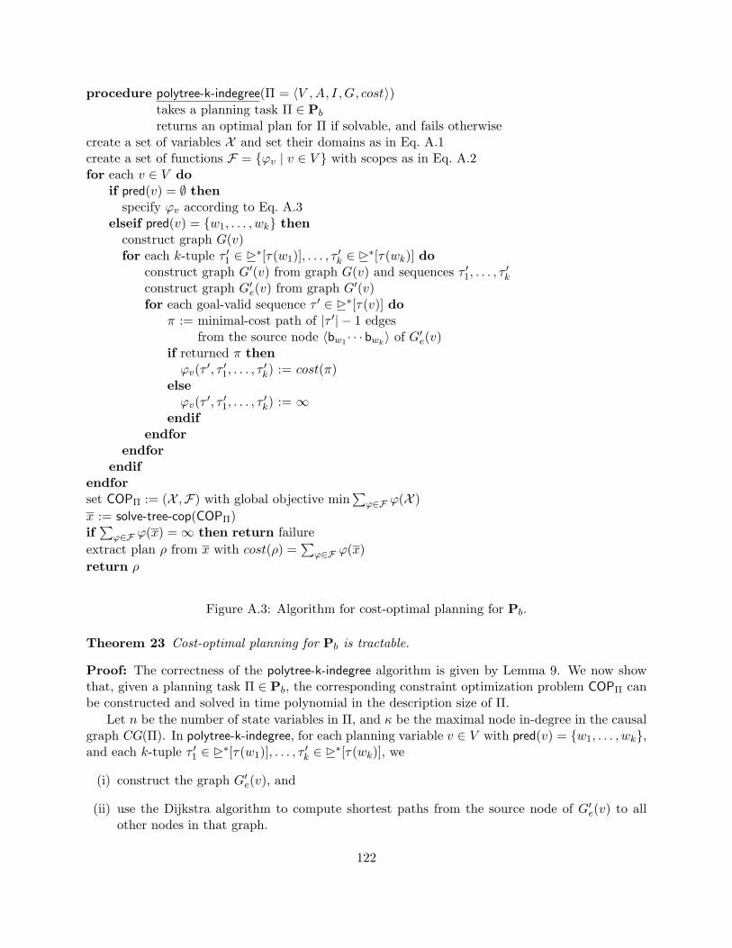
procedure polytree-k-indegree(Π = 〈V ,A, I ,G, cost〉)takes a planning task Π ∈ Pb
returns an optimal plan for Π if solvable, and fails otherwisecreate a set of variables X and set their domains as in Eq. A.1create a set of functions F = {ϕv | v ∈ V } with scopes as in Eq. A.2for each v ∈ V do
if pred(v) = ∅ thenspecify ϕv according to Eq. A.3
elseif pred(v) = {w1, . . . , wk} thenconstruct graph G(v)for each k-tuple τ ′1 ∈ �∗[τ(w1)], . . . , τ ′k ∈ �∗[τ(wk)] do
construct graph G′(v) from graph G(v) and sequences τ ′1, . . . , τ′k
construct graph G′e(v) from graph G′(v)for each goal-valid sequence τ ′ ∈ �∗[τ(v)] do
π := minimal-cost path of |τ ′| − 1 edgesfrom the source node 〈bw1 · · · bwk〉 of G′e(v)
if returned π thenϕv(τ ′, τ ′1, . . . , τ
′k) := cost(π)
elseϕv(τ ′, τ ′1, . . . , τ
′k) := ∞
endifendfor
endforendif
endforset COPΠ := (X ,F) with global objective min
∑ϕ∈F ϕ(X )
x := solve-tree-cop(COPΠ)if∑
ϕ∈F ϕ(x) =∞ then return failureextract plan ρ from x with cost(ρ) =
∑ϕ∈F ϕ(x)
return ρ
Figure A.3: Algorithm for cost-optimal planning for Pb.
Theorem 23 Cost-optimal planning for Pb is tractable.
Proof: The correctness of the polytree-k-indegree algorithm is given by Lemma 9. We now showthat, given a planning task Π ∈ Pb, the corresponding constraint optimization problem COPΠ canbe constructed and solved in time polynomial in the description size of Π.
Let n be the number of state variables in Π, and κ be the maximal node in-degree in the causalgraph CG(Π). In polytree-k-indegree, for each planning variable v ∈ V with pred(v) = {w1, . . . , wk},and each k-tuple τ ′1 ∈ �∗[τ(w1)], . . . , τ ′k ∈ �∗[τ(wk)], we
(i) construct the graph G′e(v), and
(ii) use the Dijkstra algorithm to compute shortest paths from the source node of G′e(v) to allother nodes in that graph.
122
For each wi, we have τ(wi) = n, and thus the number of k-tuples as above for each v ∈ V isO(nk). For each such k-tuple, the corresponding graph G′e(v) can be constructed in time linearin the number of its edges = O(n2k+2 · |Av|2) = O(n2k+2 · 22k+2) (Brafman & Domshlak, 2003).The time complexity of the Dijkstra algorithm on a digraph G = (N,E) is O(E log (N)), and onG′e(v) it gives us O
(n2k+2 · 22k+2 · log
(nk+1 · 2k+1
)). Putting things together, the complexity of
constructing COPΠ isO(n3κ+3 · 22κ+2 · log
(nκ+1 · 2κ+1
)). (A.10)
Applying a tree-decomposition of COPΠ along the scopes of its functional components we arriveinto an equivalent, tree-structured constraint optimization problem over n variables with domainsof size O(nκ+1). This COP is defined by the hard binary “compatibility” constraints betweenthe variables, and costs associated with the variables’ values. Such a tree-structured COP can besolved in time O(xy2) where x is the number of variables and y is an upper bound on the size ofa variable’s domain (Dechter, 2003). Therefore, solving our COPΠ can be done in time O(n2κ+3).As the expression in Eq. A.10 dominates both O(n2κ+3), and the time complexity of extracting aplan from the optimal solution to COPΠ (see the proof of (I) in Lemma 9), the overall complexityof the algorithm polytree-k-indegree is given by Eq. A.10. And since in Pb we have κ = O(1), weconclude that the complexity of polytree-k-indegree is polynomial in the description size of Π.
A.2 Cost-Optimal Planning for P(1) with Uniform-Cost Actions
In this section we provide a polynomial time algorithm for cost-optimal planning for P(1) prob-lems with uniform-cost actions. We begin with showing that such problems exhibit an interestingproperty, then we exploit this property for devising a planning-to-COP scheme for these problems,and then prove the correctness and complexity of the algorithm.
Here as well, we begin with providing some notation. Given a P(1) planning task Π =〈V ,A, I ,G, cost〉, for each v ∈ V , each w ∈ pred(v), and each α ∈ {bv,wv}, β ∈ {bw,ww}, byaα|β we denote the action a with eff(a)[v] = α and pre(a)[w] = β. Since Π is 1-dependent, theapplicability of aα|β is prevailed only by the value of w. It is important to keep in mind that aα|βis just a notation; the action aα|β may not belong to the action set A of Π.
A.2.1 Post-Unique Plans and P(1) Problems
We now proceed with introducing the notion of post-unique action sequences that plays a key rolein our planning-to-COP compilation here.
Definition 21 Let Π = 〈V ,A, I ,G, cost〉 be a ub planning task. An action sequence % ∈ A∗ iscalled post-unique if, for each pair of actions a, a′ ∈ %, we have eff(a) = eff(a′) only if a = a′.That is, all the changes of each variable to a certain value along % are performed by the same (typeof) action. The (possibly empty) set of all post-unique plans for Π is denoted by Pc(Π) (orsimply Pc, if the identity of Π is clear from the context).
The notion of post-unique action sequences is closely related to the notion of post-unique plan-ning problems (Backstrom & Klein, 1991; Backstrom & Nebel, 1995), but is considerably weakerthan the latter. While action sets of post-unique planning problems are not allowed to contain twoactions with the same effect, Definition 21 poses a similar restriction only on action sequences, and
123
not on the underlying planning problems. Still, the property of post-uniqueness for plans is strong.In general, solvable problems in ub may not exhibit post-unique plans at all. Turns out, however,that for the problems in P(1) this is very much not the case.
Theorem 24 For any solvable P(1) task Π = 〈V ,A, I ,G, cost〉, we have Pc(Π) 6= ∅. Moreover, ifthe actions A are uniform-cost, then Pc(Π) contains at least one cost-optimal plan.
Proof: As the correctness of the second claim immediately implies the correctness of the first one,here we focus on the proof the second claim. Given a P(1) planning task Π = 〈V ,A, I ,G, cost〉with uniform-cost actions, and plan ρ = 〈a1, . . . , am〉 for Π, we construct a sequence of actions ρ∗
• ρ∗ is a post-unique plan for Π,
• cost(ρ∗) = cost(ρ).
This construction is two-step. First, for each v ∈ V , we map the subsequence ρ↓v= 〈ai1 , . . . , aik〉into a post-unique sequence of actions ρ∗v = 〈a∗i1 , . . . , a∗ik〉. Note that the indexes i1, . . . , ik of theaction elements of each ρ↓v are the global indexes of these actions along ρ, and exactly the sameindexes are used for marking the elements of the constructed sequences ρ∗v. Having constructedthe sequences ρ∗v1
, . . . , ρ∗vn , we then merge them into a single actions sequence ρ∗, and show thatρ∗ is a valid plan for Π. The two properties of ρ∗ as required above will then hold immediatelybecause |ρ∗| = |ρ|, and post-uniqueness of ρ∗ is implied by the individual post-uniqueness of all itsper-variable components ρ∗v.
The mapping of subsequences ρ↓v of ρ to the desired sequences ρ∗v for all variables v is performedtop-down, consistently with a topological ordering of the causal graph CG(Π). This top-downprocessing allows us to assume that, when constructing ρ∗v, the subsequences ρ∗w for all w ∈ pred(v)are already constructed. Given that, while mapping each ρ↓v= 〈ai1 , . . . , aik〉 to the correspondingρ∗v, we distinguish between the following three cases.
(1) The subsequence ρ↓v is already post-unique.
In this case, we simply set ρ∗v to ρ↓v. In addition, we construct the following sets of orderingconstraints. First, we set a binary relation >v over the action elements of ρ∗v = 〈a∗i1 , . . . , a∗ik〉 to
>v= {a∗i < a∗j | a∗i , a∗j ∈ ρ∗v, i < j}. (A.11)
It is immediate from Eq. A.11 that >v is a strict total order over the elements of ρ∗v as >vsimply follows the action indexing inherited by ρ∗v from plan ρ via ρ↓v.Now, for each w ∈ pred(v), we set a binary relation >v,w over the elements of ρ∗v and ρ∗w to
>v,w=
(Sa∗i ∈ρ
∗v,a∗j∈ρ∗w{a∗i < a∗j | i < j} ∪ {a∗j < a∗i | j < i}, pre(a)[w] is specified for some a ∈ ρ∗v
∅, otherwise. (A.12)
For each w ∈ pred(v), the relation >v,w defined by Eq. A.12 is a strict total order over itsdomain because the ordering constraints between the elements of ρ∗v and ρ∗w are a subset ofthe constraints induced by the total-order plan ρ over the (corresponding) actions from ρ↓vand ρ↓w. For the same reason, from Eqs. A.11 and A.12, we have that, for each w ∈ pred(v),>v ∪ >v,w is a strict total order over the union of the elements of ρ∗v and ρ∗w.
From Eqs. A.11-A.12 we can now derive that any linearization of >v ∪⋃w∈pred(v)>v,w defines
a sequence of actions that is applicable with respect to {v} ∪ pred(v). In addition, |ρ∗v| = |ρ↓v |implies that this action sequence provides to v the value G[v] if the latter is specified.
124
(2) The subsequence ρ↓v is not post-unique, but the actions in ρ↓v are all prevailed by the value ofa single parent w ∈ pred(v).
Since ρ↓v is not post-unique, ρ↓v in this case has to contain instances of at least three actiontypes from {abv |bw , abv |ww , awv |bw , awv |ww}. Thus, in particular, it must be that
(a) |ρw↓|≥ 1, and
(b) for some β ∈ {bw,ww}, we have awv |β, abv |β ∈ ρ↓v.
Given that, we set ρ∗v = 〈a∗i1 , . . . , a∗ik〉 to
∀1 ≤ j ≤ k : a∗ij =
{awv |β, j is oddabv |β, j is even
.
Both post-uniqueness of such ρ∗v, as well as its applicability with respect to v are straightforward.The ordering constraints >v are then set according to Eq. A.11. Likewise, if ρ∗w = 〈aj1 , . . . , ajl〉,we set
>v,w=
⋃a∗i∈ρ∗v
{a∗i < aj1}, β = bw⋃a∗i∈ρ∗v
{a∗i > aj1}, β = ww, l = 1⋃a∗i∈ρ∗v
{a∗i > aj1} ∪ {a∗i < aj2}, β = ww, l > 1
(A.13)
Finally, the ordering constraints >v,w′ for the rest of the parents w′ ∈ pred(v) \ {w} are set toempty sets.
The relation >v here is identical to this in case (1), and thus it is a strict total order over theelements of ρ∗v. From Eq. A.13, it is easy to verify that >v,w is also a strict partial order overthe union of the elements of ρ∗v and ρ∗w. Finally, as all the elements of ρ∗v are all identicallyconstrained with respect to the elements of ρ∗w, we have >v ∪ >v,w forming a strict partialorder over the union of the elements of ρ∗v and ρ∗w. (For all other parents w′ ∈ pred(v), wesimply have >v ∪ >v,w = >v.)
From Eqs. A.11 and A.13 we can now derive that any linearization of >v ∪⋃w∈pred(v)>v,w
defines a sequence of actions that is applicable with respect to {v} ∪ pred(v). In addition,|ρ∗v| = |ρ↓v | implies that this action sequence provides to v the value G[v] if the latter isspecified.
(3) The subsequence ρ↓v is not post-unique, and the actions of ρ↓v are prevailed by more than oneparent of v.
The setting of this case in particular implies that there is a pair of v’s parents {u,w} ⊆ pred(v)such that awv |α, abv |β ∈ ρv for some α ∈ {bu,wu}, β ∈ {bw,ww}. Given that, we set ρ∗v to
∀1 ≤ j ≤ k : a∗ij =
{awv |α, j is oddabv |β, j is even
,
and, similarly to case (2), both post-uniqueness of ρ∗v, and its applicability with respect to vare straightforward.
125
Here as well, the ordering constraints >v are set according to Eq. A.11. Likewise, if ρ∗w =〈aj1 , . . . , ajl〉, and ρ∗u = 〈aj′1 , . . . , aj′l′ 〉, we set >v,w according to Eq. A.13 above, and >v,uaccording to Eq. A.14 below.
>v,u =
⋃a∗i∈ρ∗v
{a∗i < aj′1}, α = bu⋃a∗i∈ρ∗v
{a∗i > aj′1}, α = wu, l′ = 1⋃
a∗i∈ρ∗v{a∗i > aj′1} ∪ {a
∗i < aj′2}, α = wu, l
′ > 1
(A.14)
Finally, the ordering constraints >v,w′ for the rest of the parents w′ ∈ pred(v) \ {u,w} are setto empty sets.
The relation >v here is identical to this in cases (1-2), and relations >v,u and >v,w are effectivelyidentical to the relation >v,w in case (2). Thus, we have >v ∪ >v,u and >v ∪ >v,w formingstrict partial orders over the unions of the elements of ρ∗v and ρ∗u, and ρ∗v and ρ∗w, respectively.
From Eqs. A.11, A.13, and A.14 we can now derive that any linearization of>v ∪⋃w∈pred(v)>v,w
defines a sequence of actions that is applicable with respect to {v} ∪ pred(v). In addition,|ρ∗v| = |ρ↓v | implies that this action sequence provides to v the value G[v] if the latter isspecified.
As the last step, we now prove that, for each v ∈ V and each w ∈ pred(v), we have >w ∪ >v,wbeing a strict partial order over the union of the elements of ρ∗w and ρ∗v.
- If >v,w is constructed according to Eq. A.12, then >w ∪ >v,w is a subset of the constraintsinduced by plan ρ over the (corresponding to ρ∗v and ρ∗w) actions from ρv and ρw.
- Otherwise, if >v,w is constructed according to Eq. A.13 or (for us here identical) Eq. A.14,then >v,w (i) addresses at most two elements of ρw, (ii) orders these elements consistentlywith >w.
In both cases, the argued properties of >w ∪ >v,w implies that it forms a strict partial order overthe union of the elements of ρ∗v and ρ∗w.
Until now, we have specified the sequences ρ∗v, the orders >v induced by these sequences, theorders >v,w, and proved that all >v ∪ >v,w and >w ∪ >v,w form strict partial orders over theirdomains. This construction allows us to apply now Theorem 22 to the (considered as sets) sequencesρ∗v and orders >v and >v,w, proving that
>=⋃v∈V
(>v ∪⋃
w∈pred(v)
>v,w)
forms a strict partial order over the union of ρ∗v1, . . . , ρ∗vn . Putting thing together, the above
implies that any linearization ρ∗ of > is a plan for Π, and post-uniqueness of all its subsequencesρ∗v1
, . . . , ρ∗vn then implies ρ∗ ∈ Pc(Π). Moreover, if ρ is an optimal plan for Π, then |ρ∗| = |ρ| impliesthe optimality of ρ∗.
A.2.2 Construction
The main impact of Theorem 24 on our planning-to-COP scheme for uniform-cost P(1) is that wecan now restrict our attention to post-unique plans only. Given that, the constraint optimization
126
problem COPΠ = (X ,F) for a uniform-cost planning task Π = 〈V ,A, I ,G, cost〉 ∈ P(1) is specifiedas follows.
The variable set X contains a variable xv for each planning variable v ∈ V , and a variable xwvfor each edge (w, v) ∈ CG(Π). That is,
X = X V ∪ X E ,X V = {xv | v ∈ V }X E = {xwv | (w, v) ∈ CG(Π)}
(A.15)
For each variable xv ∈ X V , the domain D(xv) consists of all goal-valid prefixes of σ(v). Foreach variable xwv ∈ X E , the domain D(xwv ) consists of all triples of integers Jδw, δb, ηK satisfyingEq. A.16.
D(xv) = �∗[σ(v)]D(xwv ) = {Jδw, δb, ηK | δw, δb ∈ {0, 1}, 0 ≤ η ≤ n}
(A.16)
The semantics of Eq. A.16 is as follows. Let {w1, . . . , wk} be an arbitrary fixed ordering ofpred(v). If xv takes the value σv ∈ D(xv), then v is forced to provide σv sequence of values. Inturn, if xwiv takes the value Jδw, δb, ηK, then η corresponds to the number of value changes of v,δw = 1 (δb = 1) forces the subset of parents {w1, . . . , wi} ⊆ pred(v) to support (that is, prevail)all the changes of v to wv (respectively, to bv), and δw = 0 (δb = 0) relieves this subset of parents{w1, . . . , wi} from this responsibility.
For each variable x ∈ X , the set F contains a non-negative, real-valued function ϕx with thescope
Qx =
{xv}, x = xv, k = 0{xv, xwkv }, x = xv, k > 0{xw1
v , xw1}, x = xw1v , k > 0
{xwjv , xwj−1v , xwj}, x = x
wjv , 1 < j ≤ k
(A.17)
where pred(v) = {w1, . . . , wk} (and k = 0 means pred(v) = ∅). Proceeding now with specifying thesefunctional components F of COPΠ, first, for each xv with pred(v) = ∅, and for each σv ∈ �∗[σ(v)],we set ϕxv(σv) to
ϕxv (σv) =
0, |σv| = 1,1, (|σv| = 2) ∧ (awv ∈ Av),|σv| − 1, (|σv| > 2) ∧ (awv , abv ∈ Av),∞, otherwise
(A.18)
In turn, for each planning variable v ∈ V with pred(v) = {w1, . . . , wk}, k > 0, the function ϕxvis set to
ϕxv (σv, Jδw, δb, ηK) =
0, (|σv| = 1) ∧ (Jδw, δb, ηK = J0, 0, 0K),1, (|σv| = 2) ∧ (Jδw, δb, ηK = J1, 0, 1K),|σv| − 1, (|σv| > 2) ∧ (Jδw, δb, ηK = J1, 1, |σv| − 1K),∞, otherwise
(A.19)
127
The functions ϕxv capture the, marginal over the actions Av, cost of providing a sequence σvof value changes of v in Π, given that (in case of Eq. A.19) the parents of v are “ready to supportthese value changes”. In specifying the remaining functional components we use an “indicator”function ϕ specified in Eq. A.20.
ϕ (Jδw, δb, ηK, σw) =
8>>>>>>>>>>><>>>>>>>>>>>:
0, δw = 0, δb = 0,
0, δw = 1, δb = 0, (awv|bw ∈ Av) ∨ ((|σw| > 1) ∧ (awv|ww ∈ Av)),
0, δw = 0, δb = 1, (abv|bw ∈ Av) ∨ ((|σw| > 1) ∧ (abv|ww ∈ Av)),
0, δw = 1, δb = 1, (awv|bw , abv|bw ∈ Av) ∨ ((|σw| > 1) ∧ (awv|ww , abv|ww ∈ Av)),
0, δw = 1, δb = 1, |σw| ≥ η, awv|bw , abv|ww ∈ Av,0, δw = 1, δb = 1, |σw| > η, awv|ww , abv|bw ∈ Av,∞, otherwise
(A.20)
The semantics of ϕ is that, for each planning variable v ∈ V , each w ∈ pred(v), and each(Jδw, δb, ηK, σw) ∈ D(xwv )×D(xw), we have ϕ(Jδw, δb, ηK, σw) = 0 if the value sequence σw of w cansupport all the changes of v to wv (if δw = 1) and all the changes of v to bv (if δb = 1), out of ηvalue changes of v in Π. Given this indicator function ϕ, for each v ∈ V , the functional componentϕxw1
vis specified as
ϕxw1v
(Jδw, δb, ηK, σw1) = ϕ (Jδw, δb, ηK, σw1) , (A.21)
and the rest of the functions ϕxw2v, . . . , ϕxwkv are specified as follows. For each 2 ≤ i ≤ k, the
value of the function ϕxwjv
at the combination of Jδw, δb, ηK ∈ D(xwiv ), Jδ′w, δ′b, η′K ∈ D(xwi−1
v ), andσwi ∈ D(xwi) = �∗[σ(wi)] is specified as
ϕxwiv
`Jδw, δb, ηK, Jδ′w, δ
′b, η′K, σwj
´=
(ϕ`Jδw − δ′w, δb − δ′b, ηK, σwj
´, η = η′ ∧ δw ≥ δ′w ∧ δb ≥ δ′b
∞ otherwise(A.22)
This finalized the construction of COPΠ, and this construction constitutes the first three stepsof the algorithm polytree-1-dep-uniform in Figure A.4(a). The subsequent steps of this algorithmare conceptually similar to these of the polytree-k-indegree algorithm in Section A.1, with the majordifference being in the plan reconstruction routines. It is not hard to verify from Eqs. A.15-A.17,and the fact that the causal graph of Π ∈ P(1) forms a polytree that
(i) for each variable x ∈ X , |D(x)| = poly(n),
(ii) the tree-width of the cost network of F is ≤ 3, and
(iii) the optimal tree-decomposition of the COPΠ’s cost network is given by any topological orderingof the causal graph that is consistent with the (arbitrary yet fixed at the time of the COPΠ’sconstruction) orderings of each planning variable’s parents in the causal graph.
For an illustration, we refer the reader to Figure 3.3 (pp. 23) where Figure 3.3(a) depicts the causalgraph of a planning task Π ∈ P(1), and Figure 3.3(c) depicts the cost network of the correspondingCOPΠ. The top-most variables and the cliques in the cost network correspond to the functionalcomponents of COPΠ.
128
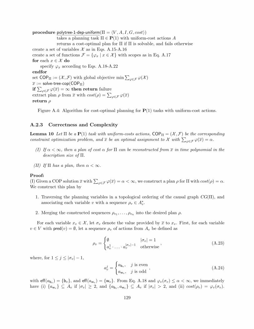
procedure polytree-1-dep-uniform(Π = 〈V ,A, I ,G, cost〉)takes a planning task Π ∈ P(1) with uniform-cost actions Areturns a cost-optimal plan for Π if Π is solvable, and fails otherwise
create a set of variables X as in Eqs. A.15-A.16create a set of functions F = {ϕx | x ∈ X} with scopes as in Eq. A.17for each x ∈ X do
specify ϕx according to Eqs. A.18-A.22endforset COPΠ := (X ,F) with global objective min
∑ϕ∈F ϕ(X )
x := solve-tree-cop(COPΠ)if∑
ϕ∈F ϕ(x) =∞ then return failureextract plan ρ from x with cost(ρ) =
∑ϕ∈F ϕ(x)
return ρ
Figure A.4: Algorithm for cost-optimal planning for P(1) tasks with uniform-cost actions.
A.2.3 Correctness and Complexity
Lemma 10 Let Π be a P(1) task with uniform-costs actions, COPΠ = (X ,F) be the correspondingconstraint optimization problem, and x be an optimal assignment to X with
∑ϕ∈F ϕ(x) = α.
(I) If α <∞, then a plan of cost α for Π can be reconstructed from x in time polynomial in thedescription size of Π.
(II) If Π has a plan, then α <∞.
Proof:(I) Given a COP solution x with
∑ϕ∈F ϕ(x) = α <∞, we construct a plan ρ for Π with cost(ρ) = α.
We construct this plan by
1. Traversing the planning variables in a topological ordering of the causal graph CG(Π), andassociating each variable v with a sequence ρv ∈ A∗v.
2. Merging the constructed sequences ρv1 , . . . , ρvn into the desired plan ρ.
For each variable xv ∈ X , let σv denote the value provided by x to xv. First, for each variablev ∈ V with pred(v) = ∅, let a sequence ρv of actions from Av be defined as
ρv =
{∅ |σv| = 1a1v · . . . · a|σv |−1
v otherwise, (A.23)
where, for 1 ≤ j ≤ |σv| − 1,
ajv =
{abv , j is evenawv , j is odd
, (A.24)
with eff(abv) = {bv}, and eff(awv) = {wv}. From Eq. A.18 and ϕv(σv) ≤ α < ∞, we immediatelyhave (i) {awv} ⊆ Av if |σv| ≥ 2, and {abv , awv} ⊆ Av if |σv| > 2, and (ii) cost(ρv) = ϕv(σv).
129
Let a binary relation >v over the action elements of ρv be defined as the transitive closure of{aj−1
v < ajv | 1 < j ≤ |σv| − 1}, that is
>v= {aj′v < ajv | 1 ≤ j′ < j ≤ |σv| − 1} (A.25)
Clearly, >v constitutes a strict total ordering over the elements of ρv, making ρv an applicablesequence of actions that provides to v the value G[v] if the latter is specified.
Next, for each variable v ∈ V with pred(v) 6= ∅, let pred(v) = {w1, . . . , wk} be numberedaccording to their ordering used for constructing COPΠ. Likewise, for each wi ∈ pred(v), letJδw(i), δb(i), η(i)K be the value provided by x to xwiv . Given that, let a pair of indexes 0 ≤ 〈w〉, 〈b〉 ≤k be defined as
〈w〉 =
0, δw(k) = 0,1, δw(1) = 1,j, δw(j − 1) < δw(j), 2 ≤ j ≤ k
(A.26)
〈b〉 =
0, δb(k) = 0,1, δb(1) = 1,j, δb(j − 1) < δb(j), 2 ≤ j ≤ k
(A.27)
Informally, in our next-coming construction of the action sequence ρv for the state variable v, 〈w〉and 〈b〉 will indicate the parents prevailing the value changes of v to wv and to bv, respectively,along ρv. Note that Eqs. A.26-A.27 are well-defined because, for 2 ≤ j ≤ k, Eq. A.22 implies
δw(j − 1) ≤ δw(j) ∧ δb(j − 1) ≤ δb(j) ∧ η(j − 1) = η(j).
Given this notation, the action sequence ρv and the partial orders >v,w1 , . . . , >v,wk are con-structed as follows.
[ 〈w〉 = 0, 〈b〉 = 0 ] In this case, the constructed plan ρ should perform no value changes of v, andthus ρv is set to an empty action sequence, and, consequently, both >v and all >v,w are setto empty sets.
[ 〈w〉 > 0, 〈b〉 = 0 ] In this case, the constructed plan ρ should perform exactly one value change ofv (from bv to wv), and thus ρv is set to contain exactly one action a1
v with eff(a) = {wv}, and
pre(a1v) =
{{bv, bw〈w〉}, awv |bw〈w〉
∈ Av{bv,ww〈w〉}, otherwise
(A.28)
Note that a1v is well-defined, as α <∞ and Eq. A.20 together imply that {awv |bw〈w〉
, awv |bw〈w〉}∩
Av 6= ∅ (see case (2) in Eq. A.20). In both outcomes of Eq. A.28, we set >v= ∅. If a1v =
awv |bw〈w〉, we set
>v,w〈w〉= {a1v < a1
w〈w〉| a1
w〈w〉∈ ρw〈w〉} (A.29)
Otherwise, if a1v = awv |ww〈w〉
, then from case (2) in Eq. A.20, awv |bw〈w〉6∈ Av, and α < ∞, we
have |σw〈w〉 | > 1, and thus |ρw〈w〉 | ≥ 1. Given that, we set
>v,w〈w〉= {a1w〈w〉
< a1v} ∪ {a1
v < a2w〈w〉| a2
w〈w〉∈ ρw〈w〉} (A.30)
130
In both cases, it is easy to verify that >v ∪ >v,w〈w〉 ∪ >w〈w〉 constitutes a strict total orderover the action elements of ρv and ρw〈w〉 . (In particular, this trivially implies that >v ∪ >v,wand >v,w ∪ >w are strict partial orderings over their domains.)
From Eqs. A.25, A.29, and A.30 we can now derive that any linearization of>v ∪⋃w∈pred(v)>v,w
defines a sequence of actions that is applicable with respect to {v} ∪ pred(v). In addition,Eq. A.16 implies that this action sequence provides to v the value G[v] if the latter is specified.
[ 〈w〉 > 0, 〈b〉 > 0, 〈w〉 = 〈b〉 ] In this case, the constructed plan ρ should perform more than onevalue change of v, and all these value changes should be performed by (a pair of types of)actions prevailed by the value of w〈w〉. From α <∞, we have ϕ(Jδw(〈w〉), δb(〈w〉), ηK, σw〈w〉) =0. The specification of the case in question (that is, 〈w〉 = 〈b〉 > 0) thus implies that one ofthe conditions of the cases (4-6) of Eq. A.20 should hold. Given that, we distinguish betweenthe following four settings.
(1) If {awv |bw〈w〉, abv |bw〈w〉
} ⊆ Av, then ρv is specified according to Eq. A.23, and its actionelements are specified as
aiv =
awv |bw〈w〉, i is odd
abv |bw〈w〉, i is even
. (A.31)
The relation >v is set according to Eq. A.25, and >v,w〈w〉 is set to
>v,w〈w〉= {aiv < a1w〈w〉| aiv ∈ ρv, a1
w〈w〉∈ ρw〈w〉} (A.32)
Finally, for all w ∈ pred(v) \ {w〈w〉}, we set >v,w= ∅.(2) Otherwise, if {awv |ww〈w〉
, abv |ww〈w〉} ⊆ Av and |σw〈w〉 | > 1, then we have |ρw〈w〉 | ≥ 1. Given
that, we again set ρv according to Eq. A.23, but now with its action elements being setas
aiv =
awv |ww〈w〉, i is odd
abv |ww〈w〉, i is even
. (A.33)
The relation >v is set according to Eq. A.25, and >v,w〈w〉 is set to
>v,w〈w〉= {a1w〈w〉
< aiv | aiv ∈ ρv} ∪ {aiv < a2w〈w〉| aiv ∈ ρv, a2
w〈w〉∈ ρw〈w〉} (A.34)
Finally, here as well, for all w ∈ pred(v) \ {w〈w〉}, we set >v,w= ∅.(3) Otherwise, if {awv |bw〈w〉
, abv |ww〈w〉} ⊆ Av, and |σw〈w〉 | ≥ |σv| − 1, then ρv is specified
according to Eq. A.23, and its action elements are specified as
aiv =
awv |bw〈w〉, i is odd
abv |ww〈w〉, i is even
. (A.35)
The relation >v is set according to Eq. A.25, and >v,w〈w〉 is set to
>v,w〈w〉=⋃
aiv∈ρv ,ajw〈w〉∈ρw〈w〉
{aiv < ajw〈w〉 | i ≤ j} ∪ {ajw〈w〉
< aiv | i > j} (A.36)
For all w ∈ pred(v) \ {w〈w〉}, we set >v,w= ∅.
131
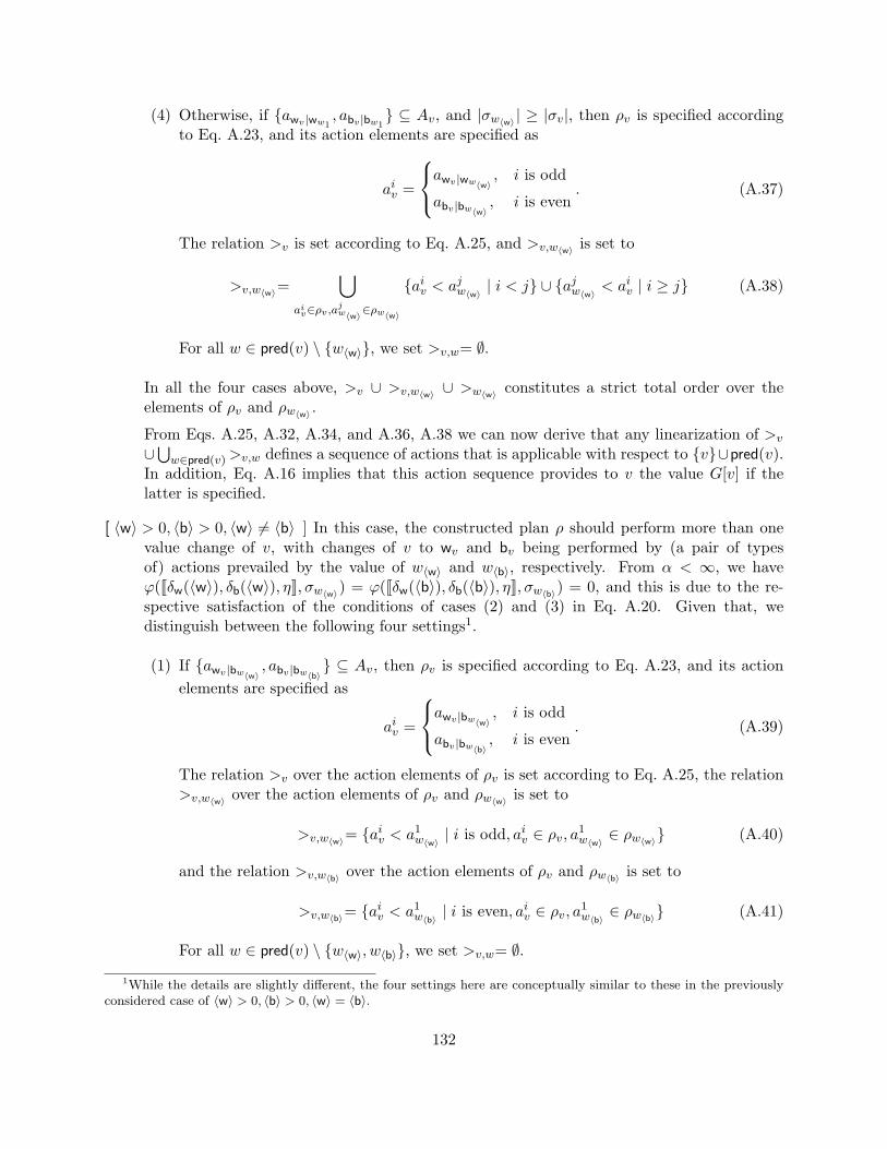
(4) Otherwise, if {awv |ww1, abv |bw1
} ⊆ Av, and |σw〈w〉 | ≥ |σv|, then ρv is specified accordingto Eq. A.23, and its action elements are specified as
aiv =
awv |ww〈w〉, i is odd
abv |bw〈w〉, i is even
. (A.37)
The relation >v is set according to Eq. A.25, and >v,w〈w〉 is set to
>v,w〈w〉=⋃
aiv∈ρv ,ajw〈w〉∈ρw〈w〉
{aiv < ajw〈w〉 | i < j} ∪ {ajw〈w〉 < aiv | i ≥ j} (A.38)
For all w ∈ pred(v) \ {w〈w〉}, we set >v,w= ∅.
In all the four cases above, >v ∪ >v,w〈w〉 ∪ >w〈w〉 constitutes a strict total order over theelements of ρv and ρw〈w〉 .
From Eqs. A.25, A.32, A.34, and A.36, A.38 we can now derive that any linearization of >v∪⋃w∈pred(v)>v,w defines a sequence of actions that is applicable with respect to {v}∪pred(v).In addition, Eq. A.16 implies that this action sequence provides to v the value G[v] if thelatter is specified.
[ 〈w〉 > 0, 〈b〉 > 0, 〈w〉 6= 〈b〉 ] In this case, the constructed plan ρ should perform more than onevalue change of v, with changes of v to wv and bv being performed by (a pair of typesof) actions prevailed by the value of w〈w〉 and w〈b〉, respectively. From α < ∞, we haveϕ(Jδw(〈w〉), δb(〈w〉), ηK, σw〈w〉) = ϕ(Jδw(〈b〉), δb(〈b〉), ηK, σw〈b〉) = 0, and this is due to the re-spective satisfaction of the conditions of cases (2) and (3) in Eq. A.20. Given that, wedistinguish between the following four settings1.
(1) If {awv |bw〈w〉, abv |bw〈b〉
} ⊆ Av, then ρv is specified according to Eq. A.23, and its actionelements are specified as
aiv =
awv |bw〈w〉, i is odd
abv |bw〈b〉, i is even
. (A.39)
The relation >v over the action elements of ρv is set according to Eq. A.25, the relation>v,w〈w〉 over the action elements of ρv and ρw〈w〉 is set to
>v,w〈w〉= {aiv < a1w〈w〉| i is odd, aiv ∈ ρv, a1
w〈w〉∈ ρw〈w〉} (A.40)
and the relation >v,w〈b〉 over the action elements of ρv and ρw〈b〉 is set to
>v,w〈b〉= {aiv < a1w〈b〉| i is even, aiv ∈ ρv, a1
w〈b〉∈ ρw〈b〉} (A.41)
For all w ∈ pred(v) \ {w〈w〉, w〈b〉}, we set >v,w= ∅.1While the details are slightly different, the four settings here are conceptually similar to these in the previously
considered case of 〈w〉 > 0, 〈b〉 > 0, 〈w〉 = 〈b〉.
132
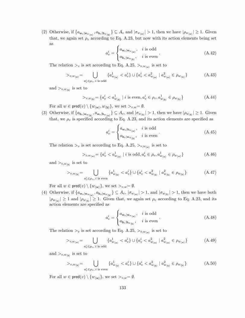
(2) Otherwise, if {awv |ww〈w〉, abv |bw〈b〉
} ⊆ Av and |σw〈w〉 | > 1, then we have |ρw〈w〉 | ≥ 1. Giventhat, we again set ρv according to Eq. A.23, but now with its action elements being setas
aiv =
awv |ww〈w〉, i is odd
abv |ww〈b〉, i is even
. (A.42)
The relation >v is set according to Eq. A.25, >v,w〈w〉 is set to
>v,w〈w〉=⋃
aiv∈ρv , i is odd
{a1w〈w〉
< aiv} ∪ {aiv < a2w〈w〉| a2
w〈w〉∈ ρw〈w〉} (A.43)
and >v,w〈b〉 is set to
>v,w〈b〉= {aiv < a1w〈b〉| i is even, aiv ∈ ρv, a1
w〈b〉∈ ρw〈b〉} (A.44)
For all w ∈ pred(v) \ {w〈w〉, w〈b〉}, we set >v,w= ∅.(3) Otherwise, if {abv |ww〈b〉
, awv |bw〈w〉} ⊆ Av, and |σw〈b〉 | > 1, then we have |ρw〈b〉 | ≥ 1. Given
that, we ρv is specified according to Eq. A.23, and its action elements are specified as
aiv =
awv |bw〈w〉, i is odd
abv |ww〈b〉, i is even
. (A.45)
The relation >v is set according to Eq. A.25, >v,w〈w〉 is set to
>v,w〈w〉= {aiv < a1w〈w〉| i is odd, aiv ∈ ρv, a1
w〈w〉∈ ρw〈w〉} (A.46)
and >v,w〈b〉 is set to
>v,w〈b〉=⋃
aiv∈ρv , i is even
{a1w〈b〉
< aiv} ∪ {aiv < a2w〈b〉| a2
w〈b〉∈ ρw〈b〉} (A.47)
For all w ∈ pred(v) \ {w〈w〉}, we set >v,w= ∅.(4) Otherwise, if {awv |ww〈w〉
, abv |ww〈b〉} ⊆ Av, |σw〈w〉 | > 1, and |σw〈b〉 | > 1, then we have both
|ρw〈w〉 | ≥ 1 and |ρw〈b〉 | ≥ 1. Given that, we again set ρv according to Eq. A.23, and itsaction elements are specified as
aiv =
awv |ww〈w〉, i is odd
abv |bw〈b〉, i is even
. (A.48)
The relation >v is set according to Eq. A.25, >v,w〈w〉 is set to
>v,w〈w〉=⋃
aiv∈ρv , i is odd
{a1w〈w〉
< aiv} ∪ {aiv < a2w〈w〉| a2
w〈w〉∈ ρw〈w〉} (A.49)
and >v,w〈b〉 is set to
>v,w〈b〉=⋃
aiv∈ρv , i is even
{a1w〈b〉
< aiv} ∪ {aiv < a2w〈b〉| a2
w〈b〉∈ ρw〈b〉} (A.50)
For all w ∈ pred(v) \ {w〈w〉}, we set >v,w= ∅.
133
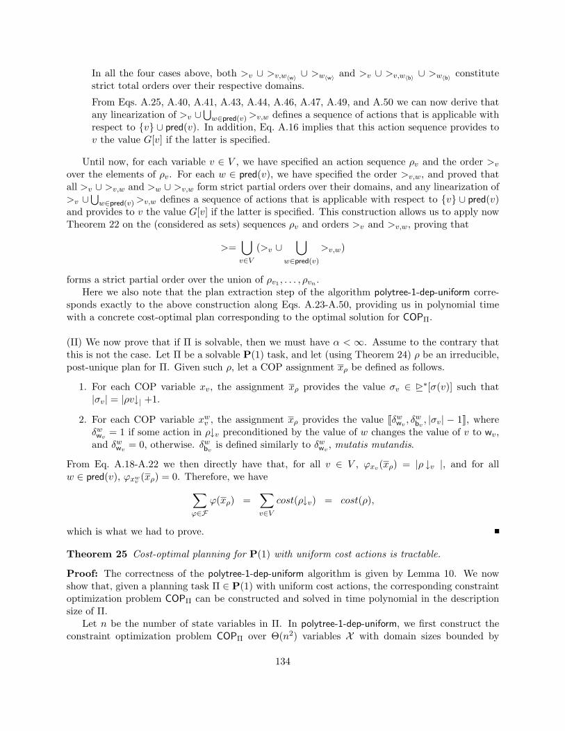
In all the four cases above, both >v ∪ >v,w〈w〉 ∪ >w〈w〉 and >v ∪ >v,w〈b〉 ∪ >w〈b〉 constitutestrict total orders over their respective domains.
From Eqs. A.25, A.40, A.41, A.43, A.44, A.46, A.47, A.49, and A.50 we can now derive thatany linearization of >v ∪
⋃w∈pred(v)>v,w defines a sequence of actions that is applicable with
respect to {v} ∪ pred(v). In addition, Eq. A.16 implies that this action sequence provides tov the value G[v] if the latter is specified.
Until now, for each variable v ∈ V , we have specified an action sequence ρv and the order >vover the elements of ρv. For each w ∈ pred(v), we have specified the order >v,w, and proved thatall >v ∪ >v,w and >w ∪ >v,w form strict partial orders over their domains, and any linearization of>v ∪
⋃w∈pred(v)>v,w defines a sequence of actions that is applicable with respect to {v} ∪ pred(v)
and provides to v the value G[v] if the latter is specified. This construction allows us to apply nowTheorem 22 on the (considered as sets) sequences ρv and orders >v and >v,w, proving that
>=⋃v∈V
(>v ∪⋃
w∈pred(v)
>v,w)
forms a strict partial order over the union of ρv1 , . . . , ρvn .Here we also note that the plan extraction step of the algorithm polytree-1-dep-uniform corre-
sponds exactly to the above construction along Eqs. A.23-A.50, providing us in polynomial timewith a concrete cost-optimal plan corresponding to the optimal solution for COPΠ.
(II) We now prove that if Π is solvable, then we must have α < ∞. Assume to the contrary thatthis is not the case. Let Π be a solvable P(1) task, and let (using Theorem 24) ρ be an irreducible,post-unique plan for Π. Given such ρ, let a COP assignment xρ be defined as follows.
1. For each COP variable xv, the assignment xρ provides the value σv ∈ �∗[σ(v)] such that|σv| = |ρv↓| +1.
2. For each COP variable xwv , the assignment xρ provides the value Jδwwv , δwbv, |σv| − 1K, where
δwwv = 1 if some action in ρ↓v preconditioned by the value of w changes the value of v to wv,and δwwv = 0, otherwise. δwbv is defined similarly to δwwv , mutatis mutandis.
From Eq. A.18-A.22 we then directly have that, for all v ∈ V , ϕxv(xρ) = |ρ ↓v |, and for allw ∈ pred(v), ϕxwv (xρ) = 0. Therefore, we have∑
ϕ∈Fϕ(xρ) =
∑v∈V
cost(ρ↓v) = cost(ρ),
which is what we had to prove.
Theorem 25 Cost-optimal planning for P(1) with uniform cost actions is tractable.
Proof: The correctness of the polytree-1-dep-uniform algorithm is given by Lemma 10. We nowshow that, given a planning task Π ∈ P(1) with uniform cost actions, the corresponding constraintoptimization problem COPΠ can be constructed and solved in time polynomial in the descriptionsize of Π.
Let n be the number of state variables in Π. In polytree-1-dep-uniform, we first construct theconstraint optimization problem COPΠ over Θ(n2) variables X with domain sizes bounded by
134
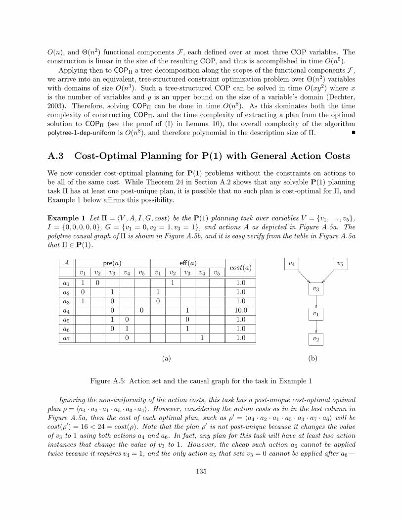
O(n), and Θ(n2) functional components F , each defined over at most three COP variables. Theconstruction is linear in the size of the resulting COP, and thus is accomplished in time O(n5).
Applying then to COPΠ a tree-decomposition along the scopes of the functional components F ,we arrive into an equivalent, tree-structured constraint optimization problem over Θ(n2) variableswith domains of size O(n3). Such a tree-structured COP can be solved in time O(xy2) where xis the number of variables and y is an upper bound on the size of a variable’s domain (Dechter,2003). Therefore, solving COPΠ can be done in time O(n8). As this dominates both the timecomplexity of constructing COPΠ, and the time complexity of extracting a plan from the optimalsolution to COPΠ (see the proof of (I) in Lemma 10), the overall complexity of the algorithmpolytree-1-dep-uniform is O(n8), and therefore polynomial in the description size of Π.
A.3 Cost-Optimal Planning for P(1) with General Action Costs
We now consider cost-optimal planning for P(1) problems without the constraints on actions tobe all of the same cost. While Theorem 24 in Section A.2 shows that any solvable P(1) planningtask Π has at least one post-unique plan, it is possible that no such plan is cost-optimal for Π, andExample 1 below affirms this possibility.
Example 1 Let Π = 〈V ,A, I ,G, cost〉 be the P(1) planning task over variables V = {v1, . . . , v5},I = {0, 0, 0, 0, 0}, G = {v1 = 0, v2 = 1, v3 = 1}, and actions A as depicted in Figure A.5a. Thepolytree causal graph of Π is shown in Figure A.5b, and it is easy verify from the table in Figure A.5athat Π ∈ P(1).
A pre(a) eff(a)cost(a)
v1 v2 v3 v4 v5 v1 v2 v3 v4 v5
a1 1 0 1 1.0a2 0 1 1 1.0a3 1 0 0 1.0a4 0 0 1 10.0a5 1 0 0 1.0a6 0 1 1 1.0a7 0 1 1.0
v4
��>>>>>>v5
��������
v3
��v1
��v2
(a) (b)
Figure A.5: Action set and the causal graph for the task in Example 1
Ignoring the non-uniformity of the action costs, this task has a post-unique cost-optimal optimalplan ρ = 〈a4 · a2 · a1 · a5 · a3 · a4〉. However, considering the action costs as in in the last column inFigure A.5a, then the cost of each optimal plan, such as ρ′ = 〈a4 · a2 · a1 · a5 · a3 · a7 · a6〉 will becost(ρ′) = 16 < 24 = cost(ρ). Note that the plan ρ′ is not post-unique because it changes the valueof v3 to 1 using both actions a4 and a6. In fact, any plan for this task will have at least two actioninstances that change the value of v3 to 1. However, the cheap such action a6 cannot be appliedtwice because it requires v4 = 1, and the only action a5 that sets v3 = 0 cannot be applied after a6—
135
a5 requires v4 = 0, and there is no action that have this effect. Therefore, any post-unique plan forthis task will have to invoke twice the action a4, and thus will have cost of at least 2 · cost(a4) = 20.
Fortunately, here we show that any solvable P(1) task is guaranteed to have a cost-optimal plansatisfying a certain “relaxation” of action sequence post-uniqueness that still allows us to devise a(more costly than polytree-1-dep-uniform) planning-to-COP scheme for general P(1) problems.
A.3.1 Post-3/2 Plans and P(1) Problems
We now proceed with introducing the notion of post-3/2 property for action sequences that relaxesthe post-uniqueness property exploited in the previous section.
Definition 22 Let Π = 〈V ,A, I ,G, cost〉 be a ub planning task. An action sequence % ∈ A∗ iscalled post-3/2 if, for each v ∈ V , a ∈ %v, there exist α 6= β ∈ {bv,wv}, a parent w ∈ pred(v),γ, δ ∈ {bw,ww}, and ξ ∈ {bu,wu | u ∈ pred(v)}, such that a ∈ {aα|γ , aβ|δ, aα|ξ}. That is, all thechanges of each variable are done using at most three types of actions which are prevailed by at mosttwo parents, and if u is different from w, then different actions prevailed by w perform differentvalue changes of v.
The (possibly empty) set of all post-3/2 plans for Π is denoted by P3/2(Π) (or simply P3/2,if the identity of Π is clear from the context).
To illustrate the rather involved definition of post-3/2 plans, consider the following four actionsequences of four actions each. The only value changes made by these sequences are changes ofvariable v with pred(v) = {x, y, z}.
• 〈awv |bx ·abv |wx ·awv |bx ·abv |by〉 is post-3/2 because it uses three types of actions, each prevailedby one of the two parents x, y.
• 〈awv |bx · abv |by · awv |bx · abv |by〉 is post-3/2 because it uses two types of actions, each prevailedby one of the two parents x, y.
• 〈awv |bx · abv |by · awv |bx · abv |bz〉 is not post-3/2 because it uses three types of actions, eachprevailed by one of the three parents x, y, z.
• 〈awv |bx · abv |wx · awv |by · abv |by〉 is not post-3/2 because it uses four types of actions, eachprevailed by one of the two parents x, y.
It is not hard to verify that post-3/2 is a relaxation of post-uniqueness—if a plan is post-unique,then it is post-3/2, but not necessarily the other way around. Turns out that, for any P(1) task Π,this relaxed property is guaranteed to be satisfied by at least one cost-optimal plan for Π.
Theorem 26 For every solvable P(1) planning task Π = 〈V ,A, I ,G, cost〉, the plan set P3/2(Π)contains at least one cost-optimal plan.
Proof: Given a P(1) task Π = 〈V ,A, I ,G, cost〉, and cost-optimal plan ρa1, . . . , am〉 for Π, weconstruct a sequence of actions ρ∗ such that:
• ρ∗ is a post-3/2 plan for Π,
• cost(ρ∗) = cost(ρ).
136
In nutshell, first, for each v ∈ V , we map the subsequence ρ[v] = 〈a1, . . . , ak〉 of ρ into a sequenceof actions ρ∗v = 〈a∗1, . . . , a∗k〉 that (i) satisfy the post-3/2 property, and (ii) cost(ρ∗v) ≤ cost(ρ[v]).Then, we merge the constructed sequences {ρ∗v}v∈V into ρ∗, and show that ρ∗ is a valid plan for Π.The two properties of ρ∗ as required above will then hold immediately because cost(ρ∗) = cost(ρ),and ρ∗ being post-3/2 is implied by all its per-variable components ρ∗v being post-3/2.
For each variable v ∈ V , with pred(v) = ∅, we set ρ∗v = ρ[v] and
>v= {ai < aj | ai, aj ∈ ρ[v], i < j}. (A.51)
It is immediate from Eq. A.51 that >v is a strict total order over the elements of ρ∗v.In turn, for each variable v ∈ V with pred(v) 6= ∅, given {σw}w∈pred(v), such that |σw| = |ρ[w]|+1,
let aαi be the i’th cheapest action that changes variable v to α ∈ {bv,wv} and prevailed by somevalue from {σw}w∈pred(v). Let us now focus on aw
1 = awv |γ , aw2 = awv |µ, ab
1 = abv |δ, ab2 = abv |ν .2
(I) If γ = δ ∈ {bw,ww}, we set
a∗i =
{awv |γ i = 2j − 1, j ∈ Nabv |γ otherwise
(A.52)
In addition, we construct the following sets of ordering constraints. First, we set a binaryrelation >v over the action elements of ρ∗v = 〈a∗1, . . . , a∗k〉 to
>v= {a∗i < a∗j | a∗i , a∗j ∈ ρ∗v, i < j}. (A.53)
It is immediate from Eq. A.53 that >v is a strict total order over the elements of ρ∗v. Likewise,if ρ∗w = 〈aj1 , . . . , ajl〉, we set
>v,w=
⋃a∗i∈ρ∗v
{a∗i < aj1}, γ = bw⋃a∗i∈ρ∗v
{a∗i > aj1}, γ = ww, l = 1⋃a∗i∈ρ∗v
{a∗i > aj1} ∪ {a∗i < aj2}, γ = ww, l > 1
(A.54)
Finally, the ordering constraints >v,w′ for the rest of the parents w′ ∈ pred(v) \ {w} are setto empty sets.
For each w ∈ pred(v), it is easy to verify that the relation >v,w defined by Eq. A.54 is astrict total order over its domain. Also, from Eqs. A.53 and A.54, we have that, for eachw ∈ pred(v), >v ∪ >v,w is a strict total order over the union of the elements of ρ∗v and ρ∗w.
From Eqs. A.53-A.54 we can now derive that any linearization of >v ∪⋃w∈pred(v)>v,w defines
a sequence of actions that is applicable with respect to {v}∪pred(v). In addition, |ρ∗v| = |ρ[v]|together with Eq. A.52 implies that this action sequence provides to v the value G[v] if thelatter is specified.
2It is possible that some of these actions do not exist, and our case by case analysis in the proof transparently takesthis possibility into account. Specifically, if aw
1 does not exist, then variable v simply unchangeable, meaning ρ[v] = ∅.Next, if ab
1 does not exist, then v can be changed at most once (from b to w), and this is covered by a subcase of(I). If aw
2 does not exist, and ab2 does exist, then only sub-cases (a) of the cases {(III), (IV )}.{1, 3, 5, 7} are possible.
Similarly, if ab2 does not exist, and aw
2 does exist, then only sub-cases (b) of the cases {(III), (IV )}.{1, 3, 5, 7} arepossible. Finally, if both aw
2 and ab2 do not exist, then cases {(III), (IV )}.{1, 3, 5, 7} are not possible at all.
137
(II) If γ ∈ {bw,ww} and δ ∈ {bu,wu}, such that w 6= u, we set
a∗i =
{awv |γ i = 2j − 1, j ∈ Nabv |δ otherwise
(A.55)
Here as well, the ordering constraints >v are set according to Eq. A.53. Likewise, if ρ∗w =〈a1, . . . , al〉, and ρ∗u = 〈a′1, . . . , a′l′〉, we set >v,w according to Eq. A.54 above, and >v,uaccording to Eq. A.56 below.
>v,u =
⋃a∗i∈ρ∗v
{a∗i < a′1}, ν = bu⋃a∗i∈ρ∗v
{a∗i > a′1}, ν = wu, l′ = 1⋃
a∗i∈ρ∗v{a∗i > a′1} ∪ {a∗i < a′2}, δ = wu, l
′ > 1
(A.56)
Finally, here as well, the ordering constraints >v,w′ for the rest of the parents w′ ∈ pred(v) \{u,w} are set to empty sets.
The relations >v here is identical to these in previous case, and relations >v,u and >v,ware effectively identical to the relation >v,w in previous case. Thus, here as well, we have>v ∪ >v,u and >v ∪ >v,w forming strict partial orders over the unions of the elements of ρ∗vand ρ∗u, and ρ∗v and ρ∗w, respectively.
From Eqs. A.53, A.54, A.56 we can now derive that any linearization of >v ∪⋃w∈pred(v)>v,w
defines a sequence of actions that is applicable with respect to {v} ∪ pred(v). In addition,|ρ∗v| = |ρ[v]| together with Eq. A.55 implies that this action sequence provides to v the valueG[v] if the latter is specified.
(III) If γ = bw, δ = ww, we distinguish between a few cases based on σw and σv.
(1) If |ρ[v]| = 2y+ 1, |σw| = 2x, |σw| ≤ |ρ[v]|, then we construct two post-3/2 candidates forρ∗v, and then assign ρ∗v to the cheapest among the two, proving that its cost has to belower than cost(ρ[v]).
(a) All the changes of v to wv are done using action aw1 , and then the maximally possible
number of changes to bv are done using action ab1, with the remaining changes to bv
being done using action ab2. For this candidate for ρ∗v, we set
a∗i =
ab
1 i = 2j, j ∈ N, j < x
ab2 i = 2j, j ∈ N, x ≤ j ≤ yaw
1 otherwise
(A.57)
And the cost in this case is
(y + 1) · cost(aw1 ) + (x− 1) · cost(ab
1) + (y − x+ 1) · cost(ab2) (A.58)
Here as well, the ordering constraints >v are set according to Eq. A.53. Likewise, ifρ∗w = 〈a1, . . . , a2x−1〉, and ρ∗u = 〈a′1, . . . , a′l′〉, we set >v,w according to Eq. A.59, and>v,u according to Eq. A.60.
>v,w=[
a∗i ∈ρ∗v,aj∈ρ∗w
{a∗i < aj | i ≤ j < 2x− 1} ∪ {a∗i < a2x−1} ∪ {aj < a∗i | j < i, j < 2x− 1}
(A.59)
138
For each u ∈ pred(v) \ {w} we set,
>v,u=
⋃a∗i∈ρ∗v
{a∗i < a′1}, ν = bu⋃a∗i∈ρ∗v
{a∗i > a′1}, ν = wu, l′ = 1⋃
a∗i∈ρ∗v{a∗i > a′1} ∪ {a∗i < a′2}, ν = wu, l
′ > 1
∅, otherwise
. (A.60)
It is not hard to verify that the relation >v,w defined by Eq. A.59 is a strict totalorder over its domain. Suppose to the contrary that for some i, j, both aj < a∗i anda∗i < aj . Then from first inequality we have either i ≤ j < 2x− 1 or j = 2x− 1, andfrom second we have j < i, j < 2x− 1.The relations >v and >v,u are effectively identical to these in case (II). Thus, here aswell, we have >v ∪ >v,u and >v ∪ >v,w forming strict partial orders over the unionsof the elements of ρ∗v and ρ∗u, and ρ∗v and ρ∗w, respectively.From Eqs. A.53, A.59, and A.60 we can now derive that any linearization of >v∪⋃w∈pred(v)>v,w defines a sequence of actions that is applicable with respect to{v} ∪ pred(v). In addition, |ρ∗v| = |ρ[v]| together with Eq. A.57 implies that thisaction sequence provides to v the value G[v] if the latter is specified.
(b) All the changes of v to bv are done using action ab1, and then the maximally possible
number of changes to wv are done using action aw1 , with the remaining changes to
wv being done using action aw2 . For this candidate for ρ∗v, we set
a∗i =
aw
1 i = 2j − 1, j ∈ N, j ≤ xaw
2 i = 2j − 1, j ∈ N, x < j ≤ y + 1ab
1 otherwise
(A.61)
And the cost in this case is
x · cost(aw1 ) + (y + 1− x) · cost(aw
2 ) + y · cost(ab1) (A.62)
Here as well, the ordering constraints >v are set according to Eq. A.53. Likewise, ifρ∗w = 〈a1, . . . , a2x−1〉, and ρ∗u = 〈a′1, . . . , a′l′〉, we set >v,w according to Eq. A.63, and>v,u according to Eq. A.64.
>v,w=⋃
a∗i∈ρ∗v ,aj∈ρ∗w
{a∗i < aj | i ≤ j} ∪ {aj < a∗i | j < i} (A.63)
For each u ∈ pred(v) \ {w} we set,
>v,u=
⋃a∗i∈ρ∗v
{a∗i < a′1}, µ = bu⋃a∗i∈ρ∗v
{a∗i > a′1}, µ = wu, l′ = 1⋃
a∗i∈ρ∗v{a∗i > a′1} ∪ {a∗i < a′2}, µ = wu, l
′ > 1
∅, otherwise
. (A.64)
The relation >v,w defined by Eq. A.63 is a strict total order over its domain. Therelations >v and >v,u are effectively identical to these in case (II). Thus, here as
139
well, we have >v ∪ >v,u and >v ∪ >v,w forming strict partial orders over the unionsof the elements of ρ∗v and ρ∗u, and ρ∗v and ρ∗w, respectively.From Eqs. A.53, A.63, and A.64 we can now derive that any linearization of >v∪⋃w∈pred(v)>v,w defines a sequence of actions that is applicable with respect to{v} ∪ pred(v). In addition, |ρ∗v| = |ρ[v]| together with Eq. A.61 implies that thisaction sequence provides to v the value G[v] if the latter is specified.
Now, for each cost-optimal plan ρ, ρ[v] cannot contain more than y + x actions of bothtypes aw
1 and ab1 totally. Suppose to the contrary that ρ[v] contain at least y + x + 1
actions of types aw1 and ab
1. Then it contains no more than y − x actions of other types.Let bw · ww · . . . · bw sequence of 2y + 1 values of w that support cost-optimal plan for vgiven that w can change it value any number of times. Then each action of other typewill decrease the needed length of this sequence in at most 2. Therefore at most y − xactions of other type will decrease the length in at most 2y − 2x, and we are left withthe sequence of length ≥ 2y+ 1− (2y−2x) = 2x+ 1. Therefore σw cannot support morethan y + x actions of types aw
1 and ab1. Now, suppose that in some given cost-optimal
plan ρ[v] for v there are α actions of type aw1 and β actions of type ab
1. Then
α+ β ≤ y + x (A.65)
and
cost(ρv) ≥ α · cost(aw1 ) + (y + 1− α) · cost(aw
2 ) + β · cost(ab1) + (y − β) · cost(ab
2) (A.66)
For (A.58) ≤ (A.62), we have
cost(ab2)− cost(ab
1) ≤ cost(aw2 )− cost(aw
1 ) (A.67)
Now suppose to the contrary that the plan in first case is not cost-optimal. Then fromEq. A.66 we have
α · cost(aw1 ) + (y + 1− α) · cost(aw
2 ) + β · cost(ab1) + (y − β) · cost(ab
2) <
(y + 1) · cost(aw1 ) + (x− 1) · cost(ab
1) + (y − x+ 1) · cost(ab2)
and from it
(y + 1− α) · (cost(aw2 )− cost(aw
1 )) < (β − x+ 1) · (cost(ab2)− cost(ab
1)) (A.68)
From Eq. A.65 we have y + 1 − α ≥ β − x + 1, together with Eq. A.67 contradictingEq. A.68.For (A.62) ≤ (A.58), we have
cost(aw2 )− cost(aw
1 ) ≤ cost(ab2)− cost(ab
1) (A.69)
Now suppose to the contrary that the plan in second case is not cost-optimal. Then fromEq. A.66 we have
α · cost(aw1 ) + (y + 1− α) · cost(aw
2 ) + β · cost(ab1) + (y − β) · cost(ab
2) <
x · cost(aw1 ) + (y − x+ 1) · cost(aw
2 ) + y · cost(ab1)
140
and from it
(y − β) · (cost(ab2)− cost(ab
1)) < (α− x) · (cost(aw2 )− cost(aw
1 )) (A.70)
From Eq. A.65 we have y − β ≥ α− x, together with Eq. A.69 contradicting Eq. A.70.
(2) If |ρv| = 2y + 1, |σw| = 2x, |σw| > |ρv|, then the actions of ρ∗v are set to
a∗i =
{awv |bw i = 2j − 1, j ∈ Nabv |ww otherwise
(A.71)
Here as well, the ordering constraints >v are set according to Eq. A.53. Likewise, ifρ∗w = 〈a1, . . . , a2x−1〉, we set >v,w according to Eq. A.63 above.Finally, here as well, the ordering constraints >v,w′ for the rest of the parents w′ ∈pred(v) \ {u,w} are set to empty sets.The relations >v and >v,w are identical to the previous case. Thus, here as well, we have>v ∪ >v,w forming strict partial order over the union of the elements of ρ∗v and ρ∗w.From Eqs. A.53, A.63 we can now derive that any linearization of >v ∪
⋃w∈pred(v)>v,w
defines a sequence of actions that is applicable with respect to {v}∪pred(v). In addition,|ρ∗v| = |ρ[v]| together with Eq. A.71 implies that this action sequence provides to v thevalue G[v] if the latter is specified.
(3) If |ρv| = 2y, |σw| = 2x, |σw| < |ρv|, then we construct two post-3/2 candidates for ρ∗v,and then assign ρ∗v to the cheapest among the two, proving that its cost has to be lowerthan cost(ρ[v]).
(a) All the changes of v to wv are done using action aw1 , and then the maximally possible
number of changes to bv are done using action ab1, with the remaining changes to bv
being done using action ab2. For this candidate for ρ∗v, we set
a∗i =
ab
2 i = 2j, j ∈ N, j ≤ y − xab
1 i = 2j, j ∈ N, y − x < j ≤ yaw
1 otherwise
(A.72)
And the cost in this case is
y · cost(aw1 ) + x · cost(ab
1) + (y − x) · cost(ab2) (A.73)
Here as well, the ordering constraints >v are set according to Eq. A.53. Likewise, ifρ∗w = 〈a1, . . . , a2x−1〉, we set >v,w according to Eq. A.74.
>v,w=⋃
a∗i∈ρ∗v ,aj∈ρ∗w
{a∗i < aj | i ≤ 2y − 2x+ j} ∪ {aj < a∗i | i > 2y − 2x+ j} (A.74)
For each u ∈ pred(v)\{w} we set >v,u according to Eq. A.60. It is easy to verify thatthe relation >v,w defined by Eq. A.74 is a strict total order over its domain. Therelations >v and >v,u are effectively identical to the previous case. Thus, here aswell, we have >v ∪ >v,u and >v ∪ >v,w forming strict partial orders over the unionsof the elements of ρ∗v and ρ∗u, and ρ∗v and ρ∗w, respectively.
141
From Eqs. A.53, A.60, and A.74 we can now derive that any linearization of >v∪⋃w∈pred(v)>v,w defines a sequence of actions that is applicable with respect to{v} ∪ pred(v). In addition, |ρ∗v| = |ρ[v]| together with Eq. A.72 implies that thisaction sequence provides to v the value G[v] if the latter is specified.
(b) All the changes of v to bv are done using action ab1, and then the maximally possible
number of changes to wv are done using action aw1 , with the remaining changes to
wv being done using action aw2 . For this candidate for ρ∗v, we set
a∗i =
aw
1 i = 2j − 1, j ∈ N, j ≤ xaw
2 i = 2j − 1, j ∈ N, x < j ≤ yab
1 otherwise
(A.75)
And the cost in this case is
x · cost(aw1 ) + (y − x) · cost(aw
2 ) + y · cost(ab1) (A.76)
Here as well, the ordering constraints >v are set according to Eq. A.53. Likewise, ifρ∗w = 〈a1, . . . , a2x−1〉, we set >v,w according to Eq. A.63 above.For each u ∈ pred(v) \ {w} we set >v,u according to Eq. A.64.The relations >v, >v,w and >v,u are effectively identical to the previous case. Thus,here as well, we have >v ∪ >v,u and >v ∪ >v,w forming strict partial orders over theunions of the elements of ρ∗v and ρ∗u, and ρ∗v and ρ∗w, respectively.From Eqs. A.53, A.63, and A.64 we can now derive that any linearization of >v∪⋃w∈pred(v)>v,w defines a sequence of actions that is applicable with respect to{v} ∪ pred(v). In addition, |ρ∗v| = |ρ[v]| together with Eq. A.75 implies that thisaction sequence provides to v the value G[v] if the latter is specified.
Now, for each cost-optimal plan ρ, ρ[v] cannot contain more than y + x actions of bothtypes aw
1 and ab1 totally. Suppose to the contrary that ρ[v] contain at least y + x + 1
actions of types aw1 and ab
1. Then it contains no more than y − x − 1 actions of othertypes. Let bw · ww · . . . · ww sequence of 2y values of w that support cost-optimal planfor v given that w can change it value any number of times. Then each action of othertype will decrease the needed length of this sequence in at most 2. Therefore at mosty − x − 1 actions of other type will decrease the length in at most 2y − 2x − 2, and weare left with the sequence of length ≥ 2y− (2y− 2x− 2) = 2x+ 2. Therefore σw cannotsupport more than y + x actions of types aw
1 and ab1. Now, suppose that in some given
cost-optimal plan ρ[v] for v there are α actions of type aw1 and β actions of type ab
1. Then
α+ β ≤ y + x (A.77)
and
cost(ρv) ≥ α · cost(aw1 ) + (y − α) · cost(aw
2 ) + β · cost(ab1) + (y − β) · cost(ab
2) (A.78)
For (A.73) ≤ (A.76), we have
cost(ab2)− cost(ab
1) ≤ cost(aw2 )− cost(aw
1 ) (A.79)
142
Now suppose to the contrary that the plan in first case is not cost-optimal. Then fromEq. A.78 we have
α · cost(aw1 ) + (y − α) · cost(aw
2 ) + β · cost(ab1) + (y − β) · cost(ab
2) <
y · cost(aw1 ) + x · cost(ab
1) + (y − x) · cost(ab2)
and from it
(y − α) · (cost(aw2 )− cost(aw
1 )) < (β − x) · (cost(ab2)− cost(ab
1)) (A.80)
From Eq. A.77 we have y − α ≥ β − x, together with Eq. A.79 contradicting Eq. A.80.For (A.76) ≤ (A.73), we have
cost(aw2 )− cost(aw
1 ) ≤ cost(ab2)− cost(ab
1) (A.81)
Now suppose to the contrary that the plan in second case is not cost-optimal. Then fromEq. A.78 we have
α · cost(aw1 ) + (y − α) · cost(aw
2 ) + β · cost(ab1) + (y − β) · cost(ab
2) <
x · cost(aw1 ) + (y − x) · cost(aw
2 ) + y · cost(ab1)
and from it
(y − β) · (cost(ab2)− cost(ab
1)) < (α− x) · (cost(aw2 )− cost(aw
1 )) (A.82)
From Eq. A.77 we have y − β ≥ α− x, together with Eq. A.81 contradicting Eq. A.82.
(4) If |ρv| = 2y, |σw| = 2x, |σw| ≥ |ρv|, then the actions of ρ∗v are set to
a∗i =
{awv |bw i = 2j − 1, j ∈ Nabv |ww otherwise
(A.83)
Here as well, the ordering constraints >v are set according to Eq. A.53. Likewise, ifρ∗w = 〈a1, . . . , a2x−1〉, we set >v,w according to Eq. A.63 above. Finally, here as well,the ordering constraints >v,w′ for the rest of the parents w′ ∈ pred(v) \ {u,w} are set toempty sets. The relations >v and >v,w are identical to the previous case. Thus, here aswell, we have >v ∪ >v,w forming strict partial order over the union of the elements of ρ∗vand ρ∗w.From Eqs. A.53, A.63 we can now derive that any linearization of >v ∪
⋃w∈pred(v)>v,w
defines a sequence of actions that is applicable with respect to {v}∪pred(v). In addition,|ρ∗v| = |ρ[v]| together with Eq. A.83 implies that this action sequence provides to v thevalue G[v] if the latter is specified.
(5) If |ρv| = 2y + 1, |σw| = 2x + 1, |σw| < |ρv|, then we construct two post-3/2 candidatesfor ρ∗v, and then assign ρ∗v to the cheapest among the two, proving that its cost has tobe lower than cost(ρ[v]).
143
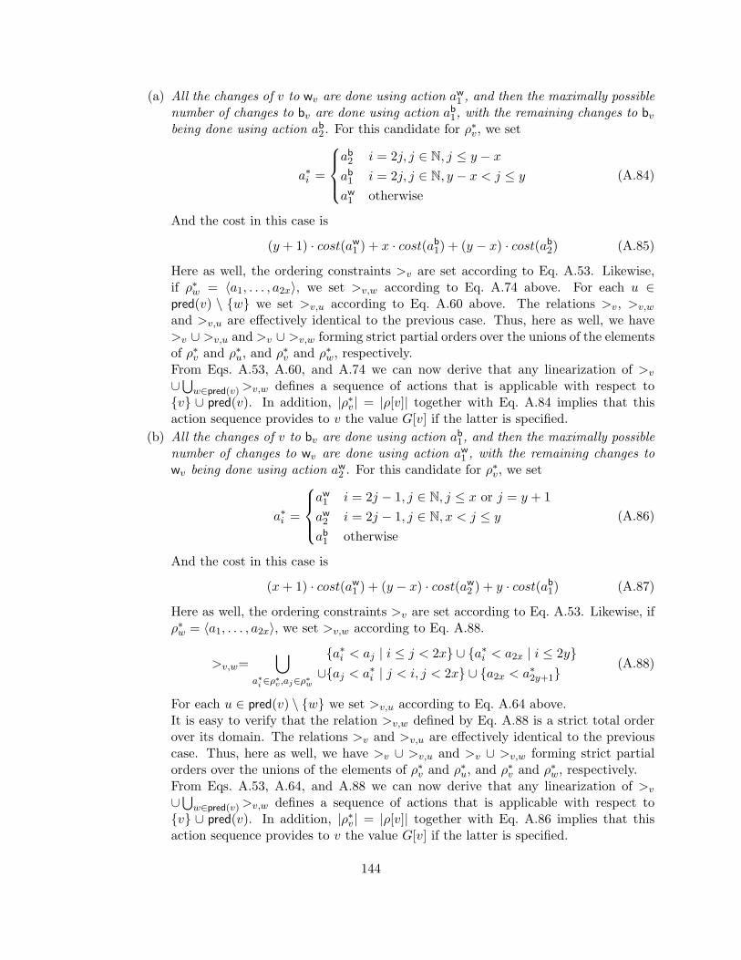
(a) All the changes of v to wv are done using action aw1 , and then the maximally possible
number of changes to bv are done using action ab1, with the remaining changes to bv
being done using action ab2. For this candidate for ρ∗v, we set
a∗i =
ab
2 i = 2j, j ∈ N, j ≤ y − xab
1 i = 2j, j ∈ N, y − x < j ≤ yaw
1 otherwise
(A.84)
And the cost in this case is
(y + 1) · cost(aw1 ) + x · cost(ab
1) + (y − x) · cost(ab2) (A.85)
Here as well, the ordering constraints >v are set according to Eq. A.53. Likewise,if ρ∗w = 〈a1, . . . , a2x〉, we set >v,w according to Eq. A.74 above. For each u ∈pred(v) \ {w} we set >v,u according to Eq. A.60 above. The relations >v, >v,wand >v,u are effectively identical to the previous case. Thus, here as well, we have>v ∪ >v,u and >v ∪ >v,w forming strict partial orders over the unions of the elementsof ρ∗v and ρ∗u, and ρ∗v and ρ∗w, respectively.From Eqs. A.53, A.60, and A.74 we can now derive that any linearization of >v∪⋃w∈pred(v)>v,w defines a sequence of actions that is applicable with respect to{v} ∪ pred(v). In addition, |ρ∗v| = |ρ[v]| together with Eq. A.84 implies that thisaction sequence provides to v the value G[v] if the latter is specified.
(b) All the changes of v to bv are done using action ab1, and then the maximally possible
number of changes to wv are done using action aw1 , with the remaining changes to
wv being done using action aw2 . For this candidate for ρ∗v, we set
a∗i =
aw
1 i = 2j − 1, j ∈ N, j ≤ x or j = y + 1aw
2 i = 2j − 1, j ∈ N, x < j ≤ yab
1 otherwise
(A.86)
And the cost in this case is
(x+ 1) · cost(aw1 ) + (y − x) · cost(aw
2 ) + y · cost(ab1) (A.87)
Here as well, the ordering constraints >v are set according to Eq. A.53. Likewise, ifρ∗w = 〈a1, . . . , a2x〉, we set >v,w according to Eq. A.88.
>v,w=⋃
a∗i∈ρ∗v ,aj∈ρ∗w
{a∗i < aj | i ≤ j < 2x} ∪ {a∗i < a2x | i ≤ 2y}∪{aj < a∗i | j < i, j < 2x} ∪ {a2x < a∗2y+1}
(A.88)
For each u ∈ pred(v) \ {w} we set >v,u according to Eq. A.64 above.It is easy to verify that the relation >v,w defined by Eq. A.88 is a strict total orderover its domain. The relations >v and >v,u are effectively identical to the previouscase. Thus, here as well, we have >v ∪ >v,u and >v ∪ >v,w forming strict partialorders over the unions of the elements of ρ∗v and ρ∗u, and ρ∗v and ρ∗w, respectively.From Eqs. A.53, A.64, and A.88 we can now derive that any linearization of >v∪⋃w∈pred(v)>v,w defines a sequence of actions that is applicable with respect to{v} ∪ pred(v). In addition, |ρ∗v| = |ρ[v]| together with Eq. A.86 implies that thisaction sequence provides to v the value G[v] if the latter is specified.
144
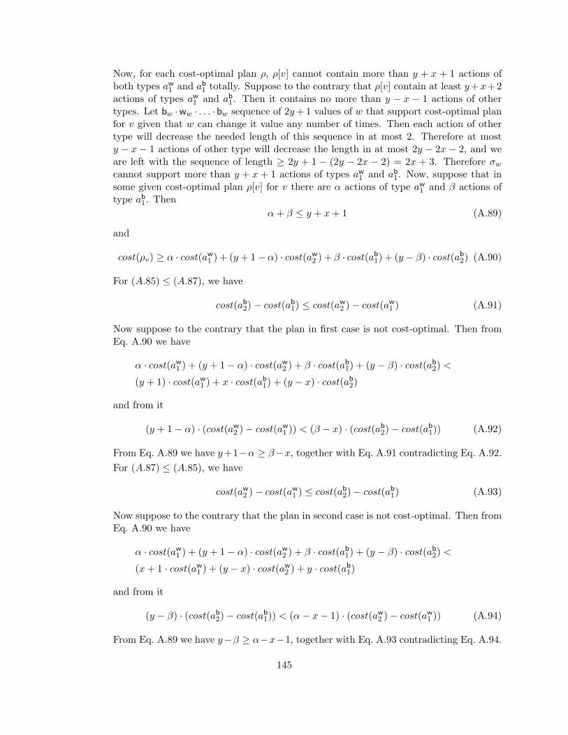
Now, for each cost-optimal plan ρ, ρ[v] cannot contain more than y + x + 1 actions ofboth types aw
1 and ab1 totally. Suppose to the contrary that ρ[v] contain at least y+x+2
actions of types aw1 and ab
1. Then it contains no more than y − x − 1 actions of othertypes. Let bw ·ww · . . . · bw sequence of 2y+ 1 values of w that support cost-optimal planfor v given that w can change it value any number of times. Then each action of othertype will decrease the needed length of this sequence in at most 2. Therefore at mosty − x − 1 actions of other type will decrease the length in at most 2y − 2x − 2, and weare left with the sequence of length ≥ 2y + 1 − (2y − 2x − 2) = 2x + 3. Therefore σwcannot support more than y + x + 1 actions of types aw
1 and ab1. Now, suppose that in
some given cost-optimal plan ρ[v] for v there are α actions of type aw1 and β actions of
type ab1. Then
α+ β ≤ y + x+ 1 (A.89)
and
cost(ρv) ≥ α · cost(aw1 ) + (y + 1− α) · cost(aw
2 ) + β · cost(ab1) + (y − β) · cost(ab
2) (A.90)
For (A.85) ≤ (A.87), we have
cost(ab2)− cost(ab
1) ≤ cost(aw2 )− cost(aw
1 ) (A.91)
Now suppose to the contrary that the plan in first case is not cost-optimal. Then fromEq. A.90 we have
α · cost(aw1 ) + (y + 1− α) · cost(aw
2 ) + β · cost(ab1) + (y − β) · cost(ab
2) <
(y + 1) · cost(aw1 ) + x · cost(ab
1) + (y − x) · cost(ab2)
and from it
(y + 1− α) · (cost(aw2 )− cost(aw
1 )) < (β − x) · (cost(ab2)− cost(ab
1)) (A.92)
From Eq. A.89 we have y+1−α ≥ β−x, together with Eq. A.91 contradicting Eq. A.92.For (A.87) ≤ (A.85), we have
cost(aw2 )− cost(aw
1 ) ≤ cost(ab2)− cost(ab
1) (A.93)
Now suppose to the contrary that the plan in second case is not cost-optimal. Then fromEq. A.90 we have
α · cost(aw1 ) + (y + 1− α) · cost(aw
2 ) + β · cost(ab1) + (y − β) · cost(ab
2) <
(x+ 1 · cost(aw1 ) + (y − x) · cost(aw
2 ) + y · cost(ab1)
and from it
(y − β) · (cost(ab2)− cost(ab
1)) < (α− x− 1) · (cost(aw2 )− cost(aw
1 )) (A.94)
From Eq. A.89 we have y−β ≥ α−x−1, together with Eq. A.93 contradicting Eq. A.94.
145
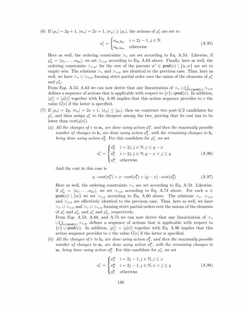
(6) If |ρv| = 2y + 1, |σw| = 2x+ 1, |σw| ≥ |ρv|, the actions of ρ∗v are set to
a∗i =
{awv |bw i = 2j − 1, j ∈ Nabv |ww otherwise
(A.95)
Here as well, the ordering constraints >v are set according to Eq. A.53. Likewise, ifρ∗w = 〈a1, . . . , a2x〉, we set >v,w according to Eq. A.63 above. Finally, here as well, theordering constraints >v,w′ for the rest of the parents w′ ∈ pred(v) \ {u,w} are set toempty sets. The relations >v and >v,w are identical to the previous case. Thus, here aswell, we have >v ∪ >v,w forming strict partial order over the union of the elements of ρ∗vand ρ∗w.From Eqs. A.53, A.63 we can now derive that any linearization of >v ∪
⋃w∈pred(v)>v,w
defines a sequence of actions that is applicable with respect to {v}∪pred(v). In addition,|ρ∗v| = |ρ[v]| together with Eq. A.95 implies that this action sequence provides to v thevalue G[v] if the latter is specified.
(7) If |ρv| = 2y, |σw| = 2x + 1, |σw| ≤ |ρv|, then we construct two post-3/2 candidates forρ∗v, and then assign ρ∗v to the cheapest among the two, proving that its cost has to belower than cost(ρ[v]).(a) All the changes of v to wv are done using action aw
1 , and then the maximally possiblenumber of changes to bv are done using action ab
1, with the remaining changes to bvbeing done using action ab
2. For this candidate for ρ∗v, we set
a∗i =
ab
2 i = 2j, j ∈ N, j ≤ y − xab
1 i = 2j, j ∈ N, y − x < j ≤ yaw
1 otherwise
(A.96)
And the cost in this case is
y · cost(aw1 ) + x · cost(ab
1) + (y − x) · cost(ab2) (A.97)
Here as well, the ordering constraints >v are set according to Eq. A.53. Likewise,if ρ∗w = 〈a1, . . . , a2x〉, we set >v,w according to Eq. A.74 above. For each u ∈pred(v) \ {w} we set >v,u according to Eq. A.60 above. The relations >v, >v,wand >v,u are effectively identical to the previous case. Thus, here as well, we have>v ∪ >v,u and >v ∪ >v,w forming strict partial orders over the unions of the elementsof ρ∗v and ρ∗u, and ρ∗v and ρ∗w, respectively.From Eqs. A.53, A.60, and A.74 we can now derive that any linearization of >v∪⋃w∈pred(v)>v,w defines a sequence of actions that is applicable with respect to{v} ∪ pred(v). In addition, |ρ∗v| = |ρ[v]| together with Eq. A.96 implies that thisaction sequence provides to v the value G[v] if the latter is specified.
(b) All the changes of v to bv are done using action ab1, and then the maximally possible
number of changes to wv are done using action aw1 , with the remaining changes to
wv being done using action aw2 . For this candidate for ρ∗v, we set
a∗i =
aw
1 i = 2j − 1, j ∈ N, j ≤ xaw
2 i = 2j − 1, j ∈ N, x < j ≤ yab
1 otherwise
(A.98)
146
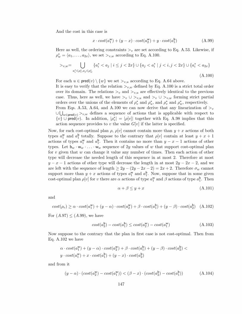
And the cost in this case is
x · cost(aw1 ) + (y − x) · cost(aw
2 ) + y · cost(ab1) (A.99)
Here as well, the ordering constraints >v are set according to Eq. A.53. Likewise, ifρ∗w = 〈a1, . . . , a2x〉, we set >v,w according to Eq. A.100.
>v,w=⋃
a∗i∈ρ∗v ,aj∈ρ∗w
{a∗i < aj | i ≤ j < 2x} ∪ {aj < a∗i | j < i, j < 2x} ∪ {a∗i < a2x}
(A.100)For each u ∈ pred(v) \ {w} we set >v,u according to Eq. A.64 above.It is easy to verify that the relation >v,w defined by Eq. A.100 is a strict total orderover its domain. The relations >v and >v,u are effectively identical to the previouscase. Thus, here as well, we have >v ∪ >v,u and >v ∪ >v,w forming strict partialorders over the unions of the elements of ρ∗v and ρ∗u, and ρ∗v and ρ∗w, respectively.From Eqs. A.53, A.64, and A.100 we can now derive that any linearization of >v∪⋃w∈pred(v)>v,w defines a sequence of actions that is applicable with respect to{v} ∪ pred(v). In addition, |ρ∗v| = |ρ[v]| together with Eq. A.98 implies that thisaction sequence provides to v the value G[v] if the latter is specified.
Now, for each cost-optimal plan ρ, ρ[v] cannot contain more than y + x actions of bothtypes aw
1 and ab1 totally. Suppose to the contrary that ρ[v] contain at least y + x + 1
actions of types aw1 and ab
1. Then it contains no more than y − x − 1 actions of othertypes. Let bw · ww · . . . · ww sequence of 2y values of w that support cost-optimal planfor v given that w can change it value any number of times. Then each action of othertype will decrease the needed length of this sequence in at most 2. Therefore at mosty − x − 1 actions of other type will decrease the length in at most 2y − 2x − 2, and weare left with the sequence of length ≥ 2y− (2y− 2x− 2) = 2x+ 2. Therefore σw cannotsupport more than y + x actions of types aw
1 and ab1. Now, suppose that in some given
cost-optimal plan ρ[v] for v there are α actions of type aw1 and β actions of type ab
1. Then
α+ β ≤ y + x (A.101)
and
cost(ρv) ≥ α · cost(aw1 ) + (y − α) · cost(aw
2 ) + β · cost(ab1) + (y − β) · cost(ab
2) (A.102)
For (A.97) ≤ (A.99), we have
cost(ab2)− cost(ab
1) ≤ cost(aw2 )− cost(aw
1 ) (A.103)
Now suppose to the contrary that the plan in first case is not cost-optimal. Then fromEq. A.102 we have
α · cost(aw1 ) + (y − α) · cost(aw
2 ) + β · cost(ab1) + (y − β) · cost(ab
2) <
y · cost(aw1 ) + x · cost(ab
1) + (y − x) · cost(ab2)
and from it
(y − α) · (cost(aw2 )− cost(aw
1 )) < (β − x) · (cost(ab2)− cost(ab
1)) (A.104)
147
From Eq. A.101 we have y−α ≥ β−x, together with Eq. A.103 contradicting Eq. A.104.For (A.99) ≤ (A.97), we have
cost(aw2 )− cost(aw
1 ) ≤ cost(ab2)− cost(ab
1) (A.105)
Now suppose to the contrary that the plan in second case is not cost-optimal. Then fromEq. A.102 we have
α · cost(aw1 ) + (y − α) · cost(aw
2 ) + β · cost(ab1) + (y − β) · cost(ab
2) <
x · cost(aw1 ) + (y − x) · cost(aw
2 ) + y · cost(ab1)
and from it
(y − β) · (cost(ab2)− cost(ab
1)) < (α− x) · (cost(aw2 )− cost(aw
1 )) (A.106)
From Eq. A.101 we have y−β ≥ α−x, together with Eq. A.105 contradicting Eq. A.106.
(8) If |ρv| = 2y, |σw| = 2x+ 1, |σw| > |ρv|, then the actions of ρ∗v are set to
a∗i =
{awv |bw i = 2j − 1, j ∈ Nabv |ww otherwise
(A.107)
Here as well, the ordering constraints >v are set according to Eq. A.53. Likewise, ifρ∗w = 〈a1, . . . , a2x〉, we set >v,w according to Eq. A.63 above. Finally, here as well, theordering constraints >v,w′ for the rest of the parents w′ ∈ pred(v) \ {u,w} are set toempty sets. The relations >v and >v,w are identical to the previous case. Thus, here aswell, we have >v ∪ >v,w forming strict partial order over the union of the elements of ρ∗vand ρ∗w.From Eqs. A.53, A.63 we can now derive that any linearization of >v ∪
⋃w∈pred(v)>v,w
defines a sequence of actions that is applicable with respect to {v}∪pred(v). In addition,|ρ∗v| = |ρ[v]| together with Eq. A.107 implies that this action sequence provides to v thevalue G[v] if the latter is specified.
(IV) If γ = ww, δ = bw, we distinguish between a few cases based on σw and σv.
(1) If |ρv| = 2y + 1, |σw| = 2x, |σw| ≤ |ρv|, then we construct two post-3/2 candidates forρ∗v, and then assign ρ∗v to the cheapest among the two, proving that its cost has to belower than cost(ρ[v]).
(a) All the changes of v to wv are done using action aw1 , and then the maximally possible
number of changes to bv are done using action ab1, with the remaining changes to bv
being done using action ab2. For this candidate for ρ∗v, we set
a∗i =
ab
2 i = 2j, j ∈ N, j ≤ y − x+ 1ab
1 i = 2j, j ∈ N, y − x+ 1 < j ≤ yaw
1 otherwise
(A.108)
And the cost in this case is
(y + 1) · cost(aw1 ) + (x− 1) · cost(ab
1) + (y − x+ 1) · cost(ab2) (A.109)
148
Here as well, the ordering constraints >v are set according to Eq. A.53. Likewise, ifρ∗w = 〈a1, . . . , a2x−1〉, we set >v,w according to Eq. A.110.
>v,w=⋃
a∗i∈ρ∗v ,aj∈ρ∗w
{a∗i < aj | i < j} ∪ {aj < a∗i | j ≤ i} (A.110)
For each u ∈ pred(v) \ {w} we set >v,u according to Eq. A.60.It is easy to verify that the relation >v,w defined by Eq. A.110 is a strict total orderover its domain. The relations >v and >v,u are effectively identical to the previouscase. Thus, here as well, we have >v ∪ >v,u and >v ∪ >v,w forming strict partialorders over the unions of the elements of ρ∗v and ρ∗u, and ρ∗v and ρ∗w, respectively.From Eqs. A.53, A.60, and A.110 we can now derive that any linearization of >v∪⋃w∈pred(v)>v,w defines a sequence of actions that is applicable with respect to{v} ∪ pred(v). In addition, |ρ∗v| = |ρ[v]| together with Eq. A.108 implies that thisaction sequence provides to v the value G[v] if the latter is specified.
(b) All the changes of v to bv are done using action ab1, and then the maximally possible
number of changes to wv are done using action aw1 , with the remaining changes to
wv being done using action aw2 . For this candidate for ρ∗v, we set
a∗i =
aw
2 i = 2j − 1, j ∈ N, j ≤ y − x+ 1aw
1 i = 2j − 1, j ∈ N, y − x+ 1 < j ≤ y + 1ab
1 otherwise
(A.111)
And the cost in this case is
x · cost(aw1 ) + (y + 1− x) · cost(aw
2 ) + y · cost(ab1) (A.112)
Here as well, the ordering constraints >v are set according to Eq. A.53. Likewise, ifρ∗w = 〈a1, . . . , a2x−1〉, we set >v,w according to Eq. A.113.
>v,w=⋃
a∗i∈ρ∗v ,aj∈ρ∗w
{a∗i < aj | i ≤ 2y − 2x+ 1 + j} ∪ {aj < a∗i | i > 2y − 2x+ 1 + j}
(A.113)For each u ∈ pred(v) \ {w} we set >v,u according to Eq. A.64.It is easy to verify that the relation >v,w defined by Eq. A.113 is a strict total orderover its domain. The relations >v and >v,u are effectively identical to the previouscase. Thus, here as well, we have >v ∪ >v,u and >v ∪ >v,w forming strict partialorders over the unions of the elements of ρ∗v and ρ∗u, and ρ∗v and ρ∗w, respectively.From Eqs. A.53, A.64, and A.113 we can now derive that any linearization of >v∪⋃w∈pred(v)>v,w defines a sequence of actions that is applicable with respect to{v} ∪ pred(v). In addition, |ρ∗v| = |ρ[v]| together with Eq. A.111 implies that thisaction sequence provides to v the value G[v] if the latter is specified.
Now, for each cost-optimal plan ρ, ρ[v] cannot contain more than y + x actions of bothtypes aw
1 and ab1 totally. Suppose to the contrary that ρ[v] contain at least y + x + 1
actions of types aw1 and ab
1. Then it contains no more than y − x actions of other types.Let ww · wb · . . . · ww sequence of 2y + 1 values of w that support cost-optimal plan for v
149
given that w can change it value any number of times. Then each action of other typewill decrease the needed length of this sequence in at most 2. Therefore at most y − xactions of other type will decrease the length in at most 2y − 2x, and we are left withthe sequence of length ≥ 2y+ 1− (2y−2x) = 2x+ 1. Therefore σw cannot support morethan y + x actions of types aw
1 and ab1. Now, suppose that in some given cost-optimal
plan ρ[v] for v there are α actions of type aw1 and β actions of type ab
1. Then
α+ β ≤ y + x (A.114)
and
cost(ρv) ≥ α · cost(aw1 ) + (y+ 1−α) · cost(aw
2 ) + β · cost(ab1) + (y− β) · cost(ab
2) (A.115)
For (A.109) ≤ (A.112), we have
cost(ab2)− cost(ab
1) ≤ cost(aw2 )− cost(aw
1 ) (A.116)
Now suppose to the contrary that the plan in first case is not cost-optimal. Then fromEq. A.115 we have
α · cost(aw1 ) + (y + 1− α) · cost(aw
2 ) + β · cost(ab1) + (y − β) · cost(ab
2) <
(y + 1) · cost(aw1 ) + (x− 1) · cost(ab
1) + (y − x+ 1) · cost(ab2)
and from it
(y + 1− α) · (cost(aw2 )− cost(aw
1 )) < (β − x+ 1) · (cost(ab2)− cost(ab
1)) (A.117)
From Eq. A.114 we have y + 1 − α ≥ β − x + 1, together with Eq. A.116 contradictingEq. A.117.For (A.112) ≤ (A.109), we have
cost(aw2 )− cost(aw
1 ) ≤ cost(ab2)− cost(ab
1) (A.118)
Now suppose to the contrary that the plan in second case is not cost-optimal. Then fromEq. A.115 we have
α · cost(aw1 ) + (y + 1− α) · cost(aw
2 ) + β · cost(ab1) + (y − β) · cost(ab
2) <
x · cost(aw1 ) + (y − x+ 1) · cost(aw
2 ) + y · cost(ab1)
and from it
(y − β) · (cost(ab2)− cost(ab
1)) < (α− x) · (cost(aw2 )− cost(aw
1 )) (A.119)
From Eq. A.114 we have y−β ≥ α−x, together with Eq. A.118 contradicting Eq. A.119.
(2) If |ρv| = 2y + 1, |σw| = 2x, |σw| > |ρv|, then the actions of ρ∗v are set to
a∗i =
{awv |ww i = 2j − 1, j ∈ Nabv |bw otherwise
(A.120)
150
Here as well, the ordering constraints >v are set according to Eq. A.53. Likewise, ifρ∗w = 〈a1, . . . , a2x−1〉, we set >v,w according to Eq. A.110 above.Finally, here as well, the ordering constraints >v,w′ for the rest of the parents w′ ∈pred(v) \ {u,w} are set to empty sets.The relations >v and >v,w are identical to the previous case. Thus, here as well, we have>v ∪ >v,w forming strict partial order over the union of the elements of ρ∗v and ρ∗w.From Eqs. A.53, A.110 we can now derive that any linearization of >v ∪
⋃w∈pred(v)>v,w
defines a sequence of actions that is applicable with respect to {v}∪pred(v). In addition,|ρ∗v| = |ρ[v]| together with Eq. A.120 implies that this action sequence provides to v thevalue G[v] if the latter is specified.
(3) If |ρv| = 2y, |σw| = 2x, |σw| ≤ |ρv| + 1, then we construct two post-3/2 candidates forρ∗v, and then assign ρ∗v to the cheapest among the two, proving that its cost has to belower than cost(ρ[v]).
(a) All the changes of v to wv are done using action aw1 , and then the maximally possible
number of changes to bv are done using action ab1, with the remaining changes to bv
being done using action ab2. For this candidate for ρ∗v, we set
a∗i =
ab
1 i = 2j, j ∈ N, j < x
ab2 i = 2j, j ∈ N, x ≤ j ≤ yaw
1 otherwise
(A.121)
And the cost in this case is
y · cost(aw1 ) + (x− 1) · cost(ab
1) + (y − x+ 1) · cost(ab2) (A.122)
Here as well, the ordering constraints >v are set according to Eq. A.53. Likewise, ifρ∗w = 〈a1, . . . , a2x−1〉, we set >v,w according to Eq. A.110 above.For each u ∈ pred(v) \ {w} we set >v,u according to Eq. A.60.The relations >v, >v,w and >v,u are effectively identical to the previous case. Thus,here as well, we have >v ∪ >v,u and >v ∪ >v,w forming strict partial orders over theunions of the elements of ρ∗v and ρ∗u, and ρ∗v and ρ∗w, respectively.From Eqs. A.53, A.60, and A.110 we can now derive that any linearization of >v∪⋃w∈pred(v)>v,w defines a sequence of actions that is applicable with respect to{v} ∪ pred(v). In addition, |ρ∗v| = |ρ[v]| together with Eq. A.121 implies that thisaction sequence provides to v the value G[v] if the latter is specified.
(b) All the changes of v to bv are done using action ab1, and then the maximally possible
number of changes to wv are done using action aw1 , with the remaining changes to
wv being done using action aw2 . For this candidate for ρ∗v, we set
a∗i =
aw
2 i = 2j − 1, j ∈ N, j ≤ y − x+ 1aw
1 i = 2j − 1, j ∈ N, y − x+ 1 < j ≤ yab
1 otherwise
(A.123)
And the cost in this case is
(x− 1) · cost(aw1 ) + (y − x+ 1) · cost(aw
2 ) + y · cost(ab1) (A.124)
151
Here as well, the ordering constraints >v are set according to Eq. A.53. Likewise, ifρ∗w = 〈a1, . . . , a2x−1〉, we set >v,w according to Eq. A.113 above.For each u ∈ pred(v) \ {w} we set >v,u according to Eq. A.64.The relations >v, >v,w and >v,u are effectively identical to the previous case. Thus,here as well, we have >v ∪ >v,u and >v ∪ >v,w forming strict partial orders over theunions of the elements of ρ∗v and ρ∗u, and ρ∗v and ρ∗w, respectively.From Eqs. A.53, A.64, and A.113 we can now derive that any linearization of >v∪⋃w∈pred(v)>v,w defines a sequence of actions that is applicable with respect to{v} ∪ pred(v). In addition, |ρ∗v| = |ρ[v]| together with Eq. A.123 implies that thisaction sequence provides to v the value G[v] if the latter is specified.
Now, for each cost-optimal plan ρ, ρ[v] cannot contain more than y+x−1 actions of bothtypes aw
1 and ab1 totally. Suppose to the contrary that ρ[v] contain at least y+ x actions
of types aw1 and ab
1. Then it contains no more than y − x actions of other types. Letww ·bw · . . . ·bw sequence of 2y values of w that support cost-optimal plan for v given thatw can change it value any number of times. Then each action of other type will decreasethe needed length of this sequence in at most 2. Therefore at most y − x actions ofother type will decrease the length in at most 2y− 2x, and we are left with the sequenceof length ≥ 2y − (2y − 2x) = 2x, which have to be a subsequence of σw, contradictingwith the fact that σw is of the same or smaller size and starts with a different character.Therefore σw cannot support more than y+x actions of types aw
1 and ab1. Now, suppose
that in some given cost-optimal plan ρ[v] for v there are α actions of type aw1 and β
actions of type ab1. Then
α+ β ≤ y + x (A.125)
and
cost(ρv) ≥ α · cost(aw1 ) + (y − α) · cost(aw
2 ) + β · cost(ab1) + (y − β) · cost(ab
2) (A.126)
For (A.122) ≤ (A.124), we have
cost(ab2)− cost(ab
1) ≤ cost(aw2 )− cost(aw
1 ) (A.127)
Now suppose to the contrary that the plan in first case is not cost-optimal. Then fromEq. A.126 we have
α · cost(aw1 ) + (y − α) · cost(aw
2 ) + β · cost(ab1) + (y − β) · cost(ab
2) <
y · cost(aw1 ) + x · cost(ab
1) + (y − x) · cost(ab2)
and from it
(y − α) · (cost(aw2 )− cost(aw
1 )) < (β − x) · (cost(ab2)− cost(ab
1)) (A.128)
From Eq. A.125 we have y−α ≥ β−x, together with Eq. A.127 contradicting Eq. A.128.For (A.124) ≤ (A.122), we have
cost(aw2 )− cost(aw
1 ) ≤ cost(ab2)− cost(ab
1) (A.129)
152
Now suppose to the contrary that the plan in second case is not cost-optimal. Then fromEq. A.126 we have
α · cost(aw1 ) + (y − α) · cost(aw
2 ) + β · cost(ab1) + (y − β) · cost(ab
2) <
x · cost(aw1 ) + (y − x) · cost(aw
2 ) + y · cost(ab1)
and from it
(y − β) · (cost(ab2)− cost(ab
1)) < (α− x) · (cost(aw2 )− cost(aw
1 )) (A.130)
From Eq. A.125 we have y−β ≥ α−x, together with Eq. A.129 contradicting Eq. A.130.
(4) If |ρv| = 2y, |σw| = 2x, |σw| > |ρv|+ 1, then the actions of ρ∗v are set to
a∗i =
{awv |ww i = 2j − 1, j ∈ Nabv |bw otherwise
(A.131)
Here as well, the ordering constraints >v are set according to Eq. A.53. Likewise, ifρ∗w = 〈a1, . . . , a2x−1〉, we set >v,w according to Eq. A.110 above.Finally, here as well, the ordering constraints >v,w′ for the rest of the parents w′ ∈pred(v) \ {u,w} are set to empty sets.The relations >v and >v,w are identical to the previous case. Thus, here as well, we have>v ∪ >v,w forming strict partial order over the union of the elements of ρ∗v and ρ∗w.From Eqs. A.53, A.110 we can now derive that any linearization of >v ∪
⋃w∈pred(v)>v,w
defines a sequence of actions that is applicable with respect to {v}∪pred(v). In addition,|ρ∗v| = |ρ[v]| together with Eq. A.131 implies that this action sequence provides to v thevalue G[v] if the latter is specified.
(5) If |ρv| = 2y+1, |σw| = 2x+1, |σw| ≤ |ρv|+1, then we construct two post-3/2 candidatesfor ρ∗v, and then assign ρ∗v to the cheapest among the two, proving that its cost has tobe lower than cost(ρ[v]).
(a) All the changes of v to wv are done using action aw1 , and then the maximally possible
number of changes to bv are done using action ab1, with the remaining changes to bv
being done using action ab2. For this candidate for ρ∗v, we set
a∗i =
ab
1 i = 2j, j ∈ N, j < x
ab2 i = 2j, j ∈ N, x ≤ j ≤ yaw
1 otherwise
(A.132)
And the cost in this case is
(y + 1) · cost(aw1 ) + (x− 1) · cost(ab
1) + (y − x+ 1) · cost(ab2) (A.133)
Here as well, the ordering constraints >v are set according to Eq. A.53. Likewise, ifρ∗w = 〈a1, . . . , a2x〉, we set >v,w according to Eq. A.134.
>v,w=⋃
a∗i∈ρ∗v ,aj∈ρ∗w
{a∗i < aj | i < j < 2x} ∪ {aj < a∗i | j ≤ i, j < 2x} ∪ {a∗i < a2x}
(A.134)
153
For each u ∈ pred(v) \ {w} we set >v,u according to Eq. A.60.It is easy to verify that the relation >v,w defined by Eq. A.134 is a strict total orderover its domain. The relations >v and >v,u are effectively identical to the previouscase. Thus, here as well, we have >v ∪ >v,u and >v ∪ >v,w forming strict partialorders over the unions of the elements of ρ∗v and ρ∗u, and ρ∗v and ρ∗w, respectively.From Eqs. A.53, A.60, and A.134 we can now derive that any linearization of >v∪⋃w∈pred(v)>v,w defines a sequence of actions that is applicable with respect to{v} ∪ pred(v). In addition, |ρ∗v| = |ρ[v]| together with Eq. A.132 implies that thisaction sequence provides to v the value G[v] if the latter is specified.
(b) All the changes of v to bv are done using action ab1, and then the maximally possible
number of changes to wv are done using action aw1 , with the remaining changes to
wv being done using action aw2 . For this candidate for ρ∗v, we set
a∗i =
aw
2 i = 2j − 1, j ∈ N, j ≤ y − x or j = y + 1aw
1 i = 2j − 1, j ∈ N, y − x < j ≤ yab
1 otherwise
(A.135)
And the cost in this case is
x · cost(aw1 ) + (y + 1− x) · cost(aw
2 ) + y · cost(ab1) (A.136)
Here as well, the ordering constraints >v are set according to Eq. A.53. Likewise, ifρ∗w = 〈a1, . . . , a2x−1〉, we set >v,w according to Eq. A.137.
>v,w=⋃
a∗i∈ρ∗v ,aj∈ρ∗w
{a∗i < aj | i < 2y − 2x+ j} ∪ {aj < a∗i | i ≥ 2y − 2x+ j}
(A.137)For each u ∈ pred(v) \ {w} we set >v,u according to Eq. A.64.It is easy to verify that the relation >v,w defined by Eq. A.137 is a strict total orderover its domain. The relations >v and >v,u are effectively identical to the previouscase. Thus, here as well, we have >v ∪ >v,u and >v ∪ >v,w forming strict partialorders over the unions of the elements of ρ∗v and ρ∗u, and ρ∗v and ρ∗w, respectively.From Eqs. A.53, A.64, and A.137 we can now derive that any linearization of >v∪⋃w∈pred(v)>v,w defines a sequence of actions that is applicable with respect to{v} ∪ pred(v). In addition, |ρ∗v| = |ρ[v]| together with Eq. A.135 implies that thisaction sequence provides to v the value G[v] if the latter is specified.
Now, for each cost-optimal plan ρ, ρ[v] cannot contain more than y + x + 1 actions ofboth types aw
1 and ab1 totally. Suppose to the contrary that ρ[v] contain at least y+x+2
actions of types aw1 and ab
1. Then it contains no more than y − x − 1 actions of othertypes. Let ww ·bw · . . . ·ww sequence of 2y+ 1 values of w that support cost-optimal planfor v given that w can change it value any number of times. Then each action of othertype will decrease the needed length of this sequence in at most 2. Therefore at mosty − x − 1 actions of other type will decrease the length in at most 2y − 2x − 2, and weare left with the sequence of length ≥ 2y + 1 − (2y − 2x − 2) = 2x + 3. Therefore σwcannot support more than y + x + 1 actions of types aw
1 and ab1. Now, suppose that in
154
some given cost-optimal plan ρ[v] for v there are α actions of type aw1 and β actions of
type ab1. Then
α+ β ≤ y + x+ 1 (A.138)
and
cost(ρv) ≥ α · cost(aw1 ) + (y+ 1−α) · cost(aw
2 ) + β · cost(ab1) + (y− β) · cost(ab
2) (A.139)
For (A.133) ≤ (A.136), we have
cost(ab2)− cost(ab
1) ≤ cost(aw2 )− cost(aw
1 ) (A.140)
Now suppose to the contrary that the plan in first case is not cost-optimal. Then fromEq. A.139 we have
α · cost(aw1 ) + (y + 1− α) · cost(aw
2 ) + β · cost(ab1) + (y − β) · cost(ab
2) <
(y + 1) · cost(aw1 ) + x · cost(ab
1) + (y − x) · cost(ab2)
and from it
(y + 1− α) · (cost(aw2 )− cost(aw
1 )) < (β − x) · (cost(ab2)− cost(ab
1)) (A.141)
From Eq. A.138 we have y + 1 − α ≥ β − x, together with Eq. A.140 contradictingEq. A.141.For (A.136) ≤ (A.133), we have
cost(aw2 )− cost(aw
1 ) ≤ cost(ab2)− cost(ab
1) (A.142)
Now suppose to the contrary that the plan in second case is not cost-optimal. Then fromEq. A.139 we have
α · cost(aw1 ) + (y + 1− α) · cost(aw
2 ) + β · cost(ab1) + (y − β) · cost(ab
2) <
(x+ 1 · cost(aw1 ) + (y − x) · cost(aw
2 ) + y · cost(ab1)
and from it
(y − β) · (cost(ab2)− cost(ab
1)) < (α− x− 1) · (cost(aw2 )− cost(aw
1 )) (A.143)
From Eq. A.138 we have y − β ≥ α − x − 1, together with Eq. A.142 contradictingEq. A.143.
(6) If |ρv| = 2y + 1, |σw| = 2x+ 1, |σw| > |ρv|+ 1, then the actions of ρ∗v are set to
a∗i =
{awv |ww i = 2j − 1, j ∈ Nabv |bw otherwise
(A.144)
Here as well, the ordering constraints >v are set according to Eq. A.53. Likewise, ifρ∗w = 〈a1, . . . , a2x−1〉, we set >v,w according to Eq. A.110 above.Finally, here as well, the ordering constraints >v,w′ for the rest of the parents w′ ∈pred(v) \ {u,w} are set to empty sets.
155
The relations >v and >v,w are identical to the previous case. Thus, here as well, we have>v ∪ >v,w forming strict partial order over the union of the elements of ρ∗v and ρ∗w.From Eqs. A.53, A.110 we can now derive that any linearization of >v ∪
⋃w∈pred(v)>v,w
defines a sequence of actions that is applicable with respect to {v}∪pred(v). In addition,|ρ∗v| = |ρ[v]| together with Eq. A.144 implies that this action sequence provides to v thevalue G[v] if the latter is specified.
(7) If |ρv| = 2y, |σw| = 2x + 1, |σw| ≤ |ρv|, then we construct two post-3/2 candidates forρ∗v, and then assign ρ∗v to the cheapest among the two, proving that its cost has to belower than cost(ρ[v]).
(a) All the changes of v to wv are done using action aw1 , and then the maximally possible
number of changes to bv are done using action ab1, with the remaining changes to bv
being done using action ab2. For this candidate for ρ∗v, we set
a∗i =
ab
2 i = 2j, j ∈ N, j ≤ y − xab
1 i = 2j, j ∈ N, y − x < j ≤ yaw
1 otherwise
(A.145)
And the cost in this case is
y · cost(aw1 ) + x · cost(ab
1) + (y − x) · cost(ab2) (A.146)
Here as well, the ordering constraints >v are set according to Eq. A.53. Likewise, ifρ∗w = 〈a1, . . . , a2x〉, we set >v,w according to Eq. A.147.
>v,w=[
a∗i ∈ρ∗v,aj∈ρ∗w
{a∗i < aj | i < 2y − 2x+ j, j > 1} ∪ {aj < a∗i | i ≥ 2y − 2x+ j} ∪ {a1 < a∗i }
(A.147)
For each u ∈ pred(v) \ {w} we set >v,u according to Eq. A.60.It is easy to verify that the relation >v,w defined by Eq. A.147 is a strict total orderover its domain. The relations >v and >v,u are effectively identical to the previouscase. Thus, here as well, we have >v ∪ >v,u and >v ∪ >v,w forming strict partialorders over the unions of the elements of ρ∗v and ρ∗u, and ρ∗v and ρ∗w, respectively.From Eqs. A.53, A.60, and A.147 we can now derive that any linearization of >v∪⋃w∈pred(v)>v,w defines a sequence of actions that is applicable with respect to{v} ∪ pred(v). In addition, |ρ∗v| = |ρ[v]| together with Eq. A.145 implies that thisaction sequence provides to v the value G[v] if the latter is specified.
(b) All the changes of v to bv are done using action ab1, and then the maximally possible
number of changes to wv are done using action aw1 , with the remaining changes to
wv being done using action aw2 . For this candidate for ρ∗v, we set
a∗i =
aw
2 i = 2j − 1, j ∈ N, j ≤ y − xaw
1 i = 2j − 1, j ∈ N, y − x < j ≤ yab
1 otherwise
(A.148)
And the cost in this case is
x · cost(aw1 ) + (y − x) · cost(aw
2 ) + y · cost(ab1) (A.149)
156
Here as well, the ordering constraints >v are set according to Eq. A.53. Likewise, ifρ∗w = 〈a1, . . . , a2x−1〉, we set >v,w according to Eq. A.137 above.For each u ∈ pred(v) \ {w} we set >v,u according to Eq. A.64 above.The relations >v, >v,w and >v,u are effectively identical to the previous case. Thus,here as well, we have >v ∪ >v,u and >v ∪ >v,w forming strict partial orders over theunions of the elements of ρ∗v and ρ∗u, and ρ∗v and ρ∗w, respectively.From Eqs. A.53, A.64, and A.137 we can now derive that any linearization of >v∪⋃w∈pred(v)>v,w defines a sequence of actions that is applicable with respect to{v} ∪ pred(v). In addition, |ρ∗v| = |ρ[v]| together with Eq. A.148 implies that thisaction sequence provides to v the value G[v] if the latter is specified.
Now, for each cost-optimal plan ρ, ρ[v] cannot contain more than y + x actions of bothtypes aw
1 and ab1 totally. Suppose to the contrary that ρ[v] contain at least y + x + 1
actions of types aw1 and ab
1. Then it contains no more than y − x − 1 actions of othertypes. Let ww · bw · . . . · bw sequence of 2y values of w that support cost-optimal plan forv given that w can change it value any number of times. Then each action of other typewill decrease the needed length of this sequence in at most 2. Therefore at most y−x−1actions of other type will decrease the length in at most 2y−2x−2, and we are left withthe sequence of length ≥ 2y− (2y−2x−2) = 2x+ 2. Therefore σw cannot support morethan y + x actions of types aw
1 and ab1. Now, suppose that in some given cost-optimal
plan ρ[v] for v there are α actions of type aw1 and β actions of type ab
1. Then
α+ β ≤ y + x (A.150)
and
cost(ρv) ≥ α · cost(aw1 ) + (y − α) · cost(aw
2 ) + β · cost(ab1) + (y − β) · cost(ab
2) (A.151)
For (A.146) ≤ (A.149), we have
cost(ab2)− cost(ab
1) ≤ cost(aw2 )− cost(aw
1 ) (A.152)
Now suppose to the contrary that the plan in first case is not cost-optimal. Then fromEq. A.151 we have
α · cost(aw1 ) + (y − α) · cost(aw
2 ) + β · cost(ab1) + (y − β) · cost(ab
2) <
y · cost(aw1 ) + x · cost(ab
1) + (y − x) · cost(ab2)
and from it
(y − α) · (cost(aw2 )− cost(aw
1 )) < (β − x) · (cost(ab2)− cost(ab
1)) (A.153)
From Eq. A.150 we have y−α ≥ β−x, together with Eq. A.152 contradicting Eq. A.153.For (A.149) ≤ (A.146), we have
cost(aw2 )− cost(aw
1 ) ≤ cost(ab2)− cost(ab
1) (A.154)
Now suppose to the contrary that the plan in second case is not cost-optimal. Then fromEq. A.151 we have
α · cost(aw1 ) + (y − α) · cost(aw
2 ) + β · cost(ab1) + (y − β) · cost(ab
2) <
x · cost(aw1 ) + (y − x) · cost(aw
2 ) + y · cost(ab1)
157
and from it
(y − β) · (cost(ab2)− cost(ab
1)) < (α− x) · (cost(aw2 )− cost(aw
1 )) (A.155)
From Eq. A.150 we have y−β ≥ α−x, together with Eq. A.154 contradicting Eq. A.155.
(8) If |ρv| = 2y, |σw| = 2x+ 1, |σw| > |ρv|, then the actions of ρ∗v are set to
a∗i =
{awv |ww i = 2j − 1, j ∈ Nabv |bw otherwise
(A.156)
Here as well, the ordering constraints >v are set according to Eq. A.53. Likewise, ifρ∗w = 〈a1, . . . , a2x−1〉, we set >v,w according to Eq. A.110 above.Finally, here as well, the ordering constraints >v,w′ for the rest of the parents w′ ∈pred(v) \ {u,w} are set to empty sets.The relations >v and >v,w are identical to the previous case. Thus, here as well, we have>v ∪ >v,w forming strict partial order over the union of the elements of ρ∗v and ρ∗w.
Until now, we have specified the sequences ρ∗v, the orders >v induced by these sequences, the orders>v,w, and proved that all >v ∪ >v,w and >w ∪ >v,w form strict partial orders over their domains.This construction allows us to apply now Theorem 22 to the (considered as sets) sequences ρ∗v andorders >v and >v,w, proving that
>=⋃v∈V
(>v ∪⋃
w∈pred(v)
>v,w)
forms a strict partial order over the union of ρ∗v1, . . . , ρ∗vn . Putting thing together, the above implies
that any linearization ρ∗ of > is a plan for Π, and post-3/2ness of all its subsequences ρ∗v1, . . . , ρ∗vn
then implies ρ∗ ∈ P3/2(Π). Moreover, if ρ is an optimal plan for Π, then cost(ρ∗) = cost(ρ) impliesthe optimality of ρ∗.
A.3.2 Construction
Given a post-3/2 action sequence % from A and a variable v ∈ V , we can distinguish between thefollowing exhaustive roles of each parent w ∈ pred(v) with respect to v along %.
R1 All the actions in % that change the value of v are supported by the same value of w.That is, for some γ ∈ {bw,ww}, if a ∈ %v, then a ∈ {abv |γ , awv |γ}.
R2 All the actions in % that change the value of v to wv are supported by the same value of w, andall the actions in % that change the value of v to bv are supported by another value of w.That is, for some γ 6= δ ∈ {bw,ww}, if a ∈ %v, then a ∈ {abv |γ , awv |δ}.
R3 All the actions in % that change the value of v to wv are supported by the same value of w, andnone of the actions in % that change the value of v to bv are supported by w.That is, for some γ ∈ {bw,ww} and δ 6∈ {bw,ww}, if a ∈ %v, then a ∈ {abv |δ, awv |γ}.
R4 All the actions in % that change the value of v to bv are supported by the same value of w, andnone of the actions in % that change the value of v to wv are supported by w.That is, for some γ ∈ {bw,ww} and δ 6∈ {bw,ww}, if a ∈ %v, then a ∈ {abv |γ , awv |δ}.
158
R5 All the actions in % that change the value of v to wv are supported by the same value of w, andall the actions in % that change the value of v to bv are supported by two values of w.That is, for some γ 6= δ ∈ {bw,ww}, if a ∈ %v, then a ∈ {awv |γ , abv |δ, abv |γ}.
R6 All the actions in % that change the value of v to bv are supported by the same value of w, andall the actions in % that change the value of v to wv are supported by two values of w.That is, for some γ 6= δ ∈ {bw,ww}, if a ∈ %v, then a ∈ {abv |γ , awv |δ, awv |γ}.
R7 All the actions in % that change the value of v to wv are supported by the same value of w, andsome of the actions in % that change the value of v to bv are supported by another value of wand others are supported by another parent.That is, for some γ 6= δ ∈ {bw,ww} and µ 6∈ {bw,ww}, if a ∈ %v, then a ∈ {awv |γ , abv |δ, abv |µ}.
R8 All the actions in % that change the value of v to bv are supported by the same value of w, andsome of the actions in % that change the value of v to wv are supported by another value of wand others are supported by another parent.That is, for some γ 6= δ ∈ {bw,ww} and µ 6∈ {bw,ww}, if a ∈ %v, then a ∈ {abv |γ , awv |δ, awv |µ}.
R9 Part of the actions in % that change the value of v to bv are supported by the same value of w,and none of the actions in % that change the value of v to wv are supported by the same valueof w.
R10 Part of the actions in % that change the value of v to wv are supported by the same value of w,and none of the actions in % that change the value of v to bv are supported by the same valueof w.
R11 None of the actions in % are supported by w.That is, if aα|γ ∈ %, then γ 6∈ {bw,ww}.
For a given post-3/2 action sequence % from A and a variable v ∈ V , each parent of v performsone of the roles R1-R11 with respect to v along %, and each of the roles R1-R10 is performed byat most one of the parents of v. In addition, there are sets of roles that cannot be simultaneouslyperformed by the parents of v with respect to v and the same action sequence %, and there are rolesthat have to be performed in pairs. Specifically,
• If one of the roles {R1,R2,R5,R6} is played by some parent w′ ∈ pred(v), then R11 must beplayed by all other parents w ∈ pred(v) \ {w′}.
• If R3/R7/R8 is played by some parent w1 ∈ pred(v), then R4/R9/R10, respectively, mustbe played by some parent w2 ∈ pred(v) \ {w1}, and R11 must be played by all other parentsw ∈ pred(v) \ {w1, w2}.
Considering a variable v and its parents pred(v) through the lens of these eleven roles, supposewe now aim at assigning these roles to pred(v) by considering them one after another in somearbitrary order. Given the aforementioned constraints on the role assignment, at each step of thissequential process we can be in one of the following eight states, with the whole process beingdescribed by a state machine depicted in Fig. A.6.
S1 All the roles R1-R11 are still available (to be assigned to the parents of v).
159
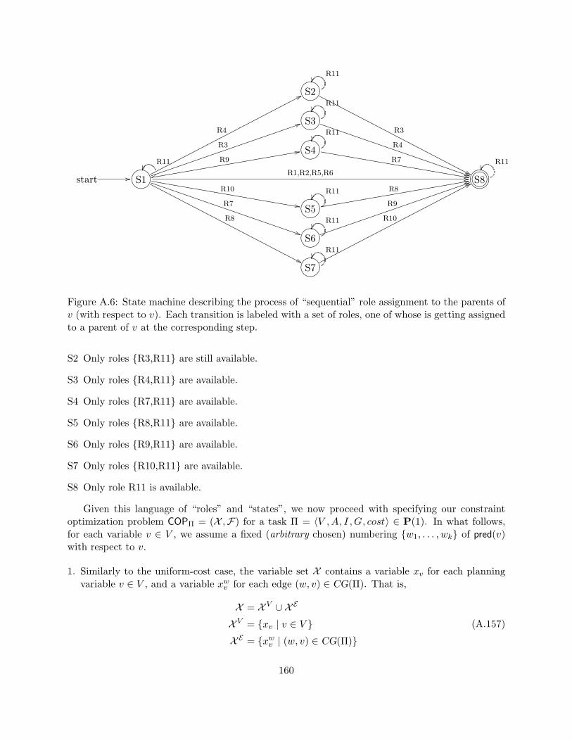
GFED@ABCS2
R3
''NNNNNNNNNNNNNNNNNNNNNNNNNNNNNNNNNNNNN
R11
GFED@ABCS3
R4
))TTTTTTTTTTTTTTTTTTTTTTTTTTTTTTTTTT
R11
GFED@ABCS4R7
,,YYYYYYYYYYYYYYYYYYYYYYYYYYYYYYYYY
R11
start // GFED@ABCS1R1,R2,R5,R6 //
R9
22eeeeeeeeeeeeeeeeeeeeeeeeeeeeeeeee
R3
55jjjjjjjjjjjjjjjjjjjjjjjjjjjjjjjjjj
R4
77ppppppppppppppppppppppppppppppppppppp
R10
,,YYYYYYYYYYYYYYYYYYYYYYYYYYYYYYYYY
R7
))TTTTTTTTTTTTTTTTTTTTTTTTTTTTTTTTTT
R8
''NNNNNNNNNNNNNNNNNNNNNNNNNNNNNNNNNNNNN
R11 GFED@ABC?>=<89:;S8
R11
GFED@ABCS5
R8
22eeeeeeeeeeeeeeeeeeeeeeeeeeeeeeeee
R11
GFED@ABCS6
R9
55jjjjjjjjjjjjjjjjjjjjjjjjjjjjjjjjjjR11
GFED@ABCS7
R10
77pppppppppppppppppppppppppppppppppppppR11
Figure A.6: State machine describing the process of “sequential” role assignment to the parents ofv (with respect to v). Each transition is labeled with a set of roles, one of whose is getting assignedto a parent of v at the corresponding step.
S2 Only roles {R3,R11} are still available.
S3 Only roles {R4,R11} are available.
S4 Only roles {R7,R11} are available.
S5 Only roles {R8,R11} are available.
S6 Only roles {R9,R11} are available.
S7 Only roles {R10,R11} are available.
S8 Only role R11 is available.
Given this language of “roles” and “states”, we now proceed with specifying our constraintoptimization problem COPΠ = (X ,F) for a task Π = 〈V ,A, I ,G, cost〉 ∈ P(1). In what follows,for each variable v ∈ V , we assume a fixed (arbitrary chosen) numbering {w1, . . . , wk} of pred(v)with respect to v.
1. Similarly to the uniform-cost case, the variable set X contains a variable xv for each planningvariable v ∈ V , and a variable xwv for each edge (w, v) ∈ CG(Π). That is,
X = X V ∪ X E
X V = {xv | v ∈ V }X E = {xwv | (w, v) ∈ CG(Π)}
(A.157)
160
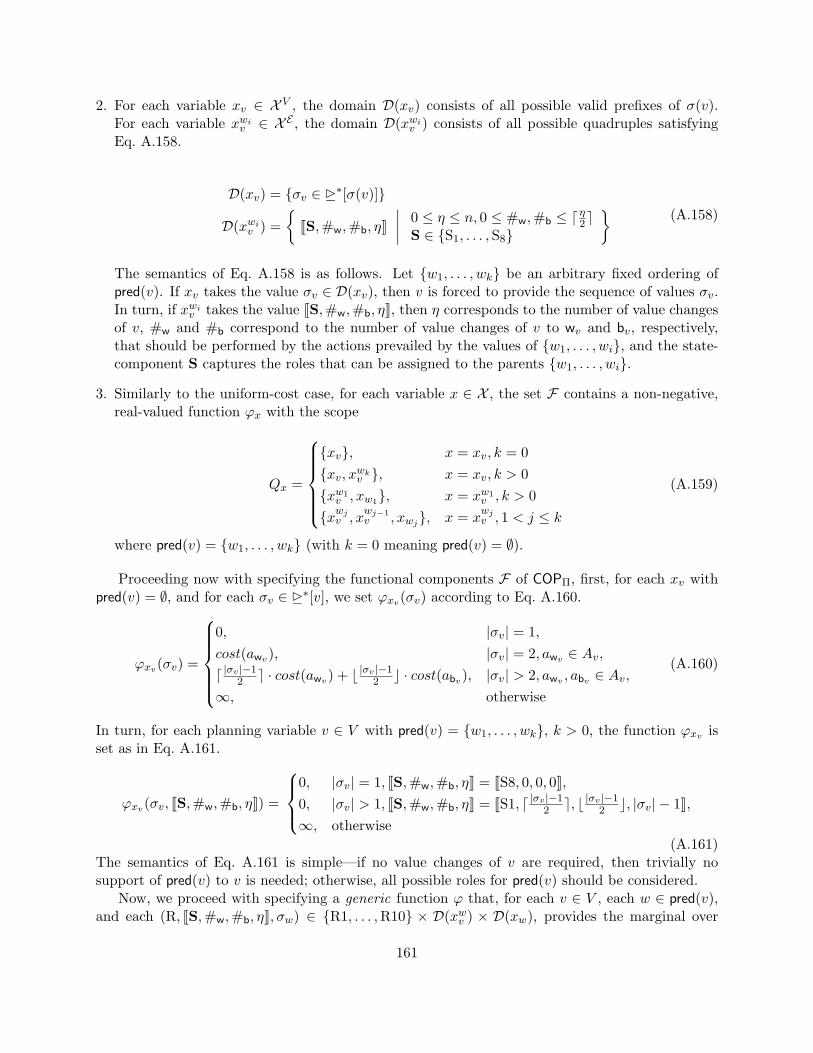
2. For each variable xv ∈ X V , the domain D(xv) consists of all possible valid prefixes of σ(v).For each variable xwiv ∈ X E , the domain D(xwiv ) consists of all possible quadruples satisfyingEq. A.158.
D(xv) = {σv ∈ �∗[σ(v)]}
D(xwiv ) ={
JS,#w,#b, ηK∣∣∣∣ 0 ≤ η ≤ n, 0 ≤ #w,#b ≤ dη2e
S ∈ {S1, . . . ,S8}
} (A.158)
The semantics of Eq. A.158 is as follows. Let {w1, . . . , wk} be an arbitrary fixed ordering ofpred(v). If xv takes the value σv ∈ D(xv), then v is forced to provide the sequence of values σv.In turn, if xwiv takes the value JS,#w,#b, ηK, then η corresponds to the number of value changesof v, #w and #b correspond to the number of value changes of v to wv and bv, respectively,that should be performed by the actions prevailed by the values of {w1, . . . , wi}, and the state-component S captures the roles that can be assigned to the parents {w1, . . . , wi}.
3. Similarly to the uniform-cost case, for each variable x ∈ X , the set F contains a non-negative,real-valued function ϕx with the scope
Qx =
{xv}, x = xv, k = 0{xv, xwkv }, x = xv, k > 0{xw1
v , xw1}, x = xw1v , k > 0
{xwjv , xwj−1v , xwj}, x = x
wjv , 1 < j ≤ k
(A.159)
where pred(v) = {w1, . . . , wk} (with k = 0 meaning pred(v) = ∅).
Proceeding now with specifying the functional components F of COPΠ, first, for each xv withpred(v) = ∅, and for each σv ∈ �∗[v], we set ϕxv(σv) according to Eq. A.160.
ϕxv(σv) =
0, |σv| = 1,cost(awv), |σv| = 2, awv ∈ Av,d |σv |−1
2 e · cost(awv) + b |σv |−12 c · cost(abv), |σv| > 2, awv , abv ∈ Av,
∞, otherwise
(A.160)
In turn, for each planning variable v ∈ V with pred(v) = {w1, . . . , wk}, k > 0, the function ϕxv isset as in Eq. A.161.
ϕxv(σv, JS,#w,#b, ηK) =
0, |σv| = 1, JS,#w,#b, ηK = JS8, 0, 0, 0K,0, |σv| > 1, JS,#w,#b, ηK = JS1, d |σv |−1
2 e, b |σv |−12 c, |σv| − 1K,
∞, otherwise(A.161)
The semantics of Eq. A.161 is simple—if no value changes of v are required, then trivially nosupport of pred(v) to v is needed; otherwise, all possible roles for pred(v) should be considered.
Now, we proceed with specifying a generic function ϕ that, for each v ∈ V , each w ∈ pred(v),and each (R, JS,#w,#b, ηK, σw) ∈ {R1, . . . ,R10} × D(xwv ) × D(xw), provides the marginal over
161
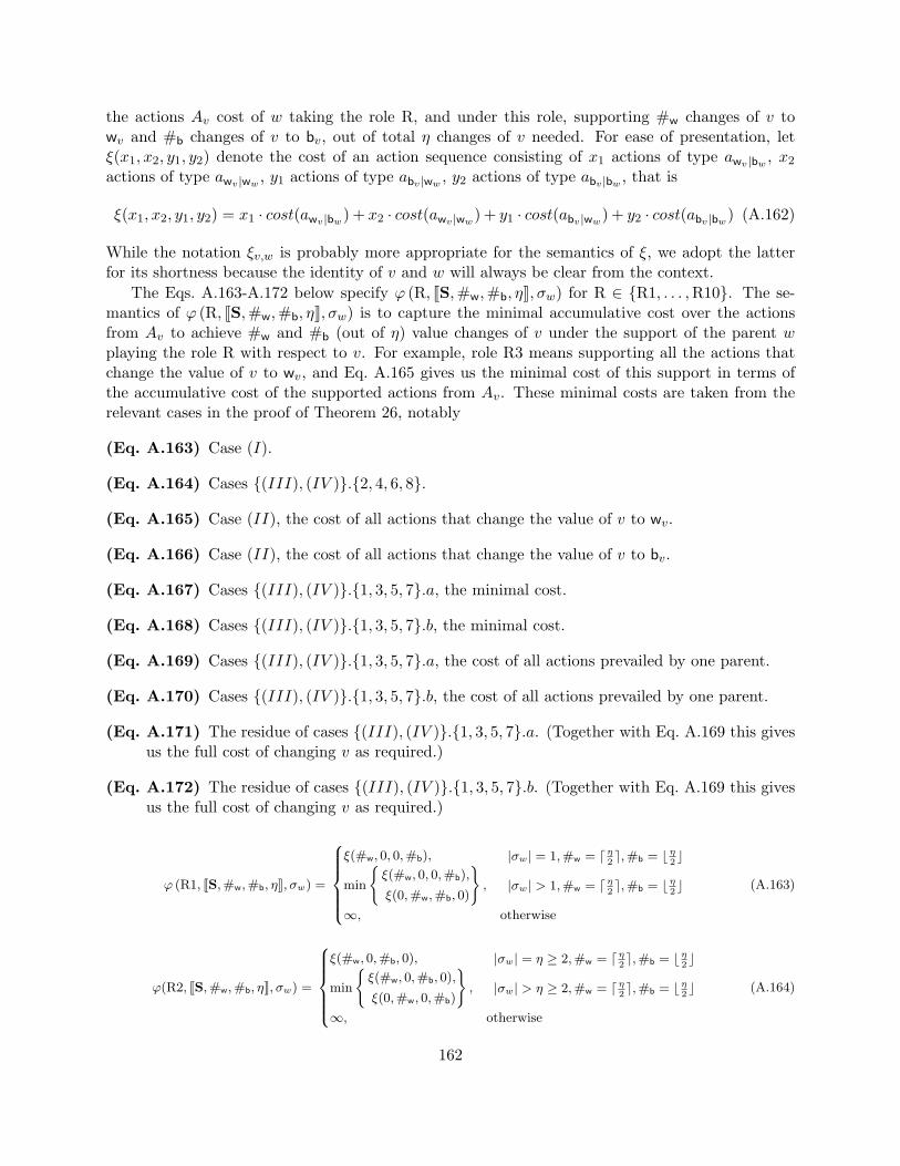
the actions Av cost of w taking the role R, and under this role, supporting #w changes of v towv and #b changes of v to bv, out of total η changes of v needed. For ease of presentation, letξ(x1, x2, y1, y2) denote the cost of an action sequence consisting of x1 actions of type awv |bw , x2
actions of type awv |ww , y1 actions of type abv |ww , y2 actions of type abv |bw , that is
ξ(x1, x2, y1, y2) = x1 · cost(awv |bw) + x2 · cost(awv |ww) + y1 · cost(abv |ww) + y2 · cost(abv |bw) (A.162)
While the notation ξv,w is probably more appropriate for the semantics of ξ, we adopt the latterfor its shortness because the identity of v and w will always be clear from the context.
The Eqs. A.163-A.172 below specify ϕ (R, JS,#w,#b, ηK, σw) for R ∈ {R1, . . . ,R10}. The se-mantics of ϕ (R, JS,#w,#b, ηK, σw) is to capture the minimal accumulative cost over the actionsfrom Av to achieve #w and #b (out of η) value changes of v under the support of the parent wplaying the role R with respect to v. For example, role R3 means supporting all the actions thatchange the value of v to wv, and Eq. A.165 gives us the minimal cost of this support in terms ofthe accumulative cost of the supported actions from Av. These minimal costs are taken from therelevant cases in the proof of Theorem 26, notably
(Eq. A.163) Case (I).
(Eq. A.164) Cases {(III), (IV )}.{2, 4, 6, 8}.
(Eq. A.165) Case (II), the cost of all actions that change the value of v to wv.
(Eq. A.166) Case (II), the cost of all actions that change the value of v to bv.
(Eq. A.167) Cases {(III), (IV )}.{1, 3, 5, 7}.a, the minimal cost.
(Eq. A.168) Cases {(III), (IV )}.{1, 3, 5, 7}.b, the minimal cost.
(Eq. A.169) Cases {(III), (IV )}.{1, 3, 5, 7}.a, the cost of all actions prevailed by one parent.
(Eq. A.170) Cases {(III), (IV )}.{1, 3, 5, 7}.b, the cost of all actions prevailed by one parent.
(Eq. A.171) The residue of cases {(III), (IV )}.{1, 3, 5, 7}.a. (Together with Eq. A.169 this givesus the full cost of changing v as required.)
(Eq. A.172) The residue of cases {(III), (IV )}.{1, 3, 5, 7}.b. (Together with Eq. A.169 this givesus the full cost of changing v as required.)
ϕ (R1, JS,#w,#b, ηK, σw) =
8>>>><>>>>:ξ(#w, 0, 0,#b), |σw| = 1,#w = d η
2e,#b = b η
2c
min
(ξ(#w, 0, 0,#b),
ξ(0,#w,#b, 0)
), |σw| > 1,#w = d η
2e,#b = b η
2c
∞, otherwise
(A.163)
ϕ(R2, JS,#w,#b, ηK, σw) =
8>>>><>>>>:ξ(#w, 0,#b, 0), |σw| = η ≥ 2,#w = d η
2e,#b = b η
2c
min
(ξ(#w, 0,#b, 0),
ξ(0,#w, 0,#b)
), |σw| > η ≥ 2,#w = d η
2e,#b = b η
2c
∞, otherwise
(A.164)
162
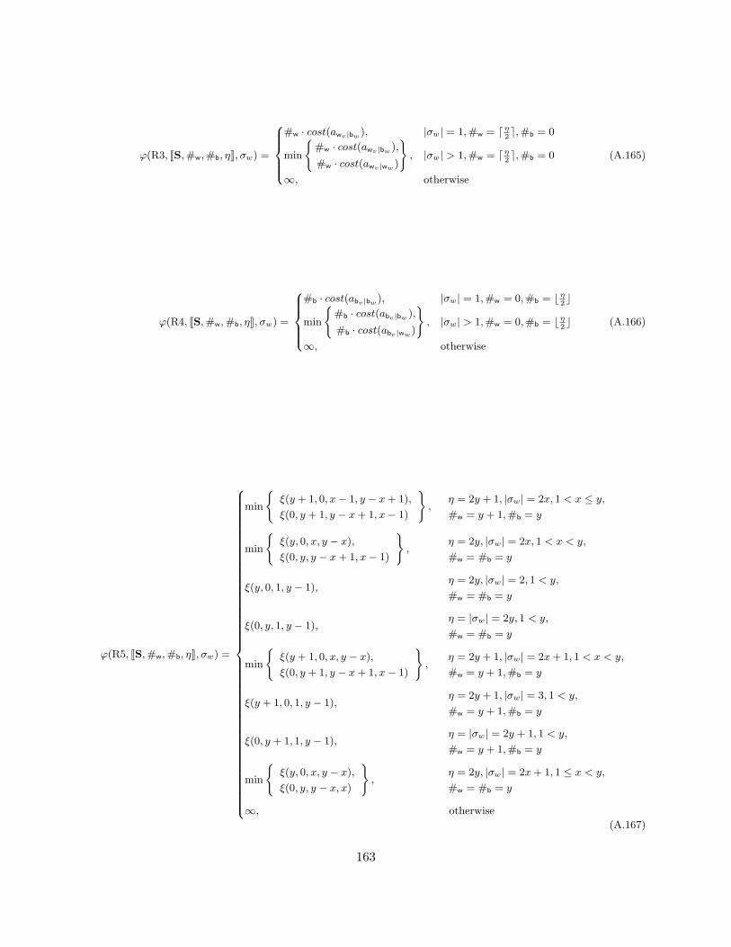
ϕ(R3, JS,#w,#b, ηK, σw) =
8>>><>>>:#w · cost(awv|bw ), |σw| = 1,#w = d η
2e,#b = 0
min
(#w · cost(awv|bw ),
#w · cost(awv|ww )
), |σw| > 1,#w = d η
2e,#b = 0
∞, otherwise
(A.165)
ϕ(R4, JS,#w,#b, ηK, σw) =
8>>><>>>:#b · cost(abv|bw ), |σw| = 1,#w = 0,#b = b η
2c
min
(#b · cost(abv|bw ),
#b · cost(abv|ww )
), |σw| > 1,#w = 0,#b = b η
2c
∞, otherwise
(A.166)
ϕ(R5, JS,#w,#b, ηK, σw) =
8>>>>>>>>>>>>>>>>>>>>>>>>>>>>>>>>>>>>>>>>>>>>><>>>>>>>>>>>>>>>>>>>>>>>>>>>>>>>>>>>>>>>>>>>>>:
min
(ξ(y + 1, 0, x− 1, y − x+ 1),
ξ(0, y + 1, y − x+ 1, x− 1)
),
η = 2y + 1, |σw| = 2x, 1 < x ≤ y,#w = y + 1,#b = y
min
(ξ(y, 0, x, y − x),
ξ(0, y, y − x+ 1, x− 1)
),
η = 2y, |σw| = 2x, 1 < x < y,
#w = #b = y
ξ(y, 0, 1, y − 1),η = 2y, |σw| = 2, 1 < y,
#w = #b = y
ξ(0, y, 1, y − 1),η = |σw| = 2y, 1 < y,
#w = #b = y
min
(ξ(y + 1, 0, x, y − x),
ξ(0, y + 1, y − x+ 1, x− 1)
),
η = 2y + 1, |σw| = 2x+ 1, 1 < x < y,
#w = y + 1,#b = y
ξ(y + 1, 0, 1, y − 1),η = 2y + 1, |σw| = 3, 1 < y,
#w = y + 1,#b = y
ξ(0, y + 1, 1, y − 1),η = |σw| = 2y + 1, 1 < y,
#w = y + 1,#b = y
min
(ξ(y, 0, x, y − x),
ξ(0, y, y − x, x)
),
η = 2y, |σw| = 2x+ 1, 1 ≤ x < y,
#w = #b = y
∞, otherwise
(A.167)
163
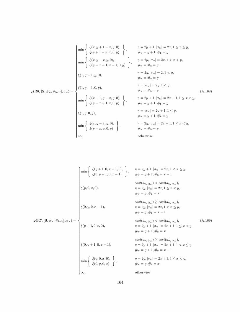
ϕ(R6, JS,#w,#b, ηK, σw) =
8>>>>>>>>>>>>>>>>>>>>>>>>>>>>>>>>>>>>>><>>>>>>>>>>>>>>>>>>>>>>>>>>>>>>>>>>>>>>:
min
(ξ(x, y + 1− x, y, 0),
ξ(y + 1− x, x, 0, y)
),
η = 2y + 1, |σw| = 2x, 1 ≤ x ≤ y,#w = y + 1,#b = y
min
(ξ(x, y − x, y, 0),
ξ(y − x+ 1, x− 1, 0, y)
),
η = 2y, |σw| = 2x, 1 < x < y,
#w = #b = y
ξ(1, y − 1, y, 0),η = 2y, |σw| = 2, 1 < y,
#w = #b = y
ξ(1, y − 1, 0, y),η = |σw| = 2y, 1 < y,
#w = #b = y
min
(ξ(x+ 1, y − x, y, 0),
ξ(y − x+ 1, x, 0, y)
),
η = 2y + 1, |σw| = 2x+ 1, 1 ≤ x < y,
#w = y + 1,#b = y
ξ(1, y, 0, y),η = |σw| = 2y + 1, 1 ≤ y,#w = y + 1,#b = y
min
(ξ(x, y − x, y, 0),
ξ(y − x, x, 0, y)
),
η = 2y, |σw| = 2x+ 1, 1 ≤ x < y,
#w = #b = y
∞, otherwise
(A.168)
ϕ(R7, JS,#w,#b, ηK, σw) =
8>>>>>>>>>>>>>>>>>>>>>>>>>>>>>>>>>>>>>>>>>>>>><>>>>>>>>>>>>>>>>>>>>>>>>>>>>>>>>>>>>>>>>>>>>>:
min
(ξ(y + 1, 0, x− 1, 0),
ξ(0, y + 1, 0, x− 1)
),
η = 2y + 1, |σw| = 2x, 1 < x ≤ y,#w = y + 1,#b = x− 1
ξ(y, 0, x, 0),
cost(awv|bw ) < cost(awv|ww ),
η = 2y, |σw| = 2x, 1 ≤ x < y,
#w = y,#b = x
ξ(0, y, 0, x− 1),
cost(awv|bw ) ≥ cost(awv|ww ),
η = 2y, |σw| = 2x, 1 < x ≤ y,#w = y,#b = x− 1
ξ(y + 1, 0, x, 0),
cost(awv|bw ) < cost(awv|ww ),
η = 2y + 1, |σw| = 2x+ 1, 1 ≤ x < y,
#w = y + 1,#b = x
ξ(0, y + 1, 0, x− 1),
cost(awv|bw ) ≥ cost(awv|ww ),
η = 2y + 1, |σw| = 2x+ 1, 1 < x ≤ y,#w = y + 1,#b = x− 1
min
(ξ(y, 0, x, 0),
ξ(0, y, 0, x)
),
η = 2y, |σw| = 2x+ 1, 1 ≤ x < y,
#w = y,#b = x
∞, otherwise
(A.169)
164
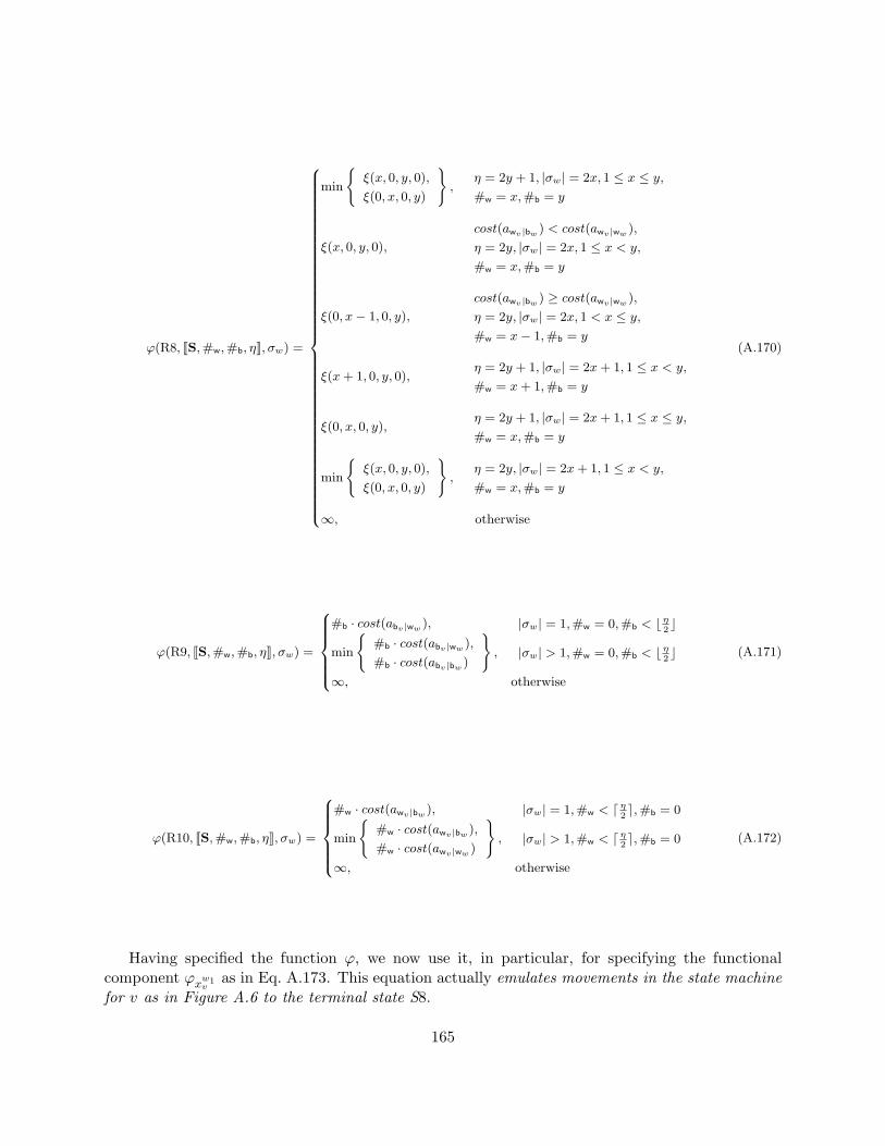
ϕ(R8, JS,#w,#b, ηK, σw) =
8>>>>>>>>>>>>>>>>>>>>>>>>>>>>>>>>>>>>>>>><>>>>>>>>>>>>>>>>>>>>>>>>>>>>>>>>>>>>>>>>:
min
(ξ(x, 0, y, 0),
ξ(0, x, 0, y)
),
η = 2y + 1, |σw| = 2x, 1 ≤ x ≤ y,#w = x,#b = y
ξ(x, 0, y, 0),
cost(awv|bw ) < cost(awv|ww ),
η = 2y, |σw| = 2x, 1 ≤ x < y,
#w = x,#b = y
ξ(0, x− 1, 0, y),
cost(awv|bw ) ≥ cost(awv|ww ),
η = 2y, |σw| = 2x, 1 < x ≤ y,#w = x− 1,#b = y
ξ(x+ 1, 0, y, 0),η = 2y + 1, |σw| = 2x+ 1, 1 ≤ x < y,
#w = x+ 1,#b = y
ξ(0, x, 0, y),η = 2y + 1, |σw| = 2x+ 1, 1 ≤ x ≤ y,#w = x,#b = y
min
(ξ(x, 0, y, 0),
ξ(0, x, 0, y)
),
η = 2y, |σw| = 2x+ 1, 1 ≤ x < y,
#w = x,#b = y
∞, otherwise
(A.170)
ϕ(R9, JS,#w,#b, ηK, σw) =
8>>>><>>>>:#b · cost(abv|ww ), |σw| = 1,#w = 0,#b < b η2 c
min
(#b · cost(abv|ww ),
#b · cost(abv|bw )
), |σw| > 1,#w = 0,#b < b η2 c
∞, otherwise
(A.171)
ϕ(R10, JS,#w,#b, ηK, σw) =
8>>>><>>>>:#w · cost(awv|bw ), |σw| = 1,#w < d η2 e,#b = 0
min
(#w · cost(awv|bw ),
#w · cost(awv|ww )
), |σw| > 1,#w < d η2 e,#b = 0
∞, otherwise
(A.172)
Having specified the function ϕ, we now use it, in particular, for specifying the functionalcomponent ϕxw1
vas in Eq. A.173. This equation actually emulates movements in the state machine
for v as in Figure A.6 to the terminal state S8.
165
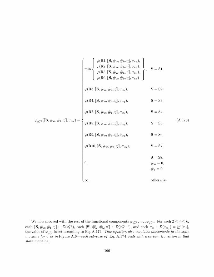
ϕxw1v
(JS,#w,#b, ηK, σw1) =
min
ϕ(R1, JS,#w,#b, ηK, σw1),ϕ(R2, JS,#w,#b, ηK, σw1),ϕ(R5, JS,#w,#b, ηK, σw1),ϕ(R6, JS,#w,#b, ηK, σw1)
, S = S1,
ϕ(R3, JS,#w,#b, ηK, σw1), S = S2,
ϕ(R4, JS,#w,#b, ηK, σw1), S = S3,
ϕ(R7, JS,#w,#b, ηK, σw1), S = S4,
ϕ(R8, JS,#w,#b, ηK, σw1), S = S5,
ϕ(R9, JS,#w,#b, ηK, σw1), S = S6,
ϕ(R10, JS,#w,#b, ηK, σw1), S = S7,
0,S = S8,#w = 0,#b = 0
∞, otherwise
(A.173)
We now proceed with the rest of the functional components ϕxw2v, . . . , ϕxwkv . For each 2 ≤ j ≤ k,
each JS,#w,#b, ηK ∈ D(xwjv ), each JS′,#′w,#′b, η′K ∈ D(xwj−1
v ), and each σw ∈ D(xwj ) = �∗[wj ],the value of ϕ
xwjv
is set according to Eq. A.174. This equation also emulates movements in the statemachine for v as in Figure A.6—each sub-case of Eq. A.174 deals with a certain transition in thatstate machine.
166
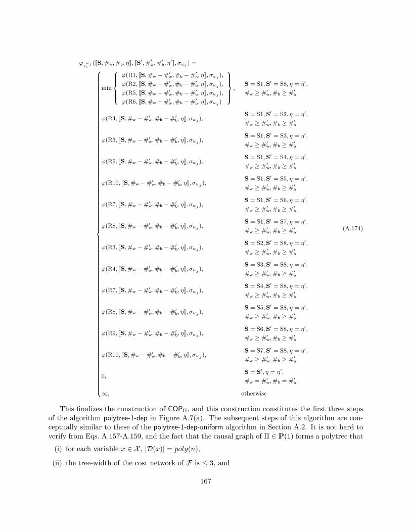
ϕx
wjv
(JS,#w,#b, ηK, JS′,#′w,#′b, η′K, σwj ) =8>>>>>>>>>>>>>>>>>>>>>>>>>>>>>>>>>>>>>>>>>>>>>>>>>>>>>>>>>>>>>>>>>>>>>>>>>>>>>>>>>>>><>>>>>>>>>>>>>>>>>>>>>>>>>>>>>>>>>>>>>>>>>>>>>>>>>>>>>>>>>>>>>>>>>>>>>>>>>>>>>>>>>>>>:
min
8>>><>>>:ϕ(R1, JS,#w −#′w,#b −#′b, ηK, σwj ),
ϕ(R2, JS,#w −#′w,#b −#′b, ηK, σwj ),
ϕ(R5, JS,#w −#′w,#b −#′b, ηK, σwj ),
ϕ(R6, JS,#w −#′w,#b −#′b, ηK, σwj )
9>>>=>>>; ,S = S1,S′ = S8, η = η′,
#w ≥ #′w,#b ≥ #′b
ϕ(R4, JS,#w −#′w,#b −#′b, ηK, σwj ),S = S1,S′ = S2, η = η′,
#w ≥ #′w,#b ≥ #′b
ϕ(R3, JS,#w −#′w,#b −#′b, ηK, σwj ),S = S1,S′ = S3, η = η′,
#w ≥ #′w,#b ≥ #′b
ϕ(R9, JS,#w −#′w,#b −#′b, ηK, σwj ),S = S1,S′ = S4, η = η′,
#w ≥ #′w,#b ≥ #′b
ϕ(R10, JS,#w −#′w,#b −#′b, ηK, σwj ),S = S1,S′ = S5, η = η′,
#w ≥ #′w,#b ≥ #′b
ϕ(R7, JS,#w −#′w,#b −#′b, ηK, σwj ),S = S1,S′ = S6, η = η′,
#w ≥ #′w,#b ≥ #′b
ϕ(R8, JS,#w −#′w,#b −#′b, ηK, σwj ),S = S1,S′ = S7, η = η′,
#w ≥ #′w,#b ≥ #′b
ϕ(R3, JS,#w −#′w,#b −#′b, ηK, σwj ),S = S2,S′ = S8, η = η′,
#w ≥ #′w,#b ≥ #′b
ϕ(R4, JS,#w −#′w,#b −#′b, ηK, σwj ),S = S3,S′ = S8, η = η′,
#w ≥ #′w,#b ≥ #′b
ϕ(R7, JS,#w −#′w,#b −#′b, ηK, σwj ),S = S4,S′ = S8, η = η′,
#w ≥ #′w,#b ≥ #′b
ϕ(R8, JS,#w −#′w,#b −#′b, ηK, σwj ),S = S5,S′ = S8, η = η′,
#w ≥ #′w,#b ≥ #′b
ϕ(R9, JS,#w −#′w,#b −#′b, ηK, σwj ),S = S6,S′ = S8, η = η′,
#w ≥ #′w,#b ≥ #′b
ϕ(R10, JS,#w −#′w,#b −#′b, ηK, σwj ),S = S7,S′ = S8, η = η′,
#w ≥ #′w,#b ≥ #′b
0,S = S′, η = η′,
#w = #′w,#b = #′b
∞, otherwise
(A.174)
This finalizes the construction of COPΠ, and this construction constitutes the first three stepsof the algorithm polytree-1-dep in Figure A.7(a). The subsequent steps of this algorithm are con-ceptually similar to these of the polytree-1-dep-uniform algorithm in Section A.2. It is not hard toverify from Eqs. A.157-A.159, and the fact that the causal graph of Π ∈ P(1) forms a polytree that
(i) for each variable x ∈ X , |D(x)| = poly(n),
(ii) the tree-width of the cost network of F is ≤ 3, and
167
(iii) the optimal tree-decomposition of the COPΠ’s cost network is given by any topological orderingof the causal graph that is consistent with the (arbitrary yet fixed at the time of the COPΠ’sconstruction) orderings of each planning variable’s parents in the causal graph.
procedure polytree-1-dep(Π = 〈V ,A, I ,G, cost〉)takes a planning task Π ∈ P(1)returns a cost-optimal plan for Π if Π is solvable, and fails otherwise
create a set of variables X as in Eqs. A.157-A.158create a set of functions F = {ϕx | x ∈ X} with scopes as in Eq. A.159for each x ∈ X do
specify ϕx according to Eqs. A.160-A.174endforset COPΠ := (X ,F) with global objective min
∑ϕ∈F ϕ(X )
x := solve-tree-cop(COPΠ)if∑
ϕ∈F ϕ(x) =∞ then return failureextract plan ρ from x with cost(ρ) =
∑ϕ∈F ϕ(x)
return ρ
Figure A.7: Algorithm for cost-optimal planning for P(1) tasks.
A.3.3 Correctness and Complexity
Lemma 11 Let Π be a P(1) task, COPΠ = (X ,F) be the corresponding constraint optimizationproblem, and x be an optimal assignment to X with
∑ϕ∈F ϕ(x) = α.
(I) If α <∞, then a plan of cost α for Π can be reconstructed from x in time polynomial in thedescription size of Π.
(II) If Π has a plan, then α <∞.
Proof:(I) Given a COP solution x with
∑ϕ∈F ϕ(x) = α <∞, we construct a plan ρ for Π with cost(ρ) = α.
We construct this plan by
1. Traversing the planning variables in a topological ordering of the causal graph CG(Π), andassociating each variable v with a sequence ρv ∈ A∗v.
2. Merging the constructed sequences ρv1 , . . . , ρvn into the desired plan ρ.
For each v ∈ V with pred(v) = ∅ we set ρv = 〈a1 · . . . · al〉, where l = |xv| − 1, and ai is defined asin Eq A.175 below.
ai =
{awv , i is odd,abv , i is even,
(A.175)
Note that Eq. A.175 is well-defined—the existence of the essential for Eq. A.175 actions awv/abv isimplied by Eq. A.160 and α <∞.
In turn, for each v ∈ V with pred(v) = {w1, . . . , wk}, given xw1v , . . . , xwkv , we distinguish between
the following cases.
168
[ R1 is played ] R1 is played by one of the parents, while all other parents play role R11.
[ R1 is played by w1 ] Eq. A.173 then implies
ϕxw1v
(xw1v , xw1) = ϕ(R1, xw1
v , xw1)
and xw1v 3 S = S1. From Eq. A.174 we then have xwjv 3 S′ = S1 for each 1 < j ≤ k,
giving usϕxwjv
(xwjv , xwj−1v , xwj ) = 0.
[ R1 is played by wj, j > 1 ] Eq. A.174 then implies
ϕxwjv
(JS,#w,#b, ηK, JS′,#′w,#′b, η′K, σwj ) = ϕ(R1, JS,#w −#′w,#b −#′b, ηK, σwj )
and, for all 1 < i 6= j ≤ k,ϕxwiv (xwiv , x
wi−1v , xwi) = 0.
From Eq. A.173 we also haveϕxw1
v(xw1v , xw1) = 0.
In both these sub-cases, ρv, >v and >v,w are specified as in the proof of Theorem 26, case I.
[ R2 is played ] R2 is played by one of the parents, while all other parents play role R11.
[ R2 is played by w1 ] Eq. A.173 then implies
ϕxw1v
(xw1v , xw1) = ϕ(R2, xw1
v , xw1)
and, for each 1 < j ≤ k, Eq. A.174 implies
ϕxwjv
(xwjv , xwj−1v , xwj ) = 0.
If ϕ(R2, JS,#w,#b, ηK, σw1) = ξ(#w, 0,#b, 0), then ρv, >v and >v,w are specified as inthe proof of Theorem 26, case III.2, otherwise, as in the case IV.2.
[ R2 is played by wj, j > 1 ] Eq. A.174 then implies
ϕxwjv
(JS,#w,#b, ηK, JS′,#′w,#′b, η′K, σwj ) = ϕ(R2, JS,#w −#′w,#b −#′b, ηK, σwj )
and, for all 1 < i 6= j ≤ k,ϕxwiv (xwiv , x
wi−1v , xwi) = 0.
From Eq. A.173 we also haveϕxw1
v(xw1v , xw1) = 0.
If ϕ(R2, JS,#w −#′w,#b −#′b, ηK, σwj ) = ξ(#w −#′w, 0,#b −#′b, 0), then ρv, >v and>v,w are specified as in the proof of Theorem 26, case III.2, otherwise, as in the caseIV.2.
[ R3 and R4 are played ] Those roles are played by two of the parents, while all other parentsplay role R11.
169
[ R3 is played by w1, R4 is played by wj, j > 1 ] From Eqs. A.173 and A.174 we thenhave
ϕxw1v
(xw1v , xw1) = ϕ(R3, xw1
v , xw1),
ϕxwjv
(JS,#w,#b, ηK, JS′,#′w,#′b, η′K, σwj ) = ϕ(R4, JS,#w −#′w,#b −#′b, ηK, σwj ),
and, for all 1 < i ≤ k, such that i 6= j:
ϕxwiv (xwiv , xwi−1v , xwi) = 0.
[ R4 is played by w1, R3 is played by wj, j > 1 ] From Eqs. A.173 and A.174 we thenhave
ϕxw1v
(xw1v , xw1) = ϕ(R4, xw1
v , xw1),
ϕxwjv
(JS,#w,#b, ηK, JS′,#′w,#′b, η′K, σwj ) = ϕ(R3, JS,#w −#′w,#b −#′b, ηK, σwj ),
and, for all 1 < i 6= j ≤ k,ϕxwiv (xwiv , x
wi−1v , xwi) = 0.
[ R3 is played by wj, R4 is played by wt, j 6= t, j, t > 1 ] From Eqs. A.173 and A.174we have
ϕxw1v
(xw1v , xw1) = 0,
ϕxwjv
(JS,#w,#b, ηK, JS′,#′w,#′b, η′K, σwj ) = ϕ(R3, JS,#w −#′w,#b −#′b, ηK, σwj ),
ϕxwtv (JS,#w,#b, ηK, JS′,#′w,#′b, η′K, σwt) = ϕ(R4, JS,#w −#′w,#b −#′b, ηK, σwt),
and, for all 1 < i ≤ k such that i 6∈ {j, t},
ϕxwiv (xwiv , xwi−1v , xwi) = 0
In all these three sub-cases, ρv, >v and >v,w are specified as in the proof of Theorem 26, caseII.
[ R5 is played ] R5 is played by one of the parents, while all other parents play role R11.
[ R5 is played by w1 ] Eqs. A.173 and A.174 imply
ϕxw1v
(xw1v , xw1) = ϕ(R5, xw1
v , xw1),
and, for each 1 < j ≤ k,ϕxwjv
(xwjv , xwj−1v , xwj ) = 0.
Considering now the specification of the function ϕ in Eq. A.167,
• If the first case holds, and the minimum is obtained at the first expression, then ρv,>v and >v,w are defined as in the proof of Theorem 26, case III.1.a.• If the first case holds, and the minimum is obtained at the second expression, thenρv, >v and >v,w are defined as in the proof of Theorem 26, case IV.1.a.• If the second case holds, and the minimum is obtained at the first expression, thenρv, >v and >v,w are defined as in the proof of Theorem 26, case III.3.a.
170
• If the second case holds, and the minimum is obtained at the second expression,then ρv, >v and >v,w are defined as in the proof of Theorem 26, case IV.3.a.• If the third case holds, then ρv, >v and >v,w are defined as in the proof of Theo-
rem 26, case III.3.a.• If the forth case holds, then ρv, >v and >v,w are defined as in the proof of Theo-
rem 26, case IV.3.a.• If the fifth case holds, and the minimum is obtained at the first expression, then ρv,>v and >v,w are defined as in the proof of Theorem 26, case III.5.a.• If the fifth case holds, and the minimum is obtained at the second expression, thenρv, >v and >v,w are defined as in the proof of Theorem 26, case IV.5.a.• If the sixth case holds, then ρv, >v and >v,w are defined as in the proof of Theo-
rem 26, case III.5.a.• If the seventh case holds, then ρv, >v and >v,w are defined as in the proof of
Theorem 26, case IV.5.a.• If the eighth case holds, and the minimum is obtained at the first expression, thenρv, >v and >v,w are defined as in the proof of Theorem 26, case III.7.a.• If the eighth case holds, and the minimum is obtained at the second expression, thenρv, >v and >v,w are defined as in the proof of Theorem 26, case IV.7.a.
[ R5 is played by wj, j > 1 ] Eq. A.174 then implies
ϕxwjv
(JS,#w,#b, ηK, JS′,#′w,#′b, η′K, σwj ) = ϕ(R5, JS,#w −#′w,#b −#′b, ηK, σwj ),
and, for all 1 < i 6= j ≤ k,ϕxwiv (xwiv , x
wi−1v , xwi) = 0.
From Eq. A.173 we also haveϕxw1
v(xw1v , xw1) = 0.
Here ρv, >v and >v,w are specified exactly as in the previous case.
[ R6 is played ] R6 is played by one of the parents, while all other parents play role R11.
[ R6 is played by w1 ] Eqs. A.173 and A.174 imply
ϕxw1v
(xw1v , xw1) = ϕ(R6, xw1
v , xw1),
and, for each 1 < j ≤ k,ϕxwjv
(xwjv , xwj−1v , xwj ) = 0.
Considering now the specification of the function ϕ in Eq. A.168,
• If the first case holds, and the minimum is obtained at the first expression, then ρv,>v and >v,w are defined as in the proof of Theorem 26, case III.1.b.• If the first case holds, and the minimum is obtained at the second expression, thenρv, >v and >v,w are defined as in the proof of Theorem 26, case IV.1.b.• If the second case holds, and the minimum is obtained at the first expression, thenρv, >v and >v,w are defined as in the proof of Theorem 26, case III.3.b.
171
• If the second case holds, and the minimum is obtained at the second expression,then ρv, >v and >v,w are defined as in the proof of Theorem 26, case IV.3.b.• If the third case holds, then ρv, >v and >v,w are defined as in the proof of Theo-
rem 26, case III.3.b.• If the forth case holds, then ρv, >v and >v,w are defined as in the proof of Theo-
rem 26, case IV.3.b.• If the fifth case holds, and the minimum is obtained at the first expression, then ρv,>v and >v,w are defined as in the proof of Theorem 26, case III.5.b.• If the fifth case holds, and the minimum is obtained at the second expression, thenρv, >v and >v,w are defined as in the proof of Theorem 26, case IV.5.b.• If the sixth case holds, then ρv, >v and >v,w are defined as in the proof of Theo-
rem 26, case III.5.b.• If the seventh case holds, and the minimum is obtained at the first expression, thenρv, >v and >v,w are defined as in the proof of Theorem 26, case III.7.b.• If the seventh case holds, and the minimum is obtained at the second expression,
then ρv, >v and >v,w are defined as in the proof of Theorem 26, case IV.7.b.
[ R6 is played by wj, j > 1 ] Eq. A.174 then implies
ϕxwjv
(JS,#w,#b, ηK, JS′,#′w,#′b, η′K, σwj ) = ϕ(R6, JS,#w −#′w,#b −#′b, ηK, σwj ),
and, for all 1 < i 6= j ≤ k,ϕxwiv (xwiv , x
wi−1v , xwi) = 0.
From Eq. A.173 we also haveϕxw1
v(xw1v , xw1) = 0.
Here ρv, >v and >v,w are specified exactly as in the previous case.
[ R7 and R9 are played ] Those roles are played by two of the parents, while all other parentsplay role R11.
[ R7 is played by w1, R9 is played by wj, j > 1 ] From Eqs. A.173 and A.174 we thenhave
ϕxw1v
(xw1v , xw1) = ϕ(R7, xw1
v , xw1),
ϕxwjv
(JS,#w,#b, ηK, JS′,#′w,#′b, η′K, σwj ) = ϕ(R9, JS,#w −#′w,#b −#′b, ηK, σwj ),
and ,for all 1 < i 6= j ≤ k,ϕxwiv (xwiv , x
wi−1v , xwi) = 0.
Considering now the specification of the function ϕ in Eq. A.169,
• If the first case holds, and the minimum is obtained at the first expression, then ρv,>v and >v,w are defined as in the proof of Theorem 26, case III.1.a.• If the first case holds, and the minimum is obtained at the second expression, thenρv, >v and >v,w are defined as in the proof of Theorem 26, case IV.1.a.• If the second case holds, then ρv, >v and >v,w are defined as in the proof of Theo-
rem 26, case III.3.a.
172
• If the third case holds, then ρv, >v and >v,w are defined as in the proof of Theo-rem 26, case IV.3.a.• If the forth case holds, then ρv, >v and >v,w are defined as in the proof of Theo-
rem 26, case III.5.a.• If the fifth case holds, then ρv, >v and >v,w are defined as in the proof of Theorem 26,
case IV.5.a.• If the sixth case holds, and the minimum is obtained at the first expression, thenρv, >v and >v,w are defined as in the proof of Theorem 26, case III.7.a.• If the sixth case holds, and the minimum is obtained at the second expression, thenρv, >v and >v,w are defined as in the proof of Theorem 26, case IV.7.a.
[ R9 is played by w1, R7 is played by wj, j > 1 ] From Eqs. A.173 and A.174 we thenhave
ϕxw1v
(xw1v , xw1) = ϕ(R9, xw1
v , xw1),
ϕxwjv
(JS,#w,#b, ηK, JS′,#′w,#′b, η′K, σwj ) = ϕ(R7, JS,#w −#′w,#b −#′b, ηK, σwj ),
and, for all 1 < i 6= j ≤ k,ϕxwiv (xwiv , x
wi−1v , xwi) = 0.
Here ρv, >v and >v,w are specified exactly as in the previous case.
[ R7 is played by wj, R9 is played by wt, j 6= t, j, t > 1 ] From Eqs. A.173 and A.174we have
ϕxw1v
(xw1v , xw1) = 0,
ϕxwjv
(JS,#w,#b, ηK, JS′,#′w,#′b, η′K, σwj ) = ϕ(R7, JS,#w −#′w,#b −#′b, ηK, σwj ),
ϕxwtv (JS,#w,#b, ηK, JS′,#′w,#′b, η′K, σwt) = ϕ(R9, JS,#w −#′w,#b −#′b, ηK, σwt),
and, for all 1 < i ≤ k, such that i 6∈ {j, t},
ϕxwiv (xwiv , xwi−1v , xwi) = 0.
Then, ρv, >v and >v,w are specified exactly as in the two previous cases.
[ R8 and R10 are played ] Those roles are played by two of the parents, while all other parentsplay role R11.
[ R8 is played by w1, R10 is played by wj, j > 1 ] From Eqs. A.173 and A.174 we thenhave
ϕxw1v
(xw1v , xw1) = ϕ(R8, xw1
v , xw1),
ϕxwjv
(JS,#w,#b, ηK, JS′,#′w,#′b, η′K, σwj ) = ϕ(R10, JS,#w −#′w,#b −#′b, ηK, σwj ),
and, for all 1 < i 6= j ≤ k,ϕxwiv (xwiv , x
wi−1v , xwi) = 0.
Considering now the specification of the function ϕ in Eq. A.170,
• If the first case holds, and the minimum is obtained at the first expression, then ρv,>v and >v,w are defined as in the proof of Theorem 26, case III.1.b.
173
• If the first case holds, and the minimum is obtained at the second expression, thenρv, >v and >v,w are defined as in the proof of Theorem 26, case IV.1.b.• If the second case holds, then ρv, >v and >v,w are defined as in the proof of Theo-
rem 26, case III.3.b.• If the third case holds, then ρv, >v and >v,w are defined as in the proof of Theo-
rem 26, case IV.3.b.• If the forth case holds, then ρv, >v and >v,w are defined as in the proof of Theo-
rem 26, case III.5.b.• If the fifth case holds, then ρv, >v and >v,w are defined as in the proof of Theorem 26,
case IV.5.b.• If the sixth case holds, and the minimum is obtained at the first expression, thenρv, >v and >v,w are defined as in the proof of Theorem 26, case III.7.b.• If the sixth case holds, and the minimum is obtained at the second expression, thenρv, >v and >v,w are defined as in the proof of Theorem 26, case IV.7.b.
[ R10 is played by w1, R8 is played by wj, j > 1 ] From Eqs. A.173 and A.174 we thenhave
ϕxw1v
(xw1v , xw1) = ϕ(R10, xw1
v , xw1),
ϕxwjv
(JS,#w,#b, ηK, JS′,#′w,#′b, η′K, σwj ) = ϕ(R8, JS,#w −#′w,#b −#′b, ηK, σwj ),
and, for all 1 < i 6= j ≤ k,ϕxwiv (xwiv , x
wi−1v , xwi) = 0.
Here ρv, >v and >v,w are specified exactly as in the previous case.
[ R8 is played by wj, R10 is played by wt, j 6= t, j, t > 1 ] From Eqs. A.173 and A.174we have
ϕxw1v
(xw1v , xw1) = 0,
ϕxwjv
(JS,#w,#b, ηK, JS′,#′w,#′b, η′K, σwj ) = ϕ(R8, JS,#w −#′w,#b −#′b, ηK, σwj ),
ϕxwtv (JS,#w,#b, ηK, JS′,#′w,#′b, η′K, σwt) = ϕ(R10, JS,#w −#′w,#b −#′b, ηK, σwt),
and, for all 1 < i ≤ k, such that i 6∈ {j, t},
ϕxwiv (xwiv , xwi−1v , xwi) = 0.
Then, ρv, >v and >v,w are specified exactly as in the two previous cases.
Until now, for each variable v ∈ V , we have specified the action sequence ρv and the order>v over the elements of ρv. For each w ∈ pred(v), we have specified the order >v,w, and provedthat all >v ∪ >v,w and >w ∪ >v,w form strict partial orders over their domains. Similarly to theuniform cost case, this construction allows us to apply now Theorem 22 on the (considered as sets)sequences ρv and orders >v and >v,w, proving that
>=⋃v∈V
(>v ∪⋃
w∈pred(v)
>v,w)
forms a strict partial order over the union of ρv1 , . . . , ρvn .
174
Finally, we note that the plan extraction step of the algorithm polytree-1-dep corresponds ex-actly to the above construction along Eqs. A.52-A.57, A.59-A.61, A.63-A.64, A.71-A.72, A.74-A.75, A.83-A.84, A.86, A.88, A.95-A.96, A.98, A.100, A.107-A.108, A.110-A.111, A.113, A.120-A.121, A.123, A.131-A.132, A.134-A.135, A.137, A.144-A.145, A.147-A.148, A.156, providing us inpoly-time with concrete cost-optimal plan corresponding to the optimal solution for COPΠ.
(II) We now prove that if Π is solvable, then we must have α < ∞. Assume to the contrary thatthis is not the case. Let Π be a solvable P(1) task, and let (using Theorem 26) ρ be an irreducible,post-3/2 plan for Π. Given such ρ, let a COP assignment xρ be defined as follows.
1. For each COP variable xv, the assignment xρ provides the value σv ∈ �∗[σ(v)] such that|σv| = |ρ↓v |+ 1.
2. For each variable v ∈ V , such that pred(v) 6= ∅, find the (at most two) parents that prevail theactions in ρ[v]. Let w be such a parent that performs a role R ∈ {R1,R2,R3,R5,R6,R7,R8},and w′ be the other such parent that performs one of the roles R′ ∈ {R4,R9,R10,R11}. (Bydefinition of post-3/2 action sequences, the rest of the parents all perform role R11.) Giventhat, if |pred(v)| = k > 0, we adopt an ordering of pred(v) such that w1 = w and wk = w′.First, the assignment xwkv to COP variable xwkv provides the value JS1, d |σv |−1
2 e, b |σv |−12 c, |σv|−
1K. Then, for 1 ≤ i < k, the assignment xwiv to COP variable xwiv provides the valueJS,#w,#b, |σv| − 1K, where
S =
S2, R′ = R4S4, R′ = R9S5, R′ = R10S1, R′ = R11
and #w and #b are the numbers of actions in ρ↓v that change the value of v to wv and bv,respectively, while being prevailed by the value of w1.
From Eq. A.160-A.174 we then have that, for each v ∈ V , if pred(v) = ∅, then ϕxv(xv) = cost(ρ↓v). Otherwise, if pred(v) = {w1, . . . , wk}, then ϕxv(xv, xwkv ) = 0, and
∑w∈pred(v) ϕxwv (xρ) = cost(ρ↓v).
Therefore, we have ∑ϕ∈F
ϕ(xρ) =∑v∈V
cost(ρ↓v) = cost(ρ),
which is what we had to prove.
Theorem 27 Cost-optimal planning for P(1) is tractable.
Proof: The correctness of the polytree-1-dep algorithm is given by Lemma 11. We now show that,given a planning task Π ∈ P(1), the corresponding constraint optimization problem COPΠ can beconstructed and solved in time polynomial in the description size of Π.
Let n be the number of state variables in Π. In polytree-1-dep-uniform, we first construct theconstraint optimization problem COPΠ over Θ(n2) variables X with domain sizes being boundedeither by O(n) or by O(n3) (for COP variables representing state variables and causal graph edges,respectively). The number of functional components in COPΠ is Θ(n2), each defined over onevariable with domain size of O(n) and either one or two variables with domain sizes of O(n3). Theconstruction is linear in the size of the resulting COP, and thus is accomplished in time O(n9).
175
Applying then to COPΠ a tree-decomposition that clusters the scopes of the functional com-ponents F , we arrive into an equivalent, tree-structured constraint optimization problem overΘ(n2) variables with domains of size O(n7). Such a tree-structured COP can be solved in timeO(xy2) where x is the number of variables and y is an upper bound on the size of a variable’sdomain (Dechter, 2003). Therefore, solving COPΠ can be done in time O(n16). As this dominatesboth the time complexity of constructing COPΠ, and the time complexity of extracting a plan fromthe optimal solution to COPΠ (see the proof of (I) in Lemma 11), the overall complexity of thealgorithm polytree-1-dep-uniform is O(n16), and therefore polynomial in the description size of Π.
176
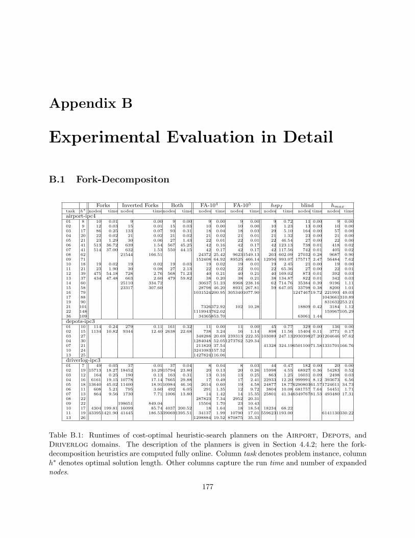
Appendix B
Experimental Evaluation in Detail
B.1 Fork-Decompositon
Forks Inverted Forks Both FA-104 FA-105 hspf blind hmaxtask h∗ nodes time nodes timenodes time nodes time nodes time nodes time nodes time nodes time
airport-ipc401 8 10 0.01 9 0.00 9 0.00 9 0.00 9 0.00 9 0.72 11 0.00 9 0.0002 9 12 0.03 15 0.01 15 0.03 10 0.00 10 0.00 10 1.23 13 0.00 10 0.0003 17 86 0.25 133 0.07 93 0.31 18 0.04 18 0.03 29 5.10 164 0.00 57 0.0004 20 22 0.02 21 0.02 21 0.02 21 0.02 21 0.01 21 1.32 23 0.00 21 0.0005 21 23 1.29 30 0.06 27 1.43 22 0.01 22 0.01 22 46.54 27 0.00 22 0.0006 41 513 36.72 639 1.54 567 45.25 42 0.16 42 0.17 42 123.13 738 0.01 418 0.0207 41 514 37.00 632 1.53 550 44.15 42 0.17 42 0.17 42 117.56 742 0.01 405 0.0208 62 21544 166.51 24372 25.42 96231549.13 203 602.09 27032 0.28 9687 0.9009 71 152408 64.92 89525 466.14 12956 993.07 175717 2.47 56484 7.6210 18 19 0.02 19 0.02 19 0.03 19 0.02 19 0.01 19 2.45 21 0.00 19 0.0011 21 23 1.90 30 0.08 27 2.13 22 0.02 22 0.01 22 65.36 27 0.00 22 0.0112 39 475 54.18 728 2.76 568 71.23 40 0.21 40 0.21 40 169.02 873 0.01 392 0.0313 37 434 47.48 663 2.60 479 59.82 38 0.20 38 0.21 38 134.87 822 0.01 342 0.0314 60 25110 334.72 30637 51.23 8968 238.16 62 714.76 35384 0.39 9196 1.1115 58 23317 307.60 28798 46.20 8931 267.81 59 647.05 33798 0.38 8200 1.0116 79 1031524200.95 3053401077.90 124746719.72 221993 49.0317 88 1043661310.8919 90 831632253.2121 101 7326372.92 102 10.28 18809 0.42 3184 1.1222 148 1119943762.02 159967105.2936 109 34365853.70 63061 1.44
depots-ipc301 10 114 0.24 279 0.11 161 0.32 11 0.00 11 0.00 45 0.77 329 0.00 136 0.0002 15 1134 10.82 9344 12.40 2638 22.68 738 3.24 16 1.14 898 11.56 15404 0.11 3771 0.1703 27 348288 20.69 239313 222.35 103089 247.13293039827.201204646 97.6204 30 1284048 52.051273762 529.3407 21 211820 37.54 41328 324.19650110071.581331701166.7610 24 3241083157.5213 25 1427824116.06
driverlog-ipc301 7 49 0.05 37 0.01 37 0.04 8 0.04 8 0.03 44 0.47 182 0.00 20 0.0002 19 15713 18.27 18452 10.2915794 23.80 20 0.13 20 0.26 15998 4.55 68927 0.36 54283 0.5203 12 164 0.25 190 0.13 163 0.31 13 0.16 13 0.25 863 1.25 16031 0.09 2498 0.0304 16 6161 19.15 10778 17.14 7665 29.88 17 0.49 17 2.41 22933 12.20 999991 8.12 393673 6.5605 18 13640 45.02 11400 18.9110984 46.16 2614 0.60 19 4.58 24877 18.77629080361.571724611 34.7306 11 608 5.21 795 3.60 492 6.05 291 1.35 12 9.72 3804 10.08 681757 7.64 54451 1.7107 13 864 9.56 1730 7.71 1006 13.80 14 1.42 14 15.35 25801 41.34634976781.53 493480 17.3108 22 287823 7.34 2952 20.3109 22 198651 849.04 15504 1.70 23 10.4310 17 4304 199.81 16099 85.74 4037 200.52 18 1.64 18 18.54 18234 68.2211 19 433951421.90 41445 186.53390691395.51 34137 1.99 10790 17.01 5596231193.00 6141130330.2213 26 1298884 19.52 870875 35.33
Table B.1: Runtimes of cost-optimal heuristic-search planners on the Airport, Depots, andDriverlog domains. The description of the planners is given in Section 4.4.2; here the fork-decomposition heuristics are computed fully online. Column task denotes problem instance, columnh∗ denotes optimal solution length. Other columns capture the run time and number of expandednodes.
177
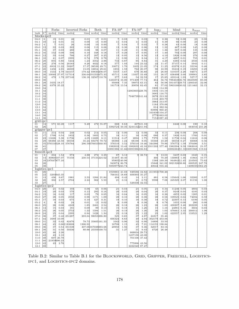
Forks Inverted Forks Both FA-104 FA-105 hspf blind hmaxtask h∗ nodes time nodes time nodes time nodes time nodes time nodes time nodes time nodes time
blocks-ipc204-0 6 15 0.01 46 0.01 17 0.01 7 0.03 7 0.03 7 0.36 93 0.00 25 0.0004-1 10 14 0.01 31 0.00 15 0.00 11 0.04 11 0.03 11 0.39 66 0.00 23 0.0004-2 6 7 0.01 26 0.00 10 0.00 7 0.04 7 0.03 7 0.38 63 0.00 18 0.0005-0 12 32 0.03 302 0.06 113 0.08 13 0.30 13 0.96 13 1.32 467 0.00 145 0.0005-1 10 37 0.03 280 0.06 98 0.07 11 0.29 11 0.96 11 1.36 567 0.00 135 0.0005-2 16 152 0.09 596 0.10 348 0.18 17 0.29 17 0.95 17 1.49 792 0.00 297 0.0006-0 12 33 0.04 766 0.27 207 0.25 13 0.95 13 8.56 13 4.10 1826 0.00 276 0.0006-1 10 41 0.07 2395 0.74 578 0.78 11 0.90 11 8.34 11 4.17 4887 0.01 755 0.0106-2 20 855 0.80 5444 1.23 3352 2.88 733 0.87 85 8.84 31 4.29 6385 0.02 2556 0.0307-0 20 278 0.56 20183 8.26 4022 8.18 577 1.93 144 23.32 22 11.47 37157 0.14 5943 0.1107-1 22 6910 11.22 59207 17.37 38539 49.71 10071 1.70 1835 21.05 174 11.25 63376 0.21 33194 0.4607-2 20 1458 2.85 46009 15.05 18854 29.61 1855 1.59 782 20.37 90 10.99 55218 0.19 18293 0.2908-0 18 1533 4.79 344157 179.42 69830208.07 5557 3.67 678 36.80 25 26.00 519107 2.28 94671 2.0708-1 20 10040 27.97 517514 236.64191352475.33 45711 3.88 11827 33.49 151 26.57 636498 2.60 199901 3.8508-2 16 479 1.79 237140 136.18 32567110.76 277 3.63 54 32.53 17 25.85 433144 1.93 52717 1.3009-0 30 1233374 16.00 971409 77.74 464 56.76 798464936.76 3840589 85.0009-1 28 3435 18.17 95068 7.35 58873 63.15 82 56.98 591457229.73 1200345 32.0609-2 26 6379 35.22 161719 13.54 20050 82.45 81 57.02 596316030.02 1211463 32.1510-0 34 1800 114.2610-1 32 12063665228.76 1835 115.1910-2 34 3685 116.7511-0 32 7046739141.44 2678 213.3211-1 30 1510 203.7911-2 34 3984 213.9712-0 34 1184 370.0612-1 34 614 382.3413-0 42 83996 860.4513-1 44 1634381104.2714-0 38 27791063.0214-1 36 71541087.40
grid-ipc101 14 571 60.28 1117 9.49 472 55.87 660 8.63 467121.10 6446 0.08 190 0.1002 26 3392724 50.35 3244132241.94 664016 231.26
gripper-ipc101 11 214 0.04 240 0.02 214 0.05 12 0.00 12 0.00 33 0.11 236 0.00 208 0.0002 17 1768 0.54 1832 0.36 1803 0.75 18 0.11 18 0.08 680 0.37 1826 0.01 1760 0.0103 23 11626 5.38 11736 4.05 11689 8.11 11514 0.47 2094 1.75 7370 1.52 11736 0.04 11616 0.0804 29 68380 43.58 68558 35.24 68479 70.72 68380 1.24 68190 8.05 55568 10.29 68558 0.27 68368 0.5605 35 376510328.10 376784 296.59376653560.93 376510 3.52 376510 19.46 344386 79.96 376772 1.59 376496 3.5106 41 1982032 13.42 1982032 42.16 1911592 577.49 1982394 9.59 1982016 21.5707 47 10091986 61.6610091986106.84 1009246451.1010091968 119.64
freecell-ipc301 8 234 1.54 974 4.88 274 3.25 87 3.12 9 38.74 9 13.01 3437 0.03 1043 0.1502 14 30960107.07 75150 230.54 37131224.62 31487 40.40 466 70.29 130883 1.46 41864 10.7703 18 197647877.16 95805140.96 1589 169.39 94484311.45 210503 75.6204 26 943074 86.78 15848 341.02 302132638.80 600525 247.7005 30 5950977243.74 40642 916.44 14080351062.25
logistics-ipc101 26 1918881 41.03 949586 34.82 2119551700.2605 22 3293945.35 768161 18.69 609393 35.2731 13 436 9.67 1981 2.53 1284 21.84 494 0.42 14 2.11 481 6.58 155645 1.66 32282 0.5732 20 392 2.57 2704 2.24 962 5.53 21 0.16 21 0.72 9598 7.08 245325 2.07 81156 1.0033 27 529338 32.55
logistics-ipc204-0 20 21 0.02 193 0.06 65 0.06 21 0.03 21 0.05 21 0.34 11246 0.05 4884 0.0304-1 19 20 0.03 570 0.13 293 0.16 20 0.03 20 0.04 20 0.37 9249 0.04 4185 0.0304-2 15 16 0.02 117 0.03 79 0.05 16 0.04 16 0.05 16 0.36 4955 0.02 1205 0.0105-0 27 28 0.05 2550 0.98 1171 1.09 28 0.10 28 0.38 28 0.58 109525 0.64 74694 0.5905-1 17 18 0.03 675 0.19 427 0.31 18 0.10 18 0.38 18 0.72 22307 0.13 6199 0.0505-2 8 9 0.02 24 0.01 13 0.02 9 0.09 9 0.38 9 0.78 1031 0.00 280 0.0006-0 25 26 0.06 4249 1.85 2461 2.54 26 0.18 26 1.23 26 1.03 490207 3.40 202229 1.9206-1 14 15 0.03 181 0.09 99 0.13 15 0.18 15 1.26 15 1.16 24881 0.16 3604 0.0306-2 25 26 0.05 2752 1.22 1394 1.51 26 0.19 26 1.26 26 1.03 476661 3.32 200012 1.9806-9 24 25 0.04 2395 0.94 1428 1.34 25 0.18 25 1.22 25 1.02 422557 2.95 133521 1.2907-0 36 37 0.42 251287 203.64 98053386.80 525 0.65 37 4.87 24317 35.4607-1 44 1689 10.08 666324 8.83 49 4.94 362179 453.0608-0 31 32 0.42 82476 78.73 35805161.33 1042 0.96 32 6.90 14890 33.5008-1 44 45 0.661183608 1306.92 16708 1.15 45 7.21 114155 198.8409-0 36 37 0.54 351538 407.06167038883.68 20950 1.56 37 9.46 32017 83.1609-1 30 31 0.50 59336 80.88 25359168.73 31 1.27 31 9.43 6720 26.4810-0 45 46 2.26 668834 29.7310-1 42 43 2.10 1457130 43.0011-0 48 697 26.78 701106 37.4211-1 60 21959696.2312-0 42 43 2.78 775996 43.5612-1 68 2222340 87.47
Table B.2: Similar to Table B.1 for the Blocksworld, Grid, Gripper, Freecell, Logistics-ipc1, and Logistics-ipc2 domains.
178
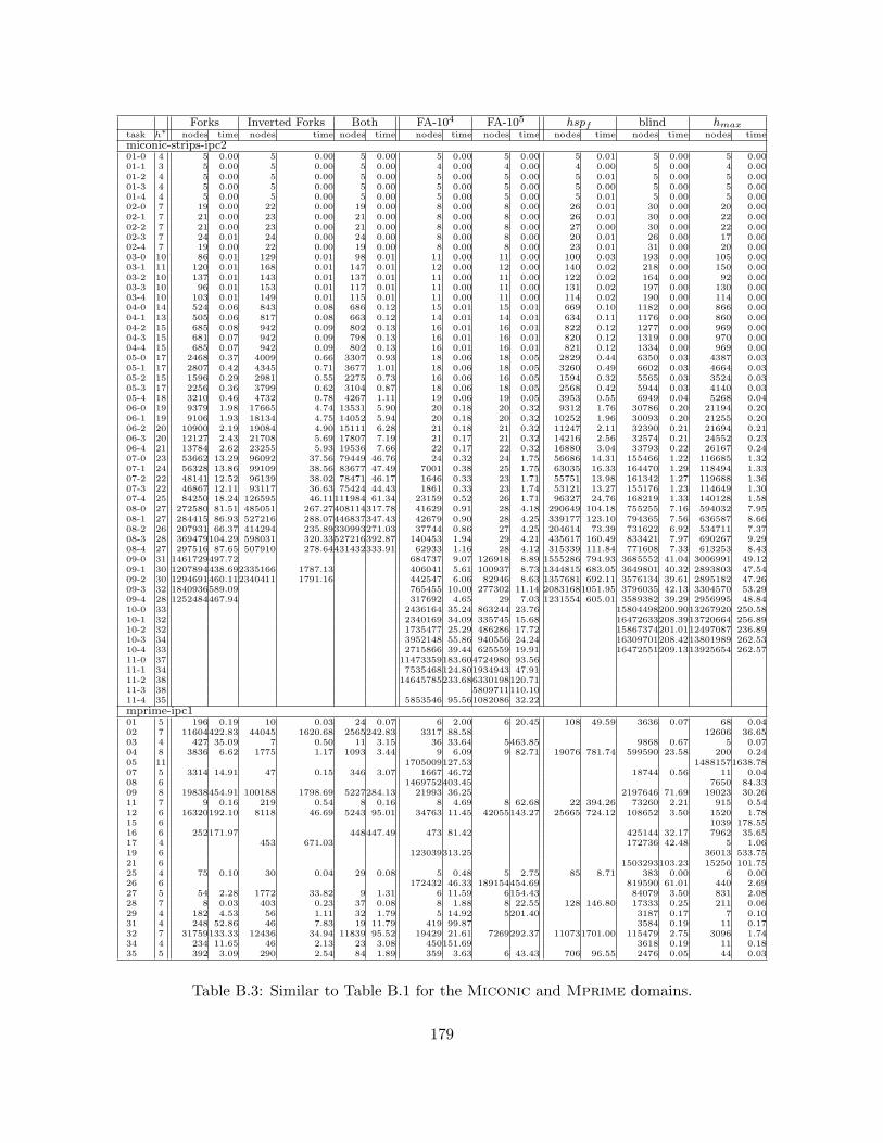
Forks Inverted Forks Both FA-104 FA-105 hspf blind hmaxtask h∗ nodes time nodes time nodes time nodes time nodes time nodes time nodes time nodes time
miconic-strips-ipc201-0 4 5 0.00 5 0.00 5 0.00 5 0.00 5 0.00 5 0.01 5 0.00 5 0.0001-1 3 5 0.00 5 0.00 5 0.00 4 0.00 4 0.00 4 0.00 5 0.00 4 0.0001-2 4 5 0.00 5 0.00 5 0.00 5 0.00 5 0.00 5 0.01 5 0.00 5 0.0001-3 4 5 0.00 5 0.00 5 0.00 5 0.00 5 0.00 5 0.00 5 0.00 5 0.0001-4 4 5 0.00 5 0.00 5 0.00 5 0.00 5 0.00 5 0.01 5 0.00 5 0.0002-0 7 19 0.00 22 0.00 19 0.00 8 0.00 8 0.00 26 0.01 30 0.00 20 0.0002-1 7 21 0.00 23 0.00 21 0.00 8 0.00 8 0.00 26 0.01 30 0.00 22 0.0002-2 7 21 0.00 23 0.00 21 0.00 8 0.00 8 0.00 27 0.00 30 0.00 22 0.0002-3 7 24 0.01 24 0.00 24 0.00 8 0.00 8 0.00 20 0.01 26 0.00 17 0.0002-4 7 19 0.00 22 0.00 19 0.00 8 0.00 8 0.00 23 0.01 31 0.00 20 0.0003-0 10 86 0.01 129 0.01 98 0.01 11 0.00 11 0.00 100 0.03 193 0.00 105 0.0003-1 11 120 0.01 168 0.01 147 0.01 12 0.00 12 0.00 140 0.02 218 0.00 150 0.0003-2 10 137 0.01 143 0.01 137 0.01 11 0.00 11 0.00 122 0.02 164 0.00 92 0.0003-3 10 96 0.01 153 0.01 117 0.01 11 0.00 11 0.00 131 0.02 197 0.00 130 0.0003-4 10 103 0.01 149 0.01 115 0.01 11 0.00 11 0.00 114 0.02 190 0.00 114 0.0004-0 14 524 0.06 843 0.08 686 0.12 15 0.01 15 0.01 669 0.10 1182 0.00 866 0.0004-1 13 505 0.06 817 0.08 663 0.12 14 0.01 14 0.01 634 0.11 1176 0.00 860 0.0004-2 15 685 0.08 942 0.09 802 0.13 16 0.01 16 0.01 822 0.12 1277 0.00 969 0.0004-3 15 681 0.07 942 0.09 798 0.13 16 0.01 16 0.01 820 0.12 1319 0.00 970 0.0004-4 15 685 0.07 942 0.09 802 0.13 16 0.01 16 0.01 821 0.12 1334 0.00 969 0.0005-0 17 2468 0.37 4009 0.66 3307 0.93 18 0.06 18 0.05 2829 0.44 6350 0.03 4387 0.0305-1 17 2807 0.42 4345 0.71 3677 1.01 18 0.06 18 0.05 3260 0.49 6602 0.03 4664 0.0305-2 15 1596 0.29 2981 0.55 2275 0.73 16 0.06 16 0.05 1594 0.32 5565 0.03 3524 0.0305-3 17 2256 0.36 3799 0.62 3104 0.87 18 0.06 18 0.05 2568 0.42 5944 0.03 4140 0.0305-4 18 3210 0.46 4732 0.78 4267 1.11 19 0.06 19 0.05 3953 0.55 6949 0.04 5268 0.0406-0 19 9379 1.98 17665 4.74 13531 5.90 20 0.18 20 0.32 9312 1.76 30786 0.20 21194 0.2006-1 19 9106 1.93 18134 4.75 14052 5.94 20 0.18 20 0.32 10252 1.96 30093 0.20 21255 0.2006-2 20 10900 2.19 19084 4.90 15111 6.28 21 0.18 21 0.32 11247 2.11 32390 0.21 21694 0.2106-3 20 12127 2.43 21708 5.69 17807 7.19 21 0.17 21 0.32 14216 2.56 32574 0.21 24552 0.2306-4 21 13784 2.62 23255 5.93 19536 7.66 22 0.17 22 0.32 16880 3.04 33793 0.22 26167 0.2407-0 23 53662 13.29 96092 37.56 79449 46.76 24 0.32 24 1.75 56686 14.31 155466 1.22 116685 1.3207-1 24 56328 13.86 99109 38.56 83677 47.49 7001 0.38 25 1.75 63035 16.33 164470 1.29 118494 1.3307-2 22 48141 12.52 96139 38.02 78471 46.17 1646 0.33 23 1.71 55751 13.98 161342 1.27 119688 1.3607-3 22 46867 12.11 93117 36.63 75424 44.43 1861 0.33 23 1.74 53121 13.27 155176 1.23 114649 1.3007-4 25 84250 18.24 126595 46.11111984 61.34 23159 0.52 26 1.71 96327 24.76 168219 1.33 140128 1.5808-0 27 272580 81.51 485051 267.27408114317.78 41629 0.91 28 4.18 290649 104.18 755255 7.16 594032 7.9508-1 27 284415 86.93 527216 288.07446837347.43 42679 0.90 28 4.25 339177 123.10 794365 7.56 636587 8.6608-2 26 207931 66.37 414294 235.89330993271.03 37744 0.86 27 4.25 204614 73.39 731622 6.92 534711 7.3708-3 28 369479104.29 598031 320.33527216392.87 140453 1.94 29 4.21 435617 160.49 833421 7.97 690267 9.2908-4 27 297516 87.65 507910 278.64431432333.91 62933 1.16 28 4.12 315339 111.84 771608 7.33 613253 8.4309-0 31 1461729497.72 684737 9.07 126918 8.89 1555286 794.93 3685552 41.04 3006991 49.1209-1 30 1207894438.692335166 1787.13 406041 5.61 100937 8.73 1344815 683.05 3649801 40.32 2893803 47.5409-2 30 1294691460.112340411 1791.16 442547 6.06 82946 8.63 1357681 692.11 3576134 39.61 2895182 47.2609-3 32 1840936589.09 765455 10.00 277302 11.14 20831681051.95 3796035 42.13 3304570 53.2909-4 28 1252484467.94 317692 4.65 29 7.03 1231554 605.01 3589382 39.29 2956995 48.8410-0 33 2436164 35.24 863244 23.76 15804498200.9013267920 250.5810-1 32 2340169 34.09 335745 15.68 16472633208.3913720664 256.8910-2 32 1735477 25.29 486286 17.72 15867374201.0112497087 236.8910-3 34 3952148 55.86 940556 24.24 16309701208.4213801989 262.5310-4 33 2715866 39.44 625559 19.91 16472551209.1313925654 262.5711-0 37 11473359183.604724980 93.5611-1 34 7535468124.801934943 47.9111-2 38 14645785233.686330198120.7111-3 38 5809711110.1011-4 35 5853546 95.561082086 32.22
mprime-ipc101 5 196 0.19 10 0.03 24 0.07 6 2.00 6 20.45 108 49.59 3636 0.07 68 0.0402 7 11604422.83 44045 1620.68 2565242.83 3317 88.58 12606 36.6503 4 427 35.09 7 0.50 11 3.15 36 33.64 5463.85 9868 0.67 5 0.0704 8 3836 6.62 1775 1.17 1093 3.44 9 6.09 9 82.71 19076 781.74 599590 23.58 200 0.2405 11 1705009127.53 14881571638.7807 5 3314 14.91 47 0.15 346 3.07 1667 46.72 18744 0.56 11 0.0408 6 1469752403.45 7650 84.3309 8 19838454.91 100188 1798.69 5227284.13 21993 36.25 2197646 71.69 19023 30.2611 7 9 0.16 219 0.54 8 0.16 8 4.69 8 62.68 22 394.26 73260 2.21 915 0.5412 6 16320192.10 8118 46.69 5243 95.01 34763 11.45 42055143.27 25665 724.12 108652 3.50 1520 1.7815 6 1039 178.5516 6 252171.97 448447.49 473 81.42 425144 32.17 7962 35.6517 4 453 671.03 172736 42.48 5 1.0619 6 123039313.25 36013 533.7521 6 1503293103.23 15250 101.7525 4 75 0.10 30 0.04 29 0.08 5 0.48 5 2.75 85 8.71 383 0.00 6 0.0026 6 172432 46.33 189154454.69 819590 61.01 440 2.6927 5 54 2.28 1772 33.82 9 1.31 6 11.59 6154.43 84079 3.50 831 2.0828 7 8 0.03 403 0.23 37 0.08 8 1.88 8 22.55 128 146.80 17333 0.25 211 0.0629 4 182 4.53 56 1.11 32 1.79 5 14.92 5201.40 3187 0.17 7 0.1031 4 248 52.86 46 7.83 19 11.79 419 99.87 3584 0.19 11 0.1732 7 31759133.33 12436 34.94 11839 95.52 19429 21.61 7269292.37 110731701.00 115479 2.75 3096 1.7434 4 234 11.65 46 2.13 23 3.08 450151.69 3618 0.19 11 0.1835 5 392 3.09 290 2.54 84 1.89 359 3.63 6 43.43 706 96.55 2476 0.05 44 0.03
Table B.3: Similar to Table B.1 for the Miconic and Mprime domains.
179
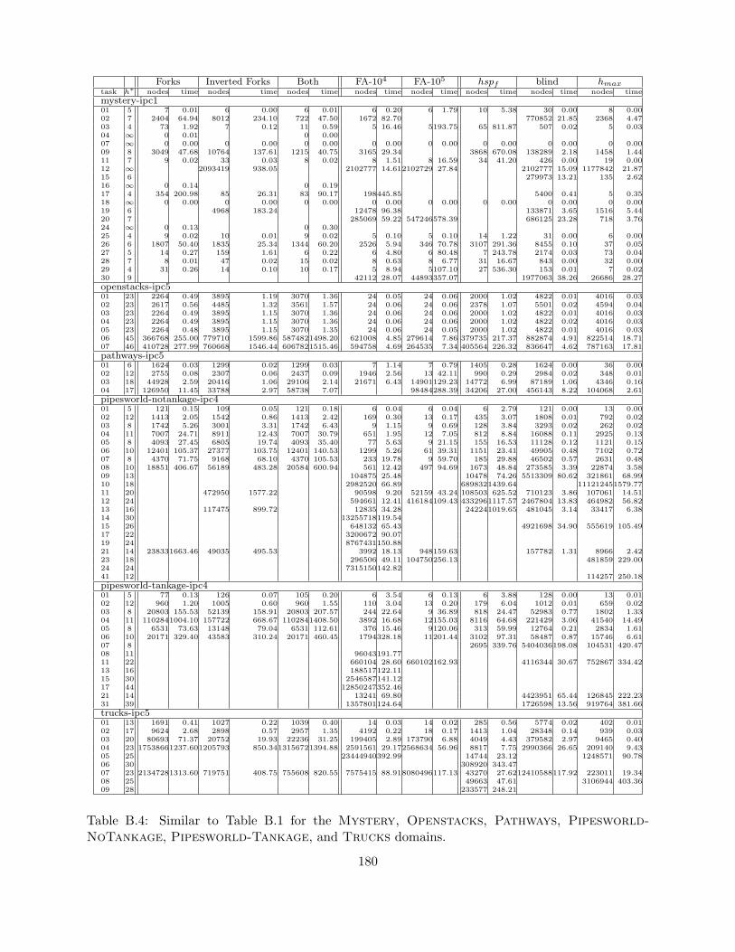
Forks Inverted Forks Both FA-104 FA-105 hspf blind hmaxtask h∗ nodes time nodes time nodes time nodes time nodes time nodes time nodes time nodes time
mystery-ipc101 5 7 0.01 6 0.00 6 0.01 6 0.20 6 1.79 10 5.38 30 0.00 8 0.0002 7 2404 64.94 8012 234.10 722 47.50 1672 82.70 770852 21.85 2368 4.4703 4 73 1.92 7 0.12 11 0.59 5 16.46 5193.75 65 811.87 507 0.02 5 0.0304 ∞ 0 0.01 0 0.0007 ∞ 0 0.00 0 0.00 0 0.00 0 0.00 0 0.00 0 0.00 0 0.00 0 0.0009 8 3049 47.68 10764 137.61 1215 40.75 3165 29.34 3868 670.08 138289 2.18 1458 1.4411 7 9 0.02 33 0.03 8 0.02 8 1.51 8 16.59 34 41.20 426 0.00 19 0.0012 ∞ 2093419 938.05 2102777 14.612102729 27.84 2102777 15.09 1177842 21.8715 6 279973 13.21 135 2.6216 ∞ 0 0.14 0 0.1917 4 354 200.98 85 26.31 83 90.17 198445.85 5400 0.41 5 0.3518 ∞ 0 0.00 0 0.00 0 0.00 0 0.00 0 0.00 0 0.00 0 0.00 0 0.0019 6 4968 183.24 12478 96.38 133871 3.65 1516 5.4420 7 285069 59.22 547246578.39 686125 23.28 718 3.7624 ∞ 0 0.13 0 0.3025 4 9 0.02 10 0.01 9 0.02 5 0.10 5 0.10 14 1.22 31 0.00 6 0.0026 6 1807 50.40 1835 25.34 1344 60.20 2526 5.94 346 70.78 3107 291.36 8455 0.10 37 0.0527 5 14 0.27 159 1.61 6 0.22 6 4.80 6 80.48 7 243.78 2174 0.03 73 0.0428 7 8 0.01 47 0.02 15 0.02 8 0.63 8 6.77 31 16.67 843 0.00 32 0.0029 4 31 0.26 14 0.10 10 0.17 5 8.94 5107.10 27 536.30 153 0.01 7 0.0230 9 42112 28.07 44893357.07 1977063 38.26 26686 28.27
openstacks-ipc501 23 2264 0.49 3895 1.19 3070 1.36 24 0.05 24 0.06 2000 1.02 4822 0.01 4016 0.0302 23 2617 0.56 4485 1.32 3561 1.57 24 0.06 24 0.06 2378 1.07 5501 0.02 4594 0.0403 23 2264 0.49 3895 1.15 3070 1.36 24 0.06 24 0.06 2000 1.02 4822 0.01 4016 0.0304 23 2264 0.49 3895 1.15 3070 1.36 24 0.06 24 0.06 2000 1.02 4822 0.02 4016 0.0305 23 2264 0.48 3895 1.15 3070 1.35 24 0.06 24 0.05 2000 1.02 4822 0.01 4016 0.0306 45 366768 255.00 779710 1599.86 5874821498.20 621008 4.85 279614 7.86 379735 217.37 882874 4.91 822514 18.7107 46 410728 277.99 760668 1546.44 6067821515.46 594758 4.69 264535 7.34 405564 226.32 836647 4.62 787163 17.81
pathways-ipc501 6 1624 0.03 1299 0.02 1299 0.03 7 1.14 7 0.79 1405 0.28 1624 0.00 36 0.0002 12 2755 0.08 2307 0.06 2437 0.09 1946 2.56 13 42.11 990 0.29 2984 0.02 348 0.0103 18 44928 2.59 20416 1.06 29106 2.14 21671 6.43 14901129.23 14772 6.99 87189 1.06 4346 0.1604 17 126950 11.45 33788 2.97 58738 7.07 98484288.39 34206 27.00 456143 8.22 104068 2.61
pipesworld-notankage-ipc401 5 121 0.15 109 0.05 121 0.18 6 0.04 6 0.04 6 2.79 121 0.00 13 0.0002 12 1413 2.05 1542 0.86 1413 2.42 169 0.30 13 0.17 435 3.07 1808 0.01 792 0.0203 8 1742 5.26 3001 3.31 1742 6.43 9 1.15 9 0.69 128 3.84 3293 0.02 262 0.0204 11 7007 24.71 8911 12.43 7007 30.79 651 1.95 12 7.05 812 8.84 16088 0.11 2925 0.1305 8 4093 27.45 6805 19.74 4093 35.40 77 5.63 9 21.15 155 16.53 11128 0.12 1121 0.1506 10 12401 105.37 27377 103.75 12401 140.53 1299 5.26 61 39.31 1151 23.41 49905 0.48 7102 0.7207 8 4370 71.75 9168 68.10 4370 105.53 233 19.78 9 59.70 185 29.88 46502 0.57 2631 0.4808 10 18851 406.67 56189 483.28 20584 600.94 561 12.42 497 94.69 1673 48.84 273585 3.39 22874 3.5809 13 104875 25.48 10478 74.26 5513309 80.62 321861 68.9910 18 2982520 66.89 6898321439.64 111212451579.7711 20 472950 1577.22 90598 9.20 52159 43.24 108503 625.52 710123 3.86 107061 14.5112 24 594661 12.41 416184109.43 4332961117.57 2467804 13.83 464982 56.8213 16 117475 899.72 12835 34.28 242241019.65 481045 3.14 33417 6.3814 30 13255718119.5415 26 648132 65.43 4921698 34.90 555619 105.4917 22 3200672 90.0719 24 8767431150.8821 14 238331663.46 49035 495.53 3992 18.13 948159.63 157782 1.31 8966 2.4223 18 296506 49.11 104750256.13 481859 229.0024 24 7315150142.8241 12 114257 250.18
pipesworld-tankage-ipc401 5 77 0.13 126 0.07 105 0.20 6 3.54 6 0.13 6 3.88 128 0.00 13 0.0102 12 960 1.20 1005 0.60 960 1.55 110 3.04 13 0.20 179 6.04 1012 0.01 659 0.0203 8 20803 155.53 52139 158.91 20803 207.57 244 22.64 9 36.89 818 24.47 52983 0.77 1802 1.3304 11 1102841004.10 157722 668.67 1102841408.50 3892 16.68 12155.03 8116 64.68 221429 3.06 41540 14.4905 8 6531 73.63 13148 79.04 6531 112.61 376 15.46 9120.06 313 59.99 12764 0.21 2834 1.6106 10 20171 329.40 43583 310.24 20171 460.45 1794328.18 11201.44 3102 97.31 58487 0.87 15746 6.6107 8 2695 339.76 5404036198.08 104531 420.4708 11 96043191.7711 22 660104 28.60 660102162.93 4116344 30.67 752867 334.4213 16 188517122.1115 30 2546587141.1217 44 12850247352.4621 14 13241 69.80 4423951 65.44 126845 222.2331 39 1357801124.64 1726598 13.56 919764 381.66
trucks-ipc501 13 1691 0.41 1027 0.22 1039 0.40 14 0.03 14 0.02 285 0.56 5774 0.02 402 0.0102 17 9624 2.68 2898 0.57 2957 1.35 4192 0.22 18 0.17 1413 1.04 28348 0.14 939 0.0303 20 80693 71.37 20752 19.93 22236 31.25 199405 2.89 173790 6.88 4049 4.43 379582 2.97 9465 0.4004 23 17538661237.601205793 850.3413156721394.88 2591561 29.172568634 56.96 8817 7.75 2990366 26.65 209140 9.4305 25 23444940392.99 14744 23.12 1248571 90.7806 30 308920 343.4707 23 21347281313.60 719751 408.75 755608 820.55 7575415 88.918080496117.13 43270 27.6212410588117.92 223011 19.3408 25 49663 47.61 3106944 403.3609 28 233577 248.21
Table B.4: Similar to Table B.1 for the Mystery, Openstacks, Pathways, Pipesworld-NoTankage, Pipesworld-Tankage, and Trucks domains.
180
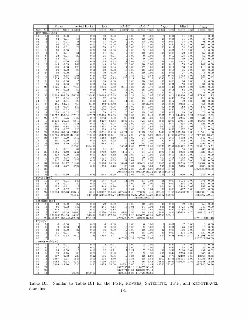
Forks Inverted Forks Both FA-104 FA-105 hspf blind hmaxtask h∗ nodes time nodes time nodes time nodes time nodes time nodes time nodes time nodes time
psr-small-ipc401 8 10 0.00 10 0.00 10 0.00 9 0.00 9 0.00 9 0.01 11 0.00 9 0.0002 11 52 0.01 55 0.00 52 0.01 12 0.00 12 0.00 20 0.08 71 0.00 47 0.0003 11 31 0.01 31 0.00 31 0.00 12 0.00 12 0.00 20 0.04 33 0.00 28 0.0004 10 66 0.04 91 0.03 73 0.06 11 0.00 11 0.00 12 0.34 332 0.00 102 0.0005 11 75 0.01 79 0.01 75 0.02 12 0.00 12 0.00 23 0.11 154 0.00 69 0.0006 8 10 0.00 10 0.00 10 0.00 9 0.00 9 0.00 9 0.01 11 0.00 9 0.0007 11 61 0.01 61 0.00 61 0.01 12 0.00 12 0.00 26 0.09 122 0.00 62 0.0008 8 24 0.01 29 0.00 25 0.01 9 0.00 9 0.00 9 0.12 128 0.00 52 0.0009 8 18 0.01 19 0.00 18 0.00 9 0.00 9 0.00 9 0.06 49 0.00 20 0.0010 7 131 0.20 183 0.18 155 0.32 8 0.04 8 0.04 18 1.04 1358 0.00 376 0.0111 19 149 0.03 149 0.02 149 0.04 20 0.00 20 0.00 96 0.19 153 0.00 142 0.0012 16 120 0.03 123 0.02 120 0.04 17 0.00 17 0.00 40 0.17 153 0.00 113 0.0013 15 90 0.02 90 0.01 90 0.02 16 0.00 16 0.00 59 0.16 95 0.00 86 0.0014 9 19 0.00 19 0.00 19 0.00 10 0.00 10 0.00 13 0.06 27 0.00 18 0.0015 10 1200 6.55 708 6.25 769 9.91 11 0.46 11 2.58 356 18.99 3562 0.02 324 0.0216 25 2328 0.65 2158 0.34 2176 0.85 975 0.11 26 0.12 2287 1.34 2742 0.01 1876 0.0117 9 15 0.00 15 0.00 15 0.00 10 0.00 10 0.00 13 0.03 16 0.00 14 0.0018 12 85 0.03 90 0.01 85 0.03 13 0.00 13 0.00 29 0.21 158 0.00 91 0.0019 25 8025 4.31 7856 2.19 7876 5.80 2910 0.27 26 0.77 6338 4.46 9009 0.04 6925 0.0820 17 80 0.02 80 0.01 80 0.02 18 0.00 18 0.00 52 0.18 84 0.00 75 0.0021 10 28 0.01 28 0.00 28 0.01 11 0.00 11 0.00 21 0.12 42 0.00 31 0.0022 33 163299 405.65 176058 245.42 168685 617.45 34 0.28 34 0.87 22315 8.16 189516 0.67 177138 1.4323 12 77 0.04 93 0.03 77 0.06 13 0.00 13 0.01 30 0.43 200 0.00 116 0.0024 10 28 0.01 28 0.00 28 0.01 11 0.00 11 0.00 21 0.12 42 0.00 31 0.0025 9 485 84.24 463 145.38 482 213.42 10 5.42 10 37.93 28 780.38 8913 0.12 854 0.1826 17 144 0.05 150 0.03 146 0.06 18 0.00 18 0.00 52 0.28 182 0.00 142 0.0027 21 616 0.33 675 0.21 650 0.49 22 0.01 22 0.01 179 0.85 773 0.00 616 0.0028 14 79 0.02 79 0.01 79 0.02 15 0.00 15 0.00 49 0.29 95 0.00 79 0.0029 21 142772 436.34 187319 307.77 159325 709.89 22 0.39 22 1.43 3337 7.12 244499 1.27 192459 2.3230 22 1791 1.25 1982 0.80 1883 1.90 23 0.01 23 0.02 393 1.35 2295 0.01 1834 0.0131 19 11278 25.93 6810 38.66 8297 53.43 2647 0.89 723 6.55 7530 32.97 53911 0.25 16766 0.3632 24 431 0.17 431 0.10 431 0.25 25 0.00 25 0.00 352 0.74 435 0.00 424 0.0033 21 1480 0.84 1436 0.30 1391 1.00 446 0.26 22 0.63 947 2.29 2291 0.01 1073 0.0134 21 223 0.07 223 0.04 223 0.09 22 0.00 22 0.00 158 0.50 227 0.00 216 0.0035 22 65965 160.36 63186 39.55 68281 199.30 24021 0.83 11113 6.36 7448 8.27 165170 0.63 61548 1.0636 22 571766 392.49 371834 786.06 4584021094.61 48350 2.98 2783 14.07 188564 111.991669788 9.44 717884 18.2737 23 1307 1.29 1417 0.95 1363 2.10 24 0.02 24 0.01 277 2.10 1532 0.00 1342 0.0138 13 301 0.20 372 0.15 326 0.32 14 0.01 14 0.01 33 0.74 562 0.00 357 0.0039 23 2486 2.49 2942 1.64 2682 3.91 24 0.08 24 0.07 146 1.78 4103 0.01 2597 0.0240 20 182608 1384.90 38837 1.88 7767 12.86 23371 87.911036992 6.74 229210 9.5141 10 31 0.01 34 0.00 31 0.01 11 0.00 11 0.00 21 0.16 54 0.00 35 0.0042 30 1855 0.50 1747 0.17 1739 0.59 1117 0.18 31 0.18 1773 1.29 1908 0.01 1636 0.0143 20 328 0.09 328 0.05 328 0.12 21 0.00 21 0.00 256 0.50 333 0.00 315 0.0044 19 2990 3.25 3430 2.30 3121 5.24 20 0.05 20 0.05 407 2.18 4142 0.01 3235 0.0245 20 347 0.16 376 0.11 359 0.25 21 0.01 21 0.00 121 0.74 434 0.00 358 0.0046 34 60888 51.77 61842 21.14 61563 68.33 36941 0.67 32582 4.05 19865 6.91 80785 0.25 65984 0.6347 27 4104 5.27 4522 3.93 4284 8.70 28 0.04 28 0.04 515 2.32 5075 0.01 4406 0.0248 37 129627 2.37 2500 11.08 200559 101.21 19020089286.0249 47 204836815.84 594399 23.32 27728751408.6450 23 637 0.39 659 0.26 645 0.60 24 0.02 24 0.02 390 1.40 690 0.00 642 0.00
rovers-ipc501 10 147 0.01 147 0.01 147 0.02 11 0.03 11 0.03 48 0.07 1104 0.00 283 0.0002 8 44 0.01 44 0.01 44 0.01 9 0.00 9 0.00 16 0.03 254 0.00 129 0.0003 11 672 0.11 419 0.05 448 0.10 12 0.11 12 0.12 804 0.16 3543 0.02 757 0.0004 8 47 0.02 20 0.00 24 0.01 9 0.04 9 0.04 58 0.08 897 0.00 223 0.0005 22 808084 237.13 410712 123.64 522937 231.28 61726711.48 375808 18.46 298400 101.658559690126.19 4318309 81.5307 18 741649 517.1816822451780.27 328088451.022212903 59.20 1459792 866.93 9618062199.9112 19 5187273166.77
satellite-ipc401 9 24 0.00 32 0.00 29 0.00 10 0.00 10 0.00 46 0.06 89 0.00 59 0.0002 13 86 0.02 337 0.10 241 0.13 14 0.01 14 0.01 646 0.21 1728 0.01 940 0.0003 11 2249 1.24 656 0.53 728 0.82 12 0.56 12 0.64 1945 0.93 15185 0.17 6822 0.1104 17 9817 10.65 14860 24.90 11250 26.18 4152 0.99 18 4.43 15890 9.50 345663 4.70 180815 3.3705 15 2795691251.83 46453 515.80 61692 877.26 81972 7.26 148667 69.28 267513 565.1806 20 1496577 968.241572327 1721.87 276922974.73 307962 32.52 10751017371.43
tpp-ipc501 5 6 0.00 6 0.00 6 0.00 6 0.00 6 0.00 6 0.01 7 0.00 6 0.0002 8 9 0.00 11 0.00 9 0.00 9 0.00 9 0.00 9 0.01 26 0.00 16 0.0003 11 12 0.00 27 0.00 16 0.00 12 0.00 12 0.00 12 0.03 116 0.00 83 0.0004 14 15 0.01 78 0.01 47 0.01 15 0.01 15 0.00 15 0.07 494 0.00 430 0.0005 19 623 0.52 5110 1.36 1455 1.21 20 0.36 20 0.77 624 0.48 24698 0.12 17398 0.1506 25 94705914.22 74798 23.97 9267024216.69
zenotravel-ipc301 1 2 0.01 2 0.00 2 0.01 2 0.00 2 0.00 2 0.45 2 0.00 2 0.0002 6 17 0.02 18 0.02 17 0.02 7 0.00 7 0.00 9 0.46 58 0.00 22 0.0003 6 28 0.08 18 0.12 12 0.11 7 0.21 7 0.90 40 3.42 5160 0.04 492 0.0204 8 99 0.15 88 0.26 81 0.30 9 0.20 9 0.89 215 3.44 5256 0.03 665 0.0105 11 177 0.32 220 0.22 136 0.36 12 0.25 12 1.90 422 7.70 82289 0.63 12466 0.3306 11 2287 5.51 1144 2.00 504 2.40 12 0.38 12 3.54 1957 11.81 596531 5.90 85931 2.4707 15 5088 9.63 4234 5.56 4199 10.58 16 0.38 16 3.48 34890 30.36 405626 3.56 115348 2.6008 11 3268 43.96 1026 8.92 1655 30.06 14354 2.00 12 14.48 83533 292.05 687846 50.7609 21 251703551.18 611457 30.4710 22 132287134.84 137872 25.4411 14 76904 1090.67 31003011.28 110726 26.65
Table B.5: Similar to Table B.1 for the PSR, Rovers, Satellite, TPP, and Zenotraveldomains. 181
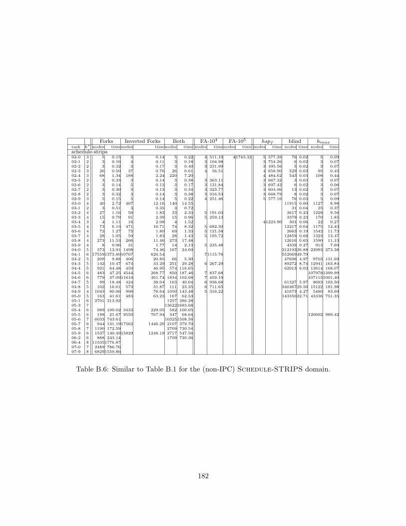
Forks Inverted Forks Both FA-104 FA-105 hspf blind hmaxtask h∗ nodes timenodes timenodes time nodes timenodes time nodes time nodes time nodes time
schedule-strips02-0 3 5 0.15 5 0.14 5 0.22 4 511.10 41743.32 5 577.39 76 0.02 5 0.0902-1 2 3 0.16 4 0.11 3 0.18 3 104.98 3 754.26 6 0.02 3 0.0702-2 2 3 0.32 3 0.17 3 0.40 3 231.99 3 495.56 5 0.02 3 0.0702-3 3 26 0.50 37 0.76 26 0.61 4 56.51 4 658.90 529 0.03 95 0.4502-4 3 68 1.34 188 2.24 220 7.20 4 484.62 543 0.03 108 0.4402-5 2 3 0.33 3 0.14 3 0.38 3 363.11 3 667.32 3 0.03 3 0.0702-6 2 3 0.14 5 0.12 3 0.17 3 121.84 3 697.42 6 0.02 3 0.0602-7 2 3 0.30 3 0.13 3 0.34 3 323.77 3 604.06 13 0.02 3 0.0702-8 2 3 0.32 3 0.14 3 0.38 3 316.53 3 668.79 8 0.02 3 0.0702-9 3 5 0.15 5 0.14 5 0.22 4 251.46 5 577.16 76 0.03 5 0.0903-0 4 40 2.72 407 12.16 140 14.55 11915 0.60 1127 8.9803-1 2 3 0.51 3 0.35 3 0.72 31 0.04 25 0.3703-2 4 27 1.16 50 1.83 33 2.33 5 191.03 3617 0.23 1228 9.5603-3 4 15 0.79 91 2.39 15 0.96 5 259.13 3379 0.23 170 1.8503-4 3 4 1.11 16 2.08 4 1.52 41223.90 301 0.06 22 0.2703-5 4 73 6.13 471 16.71 74 8.32 5 682.30 12217 0.64 1175 12.4303-6 4 72 1.27 75 1.80 69 1.33 5 121.58 2663 0.19 1542 11.7303-7 4 28 1.05 50 1.83 28 1.43 5 195.72 12859 0.68 1323 13.4703-8 4 273 11.53 266 11.46 273 17.48 12616 0.65 1590 11.1303-9 4 8 0.96 31 1.77 14 2.13 5 235.48 4339 0.27 913 7.6904-0 5 373 13.91 1498 74.46 167 24.60 31219326.88 22993 273.3804-1 6 175591373.8010707 626.54 71115.76 55206949.7904-2 5 209 9.88 406 20.85 66 5.30 47696 4.97 9703 131.6904-3 5 142 10.47 674 33.29 251 29.28 6 267.29 89272 8.74 12941 163.8404-4 5 921 64.48 450 46.95 574 116.65 62013 6.03 13614 168.0704-5 6 483 47.25 4544 268.77 850 187.46 7 837.68 1079781399.9904-6 6 779 27.0911610 361.74 1834 102.68 7 459.19 1071151001.4004-7 5 99 18.48 424 38.04 163 40.04 6 936.68 61327 5.97 8683 103.5004-8 5 102 16.01 573 31.87 111 23.35 6 711.65 34046729.56 15122 181.9804-9 4 1043 80.06 996 76.64 1050 143.48 5 316.22 41673 4.27 5480 83.6905-0 5 163 41.61 483 63.23 167 62.53 14335022.71 43336 751.3505-1 6 2701 213.92 1257 286.2805-3 7 136221693.6805-4 6 989 100.02 3433 229.05 582 100.0505-5 6 198 21.67 9550 767.94 347 68.64 120602 989.4205-6 7 6033 743.61 103251508.5605-7 6 944 131.1917562 1446.20 2107 379.7005-8 7 1190 172.59 2709 730.5405-9 6 1537 140.4915829 1248.19 2717 547.5606-2 6 888 243.14 1709 730.3606-4 8 115351776.8707-0 7 2489 786.7607-9 8 68291559.86
Table B.6: Similar to Table B.1 for the (non-IPC) Schedule-STRIPS domain.
182
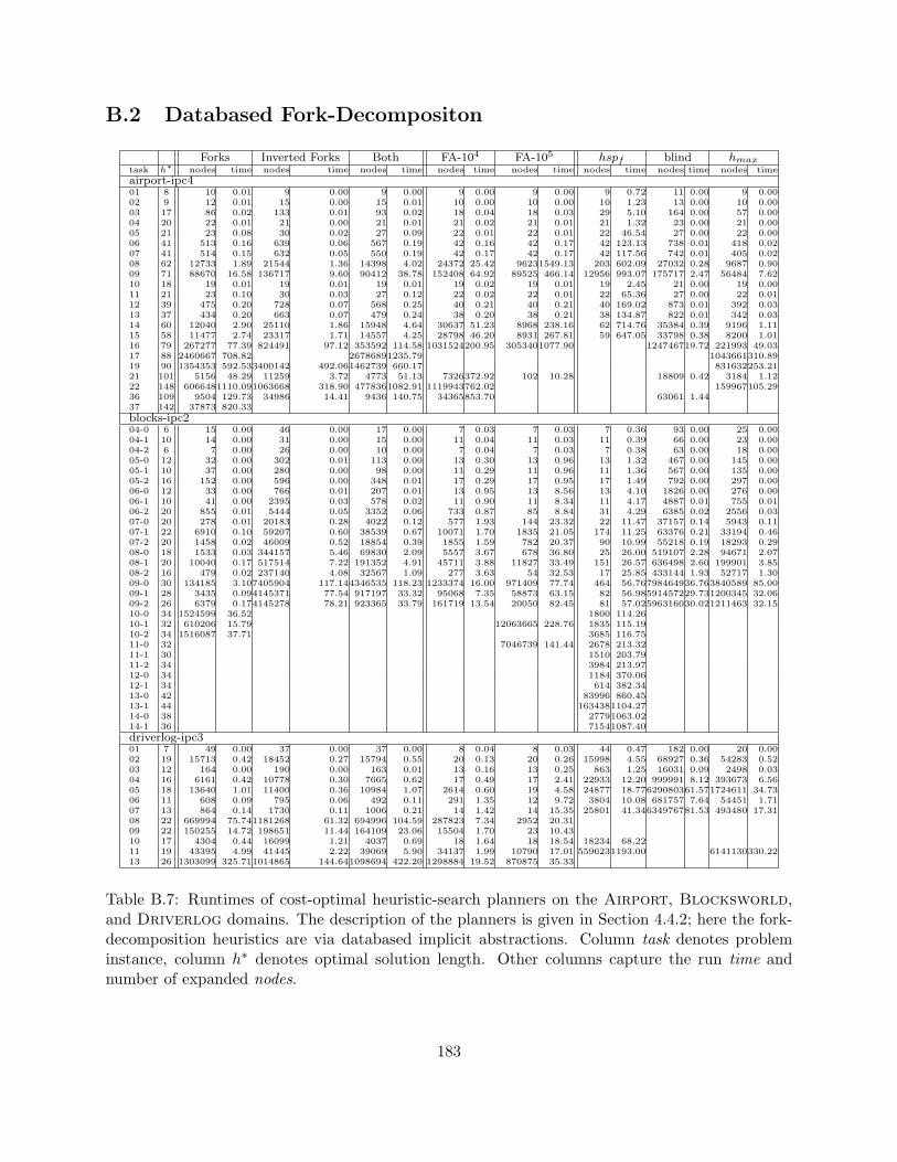
B.2 Databased Fork-Decompositon
Forks Inverted Forks Both FA-104 FA-105 hspf blind hmaxtask h∗ nodes time nodes time nodes time nodes time nodes time nodes time nodes time nodes time
airport-ipc401 8 10 0.01 9 0.00 9 0.00 9 0.00 9 0.00 9 0.72 11 0.00 9 0.0002 9 12 0.01 15 0.00 15 0.01 10 0.00 10 0.00 10 1.23 13 0.00 10 0.0003 17 86 0.02 133 0.01 93 0.02 18 0.04 18 0.03 29 5.10 164 0.00 57 0.0004 20 22 0.01 21 0.00 21 0.01 21 0.02 21 0.01 21 1.32 23 0.00 21 0.0005 21 23 0.08 30 0.02 27 0.09 22 0.01 22 0.01 22 46.54 27 0.00 22 0.0006 41 513 0.16 639 0.06 567 0.19 42 0.16 42 0.17 42 123.13 738 0.01 418 0.0207 41 514 0.15 632 0.05 550 0.19 42 0.17 42 0.17 42 117.56 742 0.01 405 0.0208 62 12733 1.89 21544 1.36 14398 4.02 24372 25.42 96231549.13 203 602.09 27032 0.28 9687 0.9009 71 88670 16.58 136717 9.60 90412 38.78 152408 64.92 89525 466.14 12956 993.07 175717 2.47 56484 7.6210 18 19 0.01 19 0.01 19 0.01 19 0.02 19 0.01 19 2.45 21 0.00 19 0.0011 21 23 0.10 30 0.03 27 0.12 22 0.02 22 0.01 22 65.36 27 0.00 22 0.0112 39 475 0.20 728 0.07 568 0.25 40 0.21 40 0.21 40 169.02 873 0.01 392 0.0313 37 434 0.20 663 0.07 479 0.24 38 0.20 38 0.21 38 134.87 822 0.01 342 0.0314 60 12040 2.90 25110 1.86 15948 4.64 30637 51.23 8968 238.16 62 714.76 35384 0.39 9196 1.1115 58 11477 2.74 23317 1.71 14557 4.25 28798 46.20 8931 267.81 59 647.05 33798 0.38 8200 1.0116 79 267277 77.39 824491 97.12 353592 114.58 1031524200.95 3053401077.90 124746719.72 221993 49.0317 88 2460667 708.82 26786891235.79 1043661310.8919 90 1354353 592.533400142 492.061462739 660.17 831632253.2121 101 5156 48.29 11259 3.72 4773 51.13 7326372.92 102 10.28 18809 0.42 3184 1.1222 148 6066481110.091063668 318.90 4778361082.91 1119943762.02 159967105.2936 109 9504 129.73 34986 14.41 9436 140.75 34365853.70 63061 1.4437 142 37873 820.33
blocks-ipc204-0 6 15 0.00 46 0.00 17 0.00 7 0.03 7 0.03 7 0.36 93 0.00 25 0.0004-1 10 14 0.00 31 0.00 15 0.00 11 0.04 11 0.03 11 0.39 66 0.00 23 0.0004-2 6 7 0.00 26 0.00 10 0.00 7 0.04 7 0.03 7 0.38 63 0.00 18 0.0005-0 12 32 0.00 302 0.01 113 0.00 13 0.30 13 0.96 13 1.32 467 0.00 145 0.0005-1 10 37 0.00 280 0.00 98 0.00 11 0.29 11 0.96 11 1.36 567 0.00 135 0.0005-2 16 152 0.00 596 0.00 348 0.01 17 0.29 17 0.95 17 1.49 792 0.00 297 0.0006-0 12 33 0.00 766 0.01 207 0.01 13 0.95 13 8.56 13 4.10 1826 0.00 276 0.0006-1 10 41 0.00 2395 0.03 578 0.02 11 0.90 11 8.34 11 4.17 4887 0.01 755 0.0106-2 20 855 0.01 5444 0.05 3352 0.06 733 0.87 85 8.84 31 4.29 6385 0.02 2556 0.0307-0 20 278 0.01 20183 0.28 4022 0.12 577 1.93 144 23.32 22 11.47 37157 0.14 5943 0.1107-1 22 6910 0.10 59207 0.60 38539 0.67 10071 1.70 1835 21.05 174 11.25 63376 0.21 33194 0.4607-2 20 1458 0.02 46009 0.52 18854 0.39 1855 1.59 782 20.37 90 10.99 55218 0.19 18293 0.2908-0 18 1533 0.03 344157 5.46 69830 2.09 5557 3.67 678 36.80 25 26.00 519107 2.28 94671 2.0708-1 20 10040 0.17 517514 7.22 191352 4.91 45711 3.88 11827 33.49 151 26.57 636498 2.60 199901 3.8508-2 16 479 0.02 237140 4.08 32567 1.09 277 3.63 54 32.53 17 25.85 433144 1.93 52717 1.3009-0 30 134185 3.107405904 117.144346535 118.23 1233374 16.00 971409 77.74 464 56.76798464936.763840589 85.0009-1 28 3435 0.094145371 77.54 917197 33.32 95068 7.35 58873 63.15 82 56.98591457229.731200345 32.0609-2 26 6379 0.174145278 78.21 923365 33.79 161719 13.54 20050 82.45 81 57.02596316030.021211463 32.1510-0 34 1524599 36.52 1800 114.2610-1 32 610206 15.79 12063665 228.76 1835 115.1910-2 34 1516087 37.71 3685 116.7511-0 32 7046739 141.44 2678 213.3211-1 30 1510 203.7911-2 34 3984 213.9712-0 34 1184 370.0612-1 34 614 382.3413-0 42 83996 860.4513-1 44 1634381104.2714-0 38 27791063.0214-1 36 71541087.40
driverlog-ipc301 7 49 0.00 37 0.00 37 0.00 8 0.04 8 0.03 44 0.47 182 0.00 20 0.0002 19 15713 0.42 18452 0.27 15794 0.55 20 0.13 20 0.26 15998 4.55 68927 0.36 54283 0.5203 12 164 0.00 190 0.00 163 0.01 13 0.16 13 0.25 863 1.25 16031 0.09 2498 0.0304 16 6161 0.42 10778 0.30 7665 0.62 17 0.49 17 2.41 22933 12.20 999991 8.12 393673 6.5605 18 13640 1.01 11400 0.36 10984 1.07 2614 0.60 19 4.58 24877 18.77629080361.571724611 34.7306 11 608 0.09 795 0.06 492 0.11 291 1.35 12 9.72 3804 10.08 681757 7.64 54451 1.7107 13 864 0.14 1730 0.11 1006 0.21 14 1.42 14 15.35 25801 41.34634976781.53 493480 17.3108 22 669994 75.741181268 61.32 694996 104.59 287823 7.34 2952 20.3109 22 150255 14.72 198651 11.44 164109 23.06 15504 1.70 23 10.4310 17 4304 0.44 16099 1.21 4037 0.69 18 1.64 18 18.54 18234 68.2211 19 43395 4.99 41445 2.22 39069 5.90 34137 1.99 10790 17.01 5596231193.00 6141130330.2213 26 1303099 325.711014865 144.641098694 422.20 1298884 19.52 870875 35.33
Table B.7: Runtimes of cost-optimal heuristic-search planners on the Airport, Blocksworld,and Driverlog domains. The description of the planners is given in Section 4.4.2; here the fork-decomposition heuristics are via databased implicit abstractions. Column task denotes probleminstance, column h∗ denotes optimal solution length. Other columns capture the run time andnumber of expanded nodes.
183
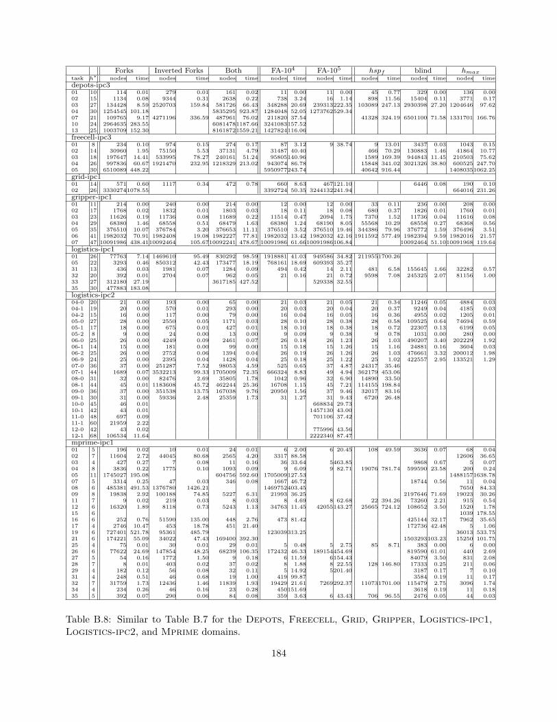
Forks Inverted Forks Both FA-104 FA-105 hspf blind hmaxtask h∗ nodes time nodes time nodes time nodes time nodes time nodes time nodes time nodes time
depots-ipc301 10 114 0.01 279 0.01 161 0.02 11 0.00 11 0.00 45 0.77 329 0.00 136 0.0002 15 1134 0.08 9344 0.31 2638 0.22 738 3.24 16 1.14 898 11.56 15404 0.11 3771 0.1703 27 134428 8.59 2520703 159.84 581726 66.43 348288 20.69 239313222.35 103089 247.13 2930398 27.20 1204646 97.6204 30 1254545 101.18 5835295 923.87 1284048 52.05 1273762529.3407 21 109765 9.17 4271196 336.59 487961 76.02 211820 37.54 41328 324.19 6501100 71.58 1331701 166.7610 24 2964635 283.55 60814781187.66 3241083157.5213 25 1003709 152.30 81618721559.21 1427824116.06
freecell-ipc301 8 234 0.10 974 0.15 274 0.17 87 3.12 9 38.74 9 13.01 3437 0.03 1043 0.1502 14 30960 1.95 75150 5.53 37131 4.79 31487 40.40 466 70.29 130883 1.46 41864 10.7703 18 197647 14.41 533995 78.27 240161 51.24 95805140.96 1589 169.39 944843 11.45 210503 75.6204 26 997836 60.67 1921470 232.95 1218329 213.02 943074 86.78 15848 341.02 3021326 38.80 600525 247.7005 30 6510089 448.22 5950977243.74 40642 916.44 14080351062.25
grid-ipc101 14 571 0.60 1117 0.34 472 0.78 660 8.63 467121.10 6446 0.08 190 0.1002 26 33302741078.55 3392724 50.35 3244132241.94 664016 231.26
gripper-ipc101 11 214 0.00 240 0.00 214 0.00 12 0.00 12 0.00 33 0.11 236 0.00 208 0.0002 17 1768 0.02 1832 0.01 1803 0.03 18 0.11 18 0.08 680 0.37 1826 0.01 1760 0.0103 23 11626 0.19 11736 0.08 11689 0.22 11514 0.47 2094 1.75 7370 1.52 11736 0.04 11616 0.0804 29 68380 1.46 68558 0.51 68479 1.63 68380 1.24 68190 8.05 55568 10.29 68558 0.27 68368 0.5605 35 376510 10.07 376784 3.20 376653 11.11 376510 3.52 376510 19.46 344386 79.96 376772 1.59 376496 3.5106 41 1982032 70.91 1982408 19.08 1982227 77.81 1982032 13.42 1982032 42.16 1911592 577.49 1982394 9.59 1982016 21.5707 47 10091986 438.4110092464 105.6710092241 478.67 10091986 61.6610091986106.84 10092464 51.1010091968 119.64
logistics-ipc101 26 77763 7.14 1469610 95.49 830292 98.59 1918881 41.03 949586 34.82 2119551700.2605 22 3293 0.46 850312 42.43 173477 18.19 768161 18.69 609393 35.2731 13 436 0.03 1981 0.07 1284 0.09 494 0.42 14 2.11 481 6.58 155645 1.66 32282 0.5732 20 392 0.01 2704 0.07 962 0.05 21 0.16 21 0.72 9598 7.08 245325 2.07 81156 1.0033 27 312180 27.19 3617185 427.52 529338 32.5535 30 477883 183.08
logistics-ipc204-0 20 21 0.00 193 0.00 65 0.00 21 0.03 21 0.05 21 0.34 11246 0.05 4884 0.0304-1 19 20 0.00 570 0.01 293 0.00 20 0.03 20 0.04 20 0.37 9249 0.04 4185 0.0304-2 15 16 0.00 117 0.00 79 0.00 16 0.04 16 0.05 16 0.36 4955 0.02 1205 0.0105-0 27 28 0.00 2550 0.05 1171 0.03 28 0.10 28 0.38 28 0.58 109525 0.64 74694 0.5905-1 17 18 0.00 675 0.01 427 0.01 18 0.10 18 0.38 18 0.72 22307 0.13 6199 0.0505-2 8 9 0.00 24 0.00 13 0.00 9 0.09 9 0.38 9 0.78 1031 0.00 280 0.0006-0 25 26 0.00 4249 0.09 2461 0.07 26 0.18 26 1.23 26 1.03 490207 3.40 202229 1.9206-1 14 15 0.00 181 0.00 99 0.00 15 0.18 15 1.26 15 1.16 24881 0.16 3604 0.0306-2 25 26 0.00 2752 0.06 1394 0.04 26 0.19 26 1.26 26 1.03 476661 3.32 200012 1.9806-9 24 25 0.00 2395 0.04 1428 0.04 25 0.18 25 1.22 25 1.02 422557 2.95 133521 1.2907-0 36 37 0.00 251287 7.52 98053 4.59 525 0.65 37 4.87 24317 35.4607-1 44 1689 0.07 3532213 99.33 1705009 72.35 666324 8.83 49 4.94 362179 453.0608-0 31 32 0.00 82476 2.69 35805 1.78 1042 0.96 32 6.90 14890 33.5008-1 44 45 0.01 1183608 45.72 462244 25.36 16708 1.15 45 7.21 114155 198.8409-0 36 37 0.00 351538 13.75 167038 9.76 20950 1.56 37 9.46 32017 83.1609-1 30 31 0.00 59336 2.48 25359 1.73 31 1.27 31 9.43 6720 26.4810-0 45 46 0.01 668834 29.7310-1 42 43 0.01 1457130 43.0011-0 48 697 0.09 701106 37.4211-1 60 21959 2.2212-0 42 43 0.02 775996 43.5612-1 68 106534 11.64 2222340 87.47
mprime-ipc101 5 196 0.02 10 0.01 24 0.01 6 2.00 6 20.45 108 49.59 3636 0.07 68 0.0402 7 11604 2.72 44045 80.68 2565 4.20 3317 88.58 12606 36.6503 4 427 0.27 7 0.08 11 0.16 36 33.64 5463.85 9868 0.67 5 0.0704 8 3836 0.22 1775 0.10 1093 0.09 9 6.09 9 82.71 19076 781.74 599590 23.58 200 0.2405 11 1745027 195.08 604756 592.60 1705009127.53 14881571638.7807 5 3314 0.25 47 0.03 346 0.08 1667 46.72 18744 0.56 11 0.0408 6 485381 491.53 1376780 1426.21 1469752403.45 7650 84.3309 8 19838 2.92 100188 74.85 5227 6.31 21993 36.25 2197646 71.69 19023 30.2611 7 9 0.02 219 0.03 8 0.03 8 4.69 8 62.68 22 394.26 73260 2.21 915 0.5412 6 16320 1.89 8118 0.73 5243 1.13 34763 11.45 42055143.27 25665 724.12 108652 3.50 1520 1.7815 6 1039 178.5516 6 252 0.76 51590 135.00 448 2.76 473 81.42 425144 32.17 7962 35.6517 4 2746 10.47 453 18.78 451 21.40 172736 42.48 5 1.0619 6 727401 521.78 95361 485.79 123039313.25 36013 533.7521 6 174221 55.09 34022 47.43 169400 392.30 1503293103.23 15250 101.7525 4 75 0.01 30 0.01 29 0.01 5 0.48 5 2.75 85 8.71 383 0.00 6 0.0026 6 77622 24.69 147854 48.25 68239 106.35 172432 46.33 189154454.69 819590 61.01 440 2.6927 5 54 0.16 1772 1.50 9 0.18 6 11.59 6154.43 84079 3.50 831 2.0828 7 8 0.01 403 0.02 37 0.02 8 1.88 8 22.55 128 146.80 17333 0.25 211 0.0629 4 182 0.12 56 0.08 32 0.11 5 14.92 5201.40 3187 0.17 7 0.1031 4 248 0.51 46 0.68 19 1.00 419 99.87 3584 0.19 11 0.1732 7 31759 1.73 12436 1.46 11839 1.93 19429 21.61 7269292.37 110731701.00 115479 2.75 3096 1.7434 4 234 0.26 46 0.16 23 0.28 450151.69 3618 0.19 11 0.1835 5 392 0.07 290 0.06 84 0.08 359 3.63 6 43.43 706 96.55 2476 0.05 44 0.03
Table B.8: Similar to Table B.7 for the Depots, Freecell, Grid, Gripper, Logistics-ipc1,Logistics-ipc2, and Mprime domains.
184
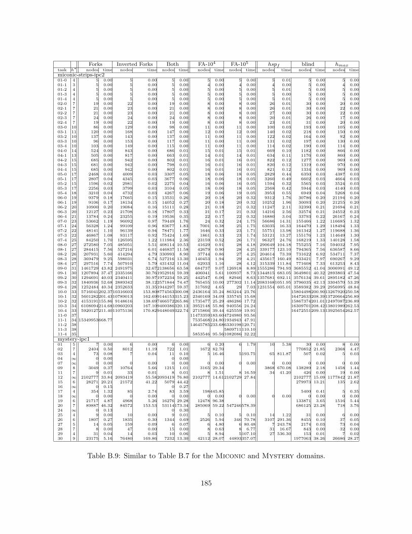
Forks Inverted Forks Both FA-104 FA-105 hspf blind hmaxtask h∗ nodes time nodes time nodes time nodes time nodes time nodes time nodes time nodes time
miconic-strips-ipc201-0 4 5 0.00 5 0.00 5 0.00 5 0.00 5 0.00 5 0.01 5 0.00 5 0.0001-1 3 5 0.00 5 0.00 5 0.00 4 0.00 4 0.00 4 0.00 5 0.00 4 0.0001-2 4 5 0.00 5 0.00 5 0.00 5 0.00 5 0.00 5 0.01 5 0.00 5 0.0001-3 4 5 0.00 5 0.00 5 0.00 5 0.00 5 0.00 5 0.00 5 0.00 5 0.0001-4 4 5 0.00 5 0.00 5 0.00 5 0.00 5 0.00 5 0.01 5 0.00 5 0.0002-0 7 19 0.00 22 0.00 19 0.00 8 0.00 8 0.00 26 0.01 30 0.00 20 0.0002-1 7 21 0.00 23 0.00 21 0.00 8 0.00 8 0.00 26 0.01 30 0.00 22 0.0002-2 7 21 0.00 23 0.00 21 0.00 8 0.00 8 0.00 27 0.00 30 0.00 22 0.0002-3 7 24 0.00 24 0.00 24 0.00 8 0.00 8 0.00 20 0.01 26 0.00 17 0.0002-4 7 19 0.00 22 0.00 19 0.00 8 0.00 8 0.00 23 0.01 31 0.00 20 0.0003-0 10 86 0.00 129 0.00 98 0.00 11 0.00 11 0.00 100 0.03 193 0.00 105 0.0003-1 11 120 0.00 168 0.00 147 0.00 12 0.00 12 0.00 140 0.02 218 0.00 150 0.0003-2 10 137 0.00 143 0.00 137 0.00 11 0.00 11 0.00 122 0.02 164 0.00 92 0.0003-3 10 96 0.00 153 0.00 117 0.00 11 0.00 11 0.00 131 0.02 197 0.00 130 0.0003-4 10 103 0.00 149 0.00 115 0.00 11 0.00 11 0.00 114 0.02 190 0.00 114 0.0004-0 14 524 0.00 843 0.00 686 0.01 15 0.01 15 0.01 669 0.10 1182 0.00 866 0.0004-1 13 505 0.00 817 0.00 663 0.01 14 0.01 14 0.01 634 0.11 1176 0.00 860 0.0004-2 15 685 0.00 942 0.00 802 0.01 16 0.01 16 0.01 822 0.12 1277 0.00 969 0.0004-3 15 681 0.00 942 0.00 798 0.01 16 0.01 16 0.01 820 0.12 1319 0.00 970 0.0004-4 15 685 0.00 942 0.00 802 0.01 16 0.01 16 0.01 821 0.12 1334 0.00 969 0.0005-0 17 2468 0.03 4009 0.03 3307 0.05 18 0.06 18 0.05 2829 0.44 6350 0.03 4387 0.0305-1 17 2807 0.04 4345 0.03 3677 0.06 18 0.06 18 0.05 3260 0.49 6602 0.03 4664 0.0305-2 15 1596 0.02 2981 0.02 2275 0.04 16 0.06 16 0.05 1594 0.32 5565 0.03 3524 0.0305-3 17 2256 0.03 3799 0.03 3104 0.05 18 0.06 18 0.05 2568 0.42 5944 0.03 4140 0.0305-4 18 3210 0.04 4732 0.03 4267 0.06 19 0.06 19 0.05 3953 0.55 6949 0.04 5268 0.0406-0 19 9379 0.18 17665 0.15 13531 0.26 20 0.18 20 0.32 9312 1.76 30786 0.20 21194 0.2006-1 19 9106 0.17 18134 0.15 14052 0.27 20 0.18 20 0.32 10252 1.96 30093 0.20 21255 0.2006-2 20 10900 0.20 19084 0.16 15111 0.28 21 0.18 21 0.32 11247 2.11 32390 0.21 21694 0.2106-3 20 12127 0.23 21708 0.18 17807 0.33 21 0.17 21 0.32 14216 2.56 32574 0.21 24552 0.2306-4 21 13784 0.24 23255 0.19 19536 0.35 22 0.17 22 0.32 16880 3.04 33793 0.22 26167 0.2407-0 23 53662 1.19 96092 0.97 79449 1.76 24 0.32 24 1.75 56686 14.31 155466 1.22 116685 1.3207-1 24 56328 1.24 99109 0.96 83677 1.83 7001 0.38 25 1.75 63035 16.33 164470 1.29 118494 1.3307-2 22 48141 1.10 96139 0.94 78471 1.77 1646 0.33 23 1.71 55751 13.98 161342 1.27 119688 1.3607-3 22 46867 1.08 93117 0.92 75424 1.69 1861 0.33 23 1.74 53121 13.27 155176 1.23 114649 1.3007-4 25 84250 1.70 126595 1.22 111984 2.36 23159 0.52 26 1.71 96327 24.76 168219 1.33 140128 1.5808-0 27 272580 7.05 485051 5.51 408114 10.53 41629 0.91 28 4.18 290649 104.18 755255 7.16 594032 7.9508-1 27 284415 7.56 527216 6.01 446837 11.58 42679 0.90 28 4.25 339177 123.10 794365 7.56 636587 8.6608-2 26 207931 5.60 414294 4.79 330993 8.90 37744 0.86 27 4.25 204614 73.39 731622 6.92 534711 7.3708-3 28 369479 9.25 598031 6.74 527216 13.30 140453 1.94 29 4.21 435617 160.49 833421 7.97 690267 9.2908-4 27 297516 7.74 507910 5.79 431432 11.04 62933 1.16 28 4.12 315339 111.84 771608 7.33 613253 8.4309-0 31 1461729 43.82 2491975 32.672138656 63.58 684737 9.07 126918 8.89 1555286 794.93 3685552 41.04 3006991 49.1209-1 30 1207894 37.47 2335166 30.761952916 59.39 406041 5.61 100937 8.73 1344815 683.05 3649801 40.32 2893803 47.5409-2 30 1294691 40.03 2340411 30.971972234 59.25 442547 6.06 82946 8.63 1357681 692.11 3576134 39.61 2895182 47.2609-3 32 1840936 52.68 2889342 38.122571844 74.47 765455 10.00 277302 11.14 20831681051.95 3796035 42.13 3304570 53.2909-4 28 1252484 40.34 2352633 31.351944297 59.37 317692 4.65 29 7.03 1231554 605.01 3589382 39.29 2956995 48.8410-0 33 5716041202.3710316603 153.808774563300.08 2436164 35.24 863244 23.76 15804498200.9013267920250.5810-1 32 5601282201.4310789013 162.699144153315.23 2340169 34.09 335745 15.68 16472633208.3913720664256.8910-2 32 4153191155.86 9148616 138.697466572265.86 1735477 25.29 486286 17.72 15867374201.0112497087236.8910-3 34 6108094214.6810960203 167.109400386320.13 3952148 55.86 940556 24.24 16309701208.4213801989262.5310-4 33 5920127211.4011075136 170.829448049322.74 2715866 39.44 625559 19.91 16472551209.1313925654262.5711-0 37 11473359183.604724980 93.5611-1 34 15349953668.77 7535468124.801934943 47.9111-2 38 14645785233.686330198120.7111-3 38 5809711110.1011-4 35 5853546 95.561082086 32.22
mystery-ipc101 5 7 0.00 6 0.00 6 0.00 6 0.20 6 1.79 10 5.38 30 0.00 8 0.0002 7 2404 0.50 8012 11.19 722 1.01 1672 82.70 770852 21.85 2368 4.4703 4 73 0.08 7 0.04 11 0.10 5 16.46 5193.75 65 811.87 507 0.02 5 0.0304 ∞ 0 0.00 0 0.0007 ∞ 0 0.00 0 0.00 0 0.00 0 0.00 0 0.00 0 0.00 0 0.00 0 0.0009 8 3049 0.37 10764 5.66 1215 1.01 3165 29.34 3868 670.08 138289 2.18 1458 1.4411 7 9 0.01 33 0.01 8 0.01 8 1.51 8 16.59 34 41.20 426 0.00 19 0.0012 ∞ 2102777 33.84 2093419 55.582093419 76.80 2102777 14.612102729 27.84 2102777 15.09 1177842 21.8715 6 28271 20.21 21572 41.22 5079 44.42 279973 13.21 135 2.6216 ∞ 0 0.15 0 0.2717 4 354 1.32 85 2.74 83 3.59 198445.85 5400 0.41 5 0.3518 ∞ 0 0.00 0 0.00 0 0.00 0 0.00 0 0.00 0 0.00 0 0.00 0 0.0019 6 21717 4.87 4968 5.26 16276 29.28 12478 96.38 133871 3.65 1516 5.4420 7 89887 46.32 84572 153.53 53114173.34 285069 59.22 547246578.39 686125 23.28 718 3.7624 ∞ 0 0.13 0 0.3025 4 9 0.00 10 0.00 9 0.01 5 0.10 5 0.10 14 1.22 31 0.00 6 0.0026 6 1807 0.27 1835 0.30 1344 0.69 2526 5.94 346 70.78 3107 291.36 8455 0.10 37 0.0527 5 14 0.05 159 0.09 6 0.07 6 4.80 6 80.48 7 243.78 2174 0.03 73 0.0428 7 8 0.00 47 0.00 15 0.00 8 0.63 8 6.77 31 16.67 843 0.00 32 0.0029 4 31 0.04 14 0.03 10 0.06 5 8.94 5107.10 27 536.30 153 0.01 7 0.0230 9 23175 5.16 76480 169.86 7232 13.30 42112 28.07 44893357.07 1977063 38.26 26686 28.27
Table B.9: Similar to Table B.7 for the Miconic and Mystery domains.
185

Forks Inverted Forks Both FA-104 FA-105 hspf blind hmaxtask h∗ nodes time nodes time nodes time nodes time nodes time nodes time nodes time nodes time
openstacks-ipc501 23 2264 0.02 3895 0.03 3070 0.05 24 0.05 24 0.06 2000 1.02 4822 0.01 4016 0.0302 23 2617 0.03 4485 0.04 3561 0.05 24 0.06 24 0.06 2378 1.07 5501 0.02 4594 0.0403 23 2264 0.02 3895 0.03 3070 0.05 24 0.06 24 0.06 2000 1.02 4822 0.01 4016 0.0304 23 2264 0.02 3895 0.03 3070 0.05 24 0.06 24 0.06 2000 1.02 4822 0.02 4016 0.0305 23 2264 0.02 3895 0.03 3070 0.05 24 0.06 24 0.05 2000 1.02 4822 0.01 4016 0.0306 45 366768 7.52 779710 18.93 587482 22.20 621008 4.85 279614 7.86 379735 217.37 882874 4.91 822514 18.7107 46 410728 8.23 760668 18.33 606782 22.53 594758 4.69 264535 7.34 405564 226.32 836647 4.62 787163 17.81
pathways-ipc501 6 1624 0.00 1299 0.00 1299 0.00 7 1.14 7 0.79 1405 0.28 1624 0.00 36 0.0002 12 2755 0.02 2307 0.01 2437 0.02 1946 2.56 13 42.11 990 0.29 2984 0.02 348 0.0103 18 44928 0.62 20416 0.25 29106 0.43 21671 6.43 14901129.23 14772 6.99 87189 1.06 4346 0.1604 17 126950 2.66 33788 0.59 58738 1.31 98484288.39 34206 27.00 456143 8.22 104068 2.61
pipesworld-notankage-ipc401 5 121 0.02 109 0.01 121 0.02 6 0.04 6 0.04 6 2.79 121 0.00 13 0.0002 12 1413 0.06 1542 0.02 1413 0.08 169 0.30 13 0.17 435 3.07 1808 0.01 792 0.0203 8 1742 0.14 3001 0.07 1742 0.18 9 1.15 9 0.69 128 3.84 3293 0.02 262 0.0204 11 7007 0.45 8911 0.22 7007 0.59 651 1.95 12 7.05 812 8.84 16088 0.11 2925 0.1305 8 4093 0.49 6805 0.26 4093 0.65 77 5.63 9 21.15 155 16.53 11128 0.12 1121 0.1506 10 12401 1.44 27377 1.34 12401 2.03 1299 5.26 61 39.31 1151 23.41 49905 0.48 7102 0.7207 8 4370 0.97 9168 0.77 4370 1.34 233 19.78 9 59.70 185 29.88 46502 0.57 2631 0.4808 10 18851 3.84 56189 6.21 20584 6.42 561 12.42 497 94.69 1673 48.84 273585 3.39 22874 3.5809 13 1092472 160.712419903 151.991092472 219.75 104875 25.48 10478 74.265513309 80.62 321861 68.9910 18 2982520 66.89 6898321439.64 111212451579.7711 20 313952 27.68 472950 29.55 313952 43.90 90598 9.20 52159 43.24 108503 625.52 710123 3.86 107061 14.5112 24 684234 75.721319980 133.58 686186 145.41 594661 12.41 416184109.43 4332961117.572467804 13.83 464982 56.8213 16 39998 6.02 117475 18.08 40226 12.69 12835 34.28 242241019.65 481045 3.14 33417 6.3814 30 13255718119.5415 26 1594863 254.432588849 192.901594863 353.40 648132 65.43 4921698 34.90 555619 105.4917 22 54373931588.68 3200672 90.0719 24 8767431150.8821 14 23833 4.02 49035 7.76 23833 7.87 3992 18.13 948159.63 157782 1.31 8966 2.4223 18 2285790 568.937047138 871.032282678 843.28 296506 49.11 104750256.13 481859 229.0024 24 7315150142.8241 12 502308 370.68 5023081092.50 114257 250.18
pipesworld-tankage-ipc401 5 77 0.02 126 0.01 105 0.02 6 3.54 6 0.13 6 3.88 128 0.00 13 0.0102 12 960 0.05 1005 0.02 960 0.06 110 3.04 13 0.20 179 6.04 1012 0.01 659 0.0203 8 20803 1.89 52139 2.46 20803 2.82 244 22.64 9 36.89 818 24.47 52983 0.77 1802 1.3304 11 110284 8.06 157722 9.60 110284 14.05 3892 16.68 12155.03 8116 64.68 221429 3.06 41540 14.4905 8 6531 0.86 13148 1.03 6531 1.32 376 15.46 9120.06 313 59.99 12764 0.21 2834 1.6106 10 20171 2.41 43583 4.32 20171 4.41 1794328.18 11201.44 3102 97.31 58487 0.87 15746 6.6107 8 202706 73.832643752 1379.11 202706 208.81 2695 339.765404036198.08 104531 420.4708 11 96043191.7711 22 2345399 296.872629204 662.942365735 838.85 660104 28.60 660102162.93 4116344 30.67 752867 334.4213 16 188517122.1115 30 96520911721.67 2546587141.1217 44 12850247352.4621 14 839847 250.39 13241 69.80 4423951 65.44 126845 222.2331 39 1501847 240.381568963 661.881504072 850.16 1357801124.64 1726598 13.56 919764 381.66
rovers-ipc501 10 147 0.00 147 0.00 147 0.00 11 0.03 11 0.03 48 0.07 1104 0.00 283 0.0002 8 44 0.00 44 0.00 44 0.00 9 0.00 9 0.00 16 0.03 254 0.00 129 0.0003 11 672 0.01 419 0.00 448 0.01 12 0.11 12 0.12 804 0.16 3543 0.02 757 0.0004 8 47 0.00 20 0.00 24 0.00 9 0.04 9 0.04 58 0.08 897 0.00 223 0.0005 22 808084 22.61 410712 9.23 522937 18.29 617267 11.48 375808 18.46 298400 101.658559690126.19 4318309 81.5307 18 4546797 191.34 741649 21.011682245 102.77 3280884 51.022212903 59.20 1459792 866.93 9618062 199.9112 19 1529551 76.46 5187273166.77
satellite-ipc401 9 24 0.00 32 0.00 29 0.00 10 0.00 10 0.00 46 0.06 89 0.00 59 0.0002 13 86 0.00 337 0.00 241 0.01 14 0.01 14 0.01 646 0.21 1728 0.01 940 0.0003 11 2249 0.08 656 0.01 728 0.04 12 0.56 12 0.64 1945 0.93 15185 0.17 6822 0.1104 17 9817 0.57 14860 0.38 11250 0.76 4152 0.99 18 4.43 15890 9.50 345663 4.70 180815 3.3705 15 279569 49.47 46453 4.92 61692 18.85 81972 7.26 148667 69.28 267513 565.1806 20 1496577 92.221572327 51.681518261 105.65 2769229 74.73 307962 32.52 10751017 371.43
Table B.10: Similar to Table B.7 for the Openstacks, Pathways, Pipesworld-NoTankage,Pipesworld-Tankage, Rovers, and Satellite domains.
186
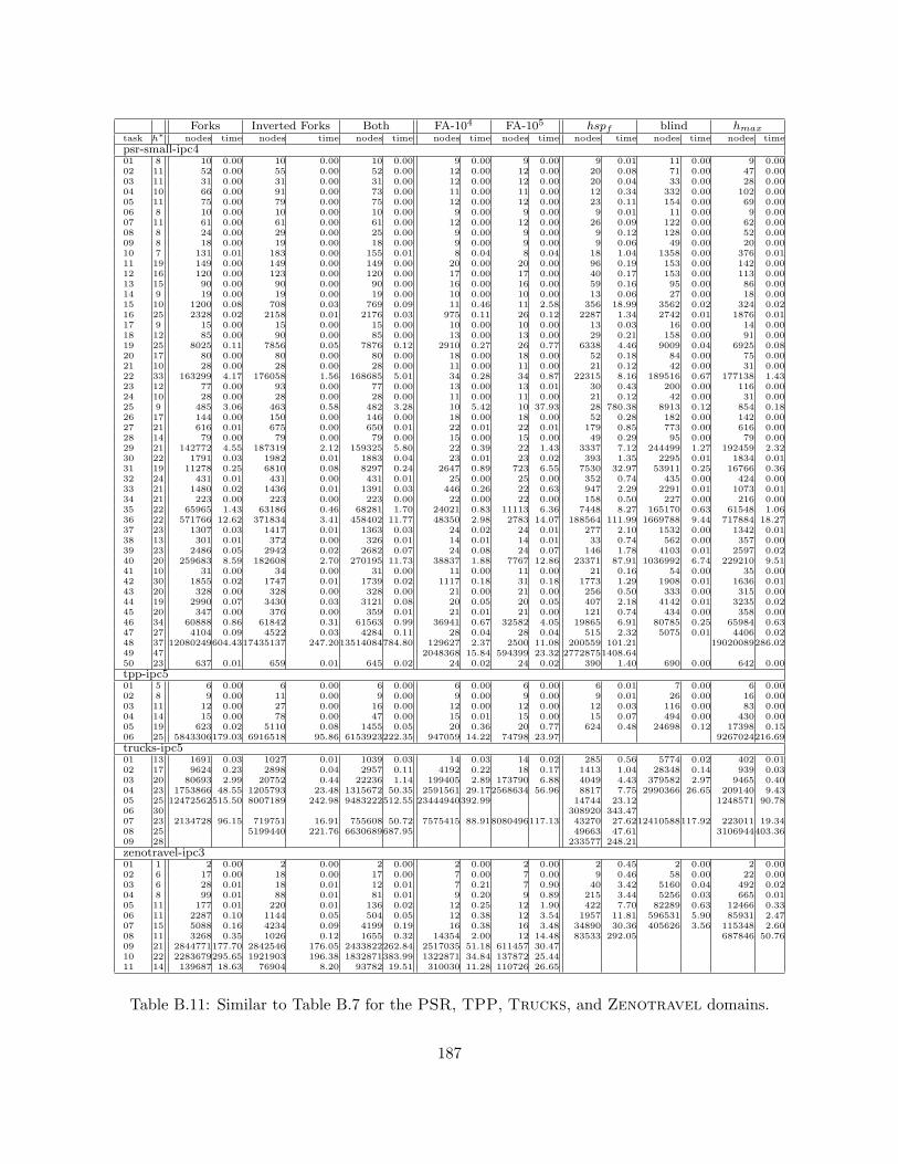
Forks Inverted Forks Both FA-104 FA-105 hspf blind hmaxtask h∗ nodes time nodes time nodes time nodes time nodes time nodes time nodes time nodes time
psr-small-ipc401 8 10 0.00 10 0.00 10 0.00 9 0.00 9 0.00 9 0.01 11 0.00 9 0.0002 11 52 0.00 55 0.00 52 0.00 12 0.00 12 0.00 20 0.08 71 0.00 47 0.0003 11 31 0.00 31 0.00 31 0.00 12 0.00 12 0.00 20 0.04 33 0.00 28 0.0004 10 66 0.00 91 0.00 73 0.00 11 0.00 11 0.00 12 0.34 332 0.00 102 0.0005 11 75 0.00 79 0.00 75 0.00 12 0.00 12 0.00 23 0.11 154 0.00 69 0.0006 8 10 0.00 10 0.00 10 0.00 9 0.00 9 0.00 9 0.01 11 0.00 9 0.0007 11 61 0.00 61 0.00 61 0.00 12 0.00 12 0.00 26 0.09 122 0.00 62 0.0008 8 24 0.00 29 0.00 25 0.00 9 0.00 9 0.00 9 0.12 128 0.00 52 0.0009 8 18 0.00 19 0.00 18 0.00 9 0.00 9 0.00 9 0.06 49 0.00 20 0.0010 7 131 0.01 183 0.00 155 0.01 8 0.04 8 0.04 18 1.04 1358 0.00 376 0.0111 19 149 0.00 149 0.00 149 0.00 20 0.00 20 0.00 96 0.19 153 0.00 142 0.0012 16 120 0.00 123 0.00 120 0.00 17 0.00 17 0.00 40 0.17 153 0.00 113 0.0013 15 90 0.00 90 0.00 90 0.00 16 0.00 16 0.00 59 0.16 95 0.00 86 0.0014 9 19 0.00 19 0.00 19 0.00 10 0.00 10 0.00 13 0.06 27 0.00 18 0.0015 10 1200 0.08 708 0.03 769 0.09 11 0.46 11 2.58 356 18.99 3562 0.02 324 0.0216 25 2328 0.02 2158 0.01 2176 0.03 975 0.11 26 0.12 2287 1.34 2742 0.01 1876 0.0117 9 15 0.00 15 0.00 15 0.00 10 0.00 10 0.00 13 0.03 16 0.00 14 0.0018 12 85 0.00 90 0.00 85 0.00 13 0.00 13 0.00 29 0.21 158 0.00 91 0.0019 25 8025 0.11 7856 0.05 7876 0.12 2910 0.27 26 0.77 6338 4.46 9009 0.04 6925 0.0820 17 80 0.00 80 0.00 80 0.00 18 0.00 18 0.00 52 0.18 84 0.00 75 0.0021 10 28 0.00 28 0.00 28 0.00 11 0.00 11 0.00 21 0.12 42 0.00 31 0.0022 33 163299 4.17 176058 1.56 168685 5.01 34 0.28 34 0.87 22315 8.16 189516 0.67 177138 1.4323 12 77 0.00 93 0.00 77 0.00 13 0.00 13 0.01 30 0.43 200 0.00 116 0.0024 10 28 0.00 28 0.00 28 0.00 11 0.00 11 0.00 21 0.12 42 0.00 31 0.0025 9 485 3.06 463 0.58 482 3.28 10 5.42 10 37.93 28 780.38 8913 0.12 854 0.1826 17 144 0.00 150 0.00 146 0.00 18 0.00 18 0.00 52 0.28 182 0.00 142 0.0027 21 616 0.01 675 0.00 650 0.01 22 0.01 22 0.01 179 0.85 773 0.00 616 0.0028 14 79 0.00 79 0.00 79 0.00 15 0.00 15 0.00 49 0.29 95 0.00 79 0.0029 21 142772 4.55 187319 2.12 159325 5.80 22 0.39 22 1.43 3337 7.12 244499 1.27 192459 2.3230 22 1791 0.03 1982 0.01 1883 0.04 23 0.01 23 0.02 393 1.35 2295 0.01 1834 0.0131 19 11278 0.25 6810 0.08 8297 0.24 2647 0.89 723 6.55 7530 32.97 53911 0.25 16766 0.3632 24 431 0.01 431 0.00 431 0.01 25 0.00 25 0.00 352 0.74 435 0.00 424 0.0033 21 1480 0.02 1436 0.01 1391 0.03 446 0.26 22 0.63 947 2.29 2291 0.01 1073 0.0134 21 223 0.00 223 0.00 223 0.00 22 0.00 22 0.00 158 0.50 227 0.00 216 0.0035 22 65965 1.43 63186 0.46 68281 1.70 24021 0.83 11113 6.36 7448 8.27 165170 0.63 61548 1.0636 22 571766 12.62 371834 3.41 458402 11.77 48350 2.98 2783 14.07 188564 111.99 1669788 9.44 717884 18.2737 23 1307 0.03 1417 0.01 1363 0.03 24 0.02 24 0.01 277 2.10 1532 0.00 1342 0.0138 13 301 0.01 372 0.00 326 0.01 14 0.01 14 0.01 33 0.74 562 0.00 357 0.0039 23 2486 0.05 2942 0.02 2682 0.07 24 0.08 24 0.07 146 1.78 4103 0.01 2597 0.0240 20 259683 8.59 182608 2.70 270195 11.73 38837 1.88 7767 12.86 23371 87.91 1036992 6.74 229210 9.5141 10 31 0.00 34 0.00 31 0.00 11 0.00 11 0.00 21 0.16 54 0.00 35 0.0042 30 1855 0.02 1747 0.01 1739 0.02 1117 0.18 31 0.18 1773 1.29 1908 0.01 1636 0.0143 20 328 0.00 328 0.00 328 0.00 21 0.00 21 0.00 256 0.50 333 0.00 315 0.0044 19 2990 0.07 3430 0.03 3121 0.08 20 0.05 20 0.05 407 2.18 4142 0.01 3235 0.0245 20 347 0.00 376 0.00 359 0.01 21 0.01 21 0.00 121 0.74 434 0.00 358 0.0046 34 60888 0.86 61842 0.31 61563 0.99 36941 0.67 32582 4.05 19865 6.91 80785 0.25 65984 0.6347 27 4104 0.09 4522 0.03 4284 0.11 28 0.04 28 0.04 515 2.32 5075 0.01 4406 0.0248 37 12080249604.4317435137 247.2013514084784.80 129627 2.37 2500 11.08 200559 101.21 19020089286.0249 47 2048368 15.84 594399 23.32 27728751408.6450 23 637 0.01 659 0.01 645 0.02 24 0.02 24 0.02 390 1.40 690 0.00 642 0.00
tpp-ipc501 5 6 0.00 6 0.00 6 0.00 6 0.00 6 0.00 6 0.01 7 0.00 6 0.0002 8 9 0.00 11 0.00 9 0.00 9 0.00 9 0.00 9 0.01 26 0.00 16 0.0003 11 12 0.00 27 0.00 16 0.00 12 0.00 12 0.00 12 0.03 116 0.00 83 0.0004 14 15 0.00 78 0.00 47 0.00 15 0.01 15 0.00 15 0.07 494 0.00 430 0.0005 19 623 0.02 5110 0.08 1455 0.05 20 0.36 20 0.77 624 0.48 24698 0.12 17398 0.1506 25 5843306179.03 6916518 95.86 6153923222.35 947059 14.22 74798 23.97 9267024216.69
trucks-ipc501 13 1691 0.03 1027 0.01 1039 0.03 14 0.03 14 0.02 285 0.56 5774 0.02 402 0.0102 17 9624 0.23 2898 0.04 2957 0.11 4192 0.22 18 0.17 1413 1.04 28348 0.14 939 0.0303 20 80693 2.99 20752 0.44 22236 1.14 199405 2.89 173790 6.88 4049 4.43 379582 2.97 9465 0.4004 23 1753866 48.55 1205793 23.48 1315672 50.35 2591561 29.172568634 56.96 8817 7.75 2990366 26.65 209140 9.4305 25 12472562515.50 8007189 242.98 9483222512.55 23444940392.99 14744 23.12 1248571 90.7806 30 308920 343.4707 23 2134728 96.15 719751 16.91 755608 50.72 7575415 88.918080496117.13 43270 27.6212410588117.92 223011 19.3408 25 5199440 221.76 6630689687.95 49663 47.61 3106944403.3609 28 233577 248.21
zenotravel-ipc301 1 2 0.00 2 0.00 2 0.00 2 0.00 2 0.00 2 0.45 2 0.00 2 0.0002 6 17 0.00 18 0.00 17 0.00 7 0.00 7 0.00 9 0.46 58 0.00 22 0.0003 6 28 0.01 18 0.01 12 0.01 7 0.21 7 0.90 40 3.42 5160 0.04 492 0.0204 8 99 0.01 88 0.01 81 0.01 9 0.20 9 0.89 215 3.44 5256 0.03 665 0.0105 11 177 0.01 220 0.01 136 0.02 12 0.25 12 1.90 422 7.70 82289 0.63 12466 0.3306 11 2287 0.10 1144 0.05 504 0.05 12 0.38 12 3.54 1957 11.81 596531 5.90 85931 2.4707 15 5088 0.16 4234 0.09 4199 0.19 16 0.38 16 3.48 34890 30.36 405626 3.56 115348 2.6008 11 3268 0.35 1026 0.12 1655 0.32 14354 2.00 12 14.48 83533 292.05 687846 50.7609 21 2844771177.70 2842546 176.05 2433822262.84 2517035 51.18 611457 30.4710 22 2283679295.65 1921903 196.38 1832871383.99 1322871 34.84 137872 25.4411 14 139687 18.63 76904 8.20 93782 19.51 310030 11.28 110726 26.65
Table B.11: Similar to Table B.7 for the PSR, TPP, Trucks, and Zenotravel domains.
187
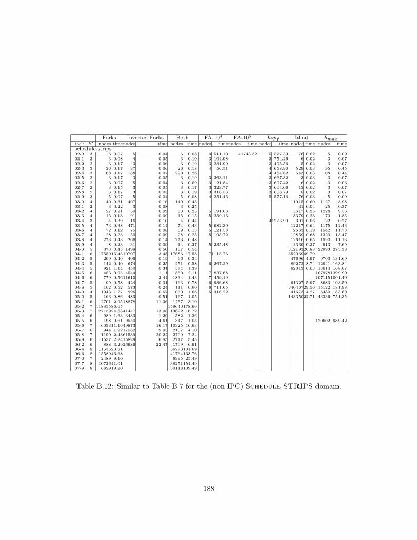
Forks Inverted Forks Both FA-104 FA-105 hspf blind hmaxtask h∗ nodes timenodes time nodes time nodes timenodes time nodes time nodes time nodes time
schedule-strips02-0 3 5 0.07 5 0.04 5 0.08 4 511.10 41743.32 5 577.39 76 0.02 5 0.0902-1 2 3 0.08 4 0.05 3 0.10 3 104.98 3 754.26 6 0.02 3 0.0702-2 2 3 0.17 3 0.06 3 0.19 3 231.99 3 495.56 5 0.02 3 0.0702-3 3 26 0.17 37 0.06 26 0.18 4 56.51 4 658.90 529 0.03 95 0.4502-4 3 68 0.17 188 0.07 220 0.26 4 484.62 543 0.03 108 0.4402-5 2 3 0.17 3 0.05 3 0.19 3 363.11 3 667.32 3 0.03 3 0.0702-6 2 3 0.07 5 0.04 3 0.09 3 121.84 3 697.42 6 0.02 3 0.0602-7 2 3 0.15 3 0.05 3 0.17 3 323.77 3 604.06 13 0.02 3 0.0702-8 2 3 0.17 3 0.05 3 0.19 3 316.53 3 668.79 8 0.02 3 0.0702-9 3 5 0.07 5 0.04 5 0.08 4 251.46 5 577.16 76 0.03 5 0.0903-0 4 40 0.31 407 0.16 140 0.45 11915 0.60 1127 8.9803-1 2 3 0.22 3 0.08 3 0.25 31 0.04 25 0.3703-2 4 27 0.21 50 0.09 33 0.25 5 191.03 3617 0.23 1228 9.5603-3 4 15 0.13 91 0.09 15 0.15 5 259.13 3379 0.23 170 1.8503-4 3 4 0.39 16 0.10 4 0.44 41223.90 301 0.06 22 0.2703-5 4 73 0.38 471 0.14 74 0.43 5 682.30 12217 0.64 1175 12.4303-6 4 72 0.12 75 0.08 69 0.13 5 121.58 2663 0.19 1542 11.7303-7 4 28 0.23 50 0.09 28 0.25 5 195.72 12859 0.68 1323 13.4703-8 4 273 0.43 266 0.14 273 0.48 12616 0.65 1590 11.1303-9 4 8 0.23 31 0.09 14 0.27 5 235.48 4339 0.27 913 7.6904-0 5 373 0.45 1498 0.50 167 0.54 31219326.88 22993 273.3804-1 6 1755915.4510707 3.48 17686 17.58 71115.76 55206949.7904-2 5 209 0.40 406 0.19 66 0.34 47696 4.97 9703 131.6904-3 5 142 0.40 674 0.25 251 0.58 6 267.29 89272 8.74 12941 163.8404-4 5 921 1.14 450 0.31 574 1.39 62013 6.03 13614 168.0704-5 6 483 0.95 4544 1.11 850 2.11 7 837.68 1079781399.9904-6 6 779 0.5611610 2.44 1834 1.43 7 459.19 1071151001.4004-7 5 99 0.58 424 0.31 163 0.78 6 936.68 61327 5.97 8683 103.5004-8 5 102 0.52 573 0.24 111 0.60 6 711.65 34046729.56 15122 181.9804-9 4 1043 1.27 996 0.67 1050 1.66 5 316.22 41673 4.27 5480 83.6905-0 5 163 0.86 483 0.51 167 1.05 14335022.71 43336 751.3505-1 6 2701 2.9518878 11.36 1257 3.1005-2 7 11885586.65 158640178.6605-3 7 2715924.8841447 13.08 13622 16.7205-4 6 989 1.63 3433 1.29 582 1.3605-5 6 198 0.61 9550 4.61 347 1.05 120602 989.4205-6 7 603311.1649873 16.17 10325 16.6305-7 6 944 1.9217562 9.03 2107 4.1005-8 7 1190 2.4361539 20.22 2709 7.2405-9 6 1537 2.2415829 6.85 2717 5.4506-2 6 888 3.2926986 22.47 1709 6.9106-4 8 1153520.81 56273131.6906-6 8 1558946.68 41764133.7607-0 7 2489 9.10 6995 25.4907-7 8 1072641.01 38251154.4907-9 8 682919.20 30148109.49
Table B.12: Similar to Table B.7 for the (non-IPC) Schedule-STRIPS domain.
188
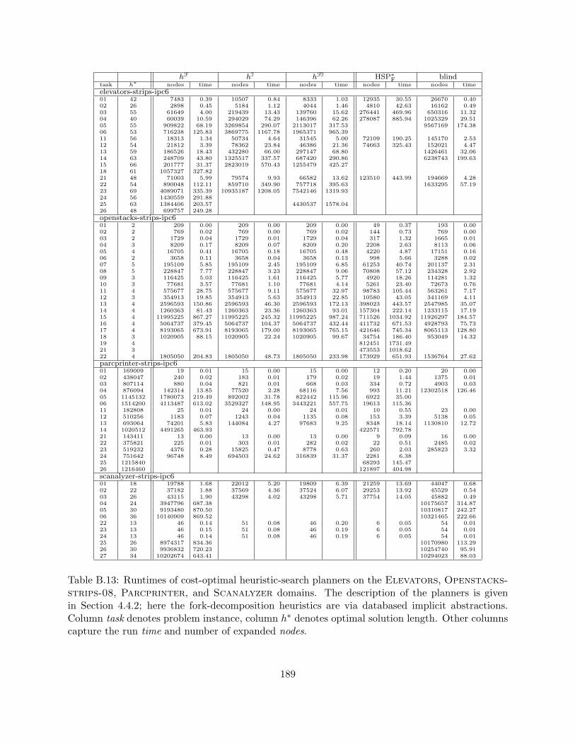
hF hI hFI HSP∗F blindtask h∗ nodes time nodes time nodes time nodes time nodes time
elevators-strips-ipc601 42 7483 0.39 10507 0.84 8333 1.03 12935 30.55 26670 0.4002 26 2898 0.45 5184 1.12 4044 1.46 4810 42.63 16162 0.4903 55 61649 4.00 219439 13.43 139760 15.62 276441 469.96 650316 11.3204 40 60039 10.59 294029 74.29 146396 62.26 278087 885.94 1025329 29.5105 55 909822 68.19 3269854 290.07 2113017 317.53 9567169 174.3806 53 716238 125.83 3869775 1167.78 1965371 965.3911 56 18313 1.34 50734 4.64 31545 5.00 72109 190.25 145170 2.5312 54 21812 3.39 78362 23.84 46386 21.36 74663 325.43 152021 4.4713 59 186526 18.43 432280 66.00 297147 68.80 1426461 32.0614 63 248709 43.80 1325517 337.57 687420 290.86 6238743 199.6315 66 201777 31.37 2823019 570.43 1255479 425.2718 61 1057327 327.8221 48 71003 5.99 79574 9.93 66582 13.62 123510 443.99 194669 4.2822 54 890048 112.11 859710 349.90 757718 395.63 1633295 57.1923 69 4089071 335.39 10935187 1208.05 7542146 1319.9324 56 1430559 291.8825 63 1384406 203.57 4430537 1578.0426 48 699757 249.28
openstacks-strips-ipc601 2 209 0.00 209 0.00 209 0.00 49 0.37 193 0.0002 2 769 0.02 769 0.00 769 0.02 144 0.73 769 0.0003 2 1729 0.04 1729 0.01 1729 0.04 317 1.32 1665 0.0104 3 8209 0.17 8209 0.07 8209 0.20 2208 2.63 8113 0.0605 4 16705 0.41 16705 0.18 16705 0.48 4220 4.87 17151 0.1606 2 3658 0.11 3658 0.04 3658 0.13 998 5.66 3288 0.0207 5 195109 5.85 195109 2.45 195109 6.85 61253 40.74 201137 2.3108 5 228847 7.77 228847 3.23 228847 9.06 70808 57.12 234328 2.9209 3 116425 5.03 116425 1.61 116425 5.77 4920 18.26 114281 1.3210 3 77681 3.57 77681 1.10 77681 4.14 5261 23.40 72673 0.7611 4 575677 28.75 575677 9.11 575677 32.97 98783 105.44 563261 7.1712 3 354913 19.85 354913 5.63 354913 22.85 10580 43.05 341169 4.1113 4 2596593 150.86 2596593 46.30 2596593 172.13 398023 443.57 2547985 35.0714 4 1260363 81.43 1260363 23.36 1260363 93.01 157304 222.14 1233115 17.1915 4 11995225 867.27 11995225 245.32 11995225 987.24 711526 1034.92 11926297 184.5716 4 5064737 379.45 5064737 104.37 5064737 432.44 411732 671.53 4928793 75.7317 4 8193065 673.91 8193065 179.00 8193065 765.15 421646 745.34 8065113 128.8018 3 1020905 88.15 1020905 22.24 1020905 99.67 34754 186.40 953049 14.3219 4 812451 1731.4921 3 473553 1018.6222 4 1805050 204.83 1805050 48.73 1805050 233.98 173929 651.93 1536764 27.62
parcprinter-strips-ipc601 169009 19 0.01 15 0.00 15 0.00 12 0.20 20 0.0002 438047 240 0.02 183 0.01 179 0.02 19 1.44 1375 0.0103 807114 880 0.04 821 0.01 668 0.03 334 0.72 4903 0.0304 876094 142314 13.85 77520 2.28 68116 7.56 993 11.21 12302518 126.4605 1145132 1780073 219.49 892002 31.78 822442 115.96 6922 35.0006 1514200 4113487 613.02 3529327 148.95 3443221 557.75 19613 115.3611 182808 25 0.01 24 0.00 24 0.01 10 0.55 23 0.0012 510256 1183 0.07 1243 0.04 1135 0.08 153 3.39 5138 0.0513 693064 74201 5.83 144084 4.27 97683 9.25 8348 18.14 1130810 12.7214 1020512 4491265 463.93 422571 792.7821 143411 13 0.00 13 0.00 13 0.00 9 0.09 16 0.0022 375821 225 0.01 303 0.01 282 0.02 22 0.51 2485 0.0223 519232 4376 0.28 15825 0.47 8778 0.63 260 2.03 285823 3.3224 751642 96748 8.49 694503 24.62 316839 31.37 2281 6.3825 1215840 68293 145.4726 1216460 121897 404.98
scanalyzer-strips-ipc601 18 19788 1.68 22012 5.20 19809 6.39 21259 13.69 44047 0.6802 22 37182 1.88 37569 4.36 37524 6.07 29253 13.92 45529 0.5403 26 43115 1.90 43298 4.02 43298 5.71 37754 14.05 45882 0.4904 24 3947796 687.38 10175657 314.8705 30 9193480 870.50 10310817 242.2706 36 10140909 869.52 10321465 222.6622 13 46 0.14 51 0.08 46 0.20 6 0.05 54 0.0123 13 46 0.15 51 0.08 46 0.19 6 0.05 54 0.0124 13 46 0.14 51 0.08 46 0.19 6 0.05 54 0.0125 26 8974317 834.36 10170980 113.2926 30 9936832 720.23 10254740 95.9127 34 10202674 643.41 10294023 88.03
Table B.13: Runtimes of cost-optimal heuristic-search planners on the Elevators, Openstacks-strips-08, Parcprinter, and Scanalyzer domains. The description of the planners is givenin Section 4.4.2; here the fork-decomposition heuristics are via databased implicit abstractions.Column task denotes problem instance, column h∗ denotes optimal solution length. Other columnscapture the run time and number of expanded nodes.
189
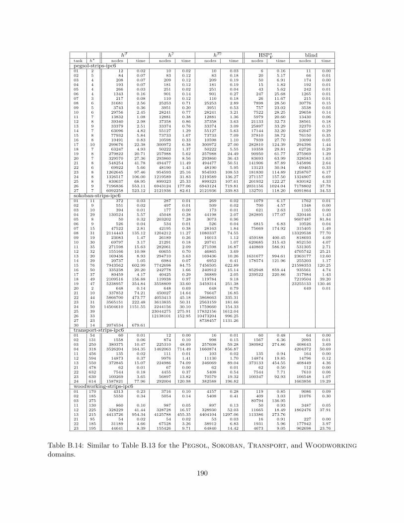
hF hI hFI HSP∗F blindtask h∗ nodes time nodes time nodes time nodes time nodes time
pegsol-strips-ipc601 2 12 0.02 10 0.02 10 0.03 6 0.16 11 0.0002 5 84 0.07 83 0.12 83 0.18 20 5.17 66 0.0103 4 208 0.07 209 0.12 209 0.19 50 6.91 174 0.0004 4 193 0.07 181 0.12 181 0.19 15 1.82 192 0.0105 4 266 0.03 251 0.02 251 0.04 43 5.62 242 0.0106 4 1343 0.16 901 0.14 901 0.27 247 25.68 1265 0.0107 3 217 0.08 110 0.12 110 0.18 26 11.67 215 0.0108 6 31681 2.56 25253 0.71 25253 2.89 7898 28.50 30776 0.1509 5 3743 0.36 3951 0.20 3951 0.53 757 23.02 3538 0.0310 6 29756 2.45 28241 0.77 28241 3.21 7522 28.25 29658 0.1411 7 13832 1.08 12881 0.38 12881 1.36 5979 20.60 13430 0.0612 8 39340 2.98 37358 0.86 37358 3.63 21133 32.73 38561 0.1813 9 33379 2.51 33374 0.76 33374 3.09 25897 33.29 32370 0.1514 7 63096 4.82 55127 1.29 55127 5.63 17144 32.20 62047 0.2915 8 77932 5.84 73733 1.67 73733 7.09 37810 38.72 76150 0.3516 8 10491 0.83 10598 0.33 10598 1.10 7939 27.70 10090 0.0517 10 299676 22.38 300972 6.38 300972 27.00 282810 124.39 294396 1.4418 7 63247 4.93 50222 1.37 50222 5.55 10358 29.81 62726 0.2919 8 279822 20.71 257988 5.62 257988 24.49 90950 61.77 275969 1.2920 7 329570 27.36 293860 8.56 293860 36.43 83693 63.99 328583 1.6321 8 548254 41.78 494477 11.49 494477 50.51 141906 87.89 545896 2.6422 6 69922 5.66 48190 1.43 48190 5.95 13123 30.94 69465 0.3323 8 1262645 97.46 954593 25.16 954593 108.53 181830 114.89 1258767 6.1724 8 1326517 106.00 1219589 31.83 1219589 136.27 271157 157.50 1324907 6.6925 8 830637 68.95 899323 25.33 899323 107.61 201932 122.27 830182 4.3326 9 7196836 553.11 6943124 177.06 6943124 719.81 2031156 1024.04 7178802 37.7827 7 6092258 523.12 2121936 82.61 2121936 339.83 132701 118.20 6091864 34.53
sokoban-strips-ipc601 11 372 0.03 287 0.01 269 0.02 1079 6.17 1762 0.0102 9 551 0.02 497 0.01 509 0.02 700 4.57 1348 0.0003 10 394 0.01 177 0.00 173 0.01 621 2.63 1165 0.0004 29 130524 5.57 45048 0.28 44198 2.07 282895 177.07 320446 1.4305 8 50 0.32 203202 7.28 3073 0.96 9607487 81.8406 9 526 0.04 534 0.01 526 0.04 6815 6.83 10526 0.0407 15 47522 2.81 42195 0.38 28163 1.84 75669 174.92 315405 1.4908 31 2114443 135.12 1204212 11.27 1080337 74.55 13329538 77.7009 19 23083 1.47 26189 0.26 16013 1.12 459188 400.45 818693 4.0910 30 69797 3.17 21291 0.18 20741 1.07 620685 315.43 852150 4.0711 35 271598 15.63 282061 2.09 271598 16.87 440869 586.91 531305 2.7112 32 155166 10.98 60655 0.70 46865 3.69 4705742 25.2113 20 169436 8.93 294710 3.63 169436 10.26 1631677 994.61 2363177 12.6014 29 20737 1.05 6984 0.07 6952 0.41 178574 121.96 255203 1.1715 76 7943562 602.99 7742698 84.75 7456505 622.89 21598353 120.2516 50 335238 20.20 242778 1.66 240912 15.14 852948 859.44 935561 4.7417 37 80459 4.17 40425 0.29 36889 2.05 239522 220.86 317984 1.4318 49 2109516 156.88 119938 0.97 119784 9.18 7219504 39.2019 47 5238957 354.84 3558809 33.60 3459314 251.38 23255133 130.4620 2 648 0.14 648 0.69 648 0.79 649 0.0121 10 337852 74.21 450027 14.64 76647 16.8522 44 5866700 473.77 4053413 45.18 3868663 335.3123 31 3565151 222.48 3613835 50.31 2563159 181.6624 50 14504610 1151.55 2244156 30.10 1759660 154.3325 39 23044275 275.91 17832156 1612.0426 33 12138101 152.95 10473204 996.2527 23 8738457 1131.2630 14 2074534 679.61
transport-strips-ipc601 54 60 0.01 12 0.00 16 0.01 60 0.48 64 0.0002 131 1558 0.06 874 0.10 998 0.15 1567 6.36 2093 0.0103 250 380375 10.47 225310 48.69 257608 59.28 380982 274.86 408643 3.6904 318 3526204 164.35 1462063 714.49 1660874 856.87 4204372 50.6911 456 135 0.02 111 0.01 103 0.02 135 0.94 164 0.0012 594 14873 0.37 9976 1.41 11130 1.70 14874 19.85 14796 0.1213 550 372845 15.07 224986 74.09 246069 89.04 373133 454.55 408449 4.3621 478 62 0.01 67 0.00 62 0.01 62 0.50 112 0.0022 632 7544 0.18 4455 0.37 5408 0.54 7544 7.71 7610 0.0623 630 100269 3.65 56897 13.82 70579 19.32 100347 92.93 106548 1.0724 614 1587821 77.96 292004 120.98 382588 196.82 1663856 19.29
woodworking-strips-ipc601 170 4313 0.23 3716 0.10 4157 0.28 119 0.85 9086 0.0902 185 5550 0.34 5054 0.14 5408 0.41 409 3.03 21076 0.3003 275 80794 136.9511 130 860 0.10 987 0.05 897 0.13 50 0.93 3487 0.0512 225 328229 41.44 328728 16.57 328930 52.03 11665 18.49 1862476 37.9113 215 4413726 954.34 4125788 455.35 4404104 1297.06 113386 273.7621 95 54 0.02 54 0.02 53 0.03 16 0.91 227 0.0022 185 31189 4.66 67528 3.26 38912 6.83 1931 5.96 177942 3.9723 195 44641 8.39 155426 9.71 64840 14.42 4673 9.05 962698 23.76
Table B.14: Similar to Table B.13 for the Pegsol, Sokoban, Transport, and Woodworkingdomains.
190
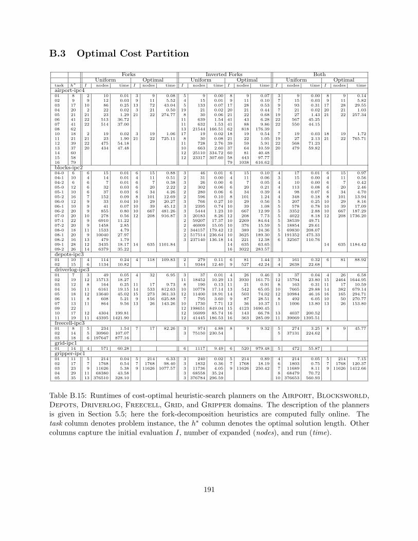
B.3 Optimal Cost Partition
Forks Inverted Forks BothUniform Optimal Uniform Optimal Uniform Optimal
task h∗ I nodes time I nodes time I nodes time I nodes time I nodes time I nodes time
airport-ipc401 8 2 10 0.01 3 9 0.08 5 9 0.00 8 9 0.07 3 9 0.00 8 9 0.1402 9 9 12 0.03 9 11 5.52 4 15 0.01 9 11 0.10 7 15 0.03 9 11 5.8203 17 10 86 0.25 13 72 43.04 5 133 0.07 17 28 0.53 9 93 0.31 17 28 29.5504 20 2 22 0.02 3 21 0.50 19 21 0.02 20 21 0.44 7 21 0.02 20 21 1.0305 21 21 23 1.29 21 22 274.77 8 30 0.06 21 22 0.68 19 27 1.43 21 22 257.3406 41 22 513 36.72 11 639 1.54 41 43 6.28 22 567 45.2507 41 22 514 37.00 11 632 1.53 41 88 9.86 22 550 44.1508 62 13 21544 166.51 62 818 176.3910 18 2 19 0.02 3 19 1.06 17 19 0.02 18 19 0.54 7 19 0.03 18 19 1.7211 21 21 23 1.90 21 22 725.11 8 30 0.08 21 22 1.05 19 27 2.13 21 22 765.7112 39 22 475 54.18 11 728 2.76 39 59 5.91 22 568 71.2313 37 20 434 47.48 10 663 2.60 37 64 10.59 20 479 59.8214 60 12 25110 334.72 60 81 40.4815 58 12 23317 307.60 58 443 97.7716 79 79 1038 616.62
blocks-ipc204-0 6 6 15 0.01 6 15 0.88 3 46 0.01 6 15 0.10 4 17 0.01 6 15 0.9704-1 10 4 14 0.01 4 11 0.51 2 31 0.00 4 11 0.06 3 15 0.00 4 11 0.5604-2 6 6 7 0.01 6 7 0.38 3 26 0.00 6 7 0.05 4 10 0.00 6 7 0.4205-0 12 6 32 0.03 6 20 2.22 2 302 0.06 6 20 0.21 4 113 0.08 6 20 2.4605-1 10 6 37 0.03 6 34 4.26 2 280 0.06 6 34 0.39 4 98 0.07 6 34 4.7005-2 16 7 152 0.09 8 101 12.69 2 596 0.10 8 101 1.24 4 348 0.18 8 101 13.9406-0 12 9 33 0.04 10 29 20.27 3 766 0.27 10 29 0.56 5 207 0.25 10 29 8.1606-1 10 9 41 0.07 10 39 45.12 3 2395 0.74 10 39 1.08 5 578 0.78 10 39 17.0906-2 20 9 855 0.80 10 667 481.26 3 5444 1.23 10 667 12.99 5 3352 2.88 10 667 187.2907-0 20 10 278 0.56 12 208 916.87 3 20183 8.26 12 208 7.73 5 4022 8.18 12 208 1736.2007-1 22 9 6910 11.22 2 59207 17.37 10 2269 84.64 5 38539 49.7107-2 20 9 1458 2.85 2 46009 15.05 10 376 15.59 5 18854 29.6108-0 18 11 1533 4.79 2 344157 179.42 12 389 24.36 5 69830 208.0708-1 20 9 10040 27.97 2 517514 236.64 10 3625 189.30 5 191352 475.3308-2 16 13 479 1.79 3 237140 136.18 14 221 12.38 6 32567 110.7609-1 28 12 3435 18.17 14 635 1101.84 14 635 63.65 14 635 1184.4209-2 26 14 6379 35.22 16 3022 283.57
depots-ipc301 10 4 114 0.24 4 118 109.83 2 279 0.11 6 81 1.44 3 161 0.32 6 81 88.9202 15 6 1134 10.82 1 9344 12.40 9 527 42.24 4 2638 22.68
driverlog-ipc301 7 3 49 0.05 4 32 6.95 3 37 0.01 4 26 0.46 3 37 0.04 4 26 6.5802 19 12 15713 18.27 11 18452 10.29 13 3930 161.75 12 15794 23.80 15 2464 1644.9503 12 8 164 0.25 11 17 9.73 8 190 0.13 11 21 0.91 8 163 0.31 11 17 10.5904 16 11 6161 19.15 14 533 812.63 10 10778 17.14 13 542 65.05 10 7665 29.88 14 382 679.1405 18 12 13640 45.02 15 273 361.33 12 11400 18.91 14 503 74.02 12 10984 46.16 16 165 294.7106 11 8 608 5.21 9 156 625.88 7 795 3.60 9 87 28.51 8 492 6.05 10 50 270.7707 13 11 864 9.56 13 26 143.26 10 1730 7.71 12 36 10.37 11 1006 13.80 13 26 153.8009 22 12 198651 849.04 15 4123 1690.4510 17 12 4304 199.81 12 16099 85.74 16 143 66.78 13 4037 200.5211 19 11 43395 1421.90 12 41445 186.53 16 363 285.09 11 39069 1395.51
freecell-ipc301 8 5 234 1.54 7 17 82.26 3 974 4.88 8 9 9.32 5 274 3.25 8 9 45.7702 14 5 30960 107.07 3 75150 230.54 5 37131 224.6203 18 6 197647 877.16
grid-ipc101 14 4 571 60.28 6 1117 9.49 6 520 979.48 5 472 55.87
gripper-ipc101 11 5 214 0.04 5 214 6.33 3 240 0.02 5 214 0.89 4 214 0.05 5 214 7.1502 17 7 1768 0.54 7 1768 98.40 3 1832 0.36 7 1768 18.19 6 1803 0.75 7 1768 120.3703 23 9 11626 5.38 9 11626 1077.57 3 11736 4.05 9 11626 250.42 7 11689 8.11 9 11626 1412.6604 29 11 68380 43.58 3 68558 35.24 8 68479 70.7205 35 13 376510 328.10 3 376784 296.59 10 376653 560.93
Table B.15: Runtimes of cost-optimal heuristic-search planners on the Airport, Blocksworld,Depots, Driverlog, Freecell, Grid, and Gripper domains. The description of the plannersis given in Section 5.5; here the fork-decomposition heuristics are computed fully online. Thetask column denotes problem instance, the h∗ column denotes the optimal solution length. Othercolumns capture the initial evaluation I, number of expanded (nodes), and run (time).
191
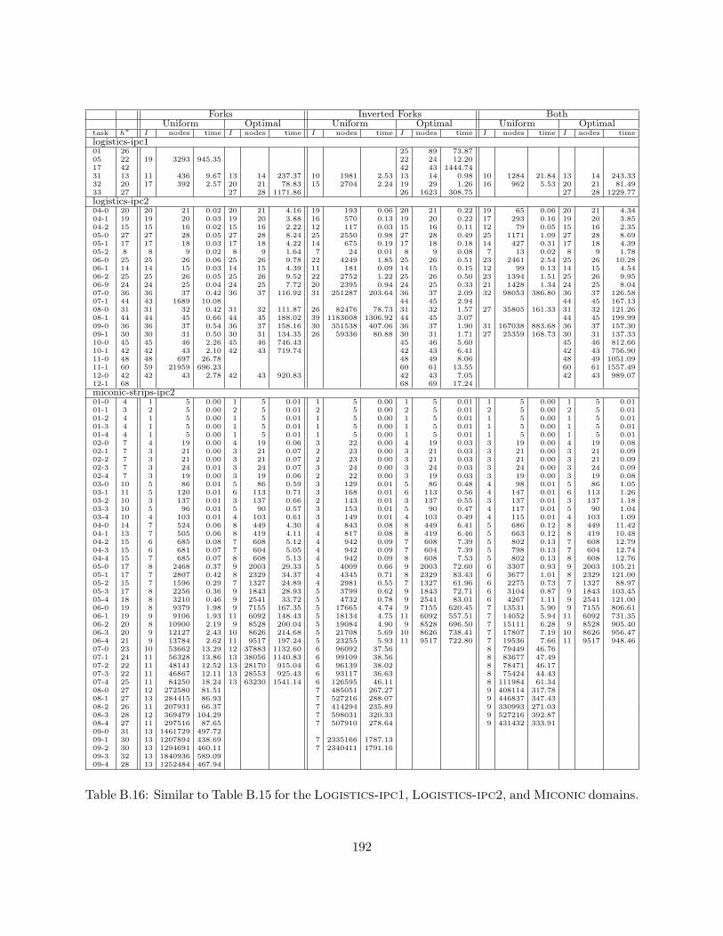
Forks Inverted Forks BothUniform Optimal Uniform Optimal Uniform Optimal
task h∗ I nodes time I nodes time I nodes time I nodes time I nodes time I nodes time
logistics-ipc101 26 25 89 73.8705 22 19 3293 945.35 22 24 12.2017 42 42 43 1444.7431 13 11 436 9.67 13 14 237.37 10 1981 2.53 13 14 0.98 10 1284 21.84 13 14 243.3332 20 17 392 2.57 20 21 78.83 15 2704 2.24 19 29 1.26 16 962 5.53 20 21 81.4933 27 27 28 1171.86 26 1623 308.75 27 28 1229.77
logistics-ipc204-0 20 20 21 0.02 20 21 4.16 19 193 0.06 20 21 0.22 19 65 0.06 20 21 4.3404-1 19 19 20 0.03 19 20 3.88 16 570 0.13 19 20 0.22 17 293 0.16 19 20 3.8504-2 15 15 16 0.02 15 16 2.22 12 117 0.03 15 16 0.11 12 79 0.05 15 16 2.3505-0 27 27 28 0.05 27 28 8.24 25 2550 0.98 27 28 0.49 25 1171 1.09 27 28 8.6905-1 17 17 18 0.03 17 18 4.22 14 675 0.19 17 18 0.18 14 427 0.31 17 18 4.3905-2 8 8 9 0.02 8 9 1.64 7 24 0.01 8 9 0.08 7 13 0.02 8 9 1.7806-0 25 25 26 0.06 25 26 9.78 22 4249 1.85 25 26 0.51 23 2461 2.54 25 26 10.2806-1 14 14 15 0.03 14 15 4.39 11 181 0.09 14 15 0.15 12 99 0.13 14 15 4.5406-2 25 25 26 0.05 25 26 9.52 22 2752 1.22 25 26 0.50 23 1394 1.51 25 26 9.9506-9 24 24 25 0.04 24 25 7.72 20 2395 0.94 24 25 0.33 21 1428 1.34 24 25 8.0407-0 36 36 37 0.42 36 37 116.92 31 251287 203.64 36 37 2.09 32 98053 386.80 36 37 126.5807-1 44 43 1689 10.08 44 45 2.94 44 45 167.1308-0 31 31 32 0.42 31 32 111.87 26 82476 78.73 31 32 1.57 27 35805 161.33 31 32 121.2608-1 44 44 45 0.66 44 45 188.02 39 1183608 1306.92 44 45 3.07 44 45 199.9909-0 36 36 37 0.54 36 37 158.16 30 351538 407.06 36 37 1.90 31 167038 883.68 36 37 157.3009-1 30 30 31 0.50 30 31 134.35 26 59336 80.88 30 31 1.71 27 25359 168.73 30 31 137.3310-0 45 45 46 2.26 45 46 746.43 45 46 5.60 45 46 812.6610-1 42 42 43 2.10 42 43 719.74 42 43 6.41 42 43 756.9011-0 48 48 697 26.78 48 49 8.06 48 49 1051.0911-1 60 59 21959 696.23 60 61 13.55 60 61 1557.4912-0 42 42 43 2.78 42 43 920.83 42 43 7.05 42 43 989.0712-1 68 68 69 17.24
miconic-strips-ipc201-0 4 1 5 0.00 1 5 0.01 1 5 0.00 1 5 0.01 1 5 0.00 1 5 0.0101-1 3 2 5 0.00 2 5 0.01 2 5 0.00 2 5 0.01 2 5 0.00 2 5 0.0101-2 4 1 5 0.00 1 5 0.01 1 5 0.00 1 5 0.01 1 5 0.00 1 5 0.0101-3 4 1 5 0.00 1 5 0.01 1 5 0.00 1 5 0.01 1 5 0.00 1 5 0.0101-4 4 1 5 0.00 1 5 0.01 1 5 0.00 1 5 0.01 1 5 0.00 1 5 0.0102-0 7 4 19 0.00 4 19 0.06 3 22 0.00 4 19 0.03 3 19 0.00 4 19 0.0802-1 7 3 21 0.00 3 21 0.07 2 23 0.00 3 21 0.03 3 21 0.00 3 21 0.0902-2 7 3 21 0.00 3 21 0.07 2 23 0.00 3 21 0.03 3 21 0.00 3 21 0.0902-3 7 3 24 0.01 3 24 0.07 3 24 0.00 3 24 0.03 3 24 0.00 3 24 0.0902-4 7 3 19 0.00 3 19 0.06 2 22 0.00 3 19 0.03 3 19 0.00 3 19 0.0803-0 10 5 86 0.01 5 86 0.59 3 129 0.01 5 86 0.48 4 98 0.01 5 86 1.0503-1 11 5 120 0.01 6 113 0.71 3 168 0.01 6 113 0.56 4 147 0.01 6 113 1.2603-2 10 3 137 0.01 3 137 0.66 2 143 0.01 3 137 0.55 3 137 0.01 3 137 1.1803-3 10 5 96 0.01 5 90 0.57 3 153 0.01 5 90 0.47 4 117 0.01 5 90 1.0403-4 10 4 103 0.01 4 103 0.61 3 149 0.01 4 103 0.49 4 115 0.01 4 103 1.0904-0 14 7 524 0.06 8 449 4.30 4 843 0.08 8 449 6.41 5 686 0.12 8 449 11.4204-1 13 7 505 0.06 8 419 4.11 4 817 0.08 8 419 6.46 5 663 0.12 8 419 10.4804-2 15 6 685 0.08 7 608 5.12 4 942 0.09 7 608 7.39 5 802 0.13 7 608 12.7904-3 15 6 681 0.07 7 604 5.05 4 942 0.09 7 604 7.39 5 798 0.13 7 604 12.7404-4 15 7 685 0.07 8 608 5.13 4 942 0.09 8 608 7.53 5 802 0.13 8 608 12.7605-0 17 8 2468 0.37 9 2003 29.33 5 4009 0.66 9 2003 72.60 6 3307 0.93 9 2003 105.2105-1 17 7 2807 0.42 8 2329 34.37 4 4345 0.71 8 2329 83.43 6 3677 1.01 8 2329 121.0005-2 15 7 1596 0.29 7 1327 24.89 4 2981 0.55 7 1327 61.96 6 2275 0.73 7 1327 88.9705-3 17 8 2256 0.36 9 1843 28.93 5 3799 0.62 9 1843 72.71 6 3104 0.87 9 1843 103.4505-4 18 8 3210 0.46 9 2541 33.72 5 4732 0.78 9 2541 83.01 6 4267 1.11 9 2541 121.0006-0 19 8 9379 1.98 9 7155 167.35 5 17665 4.74 9 7155 620.45 7 13531 5.90 9 7155 806.6106-1 19 9 9106 1.93 11 6092 148.43 5 18134 4.75 11 6092 557.51 7 14052 5.94 11 6092 731.3506-2 20 8 10900 2.19 9 8528 200.04 5 19084 4.90 9 8528 696.50 7 15111 6.28 9 8528 905.4006-3 20 9 12127 2.43 10 8626 214.68 5 21708 5.69 10 8626 738.41 7 17807 7.19 10 8626 956.4706-4 21 9 13784 2.62 11 9517 197.24 5 23255 5.93 11 9517 722.80 7 19536 7.66 11 9517 948.4607-0 23 10 53662 13.29 12 37883 1132.60 6 96092 37.56 8 79449 46.7607-1 24 11 56328 13.86 13 38056 1140.83 6 99109 38.56 8 83677 47.4907-2 22 11 48141 12.52 13 28170 915.04 6 96139 38.02 8 78471 46.1707-3 22 11 46867 12.11 13 28553 925.43 6 93117 36.63 8 75424 44.4307-4 25 11 84250 18.24 13 63230 1541.14 6 126595 46.11 8 111984 61.3408-0 27 12 272580 81.51 7 485051 267.27 9 408114 317.7808-1 27 13 284415 86.93 7 527216 288.07 9 446837 347.4308-2 26 11 207931 66.37 7 414294 235.89 9 330993 271.0308-3 28 12 369479 104.29 7 598031 320.33 9 527216 392.8708-4 27 11 297516 87.65 7 507910 278.64 9 431432 333.9109-0 31 13 1461729 497.7209-1 30 13 1207894 438.69 7 2335166 1787.1309-2 30 13 1294691 460.11 7 2340411 1791.1609-3 32 13 1840936 589.0909-4 28 13 1252484 467.94
Table B.16: Similar to Table B.15 for the Logistics-ipc1, Logistics-ipc2, and Miconic domains.
192
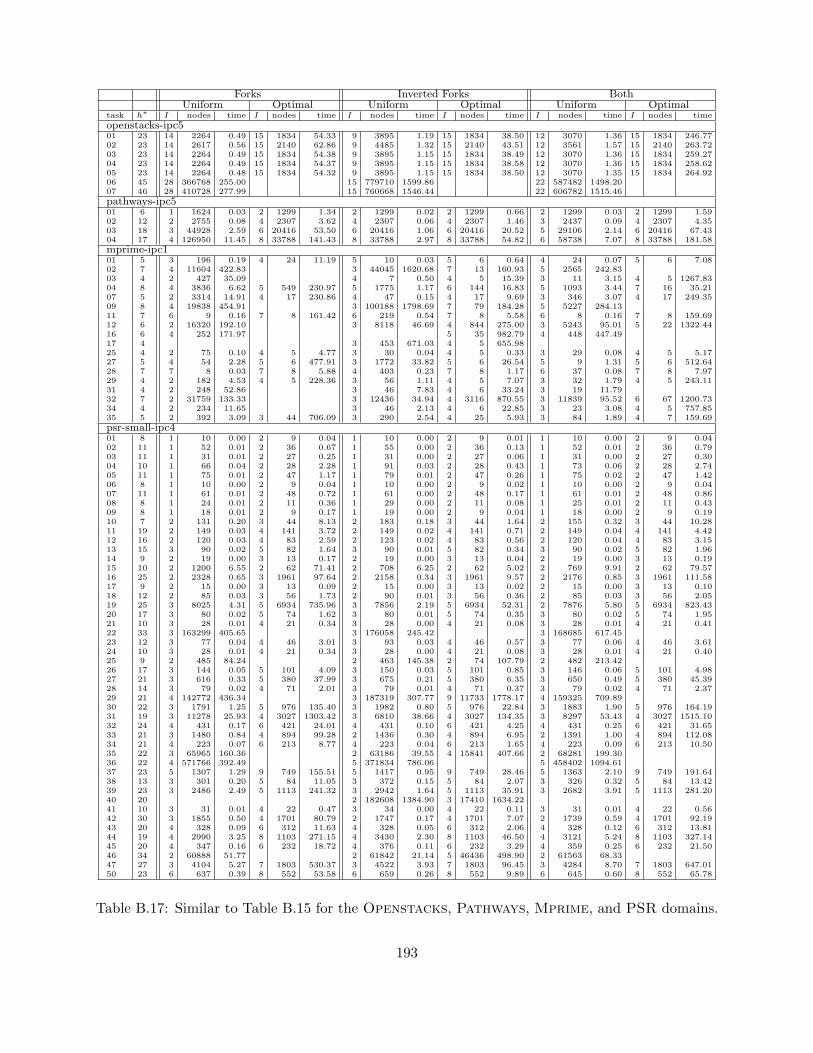
Forks Inverted Forks BothUniform Optimal Uniform Optimal Uniform Optimal
task h∗ I nodes time I nodes time I nodes time I nodes time I nodes time I nodes time
openstacks-ipc501 23 14 2264 0.49 15 1834 54.33 9 3895 1.19 15 1834 38.50 12 3070 1.36 15 1834 246.7702 23 14 2617 0.56 15 2140 62.86 9 4485 1.32 15 2140 43.51 12 3561 1.57 15 2140 263.7203 23 14 2264 0.49 15 1834 54.38 9 3895 1.15 15 1834 38.49 12 3070 1.36 15 1834 259.2704 23 14 2264 0.49 15 1834 54.37 9 3895 1.15 15 1834 38.58 12 3070 1.36 15 1834 258.6205 23 14 2264 0.48 15 1834 54.32 9 3895 1.15 15 1834 38.50 12 3070 1.35 15 1834 264.9206 45 28 366768 255.00 15 779710 1599.86 22 587482 1498.2007 46 28 410728 277.99 15 760668 1546.44 22 606782 1515.46
pathways-ipc501 6 1 1624 0.03 2 1299 1.34 2 1299 0.02 2 1299 0.66 2 1299 0.03 2 1299 1.5902 12 2 2755 0.08 4 2307 3.62 4 2307 0.06 4 2307 1.46 3 2437 0.09 4 2307 4.3503 18 3 44928 2.59 6 20416 53.50 6 20416 1.06 6 20416 20.52 5 29106 2.14 6 20416 67.4304 17 4 126950 11.45 8 33788 141.43 8 33788 2.97 8 33788 54.82 6 58738 7.07 8 33788 181.58
mprime-ipc101 5 3 196 0.19 4 24 11.19 5 10 0.03 5 6 0.64 4 24 0.07 5 6 7.0802 7 4 11604 422.83 3 44045 1620.68 7 13 160.93 5 2565 242.8303 4 2 427 35.09 4 7 0.50 4 5 15.39 3 11 3.15 4 5 1267.8304 8 4 3836 6.62 5 549 230.97 5 1775 1.17 6 144 16.83 5 1093 3.44 7 16 35.2107 5 2 3314 14.91 4 17 230.86 4 47 0.15 4 17 9.69 3 346 3.07 4 17 249.3509 8 4 19838 454.91 3 100188 1798.69 7 79 184.28 5 5227 284.1311 7 6 9 0.16 7 8 161.42 6 219 0.54 7 8 5.58 6 8 0.16 7 8 159.6912 6 2 16320 192.10 3 8118 46.69 4 844 275.00 3 5243 95.01 5 22 1322.4416 6 4 252 171.97 5 35 982.79 4 448 447.4917 4 3 453 671.03 4 5 655.9825 4 2 75 0.10 4 5 4.77 3 30 0.04 4 5 0.33 3 29 0.08 4 5 5.1727 5 4 54 2.28 5 6 477.91 3 1772 33.82 5 6 26.54 5 9 1.31 5 6 512.6428 7 7 8 0.03 7 8 5.88 4 403 0.23 7 8 1.17 6 37 0.08 7 8 7.9729 4 2 182 4.53 4 5 228.36 3 56 1.11 4 5 7.07 3 32 1.79 4 5 243.1131 4 2 248 52.86 3 46 7.83 4 6 33.24 3 19 11.7932 7 2 31759 133.33 3 12436 34.94 4 3116 870.55 3 11839 95.52 6 67 1200.7334 4 2 234 11.65 3 46 2.13 4 6 22.85 3 23 3.08 4 5 757.8535 5 2 392 3.09 3 44 706.09 3 290 2.54 4 25 5.93 3 84 1.89 4 7 159.69
psr-small-ipc401 8 1 10 0.00 2 9 0.04 1 10 0.00 2 9 0.01 1 10 0.00 2 9 0.0402 11 1 52 0.01 2 36 0.67 1 55 0.00 2 36 0.13 1 52 0.01 2 36 0.7903 11 1 31 0.01 2 27 0.25 1 31 0.00 2 27 0.06 1 31 0.00 2 27 0.3004 10 1 66 0.04 2 28 2.28 1 91 0.03 2 28 0.43 1 73 0.06 2 28 2.7405 11 1 75 0.01 2 47 1.17 1 79 0.01 2 47 0.26 1 75 0.02 2 47 1.4206 8 1 10 0.00 2 9 0.04 1 10 0.00 2 9 0.02 1 10 0.00 2 9 0.0407 11 1 61 0.01 2 48 0.72 1 61 0.00 2 48 0.17 1 61 0.01 2 48 0.8608 8 1 24 0.01 2 11 0.36 1 29 0.00 2 11 0.08 1 25 0.01 2 11 0.4309 8 1 18 0.01 2 9 0.17 1 19 0.00 2 9 0.04 1 18 0.00 2 9 0.1910 7 2 131 0.20 3 44 8.13 2 183 0.18 3 44 1.64 2 155 0.32 3 44 10.2811 19 2 149 0.03 4 141 3.72 2 149 0.02 4 141 0.71 2 149 0.04 4 141 4.4212 16 2 120 0.03 4 83 2.59 2 123 0.02 4 83 0.56 2 120 0.04 4 83 3.1513 15 3 90 0.02 5 82 1.64 3 90 0.01 5 82 0.34 3 90 0.02 5 82 1.9614 9 2 19 0.00 3 13 0.17 2 19 0.00 3 13 0.04 2 19 0.00 3 13 0.1915 10 2 1200 6.55 2 62 71.41 2 708 6.25 2 62 5.02 2 769 9.91 2 62 79.5716 25 2 2328 0.65 3 1961 97.64 2 2158 0.34 3 1961 9.57 2 2176 0.85 3 1961 111.5817 9 2 15 0.00 3 13 0.09 2 15 0.00 3 13 0.02 2 15 0.00 3 13 0.1018 12 2 85 0.03 3 56 1.73 2 90 0.01 3 56 0.36 2 85 0.03 3 56 2.0519 25 3 8025 4.31 5 6934 735.96 3 7856 2.19 5 6934 52.31 2 7876 5.80 5 6934 823.4320 17 3 80 0.02 5 74 1.62 3 80 0.01 5 74 0.35 3 80 0.02 5 74 1.9521 10 3 28 0.01 4 21 0.34 3 28 0.00 4 21 0.08 3 28 0.01 4 21 0.4122 33 3 163299 405.65 3 176058 245.42 3 168685 617.4523 12 3 77 0.04 4 46 3.01 3 93 0.03 4 46 0.57 3 77 0.06 4 46 3.6124 10 3 28 0.01 4 21 0.34 3 28 0.00 4 21 0.08 3 28 0.01 4 21 0.4025 9 2 485 84.24 2 463 145.38 2 74 107.79 2 482 213.4226 17 3 144 0.05 5 101 4.09 3 150 0.03 5 101 0.85 3 146 0.06 5 101 4.9827 21 3 616 0.33 5 380 37.99 3 675 0.21 5 380 6.35 3 650 0.49 5 380 45.3928 14 3 79 0.02 4 71 2.01 3 79 0.01 4 71 0.37 3 79 0.02 4 71 2.3729 21 4 142772 436.34 3 187319 307.77 9 11733 1778.17 4 159325 709.8930 22 3 1791 1.25 5 976 135.40 3 1982 0.80 5 976 22.84 3 1883 1.90 5 976 164.1931 19 3 11278 25.93 4 3027 1303.42 3 6810 38.66 4 3027 134.35 3 8297 53.43 4 3027 1515.1032 24 4 431 0.17 6 421 24.01 4 431 0.10 6 421 4.25 4 431 0.25 6 421 31.6533 21 3 1480 0.84 4 894 99.28 2 1436 0.30 4 894 6.95 2 1391 1.00 4 894 112.0834 21 4 223 0.07 6 213 8.77 4 223 0.04 6 213 1.65 4 223 0.09 6 213 10.5035 22 3 65965 160.36 2 63186 39.55 4 15841 407.66 2 68281 199.3036 22 4 571766 392.49 5 371834 786.06 5 458402 1094.6137 23 5 1307 1.29 9 749 155.51 5 1417 0.95 9 749 28.46 5 1363 2.10 9 749 191.6438 13 3 301 0.20 5 84 11.05 3 372 0.15 5 84 2.07 3 326 0.32 5 84 13.4239 23 3 2486 2.49 5 1113 241.32 3 2942 1.64 5 1113 35.91 3 2682 3.91 5 1113 281.2040 20 2 182608 1384.90 3 17410 1634.2241 10 3 31 0.01 4 22 0.47 3 34 0.00 4 22 0.11 3 31 0.01 4 22 0.5642 30 3 1855 0.50 4 1701 80.79 2 1747 0.17 4 1701 7.07 2 1739 0.59 4 1701 92.1943 20 4 328 0.09 6 312 11.63 4 328 0.05 6 312 2.06 4 328 0.12 6 312 13.8144 19 4 2990 3.25 8 1103 271.15 4 3430 2.30 8 1103 46.50 4 3121 5.24 8 1103 327.1445 20 4 347 0.16 6 232 18.72 4 376 0.11 6 232 3.29 4 359 0.25 6 232 21.5046 34 2 60888 51.77 2 61842 21.14 5 46436 498.90 2 61563 68.3347 27 3 4104 5.27 7 1803 530.37 3 4522 3.93 7 1803 96.45 3 4284 8.70 7 1803 647.0150 23 6 637 0.39 8 552 53.58 6 659 0.26 8 552 9.89 6 645 0.60 8 552 65.78
Table B.17: Similar to Table B.15 for the Openstacks, Pathways, Mprime, and PSR domains.
193
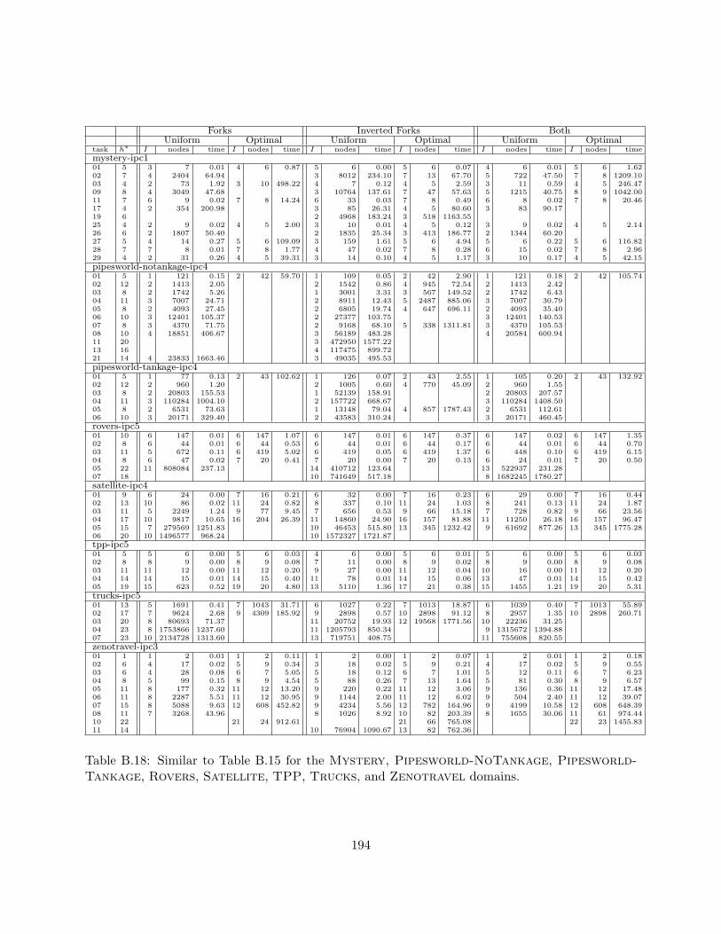
Forks Inverted Forks BothUniform Optimal Uniform Optimal Uniform Optimal
task h∗ I nodes time I nodes time I nodes time I nodes time I nodes time I nodes time
mystery-ipc101 5 3 7 0.01 4 6 0.87 5 6 0.00 5 6 0.07 4 6 0.01 5 6 1.6202 7 4 2404 64.94 3 8012 234.10 7 13 67.70 5 722 47.50 7 8 1209.1003 4 2 73 1.92 3 10 498.22 4 7 0.12 4 5 2.59 3 11 0.59 4 5 246.4709 8 4 3049 47.68 3 10764 137.61 7 47 57.63 5 1215 40.75 8 9 1042.0011 7 6 9 0.02 7 8 14.24 6 33 0.03 7 8 0.49 6 8 0.02 7 8 20.4617 4 2 354 200.98 3 85 26.31 4 5 80.60 3 83 90.1719 6 2 4968 183.24 3 518 1163.5525 4 2 9 0.02 4 5 2.00 3 10 0.01 4 5 0.12 3 9 0.02 4 5 2.1426 6 2 1807 50.40 2 1835 25.34 3 413 186.77 2 1344 60.2027 5 4 14 0.27 5 6 109.09 3 159 1.61 5 6 4.94 5 6 0.22 5 6 116.8228 7 7 8 0.01 7 8 1.77 4 47 0.02 7 8 0.28 6 15 0.02 7 8 2.9629 4 2 31 0.26 4 5 39.31 3 14 0.10 4 5 1.17 3 10 0.17 4 5 42.15
pipesworld-notankage-ipc401 5 1 121 0.15 2 42 59.70 1 109 0.05 2 42 2.90 1 121 0.18 2 42 105.7402 12 2 1413 2.05 2 1542 0.86 4 945 72.54 2 1413 2.4203 8 2 1742 5.26 1 3001 3.31 3 567 149.52 2 1742 6.4304 11 3 7007 24.71 2 8911 12.43 5 2487 885.06 3 7007 30.7905 8 2 4093 27.45 2 6805 19.74 4 647 696.11 2 4093 35.4006 10 3 12401 105.37 2 27377 103.75 3 12401 140.5307 8 3 4370 71.75 2 9168 68.10 5 338 1311.81 3 4370 105.5308 10 4 18851 406.67 3 56189 483.28 4 20584 600.9411 20 3 472950 1577.2213 16 4 117475 899.7221 14 4 23833 1663.46 3 49035 495.53
pipesworld-tankage-ipc401 5 1 77 0.13 2 43 102.62 1 126 0.07 2 43 2.55 1 105 0.20 2 43 132.9202 12 2 960 1.20 2 1005 0.60 4 770 45.09 2 960 1.5503 8 2 20803 155.53 1 52139 158.91 2 20803 207.5704 11 3 110284 1004.10 2 157722 668.67 3 110284 1408.5005 8 2 6531 73.63 1 13148 79.04 4 857 1787.43 2 6531 112.6106 10 3 20171 329.40 2 43583 310.24 3 20171 460.45
rovers-ipc501 10 6 147 0.01 6 147 1.07 6 147 0.01 6 147 0.37 6 147 0.02 6 147 1.3502 8 6 44 0.01 6 44 0.53 6 44 0.01 6 44 0.17 6 44 0.01 6 44 0.7003 11 5 672 0.11 6 419 5.02 6 419 0.05 6 419 1.37 6 448 0.10 6 419 6.1504 8 6 47 0.02 7 20 0.41 7 20 0.00 7 20 0.13 6 24 0.01 7 20 0.5005 22 11 808084 237.13 14 410712 123.64 13 522937 231.2807 18 10 741649 517.18 8 1682245 1780.27
satellite-ipc401 9 6 24 0.00 7 16 0.21 6 32 0.00 7 16 0.23 6 29 0.00 7 16 0.4402 13 10 86 0.02 11 24 0.82 8 337 0.10 11 24 1.03 8 241 0.13 11 24 1.8703 11 5 2249 1.24 9 77 9.45 7 656 0.53 9 66 15.18 7 728 0.82 9 66 23.5604 17 10 9817 10.65 16 204 26.39 11 14860 24.90 16 157 81.88 11 11250 26.18 16 157 96.4705 15 7 279569 1251.83 10 46453 515.80 13 345 1232.42 9 61692 877.26 13 345 1775.2806 20 10 1496577 968.24 10 1572327 1721.87
tpp-ipc501 5 5 6 0.00 5 6 0.03 4 6 0.00 5 6 0.01 5 6 0.00 5 6 0.0302 8 8 9 0.00 8 9 0.08 7 11 0.00 8 9 0.02 8 9 0.00 8 9 0.0803 11 11 12 0.00 11 12 0.20 9 27 0.00 11 12 0.04 10 16 0.00 11 12 0.2004 14 14 15 0.01 14 15 0.40 11 78 0.01 14 15 0.06 13 47 0.01 14 15 0.4205 19 15 623 0.52 19 20 4.80 13 5110 1.36 17 21 0.38 15 1455 1.21 19 20 5.31
trucks-ipc501 13 5 1691 0.41 7 1043 31.71 6 1027 0.22 7 1013 18.87 6 1039 0.40 7 1013 55.8902 17 7 9624 2.68 9 4309 185.92 9 2898 0.57 10 2898 91.12 8 2957 1.35 10 2898 260.7103 20 8 80693 71.37 11 20752 19.93 12 19568 1771.56 10 22236 31.2504 23 8 1753866 1237.60 11 1205793 850.34 9 1315672 1394.8807 23 10 2134728 1313.60 13 719751 408.75 11 755608 820.55
zenotravel-ipc301 1 1 2 0.01 1 2 0.11 1 2 0.00 1 2 0.07 1 2 0.01 1 2 0.1802 6 4 17 0.02 5 9 0.34 3 18 0.02 5 9 0.21 4 17 0.02 5 9 0.5503 6 4 28 0.08 6 7 5.05 5 18 0.12 6 7 1.01 5 12 0.11 6 7 6.2304 8 5 99 0.15 8 9 4.54 5 88 0.26 7 13 1.64 5 81 0.30 8 9 6.5705 11 8 177 0.32 11 12 13.20 9 220 0.22 11 12 3.06 9 136 0.36 11 12 17.4806 11 8 2287 5.51 11 12 30.95 9 1144 2.00 11 12 6.02 9 504 2.40 11 12 39.0707 15 8 5088 9.63 12 608 452.82 9 4234 5.56 12 782 164.96 9 4199 10.58 12 608 648.3908 11 7 3268 43.96 8 1026 8.92 10 82 203.39 8 1655 30.06 11 61 974.4410 22 21 24 912.61 21 66 765.08 22 23 1455.8311 14 10 76904 1090.67 13 82 762.36
Table B.18: Similar to Table B.15 for the Mystery, Pipesworld-NoTankage, Pipesworld-Tankage, Rovers, Satellite, TPP, Trucks, and Zenotravel domains.
194
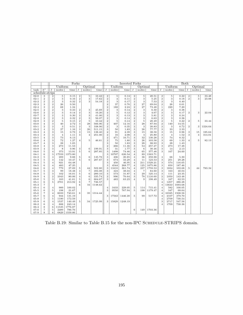
Forks Inverted Forks BothUniform Optimal Uniform Optimal Uniform Optimal
task h∗ I nodes time I nodes time I nodes time I nodes time I nodes time I nodes time
schedule-strips02-0 3 2 5 0.15 2 5 10.42 2 5 0.14 2 5 20.51 2 5 0.22 2 5 33.4802-1 2 2 3 0.16 2 3 17.62 2 4 0.11 2 3 5.25 2 3 0.18 2 3 23.8802-2 2 2 3 0.32 2 3 54.18 2 3 0.17 2 3 7.53 2 3 0.4002-3 3 2 26 0.50 2 37 0.76 2 27 69.04 2 26 0.6102-4 3 2 68 1.34 2 188 2.24 2 27 73.48 1 220 7.2002-5 2 2 3 0.33 2 3 45.69 2 3 0.14 2 3 6.30 2 3 0.3802-6 2 2 3 0.14 2 3 16.20 2 5 0.12 2 3 4.67 2 3 0.17 2 3 22.0402-7 2 2 3 0.30 2 3 41.00 2 3 0.13 2 3 5.81 2 3 0.3402-8 2 2 3 0.32 2 3 56.07 2 3 0.14 2 3 6.63 2 3 0.3802-9 3 2 5 0.15 2 5 10.42 2 5 0.14 2 5 20.49 2 5 0.22 2 5 33.4403-0 4 3 40 2.72 3 28 566.96 2 407 12.16 3 28 87.94 2 140 14.5503-1 2 2 3 0.51 2 3 108.90 2 3 0.35 2 3 20.83 2 3 0.72 2 3 1324.6403-2 4 3 27 1.16 3 26 511.15 3 50 1.83 3 26 77.77 3 33 2.3303-3 4 3 15 0.79 3 15 138.40 2 91 2.39 3 15 38.58 3 15 0.96 3 15 185.6403-4 3 3 4 1.11 3 4 251.00 2 16 2.08 3 4 25.80 3 4 1.52 3 4 314.0103-5 4 3 73 6.13 2 471 16.71 3 32 130.28 3 74 8.3203-6 4 3 72 1.27 4 5 46.61 2 75 1.80 3 26 103.58 3 69 1.33 4 5 82.1303-7 4 3 28 1.05 3 50 1.83 3 28 98.93 3 28 1.4303-8 4 3 273 11.53 2 266 11.46 3 54 257.27 3 273 17.4803-9 4 3 8 0.96 3 6 199.91 3 31 1.77 3 6 30.46 3 14 2.1304-0 5 4 373 13.91 5 6 287.85 3 1498 74.46 4 65 377.48 3 167 24.6004-1 6 3 17559 1373.80 3 10707 626.54 4 89 1563.7104-2 5 4 209 9.88 5 6 145.78 3 406 20.85 4 36 259.88 4 66 5.3004-3 5 3 142 10.47 5 6 287.67 3 674 33.29 4 11 123.53 3 251 29.2804-4 5 4 921 64.48 3 450 46.95 4 211 1529.21 3 574 116.6504-5 6 4 483 47.25 3 4544 268.77 4 125 1675.86 3 850 187.4604-6 6 4 779 27.09 5 44 502.80 3 11610 361.74 4 237 1759.53 3 1834 102.68 5 44 783.3404-7 5 3 99 18.48 4 7 494.08 3 424 38.04 4 7 84.60 3 163 40.0404-8 5 3 102 16.01 5 6 289.10 3 573 31.87 4 29 125.14 3 111 23.3504-9 4 2 1043 80.06 4 6 335.74 2 996 76.64 3 78 1116.60 2 1050 143.4805-0 5 3 163 41.61 5 6 664.67 3 483 63.23 4 9 198.49 3 167 62.5305-1 6 5 2701 213.92 6 7 726.57 4 1257 286.2805-3 7 6 16 1148.62 4 13622 1693.6805-4 6 4 989 100.02 4 3433 229.05 5 114 715.41 4 582 100.0505-5 6 5 198 21.67 3 9550 767.94 5 198 1179.47 4 347 68.6405-6 7 4 6033 743.61 6 35 1314.44 4 10325 1508.5605-7 6 4 944 131.19 3 17562 1446.20 5 99 517.72 4 2107 379.7005-8 7 5 1190 172.59 4 2709 730.5405-9 6 4 1537 140.49 5 34 1725.99 3 15829 1248.19 3 2717 547.5606-2 6 4 888 243.14 4 1709 730.3606-4 8 6 11535 1776.8707-0 7 5 2489 786.76 6 149 1703.3607-9 8 6 6829 1559.86
Table B.19: Similar to Table B.15 for the non-IPC Schedule-STRIPS domain.
195
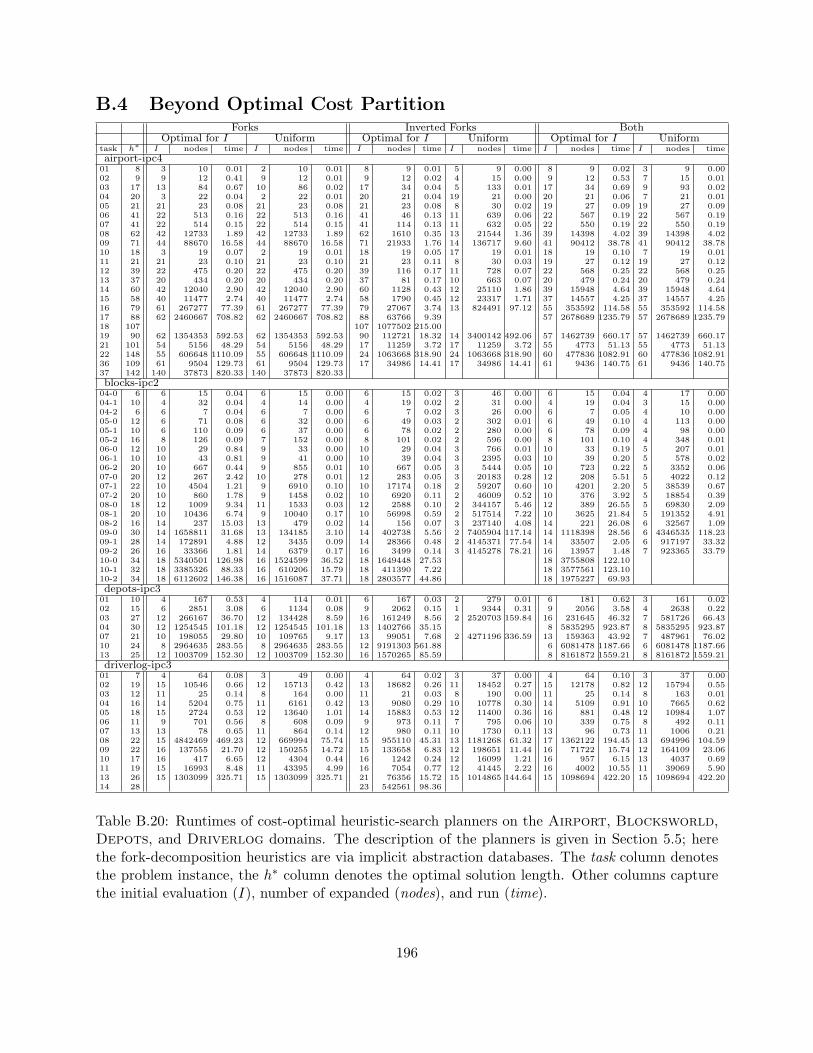
B.4 Beyond Optimal Cost PartitionForks Inverted Forks Both
Optimal for I Uniform Optimal for I Uniform Optimal for I Uniformtask h∗ I nodes time I nodes time I nodes time I nodes time I nodes time I nodes time
airport-ipc401 8 3 10 0.01 2 10 0.01 8 9 0.01 5 9 0.00 8 9 0.02 3 9 0.0002 9 9 12 0.41 9 12 0.01 9 12 0.02 4 15 0.00 9 12 0.53 7 15 0.0103 17 13 84 0.67 10 86 0.02 17 34 0.04 5 133 0.01 17 34 0.69 9 93 0.0204 20 3 22 0.04 2 22 0.01 20 21 0.04 19 21 0.00 20 21 0.06 7 21 0.0105 21 21 23 0.08 21 23 0.08 21 23 0.08 8 30 0.02 19 27 0.09 19 27 0.0906 41 22 513 0.16 22 513 0.16 41 46 0.13 11 639 0.06 22 567 0.19 22 567 0.1907 41 22 514 0.15 22 514 0.15 41 114 0.13 11 632 0.05 22 550 0.19 22 550 0.1908 62 42 12733 1.89 42 12733 1.89 62 1610 0.35 13 21544 1.36 39 14398 4.02 39 14398 4.0209 71 44 88670 16.58 44 88670 16.58 71 21933 1.76 14 136717 9.60 41 90412 38.78 41 90412 38.7810 18 3 19 0.07 2 19 0.01 18 19 0.05 17 19 0.01 18 19 0.10 7 19 0.0111 21 21 23 0.10 21 23 0.10 21 23 0.11 8 30 0.03 19 27 0.12 19 27 0.1212 39 22 475 0.20 22 475 0.20 39 116 0.17 11 728 0.07 22 568 0.25 22 568 0.2513 37 20 434 0.20 20 434 0.20 37 81 0.17 10 663 0.07 20 479 0.24 20 479 0.2414 60 42 12040 2.90 42 12040 2.90 60 1128 0.43 12 25110 1.86 39 15948 4.64 39 15948 4.6415 58 40 11477 2.74 40 11477 2.74 58 1790 0.45 12 23317 1.71 37 14557 4.25 37 14557 4.2516 79 61 267277 77.39 61 267277 77.39 79 27067 3.74 13 824491 97.12 55 353592 114.58 55 353592 114.5817 88 62 2460667 708.82 62 2460667 708.82 88 63766 9.39 57 2678689 1235.79 57 2678689 1235.7918 107 107 1077502 215.0019 90 62 1354353 592.53 62 1354353 592.53 90 112721 18.32 14 3400142 492.06 57 1462739 660.17 57 1462739 660.1721 101 54 5156 48.29 54 5156 48.29 17 11259 3.72 17 11259 3.72 55 4773 51.13 55 4773 51.1322 148 55 606648 1110.09 55 606648 1110.09 24 1063668 318.90 24 1063668 318.90 60 477836 1082.91 60 477836 1082.9136 109 61 9504 129.73 61 9504 129.73 17 34986 14.41 17 34986 14.41 61 9436 140.75 61 9436 140.7537 142 140 37873 820.33 140 37873 820.33
blocks-ipc204-0 6 6 15 0.04 6 15 0.00 6 15 0.02 3 46 0.00 6 15 0.04 4 17 0.0004-1 10 4 32 0.04 4 14 0.00 4 19 0.02 2 31 0.00 4 19 0.04 3 15 0.0004-2 6 6 7 0.04 6 7 0.00 6 7 0.02 3 26 0.00 6 7 0.05 4 10 0.0005-0 12 6 71 0.08 6 32 0.00 6 49 0.03 2 302 0.01 6 49 0.10 4 113 0.0005-1 10 6 110 0.09 6 37 0.00 6 78 0.02 2 280 0.00 6 78 0.09 4 98 0.0005-2 16 8 126 0.09 7 152 0.00 8 101 0.02 2 596 0.00 8 101 0.10 4 348 0.0106-0 12 10 29 0.84 9 33 0.00 10 29 0.04 3 766 0.01 10 33 0.19 5 207 0.0106-1 10 10 43 0.81 9 41 0.00 10 39 0.04 3 2395 0.03 10 39 0.20 5 578 0.0206-2 20 10 667 0.44 9 855 0.01 10 667 0.05 3 5444 0.05 10 723 0.22 5 3352 0.0607-0 20 12 267 2.42 10 278 0.01 12 283 0.05 3 20183 0.28 12 208 5.51 5 4022 0.1207-1 22 10 4504 1.21 9 6910 0.10 10 17174 0.18 2 59207 0.60 10 4201 2.20 5 38539 0.6707-2 20 10 860 1.78 9 1458 0.02 10 6920 0.11 2 46009 0.52 10 376 3.92 5 18854 0.3908-0 18 12 1009 9.34 11 1533 0.03 12 2588 0.10 2 344157 5.46 12 389 26.55 5 69830 2.0908-1 20 10 10436 6.74 9 10040 0.17 10 56998 0.59 2 517514 7.22 10 3625 21.84 5 191352 4.9108-2 16 14 237 15.03 13 479 0.02 14 156 0.07 3 237140 4.08 14 221 26.08 6 32567 1.0909-0 30 14 1658811 31.68 13 134185 3.10 14 402738 5.56 2 7405904 117.14 14 1118398 28.56 6 4346535 118.2309-1 28 14 172891 4.88 12 3435 0.09 14 28366 0.48 2 4145371 77.54 14 33507 2.05 6 917197 33.3209-2 26 16 33366 1.81 14 6379 0.17 16 3499 0.14 3 4145278 78.21 16 13957 1.48 7 923365 33.7910-0 34 18 5340501 126.98 16 1524599 36.52 18 1649448 27.53 18 3755808 122.1010-1 32 18 3385326 88.33 16 610206 15.79 18 411390 7.22 18 3577561 123.1010-2 34 18 6112602 146.38 16 1516087 37.71 18 2803577 44.86 18 1975227 69.93
depots-ipc301 10 4 167 0.53 4 114 0.01 6 167 0.03 2 279 0.01 6 181 0.62 3 161 0.0202 15 6 2851 3.08 6 1134 0.08 9 2062 0.15 1 9344 0.31 9 2056 3.58 4 2638 0.2203 27 12 266167 36.70 12 134428 8.59 16 161249 8.56 2 2520703 159.84 16 231645 46.32 7 581726 66.4304 30 12 1254545 101.18 12 1254545 101.18 13 1402766 35.15 8 5835295 923.87 8 5835295 923.8707 21 10 198055 29.80 10 109765 9.17 13 99051 7.68 2 4271196 336.59 13 159363 43.92 7 487961 76.0210 24 8 2964635 283.55 8 2964635 283.55 12 9191303 561.88 6 6081478 1187.66 6 6081478 1187.6613 25 12 1003709 152.30 12 1003709 152.30 16 1570265 85.59 8 8161872 1559.21 8 8161872 1559.21
driverlog-ipc301 7 4 64 0.08 3 49 0.00 4 64 0.02 3 37 0.00 4 64 0.10 3 37 0.0002 19 15 10546 0.66 12 15713 0.42 13 18682 0.26 11 18452 0.27 15 12178 0.82 12 15794 0.5503 12 11 25 0.14 8 164 0.00 11 21 0.03 8 190 0.00 11 25 0.14 8 163 0.0104 16 14 5204 0.75 11 6161 0.42 13 9080 0.29 10 10778 0.30 14 5109 0.91 10 7665 0.6205 18 15 2724 0.53 12 13640 1.01 14 15883 0.53 12 11400 0.36 16 881 0.48 12 10984 1.0706 11 9 701 0.56 8 608 0.09 9 973 0.11 7 795 0.06 10 339 0.75 8 492 0.1107 13 13 78 0.65 11 864 0.14 12 980 0.11 10 1730 0.11 13 96 0.73 11 1006 0.2108 22 15 4842469 469.23 12 669994 75.74 15 955110 45.31 13 1181268 61.32 17 1362122 194.45 13 694996 104.5909 22 16 137555 21.70 12 150255 14.72 15 133658 6.83 12 198651 11.44 16 71722 15.74 12 164109 23.0610 17 16 417 6.65 12 4304 0.44 16 1242 0.24 12 16099 1.21 16 957 6.15 13 4037 0.6911 19 15 16993 8.48 11 43395 4.99 16 7054 0.77 12 41445 2.22 16 4002 10.55 11 39069 5.9013 26 15 1303099 325.71 15 1303099 325.71 21 76356 15.72 15 1014865 144.64 15 1098694 422.20 15 1098694 422.2014 28 23 542561 98.36
Table B.20: Runtimes of cost-optimal heuristic-search planners on the Airport, Blocksworld,Depots, and Driverlog domains. The description of the planners is given in Section 5.5; herethe fork-decomposition heuristics are via implicit abstraction databases. The task column denotesthe problem instance, the h∗ column denotes the optimal solution length. Other columns capturethe initial evaluation (I), number of expanded (nodes), and run (time).
196
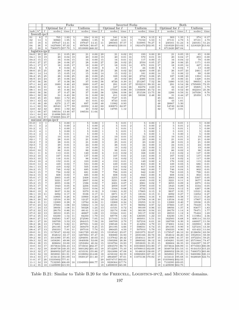
Forks Inverted Forks BothOptimal for I Uniform Optimal for I Uniform Optimal for I Uniform
task h∗ I nodes time I nodes time I nodes time I nodes time I nodes time I nodes time
freecell-ipc301 8 7 705 1.93 5 234 0.10 8 541 0.34 3 974 0.15 8 303 1.35 5 274 0.1702 14 5 30960 1.95 5 30960 1.95 9 42549 4.01 3 75150 5.53 5 37131 4.79 5 37131 4.7903 18 6 197647 14.41 6 197647 14.41 11 280303 37.57 3 533995 78.27 6 240161 51.24 6 240161 51.2404 26 8 1427669 97.22 6 997836 60.67 8 1894652 130.01 3 1921470 232.95 6 1218329 213.02 6 1218329 213.0205 30 8 7369373 557.79 5 6510089 448.22 8 8712420 987.04
logistics-ipc204-0 20 20 21 0.05 20 21 0.00 20 21 0.02 19 193 0.00 20 21 0.05 19 65 0.0004-1 19 19 20 0.04 19 20 0.00 19 20 0.01 16 570 0.01 19 20 0.04 17 293 0.0004-2 15 15 16 0.04 15 16 0.00 15 16 0.01 12 117 0.00 15 16 0.04 12 79 0.0005-0 27 27 28 0.06 27 28 0.00 27 28 0.02 25 2550 0.05 27 28 0.06 25 1171 0.0305-1 17 17 18 0.05 17 18 0.00 17 18 0.01 14 675 0.01 17 18 0.05 14 427 0.0105-2 8 8 9 0.04 8 9 0.00 8 9 0.01 7 24 0.00 8 9 0.04 7 13 0.0006-0 25 25 26 0.06 25 26 0.00 25 26 0.02 22 4249 0.09 25 26 0.07 23 2461 0.0706-1 14 14 15 0.05 14 15 0.00 14 15 0.02 11 181 0.00 14 15 0.06 12 99 0.0006-2 25 25 26 0.06 25 26 0.00 25 169 0.02 22 2752 0.06 25 187 0.08 23 1394 0.0406-9 24 24 25 0.06 24 25 0.00 24 25 0.02 20 2395 0.04 24 25 0.06 21 1428 0.0407-0 36 36 37 0.38 36 37 0.00 36 8726 0.39 31 251287 7.52 36 1480 0.55 32 98053 4.5907-1 44 43 1689 0.46 43 1689 0.07 44 291 0.05 37 3532213 99.33 44 291 0.54 38 1705009 72.3508-0 31 31 32 0.41 31 32 0.00 31 347 0.04 26 82476 2.69 31 32 0.43 27 35805 1.7808-1 44 44 45 0.46 44 45 0.01 44 17554 0.98 39 1183608 45.72 44 45 0.52 40 462244 25.3609-0 36 36 37 0.47 36 37 0.00 36 1296 0.08 30 351538 13.75 36 1206 0.59 31 167038 9.7609-1 30 30 31 0.43 30 31 0.00 30 211 0.03 26 59336 2.48 30 31 0.44 27 25359 1.7310-0 45 45 3421 1.72 45 46 0.01 45 7547 0.55 45 3621 2.1110-1 42 42 253 1.52 42 43 0.01 42 8723 0.63 42 43 1.8111-0 48 48 4279 2.17 48 697 0.09 48 11082 0.93 48 20667 5.3011-1 60 59 20523 3.77 59 21959 2.22 60 630873 62.97 60 54749 12.9812-0 42 42 2041 1.92 42 43 0.02 42 14795 1.12 42 7137 3.0112-1 68 67 106534 13.46 67 106534 11.6413-1 64 63 214096 105.2214-0 58 57 1720905 534.37
miconic-strips-ipc201-0 4 1 5 0.00 1 5 0.00 1 5 0.01 1 5 0.00 1 5 0.01 1 5 0.0001-1 3 2 5 0.00 2 5 0.00 2 5 0.01 2 5 0.00 2 5 0.01 2 5 0.0001-2 4 1 5 0.00 1 5 0.00 1 5 0.01 1 5 0.00 1 5 0.01 1 5 0.0001-3 4 1 5 0.00 1 5 0.00 1 5 0.01 1 5 0.00 1 5 0.01 1 5 0.0001-4 4 1 5 0.01 1 5 0.00 1 5 0.01 1 5 0.00 1 5 0.00 1 5 0.0002-0 7 4 19 0.01 4 19 0.00 4 19 0.01 3 22 0.00 4 19 0.01 3 19 0.0002-1 7 3 28 0.01 3 21 0.00 3 21 0.01 2 23 0.00 3 21 0.01 3 21 0.0002-2 7 3 28 0.01 3 21 0.00 3 25 0.01 2 23 0.00 3 28 0.01 3 21 0.0002-3 7 3 29 0.01 3 24 0.00 3 26 0.01 3 24 0.00 3 24 0.01 3 24 0.0002-4 7 3 26 0.01 3 19 0.00 3 19 0.02 2 22 0.00 3 23 0.01 3 19 0.0003-0 10 5 86 0.01 5 86 0.00 5 96 0.01 3 129 0.00 5 86 0.02 4 98 0.0003-1 11 6 113 0.01 5 120 0.00 6 113 0.02 3 168 0.00 6 113 0.02 4 147 0.0003-2 10 3 167 0.01 3 137 0.00 3 167 0.01 2 143 0.00 3 167 0.02 3 137 0.0003-3 10 5 116 0.01 5 96 0.00 5 116 0.02 3 153 0.00 5 116 0.02 4 117 0.0003-4 10 4 152 0.01 4 103 0.00 4 152 0.01 3 149 0.00 4 176 0.02 4 115 0.0004-0 14 8 449 0.02 7 524 0.00 8 449 0.03 4 843 0.00 8 449 0.03 5 686 0.0104-1 13 8 419 0.02 7 505 0.00 8 419 0.02 4 817 0.00 8 419 0.03 5 663 0.0104-2 15 7 746 0.02 6 685 0.00 7 746 0.04 4 942 0.00 7 746 0.04 5 802 0.0104-3 15 7 756 0.02 6 681 0.00 7 756 0.03 4 942 0.00 7 756 0.03 5 798 0.0104-4 15 8 608 0.02 7 685 0.00 8 608 0.04 4 942 0.00 8 608 0.04 5 802 0.0105-0 17 9 2003 0.05 8 2468 0.03 9 2255 0.07 5 4009 0.03 9 2003 0.09 6 3307 0.0505-1 17 8 3221 0.07 7 2807 0.04 8 3221 0.08 4 4345 0.03 8 3221 0.11 6 3677 0.0605-2 15 7 2055 0.06 7 1596 0.02 7 2401 0.07 4 2981 0.02 7 2055 0.09 6 2275 0.0405-3 17 9 1843 0.05 8 2256 0.03 9 2059 0.07 5 3799 0.03 9 1843 0.09 6 3104 0.0505-4 18 9 3164 0.07 8 3210 0.04 9 3164 0.08 5 4732 0.03 9 3164 0.12 6 4267 0.0606-0 19 9 9637 0.24 8 9379 0.18 9 11061 0.22 5 17665 0.15 9 9637 0.35 7 13531 0.2606-1 19 11 6092 0.17 9 9106 0.17 11 6871 0.17 5 18134 0.15 11 6092 0.27 7 14052 0.2706-2 20 9 10805 0.26 8 10900 0.20 9 12948 0.25 5 19084 0.16 9 10805 0.38 7 15111 0.2806-3 20 10 12534 0.30 9 12127 0.23 10 12534 0.24 5 21708 0.18 10 12534 0.42 7 17807 0.3306-4 21 11 12269 0.28 9 13784 0.24 11 12269 0.24 5 23255 0.19 11 12269 0.40 7 19536 0.3507-0 23 12 37883 1.08 10 53662 1.19 12 46181 0.77 6 96092 0.97 12 37883 1.37 8 79449 1.7607-1 24 13 38056 1.08 11 56328 1.24 13 41531 0.72 6 99109 0.96 13 38056 1.37 8 83677 1.8307-2 22 13 28170 0.86 11 48141 1.10 13 32174 0.60 6 96139 0.94 13 28170 1.14 8 78471 1.7707-3 22 13 28553 0.85 11 46867 1.08 13 31944 0.61 6 93117 0.92 13 28553 1.12 8 75424 1.6907-4 25 13 63230 1.54 11 84250 1.70 13 68778 1.02 6 126595 1.22 13 63230 1.91 8 111984 2.3608-0 27 14 182583 5.87 12 272580 7.05 14 217443 3.53 7 485051 5.51 14 182583 6.68 9 408114 10.5308-1 27 16 160709 5.53 13 284415 7.56 16 160709 2.79 7 527216 6.01 16 160709 6.30 9 446837 11.5808-2 26 13 174001 5.82 11 207931 5.60 13 198548 3.34 7 414294 4.79 13 174001 6.64 9 330993 8.9008-3 28 15 291195 8.87 12 369479 9.25 15 291195 4.66 7 598031 6.74 15 291195 9.90 9 527216 13.3008-4 27 13 256333 7.91 11 297516 7.74 13 286425 4.59 7 507910 5.79 13 256333 8.90 9 431432 11.0409-0 31 15 1178547 42.62 13 1461729 43.82 15 1318542 23.07 7 2491975 32.67 15 1178547 46.10 10 2138656 63.5809-1 30 16 852612 33.17 13 1207894 37.47 16 930890 16.93 7 2335166 30.76 16 852612 36.20 10 1952916 59.3909-2 30 15 1014390 37.85 13 1294691 40.03 15 1137842 20.42 7 2340411 30.97 15 1014390 41.37 10 1972234 59.2509-3 32 16 1458281 49.88 13 1840936 52.68 16 1560206 26.36 7 2889342 38.12 16 1458281 53.85 10 2571844 74.4709-4 28 15 808604 33.00 13 1252484 40.34 15 1016784 18.93 7 2352633 31.35 15 808604 36.35 10 1944297 59.3710-0 33 17 3573644 156.43 14 5716041 202.37 17 4384570 86.73 8 10316603 153.80 17 3573644 168.99 11 8774563 300.0810-1 32 18 3048758 140.35 15 5601282 201.43 18 3712295 75.10 8 10789013 162.69 18 3048758 151.53 11 9144153 315.2310-2 32 17 2680052 127.22 14 4153191 155.86 17 3241896 67.08 8 9148616 138.69 17 2680052 138.35 11 7466572 265.8610-3 34 18 3658921 161.91 15 6108094 214.68 18 4158162 82.59 8 10960203 167.10 18 3658921 173.25 11 9400386 320.1310-4 33 17 4134141 181.00 14 5920127 211.40 17 4864687 97.61 8 11075136 170.82 17 4134141 195.68 11 9448049 322.7411-0 37 20 15335602 777.41 20 16574717 402.63 20 15335602 832.5511-1 34 19 7132395 406.69 16 15349953 668.77 19 9228364 217.74 19 7132395 439.0511-4 35 18 11409090 615.93 18 14888659 345.88 18 11409090 662.75
Table B.21: Similar to Table B.20 for the Freecell, Logistics-ipc2, and Miconic domains.197
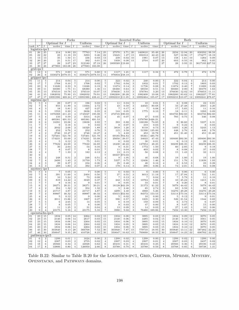
Forks Inverted Forks BothOptimal for I Uniform Optimal for I Uniform Optimal for I Uniform
task h∗ I nodes time I nodes time I nodes time I nodes time I nodes time I nodes time
logistics-ipc101 26 25 214 9.90 22 77763 7.14 25 27570 2.71 20 1469610 95.49 26 2234 12.94 20 830292 98.5905 22 22 23 11.16 19 3293 0.46 22 15645 1.27 15 850312 42.43 22 527 12.96 17 173477 18.1931 13 13 35 1.50 11 436 0.03 13 239 0.02 10 1981 0.07 13 158 1.61 10 1284 0.0932 20 20 21 0.51 17 392 0.01 19 1939 0.08 15 2704 0.07 20 603 0.55 16 962 0.0533 27 27 28 3.07 23 312180 27.19 26 1609589 119.68 27 28 3.93 21 3617185 427.5235 30 26 477883 183.08 26 477883 183.08
grid-ipc101 14 4 571 0.60 4 571 0.60 6 1117 1.21 6 1117 0.34 5 472 0.78 5 472 0.7802 26 6 3330274 1078.55 6 3330274 1078.55 11 976834 158.19
gripper-ipc101 11 5 214 0.04 5 214 0.00 5 222 0.02 3 240 0.00 5 222 0.04 4 214 0.0002 17 7 1768 0.10 7 1768 0.02 7 1792 0.04 3 1832 0.01 7 1792 0.13 6 1803 0.0303 23 9 11626 0.33 9 11626 0.19 9 11674 0.14 3 11736 0.08 9 11674 0.40 7 11689 0.2204 29 11 68380 1.75 11 68380 1.46 11 68460 0.64 3 68558 0.51 11 68460 2.00 8 68479 1.6305 35 13 376510 10.76 13 376510 10.07 13 376630 3.53 3 376784 3.20 13 376630 12.02 10 376653 11.1106 41 15 1982032 75.90 15 1982032 70.91 15 1982200 20.28 3 1982408 19.08 15 1982200 83.62 11 1982227 77.8107 47 17 10091986 469.24 17 10091986 438.41 17 10092210 111.05 3 10092464 105.67 17 10092210 510.07 12 10092241 478.67
mprime-ipc101 5 4 28 0.07 3 196 0.02 5 11 0.04 5 10 0.01 5 6 0.08 4 24 0.0102 7 6 855 11.89 4 11604 2.72 7 43 0.58 3 44045 80.68 7 33 27.48 5 2565 4.2003 4 3 18 5.81 2 427 0.27 4 7 0.17 4 7 0.08 4 17 5.65 3 11 0.1604 8 5 1553 0.20 4 3836 0.22 6 144 0.05 5 1775 0.10 7 18 0.11 5 1093 0.0905 11 6 1076368 211.43 4 1745027 195.08 7 272745 190.03 5 604756 592.60 5 604756 592.6007 5 4 133 0.59 2 3314 0.25 4 45 0.07 4 47 0.03 4 785 0.75 3 346 0.0808 6 2 485381 491.53 2 485381 491.53 2 1376780 1426.2109 8 6 16391 22.06 4 19838 2.92 7 393 0.88 3 100188 74.85 8 9 26.60 5 5227 6.3111 7 7 9 0.18 6 9 0.02 7 8 0.07 6 219 0.03 7 9 0.22 6 8 0.0312 6 3 2042 2.68 2 16320 1.89 4 3818 1.20 3 8118 0.73 5 1405 4.26 3 5243 1.1316 6 4 252 0.76 4 252 0.76 5 115 3.58 2 51590 135.00 4 448 2.76 4 448 2.7617 4 2 2746 10.47 2 2746 10.47 4 5 4.22 3 453 18.78 3 451 21.40 3 451 21.4019 6 2 727401 521.78 2 727401 521.78 3 69185 704.84 2 95361 485.7921 6 2 174221 55.09 2 174221 55.09 3 25650 29.57 2 34022 47.43 2 169400 392.30 2 169400 392.3025 4 4 5 0.12 2 75 0.01 4 6 0.02 3 30 0.01 4 6 0.13 3 29 0.0126 6 2 77622 24.69 2 77622 24.69 3 18430 46.22 2 147854 48.25 2 68239 106.35 2 68239 106.3527 5 5 30 2.64 4 54 0.16 5 9 0.31 3 1772 1.50 5 60 2.85 5 9 0.1828 7 7 8 0.07 7 8 0.01 7 11 0.04 4 403 0.02 7 8 0.08 6 37 0.0229 4 4 7 1.33 2 182 0.12 4 13 0.15 3 56 0.08 4 15 1.43 3 32 0.1130 9 7 69337 373.0331 4 2 248 0.51 2 248 0.51 4 9 1.05 3 46 0.68 3 19 1.00 3 19 1.0032 7 4 2499 1.43 2 31759 1.73 4 5337 0.75 3 12436 1.46 6 151 1.76 3 11839 1.9334 4 3 29 8.37 2 234 0.26 4 29 0.48 3 46 0.16 4 6 6.53 3 23 0.2835 5 3 269 1.83 2 392 0.07 4 178 0.14 3 290 0.06 4 74 2.01 3 84 0.08
mystery-ipc101 5 4 7 0.05 3 7 0.00 5 6 0.02 5 6 0.00 5 6 0.06 4 6 0.0002 7 6 391 11.60 4 2404 0.50 7 27 0.55 3 8012 11.19 7 17 27.94 5 722 1.0103 4 3 10 5.24 2 73 0.08 4 7 0.13 4 7 0.04 4 7 5.79 3 11 0.1009 8 6 819 14.22 4 3049 0.37 7 242 0.53 3 10764 5.66 8 10 25.24 5 1215 1.0111 7 7 8 0.16 6 9 0.01 7 8 0.05 6 33 0.01 7 8 0.20 6 8 0.0115 6 2 28271 20.21 2 28271 20.21 4 18128 442.29 3 21572 41.22 3 5079 44.42 3 5079 44.4217 4 2 354 1.32 2 354 1.32 4 5 2.46 3 85 2.74 3 83 3.59 3 83 3.5919 6 2 21717 4.87 2 21717 4.87 3 4299 4.40 2 4968 5.26 2 16276 29.28 2 16276 29.2820 7 2 89887 46.32 2 89887 46.32 4 65015 652.92 3 84572 153.53 3 53114 173.34 3 53114 173.3425 4 4 5 0.12 2 9 0.00 4 5 0.02 3 10 0.00 4 5 0.12 3 9 0.0126 6 3 2011 15.86 2 1807 0.27 3 590 0.57 2 1835 0.30 4 526 21.54 2 1344 0.6927 5 5 6 2.65 4 14 0.05 5 6 0.18 3 159 0.09 5 6 3.73 5 6 0.0728 7 7 8 0.05 7 8 0.00 7 8 0.03 4 47 0.00 7 8 0.07 6 15 0.0029 4 4 11 1.25 2 31 0.04 4 13 0.09 3 14 0.03 4 27 1.43 3 10 0.0630 9 4 23175 5.16 4 23175 5.16 7 3986 9.02 3 76480 169.86 5 7232 13.30 5 7232 13.30
openstacks-ipc501 23 15 1834 0.05 14 2264 0.02 15 1834 0.06 9 3895 0.03 15 1834 0.09 12 3070 0.0502 23 15 2140 0.06 14 2617 0.03 15 2140 0.06 9 4485 0.04 15 2140 0.10 12 3561 0.0503 23 15 1834 0.06 14 2264 0.02 15 1834 0.06 9 3895 0.03 15 1834 0.10 12 3070 0.0504 23 15 1834 0.06 14 2264 0.02 15 1834 0.05 9 3895 0.03 15 1834 0.10 12 3070 0.0505 23 15 1834 0.06 14 2264 0.02 15 1834 0.06 9 3895 0.03 15 1834 0.10 12 3070 0.0506 45 30 303840 8.13 28 366768 7.52 30 303840 7.87 15 779710 18.93 30 303840 13.11 22 587482 22.2007 46 30 350647 9.35 28 410728 8.23 30 350647 10.62 15 760668 18.33 30 350647 14.23 22 606782 22.53
pathways-ipc501 6 2 1299 0.01 1 1624 0.00 2 1299 0.02 2 1299 0.00 2 1299 0.02 2 1299 0.0002 12 4 2307 0.03 2 2755 0.02 4 2307 0.03 4 2307 0.01 4 2307 0.03 3 2437 0.0203 18 6 20566 0.34 3 44928 0.62 6 20416 0.31 6 20416 0.25 6 20566 0.36 5 29106 0.4304 17 8 33806 0.80 4 126950 2.66 8 33788 0.70 8 33788 0.59 8 33788 0.85 6 58738 1.31
Table B.22: Similar to Table B.20 for the Logistics-ipc1, Grid, Gripper, Mprime, Mystery,Openstacks, and Pathways domains.
198
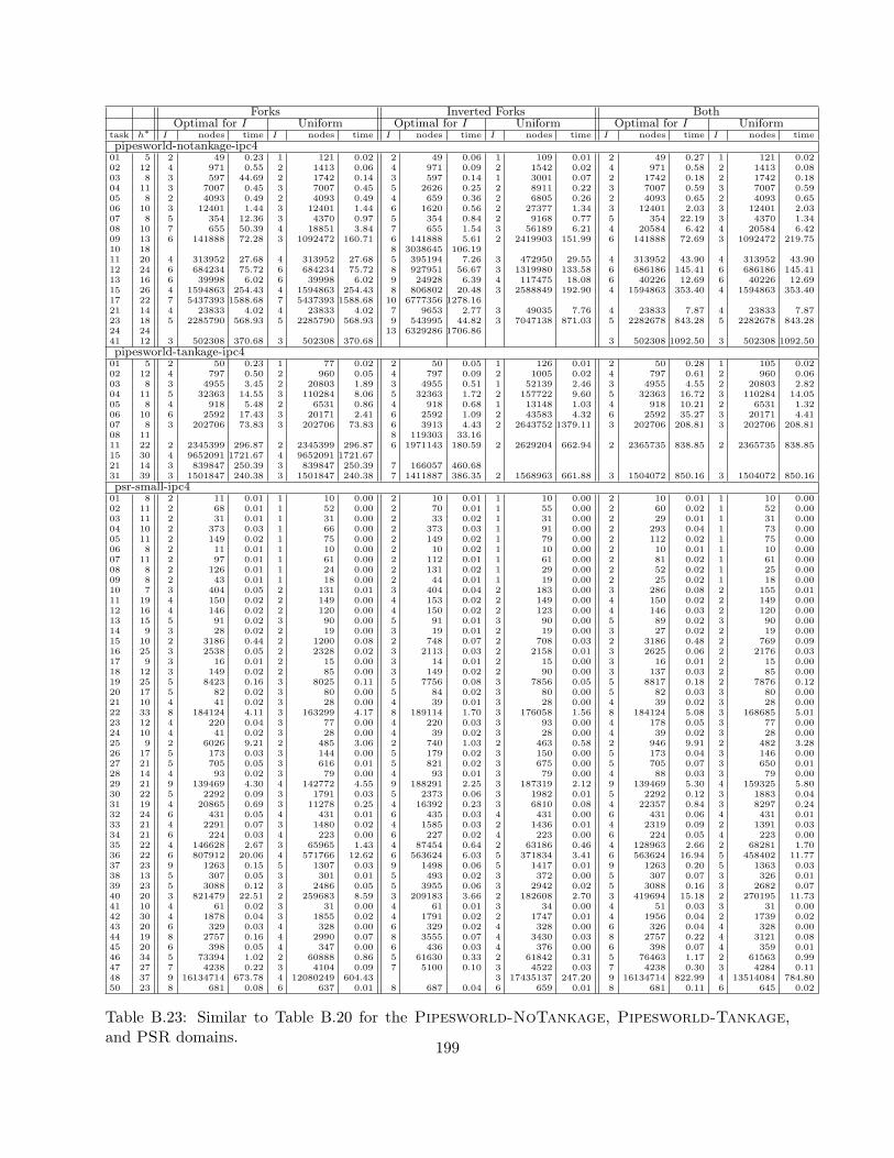
Forks Inverted Forks BothOptimal for I Uniform Optimal for I Uniform Optimal for I Uniform
task h∗ I nodes time I nodes time I nodes time I nodes time I nodes time I nodes time
pipesworld-notankage-ipc401 5 2 49 0.23 1 121 0.02 2 49 0.06 1 109 0.01 2 49 0.27 1 121 0.0202 12 4 971 0.55 2 1413 0.06 4 971 0.09 2 1542 0.02 4 971 0.58 2 1413 0.0803 8 3 597 44.69 2 1742 0.14 3 597 0.14 1 3001 0.07 2 1742 0.18 2 1742 0.1804 11 3 7007 0.45 3 7007 0.45 5 2626 0.25 2 8911 0.22 3 7007 0.59 3 7007 0.5905 8 2 4093 0.49 2 4093 0.49 4 659 0.36 2 6805 0.26 2 4093 0.65 2 4093 0.6506 10 3 12401 1.44 3 12401 1.44 6 1620 0.56 2 27377 1.34 3 12401 2.03 3 12401 2.0307 8 5 354 12.36 3 4370 0.97 5 354 0.84 2 9168 0.77 5 354 22.19 3 4370 1.3408 10 7 655 50.39 4 18851 3.84 7 655 1.54 3 56189 6.21 4 20584 6.42 4 20584 6.4209 13 6 141888 72.28 3 1092472 160.71 6 141888 5.61 2 2419903 151.99 6 141888 72.69 3 1092472 219.7510 18 8 3038645 106.1911 20 4 313952 27.68 4 313952 27.68 5 395194 7.26 3 472950 29.55 4 313952 43.90 4 313952 43.9012 24 6 684234 75.72 6 684234 75.72 8 927951 56.67 3 1319980 133.58 6 686186 145.41 6 686186 145.4113 16 6 39998 6.02 6 39998 6.02 9 24928 6.39 4 117475 18.08 6 40226 12.69 6 40226 12.6915 26 4 1594863 254.43 4 1594863 254.43 8 806802 20.48 3 2588849 192.90 4 1594863 353.40 4 1594863 353.4017 22 7 5437393 1588.68 7 5437393 1588.68 10 6777356 1278.1621 14 4 23833 4.02 4 23833 4.02 7 9653 2.77 3 49035 7.76 4 23833 7.87 4 23833 7.8723 18 5 2285790 568.93 5 2285790 568.93 9 543995 44.82 3 7047138 871.03 5 2282678 843.28 5 2282678 843.2824 24 13 6329286 1706.8641 12 3 502308 370.68 3 502308 370.68 3 502308 1092.50 3 502308 1092.50
pipesworld-tankage-ipc401 5 2 50 0.23 1 77 0.02 2 50 0.05 1 126 0.01 2 50 0.28 1 105 0.0202 12 4 797 0.50 2 960 0.05 4 797 0.09 2 1005 0.02 4 797 0.61 2 960 0.0603 8 3 4955 3.45 2 20803 1.89 3 4955 0.51 1 52139 2.46 3 4955 4.55 2 20803 2.8204 11 5 32363 14.55 3 110284 8.06 5 32363 1.72 2 157722 9.60 5 32363 16.72 3 110284 14.0505 8 4 918 5.48 2 6531 0.86 4 918 0.68 1 13148 1.03 4 918 10.21 2 6531 1.3206 10 6 2592 17.43 3 20171 2.41 6 2592 1.09 2 43583 4.32 6 2592 35.27 3 20171 4.4107 8 3 202706 73.83 3 202706 73.83 6 3913 4.43 2 2643752 1379.11 3 202706 208.81 3 202706 208.8108 11 8 119303 33.1611 22 2 2345399 296.87 2 2345399 296.87 6 1971143 180.59 2 2629204 662.94 2 2365735 838.85 2 2365735 838.8515 30 4 9652091 1721.67 4 9652091 1721.6721 14 3 839847 250.39 3 839847 250.39 7 166057 460.6831 39 3 1501847 240.38 3 1501847 240.38 7 1411887 386.35 2 1568963 661.88 3 1504072 850.16 3 1504072 850.16
psr-small-ipc401 8 2 11 0.01 1 10 0.00 2 10 0.01 1 10 0.00 2 10 0.01 1 10 0.0002 11 2 68 0.01 1 52 0.00 2 70 0.01 1 55 0.00 2 60 0.02 1 52 0.0003 11 2 31 0.01 1 31 0.00 2 33 0.02 1 31 0.00 2 29 0.01 1 31 0.0004 10 2 373 0.03 1 66 0.00 2 373 0.03 1 91 0.00 2 293 0.04 1 73 0.0005 11 2 149 0.02 1 75 0.00 2 149 0.02 1 79 0.00 2 112 0.02 1 75 0.0006 8 2 11 0.01 1 10 0.00 2 10 0.02 1 10 0.00 2 10 0.01 1 10 0.0007 11 2 97 0.01 1 61 0.00 2 112 0.01 1 61 0.00 2 81 0.02 1 61 0.0008 8 2 126 0.01 1 24 0.00 2 131 0.02 1 29 0.00 2 52 0.02 1 25 0.0009 8 2 43 0.01 1 18 0.00 2 44 0.01 1 19 0.00 2 25 0.02 1 18 0.0010 7 3 404 0.05 2 131 0.01 3 404 0.04 2 183 0.00 3 286 0.08 2 155 0.0111 19 4 150 0.02 2 149 0.00 4 153 0.02 2 149 0.00 4 150 0.02 2 149 0.0012 16 4 146 0.02 2 120 0.00 4 150 0.02 2 123 0.00 4 146 0.03 2 120 0.0013 15 5 91 0.02 3 90 0.00 5 91 0.01 3 90 0.00 5 89 0.02 3 90 0.0014 9 3 28 0.02 2 19 0.00 3 19 0.01 2 19 0.00 3 27 0.02 2 19 0.0015 10 2 3186 0.44 2 1200 0.08 2 748 0.07 2 708 0.03 2 3186 0.48 2 769 0.0916 25 3 2538 0.05 2 2328 0.02 3 2113 0.03 2 2158 0.01 3 2625 0.06 2 2176 0.0317 9 3 16 0.01 2 15 0.00 3 14 0.01 2 15 0.00 3 16 0.01 2 15 0.0018 12 3 149 0.02 2 85 0.00 3 149 0.02 2 90 0.00 3 137 0.03 2 85 0.0019 25 5 8423 0.16 3 8025 0.11 5 7756 0.08 3 7856 0.05 5 8817 0.18 2 7876 0.1220 17 5 82 0.02 3 80 0.00 5 84 0.02 3 80 0.00 5 82 0.03 3 80 0.0021 10 4 41 0.02 3 28 0.00 4 39 0.01 3 28 0.00 4 39 0.02 3 28 0.0022 33 8 184124 4.11 3 163299 4.17 8 189114 1.70 3 176058 1.56 8 184124 5.08 3 168685 5.0123 12 4 220 0.04 3 77 0.00 4 220 0.03 3 93 0.00 4 178 0.05 3 77 0.0024 10 4 41 0.02 3 28 0.00 4 39 0.02 3 28 0.00 4 39 0.02 3 28 0.0025 9 2 6026 9.21 2 485 3.06 2 740 1.03 2 463 0.58 2 946 9.91 2 482 3.2826 17 5 173 0.03 3 144 0.00 5 179 0.02 3 150 0.00 5 173 0.04 3 146 0.0027 21 5 705 0.05 3 616 0.01 5 821 0.02 3 675 0.00 5 705 0.07 3 650 0.0128 14 4 93 0.02 3 79 0.00 4 93 0.01 3 79 0.00 4 88 0.03 3 79 0.0029 21 9 139469 4.30 4 142772 4.55 9 188291 2.25 3 187319 2.12 9 139469 5.30 4 159325 5.8030 22 5 2292 0.09 3 1791 0.03 5 2373 0.06 3 1982 0.01 5 2292 0.12 3 1883 0.0431 19 4 20865 0.69 3 11278 0.25 4 16392 0.23 3 6810 0.08 4 22357 0.84 3 8297 0.2432 24 6 431 0.05 4 431 0.01 6 435 0.03 4 431 0.00 6 431 0.06 4 431 0.0133 21 4 2291 0.07 3 1480 0.02 4 1585 0.03 2 1436 0.01 4 2319 0.09 2 1391 0.0334 21 6 224 0.03 4 223 0.00 6 227 0.02 4 223 0.00 6 224 0.05 4 223 0.0035 22 4 146628 2.67 3 65965 1.43 4 87454 0.64 2 63186 0.46 4 128963 2.66 2 68281 1.7036 22 6 807912 20.06 4 571766 12.62 6 563624 6.03 5 371834 3.41 6 563624 16.94 5 458402 11.7737 23 9 1263 0.15 5 1307 0.03 9 1498 0.06 5 1417 0.01 9 1263 0.20 5 1363 0.0338 13 5 307 0.05 3 301 0.01 5 493 0.02 3 372 0.00 5 307 0.07 3 326 0.0139 23 5 3088 0.12 3 2486 0.05 5 3955 0.06 3 2942 0.02 5 3088 0.16 3 2682 0.0740 20 3 821479 22.51 2 259683 8.59 3 209183 3.66 2 182608 2.70 3 419694 15.18 2 270195 11.7341 10 4 61 0.02 3 31 0.00 4 61 0.01 3 34 0.00 4 51 0.03 3 31 0.0042 30 4 1878 0.04 3 1855 0.02 4 1791 0.02 2 1747 0.01 4 1956 0.04 2 1739 0.0243 20 6 329 0.03 4 328 0.00 6 329 0.02 4 328 0.00 6 326 0.04 4 328 0.0044 19 8 2757 0.16 4 2990 0.07 8 3555 0.07 4 3430 0.03 8 2757 0.22 4 3121 0.0845 20 6 398 0.05 4 347 0.00 6 436 0.03 4 376 0.00 6 398 0.07 4 359 0.0146 34 5 73394 1.02 2 60888 0.86 5 61630 0.33 2 61842 0.31 5 76463 1.17 2 61563 0.9947 27 7 4238 0.22 3 4104 0.09 7 5100 0.10 3 4522 0.03 7 4238 0.30 3 4284 0.1148 37 9 16134714 673.78 4 12080249 604.43 3 17435137 247.20 9 16134714 822.99 4 13514084 784.8050 23 8 681 0.08 6 637 0.01 8 687 0.04 6 659 0.01 8 681 0.11 6 645 0.02
Table B.23: Similar to Table B.20 for the Pipesworld-NoTankage, Pipesworld-Tankage,and PSR domains.
199
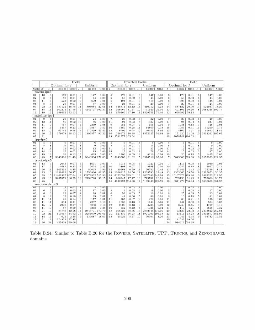
Forks Inverted Forks BothOptimal for I Uniform Optimal for I Uniform Optimal for I Uniform
task h∗ I nodes time I nodes time I nodes time I nodes time I nodes time I nodes time
rovers-ipc501 10 6 173 0.01 6 147 0.00 6 173 0.01 6 147 0.00 6 173 0.01 6 147 0.0002 8 6 50 0.01 6 44 0.00 6 50 0.02 6 44 0.00 6 50 0.02 6 44 0.0003 11 6 523 0.02 5 672 0.01 6 494 0.01 6 419 0.00 6 523 0.02 6 448 0.0104 8 7 20 0.01 6 47 0.00 7 21 0.01 7 20 0.00 7 20 0.01 6 24 0.0005 22 14 587122 18.75 11 808084 22.61 14 518811 12.12 14 410712 9.23 14 587122 20.90 13 522937 18.2907 18 11 602274 37.95 6 4546797 191.34 12 396969 11.57 10 741649 21.01 12 401806 30.56 8 1682245 102.7712 19 12 698692 72.13 12 679360 37.10 11 1529551 76.46 12 698692 79.13
satellite-ipc401 9 7 29 0.01 6 24 0.00 7 29 0.02 6 32 0.00 7 29 0.02 6 29 0.0002 13 11 86 0.02 10 86 0.00 11 91 0.03 8 337 0.00 11 94 0.04 8 241 0.0103 11 9 767 0.07 5 2249 0.08 9 981 0.07 7 656 0.01 9 1038 0.13 7 728 0.0404 17 16 1457 0.23 10 9817 0.57 16 1380 0.28 11 14860 0.38 16 1085 0.41 11 11250 0.7605 15 10 63761 9.98 7 279569 49.47 13 6906 0.98 10 46453 4.92 13 4169 1.67 9 61692 18.8506 20 15 378078 38.13 10 1496577 92.22 16 228672 10.38 10 1572327 51.68 16 171620 21.08 10 1518261 105.6507 21 18 2511377 265.04 18 2078741 686.02
tpp-ipc501 5 5 6 0.01 5 6 0.00 5 6 0.01 4 6 0.00 5 6 0.01 5 6 0.0002 8 8 9 0.01 8 9 0.00 8 9 0.01 7 11 0.00 8 9 0.01 8 9 0.0003 11 11 12 0.02 11 12 0.00 11 12 0.01 9 27 0.00 11 12 0.02 10 16 0.0004 14 14 15 0.02 14 15 0.00 14 15 0.02 11 78 0.00 14 15 0.02 13 47 0.0005 19 19 20 0.12 15 623 0.02 17 1306 0.05 13 5110 0.08 19 20 0.13 15 1455 0.0506 25 7 5843306 201.49 7 5843306 179.03 7 5843306 81.32 5 6916518 95.86 7 5843306 215.08 6 6153923 222.35
trucks-ipc501 13 7 2043 0.07 5 1691 0.03 7 1013 0.05 6 1027 0.01 7 1117 0.08 6 1039 0.0302 17 9 11681 0.33 7 9624 0.23 10 2898 0.07 9 2898 0.04 10 2942 0.18 8 2957 0.1103 20 11 105292 4.45 8 80693 2.99 12 19568 0.59 11 20752 0.44 12 21443 1.42 10 22236 1.1404 23 13 1699483 56.87 8 1753866 48.55 13 1036115 24.56 11 1205793 23.48 13 1363663 59.56 9 1315672 50.3505 25 15 11461967 607.64 9 12472562 515.50 15 6172038 225.61 13 8007189 242.98 15 10107973 599.86 10 9483222 512.5507 23 13 3237871 166.29 10 2134728 96.15 14 626947 17.47 13 719751 16.91 14 763790 61.29 11 755608 50.7208 25 16 4012227 204.98 14 5199440 221.76 16 6341279 786.44 13 6630689 687.95
zenotravel-ipc301 1 1 2 0.03 1 2 0.00 1 2 0.03 1 2 0.00 1 2 0.05 1 2 0.0002 6 5 9 0.03 4 17 0.00 5 9 0.03 3 18 0.00 5 9 0.05 4 17 0.0003 6 6 83 0.07 4 28 0.01 6 53 0.03 5 18 0.01 6 25 0.09 5 12 0.0104 8 8 12 0.10 5 99 0.01 7 44 0.06 5 88 0.01 8 10 0.15 5 81 0.0105 11 11 20 0.14 8 177 0.01 11 105 0.07 9 220 0.01 11 88 0.21 9 136 0.0206 11 11 634 0.21 8 2287 0.10 11 1830 0.13 9 1144 0.05 11 444 0.30 9 504 0.0507 15 12 2979 0.27 8 5088 0.16 12 2806 0.13 9 4234 0.09 12 3240 0.45 9 4199 0.1908 11 10 57 0.99 7 3268 0.35 10 632 0.42 8 1026 0.12 11 119 1.71 8 1655 0.3209 21 19 84749 12.58 14 2844771 177.70 18 966627 68.56 15 2842546 176.05 20 73137 22.02 15 2433822 262.8410 22 21 110557 34.92 17 2283679 295.65 21 527430 56.23 18 1921903 196.38 22 13316 13.23 18 1832871 383.9911 14 13 621 2.35 9 139687 18.63 13 45924 5.47 10 76904 8.20 13 1046 4.45 9 93782 19.5112 21 19 374833 127.85 20 111037 69.6613 26 24 425408 229.06 24 984912 714.39
Table B.24: Similar to Table B.20 for the Rovers, Satellite, TPP, Trucks, and Zenotraveldomains.
200
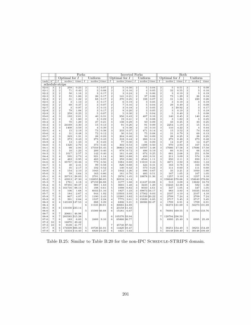
Forks Inverted Forks BothOptimal for I Uniform Optimal for I Uniform Optimal for I Uniform
task h∗ I nodes time I nodes time I nodes time I nodes time I nodes time I nodes time
schedule-strips02-0 3 2 259 0.23 2 5 0.07 2 5 0.30 2 5 0.04 2 5 0.51 2 5 0.0802-1 2 2 71 0.40 2 3 0.08 2 3 0.16 2 4 0.05 2 32 0.55 2 3 0.1002-2 2 2 50 1.16 2 3 0.17 2 3 0.24 2 3 0.06 2 3 0.19 2 3 0.1902-3 3 2 55 1.06 2 26 0.17 2 141 0.21 2 37 0.06 2 73 1.29 2 26 0.1802-4 3 2 31 1.22 2 68 0.17 2 370 0.25 2 188 0.07 2 31 1.36 1 220 0.2602-5 2 2 3 1.10 2 3 0.17 2 6 0.19 2 3 0.05 2 3 0.19 2 3 0.1902-6 2 2 68 0.37 2 3 0.07 2 7 0.16 2 5 0.04 2 29 0.49 2 3 0.0902-7 2 2 3 0.97 2 3 0.15 2 3 0.18 2 3 0.05 2 3 39.92 2 3 0.1702-8 2 2 79 1.08 2 3 0.17 2 9 0.20 2 3 0.05 2 3 0.19 2 3 0.1902-9 3 2 259 0.23 2 5 0.07 2 5 0.30 2 5 0.04 2 5 0.49 2 5 0.0803-0 4 3 192 2.01 3 40 0.31 3 956 0.43 2 407 0.16 2 140 0.45 2 140 0.4503-1 2 2 3 1.80 2 3 0.22 2 19 0.41 2 3 0.08 2 3 1.82 2 3 0.2503-2 4 3 70 1.29 3 27 0.21 3 138 0.29 3 50 0.09 3 33 0.25 3 33 0.2503-3 4 3 24169 3.30 3 15 0.13 3 91 0.26 2 91 0.09 3 2254 1.19 3 15 0.1503-4 3 3 1408 3.59 3 4 0.39 3 4 0.38 2 16 0.10 3 110 4.22 3 4 0.4403-5 4 4 15 2.19 3 73 0.38 3 233 0.37 2 471 0.14 4 15 2.52 3 74 0.4303-6 4 4 31 0.48 3 72 0.12 3 30 0.34 2 75 0.08 4 31 0.79 3 69 0.1303-7 4 3 323 1.31 3 28 0.23 3 204 0.40 3 50 0.09 3 28 0.25 3 28 0.2503-8 4 3 273 0.43 3 273 0.43 3 318 0.44 2 266 0.14 3 273 0.48 3 273 0.4803-9 4 3 12 1.33 3 8 0.23 3 77 0.30 3 31 0.09 3 14 0.27 3 14 0.2704-0 5 5 1320 2.70 4 373 0.45 4 302 0.53 3 1498 0.50 5 970 2.93 3 167 0.5404-1 6 5 99 2.94 3 17559 15.45 4 38863 6.93 3 10707 3.48 3 17686 17.58 3 17686 17.5804-2 5 5 10 1.23 4 209 0.40 4 979 0.72 3 406 0.19 4 66 0.34 4 66 0.3404-3 5 5 1017 2.57 3 142 0.40 4 161 0.48 3 674 0.25 5 681 2.68 3 251 0.5804-4 5 4 595 2.73 4 921 1.14 4 965 0.88 3 450 0.31 4 211 3.09 3 574 1.3904-5 6 4 483 0.95 4 483 0.95 4 259 0.66 3 4544 1.11 3 850 2.11 3 850 2.1104-6 6 5 35757 10.46 4 779 0.56 4 1084 0.69 3 11610 2.44 5 4671 2.92 3 1834 1.4304-7 5 4 40 2.41 3 99 0.58 4 826 0.68 3 424 0.31 3 163 0.78 3 163 0.7804-8 5 5 35 2.17 3 102 0.52 4 140 0.42 3 573 0.24 3 111 0.60 3 111 0.6004-9 4 4 154 2.10 2 1043 1.27 3 1942 1.26 2 996 0.67 4 35 2.21 2 1050 1.6605-0 5 5 59 3.64 3 163 0.86 4 161 0.76 3 483 0.51 3 167 1.05 3 167 1.0505-1 6 6 20713 28.03 5 2701 2.95 5 2976 1.45 3 18878 11.36 4 1257 3.10 4 1257 3.1005-2 7 5 43913 47.30 4 118855 86.65 5 30518 6.14 3 158640 178.66 3 158640 178.6605-3 7 6 1761 4.18 4 27159 24.88 5 3177 1.68 3 41447 13.08 6 513 3.09 4 13622 16.7205-4 6 5 97355 60.37 4 989 1.63 5 3665 1.48 4 3433 1.29 5 13243 12.38 4 582 1.3605-5 6 5 161716 88.15 5 198 0.61 5 1098 0.82 3 9550 4.61 4 347 1.05 4 347 1.0505-6 7 6 106 1.68 4 6033 11.16 5 1827 1.23 3 49873 16.17 6 983 3.92 4 10325 16.6305-7 6 5 184 2.67 4 944 1.92 5 13503 3.93 3 17562 9.03 4 2107 4.10 4 2107 4.1005-8 7 6 867 4.07 5 1190 2.43 5 12285 3.82 3 61539 20.22 4 2709 7.24 4 2709 7.2405-9 6 5 391 2.84 4 1537 2.24 4 7775 3.61 3 15829 6.85 3 2717 5.45 3 2717 5.4506-2 6 4 143169 147.53 4 888 3.29 4 6206 5.21 3 26986 22.47 4 1709 6.91 4 1709 6.9106-4 8 6 11535 20.81 6 30065 14.89 5 56273 131.69 5 56273 131.6906-5 8 6 131030 233.14 6 23158 11.4306-6 8 5 15589 46.68 6 15181 6.67 6 76091 169.55 5 41764 133.7606-7 9 7 20661 46.9806-8 8 7 203585 315.38 6 105570 33.94 7 120794 236.5007-0 7 6 183 6.03 5 2489 9.10 6 65866 36.77 5 6995 25.49 5 6995 25.4907-2 10 9 16870 49.4207-3 10 9 9139 41.77 7 45740 37.5607-7 8 6 174509 306.33 5 10726 41.01 6 14420 10.47 5 38251 154.49 5 38251 154.4907-9 8 7 53334 114.40 6 6829 19.20 6 4421 5.62 5 30148 109.49 5 30148 109.49
Table B.25: Similar to Table B.20 for the non-IPC Schedule-STRIPS domain.
201