Implementation of Automated 3D Defect Detection for LowSignal-to Noise Features in NDE Data

R. Grandin and J. Gray

Center for NDE, Iowa State University, 1915 Scholl Road, Ames, IA 50011 USA

Abstract. The need for robust defect detection in NDE applications requires the identification of subtle, low-contrast changesin measurement signals usually in very noisy data. Most algorithms rarely perform at the level of a human inspector andoften, as data sets are now routinely 10+ Gigabytes, require laborious manual inspection. We present two automated defectsegmentation methods, simple threshold and a binomial hypothesis test, and compare effectiveness of these approaches innoisy data with signal to noise ratios at 1:1. The defect-detection ability of our algorithm will be demonstrated on a 3DCT volume, UT C-scan data, magnetic particle images, and using simulated data generated by XRSIM. The latter is aphysics-based forward model useful in demonstrating the effectiveness of data processing approaches in a simulation whichincludes complex defect geometry and realistic measurement. These large data sets represent significant demands on computeresources and easily overwhelm typical PC platforms; however, the emergence of graphics processing units(GPU) processingpower provides a means to overcome this bottleneck. Processing large, multi-dimensional datasets requires an optimal GPUimplementation which addresses both computational complexity and memory-bandwidth usage.

Keywords: Automated Image Segmentation, Low Signal-to-Noise, Low Contrast, GPU ComputingPACS: 07.05.Pj, 81.70.-q, 81.70.Tx, 87.57.cj, 87.57.cm

INTRODUCTION

The NDE community is faced with the growing problem of “big data”. Optical images are typically several megabyteseach, while computed tomography (CT) and phased-array ultrasonics routinely require 10+ gigabytes. Separate fromthe need to simply store this data, efficient analysis methods are required to extract relevant, useful information from“mountains of data”. Our ability to collect data is out-stripping our ability to segment the data and reliably identifyfeatures. These data quantities will only continue to grow as time moves forward [1]. The problem facing the NDEcommunity is to automate reviews of larger datasets with low signal to noise ratio (SNR) properties with the capabilityof a human inspector.

Unfortunately, most computer algorithms are unable to match the data segmentation ability of a human inspectorand algorithms processing gigabytes of data are often too slow for industrial applications. The low SNR property ofNDE data can be seen in figures 1 and 2, where the SNR’s are 0.84:1 and 0.18:1 respectively. In figure 1 the simpleflaw is easily seen with the human eye, but difficult to accurately size when looking at the line-trace. A threshold whichrejects false-calls will severely under-size the flaw. In figure 2 the flaw is made thinner, thus dramatically reducing itscontrast. It is still visible to the eye, but the line trace shows no indication of the flaw.

FIGURE 1. Low-contrast flaw easy to see with the eye, but difficult to accurately identify computationally. Image is simulatedfilm radiograph of ellipsoidal void within a casting, radiograph generated by XRSIM. SNR = 0.84:1.

FIGURE 2. Low-contrast flaw difficult to see with the eye, but nearly-impossible to accurately identify computationally. Imageis simulated film radiograph of ellipsoidal void within a casting, radiograph generated by XRSIM. SNR = 0.18:1.

In this paper we will demonstrate the performance of an automated algorithm which is shown to be capable ofreliably identifying subtle, low-contrast flaws in a variety of NDE datasets.

TECHNICAL APPROACH

The algorithm used is based upon a statistical analysis of spatial and amplitde distributions rather than a simplecomparison of point values. Such an approach is predicated on the presence of stationary statistics. Stationary statisticsrequires that the mean and variance of our data remains constant throughout the dataset. In-general, this is not the case.However, by identifying and removing any underlying long length-scale trends we can achieve a constant mean. Letus first consider the removal of long length-scale trends, and then the statistical analysis itself.

Trend Identification and Removal

Trends within NDE datasets arise from a number of sources, for example, part geometry, systematic trends inequipment, and analysis assumptions, all of which can introduce long length-scale trends in data. A common trend inCT reconstruction is beam hardening - a trend resulting from the assumption that the incident beam is mono-energetic,a situation that does not typically happen. The result is a bowl-shaped or shell structure, seen in the left side of figure3. The variation results from the low energy photons in the white x-ray spectrum being absorbed more-heavily at theouter surface.

Trend-identification can be accomplished using a number of filter types, with the median filter being simple andeffective. Median filters do well at smoothing point noise while maintaining edges. They become burdensome withlarger images and filter templates requiring large bandwidth between the computer processor and memory when sortingvalues. The available bandwidth is rapidly saturated, especially with today’s multi-core processors, causing the filterperformance to be capped by a low-performance ceiling.

Many CPU performance ceilings can be mitigated through the application of GPU-computing. GPU computing usesthe hundreds of processor cores on a graphics processing unit (GPU) to perform calculations in a massively-parallelmanner. A GPU will still suffer from the memory bandwidth limitations we observe on a CPU and an alternate tomedian filtering must be considered if we are to maximize performance.

An alternate algorithm, called Bilateral Filtering, was introduced in 1998 [2]. The bilateral filter calculates aweighted average of values within its kernel, with weights determined both by the spatial proximity of the points to thecentral pixel and by the similarity of pixel values. This consideration of pixel intensities allows the filter to preserveedges and reject outlier values. The weighted average typically uses a Gaussian distribution, but any functional formmay be chosen.

The bilateral filter can be described by equations 1 and 2, where I0 is a reference intensity value, I j is the intensityof the jth element of the kernel, d j is the distance of the jth element to the reference value’s location, σD controls thedistance (domain) weighting, σR controls the intensity (range) weighting, and I′ is the post-filter intensity value.

w j = e− 1

2

((I j−I0)

2

σ2R

+d2

jσ2

D

)(1)

FIGURE 3. Example of beam-hardening trend in CT reconstruction slice (left). Same slice with trend removed is shown on theright. Small intensities are represented by white. The trend-removal algorithm is unoptimized and still under development. Thesmooth line on the left is to guide the eye and is offset from the data for clarity to separate it from the actual trend in the data.

I′ =∑w jI j

∑w j(2)

The additional calculations involved with the Gaussian weighting make this filter well-suited for implementation ona GPU due to the massively-parallel architecture. Performing bilateral filtering on a 1920 x 1400 image, with an 11 x11 kernel requires 35 seconds on a serial CPU, 4.5 seconds on a parallel CPU with 8 parallel threads, and 0.21 secondson a GPU. The use of the GPU becomes more advantageous as the images and kernels grow. X-ray detectors and CTvolumes can easily span 4000+ pixels in each dimension, and kernels of 100 elements or more may be required toadequately capture the long length-scale trends.

Once the trend is identified, it is removed from the data using simple subtraction. After subtraction we are left withdata of constant mean background value and a constant noise variance. Any regions which have local means and/orvariances different from these background values can then reliably be considered defects.

Statistical Analysis

After achieving stationary noise statistics by removing background trends, we can then identify defects through astatistical analysis of distributions [3]. Figure 4 shows the same flattened CT slice from figure 3 with two areas ofintrest marked. A reference area is identified, and encloses a region containing only background noise. It is this noisewhich must have stationary statistics throughout the dataset.

A smaller test region is also marked. This region will be swept through the dataset, and for each position in thedataset the defect-detection analysis will be performed by comparing the shapes of the dashed-line and solid-linedistributions. For the slice shown on the left of figure 4, the corresponding distributions are shown on the right of thesame figure.

When viewing the histograms on the right side of figure 4 we can see a distinct difference between the twodistributions. We see that the test region has a distribution which is broader and shorter than that of the referencedistribution. And upon closer inspection we can also see that the test distribution is also left-skewed while the referencedistribution appears symmetric.

The basic idea in this test is to observe that the noise is described by a distribution. A Gaussian distribution withmean µ and standard deviation σ describes an ensemble of actual noise distributions in an image. Most of the valuesare clustered around the mean, as seen in the solid-line histogram in figure 4. Any of the ensemble of observed noise

FIGURE 4. Example distributions from flattened data. Reference area is larger box (left) and corresponds to the solid line in thehistogram (right). The test area is the smaller box and dashed line.

distributions following this description will have a similar shape, maximum height, and standard deviation. However,the noise distribution of a pore, the dashed line, is clearly different from the noise distribution shown by the solid line.The statistical question is: what is the likelihood that the dashed-line distribution is an instance of the ensemble ofnoise patterns described by the solid-line histogram?

To give an example, if 50 tosses of a fair coin are recorded we would expect to have 25 heads and 25 tails. If thesetosses are repeated 1000 times, we will see a distribution which is centered on 25 heads and has some variance whichindicates that observing 23 or 24 heads is relatively common, but observing only 1 or 2 is very uncommon. If welet the distribution of these 1000 trials represent the expected distribution of a fair coin, we can then use a secondcoin of unknown fairness and repeat the process. Using a zeta test we can determine if the distribution observedfrom the unknown coin significantly deviates from that of the fair coin. Similarly, we can use a zeta test to evaluatethe probability of the dashed-line histogram in figure 4 being an instance of the noise distribution described by thesolid-line distribution.

This is a robust analysis method that will be shown in the following section to work well with low-contrast noisy datafrom several different NDE inspections. Further, the dimensionality of the data used to generate the distributions doesnot affect the statistical analysis. The following examples are based on 2D images, but collapsing to 1D or expandingto 3D will not adversely affect the analysis. This statistical analysis has not been implemented on a GPU yet, but isreadily executed in parallel on a multi-core CPU.

APPLICATION TO NDE DATA

X-Ray CT

Given the immense quantity of data generated by a CT inspection and reconstruction, let us first consider such adataset. For this example we scanned a dolomite rock core with our high-resolution CT system. Using a microfocustube to exploit geometric magnification we performed the reconstruction on a grid of 450 slices, with each slicecontaining 1000 x 1000 pixels. The entire dataset required 2 gigabytes of memory.

Figure 5 shows a slice from this reconstruction. This slice contains several features-of-interest including large-scaleporosity, micro-porosity, and line-type indications from a fracture face which intersects the reconstruction plane.

The right image in figure 5 shows many small indications, which may appear to be spurious results. However, if wezoom-in on the upper-right corner of the slice to show detail we can see that the small indications actually correspondnicely with small-scale porosity (figure 6). These small-scale porosity indications have SNR’s below 1:1.

In addition to considering individual CT slices, individual slice results can be stacked to provide a volumetricanalysis. By considering the entire volume we can perform detailed studies on flaw morphology and connectivity

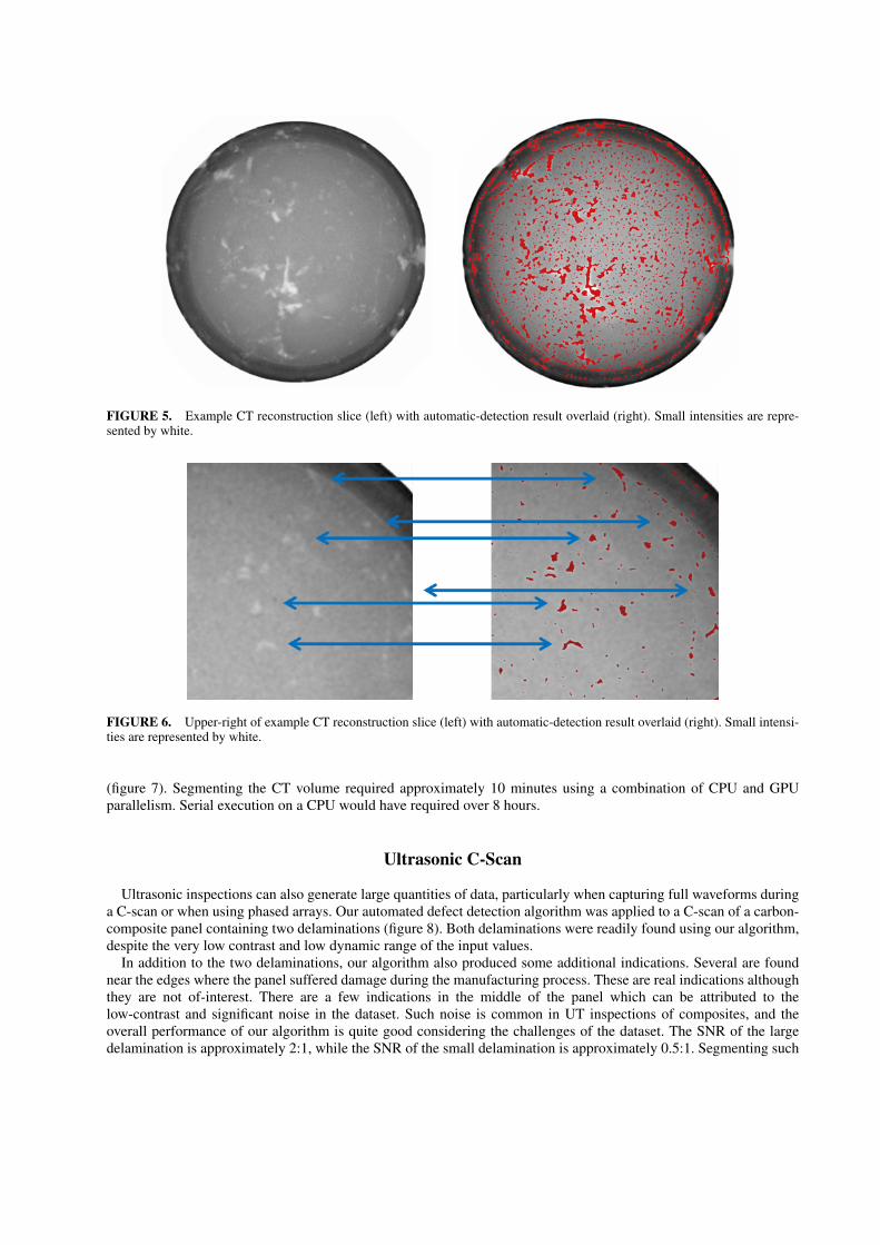
FIGURE 5. Example CT reconstruction slice (left) with automatic-detection result overlaid (right). Small intensities are repre-sented by white.

FIGURE 6. Upper-right of example CT reconstruction slice (left) with automatic-detection result overlaid (right). Small intensi-ties are represented by white.

(figure 7). Segmenting the CT volume required approximately 10 minutes using a combination of CPU and GPUparallelism. Serial execution on a CPU would have required over 8 hours.

Ultrasonic C-Scan

Ultrasonic inspections can also generate large quantities of data, particularly when capturing full waveforms duringa C-scan or when using phased arrays. Our automated defect detection algorithm was applied to a C-scan of a carbon-composite panel containing two delaminations (figure 8). Both delaminations were readily found using our algorithm,despite the very low contrast and low dynamic range of the input values.

In addition to the two delaminations, our algorithm also produced some additional indications. Several are foundnear the edges where the panel suffered damage during the manufacturing process. These are real indications althoughthey are not of-interest. There are a few indications in the middle of the panel which can be attributed to thelow-contrast and significant noise in the dataset. Such noise is common in UT inspections of composites, and theoverall performance of our algorithm is quite good considering the challenges of the dataset. The SNR of the largedelamination is approximately 2:1, while the SNR of the small delamination is approximately 0.5:1. Segmenting such

FIGURE 7. Detail flaw morphology (left) and connectivity (right) extracted from volumetric analysis.

FIGURE 8. UT C-scan (left) and automated-detection result (right) for scan of 1“ and 1/2” delaminations in a carbon-compositepanel.

a small image (150 x 200 pixels) only required 1 minute on a serial CPU, but this could be reduced to 3 seconds usinga combination of CPU and GPU parallelism.

Magnetic Particle Inspection

As a final example of applicability to NDE data, let us consider a photograph of a visual inspection. Figure 9 shows atool used to verify proper performance of the fluid bath in a magnetic particle inspection (MPI). Typically an operatorwill look at the ring as it is shown in the picture and then make a determination if the cracks are properly visible.This is a very subjective process and efforts to bring objectivity and consistency to this analysis have met with greatdifficulty due to the noise caused by particles captured in surface roughness and variable lighting conditions.

Although the cracks appear to be easily visible in figure 9, we see in figure 10 that a simple threshold cannotadequately capture the crack details. However, in the right image of figure 10 we can see a significant improvementin detection. This dramatic improvement was obtained using a typical photograph (8 bits per RGB channel), and evenbetter performance is expected when using images with greater bit-depth due to the improved signal resolution. SNRvaries from approximately 3:1 for the large, wide cracks to less than 0.5:1 for the small, thin cracks. Segmenting this1500 x 1500 image required 2 minutes on a serial CPU, which was reduced to 5 seconds using a combination of CPUand GPU parallelism.

Similar to what is observed in the CT slice results, what may appear to be errant indications in figure 10 are actuallyseen to be valid defect indications when we zoom-in on the lower-right corner of the images of the figure, as seen in

FIGURE 9. Photograph of grinding cracks used for MPI bath qualification tests. The diagonal line in the photo marks the lineover which intensity values are plotted adjacent to the photo. The horizontal line in the plot shows the threshold used in the leftimage of figure 10. Notice the inability to capture low-contrast peaks without including significant noise.

FIGURE 10. Result of applying a simple threshold (left) and our automated detection algorithm (right) to the photograph infigure 10.

figure 11. We see in figure 11 that many of the smaller cracks are now at least partially marked.

CONCLUSIONS

We have shown a successful implementation of a multi-dimensional image segmentation algorithm suitable for largeNDE datasets. The performance of this algorithm has been demonstrated using several varied datasets containinglow-contrast and low dynamic-range data, and in each case our algorithm performed very well. The algorithmconsistently identified the correct features while avoiding both false-calls and missed defects. While not yet matchingthe segmentation performance of a human inspector, the implementation of this algorithm is a significant step towardsthat goal.

While achieving this analytical performance, the recent quantum leap in computing power was leveraged to allowthese results to be obtained in minutes rather than hours or days as would have been required only a short time ago.Use of GPU computing allowed us to reduce the time required to de-trend the data by two orders of magnitude, fromthe tens of minutes to a few seconds.

FIGURE 11. Detail of lower-right corner of images in figure 10, showing simple threshold result (left) and our automateddetection result (right).

FUTURE WORK

Building upon the results shown here, we will extend the analysis to be truly three-dimensional. The addition ofan additional dimension will increase the computational load by an order of magnitude and require implementingthe statistical analysis algorithm on the GPU architecture. We will also work to appropriately correct for the footprint-effect which occurs from discretely-stepping a finite-sized test window across the data and to improve the performancewith complex materials.

A logical extension of this work is to automatically characterize the flaws which are detected. Such characterizationcould include size distributions, position analysis, and study of flaw morphology. Further, characterization results canbe used in the development of matched filters which can be efficiently used to search through a dataset for specifictypes of flaws.

Finally, a defect-detection algorithm such as this can be used to develop objective, robust figures of merit whichmay be used to evaluate the effectiveness of data-processing algorithms. Quantitative NDE simulation tools may becoupled with this defect-detection algorithm to develop figures of merit which objectively evaluate the quality andsensitivity of the inspection.

ACKNOWLEDGMENTS

This material is based on work supported by the Army Research Laboratory as part of cooperative agreementnumber W911NF0820036 at the Center for Nondestructive Evaluation at Iowa State University. Magnetic particleand ultrasonic sample data provided courtesy Dan Barnard, Brady Engle, Darrel Enyart, and Ajith Subramanian.

REFERENCES

1. J. Gray, “Nondestrucive Evaluation Needs for Today and the Future,” in CNDE 25th Anniversary, 2011.2. C. Tomasi, and R. Manduchi, “Bilateral Filtering for Gray and Color Images,” Proceedings of the IEEE International Conference

on Computer Vision, Bombay, India, 1998.3. J. Gray, J. Zhang, , and I. Gray, “Application of NDE Simulation to Estimate Probability of Detection,” in QNDE 2004, 2004.4. N. Sheikh, Medium resolution computed tomography through phosphor screen detector and 3D image analysis, Master’s thesis,

Iowa State University (2006).