Combustion and Flame 158 (2011) 2199–2213

Contents lists available at ScienceDirect

Combustion and Flame

journal homepage: www.elsevier .com/locate /combustflame

Implementation of a dynamic thickened flame model for large eddy simulationsof turbulent premixed combustion

G. Wang, M. Boileau, D. Veynante ⇑Laboratoire EM2C – CNRS, Ecole Centrale Paris, Châtenay Malabry, France

a r t i c l e i n f o a b s t r a c t

Article history:Received 3 August 2010Received in revised form 1 April 2011Accepted 4 April 2011Available online 27 April 2011

Keywords:Turbulent premixed combustionLarge eddy simulationDynamic model

0010-2180/$ - see front matter � 2011 The Combustdoi:10.1016/j.combustflame.2011.04.008

⇑ Corresponding author. Fax: +33 1 47 02 80 35.E-mail address: denis.veynante@em2c.ecp.fr (D. V

A dynamic version of the thickened flame model for large eddy simulations (TFLES) of turbulent premixedcombustion is implemented by coupling two independent codes through MPI (Message Passing Interface)running on massively parallel machines. The combustion code, AVBP, solves the usual filtered Navier–Stokes, mass fractions and energy balance equations on unstructured meshes while a second code takesadvantage of the knowledge of resolved flow structures to automatically adjust the combustion modelparameter from filtered resolved flow fields. This approach is tested against data from the F1, F2 andF3 pilot stabilised jet-flames experimentally investigated by Chen and coworkers. The model parametersdetermined dynamically are quite different for these cases, evidencing the decisive advantage of thedynamic procedure while statistical results are in good agreement with experimental data. The extra costinduced by the dynamic model is here about 20% but further optimisation remains possible.

� 2011 The Combustion Institute. Published by Elsevier Inc. All rights reserved.

1. Introduction

Large eddy simulation (LES) is an attractive and now widely-used tool to describe turbulent premixed combustion [1,2]. Be-cause the largest turbulent motions are explicitly computed whileonly the effects of the smallest ones are modelled, the overall mod-el contribution is reduced compared to RANS (Reynolds AveragedNavier–Stokes equations) and this LES technique gives access tounsteady flame behaviours as encountered during transient igni-tion [3], combustion instabilities [4–6] or cycle-to-cycle variationsin internal combustion engines [7,8]. However, a primary recurrentproblem lies in the flame thickness which is typically too thin to beresolved on the LES grid size. Different strategies have been devel-oped to manage this issue. The level-set (G-equation) approachconsists in tracking the flame front solving a propagation equation[2,4,9,10] but, as providing information only on the flame front po-sition and not on its structure, the coupling with the flow equa-tions remains challenging [11]. Another solution is to artificiallythicken the flame front (Thickened Flame model for LES, TFLES)[3,5,6,12,13] or to introduce a filter larger than the mesh size to re-solve the filtered flame structure [14,15].

Another challenge is to model the unresolved flame/turbulenceinteractions whether in terms of subgrid scale turbulent flamespeed, for example when using the level-set formalism [2], flamesurface density [7,14,16] or flame surface wrinkling factor[12,13,17]. Most of the models proposed in the literature more or

ion Institute. Published by Elsevier

eynante).

less assume an equilibrium between turbulence motions and flamesurface and are expressed in terms of algebraic expressions butcannot handle transient situations [7]. Some propose to solve a bal-ance equation [7,16,17] but relatively few attempts have beenmade to develop dynamic combustion models [1,2,10,18]. The ba-sic idea of such models, first developed to describe subgrid scalemomentum transport [19], is to take advantage of the knowninstantaneous resolved large scales to automatically adjust themodel parameters, determined by comparing the application ofthe model to the LES resolved field (filter scale) and to this resolvedfield once filtered by a second filter (test-filter scale). Unfortu-nately, momentum transport and combustion phenomena behavecompletely differently. Most of the turbulence energy lies in re-solved scale motions and the subgrid scale energy represents onlya small part of the total energy, a way to check the LES quality [20].On the other hand, combustion is mainly a subgrid scale phenom-enon and looking for a linear parameter may lead to an ill-posedproblem [18]. This difficulty may be overcome by looking for amodel exponent [18] or for a related quantity such as the subgridscale turbulent flame speed [10].

Dynamic modelling is primarily based on the filtering of theinstantaneous resolved fields at a test filter scale, larger than theoriginal LES filter [1]. The model is then assumed to hold at bothscales with the same model parameter leading to a ‘‘Germano-like’’relation providing this parameter. The present work is based on adynamic version of the TFLES model [18], which gives an automaticscheme to recast the subfilter flame wrinkling lost due to thicken-ing. The validation by Charlette et al. [18] is only limited to a verysimple academic case of a statistically one-dimensional premixed

Inc. All rights reserved.

2200 G. Wang et al. / Combustion and Flame 158 (2011) 2199–2213

flame propagating in a time-decaying isotropic turbulent flowusing an LES version of the direct numerical simulation (DNS) codeNTMIX [21,22]. LES results were compared to DNS data for low tur-bulence levels (a posteriori tests) and against turbulent flame speedmeasurements for large Reynolds numbers. No attempt has beenmade yet to simulate more practical and complex situations, lead-ing to new challenges. For example, when running on massivelyparallel machines a code working with unstructured meshes, acomputationally efficient (in terms of CPU time and memoryrequirements) test filter operation is not obvious, especially whenthis filter should be sufficiently large to contain some wrinkling ofthe resolved flame front. The approach retained here is to run adedicated filtering code coupled to the main flow field solver andexchanging data at given time intervals, as already proposed tocompute turbulent combusting flows including radiative heattransfer [23]. Another difficulty is the prediction at both filterand test filter scales of the turbulence intensity entering the flamefront wrinkling model. A more robust dynamic determination ofmodel parameter is then proposed assuming implicitly that the in-ner cutoff scale does not depend on the local turbulence intensity.

The model details are described in Section 2 while its practicalimplementation is presented in Section 3. The jet flame configura-tion investigated experimentally by Chen et al. [24] is described to-gether with computational details in Section 4. This experimenthas been already simulated with a dynamic model for the turbu-lent burning velocity by Knudsen and Pitsch [10]. Numerical re-sults are presented and discussed in Section 5. The ability of thedynamic model to respond to changes in operating conditions isalso analysed.

2. Modelling

2.1. The Thickened Flame model (TFLES)

A correct laminar premixed flame propagation on a coarse gridmay be achieved by artificially thickening the flame front, solvingthe balance equations for species mass fractions Yk:

@qYk

@tþr � ðquYkÞ ¼ �r � ðqFVkYkÞ þ

_xkðQÞF

ð1Þ

where q is the density, u the velocity vector, Vk the diffusion veloc-ity of species k, expressed here using the Hirschfelder and Curtissapproximation [1,25], and _xk the reaction rate of species k, esti-mated, for example, from Arrhenius laws or chemical tables. Q de-notes any quantity entering the computation of the reaction rate,such as species mass fractions or temperature. As the molecular dif-fusion and chemical source terms have been multiplied and dividedby the thickening factor F, respectively, the thickened flame frontpropagates at the same laminar flame speed S0

L as the original flameof thickness d0

L but its thickness becomes Fd0L [26]. For sufficiently

large values of F, the flame structure can be resolved on a coarsegrid. In LES, Eq. (1) is recast as [1,12]:

@�qeY k

@tþr � ð�q~ueY kÞ ¼ r � ðFNDqVk

eY kÞ þND

F_xkðeQ Þ ð2Þ

where Q and eQ denotes filtered and mass-weighted filtered quanti-ties, respectively, ð�qeQ ¼ qQÞ. The subgrid scale wrinkling factor ND

measures the ratio of the total flame surface to the resolved flamesurface in the filter volume and is then linked to the subgrid scaleflame surface lost because of the thickening process. Eq. (2) propa-gates a flame front of thickness Fd0

L at the turbulent flame speedST ¼ NDS0

L (in practice, the loss of the subgrid scale flame surfaceis compensated by a higher flame speed). Charlette et al. [13] modelthe wrinkling factor with a power-law relationship on the ratio ofouter (D) to inner (gc) cutoff scale, as:

ND ¼ 1þ Dgc

� �b

ð3Þ

This expression is similar to fractal models writing ND ¼ ðD=gcÞDf�2,

where Df is the fractal dimension of the flame surface [27,28] but:(i) Charlette et al. [13] add unity to the scale ratio D/gc to ensurethat ND tends toward unity when gc� D, i.e. when the flame frontis not wrinkled at the subgrid scale level; (ii) b is not expected to bea universal parameter and could depend on scales D, gc and otherrelevant parameters such as Reynolds number or turbulence inten-sity. Assuming that each relevant turbulence motion acts indepen-dently on the flame front and integrating their action estimatedfrom DNS over a homogeneous and isotropic turbulence spectrumgives the Charlette et al. model [13]:

ND ¼ 1þminD

d0L

� 1;CDD

d0L

;u0DS0

L

;ReD

!u0DS0

L

" # !b

ð4Þ

where the efficiency function CD takes into account the net strain-ing effect of all relevant turbulent scales smaller than D and is pro-vided in Appendix A. ReD is the subgrid scale Reynolds number andb a model parameter to be specified. Note that we have replacedD=d0

L by D=d0L � 1

� �in the original expression to maximise the wrin-

kling factor ND by the fractal model, i.e. NmaxD ¼ D=d0

L

� �b[27,28]. In

fact, Charlette et al. [13] implicitly supposed that D=d0L � 1 when

deriving their model, an assumption not always satisfied for the finegrid meshes available today. Eq. (4) implicitly supposes that D P d0

L

and predicts a wrinkling factor lying between unity (ND = 1) whensubgrid scale turbulence vanishes ðu0D ¼ 0Þ and Nmax

D ¼ D=d0L

� �b.

An automatic determination of the b parameter during the com-putation, is now proposed.

2.2. Dynamic formulation

The reaction rate _xk entering Eq. (2) is recast as [18]:

�_xk ¼ND

F_xkðeQ Þ ¼ ND

Dd0

L_xkðeQ Þ ¼ ND

DWD;kðeQ Þ ð5Þ

introducing the function WD;kðeQ Þ. The flame thickening factor Fmeasures the ratio of the resolved flame thickness, correspondingto a filter size, and the laminar flame thickness: F ¼ D=d0

L . A test fil-ter of size cD (c P 1) is then introduced and noted �z}|{, the corre-sponding mass-weighted filter being denoted bQ , so thatqz}|{ bQ ¼ qQ

z}|{. A Germano-like identity is obtained by equalling

the test-filtered resolved reaction rate to the reaction rate estimatedat the test-filter level when both are averaged over a given domain(h�i operator), meaning that the total reaction rate over this domainshould be the same when estimated from the resolved LES field orfrom the test-filtered field. This averaging is introduced to avoidunphysical behaviours (‘‘weak form’’, see [18]): as Eq. (4) is basedon flame wrinkling arguments, the averaging volume should con-tain some wrinkling of the test-filtered flame front. Then:

�_xk

z}|{¼ ND

DWD;kðeQ Þzfflfflfflfflfflfflfflffl}|fflfflfflfflfflfflfflffl{* +

¼ NcD

cDWcD;k

beQ� �� �ð6Þ

Assuming that the parameter u0D, given by Eq. (4), is uncorrelatedfrom the local values of WDð~qÞ over the averaging volume gives:

b ¼log chWD;kðeQ Þzfflfflfflfflffl}|fflfflfflfflffl{

i=hWcD;kðbeQ Þi !

log1þmin cD=d0

L � 1;CcDhu0cDi=S0L

1þmin D=d0

L � 1;CDhu0Di=S0L

0@ 1A ð7Þ

One of the practical difficulties in the implementation of thisdynamic identity proposed by Charlette et al. [18] is the correct

G. Wang et al. / Combustion and Flame 158 (2011) 2199–2213 2201

estimation of the turbulence intensity at both filter u0D� �� �

and test-filter u0cD

D E scales from the known resolved fields. A simple linear

relation based on homogeneous and isotropic turbulence theory,u0cD ¼ c1=3u0D, as well as the expression proposed by Colin et al.[12] (see Eq. 12 in Section 3.2 below) were first tested but foundto make the dynamic procedure numerically unstable because ofmodelling uncertainties. To avoid the determination of both turbu-lence intensities u0D

� �and u0cD

D E; b is determined in a first step sim-

plifying Eq. (7) in the limiting case of large turbulence intensities,when the maximum value of the wrinkling factor is given by thefractal model:

limu0

D!1

ND ¼D

d0L

!b

; limu0cD!1

NcD ¼cDd0

L

!b

ð8Þ

leading to:

b ¼ 1þ logðhWD;kðeQ Þzfflfflfflfflffl}|fflfflfflfflffl{i=hWcD;kð

beQ ÞiÞlogðcÞ ð9Þ

This last expression corresponds to estimating the exponent b fromthe maximum possible value of the wrinkling factor according toEq. (4) or to assume that the inner cutoff scale gc in Eq. (3) doesnot depend on the turbulence intensity u0D. Of course, once b isdetermined from Eq. (9), the wrinkling factor ND is estimated fromEq. (4) where the subgrid scale turbulence intensity, u0D, enters. Thewrinkling factor then evolves in the range 1 6 ND 6 D=d0

L

� �b. The

estimation of u0cD is now no longer required.The practical implementation of the dynamic model is now

described.

3. Practical implementation

3.1. Principle

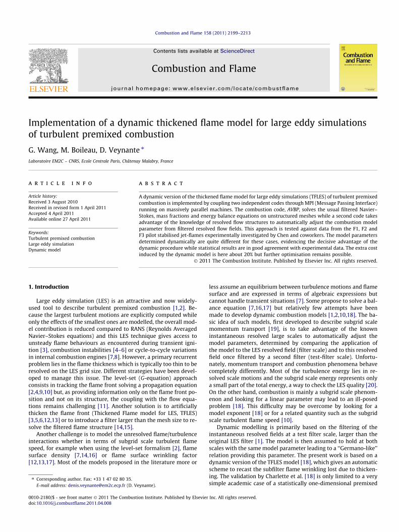
The proposed implementation, designed to run on massivelyparallel machines using unstructured meshes, is based on the cou-pling of two codes through MPI (Message Passing Interface), asshown in Fig. 1. The test filtering and the determination of themodel parameter b (Eq. 9) is done by a dedicated solver, called FIL-TER (for FILTERing operation), outside the main combustion codeAVBP that solves the Navier–Stokes and mass species balance equa-tions [29]. The AVBP code provides instantaneous filtered temper-ature, species mass fractions and reaction rate fields to the filteringcode. This last code then determines and returns to AVBP the bparameter that may be local (i.e. depending on the local positionin the flow field) or global (a single b value for the entire flow field),an option adapted to homogenous flows to reduce computationalcosts and data exchanges, but evolves with time.

Fig. 1. Coupling between two Fortran codes dedicated to turbulent combustion(AVBP) and test filtering (FILTER). Each code runs according to its own time step andexchange data from time to time through MPI.

This approach is very flexible and versatile [23]: the structure ofeach code is not affected by the coupling procedure. Combustionand filtering codes can then be developed independently. Note thatone large-size test filter may require data from several processorsof AVBP solver. Another advantage lies in the fact that physical timescales to be considered are quite different. As AVBP explicitly solvescompressible Navier–Stokes equations, its time step DtLES is lim-ited by the propagation speed of acoustic waves (Courant–Fried-rich–Levy criterion, based on the local sound speed). On theother hand, parameters of dynamic models are more likely relatedto the evolution of the flow turbulence motions and expected toevolve according to a convective time DtConv. As subsonic flowsare considered here, this time is larger than the acoustic time DtLES

by one or two orders of magnitude. Then the model parametersonly need to be updated at time steps DtConv = nDtLES with n largerthan unity.

An asynchronous strategy is followed here. The two codes worksimultaneously and independently until they exchange data everyDtConv physical time step (Fig. 1) through MPI. A correct load bal-ancing (i.e. a similar charge of every processor used) is achievedby adjusting the number of processors devoted to each code so thatthe combustion code performs n iterations while FILTER deter-mines a complete b field (see Section 3.4). In practice, the resolvedflow field at time t updates b at time t + DtConv but this approxima-tion is found to have no influence on the final results when DtConv

(or iteration number n) is kept sufficiently small, as shown inSection 5.5.

As a first step, we will look in the following for a uniform b va-lue over the entire reacting flow field, depending only on time.Then, the averaging volume denoted h�i in Eq. (9) will be the entirecomputational domain, containing here all the flame. Three rea-sons motivated this choice: (i) the practical implementation is eas-ier and related computational costs reduced; (ii) to look for a localb value requires to specify the averaging volume h�iwhich becomesan additional parameter to be investigated; (iii) results could be di-rectly compared with non-dynamic constant b value cases. How-ever, preliminary tests show that the dynamic procedure workswhen looking for local b values. Note that some recent develop-ments of dynamic models for the unresolved momentum transportalso look for a unique model parameter [30,31], a procedure foundmore suitable for complex flows where no homogenous directionsare available to average the model parameter and avoid numericalinstabilities. However, to look for a unique parameter is possible inthis last case with the Vreman turbulence model [32] which is ableto predict vanishing subgrid scale momentum transport for fullyresolved laminar flows, whatever the value of the model parameteris, but would not be a relevant with the usual Smagorinsky model[33] which requires a zero model parameter in laminar flow re-gions. The situation is similar here for combustion: Eq. (4) correctlypredicted unity flame surface wrinkling factors when local subgridscale turbulence vanishes (i.e. u0D tends towards zero) whatever theglobal b value is.

3.2. Turbulence and combustion modelling

A single step, irreversible chemistry is considered here for themethane oxidation:

CH4 þ 2O2 ! CO2 þ 2H2O; ð10Þ

The fuel reaction rate is modelled by an Arrhenius law:

_xCH4 ¼ A � qYCH4

MCH4

� �nCH4 qYO2

MO2

� �nO2

exp � Ea

RT

� �ð11Þ

where T; YCH4 ;YO2 ;MCH4 ;MO2 and R denote temperature, fuel andoxygen mass fractions, corresponding molar weights and the

2202 G. Wang et al. / Combustion and Flame 158 (2011) 2199–2213

perfect gas constant, respectively. The pre-exponential factor, theactivation energy and the model exponents are A = 1.1 � 1010 (cgs),Ea = 20,000 cal/mol, nCH4 ¼ 1:0 and nO2 ¼ 0:5 [29]. These values leadto a laminar flame speed S0

L ¼ 0:40 m/s and a burnt gas adiabatic tem-perature Tb = 2328 K in atmospheric stoichiometric conditions.

Three thickening factors (set equal to F = 4, 6 and 8) of the TFLESmodel are tested on three grids of different resolution. The dynam-ically thickened flame (DTF) model [29,34,35] is adopted to modu-late the thickening factor from the maximum value F inside thereaction zone to unity away from flame front according to a sensorbased on the chemical reaction rate. The DTF model has beendeveloped to avoid the artificial enhancement of molecular diffu-sion outside the reaction zone when reactants are not perfecly pre-mixed (see Refs. [34,35] for details). Note that the expression‘‘dynamically thickened flame model’’ introduced by Légier et al.[34,35] is confusing. In this method, the thickening factor of theTFLES is locally adjusted as a function of the reaction rate to avoidthe modification of the diffusive transport outside the reactionzone but the DTF model is not dynamic in the usual LES sensewhere the effects of subgrid scales are modelled adjusting modelparameters on the fly from the known resolved scales.

The subscale turbulence intensity u0D at scale D entering thewrinkling factor ND (Eq. 4) is estimated as [12,29]:

u0D ¼D

nxDx

� �1=3

u0nxDx¼ c2D

3x jr2ðr � euÞj D

nxDx

� �1=3

ð12Þ

where Dx denotes the mesh size, estimated from the local cell vol-ume, c2 = 2 and nx = 10. The length factor D/nxDx corrects the Colinet al. expression [12] designed to estimate the turbulent intensityu0nxDx

corresponding to scales below nxDx [29]. Note that Eq. (12) isdesigned to cancel out the contribution of thermal expansion,which is not related to turbulence, when estimating u0D. A filteredSmagorinsky model [36] is retained to describe unresolved momen-tum and species transport. We focus here on the development, testand implementation of a dynamic combustion model and, as a firststep, a non-dynamic model is considered for turbulent momentumtransport. A dynamic Smagorinsky model [19,37] will be easilyimplemented in FILTER in the future.

3.3. Test filtering

A Gaussian test filter is used here and defined as:

GðxÞ ¼ 6

pbD2

� �3=2

exp � 6bD2ðx2

1 þ x22 þ x2

3Þ �

ð13Þ

where bD is the test-filter size and x(x1,x2,x3) the spatial coordinatesrelative to the filtered node position. Contrary to usual 3 or 5 pointsfilters [38,39], widely used and discussed in LES, the test filter forthe dynamic flame model must be sufficiently large to contain wrin-kling of the resolved flame front. Note also that the filter size is spec-ified here in terms of physical coordinates and is independent of thelocal mesh size. Accordingly, the dynamic procedure is expected to benot affected by local mesh refinements. For each node i in the unstruc-tured mesh, the test-filtered quantities are calculated from filteredquantities /j at nodes j by a discrete convolution operator as:

/i

z}|{¼Xj2Di

/j � Vj �wi;j=Xj2Di

Vj �wi;j ð14Þ

where Vj denotes the cell volume linked to the j node, Di the filtercutoff domain, wi,j the Gaussian weight of node j to i given by Eq.(13). In practice, wi,j is interpolated from a one-dimensional tablesets prior to computation. The filter cut-off domain Di should atleast include all the nodes j within a distance from the node ishorter than the test filter size bD. For each node, the test-filterprocedure then involves tens of thousands neighbouring nodes

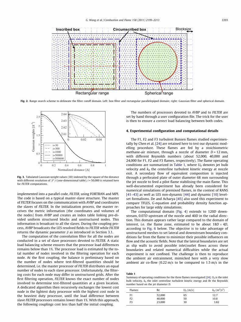
due to the required bD size. As the computer memory is not suffi-cient to prestore such information for all the domain nodes, the do-main search and filtering algorithms are performed for eachdetermination of test-filtered fields.

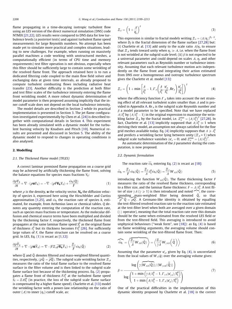
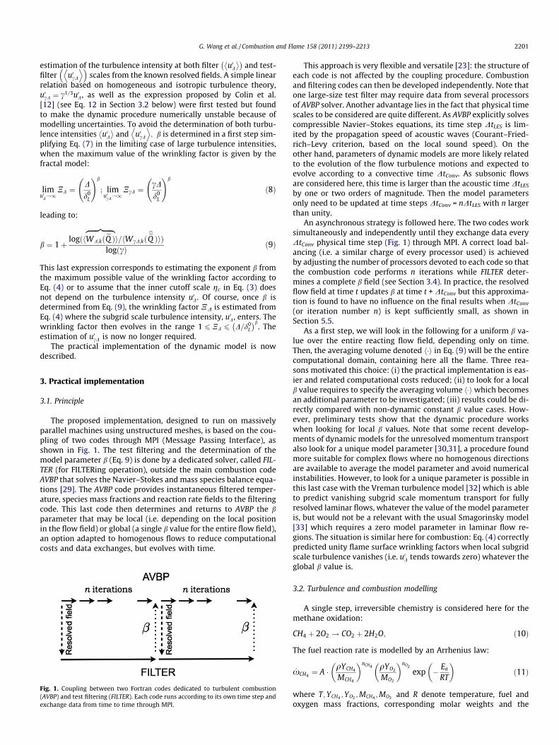
An efficient range search algorithm named cells [40] is adopted todelineate the filter cutoff domain. As shown in Fig. 2, the unstructuredmesh is initially divided into several uniform structured blocks,which are indexed with 3D identifiers according to their positionsin physical space. All the unstructured nodes are linked to differentblocks through their coordinates. The block size is set to several timesthe mesh size. Then, for a spherical range search for the cutoff domainof Gaussian filter, the distance computation and comparison are lim-ited to the circumscribed box, shown in right part of Fig. 2. Also aGaussian weight (wi,j) table, displayed in Fig. 3 and indexed by thesquare of the distance, is precomputed to avoid the repetition ofexpensive floating-point calculations of Eq. (13). According to this ap-proach, the filtering domain information (Di, Vj�wi,j and

Pj2Di

Vj �wi;j)for one node i is temporally stored in a common buffer (lower than 5MBytes). Once the convolution operation (Eq. 14) is performed todetermine the five required test-filtered quantities (density, fueland oxidizer mass fractions, temperature, reaction rate) at node i,the buffer is recycled to repeat the procedure for the next nodei + 1. The cost of the determination of the Gaussian kernel is aboutthree times the convolution operation costs and could be saved whensufficiently large memories will be available in the future.

The rectangular range search algorithm displayed in the left partof Fig. 2 corresponds to the potential use of a box filter (local averag-ing operation). The weight of each node in box filter is independentof distance, i.e. wi,j always equals unity in Eq. 14, and the only infor-mation required is the filter cutoff domain. Then, the first step is lim-ited to the determination of the inscribed and circumscribed boxesfor the search range. The box filtering costs about one-fifth of theGaussian filtering cost and is thus attractive. However, two reasonsmotivated the choice of a Gaussian filter for this work: (i) the largeeddy simulations of infinitely thin flame front implicitly requireGaussian LES filters (see [14]) and to use test Gaussian filters seemsmore relevant; (ii) box filters may suffer from numerical uncertain-ties due to combination of their discrete form, especially on unstruc-tured meshes, with sharp cut-off edges (in Gaussian filters, points inthe vicinity of edges are weighted by very low wi,j values).

A key point when filtering a LES flow field is to estimate the cor-responding effective filter size, i.e. the c value that should enter theGermano-like identity (Eq. 6), ensuring a correct physical behav-

iour for planar laminar flame (i.e. chWD;kðeQ Þzfflfflfflfflffl}|fflfflfflfflffl{i ¼ hWcD;kð

beQ Þi when

ND = NcD = 1). Combining two Gaussian filters of size D and bD,respectively, gives:

c ¼ 1þbDD

!224 351=2

ð15Þ

Unfortunately, to thicken a flame in TFLES is not strictly equivalentto filtering a flame front following the standard LES definitions. Anequivalent laminar flame thickness in terms of Gaussian LES filter,dl, is then introduced to write D = Fdl. Its value is calibrated fromone-dimensional steady premixed laminar flame and set todl � 2:2d0

L , where d0L is the laminar flame thickness defined from

the temperature profile gradient. Tests (not displayed here) show

that Eq. (15) correctly gives chWD;kð eQ Þzfflfflfflfflffl}|fflfflfflfflffl{i ¼ hWcD;kð

beQ Þi for planar

laminar flames whatever F and bD values are.

3.4. Code FILTER and coupling with AVBP

The large-size Gaussian test filter operator and the determina-tion of the b parameter of the combustion model (Eq. 9) are

Rectangular range Spherical range

BlocksizeCircumscribed boxInscribed box

Fig. 2. Range search scheme to delineate the filter cutoff domain. Left: box filter and rectangular parallelepiped domain; right: Gaussian filter and spherical domain.

0.60 0.2 0.4 0.8 1

Normalized distance [Δ]

0

0.5

1

1.5

2

2.5

Gau

ssia

n w

eigh

ts [

Δ-3]

i=30i=300i=1000i=50000i=500000

0 0.02 0.04

2.61

2.62

2.63

2.64

Fig. 3. Tabulated Gaussian weight values (3D) indexed by the square of the distancewith different resolution of bD2=i (one-dimensional table). i = 50,000 is retained herefor FILTER computations.

Table 1Summary of operating conditions for the three flames investigated [24]. U0 is the inletbulk velocity, k0 the inlet centreline turbulent kinetic energy and Re the Reynoldsnumber based on the jet diameter D.

Flames Re U0 (m/s) k0 (m2/s2)

F1 52,000 65 12.7F2 40,000 50 10.8F3 23,000 30 3.82

G. Wang et al. / Combustion and Flame 158 (2011) 2199–2213 2203

implemented into a parallel code, FILTER, using FORTRAN and MPI.The code is based on a typical master-slave structure. The masterof FILTER focuses on the communication with AVBP and coordinatesthe slaves of FILTER. In the initialization process, the master re-ceives the metric information (the coordinates and volumes ofthe nodes) from AVBP and creates an index table linking pre-di-vided uniform structured blocks and unstructured nodes. Thisinformation is broadcast to all the slaves. During the coupling pro-cess, AVBP broadcasts the LES resolved fields to FILTER while FILTERreturns the dynamic parameter b as introduced in Section 3.1.

The computation of the convolution filter for all the nodes areconducted in a set of slave processors devoted to FILTER. A staticload balancing scheme ensures that the processor load differencesremains below than 1%. The processor load is estimated by the to-tal number of nodes involved in the filtering operation for eachnode. At the first coupling, the balance is preliminary based onthe number of nodes where test-filtered quantities should bedetermined, i.e. the master processor of FILTER distributes an equalnumber of nodes to each slave processor. Unfortunately, the filter-ing costs for each node may differ in unstructured grids. After thefirst filtering operation, FILTER knows the exact number of nodesinvolved to determine test-filtered quantities at a given location.A dedicated algorithm then recursively exchanges the lowest costnode in the lightest duty processor with the highest cost node inthe heaviest duty processor, until the load difference betweenslave FILTER processors remains lower than 1%. With this approach,the following couplings cost less than half the initial coupling.

The numbers of processors devoted to AVBP and to FILTER areset by hand through a user configuration file. The trick for the useris then to ensure a correct load balancing between both codes.

4. Experimental configuration and computational details

The F1, F2 and F3 turbulent Bunsen flames studied experimen-tally by Chen et al. [24] are retained here to test our dynamic mod-elling procedure. These flames are fed by a stoichiometricmethane-air mixture, through a nozzle of diameter D = 12 mm,with different Reynolds numbers (about 52,000, 40,000 and24,000 for F1, F2 and F3 flames, respectively). The flame operatingconditions are summarized in Table 1, where U0 denotes jet bulkvelocity and k0 the centerline turbulent kinetic energy at nozzleexit. A secondary flow of equivalent composition is injectedthrough a perforated plate of outer diameter 68 mm surroundingthe jet nozzle to feed a pilot flame stabilising the main flame. Thiswell-documented experiment has already been considered fornumerical simulations of premixed flames, in the context of RANS[41–43] as well as LES non-dynamic [44] and dynamic [10] level-set formalisms. De and Acharya [45] also used this experiment tocompare TFLES, G-equation and probability density function ap-proaches for large eddy simulations.

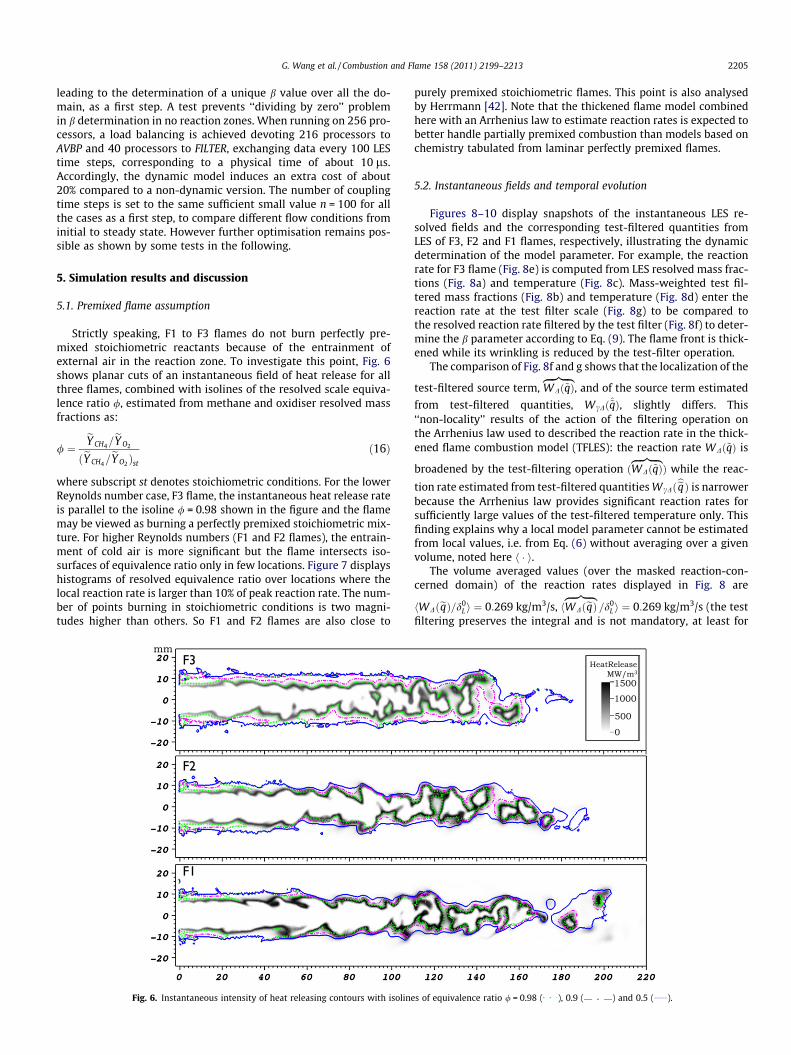
The computational domain (Fig. 4) extends to 120D down-stream, 0.07D upstream of the nozzle and 40D in the radial direc-tion. This domain appears rather large compared to the domain ofinterest, i.e. the flame zone, estimated to be about 18D � 4D,according to Fig. 6 below. The objective is to take advantage ofunstructured meshes to set lateral and downstream boundary con-ditions far from the flame to minimize their possible influences onflow and the acoustic fields. Note that the lateral boundaries are setas slip walls to avoid possible inlet/outlet flows across theseboundaries and related numerical difficulties while the actualexperiment is not confined. The challenge is then to reproducethe ambient air entrainment, mimicked here with a very slowambient air co-flow (0.22 m/s to be compared to 1.5 m/s in the

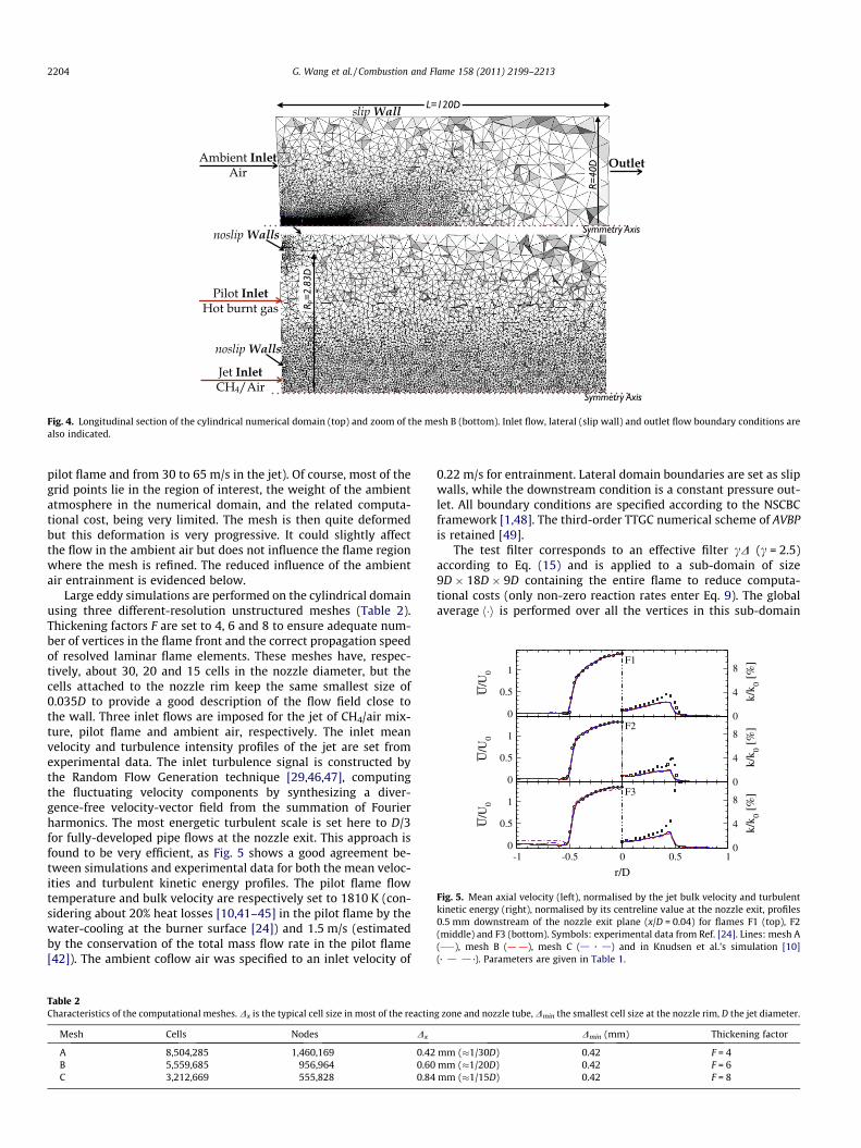
Fig. 4. Longitudinal section of the cylindrical numerical domain (top) and zoom of the mesh B (bottom). Inlet flow, lateral (slip wall) and outlet flow boundary conditions arealso indicated.

r/D

0

0.5

1

U/U

0

0

0.5

1

U/U

0

0

0.5

1

U/U

0

-1 -0.5 0 0.5 10

4

8

k/k 0 [

%]

0

4

8

k/k 0 [

%]

0

4

8

k/k 0 [

%]

F3

F2

F1

Fig. 5. Mean axial velocity (left), normalised by the jet bulk velocity and turbulentkinetic energy (right), normalised by its centreline value at the nozzle exit, profiles0.5 mm downstream of the nozzle exit plane (x/D = 0.04) for flames F1 (top), F2(middle) and F3 (bottom). Symbols: experimental data from Ref. [24]. Lines: mesh A( ), mesh B ( ), mesh C ( ) and in Knudsen et al.’s simulation [10]( ). Parameters are given in Table 1.

2204 G. Wang et al. / Combustion and Flame 158 (2011) 2199–2213

pilot flame and from 30 to 65 m/s in the jet). Of course, most of thegrid points lie in the region of interest, the weight of the ambientatmosphere in the numerical domain, and the related computa-tional cost, being very limited. The mesh is then quite deformedbut this deformation is very progressive. It could slightly affectthe flow in the ambient air but does not influence the flame regionwhere the mesh is refined. The reduced influence of the ambientair entrainment is evidenced below.

Large eddy simulations are performed on the cylindrical domainusing three different-resolution unstructured meshes (Table 2).Thickening factors F are set to 4, 6 and 8 to ensure adequate num-ber of vertices in the flame front and the correct propagation speedof resolved laminar flame elements. These meshes have, respec-tively, about 30, 20 and 15 cells in the nozzle diameter, but thecells attached to the nozzle rim keep the same smallest size of0.035D to provide a good description of the flow field close tothe wall. Three inlet flows are imposed for the jet of CH4/air mix-ture, pilot flame and ambient air, respectively. The inlet meanvelocity and turbulence intensity profiles of the jet are set fromexperimental data. The inlet turbulence signal is constructed bythe Random Flow Generation technique [29,46,47], computingthe fluctuating velocity components by synthesizing a diver-gence-free velocity-vector field from the summation of Fourierharmonics. The most energetic turbulent scale is set here to D/3for fully-developed pipe flows at the nozzle exit. This approach isfound to be very efficient, as Fig. 5 shows a good agreement be-tween simulations and experimental data for both the mean veloc-ities and turbulent kinetic energy profiles. The pilot flame flowtemperature and bulk velocity are respectively set to 1810 K (con-sidering about 20% heat losses [10,41–45] in the pilot flame by thewater-cooling at the burner surface [24]) and 1.5 m/s (estimatedby the conservation of the total mass flow rate in the pilot flame[42]). The ambient coflow air was specified to an inlet velocity of

Table 2Characteristics of the computational meshes. Dx is the typical cell size in most of the reactin

Mesh Cells Nodes Dx

A 8,504,285 1,460,169 0.42B 5,559,685 956,964 0.60C 3,212,669 555,828 0.84

0.22 m/s for entrainment. Lateral domain boundaries are set as slipwalls, while the downstream condition is a constant pressure out-let. All boundary conditions are specified according to the NSCBCframework [1,48]. The third-order TTGC numerical scheme of AVBPis retained [49].

The test filter corresponds to an effective filter cD (c = 2.5)according to Eq. (15) and is applied to a sub-domain of size9D � 18D � 9D containing the entire flame to reduce computa-tional costs (only non-zero reaction rates enter Eq. 9). The globalaverage h�i is performed over all the vertices in this sub-domain

g zone and nozzle tube, Dmin the smallest cell size at the nozzle rim, D the jet diameter.

Dmin (mm) Thickening factor

mm (�1/30D) 0.42 F = 4mm (�1/20D) 0.42 F = 6mm (�1/15D) 0.42 F = 8

G. Wang et al. / Combustion and Flame 158 (2011) 2199–2213 2205

leading to the determination of a unique b value over all the do-main, as a first step. A test prevents ‘‘dividing by zero’’ problemin b determination in no reaction zones. When running on 256 pro-cessors, a load balancing is achieved devoting 216 processors toAVBP and 40 processors to FILTER, exchanging data every 100 LEStime steps, corresponding to a physical time of about 10 ls.Accordingly, the dynamic model induces an extra cost of about20% compared to a non-dynamic version. The number of couplingtime steps is set to the same sufficient small value n = 100 for allthe cases as a first step, to compare different flow conditions frominitial to steady state. However further optimisation remains pos-sible as shown by some tests in the following.

5. Simulation results and discussion

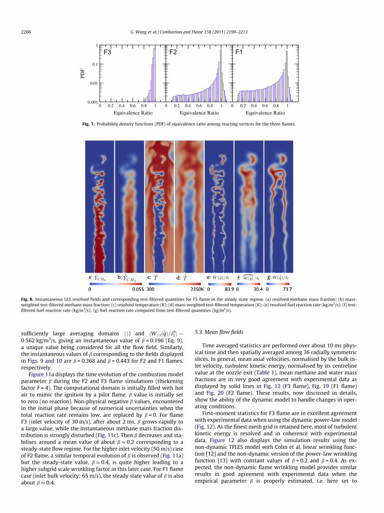
5.1. Premixed flame assumption

Strictly speaking, F1 to F3 flames do not burn perfectly pre-mixed stoichiometric reactants because of the entrainment ofexternal air in the reaction zone. To investigate this point, Fig. 6shows planar cuts of an instantaneous field of heat release for allthree flames, combined with isolines of the resolved scale equiva-lence ratio /, estimated from methane and oxidiser resolved massfractions as:

/ ¼eY CH4=

eY O2

ðeY CH4=eY O2 Þst

ð16Þ

where subscript st denotes stoichiometric conditions. For the lowerReynolds number case, F3 flame, the instantaneous heat release rateis parallel to the isoline / = 0.98 shown in the figure and the flamemay be viewed as burning a perfectly premixed stoichiometric mix-ture. For higher Reynolds numbers (F1 and F2 flames), the entrain-ment of cold air is more significant but the flame intersects iso-surfaces of equivalence ratio only in few locations. Figure 7 displayshistograms of resolved equivalence ratio over locations where thelocal reaction rate is larger than 10% of peak reaction rate. The num-ber of points burning in stoichiometric conditions is two magni-tudes higher than others. So F1 and F2 flames are also close to

Fig. 6. Instantaneous intensity of heat releasing contours with isoline

purely premixed stoichiometric flames. This point is also analysedby Herrmann [42]. Note that the thickened flame model combinedhere with an Arrhenius law to estimate reaction rates is expected tobetter handle partially premixed combustion than models based onchemistry tabulated from laminar perfectly premixed flames.

5.2. Instantaneous fields and temporal evolution

Figures 8–10 display snapshots of the instantaneous LES re-solved fields and the corresponding test-filtered quantities fromLES of F3, F2 and F1 flames, respectively, illustrating the dynamicdetermination of the model parameter. For example, the reactionrate for F3 flame (Fig. 8e) is computed from LES resolved mass frac-tions (Fig. 8a) and temperature (Fig. 8c). Mass-weighted test fil-tered mass fractions (Fig. 8b) and temperature (Fig. 8d) enter thereaction rate at the test filter scale (Fig. 8g) to be compared tothe resolved reaction rate filtered by the test filter (Fig. 8f) to deter-mine the b parameter according to Eq. (9). The flame front is thick-ened while its wrinkling is reduced by the test-filter operation.

The comparison of Fig. 8f and g shows that the localization of the

test-filtered source term, WDð~qÞzfflfflffl}|fflfflffl{

, and of the source term estimated

from test-filtered quantities, WcDð~̂qÞ, slightly differs. This‘‘non-locality’’ results of the action of the filtering operation onthe Arrhenius law used to described the reaction rate in the thick-ened flame combustion model (TFLES): the reaction rate WDð~qÞ is

broadened by the test-filtering operation ðWDð~qÞzfflfflffl}|fflfflffl{

Þ while the reac-

tion rate estimated from test-filtered quantities WcDðbeqÞ is narrowerbecause the Arrhenius law provides significant reaction rates forsufficiently large values of the test-filtered temperature only. Thisfinding explains why a local model parameter cannot be estimatedfrom local values, i.e. from Eq. (6) without averaging over a givenvolume, noted here h � i.

The volume averaged values (over the masked reaction-con-cerned domain) of the reaction rates displayed in Fig. 8 are

hWDðeqÞ=d0L i ¼ 0:269 kg/m3/s, hWDðeqÞzfflfflffl}|fflfflffl{

=d0L i ¼ 0:269 kg/m3/s (the test

filtering preserves the integral and is not mandatory, at least for

s of equivalence ratio / = 0.98 ( ), 0.9 ( ) and 0.5 ( ).

0.6

Equivalence Ratio

0.001

0.01

0.1

1

PDF

0.6

Equivalence Ratio

0.60 0.2 0.4 0.8 1 0 0.2 0.4 0.8 1 0 0.2 0.4 0.8 1

Equivalence Ratio

F3 F2 F1

Fig. 7. Probability density functions (PDF) of equivalence ratio among reacting vertices for the three flames.

Fig. 8. Instantaneous LES resolved fields and corresponding test-filtered quantities for F3 flame in the steady state regime. (a) resolved methane mass fraction; (b) mass-weighted test-filtered methane mass fraction; (c) resolved temperature (K); (d) mass-weighted test-filtered temperature (K); (e) resolved fuel reaction rate (kg/m3/s); (f) test-filtered fuel reaction rate (kg/m3/s); (g) fuel reaction rate computed from test-filtered quantities (kg/m3/s).

2206 G. Wang et al. / Combustion and Flame 158 (2011) 2199–2213

sufficiently large averaging domains h i) and hWcDð~̂qÞ=d0L i ¼

0:562 kg/m3/s, giving an instantaneous value of b = 0.196 (Eq. 9),a unique value being considered for all the flow field. Similarly,the instantaneous values of b corresponding to the fields displayedin Figs. 9 and 10 are b = 0.368 and b = 0.443 for F2 and F1 flames,respectively.

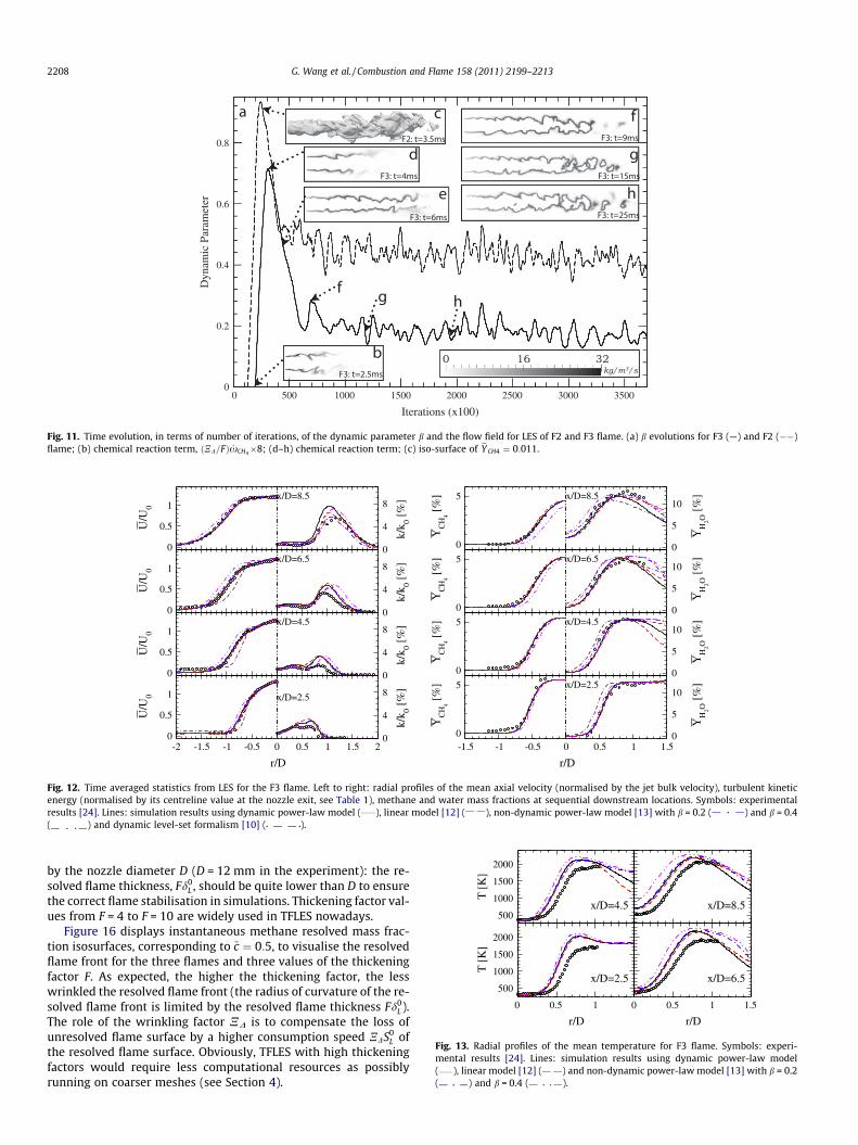
Figure 11a displays the time evolution of the combustion modelparameter b during the F2 and F3 flame simulations (thickeningfactor F = 4). The computational domain is initially filled with hotair to mimic the ignition by a pilot flame. b value is initially setto zero (no reaction). Non-physical negative b values, encounteredin the initial phase because of numerical uncertainties when thetotal reaction rate remains low, are replaced by b = 0. For flameF3 (inlet velocity of 30 m/s), after about 2 ms, b grows rapidly toa large value, while the instantaneous methane mass fraction dis-tribution is strongly disturbed (Fig. 11c). Then b decreases and sta-bilises around a mean value of about b � 0.2 corresponding to asteady-state flow regime. For the higher inlet velocity (50 m/s) caseof F2 flame, a similar temporal evolution of b is observed (Fig. 11a)but the steady-state value, b � 0.4, is quite higher leading to ahigher subgrid scale wrinkling factor in this later case. For F1 flamecase (inlet bulk velocity: 65 m/s), the steady state value of b is alsoabout b � 0.4.

5.3. Mean flow fields

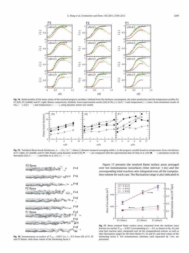
Time averaged statistics are performed over about 10 ms phys-ical time and then spatially averaged among 36 radially symmetricslices. In general, mean axial velocities, normalised by the bulk in-let velocity, turbulent kinetic energy, normalised by its centrelinevalue at the nozzle exit (Table 1), mean methane and water massfractions are in very good agreement with experimental data asdisplayed by solid lines in Fig. 12 (F3 flame), Fig. 19 (F1 flame)and Fig. 20 (F2 flame). These results, now discussed in details,show the ability of the dynamic model to handle changes in oper-ating conditions.

First-moment statistics for F3 flame are in excellent agreementwith experimental data when using the dynamic power-law model(Fig. 12). As the finest mesh grid is retained here, most of turbulentkinetic energy is resolved and in coherence with experimentaldata. Figure 12 also displays the simulation results using thenon-dynamic TFLES model with Colin et al. linear wrinkling func-tion [12] and the non-dynamic version of the power-law wrinklingfunction [13] with constant values of b = 0.2 and b = 0.4. As ex-pected, the non-dynamic flame wrinkling model provides similarresults in good agreement with experimental data when theempirical parameter b is properly estimated, i.e. here set to

Fig. 9. Instantaneous LES resolved fields and corresponding test-filtered quantitiesfor F2 flame in the steady state regime. (a) resolved fuel reaction rate; (b) test-filtered fuel reaction rate; (c) fuel reaction rate computed from test-filteredquantities. Units: kg/m3/s.

Fig. 10. Instantaneous LES resolved fields and corresponding test-filtered quantitiesfor F1 flame in the steady state regime. (a) resolved fuel reaction rate; (b) test-filtered fuel reaction rate; (c) fuel reaction rate computed from test-filteredquantities. Units: kg/m3/s.

G. Wang et al. / Combustion and Flame 158 (2011) 2199–2213 2207

b = 0.2, the steady state value reached by the dynamic procedure.In contrast, using b = 0.4, the value adapted to case F2, leads tounsatisfactory results for F3 flame (Fig. 12). A similar conclusionis reached when using b = 0.2 for the non-dynamic modelling ofF2 flame (Fig. 20). These results demonstrate the interest of the dy-namic formalism even if looking for a unique parameter value forall the computational domain: b is automatically determined with-out requiring a case by case hand made adjustment depending onoperating conditions. Figure 12 also displays recent results byKnudsen and Pitsch [10] using a dynamic level set formalism. Theiragreement with experimental data appears to be less satisfactory.

Figure 13 shows that the mean temperature is overestimated byabout 200 K in numerical simulations compared to experimentalvalues. Similar behaviours are also observed for Flames F1 andF2. To investigate this point, both experimental and numericalmean temperature and mean methane (CH4) and water (H2O) massfractions are converted into mean progress variables according to:

~c ¼eQ � Q u

Q b � Q uð17Þ

where Qu and Qb correspond to the fresh and burnt gas values of thequantity Q considered, respectively. Tb = 2248 K was used in com-puting the progress variable from experimental mean temperatureprofiles by Chen et al. [24] and Tb = 2328 K for the simulation cases.The burnt gas values of mass fractions are set to Yb

CH4¼ 0 and

YbH2O ¼ 0:124, both for experimental and simulation data. Mean pro-

gress variables are displayed in Fig. 14 for the three flames F1, F2

and F3. The overestimation of the mean temperature in numericalresults could be due to the one-step irreversible chemical schemeretained here, neglecting the carbon mono (CO) and dioxide (CO2)chemistry. Radiation heat transfer that may decrease maximumtemperature by about one hundred Kelvin, has also not been takeninto account in simulations. The dilution of the main jet flow by hotgases issued from piloted flames cannot explain such a temperaturedifference as the total mass flux of the piloting flow is only one-fifthto one-tenth of main jet flux. However, the discrepancies betweennumerical results and experimental data might also be due toexperimental uncertainties as mean velocity and mass fractionsprofiles are perfectly captured in simulations, as well as the thermalexpansion due to heat release.

Maximum gradients of mean temperature radial profiles, ex-pressed in terms of turbulent flame brush thickness, dt ¼ ð@½~cT �=@rÞ�1

max, where ½~cT � is the mean resolved progress variable based ontemperature, are also compared to experimental data in Fig. 15(operator [�] denotes temporal averaging). Results are comparableto recent simulations by Herrmann [42] and Kolla et al. [41] andin agreement with experimental data by Chen et al. [24]

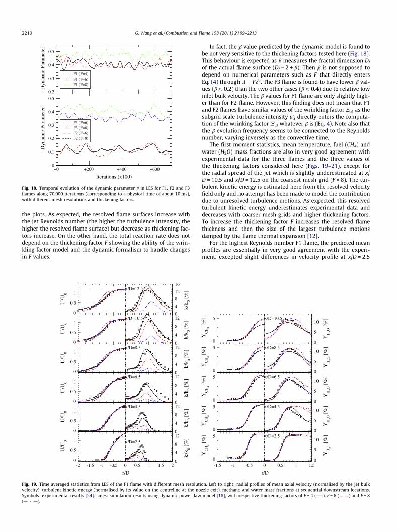
5.4. Influence of the thickening factor and grid meshes

The simulations of the three flames are now conducted on coar-ser mesh grids to investigate the capacity of the dynamic TFLESmodel in handling higher thickening factors, F = 6 and F = 8 (seeTable 2). The practical thickness of the thickened flame, and accord-ingly the maximum value of the thickening factor F is also limited

0 500 1000 1500 2000 2500 3000 3500

Iterations (x100)

0

0.2

0.4

0.6

0.8

Dyn

amic

Par

amet

er

Fig. 11. Time evolution, in terms of number of iterations, of the dynamic parameter b and the flow field for LES of F2 and F3 flame. (a) b evolutions for F3 (—) and F2 (��)flame; (b) chemical reaction term, ðND=FÞ _xCH4�8; (d–h) chemical reaction term; (c) iso-surface of eY CH4 ¼ 0:011.

r/D

0

0.5

1

U/U

0

0

0.5

1

U/U

0

0

0.5

1

U/U

0

0

0.5

1

U/U

0

0

4

8

k/k 0 [

%]

0

4

8

k/k 0 [

%]

0

4

8

k/k 0 [

%]

0

4

8

k/k 0 [

%]

r/D

0

5

10Y

H2O

[%

]

0

5

10

YH

2O [

%]

0

5

10

YH

2O [

%]

0

5

10

YH

2O [

%]

-2 -1.5 -1 -0.5 0 0.5 1 1.5 2 0 0.5 1 1.5-1.5 -1 -0.50

5

YC

H4 [

%]

0

5

YC

H4 [

%]

0

5

YC

H4 [

%]

0

5

YC

H4 [

%]

x/D=2.5

x/D=4.5

x/D=6.5

x/D=8.5

x/D=2.5

x/D=4.5

x/D=6.5

x/D=8.5

Fig. 12. Time averaged statistics from LES for the F3 flame. Left to right: radial profiles of the mean axial velocity (normalised by the jet bulk velocity), turbulent kineticenergy (normalised by its centreline value at the nozzle exit, see Table 1), methane and water mass fractions at sequential downstream locations. Symbols: experimentalresults [24]. Lines: simulation results using dynamic power-law model ( ), linear model [12] ( ), non-dynamic power-law model [13] with b = 0.2 ( ) and b = 0.4( ) and dynamic level-set formalism [10] ( ).

r/D

500

1000

1500

2000

T [

K]

500

1000

1500

2000

T [

K]

0 0.5 1 0 0.5 1 1.5

r/D

x/D=2.5

x/D=4.5

x/D=6.5

x/D=8.5

Fig. 13. Radial profiles of the mean temperature for F3 flame. Symbols: experi-mental results [24]. Lines: simulation results using dynamic power-law model( ), linear model [12] ( ) and non-dynamic power-law model [13] with b = 0.2( ) and b = 0.4 ( ).

2208 G. Wang et al. / Combustion and Flame 158 (2011) 2199–2213

by the nozzle diameter D (D = 12 mm in the experiment): the re-solved flame thickness, Fd0

L , should be quite lower than D to ensurethe correct flame stabilisation in simulations. Thickening factor val-ues from F = 4 to F = 10 are widely used in TFLES nowadays.

Figure 16 displays instantaneous methane resolved mass frac-tion isosurfaces, corresponding to ~c ¼ 0:5, to visualise the resolvedflame front for the three flames and three values of the thickeningfactor F. As expected, the higher the thickening factor, the lesswrinkled the resolved flame front (the radius of curvature of the re-solved flame front is limited by the resolved flame thickness Fd0

L ).The role of the wrinkling factor ND is to compensate the loss ofunresolved flame surface by a higher consumption speed NDS0

L ofthe resolved flame surface. Obviously, TFLES with high thickeningfactors would require less computational resources as possiblyrunning on coarser meshes (see Section 4).

r/D

0

0.5

1

c [-

]

0

0.5

1

c [-

]

0

0.5

1

c [-

]

0

0.5

1

c [-

]

x/D=2.5

x/D=4.5

x/D=6.5

x/D=8.5

r/D

0

0.5

1

c [-

]

0

0.5

1

c [-

]

0

0.5

1c

[-]

0

0.5

1

c [-

]

x/D=2.5

x/D=4.5

x/D=6.5

x/D=8.5

0 0.5 1 1.50 0.5 1 1.5 0 0.5 1 1.5

r/D

0

0.5

1

c [-

]

0

0.5

1

c [-

]

0

0.5

1

c [-

]

0

0.5

1

c [-

]

x/D=2.5

x/D=4.5

x/D=6.5

x/D=8.5

F3 F2 F1

Fig. 14. Radial profiles of the mean values of the resolved progress variables ~c defined from the methane consumption, the water production and the temperature profiles forF3 (left), F2 (middle) and F1 (right) flames, respectively. Symbols: from experimental results [24] of CH4 ( ), H2O ( ) and temperature ( ). Lines: from simulation results ofCH4 ( ), H2O ( ) and temperature ( ), using dynamic power-law model.

x/D

0

5

10

Flam

e br

ush

thic

knes

s

x/D

2 4 6 8 10 2 4 6 8 10 2 4 6 8 10 12

x/D

(mm) F3 F2 F1

Fig. 15. Turbulent flame-brush thicknesses, dt ¼ ð@½~cT �=@rÞ�1, where [�] denotes temporal averaging while ~cT is the progress variable based on temperature, from calculationsof F1 (right), F2 (middle) and F3 (left) flames using dynamic model [18] ( ) are compared with the experimental data of Chen et al. [24] ( ), simulation results byHerrmann [42] ( ) and Kolla et al. [41] ( ).

Fig. 16. Instantaneous so-surface of eY CH4 ¼ 0:027 (i.e. ~c ¼ 0:5) from LES of F1, F2and F3 flames, with three values of the thickening factor F.

G. Wang et al. / Combustion and Flame 158 (2011) 2199–2213 2209

Figure 17 presents the resolved flame surface areas averagedover ten instantaneous isosurfaces (time interval: 1 ms) and thecorresponding total reaction rates integrated over all the computa-tion volume for each case. The fluctuation range is also indicated in

F3 (30m/s) F2 (50m/s) F1 (65m/s)0

0.01

0.02

Are

a of

iso-

surf

ace

[m2 ]

0

0.1

0.2

0.3

0.4

Inte

gral

rea

ctio

n ra

te [

x10-3

kg/s

]

F=4F=6F=8

Fig. 17. Mean resolved flame surface areas, estimated from the methane massfraction iso-surface eY CH4 ¼ 0:027 (corresponding to ~c ¼ 0:5, as shown in Fig. 16) andtotal fuel reaction rates, integrated over all the computational volume, as well astheir fluctuation ranges for the three flames F1, F2 and F3, and three values of thethickening factor F. Ten instantaneous solutions, each separated by 1 ms, areprocessed.

+0 +200 +400 +600

Iterations (x100)

0

0.1

0.2

0.3

0.4

0.5

Dyn

amic

Par

amet

er

F3 (F=6)F3 (F=8)F2 (F=6)F2 (F=8)

0.2

0.3

0.4

0.5

Dyn

amic

Par

amet

er

F1 (F=4)F1 (F=6)F1 (F=8)

Fig. 18. Temporal evolution of the dynamic parameter b in LES for F1, F2 and F3flames along 70,000 iterations (corresponding to a physical time of about 10 ms),with different mesh resolutions and thickening factors.

2210 G. Wang et al. / Combustion and Flame 158 (2011) 2199–2213

the plots. As expected, the resolved flame surfaces increase withthe jet Reynolds number (the higher the turbulence intensity, thehigher the resolved flame surface) but decrease as thickening fac-tors increase. On the other hand, the total reaction rate does notdepend on the thickening factor F showing the ability of the wrin-kling factor model and the dynamic formalism to handle changesin F values.

r/D

0

0.5

1

U/U

0

0

0.5

1

U/U

0

0

0.5

1

U/U

0

0

0.5

1

U/U

0

0

0.5

1

U/U

0

0

0.5

1

U/U

0

0

4

8

12

k/k 0 [

%]

0

4

8

12

k/k 0 [

%]

0

4

8

12

k/k 0 [

%]

0

4

8

12

k/k 0 [

%]

0

4

8

12

k/k 0 [

%]

0

4

8

12

16

k/k 0 [

%]

-2 -1.5 -1 -0.5 0 0.5 1 1.5 2

x/D=2.5

x/D=4.5

x/D=6.5

x/D=8.5

x/D=10.5

x/D=12.5

Fig. 19. Time averaged statistics from LES of the F1 flame with different mesh resolutivelocity), turbulent kinetic energy (normalised by its value on the centreline at the noSymbols: experimental results [24]. Lines: simulation results using dynamic power-law( ).

In fact, the b value predicted by the dynamic model is found tobe not very sensitive to the thickening factors tested here (Fig. 18).This behaviour is expected as b measures the fractal dimension Df

of the actual flame surface (Df = 2 + b). Then b is not supposed todepend on numerical parameters such as F that directly entersEq. (4) through D ¼ Fd0

L . The F3 flame is found to have lower b val-ues (b � 0.2) than the two other cases (b � 0.4) due to relative lowinlet bulk velocity. The b values for F1 flame are only slightly high-er than for F2 flame. However, this finding does not mean that F1and F2 flames have similar values of the wrinkling factor ND as thesubgrid scale turbulence intensity u0D directly enters the computa-tion of the wrinking factor ND whatever b is (Eq. 4). Note also thatthe b evolution frequency seems to be connected to the Reynoldsnumber, varying inversely as the convective time.

The first moment statistics, mean temperature, fuel (CH4) andwater (H2O) mass fractions are also in very good agreement withexperimental data for the three flames and the three values ofthe thickening factors considered here (Figs. 19–21), except forthe radial spread of the jet which is slightly underestimated at x/D = 10.5 and x/D = 12.5 on the coarsest mesh grid (F = 8). The tur-bulent kinetic energy is estimated here from the resolved velocityfield only and no attempt has been made to model the contributiondue to unresolved turbulence motions. As expected, this resolvedturbulent kinetic energy underestimates experimental data anddecreases with coarser mesh grids and higher thickening factors.To increase the thickening factor F increases the resolved flamethickness and then the size of the largest turbulence motionsdamped by the flame thermal expansion [12].

For the highest Reynolds number F1 flame, the predicted meanprofiles are essentially in very good agreement with the experi-ment, excepted slight differences in velocity profile at x/D = 2.5

r/D

0

5

10

YH

2O [

%]

0

5

10

YH

2O [

%]

0

5

10

YH

2O [

%]

0

5

10

YH

2O [

%]

0

5

10Y

H2O

[%

]

0 0.5 1 1.5-1.5 -1 -0.50

5

YC

H4 [

%]

0

5

YC

H4 [

%]

0

5

YC

H4 [

%]

0

5

YC

H4 [

%]

0

5

YC

H4 [

%]

x/D=2.5

x/D=4.5

x/D=6.5

x/D=8.5

x/D=10.5

on. Left to right: radial profiles of mean axial velocity (normalised by the jet bulkzzle exit), methane and water mass fractions at sequential downstream locations.model [18], with respective thickening factors of F = 4 ( ), F = 6 ( ) and F = 8

r/D

0

0.5

1

U/U

0

0

0.5

1

U/U

0

0

0.5

1

U/U

0

0

0.5

1

U/U

00

0.5

1

U/U

0

0

4

8

k/k 0 [

%]

0

4

8

k/k 0 [

%]

0

4

8

k/k 0 [

%]

0

4

8

k/k 0 [

%]

0

4

8

k/k 0 [

%]

r/D

0

5

10

YH

2O [

%]

0

5

10

YH

2O [

%]

0

5

10

YH

2O [

%]

0

5

10

YH

2O [

%]

0

5

10

YH

2O [

%]

-2 -1.5 -1 -0.5 0 0.5 1 1.5 2 0 0.5 1 1.5-1.5 -1 -0.50

5

YC

H4 [

%]

0

5

YC

H4 [

%]

0

5

YC

H4 [

%]

0

5

YC

H4 [

%]

0

5

YC

H4 [

%]

x/D=2.5

x/D=4.5

x/D=6.5

x/D=8.5

x/D=10.5

x/D=2.5

x/D=4.5

x/D=6.5

x/D=8.5

x/D=10.5

Fig. 20. Time averaged statistics from LES of the F2 flame with different mesh resolution. Left to right: radial profiles of mean axial velocity, turbulent kinetic energy, methaneand water mass fractions at sequential downstream locations. Symbols: experimental results [24]. Lines: simulation results using dynamic power-law model [18], withrespective thickening factors of F = 4 ( ), F = 6 ( ) and F = 8 ( ) and non-dynamic power-law model [13] with b = 0.2 and F = 6 ( ).

r/D

0

0.5

1

U/U

0

0

0.5

1

U/U

0

0

0.5

1

U/U

0

0

0.5

1

U/U

0

-2 -1.5 -1 -0.5 0 0.5 1 1.5 20

4

8

k/k 0 [

%]

0

4

8

k/k 0 [

%]

0

4

8

k/k 0 [

%]

0

4

8

k/k 0 [

%]

x/D=2.5

x/D=4.5

x/D=6.5

x/D=8.5

Fig. 21. Radial profiles of mean axial velocity and turbulent kinetic energy for F3flame, with different mesh resolution and thickening factors, F = 4 ( ), F = 6 ( )and F = 8 ( ), respectively. Symbols: experimental results [24].

1900 2000 2100 2200

Iterations (X100)

0.15

0.2

Dyn

amic

Par

amet

er

n=100n=300n=500n=1000n=1500

Fig. 22. Time evolution of the dynamic parameter b, in terms of number ofiterations, with different number of updating time steps n.

G. Wang et al. / Combustion and Flame 158 (2011) 2199–2213 2211

and the underestimation of turbulent kinetic energy at x/D = 2.5and 4.5 (Fig. 19). These discrepancies may be due to an under res-olution of the flow fields close to the nozzle rim in this highestvelocity jet case (inlet bulk velocity: 65 m/s).

5.5. b parameter updating

In the previous computations, the model parameter b has beenupdated every n = 100 iterations of the combustion code AVBP. Thisvalue has been set as a first step from a convective time, referringto our previous experiences in coupling large eddy simulationswith radiative heat transfer [23]. However, this value should beviewed as a minimum value: radiative transfer evolves with small

displacements of the resolved flow motions (i.e. the displacementof cold and burnt gas pockets), while combustion model parame-ters are expected to evolve at slower time scales since the modelitself still depends on instantaneous and local conditions throughthe turbulence intensity u0D (see Eq. 4).

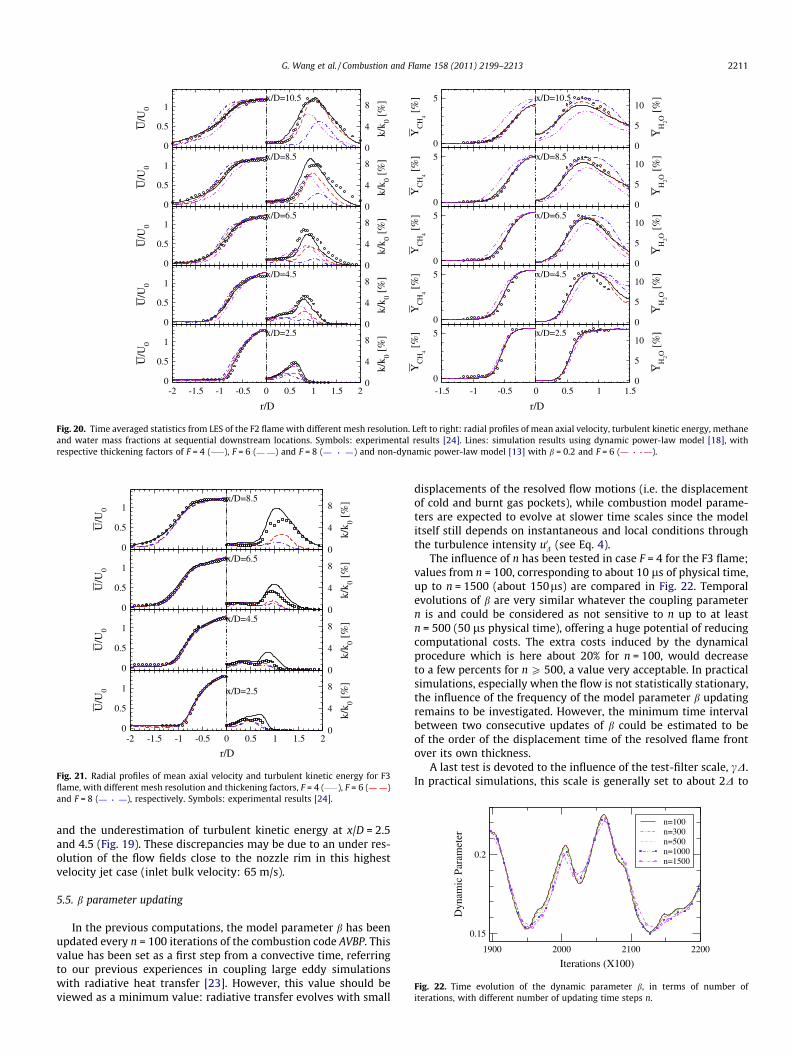
The influence of n has been tested in case F = 4 for the F3 flame;values from n = 100, corresponding to about 10 ls of physical time,up to n = 1500 (about 150ls) are compared in Fig. 22. Temporalevolutions of b are very similar whatever the coupling parametern is and could be considered as not sensitive to n up to at leastn = 500 (50 ls physical time), offering a huge potential of reducingcomputational costs. The extra costs induced by the dynamicalprocedure which is here about 20% for n = 100, would decreaseto a few percents for n P 500, a value very acceptable. In practicalsimulations, especially when the flow is not statistically stationary,the influence of the frequency of the model parameter b updatingremains to be investigated. However, the minimum time intervalbetween two consecutive updates of b could be estimated to beof the order of the displacement time of the resolved flame frontover its own thickness.

A last test is devoted to the influence of the test-filter scale, cD.In practical simulations, this scale is generally set to about 2D to

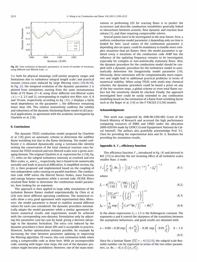
Fig. 23. Time evolution of dynamic parameters, in terms of number of iterations,using different test-filtered scale cD.

2212 G. Wang et al. / Combustion and Flame 158 (2011) 2199–2213

3D, both for physical meanings (self-similar property ranges andlimitations due to turbulence integral length scale) and practicalreasons (extra-costs induced by large filtering sizes) [10,18,19].In Fig. 23, the temporal evolution of the dynamic parameter b isplotted from simulations starting from the same instantaneousfields of F3 flame (F = 4) using three different test-filtered scalescD (c = 2, 2.5 and 3), corresponding to explicit test filter size: 6, 8and 10 mm, respectively according to Eq. (15). b displays a fairlyweak dependency on the parameter c, the difference remaininglower than 10%. This relative insensitivity confirms the validityand robustness of the dynamic thickening flame model in LES prac-tical applications, in agreement with the academic investigation byCharlette et al. [18].

6. Conclusions

The dynamic TFLES combustion model proposed by Charletteet al. [18] gives an automatic scheme to determine the subfilterflame wrinkling lost due to the flame thickening. The model coef-ficient b is obtained dynamically using a Germano-like identitywriting the conservation of the total chemical reaction rates be-tween the TFLES resolved and test-filtered scales over a given aver-aging domain. The original Charlette et al. expression for b [18], Eq.(7), relies on the subgrid turbulence intensity at resolved and testfilter scales, u0D and u0cD, respectively, but is found to be numericallyunstable and leads to practical difficulties. A simplified version, Eq.(9), is then proposed and implemented based on the coupling oftwo independent codes running on parallel machines. The combus-tion code AVBP solves the filtered Navier–Stokes, mass fractionsand energy balance equations while a second code, FILTER, filtersresolved flow fields to determine the combustion model parame-ter, here looking for an exponent.

This approach is then applied to large eddy simulations of theturbulent Bunsen flames studied experimentally by Chen et al.[24] over three different operating conditions. The numerical re-sults show a very good agreement with experimental data. More-over, the model parameter is found to stabilise around differentvalues for each case considered: the dynamic procedure automat-ically adapts the model parameter while a similar agreement be-tween numerical results and experiments would be achievedwith the corresponding non-dynamic formulation only by adjust-ing this parameter case-by-case by hand, giving a decisive advan-tage to the dynamic formalism. The extra cost induced by thedynamic procedure is here about 20% and is acceptable in practice.However, further optimisation remains possible, for example byincreasing the time between parameter updating or improvingthe filtering algorithm. Of course, this cost estimation holds whenusing a compressible code as done here. With an incompressiblecode, running with larger time steps, the cost of the dynamic pro-cedure might become prohibitive. However, one of the main moti-

vations in performing LES for reacting flows is to predict theoccurrence and describe combustion instabilities generally linkedto interactions between acoustic, flow dynamic and reaction heatrelease [1], and then requiring compressible solvers.

Several points have to be investigated in the near future. First, auniform combustion model parameter b depending only on time islooked for here. Local values of the combustion parameter b,depending also on space, could be mandatory to handle more com-plex situations than jet flames. Here, the model parameter is up-dated every n iterations of the combustion code AVBP but theinfluence of the updating frequency remains to be investigated,especially for complex or non-statistically stationary flows. Also,the dynamic procedure for the combustion model should be cou-pled with a dynamic procedure for the turbulence model to auto-matically determine the Smagorinsky model parameter [19].Obviously, these extensions will be computationally more expen-sive and might lead to additional practical problems in terms ofnumerical stability. When using TFLES with multi-step chemicalschemes, the dynamic procedure could be based a priori on anyof the key reaction steps, a global scheme or even total flame sur-face but the sensitivity should be checked. Finally, the approachinvestigated here could be easily extended to any combustionmodelling based on the estimation of a flame front wrinkling factorsuch as the Boger et al. [14] or the F-TACLES [15,50] models.

Acknowledgments

This work was supported by ANR-06-CIS6-002 Grant of theFrench Ministry of Research and accessed the high performancecomputing resources of IDRIS and CINES under the allocation2009-020164 made by GENCI (Grand Equipement National de Cal-cul Intensif). The authors also gratefully acknowledge Prof. Y.C.Chen for providing the experimental data and Dr. E. Knudsen forproviding his simulation results.

Appendix A. CD efficiency function

This efficiency function CD introduced in Eq. (4) and derived inRef. [13] to describe the net straining effect of all turbulent scalessmaller than D reads:

CDD

d0L

;u0DS0

L

;ReD

!¼ ðf�a

u þ f�aD Þ

�1=a �b

þ f�bRe

��1=b

ðA:1Þ

where

fu ¼ 427Ck

110

� �1=2 18Ck

55

� �u0DS0

L

!2

ðA:2Þ

fD ¼27Ckp4=3

110� D

d0L

!4=3

� 1

0@ 1A24 351=2

ðA:3Þ

fRe ¼9

55exp �3

2Ckp4=3Re�1

D

� � �1=2

� Re1=2D : ðA:4Þ

In the above expressions Ck � 1.5 is the Kolmogorov constant. Theexponents a and b control the sharpness of the transitions betweenthe asymptotic behaviours, and good results are obtained with:

a ¼ 0:60þ 0:20 exp �0:1u0DS0

L

!� 0:20 exp �0:01

D

d0L

!; b ¼ 1:4

ðA:5Þ

Since for a laminar flame d0L S0

L=m ¼ 4 [12,13], the subgrid scale Rey-nolds number can be expressed in terms of the two other parame-ters, i.e. ReD ¼ 4 D=d0

L

� �u0D=S0

L

.

G. Wang et al. / Combustion and Flame 158 (2011) 2199–2213 2213

References

[1] T. Poinsot, D. Veynante, Theoretical and Numerical Combustion, second ed.,Edwards Inc., Philadelphia, PA, USA, 2005.

[2] H. Pitsch, Annu. Rev. Fluid Mech. 38 (2006) 453–482.[3] M. Boileau, G. Staffelbach, B. Cuénot, T. Poinsot, C. Bérat, Combust. Flame 154

(1–2) (2008) 2–22.[4] S. Menon, W. Jou, Combust. Sci. Technol. 75 (1–3) (1991) 53–72.[5] S. Roux, G. Lartigue, T. Poinsot, U. Meier, C. Bérat, Combust. Flame 141 (1–2)

(2005) 40–54.[6] T. Schmitt, P. Poinsot, B. Schuermans, K. Geigle, J. Fluid Mech. 570 (2007) 17–

46.[7] S. Richard, O. Colin, O. Vermorel, A. Benkenida, C. Angelberger, D. Veynante,

Proc. Combust. Inst. 31 (2) (2007) 3059–3066.[8] O. Vermorel, S. Richard, O. Colin, C. Angelberger, A. Benkenida, D. Veynante,

Combust. Flame 156 (8) (2009) 1525–1541.[9] V.-K. Chakravarthy, S. Menon, Flow, Turbul. Combust. 65 (2000) 133–161.

[10] E. Knudsen, H. Pitsch, Combust. Flame 154 (2008) 740–760.[11] V. Moureau, B. Fiorina, H. Pitsch, Combust. Flame 156 (4) (2009) 801–812.[12] O. Colin, F. Ducros, D. Veynante, T. Poinsot, Phys. Fluids A 12 (7) (2000) 1843–

1863.[13] F. Charlette, C. Meneveau, D. Veynante, Combust. Flame 131 (1/2) (2002) 159–

180.[14] M. Boger, D. Veynante, H. Boughanem, A. Trouvé, in: Twenty-seventh

Symposium (International) on Combustion, The Combustion Institute, 1998,pp. 917–925.

[15] B. Fiorina, R. Vicquelin, P. Auzillon, N. Darabiha, O. Gicquel, D. Veynante,Combust. Flame 157 (3) (2010) 465–475.

[16] E. Hawkes, S. Cant, Proc. Combust. Inst. 28 (2000) 51–58.[17] H. Weller, G. Tabor, A. Gosman, C. Fureby, in: Twenty-seventh Symposium

(International) on Combustion, The Combustion Institute, 1998, pp. 899–907.[18] F. Charlette, C. Meneveau, D. Veynante, Combust. Flame 131 (1/2) (2002) 181–

197.[19] M. Germano, U. Piomelli, P. Moin, W. Cabot, Phys. Fluids A 3 (7) (1991) 1760–

1765.[20] S.B. Pope, New J. Phys. 6 (2004) 35.[21] A. Stoessel, High-performance computing and networking, in: B. Hertzberger,

G. Serazzi (Eds.), Lecture Notes in Computer Science, vol. 919, Springer-Verlag,Berlin, 1995, pp. 306–311.

[22] H. Boughanem, A. Trouvé, 27th Symposium International on Combustion, Vol.1, The Combustion Institute, 1998, pp. 971–978.

[23] R. Goncalves dos Santos, M. Lecanu, S. Ducruix, O. Gicquel, E. Iacona, D.Veynante, Combust. Flame 152 (3) (2008) 387–400.

[24] Y. Chen, N. Peters, G. Schneemann, N. Wruck, U. Renz, M. Mansour, Combust.Flame 107 (1996) 223–244.

[25] J. Hirschfelder, C. Curtiss, R. Byrd, Molecular Theory of Gases and Liquids, JohnWiley & Sons, New York, 1969.

[26] T. Butler, P. O’Rourke, in: Sixteenth Symposium (International) on Combustion,The Combustion Institute, 1977, pp. 1503–1515.

[27] F. Gouldin, K. Bray, J. Chen, Combust. Flame 77 (1989) 241–259.[28] O. Gulder, in: 23rd Symposium (International) on Combustion, The

Combustion Institute, Pittsburgh, Orléans, 1990, pp. 835–842.[29] www.cerfacs.fr/4-26334-The-AVBP-code.php#avbp.[30] D. You, P. Moin, Phys. Fluids 19 (6).[31] D. You, P. Moin, Phys. Fluids 21 (4).[32] A. Vreman, Phys. Fluids 16 (10) (2004) 3670–3681, doi:10.1063/1.1785131.[33] J. Smagorinsky, Mon. Wea. Rev. 91 (1963) 99–164.[34] J. Légier, D. Veynante, T. Poinsot, in: Proceedings of the Summer Program,

Center for Turbulence Research, 2000.[35] J. Légier, B. Varoquié, F. Lacas, T. Poinsot, D. Veynante, in: A. Pollard, S. Candel

(Eds.), IUTAM Symposium on Turbulent Mixing and Combustion, vol. 70,Kluwer Academic Publishers, 2002, pp. 315–326.

[36] F. Ducros, P. Comte, M. Lesieur, J. Fluid Mech. 326 (1996) 1–36.[37] P. Moin, K. Squires, W. Cabot, S. Lee, Phys. Fluids 113 (1991) 2746–2757.[38] P. Sagaut, R. Grohens, Int. J. Numer. Methods Fluids 31 (1999) 1195–1220.[39] O. Vasilyev, T. Lund, P. Moin, J. Comput. Phys. 146 (1) (1998) 82–104.[40] J. Bentley, J. Friedman, ACM Comput. Surv. 11 (4) (1979) 397–409.[41] H. Kolla, N. Swaminathan, Combust. Flame 157 (7) (2010) 1247–1289.[42] M. Herrmann, Combust. Flame 145 (2006) 357–375.[43] R. Lindstedt, E. Vaos, Combust. Flame 145 (3) (2006) 495–511.[44] H. Pitsch, L. Duchamp de la Geneste, Proc. Combust. Inst. 29 (2002) 2001–2008.[45] A. De, S. Acharya, J. Eng. Gas Turbines Power 131 (061501) (2009) 1–11.[46] E. Van Kalmthout, D. Veynante, Phys. Fluids A 10 (9) (1998) 2347–2368.[47] A. Smirnov, S. Shi, I. Celik, J. Fluids Eng. – Trans. ASME 123 (2) (2001) 359–371.[48] T. Poinsot, S. Lele, J. Comput. Phys. 101 (1) (1992) 104–129.[49] O. Colin, M. Rudgyard, J. Comput. Phys. 162 (2000) 338–371.[50] P. Auzillon, B. Fiorina, R. Vicquelin, N. Darabiha, O. Gicquel, D. Veynante, Proc.

Combust. Inst. 33 (1) (2011) 1331–1338.