implementation issues for hierarchical state estimators · implementation issues for hierarchical...

Implementation Issuesfor Hierarchical State Estimators

Final Project Report

Power Systems Engineering Research Center

Empowering Minds to Engineerthe Future Electric Energy System

Since 1996

PSERC

Implementation Issues for Hierarchical State Estimators

Final Project Report

Project Team

Faculty

Anjan Bose, Project Leader, Washington State University Ali Abur, Northeastern University

Graduate Students

Kai Yin Kenny Poon, Washington State University Roozbeh Emami, Northeastern University

PSERC Document 10-11

August 2010

Information about this project For information about this project contact: Professor Anjan Bose School of Electrical Engineering and Computer Science Washington State University Pullman, WA 99163 Phone: 509-335-1147 Fax: 509-335-3818 Email: [email protected] Power Systems Engineering Research Center This is a project report from the Power Systems Engineering Research Center (PSERC). PSERC is a multi-university center conducting research on challenges facing the electric power industry and educating the next generation of power engineers. More information about PSERC can be found at the center’s website: http://www.pserc.org. For additional information, contact: Power Systems Engineering Research Center Arizona State University 577 Engineering Research Center Tempe, Arizona 85287-5706 Phone: 480-965-1643 Fax: 480-965-0745 Notice Concerning Copyright Material PSERC members are given permission to copy without fee all or part of this publication for internal use if appropriate attribution is given to this document as the source material. This report is available for downloading from the PSERC website.

© 2010 Washington State University All rights reserved

mailto:[email protected]�

http://www.pserc.org/�

i

Acknowledgments

This is the final report for the Power Systems and Engineering Research Center (PSERC) research project S-33 titled “Implementation Issues for Hierarchical State Estimators”. We express our appreciation for the financial support provided by PSERC’s industrial members. The authors also thank PSERC members over the course of this project for their technical advice on this project, especially the industry advisors for this project:

• Lisa Beard – Tennessee Valley Authority • David Bogen – TXU Energy • Floyd Galvan – Entergy Corporation • Jay Giri – Alstom Grid • Jim Graffy – Bonneville Power Administration • Robert Kingsmore – Duke Energy • Shruti Mathure – ITC • Jianzhong Tong – PJM Interconnection • Hui Yang – ITC

ii

Executive Summary

Large interconnections are made up of several reliability coordinators and many balancing authorities. For example, the eastern interconnection has about a dozen reliability coordinators and 100 balancing authorities. Each reliability coordinator and balancing authority has its own control center that uses a state estimator to maintain situation awareness of the internal system, the system over which monitoring and control responsibilities exists. A state estimator for modeling an internal system requires a model of the external system. The state estimator at the reliability coordinator often is a second-level (hierarchical) state estimator that covers several balancing authority areas. Each of these dozens of state estimators has a unique external model that causes the largest errors in real-time models for maintaining situation awareness. In this project, we investigated how the external model affects the accuracy of the state estimator and how the external model can be modified to enhance the state estimator results.

The static database that is used by a state estimator is very costly to maintain because of the data that has to be obtained from neighboring utilities. Many control centers are trying to address the issue of database costs with various levels of data exchange with their neighbors. However, the philosophy of keeping a fixed external model for a state estimator remains. Furthermore, the largest real-time model is still much smaller than the whole interconnection.

There is renewed interest in situation awareness for an entire interconnection because of the cascading blackout of August 2003 which affected an area that is not covered by any one control center. In fact, a recent DOE/FERC report on the monitoring of the entire North American grid recommends use of interconnection-wide monitoring centers. As cited in the report, such centers will be made possible when enough phasor measurement units for time-synchronizing the data exist across an interconnection. Operationally, the local monitoring and state estimation results can be moved up through the reliability coordinators to an interconnection-wide monitoring center. If the use of interconnection-wide monitoring centers becomes feasible, the financial and reliability benefits will be quite substantial. Another real benefit will be that a real-time model of the whole interconnection could also be made available for local decision-making.

The feasibility of solving a hierarchical and distributed state estimator has mainly been studied from an algorithmic-solution viewpoint. The rich research literature on state estimation shows that such state estimators can be solved. The actual implementation of a state estimator, however, depends on many other factors, such as

iii

the time skew of the data that basically unsynchronizes the data in the state estimation process, the accuracy of the network database, the availability of raw data versus state-estimated data, and sensitive issues regarding the proprietary nature of the data.

Two parallel investigation paths were pursued in our research.

1. The first path was to investigate the effect of exchanging more real-time measurement data between the external model and the state estimator. This also included investigating the retention of more detailed external models than the present day practice of only retaining equivalents at the boundary buses.

2. The second path was to investigate the effect of utilizing synchronized phasor measurements from the external model in the state estimator. This also included investigating the optimal positioning of the synchrophasors in the external model.

The overall conclusion is that state estimator results improve directly in proportion to the amount of real-time data exchanged. Also, if more data is exchanged, the external model can be represented in more detail than the present practice of equivalencing at the boundary. The phasor measurements have the added advantage of being time-stamped. If such synchrophasor data from the external model can be compared with synchrophasor data in the internal system, then the errors due to time-skews can be controlled.

Most of the testing done in this project was done on the IEEE 118-bus system. The next step is to test our approach to hierarchical, distributed state estimation on a real system. A plan was developed to study the TVA-Entergy system since TVA and Entergy are PSERC members who are neighbors and each of their state estimators model the others’ system in their external models. However, the work required to do the testing was more than could be accomplished in this project in part because TVA-Entergy use external models that are equivalenced at their boundary buses, and these equivalents were determined from planning (node-branch) models rather than EMS (circuit breaker-bus section) models. The testing phase could be accomplished in future research with close cooperation of utility personnel who are familiar with the details of the target power system.

iv

Table of Contents

1 Introduction ........................................................................................................ 1 1.1 Background ............................................................................................ 1 1.2 Project objectives and description ......................................................... 2

2 Effects of data exchange on internal state estimation ........................................ 3 2.1 Introduction ............................................................................................ 3 2.2 Methodology .......................................................................................... 3

2.2.1 Modeling of external power system in power system state estimators ................................................................................... 3

2.2.2 Approach .................................................................................... 4 2.3 Experiments on data exchange ............................................................... 5

2.3.1 IEEE 118 bus system test bed .................................................... 5 2.3.2 Preliminary studies of trends ..................................................... 6 2.3.3 Study of effects of loss of communications ............................... 8 2.3.4 Further investigation on the effects of loss of communication

on state estimators .................................................................... 10 2.3.5 Exchanging SCADA data VS exchanging state estimated

data ........................................................................................... 13 2.4 Summary .............................................................................................. 25

3 Impact of external system measurements on internal state estimation ............ 26 3.1 Introduction .......................................................................................... 26 3.2 Effect of using external system synchronized phasor measurements on

internal system state estimation solution ............................................. 28 3.2.1 Problem formulation ................................................................ 28

3.3 Simulation results ................................................................................. 30 3.3.1 Impact of external measurements on state estimation ............. 30 3.3.2 Effect of PMUs on real-time contingency analysis ................. 32

3.4 Optimal choice of external measurements ........................................... 34 3.4.1 Problem formulation ................................................................ 34 3.4.2 Simulation results..................................................................... 39

4 Conclusions ...................................................................................................... 44

v

List of Figures

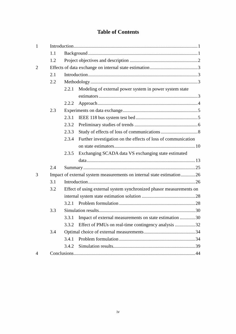
Figure 2.1: Schematics of interconnected system ....................................................... 4Figure 2.2: IEEE 118 bus system diagram under configuration 1 .............................. 9Figure 2.3: IEEE 118 bus system diagram under configuration 2 ............................ 11Figure 3.1: Schematic of an interconnected system .................................................. 29Figure 3.2: Reordered S matrix ................................................................................. 36Figure 3.3: Flow chart of the algorithm .................................................................... 39

vi

List of Tables

Table 2.1: List of scenarios representing various levels of data exchange ................. 6Table 2.2: Results for study of effects of data exchange on internal state estimation in the event of generation pattern shifts ......................................................................... 7Table 2.3: Details of IEEE 118 bus system under configuration 1 ............................. 9Table 2.4: Results on study of loss of communication for IEEE 118 bus system (Configuration 1) ........................................................................................................... 9Table 2.5: Results on study of loss of communication for IEEE 118 bus system for topology change on like 49-66 (Configuration 1) ........................................................ 10Table 2.6: Details of IEEE 118 bus system under Configuration 1 .......................... 11Table 2.7: Results for Study of Loss of Communication for IEEE 118 bus system (Configuration 2) ......................................................................................................... 12Table 2.8: Results for Specific Cases in Study of Loss of Communication for IEEE 118 bus system (Configuration 2) ................................................................................ 13Table 2.9: Details of buses in IEEE 118 bus system (Configuration 1) .................... 15Table 2.10: Details of buses in IEEE 118 bus system (Configuration 2) .................. 15Table 2.11: List of scenarios for comparison of effects of various types and levels of data exchange on internal state estimation ................................................................... 16Table 2.12: Results for Study of Exchange of SCADA data VS State estimated data (Configuration 1) ......................................................................................................... 17Table 2.13: Results for Study of Exchange of SCADA data VS State estimated data (Configuration 1) ......................................................................................................... 18Table 2.14: Results for Study of Exchange of SCADA data VS State estimated data (Configuration 1) ......................................................................................................... 19Table 2.15: Results for Study of Exchange of SCADA data VS State estimated data (Configuration 2) ......................................................................................................... 20Table 2.16: Results for Study of Exchange of SCADA data VS State estimated data (Configuration 2) ......................................................................................................... 21Table 2.17: Results for Study of Exchange of SCADA data VS State estimated data under the Effects of Topology Errors (Configuration 1) .............................................. 22Table 2.18: Results for Study of Exchange of SCADA data VS State estimated data under the Effects of Topology Errors (Configuration 1) .............................................. 23Table 2.19: Results for Study of Exchange of SCADA data VS State estimated data under the Effects of Topology Errors (Configuration 2) .............................................. 24Table 3.1: 118-Bus Example: Internal and External System Buses .......................... 31Table 3.2: List of PMUs and the corresponding accuracy metric, J. ........................ 32Table 3.3: List of PMUs and the corresponding accuracy metric, Jc. ....................... 34

vii

List of Tables (continued)

Table 3.4: Chi square values for different choices of accuracy tolerance ε. ............. 40Table 3.5: Error Metric of (12) ................................................................................. 41Table 3.6: Error metric of (13) for contingency case ................................................ 42

1

1 Introduction

1.1 Background

The control and operation of power systems is based on the ability to determine the state of the system in real time, and this requires monitoring of the system operating conditions in real time. Conventionally, this is performed by the state estimator in the control center which has access to measurements from monitored areas by the control center.

Nowadays, large interconnections comprise several reliability coordinators (RC) and many balancing authorities (BA), each having their own control center. The state estimator at the RC is often a two level (hierarchical) state estimator monitoring several BA areas. Each of these state estimators at an RC has a unique external model, and the static data base for these external models is costly to maintain because of the data which has to be obtained from neighboring utilities. Moreover, the external models are also the largest source of errors in the real time model.

One way to address this issue is to incorporate various levels of data exchange between control centers. However, the issue that each control center possesses its own external model remains, and the fact is that the largest real time model in a control center is small compared to the whole interconnection. A recent DOE/FERC report on the monitoring of the whole North American grid recommends a monitoring center for the entire interconnection and cites the availability of sufficient phasor measurement units (PMUs) to provide for time synchronization of the data. There are numerous financial and reliability benefits for such a monitoring center, one of which is that the local SE results can be moved up through to the reliability coordinators to a central monitoring center, such that the real time model of the entire interconnection would be available to the lower entities for better local decision making.

There have been studies of a hierarchical and distributed state estimator in the literature [3]-[7], but the majority of these studies have been from an algorithmic solution viewpoint, and it has been shown that such hierarchical and distributed state estimators are successful in obtaining solutions. However, it is worth noting that there are numerous factors which would have to be taken into consideration for the actual implementation of a hierarchical and distributed state estimator. Such factors range from technical issues such as the time skew of the data, the accuracy of the network data base to other issues including the proprietary nature of the data. In this project,

2

some of these issues are studied to determine requirements to render such a hierarchical and distributed state estimator feasible.

1.2 Project objectives and description

As mentioned in the previous section, the objective of this project is to research the aforementioned issues relevant to making a hierarchical and distributed state estimator feasible. The approach in this project will be to make use of state estimator programs to perform simulations and study the feasibility of such a hierarchical and distributed state estimator. The focus of the study is on data issues, such as the amount of data required from external systems and the study of movement for both SCADA data and state estimated data.

In this project, the study will be performed for scenarios assuming both detailed external models and reduced external models. The effects of data exchange will be studied for the scenario where the full model is used. Issues such as the amount of data to be exchanged and the exchange of state estimated data versus SCADA data are investigated. Moreover, consideration of the loss of communication with neighboring areas will be included and their effects on the internal state estimation are then observed.

Another aspect of the project is to observe the effects of a few external system measurements on internal state estimation, and the formulation of the external system model in such cases will also be discussed. In addition to determining the effects of external measurements on internal state estimation, the study on the effects of PMUs on real-time contingency analysis is also performed. Finally, the study on the optimal choice of external measurements is also conducted by formulating the external system measurement selection as a mixed integer programming problem.

This report is organized in four sections. The effects of large changes in the external system on internal state estimation are investigated in section 2. The modeling of the external system and approaches are first described, and then the effects of exchanging different types of data on state estimation are then presented. Section 3 contains details on the impact of several external system measurements on internal state estimation. The effects of incorporating PMUs on real-time contingency analysis are also investigated, and finally the study of external system measurement selection is performed. Conclusions and final remarks are drawn in Section 4 of the report.

3

2 Effects of data exchange on internal state estimation

2.1 Introduction

In this section, the effects of large changes in the external system on internal state estimation are investigated. Common examples of such large changes include topology changes and generation pattern shifts. The effects of loss of communication in parts of the external system on internal state estimation accuracy are then studied.

Finally, the effect of performing various amounts and types of data exchange with neighboring areas (using conventional measurements) on the improvement of internal state estimation accuracy is investigated. Various scenarios are created to simulate changes in system operation which may occur in real systems, and simulations are conducted to compare the accuracy of internal state estimation under these different scenarios.

2.2 Methodology

2.2.1 Modeling of external power system in power system state estimators

In performing state estimation, it is inherent that sufficient measurements are available to ensure that the system is observable. In large interconnected systems, each utility has detailed information regarding the operating conditions in its own control area. However, in the absence of data exchange, the external parts of the interconnected system remain unobservable, and various EMS functions cannot be performed without taking into consideration the external system. The portion of the interconnected system which is outside a utility’s control area is known as the external network model.

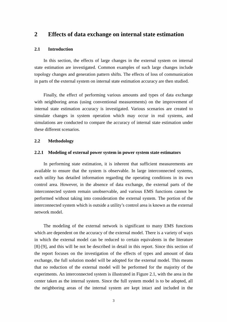
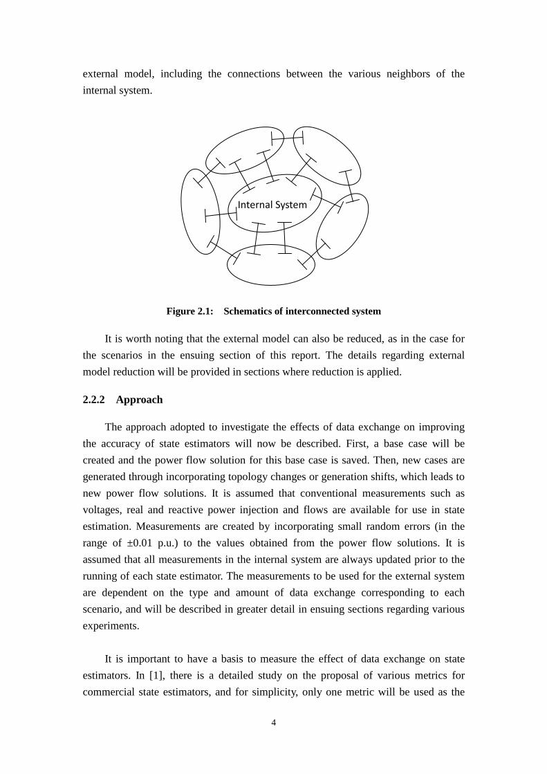
The modeling of the external network is significant to many EMS functions which are dependent on the accuracy of the external model. There is a variety of ways in which the external model can be reduced to certain equivalents in the literature [8]-[9], and this will be not be described in detail in this report. Since this section of the report focuses on the investigation of the effects of types and amount of data exchange, the full solution model will be adopted for the external model. This means that no reduction of the external model will be performed for the majority of the experiments. An interconnected system is illustrated in Figure 2.1, with the area in the center taken as the internal system. Since the full system model is to be adopted, all the neighboring areas of the internal system are kept intact and included in the

4

external model, including the connections between the various neighbors of the internal system.

Figure 2.1: Schematics of interconnected system

It is worth noting that the external model can also be reduced, as in the case for the scenarios in the ensuing section of this report. The details regarding external model reduction will be provided in sections where reduction is applied.

2.2.2 Approach

The approach adopted to investigate the effects of data exchange on improving the accuracy of state estimators will now be described. First, a base case will be created and the power flow solution for this base case is saved. Then, new cases are generated through incorporating topology changes or generation shifts, which leads to new power flow solutions. It is assumed that conventional measurements such as voltages, real and reactive power injection and flows are available for use in state estimation. Measurements are created by incorporating small random errors (in the range of ±0.01 p.u.) to the values obtained from the power flow solutions. It is assumed that all measurements in the internal system are always updated prior to the running of each state estimator. The measurements to be used for the external system are dependent on the type and amount of data exchange corresponding to each scenario, and will be described in greater detail in ensuing sections regarding various experiments.

It is important to have a basis to measure the effect of data exchange on state estimators. In [1], there is a detailed study on the proposal of various metrics for commercial state estimators, and for simplicity, only one metric will be used as the

Internal System

5

basis to illustrate and compare the accuracy of state estimators under different scenarios in this chapter. The metric to be used in all experiments in this chapter is denoted by J and is given by the following equation:

( ) ( )1

1 NPF PF

i i i ii

J V V V VN

∗

=

= − − ∑

where iV

is the estimated complex voltage at bus i

PFiV

is the complex voltage at bus i based on power flow solution

The above metric takes the difference between the estimated complex voltage and the exact complex voltage at each bus, and multiples this value by its complex conjugate to obtain a real number. The sum of these real numbers obtained for each internal system bus is then divided by the number of internal system buses.

It is worth noting that while the above metric provides a general idea on the accuracy of internal state estimation, there is the possibility that the metric can be misleading in the event that there is a sufficiently large error at a single bus, which would lead to a large increase in the value obtained by the metric to give the impression that there is a large error spread throughout the whole system. On the other hand, it is also possible that an error at a boundary bus might be hidden by the value of the metric if the number of buses is large enough. Intuitively, it is expected that the errors in internal state estimation would appear at the boundary buses, and therefore, the errors at the boundary buses of the internal system are also checked for each scenario. In the ensuing subsections, the errors will be illustrated in cases where it is necessary to provide greater insight to understanding the effects of data exchange on internal state estimation.

2.3 Experiments on data exchange

2.3.1 IEEE 118 bus system test bed

The IEEE 118 bus system is adopted as the test bed for performing simulations in the investigation of data exchange for state estimators. The system is then partitioned into subsystems, with each subsystem representing the area owned by a reliability coordinator. For the convenience of the reader, Area 1 will be assumed to be the internal system while other areas will be considered as external systems. The

6

detailed system model will be adopted for the external system model, and pseudomeasurements will be used where necessary to ensure that the system remains observable. Preliminary studies will be carried out to observe trends regarding the effects of different levels of data exchange on the performance of internal state estimation when there are changes in system operation conditions. In general, there are two types of events in real power systems which lead to large changes in system operation conditions. The first is the occurrence of topology changes in the system which lead to changes in the power flow solution, and the second is a shift in generation pattern as a result of the scheduling of generators which causes certain generators to either start up or shut down over the course of the day. Changes in load over the course of the day will not be considered in this section, but will be addressed later in this report.

2.3.2 Preliminary studies of trends

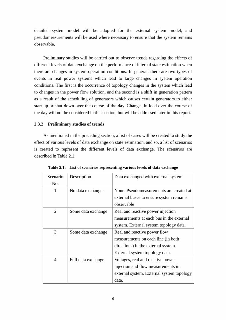
As mentioned in the preceding section, a list of cases will be created to study the effect of various levels of data exchange on state estimation, and so, a list of scenarios is created to represent the different levels of data exchange. The scenarios are described in Table 2.1.

Table 2.1: List of scenarios representing various levels of data exchange

Scenario No.

Description Data exchanged with external system

1 No data exchange. None. Pseudomeasurements are created at external buses to ensure system remains observable

2 Some data exchange Real and reactive power injection measurements at each bus in the external system. External system topology data.

3 Some data exchange Real and reactive power flow measurements on each line (in both directions) in the external system. External system topology data.

4 Full data exchange Voltages, real and reactive power injection and flow measurements in external system. External system topology data.

7

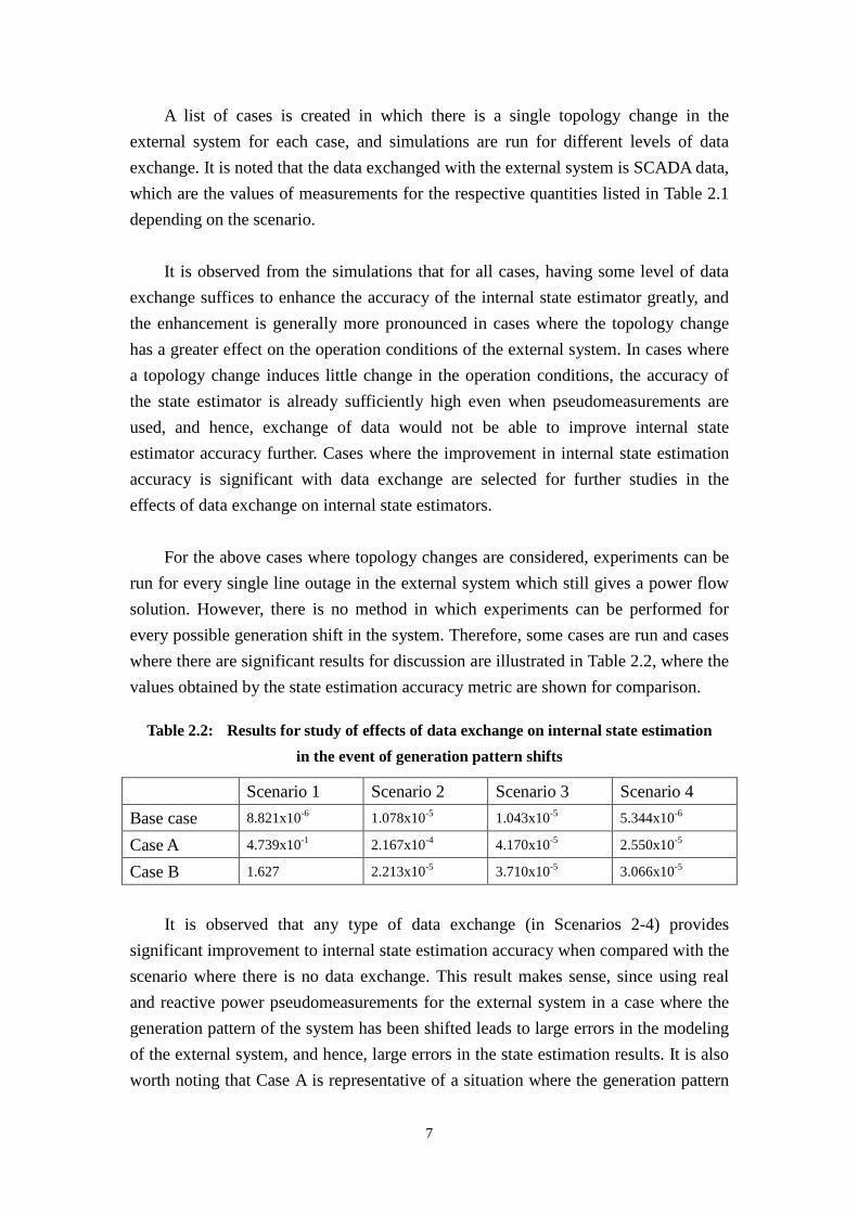
A list of cases is created in which there is a single topology change in the external system for each case, and simulations are run for different levels of data exchange. It is noted that the data exchanged with the external system is SCADA data, which are the values of measurements for the respective quantities listed in Table 2.1 depending on the scenario. It is observed from the simulations that for all cases, having some level of data exchange suffices to enhance the accuracy of the internal state estimator greatly, and the enhancement is generally more pronounced in cases where the topology change has a greater effect on the operation conditions of the external system. In cases where a topology change induces little change in the operation conditions, the accuracy of the state estimator is already sufficiently high even when pseudomeasurements are used, and hence, exchange of data would not be able to improve internal state estimator accuracy further. Cases where the improvement in internal state estimation accuracy is significant with data exchange are selected for further studies in the effects of data exchange on internal state estimators. For the above cases where topology changes are considered, experiments can be run for every single line outage in the external system which still gives a power flow solution. However, there is no method in which experiments can be performed for every possible generation shift in the system. Therefore, some cases are run and cases where there are significant results for discussion are illustrated in Table 2.2, where the values obtained by the state estimation accuracy metric are shown for comparison.

Table 2.2: Results for study of effects of data exchange on internal state estimation in the event of generation pattern shifts

Scenario 1 Scenario 2 Scenario 3 Scenario 4 Base case 8.821x10-6 1.078x10-5 1.043x10-5 5.344x10-6

Case A 4.739x10-1 2.167x10-4 4.170x10-5 2.550x10-5

Case B 1.627 2.213x10-5 3.710x10-5 3.066x10-5

It is observed that any type of data exchange (in Scenarios 2-4) provides

significant improvement to internal state estimation accuracy when compared with the scenario where there is no data exchange. This result makes sense, since using real and reactive power pseudomeasurements for the external system in a case where the generation pattern of the system has been shifted leads to large errors in the modeling of the external system, and hence, large errors in the state estimation results. It is also worth noting that Case A is representative of a situation where the generation pattern

8

shifts slightly, while Case B represents a situation where there is a large shift in the generation pattern. In fact, by observation of the metric obtained in Case B, it can be seen that the state estimator does not even provide a reasonable result, which intuitively leads us to believe that it is possible that internal state estimation can fail to obtain a reasonable result for power systems in the events where the modeling of external model is sufficiently erroneous. The difference in accuracy for the various scenarios where data exchange is implemented is very small, since there is a high level of redundancy for all these cases. In scenarios where some data exchange already leads to a state estimation solution which is basically correct, total data exchange does not necessarily improve accuracy any further because of random errors which lie in every measurement in the system.

2.3.3 Study of effects of loss of communications

Based on the preliminary studies, it is observed that data exchange helps provide improvements in state estimator accuracy and in this subsection, the effects of loss of communication with a portion of the external system on internal state estimation are investigated.

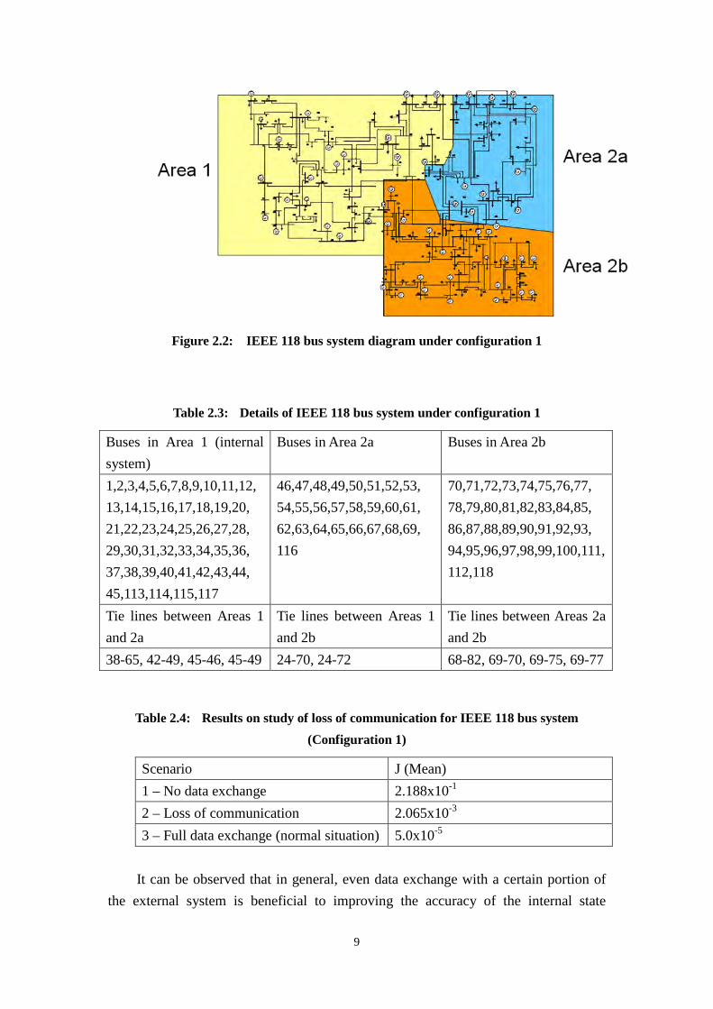
The external system is further divided into two areas as shown in Figure 2.2, and for simplicity, these two areas are named Area 2A and Area 2B. Details of this configuration of the IEEE 118 bus system are also provided in Table 2.3. For the purpose of the investigation in this part, three scenarios are created for the comparison of internal state estimator accuracy. In the first scenario, there is no data exchange at all, and pseudomeasurements are used in the entire external system to ensure the system remains observable. In the second scenario, the loss of communication is modeled by having data exchange with Area 2A, while pseudomeasurements are used for Area 2B to ensure the system remains observable. Finally, in the third scenario, full data exchange (voltages, real and reactive power injection and flow measurements in external system) is implemented. The mean values of the accuracy metric are taken for all the cases and illustrated in Table 2.4.

9

Figure 2.2: IEEE 118 bus system diagram under configuration 1

Table 2.3: Details of IEEE 118 bus system under configuration 1

Buses in Area 1 (internal system)

Buses in Area 2a Buses in Area 2b

1,2,3,4,5,6,7,8,9,10,11,12, 13,14,15,16,17,18,19,20, 21,22,23,24,25,26,27,28, 29,30,31,32,33,34,35,36, 37,38,39,40,41,42,43,44, 45,113,114,115,117

46,47,48,49,50,51,52,53, 54,55,56,57,58,59,60,61, 62,63,64,65,66,67,68,69, 116

70,71,72,73,74,75,76,77, 78,79,80,81,82,83,84,85, 86,87,88,89,90,91,92,93, 94,95,96,97,98,99,100,111,112,118

Tie lines between Areas 1 and 2a

Tie lines between Areas 1 and 2b

Tie lines between Areas 2a and 2b

38-65, 42-49, 45-46, 45-49 24-70, 24-72 68-82, 69-70, 69-75, 69-77

Table 2.4: Results on study of loss of communication for IEEE 118 bus system (Configuration 1)

Scenario J (Mean) 1 – No data exchange 2.188x10-1

2 – Loss of communication 2.065x10-3

3 – Full data exchange (normal situation) 5.0x10-5

It can be observed that in general, even data exchange with a certain portion of

the external system is beneficial to improving the accuracy of the internal state

10

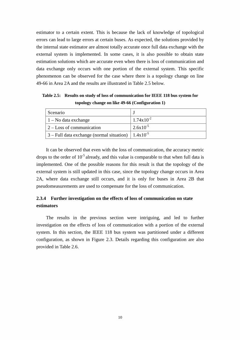
estimator to a certain extent. This is because the lack of knowledge of topological errors can lead to large errors at certain buses. As expected, the solutions provided by the internal state estimator are almost totally accurate once full data exchange with the external system is implemented. In some cases, it is also possible to obtain state estimation solutions which are accurate even when there is loss of communication and data exchange only occurs with one portion of the external system. This specific phenomenon can be observed for the case where there is a topology change on line 49-66 in Area 2A and the results are illustrated in Table 2.5 below.

Table 2.5: Results on study of loss of communication for IEEE 118 bus system for topology change on like 49-66 (Configuration 1)

Scenario J 1 – No data exchange 1.74x10-2

2 – Loss of communication 2.6x10-5

3 – Full data exchange (normal situation) 1.4x10-5

It can be observed that even with the loss of communication, the accuracy metric

drops to the order of 10-5 already, and this value is comparable to that when full data is

implemented. One of the possible reasons for this result is that the topology of the external system is still updated in this case, since the topology change occurs in Area 2A, where data exchange still occurs, and it is only for buses in Area 2B that pseudomeasurements are used to compensate for the loss of communication.

2.3.4 Further investigation on the effects of loss of communication on state estimators

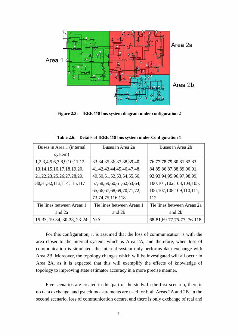
The results in the previous section were intriguing, and led to further investigation on the effects of loss of communication with a portion of the external system. In this section, the IEEE 118 bus system was partitioned under a different configuration, as shown in Figure 2.3. Details regarding this configuration are also provided in Table 2.6.

11

Figure 2.3: IEEE 118 bus system diagram under configuration 2

Table 2.6: Details of IEEE 118 bus system under Configuration 1

Buses in Area 1 (internal system)

Buses in Area 2a Buses in Area 2b

1,2,3,4,5,6,7,8,9,10,11,12, 13,14,15,16,17,18,19,20, 21,22,23,25,26,27,28,29, 30,31,32,113,114,115,117

33,34,35,36,37,38,39,40, 41,42,43,44,45,46,47,48, 49,50,51,52,53,54,55,56, 57,58,59,60,61,62,63,64, 65,66,67,68,69,70,71,72, 73,74,75,116,118

76,77,78,79,80,81,82,83, 84,85,86,87,88,89,90,91, 92,93,94,95,96,97,98,99, 100,101,102,103,104,105,106,107,108,109,110,111, 112

Tie lines between Areas 1 and 2a

Tie lines between Areas 1 and 2b

Tie lines between Areas 2a and 2b

15-33, 19-34, 30-38, 23-24 N/A 68-81,69-77,75-77, 76-118

For this configuration, it is assumed that the loss of communication is with the area closer to the internal system, which is Area 2A, and therefore, when loss of communication is simulated, the internal system only performs data exchange with Area 2B. Moreover, the topology changes which will be investigated will all occur in Area 2A, as it is expected that this will exemplify the effects of knowledge of topology to improving state estimator accuracy in a more precise manner.

Five scenarios are created in this part of the study. In the first scenario, there is no data exchange, and psuedomeasurements are used for both Areas 2A and 2B. In the second scenario, loss of communication occurs, and there is only exchange of real and

12

reactive power injection data with Area 2B, while psuedomeasurements are used where necessary in Area 2A to ensure the system remains observable. In scenario 3, the loss of communication is simulated once again, but the data exchange involves real and reactive line flows in Area 2B. In scenario 4, the normal situation where there is data exchange with both Area 2A and Area 2B is simulated, and real and reactive power injection data are exchanged with Areas 2A and 2B. Finally, in scenario 5, full data exchange is implemented where all measurements in Areas 2A and 2B are exchanged. The mean values of the state estimation accuracy metric for all cases are illustrated in Table 2.7.

Table 2.7: Results for Study of Loss of Communication for IEEE 118 bus system (Configuration 2)

Scenario J (Mean) 1 1.85x10-2

2 1.86x10-2

3 2.304x10-2 4 6.15x10-5 5 1.97x10-5

For this configuration, it is observed that even having data exchange with parts

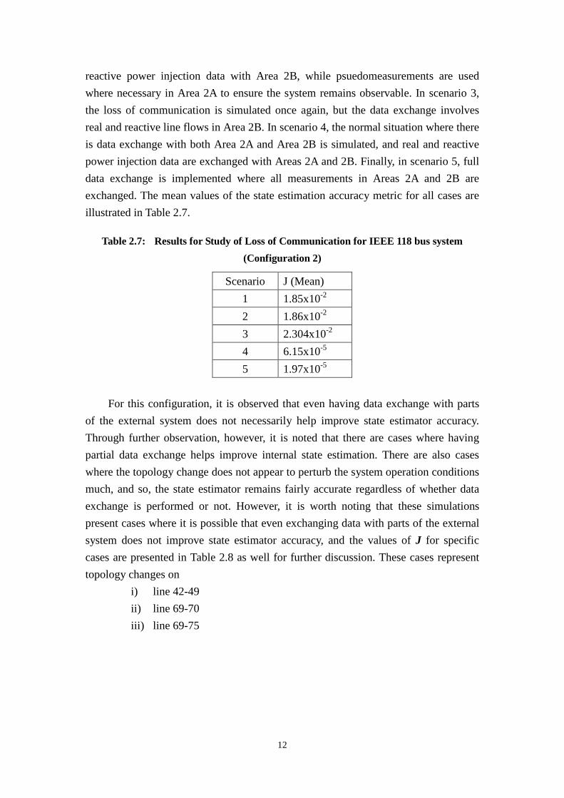
of the external system does not necessarily help improve state estimator accuracy. Through further observation, however, it is noted that there are cases where having partial data exchange helps improve internal state estimation. There are also cases where the topology change does not appear to perturb the system operation conditions much, and so, the state estimator remains fairly accurate regardless of whether data exchange is performed or not. However, it is worth noting that these simulations present cases where it is possible that even exchanging data with parts of the external system does not improve state estimator accuracy, and the values of J for specific cases are presented in Table 2.8 as well for further discussion. These cases represent topology changes on

i) line 42-49 ii) line 69-70 iii) line 69-75

13

Table 2.8: Results for Specific Cases in Study of Loss of Communication for IEEE 118 bus system (Configuration 2)

Scenario J (line 42-49) J (line 69-70) J (line 69-75) 1 2.102x10-1 7.949x10-2 1.824x10-2 2 2.097x10-1 7.811x10-2 1.907x10-2 3 2.595x10-1 8.574x10-2 4.155x10-2 4 9.96x10-5 9.06x10-5 1.16x10-5 5 2.04x10-5 1.15x10-5 1.62x10-5

It can be observed for these cases that the loss of communication with a certain

part of the external network is critical, since it leads to large errors in internal state estimation. One of the reasons is that for these cases, the topology data is incorrect, as the loss of communication with Area 2A causes topology changes in that area to become unknown to the internal state estimator. This shows that greater knowledge of analog data may not have any effect on improving the accuracy of internal state estimators while the lack of knowledge of topology data can lead to large errors in state estimation results at certain buses.

2.3.5 Exchanging SCADA data VS exchanging state estimated data

In the previous sections, it has been assumed that SCADA data exchange is implemented in scenarios where data exchange occurs, and this data comprises measurements from the external system. In this section, the comparison between exchange of SCADA data and state estimated data for state estimators will be studied. The cases set up for this study are similar to those in previous section, such that topology changes in the external system will be created and various scenarios representing different levels or types of data exchange will be used and the accuracy of internal state estimation will then be observed.

As mentioned in previous sections, the detailed system model is adopted for the external network when SCADA data exchange is implemented. In the event where state estimated data is exchanged, a reduced model will be adopted for the external system. The method in which this reduced external model is obtained is briefly explained here. First, consider Area 1 as the internal system, which would obtain state estimated data from Area 2 during data exchange. This data contains information about all the voltages and angles at each bus in Area 2, from which the corresponding real and reactive power injections and flows in Area 2 can be calculated. The external system will be reduced up to the boundary buses connected to Area 1 through tie

14

lines.

Based on the state estimated solution of Area 2, the modified real and reactive power injections at the external boundary buses can be obtained by accounting for line flows connected to these buses. The corresponding process can be performed when Area 2 obtains state estimated data from Area 1 to run its own state estimator. The modified real and reactive power injection measurements created at these external boundary buses based on the external system’s state estimation solutions are considered to have a very high confidence level. Such a setting provides the effect of fixing the values of the measurements at these external boundary buses during internal state estimation.

The process for simulating exchange of state estimated data is now described. Area 1 is considered as the internal system.

i) The internal state estimator for Area 1 is solved first, and this solution is sent to Area 2.

ii) Area 2 then runs its state estimator based on its own internal measurements and Area 1’s state estimated data, and sends this SE solution back to Area 1.

iii) Finally, Area 1 makes use of this new set of state estimated data from Area 2 to perform internal state estimation again, and the value of the state estimation accuracy metric is obtained and used for comparison with other scenarios.

It is important to mention that the data used to perform step (i) of the above

process is dependent on events happening in the power system. Specifically, the data to be used is dependent on the time that the topology change occurs. First, it is possible that the topology change occurs prior to the time Area 1 receives Area 2’s state estimated data, such that the topology data which Area 1 obtains would already be correct. The other possibility is for the topology change to occur after Area 1 receives Area 2’s state estimated data, such that the data Area 1 obtains is not up to date. In running the experiments both possibilities are considered, and the former situation would be considered as the case where Area 1 obtains updated data at the beginning, while the latter situation would be nominated as the case where Area 1 obtains data which is not up to date. For the purpose of this study, the topology change is assumed to always occur before step (ii) of the process. Therefore, by step (ii), the topology change has already occurred, and this will be known by Area 1 for its internal state estimation in step (iii).

15

The above possibilities do not occur for SCADA data exchange, since this type

of data exchange only requires one step, as the measurements are exchanged directly. Hence, whenever SCADA data is exchanged between state estimators, it is assumed that topology data is sent as well.

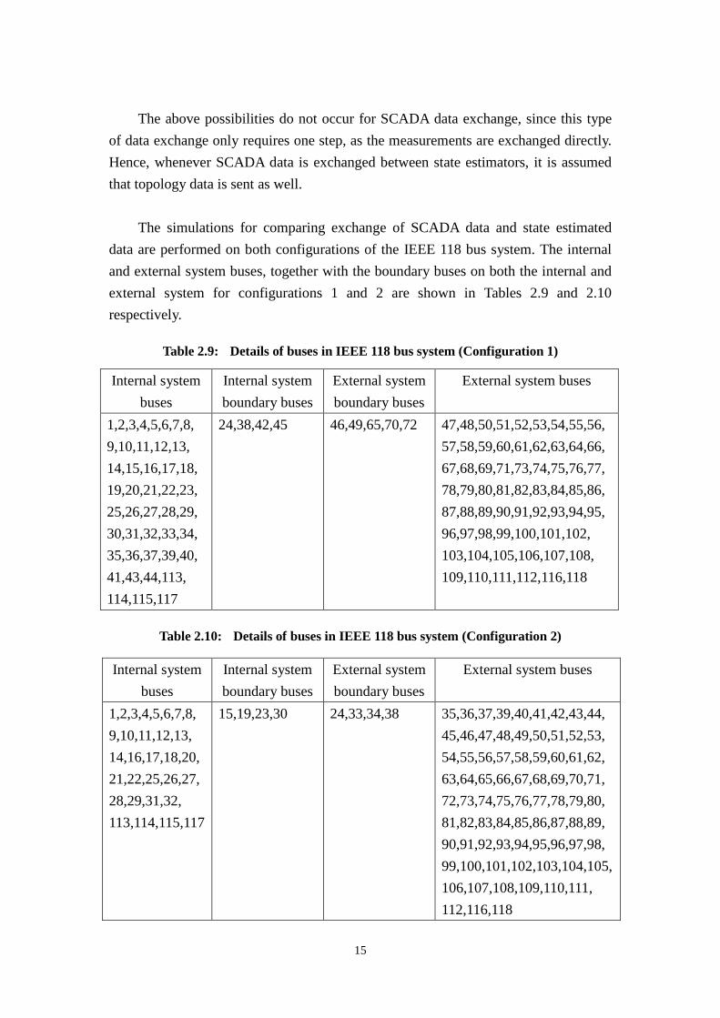
The simulations for comparing exchange of SCADA data and state estimated data are performed on both configurations of the IEEE 118 bus system. The internal and external system buses, together with the boundary buses on both the internal and external system for configurations 1 and 2 are shown in Tables 2.9 and 2.10 respectively.

Table 2.9: Details of buses in IEEE 118 bus system (Configuration 1)

Internal system buses

Internal system boundary buses

External system boundary buses

External system buses

1,2,3,4,5,6,7,8, 9,10,11,12,13, 14,15,16,17,18, 19,20,21,22,23, 25,26,27,28,29, 30,31,32,33,34, 35,36,37,39,40, 41,43,44,113, 114,115,117

24,38,42,45 46,49,65,70,72 47,48,50,51,52,53,54,55,56, 57,58,59,60,61,62,63,64,66, 67,68,69,71,73,74,75,76,77, 78,79,80,81,82,83,84,85,86, 87,88,89,90,91,92,93,94,95, 96,97,98,99,100,101,102, 103,104,105,106,107,108, 109,110,111,112,116,118

Table 2.10: Details of buses in IEEE 118 bus system (Configuration 2)

Internal system buses

Internal system boundary buses

External system boundary buses

External system buses

1,2,3,4,5,6,7,8, 9,10,11,12,13, 14,16,17,18,20, 21,22,25,26,27, 28,29,31,32, 113,114,115,117

15,19,23,30 24,33,34,38 35,36,37,39,40,41,42,43,44, 45,46,47,48,49,50,51,52,53, 54,55,56,57,58,59,60,61,62, 63,64,65,66,67,68,69,70,71, 72,73,74,75,76,77,78,79,80, 81,82,83,84,85,86,87,88,89, 90,91,92,93,94,95,96,97,98, 99,100,101,102,103,104,105, 106,107,108,109,110,111, 112,116,118

16

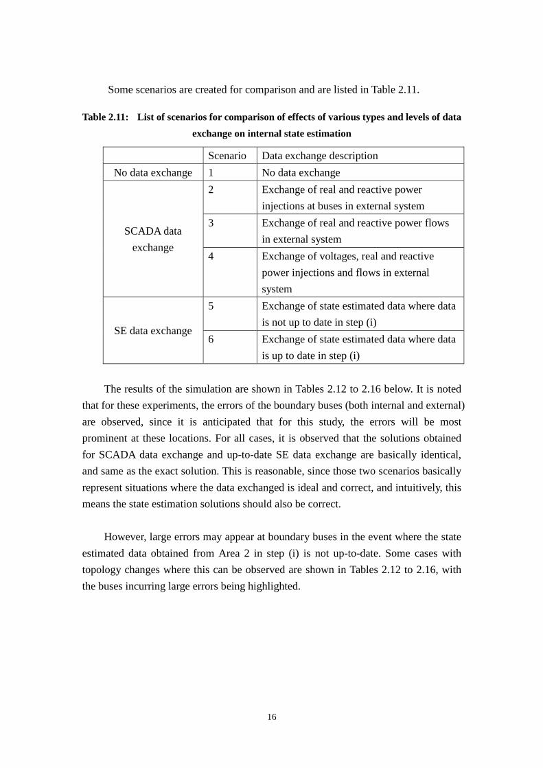
Some scenarios are created for comparison and are listed in Table 2.11.

Table 2.11: List of scenarios for comparison of effects of various types and levels of data exchange on internal state estimation

Scenario Data exchange description No data exchange 1 No data exchange

SCADA data exchange

2 Exchange of real and reactive power injections at buses in external system

3 Exchange of real and reactive power flows in external system

4 Exchange of voltages, real and reactive power injections and flows in external system

SE data exchange

5 Exchange of state estimated data where data is not up to date in step (i)

6 Exchange of state estimated data where data is up to date in step (i)

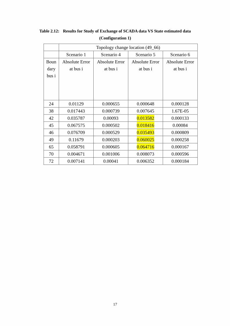
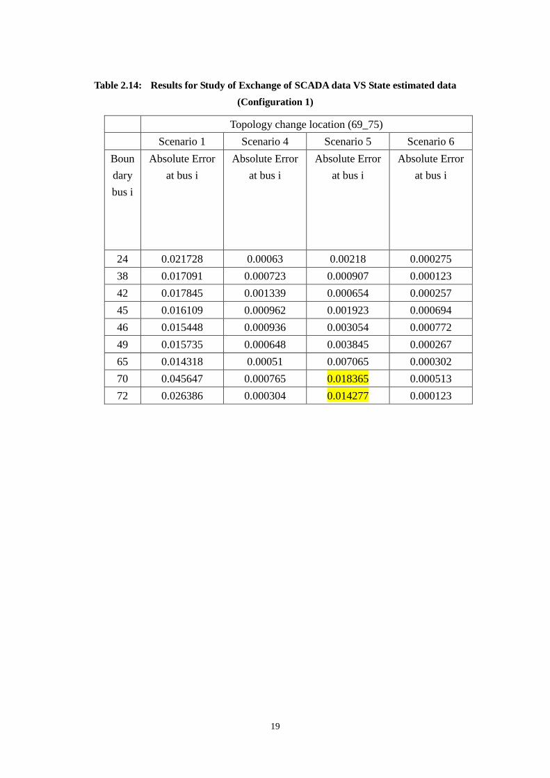
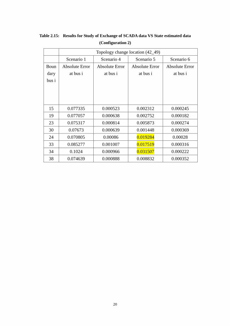
The results of the simulation are shown in Tables 2.12 to 2.16 below. It is noted

that for these experiments, the errors of the boundary buses (both internal and external) are observed, since it is anticipated that for this study, the errors will be most prominent at these locations. For all cases, it is observed that the solutions obtained for SCADA data exchange and up-to-date SE data exchange are basically identical, and same as the exact solution. This is reasonable, since those two scenarios basically represent situations where the data exchanged is ideal and correct, and intuitively, this means the state estimation solutions should also be correct.

However, large errors may appear at boundary buses in the event where the state estimated data obtained from Area 2 in step (i) is not up-to-date. Some cases with topology changes where this can be observed are shown in Tables 2.12 to 2.16, with the buses incurring large errors being highlighted.

17

Table 2.12: Results for Study of Exchange of SCADA data VS State estimated data (Configuration 1)

Topology change location (49_66) Scenario 1 Scenario 4 Scenario 5 Scenario 6

Boundary bus i

Absolute Error at bus i




24 0.01129 0.000655 0.000648 0.000128 38 0.017443 0.000739 0.007645 1.67E-05 42 0.035787 0.00093 0.013582 0.000133 45 0.067575 0.000502 0.018416 0.00084 46 0.076709 0.000529 0.035493 0.000809 49 0.11679 0.000203 0.060025 0.000258 65 0.058791 0.000605 0.064716 0.000167 70 0.004671 0.001006 0.008073 0.000596 72 0.007141 0.00041 0.006352 0.000184

18



Boundary bus i





24 0.043033 0.000339 0.005348 1.90E-05 38 0.031355 0.000499 0.002411 0.000183 42 0.03275 0.00121 0.001778 0.000218 45 0.031349 0.001023 0.003083 7.57E-05 46 0.030678 0.001001 0.005698 0.00026 49 0.030875 0.0007 0.008358 0.000112 65 0.023844 0.000602 0.020869 0.000354 70 0.10507 0.000658 0.046367 0.000361 72 0.05593 0.001023 0.037634 0.0001

19



Boundary bus i





24 0.021728 0.00063 0.00218 0.000275 38 0.017091 0.000723 0.000907 0.000123 42 0.017845 0.001339 0.000654 0.000257 45 0.016109 0.000962 0.001923 0.000694 46 0.015448 0.000936 0.003054 0.000772 49 0.015735 0.000648 0.003845 0.000267 65 0.014318 0.00051 0.007065 0.000302 70 0.045647 0.000765 0.018365 0.000513 72 0.026386 0.000304 0.014277 0.000123

20



Boundary bus i





15 0.077335 0.000523 0.002312 0.000245 19 0.077057 0.000638 0.002752 0.000182 23 0.075317 0.000814 0.005873 0.000274 30 0.07673 0.000639 0.001448 0.000369 24 0.070805 0.00086 0.019284 0.00028 33 0.085277 0.001007 0.017519 0.000316 34 0.1024 0.000966 0.031507 0.000222 38 0.074639 0.000888 0.008832 0.000352

21



Boundary bus i





15 0.046478 0.000418 0.001708 0.000354 19 0.046211 0.000467 0.00182 0.000306 23 0.052342 0.000696 0.006521 5.76E-05 30 0.046701 0.000408 0.002284 0.0002 24 0.057723 0.00083 0.020064 0.000154 33 0.047223 0.000914 0.006797 0.000353 34 0.047855 0.000686 0.01298 0.000244 38 0.04207 0.00054 0.011912 0.000153

In the above tables, locations where the errors at boundary buses are large even

with some level or type of data exchange are highlighted. It can be observed that exchanging state estimated data which is not updated in time may lead to large boundary bus errors in ensuing state estimator solutions. However, this should not be a serious issue since the state estimated data which is exchanged would be updated to reflect topological knowledge is more important to the accuracy of state estimators.

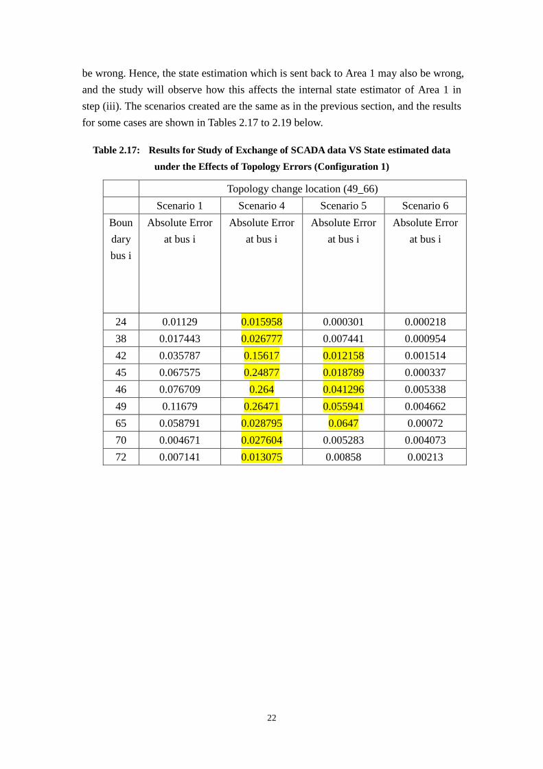
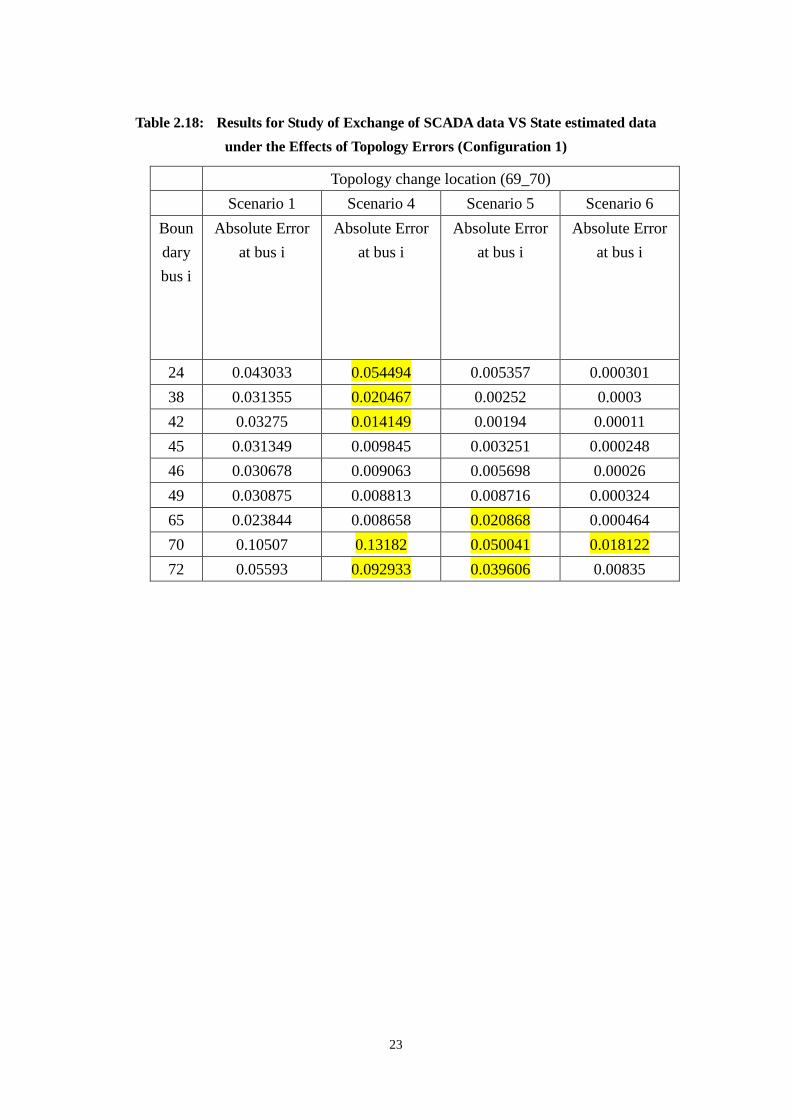
The results in the previous part confirm the belief that exchanging either up to date SE data or SCADA data give near identical state estimation results. In this part, the effects of topology errors in the external system’s topology processor will be investigated. For this part of the investigation, the topology processor assumes the base case topology even when there is a line outage, meaning that the topology change cannot be seen. For scenarios involving SCADA data exchange, this means that the internal state estimator will use updated analog measurements for all buses in the system, but the state estimator will be run using the wrong system topology. For scenarios involving SE data exchange, this implies that in step (ii) of the process, Area 2 will be using updated measurements in its own area, together with Area 1’s state estimated data, but the topology data which is used during state estimation will also

22

be wrong. Hence, the state estimation which is sent back to Area 1 may also be wrong, and the study will observe how this affects the internal state estimator of Area 1 in step (iii). The scenarios created are the same as in the previous section, and the results for some cases are shown in Tables 2.17 to 2.19 below.

Table 2.17: Results for Study of Exchange of SCADA data VS State estimated data under the Effects of Topology Errors (Configuration 1)


Boundary bus i





24 0.01129 0.015958 0.000301 0.000218 38 0.017443 0.026777 0.007441 0.000954 42 0.035787 0.15617 0.012158 0.001514 45 0.067575 0.24877 0.018789 0.000337 46 0.076709 0.264 0.041296 0.005338 49 0.11679 0.26471 0.055941 0.004662 65 0.058791 0.028795 0.0647 0.00072 70 0.004671 0.027604 0.005283 0.004073 72 0.007141 0.013075 0.00858 0.00213

23



Boundary bus i





24 0.043033 0.054494 0.005357 0.000301 38 0.031355 0.020467 0.00252 0.0003 42 0.03275 0.014149 0.00194 0.00011 45 0.031349 0.009845 0.003251 0.000248 46 0.030678 0.009063 0.005698 0.00026 49 0.030875 0.008813 0.008716 0.000324 65 0.023844 0.008658 0.020868 0.000464 70 0.10507 0.13182 0.050041 0.018122 72 0.05593 0.092933 0.039606 0.00835

24



Boundary bus i





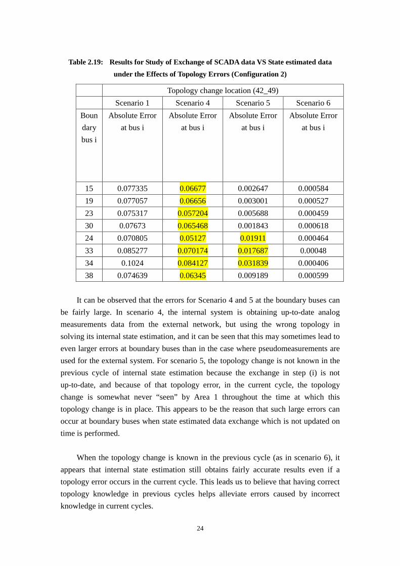
15 0.077335 0.06677 0.002647 0.000584 19 0.077057 0.06656 0.003001 0.000527 23 0.075317 0.057204 0.005688 0.000459 30 0.07673 0.065468 0.001843 0.000618 24 0.070805 0.05127 0.01911 0.000464 33 0.085277 0.070174 0.017687 0.00048 34 0.1024 0.084127 0.031839 0.000406 38 0.074639 0.06345 0.009189 0.000599

It can be observed that the errors for Scenario 4 and 5 at the boundary buses can

be fairly large. In scenario 4, the internal system is obtaining up-to-date analog measurements data from the external network, but using the wrong topology in solving its internal state estimation, and it can be seen that this may sometimes lead to even larger errors at boundary buses than in the case where pseudomeasurements are used for the external system. For scenario 5, the topology change is not known in the previous cycle of internal state estimation because the exchange in step (i) is not up-to-date, and because of that topology error, in the current cycle, the topology change is somewhat never “seen” by Area 1 throughout the time at which this topology change is in place. This appears to be the reason that such large errors can occur at boundary buses when state estimated data exchange which is not updated on time is performed.

When the topology change is known in the previous cycle (as in scenario 6), it appears that internal state estimation still obtains fairly accurate results even if a topology error occurs in the current cycle. This leads us to believe that having correct topology knowledge in previous cycles helps alleviate errors caused by incorrect knowledge in current cycles.

25

As aforementioned, the measurements used for state estimation in the

experiments are created through incorporating small errors in the power flow solutions, and up to this part, the errors have always been bounded by ±0.01 p.u. Now, the errors are increased and bounded by ±0.05 p.u. and the experiments to investigate the differences between exchanging SCADA and state estimated data are repeated. It is important to note that all values used in the state estimator programs are in per unit already.

As the errors are increased, the accuracy of the state estimator decreases slightly for all scenarios as expected, but the extent of the drop in accuracy is not substantial. Moreover, the decrease in accuracy is noted for all scenarios, so there is no evidence suggesting that exchanging state estimated data is more beneficial than exchanging SCADA data, or vice versa for situations where the measurement devices are less accurate and have greater noise.

2.4 Summary

In this chapter, studies have been performed to study the effects of different levels and types of data exchange with the external system on the accuracy of internal state estimation. Simulation results show that having data exchange with the external system helps improve internal system state estimation accuracy, especially in situations where there are large changes in the operating conditions of the system, such as during topology changes in the external system. Further studies on levels of data exchange also show that correct knowledge of topology is more influential than knowledge of analog measurements in ensuring a high level of accuracy for internal system state estimation.

Finally, the effects of exchanging SCADA data versus state estimated data are also studied. It is observed that exchanging state estimated data which is not up to date can lead to some errors at boundary buses in ensuing state estimations. It is also noted that exchanging SCADA data when there are topology errors leads to very large errors at boundary buses, while exchanging state estimated data alleviates this issue slightly as long as there is correct information of topology in preceding sets of data exchange.

26

3 Impact of external system measurements on internal state estimation

3.1 Introduction

This section investigates the use of a few real-time measurements (conventional as well as synchronized phasor measurements) from the external system. The first part is concerned about the impact of these measurements on the state estimation solution for the internal system as well as on the results of contingency analysis. The second part investigates the optimal selection of these measurements in order to maximize their benefits. A brief overview of both of these parts will be given below, before providing their detailed descriptions and results. a) Impact of external system measurements on internal state estimation

Monitoring of a power system involves measurements which must be sufficient

to observe the entire system state. When operating a large interconnected system, each utility has detailed information about its own system, while having limited access to the measurements from its neighboring systems, which are collectively referred as the “external” system. This lack of real-time information both of the measurements as well as the network model constitutes the single most important source of errors in subsequent contingency analysis that is conducted by each utility control center. Incorrect modeling of the external system will lead to errors that might be unacceptably high under certain operating conditions. Hence, an improvement in the way external systems are monitored will have a significant impact on the operation of interconnected power systems.

Recent increase in the number of synchronized phasor measurements installed in various substations in power systems provides an opportunity for making such an improvement. Synchronized phasor measurements are typically available via the phasor data concentrators which provide time tags and therefore allow system-wide measurement data to be available at local control centers. State estimators can take advantage of the availability of synchronized phasor measurements from the external system in order to improve the external network’s estimated state and network model. As a result, reliability and accuracy of the subsequent calculations involving system security such as the contingency analysis can be significantly improved. While phasor measurement units (PMU) are rapidly populating power systems, their numbers are still low to allow observability of systems based exclusively on PMU measurements. Thus, it is worth investigating the incremental benefits to be gained by taking

27

advantage of their limited presence in the external system. Section 3.2 studies this problem by simulating scenarios where the operating conditions, location and number of available PMU measurements as well as the network model change for a given test system and its neighbors, i.e. its external system. IEEE 118 bus system is used for this purpose by designating a subset of buses as the internal and the remaining buses as the external system buses.

Those buses in the external system having direct connections to the internal system are defined as the boundary buses. It is noted that the internal system buses plus the boundary buses typically constitute a single observable island based on the internal system real-time measurements. Hence, those measurements used for the external system are either pseudo-measurements provided by the load forecasting and/or generation scheduler functions or they may seldom contain actual real-time measurements received through inter-utility real-time measurement exchange. In either case, due to the lack of redundancy, their impact on the internal state estimation will be minimal or null. On the other hand, they will have a very significant impact on the contingency analysis associated with the internal system topology changes due to their effect in building the external network model.

The objective of the first part of this study is to highlight the role which few available PMU measurements might play in improving the external network model. Specifically, section 3.2 investigates the role of the location, number and type of these measurements in an attempt to develop guidelines and strategies to optimally place them when a limited number of them are available for placement.

The problem is formulated using an external equivalent, which is obtained by first converting all external bus injections into equivalent shunt branches and then applying Kron reduction to the external system buses. This equivalent will be accurate as long as the load and topology of the system remains constant. The objective of the study is to show the impact of a few real-time external measurements (provided by PMUs) on the internal state estimation solution. PMUs are assigned to three different subsets of external system buses, and the impact of these real-time measurements on internal state estimation solution as well as on the subsequent contingency analysis is investigated by changing the system loading. b) Optimal selection of external system measurements

28

Using the static Kron equivalent to model the external system, will lead to inaccuracies as the operating conditions change during the daily operation. Manifestation of these inaccuracies and their impact on internal state estimation solution and contingency analysis are illustrated in section 3.2. However, no recommendation is made about the optimal placement of the PMUs in the external system. Section 3.3 presents the results of a study that aims to identify the optimal set of external system measurements which will have the most significant impact on internal state estimation.

It is assumed that enough measurements are available to make the internal system fully observable. The objective of this part of the study is to identify the number and location of those external measurements whose exchange will improve the internal state estimation the most. Several previous studies illustrate the impact a transmission line outage in the external system on internal system power flow solution [9]-[13]. Sensitivity based selection of buffer areas to improve the performance of the equivalents is investigated in [14]-[21].

In this project, in determining the optimal subset of external system measurements, both line flow and power injection measurements are considered as candidates. The problem is formulated using the sensitivity of the internal system estimated states to the external system measurements, as a criterion to be maximized. However, since the sensitivity of the state estimation solution is a linear combination of all the external system measurements, their cumulative effect is to be considered. This is accomplished by formulating the problem as an linear mixed integer programming problem where the selected set of external system measurements will yield the smallest error between the true and equivalence solutions. Since it is an approximation, the desired error tolerance can be specified by the system operator.

3.2 Effect of Using External System Synchronized Phasor Measurements on Internal System State Estimation Solution

3.2.1 Problem Formulation

3.2.1.1 Transforming power injections at external buses

The net current injection at a substation is zero if there is no load and generation at that substation. Voltages of buses with zero injections can be eliminated from the system of equations in order to obtain the reduced equivalent network model.

29

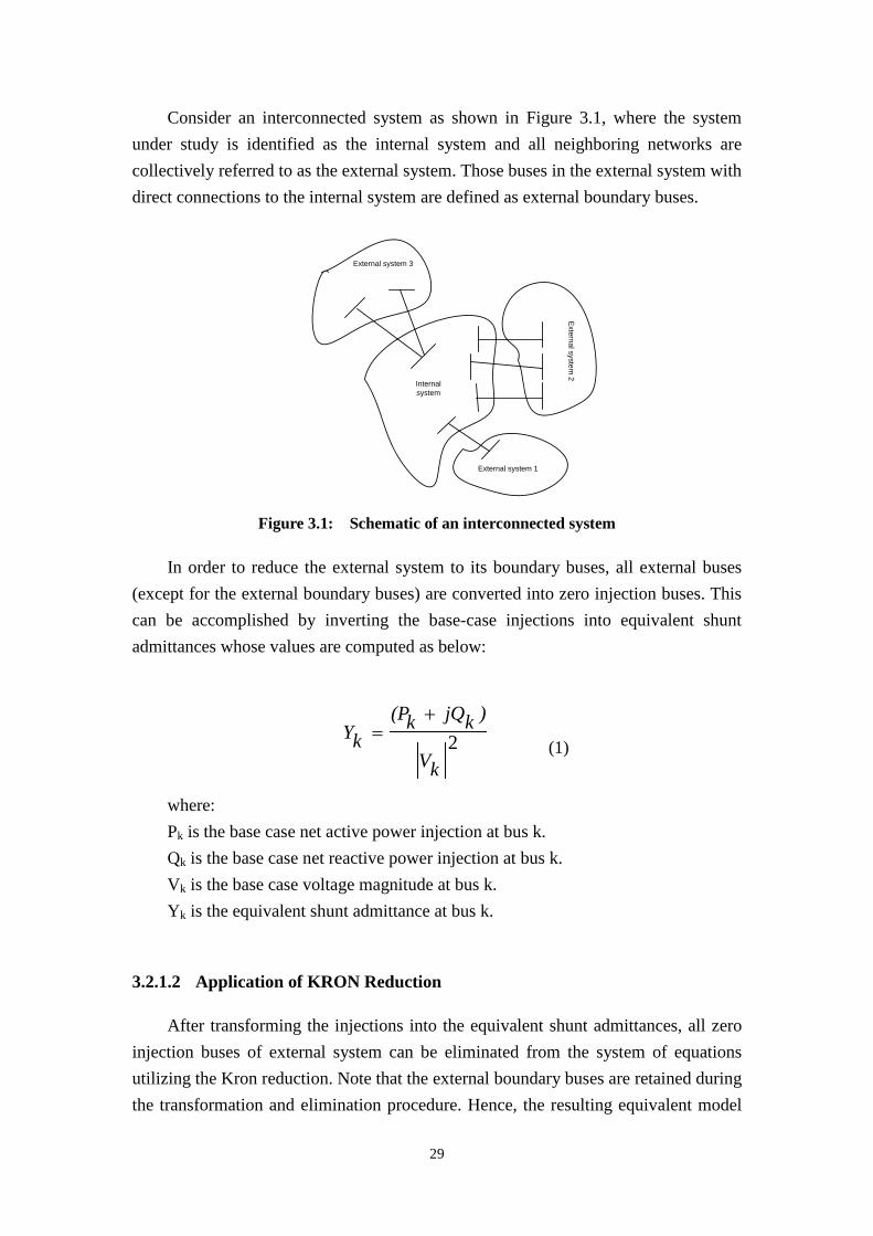
Consider an interconnected system as shown in Figure 3.1, where the system under study is identified as the internal system and all neighboring networks are collectively referred to as the external system. Those buses in the external system with direct connections to the internal system are defined as external boundary buses.

Internal system

External system 3

External system

2

External system 1

Figure 3.1: Schematic of an interconnected system

In order to reduce the external system to its boundary buses, all external buses (except for the external boundary buses) are converted into zero injection buses. This can be accomplished by inverting the base-case injections into equivalent shunt admittances whose values are computed as below:

2kV

)kjQk(PkY

+=

(1)

where: Pk is the base case net active power injection at bus k. Qk is the base case net reactive power injection at bus k. Vk is the base case voltage magnitude at bus k. Yk is the equivalent shunt admittance at bus k.

3.2.1.2 Application of KRON Reduction

After transforming the injections into the equivalent shunt admittances, all zero injection buses of external system can be eliminated from the system of equations utilizing the Kron reduction. Note that the external boundary buses are retained during the transformation and elimination procedure. Hence, the resulting equivalent model

30

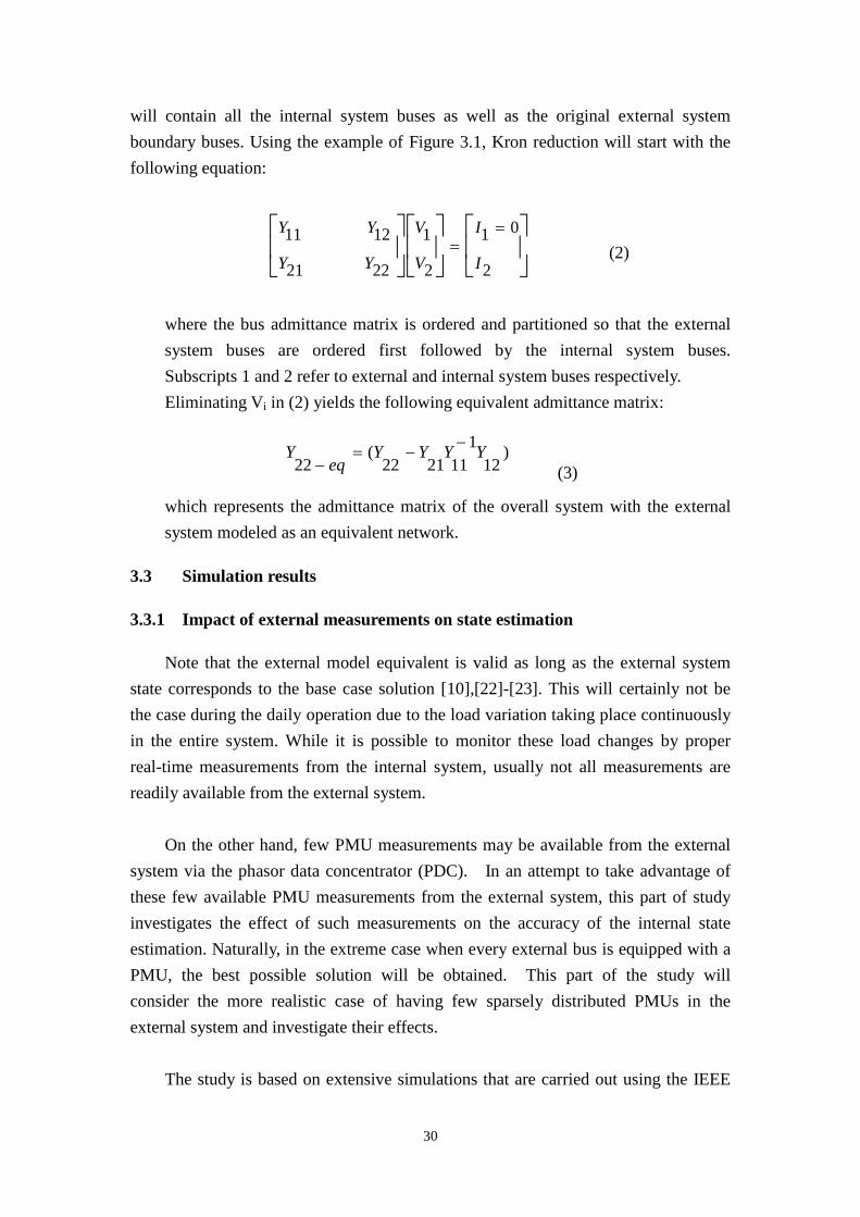
will contain all the internal system buses as well as the original external system boundary buses. Using the example of Figure 3.1, Kron reduction will start with the following equation:

==

2

01

2

1

2221

1211

I

I

V

V

YY

YY (2)

where the bus admittance matrix is ordered and partitioned so that the external system buses are ordered first followed by the internal system buses. Subscripts 1 and 2 refer to external and internal system buses respectively. Eliminating Vi in (2) yields the following equivalent admittance matrix:

)12

1112122

(22

YYYYeq

Y −−=−

(3)

which represents the admittance matrix of the overall system with the external system modeled as an equivalent network.

3.3 Simulation results

3.3.1 Impact of external measurements on state estimation

Note that the external model equivalent is valid as long as the external system state corresponds to the base case solution [10],[22]-[23]. This will certainly not be the case during the daily operation due to the load variation taking place continuously in the entire system. While it is possible to monitor these load changes by proper real-time measurements from the internal system, usually not all measurements are readily available from the external system.

On the other hand, few PMU measurements may be available from the external system via the phasor data concentrator (PDC). In an attempt to take advantage of these few available PMU measurements from the external system, this part of study investigates the effect of such measurements on the accuracy of the internal state estimation. Naturally, in the extreme case when every external bus is equipped with a PMU, the best possible solution will be obtained. This part of the study will consider the more realistic case of having few sparsely distributed PMUs in the external system and investigate their effects.

The study is based on extensive simulations that are carried out using the IEEE

31

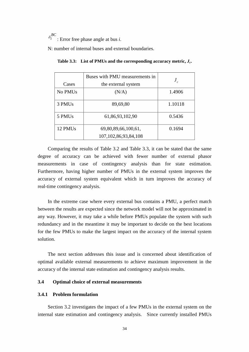
118-bus system as an example. The system is partitioned into subsystems representing the internal and external systems. Buses belonging to internal and external systems and their boundaries are listed in Table 3.1.

Several external system equivalents are developed by considering different number of buses with PMU measurements in the external system. All the equivalents are developed using base case loading conditions. In developing these equivalents, in addition to the external boundary buses, those buses with assumed PMU measurements are retained as well.

Changes in system loads are simulated by increasing all loads and generation by 10%. A power flow solution for the entire system is obtained corresponding to this new loading. This solution will subsequently be used as the “perfect” reference in evaluating the accuracy of the internal system state estimation obtained by using different external network equivalents.

Table 3.1: 118-Bus Example: Internal and External System Buses

Internal system

Internal Boundary

External System

External Boundary

1,2,3,4,5,6,7,8,9,10, 11,12,13,14,15,16, 17,18,19,20,21,22, 23,24,25,26,27,28, 29,30,31,32,33,34, 35,36,37,38,39,40, 41,42,43,44,45,113, 114,115,117

24,38,42,45 47,48,50,51,52,53,54, 55,56,57,58,59,60,61, 62,63,64,66,67,68,69, 71,73,74,75,76,77,78, 79,80,81,82,83,84,85, 86,87,88,89,90,91,92, 93,94,95,96,97,98,99, 100,101,102,103,104, 105,106,107,108,109, 110,111,112,116,118.

46,49,65,70,72

In using the equivalents that contain PMU buses, synchronized phasor

measurements are taken from the perfect reference solution, representing the correct real-time measurements which will be available via the GPS system. However, network equivalent branch parameters will have errors due to the fact that they correspond to the base case loading conditions.

Table 3.2 shows the results of state estimation using the internal system and the

32

external network equivalent for different cases where different numbers of PMU buses are retained while obtaining the external system equivalent. The following accuracy metric will be used to compare the improvement in the accuracy of the estimated state for different cases considered:

−+

−=

2)ˆ(

2)ˆ(1

PFi

BCii

BCiV

BCiViV

NJ

δ

δδ (4)

N: number of the buses

iV : Estimated voltage magnitude for bus i.

BCiV : Error free voltage magnitude at bus i.

iδ : Estimated phase angle at bus i.

BCiδ : Error free phase angle at bus i.

It is evident from Table 3.2 that the error criterion J is improved as the number of

retained buses with PMU measurements in the external system is gradually increased.

Table 3.2: List of PMUs and the corresponding accuracy metric, J.

Cases

Buses with PMU measurements in the external system

J

No PMUs (N/A) 0.0071

4 PMUs 83,94,103,111 0.0053

5 PMUs 79,88,92,104,109 0.0043

20 PMUs 48,69,73,74,76,78,96,93,80,116,67,60, 53,51,57,108,104,102,90,86

0.0022

3.3.2 Effect of PMUs on real-time contingency analysis

While the effect of PMUs on internal system state estimation appears significant, this can be minimized or even completely eliminated by properly choosing the measurement set corresponding to the external system. This set can be chosen as a

33

strictly critical set, making their effect on the internal system null, in other words making them dormant measurements [9]. However, this will not be of much use for real-time contingency analysis which requires an accurate real-time external network model for accurate prediction of possible security violations.

Every control center identifies a list of important contingencies which are periodically analyzed in order to maintain static system security. Obtaining an accurate contingency analysis result greatly depends on the accuracy of the external network model. Hence, in addition to the internal system state, the state estimator should provide a good approximation of the external network model. This can be accomplished by first obtaining a state estimation solution that uses all available external system PMU measurements and then calculating the estimated values of the external system bus injections using this solution. Estimated external system bus injections along with the network model will then be used for subsequent contingency analysis. The location and number of PMU measurements used for this purpose will have an impact on the accuracy of contingency analysis results. In this study, only branch outage type contingencies are considered for the internal system.

The above described procedure can be illustrated by the following example. Consider the outage of line 26-30 which is in the internal system, as the contingency of interest. Different numbers of PMUs will be considered to be installed in the external system. A state estimation solution followed by contingency analysis will be executed for each of these cases. Table 3.3 shows a list of PMU locations and their impact on internal system contingency analysis. The accuracy of contingency analysis will be evaluated using a metric similar to the one defined earlier. The correct power flow solution for the entire interconnected system with increased loading and line 26-30 outage is calculated and saved as the “reference” solution. Then, the accuracy metric is defined as follows:

∑

−+−=N

i

BCii

BCiViVJ 2)ˆ(2)ˆ( δδ (5)

where:

iV : Estimated voltage magnitude for bus i.

BCiV : Error free voltage magnitude at bus i.

iδ : Estimated phase angle at bus i.

34

BCiδ : Error free phase angle at bus i.

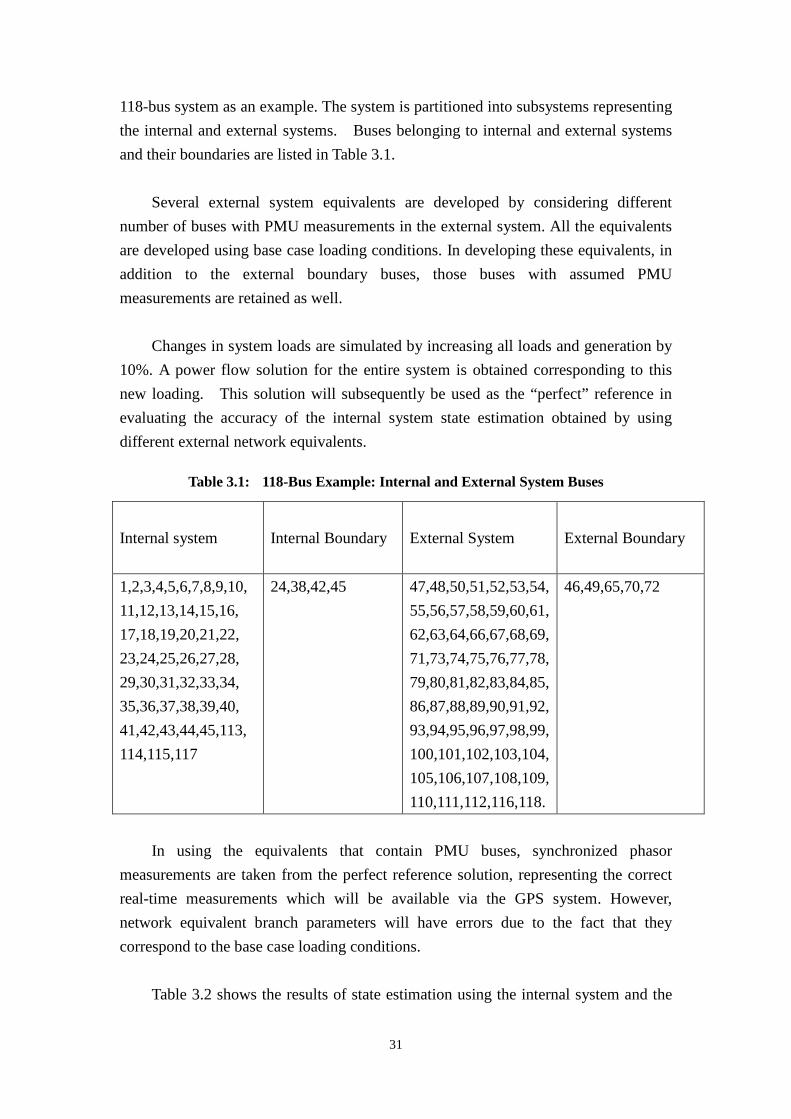
N: number of internal buses and external boundaries.

Table 3.3: List of PMUs and the corresponding accuracy metric, Jc.

Comparing the results of Table 3.2 and Table 3.3, it can be stated that the same degree of accuracy can be achieved with fewer number of external phasor measurements in case of contingency analysis than for state estimation. Furthermore, having higher number of PMUs in the external system improves the accuracy of external system equivalent which in turn improves the accuracy of real-time contingency analysis.

In the extreme case where every external bus contains a PMU, a perfect match between the results are expected since the network model will not be approximated in any way. However, it may take a while before PMUs populate the system with such redundancy and in the meantime it may be important to decide on the best locations for the few PMUs to make the largest impact on the accuracy of the internal system solution.

The next section addresses this issue and is concerned about identification of optimal available external measurements to achieve maximum improvement in the accuracy of the internal state estimation and contingency analysis results.

3.4 Optimal choice of external measurements

3.4.1 Problem formulation

Section 3.2 investigates the impact of a few PMUs in the external system on the internal state estimation and contingency analysis. Since currently installed PMUs

Cases

Buses with PMU measurements in the external system cJ

No PMUs (N/A) 1.4906

3 PMUs 89,69,80 1.10118

5 PMUs 61,86,93,102,90 0.5436

12 PMUs 69,80,89,66,100,61, 107,102,86,93,84,108

0.1694

35

are not very many, it is logical to also consider the use of real-time conventional measurements from the external system. These will be the measurements whose real-time updates will bring the most benefits to the internal system state estimation and the subsequent contingency analysis.

This part of study formulates the external system measurement selection as a mixed integer programming problem whose objective is to minimize the number of such measurements while maintaining a pre-defined accuracy level for the internal system solution. This is accomplished by first developing the sensitivity matrix of the internal system state estimates to the external system measurements. This is followed by formulation of the optimization problem in order to identify the optimal set of external system measurements to be exchanged in real time. The procedure is applied to IEEE 118 bus system as an illustration and experimental verification.

3.4.1.1 Sensitivity matrix

It is well documented that the solution of the state estimation problem depends not only on the internal system model and measurements but on the representation of the external system and its measurements as well. Consider an interconnected system as shown in Figure 3.1, where the part designated as the internal system represents the area of interest and its neighboring systems are shown as external systems 1 through 3. Those buses that belong to external systems but have direct connections to the internal system will be referred as “external boundary” buses.

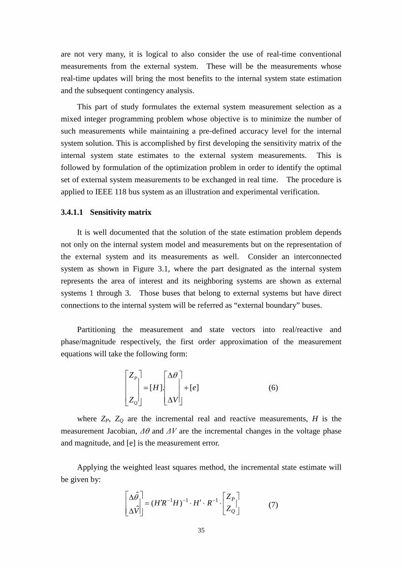
Partitioning the measurement and state vectors into real/reactive and phase/magnitude respectively, the first order approximation of the measurement equations will take the following form:

][].[ eV

HZ

Z

Q

P

+

∆

∆=

θ

(6)

where ZP, ZQ are the incremental real and reactive measurements, H is the measurement Jacobian, Δθ and ΔV are the incremental changes in the voltage phase and magnitude, and [e] is the measurement error.

Applying the weighted least squares method, the incremental state estimate will be given by:

⋅⋅′⋅′=

∆

∆ −−−

Q

P

ZZ

RHHRHV

111 )(ˆθ

(7)

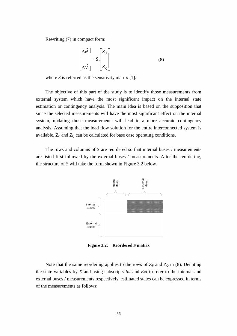
36

Rewriting (7) in compact form:

=

∆

∆

Q

P

Z

ZS

V

.ˆ

θ

(8)

where S is referred as the sensitivity matrix [1].

The objective of this part of the study is to identify those measurements from external system which have the most significant impact on the internal state estimation or contingency analysis. The main idea is based on the supposition that since the selected measurements will have the most significant effect on the internal system, updating those measurements will lead to a more accurate contingency analysis. Assuming that the load flow solution for the entire interconnected system is available, ZP and ZQ can be calculated for base case operating conditions.

The rows and columns of S are reordered so that internal buses / measurements are listed first followed by the external buses / measurements. After the reordering, the structure of S will take the form shown in Figure 3.2 below.

Exte

rnal

M

eas.

Internal Buses

External Buses

Inte

rnal

M

eas.

Figure 3.2: Reordered S matrix

Note that the same reordering applies to the rows of ZP and ZQ in (8). Denoting

the state variables by X and using subscripts Int and Ext to refer to the internal and external buses / measurements respectively, estimated states can be expressed in terms of the measurements as follows:

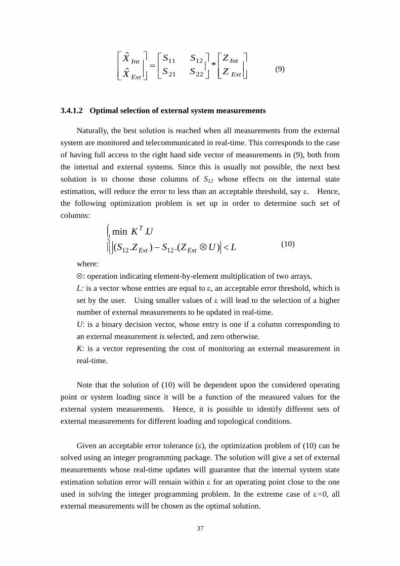
37

=

Ext

Int

Ext

Int

ZZ

SSSS

X

X*

ˆ

ˆ

2221

1211

(9)

3.4.1.2 Optimal selection of external system measurements

Naturally, the best solution is reached when all measurements from the external system are monitored and telecommunicated in real-time. This corresponds to the case of having full access to the right hand side vector of measurements in (9), both from the internal and external systems. Since this is usually not possible, the next best solution is to choose those columns of S12 whose effects on the internal state estimation, will reduce the error to less than an acceptable threshold, say ε. Hence, the following optimization problem is set up in order to determine such set of columns:

<⊗− LUZSZSUK

ExtExt

T

).().(.min

1212

(10)

where: ⊗: operation indicating element-by-element multiplication of two arrays. L: is a vector whose entries are equal to ε, an acceptable error threshold, which is set by the user. Using smaller values of ε will lead to the selection of a higher number of external measurements to be updated in real-time. U: is a binary decision vector, whose entry is one if a column corresponding to an external measurement is selected, and zero otherwise. K: is a vector representing the cost of monitoring an external measurement in real-time.

Note that the solution of (10) will be dependent upon the considered operating

point or system loading since it will be a function of the measured values for the external system measurements. Hence, it is possible to identify different sets of external measurements for different loading and topological conditions.

Given an acceptable error tolerance (ε), the optimization problem of (10) can be solved using an integer programming package. The solution will give a set of external measurements whose real-time updates will guarantee that the internal system state estimation solution error will remain within ε for an operating point close to the one used in solving the integer programming problem. In the extreme case of ε=0, all external measurements will be chosen as the optimal solution.

38

Once a solution is obtained, simulations are used to validate the chosen set of

external measurements, both for internal state estimation as well as for subsequent contingency studies. The following procedure is carried out for this purpose:

Obtain power flow solutions for the entire system both for base case as well as 20% above base case loading conditions.

1. For a given accuracy tolerance ε, solve the integer programming problem of (10).

Obtain the solution U, which identifies those external measurements to be updated in real-time.

2. Consider the power flow case corresponding to the loading conditions 20% above base case. Update all internal measurements and those from external which have been identified in step 1, keep the rest of external measurements at their base case power flow solution values.

3. Estimate the system state and all injections at external system buses. 4. Run contingency analysis for the internal system using the network model

estimated in step 3. Compare the results with the exact solution which can be obtained using the entire system model with exact model. The corresponding flow chart is shown in Figure 3.3.

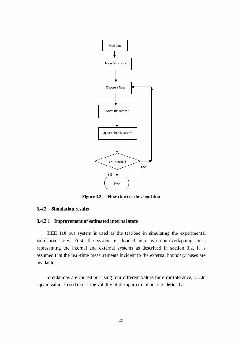
39

Figure 3.3: Flow chart of the algorithm

3.4.2 Simulation results

3.4.2.1 Improvement of estimated internal state

IEEE 118 bus system is used as the test-bed in simulating the experimental validation cases. First, the system is divided into two non-overlapping areas representing the internal and external systems as described in section 3.2. It is assumed that the real-time measurements incident to the external boundary buses are available.

Simulations are carried out using four different values for error tolerance, ε. Chi square value is used to test the validity of the approximation. It is defined as:

Read Data

Form Sensitivity

Choose a New

Solve the Integer

Update the Chi square

J < Threshold

Stop

No

YES

40

∑=

′−′=

n

i iiR

iZiZJ

1

2))(1ˆ)(1(

(11)

where: n is the number of internal measurements.

1Z ′ , is the internal system measurement vector.

1Z ′ , is the internal system estimated measurement.

iiR is the ith diagonal entry of error covariance matrix. Table 3.4 shows the chi square values for different choices of accuracy tolerance

ε.

Table 3.4: Chi square values for different choices of accuracy tolerance ε.

Accuracy Tolerance

(ε)

Number of selected measurements

Chi-square value (J)

0.01 24 out of 166 18637.14

1e-4 61 out of 166 3462.20

1e-5 69 out of 166 3.453

1e-35 166 out of 166 0.521

Using the chi squares test as the cut-off criteria, in this case study ε = 1e-5 is

determined as the acceptable cut-off value. Note the sudden drop in Chi Square value when the error threshold is changed from 10-4 to 10-5. The chi square value corresponding to the latter is not statistically significant according to chi squares distribution, implying that the selection of 69 measurements will be sufficient to maintain an internal solution with acceptable accuracy at ε level.

Since the true state is known via the power flow result, the degree of approximation in the estimated state with respect to this true value can also be calculated as an alternative metric as given below:

))ˆ

()ˆ

((1 2

1

2refi

irefi

n

iref

i

iref

i

VVV

n θ

θθρ

−+

−= ∑

= (12)

41

where: n is the number of internal buses.

refiV : is the true solution for voltage of bus i.

refiθ is the true angle of bus i.

iV is the estimated voltage for bus i.

iθ is the estimated angle for bus i.

Table 3.5 shows the results of using the error metric defined in (12).

Table 3.5: Error Metric of (12)

Accuracy Tolerance (ε)


ρ

10 0 out of 166 0.1291 0.01 24 out of 166 0.01358

1.0 e-4 61 out of 166 3.89 e-4 1.0 e-5 69 out of 166 2.04 e-6

3.4.2.2 Impact of online external measurement exchange on contingency analysis

Performance of the estimated external system model based on the limited number of real-time updated measurements can also be tested by considering the contingency analysis. In this case, the external system model will be built using the state estimation results that are obtained based on the full internal and selected external measurement set. This model will then be used to solve the power flow problem where a contingency will be applied to the internal system. In this study, only line outage type contingencies are considered.

Consider the contingency where one of the main transmission lines of in the internal system (line 26-30) is taken out of service. The true solution corresponding to this contingency can be obtained by solving the entire system with proper topology change. This solution can then be compared with the one obtained using the model

42

based on limited external system measurements. An error metric similar to the one in (12) can be defined as follows:

))()((1 2

1

2refi

upi

refi

n

iref

i

upi

refi

VVV

n θ

θθβ

−+

−= ∑

= (13)

where: n is the number of internal buses.

refiV : is the true solution for voltage of bus i.

refiθ is the true angle of bus i.

upiV is the power flow solution for voltage of bus i, using the updated

measurements.

upiθ is the power flow solution for angle of bus i, using the updated

measurements.

Table 3.6 shows the computed metric of (13) for different error tolerance limits corresponding to the line 26-30 outage contingency.

Table 3.6: Error metric of (13) for contingency case

In order to apply the method for a large interconnected network, the proposed

method should be repeated for different operating conditions. Solution of the optimization problem for different operating conditions yields different sets of optimal external measurements to be exchanged in real-time. This suggests that based on the load forecasting and available seasonal load characteristic, the proposed method would have to be repeatedly applied for different loading conditions.

The practical implementation may take different forms depending upon the load and switching characteristics of the specific power system. If significant differences

Accuracy Tolerance (ε)


β

10 0 out of 166 0.2698 0.01 24 out of 166 0.00694

1.0 e-4 61 out of 166 0.000689 1.0 e-5 69 out of 166 0.000579

43

are observed during daily load cycles, then the method can be repeated several times daily. Alternatively, it can be repeated less frequently only to account for seasonal load variations.

3.5 Conclusions

This chapter presents the results of two studies undertaken in this project. The first part of chapter studies the impact of receiving limited number of real time PMU measurements from the external system on the accuracy of the internal system state estimation and contingency analysis results. Simulation results clearly illustrate benefits gained by using more PMUs in the external system. The second part of the chapter considers the case where a limited number of external system conventional measurements can be telemetered in real-time. It develops an optimal selection approach for a minimum number of such measurements so that a pre-defined error metric for the internal system solution will be minimized.

Due to lack of availability of real data from utility company, methods are tested on IEEE 118 bus system where system is split into two subsystems: representing internal and external systems.

44

4 Conclusions

Hierarchical and distributed state estimators have been studied mainly from an algorithmic solution viewpoint, and there have not been studies on the factors regarding the actual implementation of a hierarchical and distributed SE. In this project, the effects of different types and levels of data exchange on internal state estimation are studied on the IEEE 118 bus system.

In the preliminary study, the detailed external model is adopted. As expected, the implementation of data exchange with neighboring areas helps improve the accuracy of internal state estimation, with the improvement being more significant when there are large changes in the system operating conditions. Further investigation is then performed to investigate the effects of exchanging data with only certain parts of the external system. Simulation results illustrate that incorrect knowledge of topology data plays a major role in causing the accuracy of internal state estimation to deteriorate.

Studies are also performed to compare the exchange of SCADA data versus state estimated data on internal state estimation accuracy. Results illustrate that exchanging SCADA data and state estimated data are the same in the case where the data exchanged is up to date. However, exchange of SCADA data in the event when there are errors in topology can lead to very large errors in internal state estimation. It is worth noting that this problem is alleviated when state estimated data is exchanged if there are previous sets of data with correct topology data.

Another objective of this project is in studying the effects of incorporating PMUs in the external system on internal state estimation accuracy. This part focuses on changes in load, with the external system model created based on the amount of PMUs to be incorporated. Results illustrate that the inclusion of PMUs from the external system helps improve the accuracy of internal state estimation. Furthermore, the effects of incorporating PMUs in the external model on improvement of contingency analysis are also studied and simulations show that the improvement in contingency analysis is more pronounced with an increasing number of PMUs.

Finally, an algorithm to determine the optimal selection of conventional measurements in the external system to improve internal state estimation is also provided. Based on different system operating conditions, the selection of measurements would be different, and hence, the external model as well. Simulations

45

illustrate that the optimal selection approach can minimize the number of measurements required to minimize a predefined error metric for internal state estimation.

46

References

[1] Metrics for Determining the Impact of Phasor Measurements on Power System State Estimation, Eastern Interconnection Phasor Project, March 2006.

[2] A. Abur and A. G. Exposito, Power System State Estimation: Theory and Implementation, Marcel Dekker Inc., 2004.

[3] Th. Van Cutsem, J. L. Howard, M. Ribben-Pavalla, Y.M. El-Fattah, “Hierarchical State Estimation”, International Journal of Electric Power and Energy Systems, Vol. 2, pp.70-81, April 1980.

[4] Th. Van Cutsem, J. L. Howard, M. Ribben-Pavella, “A Two-Level Static State Estimator for Electric Power Systems”, IEEE Transactions on PAS, vol. PAS-100, pp 3722-3732, August 1981.

[5] Th. Van Cutsem, M. Ribbens Pavela, “Critical Survey of Hierarchical methods for state estimation of electric power systems”, IEEE Transactions on PAS, vol. PAS-102, no. 10, October 1983.

[6] L. Zhao, A. Abur, “Multiarea state estimation using synchronized phasor measurements”, IEEE Trans. Power Systems, vol. 20, no. 2, pp. 611-617, May 2005.

[7] W. Jiang, V. Vittal, G. T. Heydt, “A Distributed Estimator Utilizaing Synchronized Phasor Measurements”, IEEE Trans on Power Systems, vol. 22, no.2, pp. 563-571. 2007.

[8] A. Bose, “Modeling of External Networks For On-line Security Analysis”, IEEE Trans. On PAS, vol. 103, no.8, August 1984.

[9] F. F. Wu, A. Monticelli, “Critical Review of External Modeling for On-line Security Analysis”, International Journal of Electric Power and Energy Systems, vol. 5, no. 4, pp. 222-235, 1983.

[10] S. Deckmann, A. Pizzolante, A. Monticelli, B. Stott, O. Alsac, “Studies on Power System Load Flow Equivalencing”, IEEE Trans on PAS, vol. 99, pp. 2301-2310, 1980.

[11] T. E. D. Liacco, S. C. Savulescu, K. A. Ramarao, “An On-Line Topological Equivalent of a Power System”, IEEE Trans. On PAS, vol. PAS-97, no. 5, September 1978

[12] E. C. Housos, G. Irissari, R. M. Porter, A. M. Sasson, “Steady-State Network Equivalents for Power System Planning Equivalents”, IEEE Trans. on PAS, vol. PAS-99, no. 6, pp.2113-2120, November 1980.

[13] S. Deckmann, A. Pizzolante, A. Monticelli, B. Stott, O. Alsac, “Numerical Testing on Power System Load Flow Equivalents”, IEEE Trans. on PAS, vol. PAS-99, no. 6, pp. 2292-2300, November 1980.

47

[14] R. D. Shultz, M. Muslu, R. D. Smith, “A New Method in Calculating Line Sensitivities for Power System Equivalents”, IEEE Trans. on PAS, Vol. 9, No. 3, pp. 1465-1471, August 1994.

[15] R. R. Shoults, W. J. Brieck, “Buffer System Selection of a Steady State External Equivalent Model for Real-Time Power Flow Using an Automated Sensitvity Analysis Procedure”, IEEE Trans on Power Systems, Vol. 3, No. 3, pp. 1104-1111, August 1988.

[16] T. G. Deville, F. C. Schweppe, “Online Identification of interconnected network equivalents from operating data”, IEEE PES Summer Meeting, San Francisco, July 1972.

[17] D. Denzel, F. R. Graf, J. Verstege, “Identification of External Network Equivalents from Estimated Internal System State”, Proceedings PSCC, Darmstadt, September 1978.

[18] J.F. Dopazo, M. H. Dwarakanath, J. J. Li, A. M. Sasson, “An External System Equivalent Model Using Real-Time Measurements for System Security Evaluation”, IEEE Trans. on PAS, Vol. PAS-96, pp. 431-439, March 1977.

[19] A. S. Debs, “Estimation of External Network Equivalents from Internal System Data”, IEEE Trans. on PAS, Vol. PAS-94, pp. 272-279, March 1975.

[20] A. S. Debs, G. Contaxis, “System Identification Approach to External System Equivalents”, IEEE International Symposium on Circuits and Systems, Phoenix, April 1977.

[21] G. Contaxis, A. S. Debs, “Identification of External Equivalents for Steady State Security Assessment”, IEEE Trans on PAS, Vol. PAS-97, pp. 409-414, March 1978.

[22] J. B. Ward, “Equivalent Circuits for Power Flow Studies”, AIEE Trans. Power Apparatus and Systems, Vol. 68, pp. 373-382, 1949.

[23] W. F. Tinney, W. L. Powell, N. M. Peterson, “Sparsity Oriented Network Reduction”, Proceedings of PICA Conference, Minneapolis, pp. 385-390, 1973.

implementation issues for hierarchical state estimators · implementation issues for hierarchical...

Documents