Imperfect Information, Simplistic Modeling and the Robustness of Policy Rules

Snower, D. and Wierzbicki, A.P.

IIASA Working Paper

WP-82-024

March 1982

Snower, D. and Wierzbicki, A.P. (1982) Imperfect Information, Simplistic Modeling and the Robustness of Policy Rules.

IIASA Working Paper. IIASA, Laxenburg, Austria, WP-82-024 Copyright © 1982 by the author(s).

http://pure.iiasa.ac.at/1991/

Working Papers on work of the International Institute for Applied Systems Analysis receive only limited review. Views or

opinions expressed herein do not necessarily represent those of the Institute, its National Member Organizations, or other

organizations supporting the work. All rights reserved. Permission to make digital or hard copies of all or part of this work

for personal or classroom use is granted without fee provided that copies are not made or distributed for profit or commercial

advantage. All copies must bear this notice and the full citation on the first page. For other purposes, to republish, to post on

servers or to redistribute to lists, permission must be sought by contacting repository@iiasa.ac.at

Working Paper IEWERFECT INFORMATION, SIMPLISTIC MODELING AND THE ROBUSTNESS OF POLICY RULES

D. Snower and A. Wierzbicki

International Institute for Applied Systems Analysis A-2361 Laxenburg, Austria

NOT FOR QUOTATION WITHOUT PERMISSION OF THE AUTHOR

IMPERFECT INFORMATION, SIMPLISTIC MODELING AND THE ROBUSTNESS OF POLICY RULES

D. Snower and A. Wierzbicki

March 1982 WP-82-24

Working Papers are interim reports on work of the International Institute for Applied Systems Analysis and have received only limited review. Views or opinions expressed herein do not necessarily repre- sent those of the Institute or of its National Member Organizations.

INTERNATIONAL INSTITUTE FOR APPLIED SYSTEMS ANALYSIS A-2361 Laxenburg, Austria

SUMMARY

The paper p r e s e n t s a methodology f o r d e a l i n g w i t h t h e prob- l e m s of impe r fec t in fo rmat ion o r s i m p l i s t i c modeling i n macro- economic p o l i c y problems. The methodology pe rm i t s t o choose a r o b u s t p o l i c y from a g i ven set of cand ida te p o l i c i e s - - t h a t is , a p o l i c y t h a t makes t h e s o c i a l we l f a re l e a s t s e n s i t i v e t o va r i ous p o t e n t i a l modeling e r r o r s . Th is can be ach ieved even i f t h e p o t e n t i a l modeling e r r o r s a r e r e l a t e d t o model s t r u c t u r e o r de- l a y s i n model equat ions--wi thout r e q u i r i n g t h a t t h e models w i t h more compl icated s t r u c t u r e o r de lays a r e f u l l y so l ved and o p t i - mized. The p a r t i c u l a r example chosen t o i l l u s t r a t e t h e method- o logy is a macroeconomic model o f i n t e r t e m p o r a l o p t i m i z a t i o n o f monetary c o n t r o l o f i n f l a t i o n and unemployment. The conc lus ions f o r t h i s p a r t i c u l a r model a r e two-fold. F i r s t l y , neg lec ted de- l a y s o r o t h e r modeling e r r o r s cannot , i n g e n e r a l , s u b s t a n t i a t e r i g o r o u s l y t h e c o n s t a n t monetary growth r u l e t h a t i s u s u a l l y advanced because of such modeling i naccu rac ies . I n f a c t , by choosing an a p p r o p r i a t e feedback p o l i c y fo rmu la t ion it i s poss i - b l e t o o b t a i n reasonab le r e s u l t s o f an a c t i v e p o l i c y even i f t h e under ly ing model used f o r p o l i c y d e r i v a t i o n i s ve ry s imple and t h e economic r e a l i t y t o which t h e p o l i c y i s a p p l i e d i s much more compl icated. Secondly, r i g o r o u s c a s e can be made a g a i n s t ' i m - petuous ' p o l i c y making w i t h r e g a r d t o i n f l a t i o n and unemployment, t h a t is, a g a i n s t p o l i c i e s t h a t by a t t a c h i n g a sma l l we ight t o unemployment a t t emp t t o approach r a p i d l y long-run t a r g e t s f o r i n f l a t i o n . Such a p o l i c y s t r a t e g y may induce i n s t a b i l i t y , e i t h e r through de lay e f f e c t s , o r by making t h e macroeconomic system very s e n s i t i v e t o o t h e r modeling e r r o r s .

IMPERFECT INFORMATIONl SIMPLISTIC MODELING, AND THE ROBUSTNESS OF POLICY RULES

D. Snower and A. Wierzbicki

1. INTRODUCTION

This paper i s concerned wi th t h e formulat ion o f macroeco-

nomic.po l icy r u l e s from macro-models which a r e i naccu ra te re -

p r e s e n t a t i o n s of economic r e a l i t y . The models a r e i naccu ra te

due t o imper fect in format ion o r because they a r e rough approxi-

mations of known economic mechanisms. Rough approximat ions,

v i z . , " s i m p l i s t i c models", may be used i n o r d e r t o keep t h e ana-

l y t i c a l o r computat ional d e r i v a t i o n s of p o l i c y r u l e s manageable.

The po l i cy r u l e s a r e meant t o opt imize t h e po l i cy maker 's ob jec-

t i v e func t ion . Under cond i t i ons of imper fect in format ion o r

s i m p l i s t i c modeling, t h e po l i cy maker i s aware t h a t po l i cy r u l e s

which a r e opt imal w i th regard t o h i s model a r e no t n e c e s s a r i l y

opt imal w i th regard t o t h e a c t u a l economic system he aims t o

c o n t r o l . How should t h e po l i cy r u l e s be dev ised i n t h e l i g h t of

t h e i naccu rac ies of t h e under ly ing model?

I f t h e po l i cy maker faces p r o b a b i l i s t i c r i s k r a t h e r than

unce r ta in t y ( i . e . , h i s imper fect knowledge i s rep resen tab le by a

model whose t r u e parameter d i s t r i b u t i o n s a r e known), then t h e

po l i cy r u l e s may be der ived from a s t o c h a s t i c op t im iza t ion prob-

lem. Yet such problems a r e o f t e n no to r i ous l y d i f f i c u l t t o so lve .

Besides, macroeconomic po l i cy makers seldom, i f eve r , have

perfect information on the parameter distributions of the models

they use and these models are generally simplistic. Uncertainty

and simplistic modeling call for a different approach to the

formation of policy rules.

This paper presents such an approach. Given uncertainty or

simplistic modeling, policy makers- are commonly interested in

devising policy rules which are not only optimal with regard to

their model, but also insensitive to particular errors in model

specification. In this context, imperfect information and sim-

plistic modeling pose analogous difficulties for the formulation

of optimal policy rules. Regardless of whether errors in model

specification are attributable to imperfect information or de-

liberate simplification of economic relations, our aim is to

find policy rules which are not sensitive to these errors. To

do so, we formulate a number of different policy rules, all of

which are optimal with regard to the policy maker's objective

function and model, but which are not all equally sensitive to

changes in model specification.

Naturally, a22 macro-economic models are simplified repre-

sentations of actual economic activities. The rationale for

such simplifications is that amendments to the models which

introduce greater realism at the expense of greater complexity

do not affect qualitatively the conclusions of the analysis at

hand. In the formulation of optimal macro-economic policy

rules, modeling simplifications are commonly regarded as accept-

able if they have a negligible impact on the properties of the

policy rules. On Occam's Rasor grounds, in fact, such simplifi-

cations are desirable.

It would appear, at first sight, that the application of

Occam's Rasor requires that policy rules be derived first from

a complex model which is the closest representation of economic

reality which the model-builder is capable of creating and then

successively from simpler models. Simplifications which lead to

close approximations of the former policy rules are accepted;

the rest are rejected. Of course, in practice macro-economic

models are not constructed in this manner; but to the degree to

which they a r e n o t , t h e i r s t r u c t u r e cannot be r a t i o n a l i z e d on

Occam's Rasor grounds.

The b a s i c i n s i g h t o f t h i s paper i s twofold. F i r s t , Occam's

Rasor may be used n o t on l y a s a c r i t e r i o n f o r t h e c o n s t r u c t i o n

o f s i m p l i s t i c models, b u t a l s o a s a c r i t e r i o n f o r t h e formula-

t i o n o f op t ima l p o l i c y r u l e s . The aim o f o u r a n a l y s i s i s t o

f i n d a number o f p o l i c y r u l e s which a r e op t ima l f o r a g iven

model and t o choose t h e p o l i c y r u l e which p rov ides t h e s t r o n g e s t

Occam's Rasor r a t i o n a l e f o r t h a t model. Second, Occam Rasor

can be a p p l i e d w i thou t e x p l i c i t l y d e r i v i n g t h e po, l icy r u l e s from

a more complex and r e a l i s t i c c o u n t e r p a r t o f t h e model.

I n o t h e r words, (i) t h e p o l i c y r u l e s themselves, i f appro-

p r i a t e l y chosen, can make modeling s i m p l i f i c a t i o n s harmless f o r

t h e fo rmu la t ion o f t h e s e p o l i c y r u l e s , and (ii) it i s p o s s i b l e

t o e s t a b l i s h whether a s i m p l i f i c a t i o n i s harmless w i thou t ex-

p l i c i t l y comparing t h e p o l i c y i m p l i c a t i o n s o f a " r e a l i s t i c "

model w i th i t s s i m p l i s t i c c o u n t e r p a r t s .

The economic l i t e r a t u r e c o n t a i n s numerous a t t e m p t s t o de-

r i v e op t ima l p o l i c y r u l e s i n t h e c o n t e x t o f models which a r e in -

c o r r e c t l y s p e c i f i e d . Perhaps t h e most prominent a t t emp t i s t h e

mone ta r i s t argument t h a t t h e money supply should grow a t a con-

s t a n t percen tage r a t e p e r annum, because t h e magnitude and t i m -

i n g o f t h e e f f e c t o f a money supply change on agg rega te demand

a r e d i f f i c u l t t o p r e d i c t . ' ) However, t h e m o n e t a r i s t s have n o t

exp la ined p r e c i s e l y how t h e c o n s t a n t monetary growth r u l e may be

deduced from t h e assumption o f modeling inaccuracy. Presumably,

t hey do n o t i n t e n d t o sugges t t h a t such a r u l e i n v a r i a b l y

emerges a s t h e op t ima l s o l u t i o n o f a s t o c h a s t i c o p t i m i z a t i o n

problem i n which t h e r e l a t i o n between t h e money supply and ag-

g r e g a t e demand i s desc r i bed by parameters w i th known d i s t r i b u -

t i o n s .

Nor does t h e c o n s t a n t monetary growth r u l e n e c e s s a r i l y

emerge from o u r methodology f o r t h e cho ice o f op t ima l p o l i c y

r u l e s , a s w e w i l l show. To i l l u s t r a t e ou r methodology w e w i l l

d e r i v e monetary p o l i c y r u l e s from a model con ta in ing an expecta-

t ions-augmented P h i l l i p s curve. I n p a r t i c u l a r , w e assume t h a t

the policy maker's objective function depends on unemployment

and expected inflation. According to the expectations-augmented

Phillips curve, actual inflation depends inversely on the un-

employment rate and positively on the expected inflation rate.

Inflationary expectations are generated by an adaptive mechanism.

The policy maker can influence the rate of unemployment by chang-

ing the growth rate of the money supply.

A rise in this growth rate decreases the unemployment rate

in the short run (and thereby raises the value of the policy

objective function) and increases the expected inflation rate in

the medium run (and thereby lowering the value of the policy ob-

jective function). The policy maker presumes that the Phillips

curve or the adaptive expectations mechanism are incorrectly

specified. How should the optimal monetary rule be formulated?

This policy problem merely serves an illustrative purpose

in our analysis of the formulation of policy rules. In general,

our analysis pertains to any dynamic model in which (a) a pres-

ent policy impulse affects the value of the policy objective

function (henceforth called, euphemistically, the "social wel-

fare function") at present and in the future, (b) there is an

intertemporal tradeoff between these effects (such that a pres-

ent social welfare gain is associated with a future welfare loss,

and vice versa), and (c) the model is an inaccurate representa-

tion of actual economic processes.

A diverse assortment of important macroeconomic policy

problems share these properties. In the standard theory of op-

timal economic growth, there is a tradeoff between the produc-

tion of nondurable consumption and investment goods, and social

welfare depends on the flow of consumption through time. If the

policy maker stimulates durable consumption, social welfare

rises in tne short run, but falls in the longer run (since the

capital stock whereby future consumption goods can be produced,

grows more slowly than it would have done in the absence of the

consumption stimulus). The policy maker may be aware that his

depiction of the production possibility frontier is an inaccu-

rate representation of the actual tradeoff between consumption

and investment good p roduc t ion . I n t h e b a s i c t heo ry o f op t ima l

r esou rce d e p l e t i o n c o n t r o l , a p o l i c y s t imu lus t o t h e p roduc t ion

o f nondurable consumption goods imp l i es an i n c r e a s e i n t h e r a t e

of r esou rce d e p l e t i o n . Thus, s o c i a l we l f a re rises i n t h e s h o r t

r un , b u t f a l l s i n t h e l onge r run ( s i n c e t h e resou rces , necessary

f o r t h e p roduc t ion of f u t u r e consumption goods, a r e d e p l e t e d a t

a more r a p i d r a t e ) . S i m i l a r l y , i n t h e t heo ry o f op t ima l po l l u -

t i o n c o n t r o l , a consumption s t imu lus g i v e s rise t o a l a r g e r f low

of d u r a b l e p o l l u t a n t s . S o c i a l we l f a re rises i n t h e s h o r t run on

account of t h e consumption s t imu lus , and f a l l s i n t h e l onge r run

on account of t h e argumented p o l l u t a n t s t o c k . The p o l i c y maker

may seek t h e op t ima l consumption t r a j e c t o r y i n t h e c o n t e x t o f an

i n a c c u r a t e model of t h e r e l a t i o n between consumption and re-

sou rce d e p l e t i o n o r between consumption and p o l l u t i o n . Th i s

l i s t of examples cou ld be extended cons iderab ly . Our a n a l y s i s

of p o l i c y r u l e s a p p l i e s e q u a l l y w e l l t o a l l o f them. Our cho ice

of monetary p o l i c y r u l e s t o c o n t r o l i n f l a t i o n and unemployment

i s t o be unders tood a s a c o n c r e t e i l l u s t r a t i o n o f a methodology

w i t h r a t h e r wide a p p l i c a t i o n .

The expectat ions-augmented P h i l l i p s curve i n o u r model em-

bod ies t h e n a t u r a l r a t e hypo thes is . I n o t h e r words, t h e un-

employment r a t e i s s o l e l y r e l a t e d t o e r r o r s i n i n f l a t i o n a r y ex-

p e c t a t i o n s . C o r r e c t i n f l a t i o n a r y e x p e c t a t i o n s a r e a s s o c i a t e d

w i t h a unique r a t e of unemployment, t h e " n a t u r a l " r a t e . The

lower t h e r a t e of unemployment, t h e g r e a t e r t h e a c t u a l r a t e of

i n f l a t i o n r e l a t i v e t o t h e expected r a t e of i n f l a t i o n . The na t -

u r a l r a t e of hypo thes i s has rece i ved cons ide rab le e m p i r i c a l

suppo r t (e .g . , Gordon 1972, Turnowsky 1972, Vanderkamp 1972,

Pa rk in 1973, Mackay & Har t 1974, Pa rk in , Summer & Ward 1976,

Lucas & Rapping 1 9 6 9 , Darby 1976) and has been g iven v a r i o u s

l o g i c a l l y d i s t i n c t , b u t n o t mutua l ly e x c l u s i v e micro foundat ions

( e . g . , t h e "misperce ived r e a l wage" paradigm of Friedman 1968,

Lucas 1972, 1973, and S a r g e n t 1973; t h e " j o b sea rch " paradigm of

A lch ian 1970, McCall 1970, Mortensen 1970, Gronau 1971, Parsons

1973, Sa lop 1973, Lucas & P r e s c o t t 1974, and S iven 1974; and t h e

" p r i c e s e t t i n g " paradigm of Phe lps 1970) .

On t h e o t h e r hand, t h e adapt ive expec ta t i ons mechanism,

which we use t o genera te i n f l a t i o n a r y expec ta t i ons , has no t been

given much a t t e n t i o n i n t h e macroeconomic l i t e r a t u r e s i n c e t h e

theory of r a t i o n a l expec ta t i ons came i n t o widespread use. How-

eve r , s e v e r a l reasons may be given f o r our use of adapt ive ex-

pectat ions: Adaptive expec ta t i ons might be considered a s a

r e a l i s t i c approximation of t h e i d e a l p rocess of r a t i o n a l expec-

t a t i o n s . I t i s genera l l y recognized t h a t i f t h e s t r u c t u r e of

t h e macro-economic model changes and economic agents ga in i n f o r -

mation on t h i s change through a c o s t l y process of l e a r n i n g , then

t h e i r expec ta t i ons cannot be expected t o be r a t i o n a l dur ing t h i s

process. For such c i rcumstances, adapt ive expec ta t i ons mecha-

nisms (poss ib l y wi th f l e x i b l e adjustment c o e f f i c i e n t s ) can be

mot ivated on t h e o r e t i c a l (e .g . , Friedman 1979, S h i l l e r 1978,

Taylor 1975, and De Canio 1976) and empi r i ca l grounds (e .g . ,

Lawson 1980, L a h i r i 1976, and Turnowsky 1970) .

I n our a n a l y s i s w e cons ider monetary po l i cy which, i n t e r

a l i a , t akes t h e form of c losed- loop c o n t r o l of unemployment.

Here monetary impulses cannot be s p e c i f i e d a t p r e s e n t f o r a l l

f u t u r e p o i n t s i n t i m e . I ns tead , t h e growth r a t e of t h e money

supply w i l l depend on how t h e s t a t e v a r i a b l e of our model ( t h e

expected r a t e of i n f l a t i o n ) evolves through t i m e . Y e t s i n c e

our model (by assumption) i s an inaccu ra te r e p r e s e n t a t i o n of

a c t u a l economic a c t i v i t i e s , t h e evo lu t i on of t h e s t a t e v a r i a b l e

cannot be p r e c i s e l y foreseen. Consequently, t h e growth r a t e of

t h e money supply i s not p e r f e c t l y p r e d i c t a b l e e i t h e r . Provided

t h a t t h e monetary a u t h o r i t y i s a b l e t o change t h e money growth

r a t e f a s t e r than t h e p u b l i c i s a b l e t o l e a r n of t h i s change,

t h e p u b l i c cannot be expected t o have r a t i o n a l expec ta t i ons

con t ingent on t h e monetary a u t h o r i t y ' s in format ion s e t .

W e assume t h a t t h e p u b l i c forms i t s expec ta t i ons adap t i ve l y

i n s t e a d . For s i m p l i c i t y , t h e adjustment c o e f f i c i e n t of t h e

adapt ive expec ta t ions mechanism i s he ld cons tan t through t ime. 2

Admittedly, w e a l s o use t h i s mechanism when monetary po l i cy

takes t h e form of open-loop c o n t r o l . Yet, i f t h e p u b l i c knows

t h e f u n c t i o n a l form of t h e expectations-augmented P h i l l i p s curve

and of t h e monetary a u t h o r i t y ' s o b j e c t i v e func t i on , then it can

perfectly predict open-loop control policies and thus can be ex-

pected to have rational expectations contingent on the monetary

authority's information set. If rational expectations are as-

sumed, however, our policy exercise becomes rather uninteresting,

for then monetary policy rules are no longer able to affect the

unemployment rate. The natural rate hypothesis makes the unem-

ployment rate depend on errors in inflationary expectations,

while the rational expectations hypothesis ensures (in the con-

text of our analysis) that such errors do not occur. Thus,

systematic monetary policy is impotent. (See, for example,

Sargent and Wallace 1975, 1976, Sargent 1973, 1976, and Barro

1976) . 3

In our analysis, serving as it does primarily illustrative

purposes, the assumption of adaptive expectations is retained

even under open-loop policies. As noted, the analysis also

applies to the choice of policy rules in macroeconomic models

centering around the tradeoffs between consumption and pollution,

consumption and resource depletion, and consumption and capital

accumulation. In these latter models, government policies are

commonly assumed to affect consumption either directly (via

government consumption expenditures) or indirectly (via taxes

or environmental controls). Here the assumption of rational

expectations does not necessarily make policy rules ineffective

with regard to real economic variables. (See, for example,

McCallum and Whitaker 1979, Buiter 1977, and Tobin and Buiter

1980). To maintain the applicability of our analysis to these

policy problems and to keep the structure of our model monolith-

ic, the assumption of adaptive expectations is made for all our

policy exercises.

The problem of choosing policy rules under imperfect in-

formation or simplistic modeling is approached in accordance

with the methodology suggested by Wierzbicki (1977). Two macro-

economic models are considered:

(1) The basic mode2 is used by the policy maker to devise optimal

policy rules. It may be a simplified version of a more realistic

model or it may be inaccurate because of the policy maker's im-

perfect information about macroeconomic activity.

( 2 ) The extended mdeZ i s o u r proxy f o r " a c t u a l " macroeconomic

a c t i v i t y . Th i s model i s unknown t o t h e p o l i c y maker o r i n t r a c t -

a b l e f o r t h e d e r i v a t i o n of p o l i c y r u l e s . I t s e r v e s t o i n d i c a t e

v a r i o u s ways i n which economic r e a l i t y may d i f f e r f rom t h e b a s i c

model. P o l i c y r u l e s a r e de r i ved w i t h rega rd t o t h e b a s i c , n o t

t h e ex tended, model. Thus, t h e ex tended model s imply p rov ides

a conc re te i l l u s t r a t i o n o f t h e u n c e r t a i n t y t h e p o l i c y maker f a c e s

o r of t h e need f o r c o n s t r u c t i n g s i m p l i s t i c models.

A p o l i c y maker who i s u n c e r t a i n a s t o t h e accuracy o f h i s

model may wish t o t es t h i s p o l i c i e s on a proxy o f economic r e a l -

i t y b e f o r e implementing them. The ex tended model i s such a

proxy. 4

W e w i l l c o n s i d e r t h r e e ways i n which t h e b a s i c model may be

an i n a c c u r a t e r e p r e s e n t a t i o n o f t h e ex tended model:

( a ) Mistaken parameter e s t i m a t e s : The (nonzero) c o e f f i c i e n t s

o f t h e expectat ions-augmented P h i l l i p s cu rve i n t h e b a s i c model

d i f f e r from t h o s e i n t h e ex tended model. Th i s inaccuracy i s

a t t r i b u t a b l e t o impe r fec t i n fo rmat ion r a t h e r t h a n t o s i m p l i s t i c

modeling.

( b ) Mistaken f u n c t i o n a l s p e c i f i c a t i o n : The f u n c t i o n a l form of

t h e expectat ions-augmented P h i l l i p s curve i n t h e b a s i c model

d i f f e r s from t h a t i n t h e ex tended model. 5, ~ o t h impe r fec t i n -

fo rmat ion and s i m p l i s t i c modeling may be t h e source o f t h i s

inaccuracy .

(c) Mistaken d e l a y e s t i m a t e s 6 ' : The b a s i c model 's P h i l l i p s

curve has a d i f f e r e n t de lay s t r u c t u r e t han t h a t o f t h e ex tended

model. A s a s imple example, t h e b a s i c model may i gno re d e l a y s

i n t h e r e l a t i o n between i n f l a t i o n and unemployment, wh i l e t h e

extended model t a k e s them i n t o account . T h i s , t o o , can be a t -

t r i b u t e d t o bo th impe r fec t i n fo rmat ion and s i m p l i s t i c model ing.

A s w e s h a l l see, it i s q u i t e s imple t o ex tend o u t ana1.ys is

t o i nc lude t h e s e modeling i n a c c u r a c i e s n o t on ly w i t h r e g a r d t o t h e expectat ions-augmented P h i l l i p s cu rve , b u t a l s o w i t h

rega rd t o t h e r e l a t i o n between t h e r a t e o f growth o f t h e money

supp ly and t h e unemployment r a t e . Modeling i n a c c u r a c i e s o f t h i s

s o r t a r e , a s no ted , a major reason why m o n e t a r i s t s advocate

c o n s t a n t monetary growth r u l e s . S ince t h e r e l a t i o n between t h e

money supp ly on t h e one hand and i n f l a t i o n and unemployment on

t h e o t h e r hand i s d i f f i c u l t t o p r e d i c t bo th i n magnitude and

t i m e s t r uc tu re - - so t h e argument runs--the money supp ly shou ld be

expanded a t a c o n s t a n t percen tage r a t e p e r annum. W e w i l l exam-

i n e t h i s argument i n t h e l i g h t o f o u r methodology f o r t h e cho i ce

o f p o l i c y r u l e s . I n o t h e r words, g iven t h a t one o r more o f t h e

modeling m is takes above i s made, w e w i l l s p e c i f y a number o f

p o l i c y r u l e s which a r e op t ima l w i t h rega rd t o t h e b a s i c model

and t hen choose t h e r u l e which makes s o c i a l w e l f a r e l e a s t s e n s i -

t i v e t o t h e p o s t u l a t e d mis takes . W e c a l l t h i s r u l e " robus t "

w i t h rega rd t o t h e model ing e r r o r s . I t w i l l be shown t h a t con-

s t a n t monetary growth r u l e s do n o t n e c e s s a r i l y emerge from t h i s

e x e r c i s e . I f t h e r e i s a c a s e t o be made f o r such r u l e s , t hen

t h i s depends very much on some c r u c i a l pa ramete rs o f t h e b a s i c

model.

A s t h e a n a l y s i s below i n d i c a t e s , t h e t r a j e c t o r i e s o f i n -

f l a t i o n and unemployment which a r e induced by a g i ven p o l i c y

r u l e may be d e s c r i b e d i n t e r m s of two components: ( a ) t h e long-

run op t ima l s t a t i o n a r y l e v e l s o f i n f l a t i o n and unemployment, and

(b ) t h e r a t e a t which i n f l a t i o n and unemployment approach t h e i r

r e s p e c t i v e long-run l e v e l s through t i m e . Some va lues o f c r u c i a l

parameters of t h e b a s i c model (most ly , a l a r g e r we ight g iven t o

i n f l a t i o n ve rsus unemployment i n t h e s o c i a l w e l f a r e f u n c t i o n a l )

induce f a s t e r r a t e s o f approach than o t h e r s . I t w i l l be shown

t h a t t h o s e parameter v a l u e s which cause t h e r a t e s o f approach

exceed c e r t a i n t h r e s h o l d l e v e l s run t h e danger of making t h e

macroeconomic system u n s t a b l e . I n t h i s c a s e , t h e s y s t e m ' s

dynamic behav iour becomes very s e n s i t i v e t o modeling e r r o r s and

t h u s t h e p o l i c y maker has l i t t l e chance t o ma in ta in bo th i n f l a -

t i o n and unemployment n e a r t h e i r t a r g e t p a t h s . Th i s might be

cons idered a s an argument f o r a c o n s t a n t monetary growth r u l e

because of t h e b a s i c d i f f i c u l t y o f ach iev ing any th ing b e t t e r by

a more a c t i v e p o l i c y . On t h e o t h e r hand, s o c i a l p r e f e r e n c e s

w i t h parameters which induce s lower r a t e s of approach r e s u l t i n

p o l i c y r u l e s which do n o t have t h i s undes i rab le p r o p e r t y , and a

c o n s t a n t monetary growth r u l e cannot be s u b s t a n t i a t e d i n such a

case . Th i s i s , however, n o t an argument f o r o r a g a i n s t a con-

s t a n t monetary growth r u l e , b u t much r a t h e r an argument a g a i n s t

t r y i n g t o reach long-run t a r g e t s f o r i n f l a t i o n and unemployment

i n a s h o r t p e r i o d o f t i m e . I t appears t h a t t h i s argument i s n o t

a t h e o r e t i c a l c u r i o , b u t a c a s e of immediate and fa r - reach ing

p o l i c y i m p l i c a t i o n s . Over t h e p a s t y e a r s t h e r e has been a hea ted

con t roversy i n a number o f mature market economies--the Uni ted

S t a t e s , G rea t B r i t a i n , Germany and o thers- -about how f a s t a

government shou ld a t t emp t t o reduce t h e r a t e o f i n f l a t i o n t o i t s

long-run t a r g e t l e v e l . Thus f a r , a government 's degree o f "im-

pa t i ence " w i t h i n f l a t i o n has been viewed l a r g e l y a s a q u e s t i o n

o f t a s t e . The more weight a government a t t a c h e s t o i n f l a t i o n

r e l a t i v e t o unemployment i n i t s p o l i c y o b j e c t i v e f u n c t i o n , t h e

f a s t e r it shou ld d r i v e t h e r a t e of i n f l a t i o n towards t h e long-

run i n f l a t i o n t a r g e t . Our a n a l y s i s sugges ts t h a t " t a s t e " i s n o t

t h e end o f t h e m a t t e r . W e i n d i c a t e t h a t " impa t i en t " governments

run t h e r i s k o f macroeconomic i n s t a b i l i t y . I n o t h e r words, a

case- -unre la ted t o t h e p o l i c y maker 's p re fe rences - - i s t o be made

f o r t h e less impetuous p o l i c y d i r e c t i v e s .

The paper i s o rgan i zed a s fo l lows . S e c t i o n 2 p r e s e n t s t h e

under l y ing macroeconomic model and d e s c r i b e s v a r i o u s monetary

p o l i c y r u l e s . S e c t i o n 3 p rov ides a n a l y t i c a l s o l u t i o n s t o t h e

p o l i c y problems. S e c t i o n 4 d e s c r i b e s t h e methodology o f o u r

r obus tness a n a l y s i s , i . e . , prov ides t h e c r i t e r i a f o r t h e cho i ce

of p o l i c y r u l e s . S e c t i o n 5 e v a l u a t e s t h e v a r i o u s p o l i c y r u l e s

by means o f t h e s e c r i t e r i a . F i n a l l y , S e c t i o n 6 c o n t a i n s a b r i e f

overview.

2 . STATEMENT OF THE POLICY PROBLEM

The b a s i c model c o n s i s t s of t h r e e a n a l y t i c a l b u i l d i n g

b locks : (i) a r e l a t i o n between t h e expec ted r a t e o f i n f l a t i o n

and t h e r a t e o f unemployment, (ii) a r e l a t i o n between t h e r a t e

o f growth o f t h e money supp ly and t h e unemployment r a t e , and

( i i i l a s o c i a l w e l f a r e f u n c t i o n a l which depends on t h e expec ted

r a t e o f i n f l a t i o n and t h e r a t e of unemployment.

The f i r s t b u i l d i n g b lock i s composed of an expec ta t i ons -

augmented P h i l l i p s cu rve and an a d a p t i v e e x p e c t a t i o n s mechanism.

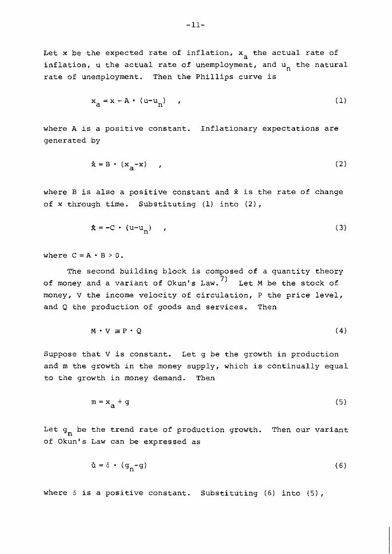
Le t x be t h e expec ted r a t e of i n f l a t i o n , x t h e a c t u a l r a t e of a i n f l a t i o n , u t h e a c t u a l r a t e of unemployment, and u t h e n a t u r a l n r a t e of unemployment. Then t h e P h i l l i p s cu rve i s

where A i s a p o s i t i v e c o n s t a n t . I n f l a t i o n a r y e x p e c t a t i o n s a r e

genera ted by

where B i s a l s o a p o s i t i v e c o n s t a n t and K i s t h e r a t e o f change

o f x th rough t i m e . S u b s t i t u t i n g (1) i n t o (2 ) ,

where C = A m B > O .

The second b u i l d i n g b lock is composed of a q u a n t i t y t heo ry

o f money and a v a r i a n t o f Okun's Law. ') L e t M be t h e s t o c k of

money, V t h e income v e l o c i t y o f c i r c u l a t i o n , P t h e p r i c e l e v e l ,

and Q t h e p roduc t ion o f goods and s e r v i c e s . Then

Suppose t h a t V i s c o n s t a n t . Le t g be t h e growth i n p roduc t ion

and m t h e growth i n t h e money supp ly , which i s c o n t i n u a l l y equa l

t o t h e growth i n money demand. Then

Le t gn be t h e t r e n d r a t e of p roduc t ion growth. Then o u r v a r i a n t

o f Okun's Law can be exp ressed a s

where 6 i s a p o s i t i v e c o n s t a n t . S u b s t i t u t i n g (6 ) i n t o ( 5 ) ,

S u b s t i t u t i n g (1) i n t o (7),

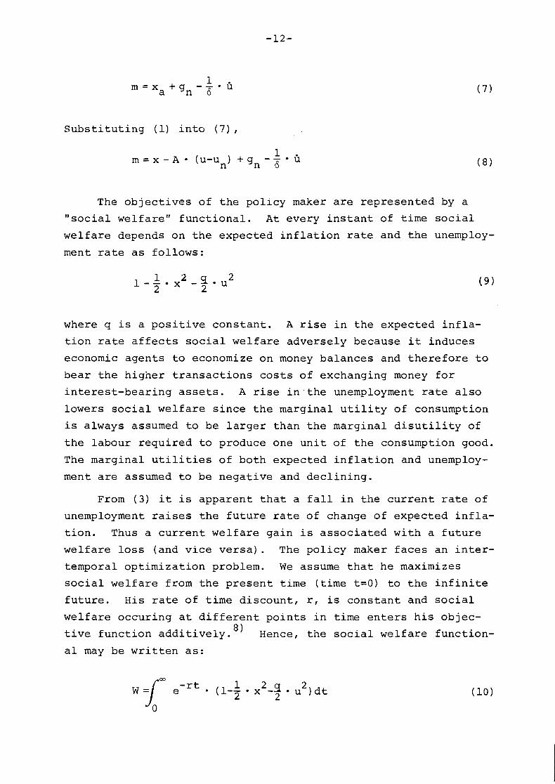
The o b j e c t i v e s o f t h e p o l i c y maker a r e r e p r e s e n t e d by a

" s o c i a l we l f a re " f u n c t i o n a l . A t every i n s t a n t of t i m e s o c i a l

w e l f a r e depends on t h e expec ted i n f l a t i o n r a t e and t h e unemploy-

ment r a t e a s fo l lows :

where q i s a p o s i t i v e c o n s t a n t . A r ise i n t h e expec ted i n f l a -

t i o n r a t e a f f e c t s s o c i a l w e l f a r e adve rse l y because it i nduces

economic agen ts t o economize on money ba lances and t h e r e f o r e t o

b e a r t h e h ighe r t r a n s a c t i o n s c o s t s o f exchanging money f o r

i n t e r e s t - b e a r i n g a s s e t s . A r ise i n t h e unemployment r a t e a l s o

lowers s o c i a l w e l f a r e s i n c e t h e marg ina l u t i l i t y o f consumption

i s always assumed t o be l a r g e r t han t h e marg ina l d i s u t i l i t y of

t h e l abou r r e q u i r e d t o produce one u n i t of t h e consumption good.

The marg ina l u t i l i t i e s o f bo th expected i n f l a t i o n and unemploy-

ment a r e assumed t o be n e g a t i v e and d e c l i n i n g .

From ( 3 ) it i s appa ren t t h a t a f a l l i n t h e c u r r e n t r a t e o f

unemployment r a i s e s t h e f u t u r e r a t e o f change o f expec ted i n f l a -

t i o n . Thus a c u r r e n t w e l f a r e g a i n i s a s s o c i a t e d w i t h a f u t u r e

we l f a re l o s s (and v i c e v e r s a ) . The p o l i c y maker f a c e s an i n t e r -

temporal o p t i m i z a t i o n problem. W e assume t h a t he maximizes

s o c i a l we l f a re from t h e p r e s e n t t i m e ( t i m e t = O ) t o t h e i n f i n i t e

f u t u r e . H i s r a t e of t i m e d i scoun t , r, i s c o n s t a n t and s o c i a l

we l f a re occur ing a t d i f f e r e n t p o i n t s i n t i m e e n t e r s h i s ob jec -

t i v e f u n c t i o n a d d i t i v e l y . 8, Hence, t h e s o c i a l we l f a re f unc t i on -

a l may be w r i t t e n a s :

I n sum, t h e po l i cy problem i s t o maximize ( 1 0 ) s u b j e c t t o (3)

and ( 8 ) , where m i s t h e c o n t r o l v a r i a b l e and x and u a r e t h e

s t a t e v a r i a b l e s . Note t h e m i s no t an argument of t h e s o c i a l

we l fa re f u n c t i o n a l ; t h e r e a r e no po l i cy ins t rument adjustment

cos ts . Assume f o r t h e moment, t h a t m can be changed i n s t a n t a -

neously by i n f i n i t e l y l a r g e amounts; thereby g iv ing r i s e t o in -

s tan taneous , f i n i t e changes of u, a s determined v i a Equation ( 8 ) .

Then, t h e po l i cy problem may be r e s t a t e d i n the fo l lowing, s i m -

p l e r form:

00

1 = / e - . ( l-T . x2-9 - u2) d t . 2 Jo

s u b j e c t t o 3r = -C (u-un) ,

where x i s t h e only s t a t e v a r i a b l e and u may be termed a "sur ro -

g a t e c o n t r o l v a r i a b l e " . However, it i s w e l l known ( s e e , f o r

example, Markus and Lee 1967) t h a t t h e opt imal c o n t r o l u f o r t h e

problem (11) i s a d i f f e r e n t i a b l e func t ion of t ime. Thus, t h e

opt imal G i s w e l l de f i ned and given t h i s G along w i th t h e o p t i -

mal t r a j e c t o r i e s f o r u and x, we can compute t h e opt imal m from

( 8 ) . Consequently, m i s cont inuous w i th r e s p e c t t o t ime and s o

t h e d iscont inuous changes i n m , assumed above, a r e n o t r e a l l y

needed. Hence, t h e t r a j e c t o r y of m which keeps u on t h e pa th

p resc r ibed by op t im iza t i on problem (11) i s opt imal w i th regard

t o t h e maximization of ( 1 0 ) s u b j e c t t o (3) and (8 ) . Thus, u may

be used a s a c o n t r o l v a r i a b l e i n problem (11) even though it

e n t e r s a s a s t a t e v a r i a b l e i n t h e o t h e r problem.

Problem (11) s e r v e s a s our b a s i c model. The extended model

may d i f f e r from t h e b a s i c one i n var ious ways. I n t h e case of

mistaken parameter e s t i m a t e s , t h e d i f f e r e n t i a l equat ion of t h e

extended model may be w r i t t e n a s

where (S-C) o r (8,-u ) i s a measure of t h e mistake i n parameter n es t imat ion . For t h e sake of b r e v i t y , we w i l l cons ider only t h e

case of a mistake es t ima te of un.

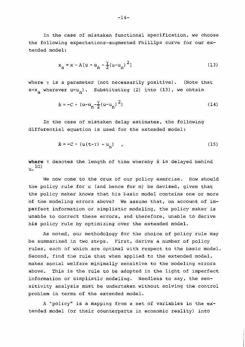
I n t h e case of mistaken func t i ona l s p e c i f i c a t i o n , we choose

t h e fo l lowing expectations-augmented P h i l l i p s curve f o r our ex-

tended model:

2 x = x - A [ u - u u - u I a n 2 (13)

where y i s a parameter ( n o t n e c e s s a r i l y p o s i t i v e ) . (Note t h a t

x=x wherever u=u ) . S u b s t i t u t i n g ( 2 ) i n t o ( 1 3 ) , we o b t a i n a n

I n t h e case of mistaken de lay es t ima tes , t h e fo l lowing

d i f f e r e n t i a l equat ion i s used f o r t h e extended model:

where T denotes t h e l eng th of t ime whereby k i s delayed behind

u. 10

I.Je now come t o t h e crux of our po l i cy exe rc i se . How should

t h e po l i cy r u l e f o r u (and hence f o r m) be dev ised, g iven t h a t

t h e po l i cy maker knows t h a t h i s h a s i c model con ta ins one o r more

of t h e modeling e r r o r s above? We assuns t h a t , on account of i m -

p e r f e c t in format ion o r s i m p l i s t i c modeling, t h e po l i cy maker i s

unable t o c o r r e c t t h e s e e r r o r s , and t h e r e f o r e , unable t:o d e r i v e

h i s po l i cy r u l e by opt imiz ing over t h e extended model.

A s noted, our n~ethodology f o r t h e choice of po l i cy r u l e may

be summarized i n two s t e p s . F i r s t , d e r i v e a number of po l i cy

r u l e s , each of which a r e opt imal wi th r e s p e c t t o t h e b a s i c model.

Second, f i n d t h e r u l e t h a t when app l ied t c t h e extended model,

makes s o c i a l we l fa re minimally s e n s i t i v e t o the modeling e r r o r s

above. Th is i s t h e r u l e t o be adopted i n t h e l i g h t of imper fec t

in format ion o r s i m p l i s t i c modeling. Needless t o say , t h e sen-

s i t i v i t y a n a l y s i s must be undertaken wi thout so l v ing t h e c o n t r o l

problem i n terms of t h e extended model.

A "po l i cy " i s a mapping from a s e t of v a r i a b l e s i n t h e ex-

tended model ( o r t h e i r coun te rpa r t s i n economic r e a l i t y ) i n t o

t h e set o f c o n t r o l v a r i a b l e s . Every p o l i c y which maximizes t h e

s o c i a l we l f a re f u n c t i o n a l w i t h r e s p e c t t o t h e b a s i c model w e

s h a l l c a l l a "bas ic -op t ima l " po l i c y . A number o f d i f f e r e n t po l -

i c ies , a s w e s h a l l see, may a l l be bas ic -op t ima l ; y e t , they may

n o t have t h e same w e l f a r e i m p l i c a t i o n s when a p p l i e d t o t h e ex-

tended model.

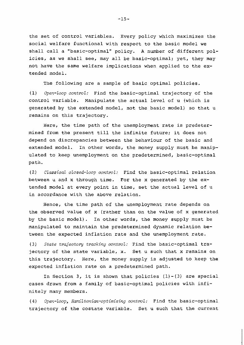
The fo l low ing a r e a sample o f b a s i c op t ima l p o l i c i e s .

(1) Open-loop control: Find t h e bas ic -op t ima l t r a j e c t o r y of t h e

c o n t r o l v a r i a b l e . Manipulate t h e a c t u a l l e v e l o f u (which i s

genera ted by t h e ex tended model, n o t t h e b a s i c model) s o t h a t u

remains on t h i s t r a j e c t o r y .

Here, t h e t i m e p a t h o f t h e unemployment r a t e i s p rede te r -

mined from t h e p r e s e n t till t h e i n f i n i t e f u t u r e ; it does n o t

depend on d i s c r e p a n c i e s between t h e behav iour o f t h e b a s i c and

extended model. I n o t h e r words, t h e money supp ly must be manip-

u l a t e d t o keep unemployment on t h e predetermined, bas ic -op t ima l

pa th .

( 2 ) ClassicaZ closed-loop control: Find t h e bas ic -op t ima l r e l a t i o n

between u and x th rough t i m e . For t h e x genera ted by t h e ex-

tended model a t every p o i n t i n t i m e , set t h e a c t u a l l e v e l o f u

i n accordance w i t h t h e above r e l a t i o n .

Hence, t h e t i m e p a t h o f t h e unemployment r a t e depends on

t h e observed v a l u e of x ( r a t h e r t han on t h e va lue o f x genera ted

by t h e b a s i c model ) . I n o t h e r words, t h e money supp ly must be

manipulated t o ma in ta in t h e predetermined dynamic r e l a t i o n be-

tween t h e expec ted i n f l a t i o n r a t e and t h e unemployment r a t e .

( 3 ) State trajectory tracking control: Find t h e bas ic -op t ima l t r a -

j e c t o r y o f t h e s t a t e v a r i a b l e , x. S e t u such t h a t x remains on

t h i s t r a j e c t o r y . Here, t h e money supp ly i s a d j u s t e d t o keep t h e

expec ted i n f l a t i o n r a t e on a predetermined pa th .

I n S e c t i o n 3 , it i s shown t h a t p o l i c i e s ( 1 ) - ( 3 ) a r e s p e c i a l

c a s e s drawn from a fami l y o f bas ic -op t ima l p o l i c i e s w i t h i n f i -

n i t e l y many members.

( 4 ) Open-loop, Hmiltonian-optimizing control: Find t h e bas ic -op t ima l

t r a j e c t o r y of t h e c o s t a t e v a r i a b l e . S e t u such t h a t t h e c u r r e n t

va lue Hamil tonian, de f ined i n t e r m s of t h e above c o s t a t e v a r i -

a b l e and t h e P h i l l i p s curve of t h e extended model, i s maximized.

H e r e , t h e po l i cy i s t o maximize, a t each p o i n t of t i m e , t h e

observed d i f f e r e n c e between t h e c u r r e n t we l fa re and t h e s o c i a l

c o s t of accumulat ion of i n f l a t i o n a r y expec ta t i ons ( i . e . , t h e

c o s t a t e v a r i a b l e ) . ( 5 ) Closed-loop, Hamiltonian-optimizing control: Find t h e bas ic -

opt imal r e l a t i o n between t h e c o s t a t e v a r i a b l e and t h e expected

i n f l a t i o n x through t ime. For t h e x generated by t h e extended

model a t every p o i n t i n t ime, s e t t h e c o s t a t e v a r i a b l e i n ac-

cordance w i th t h e above r e l a t i o n . S e t u such t h a t t h e c u r r e n t

va lue Hamil tonian, de f i ned i n terms of t h e above c o s t a t e v a r i -

a b l e and t h e P h i l l i p s curve of t h e extended model, i s maximized.

( 6 ) Open-loop, benefit-cost control: Find t h e bas ic-opt imal t r a -

jec to ry of t h e c o s t a t e v a r i a b l e . Define t h e b e n e f i t - c o s t r a t i o

a t a p a r t i c u l a r p o i n t i n t ime t o be s o c i a l we l fa re ( a t t h a t

p o i n t i n t i m e ) d iv ided by t h e s o c i a l c o s t of accumulat ion of in -

f l a t i o n a r y expec ta t i ons ( a t t h a t p o i n t i n t i m e ) , a s g iven by t h e

above c o s t a t e v a r i a b l e and t h e P h i l l i p s curve of t h e extended

model. S e t u such t h a t t h i s bene f i t - cos t r a t i o is maximized a t

every p o i n t i n t i m e .

( 7 ) Closed-loop, benefit-cost control: Find t h e bas ic-opt imal r e l a -

t i o n between t h e c o s t a t e v a r i a b l e and x through t ime. For t h e

x generated by t h e extended model a t every p o i n t i n t ime, set

t h e c o s t a t e v a r i a b l e i n accordance w i th t h e above r e l a t i o n . S e t

u such t h a t t h e bene f i t - cos t r a t i o , de f ined i n t e r m s of t h e

above c o s t a t e v a r i a b l e and t h e P h i l l i p s curve of t h e extended

model, i s maximized a t every p o i n t i n t ime.

A s f o r p o l i c i e s (1) - (3 ) , p o l i c i e s ( 4 ) - ( 7 ) can be combined

t o genera te y e t f u r t n e r po l i cy op t ions . A l l above p o l i c i e s a r e

equ iva len t and opt imal i f t h e extended model i s i d e n t i c a l t o t h e

b a s i c one.

What now remains t o be done is t o spec i f y t hese p o l i c i e s

r i go rous l y and t o f i n d those p o l i c i e s which a r e l e a s t s e n s i t i v e

t o t h e va r ious modeling e r r o r s cons idered above. Th is i s t h e

s u b j e c t of t h e fo l lowing t h r e e s e c t i o n s .

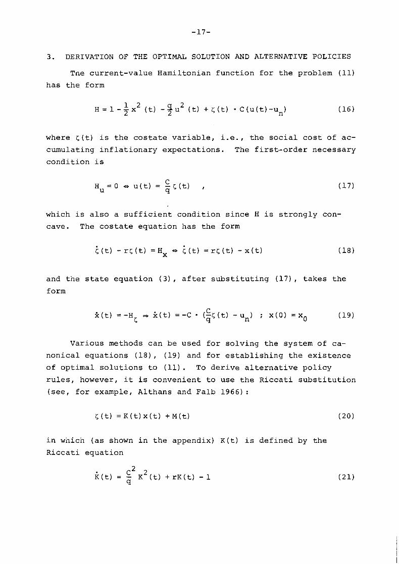
3 . DERIVATION OF THE OPTIMAL SOLUTION AND ALTERNATIVE POLICIES

The cu r ren t - va lue Hami l tonian f u n c t i o n f o r t h e problem (11)

has t h e form

where z;(t) i s t h e c o s t a t e v a r i a b l e , i . e . , t h e s o c i a l c o s t o f ac-

cumula t ing i n f l a t i o n a r y e x p e c t a t i o n s . The f i r s t - o r d e r necessa ry

c o n d i t i o n i s

which i s a l s o a s u f f i c i e n t c o n d i t i o n s i n c e H i s s t r o n g l y con-

cave. The c o s t a t e e q u a t i o n has t h e form

and t h e s t a t e e q u a t i o n ( 3 ) , a f t e r s u b s t i t u t i n g (17) , t a k e s t h e

form

Var ious methods can be used f o r s o l v i n g t h e sys tem o f ca-

n o n i c a l e q u a t i o n s ( 1 8 ) , (19) and f o r e s t a b l i s h i n g t h e e x i s t e n c e

o f op t ima l s o l u t i o n s t o (11). To d e r i v e a l t e r n a t i v e p o l i c y

r u l e s , however, it i s conven ien t t o use t h e R i c c a t i s u b s t i t u t i o n

(see, f o r example, A l thans and F a l b 1966) :

i n whicn ( a s shown i n t h e appendix) K ( t ) i s d e f i n e d by t h e

R i c c a t i e q u a t i o n

and ~ ( t ) by t h e a u x i l i a r y equa t i on

c2 ~ ( t ) = (: ~ ( t ) + r ) ~ ( t ) -CunK( t )

One of t h e s u f f i c i e n t c o n d i t i o n s f o r t h e e x i s t e n c e of o p t i -

mal s o l u t i o n s , i f t h e Hami l tonian f u n c t i o n i s s t r o n g l y concave,

i s t h a t t h e R i c c a t i e q u a t i o n ( 2 1 ) , when so l ved backward i n t i m e ,

has a bounded s o l u t i o n . For t h e equa t i on ( 2 1 ) , such a s o l u t i o n

does e x i s t (see t h e appendix) and has t h e fo l low ing form:

The cor respond ing s o l u t i o n o f (22) i s

Now, s u b s t i t u t i n g ( 2 0 ) , ( 2 3 ) , (24) i n t o ( 9 ) , (10) and so lv -

i n g t h e d i f f e r e n t i a l e q u a t i o n s w e o b t a i n t h e op t ima l s o l u t i o n s

f o r t h e problem (11)

rqun A - rqun

2 (t) = (xo-8_) e -"t+- C ; l i m 2 ( t ) = x W - - C > 0 t+'0

- u t q"n A qUn t ( t ) =K(xo -2_ )e +- C , l i m < ( t) = <, = > 0 t-

A

where 2_, c W , Qw denote op t ima l long-run s o l u t i o n s and

i s a c o e f f i c i e n t measur ing t h e speed w i t h which i n f l a t i o n and

unemployment approach t h e i r r e s p e c t i v e long-run op t ima l v a l u e s .

This speed attains its maximal value when r+O:

L

'max = lim u =T r+O 92

The ratio of this maximal speed to the depreciation rate r

u max - C v=--- r 1

'92

or, more precisely, its squared value v2, plays an important role

as a basic aggregated parameter in the analysis that follows.

Observe, for example, that the ratio u/r, as specified by (28), 1 -

2 1 2 2 is a function of v alone, ~ / r = ~ ( ( l + 4 v ) -1). Suppose the

depreciation rate r is given and fixed, and the parameter v2 is

changed by choosing an appropriate weighting coefficient q; if 2 2 qjm, then v '0, if q+O, then v jm. The graph of u/r as a func-

tion of v2 is given in Figure 1.

Too slow I Reasonable I Too high control I results I sensitivity

I I I

Figure 1. Dependence of the relative speed of control u/r, on C the aggregated parameter v 2 = T.

r q

Since a reasonable va lue of t h e dep rec ia t i on r a t e i s r = 0 . 1 /

year , parameter va lues t h a t r e s u l t i n a r a t i o u / r c 1 might be

cons idered a s n o t acceptab le s o c i a l l y : t h e speed of approaching

long-term s o l u t i o n s i s too slow i n such a case. The r a t i o u / r = l 2 2

i s obta ined by v = 2 , U / r = 4 by v =20. We s h a l l show t h a t a l l

p o l i c i e s become very s e n s i t i v e t o modeling e r r o r s ( i . e . , become

r a t h e r imprac t i cab le ) f o r v 2 much l a r g e r than 20, whi le they re - C1

main robus t f o r v L between 2 and 20. For t h i s range of param- 1 e t e r s ( v 2 - > 2 ) we can a l s o reasonably approximate U by U =C/qy max

and U / r by v ( s e e t h e appendix) .

The opt imal va lue of t h e we l fa re f u n c t i o n a l (10) can be

determined a s a q u a d r a t i c func t ion of xo-9,

where

The term s tands f o r s o c i a l we l fa re i n equ i l i b r i um 0

( cha rac te r i zed , a s noted above, by t h e absence of expec ta t i ona l

e r r o r s ) AG i s t h e f i r s t - o r d e r approximation of we l fa re l o s s e s

due t o an i n i t i a l d i sequ i l i b r i um (cha rac te r i zed by t h e d i f f e r -

ence between t h e i n i t i a l and long-run opt imal r a t e of expected 2 i n f l a t i o n ) , and A W i s t h e second-order approximation of such

l o s s e s . S i m p l i s t i c modeling o r imper fect in format ion i n c r e a s e

such l o s s e s f u r t h e r ; however, t h e a d d i t i o n a l l o s s e s a r e always

of second-order form and s h a l l be thus compared wi th t h e 2A t e r m A W.

Moreover, t h e maximal va lue of t h e Hamiltonian func t i on ,

i n t e r p r e t e d a s a shadow p r i c e f o r pass ing t i m e i s

Before proceeding to the definition of alternative policy

rules, consider the following short-hand description of our

basic and extended models. Define the vectors of parameters

which distinguish the extended from the basic model as

and let Gn=un+f3. The extended model is

-rt(l-;x2 (t) -?U2 (t))dt w=[ e

2 subject to P(t) = -C(u(t-T) - u - B - $(u(t-.r) - u - B) 1 . . n n

We denote this model by M(a). - Clearly, the extended model is identical to the basic model (11) if a=a. We denote the basic - - model by M(a). - The variables of the basic model depend on the

parameter a and will be denoted B(t,a),Q(t,a), etc. We approach - - - the solution to the extended model as that of the basic model

through techniques related to the implicit function theorem.

Now consider alternative policies, all of which are optimal

when applied to the basic model, but which might yield different

solutions when applied to the extended one. The simplest policy

is the open-loop optimal control:

obtained from the basic model and applied to the extended one.

Another policy is the classical closed-loop optimal control

defined by a function Q(t,a) - which depends solely on the current

S(t,a) - and not on the initial value x,. When comparing (25) , CK (27) it is easy to see that Q(t,a)= -jt(t,a) + (1-rK) u when - q - n'

implementing t h i s p o l i c y r u l e i n t h e ex tended model, however,

E t ( t ,a ) - i s s u b s t i t u t e d by expected i n f l a t i o n x ( t ) t a k e n from t h e

ex tended model. Thus, t h e c l a s s i c a l c losed- loop op t ima l c o n t r o l

i s

uC ( x ( t ) ,a) = s x (t) + ( 1 - r K ) un 9

(39)

Another a l t e r n a t i v e p o l i c y i s t h e op t ima l t r a j e c t o r y t r a c k -

i n g c o n t r o l :

t u ( x ( t ) ,a) = { U (t) such t h a t x ( t ) = S ( t , a ) - 1 (40)

whicn means t h a t t h e r a t e of expec ted i n f l a t i o n x ( t ) which

emerges from t h e ex tended model i s main ta ined a t t h e p re -

determined p a t h S ( t , a ) . -

A l l t h e s e a l t e r n a t i v e p o l i c y r u l e s (38) , ( 3 9 ) , (40) a r e

members o f an i n f i n i t e fami l y of c losed- loop c o n t r o l s parameter-

i z e d by a c o e f f i c i e n t A :

X 0 X I f A = O , t hen u ( x ( t ) ,a) = u ( t , ~ ) . I f X = l , t nen u ( x ( t ) ,a) =

uC ( x ( t) ,a) . If t h e ex tended model (37) t aken t o g e t h e r w i t h t h e

p o l i c y r u l e (41) remain s t a b l e a s A+.. which can be shown t o be X t h e c a s e i f T = O , t h e n it i s easy t o check t h a t u ( x ( t ) , a ) - +

t u ( x ( t ) ,a) .

For i n t e r m e d i a t e v a l u e s of A , however, w e have a pa rame t r i c

p o l i c y r u l e which d i c t a t e s t h a t a l i n e a r combinat ion o f unemploy-

ment and expec ted i n f l a t i o n , observed from t h e ex tended model,

C * K x (t) f o l l o w t h e predetermined p a t h 8 (t . a ) ~ ( t ) - A - '1 -

CK - A - - B ( t , a ) . 9 - Aside from t h i s i n f i n i t e number of p o l i c y r u l e s , t h e s e a r e

y e t f u r t h e r p o s s i b i l i t i e s . S ince t h e op t ima l c o n t r o l maximizes

t h e Hami l tonian f u n c t i o n ( 1 6 ) , t h e p o l i c y maker may employ i n

t h e open-loop Hami l tonian maximizing feedback (see Wierzb ick i

1977) :

1 2 2 A =argmax (1--x i t ) - $ u ( t) - ~ ( t , a ) * f ( u ( t ) , a ) ) 2

w i tn u ( t ) , x ( t ) a r e taken from t h e extended model, and f ( u ( t ) ,g) = k ( t ) i s t h e d e r i v a t i v e of s t a t e v a r i a b l e a s measured i n t h e

extended model. I n o t h e r words, w e compute t h e va lue of t h e

c u r r e n t we l fa re func t i on and, us ing t h e P h i l l i p s curve of t h e

extended model a s we l l a s t h e shadow p r i c e f o r t h e accumulat ion

of i n f l a t i o n a r y expec ta t i ons t ( t , a ) - , we maximize t h e d i f f e r e n c e

between t h e c u r r e n t we l fa re and t h e c o s t of f u t u r e i n f l a t i o n .

However, w e need n o t use a predetermined shadow p r i c e ' t (t , - a ) ;

s i n c e we a l s o know i t s c lose- loop form t ( t , a ) - = & ( t , a ) - + M I we

could a l s o use t h e measured x ( t ) f o r c o r r e c t i o n s of t h i s shadow

p r i c e . Th is r e s u l t s i n t h e closed-loop Hamiltonian maximizing

feedback:

1 2 2 = argmax ( l - T ~ (t) - $ u (t) - LKx ( t ) + H) f (u (t) I : ) ) u( t)

The Hamiltonian func t i on ( 1 6 ) can a l s o be r e w r i t t e n i n a d i f f e r -

e n t form. For example, t h e r e l a t i o n

1 2 2 l - Z ~ (t) - 3 u ( t )

u f o ( t (t Ia) , t t ( t I g ) ,a) = argmax u ( t ) ? ( t , ~ ) = f ( u ( t ) Ia)+t t ( t Ia)

y i e l d s a l s o u f O ( t ( t I a ) , tT ( t ,a ) ,a) = G ( t , a ) - a t - a=a; - whi le i t might

y i e l d d i f f e r e n t s o l u t i o n when - a f a . - Th is i s t h e open-loop,

bene f i t - cos t c o n t r o l . Observe t h a t i f t ( t ,a )=O would ho ld , t - then t ( t , a ) - would n o t a f f e c t t h e maximization i n ( 4 4 ) and t h e

r e s u l t i n g ufo ( t ( t , - a ) ,0 ,a) =G (t,a) - would be opt imal f o r t h e ex-

tended model no mat te r what e r r o r s a f a were made i n t h e b a s i c - - model. Thus, t h e b e n e f i t - c o s t c o n t r o l i s p e r f e c t l y robus t i f

t h e c o s t of pass ing t ime i s n e g l i g i b l e . However, i n t h e example

A

considered here, ct(tIa) - # O and it will be shown that this con-

trol policy has some undesirable properties.

If tt(t,a) #0, then the errors in determining the shadow

prices can be corrected in a close-loop structure

1 2 (t)-qu 2 (t,

= argmax (45) u(t) (Kx(t)+Ml f (u(t) ,a)+tt(x(t) - tg )

where (x(t) ,a) is determined as in (35) but with u!t) and (t) t -

substituted by (17) , (20) ; x (t) is taken from the extended model.

Clearly, it would be possible to generate yet other policy

rules, each involving observations from variables from the ex-

tended model and a scheme for influencing these variables which

is basic-optimal (i.e., yield optimal solutions whenever - a=a). - However, we restrict our attention to the policy rules listed

above. If the probability distributions of the model parameters

were known, then a dual stochastic optimal control and estima-

tion problem could be formulated and possibly solved. Yet,

such problems are notoriously difficult. In this paper we

concentrate on the derivation of policy rules when the param-

eter distributions are not known. Such conditions call for a

different methodology, to which the following section is devoted.

4. METHODOLOGY OF ROBUSTNESS ANALYSIS

i Consider a given policy rule u , mapping the variables

measured in the extended model into the control actions for this

model. This policy is defined with the help of the basic model

and thus depends on parameters - a (see Figure 2).

Suppose it is at least conceptually possible to solve the i extended model under this policy rule, thus obtaining x (t,a,a) - -

i and u (t,a,a); - - these results depend on the policy rule i as well

as on the parameters - a,a. - Similarly, suppose we could compute

the social welfare functional of the extended model under this

policy rule:

If we were able to optimize the extended model and compute

the corresponding social welfare functional fi (a) - , we would find

that wi (a, a) < fi (a) , since the differences between the basic - - - - model and the extended one (a - # - a) imply that the policy rule

may not be optimal for the extended model. Thus, as a measure

of the robustness of a policy rule, we use the welfare loss of

applying this rule to the extended model:

However, since the extended model is more complicated than A

the basic one, a direct computation of W(a) - and si (a,a) - - may be

impossible. On the other hand, the function si (a,a) - - has several

useful properties that facilitate its approximation even i f only

the solutions of the basic model, but not those of the extended model are i hm. First, S (a, - - a) is non-negative:

i si (oi,a) L 0 ; S ( 2 , ~ ) = 0 for all - a = - a

Therefore, if si is differentiable, its first-order derivatives

are zero for all a=a: - -

It follows further (see Wierzbicki 1977) that if si is twice

differentiable, its second-order derivatives have a specific

symmetry property:

i There fo re , S ( a , a ) - - can be approximated by

where o ( - ) i s a f u n c t i o n converging t o zero f a s t e r t han i t s ~i

argument. A s a n e x t s t e p , w e need a method f o r computing S a a . i - -

I f w e could approximate t h e d i f f e r e n c e s between x ( t , a , a ) , - - u i ( t f a f a ) and P ( t , a ) - , C ( t , a ) - which would be op t ima l f o r t h e ex-

tended model

then w e could e a s i l y 12) determine t h e q u a d r a t i c form of t h e

approximat ion (51) :

13) However, xi (t) and ;i (t) , c a l l e d extended structural variations , a r e u s u a l l y n o t d i r e c t l y computable. I t i s u s u a l l y s imp le r t o

compute t h e basic structural variations

i x (tf2,a) - f ( t , a ) = - x i ( t ) (2-5) + o ( 1 ~ a - ~ l - 1 )

(54)

ui (trnra) - Q(t ,a) = ii (t) (a-a) - - + o ( 1 ( E - a l I ) .

These approximate t h e d i f f e r e n c e between t h e extended model (un-

derg iven p o l i c y r u l e , o r i n g iven control structure) and t h e o p t i -

mal s o l u t i o n s i n t h e b a s i c mode. W e wish t o exp ress t h e ex-

tended s t r u c t u r a l v a r i a t i o n s , i n ( 5 3 ) , v i a t h e b a s i c s t r u c t u r a l

v a r i a t i o n s minus t h e b a s i c op t ima l v a r i a t i o n s :

For t h i s purpose, w e must compute t h e b a s i c op t ima l v a r i a t i o n s :

Q ( t 1 a ) - - Q ( t , a ) - = u ( t ) - (a-a) - - + o ( l la-a1 - - 1 )

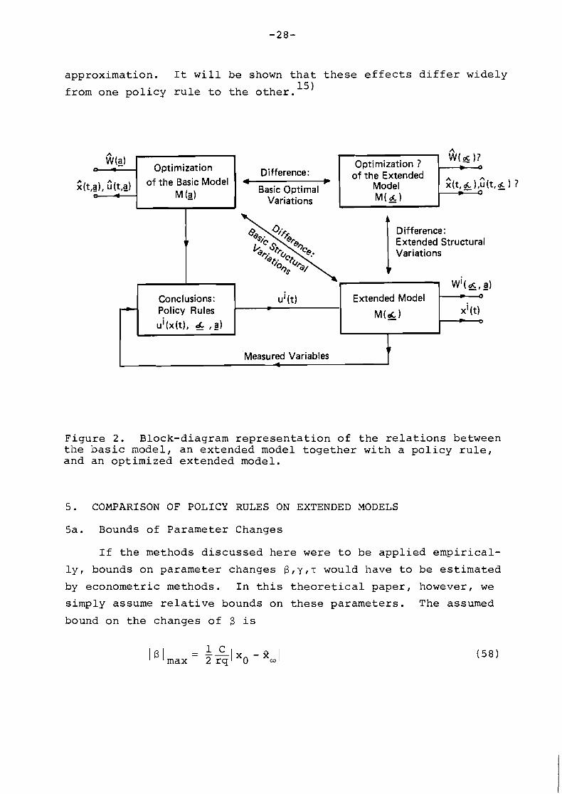
The i n t e r r e l a t i o n s among t h e o p t i m i z a t i o n s o f t h e b a s i c

model, t h e ex tended model, and t h e s o l u t i o n o f t h e b a s i c model

under g i ven p o l i c y a r e i l l u s t r a t e d i n F igu re 2 . The u s e f u l n e s s

o f t h e method above l i es i n t h e f a c t t h a t although the extended model

might be d i f f i c u l t t o optimize or t o solve exp l i c i t l y mder given policy rule,

the variational equations that determine the basic optimal variations and

basic structural variations are usually much simpler thun the extended model

i t s e l f . The reason i s t h a t t h e s e v a r i a t i o n a l e q u a t i o n s a r e so l ved

a long t h e s o l u t i o n s o f t h e b a s i c model, a t t h e parameter v a l u e - a .

For example, i f t h e ex tended model c o n t a i n s de layed v a r i a b l e s ,

t h e v a r i a t i o n a l e q u a t i o n s r e l a t e d t o t h e i n f l u e n c e o f t h e d e l a y

a r e n o t de layed themselves.

Observe now t h a t i f a i s a column v e c t o r o f p pa ramete rs , - iri (t) and iii (t) a r e , i n f a c t , row v e c t o r s o f p v a r i a t i o n s co r re -

i T sponding t o t h e s e parameter changes; t h u s x (t) xi ( t ) and i uiT ( t ) u (t) a r e pxp m a t r i c e s . The ma t r i x .?: a t h u s has t h e

14 - - form

I n o r d e r t o a n a l y s e f u l l y t h e approx imat ion ( 5 1 ) , w e shou ld

a c t u a l l y compute t h e m a t r i x 6; a , e s t i m a t e independen t l y some - -

bounds on t h e changes - a-a, - and approximate upper bounds f o r (51)

by e i genva lue a n a l y s i s . Though such an a n a l y s i s i s s t r a i g h t f o r -

ward, y e t , f o r t h e sake of s i m p l i c i t y , w e s h a l l on l y compute t h e

d i agona l e lements o f 8: a , use some upper bounds on t h e e lements - -

o f - a-a, - and compare t h e r e s u l t s f o r each e lement of t h i s v e c t o r

independent ly . The reason f o r t h i s s i m p l i f i c a t i o n i s t h a t w e do

n o t wish t o c o n c e n t r a t e on j o i n t e f f e c t s o f t h e changes o f v a r i -

ous components of - a . Ra ther , w e would l i k e t o i n v e s t i g a t e t h e

s e p a r a t e e f f e c t s o f each p o l i c y r u l e on t h e w e l f a r e l o s s

approximation. It will be shown that these effects differ widely

from one policy rule to the other. 15

I Measured Variables t

A

Figure 2. Block-diagram representation of the relations between the basic model, an extended model together with a policy rule, and an optimized extended model.

W (5) o e

G ( t # i ) # fi(t#il)

5. COMPARISON OF POLICY RULES ON EXTENDED MODELS

5a. Bounds of Parameter Changes

Optimization ? Optimization Difference: of the Extended

of the Basic Model p Basic Opt~mal Model M (a) Variations

If the methods discussed here were to be applied empirical-

ly, bounds on parameter changes f 3 , y , ~ would have to be estimated

by econometric methods. In this theoretical paper, however, we

simply assume relative bounds on these parameters. The assumed

bound on the changes of f3 is

1r Difference: Extended Structural Variations

-C

Conclusions: Extended Model Policy Rules - - ui(x(t), 4 , ? I

i . e . , t h e e r r o r i n e v a l u a t i n g u is r e l a t e d t o t h e d ive rgence n ' between t h e a c t u a l and long-term expec ted r a t e s o f i n f l a t i o n ,

and t h u s a l s o t o t h e d ive rgence between t h e a c t u a l and n a t u r a l C r a t e o f unemployment ( s i n c e @=ii -u and u =On, =-Stm see t h e n n n Sq append ix ) . W e assume a l s o t h a t t h e e r r o r i n yun i s of s i m i l a r

n a t u r e

F i n a l l y , f o r t h e d e l a y T w e assume a r e l a t i v e bound

T - - 1 -d max 4umax - 4C

s i n c e t h e r e l a t i v e e f f e c t s o f an over looked de lay T a r e charac-

t e r i z e d by t h e number U T (see t h e append i x ) .

5b. S e n s i t i v i t y t o E r r o r s i n Es t ima t i ng Na tu ra l Unemployment Rate

I n t h i s s imp le case w e know t h e op t ima l s o l u t i o n s f o r t h e

ex tended model, j u s t s u b s t i t u t i n g u by an i n (25) , ( 2 6 ) , ( 2 7 ) . n Thus, t h e b a s i c op t ima l v a r i a t i o n s a r e ob ta ined immediate ly

w i t h B = i i -u w e assume B f O , y=O, T = O i n t h i s s u b s e c t i o n and n n' deno te k ( t , a ) = S ( t , B ) , - G ( t , a ) = Q ( t , B ) - i n t h i s case . The b a s i c

s t r u c t u r a l v a r i a t i o n s depend on an assumed p o l i c y r u l e . Con- s i d e r f i r s t t h e f am i l y o f c losed- loop c o n t r o l s (41) and s u b s t i -

t u t e it i n t o t h e ex tended s t a t e equa t i on (12) t o o b t a i n (assum-

i n g C=C) :

. X X x ( t ) = -C (U (t) - u n ) = - c ( Q ( t , a ) - f i " - n + ~ - ( x CK (=I x ( t , a ) ) ) - ;

X x ( 0 ) = x 0 (62)

Again, i n t h i s r e l a t i v e l y s imple c a s e w e can s o l v e t h e ex tended

model a n a l y t i c a l l y :

and determine t h e b a s i c s t r u c t u r a l v a r i a t i o n s

i ( x A ( t) - f ( t , a ) ) = iiA(t) = A- (1 - e - A u t ACK 1

1 . A - A - A u t - (u ( t) - Q ( t , a ) ) = u (t) = 1 - e B -

which, i n t u r n , i m p l y t o g e t h e r w i t h (61) , (56) t h e extended

s t r u c t u r a l v a r i a t i o n s

Now w e can compute t h e second-order d e r i v a t i v e o f t h e w e l f a r e A l o s s e s S ( a , a ) - - wi th r e s p e c t t o 8:

A I n t h i s s imple c a s e t h e f u n c t i o n S ( a , a ) - - i s a q u a d r a t i c

f u n c t i o n o f 6 ; hence t h e w e l f a r e l o s s e s a s s o c i a t e d w i t h B a r e

2 A A . I n o r d e r t o o b t a i n a c o e f f i c i e n t of r obus tness which 7B S B ~ does n o t depend on u n i t s o f measurement, w e use t h e r a t i o o f 2

'ma, and a26' ( t h e r a t i o o f l o s s e s due t o i n e x a c t parameter B B

e s t i m a t i o n t o n a t u r a l l o s s e s due t o an i n i t i a l d i s e q u i l i b r i u m

If X=O, for the open-loop policy, this robustness coefficient

takes the form

For A=l, the classical closed-loop policy, we obtain

and for A+a, the optimal trajectory tracking policy:

We can also determine the feedback coefficient that minimizes B (67) and thus provides for the best robustness in this policy

family:

All these results depend on the parameters rK, which are deter- c2 mined, via (23) , by the parameters - = v2, the squared ratio r q

of the maximal speed of controlling inflation and unemployment, - - -

'max to the time discount rate r. Thus, when analysing 1' q'

robustness coefficient graphically, we shall employ the parameter 1 I

2 v2 instead of r ~ = ( (l+lv2)' - 1)/2v .

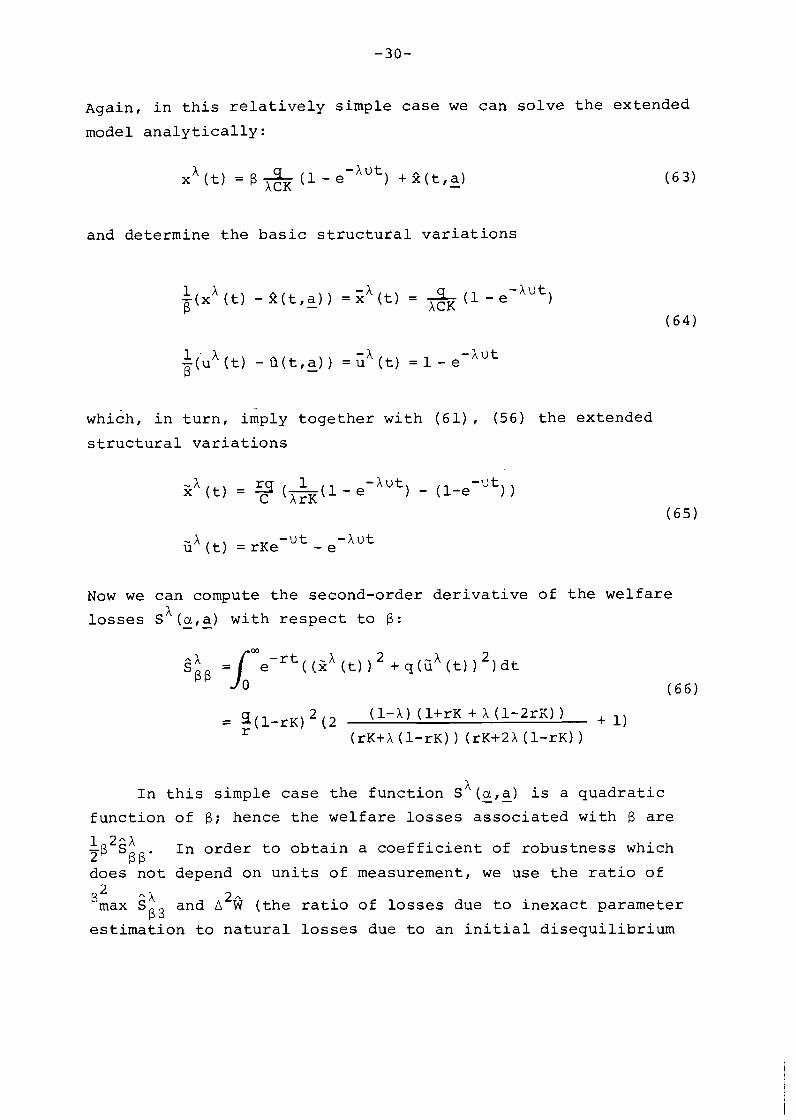
A X F igure 3. Dependence of t h e robustness c o e f f i c i e n t R on v 2

and A . B

The graphs of 2' a s a func t ion of v2 and A , presented i n B Figure 3 i n d i c a t e dramat ic changes of robustness--upto l o 3 t imes

and over--depending on t h e choice of A. Th is can be i n t e r p r e t e d

i n t n e fo l lowing way. When t h e at tempt t o mainta in p r e c i s e l y a

predetermined pa th of unemployment ( a t X = O ) o r a predetermined

path of expected i n f l a t i o n ( a t X-) i s made, even s l i g h t e r r o r s

i n t h e eva lua t i on of t h e n a t u r a l unemployment r a t e un can r e s u l t

i n l a r g e we l fa re l o s s e s . However, i f an app rop r ia te combination CK of unemployment and expected i n f l a t i o n , Q ( t , a ) - X - - 8(t,5) wi th 9

h c l o s e t o i i s chosen a s a po l i cy t a r g e t , smal l e r r o r s i n t h e B '

eva lua t i on of u do n o t cause s i g n i f i c a n t we l fa re l o s s e s . W e , n however, s e e t h a t even t h e choice of X cannot reduce we l fa re

l o s s e s s u f f i c i e n t l y , i f t h e parameter v2 becomes much l a r g e r

than 20--which would correspond t o t h e d e s i r e of ob ta in ing f a s t

r e s u l t s i n c o n t r o l l i n g i n f l a t i o n (h igh v / r , s e e F igure 1) by

a t t a c h i n g a smal l weight q t o unemployment.

Consider now the open-loop Hamiltonian maximizing policy:

1 2 2 = argmax (l-rx it) - 9 u (t) + t(t,a) C (u(t) -Gn)) u(t)

2

The fact that we measure the accurate current speed of change of - inflationary expectations, k (t) = -C ( u (t) - un) , does not inf lu-

ence the maximization in (72); no matter what Gn is taken, we

obtain

Thus, the open-loop Hamiltonian maximizing policy is equivalent

to the simple open-loop policy, if no changes of the functional

form of the Phillips curve are considered. Similarly, it can

be shown for this case that

the closed-loop Hamiltonian maximizing policy is equivalent to

the classical closed-loop policy. Since the simple open-loop

and the classical closed-loop are not the best choices from our

given set of policy options, it is not desirable to pursue

Hamiltonian maximizing policies.

The benefit-to-cost optimizing policies perform even more

poorly. 3y setting f (u (t) ,g) = -C (u (t) -un-8) and computing the

maximum of (43) we obtain16)

f 0 fo A 1 2 where u (t)=u (~(t.2). St(t,a) .a) - and U(%,Q.a)=l- - T f .(t,g)

- 9Q2 (t,a) for the sake of notational economy; xfO (t) denotes 2 - here the state x(t) measured in the extended model under the

po l i cy r u l e (75) . Now, i f we s u b s t i t u t e (75) i n t o t h e extended £0 £0

model R (t) = -C ( u (t) -un-B) , we o b t a i n a non l inear d i f f e r e n -

t i a l equat ion

A s noted i n t h e preceding s e c t i o n , we do n o t have t o so l ve t h i s £0

equat ion. I t i s s u f f i c i e n t t o l i n e a r i z e it i n B a t B=0, x ( t )=

- 17 8 ( t , a ) t o o b t a i n t h e equat ions f o r b a s i c s t r u c t u r a l v a r i a t i o n s .

2 ' £0 Q ( t , a ) S ( t , a ) - - :fo qu (tta) x (t) = C ( t ) + c ( U(8.Q.a) + 1 ;

u (B,Q,a)

- fo qfi2 (tra) Q ( t , a ) f - ( t , a ) - -fo u (t) = - - u(Q,Q,a) u (Q,Q,a) x (t)

When tak ing i n t o account (56) , (61) , we d e r i v e a l s o t h e equat ions

f o r extended s t r u c t u r a l v a r i a t i o n s

The d i f f e r e n t i a l equat ions i n both (77) and (78) a r e uns tab le i f

u(A,Q,a)>O - which occurs when f t ( t , a ) , C i ( t , a ) a r e s u f f i c i e n t l y - - smal l . Thus, a l s o t h e equat ion (76) i s uns tab le18) , i f

U ( k , Q , a ) > 0 . I n o t h e r words, t h e b e n e f i t - t o - c o s t maximizing

p o l i c y i n v a r i a b l y l e a d s t o u n s t a b l e r e s u l t s wherever t h e r e a r e

e r r o r s i n t h e e v a l u a t i o n o f t h e n a t u r a l unemployment r a t e . On

t h e o t h e r hand, t h i s does n o t imply t h a t t h e we l f a re l o s s under

t h i s p o l i c y i s n e c e s s a r i l y i n f i n i t e ; it might be f i n i t e i f r>>

Q ( t , a ) A ( t , a ) - u(A IQIa ! f o r a l l t. However, even i n such a c a s e , when

- f o - £0 computing x ( t ) , u (t) under somewhat s i m p l i f y i n g assumpt ion

t h a t ~ ~ = 2 ~ (see t h e appendix) it can be shown t h a t

which imp l i es t h a t t h e w e l f a r e l o s s under t h e b e n e f i t - t o - c o s t

maximizing p o l i c y i s l a r g e r than under t h e s imple open-loop

p o l i c y . S ince a s i m i 1 a r : r e s u l t can be d e r i v e d f o r t h e c losed-

loop bene f i t - t o - cos t maximizing p o l i c y , w e conclude t h a t t h e s e

p o l i c i e s a r e n o t d e s i r a b l e ways o f d e a l i n g w i t h t h e problems o f

i n f l a t i o n and unemployment w i t h i n o u r a n a l y t i c a l c o n t e x t . 19 )

5c. S e n s i t i v i t y t o Mistaken Func t i ona l S p e c i f i c a t i o n

W e assume h e r e t h a t - a=(O,y ,O) , i . e . , t h e ex tended model

t a k e s t h e form:

The problem of maximizing (10) s u b j e c t t o (80) does n o t admi t an

a n a l y t i c s o l u t i o n ; however, t h i s problem has s o l u t i o n s f o r su f -

f i c i e n t l y sma l l y and t h e s e s o l u t i o n s a r e d i f f e r e n t i a b l e i n y .

Th i s can be seen by w r i t i n g t h e Hami l tonian f u n c t i o n f o r t h i s

problem

and t h e necessary c o n d i t i o n s o f o p t i m a l i t y

and observ ing t h a t t h e Hami l tonian f u n c t i o n remains concave f o r

s u f f i c i e n t l y sma l l y and a cor responding R i c c a t i equa t i on has a

backward s t a b l e s o l u t i o n which depends d i f f e r e n t i a b l y on t h e

parameter y; s i m i l a r l y , t h e s o l u t i o n s o f ( 8 4 ) , (82) depend then

d i f f e r e n t i a b l y on y. However, w e omi t t h e s e d e t a i l s h e r e , and

show on l y how t o d e r i v e b a s i c v a r i a t i o n a l equa t i ons . , .

Denote t h e s o l u t i o n s o f t h i s problem by G ( t , Y ) =Q ( t , a ) + ~ u ( t ) A A

- A

+ o ( y ) ,~(t,~)=S(t,a)+yZ(t)+o(y), - c ( t , y ) = ? ( t , g ) + ~ t ( t ) + o ( ~ ) and

rewrite t h e equa t i ons (82) , (83) , (84) a s

S ince t h e exp ress ions i n square b r a c k e t s a r e zeros--cf . ( 1 7 ) ,

( 1 8) , ( 1 9 ) --we subd iv ide t h e remainders by y and l e t y+O t o

o b t a i n

C A since - r; (t, - a) =Q (t, - a) ; the last equation is obtained by taking

into account (88). Observe that, if Q(t,a)=un, under initial A A

- equilibrium conditions, then t ( t ) ~ 0 , ;(t)-0. If Q(t,g)-un

increases, which might be caused by an increase of xO-kmf then A A

also (t) and ; (t) will, in general, increase. Thus, the sensi-

tivity of optimal solutions to the parameter y increases with

the distance from equilibrium. While it is possible to solve

the equations (89), (90) in their general form, we can signifi-

cantly simplify computations by assuming approximately that

Q(t,a)-u - = u that is, by solving these equations at a stan- n n' dard distance from equilibrium. In this case, we obtain

Consider now the family of closed-loop policies (41). The

extended model equation under these policies takes the form

X KC A (t) =-C(Q(t,g) - u n + X - (X (t) -k(t,g)) 9

Again, the solutions of this equation are differentiable func- X X

tions of y, x (t)=2(t,a)+yxh - (t)+~(~). u (t)=O.(t.a)+y;A (t)+o(y) . When linearizing (92) by the same technique as applied for (82),

(83), (84) , we obtain

Z A 1 K~~ ;A (t) + C (Q(t.a) - un) x (t) = - A - - ; xA(0)=O ci

Under the approximative assumption Q (t, - a) -u % un, (93) yields n

- A 1 u 3 - - A x (t) a (l-e 1 2 hut) ; u (t) a - u (I-e 2 n (94) 1

The basic structural variations xA(t) (t) and the basic opti- A A

ma1 variations z(t) ,u(t) determine extended structural variations

(t) , 1 u2 3 (- I (1-e - 5 ( -e-Ut) ) 2 n C ArK

and, in turn, the second-order derivative of the welfare loss

A dimensionless robustness coefficient is

and it takes the following forms for A=O (open-loop policy),

A=l (classical closed-loop policy) and A- (optimal trajectory

tracking) :

The feedback coefficient ^A that minimizes (97) , thus providing Y

for the most robust policy from this family, can be determined as

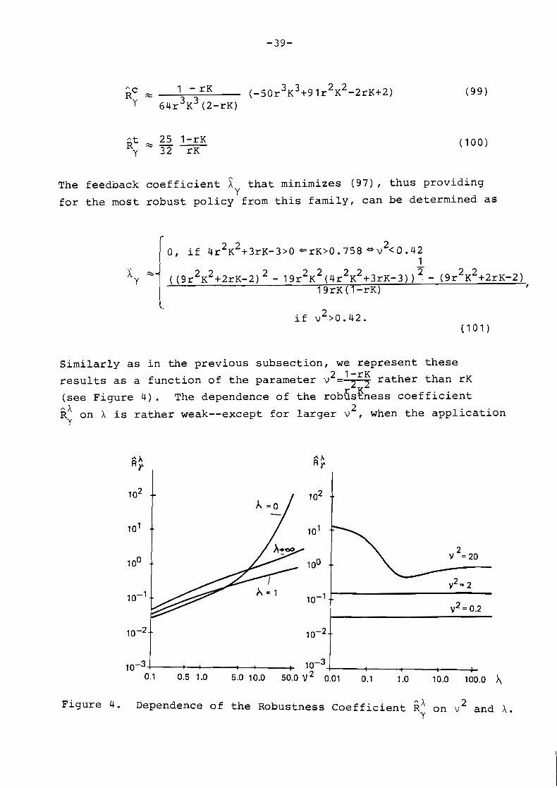
Similarly as in the previous subsection, we represent these - - -

l-rK rather than rK results as a function of the parameter v =-

(see Figure 4). The dependence of the robgskess coefficient ..A R on h is rather weak--except for larger v2, when the application

Y

^ A Figure 4. Dependence of the Robustness coefficient R on v2 and A. Y

of X 4 ^X is not advisable. Y

A A

However, since h > A (see Figure 4a) and Rh does not rise A B Y Y

steeply for X > X - , , we may. presume that the feedback coefficient X 'I

should be chosen to i to provide for greater robustness with B

respect to the uncertainty about natural unemployment rate than

with respect to the uncertainty about the functional form of the

Phillips curve. A A

A simplified form for a compromise X (that is close to X A A A 13

but satisfies X < X < A ) can be obtained by assuming Y B

A

(see Figure 5a). If this particular X is chosen, then the A CK A CK policy target Q(t,a)-A - - Si(t, a)= u(t)- X - x(t) can be

q - q

A A

Figuse 5. a) Comparison of Optimal Feedback Coefficients X A , and X 6'

Y' A A

A

b) Comparison of Robustness Coefficients f ih and R at h=h and of the Relative Speed u/r of Controlling 1nflition ~Zwards Its Long- term Value.

transformed to the form

where

This means that a robust policy is to choose money supply

rate m as to keep the combination of unemployment and the ex- C pected inflation, u(t)- -x(t), at the predeter~ined tgajectory

C r q A X E (un- - xO) e-Ut. The robustness coefficients Rh and R corres-

r q B 2 y ponding to this policy are shown as functions of v in Figure 5b;

u parallel to this, Figure 5b also displays the coefficient 7 -- the relative speed of controlling inflation towards its long-

term value--from Figure 1.

The graphs in Figure 4b should be interpreted as follows.

Once a coefficient X and thus a robust policy form has been

chosen, the robustness coefficients depend on basic parameters

of the model. The aggregate parameter v2 can be inversely in-

fluenced by the choice of weighting coefficient q at the un-

employment rate u (t) in the social welfare functional (1 0) . If

this coefficient is large enough, such that the resulting v2 is

small, say, vL<2, - then the attainable robustness coefficients CI

are quite good. However, for vL<2 - we have the relative speed

u/r<l, - which means that we control inflation slower than the

time discount rate--a solution that is socially not acceptable. 2 To increase the relative speed, we must go to v >2; at v2=20

we obtain u/r=4, which with r=O.l/year would give u=0.4/yearI

still a moderate speed of controlling inflation (a reduction of

circa 40% of the original distance x0-Bm in a year). However,

the robustness of the solution suffers from the choice of the

higher relative speed. If some impetous decision-maker would

promise his electorate to bring the inflation down in a year

(say to. achieve u/ralO) he would have to go as far as to v2a100,

where the robustness coefficients are rather bad; errors in model

specification might then easily result in social welfare losses

several times higher than the social welfare losses due to the

initial difference xo-2,

Admittedly, the results shown in Figure 5b are based on the

assumed bounds 161max and IyImax. While these bounds do not in-

fluence the conclusions on the choice of the feedback parameter

A , they do influence the actual values of robustness coefficients.

Thus, an impetous decision-maker could require more precise

econometric estimations of the bounds on parameter uncertainty.

Our theoretical exercise does not permit us to draw conclusions

about the desirable degree of accuracy for parameter evaluations;

it provides only possible guidelines for the econometric pursuit

of such conclusions. However, given an attainable degree of

accuracy, the results will have the same qualitative character:

the faster we try to achieve the long-term goals, the more sen-

sitive to model errors are the results of our policy.

For the sake of brevity, we omit here the discussion of

Hamiltonian-maximizing and benefit-to-cost maximizing policies,

although the former policies might make sense in the case of a

mistaken functional speicification.

5d. Sensitivity to Delays

We assume here - a=(O,0,~), that is, the extended model takes

the form

x(0) =xo , u(t) - given for t€[-r;O) (105)

The problem of maximizing (10) subject to (105) is, in fact, not

very difficult to solve (see the appendix). However, this is

due to the special form of the problem and we shall proceed as

if we did not know its explicit solutions. We can do so, be-

cause we know its solutions if T=O (the basic model solutions)

and we need only linear approximations of its solutions for

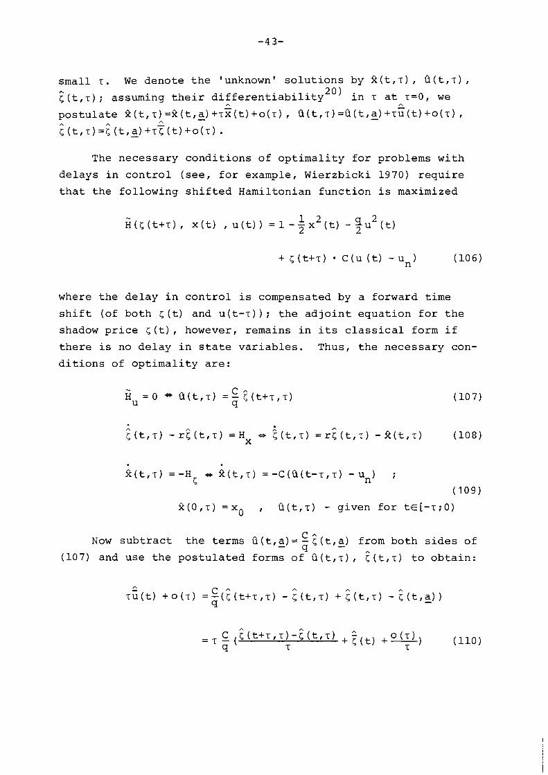
smal l T . We denote t h e 'unknown' s o l u t i o n s by f ( t , ~ ) , Q ( ~ , T ) , h

5 (t , T ) ; assuming t h e i r d i f f e r e n t i a b i l i t y A

2 0 ) i n T a t A T = O , we

p o s t u l a t e 2 ( t , ~ ) A = f ( t , a ) + ~ x ( t ) + o ( ~ ) - Q ( ~ , T ) = a ( t , a ) + ~ u ( t ) + o ( ~ ) - , A

5 ( t , ~ ) = ; ( t , a ) + ~ T ( t ) + o ( ~ ) . -

The necessary cond i t i ons of o p t i m a l i t y f o r problems wi th

de lays i n c o n t r o l ( s e e , f o r example, Wierzbicki 1970) r e q u i r e

t h a t t h e fo l lowing s h i f t e d Hamiltonian func t ion i s maximized

where t h e de lay i n c o n t r o l i s compensated by a forward t ime

s h i f t (of both 5 (t) and u ( t - T ) ) ; t h e a d j o i n t equat ion f o r t h e

shadow p r i c e ~ ( t ) , however, remains i n i t s c l a s s i c a l form i f

t h e r e i s no de lay i n s t a t e v a r i a b l e s . Thus, t h e necessary con-

d i t i o n s of o p t i m a l i t y a r e :

2 ( 0 . r ) = x g , Q ( t , r ) - given f o r t ~ [ - r ; O )

C Now s u b t r a c t t h e terms Q ( t , a ) = - 5 ( t , a ) from both s i d e s of - 9: -

(107) and use t h e p o s t u l a t e d forms of Q ( ~ , T ) , % ( t , ~ ) t o ob ta in :

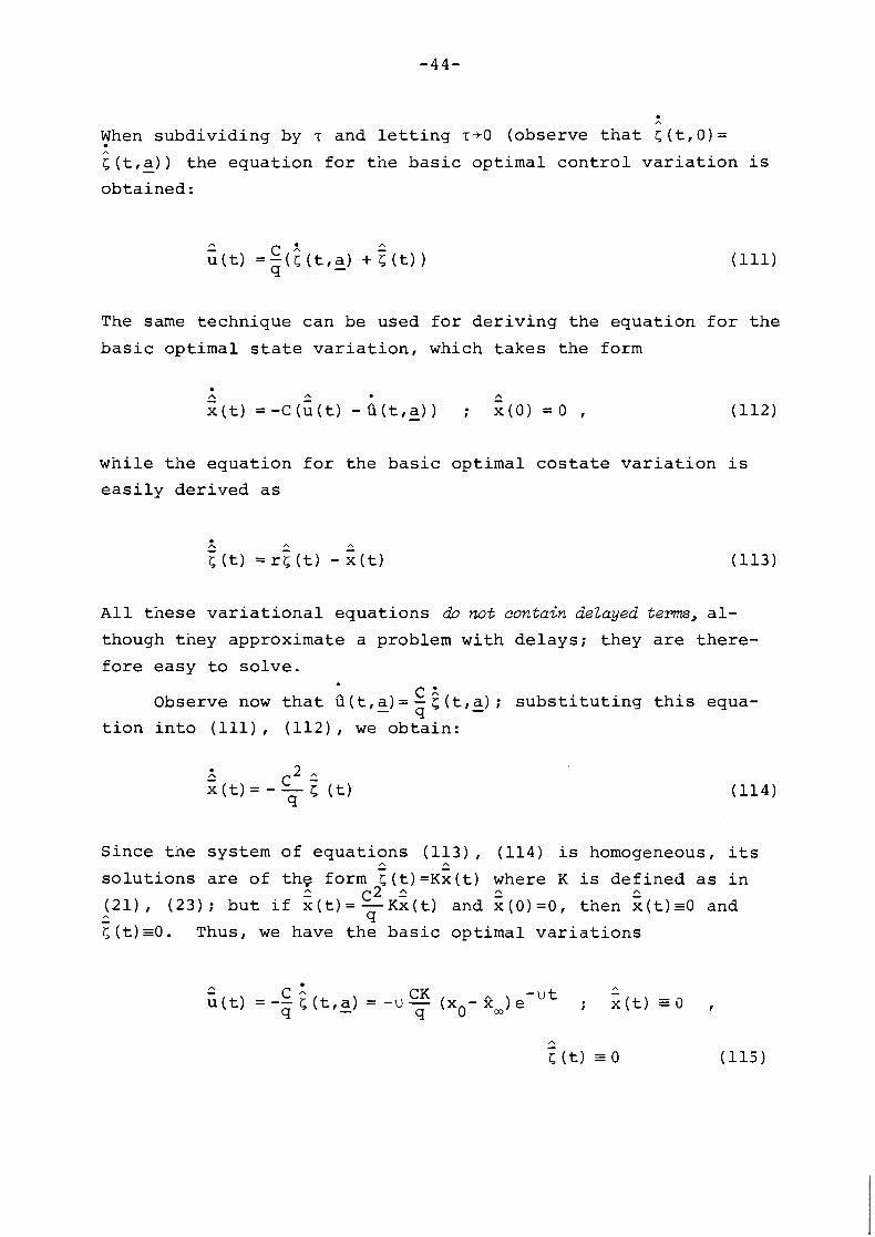
A

When subdiv id ing by T and l e t t i n g T+O (observe t h a t < ( t , O ) = A

< ( t , a ) ) - t h e equat ion f o r t h e b a s i c opt imal c o n t r o l v a r i a t i o n i s

obta ined:

The same technique can be used f o r d e r i v i n g t h e equat ion f o r t h e

b a s i c opt imal s t a t e v a r i a t i o n , which takes t h e form

whi le t h e equat ion f o r t h e b a s i c opt imal c o s t a t e v a r i a t i o n i s

e a s i l y der ived a s

. A - A A

< (t) = rt (t) - ;; (t)

A l l t h e s e v a r i a t i o n a l equat ions do not contain delayed terms, a l -

though they approximate a problem wi th de lays ; they a r e the re -

f o r e easy t o so lve .

C =. Observe now t h a t C i ( t , a ) = - s ( t , a ) ; - s u b s t i t u t i n g t h i s equa- q

t i o n i n t o ( I l l ) , ( 1 1 2 ) , we ob ta in :

S ince t h e system of equat ions (113 ) , ( 1 1 4 ) i s homogeneous, i t s , , , ,

s o l u t i o n s a r e of t h e form t ( t ) = ~ x ( t ) where K i s de f ined a s i n A c2 A

A A

( 2 1 ) . ( 2 3 ) ; b u t i f x ( t ) = ; ; ~x ( t ) and ~ ( o ) = o , then x ( t ) = 0 and A - 7

< ( t ) - 0 . Thus, we have t h e b a s i c opt imal v a r i a t i o n s

A - < (t) = 0

Consider now t h e fami ly ( 4 1 ) of c losed- loop p o l i c i e s . The

extended model equa t i on under t h e s e p o l i c i e s t a k e s t h e form:

X x (t) - given by (105) f o r ~ € [ O ; T ] ( 1 1 6

Provided that the equatwn (116) i s stable, w e can approximate i t s

s o l u t i o n a s a d i f f e r e n t i a b l e f unc t i on of t i m e . ay s u b t r a c t i n g t h e b a s i c model equa t i on from both s i d e s of ( 1 1 6 ) , subd iv id ing

by T and l e t t i n g r+O, w e o b t a i n t h e equat ion f o r b a s i c s t r u c t u r -

a l v a r i a t i o n s

which y i e l d s t h e s o l u t i o n

and whi le t ak ing i n t o account ( 4 1 )

- A CK - X CK u-(xo - A _ ) (e -"t - u t (119) u ( t) =A-x ( t) =_- q X l q - e 1

Thus, t h e extended s t r u c t u r a l v a r i a t i o n s a r e

- X A - A - u x ( t) = x ( t) - x ( t ) = -(x - krn) (e - h u t - . -u t ) A - 1 0 ( 1 2 0 )

and t h e second-order d e r i v a t i v e of t h e we l fa re l o s s i s d e t e r -

mined a s

2 s A T ^ A max T T - R = - ( 1 - r K )

n2k 4 (rK+2A ( 1 - r K ) )

Observe t h a t t h i s r obus tness c o e f f i c i e n t dec reases monoton ica l ly A

w i t h A . Hoyever, i f w e assume A = A , w e o b t a i n r e l a t i v e l y sma l l

v a l u e s o f kA a s shown i n F igu re 6 . r

^ A ^ A F igure 6 . Comparison o f Robustness C o e f f i c i e n t s R R and &: wi th A = X . B ' T I

Thus, w e can conclude t h a t the omission of delays in the basic

mdel does not jeopardise the successful application of closed-loop po licies

to the extended model with delays--provided t h a t t h e ex tended model

remains s t a b l e and t h e approximat ion of t h e we l f a re l o s s remains ^ A v a l i d (observe t h a t a c o r r e c t l y computed STT would i n c r e a s e

s h a r p l y , even t o i n f i n i t y , i f t h e extended model becomes un-

s t a b l e ) .

Therefore, we must investigate stability conditions of the

equation (116). Since this equation is linear, it is sufficient

to analyse the stability of its homogeneous part:

P(t) = -hux(t-r) ; x(t) = 0 for t < 0 , x(0) =xo (123)

When applying Laplace transformation to both sides of this equa-

tion, we obtain

and we can use (see the appendix) the classical Nyquist crite-

rion for the stability of a feedback system. The result is that

the equation (116) is stable, if

(where ~=3.14 ...). Therefore, the use of a sufficiently large

feedback coefficient X would destroy the stability of the system.

Moreover, it is known from the classical theory of feedback

systems, that the condition (125) should be satisfied with 50%

margin Tr

TU < - 4X (126)

in order to obtain approximately aperiodic solutions of (116), A which is necessary for a satisfactory approximation of x (t) by

2(t,a)+rxX - (t) , since both B(t,a) - and G' (t) are aperiodic.

We can investigate further the condition (125) if we assume A

X=X, consider as a function (102) of v, i ( v ) = 2v2 2 1 I

1 2 - ( 1 + 4 ~ ) 2 - 1 U consider - as a function of v, - - r - ) , and transform the

r 2 condition (125) to

or, if taken with 50% margin

Since r and r might be taken as given parameters--say,

r=O.l/year and r=0.25 years as an estimate of delay21--hence the

inequality (128) specifies really the highest value of the param-

eter v2 that is admissible for a stable implementation of the

closed-loop policy (41) with x=X. For example, if r=O.l/year

and r=0.25 years, we obtain vL<31.4, ., 'max

=rmv<0.560/year. If I

'max =C/qz is higher than this value--say, because of a very small

weight q related to the unemployment in the social welfare func- A

tional--then the closed-loop policy with X=X is not desirable.

However, for these high values of v2 all other policies are also

very sensitive to all types of errors (see Figures 3, 4, 5).

Thus, if the weight q is small, resulting in relative high speed

u of controlling inflation or, equivalently, in a hight value of 2

the parameter v , a monetary control of inflation and unemploy-

ment cannot really be effective--either because of delayed

effects endangering stability or because of incomplete informa-

tion and various modeling errors.

On the other hand, u, u and v2 can always be diminished max

by increasing the weight q related to the unemployment. After

all, a relative speed of u =0.56/yearf u=0.5l/year is not that -0.51 max

small: e %0.60, which means that the long-term solution is

being approached at a rate of circa 40% per year. In short,

these results suggest that policy directions aimed at achieving

the long-run target rates of inflation and unemployment rapidly

run the risk of either inducing instability or becoming partic-

ularly sensitive to unpredictable modeling errors. Policy

directions which aim for a slow, gradual achievement of the long-

run targets have a greater chance of success.

6. OVERVIEW

In the analysis above we have presented a methodology for

the formulation and assessment of macroeconomic policy rules

under conditions of uncertainty or simplistic modeling. We

believe that these conditions are prevalent in macroeconomic

policy making: rarely do policy makers have accurate knowledge

of the parameter distributions in their models and usually these

models are recognized as rough approximations of the macroeco-

nomic phenomena which the policy makers face. The policy maker

is assumed to know which parts of his macro-economic model may

be subject to error--which parameter estimates and delay esti-

mates may be mistaken and which functions may be misspecified--

but he does not know how these errors are distributed.

In this setting, the policy maker formulates a number of

different policies each of which optimize his objective function

(viz., the "social welfare function") subject to the constraints

represented in his model. The policy which is actually chosen

is the one which makes social welfare minimally sensitive to the

given modeling errors. This is not a narrowly prescribed, water-

tight exercise, because the number of policies to choose from is

limited only by the policy maker's imagination. Our methodology

does not reduce the policy maker to a spiritless automaton

which solves a given optimization program over and over again.

The policy maker always faces the possibility of discovering

new policy options which may make social welfare even less sen-

sitive to his modeling errors than the policies he currently

employs. It does not appear possible to find a universally

"best" policy with regard to our methodology. All that our

methodology does is provide criteria for the choice of a policy

from a given set of candidate policies.

Tne traditional way of deriving how sensitive social wel-

fare is to policies derived from modeling errors is (a) to maxi-

mize social welfare with respect to the "wrong" model and there-

by derive the "wrong" policy, (b) to maximize social welfare

with respect to a hypothetically "right" model and thereby de-

rive the "right" policy, (c) to find the level of social welfare

associated with the "right" model and the "wrong" policy, and

(d ) t o take t h e d i f f e r e n c e between s o c i a l we l fa re under (b ) and

( c ) . I n ou r methodalogy, we e s s e n t i a l l y fo l low t h i s way. How-

eve r , we change t h e i n t e r p r e t a t i o n of t h e ' r i g h t ' and 'wrong'

models by rep lac ing them wi th 'extended' and ' b a s i c ' models,

and w e s imp l i f y t h e s t e p s (b , c , d) by model l i n e a r i z a t i o n . The

extended model i s n o t ' r i g h t ' , t h e b a s i c model i s n o t 'wrong1--

f o r i f t h e po l i cy maker w e r e a b l e t o f i n d t h e s o c i a l l y opt imal

po l i cy w i t h regard t o t h e ' r i g h t ' model, t h e r e would be no rea-

son f o r him t o use t h e 'wrong' model i n t h e f i r s t p lace . Thus,

t h e b a s i c ( n o t 'wrong') model i s r e a l l y , f o r a g iven purpose,

t h e b e s t r e p r e s e n t a t i o n of t h e problem a t hand, and t h e extended

(no t ' r i g h t ' ) model s imu la tes poss ib le , n o t a c t u a l e r r o r s i n t h e

b a s i c model. Moreover, when apply ing our methodology, w e do n o t

have t o so l ve t h e more complicated extended model--neither t o

opt imize it e x a c t l y , nor t o determine e x a c t l y t h e impact of t h e

basic-opt imal ( n o t 'wrong') po l i cy i n t h i s model. I ns tead of

t h i s , w e apply l i n e a r approximations t o t h e extended model so lu-

t i o n s i n both c a s e s , and approximate thus t h e s o c i a l we l fa re

l o s s a s requ i red i n t h e s t e p ( d ) . Our methodology permi ts t hus

t h e po l i cy maker t o choose a robus t po l i cy ( v i z . , from a given

set of cand ida te p o l i c i e s , t h e one t h a t makes t h e s o c i a l we l fa re

l e a s t s e n s i t i v e t o modeling e r r o r s ) wi thout r e q u i r i n g t h a t t h e

s o c i a l we l fa re op t im iza t i on problem be so lved wi th re fe rence t o

t h e more compl icated, extended model.

Our methodology a p p l i e s t o a l l macroeconomic problems i n

which p o l i c i e s a f f e c t s o c i a l we l fa re a t p r e s e n t and i n t h e f u t u r e

and t h e r e i s a t radeo f f between these we l fa re e f f e c t s . A s noted

i n Sec t ion 1, a l a r g e number of macro-economic problems sha re

t h e s e p r o p e r t i e s . The problem of i n f l a t i o n and unemployment

which w e chose t o ana lyse performs simply an i l l u s t r a t i v e pur-

pose. I n f a c t , t h e r e i s no reason why ou r methodology should be

app l i ed s o l e l y t o macro problems. Microeconomic problems w i th

t h e p r o p e r t i e s above--say, a f i r m maximizing t h e d iscounted

s t ream of i t s p r e s e n t and f u t u r e p r o f i t s s u b j e c t t o unce r ta in

techno log ica l condi t ions- -are usua l l y amenable.

Yet, w i th in t h e con f ines of t h e p a r t i c u l a r problem of in -

f l a t i o n and unemployment t r e a t e d i n t h i s paper , we examined t h e

mone ta r i s t case f o r c o n s t a n t money growth r u l e s and developed a

r a t h e r s c e p t i c a l s t a n c e i n t h i s regard . Furthermore, w e w e r e

a b l e t o fo rmu la te a r i g o r o u s argument a g a i n s t " impetuous" p o l i c y

making ( i . e . , p o l i c i e s which cause t a r g e t v a r i a b l e s t o approach

t h e i r long-run op t ima l l e v e l s r a p i d l y ) . Such a p o l i c y s t r a t e g y

may induce i n s t a b i l i t y , e i t h e r through de lay e f f e c t s , o r by mak-

i ng t h e nacroeconomic system very s e n s i t i v e t o modeling e r r o r s .

Although one cou ld s u s p e c t t h a t such a conc lus ion i s val id--by

comparing, s a y , t h e e f f e c t s o f i n f l a t i o n and unemployment

p o l i c i e s i n c o u n t r i e s such a s A u s t r i a and t h e USA o r Grea t

Br i ta in - -a r i g o r o u s argument us ing model u n c e r t a i n t y and p o l i c y

robus tness c o n s i d e r a t i o n s adds t o a f u r t h e r unders tand ing o f

t h i s problem.

APPENDIX: MATHEMATICAL DERIVATIONS

SoZutwn o f the Basic Mode2

For the problem:

1 2 2 maximize W(x,u) = (1 - x (t) - 9 u (t) ) dt 2 (All

X I U

subject to differential constraint--the state equation:

we have the (current value) Hamiltonian function:

and first-order optimality conditions

together with the state equation (A2). We do not know yet

whether a s o l u t i o n of t h e problem ( A l ) , ( A 2 ) e x i s t s . However,

i f we s u b s t i t u t e ( A 4 ) i n t o (A2 ) and combine wi th (A5) , we o b t a i n

t h e system of canon ica l equat ions :

which can be so lved by us ing t h e R i c c a t i s u b s t i t u t i o n :

where K ( t ) and M ( t ) a r e supposed t o be such t h a t (A7) ho lds in -

dependent ly of xo. By s u b s t i t u t i n g (A7) i n t o t h e second equa-

t i o n i n (A6) whi le t a k i n g i n t o account t h e f i r s t one, we o b t a i n

o r , equ iva len t l y

S ince t h i s equat ion should hold independent ly of xo , t h u s , a l s o

of x ( t ) , both of i t s s i d e s must be zero. I n t h i s way, w e der ived

t h e R i c c a t i equat ion:

(t) + r K ( t ) - 1

and t h e a u x i l i a r y equat ion

These e q u a t i o n s a r e u s e f u l f o r many a s p e c t s o f a n a l y s i s of

op t ima l s o l u t i o n s of t h e problem ( A l ) , (A2) : n o t o n l y t hey de-

f i n e c losed- loop c o n t r o l laws and t h e second-order d e r i v a t i v e

K ( t ) of t h e ( c u r r e n t va lue ) Bellman op t ima l v a l u e f u n c t i o n , b u t

a l s o t hey can be used t o check s u f f i c i e n t c o n d i t i o n s f o r o p t i -

m a l i t y . One o f t h e v a r i o u s forms o f s u f f i c i e n t c o n d i t i o n s of

t h e e x i s t e n c e and o p t i m a l i t y o f s o l u t i o n s t o ( A l ) , (A2) i s a s

f o l l ows (see, f o r example, Wie rzb ick i 1977 ) :

1) The s o l u t i o n s shou ld s a t i s f y t h e necessa ry c o n d i t i o n s

(A41 (A51 (A21 - 2) Tne second-order d e r i v a t i v e H o f t h e Hami l ton ian uu

f u n c t i o n (A3) shou ld be s t r i c t l y n e g a t i v e f o r a l l t

(which i s , indeed , t h e c a s e ) . 3) The R i c c a t i e q u a t i o n s ( A l O ) , ( A l l ) shou ld p o s s e s s

bounded s o l u t i o n s when so l ved backward i n time--which,

i n t h e c a s e of c o n s t a n t c o e f f i c i e n t s and an i n f i n i t e

t i m e i n t e r v a l , means t h a t t hey shou ld have a s t a t i o n a r y

s o l u t i o n t h a t i s s t a b l e backwards i n t i m e .

The l a s t two c o n d i t i o n s a r e s u f f i c i e n t f o r s t r i c t n e g a t i v e

d e f i n i t e n e s s of t h e Hess ian o p e r a t o r of t h e w e l f a r e f u n c t i o n a l

reduced t o t h e space of c o n t r o l t r a j e c t o r i e s . Now, t h e s t a t i o n -

a r y s o l u t i o n s o f t h e R i c c a t i equa t i on (A10) r e s u l t from t h e

f o l l ow ing e q u a t i o n

and have t h e form

Of t h e s e two s o l u t i o n s , on ly t h e p o s i t i v e one is backward-

s t a b l e . W e can check t h i s by app l y i ng t h e f i r s t Lapunov theo-

r e m : a s o l u t i o n o f a n o n l i n e a r d i f f e r e n t i a l equa t i on i s asymp-

t o t i c a l l y s t a b l e , i f a l i n e a r i z e d e q u a t i o n a t t h i s s o l u t i o n is

a s y m p t o t i c a l l y s t a b l e , and u n s t a b l e , i f t h e l i n e a r i z e d e q u a t i o n

is unstable. To check backward-stability, we change the sign of

time, and linearize (A10) at K(t)=K to obtain

where k(t) is a variation of K(t). This equation is asymptoti- 2c2

cally stable if - 2c2 K + r > O ; b u t - K + r=-+- q 9

C2K from (A12) , K q

hence we must have K>O. Hence, the backward stable stationary

solution of (A10) is

c2 (where we introduced a composite parameter v2 =- 2 , for reasons

explained in the main text in the paper). The gqgation (All)

has a stationary solution

c2 1 which is backward-stable if -K+ r=->O, hence if K>O. q K

We can now substitute the values of K and M into (A7) , (A6)

to obtain

c2 2 Since Cu - -M=Cun(l-- K ) = rKCu the integration of (Al7) n q q n '

yields

c2 rKCun rqun where u = - K; if we denote - -- u C by f im, then

q

By s u b s t i t u t i n g t h i s i n t o (A7) w e o b t a i n

rKqun where e , = ~ 8 ~ + ~ = + C U , K ~ = T ( r K q"n + - ) =- C ~ K ~ qun

9 C ' By s u b s t i t u t i n g t h i s i n t o ( A 4 ) , w e o b t a i n

Now, t h e s o l u t i o n s (A19), (A20), (A21) a r e indeed t h e so lu -

t i o n s of t h e problem ( A l ) , (A2), s i n c e t h e y s a t i s f y t h e f i r s t -

o r d e r necessary c o n d i t i o n s and they cor respond t o a backward

s t a b l e s o l u t i o n o f t h e R i c c a t i equa t i on , wh i le t h e second d e r i -

v a t i v e o f t h e Hami l tonian f u n c t i o n t h e r e i s s t r i c t l y n e g a t i v e

( t h u s , t h e w e l f a r e f u n c t i o n a l W , t r e a t e d a s a f u n c t i o n a l o f

c o n t r o l t r a j e c t o r y u a l o n e , wh i l e t h e dependence on s t a t e t r a -

j e c t o r y x i s reduced by s o l v i n g t h e s t a t e equa t i on (A2) and sub-

s t i t u t i n g i n t o ( A l ) , has i t s second-order de r i va t i ve - - t he

Hessian o p e r a t o r - - s t r i c t l y nega t i ve d e f i n i t e ; t h i s i s s u f f i c i e n t

f o r t h e e x i s t e n c e of a unique maximum o f t h e we l f a re f u n c t i o n a l .

The c o n t r o l t r a j e c t o r y u i s h e r e cons idered t o be an e lement o f -rt 2 1 a H i l b e r t space w i t h t h e norm I 1 u 1 1 = ( Sme u (t) d t ) 1)) .

0 When ana l ys ing t h e ob ta ined op t ima l s o l u t i o n s , w e observe

t h a t t ney depend a c t u a l l y on t h r e e parameters . These paramete rs

a r e : t h e d i s c o u n t r a t e r; t h e n a t u r a l unemployment r a t e un; and c2 t h e composi te parameter v 2 = - 2 t h a t , a t g i ven r , cou ld be t aken r q

a s r e p r e s e n t i n g t h e i n f l u e n c e of t h e weight ing c o e f f i c i e n t q and

t h e squared c o e f f i c i e n t C L .

Thus, t h e R i c c a t i c o e f f i c i e n t K , d e f i n e d by ( A 1 4 ) , depends 2 on r and v , wh i l e r K depends on v 2 a lone . A t a g iven va lue o f

r , K dec reases monoton ica l ly a s a f u n c t i o n o f v 2 from t h e va lue 1 - a t v+O ( say , q+m) t o 0 a s v + m ( say , q+O). On t h e o t h e r hand, r a s a f u n c t i o n of r , t a k i n g i n t o account t h e dependence o f v 2

on r ( a t g i ven C,q) K a l s o d e c r e a s e s monoton ica l ly

from t h e va lue g a t r-0 t o 0 a s r-a (we could s e t K = l / r f o r L 2 2

l a r g e enough r such t h a t r > > 4 C / q ) . The r e l a t i v e speed co-

e f f i c i e n t u has t h e form:

Thus, i f r i s given, u i nc reases monotonical ly a s a func t i on of

v 2 from t h e va lue 0 a t v=O (say , q-a) t o a a s v-a (q-0; we could

set u w v f o r v > > 1 / 2 ) . This means t h a t i nc reas ing t h e weight q

t o unemployment n e c e s s a r i l y decreases t h e r e l a t i v e speed of

con t ro l . On t h e o t h e r hand, a s a func t ion of r a t g iven C,q,

t h e speed c o e f f i c i e n t u decreases monotonical ly , from t h e va lue

c2 1 a t r = O , t o t h e va lue 0 a s r- ( w e could set u-- f o r r > > 2 ~ / q q ) .

q r Thus, a l a r g e r d i scoun t r a t e a l s o decreases t h e r e l a t i v e speed

of con t ro l .

However, i f w e assume t h a t it i s s o c i a l l y d e s i r a b l e t o have

t h e r e l a t i v e speed c o e f f i c i e n t u a t l e a s t a s l a r g e a s t h e d i s -

count r a t e r , u / r > l , - then w e e a s i l y o b t a i n from ( A 2 2 ) t h a t t h i s 2 could happen on ly i f v - > 2 --and, from ( A 1 4 ) t h a t t h i s co r res -

ponds t o KL . 2 For t h i s range of v > 2 ( v > > 1 / 2 ) w e can set - L ' M V = - = u 1 max1 thus u p r a c t i c a l l y does no t depend on r and

9 2 changes only w i th C and q , decreas ing w i th an inc reased q.

The opt imal va lue of t h e s o c i a l we l fa re func t i on , a f t e r

app rop r ia te i n t e g r a t i o n s (omi t ted here) has t h e form

Observe t h a t t h i s i s a q u a d r a t i c f unc t i on of x a , w i t h

and

Thus, t h e c o s t a t e v a r i a b l e determines t h e f i r s t d e r i v a t i v e

of t h e op t ima l v a l u e f u n c t i o n , wh i l e t h e R i c c a t i c o e f f i c i e n t - -

i t s second-order d e r i v a t i v e . These a r e known p r o p e r t i e s o f t h o s e

v a r i a b l e s , and a r e p resen ted h e r e on l y i n o r d e r t o check t h e

c o r r e c t n e s s of a r a t h e r long i n t e g r a t i o n i n (A25). The forms 2..

AW and A W r e p r e s e n t t h e f i r s t and second-order p a r t s o f w e l f a r e

l o s s e s due t o t h e i n i t i a l d i s e q u i l i b r i u m x0-9,.

F i n a l l y , observe t h a t w e can r e p r e s e n t t h e op t ima l c o n t r o l

B ( t ) a s a f u n c t i o n o f 2 ( t ) and n o t a s a f u n c t i o n o f xo:

which g i v e s t h e c l a s s i c a l v e r s i o n o f t h e c losed- loop op t ima l c o n t r o l . CK U

The feedback c o e f f i c i e n t - = - has t h e sane p r o p e r t i e s a s t h e r e l a - q c

t i v e speed c o e f f i c i e n t u , s c a l e d down by C. Thus, f o r u / r > l , - 2 v >2, w e have -=--- - CK - Th is has an impor tan t i n t e r p r e t a -

9 C 1' qT

U t i o n : s i n c e G ( t ) - u = - ( 2 ( t ) - f i m ) , hence a t op t ima l s o l u t i o n s , t h e n 0 r a t i o o f t h e (out -o f -equ i l ib r ium) unemployment Ci( t)-u t o t h e

n (ou t -o f -equ i l i b r ium) expec ted i n f l a t i o n B( t ) -P, approaches, b u t

1 never exceeds, t h e v a l u e l/qT.

Bounds on Parameter Chaxges

In this theoretical exercise, bounds on parameter changes

must be assumed heuristically, however, with some rational argu-

ments. We observe that first 8_ = 7 un . If we are uncertain - about the actual natural rate of unemployment, un, the largest

mistake we can reasonably postulate is related to the assumption

that the current expected inflation x is equal to its long-term - C 0 optimal value, x == G

.., u =- C B=u -u =- 0 C n' n rq X ~ '

X -u = n n r q O n

C rq(~O-2,) Such a mistake is not very probable: observing a

real economic process, we can usually tell whether we are far or

close to the long-term equilibrium. Thus, we assume that we can

estimate at least half of the distance from the long-term equi-

librium, whicn gives half as large bound on the uncertainty

parameter B:

To obtain a comparable bound on the parameter y, we assume

that we observe correctly the variable

x-xa - -- A = u-G - $(u-Gn) 2 A n

A-u+Gn which would give y=2 2 ' We are uncertain about both

(u-an)

L A-u+G and (u-Gn) . We can assume 1 A-u+G 1 < I B I n n max since this

uncertainty is related to the uncertainty in Gn. However, the

larger is (u-G ) 2, the better conclusions we can obtain about n

y; in a probabilistic estimation, this fact would correspond

to the impact of the variance of the explaining variable. Thus,

we must assume some minimal ' variance ' (u-Gn) ; if we take, 2 2 arbitrarily, a rather small 'variance' (u-Bn) =4un, then we

obtain the bound

TO o b t a i n a bound on t h e maximal neg lec ted de lay T~~~ w e

n o t e t n a t i f t h e - p o s t u l a t e d op t ima l change of t h e expec ted i n f l a -

t i o n has t h e form S ( t ) = (xo-kw) e - U t + ~ , and a r e a l economic pro-

c e s s would e x h i b i t a de lay T i n t h e impact o f unemployment on i n -

f l a t i o n , w e would observe a c t u a l % ( t ) = x f o r t < ~ . Thus, t h e 0 -

observed d i f f e r e n c e has t h e form:

i ( t ) - 9 (t) = (xo-ltw) (l-e-Ut) , (xo-9_) u t , t < ~ - (A31)

Now w e assume a r b i t r a r i l y t h a t w e might over look t h i s d i f -

f e r e n c e u n t i l i t s r e l a t i v e va lue becomes 2 5 % , t h a t i s , u n t i l

- - ( ) - Thus, t h e maximal de lay t h a t we can over look i s X - 4 '

bouidea by

(he re w e assume t h a t w e a r e i n t e r e s t e d i n t h e range o f s o l u t i o n s 2

where u / r > l , - v - > 2, and u umax) .

Sens i t iv i ty t o Errors i n Estimating Natural Unemployment Rate

I n t n i s c a s e , w e assume t h a t p o l i c i e s de r i ved from t h e

~ a s i c model w i t h parameter u a r e a p p l i e d t o an ex tended model, n which d i f f e r s from t h e b a s i c one on ly by a changed parameter Gn,

where ii -u =f3; t h e parameter a= ( f3,0,0) , t h e parameter a= (0 , O , 0 ) . n n - - Hence, i n t h i s s imp le c a s e w e know t h e op t ima l s o l u t i o n s f o r t h e

extended model which w i l l be denoted h e r e by k ( t , a ) = x ( t , f 3 ) , - Q (t ,g) =Q ( t , 8 ) ; i n p a r t i c u l a r

I f w e s u b t r a c t from t h e s e s o l u t i o n s t h e s o l u t i o n s (A18), ( A 2 1 )

f o r t h e bas i c model--denoted he re by 2 ( t , a ) - , Q(t , a ) - --we o b t a i n

A n - By t h e d e f i n i t i o n of b a s i c opt imal v a r i a t i o n s x ( t ) , u ( t ) --

see Equation (56)--we o b t a i n i n t h i s case

Now w e cons ider t h e fami ly of closed-loop c o n t r o l p o l i c i e s :

and suppose such a po l i cy i s implemented t o t h e extended model

wi th finfun; w e denote t h e s t a t e and c o n t r o l under such implemen- A A t a t i o n by x (t) , u (t) :

A CK A A (t) = - C ( Q ( t , a ) - -Gn+A (X t - t ;

Now, l t ( t , a ) - s a t i s f i e s l t ( t , a ) =-C ( G ( t , a ) - -un) ; by s u b t r a c t i n g t h i s

from both s i d e s of Equation (A38), w e o b t a i n

A A A ( t) - f t ( t , a ) - =-Au(x (t) - 2 ( t , g ) ) +CP ;

2 where u= - and 8=Bn-un. The s o l u t i o n of t h i s equat ion i s

q

which, when set into (A37), yields

Thus, the basic structural variations--see Equation (54)--we

have the form

and the extended structural variation--see Equation (55)--are

A 1 2 (t) = % (- (l-e-"Jt C ArK - (~-e-'~)) ;

aA(t) = r ~ e -ut-e-Aut

To compute the second-order derivative g A of the welfare B B losses--see Equation (53)--we have to integrate the expression

which after rather long integrations and transformations (omitted

here for brevity's sake; however, these transformations have been

checked by assuming A=0,1, or and performing independent,

simpler integrations and transformations) results in

Now, the robustness coefficient &A = g A / c% is easily B B B determined

aiiA The equation A= 0 is a quadratic equation in A (with the a h

full form omitted for the sake of brevity); we choose by check- a2ffb

iny the sign of - ..A the root that indeed minimizes R a h 2 B :

While taking into account that rK = (1+4vL) - 1 is a mono- 2v 2

2 tonically decreasing function of v2, with rK-1 as v -0, we can A

show that X is a monotonically decreasing function of rK and B A 2 thus increasing function of v2, with X -1.5 as v -0. The graphs B

of 1 and 6' are given in Figures 3, 5 in the main text. B B The open and the closed-loop Hamiltonian maximizing policies

as well as the open and closed-loop benefit-to-cost maximizing

policies are considered in the main text.

Here we show only that the welfare losses under the open-

loop benefit-to-cost maximizing policy are larger than the cor-

responding welfare losses under the open-loop policy. With this

aim, we recall Equation (78) for the extended structural varia-

tions :

where

Since t h e s t r u c t u r a l v a r i a t i o n s under t h e open-loop po l i cy

have t h e form (see Equation (A43), where we should s e t X = O ) :

- u t g O ( t ) = C t - F ( l - e ) > 0 ; Go ( t) = rKe -u t - 1 < 0

- f o - f o and do no t depend on xo , when computing x ( t) , u ( t) we can

assume any reasonable xo t h a t does no t i n c r e a s e t h e s e v a r i a t i o n s

unnecessar i l y . The most reasonable assumption i s x,=8-, which V -

means t h a t we w i l l compute k f O ( t ) , c f0 ( t ) along t h e long-term

equ i l ib r ium f o r t h e b a s i c model. I n such a case , we o b t a i n

q f o = 1 - rite - u t f o c - u t + K (F + rqC(1-e ) )

Observe t h a t f o r reasonable va lues of q , u v 2 we have -0

n' ~ ( 8 , G , a ) = l a n d - r fo << r / C , qfo=-u ( t ) + ~ ~ ( t ) , where ~ ~ ( t ) i s a

smal l p o s i t i v e func t ion . Thus, a l s o Gfo ( t) =GO ( t ) - E ~ ( t ) , where 0

E ( t ) i s a smal l p o s i t i v e func t i on ; b u t ii (t) i s nega t i ve , hence

Z f O ( t) ) > (go ( t) ) 2 . The Equation (A47 ) can be r e w r i t t e n a s (u

Zfo - f o - f o x ( t) =-Cu ( t) ; x ( 0 ) = 0 (A52)

whi le go (t) = -CGO ( t) , k0 ( 0 ) = 0 . Thus, t h e s o l u t i o n of (A52 ) has £0

a l s o t h e form (t) =a0 ( t ) +c3 (t) , where E (t) i s a smal l p o s i t i v e £0 3

func t i on , and (k t ) > ( ( t ) . Therefore, we o b t a i n t h e in -

e q u a l i t y

which means that the welfare loss with the open-loop benefit-to-

cost maximizing policy is larger than the loss with the open-

loop policy. In an analogous way, the same result can be estab-

lished for the closed-loqp benefit-to-cost maximizing policy

versus the closed-loop policy.

Sensitivity to Mistaken Fmctional Specification

We assume here f3=0, yfO, T=O. Thus, the extended model has

the form

2(t) = -C (u (t) 2 - u U t u 1 ; x(0) = x n 2 0 (A541

First we must derive the basic optimal variations. The Hamilton-

nian function for the optimization problem related to the ex-

tended model has the form

and yields the necessary conditions of optimality

H = 0 ' qu(t) +yCg(t) ( ~ ( t ) -un) -Ci(t) = O u

W e deno te s o l u t i o n s t o t h e ex tended o p t i m i z a t i o n problem A A . . . .

by f i ( t , y ) = Q(t,a): y;(t) + o ( y ) , B ( t , y ) = f ( t . ~ ) + y x ( t ) + o ( y ) , A A

5 ( t , y ) = T ( t , a ) - + y g ( t ) + o ( y ) . W e s u b s t i t u t e t h e s o l u t i o n s i n t o n

(A56G58) , s u b t r a c t t h e r e l a t i o n s f o r Q ( t , a ) - , B ( t , a ) - , T ( t , ~ ) a s

d e f i n e d by t h e b a s i c model ( A 4 ) , (A5) , (A2) and o b t a i n a s ex-

p l a i n e d i n t h e main t e x t , t h e set o f d i f f e r e n t i a l e q u a t i o n s f o r

b a s i c op t ima l v a r i a t i o n s :

where

Observe t h a t when G( t ,a ) -un=O, - t hen Y = O , $=0 and t h e set o f A A - A

e q u a t i o n s (A59e61) has t r i v i a l s o l u t i o n s u ( t ) = o , T (t) =0, x ( t ) =o . CK I f Q ( t , a ) - ~ ~ = - ( x ~ - % ~ ) e - -" i s p o s i t i v e and inc reases- -say , i f q

xO i n c r e a s e s above fw-- then Y and $ i n c r e a s e w i t h it monotoni-

c a l l y . The s o l u t i o n s o f t h e l i n e a r set o f e q u a t i o n s (A60); (A61)

w i l l i n c r e a s e t h e n t o g e t h e r w i t h $+Y (more p r e c i s e l y , a norm o f

t h e s o l u t i o n s i n c r e a s e s w i t h t h e norm o f $+Y, where w e cou ld w -r t k

t a k e a s a norm 1 1 $+Y 1 1 = ( f e ( 3 ( t ) +Y (t) ) ' d t ) 2 . A g e n e r a l 0

way o f s o l v i n g Equa t ions (A59GA61) c o n s i s t s o f a R i c c a t i

s u b s t i t u t i o n

where K ( t ) s a t i s f i e s t h e R i c c a t i equa t i on ( A l O ) , s i n c e t h e homo-

geneous p a r t s o f Equa t ions (A63), (A61) and t h a t o f Equat ion

(A61 a r e i d e n t i c a l ; t h u s , w e t a k e t h e backward s t a b l e s t a t i o n a r y

s o l u t i o n of ( A l O ) , K ( t ) = K a s de f i ned by Equat ion ( 1 5 ) . The

a u x i l i a r y equa t i on f o r ( t ) i s d i f f e r e n t ; however, s i n c e Equa-

t i o n s ( A 6 0 ) , ( A 6 1 ) have t h e same form a s Equat ion ( A 6 ) excep t

f o r t h e f a c t t h a t @ + Y s u b s t i t u t e s un, we o b t a i n t h e equa t i on

s i m i l a r t o ( A l l ) :

where K + r = 1 / K from ( A 1 2 ) . The gene ra l d i f f e r e n c e between q

( A l l ) and ( A 6 4 ) i s t h a t $+Y i s a f u n c t i o n of t i m e , whi le u i s n a cons tan t . Thus, t o o b t a i n a gene ra l backward s t a b l e , bounded

s o l u t i o n t o (A64) w e have t o cons ide r i t s gene ra l s o l u t i o n :

and, a f t e r t h e i n t e g r a t i o n , we choose M ( 0 ) i n such a way t h a t

t h e unbounded t e r m s wi th e t / K van ish from t h e s o l u t i o n . While

a l l t h i s can be done, t h e s o l u t i o n s have r a t h e r compl ica ted

forms and r e s u l t i n ve ry t e d i o u s i n t e g r a t i o n s when f u r t h e r com-

pu t i ng t h e second-order d e r i v a t i v e of we l f a re l o s s e s S h . Thus, Y Y

w e a r e going t o s i m p l i f y t h e computat ions by accep t i ng approxi -

mate exp ress ions f o r a l l v a r i a t i o n s . The s i m p l i f i c a t i o n i s

based on t h e obse rva t i on t h a t a l l v a r i a t i o n s depend monotoni- CK - u t c a l l y on t h e norm o f G( t , a ) -un= - ( xo -xm)e - ; i f we s u b s t i t u t e =I

t h i s exp ress ion by a c o n s t a n t f u n c t i o n of t i m e , say , by . a ( t , a ) - n 17

- L A u =-(xO-xm), we would on ly e s t i m a t e a l l v a r i a t i o n s and t h e i r

n q A I

impact on s A from above. However, when e s t i m a t i n g t h e bound on Y Y 2 2

max we assumed a ' v a r i a n c e ' (u-un) by 4un. Correspondingly,

we should assume some va lue o f x i f we t a k e xo such t h a t 0 ;

fi ( t , - a ) -un * u on average , t h e ' v a r i a n c e ' (u-un) might be con- n s i d e r e d t o be c l o s e t o 4u: because of t h e a c t u a l t ime-dependence

of f i ( t , a ) . - C l e a r l y , t h e cho ice of t h e ' v a r i a n c e ' and t h e bound

Ymax o r t h e cor responding 'average ' Q ( t , a ) - u n * u n - a r e a r b i t r a r y

and a f f e c t t h e a b s o l u t e va lue of t h e f i n a l l y de r i ved robus tness A h c o e f f i c i e n t R . For a more p r e c i s e e s t i m a t i o n of r obus tness

Y c o e f f i c i e n t , w e would have t o e s t i m a t e economet r i ca l l y y max and

xO, de te rm ine t h e p r e c i s e o f t h e f u n c t i o n s Y and @ , and i n t e g r a t e

a l l v a r i a t i o n a l e q u a t i o n s f o r t h i s p r e c i s e form, u s i n g numer-

i c a l i n t e g r a t i o n i f necessa ry . Here, i n o r d e r t o p rov ide f o r

a n example, w e per form o n l y approximate c a l c u l a t i o n s under a

reasonab le set of assumpt ions.

Under t h e approximate assumpt ion ii (t , - a ) -un " un, t h e f unc-

t i o n s Y and 4 t a k e t h e form:

and t h e e q u a t i o n (A64) has a s t a t i o n a r y , backward s t a b l e s o l u t i o n

Now, w e s u b s t i t u t e (A63) i n t o ( ~ 6 1 ) t o o b t a i n

2 2 2 C - S ince 1 --- - r K and t h u s C ( @ + Y ) - - M = r K C l u 2 t h e s o l u t i o n

9 9 2 n' of (A6.8) i s

2 w i t n u =- K . Correspond ing ly , w e use (A63 ) t o o b t a i n

9

and (A5Q) y i e l d s

We now t u r n t o t h e b a s i c s t r u c t u r a l v a r i a t i o n s corresponding

t o t h e fami ly of c losed- loop p o l i c i e s (A37). By s u b s t i t u t i n g (A37)

i n t o (A53), we o b t a i n

X 1 (t) = - C ( Q ( t , a ) - - u n + (t) - P ( t , a ) - y (G(t,a)

X W e assume t h e s o l u t i o n s i n t h e form x (t) = ~ t ( t , ~ ) cyxX (t) + 0 ( y ) , X u ( t) = ~ ( t , a ) - + y ~ \ t ) + o ( ~ ) , s u b s t i t u t e them i n t o (A72) and s u b t r a c t

t h e equat ion of t h e b a s i c model, subdiv ide by y and l e t y+O.

A l l t h i s y i e l d s t h e equat ion f o r t h e b a s i c s t r u c t u r a l v a r i a t i o n s :

-A 2 KC -X -A

x (t) = X -x ( t) + C + ; x (0) = 0 9

Again, w e would have t o i n t e g r a t e t h i s equat ion f o r a p r e c i s e

form of t h e func t ion $I; however, assuming t h e approximate form

( A 6 6 ) we o b t a i n

-A x (t) =l u2 3- (1-e - X u t 2 n XKC 1

CK -A From (A37) , w e have uX (t) = A - x ( t) ; t h e r e f o r e q

-X 1 2 u ( t) = - - X U ~ un (1-e )

The extended s t r u c t u r a l v a r i a t i o n s a r e obta ined a s

A - A -A - 1 2 3 1 - x ( t) = x ( t ) - x ( t ) = - u (- (1-e - u t 2 n C X r K " t ) - 5 ( l - e ) )

Even under t h e s i m p l i f y i n g assumpt ions of c o n s t a n t 4 and Y ,

t h e i n t e g r a t i o n o f t h e second-order d e r i v a t i v e 6' o f t h e w e l f a r e YY

l o s s e s i s r a t h e r long:

(Again, t h i s e x p r e s s i o n has been checked by independent i n t e g r a -

t i o n s f o r s e p a r a t e X = O , l, o r w ) . Now, it i s easy t o de te rm ine

the r o b u s t n e s s c o e f f i c i e n t

a 2 The equa t i on *= 0 i s a g a i n a q u a d r a t i c equa t i on i n A ;

however, i t s r o o t t h a t i ndeed minimizes kh might become n e g a t i v e , Y

and w e have t h e c o n s t r a i n t X > O - imposed by s t a b i l i t y cons ider -

a t i o n s f o r t h e c losed- loop p o l i c y (A37). Thus, w e o b t a i n

which y i e l d s s m a l l e r v a l u e s o f i (see F igu re 5a i n t h e main h Y

t e x t ) t han X de termined by (A47). However, a much more s imp le B

exp ress ion :

A A h

yields values such that h < h < h (see Figure 5a; this inequality Y B

can be also proven analytically, but we omit these details). A

The compromise on robustness coefficients ih and ih at h=h is 6 Y

quite satisfactory (see Figure 5b).

Sensitivity to Delays

We assume here tha,t @=Of y=O and ~ $ 0 . Thus, the extended

model equation is

~ ( 0 ) =xO ; u(t) given for t~[-T;O) (A8 1

When maximizing the welfare functional (Al) under the difference-

differential constraint (A81), we use the modified Hamiltonian

function

H C =1 -$x2 (t) - y u 2 (t) + <(t) C (u(t-T) -un)

However, this function is used for maximization with res-

pect to u (t) alone (not to u(t+~) nor u(t-T) ) . Thus, it is suff i-

cient to consider only a part of this function:

- 2 ~ = l - l x ~ (t) - 5 u (t) +<(t+r) -c (u(~) -un) 2 (A831

Denote the solutions to the optimization problem of the

extended model by Q(~,T), S(~,T), t(t,~). The necessary condi-

tion of optimality is that the function Hz--or equivalently,

the function c--has a maximum in u(t) at the optimal solution.

Thus:

The c o s t a t e equat ion f o r t h i s problem r e t a i n s i t s b a s i c form,

s i n c e t h e r e a r e no de lays i n t he s t a t e i n t h i s problem:

and t h e s t a t e equat ion , a f t e r s u b s t i t u t i n g (A84), t akes t h e form

8 ( t , ~ ) given by (A79) f o r t€[O;TI (A86)

Now, t h e system of canonica l equat ions (A85), (A86) does

no t con ta in delayed terms and i s , fo rma l ly , i d e n t i c a l w i th (A6). h

Thus, we could t r y t o use t h e known s o l u t i o n s k ( t , a ) - , c, ( t , ~ ) of

(A6) t o o b t a i n t n e s o l u t i o n s of (A85) , (A86) . This would, how-

e v e r , be i n c o r r e c t s i n c e t h e s t a t e t r a j e c t o r y 8 ( t , ~ ) f o r t€[O;T]

i s predetermined by t h e given u ( t ) f o r t ~ [ - T ; O ] ; t h u s , a c o r r e c t

way i s t o accep t t h i s i n i t i a l p a r t of t h e t r a j e c t o r y and s t a r t

t o opt imize t h e s t a t e t r a j e c t o r y a t t = ~ , wi th a new i n i t i a l s t a t e

x ( , ) Proceeding t h i s way, we can w r i t e t h e opt imal s o l u t i o n s

f o r t h e op t im iza t ion problem of t h e extended model:

E c ( t , ~ ) = ( ~ ( T , T ) - f tw )e -u ( t - T )

+Eta, , f o r t > - r - (A87)

h - u ( t - T ) A

c, ( t ,~) = I < ( ~ ( T , T ) - S w ) e + <a , f o r t > T (A88) -

- 2 ~ e - ' ~ + u Q ( ~ , T ) = g ( f t ( T , T ) n r f o r t > o - (A89) q

wnere ?( - r , - r ) must be ob ta ined by so lv ing t h e equat ion (A811 f o r

~ E [ O ; T ] and kw, S W , u a r e t h e same a s i n t h e b a s i c opt imal

s o l u t i o n s .

However, t h e f a c t t h a t w e can a c t u a l l y op t im i ze e x p l i c i t l y

t h e ex tended model w i t h d e l a y s i s due t o t h e p a r t i c u l a r form o f

t h i s model ( w e nave on l y one de layed c o n t r o l i n t h e s t a t e equa-

t i o n ; w e cou ld n o t g e t t h e s o l u t i o n s o f t h i s model a s e a s i l y i f ,

f o r example, t h e s t a t e equa t i on would c o n t a i n bo th de layed and

undelayed c o n t r o l ) . Thus, w e s h a l l p roceed f u r t h e r a s i f t h e

e x p l i c i t op t ima l s o l u t i o n s (A87i89) f o r t h e ex tended model were

n o t known. A A

W e p o i t u l a t e P ( t , r ) = f ( t , a ) + r Z ( t ) + o ( r ) . f i ( t , ~ ) = Q ( t . g ) + r i ( t ) A A

- A

+o (T ) , 5 ( t , ~ ) = < ( ~ , & ) + T ~ ( ~ ) + o ( T ) , and use (A34) t o o b t a i n :

1 A Observe t h a t l i m - (5 ( t + ~ , . r ) - ; ( t , ~ ) ) = t ( t , 0 ) = ; ( t , a ) . Hence, when T -

T+O subd i v i d i ng bo th s i d e s of (A89) by T and l e t t i n g T + O , w e o b t a i n

t h e equa t i on f o r t h e b a s i c op t ima l c o n t r o l v a r i a t i o n :

S i m i l a r l y , by s u b t r a c t i n g from bo th s i d e s o f (A81) t h e c o r r e s -

ponding s i d e s of (A2) , w e have

1 Since l i m -(Q(t-T,T) - C i ( t , ~ ) ) = - Q ( t , 0 ) =-G( t ,a ) ( t h e c o n t r o l i n

T - T+O

t h e b a s i c model i s a d i f f e r e n t i a b l e func t i on of t i m e ) , we o b t a i n

The equat ion f o r c o s t a t e v a r i a t i o n i s e a s i l y der ived:

fiowever, s i n c e (t,a) =a( t . a ) , t h e s u b s t i t u t i o n of (A91) i n t o q

(A93) y i e l d s

Now, t h e system of canon ica l equat ions ( ~ 9 4 ) ~ (A95) i s A A

homogeneous; i f w e apply t h e R i c c a t i s u b s t i t u t i o n S( t ) = ~ x ( t ) + M ( t ) , A - A - A

w e o b t a i n M ( t ) GO. Since , however, x (0) = O r s (t) = ~ % ( t ) y i e l d s A A -

n e c e s s a r i l y x ( t ) E O , 5 ( t ) = O . Thus, we have t h e b a s i c opt imal

v a r i a t i o n s

A - 5 ( t ) G O

I f we apply t n e fami ly (A37) of c losed- loop p o l i c i e s t o

t n e extended model (A81) , we ob ta in

X x (t) given by (A81) f o r t€[O; T I

We assume t h a t (A96) has s t a b l e s o l u t i o n s ( i n f u r t h e r t e x t , we

w i l l analyse t h e s t a b i l i t y cond i t ions f o r (A96) ) . Therefore,

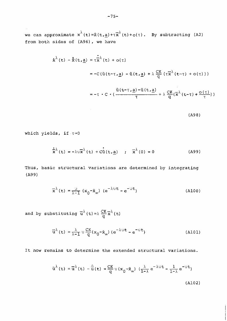
X we can approximate x (t)=8(tfa)+~xh(t)+o(r). - By subtracting (A2)

from both sides of (A96), we have

t - a - a - - CK A = -T C e ( + h -(% (t-T) + 7 o(T)))

T GI

which yields, if .T+O

Thus, basic structural variations are determined by integrating

(A9 9

CK -A and by substituting 5' (t) = A - x (t) GI

-A u (t) = _ x u--(xo-j2,) CK (e -hut - e-ut) X l GI

It now remains to determine the extended structural variations.

A -A - U x ( t ) = x (t) - x ( t ) =-(x -ftm) ( e -Au t

- u t ) A - 1 0 - e

and t o i n t e g r a t e t h e second-order d e r i v a t i v e of t h e we l fa re l o s s :

Now, t h e robus tness c o e f f i c i e n t G: has t h e form

and i s a monotonical ly decreas ing func t i on of A . I t would be

wrong, however, t o assume t h a t we should choose very l a r g e A i n

o rde r t o o b t a i n smal l va lues of 6: : very l a r g e A might r e s u l t

i n i n s t a b i l i t y of (A96) and, t h e r e f o r e , t h e ape r iod i c approxima-

t i o n xA ( t) def ined by (A99) does n o t hold any longer f o r l a r g e A .

Since t h e equat ion (A96) i s l i n e a r , i t s s t a b i l i t y i s d e t e r -

mined by i t s homogeneous p a r t :

k ( t ) =-Aux( t - r ) ; x ( t ) = O f o r t < O , x ( 0 ) = x o

To ana lyse t h e s t a b i l i t y of t h i s equat ion , we f i r s t apply Laplace

t rans fo rmat ion t o both s i d e s of it:

and r e p r e s e n t t h e r e s u l t a s a feedback system, w i t h t h e feedback

e r r o r X (s) and t h e o u t p u t v a r i a b l e Y (s) =K (s) X (s) , determined by X U - T S . t h e open-loop t r a n s f e r f u n c t i o n K ( s ) = - e . S

Now, w e can use t h e c l a s s i c a l Nyqu is t c r i t e r i o n f o r t h e

s t a b i l i t y of feedback sys tems. W e ana l yse t h e argument and t h e Xu . - jw~ module o f t h e complex v a r i a b l e K ( jw )= - , where j i s t h e jw

imaginary u n i t . W e have

The Nyquist c r i t e r i o n s t a t e s ( i n t h i s s imp le c a s e ) t h a t t h e feed-

back system i s s t a b l e i f ( ~ ( j w ) <1 f o r w o such t h a t argK( jwo) =-IT 71 . Thus , w e have w = - 0 2T O" 2 X u i < 1 gua ran tee ing s t a b i l i t y , and - = -

wo 71

which can be r e w r i t t e n a s :

However, i n c l a s s i c a l feedback systems theo ry it i s a l s o

known t h a t i f t h e Nyquis t c r i t e r i o n i s s a t i s f i e d w i t h 50% margin

( l ~ ( j w ~ ) / < 0 . 5 )

t hen t h e dynamic s o l u t i o n s i n t h e feedback system might be

reasonab ly approximated by a p e r i o d i c s o l u t i o n s ( t h e system i s

f a r enough from i t s s t a b i l i t y boundary, hence, t h e c losed- loop

s o l u t i o n might be approximated by a p e r i o d i c func t ions - - i f t h e

open-loop i t s e l f i s a p e r i o d i c ) .

There fo re , w e conclude t h a t t h e approximat ion (A99) of t h e

s o l u t i o n s o f t h e ex tended model under c losed- loop p o l i c i e s might

be reasonab ly a p p l i e d on l y i f ( A l l l ) i s s a t i s f i e d . I f w e assume 1

then w e t r ans fo rm c o n d i t i o n (A110) t o t h e form

o r , w i t h 50% margin

L which, g iven an e s t i m a t e d T and r , l i m i t s t h e maximal v and, 1 I

t h u s , t h e maximal r e l a t i v e speed o f c o n t r o l , 2 = ( 1 + 4 v ~ ) ~ - 1 r 2

2 c2 t h a t can be assumed ( say , by choosing q i n v when apply- * r q

i n g a c losed- loop p o l i c y w i t h X = X .

FOOTNOTES

1. The m o n e t a r i s t s have a l s o j u s t i f i e d t h e i r c o n s t a n t monetary growth r u l e by a rgu ing t h a t p o l i c y makers tend t o misspec i - f y t h e i r monetary r u l e s by a t t emp t i ng t o s t a b i l i z e i n t e r e s t r a t e s r a t h e r t han growth r a t e s of t h e money supp ly . The re levance of t h i s argument has become muted i n r e c e n t y e a r s a s a number o f governments-- including t h e American and t h e Br i t i sh- -have concen t ra ted i n c r e a s i n g l y on monetary s t o c k s and less on i n t e r e s t r a t e s i n t h e i r fo rmu la t ion o f monetary p o l i c i e s .

2 . I t i s f e a s i b l e t o r e l a x t h i s assumpt ion i n t h e c o n t e x t o f o u r a n a l y s i s .

3 . However, Snower (1981) has shown t h a t s y s t e m a t i c monetary p o l i c y may remain e f f e c t i v e i f t h e macro-economic model i s non l i nea r . Y e t t h e s u b j e c t o f op t ima l p o l i c y r u l e s under r a t i o n a l e x p e c t a t i o n s l i es beyond t h e scope o f t h i s paper .

4 . The extended model s e r v e s a s a gu inea p i g , an exper imenta l l a b o r a t o r y f i e l d f o r checking conc lus ions de r i ved from t h e b a s i c model. The need f o r such models i n economic a n a l y s i s is paramount and t h e r e a r e s e v e r a l a t t emp ts a t us ing such models i n po l i c y -o r i en ted a n a l y s i s . I n t h i s paper , a much more t h e o r e t i c a l l y o rgan i sed way o f us ing such models i s proposed.

Inaccuracies (a) and (b) might be formally equivalent. For example, the functional form of the Phillips curve in the extended model may be expanded by Taylor series. The co- efficients of the higher-order terms may be set to zero in the basic model. Then the mistaken parameter estimates of the basic model are responsible for its "simplistic" func- tional specification. Nevertheless, it is heuristically useful to distinguish between (a) and (b) . Thus, we denote the discrepancy above as a case of (b) rather than (a).

We make a distinction between delays and lags. A dynamic delay is the time after which the first effect of an exog- enous impulse are observed. An econometric lag is the time after which the statistically most significant effects are observed. Thus, delays are usually smaller than lags.

This combination falls in the tradition of Vanderkamp (1975) , Uornbusch and Fischer (1978) , and others.

For the discussion of other possible formulations of the decision-maker's objective function see Wierzbicki (1980a, b).

Except, possibly, at the initial time t=O, if the initial values x(O)=x and u(0)=uo do not coincide with an optimal path. In suca a case, a sharp change of m might be re- quired to bring them on an optimal path.

The case in which m lags T units of time behind u is ana- lytically uninteresting. The optimal trajectory of m(t) implied by the basic model becomes identical, in this case, with the optimal trajectory of m(t-r) of the extended model.

Here, by dual control problem we understand (following Feldbaum 1962) a problem of joint estimation of model parameters and optimization of control. Only very simple classes of dual control problems possess known solutions.

This is because the state equation, at a=a, is linear in - - x(t) and u(t). If it were not, the integrand in (53) should be based on the second derivatives of the Hamilton- ian function.

Strictly speaking, pi (t) and iii (t) are extended structural sensitivity operators, not variations; by variations we should rather understand i1 (t) (a-a) and iii (t) (a-a) . However, - - we shall use hifurther text the colloquial name variations for k1 (t) and u (t) . Clearly, ~i

'a a is semi-positive definite, as a generalized - - positive combination of semi-positive definite matrices

x i (t) xi ( t and uiT (t) ui (t) .

15. I t should be s t r e s s e d t h a t t h e methodology p r e s e n t e d i n t h i s s e c t i o n i s n o t new: i t has been developed by Wierzb ick i (1969) and g e n e r a l i z e d cons ide rab l y f o r models desc r i bed by Banach space equa t i ons by Wierzb ick i and Dontchev (1977) ; a f u l l d e s c r i p t i o n can a l s o be found i n Wierzb ick i (1977) . However, t h i s methodology has n o t , a s y e t , been a p p l i e d t o economic problems. I t goes w i t hou t say ing t h a t t h e p o s s i b l e a p p l i c a t i o n s ex tend f a r beyond t h e t h e t o p i c o f t h i s paper .

1 6 . The exp ress ion (75) i s one o f t h e s o l u t i o n s o f a q u a d r a t i c equa t ion ; t h e o t h e r s o l u t i o n (w i t h t h e s i g n be fo re t h e square r o o t i n (75) changed t o p l u s ) i s e l i m i n a t e d because

£0 on l y (75) s a t i s f i e s u fO (t) = i i ( t , a ) - a t B=0, x ( t) =8(t ,g) .

17. W e per form t h i s l i n e a r i z a t i o n by s u b t r a c t i n g h ( t , a ) = -C( i i ( t ,a ) -un - from bo th s i d e s o f ( 7 6 ) , subdiv id ing- the re-

s u l t s by B and l e t t i n g 8+0. Equ i va len t l y , w e can employ t h e theorem on t h e d i f f e r e n t i a b l e dependence o f t h e so lu - t i o n s o f d i f f e r e n t i a l equa t i ons on parameters .

18. Th is f o l l ows from t h e second Lapunov theorem on t h e s t a b i l - i t y o f n o n l i n e a r d i f f e r e n t i a l equa t i ons when a p p l i e d t o t h e

f 0 equa t i on (76) . Observe t h a t even i f 8=0, b u t x ( 0 ) #xo

( f o r example, due t o an e r r o r i n e s t i m a t i n g i n i t i a l i n f l a - t i o n a r y e x p e c t a t i o n s ) w e o b t a i n t h e u n s t a b l e v a r i a t i o n a l

'fo Q ( t , a ) 9 ( t 1 a ) - - equa t i on x (t) =C zfo (t) f o r t h e p ropaga t ion o f

v ( k , Q , a ) - f o t h e v a r i a t i o n x (0 ) o f t h e i n i t i a l s t a t e .

19. Th i s does n o t mean t h a t t h e bene f i t - t o - cos t maximizing p o l i c i e s miqht n o t be d e s i r a b l e i n o t h e r a p p l i c a t i o n s , i n

p a r t i c u l a r when e t ( t , a ) i s n e g l i g i b l e . See Wierzb ick i (1977) f o r examples OF such a p p l i c a t i o n s i n non-economic c o n t e x t .

20. Such a d i f f e r e n t i a b i l i t y has been proved by Dontchev (1980) f o r a b roader c l a s s o f problems, i n c l u d i n g t h e problem cons idered h e r e .

21. See f o o t n o t e 6 ; an e s t i m a t e of an econometr ic l a g i n u would have t o be , most probab ly , a h i ghe r number.

REFERENCES

A l c h i a n , A.A. 1970. I n f o r m a t i o n C o s t s , P r i c i n g and Resource Unemployment. I n : P h e l p s e t a l . 27-52.

A l t h a n s , M . , and P.L. F a l b . 1966. Op t ima l C o n t r o l . New York: Academic P r e s s .

B a r r o , R . J . R a t i o n a l E x p e c t a t i o n s and t h e Ro le o f Monetary P o l i c y . J a n u a r y 1976, 2 ( I ) , 1-32.

Brunner , K . and A.H. M e l t z e r , e d s . 1976. The Economics o f P r i c e and Wage C o n t r o l s . A m s t e r d a m : Nor th Ho l l and .

B u i t e r , W. Crowding Out and t h e E f f e c t i v e n e s s o f F i s c a l P o l i c y . J o u r n a l o f P u b l i c Economics. J u n e 1977, 7 ( 3 ) , 309-28.

Darby, M.R. Three and a H a l f - M i l l i o n US Employees Have Been M i s l a i d : O r , An E x p l a n a t i o n o f Unemployment, 1934-1941. J o u r n a l o f P o l i t i c a l Economy. Feb rua ry 1976, 8 4 ( 1 ) , 1-16.

D e Canio , S. R a t i o n a l E x p e c t a t i o n s and L e a r n i n g From E x p e r i e n c e . Q u a r t e r l y J o u r n a l o f Economics. F e b r u a r y 1979, 47-57.

Dontschev, A. 1980. P e r t u r b a t i o n s , Approx imat ions and S e n s i t i v - i t y A n a l y s i s o f Op t ima l C o n t r o l . A c . S c i . o f B u l g a r i a , mimeograph.

Dornbusch, R. and S. F i s c h e r . 1978. Macro-economics. N e w York: McGraw H i l l . 391-433.

Feldbaum, A.A. 1966. F o u n d a t i o n s o f t h e Theory o f Op t ima l Con- t r o l Systems. ( I n R u s s i a n ) Nauka, Moscow.

Flanagan, The US Phillips Curve and International Unemployment Rate Differentials. American Economic Review. March 1973, 63 (1) , 114-31.

Friedman, B. Optimal Expectations and the Extreme Information Assumptions of Rational Expectations Macromodels. Journal of Monetary Economies. 5 January 1979, 23-41.

Friedman, M. The Role of Monetary Policy. American Economic Review. March 1968, 58, 1-17.

Gordon, R.J. Wage-Price Controls and the Shifting Phillips Curve Curve. Brookings Papers on Economic Activity, 1972, 3(2), 385-421.

Gronau, R. Information and Frictional Unemployment. American Economic Review. June 1971, 61(3), 290-301.

Lahiri, K. Inflationary Expectations: Their Formation and Interest Rate Effects. American Economic Review. 1976, 66, 124-31.

Lawson, T. Adaptive Expectations and Uncertainty. Review of Economic Studies. January 1980, 47(2), 305-20.

Lucas, R.E. Expectations and the Neutrality of Money. Journal of Economic Theory. April 1972, 4(2), 103-24.

Lucas, R.E. Some International Evidence in Output Inflation Tradeoffs. American Economic Review. June 1973, 63(3), 326-34.

Lucas, R.E. and E.C. Prescott. Equilibrium Search and Unemploy- ment. Journal of Economic Theory. February 1974, 7(2),

Lucas, R.E. and L.A. Rapping. Price Expectations and the Phillips Curve. American Economic Review. June 1969, 59(3), 342-50.

Mackay, D.I. and R.A. Hart. Wage Inflation and the Phillips Relationship. Manchester Sch.Econ.Soc.Studies. June 1974, 42 (2) , 136-61.

Markus, L. and E.B. Lee. 1967. Foundations of Optimal Control Theory. New York: Wiley.

McCall, T.T. Economic of Information and Job Search. Quarterly Journal of Economics. February 1970, 84(1), 113-26.

McCallum, B.T. and T.K. Whitaker. The Effectiveness of Fiscal Feedback Rules and Automatic Stabilizes Under Rational Expectations. Journal of Monetary Economics, 5 April 1979, 171-86.

Mortensen, D.T. Job Search, the Duration of Unemployment and the Phillips Curve. American Economic Review. December 1970, 60 (5) , 847-61.

Park in , M . , M. Summer and R. Ward. 1976. The E f f e c t s of Excess Demand Genera l i zed Expec ta t i ons and Wage-Price Con t ro l s on I n f l a t i o n i n t h e UK: 1956-71. I n : Brunner and Me l tze r , 193-221.

Pa rk in , M. The Short-Run and Long-Run Trade-o f f s Between I n f l a - t i o n and Unemployment i n A u s t r a l i a . A u s t r a l i a n Economic Papers . December 1973, 1 2 ( 2 1 ) , 127-44.

Parsons, D.Q. Q u i e t Ra tes Over Time: A Search - In fo rmat ion Approach. American Economic Review. June 1973, 63 (3 ) , 390-401.

Phe lps , E. 1970. Money Wage Dynamics and Labor Market Equ i l i b - rium. In : Phe lps e t a l . 124-66.

--------- , ed. 1970. Microeconomic Foundat ions o f Employment and I n f l a t i o n Theory. New York: Norton.

Sa lop, S.C. Sys tema t i c Job Search and Unemployment. Review o f Economic S t u d i e s . A p r i l 1973, 40 (2) .

Sargen t , T.T. 1973. R a t i o n a l Expec ta t i ons , t h e Real Rate o f I n t e r e s t and t h e Na tu ra l Rate o f Unemployment. Brookings Papers on Economic A c t i v i t y . 2, 429-79.

--------- , A C l a s s i c a l Macroeconometric Model f o r t h e Uni ted S t a t e s . J o u r n a l o f P o l i t i c a l Economy. A p r i l 1976, 84, 207-37.

Sa rgen t , T.T. and N . Wallace. Ra t i ona l Expec ta t i ons , t h e Optimal Monetary Ins t rument and t h e Optimal Money Supply Rule. J o u r n a l o f P o l i t i c a l Economy. 1975, 83, 241-55.

--------- , Rat i ona l Expec ta t i ons and t h e Theory o f Economic P o l i c y . J o u r n a l of Monetary Economics. 2 A p r i l 1976, 169-184.

S h i l l e r , R . J . Rat i ona l Expec ta t i ons and t h e Dynamic S t r u c t u r e of Macroeconomic Models: A C r i t i c a l Review. J o u r n a l o f Monetary Economics. 4 January 1978, 1 - 4 4 .

Siven, C.H. Consumption, Supply of Labor and Search o f A c t i v i t y i n an In tempora l P e r s p e c t i v e . Swedish J o u r n a l o f Economics. March 1974, 7 (1) , 44-61.

Snower, D . J . 1981. Ra t i ona l Expec ta t i ons , N o n l i n e a r i t i e s and t h e E f f e c t i v e n e s s o f Monetary Po l i cy . Mimeograph.

Tay lo r , J . B . Monetary P o l i c y During a T r a n s i t i o n t o R a t i o n a l Ex- p e c t a t i o n s . J o u r n a l o f P o l i t i c a l Economy. October 1975, 83, 1009-21.

Tobin, J. and W. Buiter. Fiscal and Monetary Policies, Capital Formation and Economic Activity. Forthcoming in G.v. Furst- enberg: The Government and Capital Formation.

Turnovsky, S.J. The Expectations Hypothesis and the Aggregate Wage Equation: Some Empirical Evidence for Canada. Economica. February 1972, 39 (153) , 1-17.

----- , Empirical Evidence of the Formation of Price Expectations. Journal of the American Statistical Association. 1970, 65, 1441-54.

Vanderkamp, J. Wage Adjustment, Productivity and Price Change Expectations. Review of Economic Studies. January 1972, 39 (1) , 61-72.

Vanderkamp, J. Inflation: A Simple Friedman Theory with a Phillips Twist. Journal of Monetary Economics. 1975, 117-122.

Wierzbicki, A.P. 1969. Unified Approach to the Sensitivity Analysis of Optimal Control Systems. IVth Congress of IFAC, Warsaw.

Wierzbicki, A.P. Maximum Principle for Processes with Multiple Control Delays. (In Russian) Automatics and Remote Control. October 1970, 13-20.

Wierzbicki, A.P. and A.L. Dontchev. Basic Relations in Perfor- mance Sensitivity Analysis of Optimal Control Systems. Control and Cybernetics. 1974, 3, 119-139.

Wierzbicki, A.P. 1977. Models and Sensitivity of Control Systems. (In Polish) WNT, Warsaw.

Wierzbicki, A.P. 1980a. A Mathematical Basis for Satisfying Decision-Making. International Institute for Applied Systems Analysis, Laxenburg, Austria: WP-80-90.

Wierzbicki, A.P. 1980b. 14ultiobjective Trajectory Optimization and blodel Semiregularization. International Institute for Applied Systems Analysis, Laxenburg, Austria: UP-80-181.