Immigration, Worker-Firm Matching, and

Inequality

Jaerim Choi* Jihyun Park**

University of Hawaii at Manoa KISDI

August 2, 2018

Abstract

This paper develops a novel framework of worker-firm matching to study the dis-

tributional impacts of low-skilled immigration on native workers. Adopting an as-

signment model from the trade literature, we build a theoretical model where the

inflow of immigrants affects natives through the change in worker-firm matching.

Theory predicts that the inflow of low-skilled immigrants pushes natives up to match

with more productive firms. With complementarity assumption, the benefits are bi-

ased toward skilled workers, and inequality rises among native workers. Using Cen-

sus and IPUMS American Community Survey over the period 1980-2010, we provide

empirical evidence that immigration raises inequality through the matching channel.

Keywords: Immigration; Matching; Inequality.

JEL Code: F22, F66, J31.

*Department of Economics, University of Hawaii at Manoa, choijm@hawaii.edu**Korea Information Society Development Institute, jhnpark@kisdi.re.kr

1 Introduction

What are the distributional effects of immigration in the U.S.? This paper proposes a

new framework, a matching between workers and firms, to think about the impacts of

immigration on inequality.

Immigrants in the U.S. labor market are characterized by less educated immigrants

- there are relatively more immigrants at the lower end of the skill distribution. Thus,

the influx of immigrants may differently affect natives with heterogeneous skills, which

leads to a change in inequality in the U.S. Therefore, it is essential to incorporate hetero-

geneous skills into the theoretical immigration model, not based on representative agent

models, to analyze the impact of immigration on inequality in the U.S. In addition to

heterogeneity in the inflows of immigrants, the U.S. labor market is characterized by pos-

itive assortative matching (PAM) between workers and firms: High-skilled workers are

matched with high-productive firms. Moreover, log wage schedules are increasing and

convex in education levels (Lemieux, 2006, 2008).

Based on these observations in the U.S. labor market, we build a theoretical immigra-

tion model of matching between heterogeneous workers and heterogeneous firms with

complementary production technology in the framework of monopolistic competition

(Sampson, 2014). Heterogenous firms are paired up with heterogeneous workers to pro-

duce differentiated goods. In equilibrium, our model replicates the positive assortative

matching and the convex log wage schedule which are observed in the U.S. labor mar-

ket. When immigrants arrive in the destination country, it changes the skill distribution

of workers, and the influx changes the matching mechanism between workers and firms.

Because the wages are determined by both the skill level of workers and the productivity

level of firms, there would be distributional consequences after immigration.

We analyze two hypothetical cases of immigration. First, we assume that the skill

distribution of immigrants is identical to that of natives. In this case, the matching mech-

anism and the wage function do not change from immigration. Second, we consider a

1

case where immigrants are relatively less skilled than natives. The case of low-skilled

immigration is of great importance because the low-skilled immigration characterizes the

U.S. immigration. The distributional implication, in the second case, presents a starking

contrast to the first case. The model predicts that immigrant inflow changes the matching

mechanism between workers and firms. Native workers can now be paired up with firms

with higher productivities, which increases inequality. Due to the complementary pro-

duction technology between worker’s skill and firm’s productivity, more skilled workers

benefit more from the re-matching process.

We empirically test whether the theory applies to the U.S. local labor markets during

the period from 1980 to 2010. We use U.S. Census 1980, 1990, 2000 and IPUMS Ameri-

can Community Survey 2008-2012 and exploit the variation in the share of immigrants

across commuting zone-year. We assume that immigrants tend to be less-skilled than na-

tives since the foreign-born percentage of the U.S. population in a less educated group is

overrepresented than in other groups (Peri, 2016) and the absolute number of immigrants

in this group outweighs the number of other groups. We use a Baltik-type shift-share

instrument to deal with potential endogeneity issues.

Using the two-stage least squares estimation technique, we demonstrate that the in-

flux of low-skilled immigrants increases inequality within natives. We further explore

whether the increase in inequality comes from the worker-firm matching channel. Be-

cause we cannot directly observe worker-firm matching in our dataset, we define each

commuting zone - industry pair as a proxy unit for a firm. Using a variant of Mincerian

wage regression, we decompose worker’s wage into components related to observable

worker characteristics, unobservable firm heterogeneity (commuting zone - industry het-

erogeneity), other unobservable fixed effects, and residual variation. We use the estimated

firm heterogeneity as a proxy for time-invariant productivities of native workers’ match-

ing counterparts. Empirical results show that low-skilled immigration induces native

workers to match with more productive firms.

2

2 Related Literature

There has been extensive literature on the effect of immigrants on the wages of natives

(Borjas, 2003; Card, 2009; Ottaviano and Peri, 2012; Basso and Peri, 2015). However, stud-

ies in this research arena have not come to a single conclusion as to the direction of the

impact of immigration on the wages of native workers. Borjas (2003) argues that immi-

gration adversely affects the wages of competing native workers. The author assumes

that workers with the same education and different work experience in a national mar-

ket are not perfect substitutes and uses the variations in schooling-experience groups to

measure the wage impact of immigration. On the contrary, Ottaviano and Peri (2012) find

a small positive effect on native wages. Using the national approach as in Borjas (2003),

this study estimates the elasticity of substitution across a different group of workers and

uses the estimated elasticities to calculate the total wage effect of immigration. They find a

small but significant degree of imperfect substitutability between natives and immigrants

under the same education-experience cell, which leads to the overall positive wage effect

of immigration. Similar to Ottaviano and Peri (2012), Basso and Peri (2015) find a zero to

a positive impact of immigration on the wages of native workers using the 2SLS method

with a shift-share instrument. Card (2009) explores the impact of immigration on wage

inequality using cross-city variations in the U.S. The author finds that immigration had

a small effect on wage inequality among natives. However, considering immigrants are

counted in total population, the effect of immigration on total wage inequality becomes

positive as immigrants tend to locate in the upper and lower tails of the skill distribution.

We contribute to this literature by building a new immigration framework to analyze the

impact of immigration on the wages and inequality of native workers. The modeling

framework is based on the heterogeneous workers and heterogeneous firms which allow

us to analyze diverse aspects of immigration on natives. The prediction from the model

and empirical results shed some light on the impact of immigration on the wages of native

workers.

3

Researchers have also studied more micro-founded mechanisms for the impact of

immigration on the wages of native-born workers. Peri and Sparber (2009) argue that

native-born workers and foreign-born workers specialize in different production tasks so

that large influx of less-educated immigrants may not necessarily substitute less-educated

native workers. In the model, immigration will re-allocate task supply in which foreign-

born workers specialize in manual tasks while native workers specialize in communica-

tion tasks. The task specialization mechanism attenuates the negative wage impact of

immigration on native workers. Hunt and Gauthier-Loiselle (2010) find evidence of the

positive spillovers of skilled migration on boosting innovation in the U.S. As immigrants

are more concentrated in science and engineering occupations than natives in those oc-

cupations, immigrants increase innovation as measured by US patents per capital. Since

scientific and engineering knowledge transfers occur easily, this positive spillover makes

native workers better off. Ortega and Peri (2014) show that openness to immigration leads

to higher income per capita. This positive effect operates through an increased total factor

productivity from increased diversity and ideas in the host country. We introduce a new

mechanism, “worker-firm matching,” to explain the distributional effects of immigrants

on the natives. As immigration can be seen as matching between immigrant workers

and native firms, we incorporate the standard matching framework into the model and

analyze how different types of immigration affect the matching function, which maps

workers’ skills to firms’ productivities, in the host country. Through the change in the

skill distribution of workers from immigration, native workers are paired up with new

firms with higher productivities. This matching mechanism affects the wages of native

workers, thereby changing inequality among native workers.

Our insight on immigration, defined as matching between immigrants and native

firms, is based upon the concept of globalization in Kremer and Maskin (1996, 2006).

Kremer and Maskin (1996) propose a model of production by workers of different skills

with complementarity between two tasks. In a closed economy setting, they argue that

4

segregation of high-skilled and low-skilled workers into separate firms will lead to wage

inequality. Kremer and Maskin (2006) extend the analysis to a two-country framework

and analyze the impact of globalization, which is defined as workers from different coun-

tries being able to form a team in the same firm. Globalization enables high-skilled work-

ers in poor countries to be matched with more skilled workers in rich countries. Low

skilled workers in the poor countries are marginalized due to globalization because their

skill levels are so low that rich country workers do not want to match with them.

Our theoretical framework is also closely related to the burgeoning literature in in-

ternational trade that uses an assignment model with heterogeneous workers (Antras,

Garicano and Rossi-Hansberg, 2006; Ohnsorge and Trefler, 2007; Costinot and Vogel,

2010; Sampson, 2014; Grossman, Helpman and Kircher, 2017; Grossman and Helpman,

2018). Antras, Garicano and Rossi-Hansberg (2006) propose a knowledge-based hier-

archy model to analyze the impact of cross-country team formation on the structure of

wages. Ohnsorge and Trefler (2007) study the implication of two-dimensional worker het-

erogeneity and worker sorting on international trade. Costinot and Vogel (2010) develop

tools and techniques to analyze the factor allocation and factor prices in a Roy-like assign-

ment model with a continuum of workers and a continuum of tasks. Grossman, Helpman

and Kircher (2017) develop two industries and two heterogeneous factors of production

framework in which they study the distributional effects of international trade.

In this paper, we base our model upon Sampson (2014)’s monopolistic competition as-

signment model. Then, we apply the monotone comparative statics technique in Costinot

and Vogel (2010) to derive analytical results about the distributional impacts of immigra-

tion. Immigration changes the skill distribution of workers, thus changes the matching

mechanism in the model. The theoretical model developed in this paper, to the best of our

knowledge, is the first application of the assignment model with heterogeneous workers

in the immigration literature.

5

3 Some Observations in the U.S. Labor Market

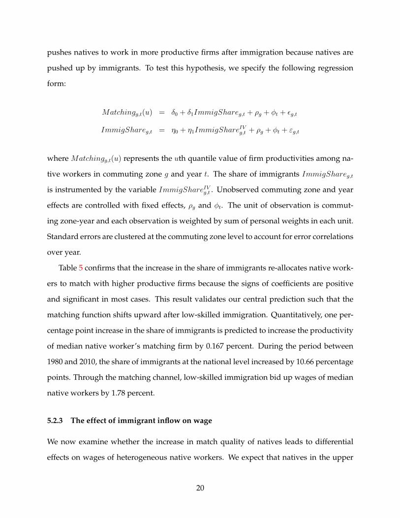
Fact I. Natives and immigrants are heterogeneous in skills.

There are relatively more immigrants at the lower end of the education distribution,

i.e., immigrant workers have lower education levels compared to native workers (See

Figure 1). Native workers are concentrated in high school graduates, but a significant

share of immigrant workers report their education as none. Moreover, immigrants are

less likely to have excellent communication skills, such as language, than comparably-

educated, native-born workers (Peri and Sparber, 2009). Thus, the influx of immigrants

into the U.S. labor market can be characterized as an increase in the supply of workers

with low skills.

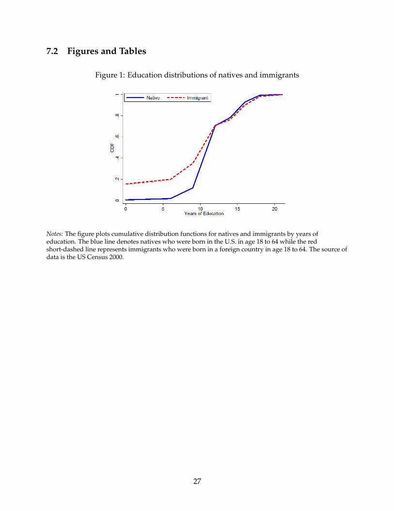
Fact II. Worker-Firm matching shows positive assortative matching.

We use U.S. census data to approximate firms by commuting zone-industry pairs. Be-

cause firm productivities are unobservable to researchers, we set up a variant of Mince-

rian type regression and compute time-invariant commuting zone-industry fixed effects

to proxy for firm productivities (See Section 5.1.5 for more details). Within each firm,

we calculate average schooling years and average imputed log hourly wages of workers.

In the top panel of Figure 2, more educated workers are paired up with more produc-

tive firms. In the bottom panel of Figure 2, higher paid workers are matched with more

productive firms. There is a positive association between worker skills and firm pro-

ductivities. In this literature, we use positive assortative matching (PAM) to denote this

relationship. This relationship also holds for other years (1980, 1990, and 2010).

Fact III. Log wage function is strictly increasing and convex in skills.

Lemieux (2006, 2008) argues that log wages have become an increasingly convex func-

tion of years of education. In 1973 - 1975, the log wage appeared to be a linear function in

years of education. However, in 2003 - 2005, this log wage function had become a convex

6

function in that the return to post-secondary education is much higher than the return to

elementary and secondary education. We revisit this finding using US Census dataset.

First, we show that log hourly wage is strictly increasing in years of education in each

year and returns to an additional year of education is much higher for those with high

school education or more compared to those with secondary education or less. Moreover,

the log wage gap within the same education level between the year 1980 and the year

2010 increases in years of education (See Figure 3).

4 The Model

We build a theoretical immigration framework that can replicate these three observa-

tions in the U.S. labor market: 1. Heterogeneity in skills between immigrants and na-

tives, 2. Positive assortative matching between workers and firms, and 3. Log wage

function is increasing and convex in education levels. More specifically, our model is

based upon Sampson (2014)’s matching model in which heterogeneous firms hire hetero-

geneous workers to produce differentiated goods in a monopolistic competition frame-

work. Using this framework, we extend the model to allow for immigration and study

the distributional effects of different cases of immigration.

4.1 Environment

Consider an economy populated by a mass N of workers indexed by skill level z, and a

mass M of firms indexed by productivity level ϕ. The cumulative distribution of skills is

given by H(z), which is twice differentiable and has a positive density H ′(z) > 0 on the

bounded support [zmin, zmax] with zmin > 0. Similarly, the cumulative distribution of firm

productivities is given by G(ϕ), which is twice differentiable and has a positive density

G′(ϕ) > 0 on the bounded support [ϕmin, ϕmax] with ϕmin > 0. Firms with different

productivities hire different types of workers to produce differentiated goods, indexed

7

by ω, using worker as the sole input to production.

The preference of each individual is given by a CES utility over a continuum of differ-

entiated goods:

U =

[∫ω∈Ω

x(ω)σ−1σ dω

] σσ−1

where Ω is the set of available goods and σ > 1 is the elasticity of substitution between

goods. It follows that the demand for any variety ω is given by:

x(ω) = XP σp(ω)−σ

where X is the aggregate output of composite good, P :=[∫ω∈Ω

p(ω)1−σdω] 1

1−σ is the

aggregate price, and p(ω) is the price of differentiated good ω. Without loss of generality,

we normalize the aggregate price P equal to one. Then, the demand for variety ω can be

expressed as:

x(ω) = Xp(ω)−σ.

Consider a firm that produces variety ω using productivity ϕ and that hires a set Lω of

workers with densities lw(z). Then, the output is given by:

x(ω) =

∫z∈Lω

ψ(ϕ, z)lw(z)dz.

Assumption 1. The productivity function ψ(ϕ, z) is twice continuously differentiable, strictly

increasing, and strictly log supermodular.

Assumption 2. The log productivity function lnψ(ϕ, z) is twice continuously differentiable,

strictly increasing, and second partial derivatives with respect to z are strictly positive.

8

4.2 Profit Maximization

Each firm chooses the employment size and the worker skill level to maximize the fol-

lowing profit:

π(l, z;ϕ) = X1σ [ψ(ϕ, z)l]

σ−1σ − w(z)l,

where w(z) is the wage paid to workers of skill level z. The first order conditions of the

profit maximization problem can be written as follows:

∂π

∂z=σ − 1

σX

1σ [ψ(ϕ, z)l]−

1σ ψz(ϕ, z)− w′(z) = 0,

∂π

∂l=σ − 1

σX

1σ [ψ(ϕ, z)l]−

1σ ψ(ϕ, z)− w(z) = 0.

Rearranging the two conditions, we can obtain the differential equation that characterizes

the trade off relation between the productivity and the wage as follows:

ψz(ϕ, z)

ψ(ϕ, z)=w′(z)

w(z). (1)

Assumption 1 and equation (1) dictate the equilibrium matching pattern, which is the

positive assortative matching (PAM) between firm types and worker types. Denote m(z)

as a matching function that maps worker skill to firm productivity, and w(z) as an equi-

librium wage function.

Assumption 2 dictates the equilibrium log wage schedule. From equations (1), we

know that the partial derivatives of log productivities with respect to skill z are identi-

cal to partial deriviatives of log wage function with respect to skill z. Because the log

productivities are strictly increasing and convex in skill z from Assumption 2, log wage

schedule lnw(z) is strictly increasing and convex in skill z. The equilibrium matching

function and wage function replicate the patterns in the U.S. labor market: the positive

assortative matching between workers and firms (Fact II) and the log wage schedule is

9

strictly increasing and convex in years of eduaction (Fact III).

Using the profit maximization condition, the optimal number of workers, the price,

and the profit that a firm with productivity ϕ, are given by,

l(z;ϕ) =

(σ − 1

σ

)σXψ (ϕ, z)σ−1w(z)−σ,

p(ϕ) =σ

σ − 1

w(z)

ψ(ϕ, z),

π(ϕ) = σ−σ(σ − 1)σ−1X

(w(z)

ψ(ϕ, z)

)1−σ

.

4.3 Labor Market Clearing

Consider a set of workers [zmin, z] and the set of firms [ϕmin,m(z)] that matched with these

workers in the equilibrium. The labor market clearing condition can be expressed as:

M

∫ m(z)

ϕmin

(σ − 1

σ

)σXψ

(ϕ,m−1(ϕ)

)σ−1w(m−1(ϕ))−σdG(ϕ) = N

∫ z

zmin

dH(z)

where the left-hand side is the demand for workers by firms with productivity level be-

tween ϕmin andm(z) and the right-hand side is the supply of workers matched with those

firms. Differentiating this equation with respect to z yields,

m′(z) =N

MX

(σ

σ − 1

)σw(z)σ

ψ(m(z), z)σ−1

H ′(z)

G′(m(z)), for all z ∈ [zmin, zmax] (2)

with the two boundary conditions ϕmax = m(zmax) and ϕmin = m(zmin). This differential

equation with two boundary conditions, together with equation (1), uniquely determine

the matching function m(z) and the wage function w(z) .

10

4.4 Equilibrium

Definition 1. The equilibrium is characterized by a set of functions,m(z) (the matching function)

and w(z) (the wage function), such that

(i) Optimality: Firms maximize profits that satisfy equation (1),

(ii) Labor Market Clearing: The labor markets clear as in equation (2)

4.5 The Distributional Effects of Immigration

Suppose that this economy, entirely composed of natives, starts to open doors to immi-

grants. Because immigrants have lower education levels and communication skills com-

pared to natives (See Fact I), we consider a case where low-skilled immigrant workers

migrate to the destination country. We assume that they are integrated into the pool of

workers and that they are relatively less-skilled than native workers. We can model this

case as follows. First, the number of workers increases such that N ′ > N where N ′ de-

notes the number of workers after immigration, and N represents the number of workers

before immigration. Second, the skill distribution of workers after immigration changes

such thath′(z′)

h′(z)≤ h(z′)

h(z)for all z′ ≥ z where h′(z) is the skill distribution function after

immigration and h(z) denotes the skill distribution function before immigration. We can

decompose the effect of immigration into two channels: 1) the change in the number of

workers and 2) the change in the worker skill distribution.

Proposition 1. Suppose that the number of workers increases such that N ′ > N . Then,

(i) The matching function, m(z), does not change;

(ii) The wage function, w(z), does not change.

Proof. See Appendix 7.1.1.

In this case, the increase in the size of the workers does not affect matching patterns

and wages. The impact of immigration on native workers is neutral. However, based on

the Fact I, we analyze the impact of the change in the worker skill distribution as follows.

11

Proposition 2. Suppose that there are relatively more low-skilled workers after immigration such

thath′(z′)

h′(z)≤ h(z′)

h(z)for all z′ ≥ z. Then,

(i) The matching function, m(z), shifts upward;

(ii) The wage inequality rises such thatw′(z′)

w′(z)≥ w(z′)

w(z)for all z′ ≥ z.

Proof. See Appendix 7.1.2.

Since immigrant workers are less-skilled than native workers, the lower part of the

worker’s skill distribution thickens, which induces native workers to match with more

productive firms: the upward shift of the matching functionm(z). Due to the log-supermodularity

of the production function, more skilled workers benefit more from the increase in match

quality than less skilled workers. Therefore, the wage inequality rises.

4.6 Extension

We extend the impacts of immigration to a case in which the skill distribution of immi-

grants is more diverse than that of natives.

Proposition 3. Suppose that there are more diverse workers after immigration such thath′(z′)

h′(z)≥

h(z′)

h(z)for all z′ ≥ z ≥ z and

h′(z′)

h′(z)≤ h(z′)

h(z)for all z > z′ ≥ z. Then,

(i) There exists a skill level z∗ such thatm′(z) ≥ m(z) for all z ∈ [zmin, z∗], andm′(z) ≤ m(z)

for all z ∈ [z∗, zmax];

(ii) The wage inequality increases among low-skilled workers such thatw′(z′)

w′(z)≥ w(z′)

w(z)for

all z∗ > z′ ≥ z > zmin and the wage inequality reduces among high-skilled workers such thatw′(z′)

w′(z)≤ w(z′)

w(z)for all zmax > z′ ≥ z > z∗.

Proof. See Appendix 7.1.3.

Because immigrant workers are concentrated in the extreme tails of the skill distri-

bution, the impacts of immigration differ across groups. Among high-skilled natives,

12

immigration causes native workers to match with less productive firms. However, im-

migration induces native workers to be paired up with more productive firms among

low-skilled native workers. The combined effects lead to the increase in wage inequality

among the low-skilled group and the decrease in wage inequality among the high-skilled

group. Hence, the mid-skilled native workers relatively benefit the most from the case of

immigration with diverse immigrants.

5 Empirical Analysis

In this section, we analyze whether our theoretical model can explain the effect of the

influx of immigrants in the U.S. from 1980 through 2010. First, we give an overview of

our dataset and construct key variables. Then we empirically show that the immigrant

inflow increases the inequality in the U.S., consistent with our theory, and show that the

worker-firm matching channel operates.

5.1 Data and Variables

5.1.1 Data overview

Our primary datasets are 5% 1980, 1990, 2000 U.S. Census and 2009-2011 3-year IPUMS

American Community Survey for 2010. We restrict samples to all individuals in age 18

to 64. ‘Immigrants’ refer to individuals who were born in a foreign country, and ‘natives’

refer to those who were born in the U.S.1 We use commuting zones as geographical units

following Autor, Dorn and Hanson (2013) and Basso and Peri (2015). An instrumental

variable for the share of immigrants in each year and commuting zone is estimated by

a shift-share method based on the foreign-born population in the 1% 1950 U.S. Census.

Hourly wages are calculated by dividing the wage and salary income by weeks worked

1U.S. territories are excluded.

13

and usual hours worked per week. Hourly wages in the lowest and the highest 1% of the

distribution and those of less than one dollar are dropped.

Table 1 presents descriptive statistics for natives and immigrants. The share of im-

migrants at the national level in our sample gradually rises from 6.45% in 1980, 9.37% in

1990, 13.83% in 2000, to 17.11% in 2010. It also shows that immigrants tend to have a lower

share of female and lower share of managers. The share of female and the share of man-

ager in 2010 are 43.44% and 6.62% among immigrants, respectively, while they are 49.31%

and 9.04% among natives. The level of education shows that immigrants are less-skilled

than natives. In 2010, 6.30% of natives had less than high school while 26.08% of immi-

grants have less than high school. In the same year, 39.38% of natives have more than a

high school degree while 35.45% of immigrants have more than a high school degree.

5.1.2 Commuting zone

We use commuting zones as primary geographical units following Autor, Dorn and Han-

son (2013) and Basso and Peri (2015). States are too large to represent local labor markets,

and counties are too small and often do not overlap with labor market regions. Metropoli-

tan areas include regions around urban areas and have a limitation in representing rural

areas. Commuting Zones are developed by Tolbert and Sizer (1996) to approximate lo-

cal labor markets, and they can be consistently constructed over the full period of our

analysis.

The U.S. Census and American Community Survey files provide geographical units

that are smaller than states – State Economic Areas (1950), Country Groups (1980), and

Public Use Micro Area (PUMA, 1990, 2000, 2009-2011). These geographical units are

mapped to commuting zones using the mapping file (http://ddorn.net/). While many

units fall into a single CZ, some geographical units are matched to several CZs with each

probability. For example, 20% of workers in a PUMA commute to the first CZ and 80% to

the second CZ. Each observation in that PUMA is now split into two CZs with probability

14

.2 and .8, and personal weights are also split by .2 and .8 (Autor, Dorn and Hanson, 2013).

5.1.3 Share of immigrants

The number of immigrants in each commuting zone is endogenously determined by the

pull factors of each region, such as labor market conditions. To remove the endogeneity,

we construct an instrumental variable for the share of immigrants in each commuting

zone and year (ImmigShareg,t) by a shift-share method based on the foreign-born popu-

lation in 1950 US Census as follows:

P opg,o,t = Popg,o,1950 ∗PopUS,o,tPopUS,o,1950

(o = US and other origin countries)

ImmigShareIVg,t =

∑o 6=US P opg,o,t∑o P opg,o,t

(3)

where g denotes a commuting zone, o represents a origin country, and t is year. We group

origin countries into 16 origin regions.2 For each origin region o, immigrant population in

1950 in commuting zone g (Popg,o,1950) is increased by the national increase rate between

1950 and year t ( PopUS,o,tPopUS,o,1950

).

The stock of the native population in each commuting zone and year is estimated sim-

ilarly and noted as o = US. We calculate the stock of all immigrants in each commuting

zone and year by aggregating the number of immigrants over all origin regions, excluding

the U.S. Lastly, the share of immigrants in commuting zone g and year t, ImmigShareIVg,t ,

is calculated by the stock of all immigrants (∑

o 6=US P opg,o,t) divided by the sum of both

immigrants and natives (∑

o P opg,o,t).

We then examine the weak instrumental variables problem. The first stage regression

result shows that the F statistics is 70.32 which is higher than 16.38 – 10% critical value

2Sixteen origin regions are United States, Other North America, Central America and Caribbean,South America, Northern Europe, United Kingdom and Ireland, Western Europe, Southern Europe, Cen-tral/Eastern Europe, Russian Empire, East Asia, Southeast Asia, India/Southwest Asia, Middle East/AsiaMinor, Africa, and Oceania.

15

for one endogenous variable and one excluded instrument. Hence, we reject the null

hypothesis that our shift-share instrument is weak.

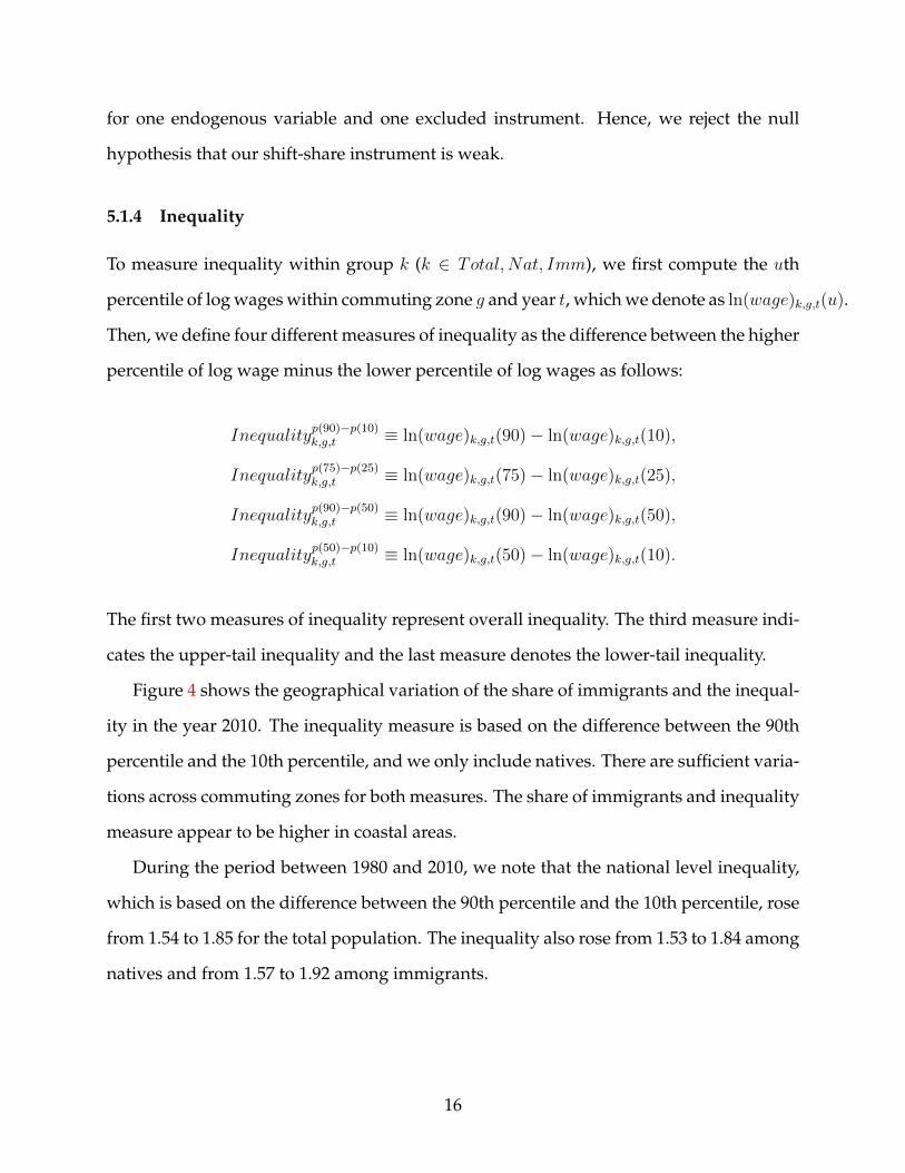
5.1.4 Inequality

To measure inequality within group k (k ∈ Total, Nat, Imm), we first compute the uth

percentile of log wages within commuting zone g and year t, which we denote as ln(wage)k,g,t(u).

Then, we define four different measures of inequality as the difference between the higher

percentile of log wage minus the lower percentile of log wages as follows:

Inequalityp(90)−p(10)k,g,t ≡ ln(wage)k,g,t(90)− ln(wage)k,g,t(10),

Inequalityp(75)−p(25)k,g,t ≡ ln(wage)k,g,t(75)− ln(wage)k,g,t(25),

Inequalityp(90)−p(50)k,g,t ≡ ln(wage)k,g,t(90)− ln(wage)k,g,t(50),

Inequalityp(50)−p(10)k,g,t ≡ ln(wage)k,g,t(50)− ln(wage)k,g,t(10).

The first two measures of inequality represent overall inequality. The third measure indi-

cates the upper-tail inequality and the last measure denotes the lower-tail inequality.

Figure 4 shows the geographical variation of the share of immigrants and the inequal-

ity in the year 2010. The inequality measure is based on the difference between the 90th

percentile and the 10th percentile, and we only include natives. There are sufficient varia-

tions across commuting zones for both measures. The share of immigrants and inequality

measure appear to be higher in coastal areas.

During the period between 1980 and 2010, we note that the national level inequality,

which is based on the difference between the 90th percentile and the 10th percentile, rose

from 1.54 to 1.85 for the total population. The inequality also rose from 1.53 to 1.84 among

natives and from 1.57 to 1.92 among immigrants.

16

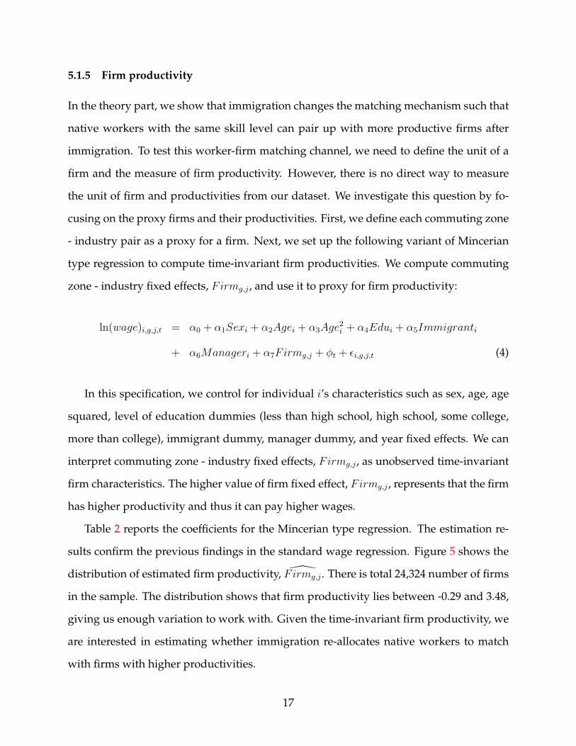
5.1.5 Firm productivity

In the theory part, we show that immigration changes the matching mechanism such that

native workers with the same skill level can pair up with more productive firms after

immigration. To test this worker-firm matching channel, we need to define the unit of a

firm and the measure of firm productivity. However, there is no direct way to measure

the unit of firm and productivities from our dataset. We investigate this question by fo-

cusing on the proxy firms and their productivities. First, we define each commuting zone

- industry pair as a proxy for a firm. Next, we set up the following variant of Mincerian

type regression to compute time-invariant firm productivities. We compute commuting

zone - industry fixed effects, Firmg,j , and use it to proxy for firm productivity:

ln(wage)i,g,j,t = α0 + α1Sexi + α2Agei + α3Age2i + α4Edui + α5Immigranti

+ α6Manageri + α7Firmg,j + φt + εi,g,j,t (4)

In this specification, we control for individual i’s characteristics such as sex, age, age

squared, level of education dummies (less than high school, high school, some college,

more than college), immigrant dummy, manager dummy, and year fixed effects. We can

interpret commuting zone - industry fixed effects, Firmg,j , as unobserved time-invariant

firm characteristics. The higher value of firm fixed effect, Firmg,j , represents that the firm

has higher productivity and thus it can pay higher wages.

Table 2 reports the coefficients for the Mincerian type regression. The estimation re-

sults confirm the previous findings in the standard wage regression. Figure 5 shows the

distribution of estimated firm productivity, F irmg,j . There is total 24,324 number of firms

in the sample. The distribution shows that firm productivity lies between -0.29 and 3.48,

giving us enough variation to work with. Given the time-invariant firm productivity, we

are interested in estimating whether immigration re-allocates native workers to match

with firms with higher productivities.

17

5.2 Empirical Results

In the theoretical model, we predict that the inflow of immigrants increases the inequality

within natives. A significant share of immigrants are low-skilled immigrants, and low-

skilled immigrants tend to be even lower skilled than low-skilled natives. Thus, under the

positive assortative matching, we predict that natives would be pushed up to be matched

to more productive firms when immigrants arrive at the destination country. Due to

the log supermodularity, better workers benefit more from the increase in the quality

of matched firms and thus the inequality within natives increases. In this section, we

empirically analyze the impact of immigrants in the U.S. from 1980 to 2010.

5.2.1 The effect of immigrant inflow on inequality

First, we test whether the inflow of immigrants increases the inequality in the U.S. We fit

models of the following form:

Inequalityg,t = β0 + β1ImmigShareg,t + ρg + φt + εg,t

ImmigShareg,t = γ0 + γ1ImmigShareIVg,t + ρg + φt + εg,t

where Inequalityg,t represents the inequality in commuting zone g and year t. The share of

immigrants ImmigShareg,t is instrumented by the variable ImmigShareIVg,t . Unobserved

commuting zone and year effects are controlled with fixed effects, ρg and φt. The unit

of observation is commuting zone-year and each observation is weighted by sum of per-

sonal weights in each unit. Standard errors are clustered at the commuting zone level to

account for error correlations over year.

The first two columns of Table 3 estimate the model using all individuals, including

both natives and immigrants. The coefficient of 0.754 in column 1 indicates that one per-

centage point increase in the share of immigration is predicted to increase the relative

wage gap between the 90th percentile and the 10th percentile by 0.75 percent. Column 2

18

shows that one percentage point increase in the share of immigration is associated with

an increase in the relative wage gap between the 75th percentile and the 25th percentile

by 0.79 percent. In columns 3 and 4 of Table 3, we confine our analysis to natives. The

coefficients of 0.921 and 0.796 are higher than the case of all individuals, which provides

substantial evidence that immigration affects native workers. Columns 5 and 6 of Table 3

provide the results of the case of immigrants. The coefficients of 0.498 and 0.545 are lower

than the case of natives, which indicates that the distributional impact of immigration is

stronger for natives.

In Table 4, we repeat the two-stage least squares regression analysis using different

measures of inequality. We define the upper-tail inequality, p(90) - p(50), as the log wage

difference between the 90th percentile and the 50th percentile. We also define the lower-

tail inequality, p(50) - p(10), as the log wage difference between the 50th percentile and

the 10th percentile. In columns 3 and 4 of Table 4 focusing on natives, both the upper-

tail inequality and the lower-tail inequality increase from immigration, and the impact

is stronger for the lower-tail inequality. This is different from total (column 1 and 2) or

immigrant (column 5 and 6) population where the increase in inequality is mostly in the

upper-tail, suggesting that inflow of low-skilled immigrants affects low-skilled natives

more than the high-skilled natives.

5.2.2 The effect of immigrant inflow on matching

Using the estimated firm productivities, we can assign values to each native worker as

follows:

Matchingi,g,j,t ≡ F irmg,j

where Matchingi,g,j,t refers to a firm productivity level that native worker i who works at

the firm (g, j) in year t. In each commuting zone - year, we further compute the uth quan-

tile value of firm productivities among native workers and denote this as Matchingg,t(u).

We expect that low-skilled immigration shifts the matching function upward, which

19

pushes natives to work in more productive firms after immigration because natives are

pushed up by immigrants. To test this hypothesis, we specify the following regression

form:

Matchingg,t(u) = δ0 + δ1ImmigShareg,t + ρg + φt + εg,t

ImmigShareg,t = η0 + η1ImmigShareIVg,t + ρg + φt + εg,t

where Matchingg,t(u) represents the uth quantile value of firm productivities among na-

tive workers in commuting zone g and year t. The share of immigrants ImmigShareg,t

is instrumented by the variable ImmigShareIVg,t . Unobserved commuting zone and year

effects are controlled with fixed effects, ρg and φt. The unit of observation is commut-

ing zone-year and each observation is weighted by sum of personal weights in each unit.

Standard errors are clustered at the commuting zone level to account for error correlations

over year.

Table 5 confirms that the increase in the share of immigrants re-allocates native work-

ers to match with higher productive firms because the signs of coefficients are positive

and significant in most cases. This result validates our central prediction such that the

matching function shifts upward after low-skilled immigration. Quantitatively, one per-

centage point increase in the share of immigrants is predicted to increase the productivity

of median native worker’s matching firm by 0.167 percent. During the period between

1980 and 2010, the share of immigrants at the national level increased by 10.66 percentage

points. Through the matching channel, low-skilled immigration bid up wages of median

native workers by 1.78 percent.

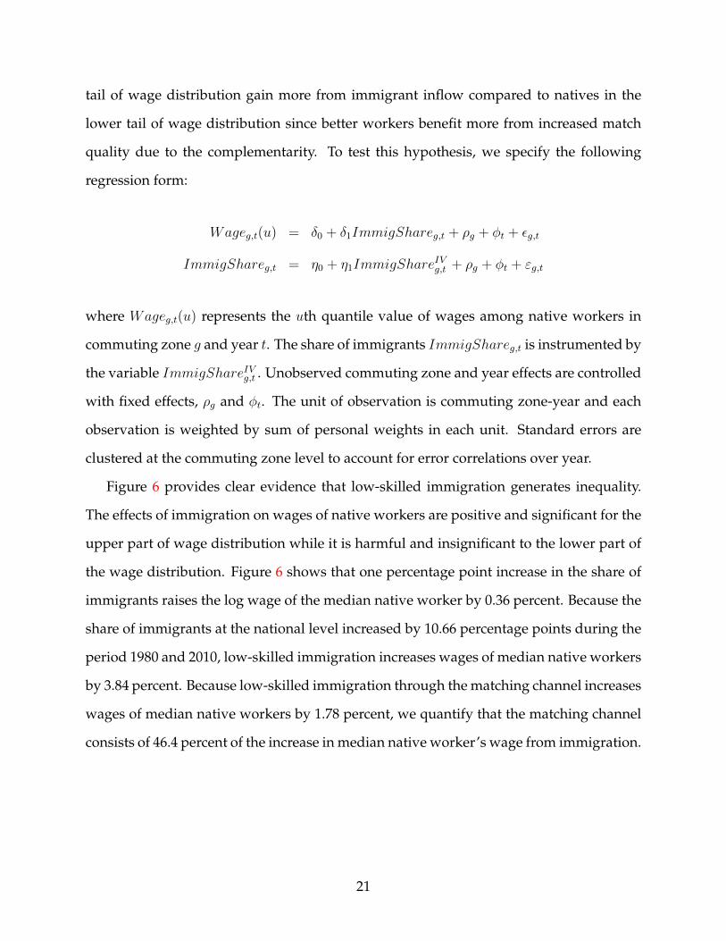
5.2.3 The effect of immigrant inflow on wage

We now examine whether the increase in match quality of natives leads to differential

effects on wages of heterogeneous native workers. We expect that natives in the upper

20

tail of wage distribution gain more from immigrant inflow compared to natives in the

lower tail of wage distribution since better workers benefit more from increased match

quality due to the complementarity. To test this hypothesis, we specify the following

regression form:

Wageg,t(u) = δ0 + δ1ImmigShareg,t + ρg + φt + εg,t

ImmigShareg,t = η0 + η1ImmigShareIVg,t + ρg + φt + εg,t

where Wageg,t(u) represents the uth quantile value of wages among native workers in

commuting zone g and year t. The share of immigrants ImmigShareg,t is instrumented by

the variable ImmigShareIVg,t . Unobserved commuting zone and year effects are controlled

with fixed effects, ρg and φt. The unit of observation is commuting zone-year and each

observation is weighted by sum of personal weights in each unit. Standard errors are

clustered at the commuting zone level to account for error correlations over year.

Figure 6 provides clear evidence that low-skilled immigration generates inequality.

The effects of immigration on wages of native workers are positive and significant for the

upper part of wage distribution while it is harmful and insignificant to the lower part of

the wage distribution. Figure 6 shows that one percentage point increase in the share of

immigrants raises the log wage of the median native worker by 0.36 percent. Because the

share of immigrants at the national level increased by 10.66 percentage points during the

period 1980 and 2010, low-skilled immigration increases wages of median native workers

by 3.84 percent. Because low-skilled immigration through the matching channel increases

wages of median native workers by 1.78 percent, we quantify that the matching channel

consists of 46.4 percent of the increase in median native worker’s wage from immigration.

21

6 Conclusion

This paper introduces a novel channel - a matching between workers and firms - to the lit-

erature on the effect of immigrants on wages and inequality of natives in the destination

country. Based on the matching framework adopted from the assignment framework

in trade literature and observations in the U.S. labor market, we construct a theoreti-

cal model where the influx of immigrants affects heterogeneous native workers through

the worker-firm re-matching channel. Low-skilled immigrants push natives up to be

matched with better firms, and due to the complementarity between worker skill and

firm productivity, the re-matching benefits better workers more and leads to an increase

in inequality.

Data show that immigrants in the U.S. tend to have lower skills than native workers.

Using the U.S. data from 1980 to 2010 and exploiting the variation in immigrant share

across commuting zones and years, we investigate whether our theoretical model can

explain the change in the inequality of natives from the inflow of low-skilled immigra-

tion. First, we have shown that immigration increases inequality in the U.S. Next, we

test whether the inflow of immigrants changes the matching and wages of native work-

ers. Consistent with our theory, natives are matched to more productive firms due to the

inflow of immigrants, and better native workers benefit more than other natives, which

explains why immigration leads to widening inequality in the U.S.

22

7 Appendix

7.1 Proofs

7.1.1 Proof of Proposition 1

Proof. Prove first that the matching function,m(z), and do not change. Rearranging equa-

tion (2) yields,

lnw(z) = − ln

(σ

σ − 1

)+σ − 1

σlnψ(m(z), z) +

1

σlnX − 1

σln

NH ′(z)

MG′(m(z))m′(z), (5)

By differentiating both equations with respect to z, we obtain the following second-order

differential equation for the matching function m(z):

m′′(z)

m′(z)= (σ − 1)

ψϕ(m(z), z)

ψ(m(z), z)− σψz(m(z), z)

ψ(m(z), z)+G′′(m(z))m′(z)

G′(m(z))− H ′′(z)

H ′(z), (6)

In equation (6), the matching function does not depend on the number of workersN . This

implies that the matching function, m(z), does not change. In equation (5), one percent

increase in N is associated with 1σ

percent decrease in wage function w(z) ∀z. Also, one

percent increase in X is associated with 1σ

percent increase in wage function w(z) ∀z.

One percent increase in N is associated with one percent increase in X . Hence, the wage

function, w(z), does not change.

7.1.2 Proof of Proposition 2

Proof. (i) Suppose that there exists z ∈ [zmin, zmax] such that m′(z) < m(z).h′(z′)

h′(z)≤

h(z′)

h(z)and the positive assortative matching property of the matching function imply that

m(zmin) = ϕmin ≤ m′(zmin) and m′(zmax) = ϕmax ≥ m(zmax). So there must exist zmin ≤

23

z1 ≤ z2 ≤ zmax and ϕmin ≤ ϕ1 ≤ ϕ2 ≤ ϕmax such that

i) m(z1) = m′(z1) = ϕ1 and m(z2) = m′(z2) = ϕ2,

ii) mz(z1) ≥ m′z(z

1) and m′z(z2) ≥ mz(z

2),

iii) m(z) > m′(z) for all z ∈ (z1, z2).

mz(z1) ≥ m′z(z

1) and m′z(z2) ≥ mz(z

2) implies that:

mz(z1)

mz(z2)≥ m′z(z

1)

m′z(z2).

Using equation (2), we can derive the following inequality:

[w(z1)

w(z2)

]σh(z1)

h(z2)≥[w′(z1)

w′(z2)

]σh′(z1)

h′(z2).

h′(z2)

h′(z1)≤ h(z2)

h(z1)requires that:

w′(z2)

w′(z1)≥ w(z2)

w(z1).

However, this is a contradiction. Since m′(z) < m(z), it must be that

w′(z2)

w′(z1)<w(z2)

w(z1).

Consequently, ifh′(z′)

h′(z)≤ h(z′)

h(z), then m′(z) ≥ m(z) for all z ∈ [zmin, zmax].

(ii) From equation (1),

∫ z′

z

ψz(ϕ, z)

ψ(ϕ, z)dz =

∫ z′

z

w′(z)

w(z)dz.

The right-hand side is the measure of wage inequality, lnw(z′) − lnw(z). Since the pro-

ductivity function ψ(ϕ, z) is strictly log supermodular, m′(z) ≥ m(z) for all z ∈ [zmin, zmax]

24

implies that the left-hand side is weakly increasing for all z ∈ [zmin, zmax]. Consequently,

the wage inequality rises.

7.1.3 Proof of Proposition 3

Proof. (i) Suppose that there does not exist z∗ ∈ [zmin, zmax] such that m′(z) ≥ m(z) for

all z ∈ [zmin, z∗] and m′(z) ≤ m(z) for all z ∈ [z∗, zmax]. Since

h′(z′)

h′(z)≥ h(z′)

h(z)for all

z′ ≥ z ≥ z andh′(z′)

h′(z)≤ h(z′)

h(z)for all z > z′ ≥ z, the positive assortative matching property

of the matching function implies that m(zmin) = ϕmin ≤ m′(zmin) and m(zmax) = ϕmax ≥

m′(zmax). Hence there must exist zmin ≤ z0 < z1 < z2 ≤ zmax and ϕmin ≤ ϕ0 < ϕ1 < ϕ2 ≤

ϕmax such that

i) m′(z0) = m(z0) = ϕ0, m′(z1) = m(z1) = ϕ1 and mN(z2L) = mS(z2

L) = ϕ2,

ii) m′z(z0) ≤ mz(z

0), m′z(z1) ≥ mz(z

1) and mN′

(z2L) ≤ mS

′

(z2L),

iii) m′(z) < m(z) for all z ∈ (z0, z1) and m′(z) > m(z) for all z ∈ (z1, z2).

There are two possible cases: z1 < z and z1 ≥ z. Suppose that z1 < z. m′z(z0) ≤ mz(z0)

and m′z(z1) ≥ mz(z

1) implies that:

m′z(z1)

m′z(z0)≥ mz(z

1)

mz(z0).

Using equation (2), we can derive the following inequality:

[w(z0)

w(z1)

]σh(z0)

h(z1)≥[w′(z0)

w′(z1)

]σh′(z0)

h′(z1).

h′(z1)

h′(z0)≤ h(z1)

h(z0)requires that:

w′(z1)

w′(z0)≥ w(z1)

w(z0).

25

However, this is a contradiction. Since m′(z) < m(z) for all z ∈ (z0, z1), it must be that

w′(z1)

w′(z0)<w(z1)

w(z0).

Suppose that z1 ≥ z. m′z(z2) ≤ mz(z2) and m′z(z

1) ≥ mz(z1) implies that:

m′z(z1)

m′z(z2)≥ mz(z

1)

mz(z2).

Using equation (2), we can derive the following inequality:

[w(z2)

w(z1)

]σh(z2)

h(z1)≥[w′(z2)

w′(z1)

]σh′(z2)

h′(z1).

h′(z1)

h′(z2)≤ h(z1)

h(z2)requires that:

w′(z1)

w′(z2)≥ w(z1)

w(z2).

However, this is a contradiction. Since m′(z) > m(z) for all z ∈ (z1, z2), it must be that

w′(z1)

w′(z2)<w(z1)

w(z2).

Consequently, there exists a skill level z∗ such that m′(z) ≥ m(z) for all z ∈ [zmin, z∗], and

m′(z) ≤ m(z) for all z ∈ [z∗, zmax].

(ii) The proof is identical to that of Proposition 2 - (ii).

26

7.2 Figures and Tables

Figure 1: Education distributions of natives and immigrants

Notes: The figure plots cumulative distribution functions for natives and immigrants by years ofeducation. The blue line denotes natives who were born in the U.S. in age 18 to 64 while the redshort-dashed line represents immigrants who were born in a foreign country in age 18 to 64. The source ofdata is the US Census 2000.

27

Figure 2: Positive assortative matching between workers and firms

Notes: The figure shows the relation between firm’s productivity and average education level of workers(top) and the relation between firm’s productivity and average imputed log hourly wages of workers(bottom) in each commuting zone-industry pair. Firm’s productivity is estimated as in section 5.1.5 andwage is imputed with observable characteristics of each worker. Each circle indicates the commutingzone-industry pair, and the size of the circle and fitted line is weighted by the total number of workers.The source of data is the US Census 2000.

28

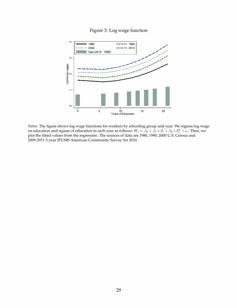
Figure 3: Log wage function

Notes: The figure shows log wage functions for workers by schooling group and year. We regress log wageon education and square of education in each year as follows: Wi = β0 + β1 ∗ Si + β2 ∗ S2

i + εi. Then, weplot the fitted values from the regression. The sources of data are 1980, 1990, 2000 U.S. Census and2009-2011 3-year IPUMS American Community Survey for 2010.

29

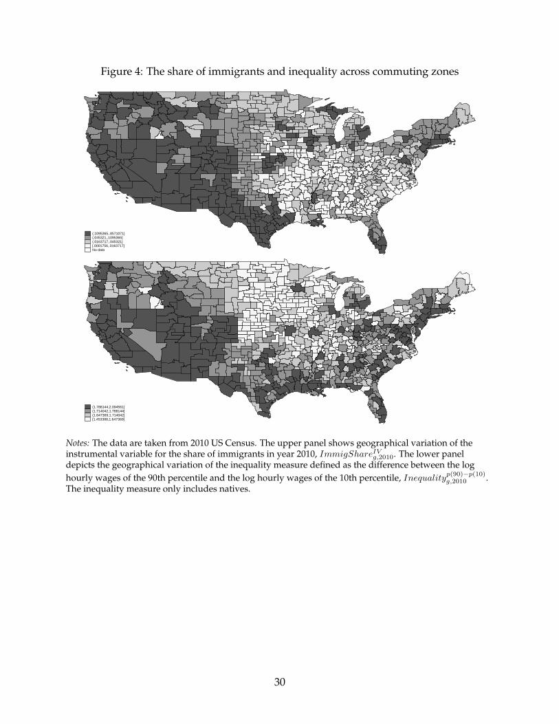
Figure 4: The share of immigrants and inequality across commuting zones

(.1095365,.8571071](.045321,.1095365](.0163717,.045321][.0001756,.0163717]No data

(1.788144,2.094561](1.714042,1.788144](1.647369,1.714042][1.453388,1.647369]

Notes: The data are taken from 2010 US Census. The upper panel shows geographical variation of theinstrumental variable for the share of immigrants in year 2010, ImmigShareIVg,2010. The lower paneldepicts the geographical variation of the inequality measure defined as the difference between the loghourly wages of the 90th percentile and the log hourly wages of the 10th percentile, Inequalityp(90)−p(10)

g,2010 .The inequality measure only includes natives.

30

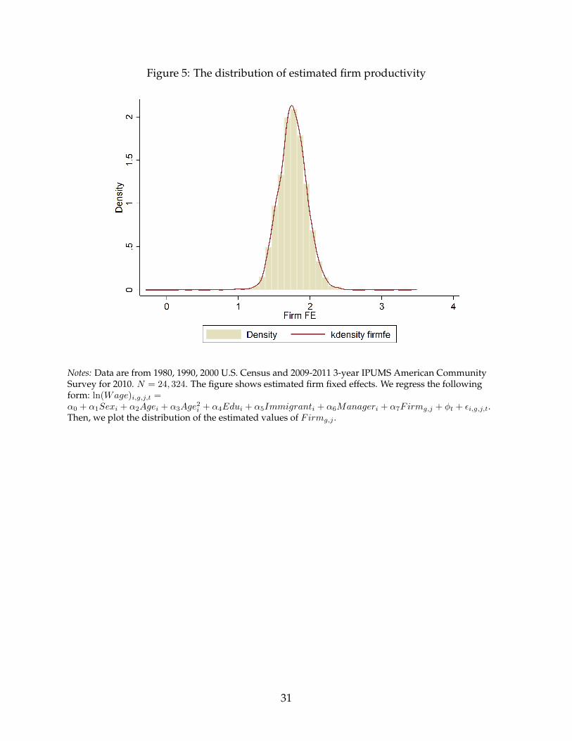
Figure 5: The distribution of estimated firm productivity

Notes: Data are from 1980, 1990, 2000 U.S. Census and 2009-2011 3-year IPUMS American CommunitySurvey for 2010. N = 24, 324. The figure shows estimated firm fixed effects. We regress the followingform: ln(Wage)i,g,j,t =α0 + α1Sexi + α2Agei + α3Age

2i + α4Edui + α5Immigranti + α6Manageri + α7Firmg,j + φt + εi,g,j,t.

Then, we plot the distribution of the estimated values of Firmg,j .

31

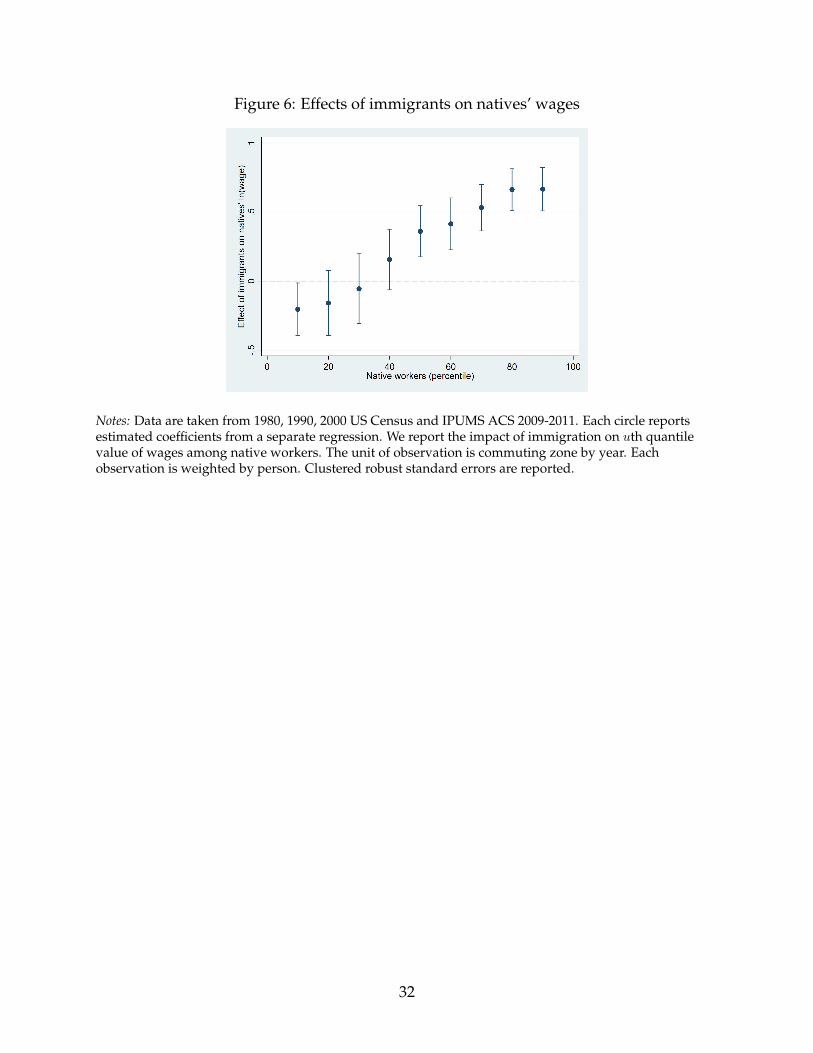
Figure 6: Effects of immigrants on natives’ wages

Notes: Data are taken from 1980, 1990, 2000 US Census and IPUMS ACS 2009-2011. Each circle reportsestimated coefficients from a separate regression. We report the impact of immigration on uth quantilevalue of wages among native workers. The unit of observation is commuting zone by year. Eachobservation is weighted by person. Clustered robust standard errors are reported.

32

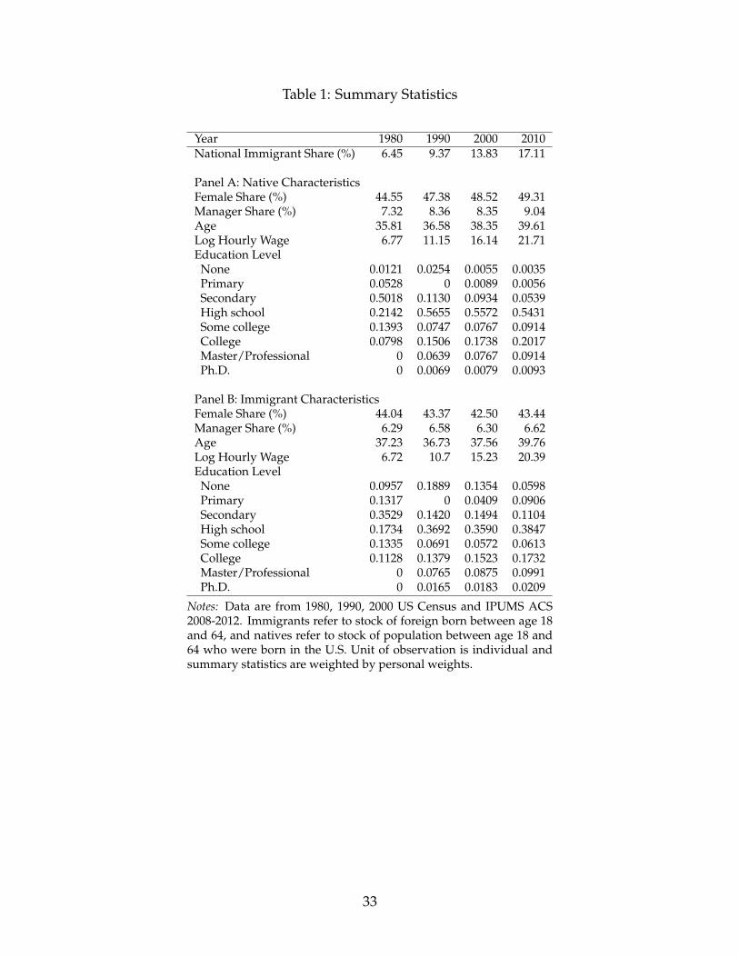
Table 1: Summary Statistics

Year 1980 1990 2000 2010National Immigrant Share (%) 6.45 9.37 13.83 17.11

Panel A: Native CharacteristicsFemale Share (%) 44.55 47.38 48.52 49.31Manager Share (%) 7.32 8.36 8.35 9.04Age 35.81 36.58 38.35 39.61Log Hourly Wage 6.77 11.15 16.14 21.71Education Level

None 0.0121 0.0254 0.0055 0.0035Primary 0.0528 0 0.0089 0.0056Secondary 0.5018 0.1130 0.0934 0.0539High school 0.2142 0.5655 0.5572 0.5431Some college 0.1393 0.0747 0.0767 0.0914College 0.0798 0.1506 0.1738 0.2017Master/Professional 0 0.0639 0.0767 0.0914Ph.D. 0 0.0069 0.0079 0.0093

Panel B: Immigrant CharacteristicsFemale Share (%) 44.04 43.37 42.50 43.44Manager Share (%) 6.29 6.58 6.30 6.62Age 37.23 36.73 37.56 39.76Log Hourly Wage 6.72 10.7 15.23 20.39Education Level

None 0.0957 0.1889 0.1354 0.0598Primary 0.1317 0 0.0409 0.0906Secondary 0.3529 0.1420 0.1494 0.1104High school 0.1734 0.3692 0.3590 0.3847Some college 0.1335 0.0691 0.0572 0.0613College 0.1128 0.1379 0.1523 0.1732Master/Professional 0 0.0765 0.0875 0.0991Ph.D. 0 0.0165 0.0183 0.0209

Notes: Data are from 1980, 1990, 2000 US Census and IPUMS ACS2008-2012. Immigrants refer to stock of foreign born between age 18and 64, and natives refer to stock of population between age 18 and64 who were born in the U.S. Unit of observation is individual andsummary statistics are weighted by personal weights.

33

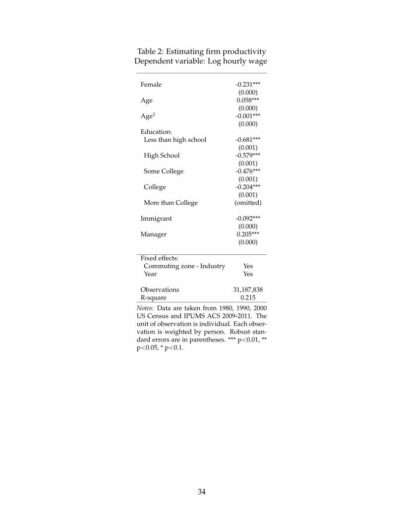
Table 2: Estimating firm productivityDependent variable: Log hourly wage

Female -0.231***(0.000)

Age 0.058***(0.000)

Age2 -0.001***(0.000)

Education:Less than high school -0.681***

(0.001)High School -0.579***

(0.001)Some College -0.476***

(0.001)College -0.204***

(0.001)More than College (omitted)

Immigrant -0.092***(0.000)

Manager 0.205***(0.000)

Fixed effects:Commuting zone - Industry YesYear Yes

Observations 31,187,838R-square 0.215

Notes: Data are taken from 1980, 1990, 2000US Census and IPUMS ACS 2009-2011. Theunit of observation is individual. Each obser-vation is weighted by person. Robust stan-dard errors are in parentheses. *** p<0.01, **p<0.05, * p<0.1.

34

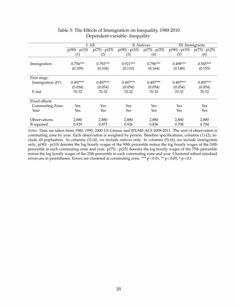
Table 3: The Effects of Immigration on Inequality, 1980-2010Dependent variable: Inequality

I. All II. Natives III. Immigrantsp(90) - p(10) p(75) - p(25) p(90) - p(10) p(75) - p(25) p(90) - p(10) p(75) - p(25)

(1) (2) (3) (4) (5) (6)

Immigration 0.754*** 0.792*** 0.921*** 0.796*** 0.498*** 0.545***(0.109) (0.104) (0.110) (0.164) (0.188) (0.155)

First stage:Immigration (IV) 0.497*** 0.497*** 0.497*** 0.497*** 0.497*** 0.497***

(0.054) (0.054) (0.054) (0.054) (0.054) (0.054)F stat 70.32 70.32 70.32 70.32 70.32 70.32

Fixed effects:Commuting Zone Yes Yes Yes Yes Yes YesYear Yes Yes Yes Yes Yes Yes

Observations 2,880 2,880 2,880 2,880 2,880 2,880R-squared 0.929 0.875 0.926 0.836 0.708 0.704

Notes: Data are taken from 1980, 1990, 2000 US Census and IPUMS ACS 2009-2011. The unit of observation iscommuting zone by year. Each observation is weighted by person. Baseline specifications, columns (1)-(2), in-clude all popluation. In columns (3)-(4), we include natives only. In columns (5)-(6), we include immigrantsonly. p(90) - p(10) denotes the log hourly wages of the 90th percentile minus the log hourly wages of the 10thpercentile in each commuting zone and year. p(75) - p(25) denotes the log hourly wages of the 75th percentileminus the log hourly wages of the 25th percentile in each commuting zone and year. Clustered robust standarderrors are in parentheses. Errors are clustered at commuting zone. *** p<0.01, ** p<0.05, * p<0.1.

35

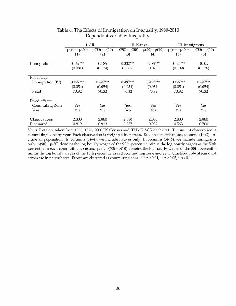
Table 4: The Effects of Immigration on Inequality, 1980-2010Dependent variable: Inequality

I. All II. Natives III. Immigrantsp(90) - p(50) p(50) - p(10) p(90) - p(50) p(50) - p(10) p(90) - p(50) p(50) - p(10)

(1) (2) (3) (4) (5) (6)

Immigration 0.569*** 0.185 0.332*** 0.589*** 0.525*** -0.027(0.081) (0.124) (0.065) (0.076) (0.109) (0.136)

First stage:Immigration (IV) 0.497*** 0.497*** 0.497*** 0.497*** 0.497*** 0.497***

(0.054) (0.054) (0.054) (0.054) (0.054) (0.054)F stat 70.32 70.32 70.32 70.32 70.32 70.32

Fixed effects:Commuting Zone Yes Yes Yes Yes Yes YesYear Yes Yes Yes Yes Yes Yes

Observations 2,880 2,880 2,880 2,880 2,880 2,880R-squared 0.819 0.913 0.757 0.939 0.563 0.700

Notes: Data are taken from 1980, 1990, 2000 US Census and IPUMS ACS 2009-2011. The unit of observation iscommuting zone by year. Each observation is weighted by person. Baseline specifications, columns (1)-(2), in-clude all popluation. In columns (3)-(4), we include natives only. In columns (5)-(6), we include immigrantsonly. p(90) - p(50) denotes the log hourly wages of the 90th percentile minus the log hourly wages of the 50thpercentile in each commuting zone and year. p(50) - p(10) denotes the log hourly wages of the 50th percentileminus the log hourly wages of the 10th percentile in each commuting zone and year. Clustered robust standarderrors are in parentheses. Errors are clustered at commuting zone. *** p<0.01, ** p<0.05, * p<0.1.

36

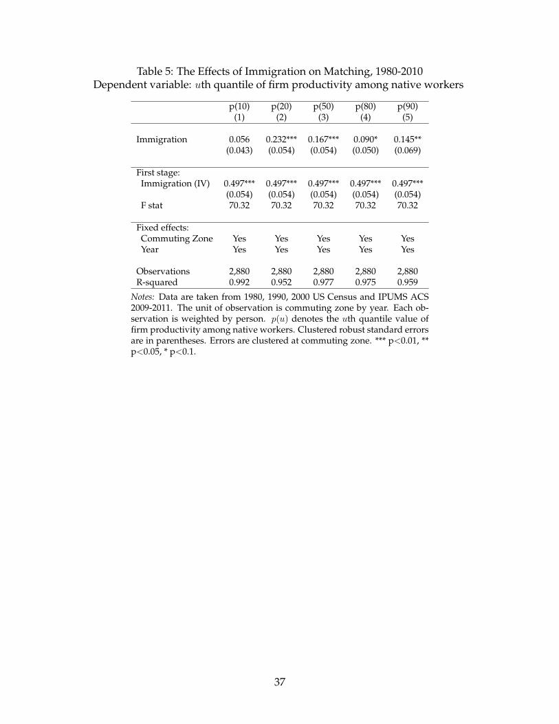
Table 5: The Effects of Immigration on Matching, 1980-2010Dependent variable: uth quantile of firm productivity among native workers

p(10) p(20) p(50) p(80) p(90)(1) (2) (3) (4) (5)

Immigration 0.056 0.232*** 0.167*** 0.090* 0.145**(0.043) (0.054) (0.054) (0.050) (0.069)

First stage:Immigration (IV) 0.497*** 0.497*** 0.497*** 0.497*** 0.497***

(0.054) (0.054) (0.054) (0.054) (0.054)F stat 70.32 70.32 70.32 70.32 70.32

Fixed effects:Commuting Zone Yes Yes Yes Yes YesYear Yes Yes Yes Yes Yes

Observations 2,880 2,880 2,880 2,880 2,880R-squared 0.992 0.952 0.977 0.975 0.959

Notes: Data are taken from 1980, 1990, 2000 US Census and IPUMS ACS2009-2011. The unit of observation is commuting zone by year. Each ob-servation is weighted by person. p(u) denotes the uth quantile value offirm productivity among native workers. Clustered robust standard errorsare in parentheses. Errors are clustered at commuting zone. *** p<0.01, **p<0.05, * p<0.1.

37

References

Antras, Pol, Luis Garicano, and Esteban Rossi-Hansberg, “Offshoring in a Knowledge

Economy,” Quarterly Journal of Economics, 2006, 121 (1), 31–77.

Autor, David H., David Dorn, and Gordon H. Hanson, “The China Syndrome: Local

Labor Market Effects of Import Competition in the United States,” American Economic

Review, 2013, 103 (6), 2121–68.

Basso, Gaetano and Giovanni Peri, “The Association between Immigration and Labor

Market Outcomes in the United States,” 2015.

Borjas, George J, “The Labor Demand Curve Is Downward Sloping: Reexamining the

Impact of Immigration on the Labor Market,” Quarterly Journal of Economics, 2003,

pp. 1335–1374.

Card, David, “Immigration and Inequality,” American Economic Review, 2009, 99 (2), 1–21.

Costinot, Arnaud and Jonathan Vogel, “Matching and Inequality in the World Econ-

omy,” Journal of Political Economy, 2010, 118 (4), 747–786.

Grossman, Gene M and Elhanan Helpman, “Growth, trade, and inequality,” Economet-

rica, 2018, 86 (1), 37–83.

, , and Philipp Kircher, “Matching, Sorting, and the Distributional Effects of Interna-

tional Trade,” Journal of Political Economy, 2017, 125 (1), 000–000.

Hunt, Jennifer and Marjolaine Gauthier-Loiselle, “How Much Does Immigration Boost

Innovation?,” American Economic Journal: Macroeconomics, 2010, pp. 31–56.

Kremer, Michael and Eric Maskin, “Wage inequality and segregation by skill,” Technical

Report, National Bureau of Economic Research 1996.

and , “Globalization and inequality,” Technical Report, Working Paper 2006.

38

Lemieux, Thomas, “Postsecondary Education and Increasing Wage Inequality,” American

Economic Review, 2006, pp. 195–199.

, “The changing nature of wage inequality,” Journal of Population Economics, 2008, 21 (1),

21–48.

Ohnsorge, Franziska and Daniel Trefler, “Sorting It Out: International Trade with Het-

erogeneous Workers,” Journal of Political Economy, 2007, 115 (5), 868–892.

Ortega, Francesc and Giovanni Peri, “Openness and income: The roles of trade and

migration,” Journal of International Economics, 2014, 92 (2), 231–251.

Ottaviano, Gianmarco IP and Giovanni Peri, “Rethinking the effect of immigration on

wages,” Journal of the European economic association, 2012, 10 (1), 152–197.

Peri, Giovanni, “Immigrants, Productivity, and Labor Markets,” Journal of Economic Per-

spectives, 2016, 30 (4), 3–29.

and Chad Sparber, “Task Specialization, Immigration, and Wages,” American Economic

Journal: Applied Economics, 2009, 1 (3), 135–69.

Sampson, Thomas, “Selection into trade and wage inequality,” American Economic Jour-

nal: Microeconomics, 2014, 6 (3), 157–202.

Tolbert, Charles M and Molly Sizer, “US commuting zones and labor market areas: A

1990 update,” 1996.

39