image classification using convolutional neural …...image classification using convolutional...

International Journal of Advancements in Research & Technology, Volume 3, Issue 6, June-2014 1661 ISSN 2278-7763

IJSER © 2014

http://www.ijser.org

Image Classification Using Convolutional Neural Networks

Deepika Jaswal, Sowmya.V, K.P.Soman

Abstract—Deep Learning has emerged as a new area in machine learning and is applied to a number of signal and image

applications.The main purpose of the work presented in this paper, is to apply the concept of a Deep Learning algorithm namely,

Convolutional neural networks (CNN) in image classification. The algorithm is tested on various standard datasets, like remote sensing

data of aerial images (UC Merced Land Use Dataset) and scene images from SUN database. The performance of the algorithm is

evaluated based on the quality metric known as Mean Squared Error (MSE) and classification accuracy. The graphical representation of

the experimental results is given on the basis of MSE against the number of training epochs. The experimental result analysis based on the

quality metrics and the graphical representation proves that the algorithm (CNN) gives fairly good classification accuracy for all the tested

datasets.

Index Terms—Deep Learning, Convolutional neural networks, Image Classification, Scene Classification, Aerial image classification.

—————————— ——————————

1 INTRODUCTION

Lillsand and Kiefer defined image processing as involving manipulation of digital images with the use of computer. It is a broad subject and involves processes that are mathematically complex [1]. Image processing involves some basic operations namely image restoration/rectification, image enhancement, image classification, images fusion etc. Image classification forms an important part of image processing. The objective of image classification is the automatic allocation of image to thematic classes [1]. Two types of classification are supervised classification and unsupervised classification. The process of image classification involves two steps, training of the system followed by testing. The training process means, to take the characteristic properties of the images (form a class) and form a unique description for a particular class. The process is done for all classes depending on the type of classi-fication problem; binary classification or multi-class classifica-tion. The testing step means to categorize the test images un-der various classes for which system was trained. This assign-ing of class is done based on the partitioning between classes based on the training features. Since 2006, deep structured learning, or more commonly called deep learning or hierarchical learning, has emerged as a new area of machine learning research [2]. Several definitions are available for Deep Learning; coating one of the many defi-nitions from [2] Deep Learning is defined as: A class of ma-chine learning techniques that exploit many layers of non-linear information processing for supervised or unsupervised feature extraction and transformation and for pattern analysis and classification. This work aims at the application of Convolutional Neural Network or CNN for image classification. The image data used for testing the algorithm includes remote sensing data of aerial images and scene data from SUN database [12] [13] [14]. The rest of the paper is organized as follows. Section 2 deals with the working of the network followed by section 2.1 with theoretical background. The working of CNN is described in section 2.2. Section 3 gives the experimental procedure in de-tail. Finally, section 4 deals with the experimental results ob-tained using CNN.

2 WORKING OF THE NETWORK

Working of the network is divided into two sections. Section 2.1 defines about the theory related to CNN in a brief manner. Section 2.2 deals with the properties of CNN and the function of layers.

2.1 Theoritical Background

Computational models of neural networks have been around for a long time, first model proposed was by McCulloch and Pitts as in [3]. Neural networks are made up of a number of layers with each layer connected to the other layers forming the network. A feed-forward neural network or FFNN can be thought of in terms of neural activation and the strength of the connections between each pair of neurons [4] In FFNN, the neurons are connected in a directed way having clear start and stop place i.e., the input layer and the output layer. The layer between these two layers, are called as the hidden layers. Learning occurs through adjustment of weights and the aim is to try and minimize error between the output obtained from the output layer and the input that goes into the input layer. The weights are adjusted by process of back prop-agation (in which the partial derivative of the error with re-spect to last layer of weights is calculated). The process of weight adjustment is repeated in a recursive manner until weight layer connected to input layer is updated.

Figure 1: Typical network architecture [4]

IJSER


IJSER © 2014


Convolutional Neural Networks (CNN) is variants of Multi- Layer Perceptron (MLPs) which are inspired from biology. These filters are local in input space and are thus better suited to exploit the strong spatially local correlation present in natu-ral images [5]. Convolutional neural networks are designed to process two-dimensional (2-D) image [6]. A CNN architecture used in this project is that defined in [7]. The network consists of three types of layers namely convolution layer, sub sam-pling layer and the output layer.

2.2 Working of CNN algorithm

This section explains the working of the algorithm in a brief manner. The detailed explanation is available in [7]. The input to the network is a 2D image. The network has in-put layer which takes the image as the input, output layer from where we get the trained output and the intermediate layers called as the hidden layers. As stated earlier, the net-work has a series of convolutional and sub-sampling layers. Together the layers produce an approximation of input image data’s. CNNs exploit spatially local correlation by enforcing a local connectivity pattern between neurons of adjacent layers [8]. Neurons in layer say, ‘m’ are connected to a local subset of neurons from the previous layer of (m-1), where the neurons of the (m-1) layer have contiguous receptive fields, as shown in figure (2a).

Figure 2(a): Graphical flow of layers showing connection between layers [4]

Figure 2(b): Graphical flow of layers showing sharing of weights [4]

In the CNN algorithm, each sparse filter is replicated across the entire visual field. These units then form a feature maps, these share weight vector and bias. Figure (2b), represents three hidden units of same feature map. The weights of same color are shared, thus constrained to be identical.

----------------------------------------------------

The gradient of shared weights is the sum of the gradients of the parameters being shared. Such replication in a way allows features to be detected regardless of their position in visual field. In addition to this, weight sharing also allows to reduce the number of free learning parameters. Due to this control, CNN tends to achieve better generalization on vision prob-lems. CNN also make use of the concept of max-pooling, which is a form of non-linear down-sampling. In this method, the input image is partitioned into non-overlapping rectangles. The output for each sub-region is the maximum value.

2.2.1 Convolution layer

The convolution layer is the first layer of the CNN network. The structure of this layer is shown in the figure (3). It consists of a convolution mask, bias terms and a function expression. Together, these generate output of the layer. The figure below shows a 5x5 mask that perform convolution over a 32x32 input feature map. The resultant output is a 28x28 matrix. Then bias is added and sigmoid function is ap-plied on the matrix [7].

Figure 3: Convolutional layer working [7]

2.2.2 Sub sampling layer

The sub sampling layer comes after the convolutional layer. It has same number of planes as the convolutional layer. The purpose of this layer is to reduce the size of the feature map. It divides the image into blocks of 2x2 and performs averaging. Sub sampling layer preserves the relative information between features and not the exact relation.

Figure 4: Sub sampling layer working [7]

Deepika Jaswal is currently pursuing masters degree program inRemote

sensing and wireless sensor network in Amrita University, India. E-mail:

[email protected]

Sowmya.V is Assistant Professor, CEN department Amrita University,

India. E-mail: [email protected]

Dr.K.P.Soman is Professor and Head of Department, CEN Department,

Amrita University, India.

IJSER


IJSER © 2014


3 EXPERIMENTAL PROCEDURE

3.1 Preparing Database

The input is given as image itself. The images are converted to gray scale as data information is important for the network and not the color information. Also, the images are resized to 32x32. Since the images from data sets are larger, pyramid reduction is done to make them of 32x32 in size. The image pyramid is a data structure designed to support efficient scaled convolution through reduced image representation. It consists of a sequence of copies of an original image in which both sample density and resolution are decreased in regular steps [9]. 3.1 Network training and testing

The purpose of training algorithm as in [7] is to train a net-work such that the error is minimized between the network output and the desired output. The error function is as defined by the equation below and is same for weights as well as bias terms.

2

1 1

1( ) ( )

LNKk kn n

k n

E w y dK N

Here k

nyis the actual output of the network, K is the number

of input image and the output vectors desired. kx be the

thk training image and kd corresponding desired output vec-

tor. The error gradient is computed through error sensitivi-

ties, which are defined as the partial derivatives of the error

function with respect to the weighted sum input to a neuron.

Once the error gradient ∇E(t) is derived, numerous optimiza-

tion algorithms for minimizing the energy function can be

applied to train the network. Here RPROP (resilient back

propagation) is used. It is an efficient learning scheme that

performs a direct adaptation of the weight step based on local

gradient information [10].

4 RESULTS AND DISSCUSSION

This section presents the result of the classification accuracies obtained using CNN algorithm on various standard datasets. The results are presented using the classification accuracy in percentage for within train data and test data separately. Along with the classification accuracy percentage values, MSE (Mean Squared Error) graph is also presented. The Graphs show the change of MSE with respect to the training epochs. MSE metric is the simplest and widely used quality metric. It is the mean of the squared difference between original and trained approximation. A better trained image will result in lower MSE with the origi-nal image. As the value for Mean Squared Error (MSE) tends to decrease, the variation in the final reconstructed output and the original image is very less. MSE indicates the close prox-imity between underlying true image and the final recon-structed output. The idea here is to use enough number of epochs that would result in low MSE, high classification accu-

racy and with least duration for training the network. The network is tested on various datasets, in turn each da-

taset is tested for different number of iterations (epochs). Sec-tion 4.1 presents the result of face image versus non-face im-age classification. The experiment from [7] is repeated to study the various network parameters and their effect on network outputs. The algorithm was tested on aerial images, results of which are presented in section 4.2. Section 4.3 presents results obtained for scene classification images. 4.1 Face vs. Non-face Image Classification

The data used in this experiment are taken from a face and skin detection database [11]. 1000 face images and 1000 non-face images are used for training and testing the network. The images are of 32 × 32 pixels. Some sample images are shown in figure (5).

Figure 6(a), 6(b) and 6(c) show variation of MSE for 200, 300 and 500 epochs respectively. From the graphs below, we infer that the MSE reduces considerably as the epoch value changes from 200 to 300. However, the MSE value undergoes mini-mum variation, as we change the number of epochs from 300 to 500.

Figure 6(a): Variation of MSE for face vs. non-face images (200 epochs)

IJSER


IJSER © 2014


Figure 6(b): Variation of MSE for face vs. non-face images (300 epochs)

Figure 6(c): Variation of MSE for face vs. non-face images (500 epochs)

The same observation is also obtained from the classification accuracy values where, accuracy improves as we move from 200 to 300 epochs. But, there is very less change as we change the epoch from 300 to 500. Thus, result for 300 epochs is se-lected, as it is best suited and better than 200 epochs and simi-lar to the result of 500 epoch result. The computational cost involved in the result for 200 epochs is comparatively very low, when compared with that of the 500 epochs. Classifica-tion accuracy for train data (300 epochs) is 95.90% and the classification accuracy for train data (300 epochs) is 92.78%. 4.2 Face vs. Non-face Image Classification

The CNN algorithm is applied to set of aerial dataset and test-ed for its classification accuracy. The dataset used is UC Merced Land Use Dataset [12]. This is a 21 class land use image dataset meant for research purposes. There are 100 images for each class. Each image measures 256x256 pixels. The images were manually extracted from large images from the USGS National Map Urban Area Imagery collection for various urban areas around the coun-try. The pixel resolution of this public domain imagery is 1 foot. The classification is done between two sets of data at a time. And the results were evaluated using classification accu-racy for train and test data as well as MSE curves for different epochs used.

Figure (7) below shows sample images of the classes used from the aerial dataset.

Figure 7: Sample of Buildings, Agricultural, Dense residential and Forest

4.2.1 Building vs. Agricultural images

The first test is done on aerial images of building versus agri-cultural fields. From the sample images in figure (8), it is seen that the two classes are very distinct and the algorithm gives high classification accuracy. The below graph in figure (8) shows that the network is trained within 250 epochs to give the classification accuracy for train data as 93.50% and test data as 90.00%.

Figure 8: Variation of MSE. for Building vs. Agricultural imaes (250 epochs)

4.2.2 Dense residential vs. Forest

The images for dense residential are those of roof tops, row housing and interleaving streets, while, forest images are those of tree tops shown in figure (7) These set of distinct images gives high classification accuracy

IJSER


IJSER © 2014


of 93.50% on train data. The MSE graph presented in figure (9) shows low MSE is achieved in 250 epochs.

Figure 9: Variation of MSE for Dense residential images vs. forest images (250 epochs)

4.2.3 Dense residential vs. Agricultural

Dense residential images versus agricultural images present yet another set of distinct images. A high classification accura-cy of 91.50% is obtained on the train data. figure (10) shows the MSE graph for 250 epochs.

Figure 10: Variation of MSE for Dense residential vs.

agricultural images (250 epochs)

4.2.4 Consturcted regions vs. Green regions

This dataset is prepared by clubbing the building images with the dense residential images as ‘Constructed’ features. ‘Green’ features comprise of agricultural and forest class images. High classification accuracy of 97.00% is obtained. Figure (11) shows the variation of MSE for 350 epochs.

Figure 11: Variation of MSE for Constructed region images vs. green region images (350 epochs)

4.2.5 Agricultural vs. Forest

Agricultural images are those of open fields and tree tops. Forest images are of tree tops and few open spaces. These set of images are similar. As a result, the classification accuracy reduces to 77%. Figure (12) below shows the MSE graph for 250 epochs.

Figure 12: Variation of MSE for Agricultural images vs. forest

images (250 epochs)

4.2.6 Building vs. Dense residential

The images for building are those of roof tops, row housing and interleaving streets. Images for dense residential also con-tain similar information. Thus the classification accuracy is low (57%) for these two classes. Figure (13) below shows the MSE graph for 250 epochs.

IJSER


IJSER © 2014


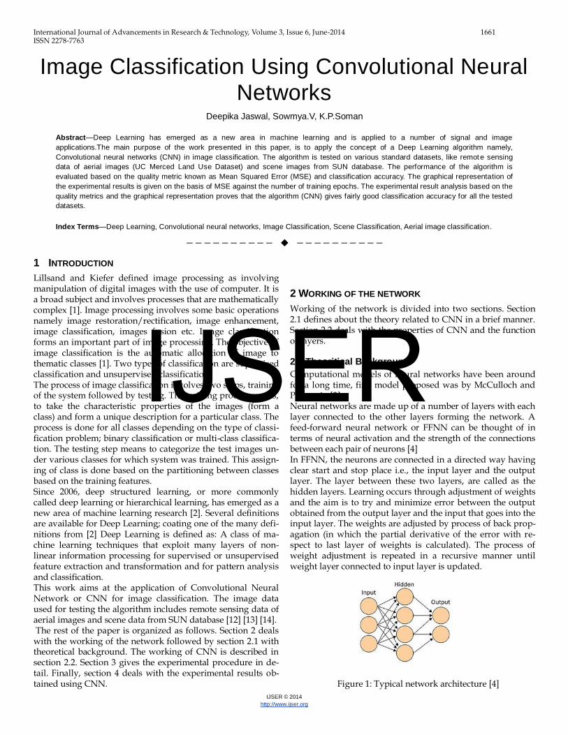
Figure 13: Variation of MSE for building images vs. dense res-

idential images (250 epochs)

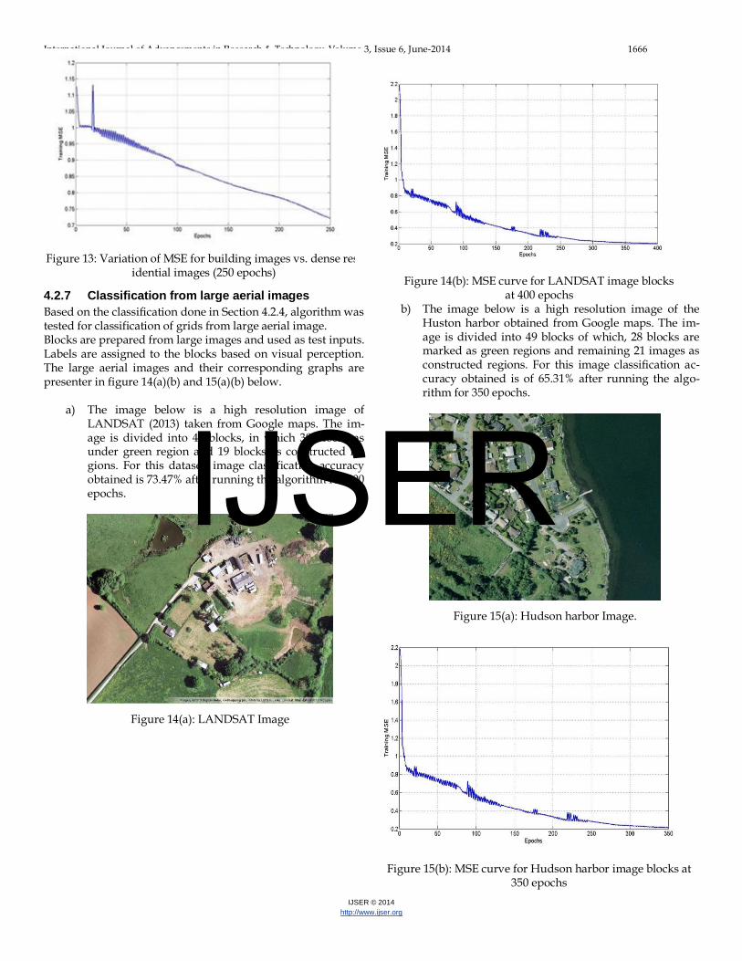
4.2.7 Classification from large aerial images

Based on the classification done in Section 4.2.4, algorithm was tested for classification of grids from large aerial image. Blocks are prepared from large images and used as test inputs. Labels are assigned to the blocks based on visual perception. The large aerial images and their corresponding graphs are presenter in figure 14(a)(b) and 15(a)(b) below.

a) The image below is a high resolution image of LANDSAT (2013) taken from Google maps. The im-age is divided into 49 blocks, in which 30 blocks as under green region and 19 blocks as constructed re-gions. For this dataset, image classification accuracy obtained is 73.47% after running the algorithm for 400 epochs.

Figure 14(a): LANDSAT Image

Figure 14(b): MSE curve for LANDSAT image blocks at 400 epochs

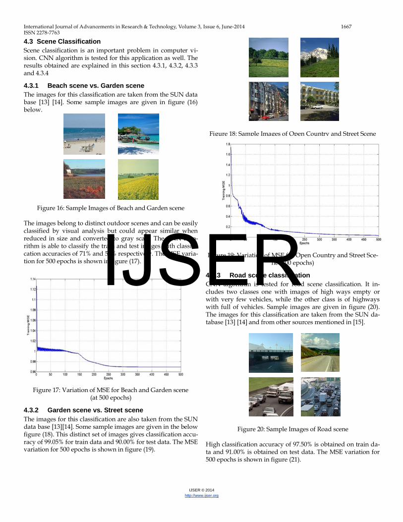
b) The image below is a high resolution image of the Huston harbor obtained from Google maps. The im-age is divided into 49 blocks of which, 28 blocks are marked as green regions and remaining 21 images as constructed regions. For this image classification ac-curacy obtained is of 65.31% after running the algo-rithm for 350 epochs.

Figure 15(a): Hudson harbor Image.

Figure 15(b): MSE curve for Hudson harbor image blocks at 350 epochs

IJSER


IJSER © 2014


4.3 Scene Classification

Scene classification is an important problem in computer vi-sion. CNN algorithm is tested for this application as well. The results obtained are explained in this section 4.3.1, 4.3.2, 4.3.3 and 4.3.4

4.3.1 Beach scene vs. Garden scene

The images for this classification are taken from the SUN data base [13] [14]. Some sample images are given in figure (16) below.

Figure 16: Sample Images of Beach and Garden scene The images belong to distinct outdoor scenes and can be easily classified by visual analysis but could appear similar when reduced in size and converted to gray scale. The CNN algo-rithm is able to classify the train and test images with classifi-cation accuracies of 71% and 51% respectively. The MSE varia-tion for 500 epochs is shown in figure (17).

Figure 17: Variation of MSE for Beach and Garden scene

(at 500 epochs)

4.3.2 Garden scene vs. Street scene

The images for this classification are also taken from the SUN data base [13][14]. Some sample images are given in the below figure (18). This distinct set of images gives classification accu-racy of 99.05% for train data and 90.00% for test data. The MSE variation for 500 epochs is shown in figure (19).

Figure 18: Sample Images of Open Country and Street Scene

Figure 19: Variation of MSE for Open Country and Street Sce-

ne (500 epochs)

4.3.3 Road scene classification

CNN algorithm is tested for road scene classification. It in-cludes two classes one with images of high ways empty or with very few vehicles, while the other class is of highways with full of vehicles. Sample images are given in figure (20). The images for this classification are taken from the SUN da-tabase [13] [14] and from other sources mentioned in [15].

Figure 20: Sample Images of Road scene High classification accuracy of 97.50% is obtained on train da-ta and 91.00% is obtained on test data. The MSE variation for 500 epochs is shown in figure (21).

IJSER


IJSER © 2014


Figure 21: Variation of MSE for Road scene classification

(300 epochs)

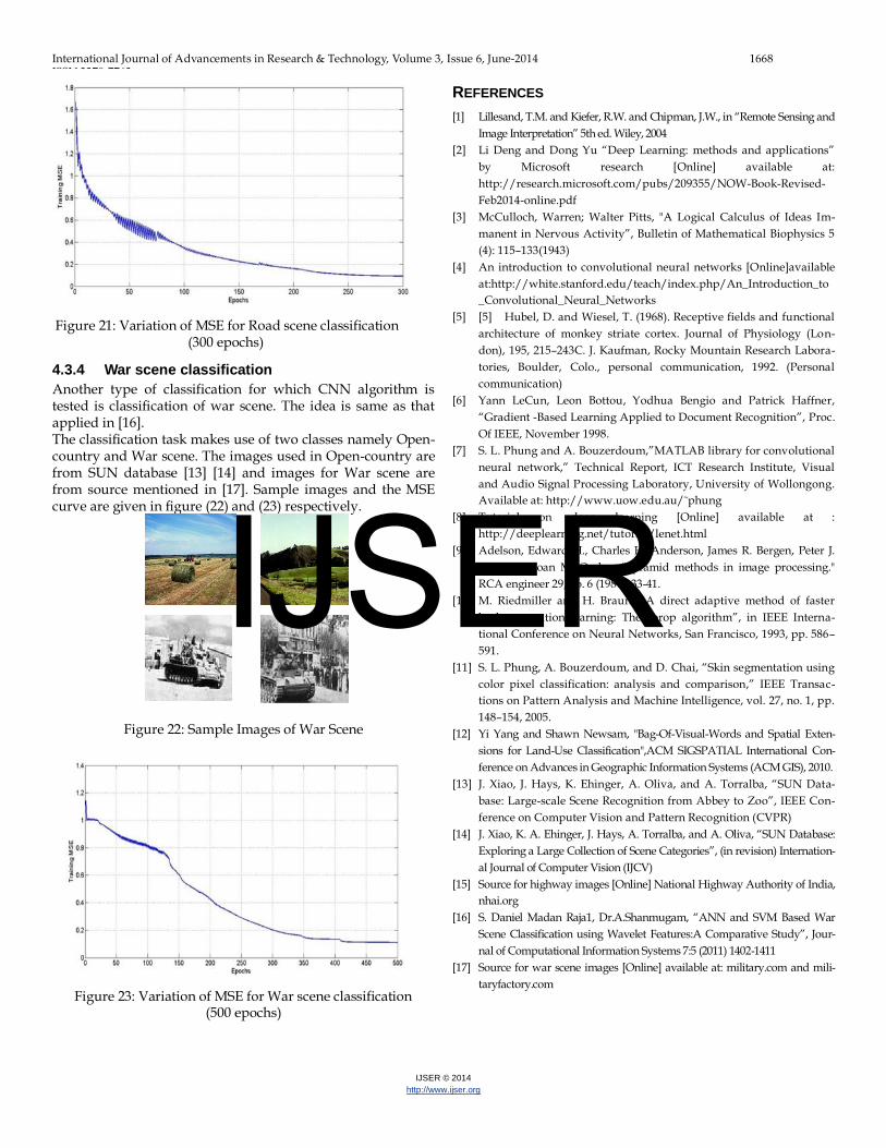
4.3.4 War scene classification

Another type of classification for which CNN algorithm is tested is classification of war scene. The idea is same as that applied in [16]. The classification task makes use of two classes namely Open-country and War scene. The images used in Open-country are from SUN database [13] [14] and images for War scene are from source mentioned in [17]. Sample images and the MSE curve are given in figure (22) and (23) respectively.

Figure 22: Sample Images of War Scene

Figure 23: Variation of MSE for War scene classification

(500 epochs)

REFERENCES

[1] Lillesand, T.M. and Kiefer, R.W. and Chipman, J.W., in “Remote Sensing and

Image Interpretation” 5th ed. Wiley, 2004

[2] Li Deng and Dong Yu “Deep Learning: methods and applications”

by Microsoft research [Online] available at:

http://research.microsoft.com/pubs/209355/NOW-Book-Revised-

Feb2014-online.pdf

[3] McCulloch, Warren; Walter Pitts, "A Logical Calculus of Ideas Im-

manent in Nervous Activity”, Bulletin of Mathematical Biophysics 5

(4): 115–133(1943)

[4] An introduction to convolutional neural networks [Online]available

at:http://white.stanford.edu/teach/index.php/An_Introduction_to

_Convolutional_Neural_Networks

[5] [5] Hubel, D. and Wiesel, T. (1968). Receptive fields and functional

architecture of monkey striate cortex. Journal of Physiology (Lon-

don), 195, 215–243C. J. Kaufman, Rocky Mountain Research Labora-

tories, Boulder, Colo., personal communication, 1992. (Personal

communication)

[6] Yann LeCun, Leon Bottou, Yodhua Bengio and Patrick Haffner,

“Gradient -Based Learning Applied to Document Recognition”, Proc.

Of IEEE, November 1998.

[7] S. L. Phung and A. Bouzerdoum,”MATLAB library for convolutional

neural network,” Technical Report, ICT Research Institute, Visual

and Audio Signal Processing Laboratory, University of Wollongong.

Available at: http://www.uow.edu.au/˜phung

[8] Tutorial on deep learning [Online] available at :

http://deeplearning.net/tutorial/lenet.html

[9] Adelson, Edward H., Charles H. Anderson, James R. Bergen, Peter J.

Burt, and Joan M. Ogden. "Pyramid methods in image processing."

RCA engineer 29, no. 6 (1984): 33-41.

[10] M. Riedmiller and H. Braun, “A direct adaptive method of faster

backpropagation learning: The rprop algorithm”, in IEEE Interna-

tional Conference on Neural Networks, San Francisco, 1993, pp. 586–

591.

[11] S. L. Phung, A. Bouzerdoum, and D. Chai, “Skin segmentation using

color pixel classification: analysis and comparison,” IEEE Transac-

tions on Pattern Analysis and Machine Intelligence, vol. 27, no. 1, pp.

148–154, 2005.

[12] Yi Yang and Shawn Newsam, "Bag-Of-Visual-Words and Spatial Exten-

sions for Land-Use Classification",ACM SIGSPATIAL International Con-

ference on Advances in Geographic Information Systems (ACM GIS), 2010.

[13] J. Xiao, J. Hays, K. Ehinger, A. Oliva, and A. Torralba, “SUN Data-

base: Large-scale Scene Recognition from Abbey to Zoo”, IEEE Con-

ference on Computer Vision and Pattern Recognition (CVPR)

[14] J. Xiao, K. A. Ehinger, J. Hays, A. Torralba, and A. Oliva, “SUN Database:

Exploring a Large Collection of Scene Categories”, (in revision) Internation-

al Journal of Computer Vision (IJCV)

[15] Source for highway images [Online] National Highway Authority of India,

nhai.org

[16] S. Daniel Madan Raja1, Dr.A.Shanmugam, “ANN and SVM Based War

Scene Classification using Wavelet Features:A Comparative Study”, Jour-

nal of Computational Information Systems 7:5 (2011) 1402-1411

[17] Source for war scene images [Online] available at: military.com and mili-

taryfactory.com

IJSER

image classification using convolutional neural …...image classification using convolutional...

Documents