7

II. CONSERVATION ASSESSMENT

Colorado Division of Wildlife, Kathleen Tadvick, April 2007

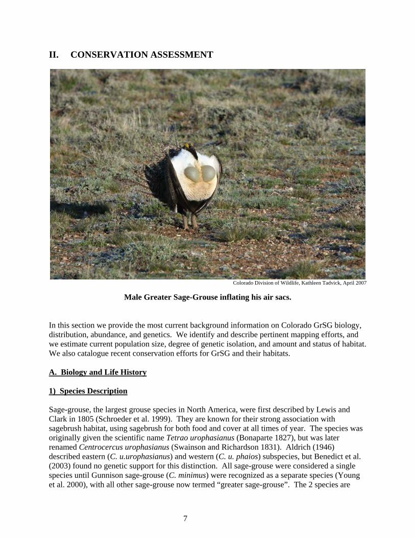
Male Greater Sage-Grouse inflating his air sacs.

In this section we provide the most current background information on Colorado GrSG biology, distribution, abundance, and genetics. We identify and describe pertinent mapping efforts, and we estimate current population size, degree of genetic isolation, and amount and status of habitat. We also catalogue recent conservation efforts for GrSG and their habitats. A. Biology and Life History 1) Species Description Sage-grouse, the largest grouse species in North America, were first described by Lewis and Clark in 1805 (Schroeder et al. 1999). They are known for their strong association with sagebrush habitat, using sagebrush for both food and cover at all times of year. The species was originally given the scientific name Tetrao urophasianus (Bonaparte 1827), but was later renamed Centrocercus urophasianus (Swainson and Richardson 1831). Aldrich (1946) described eastern (C. u.urophasianus) and western (C. u. phaios) subspecies, but Benedict et al. (2003) found no genetic support for this distinction. All sage-grouse were considered a single species until Gunnison sage-grouse (C. minimus) were recognized as a separate species (Young et al. 2000), with all other sage-grouse now termed “greater sage-grouse”. The 2 species are

8

differentiated morphologically, by size (Hupp and Braun 1991, Young et al. 2000) and plumage (Young et al. 2000), genetically (Kahn et al. 1999, Oyler-McCance et al. 1999), and behaviorally by differences in strutting behavior (Barber 1991, Young 1994, Young et al. 2000). The current ranges of the 2 species are not overlapping or adjacent (Schroeder et al. 2004). Greater sage-grouse are sexually dimorphic in size and plumage. Adult males weigh 5.5 – 7.0 pounds, adult females are 2.9 – 3.8 pounds, yearling males range from 4.9 – 6.2 pounds, and yearling females weigh 2.6 – 3.5 pounds (Schroeder et al. 1999). All GrSG are brownish-grey, and have black bellies, dark brown primary feathers, long tails, and yellow-green eye combs, but other features vary. Males sport a contrasting white upper breast and black bib at the throat, long black filoplumes at the base of the neck, and 2 yellowish air sacs on the chest, which are most conspicuous when inflated during courtship displays. The life history characteristics of GrSG and Gunnison’s sage-grouse (GuSG) are very similar. In this section, if data are specific to GuSG, it is so noted. Otherwise, all references are for GrSG. 2) Food Habits Unlike many other game birds, sage-grouse do not possess a muscular gizzard (Patterson 1952) and therefore lack the ability to grind and digest seeds. They only occasionally, by accident, consume grit (Rasmussen and Griner 1938, Leach and Hensley 1954). With the exception of some insects in the summer, the year-round diet of adult sage-grouse consists of leafy vegetation. Sagebrush leaves are the primary food source during the early spring (Patterson 1952, Rogers 1964, Wallestad et al. 1975). In the pre-egg-laying period, females may select forbs that are generally higher in calcium and crude protein than sagebrush (Barnett and Crawford 1994). During the first 3 weeks after hatching, GrSG chicks focus on insects (beetles, ants, grasshoppers) as their primary food (Patterson 1952, Trueblood 1954, Klebenow and Gray 1968, Savage 1968, Peterson 1970, Johnson and Boyce 1990, Johnson and Boyce 1991, Drut et al. 1994b, Pyle and Crawford 1996, Fischer et al. 1996b). Johnson and Boyce (1990) demonstrated in laboratory studies in Wyoming that GrSG chick growth and survival rates increase with the quantity of invertebrates in the diet. They also found that invertebrate forage is required to sustain GrSG chicks until they are at least 21 days old. Diets of 4 to 8-week-old chicks were found to have more plant material (approximately 70% of the diet) than those of younger chicks, of which 15% was sagebrush (Peterson 1970). Succulent forbs are predominant in the diet until chicks exceed 3 months of age, at which time sagebrush becomes a major dietary component (Gill 1965, Klebenow 1969, Savage 1969, Connelly and Markham 1983, Gates 1983, Connelly et al. 1988, Fischer et al. 1996b, Huwer 2004). In Moffat and Grand Counties in Colorado, Huwer (2004) used human-imprinted GrSG chicks to experimentally test the hypothesis that chick growth rates increase with forb abundance. She found that in known brood-rearing areas with <10% to >20% forb composition, chick growth rates increased with forb abundance. Although insects are consumed by adult grouse (Patterson 1952, Rogers 1964, Wallestad et al. 1975), forbs and sagebrush leaves comprise a majority of the summer diet (Rasmussen and

9

Griner 1938, Moos 1941, Knowlton and Thornely 1942, Patterson 1952, Leach and Hensley 1954). Highly used forbs include common dandelion, prickly lettuce, hawksbeard, salsify, milkvetch, sweet clover, balsamroot, lupine, Rocky Mountain bee plant, alfalfa, and globemallow (Girard 1937, Knowlton and Thornley 1942, Batterson and Morse 1948, Patterson 1952, Trueblood 1954, Leach and Browning 1958, Wallestad et al. 1975, Barnett and Crawford 1994). The quantity and make-up of forbs in adult GrSG summer diets varies with location. From late-autumn through early spring the diet of GrSG is almost exclusively sagebrush (Girard 1937, Rasmussen and Griner 1938, Bean 1941, Batterson and Morse 1948, Patterson 1952, Leach and Hensley 1954, Barber 1968, Wallestad et al. 1975). Many species of sagebrush may be consumed, including big, low, silver, and fringed sagebrush (Remington and Braun 1985, Welch et al. 1988, 1991, Myers 1992, Connelly et al. 2000c). GrSG have been shown to select differing subspecies of sagebrush for their higher protein levels and lower concentrations of monoterpenes (Remington and Braun 1985, Myers 1992). Sage-grouse can gain weight over the winter (Beck and Braun 1978, Hupp 1987, Remington and Braun 1988, Hupp and Braun 1989a), but in exceptionally harsh winters, fat reserves can decrease (Hupp and Braun 1989a). During particularly severe winters sage-grouse are dependent on tall sagebrush that remains exposed above the snow. 3) Life History and Movements a) Breeding Sage-grouse are charismatic birds known for their elaborate spring mating ritual, where males congregate and “dance” to attract mates on traditional “strutting grounds”, more generally referred to as "leks" (Patterson 1952, Gill 1965). During the display, males step forward with their tail feathers and filoplumes held upright, inflate their air sacs, and produce distinctive “plop” sounds (Schroeder et al. 1999). Lek sites are open areas that have good visibility (allowing sage-grouse a greater opportunity to avoid predation) and acoustical qualities so the sounds of display activity can be heard by other sage-grouse. The sage-grouse mating system is polygamous (i.e., a male mates with several females). Adult males defend territories within the lek arena, sometimes exclusively (Dalke et al. 1963, Wiley 1973a, Gibson and Bradbury 1987, Hartzler and Jenni 1988), and sometimes with overlap among territories (Simon 1940, Scott 1942, Patterson 1952, Wiley 1973a, Gibson and Bradbury 1986, Gibson and Bradbury 1987). Males may maintain the same territory in successive years (Dalke et al. 1963, Hartzler and Jenni 1988, Gibson 1992). Defense of a territory may include chases and wing fights with other males (Simon 1940, Scott 1942, Wiley 1973a), and can result in injury (Patterson 1952). Subadult males do not establish territories or mate, though they may attend the lek (Patterson 1952, Eng 1963, Wiley 1973a). In Colorado, strutting occurs from mid-March through late May, depending on elevation (Rogers 1964). Males establish territories on leks in early March, but the timing varies annually by 1-2 weeks, depending on weather condition, snow melt, and day-length. Males assemble on the leks approximately 1 hour before dawn, and display until approximately 1 hour after sunrise each day

10

for about 6 weeks (Scott 1942, Eng 1963, Lumsden 1968, Wiley 1970, Hartzler 1972, Gibson and Bradbury 1985, Gibson et al. 1991). In Jackson County, Colorado, a seasonal peak of male attendance at leks occurred approximately 30 days following the peak of female attendance (Emmons 1980, Emmons and Braun 1984). Adult male sage-grouse seemed to show more fidelity to lek sites within a season than did yearling males. Emmons (1980) reported that yearling males visited 2-4 leks within a breeding season, while a majority of adult males visited only 1 lek. Emmons and Braun (1984) reported that inter-lek movements were more common than previously reported (Dalke et al. 1960, Wallestad and Schladweiler 1974). Emmons and Braun (1984) further reported that the adult and yearling seasonal lek attendance rates increased to 95-100% and then decreased later in the season. Walsh (2002) reported much lower lek attendance rates in Grand County, Colorado, although he reported daily attendance rates rather than seasonal rates, and the research was conducted in only 1 breeding season. Lek attendance rate for adult males was 42.0% and ranged from 7.1 – 85.7%. Yearling male attendance rates were even lower at 19.3%, ranging from 0 - 38.5%. Yearling male attendance steadily increased through the season and there was a peak of male and female attendance in mid-April. Walsh (2002) also did not observe any inter-lek movements. Females generally arrive on leks each morning after the males do, and depart while the males are still displaying. Both males and female juvenile GrSG in Colorado show some degree of natal lek site fidelity (Dunn and Braun 1985). Most females visiting the lek are bred by a few males occupying the most advantageous sites near the center of the lek (Scott 1942, Lumsden 1968, Wiley 1973a, Hartzler and Jenni 1988). When a female is ready to mate she invites copulation by spreading her wings and crouching (Scott 1942, Hartzler 1972, Wiley 1978, Boyce 1990). Males provide no parental care or resources and females generally leave the lek and begin their nesting effort immediately after mating. b) Nesting GrSG nests are not uniformly distributed within nesting habitat (Bradbury et al. 1989, Wakkinen et al. 1992), although some research indicates that 70-80% of all nests often occur within 2 miles of an active lek (Bradbury et al. 1989, Wakkinen et al. 1992). Research in Idaho has shown movements that range from 2.1-3.0 miles (Wakkinen 1990, Fischer 1994, Apa 1998). Radio telemetry research on GrSG in Colorado from 1978-2005 has illustrated that female movements are extensive, with 52% (n = 271/518) of the radio-marked females nesting within 2 miles of the lek of capture, and 80% (n = 417/518) within 4 miles of the lek of capture (Peterson 1980, Hausleitner 2003, A. D. Apa, CDOW, unpublished data, K. Giesen, retired CDOW unpublished data). In addition, female grouse have been documented moving as far as 15-20 miles from the lek where they were captured (assumed to be the lek upon which they bred; Connelly et al. 2000c). More specifically, movements of females from the lek of capture to nest were a little less extensive in some populations within Colorado. Sixty-five percent (n = 64/99) nested within 2 miles and 89% (n = 88/99) nested with 4 miles from the lek of capture (Peterson 1980, K. Giesen, retired CDOW, unpublished data) in North Park. In southern Routt/Northern Eagle 48% (n = 15/31) and 97% (n = 30/31) moved 2 and 4 miles from the lek of capture, respectively (L.

11

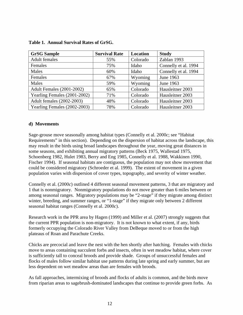
Rossi, CDOW, unpublished data). In northwest Colorado, 49% (n = 192/388) and 77% (n = 299/388) of females moved 2 and 4 miles from the lek of capture, respectively (Hausleitner 2003, A.D. Apa, CDOW, unpublished data). Nests are typically shallow bowls lined with leaves, feathers and small twigs placed on the ground at the base of a live sagebrush bush (Schroeder et al. 1999). GrSG clutch size ranges from 6-10 eggs, with 7-9 being the most common (Griner 1939, Wallestad and Pyrah 1974, Connelly et al. 1993, Gregg et al. 1994, Schroeder 1997). In Moffat County, Colorado, GrSG clutch size averaged 5.7 eggs for yearling females and 7.0 eggs for adult females (overall average was 6.7 eggs; Hausleitner 2003). In addition, Peterson (1980) reported that the clutch of adult females was 7.0 eggs (range 6-9) and yearling clutches averaged 6.7 eggs (range 5-9). Incubation does not start until the last egg is laid and eggs are incubated 27 to 28 days (Patterson 1952, Peterson 1980). GrSG have one of the lowest nest success rates of all the upland game bird species (Schroeder 1997), ranging from 63% in Montana to 10% in Oregon (Drut 1994, Connelly et al. 2000c). In Moffat County, nest success in 2001-02 ranged from 45-60% (Hausleitner 2003). GrSG nest abandonment is not uncommon if the hen is disturbed. While re-nesting is infrequent, it does occur (Patterson 1952, Eng 1963, Hulet 1983, Connelly et al. 1991). Peterson (1980) reported a 33.3% re-nesting rate (females that lost their first nest and attempted to re-nest), while Hausleitner (2003) reported lower re-nesting rates of 8 and 15% in 2001 and 2002, respectively. Clutch size of re-nesting attempts varies from 4-7 eggs (Schroeder 1997). Although clutch initiation dates (date of first egg laid) can vary among years and locations, Hausleitner (2003) reported the mean clutch initiation date in Moffat County, Colorado as 26 April in 2001, and 21 April for 2002. Hatching begins around mid-May and usually ends by July. Most eggs hatch in June, with a peak between June 10 and June 20. c) Survival The survival rate of GrSG varies by year, sex, and age (Zablan 1993). Adult GrSG survival rates have been estimated from banding or radio telemetry studies (Table 1). There is evidence to suggest that adult female sage-grouse have higher survival rates than do adult males (Swenson 1986). This higher survival rate may be due to sexual dimorphism. Females have cryptic plumage and a more secretive nature, versus the more elaborate plumage and display activities of males (Schroeder et al. 1999). Seasonal female survival in Colorado was highest in winter (Hausleitner 2003). Predation, both on eggs and birds, appears to be a primary cause of mortality (Schroeder et al. 1999); human predation through sport harvest is also a cause of mortality. The availability of food and cover are key factors related to chick and juvenile survival. In Wyoming, survival of juveniles from hatch to fall was estimated to be 38% (June 1963).

12

Table 1. Annual Survival Rates of GrSG. GrSG Sample Survival Rate Location Study Adult females 55% Colorado Zablan 1993 Females 75% Idaho Connelly et al. 1994 Males 60% Idaho Connelly et al. 1994 Females 67% Wyoming June 1963 Males 59% Wyoming June 1963 Adult Females (2001-2002) 65% Colorado Hausleitner 2003 Yearling Females (2001-2002) 71% Colorado Hausleitner 2003 Adult females (2002-2003) 48% Colorado Hausleitner 2003 Yearling Females (2002-2003) 78% Colorado Hausleitner 2003

d) Movements Sage-grouse move seasonally among habitat types (Connelly et al. 2000c; see “Habitat Requirements” in this section). Depending on the dispersion of habitat across the landscape, this may result in the birds using broad landscapes throughout the year, moving great distances in some seasons, and exhibiting annual migratory patterns (Beck 1975, Wallestad 1975, Schoenberg 1982, Hulet 1983, Berry and Eng 1985, Connelly et al. 1988, Wakkinen 1990, Fischer 1994). If seasonal habitats are contiguous, the population may not show movement that could be considered migratory (Schroeder et al. 1999). The extent of movement in a given population varies with dispersion of cover types, topography, and severity of winter weather. Connelly et al. (2000c) outlined 4 different seasonal movement patterns, 3 that are migratory and 1 that is nonmigratory. Nonmigratory populations do not move greater than 6 miles between or among seasonal ranges. Migratory populations may be “2-stage” if they migrate among distinct winter, breeding, and summer ranges, or “1-stage” if they migrate only between 2 different seasonal habitat ranges (Connelly et al. 2000c). Research work in the PPR area by Hagen (1999) and Miller et al. (2007) strongly suggests that the current PPR population is non-migratory. It is not known to what extent, if any, birds formerly occupying the Colorado River Valley from DeBeque moved to or from the high plateaus of Roan and Parachute Creeks. Chicks are precocial and leave the nest with the hen shortly after hatching. Females with chicks move to areas containing succulent forbs and insects, often in wet meadow habitat, where cover is sufficiently tall to conceal broods and provide shade. Groups of unsuccessful females and flocks of males follow similar habitat use patterns during late spring and early summer, but are less dependent on wet meadow areas than are females with broods. As fall approaches, intermixing of broods and flocks of adults is common, and the birds move from riparian areas to sagebrush-dominated landscapes that continue to provide green forbs. As

13

late fall approaches, weather events trigger movements to winter areas. The timing of this movement varies, influenced by yearly weather conditions. Very little is known about dispersal of GrSG juveniles following brood breakup. Dunn and Braun (1985) found that females moved farther than males between their natal area lek and the lek attended in the following spring. GrSG winter range in Colorado varies according to snowfall, wind conditions, and suitable habitat (Rogers 1964). Sage-grouse may travel short distances or many miles between seasonal ranges. Movements in fall and early winter (September-December) can be extensive, sometimes exceeding 20 miles. In North Park, Colorado, Schoenberg (1982) documented female GrSG moving more than 18 miles from winter to nesting areas. Hausleitner (2003) found that in Moffat County, Colorado, female GrSG moved an average of 6 miles from nesting areas to winter sites. The range of movements was extensive, and ranged from < 0.5-19 miles. Flock size in winter is variable (15-100+), with GrSG flocks frequently comprised of a single sex (Beck 1977). Many, but not all, flocks of GrSG males can over-winter in the vicinity of their leks, and by March they are usually within 2-3 miles of breeding areas used the previous year. These movements depend on whether the population is non-migratory or moves between 2 or more seasonal ranges (Connelly et al. 2000c). 4) Habitat Requirements Sage-grouse habitat requirements may differ by season (Connelly et al. 2000c). Connelly et al. (2000c) segregated habitat requirement into 4 seasons: (1) breeding habitat; (2) summer - late brood-rearing habitat; (3) fall habitat; and (4) winter habitat. In some situations, fall and summer-late brood-rearing habitats are indistinguishable, but this depends on the movement patterns of the population and habitat availability. The breeding habitat category includes lekking, pre-laying female, nesting, and early brood-rearing habitat. Summer-late brood-rearing habitat includes habitat used during this period by males, non-brooding females, and females with broods. Fall habitat consists of “transition” range from late summer to winter, and can include a variety of habitats used by males and females (with and without broods). Winter habitat is used by segregated flocks of males and females (Beck 1977). Management of sage-grouse habitats should include all habitat types necessary for fulfillment of life history needs. For the purpose of this Plan, we have combined the summer-late brood-rearing and fall habitat into a single habitat category, “summer-fall”, resulting in 3 overall seasonal habitats, rather than 4. Summer-late brood-rearing habitat in Colorado is typically characterized by high elevation mesic areas, cropland, wet meadows, and riparian areas adjacent to sagebrush communities. Grouse continue to use these locales as fall approaches and there is a slow conversion of the diet from forbs to sagebrush. As mentioned earlier, in many cases these 2 seasonal habitats are indistinguishable, but in the future, local information may provide additional insight as to when and where late-summer and fall habitats can be clearly separated. All the seasonal habitats described here include habitat used by brooding females, unsuccessful females, and male flocks.

14

a) Breeding Habitat: Leks (March – mid-May) Lek sites can be very traditional, with grouse displaying in the very same location from year to year. Some GrSG leks in Colorado are known to have been in use since the 1950’s (Rogers 1964). Leks are usually located in small, open areas, adjacent to stands of sagebrush with 20% or greater canopy cover (Klott and Lindzey 1989). Openings are usually natural, including alkali flats and meadows within sagebrush, but they may also be created by humans, including (but not limited to) small burns, drill pads, irrigated pasture, and roads within sagebrush habitat (Connelly et al. 1981, Gates 1985). Lek sites do not appear limiting (Schroeder et al. 1999), but they may vary in amount of escape cover and quality of sagebrush (Patterson 1952, Gill 1965, Connelly et al. 1988, Connelly et al. 2000c). The size of area needed for males to strut can vary greatly. Lek sites are usually flat to gently sloping areas of <15% slope in broad valleys or on ridges (Hanna 1936, Patterson 1952, Hartzler 1972, Giezentanner and Clark 1974, Wallestad 1975, Dingman 1980, Autenrieth 1981, Klott and Lindzey 1989). Lek sites have good visibility and low vegetation structure (Tate et al. 1979, Connelly et al. 1981, Gates 1985), and acoustical qualities that allow sounds of breeding displays to carry (Patterson 1952, Hjorth 1970, Hartzler 1972, Wiley 1973b, 1974, Bergerud 1988a, Phillips 1990). The absence of tall shrubs, trees, or other obstructions appears to be critical for continued use of these sites by displaying males. Sites chosen for display are typically close to sagebrush that is > 6 inches tall and has a canopy cover > 20% (Wallestad and Schladweiler 1974). Usually leks are located in the vicinity of nesting habitat (Wakkinen et al. 1992), and are in areas intersected by high female GrSG traffic (Bradbury and Gibson 1983, Bradbury et al. 1986, Gibson et al. 1990, Gibson 1992, 1996). These sagebrush areas are used for feeding, roosting, and escape from inclement weather and predators. Males are usually found roosting in sagebrush stands with canopy cover of 20-30% (Wallestad and Schladweiler 1974). Daytime movements of adult male GrSG during the breeding season do not vary greatly. Wallestad and Schladweiler (1974) found daily movements ranged between 0.2 and 0.8 miles from leks, with a maximum cruising radius of 0.9 to 1.2 miles. Ellis et al. (1987) reported that dispersal flights of male GrSG (to day-use areas) ranged from 0.3 – 0.5 miles, with the longest flights ranging from 1.2 – 1.3 miles. Carr (1967) recorded a cruising radius for male GrSG that ranged from 0.9-1.1 miles. Rothenmaier (1979) found that 60-80% of male GrSG locations were within 0.6-0.7 miles of a lek. Emmons (1980) reported that male dispersal distances to day-use areas of 0.1 miles were common and that 67% of all use areas were greater than 0.3 miles from the lek. In addition, Schoenberg (1982) found that male daily movements averaged 0.6 miles, but ranged from 0.02-1.5 miles. b) Breeding Habitat: Pre-laying (late-March – April) Connelly et al. (2000c) recommend that breeding habitat should be defined to include pre-laying habitat, but little is known or understood about pre-laying habitat. It has been suggested that pre-laying sagebrush habitat should provide a diversity of understory vegetation to meet the nutritional needs of females during the egg development period. For pre-laying females in

15

Oregon, Barnett and Crawford (1994) suggested that the habitat should contain a diversity of forbs that are rich in calcium, phosphorous, and protein. c) Breeding Habitat: Nesting (mid-April – June) GrSG prefer to nest under tall (11-31 inches) sagebrush (Connelly et al. 2000c). Peterson (1980) found in North Park, Colorado that nest shrubs averaged approximately 20 inches. In Moffat County, Colorado, this value is slightly higher and ranges from 30-32 inches (Hausleitner 2003). Often, the actual nest bush is taller than the surrounding sagebrush plants (Keister and Willis 1986, Wakkinen 1990, Apa 1998). In northwestern Colorado, the nest bush was nearly 10 inches taller than surrounding shrubs (Hausleitner 2003). The canopy cover of sagebrush around the nest ranges from 15-38% (Patterson 1952, Gill 1965, Gray 1967, Wallestad and Pyrah 1974, Keister and Willis 1986, Wakkinen 1990, Connelly et al. 1991, Apa 1998, Connelly et al. 2000c). Sagebrush canopy cover around nests in northwestern Colorado had a similar range of values, and averaged 27% (Hausleitner 2003). Good quality nesting habitat consists of live sagebrush with sufficient canopy cover, and substantial grasses and forbs in the understory (Connelly et al. 2000c, Hausleitner et al. 2005). Few herbaceous plants are growing in April when nesting begins, so residual herbaceous cover from the previous growing season is critical for nest concealment in most areas, although the level of herbaceous cover depends largely on the potential of the sagebrush community (Connelly et al. 2000c). Nearly all nests are located beneath sagebrush plants (Patterson 1952, Gill 1965, Gray 1967, Wallestad and Pyrah 1974), and GrSG nesting under sagebrush plants have higher nest success than those that nest under plants other than sagebrush (Connelly et al. 1991). Herbaceous vegetation is also important in sage-grouse nest sites (Connelly et al. 2000c). Grass heights are variable and, as measured across the West, range from 5-13 inches (Connelly et al. 2000c). In addition, horizontal grass cover measurements are also variable and range from 4-51% cover. These measurements are similar to data from northwestern Colorado; Hausleitner (2003) reported that grass heights at nests ranged from 5-6 inches, grass cover averaged approximately 4%, and forb cover averaged about 7% (Hausleitner 2003). Although not clearly understood, it is also believed that understory herbaceous cover (horizontal and vertical) is important for GrSG nesting habitat. In multiple studies, nest sites had taller and more grass cover, and less bare ground, than did random sites (Klebenow 1969, Wakkinen 1990, Sveum et al. 1998b, Holloran 1999, Lyon 2000, Slater 2003). In Oregon, both forb and tall grass cover appeared related to nest initiation, re-nesting, and nest success rates (Coggins 1998). d) Breeding Habitat: Early Brood-Rearing (mid-May – July) Early brood-rearing habitat requirements are very similar to those for nesting habitat. Early brood-rearing habitat is found relatively close to nest sites (Connelly et al. 2000c), but individual females with broods may move large distances (Connelly 1982, Gates 1983). Early brood-rearing habitat is typically characterized by sagebrush stands with canopy cover of 10-15% (Martin 1970, Wallestad 1971), and with understories that exceed 15% herbaceous cover (Sveum

16

et al. 1998a, Lyon 2000). In Moffat County, Colorado, sagebrush stands averaged approximately 11% canopy cover, and herbaceous understories averaged about 14% horizontal cover (Hausleitner 2003). High plant species diversity (sometimes also referred to as species richness) is also typical in early brood-rearing habitat (Dunn and Braun 1986, Klott and Lindzey 1990, Drut et al. 1994a, Apa 1998). Sagebrush heights ranged from 6-18 inches in Washington and Wyoming (Sveum et al. 1998a, Lyon 2000), and averaged about 23 inches in Moffat County (Hausleitner 2003). Adjacent shrub areas of 20-25% canopy cover have been reported as preferred for escape and day roosting (Wallestad 1971, Dunn and Braun 1986), but night roosting sites in Moffat County, Colorado had only 4% sagebrush canopy cover and sagebrush height was 20 inches (Hausleitner 2003). In early summer, the size of the area used by GrSG appears to depend on the interspersion of sagebrush types that provide an adequate amount of food and cover. Females and broods may select riparian habitats in the sagebrush type that have abundant forbs and moisture (Gill 1965, Klebenow 1969, Savage 1969, Connelly and Markham 1983, Gates 1983, Connelly et al. 1988, Fischer et al. 1996a). Females with broods remain in sagebrush uplands as long as the vegetation remains succulent, but may move to wet meadows as vegetation desiccates (Fischer et al. 1996b). Depending on precipitation and topography, some broods may stay in sagebrush/grass communities all summer while others shift to lower areas (riparian areas, hay meadows or alfalfa fields) as upland plant communities desiccate (Wallestad 1975). For the PPR, broods are generally not found in the alfalfa fields, hay meadows, or riparian areas in the lower valleys and canyons; they probably use mesic upland sites and headwater riparian areas. Local rancher Tim Uphoff can recall only a few instances over four decades that he’s seen birds along the West Fork of Parachute Creek. e) Summer - Fall Habitat (July – September) As sagebrush communities continue to dry out and many forbs complete their life cycles, sage-grouse typically respond by moving to a greater variety of habitats, and generally more mesic habitats (Patterson 1952). Sage-grouse begin movements in late June and into early July (Gill 1965, Klebenow 1969, Savage 1969, Connelly and Markham 1983, Gates 1983, Connelly et al. 1988, Fischer 1994). By late summer and into the early fall, females with broods, non-brood females, and groups of males become more social, and flocks are more concentrated (Patterson 1952). This is the period of time when GrSG can be observed in atypical habitat such as farmland and irrigated habitats (Connelly and Markham 1983, Gates 1983, Connelly et al. 1988). From mid-September into October, GrSG prefer areas with more dense sagebrush (>15% canopy cover) and late green succulent forbs before moving to early transitional winter range where sexual segregation of flocks becomes notable (Wallestad 1975, Beck 1977, Connelly et al. 1988). During periods of heavy snow cover in late fall and early winter, use of mountain and Wyoming big sagebrush stands is extensive.

17

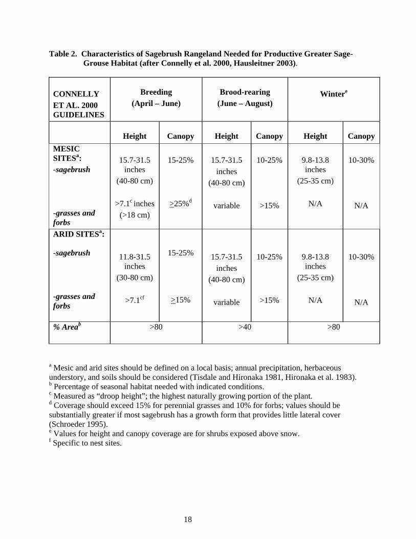
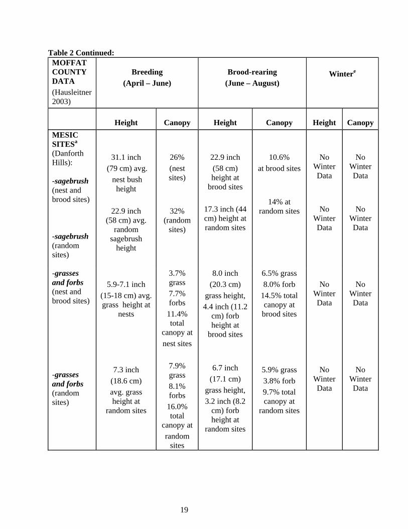
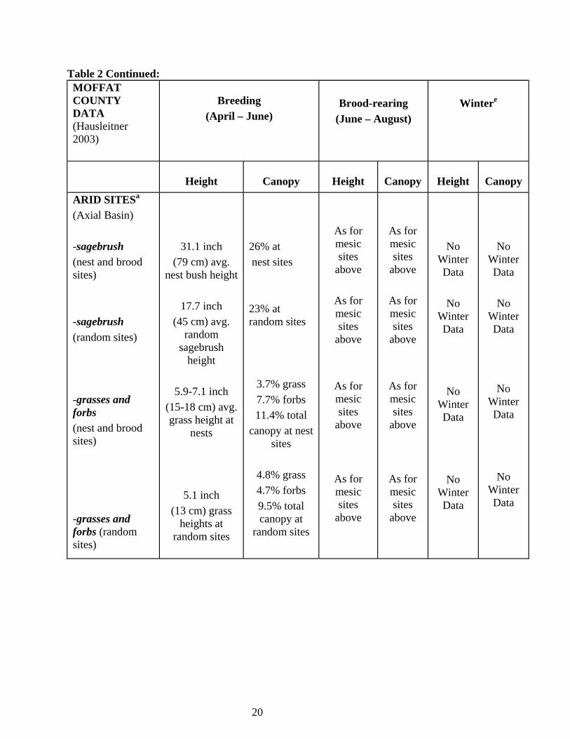
f) Winter Habitat (October-February) GrSG winter habitat use depends upon snow depth and availability of sagebrush, which is used almost exclusively for both food and cover. Used sites are typically characterized by canopy cover >25% and sagebrush >12-16 inches tall (Schoenberg 1982), and are associated with drainages, ridges, or southwest aspects with slopes < 15% (Gill 1965, Wallestad 1975, Beck 1977, Robertson 1991). In Colorado, <10% of sagebrush habitat is used by GrSG during deep snow conditions (Beck 1977) because most of the sagebrush is buried under the snow. When snow deeper than 12 inches covers over 80% of the winter range, GrSG in Idaho have been shown to rely on sagebrush greater than 16 inches in height for foraging (Robertson 1991). Doherty et al. (2008) found that females preferred landscapes with extensive sagebrush habitat and gentle to flat terrain, and avoided areas with conifers, woody riparian zones, and rough terrain. Lower flat areas and shorter sagebrush along ridge tops provide roosting and feeding areas. During extreme winter conditions, GrSG will spend nights and portions of the day (when not foraging) burrowed into “snow roosts” (Back et al. 1987). When snow has the proper texture, snow roosts are dug by wing movements or by scratching with the feet. Hupp and Braun (1989b) found that most GuSG feeding activity during the winter occurred in drainages and on slopes with south or west aspects in the Gunnison Basin. In years with severe winters resulting in heavy accumulations of snow, the amount of sagebrush exposed above the snow can be severely limited. Hupp and Braun (1989b) investigated GuSG feeding activity during a severe winter in the Gunnison Basin in 1984, where they estimated <10% of the sagebrush was exposed above the snow and available to sage-grouse. In these conditions, the tall and vigorous sagebrush typical in drainages were an especially important food source for GuSG. Although no specific research has been conducted on winter habitat characteristics or food habitats of Greater Sage-Grouse in the Parachute-Piceance-Roan area, information collected in other parts of Colorado and throughout their range can be used to predict habitat use and food requirements in this area. Connelly et al. (2000) summarizes the characteristics of productive sagebrush habitat for average western sites used by Greater Sage-Grouse in Table 2. Hausleitner (2003) has more specific information for Moffat County, Colorado breeding and brood-rearing habitat. Some of the vegetation values are higher in Moffat Co. than rest of the U.S., which may also be the case for Rio Blanco and Garfield Counties.

18

Table 2. Characteristics of Sagebrush Rangeland Needed for Productive Greater Sage-Grouse Habitat (after Connelly et al. 2000, Hausleitner 2003).

CONNELLY ET AL. 2000 GUIDELINES

Breeding

(April – June)

Brood-rearing

(June – August)

Wintere

Height

Canopy

Height

Canopy

Height

Canopy

MESIC SITESa: -sagebrush -grasses and forbs

15.7-31.5

inches (40-80 cm)

>7.1c inches

(>18 cm)

15-25%

>25%d

15.7-31.5

inches (40-80 cm)

variable

10-25%

>15%

9.8-13.8 inches

(25-35 cm)

N/A

10-30%

N/A

ARID SITESa: -sagebrush

-grasses and forbs

11.8-31.5 inches

(30-80 cm)

>7.1cf

15-25%

>15%

15.7-31.5 inches

(40-80 cm)

variable

10-25%

>15%

9.8-13.8 inches

(25-35 cm)

N/A

10-30%

N/A

% Areab

>80 >40 >80

a Mesic and arid sites should be defined on a local basis; annual precipitation, herbaceous understory, and soils should be considered (Tisdale and Hironaka 1981, Hironaka et al. 1983). b Percentage of seasonal habitat needed with indicated conditions. c Measured as “droop height”; the highest naturally growing portion of the plant. d Coverage should exceed 15% for perennial grasses and 10% for forbs; values should be substantially greater if most sagebrush has a growth form that provides little lateral cover (Schroeder 1995). e Values for height and canopy coverage are for shrubs exposed above snow. f Specific to nest sites.

19

Table 2 Continued: MOFFAT COUNTY DATA (Hausleitner 2003)

Breeding

(April – June)

Brood-rearing

(June – August)

Wintere

Height

Canopy

Height

Canopy

Height

Canopy

MESIC SITESa

(Danforth Hills): -sagebrush (nest and brood sites) -sagebrush (random sites)

31.1 inch (79 cm) avg.

nest bush height

22.9 inch

(58 cm) avg. random

sagebrush height

26% (nest sites)

32% (random

sites)

22.9 inch (58 cm) height at

brood sites

17.3 inch (44 cm) height at random sites

10.6% at brood sites

14% at random sites

No Winter Data

No Winter Data

No Winter Data

No Winter Data

-grasses and forbs (nest and brood sites) -grasses and forbs (random sites)

5.9-7.1 inch

(15-18 cm) avg. grass height at

nests

7.3 inch (18.6 cm) avg. grass height at

random sites

3.7% grass 7.7% forbs

11.4% total

canopy at nest sites

7.9% grass 8.1% forbs

16.0% total

canopy at random

sites

8.0 inch (20.3 cm)

grass height, 4.4 inch (11.2

cm) forb height at

brood sites

6.7 inch (17.1 cm)

grass height, 3.2 inch (8.2

cm) forb height at

random sites

6.5% grass 8.0% forb

14.5% total canopy at brood sites

5.9% grass 3.8% forb 9.7% total canopy at

random sites

No

Winter Data

No Winter Data

No

Winter Data

No Winter Data

20

Table 2 Continued: MOFFAT COUNTY DATA (Hausleitner 2003)

Breeding

(April – June)

Brood-rearing

(June – August)

Wintere

Height

Canopy

Height

Canopy

Height

Canopy

ARID SITESa (Axial Basin) -sagebrush (nest and brood sites) -sagebrush (random sites) -grasses and forbs (nest and brood sites) -grasses and forbs (random sites)

31.1 inch (79 cm) avg.

nest bush height

17.7 inch (45 cm) avg.

random sagebrush

height

5.9-7.1 inch (15-18 cm) avg. grass height at

nests

5.1 inch (13 cm) grass

heights at random sites

26% at nest sites 23% at random sites

3.7% grass 7.7% forbs 11.4% total

canopy at nest sites

4.8% grass 4.7% forbs 9.5% total canopy at

random sites

As for mesic sites

above

As for mesic sites

above

As for mesic sites

above

As for mesic sites

above

As for mesic sites

above

As for mesic sites

above

As for mesic sites

above

As for mesic sites

above

No Winter Data

No

Winter Data

No Winter Data

No Winter Data

No Winter Data

No

Winter Data

No Winter Data

No Winter Data

21

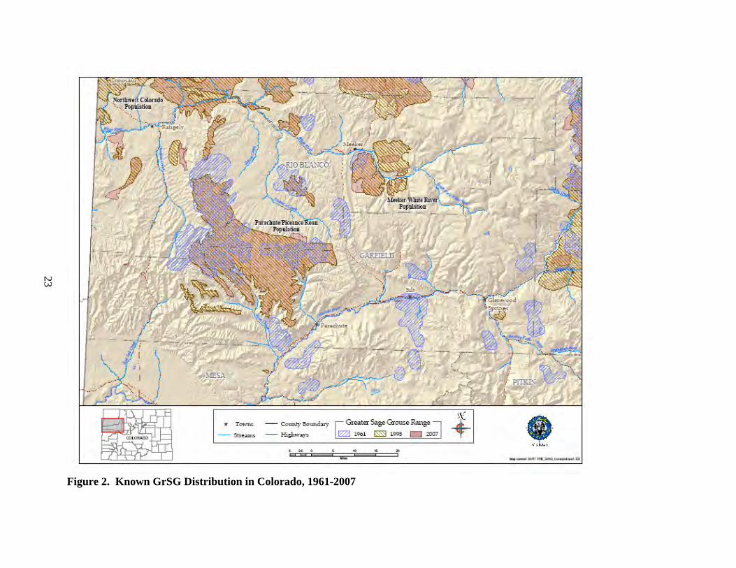
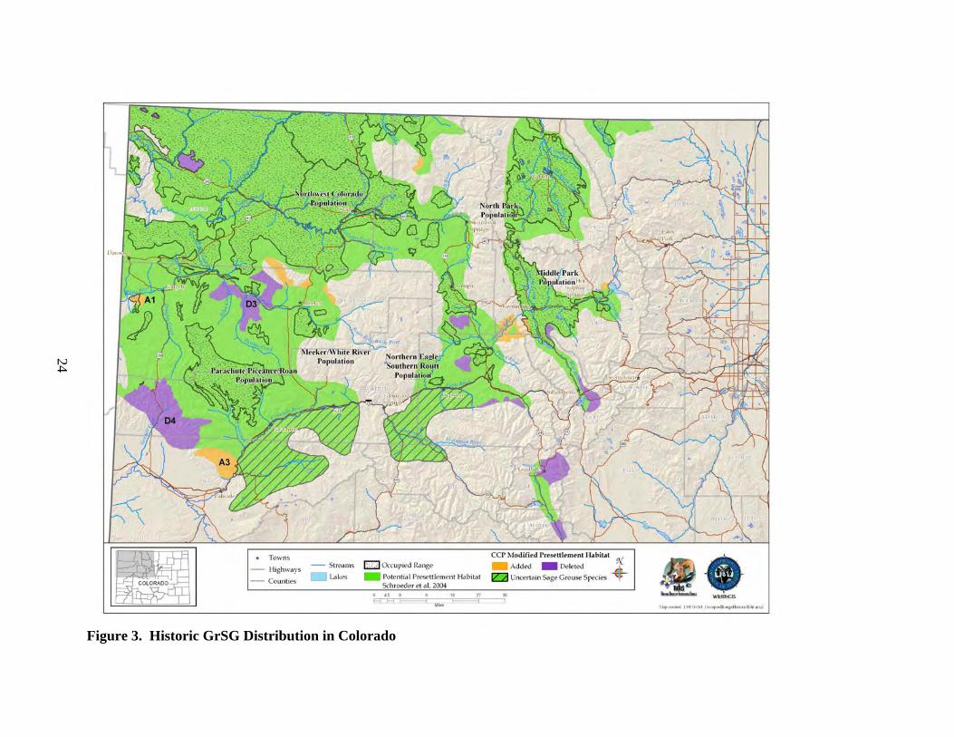
B. Distribution and Abundance 1) Distribution a) Historic Distribution The historic distribution of GrSG is closely tied to and largely reflects the distribution of sagebrush, particularly big sagebrush, and to some extent, silver sagebrush (Braun 1995, Schroeder et al. 2004). Direct observations and specimens of GrSG prior to the 1900s are limited in number and may not be adequate for drawing a historical distribution map. Instead, a map of historic sagebrush distribution can provide a reasonable and more thorough approximation of GrSG distribution. Beginning in 1957, CDOW’s Glenn Rogers began to gather and update information on sage-grouse distribution in Colorado. One of his objectives was to determine the historic and current distribution of the species in the state. He conducted interviews of CDOW field personnel and landowners, flew fixed-wing aircraft searches, and counted known strutting grounds (leks). From his five-year effort, Rogers (1964) drew a map that estimated the historic sage-grouse range in Colorado (Fig. 2). In the PPR area, the map shows occupied areas west to the Utah line, on both sides of the Colorado River from roughly Silt to DeBeque, on both sides of Colorado State Highway (CSH) 13 from Rifle to Meeker, and south of Rifle. Braun (1995) repeated the process in the early 1990’s, using a literature review, interviews and field work to determine sage-grouse occupied range. He reported his findings by county and provided a map of the birds’ distribution at that point in time. He estimated that “both distribution and abundance of sage-grouse in Colorado have decreased more that 50% since the early 1900’s”. Figure 2 also shows Braun’s 1995 map over the historic distribution reported by Rogers (1964). Schroeder et al. (2004) presented a “pre-settlement” map (Fig. 3) of sagebrush habitat, targeting a period before pioneers of European descent inhabited the area. The map is based on a vegetation map by Kuchler (1985) and 7 GrSG “core” habitat types identified by Schroeder et al. (2004). Some of these “core” habitats are considered grasslands (of various plant species), but only local portions of these habitats known to be dominated by sagebrush were included in the pre-settlement map (Schroeder et al. 2004). In addition, 6 “secondary” habitat types, which may be of importance to GrSG under certain conditions, were included in the map if they were in currently or previously known occupied habitat, or if they were within 6 miles of core habitat (Schroeder et al. 2004). The vegetation data layer used by Schroeder was adequate for depicting rough historic range, but many inaccuracies became apparent at a statewide level with more robust vegetation datasets for comparison. In Colorado, sagebrush was historically distributed in a discontinuous pattern, interrupted by topography and forested habitat (Braun 1995). GrSG occupied some portion of 13 counties in Colorado (Braun 1995, Schroeder et al. 2004). The Colorado portion of the historical map by Schroeder et al. (2004) was adjusted based on finer scale knowledge of local topography and the current distribution of habitat. Specifically, we used data from the Colorado Vegetation

22

Classification Project (CVCP, Colorado Division of Wildlife 2004b), a geographic information system (GIS) data set that uses recent satellite imagery and field verification to classify vegetation into specific categories. What appear to be minor differences in mapping at the rangewide scale have more significance at the statewide scale, so a more precise data set is valuable. Several small additions were made to the Colorado portion of the historic distribution map in Schroeder et al. (2004), where sagebrush currently occurs in the CVCP (Colorado Division of Wildlife 2004b), and where no evidence exists that vegetation other than sagebrush was historically present (Fig. 3). A few areas that are very small even at the state scale were added, but are not identified in the figure or table. Some areas, known to have no historical sagebrush occurrence, were also deleted from the map.

23

Figure 2. Known GrSG Distribution in Colorado, 1961-2007

24

Figure 3. Historic GrSG Distribution in Colorado

25

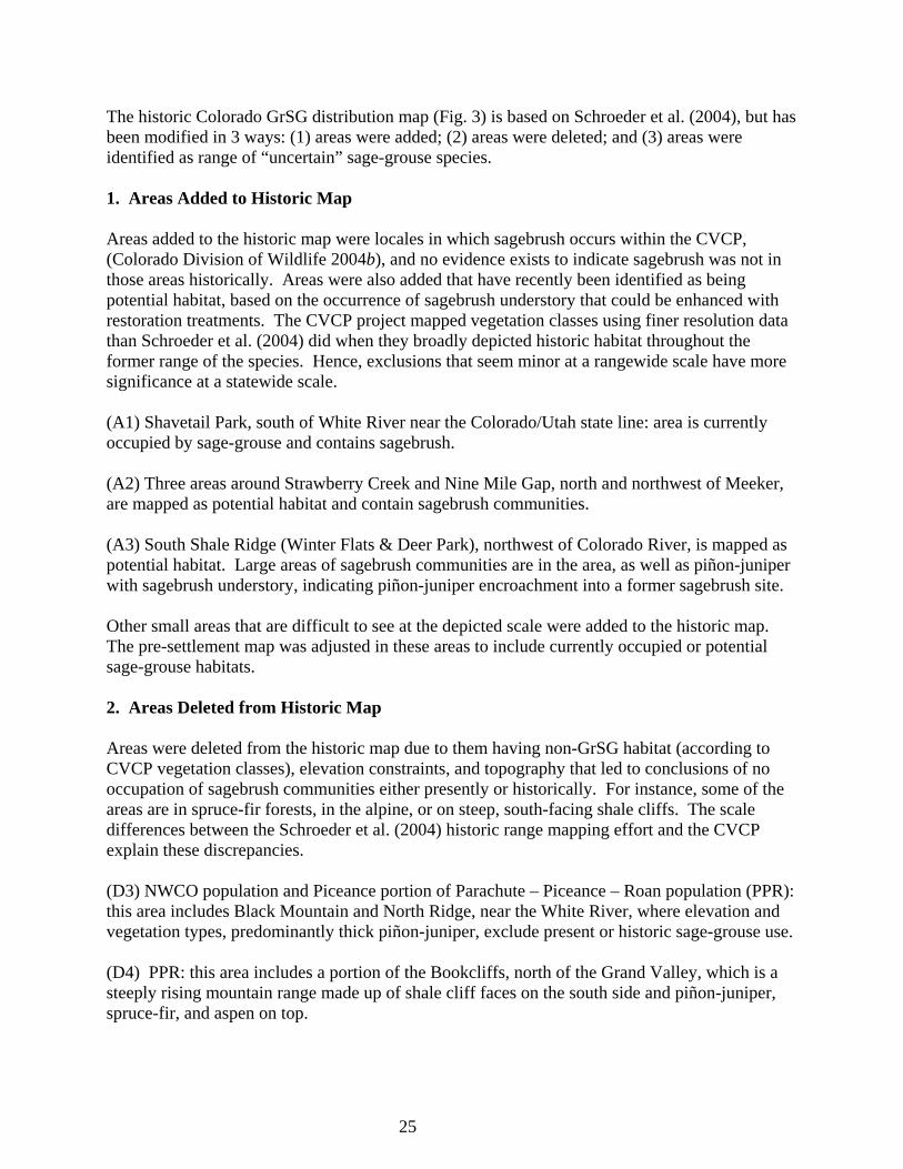
The historic Colorado GrSG distribution map (Fig. 3) is based on Schroeder et al. (2004), but has been modified in 3 ways: (1) areas were added; (2) areas were deleted; and (3) areas were identified as range of “uncertain” sage-grouse species. 1. Areas Added to Historic Map Areas added to the historic map were locales in which sagebrush occurs within the CVCP, (Colorado Division of Wildlife 2004b), and no evidence exists to indicate sagebrush was not in those areas historically. Areas were also added that have recently been identified as being potential habitat, based on the occurrence of sagebrush understory that could be enhanced with restoration treatments. The CVCP project mapped vegetation classes using finer resolution data than Schroeder et al. (2004) did when they broadly depicted historic habitat throughout the former range of the species. Hence, exclusions that seem minor at a rangewide scale have more significance at a statewide scale. (A1) Shavetail Park, south of White River near the Colorado/Utah state line: area is currently occupied by sage-grouse and contains sagebrush. (A2) Three areas around Strawberry Creek and Nine Mile Gap, north and northwest of Meeker, are mapped as potential habitat and contain sagebrush communities. (A3) South Shale Ridge (Winter Flats & Deer Park), northwest of Colorado River, is mapped as potential habitat. Large areas of sagebrush communities are in the area, as well as piñon-juniper with sagebrush understory, indicating piñon-juniper encroachment into a former sagebrush site. Other small areas that are difficult to see at the depicted scale were added to the historic map. The pre-settlement map was adjusted in these areas to include currently occupied or potential sage-grouse habitats. 2. Areas Deleted from Historic Map Areas were deleted from the historic map due to them having non-GrSG habitat (according to CVCP vegetation classes), elevation constraints, and topography that led to conclusions of no occupation of sagebrush communities either presently or historically. For instance, some of the areas are in spruce-fir forests, in the alpine, or on steep, south-facing shale cliffs. The scale differences between the Schroeder et al. (2004) historic range mapping effort and the CVCP explain these discrepancies. (D3) NWCO population and Piceance portion of Parachute – Piceance – Roan population (PPR): this area includes Black Mountain and North Ridge, near the White River, where elevation and vegetation types, predominantly thick piñon-juniper, exclude present or historic sage-grouse use. (D4) PPR: this area includes a portion of the Bookcliffs, north of the Grand Valley, which is a steeply rising mountain range made up of shale cliff faces on the south side and piñon-juniper, spruce-fir, and aspen on top.

26

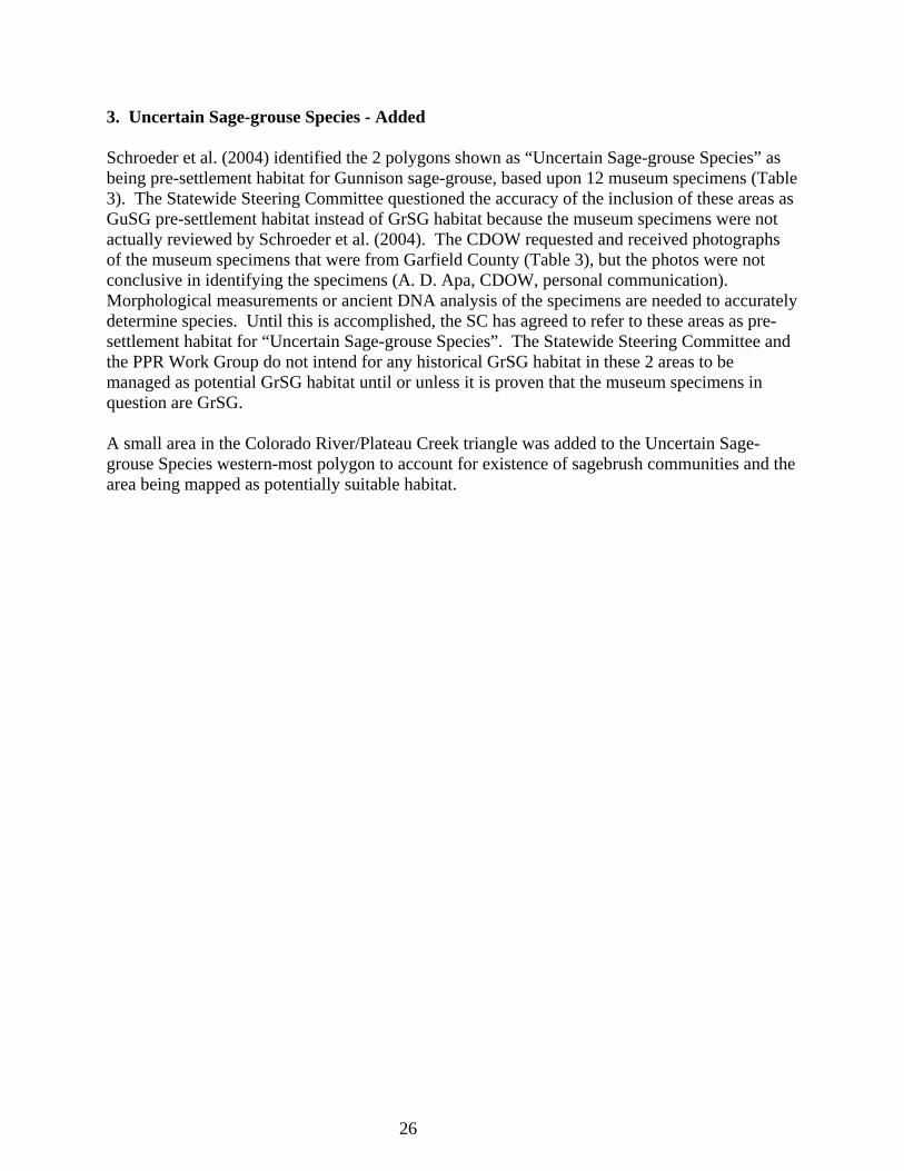
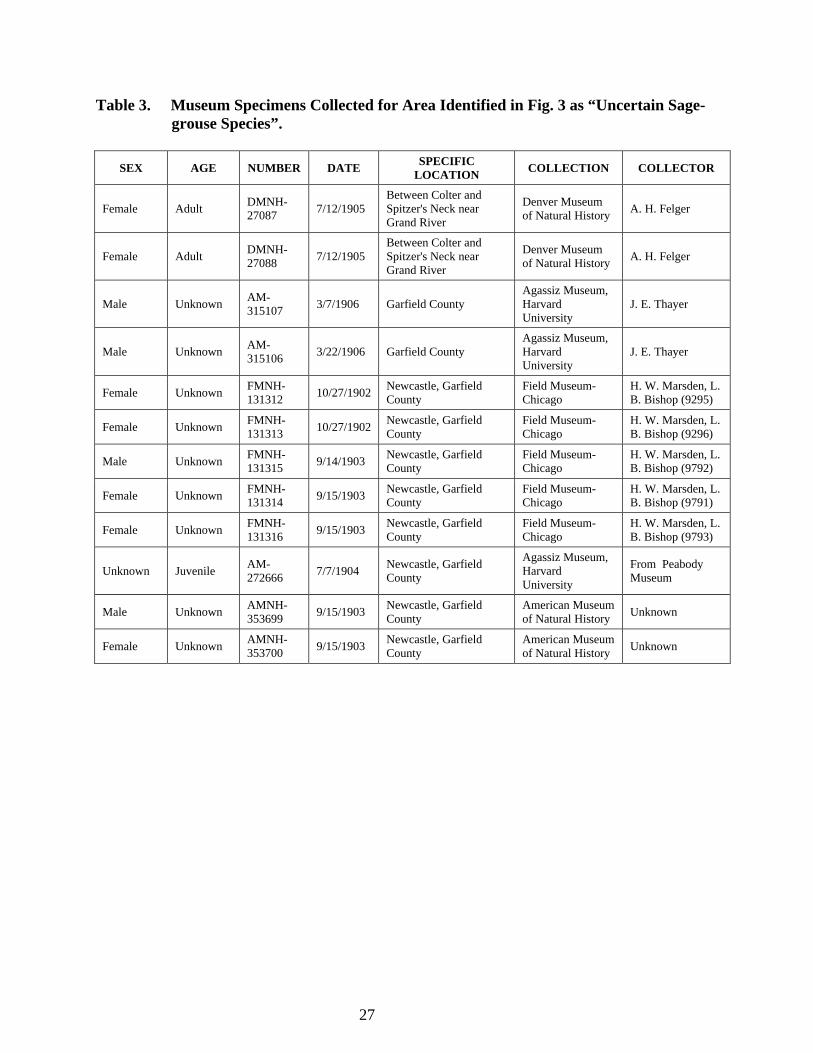
3. Uncertain Sage-grouse Species - Added Schroeder et al. (2004) identified the 2 polygons shown as “Uncertain Sage-grouse Species” as being pre-settlement habitat for Gunnison sage-grouse, based upon 12 museum specimens (Table 3). The Statewide Steering Committee questioned the accuracy of the inclusion of these areas as GuSG pre-settlement habitat instead of GrSG habitat because the museum specimens were not actually reviewed by Schroeder et al. (2004). The CDOW requested and received photographs of the museum specimens that were from Garfield County (Table 3), but the photos were not conclusive in identifying the specimens (A. D. Apa, CDOW, personal communication). Morphological measurements or ancient DNA analysis of the specimens are needed to accurately determine species. Until this is accomplished, the SC has agreed to refer to these areas as pre-settlement habitat for “Uncertain Sage-grouse Species”. The Statewide Steering Committee and the PPR Work Group do not intend for any historical GrSG habitat in these 2 areas to be managed as potential GrSG habitat until or unless it is proven that the museum specimens in question are GrSG. A small area in the Colorado River/Plateau Creek triangle was added to the Uncertain Sage-grouse Species western-most polygon to account for existence of sagebrush communities and the area being mapped as potentially suitable habitat.

27

Table 3. Museum Specimens Collected for Area Identified in Fig. 3 as “Uncertain Sage- grouse Species”.

SEX AGE NUMBER DATE SPECIFIC

LOCATION COLLECTION COLLECTOR

Female Adult DMNH-27087 7/12/1905

Between Colter and Spitzer's Neck near Grand River

Denver Museum of Natural History A. H. Felger

Female Adult DMNH-27088 7/12/1905

Between Colter and Spitzer's Neck near Grand River

Denver Museum of Natural History A. H. Felger

Male Unknown AM-315107 3/7/1906 Garfield County

Agassiz Museum, Harvard University

J. E. Thayer

Male Unknown AM-315106 3/22/1906 Garfield County

Agassiz Museum, Harvard University

J. E. Thayer

Female Unknown FMNH-131312 10/27/1902 Newcastle, Garfield

County Field Museum-Chicago

H. W. Marsden, L. B. Bishop (9295)

Female Unknown FMNH-131313 10/27/1902 Newcastle, Garfield

County Field Museum-Chicago

H. W. Marsden, L. B. Bishop (9296)

Male Unknown FMNH-131315 9/14/1903 Newcastle, Garfield

County Field Museum-Chicago

H. W. Marsden, L. B. Bishop (9792)

Female Unknown FMNH-131314 9/15/1903 Newcastle, Garfield

County Field Museum-Chicago

H. W. Marsden, L. B. Bishop (9791)

Female Unknown FMNH-131316 9/15/1903 Newcastle, Garfield

County Field Museum-Chicago

H. W. Marsden, L. B. Bishop (9793)

Unknown Juvenile AM-272666 7/7/1904 Newcastle, Garfield

County

Agassiz Museum, Harvard University

From Peabody Museum

Male Unknown AMNH-353699 9/15/1903 Newcastle, Garfield

County American Museum of Natural History Unknown

Female Unknown AMNH-353700 9/15/1903 Newcastle, Garfield

County American Museum of Natural History Unknown

28

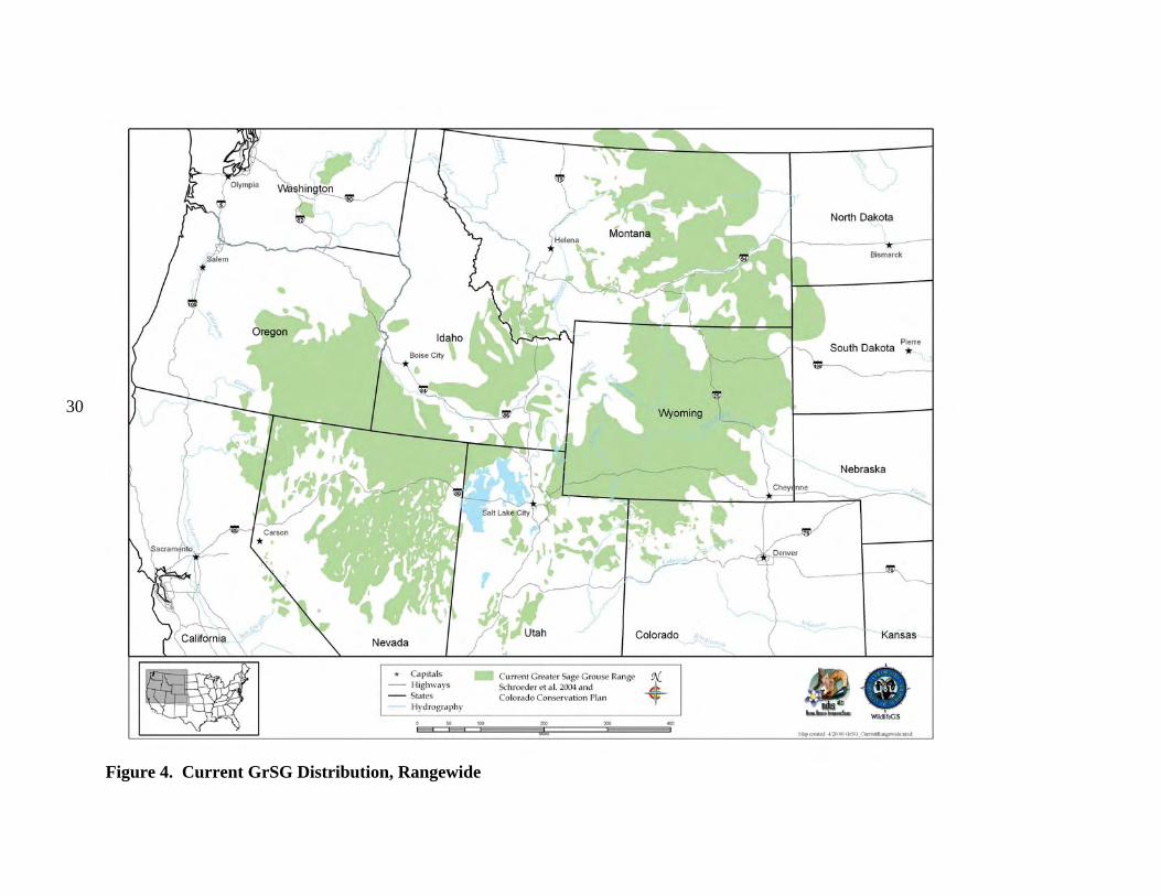
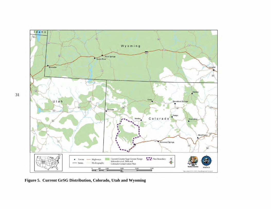
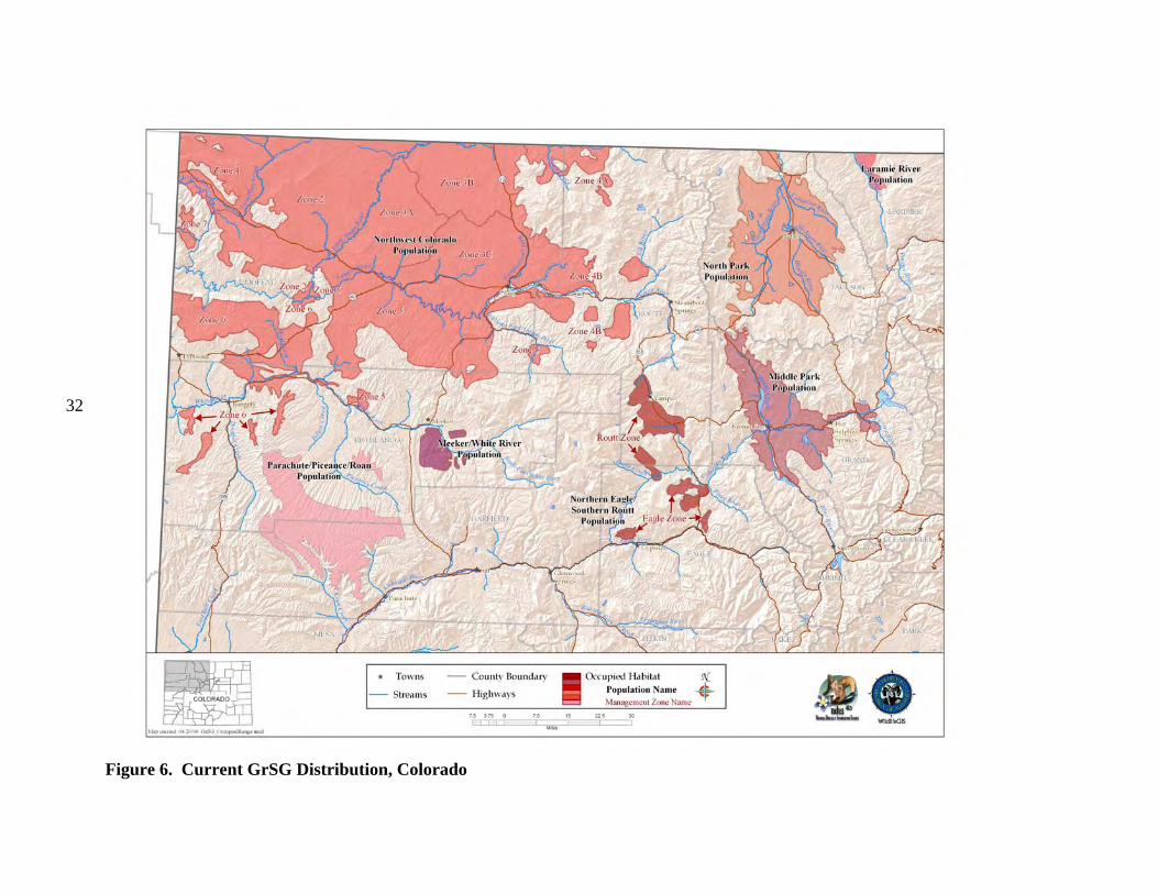
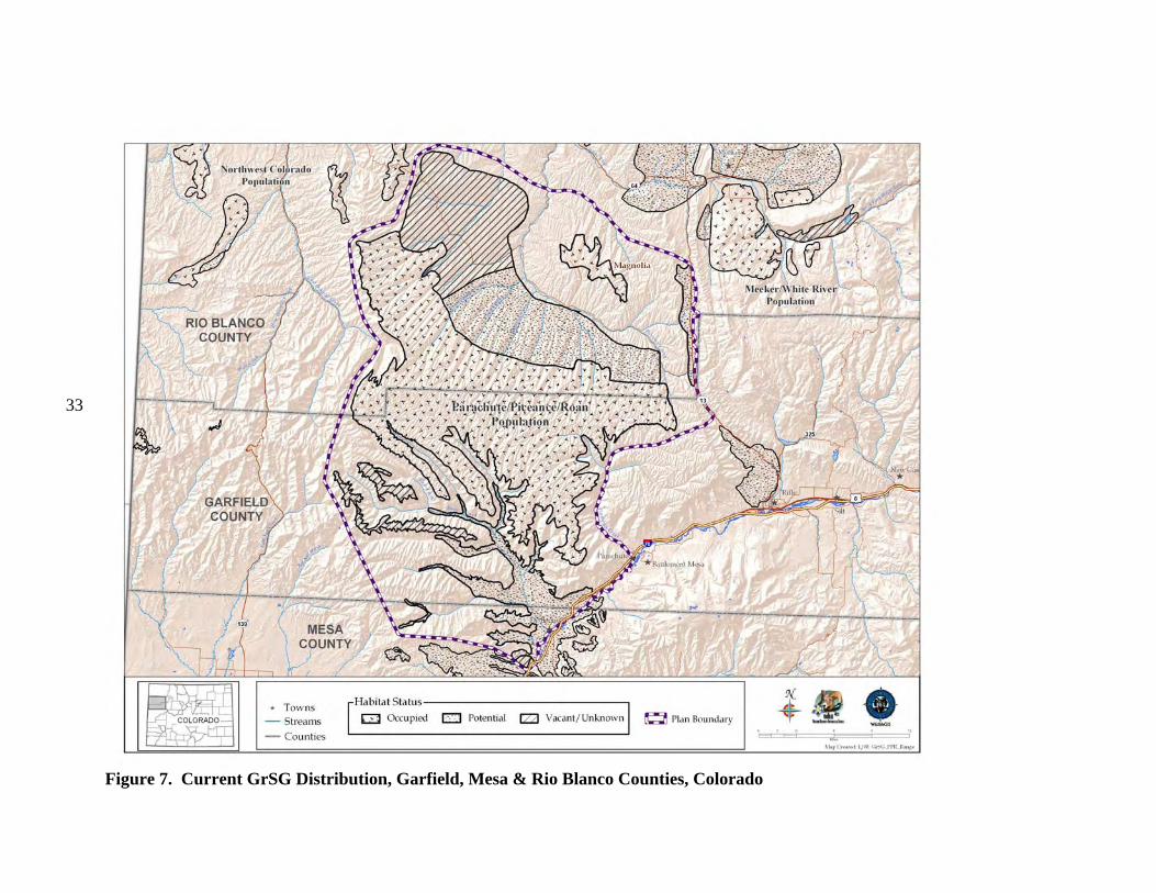
b) Current Distribution Colorado is on the southeastern edge of the current GrSG rangewide distribution (Fig. 4). It is, nevertheless, solidly within the range of the species, unlike some areas where populations were historically very limited in distribution and have since been extirpated (e.g., Nebraska; Fig. 4). Although GrSG distribution within Colorado has diminished (Braun 1995), the loss of range has been substantially less than in a number of other states, including Idaho, Oregon, and Washington. Thus, maintaining habitat and populations in Colorado will be important to conservation of GrSG on a rangewide basis. A closer view of the Colorado, Utah, and Wyoming region (Fig. 5) appears to indicate that some Colorado GrSG populations cross state borders. Radio telemetry research has confirmed that GrSG in NWCO are part of a tri-state population (A. D. Apa, CDOW, personal communication). Although this is not surprising, it does underscore the need for agencies to coordinate population and habitat management efforts among the 3 states. The current tri-state distribution map (Fig. 5) is based on Schroeder et al. (2004), except that current GrSG distribution in Colorado is based on a more detailed Colorado habitat mapping effort. Differences in map scale and data resolution between Schroeder et al. (2004) and the Colorado data are likely responsible for the apparent discontinuities in distribution that occur along state borders (Fig. 5). GrSG currently occur in 6 separate areas in the northwestern quarter of Colorado (Fig. 6; there is also a small group of birds that occur in the Laramie River Valley that are part of a larger Wyoming population). We term these areas “populations”, without implying that the populations are genetically distinct, or that they are completely isolated from each other. Rather, these “populations” are identified separately because they are, in most cases, physically separated to some degree, and individual local work groups have grown up around these separate GrSG areas to manage the “local” GrSG. Although many of the challenges facing GrSG are similar throughout the state, both biological and sociological issues may differ in importance among the different populations and local work groups. The populations occur in portions of 9 Colorado counties: Eagle, Garfield, Grand, Jackson, Larimer, Moffat, Rio Blanco, Routt, and Summit. The most abundant and widely distributed population is the Northwest Colorado (NWCO) population, centered in Moffat County (Fig. 6). In some populations, we have identified “zones”, or smaller areas within the population that are described separately and may be managed differently. In NWCO, the zones are based on GrSG management units used by the local Work Group. In the Northern Eagle – Southern Routt Counties population (NESR), 2 zones are described, based on the path of the Colorado River. The “Routt” zone lies north of the Colorado River and the “Eagle” zone lies south of the Colorado River. Note that this line of demarcation is close to, but not identical to the line between Eagle and Routt counties. A small numbers of GrSG occur in Larimer County (Laramie River population). The current overall range mapped by CDOW biologists and field personnel is also presented in Figure 7. It shows a further contraction in the range of the PPR population. The three maps provide a visual representation of the loss of overall range by the population during the 1900’s. Some of the early maps do not include much of the area we now include in the PPR population

29

area, likely due to the difficulty of getting around in that remote country during the soft snow and muddy spring conditions when grouse are most visible.

The primary range contraction has occurred on the southern end of the population. Assuming for this discussion that the grouse formerly found on both sides of the Colorado River were what are now known as Greater Sage-Grouse (there is not agreement on this in among sage-grouse experts; definitive proof one way or another is not known at the time of this writing), the range of what is now referred to in this Plan as the Parachute-Piceance-Roan population probably once extended below the Bookcliffs/Roan Plateau to the Rifle, Silt, Harvey Gap and Newcastle areas north of the river, and south of the river in Divide Creek, west to DeBeque, and across the “Sunnyside” area from DeBeque toward Collbran in the Plateau Creek Valley. Active leks were counted in the vicinity of Harvey Gap, north of Silt, and Hunter Mesa south of Rifle. Sage-grouse in these areas disappeared during the 1960’s, most likely due to loss of large expanses of sagebrush to agriculture (hay production and dryland farming). Grouse were present in the Plateau Valley more recently, but were gone by the 1980’s, with no one factor apparent as an obvious cause. On the western flanks of the former range, contraction has been more limited; three sage-grouse were seen on Kimball Mountain in the Roan Creek drainage in 1980; despite repeated observations over the years, primarily from fixed-wing aircraft, no GrSG were observed there again until June 2007, when 4 chicks were seen. To the north, one strutting grouse was seen on 4A Mountain in 1981, with no other sightings until 2006, when 2 males and one female were seen on one flight, and one female on a different flight that same spring. As recently as early 1989, sage-grouse were known in the low country west of DeBeque; three grouse were shot there by poachers who were subsequently apprehended by District Wildlife Manager Joe Gumber. Work Group member Chris Clark has a picture of 25-30 sage-grouse in winter on Colorado Highway 139 south of Rangely in winter during the mid-1990’s. These birds could have come from the Cathedral Bluffs area of the PPR population, or from the Zone 6 sub-population of the NW Colorado population (see Fig. 7).

On the north, “gaps” appear to have opened up between grouse considered to part of, or at least addressed in the context of, the Northwest Colorado Work Group, with some small areas south of the White River. The northern boundary of the PPR population is drawn at Yellow Creek and the birds in Zone 6 of the NW population occupy the upper reaches of the Duck Creeks near Calamity Ridge. Undoubtedly there is, or was historically, interchange between the two populations.

30

Figure 4. Current GrSG Distribution, Rangewide

31

Figure 5. Current GrSG Distribution, Colorado, Utah and Wyoming

32

Figure 6. Current GrSG Distribution, Colorado

33

Figure 7. Current GrSG Distribution, Garfield, Mesa & Rio Blanco Counties, Colorado

34

2) Abundance a) Lek Counts and Population Estimation Inventory and monitoring of wildlife populations is an obvious prerequisite to conserving them, and is especially important when quantitative goals for species conservation have been developed. What is not obvious is how to accomplish inventory, and what level of resources is appropriate to commit to this task, since resources devoted to inventory and monitoring will not be available for other critical conservation tasks. Having accurate and precise estimates of GrSG numbers does not in and of itself improve the species’ status. Population trends of sage-grouse have been monitored across the western U.S. using variations on a lek count methodology first described by Patterson (1952), who studied sage-grouse in Wyoming. Patterson speculated that the maximum number of males counted over 3 or 4 counts spread throughout the display period might be a useful index of sage-grouse population trends. Wildlife managers have monitored populations of many species through the use of indices, where a count or measurement is made of some characteristic of a population that is both convenient to measure and is thought to be related to abundance. With birds, indices are often based on vocalizations made during the breeding season, such as pheasant “crow” call counts, dove coo-count indices, and bobwhite whistling counts (Lancia et al. 1994). Anderson (2001) noted the weaknesses of this type of sampling, which may be convenient for wildlife managers, but does not lead to defensible estimates of population size or status. The index, whether it is pheasant crows or the number of male sage-grouse counted on a lek, has an unknown relationship to the larger population of interest. As a result of the publication of Patterson (1952), the lek count became the standard for sage-grouse population monitoring. Patterson (1952) based the census on the belief that all males regularly attend leks. His suggested maximum of 3 or 4 counts made sense under this assumption, because given normal environmental variables associated with lek counts (e.g., cold temperatures, snow and predator harassment), it might take 3 or 4 trips to get a “good” count of all the males present. The lek count protocol proposed by Patterson (1952) has weaknesses. Dalke et al. (1963:833) thought lek counts provided a reasonably accurate method of determining breeding population trends, but noted the high degree of variability in daily counts and suggested a “…need for more refined census methods as sage-grouse management becomes more intensive in the future.” Jenni and Hartzler (1978:51) used and supported the technique but speculated that high variance in counts was because “…some un-established birds wandered about visiting different leks on different mornings.” Beck and Braun (1980) presented a critical review of the practice of using lek counts to assess population trends or size. They pointed out that without information on the total number of leks in an area, attendance patterns of adult and yearling males, inter-lek movements, and the relationship between the maximum count and the population size, nothing could be concluded about population size or trends from lek counts. Despite these criticisms, the Western States Sage Grouse Committee essentially codified lek counts as a means to assess population trends two years later when it published its Sage Grouse Management Practices (Autenrieth et al. 1982).

35

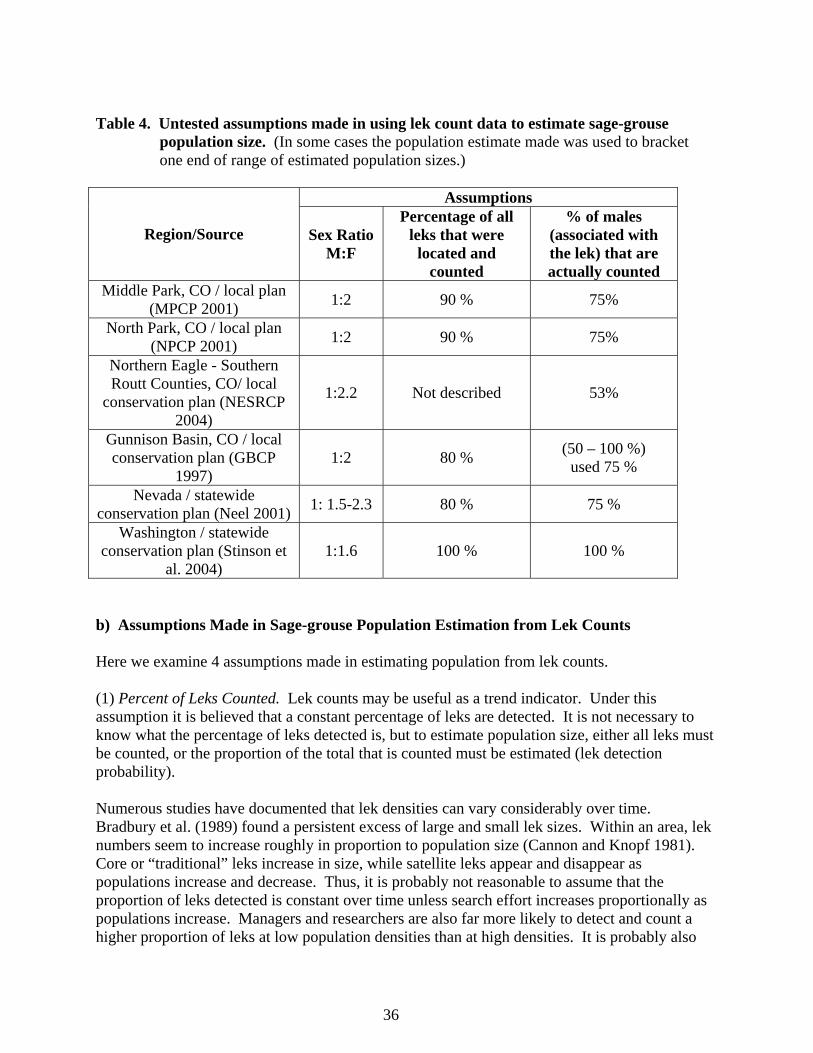
The publication advises caution in the interpretation of counts because of the high level of variance in the data, but no additional aid in interpretation of lek count data is given. The committee’s most recent guidelines (Connelly et al. 2000c) also suggest viewing lek data with caution, but state that lek counts (per Autenreith et al. 1982) provide the best index to breeding population levels. In an extension of that assumption, Connelly et al. (2000c) reaffirm specific statements from Connelly and Braun (1997) that suggest there has been a 17 - 47% decline in breeding populations across their range. Applegate (2000) and Anderson (2001) pointed out that index data cannot be extrapolated to estimates of animal density or abundance unless the proportion of the total population that is counted in the index method is known. For sage-grouse populations, this depends on (1) the proportion of leks that are known and counted; (2) the number and timing of counts conducted; (3) time of day in which counts are conducted; (4) lek attendance rates by yearling and adult males; and (5) the sex ratio of the population. All of these parameters are likely to vary significantly spatially and over time, yet when population estimates are derived from lek count data these parameters are assumed to be fixed constants. Lek count data have been used to make inferences about sage-grouse population trends for at least 50 years, without any credible scientific investigation into the relationship between lek counts and population size. Because of the interest in having population estimates for sage-grouse (and because of the lack of other efficient methods for population estimation of sage-grouse), it is now a common practice to use lek data to estimate the size of various populations of sage-grouse. Multiple untested assumptions are often made in using lek count data to estimate sage-grouse population size (Table 4). These usually include assumptions regarding population sex ratio, an estimate of the percentage of leks that are counted, and the percent of males in the population that are counted at leks. The Washington State Recovery Plan for Greater Sage-grouse (Stinson et al. 2004) also mentions that males could make inter-lek movements, but does not address this in its estimates (Stinson et al. 2004).

36

Table 4. Untested assumptions made in using lek count data to estimate sage-grouse population size. (In some cases the population estimate made was used to bracket one end of range of estimated population sizes.)

Assumptions

Region/Source

Sex Ratio M:F

Percentage of all leks that were

located and counted

% of males (associated with the lek) that are actually counted

Middle Park, CO / local plan (MPCP 2001) 1:2 90 % 75%

North Park, CO / local plan (NPCP 2001) 1:2 90 % 75%

Northern Eagle - Southern Routt Counties, CO/ local

conservation plan (NESRCP 2004)

1:2.2 Not described 53%

Gunnison Basin, CO / local conservation plan (GBCP

1997) 1:2 80 % (50 – 100 %)

used 75 %

Nevada / statewide conservation plan (Neel 2001) 1: 1.5-2.3 80 % 75 %

Washington / statewide conservation plan (Stinson et

al. 2004) 1:1.6 100 % 100 %

b) Assumptions Made in Sage-grouse Population Estimation from Lek Counts Here we examine 4 assumptions made in estimating population from lek counts.

(1) Percent of Leks Counted. Lek counts may be useful as a trend indicator. Under this assumption it is believed that a constant percentage of leks are detected. It is not necessary to know what the percentage of leks detected is, but to estimate population size, either all leks must be counted, or the proportion of the total that is counted must be estimated (lek detection probability). Numerous studies have documented that lek densities can vary considerably over time. Bradbury et al. (1989) found a persistent excess of large and small lek sizes. Within an area, lek numbers seem to increase roughly in proportion to population size (Cannon and Knopf 1981). Core or “traditional” leks increase in size, while satellite leks appear and disappear as populations increase and decrease. Thus, it is probably not reasonable to assume that the proportion of leks detected is constant over time unless search effort increases proportionally as populations increase. Managers and researchers are also far more likely to detect and count a higher proportion of leks at low population densities than at high densities. It is probably also

37

not reasonable to assume potentially active leks are of “average” size, because potentially active leks are more likely to be satellite leks and thus smaller. Lastly, because detectability may be a function of number of males, larger leks may be more noticeable.

(2) Inter-lek Movements. Attendance by males at more than 1 lek is problematic, because birds may be counted multiple times at different leks, thus inflating population estimates, or they may not be counted at all if they are attending a different lek when counts occur. The ability of lek counts to serve as an index to population trends will not be affected by inter-lek movements if the movements are relatively constant from year to year. Unfortunately, inter-lek movements are both significant and variable. Dalke et al. (1963) reported inter-lek movements by individual (banded) adult males varied by year from 22 - 47%. Dunn and Braun (1985) recorded no marked birds moving between leks in 1982, but 14 of 91 (15%) were observed at 2 or more leks in 1983. Emmons and Braun (1984) reported all (11) juvenile males attended from 2-4 leks during the breeding season, while inter-lek movements of adults were infrequent (3 of 11; 27%).

(3) Lek Attendance. Population estimates from lek count data assume that a constant proportion of males, often 75%, are detected by the maximum of 3-4 counts (e.g., Table 4). There is considerable evidence that lek attendance is highly variable due to age, social status, weather, body condition, and parasite load or disease. Patterson (1952:152) suggested that all males regularly attended leks, although the only data he presented to support this assertion was: “All these marked birds were identified morning after morning occupying the same territory on the strutting ground.” He was examining marked birds with respect to territoriality in this reference, and the marking referred to birds he captured on leks and dyed, or birds he identified by tail feather patterns. Dalke et al. (1963:820) didn’t calculate attendance rate for banded birds, but indicated that “…banded males were ordinarily absent from the strutting grounds from 1 to 3 days at a time…”, and “The less dominant males were irregular in their visitations. The dominant males were present almost daily under all conditions.” Dalke et al. (1963:822) also noted, “Banded males were often seen in the sagebrush adjacent to the strutting grounds,” although this was attributed to trapping disturbance. Hartzler (1972) documented males with almost daily lek attendance and others that only sporadically attended leks in Montana. Wiley (1973a) stated that there was an abundance of males that didn’t attend leks, and he further speculated (Wiley 1974) that attendance patterns of males were likely to be a function of density (lek size). Dunn and Braun (1985) reported daily attendance rate of marked adult males was only 43%, ranging from 3-96% for individual males. Daily attendance by yearling males was only 33% (Dunn and Braun 1985). One bias in assessing attendance based on observations of banded birds is that apparent low attendance may be caused by mortality of banded birds. Emmons and Braun (1984:1023) studied male sage-grouse lek attendance with the objective “…to examine the daily attendance patterns on leks of male sage-grouse during the breeding season,” but lumped attendance across 5-day, 15-day, or season-long averages. Although their data indicated significant within-year and across-year variation even when lumped into 5-day intervals, they did not report what fraction of radio-marked males would be detected by normal counting protocols. Since 93% of the birds they based their attendance rates on were trapped while night-roosting on leks, it is probable they (and others) caught highly territorial, dominant males who regularly attend leks, and thus it is likely the estimate of lek attendance may be biased high.

38

The physical condition of sage-grouse can also affect their attendance at leks. Hupp and Braun (1989a) found that sage-grouse had depleted lipid and protein reserves following a severe winter in Colorado. This, and snow cover, caused the birds to largely delay initiating display activities until late April. There was substantial variation in lipid reserves across 3 years, which could impact lek attendance and display rates. The authors noted substantially higher variation in lek counts within a season for GuSG than for GrSG in North Park. Boyce (1990) reported that males with avian malaria were significantly less likely to attend leks than males without malaria, and that malaria varied spatially and temporally across 11 leks in southeast Wyoming. Thus, disease prevalence has the potential to impact attendance rates and lek counts, and variability in disease prevalence may increase variability in attendance rates. Walsh et al. (2004) studied attendance rates of radio-marked and color-banded male and female sage-grouse captured during winter in Middle Park, Colorado during 1 mating season. They found male daily attendance rates were highly variable (7-86% for adults, and 0-42% for yearlings), and influenced by age, date, and time of day. They documented that counts conducted between half an hour after sunrise and 1.5 hours after sunrise (typical when managers count more than 1 lek in a morning) detected only 74% and 44% of the actual high count of adults and yearlings for that day, respectively.

(4) Sex Ratio. Most population estimates derived from lek counts assume 2 females/males in the breeding population (e.g., Table 4). This assumption is based on long-term wing data obtained by determining sex and age of wings obtained at wing barrels or check stations (CDOW, unpublished report). It is apparent both from wing data and from population modeling that sex ratios vary markedly from year to year. This is because males encounter higher mortality rates as they mature and enter the breeding population (Zablan et al. 2003). Therefore the sex ratio will be a function of the age structure of the population; older age-structured populations will have high female-to-male sex ratios because this differential mortality will have had longer to operate. Following years of above average recruitment, populations will have female-to-male sex ratios closer to 1:1, since yearling and first-year adults will dominate the population and will have experienced little differential mortality. Sex ratios for all age classes (immature, yearling, and adult) of GrSG from wing data (CDOW, unpublished report) yielded varying sex ratios. In Middle Park from 1976 – 1993, wing data yielded 1.5 ± 0.5 females/male. In Northwest Colorado wing data yielded 1.6 ± 0.4 females/male from 1976 – 1998. In North Park, from 1974-1998 wing data yielded a sex ratio of 1.7 ± 0.3 females/male. More specifically in Northwest Colorado, Cold Springs, Blue Mountain, and Central Moffat County wing data yielded sex ratios of 1.8 ± 0.5, 1.4 ± 0.4, and 1.6 ± 0.3 females/male, respectively. We assume that a constant sex ratio is not defensible since it masks annual variability in nature. The long-term (1974 – 1998) average sex ratio for all GrSG age classes in Colorado was 1.6 ± 0.4 females/male, which is significantly lower than the 2.0 females/male that is typically used in population estimation equations. c) Alternative Methods of Population Estimation Given the unreliability of the assumptions used, how do estimates derived from them compare to other, more rigorous estimates? Using mark-recapture statistical techniques, Walsh (2002)

39

estimated the size of adult and yearling male and female GrSG populations in Middle Park during 1 breeding season. He compared them to population estimates derived from lek counts using standard assumptions (90% of leks are known and counted, 75% of males are counted, and there are 2 females/male in the population). He found that adjusted lek count estimates underestimated population size from mark-recapture estimates by 28%, because attendance rates were much lower than assumed and there were more females (2.3/male) than assumed. Stiver, using mark-recapture techniques, estimated there were 53 male and 115 female GuSG in San Miguel County in Colorado in the spring of 2003 (J. Stiver, University of Nebraska, personal communication). Extrapolation from the maximum of 4 lek counts using standard assumptions listed above yielded estimates of 41 males and 82 females, underestimating the mark-resight estimates by 23 and 29 %, respectively. The maximum of 4 counts of males represented only 53% of the male population (as estimated by mark-resight), well below the assumed 75%. Thus, estimates of population size extrapolated from lek count data using standard assumptions appear to significantly underestimate population sizes. Mark-recapture methods have shown promise in developing population estimates with confidence intervals, but the difficulty in capturing and marking the proportion of the population necessary (Walsh 2002) suggest it will be practical only for small populations. Recent research (Wilson et al. 2003) has explored using individual DNA as a marker, eliminating the need to handle and mark individual birds. The CDOW is exploring the utility of using DNA assayed from fecal droppings (collected on leks) as a mark-recapture technique. CDOW will also explore the practicality of using other methods to estimate lek and/or population density such as line-transects (Burnham et al. 1980). CDOW will continue to test the assumptions about male attendance and sex ratios implicit in estimating population size from traditional lek counts. d) Conclusions

It is not defensible to generate breeding population estimates for sage-grouse from lek counts by assuming that (1) all (or some fraction of) leks are known; (2) potentially active leks are of average size; (3) the maximum of 3 or 4 counts represents 75% of the males in the population; (4) there are exactly 2 (or any fixed ratio) females per male in the population; and (5) there is no variability in the assumptions across time, space, or population size. Unfortunately, that does not diminish the need for population estimates. It is difficult to evaluate past population trends, or to assess where we are relative to population targets or population viability without estimates of current population size. Either new methods need to be developed, or assumptions used to extrapolate from lek counts need to be evaluated and refined. Estimating population size of GrSG by whatever means will be expensive and potentially disruptive to individual sage-grouse at varying levels. In the long-term, annual estimates of population size are probably unnecessary and may be counter-productive from the standpoint of diverting resources and impacting birds. Currently annual lek counts represent the only method for monitoring trends in GrSG populations, and should be continued until better, more precise estimates can be obtained. Therefore, even though we recognize the lack of statistical reliability, we estimate population sizes from lek counts. They are the only long-term index available to document trends. However, for the purposes of this Plan, to eliminate at least one parameter with

40

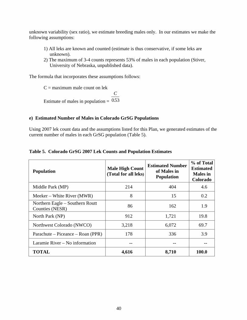
unknown variability (sex ratio), we estimate breeding males only. In our estimates we make the following assumptions: 1) All leks are known and counted (estimate is thus conservative, if some leks are unknown). 2) The maximum of 3-4 counts represents 53% of males in each population (Stiver, University of Nebraska, unpublished data). The formula that incorporates these assumptions follows: C = maximum male count on lek

Estimate of males in population = C

0 53. e) Estimated Number of Males in Colorado GrSG Populations Using 2007 lek count data and the assumptions listed for this Plan, we generated estimates of the current number of males in each GrSG population (Table 5). Table 5. Colorado GrSG 2007 Lek Counts and Population Estimates

Population Male High Count(Total for all leks)

Estimated Number of Males in Population

% of Total Estimated Males in Colorado

Middle Park (MP) 214 404 4.6

Meeker – White River (MWR) 8 15 0.2 Northern Eagle – Southern Routt Counties (NESR) 86 162 1.9

North Park (NP) 912 1,721 19.8

Northwest Colorado (NWCO) 3,218 6,072 69.7

Parachute – Piceance – Roan (PPR) 178 336 3.9

Laramie River – No information -- -- --

TOTAL 4,616 8,710 100.0

41

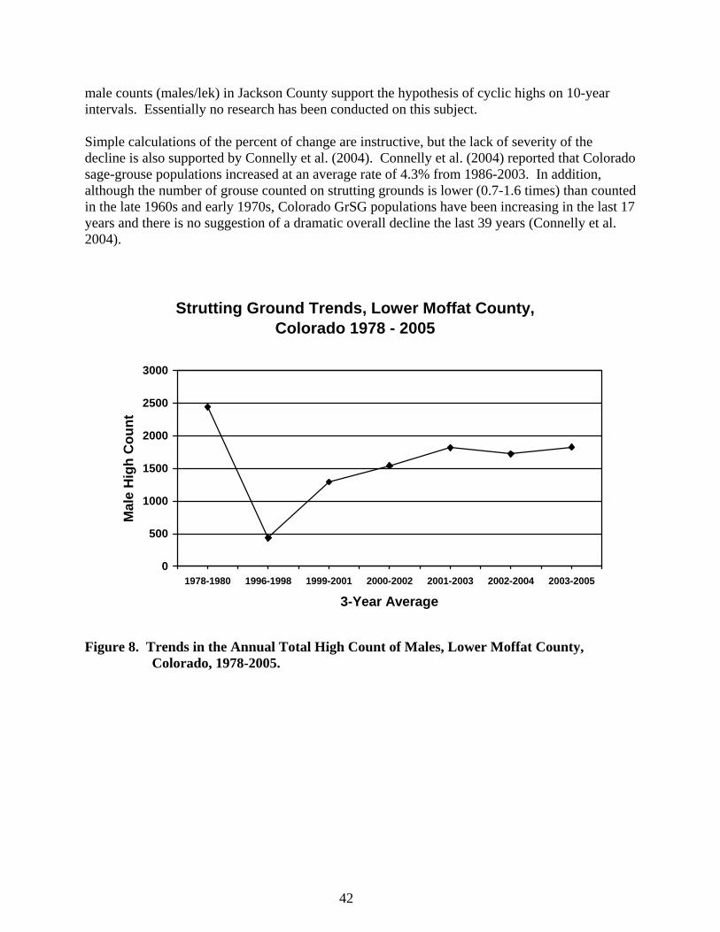
f) Decline of Greater Sage-grouse In Colorado, GrSG historically occurred in at least 13 counties (Braun 1995). GrSG have been extirpated in Lake and Chaffee counties, and for 2 other counties sage-grouse have also been lost, although whether they were GrSG or GuSG is not certain (see Fig. 3). Braun (1995) suggested that Greater Sage-Grouse are currently found in 9 Colorado counties. He considered populations with more than 500 breeding GrSG (totals of males and females in the spring) as persistent, and concluded that persistent populations were found in Jackson, Moffat, Rio Blanco, and Routt counties. Populations Braun (1995:6) considered “at risk” of extirpation include Larimer, Grand, Summit, Eagle, and Garfield counties. Although Braun (1995) considered the populations in 4 counties secure, he did not cite any original reference to clarify or justify the basis for “500 breeding individuals” constituting a secure population. Following further review of the literature (in an attempt to support or refute the validity of the 500 breeding male benchmark) this Plan will assume that the 500 breeding individual estimate was derived from Franklin (1980) and Soulé (1980). Those authors proposed that a population (or “effective” population) of 500 is sufficient for long-term maintenance of genetic variability in a population. Lande (1988) suggests that this number was quickly adopted as the basis of management plans for captive and wild populations. Additionally, Lande (1995a) suggested that in experiments with fruit flies (Drosophila melanogaster), a population size of 5,000 is necessary rather than the Franklin-Soulé number of 500. Lande (1995a) cautioned using the value of 5,000 because of differences among characters and species in genetic mutations and environmental fluctuations. Later, Connelly and Braun (1997:230) suggested that grouse populations in Colorado were “at risk,” although earlier Braun (1995:6) concluded that the major populations in Colorado were “persistent.” Connelly and Braun (1997:230) did not provide any definition of the term “at risk”. Connelly and Braun (1997) also argued that breeding populations (males/lek) of sage-grouse decreased by 33% across GrSG range, and males/lek declined by 31% and chicks/hen declined by 10% in Colorado since 1984. Braun (1998) further emphasized the population decline in Colorado and reported an 82% decline in lower Moffat County (all of Moffat County excluding the Cold Springs and Blue Mountain areas), in the three-year average of the number of strutting males counted on leks between 1978-80 and 1996-98. Braun (1998) concluded that there had been a 57% decrease in the number of active leks during the same time period. More recent and updated calculations (Fig. 8) suggest that the declines are not as severe as suggested by Braun (1998). Counts of strutting have been conducted in the same areas. If the 1978-80 timeframe is used as the “benchmark,” the current lek counts illustrate a 25% decrease in the number of strutting males, a 20% increase in the number of active leks, and a 38% decrease in the number of males/lek in the latest 3-year running average (Figs. 8 and 9). Although there has been a decline in the number of males counted from the 1978-1980 period, the decline in Moffat County has not been as severe as Braun (1998) concluded. These dramatic shifts in numbers of strutting males may be a result of the hypothesized cyclic nature of greater sage-grouse populations (Rich 1985, Braun 1998). Braun (1998) suggested that the strutting

42

Strutting Ground Trends, Lower Moffat County, Colorado 1978 - 2005

0

500

1000

1500

2000

2500

3000

1978-1980 1996-1998 1999-2001 2000-2002 2001-2003 2002-2004 2003-2005

3-Year Average

Mal

e H

igh

Cou

nt

male counts (males/lek) in Jackson County support the hypothesis of cyclic highs on 10-year intervals. Essentially no research has been conducted on this subject. Simple calculations of the percent of change are instructive, but the lack of severity of the decline is also supported by Connelly et al. (2004). Connelly et al. (2004) reported that Colorado sage-grouse populations increased at an average rate of 4.3% from 1986-2003. In addition, although the number of grouse counted on strutting grounds is lower (0.7-1.6 times) than counted in the late 1960s and early 1970s, Colorado GrSG populations have been increasing in the last 17 years and there is no suggestion of a dramatic overall decline the last 39 years (Connelly et al. 2004).

Figure 8. Trends in the Annual Total High Count of Males, Lower Moffat County, Colorado, 1978-2005.

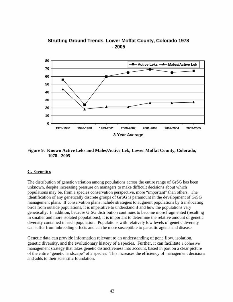
43

Strutting Ground Trends, Lower Moffat County, Colorado 1978 - 2005

0

10

20

30

40

50

60

70

80

1978-1980 1996-1998 1999-2001 2000-2002 2001-2003 2002-2004 2003-2005

3-Year Average

Active Leks Males/Active Lek

Figure 9. Known Active Leks and Males/Active Lek, Lower Moffat County, Colorado, 1978 - 2005 C. Genetics The distribution of genetic variation among populations across the entire range of GrSG has been unknown, despite increasing pressure on managers to make difficult decisions about which populations may be, from a species conservation perspective, more “important” than others. The identification of any genetically discrete groups of GrSG is paramount in the development of GrSG management plans. If conservation plans include strategies to augment populations by translocating birds from outside populations, it is imperative to understand if and how the populations vary genetically. In addition, because GrSG distribution continues to become more fragmented (resulting in smaller and more isolated populations), it is important to determine the relative amount of genetic diversity contained in each population. Populations with relatively low levels of genetic diversity can suffer from inbreeding effects and can be more susceptible to parasitic agents and disease. Genetic data can provide information relevant to an understanding of gene flow, isolation, genetic diversity, and the evolutionary history of a species. Further, it can facilitate a cohesive management strategy that takes genetic distinctiveness into account, based in part on a clear picture of the entire “genetic landscape” of a species. This increases the efficiency of management decisions and adds to their scientific foundation.

44

Previous population genetic studies of sage-grouse have focused on assessing taxonomic status (Kahn et al. 1999, Oyler-McCance et al. 1999, Benedict et al. 2003). These studies provided useful taxonomic information and knowledge of the distribution of genetic variation locally, yet they lacked the range-wide perspective necessary to make management decisions regarding GrSG at the species level. A recently completed analysis of the PPR population compared with 5 other Greater Sage-grouse populations in Colorado (Laramie River not included) revealed that the genetic make-up of PPR is generally consistent with the other 5 populations (Oyler-McCance, 2007). Using mtDNA sequence data, 5 of the 8 haplotypes found in PPR (66% of the PPR birds) were also found in the other populations in Colorado. Of the three PPR haplotypes not found in Colorado, 2 (EU and W) were found in the neighboring states of Utah and Wyoming. One haplotype was unique to PPR (New3) and at relatively high frequency (20%). Two other Colorado populations (Blue Mountain and Cold Springs) each also had a unique haplotype representing 10 and 8% of the populations respectively (Oyler-McCance et al. 2005a). The PPR population had a much higher sample size (65 compared to ~ 20 in the other populations) and the sampling method was different (trapped birds in PPR vs. hunter killed birds in the rest of the Colorado birds), which may influence the potential for relatedness among samples. Additionally, the PPR population did have similar levels of genetic diversity (both in the number of haplotypes and in haplotypes diversity) as the other Colorado populations, and again, a higher sample size likely resulted in more haplotypes being identified. Nonetheless, it appears that the PPR population does not suffer from low diversity and appears to have diversity levels that are comparable to the other Colorado populations. The mtDNA neighbor-joining network, which was constructed using FST genetic distances among populations, suggests that PPR is more closely related to North Park, Cold Springs, and Blue Mountain, than to Middle Park and Eagle. The fact that PPR is not shown to have branch lengths longer than the other Colorado populations suggests that it is not genetically distinct from all other Colorado Greater Sage-grouse populations. The microsatellite data are relatively concordant with that of the mtDNA data. The STRUCTURE analysis found that the most appropriate number of discrete genetic clusters (K) was 1 given the data from these 6 populations, suggesting that there was little genetic structure within the data. Pairwise population RST tests, based on allele frequencies of populations, revealed a few significant differences among populations yet these differences were primarily between Cold Springs and the other populations. This finding is highlighted with the microsatellite neighbor-joining network that shows Cold Springs as the most genetically distinct population. This network suggests that PPR is more closely related to Middle Park and Eagle, contrary to the network built with mtDNA data. This discrepancy is likely due to the different patterns of inheritance of these two types of genetic markers (maternal vs. bi-parental). An additional factor that could lead to minor differences between the two data sets has to do with the number of loci sampled (sampling error). While the mitochondrial genome represents one locus, multiple sites were sampled in the nuclear genome. Levels of genetic diversity in PPR were again similar to what had been previously been reported for populations in Colorado (Oyler-McCance et al. 2005a). The levels of mean observed heterozygosity in PPR were the lowest reported in Colorado yet the values are only slightly lower than those reported elsewhere (0.55 as opposed to 0.61-0.69). This could be due to a number of factors including smaller population sizes, increased fragmentation among sagebrush habitat resulting in sampled birds being more

45

related, or merely due to the different sampling method used in this study (trapped birds vs. hunter killed birds). 1) Summary The study by Oyler-McCance et al. (2005) documented the distribution of genetic variation across the entire range of GrSG. They found that isolation by distance has left an imprint on GrSG gene pools, and that local adaptation is a realistic possibility for the species that should be considered in decisions involving translocations. They argue that this genetic data used in conjunction with large scale demographic and habitat data will provide an integrated approach to conservation efforts for GrSG. For Colorado, there appears to be a genetic line of demarcation (north to south) between Colorado GrSG populations, suggesting that if translocations are undertaken, birds should be moved north – south, and not east – west. In summary, the Greater Sage-Grouse in PPR do not appear to be substantially different from other Greater Sage-grouse sampled in Colorado. There is some level of uniqueness (as represented by the new haplotype found in 20% of the PPR birds) yet this is not unusual as both Cold Springs and Blue Mountain also contained haplotypes that were unique to that particular population. Additionally, the levels of genetic diversity in PPR do appear to be comparable to other populations although they were reported to have the lowest levels of observed heterozygosity levels. D. Greater Sage-grouse Habitat Mapping Efforts 1) Colorado Conservation Plan (CCP) Habitat Mapping CDOW is using the Wildlife Resource Information System (WRIS) and GrSG habitat use data to map GrSG habitat. The following habitat definitions were used during the initial mapping portion of this project, and appear in maps in the PPR Plan. Future mapping should also focus on distinguishing between areas that are “Suitable and Vacant”, vs. those that are “Suitable but Unknown”. In addition, initial mapping of these habitats was done at a fairly coarse level and is not suitable for project-level planning. More detailed mapping will be necessary for specific projects. Occupied Habitat: Areas of suitable habitat known to be used by GrSG within the last 10 years from the date of mapping. Areas of suitable habitat contiguous with areas of known use, which do not have effective barriers to sage-grouse movement from known use areas, are mapped as occupied habitat unless specific information exists that documents the lack of sage-grouse use. This category can be delineated from any combination of telemetry locations, sightings of sage-grouse or sage-grouse sign, local biological expertise, GIS analysis, or other data sources. Vacant or Unknown Habitat: Suitable habitat for sage-grouse that is separated (not contiguous)

from occupied habitats that either (1) has not been adequately inventoried, or (2) has not had documentation of grouse presence in the past 10 years.

46

Potentially Suitable Habitat: Unoccupied habitats that could be suitable for occupation of sage- grouse if practical restoration were applied. Soils or other historic information (photos, maps, reports, etc.) indicate sagebrush communities occupied these areas. As examples, these sites could include areas overtaken by piñon-juniper or converted to rangeland.

2) BLM State Habitat Mapping A mapping effort was also initiated by the Colorado BLM in 2002, through a contract with the Colorado Natural Heritage Program (CNHP), as part of a national agency mapping effort. With the help of other agency biologists, the Colorado BLM completed a statewide habitat risk map. BLM and CDOW biologists (primarily) hand-edited spatial information about sagebrush and sage-grouse habitats on 1:100,000 topographic maps based on Basin-wide vegetation inventory data and local knowledge of the area. They identified existing sage-grouse habitat in Colorado that appears to be in good condition, as well as habitat that is “at risk.” For those habitats considered to be at risk, biologists identified the specific issue(s) potentially affecting the habitat (e.g., weeds, fire, lack of fire), and whether the “risk” threatened habitat quality or might result in habitat loss and/or fragmentation. In identifying habitat quality (“good” or “at risk”), biologists also considered whether the habitat quality in a habitat polygon was likely to significantly degrade within 5 years if no management actions were taken. CNHP organized, compiled, facilitated and produced the results of this mapping effort. These maps were not included in this Plan due to their large size; they are available at local BLM field offices. Four habitat quality risk factors were identified: (1) weed invasion; (2) piñon-juniper encroachment; (3) old and even-aged sagebrush overstory; and (4) poor herbaceous understory condition. Six factors causing habitat loss or fragmentation were noted: (1) weed domination; (2) piñon-juniper replacement; (3) oil and gas development; (4) powerline infrastructure development; (5) subdivisions (human development); and (6) existing or proposed land-uses (ranging from land exchange to agricultural conversion). For each polygon, any occurrence of sage-grouse was noted, and site-specific comments (e.g., wildfire, gravel pit, weed infestation associated with oil field) were recorded. The BLM habitat map will be updated every 5 years to reflect changes in habitat due to management, new information, or a consequence of nature (e.g., drought, fire, disease). These maps are expected to help identify and prioritize BLM budget, conservation actions, and management for sage-grouse on public lands. The maps will also be made available to other agencies and local work groups to use as a tool in sage-grouse management proposals and decisions. In addition, BLM has developed a national sage-grouse mapping effort designed to provide range-wide information about the location, status, and trend of GrSG habitats, and the influence of a variety of land-uses/disturbances on those habitats. This modeling effort is not intended to portray quality of existing habitat, but rather to depict relative connectivity of existing sagebrush ecosystems across the West. Colorado GrSG habitats fall within 2 regions covered by this project, the Wyoming Basins Region in the northwest portion of the state, and the Colorado Plateau Region. This project was spearheaded by the National Science and Technology Center in Denver. BLM, CDOW, and other biologists had an opportunity to review and validate some of the modeling assumptions that were used in this GIS mapping exercise. These maps may be

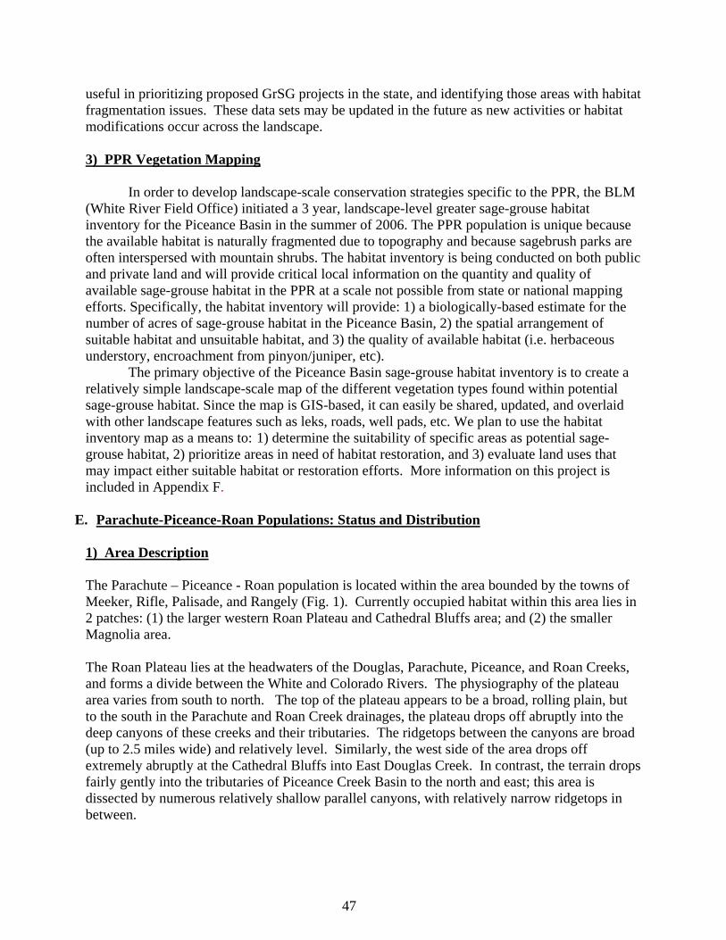
47

useful in prioritizing proposed GrSG projects in the state, and identifying those areas with habitat fragmentation issues. These data sets may be updated in the future as new activities or habitat modifications occur across the landscape. 3) PPR Vegetation Mapping

In order to develop landscape-scale conservation strategies specific to the PPR, the BLM (White River Field Office) initiated a 3 year, landscape-level greater sage-grouse habitat inventory for the Piceance Basin in the summer of 2006. The PPR population is unique because the available habitat is naturally fragmented due to topography and because sagebrush parks are often interspersed with mountain shrubs. The habitat inventory is being conducted on both public and private land and will provide critical local information on the quantity and quality of available sage-grouse habitat in the PPR at a scale not possible from state or national mapping efforts. Specifically, the habitat inventory will provide: 1) a biologically-based estimate for the number of acres of sage-grouse habitat in the Piceance Basin, 2) the spatial arrangement of suitable habitat and unsuitable habitat, and 3) the quality of available habitat (i.e. herbaceous understory, encroachment from pinyon/juniper, etc). The primary objective of the Piceance Basin sage-grouse habitat inventory is to create a relatively simple landscape-scale map of the different vegetation types found within potential sage-grouse habitat. Since the map is GIS-based, it can easily be shared, updated, and overlaid with other landscape features such as leks, roads, well pads, etc. We plan to use the habitat inventory map as a means to: 1) determine the suitability of specific areas as potential sage-grouse habitat, 2) prioritize areas in need of habitat restoration, and 3) evaluate land uses that may impact either suitable habitat or restoration efforts. More information on this project is included in Appendix F.

E. Parachute-Piceance-Roan Populations: Status and Distribution 1) Area Description The Parachute – Piceance - Roan population is located within the area bounded by the towns of Meeker, Rifle, Palisade, and Rangely (Fig. 1). Currently occupied habitat within this area lies in 2 patches: (1) the larger western Roan Plateau and Cathedral Bluffs area; and (2) the smaller Magnolia area. The Roan Plateau lies at the headwaters of the Douglas, Parachute, Piceance, and Roan Creeks, and forms a divide between the White and Colorado Rivers. The physiography of the plateau area varies from south to north. The top of the plateau appears to be a broad, rolling plain, but to the south in the Parachute and Roan Creek drainages, the plateau drops off abruptly into the deep canyons of these creeks and their tributaries. The ridgetops between the canyons are broad (up to 2.5 miles wide) and relatively level. Similarly, the west side of the area drops off extremely abruptly at the Cathedral Bluffs into East Douglas Creek. In contrast, the terrain drops fairly gently into the tributaries of Piceance Creek Basin to the north and east; this area is dissected by numerous relatively shallow parallel canyons, with relatively narrow ridgetops in between.

48

The majority of the birds in the PPR population inhabit the higher elevations (7000-8900 ft.) of the Parachute, Piceance, and Roan Creek drainages. Some of the headwater areas of East Douglas Creek (Cathedral, Lake and Soldier Creeks) are within this area as well. A small group of birds inhabit the Magnolia area, in the higher elevations (approximately 6500-7500 feet) of Greasewood and Collins gulches, north of Piceance Creek. The maximum elevation of approximately 8950 feet occurs on the west side of the Square S Summer Range (CDOW property) at the headwaters of Brush Creek and Soldier creeks. Precipitation within occupied habitat in the PPR ranges from 16-25 inches per year, varying primarily with elevation (Fig. 11). Vegetation cover also varies from south to north. On the southern, lower ends of the ridges between Parachute and Roan Creeks and their tributaries, mountain shrub communities (a mix of serviceberry, Gambel's oak, bitterbrush, and big sagebrush) dominate, interspersed with patches of big sagebrush and aspen, depending on topography. Aspen pockets are found on north to northeast facing slopes, and sagebrush appears along gentle slopes in the bottoms of washes. Ridgetops to the north are dominated by big sagebrush, and aspen pockets are found on the northern slopes, occasionally on the ridges. This situation holds along the highest ridges forming the White River - Colorado River divide, as well as along the Cathedral Bluffs to the north. In the Piceance Creek drainage, mountain shrub is a lesser component, found on north-facing slopes only, with big sagebrush on ridgetops, and as one travels north or northeast downs these ridgetops, piñon and juniper woodlands are more prevalent, and appear to be encroaching into the sagebrush as time has passed over the years. The Magnolia area is similar in this regard. In the PPR population area, sage-grouse are largely restricted to sagebrush-covered ridges and plateaus at higher elevations, whereas slopes with mountain shrubs and narrow valley bottoms (even those with some sagebrush) are not used (Fig. 12). Mountain shrub communities, particularly serviceberry, are more common and extensive in PPR than elsewhere in GrSG range. Serviceberry is well-established in the PPR, with dense areas of serviceberry occupying the lower and drier ridges within occupied habitat. Big sagebrush is the dominant shrub species in the highest elevations of occupied GrSG habitat, but is interspersed with serviceberry in many locations. While PPR sage-grouse have been demonstrated to use the margins of serviceberry stands for nesting and brood-rearing habitat, higher lek counts occur where sagebrush is the dominant shrub. Landownership within Occupied Habitat is approximately 65% private and 35% public (see Table 6 and Fig. 10) and overall 46% and 54% respectively. On the south side, in the Parachute and Roan drainages, approximately 90% is private, and a large portion of that is owned by large energy corporations. To the north in the Piceance Basin, a majority is in public ownership, particularly at the lower elevations, with the exception of canyon bottoms along streams, which tend to be privately held. The traditional land-use in the area has been domestic livestock grazing. However, the potential for large-scale energy resource development has been recognized since the discovery and patenting of oil shale claims in the 1920s. The presence of oil shale and natural gas in the area accounts for the large proportion of ownership by energy companies. Currently, natural gas development is rapidly expanding in the area as pipelines tied into national supply networks have been constructed and prices have risen. Residential development is not a factor in the area at this time, although there is the possibility that worker camps will be constructed within sage-grouse habitat as gas development increases, due to the

49

remote locations of this activity from towns and the difficult nature of travel in this rugged country.

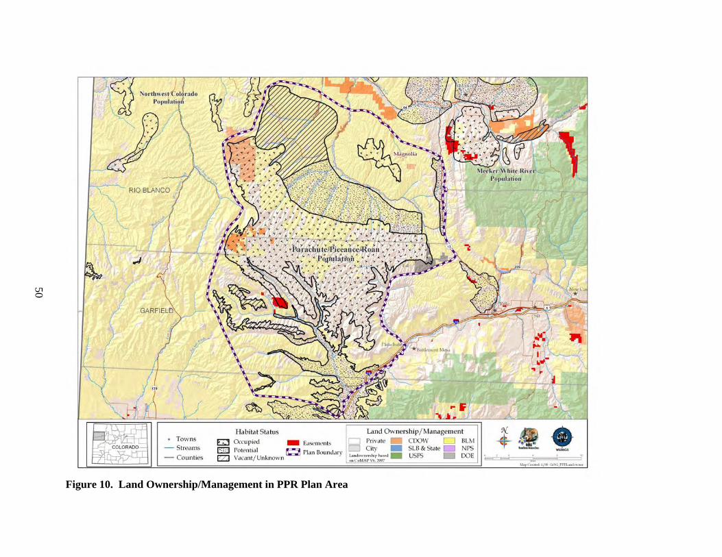
50

Figure 10. Land Ownership/Management in PPR Plan Area

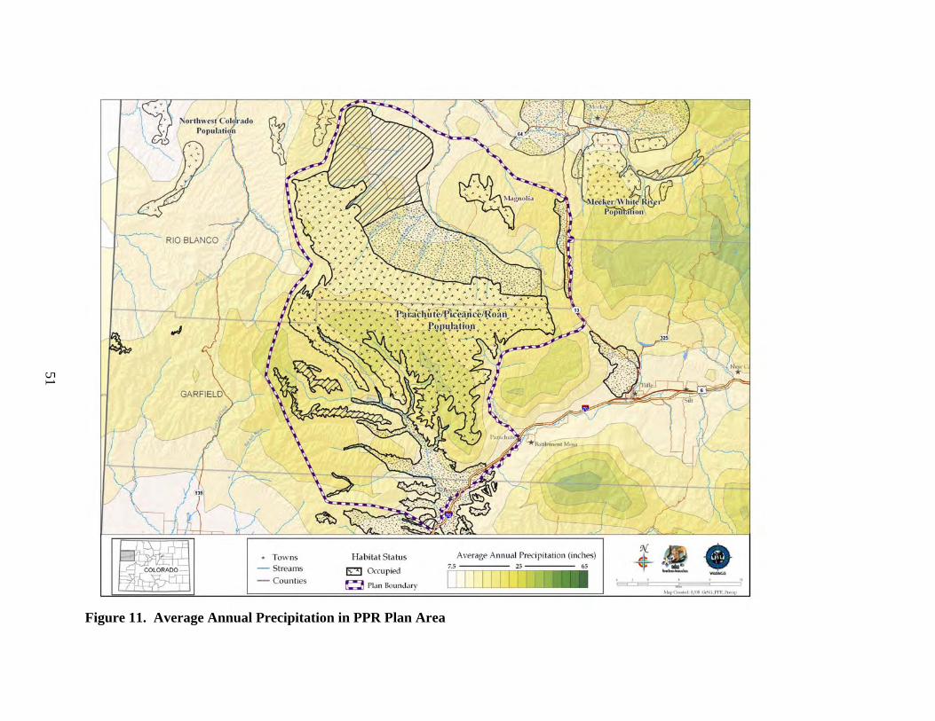
51

Figure 11. Average Annual Precipitation in PPR Plan Area

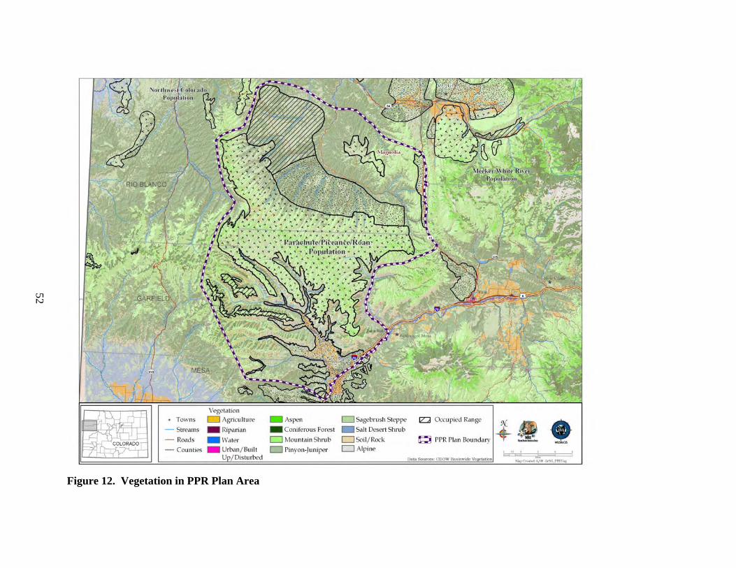
52

Figure 12. Vegetation in PPR Plan Area

53

The Parachute/Piceance/Roan population of GrSG is found in Rio Blanco and Garfield counties in northwest Colorado. The majority of the population is found south of Piceance Creek, but a small group of birds remain near the Magnolia Energy Camp at the head of Greasewood Gulch in T2S R96W. Piceance Creek has numerous tributaries separated by long narrow ridges that generally run south to north and southwest to northeast. Valleys between the ridges are rarely greater than 500 feet deep. The ridge tops vary in width from 500 yards to 2 miles and from ¾ mile to over 20 miles in length. The Roan Creek and Parachute Creek drainages are characterized by deep canyons often exceeding 1000 feet with nearly vertical walls and several spectacular waterfalls. The current Wildlife Resource Information System (WRIS) map on the CDOW website (Natural Diversity Information Source [NDIS] 2007. http://ndis.nrel.colostate.edu/wildlifespx.asp?SpCode=041201) for the PPR population includes 304,588 acres of Occupied Habitat, 99,683 acres of Vacant/Unknown Habitat, and 221,788 acres of Potentially Suitable Habitat (Table 6). Habitat for the PPR population is naturally fragmented because the birds live in sagebrush communities on ridgetops that are separated by deep drainages. In addition, the elevation on precipitation and temperature and soils interact to produce an extremely diverse vegetative mosaic. Many areas on the ridges and surrounding slopes are hard to classify in terms of vegetative composition – standing in one spot, one could literally reach out and touch the major components of three or even four major vegetation communities – sagebrush, serviceberry, Gambel’s oak, pinyon pine, juniper, and aspen. This terrain and vegetation mosaic makes the PPR habitats distinct from the habitats of other GrSG populations in Colorado. Classic GrSG habitat provides large expanses of sagebrush on gently rolling terrain. The area is considered semi-arid with a wide range of temperatures and weather conditions. Climatalogical data were taken from the NOAA website (http://www.wrcc.dri.edu/summary/Climsmco.html) for two sites closest to the range occupied by the population of birds: one at the Altenbern Ranch in Roan Creek (58 years of data) and the other at the Little Hills facility owned by the Colorado Division of Wildlife (CDOW) on the Dry Fork of Piceance Creek (43 years of data). The data for both sites was averaged with mean annual precipitation at 15.14 inches, average annual snowfall at 59.4 inches, mean maximum temperature 61.9 degrees F and mean minimum temperature 27.3 degrees F. In the general area, snowfall accounts for about 50% of the total precipitation. The lowest temperature recorded was -48 degrees F and the highest was 104 degrees F. The average annual precipitation at the upper elevation where the majority of the birds live should equal or slightly exceed that observed at the two weather reporting stations which are at lower elevations. Soil type, elevation, slope and aspect determine the vegetation at any given site. Three subspecies of big sagebrush (Artemesia tridentata) can be found in the area, with basin big sagebrush (A. t. tridentata) most common in the drainage bottoms below 6500 feet in elevation. Wyoming big sagebrush (A.t. wyomingensis) is found on ridges between 6200 and 6600 feet in elevation, and mountain big sagebrush (A. t. vaseyana) is prevalent at elevations above 6800 feet (Cottrell and Bonham 1992).

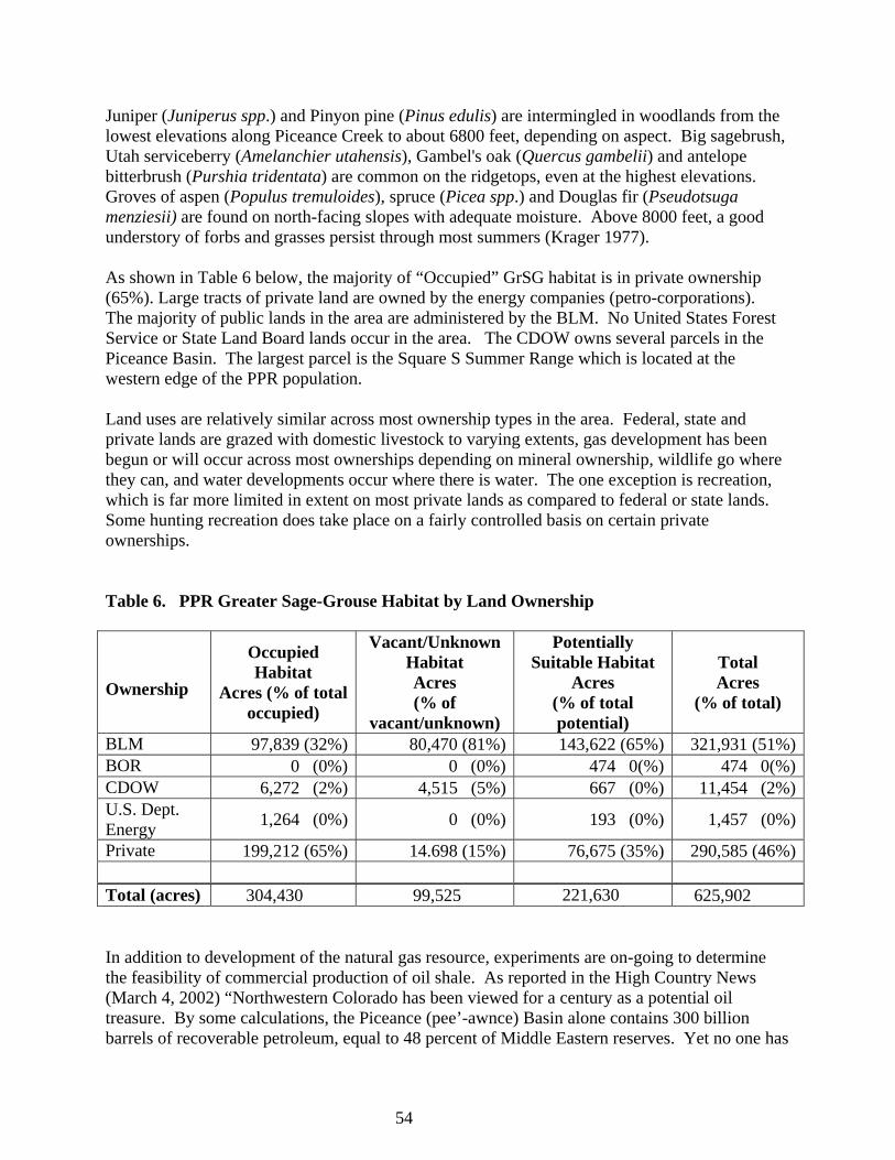
54

Juniper (Juniperus spp.) and Pinyon pine (Pinus edulis) are intermingled in woodlands from the lowest elevations along Piceance Creek to about 6800 feet, depending on aspect. Big sagebrush, Utah serviceberry (Amelanchier utahensis), Gambel's oak (Quercus gambelii) and antelope bitterbrush (Purshia tridentata) are common on the ridgetops, even at the highest elevations. Groves of aspen (Populus tremuloides), spruce (Picea spp.) and Douglas fir (Pseudotsuga menziesii) are found on north-facing slopes with adequate moisture. Above 8000 feet, a good understory of forbs and grasses persist through most summers (Krager 1977). As shown in Table 6 below, the majority of “Occupied” GrSG habitat is in private ownership (65%). Large tracts of private land are owned by the energy companies (petro-corporations). The majority of public lands in the area are administered by the BLM. No United States Forest Service or State Land Board lands occur in the area. The CDOW owns several parcels in the Piceance Basin. The largest parcel is the Square S Summer Range which is located at the western edge of the PPR population. Land uses are relatively similar across most ownership types in the area. Federal, state and private lands are grazed with domestic livestock to varying extents, gas development has been begun or will occur across most ownerships depending on mineral ownership, wildlife go where they can, and water developments occur where there is water. The one exception is recreation, which is far more limited in extent on most private lands as compared to federal or state lands. Some hunting recreation does take place on a fairly controlled basis on certain private ownerships. Table 6. PPR Greater Sage-Grouse Habitat by Land Ownership

Ownership

Occupied Habitat

Acres (% of total occupied)

Vacant/Unknown Habitat Acres (% of

vacant/unknown)

Potentially Suitable Habitat

Acres (% of total potential)

Total Acres

(% of total)

BLM 97,839 (32%) 80,470 (81%) 143,622 (65%) 321,931 (51%)BOR 0 (0%) 0 (0%) 474 0(%) 474 0(%)CDOW 6,272 (2%) 4,515 (5%) 667 (0%) 11,454 (2%)U.S. Dept. Energy 1,264 (0%) 0 (0%) 193 (0%) 1,457 (0%)

Private 199,212 (65%) 14.698 (15%) 76,675 (35%) 290,585 (46%) Total (acres) 304,430 99,525 221,630 625,902 In addition to development of the natural gas resource, experiments are on-going to determine the feasibility of commercial production of oil shale. As reported in the High Country News (March 4, 2002) “Northwestern Colorado has been viewed for a century as a potential oil treasure. By some calculations, the Piceance (pee’-awnce) Basin alone contains 300 billion barrels of recoverable petroleum, equal to 48 percent of Middle Eastern reserves. Yet no one has

55

been able to extract profitably the keragen, a waxy petroleum, from the shale.” More than 70% of the total oil shale acreage in the Green River Formation, including the richest and thickest oil shale deposits, is under federally owned and managed lands (Oil Shale & Tar Sands Programmatic EIS Information Center. http://ostseis.anl.gov/guide/oilshale/index.cfm). Currently, the BLM has issued leases for 5 experimental operations in Colorado’s Piceance Basin to test different technologies to extract oil from the shale deposits. Facilities to extract sodium bicarbonate have been built in the Piceance Basin (hydrologic) from underground nacolite deposits; only one of the facilities is still in operation. Grazing by domestic sheep and cattle started in the area in the 1870’s. Currently, there are few sheep and a fraction of the cattle numbers that were historically driven to the summer range at higher elevations and then wintered along the bottoms in the three major drainages. 2) Population Information Leks in the PPR are concentrated at high elevations and remote locations, particularly in the Parachute - Roan portion of this population. Many of these leks are inaccessible from the ground during optimal periods for lek counts due to snow and mud conditions. This makes consistent lek counts difficult to accomplish, complicating comparison of data among years. Aerial lek counts have been the only possible method for counting sage-grouse on leks for some of the PPR. These aerial counts have historically been conducted by fixed-wing aircraft, which results in reduced sightability of birds and less consistent counts from year to year. CDOW has used helicopter surveys in 2005, 2006, and 2007 to count leks in this population. These counts have resulted in substantially higher counts that so far appear more consistent among years. Extensive field work in 1975-77 provided the first complete look at sage-grouse distribution and numbers in the PPR (high male count = 234 in 1976; Krager 1977). Lek counts conducted by CDOW in the spring 2005, (the most exhaustive count completed since 1976), yielded a high male count of 180 birds, followed by high counts of 226 and 178 in 2006 and 2007, respectively (Fig. 13). Because of the limited amount of consistent data available, it is too soon to describe any trend in this population. Note that, for the purposes of documenting trends, we report only the number of GrSG males counted, not the total population size (see Fig. 13). Going forward from 2007, the primary trend indicator will be the 3-year running average of high male lek counts. A three-year running average dampens annual fluctuations in annual counts that may be caused by variables such as weather conditions affecting the birds or the conduct of count flights, variations in observer expertise, and lek accessibility. The triangle on the graph on the next page represents the first data point of the three-year running average (195 males)

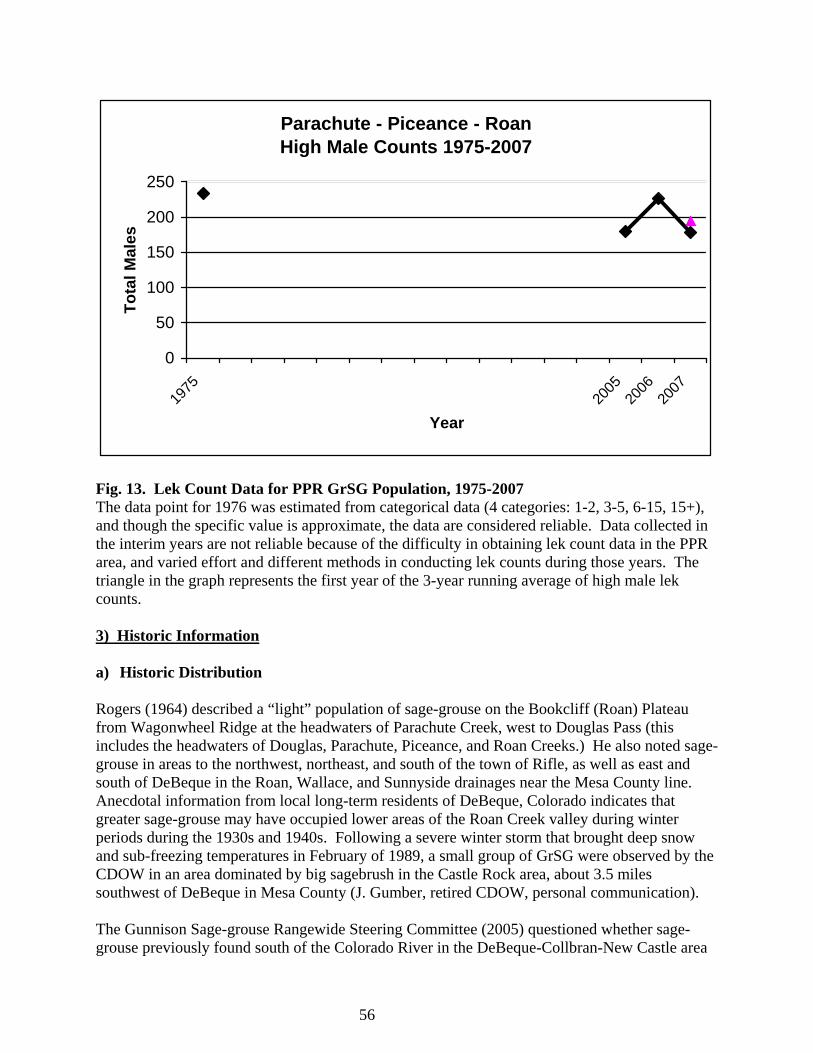
56

Parachute - Piceance - Roan High Male Counts 1975-2007

0

50

100

150

200

250

1975

2005

2006

2007

Year

Tota

l Mal

es

Fig. 13. Lek Count Data for PPR GrSG Population, 1975-2007 The data point for 1976 was estimated from categorical data (4 categories: 1-2, 3-5, 6-15, 15+), and though the specific value is approximate, the data are considered reliable. Data collected in the interim years are not reliable because of the difficulty in obtaining lek count data in the PPR area, and varied effort and different methods in conducting lek counts during those years. The triangle in the graph represents the first year of the 3-year running average of high male lek counts. 3) Historic Information a) Historic Distribution

Rogers (1964) described a “light” population of sage-grouse on the Bookcliff (Roan) Plateau from Wagonwheel Ridge at the headwaters of Parachute Creek, west to Douglas Pass (this includes the headwaters of Douglas, Parachute, Piceance, and Roan Creeks.) He also noted sage-grouse in areas to the northwest, northeast, and south of the town of Rifle, as well as east and south of DeBeque in the Roan, Wallace, and Sunnyside drainages near the Mesa County line. Anecdotal information from local long-term residents of DeBeque, Colorado indicates that greater sage-grouse may have occupied lower areas of the Roan Creek valley during winter periods during the 1930s and 1940s. Following a severe winter storm that brought deep snow and sub-freezing temperatures in February of 1989, a small group of GrSG were observed by the CDOW in an area dominated by big sagebrush in the Castle Rock area, about 3.5 miles southwest of DeBeque in Mesa County (J. Gumber, retired CDOW, personal communication). The Gunnison Sage-grouse Rangewide Steering Committee (2005) questioned whether sage-grouse previously found south of the Colorado River in the DeBeque-Collbran-New Castle area

57

are GrSG or GuSG. No published evidence exists to prove this one way or another, but a river as small as the Colorado would not present a barrier to travel by sage-grouse. Sage-grouse are strong fliers and have the ability to cross a river the size of the Mississippi. Regardless, sage-grouse have been extirpated south of the Colorado River in Garfield and northeastern Mesa counties, as well as north of the Colorado River and east of Parachute Creek in Eastern Garfield County. b) Population Monitoring Rogers (1964) reported only three strutting grounds (leks) in Garfield County and two in Rio Blanco County. In Garfield County, one lek was near Harvey Gap Reservoir, one on West Coulter Creek and one on Hunter Mesa south of Rifle. There have been no birds in those areas for decades. In Rio Blanco County, the known leks were 84 Mesa, south of Duck Creek, and Oil Wells, Little Hills near the present-day Magnolia Energy Camp. Birds are present in only one of those five areas today, but the total number of known leks is now over 80. Much of the difficulty in obtaining counts in the mid-1900’s was a shortage of field personnel to search for and inventory leks and the difficulty in reaching much of the area occupied by the birds during the breeding season. The old adage, “You can’t get there from here” applies to much of the PPR in the late winter/early spring. Many of the leks were “discovered” by searches in fixed-wing aircraft in the 1970’s. Ron Krager (1977) found 28 “new” (previously unreported) leks flying systematic searches along ridges during the breeding seasons of 1975-77. Appendix E includes a map of currently known leks and lek status definitions. Many of the lek locations were plotted on USGS topographic maps from the front seat of a fixed-wing aircraft flying at 100 mph, so lek locations may not be exact. Some work remains to ground-truth lek locations, eliminate duplication and determine current status. This appendix also contains CDOW definitions of lek status: active, inactive, historic and potentially active. After Krager’s work in the 1970’s, lek inventories were conducted each spring, some by ground counts but most by fixed-wing aircraft. In some years, scheduling and weather problems precluded the flights, so the data set is lacking, especially when you consider that CDOW guidelines for lek counts call for a minimum of 3 counts of each lek between March 15 and May 15. In some years, only lek “activity” checks were conducted to determine if the lek site had been visited by GrSG that spring; numbers of birds on leks was not determined. More than anything else, the data set reflects the difficulty in reaching the lek sites for accurate counts. To inventory the leks of the PPR population requires a greater effort than anywhere else in Colorado. In most areas of the state, CDOW field personnel can access leks by vehicle and complete multiple counts of each lek each spring, while the PPR leks require aerial surveys which are more difficult, weather-dependent, and less accurate. During the winter 2005-06, the ad hoc committee that preceded formation of the working group determined that a more aggressive inventory effort should be conducted. Because of the access issues described above, it was decided that multiple helicopter flights would provide the best data. Over $21,000 was donated to the CDOW by energy-related companies. Six helicopter flights were conducted, three on each side of the drainage divide, plus three fixed-wing flights

58

were conducted for the southern portion of the population. Flying both fixed-wing and helicopter counts allowed for comparison of the efficacy of each method. The increased effort and the use of the helicopter resulted in the observation of many more birds on the lek, and discovery of several new lek locations. The same inventory effort, with the helicopter flights paid for largely by industry, was conducted in 2006. The donations collected in early 2005 paid for the 2005 and the majority of the 2006 helicopter flights.

The following list provides a comparison of the advantages of each aircraft:

• Helicopters are more maneuverable. The approach to the lek can easily be made from varying directions, which provides the observer numerous angles of light/view to detect the grouse, without flushing the birds from repeated flyovers.

• Helicopters can approach the lek more slowly and allow the observer(s) more time to view the birds.

• Helicopters can fly lower and closer to the lek providing a better view of the grouse– the fixed wing aircraft stays 500-700 feet off the surface while the helicopter can hover if necessary below 300 feet.

• Fixed wing aircraft generally tend to flush birds even at higher aircraft altitudes, probably due to the raptor-like shape of the fixed-wing aircraft.

• Fixed wing counts provide more consistency of data. Only two years of data from helicopter counts are available, but the data set from fixed wing counts covers many years.

• Distances between the leks can be covered more quickly with the fixed wing. • Fixed wing flights are much less expensive. In 2005, DBS Helicopters from Rifle

provided the aircraft at a cost of $875 per flight hour; in 2006, Heliquest Helicopters from Grand Junction flew the counts at a cost of $750 per hour. The 2007 flights were done with Olathe Spray Service at $644.00/hr. The DOW regional fixed wing aircraft (Cessna 185) can be operated at a cost of $150 per flight hour (2005 estimates).

• More accurate lek locations (UTM coordinates) can be determined with a helicopter. It’s difficult to obtain the exact coordinates from a fixed wing aircraft that is moving 80-100 mph.

Data from lek counts on the south side allow comparison of fixed-wing and helicopter counts. In 2006 as well as in 2005, the counts on the south side of the Piceance-Roan/Parachute Divide were flown with both the fixed-wing aircraft and helicopter. In 2005, the high count with the helicopter was 84 birds while 45 birds were observed from the fixed-wing; this computes to 87% more birds being seen from the helicopter. In 2006, the high count was 154 birds observed from the helicopter and 83 from the fixed-wing; thus 86% more birds were seen from the helicopter. It seems clear that use of the helicopter results in many more birds observed. The downside is the expense; at current prices it costs approximately $12,000 to fly the six counts each spring with the helicopter while the CDOW fixed-wing aircraft requires no additional expenditure. 4) Local Conservation Plan Efforts to develop a local conservation Plan began in the summer of 2005. Informational meetings were held in Roan Creek, Piceance Creek, and Parachute in June 2005, and a Work Group was formed in July, 2005. Work Group meetings have been held monthly since then, and

59

work on the Plan is progressing steadily, with expected Plan completion in early 2008 (PPRCP 2008). The most complex issue the Work Group has addressed is energy and mineral development (and associated infrastructure). Other issues include grazing, predation, habitat quality, recreation, piñon-juniper encroachment, and water development. Strategies have been developed for all issues and final preparation of the Plan is in progress. The Work Group has decided that it will not set a specific population goal or target because of the lack of a consistent, long-term data set, a lack of perspective as to how current data fits into a long-term trend, and a general sense of uncertainty both about the past population numbers and projected natural gas development in the area. The data problems are discussed below. The lack of perspective comes from looking at the graph of counts from 2005-2007 (Fig. 13). Three data points on a graph cannot provide a realistic, defensible indication of where we’ve been, upward or downward trend, or even where this population is in relation to other populations in Colorado. This general uncertainty comes from concerns revolving around potential federal listing of the bird, the Population Viability Analysis in the Statewide Conservation Plan and the potentially gloomy potential forecasts put forth therein. The Work Group is acutely aware of the potential problems facing sage-grouse in the area and is dedicated to addressing these problems. At this time, the Work Group will not establish population objectives until sufficient data is collected. Instead, the group intends to conduct a detailed annual analysis of what has gone on during the previous year followed by recommendations on addressing issues that appear to be negatively influencing grouse and/or their habitat. More details on this process later in this narrative. Determination of a population objective for the Parachute-Piceance-Roan population of Greater Sage-Grouse is a difficult issue compared to some other Colorado populations. Lek count data, the flawed but primary method of estimating a population, are far more intermittent and variable for this population than for others in NW Colorado. North Park has thirty+ years of consistent data; NW Colorado has nine years, etc. Essentially, there are very few years of quality lek count data for this population: 1976 (flawed as well, but more complete than anything prior to 2005), and 2005 to the present. This Plan contains strategies to improve data collection (see “Data Collection and Management” section). The lack of a long-term quality data set presents difficulties in attempting to determine a population objective. One reason for setting a population objective is to have some kind of objective or goal to maintain or strive for. It’s also inherently interesting to know how things are going from one year to the next with a wildlife population that is of interest. When looking at these types of numbers, it’s natural to wonder what is “normal.” When there is concern for a species’ long term survival, and petitions to list a species as “Threatened” or “Endangered,” questions of past and present population levels become more urgent. This is the situation as this Plan is being written in no small part to address concerns for this sage-grouse population. What we know about the PPR population is that in 1976, a minimum of 204 males were counted; in 2005, 184 males were counted, 226 in 2006, and 178 in 2007. These are really the only years that something remotely approximating an “apples to apples” comparison can be made (though even this is a stretch, since the 1976 counts were with fixed wing aircraft only, and not all known leks were counted). In all of the other years beginning with the first counts in 1962, there

60

isvariation in the amount of effort, the type of count (ground, fixed wing aircraft or helicopter), the number of leks visited, the number of times leks were visited, whether any effort was made at all, etc. All of those years are “oranges” to the “apples” of 1976 and 2005 onward. A graph representing the numbers of males counted over the years from 1962 to the present is totally misleading and ultimately meaningless and is not presented here. So what can we say about males lek counts over the years? We can say there were probably around 234 males in 1976 (as estimated from categorical data); we don’t know if that represents a high or low number compared to the years around it, or before that or after that until 2005. We can say that there were more males on leks in 1976 than in 2005-2007. We can speculate that since the some of the leks that had birds in 1976 on the northwestern end of the population no longer have birds, and most of the other general areas of leks continue to have birds, that it stands to reason that if the total area of occupied habitat has decreased, there would be fewer birds now than in 1976. But we still don’t know whether 1976’s 234 males represent a high, medium, or low number for years prior to 2005. As if there isn’t enough variability, the comparison between numbers in 1976 and recent (2005 on) is confounded by different count methods (fixed wing aircraft in 1976, helicopters recently). Comparisons between fixed wing counts and helicopter counts in the years 2005-2007 suggest that a fixed wing flight counts roughly 60% of the birds seen on helicopter flights, which could mean the 1976 number could have been substantially higher if helicopters had been used on the count. For a detailed explanation of how the 1976 number was determined, see Appendix D. The Work Group decided during its deliberations over the draft Plan that Conservation Action 4d. (p. 92) should apply not only to energy-related activities, but to any disturbance activity that may appear to be leading to a downward trend in lek counts. Where a 3 year consecutive downward trend in lek counts (as measured by the 3-year running average) is seen in the area as a whole and/or portions of the area, consider aggressively pursuing additional strategies to address population sustainability including:

• options for increasing GrSG female survival; • shorter duration of disturbances and expedition of reclamation:

See “Population Augmentation” strategy section of Statewide Plan for GrSG.

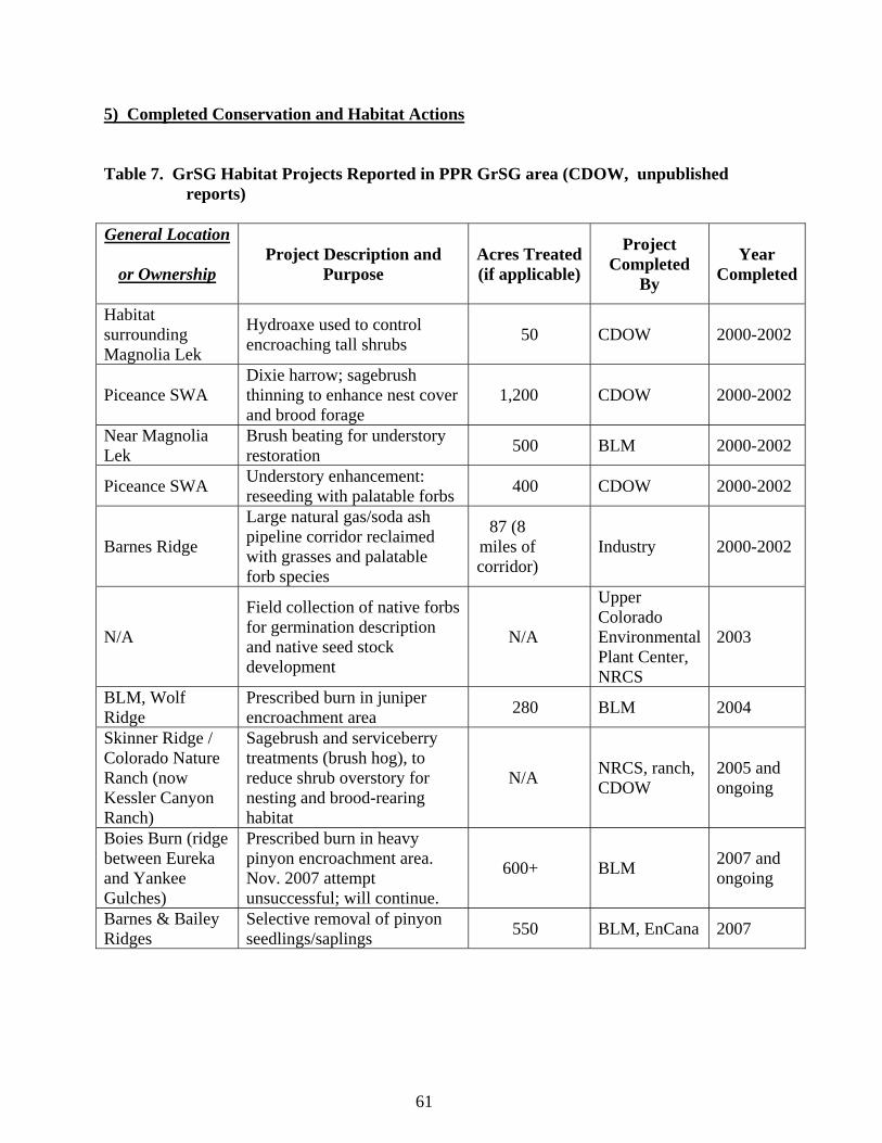
61

5) Completed Conservation and Habitat Actions Table 7. GrSG Habitat Projects Reported in PPR GrSG area (CDOW, unpublished reports) General Location

or Ownership Project Description and

Purpose Acres Treated(if applicable)

Project Completed

By

Year Completed

Habitat surrounding Magnolia Lek

Hydroaxe used to control encroaching tall shrubs 50 CDOW 2000-2002

Piceance SWA Dixie harrow; sagebrush thinning to enhance nest cover and brood forage

1,200 CDOW 2000-2002

Near Magnolia Lek

Brush beating for understory restoration 500 BLM 2000-2002

Piceance SWA Understory enhancement: reseeding with palatable forbs 400 CDOW 2000-2002

Barnes Ridge

Large natural gas/soda ash pipeline corridor reclaimed with grasses and palatable forb species

87 (8 miles of corridor)

Industry 2000-2002

N/A

Field collection of native forbs for germination description and native seed stock development

N/A

Upper Colorado Environmental Plant Center, NRCS

2003

BLM, Wolf Ridge

Prescribed burn in juniper encroachment area 280 BLM 2004

Skinner Ridge / Colorado Nature Ranch (now Kessler Canyon Ranch)

Sagebrush and serviceberry treatments (brush hog), to reduce shrub overstory for nesting and brood-rearing habitat

N/A NRCS, ranch, CDOW

2005 and ongoing

Boies Burn (ridge between Eureka and Yankee Gulches)

Prescribed burn in heavy pinyon encroachment area. Nov. 2007 attempt unsuccessful; will continue.

600+ BLM 2007 and ongoing

Barnes & Bailey Ridges

Selective removal of pinyon seedlings/saplings 550 BLM, EnCana 2007

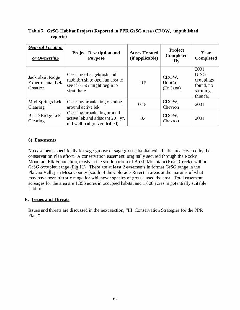
62

Table 7. GrSG Habitat Projects Reported in PPR GrSG area (CDOW, unpublished reports) General Location

or Ownership Project Description and

Purpose Acres Treated(if applicable)

Project Completed

By

Year Completed

Jackrabbit Ridge Experimental Lek Creation

Clearing of sagebrush and rabbitbrush to open an area to see if GrSG might begin to strut there.

0.5 CDOW, UnoCal (EnCana)

2001; GrSG droppings found, no strutting thus far.

Mud Springs Lek Clearing

Clearing/broadening opening around active lek 0.15 CDOW,

Chevron 2001

Bar D Ridge Lek Clearing

Clearing/broadening around active lek and adjacent 20+ yr. old well pad (never drilled)

0.4 CDOW, Chevron 2001

6) Easements No easements specifically for sage-grouse or sage-grouse habitat exist in the area covered by the conservation Plan effort. A conservation easement, originally secured through the Rocky Mountain Elk Foundation, exists in the south portion of Brush Mountain (Roan Creek), within GrSG occupied range (Fig.11). There are at least 2 easements in former GrSG range in the Plateau Valley in Mesa County (south of the Colorado River) in areas at the margins of what may have been historic range for whichever species of grouse used the area. Total easement acreages for the area are 1,355 acres in occupied habitat and 1,808 acres in potentially suitable habitat.

F. Issues and Threats Issues and threats are discussed in the next section, “III. Conservation Strategies for the PPR Plan.”